Author response:
The following is the authors’ response to the original reviews.
eLife Assessment
This valuable study investigates how the neural representation of individual finger movements changes during the early period of sequence learning. By combining a new method for extracting features from human magnetoencephalography data and decoding analyses, the authors provide incomplete evidence of an early, swift change in the brain regions correlated with sequence learning, including a set of previously unreported frontal cortical regions. The addition of more control analyses to rule out that head movement artefacts influence the findings, and to further explain the proposal of offline contextualization during short rest periods as the basis for improvement performance would strengthen the manuscript.
We appreciate the Editorial assessment on our paper’s strengths and novelty. We have implemented additional control analyses to show that neither task-related eye movements nor increasing overlap of finger movements during learning account for our findings, which are that contextualized neural representations in a network of bilateral frontoparietal brain regions actively contribute to skill learning. Importantly, we carried out additional analyses showing that contextualization develops predominantly during rest intervals.
Public Reviews:
Reviewer #1 (Public review):
Summary:
This study addresses the issue of rapid skill learning and whether individual sequence elements (here: finger presses) are differentially represented in human MEG data. The authors use a decoding approach to classify individual finger elements and accomplish an accuracy of around 94%. A relevant finding is that the neural representations of individual finger elements dynamically change over the course of learning. This would be highly relevant for any attempts to develop better brain machine interfaces - one now can decode individual elements within a sequence with high precision, but these representations are not static but develop over the course of learning.
Strengths:
The work follows a large body of work from the same group on the behavioural and neural foundations of sequence learning. The behavioural task is well established and neatly designed to allow for tracking learning and how individual sequence elements contribute. The inclusion of short offline rest periods between learning epochs has been influential because it has revealed that a lot, if not most of the gains in behaviour (ie speed of finger movements) occur in these socalled micro-offline rest periods. The authors use a range of new decoding techniques, and exhaustively interrogate their data in different ways, using different decoding approaches. Regardless of the approach, impressively high decoding accuracies are observed, but when using a hybrid approach that combines the MEG data in different ways, the authors observe decoding accuracies of individual sequence elements from the MEG data of up to 94%.
We have previously showed that neural replay of MEG activity representing the practiced skill was prominent during rest intervals of early learning, and that the replay density correlated with micro-offline gains (Buch et al., 2021). These findings are consistent with recent reports (from two different research groups) that hippocampal ripple density increases during these inter-practice rest periods, and predict offline learning gains (Chen et al., 2024; Sjøgård et al., 2024). However, decoder performance in our earlier work (Buch et al., 2021) left room for improvement. Here, we reported a strategy to improve decoding accuracy that could benefit future studies of neural replay or BCI using MEG.
Weaknesses:
There are a few concerns which the authors may well be able to resolve. These are not weaknesses as such, but factors that would be helpful to address as these concern potential contributions to the results that one would like to rule out. Regarding the decoding results shown in Figure 2 etc, a concern is that within individual frequency bands, the highest accuracy seems to be within frequencies that match the rate of keypresses. This is a general concern when relating movement to brain activity, so is not specific to decoding as done here. As far as reported, there was no specific restraint to the arm or shoulder, and even then it is conceivable that small head movements would correlate highly with the vigor of individual finger movements. This concern is supported by the highest contribution in decoding accuracy being in middle frontal regions - midline structures that would be specifically sensitive to movement artefacts and don't seem to come to mind as key structures for very simple sequential keypress tasks such as this - and the overall pattern is remarkably symmetrical (despite being a unimanual finger task) and spatially broad. This issue may well be matching the time course of learning, as the vigor and speed of finger presses will also influence the degree to which the arm/shoulder and head move. This is not to say that useful information is contained within either of the frequencies or broadband data. But it raises the question of whether a lot is dominated by movement "artefacts" and one may get a more specific answer if removing any such contributions.
Reviewer #1 expresses concern that the combination of the low-frequency narrow-band decoder results, and the bilateral middle frontal regions displaying the highest average intra-parcel decoding performance across subjects is suggestive that the decoding results could be driven by head movement or other artefacts.
Head movement artefacts are highly unlikely to contribute meaningfully to our results for the following reasons. First, in addition to ICA denoising, all “recordings were visually inspected and marked to denoise segments containing other large amplitude artifacts due to movements” (see Methods). Second, the response pad was positioned in a manner that minimized wrist, arm or more proximal body movements during the task. Third, while online monitoring of head position was not performed for this study, it was assessed at the beginning and at the end of each recording. The head was restrained with an inflatable air bladder, and head movement between the beginning and end of each scan did not exceed 5mm for all participants included in the study.
The Reviewer states a concern that “it is conceivable that small head movements would correlate highly with the vigor of individual finger movements”. We agree that despite the steps taken above, it is possible that minor head movements could still contribute to some remaining variance in the MEG data in our study. However, such correlations between small head movements and finger movements could only meaningfully contribute to decoding performance if: (A) they were consistent and pervasive throughout the recording (which might not be the case if the head movements were related to movement vigor and vigor changed over time); and (B) they systematically varied between different finger movements, and also between the same finger movement performed at different sequence locations (see 5-class decoding performance in Figure 4B). The possibility of any head movement artefacts meeting all these conditions is unlikely. Alternatively, for this task design a much more likely confound could be the contribution of eye movement artefacts to the decoder performance (an issue raised by Reviewer #3 in the comments below).
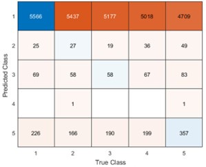
Remember from Figure 1A in the manuscript that an asterisk marks the current position in the sequence and is updated at each keypress. Since participants make very few performance errors, the position of the asterisk on the display is highly correlated with the keypress being made in the sequence. Thus, it is possible that if participants are attending to the visual feedback provided on the display, they may generate eye movements that are systematically related to the task. Since we did record eye movements simultaneously with the MEG recordings (EyeLink 1000 Plus; Fs = 600 Hz), we were able to perform a control analysis to address this question. For each keypress event during trials in which no errors occurred (which is the same time-point that the asterisk position is updated), we extracted three features related to eye movements: 1) the gaze position at the time of asterisk position update (triggered by a KeyDown event), 2) the gaze position 150ms later, and 3) the peak velocity of the eye movement between the two positions. We then constructed a classifier from these features with the aim of predicting the location of the asterisk (ordinal positions 1-5) on the display. As shown in the confusion matrix below (Author response image 1), the classifier failed to perform above chance levels (overall cross-validated accuracy = 0.21817):
Author response image 1.
Confusion matrix showing that three eye movement features fail to predict asterisk position on the task display above chance levels (Fold 1 test accuracy = 0.21718; Fold 2 test accuracy = 0.22023; Fold 3 test accuracy = 0.21859; Fold 4 test accuracy = 0.22113; Fold 5 test accuracy = 0.21373; Overall cross-validated accuracy = 0.2181). Since the ordinal position of the asterisk on the display is highly correlated with the ordinal position of individual keypresses in the sequence, this analysis provides strong evidence that keypress decoding performance from MEG features is not explained by systematic relationships between finger movement behavior and eye movements (i.e. – behavioral artefacts) (end of figure legend).
Remember that the task display does not provide explicit feedback related to performance, only information about the present position in the sequence. Thus, it is possible that participants did not actively attend to the feedback. In fact, inspection of the eye position data revealed that on majority of trials, participants displayed random-walk-like gaze patterns around a central fixation point located near the center of the screen. Thus, participants did not attend to the asterisk position on the display, but instead intrinsically generated the action sequence. A similar realworld example would be manually inputting a long password into a secure online application. In this case, one intrinsically generates the sequence from memory and receives similar feedback about the password sequence position (also provided as asterisks) as provided in the study task – feedback which is typically ignored by the user.
The minimal participant engagement with the visual task display observed in this study highlights another important point – that the behavior in explicit sequence learning motor tasks is highly generative in nature rather than reactive to stimulus cues as in the serial reaction time task (SRTT). This is a crucial difference that must be carefully considered when designing investigations and comparing findings across studies.
We observed that initial keypress decoding accuracy was predominantly driven by contralateral primary sensorimotor cortex in the initial practice trials before transitioning to bilateral frontoparietal regions by trials 11 or 12 as performance gains plateaued. The contribution of contralateral primary sensorimotor areas to early skill learning has been extensively reported in humans and non-human animals.(Buch et al., 2021; Classen et al., 1998; Karni et al., 1995; Kleim et al., 1998) Similarly, the increased involvement of bilateral frontal and parietal regions to decoding during early skill learning in the non-dominant hand is well known. Enhanced bilateral activation in both frontal and parietal cortex during skill learning has been extensively reported (Doyon et al., 2002; Grafton et al., 1992; Hardwick et al., 2013; Kennerley et al., 2004; Shadmehr & Holcomb, 1997; Toni, Ramnani, et al., 2001), and appears to be even more prominent during early fine motor skill learning in the non-dominant hand (Lee et al., 2019; Sawamura et al., 2019). The frontal regions identified in these studies are known to play crucial roles in executive control (Battaglia-Mayer & Caminiti, 2019), motor planning (Toni, Thoenissen, et al., 2001), and working memory (Andersen & Buneo, 2002; Buneo & Andersen, 2006; Shadmehr & Holcomb, 1997; Toni, Ramnani, et al., 2001; Wolpert et al., 1998) processes, while the same parietal regions are known to integrate multimodal sensory feedback and support visuomotor transformations (Andersen & Buneo, 2002; Buneo & Andersen, 2006; Shadmehr & Holcomb, 1997; Toni, Ramnani, et al., 2001; Wolpert et al., 1998), in addition to working memory (Grover et al., 2022). Thus, it is not surprising that these regions increasingly contribute to decoding as subjects internalize the sequential task. We now include a statement reflecting these considerations in the revised Discussion.
A somewhat related point is this: when combining voxel and parcel space, a concern is whether a degree of circularity may have contributed to the improved accuracy of the combined data, because it seems to use the same MEG signals twice - the voxels most contributing are also those contributing most to a parcel being identified as relevant, as parcels reflect the average of voxels within a boundary. In this context, I struggled to understand the explanation given, ie that the improved accuracy of the hybrid model may be due to "lower spatially resolved whole-brain and higher spatially resolved regional activity patterns".
We disagree with the Reviewer’s assertion that the construction of the hybrid-space decoder is circular for the following reasons. First, the base feature set for the hybrid-space decoder constructed for all participants includes whole-brain spatial patterns of MEG source activity averaged within parcels. As stated in the manuscript, these 148 inter-parcel features reflect “lower spatially resolved whole-brain activity patterns” or global brain dynamics. We then independently test how well spatial patterns of MEG source activity for all voxels distributed within individual parcels can decode keypress actions. Again, the testing of these intra-parcel spatial patterns, intended to capture “higher spatially resolved regional brain activity patterns”, is completely independent from one another and independent from the weighting of individual inter-parcel features. These intra-parcel features could, for example, provide additional information about muscle activation patterns or the task environment. These approximately 1150 intra-parcel voxels (on average, within the total number varying between subjects) are then combined with the 148 inter-parcel features to construct the final hybrid-space decoder. In fact, this varied spatial filter approach shares some similarities to the construction of convolutional neural networks (CNNs) used to perform object recognition in image classification applications (Srinivas et al., 2016). One could also view this hybrid-space decoding approach as a spatial analogue to common timefrequency based analyses such as theta-gamma phase amplitude coupling (θ/γ PAC), which assess interactions between two or more narrow-band spectral features derived from the same time-series data (Lisman & Jensen, 2013).
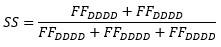
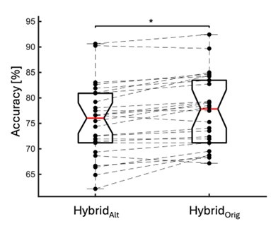
We directly tested this hypothesis – that spatially overlapping intra- and inter-parcel features portray different information – by constructing an alternative hybrid-space decoder (Hybrid<sub>Alt</sub>) that excluded average inter-parcel features which spatially overlapped with intra-parcel voxel features, and comparing the performance to the decoder used in the manuscript (Hybrid<sub>Orig</sub>). The prediction was that if the overlapping parcel contained similar information to the more spatially resolved voxel patterns, then removing the parcel features (n=8) from the decoding analysis should not impact performance. In fact, despite making up less than 1% of the overall input feature space, removing those parcels resulted in a significant drop in overall performance greater than 2% (78.15% ± 7.03% SD for Hybrid<sub>Orig</sub> vs. 75.49% ± 7.17% for Hybrid<sub>Alt</sub>; Wilcoxon signed rank test, z = 3.7410, p = 1.8326e-04; Author response image 2).
Author response image 2.
Comparison of decoding performances with two different hybrid approaches. Hybrid<sub>Alt</sub>: Intra-parcel voxel-space features of top ranked parcels and inter-parcel features of remaining parcels. Hybrid<sub>Orig</sub>: Voxel-space features of top ranked parcels and whole-brain parcel-space features (i.e. – the version used in the manuscript). Dots represent decoding accuracy for individual subjects. Dashed lines indicate the trend in performance change across participants. Note, that Hybrid<sub>Orig</sub> (the approach used in our manuscript) significantly outperforms the Hybrid<sub>Alt</sub> approach, indicating that the excluded parcel features provide unique information compared to the spatially overlapping intra-parcel voxel patterns (end of figure legend).
Firstly, there will be a relatively high degree of spatial contiguity among voxels because of the nature of the signal measured, i.e. nearby individual voxels are unlikely to be independent. Secondly, the voxel data gives a somewhat misleading sense of precision; the inversion can be set up to give an estimate for each voxel, but there will not just be dependence among adjacent voxels, but also substantial variation in the sensitivity and confidence with which activity can be projected to different parts of the brain. Midline and deeper structures come to mind, where the inversion will be more problematic than for regions along the dorsal convexity of the brain, and a concern is that in those midline structures, the highest decoding accuracy is seen.
We agree with the Reviewer that some inter-parcel features representing neighboring (or spatially contiguous) voxels are likely to be correlated, an important confound in connectivity analyses (Colclough et al., 2015; Colclough et al., 2016), not performed in our investigation.
In our study, correlations between adjacent voxels effectively reduce the dimensionality of the input feature space. However, as long as there are multiple groups of correlated voxels within each parcel (i.e. – the rank is greater than 1), the intra-parcel spatial patterns could meaningfully contribute to the decoder performance, as shown by the following results:
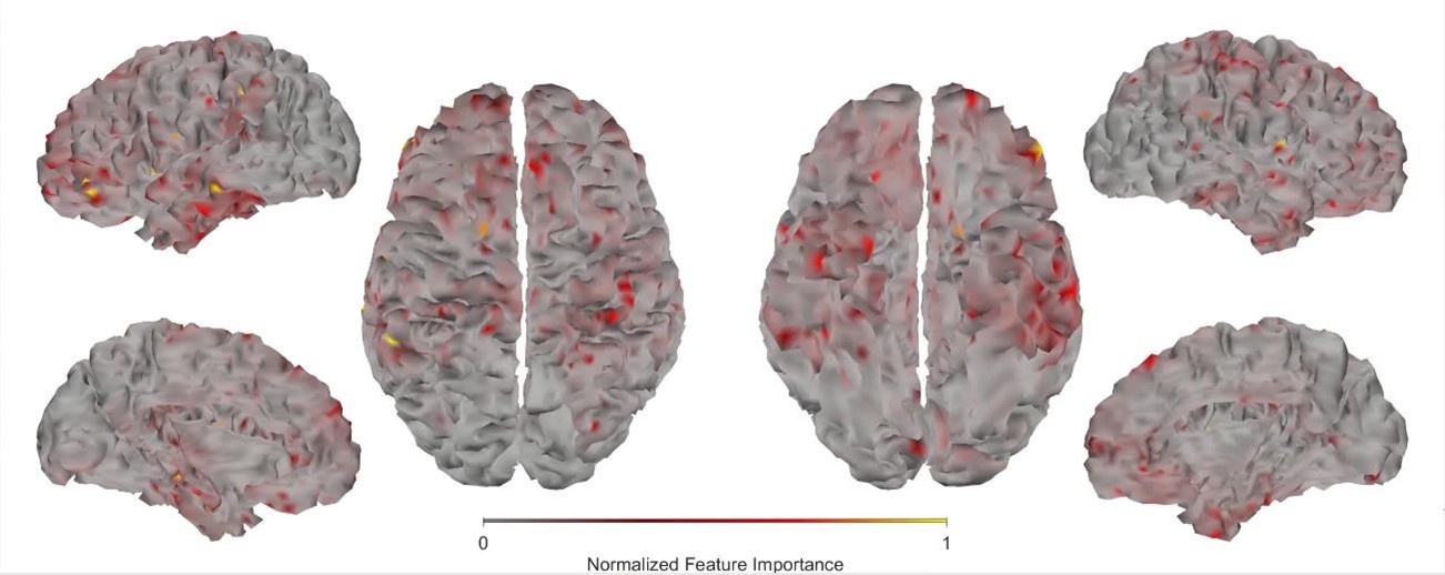
First, we obtained higher decoding accuracy with voxel-space features (74.51% ± 7.34% SD) compared to parcel space features (68.77% ± 7.6%; Figure 3B), indicating individual voxels carry more information in decoding the keypresses than the averaged voxel-space features or parcel space features. Second, individual voxels within a parcel showed varying feature importance scores in decoding keypresses (Author response image 3). This finding shows that correlated voxels form mini subclusters that are much smaller spatially than the parcel they reside within.
Author response image 3.:
Feature importance score of individual voxels in decoding keypresses: MRMR was used to rank the individual voxel space features in decoding keypresses and the min-max normalized MRMR score was mapped to a structural brain surface. Note that individual voxels within a parcel showed different contribution to decoding (end of figure legend).
Some of these concerns could be addressed by recording head movement (with enough precision) to regress out these contributions. The authors state that head movement was monitored with 3 fiducials, and their time courses ought to provide a way to deal with this issue. The ICA procedure may not have sufficiently dealt with removing movement-related problems, but one could eg relate individual components that were identified to the keypresses as another means for checking. An alternative could be to focus on frequency ranges above the movement frequencies. The accuracy for those still seems impressive and may provide a slightly more biologically plausible assessment.
We have already addressed the issue of movement related artefacts in the first response above. With respect to a focus on frequency ranges above movement frequencies, the Reviewer states the “accuracy for those still seems impressive and may provide a slightly more biologically plausible assessment”. First, it is important to note that cortical delta-band oscillations measured with local field potentials (LFPs) in macaques is known to contain important information related to end-effector kinematics (Bansal et al., 2011; Mollazadeh et al., 2011) muscle activation patterns (Flint et al., 2012) and temporal sequencing (Churchland et al., 2012) during skilled reaching and grasping actions. Thus, there is a substantial body of evidence that low-frequency neural oscillatory activity in this range contains important information about the skill learning behavior investigated in the present study. Second, our own data shows (which the Reviewer also points out) that significant information related to the skill learning behavior is also present in higher frequency bands (see Figure 2A and Figure 3—figure supplement 1). As we pointed out in our earlier response to questions about the hybrid space decoder architecture (see above), it is likely that different, yet complimentary, information is encoded across different temporal frequencies (just as it is encoded across different spatial frequencies) (Heusser et al., 2016). Again, this interpretation is supported by our data as the highest performing classifiers in all cases (when holding all parameters constant) were always constructed from broadband input MEG data (Figure 2A and Figure 3—figure supplement 1).
One question concerns the interpretation of the results shown in Figure 4. They imply that during the course of learning, entirely different brain networks underpin the behaviour. Not only that, but they also include regions that would seem rather unexpected to be key nodes for learning and expressing relatively simple finger sequences, such as here. What then is the biological plausibility of these results? The authors seem to circumnavigate this issue by moving into a distance metric that captures the (neural network) changes over the course of learning, but the discussion seems detached from which regions are actually involved; or they offer a rather broad discussion of the anatomical regions identified here, eg in the context of LFOs, where they merely refer to "frontoparietal regions".
The Reviewer notes the shift in brain networks driving keypress decoding performance between trials 1, 11 and 36 as shown in Figure 4A. The Reviewer questions whether these shifts in brain network states underpinning the skill are biologically plausible, as well as the likelihood that bilateral superior and middle frontal and parietal cortex are important nodes within these networks.
First, previous fMRI work in humans assessed changes in functional connectivity patterns while participants performed a similar sequence learning task to our present study (Bassett et al., 2011). Using a dynamic network analysis approach, Bassett et al. showed that flexibility in the composition of individual network modules (i.e. – changes in functional brain region membership of orthogonal brain networks) is up-regulated in novel learning environments and explains differences in learning rates across individuals. Thus, consistent with our findings, it is likely that functional brain networks rapidly reconfigure during early learning of novel sequential motor skills.
Second, frontoparietal network activity is known to support motor memory encoding during early learning (Albouy et al., 2013; Albouy et al., 2012). For example, reactivation events in the posterior parietal (Qin et al., 1997) and medial prefrontal (Euston et al., 2007; Molle & Born, 2009) cortex (MPFC) have been temporally linked to hippocampal replay, and are posited to support memory consolidation across several memory domains (Frankland & Bontempi, 2005), including motor sequence learning (Albouy et al., 2015; Buch et al., 2021; F. Jacobacci et al., 2020). Further, synchronized interactions between MPFC and hippocampus are more prominent during early as opposed to later learning stages (Albouy et al., 2013; Gais et al., 2007; Sterpenich et al., 2009), perhaps reflecting “redistribution of hippocampal memories to MPFC” (Albouy et al., 2013). MPFC contributes to very early memory formation by learning association between contexts, locations, events and adaptive responses during rapid learning (Euston et al., 2012). Consistently, coupling between hippocampus and MPFC has been shown during initial memory encoding and during subsequent rest (van Kesteren et al., 2010; van Kesteren et al., 2012). Importantly, MPFC activity during initial memory encoding predicts subsequent recall (Wagner et al., 1998). Thus, the spatial map required to encode a motor sequence memory may be “built under the supervision of the prefrontal cortex” (Albouy et al., 2012), also engaged in the development of an abstract representation of the sequence (Ashe et al., 2006). In more abstract terms, the prefrontal, premotor and parietal cortices support novice performance “by deploying attentional and control processes” (Doyon et al., 2009; Hikosaka et al., 2002; Penhune & Steele, 2012) required during early learning (Doyon et al., 2009; Hikosaka et al., 2002; Penhune & Steele, 2012). The dorsolateral prefrontal cortex DLPFC specifically is thought to engage in goal selection and sequence monitoring during early skill practice (Schendan et al., 2003), all consistent with the schema model of declarative memory in which prefrontal cortices play an important role in encoding (Morris, 2006; Tse et al., 2007). Thus, several prefrontal and frontoparietal regions contributing to long term learning (Berlot et al., 2020) are also engaged in early stages of encoding. Altogether, there is strong biological support for the involvement of bilateral prefrontal and frontoparietal regions to decoding during early skill learning. We now address this issue in the revised manuscript.
If I understand correctly, the offline neural representation analysis is in essence the comparison of the last keypress vs the first keypress of the next sequence. In that sense, the activity during offline rest periods is actually not considered. This makes the nomenclature somewhat confusing. While it matches the behavioural analysis, having only key presses one can't do it in any other way, but here the authors actually do have recordings of brain activity during offline rest. So at the very least calling it offline neural representation is misleading to this reviewer because what is compared is activity during the last and during the next keypress, not activity during offline periods. But it also seems a missed opportunity - the authors argue that most of the relevant learning occurs during offline rest periods, yet there is no attempt to actually test whether activity during this period can be useful for the questions at hand here.
We agree with the Reviewer that our previous “offline neural representation” nomenclature could be misinterpreted. In the revised manuscript we refer to this difference as the “offline neural representational change”. Please, note that our previous work did link offline neural activity (i.e. – 16-22 Hz beta power (Bonstrup et al., 2019) and neural replay density (Buch et al., 2021) during inter-practice rest periods) to observed micro-offline gains.
Reviewer #2 (Public review):
Summary
Dash et al. asked whether and how the neural representation of individual finger movements is "contextualized" within a trained sequence during the very early period of sequential skill learning by using decoding of MEG signal. Specifically, they assessed whether/how the same finger presses (pressing index finger) embedded in the different ordinal positions of a practiced sequence (4-1-3-2-4; here, the numbers 1 through 4 correspond to the little through the index fingers of the non-dominant left hand) change their representation (MEG feature). They did this by computing either the decoding accuracy of the index finger at the ordinal positions 1 vs. 5 (index_OP1 vs index_OP5) or pattern distance between index_OP1 vs. index_OP5 at each training trial and found that both the decoding accuracy and the pattern distance progressively increase over the course of learning trials. More interestingly, they also computed the pattern distance for index_OP5 for the last execution of a practice trial vs. index_OP1 for the first execution in the next practice trial (i.e., across the rest period). This "off-line" distance was significantly larger than the "on-line" distance, which was computed within practice trials and predicted micro-offline skill gain. Based on these results, the authors conclude that the differentiation of representation for the identical movement embedded in different positions of a sequential skill ("contextualization") primarily occurs during early skill learning, especially during rest, consistent with the recent theory of the "micro-offline learning" proposed by the authors' group. I think this is an important and timely topic for the field of motor learning and beyond.
Strengths
The specific strengths of the current work are as follows. First, the use of temporally rich neural information (MEG signal) has a large advantage over previous studies testing sequential representations using fMRI. This allowed the authors to examine the earliest period (= the first few minutes of training) of skill learning with finer temporal resolution. Second, through the optimization of MEG feature extraction, the current study achieved extremely high decoding accuracy (approx. 94%) compared to previous works. As claimed by the authors, this is one of the strengths of the paper (but see my comments). Third, although some potential refinement might be needed, comparing "online" and "offline" pattern distance is a neat idea.
Weaknesses
Along with the strengths I raised above, the paper has some weaknesses. First, the pursuit of high decoding accuracy, especially the choice of time points and window length (i.e., 200 msec window starting from 0 msec from key press onset), casts a shadow on the interpretation of the main result. Currently, it is unclear whether the decoding results simply reflect behavioral change or true underlying neural change. As shown in the behavioral data, the key press speed reached 3~4 presses per second already at around the end of the early learning period (11th trial), which means inter-press intervals become as short as 250-330 msec. Thus, in almost more than 60% of training period data, the time window for MEG feature extraction (200 msec) spans around 60% of the inter-press intervals. Considering that the preparation/cueing of subsequent presses starts ahead of the actual press (e.g., Kornysheva et al., 2019) and/or potential online planning (e.g., Ariani and Diedrichsen, 2019), the decoder likely has captured these future press information as well as the signal related to the current key press, independent of the formation of genuine sequential representation (e.g., "contextualization" of individual press). This may also explain the gradual increase in decoding accuracy or pattern distance between index_OP1 vs. index_OP5 (Figure 4C and 5A), which co-occurred with performance improvement, as shorter inter-press intervals are more favorable for the dissociating the two index finger presses followed by different finger presses. The compromised decoding accuracies for the control sequences can be explained in similar logic. Therefore, more careful consideration and elaborated discussion seem necessary when trying to both achieve high-performance decoding and assess early skill learning, as it can impact all the subsequent analyses.
The Reviewer raises the possibility that (given the windowing parameters used in the present study) an increase in “contextualization” with learning could simply reflect faster typing speeds as opposed to an actual change in the underlying neural representation.
We now include a new control analysis that addresses this issue as well as additional re-examination of previously reported results with respect to this issue – all of which are inconsistent with this alternative explanation that “contextualization” reflects a change in mixing of keypress related MEG features as opposed to a change in the underlying representations themselves. As correct sequences are generated at higher and higher speeds over training, MEG activity patterns related to the planning, execution, evaluation and memory of individual keypresses overlap more in time. Thus, increased overlap between the “4” and “1” keypresses (at the start of the sequence) and “2” and “4” keypresses (at the end of the sequence) could artefactually increase contextualization distances even if the underlying neural representations for the individual keypresses remain unchanged. One must also keep in mind that since participants repeat the sequence multiple times within the same trial, a majority of the index finger keypresses are performed adjacent to one another (i.e. - the “4-4” transition marking the end of one sequence and the beginning of the next). Thus, increased overlap between consecutive index finger keypresses as typing speed increased should increase their similarity and mask contextualization related changes to the underlying neural representations.
We addressed this question by conducting a new multivariate regression analysis to directly assess whether the neural representation distance score could be predicted by the 4-1, 2-4 and 4-4 keypress transition times observed for each complete correct sequence (both predictor and response variables were z-score normalized within-subject). The results of this analysis also affirmed that the possible alternative explanation that contextualization effects are simple reflections of increased mixing is not supported by the data (Adjusted R<sup>2</sup> = 0.00431; F = 5.62). We now include this new negative control analysis in the revised manuscript.
We also re-examined our previously reported classification results with respect to this issue. We reasoned that if mixing effects reflecting the ordinal sequence structure is an important driver of the contextualization finding, these effects should be observable in the distribution of decoder misclassifications. For example, “4” keypresses would be more likely to be misclassified as “1” or “2” keypresses (or vice versa) than as “3” keypresses. The confusion matrices presented in Figures 3C and 4B and Figure 3—figure supplement 3A display a distribution of misclassifications that is inconsistent with an alternative mixing effect explanation of contextualization.
Based upon the increased overlap between adjacent index finger keypresses (i.e. – “4-4” transition), we also reasoned that the decoder tasked with separating individual index finger keypresses into two distinct classes based upon sequence position, should show decreased performance as typing speed increases. However, Figure 4C in our manuscript shows that this is not the case. The 2-class hybrid classifier actually displays improved classification performance over early practice trials despite greater temporal overlap. Again, this is inconsistent with the idea that the contextualization effect simply reflects increased mixing of individual keypress features.
In summary, both re-examination of previously reported data and new control analyses all converged on the idea that the proximity between keypresses does not explain contextualization.
We do agree with the Reviewer that the naturalistic, generative, self-paced task employed in the present study results in overlapping brain processes related to planning, execution, evaluation and memory of the action sequence. We also agree that there are several tradeoffs to consider in the construction of the classifiers depending on the study aim. Given our aim of optimizing keypress decoder accuracy in the present study, the set of trade-offs resulted in representations reflecting more the latter three processes, and less so the planning component. Whether separate decoders can be constructed to tease apart the representations or networks supporting these overlapping processes is an important future direction of research in this area. For example, work presently underway in our lab constrains the selection of windowing parameters in a manner that allows individual classifiers to be temporally linked to specific planning, execution, evaluation or memory-related processes to discern which brain networks are involved and how they adaptively reorganize with learning. Results from the present study (Figure 4—figure supplement 2) showing hybrid-space decoder prediction accuracies exceeding 74% for temporal windows spanning as little as 25ms and located up to 100ms prior to the KeyDown event strongly support the feasibility of such an approach.
Related to the above point, testing only one particular sequence (4-1-3-2-4), aside from the control ones, limits the generalizability of the finding. This also may have contributed to the extremely high decoding accuracy reported in the current study.
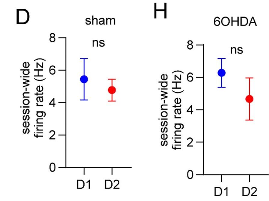
The Reviewer raises a question about the generalizability of the decoder accuracy reported in our study. Fortunately, a comparison between decoder performances on Day 1 and Day 2 datasets does provide insight into this issue. As the Reviewer points out, the classifiers in this study were trained and tested on keypresses performed while practicing a specific sequence (4-1-3-2-4). The study was designed this way as to avoid the impact of interference effects on learning dynamics. The cross-validated performance of classifiers on MEG data collected within the same session was 90.47% overall accuracy (4-class; Figure 3C). We then tested classifier performance on data collected during a separate MEG session conducted approximately 24 hours later (Day 2; see Figure 3 — figure supplement 3). We observed a reduction in overall accuracy rate to 87.11% when tested on MEG data recorded while participants performed the same learned sequence, and 79.44% when they performed several previously unpracticed sequences. Both changes in accuracy are important with regards to the generalizability of our findings. First, 87.11% performance accuracy for the trained sequence data on Day 2 (a reduction of only 3.36%) indicates that the hybrid-space decoder performance is robust over multiple MEG sessions, and thus, robust to variations in SNR across the MEG sensor array caused by small differences in head position between scans. This indicates a substantial advantage over sensor-space decoding approaches. Furthermore, when tested on data from unpracticed sequences, overall performance dropped an additional 7.67%. This difference reflects the performance bias of the classifier for the trained sequence, possibly caused by high-order sequence structure being incorporated into the feature weights. In the future, it will be important to understand in more detail how random or repeated keypress sequence training data impacts overall decoder performance and generalization. We strongly agree with the Reviewer that the issue of generalizability is extremely important and have added a new paragraph to the Discussion in the revised manuscript highlighting the strengths and weaknesses of our study with respect to this issue.
In terms of clinical BCI, one of the potential relevance of the study, as claimed by the authors, it is not clear that the specific time window chosen in the current study (up to 200 msec since key press onset) is really useful. In most cases, clinical BCI would target neural signals with no overt movement execution due to patients' inability to move (e.g., Hochberg et al., 2012). Given the time window, the surprisingly high performance of the current decoder may result from sensory feedback and/or planning of subsequent movement, which may not always be available in the clinical BCI context. Of course, the decoding accuracy is still much higher than chance even when using signal before the key press (as shown in Figure 4 Supplement 2), but it is not immediately clear to me that the authors relate their high decoding accuracy based on post-movement signal to clinical BCI settings.
The Reviewer questions the relevance of the specific window parameters used in the present study for clinical BCI applications, particularly for paretic patients who are unable to produce finger movements or for whom afferent sensory feedback is no longer intact. We strongly agree with the Reviewer that any intended clinical application must carefully consider the specific input feature constraints dictated by the clinical cohort, and in turn impose appropriate and complimentary constraints on classifier parameters that may differ from the ones used in the present study. We now highlight this issue in the Discussion of the revised manuscript and relate our present findings to published clinical BCI work within this context.
One of the important and fascinating claims of the current study is that the "contextualization" of individual finger movements in a trained sequence specifically occurs during short rest periods in very early skill learning, echoing the recent theory of micro-offline learning proposed by the authors' group. Here, I think two points need to be clarified. First, the concept of "contextualization" is kept somewhat blurry throughout the text. It is only at the later part of the Discussion (around line #330 on page 13) that some potential mechanism for the "contextualization" is provided as "what-and-where" binding. Still, it is unclear what "contextualization" actually is in the current data, as the MEG signal analyzed is extracted from 0-200 msec after the keypress. If one thinks something is contextualizing an action, that contextualization should come earlier than the action itself.
The Reviewer requests that we: 1) more clearly define our use of the term “contextualization” and 2) provide the rationale for assessing it over a 200ms window aligned to the KeyDown event. This choice of window parameters means that the MEG activity used in our analysis was coincident with, rather than preceding, the actual keypresses. We define contextualization as the differentiation of representation for the identical movement embedded in different positions of a sequential skill. That is, representations of individual action elements progressively incorporate information about their relationship to the overall sequence structure as the skill is learned. We agree with the Reviewer that this can be appropriately interpreted as “what-and-where” binding. We now incorporate this definition in the Introduction of the revised manuscript as requested.
The window parameters for optimizing accurate decoding individual finger movements were determined using a grid search of the parameter space (a sliding window of variable width between 25-350 ms with 25 ms increments variably aligned from 0 to +100ms with 10ms increments relative to the KeyDown event). This approach generated 140 different temporal windows for each keypress for each participant, with the final parameter selection determined through comparison of the resulting performance between each decoder. Importantly, the decision to optimize for decoding accuracy placed an emphasis on keypress representations characterized by the most consistent and robust features shared across subjects, which in turn maximize statistical power in detecting common learning-related changes. In this case, the optimal window encompassed a 200ms epoch aligned to the KeyDown event (t<sub>0</sub> = 0 ms). We then asked if the representations (i.e. – spatial patterns of combined parcel- and voxel-space activity) of the same digit at two different sequence positions changed with practice within this optimal decoding window. Of course, our findings do not rule out the possibility that contextualization can also be found before or even after this time window, as we did not directly address this issue in the present study. Future work in our lab, as pointed out above, are investigating contextualization within different time windows tailored specifically for assessing sequence skill action planning, execution, evaluation and memory processes.
The second point is that the result provided by the authors is not yet convincing enough to support the claim that "contextualization" occurs during rest. In the original analysis, the authors presented the statistical significance regarding the correlation between the "offline" pattern differentiation and micro-offline skill gain (Figure 5. Supplement 1), as well as the larger "offline" distance than "online" distance (Figure 5B). However, this analysis looks like regressing two variables (monotonically) increasing as a function of the trial. Although some information in this analysis, such as what the independent/dependent variables were or how individual subjects were treated, was missing in the Methods, getting a statistically significant slope seems unsurprising in such a situation. Also, curiously, the same quantitative evidence was not provided for its "online" counterpart, and the authors only briefly mentioned in the text that there was no significant correlation between them. It may be true looking at the data in Figure 5A as the online representation distance looks less monotonically changing, but the classification accuracy presented in Figure 4C, which should reflect similar representational distance, shows a more monotonic increase up to the 11th trial. Further, the ways the "online" and "offline" representation distance was estimated seem to make them not directly comparable. While the "online" distance was computed using all the correct press data within each 10 sec of execution, the "offline" distance is basically computed by only two presses (i.e., the last index_OP5 vs. the first index_OP1 separated by 10 sec of rest). Theoretically, the distance between the neural activity patterns for temporally closer events tends to be closer than that between the patterns for temporally far-apart events. It would be fairer to use the distance between the first index_OP1 vs. the last index_OP5 within an execution period for "online" distance, as well.
The Reviewer suggests that the current data is not enough to show that contextualization occurs during rest and raises two important concerns: 1) the relationship between online contextualization and micro-online gains is not shown, and 2) the online distance was calculated differently from its offline counterpart (i.e. - instead of calculating the distance between last Index<sub>OP5</sub> and first Index<sub>OP1</sub> from a single trial, the distance was calculated for each sequence within a trial and then averaged).
We addressed the first concern by performing individual subject correlations between 1) contextualization changes during rest intervals and micro-offline gains; 2) contextualization changes during practice trials and micro-online gains, and 3) contextualization changes during practice trials and micro-offline gains (Figure 5 – figure supplement 4). We then statistically compared the resulting correlation coefficient distributions and found that within-subject correlations for contextualization changes during rest intervals and micro-offline gains were significantly higher than online contextualization and micro-online gains (t = 3.2827, p = 0.0015) and online contextualization and micro-offline gains (t = 3.7021, p = 5.3013e-04). These results are consistent with our interpretation that micro-offline gains are supported by contextualization changes during the inter-practice rest periods.
With respect to the second concern, we agree with the Reviewer that one limitation of the analysis comparing online versus offline changes in contextualization as presented in the original manuscript, is that it does not eliminate the possibility that any differences could simply be explained by the passage of time (which is smaller for the online analysis compared to the offline analysis). The Reviewer suggests an approach that addresses this issue, which we have now carried out. When quantifying online changes in contextualization from the first Index<sub>OP1</sub> the last Index<sub>OP5</sub> keypress in the same trial we observed no learning-related trend (Figure 5 – figure supplement 5, right panel). Importantly, offline distances were significantly larger than online distances regardless of the measurement approach and neither predicted online learning (Figure 5 – figure supplement 6).
A related concern regarding the control analysis, where individual values for max speed and the degree of online contextualization were compared (Figure 5 Supplement 3), is whether the individual difference is meaningful. If I understood correctly, the optimization of the decoding process (temporal window, feature inclusion/reduction, decoder, etc.) was performed for individual participants, and the same feature extraction was also employed for the analysis of representation distance (i.e., contextualization). If this is the case, the distances are individually differently calculated and they may need to be normalized relative to some stable reference (e.g., 1 vs. 4 or average distance within the control sequence presses) before comparison across the individuals.
The Reviewer makes a good point here. We have now implemented the suggested normalization procedure in the analysis provided in the revised manuscript.
Reviewer #3 (Public review):
Summary:
One goal of this paper is to introduce a new approach for highly accurate decoding of finger movements from human magnetoencephalography data via dimension reduction of a "multiscale, hybrid" feature space. Following this decoding approach, the authors aim to show that early skill learning involves "contextualization" of the neural coding of individual movements, relative to their position in a sequence of consecutive movements. Furthermore, they aim to show that this "contextualization" develops primarily during short rest periods interspersed with skill training and correlates with a performance metric which the authors interpret as an indicator of offline learning.
Strengths:
A clear strength of the paper is the innovative decoding approach, which achieves impressive decoding accuracies via dimension reduction of a "multi-scale, hybrid space". This hybrid-space approach follows the neurobiologically plausible idea of the concurrent distribution of neural coding across local circuits as well as large-scale networks. A further strength of the study is the large number of tested dimension reduction techniques and classifiers (though the manuscript reveals little about the comparison of the latter).
We appreciate the Reviewer’s comments regarding the paper’s strengths.
A simple control analysis based on shuffled class labels could lend further support to this complex decoding approach. As a control analysis that completely rules out any source of overfitting, the authors could test the decoder after shuffling class labels. Following such shuffling, decoding accuracies should drop to chance level for all decoding approaches, including the optimized decoder. This would also provide an estimate of actual chance-level performance (which is informative over and beyond the theoretical chance level). Furthermore, currently, the manuscript does not explain the huge drop in decoding accuracies for the voxel-space decoding (Figure 3B). Finally, the authors' approach to cortical parcellation raises questions regarding the information carried by varying dipole orientations within a parcel (which currently seems to be ignored?) and the implementation of the mean-flipping method (given that there are two dimensions - space and time - what do the authors refer to when they talk about the sign of the "average source", line 477?).
The Reviewer recommends that we: 1) conduct an additional control analysis on classifier performance using shuffled class labels, 2) provide a more detailed explanation regarding the drop in decoding accuracies for the voxel-space decoding following LDA dimensionality reduction (see Fig 3B), and 3) provide additional details on how problems related to dipole solution orientations were addressed in the present study.
In relation to the first point, we have now implemented a random shuffling approach as a control for the classification analyses. The results of this analysis indicated that the chance level accuracy was 22.12% (± SD 9.1%) for individual keypress decoding (4-class classification), and 18.41% (± SD 7.4%) for individual sequence item decoding (5-class classification), irrespective of the input feature set or the type of decoder used. Thus, the decoding accuracy observed with the final model was substantially higher than these chance levels.
Second, please note that the dimensionality of the voxel-space feature set is very high (i.e. – 15684). LDA attempts to map the input features onto a much smaller dimensional space (number of classes – 1; e.g. – 3 dimensions, for 4-class keypress decoding). Given the very high dimension of the voxel-space input features in this case, the resulting mapping exhibits reduced accuracy. Despite this general consideration, please refer to Figure 3—figure supplement 3, where we observe improvement in voxel-space decoder performance when utilizing alternative dimensionality reduction techniques.
The decoders constructed in the present study assess the average spatial patterns across time (as defined by the windowing procedure) in the input feature space. We now provide additional details in the Methods of the revised manuscript pertaining to the parcellation procedure and how the sign ambiguity problem was addressed in our analysis.
Weaknesses:
A clear weakness of the paper lies in the authors' conclusions regarding "contextualization". Several potential confounds, described below, question the neurobiological implications proposed by the authors and provide a simpler explanation of the results. Furthermore, the paper follows the assumption that short breaks result in offline skill learning, while recent evidence, described below, casts doubt on this assumption.
We thank the Reviewer for giving us the opportunity to address these issues in detail (see below).
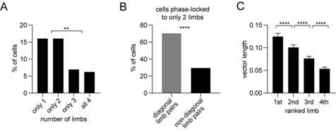
The authors interpret the ordinal position information captured by their decoding approach as a reflection of neural coding dedicated to the local context of a movement (Figure 4). One way to dissociate ordinal position information from information about the moving effectors is to train a classifier on one sequence and test the classifier on other sequences that require the same movements, but in different positions (Kornysheva et al., 2019). In the present study, however, participants trained to repeat a single sequence (4-1-3-2-4). As a result, ordinal position information is potentially confounded by the fixed finger transitions around each of the two critical positions (first and fifth press). Across consecutive correct sequences, the first keypress in a given sequence was always preceded by a movement of the index finger (=last movement of the preceding sequence), and followed by a little finger movement. The last keypress, on the other hand, was always preceded by a ring finger movement, and followed by an index finger movement (=first movement of the next sequence). Figure 4 - Supplement 2 shows that finger identity can be decoded with high accuracy (>70%) across a large time window around the time of the key press, up to at least +/-100 ms (and likely beyond, given that decoding accuracy is still high at the boundaries of the window depicted in that figure). This time window approaches the keypress transition times in this study. Given that distinct finger transitions characterized the first and fifth keypress, the classifier could thus rely on persistent (or "lingering") information from the preceding finger movement, and/or "preparatory" information about the subsequent finger movement, in order to dissociate the first and fifth keypress. Currently, the manuscript provides no evidence that the context information captured by the decoding approach is more than a by-product of temporally extended, and therefore overlapping, but independent neural representations of consecutive keypresses that are executed in close temporal proximity - rather than a neural representation dedicated to context.
Such temporal overlap of consecutive, independent finger representations may also account for the dynamics of "ordinal coding"/"contextualization", i.e., the increase in 2-class decoding accuracy, across Day 1 (Figure 4C). As learning progresses, both tapping speed and the consistency of keypress transition times increase (Figure 1), i.e., consecutive keypresses are closer in time, and more consistently so. As a result, information related to a given keypress is increasingly overlapping in time with information related to the preceding and subsequent keypresses. The authors seem to argue that their regression analysis in Figure 5 - Figure Supplement 3 speaks against any influence of tapping speed on "ordinal coding" (even though that argument is not made explicitly in the manuscript). However, Figure 5 - Figure Supplement 3 shows inter-individual differences in a between-subject analysis (across trials, as in panel A, or separately for each trial, as in panel B), and, therefore, says little about the within-subject dynamics of "ordinal coding" across the experiment. A regression of trial-by-trial "ordinal coding" on trial-by-trial tapping speed (either within-subject or at a group-level, after averaging across subjects) could address this issue. Given the highly similar dynamics of "ordinal coding" on the one hand (Figure 4C), and tapping speed on the other hand (Figure 1B), I would expect a strong relationship between the two in the suggested within-subject (or group-level) regression. Furthermore, learning should increase the number of (consecutively) correct sequences, and, thus, the consistency of finger transitions. Therefore, the increase in 2-class decoding accuracy may simply reflect an increasing overlap in time of increasingly consistent information from consecutive keypresses, which allows the classifier to dissociate the first and fifth keypress more reliably as learning progresses, simply based on the characteristic finger transitions associated with each. In other words, given that the physical context of a given keypress changes as learning progresses - keypresses move closer together in time and are more consistently correct - it seems problematic to conclude that the mental representation of that context changes. To draw that conclusion, the physical context should remain stable (or any changes to the physical context should be controlled for).
The issues raised by Reviewer #3 here are similar to two issues raised by Reviewer #2 above. We agree they must both be carefully considered in any evaluation of our findings.
As both Reviewers pointed out, the classifiers in this study were trained and tested on keypresses performed while practicing a specific sequence (4-1-3-2-4). The study was designed this way as to avoid the impact of interference effects on learning dynamics. The cross-validated performance of classifiers on MEG data collected within the same session was 90.47% overall accuracy (4class; Figure 3C). We then tested classifier performance on data collected during a separate MEG session conducted approximately 24 hours later (Day 2; see Figure 3—supplement 3). We observed a reduction in overall accuracy rate to 87.11% when tested on MEG data recorded while participants performed the same learned sequence, and 79.44% when they performed several previously unpracticed sequences. This classification performance difference of 7.67% when tested on the Day 2 data could reflect the performance bias of the classifier for the trained sequence, possibly caused by mixed information from temporally close keypresses being incorporated into the feature weights.
Along these same lines, both Reviewers also raise the possibility that an increase in “ordinal coding/contextualization” with learning could simply reflect an increase in this mixing effect caused by faster typing speeds as opposed to an actual change in the underlying neural representation. The basic idea is that as correct sequences are generated at higher and higher speeds over training, MEG activity patterns related to the planning, execution, evaluation and memory of individual keypresses overlap more in time. Thus, increased overlap between the “4” and “1” keypresses (at the start of the sequence) and “2” and “4” keypresses (at the end of the sequence) could artefactually increase contextualization distances even if the underlying neural representations for the individual keypresses remain unchanged (assuming this mixing of representations is used by the classifier to differentially tag each index finger press). If this were the case, it follows that such mixing effects reflecting the ordinal sequence structure would also be observable in the distribution of decoder misclassifications. For example, “4” keypresses would be more likely to be misclassified as “1” or “2” keypresses (or vice versa) than as “3” keypresses. The confusion matrices presented in Figures 3C and 4B and Figure 3—figure supplement 3A in the previously submitted manuscript do not show this trend in the distribution of misclassifications across the four fingers.
Following this logic, it’s also possible that if the ordinal coding is largely driven by this mixing effect, the increased overlap between consecutive index finger keypresses during the 4-4 transition marking the end of one sequence and the beginning of the next one could actually mask contextualization-related changes to the underlying neural representations and make them harder to detect. In this case, a decoder tasked with separating individual index finger keypresses into two distinct classes based upon sequence position might show decreased performance with learning as adjacent keypresses overlapped in time with each other to an increasing extent. However, Figure 4C in our previously submitted manuscript does not support this possibility, as the 2-class hybrid classifier displays improved classification performance over early practice trials despite greater temporal overlap.
As noted in the above reply to Reviewer #2, we also conducted a new multivariate regression analysis to directly assess whether the neural representation distance score could be predicted by the 4-1, 2-4 and 4-4 keypress transition times observed for each complete correct sequence (both predictor and response variables were z-score normalized within-subject). The results of this analysis affirmed that the possible alternative explanation put forward by the Reviewer is not supported by our data (Adjusted R<sup>2</sup> = 0.00431; F = 5.62). We now include this new negative control analysis result in the revised manuscript.
Finally, the Reviewer hints that one way to address this issue would be to compare MEG responses before and after learning for sequences typed at a fixed speed. However, given that the speed-accuracy trade-off should improve with learning, a comparison between unlearned and learned skill states would dictate that the skill be evaluated at a very low fixed speed. Essentially, such a design presents the problem that the post-training test is evaluating the representation in the unlearned behavioral state that is not representative of the acquired skill. Thus, this approach would miss most learning effects on a task in which speed is the main learning metrics.
A similar difference in physical context may explain why neural representation distances ("differentiation") differ between rest and practice (Figure 5). The authors define "offline differentiation" by comparing the hybrid space features of the last index finger movement of a trial (ordinal position 5) and the first index finger movement of the next trial (ordinal position 1). However, the latter is not only the first movement in the sequence but also the very first movement in that trial (at least in trials that started with a correct sequence), i.e., not preceded by any recent movement. In contrast, the last index finger of the last correct sequence in the preceding trial includes the characteristic finger transition from the fourth to the fifth movement. Thus, there is more overlapping information arising from the consistent, neighbouring keypresses for the last index finger movement, compared to the first index finger movement of the next trial. A strong difference (larger neural representation distance) between these two movements is, therefore, not surprising, given the task design, and this difference is also expected to increase with learning, given the increase in tapping speed, and the consequent stronger overlap in representations for consecutive keypresses. Furthermore, initiating a new sequence involves pre-planning, while ongoing practice relies on online planning (Ariani et al., eNeuro 2021), i.e., two mental operations that are dissociable at the level of neural representation (Ariani et al., bioRxiv 2023).
The Reviewer argues that the comparison of last finger movement of a trial and the first in the next trial are performed in different circumstances and contexts. This is an important point and one we tend to agree with. For this task, the first sequence in a practice trial is pre-planned before the first keypress is performed. This occurs in a somewhat different context from the sequence iterations that follow, which involve temporally overlapping planning, execution and evaluation processes. The Reviewer is concerned about a difference in the temporal mixing effect issue raised above between the first and last keypresses performed in a trial. Please, note that since neural representations of individual actions are competitively queued during the pre-planning period in a manner that reflects the ordinal structure of the learned sequence (Kornysheva et al., 2019), mixing effects are most likely present also for the first keypress in a trial.
Separately, the Reviewer suggests that contextualization during early learning may reflect preplanning or online planning. This is an interesting proposal. Given the decoding time-window used in this investigation, we cannot dissect separate contributions of planning, memory and sensory feedback to contextualization. Taking advantage of the superior temporal resolution of MEG relative to fMRI tools, work under way in our lab is investigating decoding time-windows more appropriate to address each of these questions.
Given these differences in the physical context and associated mental processes, it is not surprising that "offline differentiation", as defined here, is more pronounced than "online differentiation". For the latter, the authors compared movements that were better matched regarding the presence of consistent preceding and subsequent keypresses (online differentiation was defined as the mean difference between all first vs. last index finger movements during practice). It is unclear why the authors did not follow a similar definition for "online differentiation" as for "micro-online gains" (and, indeed, a definition that is more consistent with their definition of "offline differentiation"), i.e., the difference between the first index finger movement of the first correct sequence during practice, and the last index finger of the last correct sequence. While these two movements are, again, not matched for the presence of neighbouring keypresses (see the argument above), this mismatch would at least be the same across "offline differentiation" and "online differentiation", so they would be more comparable.
This is the same point made earlier by Reviewer #2, and we agree with this assessment. As stated in the response to Reviewer #2 above, we have now carried out quantification of online contextualization using this approach and included it in the revised manuscript. We thank the Reviewer for this suggestion.
A further complication in interpreting the results regarding "contextualization" stems from the visual feedback that participants received during the task. Each keypress generated an asterisk shown above the string on the screen, irrespective of whether the keypress was correct or incorrect. As a result, incorrect (e.g., additional, or missing) keypresses could shift the phase of the visual feedback string (of asterisks) relative to the ordinal position of the current movement in the sequence (e.g., the fifth movement in the sequence could coincide with the presentation of any asterisk in the string, from the first to the fifth). Given that more incorrect keypresses are expected at the start of the experiment, compared to later stages, the consistency in visual feedback position, relative to the ordinal position of the movement in the sequence, increased across the experiment. A better differentiation between the first and the fifth movement with learning could, therefore, simply reflect better decoding of the more consistent visual feedback, based either on the feedback-induced brain response, or feedback-induced eye movements (the study did not include eye tracking). It is not clear why the authors introduced this complicated visual feedback in their task, besides consistency with their previous studies.
We strongly agree with the Reviewer that eye movements related to task engagement are important to rule out as a potential driver of the decoding accuracy or contextualizaton effect. We address this issue above in response to a question raised by Reviewer #1 about the impact of movement related artefacts on our findings.
First, the assumption the Reviewer makes here about the distribution of errors in this task is incorrect. On average across subjects, 2.32% ± 1.48% (mean ± SD) of all keypresses performed were errors, which were evenly distributed across the four possible keypress responses. While errors increased progressively over practice trials, they did so in proportion to the increase in correct keypresses, so that the overall ratio of correct-to-incorrect keypresses remained stable over the training session. Thus, the Reviewer’s assumptions that there is a higher relative frequency of errors in early trials, and a resulting systematic trend phase shift differences between the visual display updates (i.e. – a change in asterisk position above the displayed sequence) and the keypress performed is not substantiated by the data. To the contrary, the asterisk position on the display and the keypress being executed remained highly correlated over the entire training session. We now include a statement about the frequency and distribution of errors in the revised manuscript.
Given this high correlation, we firmly agree with the Reviewer that the issue of eye movement related artefacts is still an important one to address. Fortunately, we did collect eye movement data during the MEG recordings so were able to investigate this. As detailed in the response to Reviewer #1 above, we found that gaze positions and eye-movement velocity time-locked to visual display updates (i.e. – a change in asterisk position above the displayed sequence) did not reflect the asterisk location above chance levels (Overall cross-validated accuracy = 0.21817; see Author response image 1). Furthermore, an inspection of the eye position data revealed that most participants on most trials displayed random walk gaze patterns around a center fixation point, indicating that participants did not attend to the asterisk position on the display. This is consistent with intrinsic generation of the action sequence, and congruent with the fact that the display does not provide explicit feedback related to performance. As pointed out above, a similar real-world example would be manually inputting a long password into a secure online application. In this case, one intrinsically generates the sequence from memory and receives similar feedback about the password sequence position (also provided as asterisks), which is typically ignored by the user.
The minimal participant engagement with the visual display in this explicit sequence learning motor task (which is highly generative in nature) contrasts markedly with behavior observed when reactive responses to stimulus cues are needed in the serial reaction time task (SRTT). This is a crucial difference that must be carefully considered when comparing findings across studies using the two sequence learning tasks.
The authors report a significant correlation between "offline differentiation" and cumulative microoffline gains. However, it would be more informative to correlate trial-by-trial changes in each of the two variables. This would address the question of whether there is a trial-by-trial relation between the degree of "contextualization" and the amount of micro-offline gains - are performance changes (micro-offline gains) less pronounced across rest periods for which the change in "contextualization" is relatively low? Furthermore, is the relationship between micro-offline gains and "offline differentiation" significantly stronger than the relationship between micro-offline gains and "online differentiation"?
In response to a similar issue raised above by Reviewer #2, we now include new analyses comparing correlation magnitudes between (1) “online differentiation” vs micro-online gains, (2) “online differentiation” vs micro-offline gains and (3) “offline differentiation” and micro-offline gains (see Figure 5 – figure supplement 4, 5 and 6). These new analyses and results have been added to the revised manuscript. Once again, we thank both Reviewers for this suggestion.
The authors follow the assumption that micro-offline gains reflect offline learning.
We disagree with this statement. The original (Bonstrup et al., 2019) paper clearly states that micro-offline gains do not necessarily reflect offline learning in some cases and must be carefully interpreted based upon the behavioral context within which they are observed. Further, the paper lays out the conditions under which one can have confidence that micro-offline gains reflect offline learning. In fact, the excellent meta-analysis of (Pan & Rickard, 2015), which re-interprets the benefits of sleep in overnight skill consolidation from a “reactive inhibition” perspective, was a crucial resource in the experimental design of our initial study (Bonstrup et al., 2019), as well as in all our subsequent work. Pan & Rickard state:
“Empirically, reactive inhibition refers to performance worsening that can accumulate during a period of continuous training (Hull, 1943 . It tends to dissipate, at least in part, when brief breaks are inserted between blocks of training. If there are multiple performance-break cycles over a training session, as in the motor sequence literature, performance can exhibit a scalloped effect, worsening during each uninterrupted performance block but improving across blocks(Brawn et al., 2010; Rickard et al., 2008 . Rickard, Cai, Rieth, Jones, and Ard (2008 and Brawn, Fenn, Nusbaum, and Margoliash (2010 (Brawn et al., 2010; Rickard et al., 2008 demonstrated highly robust scalloped reactive inhibition effects using the commonly employed 30 s–30 s performance break cycle, as shown for Rickard et al.’s (2008 massed practice sleep group in Figure 2. The scalloped effect is evident for that group after the first few 30 s blocks of each session. The absence of the scalloped effect during the first few blocks of training in the massed group suggests that rapid learning during that period masks any reactive inhibition effect.”
Crucially, Pan & Rickard make several concrete recommendations for reducing the impact of the reactive inhibition confound on offline learning studies. One of these recommendations was to reduce practice times to 10s (most prior sequence learning studies up until that point had employed 30s long practice trials). They state:
“The traditional design involving 30 s-30 s performance break cycles should be abandoned given the evidence that it results in a reactive inhibition confound, and alternative designs with reduced performance duration per block used instead (Pan & Rickard, 2015 . One promising possibility is to switch to 10 s performance durations for each performance-break cycle Instead (Pan & Rickard, 2015 . That design appears sufficient to eliminate at least the majority of the reactive inhibition effect (Brawn et al., 2010; Rickard et al., 2008 .”
We mindfully incorporated recommendations from (Pan & Rickard, 2015) into our own study designs including 1) utilizing 10s practice trials and 2) constraining our analysis of micro-offline gains to early learning trials (where performance monotonically increases and 95% of overall performance gains occur), which are prior to the emergence of the “scalloped” performance dynamics that are strongly linked to reactive inhibition effects.
However, there is no direct evidence in the literature that micro-offline gains really result from offline learning, i.e., an improvement in skill level.
We strongly disagree with the Reviewer’s assertion that “there is no direct evidence in the literature that micro-offline gains really result from offline learning, i.e., an improvement in skill level.” The initial (Bonstrup et al., 2019) report was followed up by a large online crowd-sourcing study (Bonstrup et al., 2020). This second (and much larger) study provided several additional important findings supporting our interpretation of micro-offline gains in cases where the important behavioral conditions clarified above were met (see Author response image 4 below for further details on these conditions).
Author response image 4.
This Figure shows that micro-offline gains o ser ed in learning and nonlearning contexts are attri uted to different underl ing causes. Micro-offline and online changes relative to overall trial-by-trial learning. This figure is based on data from (Bonstrup et al., 2019). During early learning, micro-offline gains (red bars) closely track trial-by-trial performance gains (green line with open circle markers), with minimal contribution from micro-online gains (blue bars). The stated conclusion in Bönstrup et al. (2019) is that micro-offline gains only during this Early Learning stage reflect rapid memory consolidation (see also (Bonstrup et al., 2020)). After early learning, about practice trial 11, skill plateaus. This plateau skill period is characterized by a striking emergence of coupled (and relatively stable) micro-online drops and micro-offline increases. Bönstrup et al. (2019) as well as others in the literature (Brooks et al., 2024; Gupta & Rickard, 2022; Florencia Jacobacci et al., 2020), argue that micro-offline gains during the plateau period likely reflect recovery from inhibitory performance factors such as reactive inhibition or fatigue, and thus must be excluded from analyses relating micro-offline gains to skill learning. The Non-repeating groups in Experiments 3 and 4 from Das et al. (2024) suffer from a lack of consideration of these known confounds (end of Fig legend).
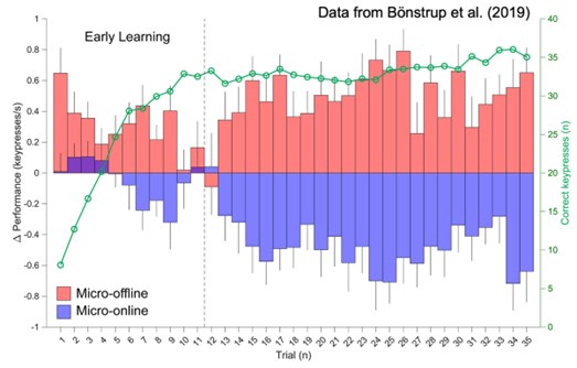
Evidence documented in that paper (Bonstrup et al., 2020) showed that micro-offline gains during early skill learning were: 1) replicable and generalized to subjects learning the task in their daily living environment (n=389); 2) equivalent when significantly shortening practice period duration, thus confirming that they are not a result of recovery from performance fatigue (n=118); 3) reduced (along with learning rates) by retroactive interference applied immediately after each practice period relative to interference applied after passage of time (n=373), indicating stabilization of the motor memory at a microscale of several seconds consistent with rapid consolidation; and 4) not modified by random termination of the practice periods, ruling out a contribution of predictive motor slowing (N = 71) (Bonstrup et al., 2020). Altogether, our findings were strongly consistent with the interpretation that micro-offline gains reflect memory consolidation supporting early skill learning. This is precisely the portion of the learning curve (Pan & Rickard, 2015) refer to when they state “…rapid learning during that period masks any reactive inhibition effect”.
This interpretation is further supported by brain imaging evidence linking known memory-related networks and consolidation mechanisms to micro-offline gains. First, we reported that the density of fast hippocampo-neocortical skill memory replay events increases approximately three-fold during early learning inter-practice rest periods with the density explaining differences in the magnitude of micro-offline gains across subjects (Buch et al., 2021). Second, Jacobacci et al. (2020) independently reproduced our original behavioral findings and reported BOLD fMRI changes in the hippocampus and precuneus (regions also identified in our MEG study (Buch et al., 2021)) linked to micro-offline gains during early skill learning. These functional changes were coupled with rapid alterations in brain microstructure in the order of minutes, suggesting that the same network that operates during rest periods of early learning undergoes structural plasticity over several minutes following practice (Deleglise et al., 2023). Crucial to this point, Chen et al. (2024) and Sjøgård et al (2024) provided direct evidence from intracranial EEG in humans linking sharp-wave ripple density during rest periods (which are known markers for neural replay (Buzsaki, 2015)) in the human hippocampus (80-120 Hz) to micro-offline gains during early skill learning.
Thus, there is now substantial converging evidence in humans across different indirect noninvasive and direct invasive recording techniques linking hippocampal activity, neural replay dynamics and offline performance gains in skill learning.
On the contrary, recent evidence questions this interpretation (Gupta & Rickard, npj Sci Learn 2022; Gupta & Rickard, Sci Rep 2024; Das et al., bioRxiv 2024). Instead, there is evidence that micro-offline gains are transient performance benefits that emerge when participants train with breaks, compared to participants who train without breaks, however, these benefits vanish within seconds after training if both groups of participants perform under comparable conditions (Das et al., bioRxiv 2024).
The recent work of (Gupta & Rickard, 2022, 2024) does not present any data that directly opposes our finding that early skill learning (Bonstrup et al., 2019) is expressed as micro-offline gains during rest breaks. These studies are an extension of the Rickard et al (2008) paper that employed a massed (30s practice followed by 30s breaks) vs spaced (10s practice followed by 10s breaks) experimental design to assess if recovery from reactive inhibition effects could account for performance gains measured after several minutes or hours. Gupta & Rickard (2022) added two additional groups (30s practice/10s break and 10s practice/10s break as used in the work from our group). The primary aim of the study was to assess whether it was more likely that changes in performance when retested 5 minutes after skill training (consisting of 12 practice trials for the massed groups and 36 practice trials for the spaced groups) had ended reflected memory consolidation effects or recovery from reactive inhibition effects. The Gupta & Rickard (2024) follow-up paper employed a similar design with the primary difference being that participants performed a fixed number of sequences on each trial as opposed to trials lasting a fixed duration. This was done to facilitate the fitting of a quantitative statistical model to the data.
To reiterate, neither study included any analysis of micro-online or micro-offline gains and did not include any comparison focused on skill gains during early learning trials (only at retest 5 min later). Instead, Gupta & Rickard (2022), reported evidence for reactive inhibition effects for all groups over much longer training periods than early learning. In fact, we reported the same findings for trials following the early learning period in our original 2019 paper (Bonstrup et al., 2019) (Author response image 4). Please, note that we also reported that cumulative microoffline gains over early learning did not correlate with overnight offline consolidation measured 24 hours later (Bonstrup et al., 2019) (see the Results section and further elaboration in the Discussion). We interpreted these findings as indicative that the mechanisms underlying offline gains over the micro-scale of seconds during early skill learning versus over minutes or hours very likely differ.
In the recent preprint from (Das et al., 2024), the authors make the strong claim that “micro-offline gains during early learning do not reflect offline learning” which is not supported by their own data. The authors hypothesize that if “micro-offline gains represent offline learning, participants should reach higher skill levels when training with breaks, compared to training without breaks”. The study utilizes a spaced vs. massed practice groups between-subjects design inspired by the reactive inhibition work from Rickard and others to test this hypothesis.
Crucially, their design incorporates only a small fraction of the training used in other investigations to evaluate early skill learning (Bonstrup et al., 2020; Bonstrup et al., 2019; Brooks et al., 2024; Buch et al., 2021; Deleglise et al., 2023; F. Jacobacci et al., 2020; Mylonas et al., 2024). A direct comparison between the practice schedule designs for the spaced and massed groups in Das et al., and the training schedule all participants experienced in the original Bönstrup et al. (2019) paper highlights this issue as well as several others (Author response image 5):
Author response image 5.
This figure shows (A) Comparison of Das et al. Spaced & Massed group training session designs, and the training session design from the original (Bonstrup et al., 2019) paper. Similar to the approach taken by Das et al., all practice is visualized as 10-second practice trials with a variable number (either 0, 1 or 30) of 10-second-long inter-practice rest intervals to allow for direct comparisons between designs. The two key takeaways from this comparison are that (1) the intervention differences (i.e. – practice schedules) between the Massed and Spaced groups from the Das et al. report are extremely small (less than 12% of the overall session schedule) (gaps in the red shaded area) and (2) the overall amount of practice is much less than compared to the design from the original Bönstrup report (Bonstrup et al., 2019) (which has been utilized in several subsequent studies). (B) Group-level learning curve data from Bönstrup et al. (2019) (Bonstrup et al., 2019) is used to estimate the performance range accounted for by the equivalent periods covering Test 1, Training 1 and Test 2 from Das et al (2024). Note that the intervention in the Das et al. study is limited to a period covering less than 50% of the overall learning range (end of figure legend).
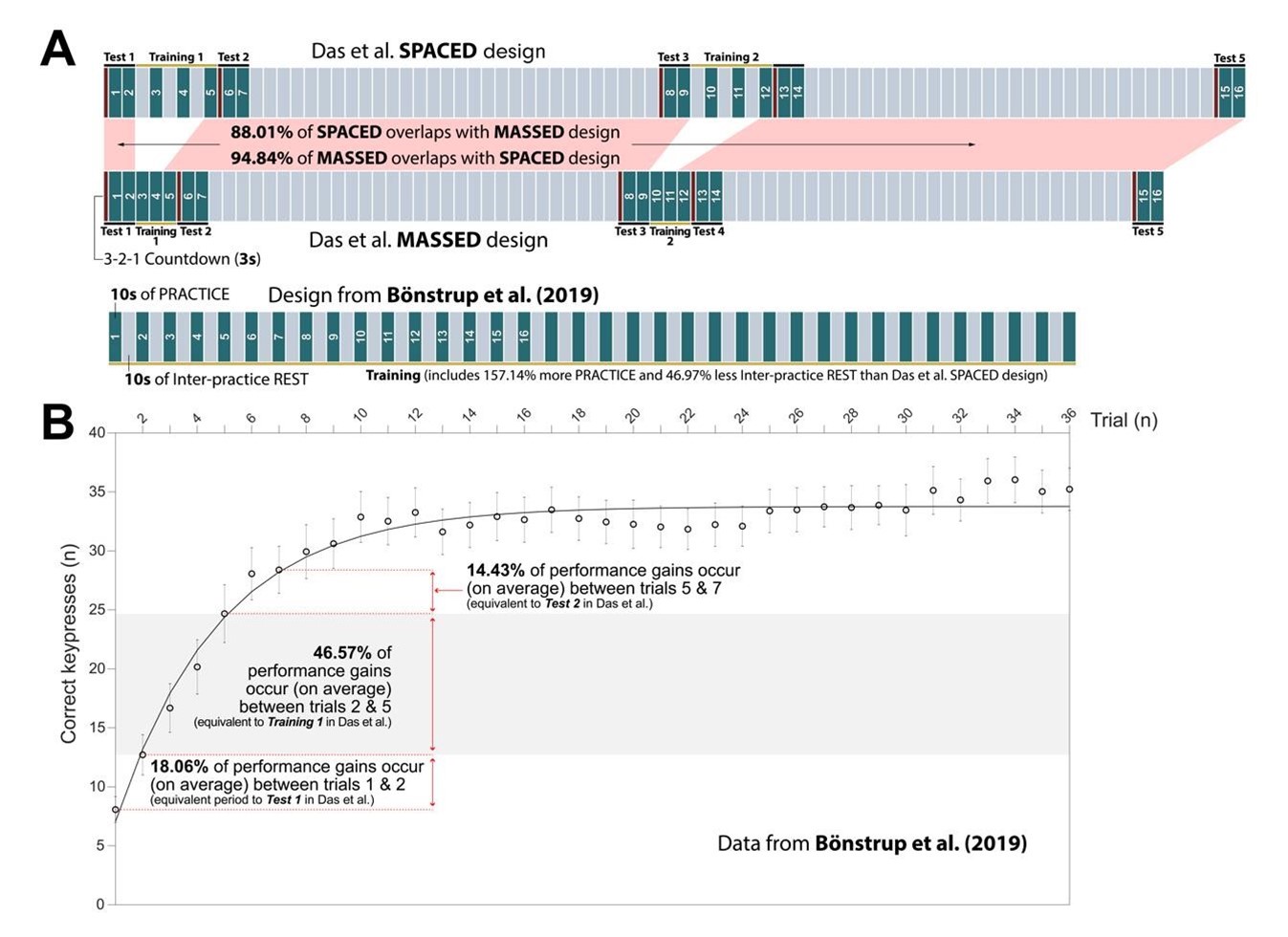
Participants in the original (Bonstrup et al., 2019) experienced 157.14% more practice time and 46.97% less inter-practice rest time than the Spaced group in the Das et al. study (Author response image 5). Thus, the overall amount of practice and rest differ substantially between studies, with much more limited training occurring for participants in Das et al.
In addition, the training interventions (i.e. – the practice schedule differences between the Spaced and Massed groups) were designed in a manner that minimized any chance of effectively testing their hypothesis. First, the interventions were applied over an extremely short period relative to the length of the total training session (5% and 12% of the total training session for Massed and Spaced groups, respectively; see gaps in the red shaded area in Author response image 5). Second, the intervention was applied during a period in which only half of the known total learning occurs. Specifically, we know from Bönstrup et al. (2019) that only 46.57% of the total performance gains occur in the practice interval covered by Das et al Training 1 intervention. Thus, early skill learning as evaluated by multiple groups (Bonstrup et al., 2020; Bonstrup et al., 2019; Brooks et al., 2024; Buch et al., 2021; Deleglise et al., 2023; F. Jacobacci et al., 2020; Mylonas et al., 2024), is in the Das et al experiment amputated to about half.
Furthermore, a substantial amount of learning takes place during Das et al’s Test 1 and Test 2 periods (32.49% of total gains combined). The fact that substantial learning is known to occur over both the Test 1 (18.06%) and Test 2 (14.43%) intervals presents a fundamental problem described by Pan and Rickard (Pan & Rickard, 2015). They reported that averaging over intervals where substantial performance gains occur (i.e. – performance is not stable) inject crucial artefacts into analyses of skill learning:
“A large amount of averaging has the advantage of yielding more precise estimates of each subject’s pretest and posttest scores and hence more statistical power to detect a performance gain. However, calculation of gain scores using that strategy runs the risk that learning that occurs during the pretest and (or posttest periods (i.e., online learning is incorporated into the gain score (Rickard et al., 2008; Robertson et al., 2004 .”
The above statement indicates that the Test 1 and Test 2 performance scores from Das et al. (2024) are substantially contaminated by the learning rate within these intervals. This is particularly problematic if the intervention design results in different Test 2 learning rates between the two groups. This in fact, is apparent in their data (Figure 1C,E of the Das et al., 2024 preprint) as the Test 2 learning rate for the Spaced group is negative (indicating a unique interference effect observable only for this group). Specifically, the Massed group continues to show an increase in performance during Test 2 and 4 relative to the last 10 seconds of practice during Training 1 and 2, respectively, while the Spaced group displays a marked decrease. This post-training performance decrease for the Spaced group is in stark contrast to the monotonic performance increases observed for both groups at all other time-points. One possible cause could be related to the structure of the Test intervals, which include 20 seconds of uninterrupted practice. For the Spaced group, this effectively is a switch to a Massed practice environment (i.e., two 10-secondlong practice trials merged into one long trial), which interferes with greater Training 1 interval gains observed for the Space group. Interestingly, when statistical comparisons between the groups are made at the time-points when the intervention is present (Figure 1E) then the stated hypothesis, “If micro-offline gains represent offline learning, participants should reach higher skill levels when training with breaks, compared to training without breaks”, is confirmed.
In summary, the experimental design and analyses used by Das et al does not contradict the view that early skill learning is expressed as micro-offline gains during rest breaks. The data presented by Gupta and Rickard (2022, 2024) and Das et al. (2024) is in many ways more confirmatory of the constraints employed by our group and others with respect to experimental design, analysis and interpretation of study findings, rather than contradictory. Still, it does highlight a limitation of the current micro-online/offline framework, which was originally only intended to be applied to early skill learning over spaced practice schedules when reactive inhibition effects are minimized (Bonstrup et al., 2019; Pan & Rickard, 2015). Extrapolation of this current framework to postplateau performance periods, longer timespans, or non-learning situations (e.g. – the Nonrepeating groups from Das et al. (2024)), when reactive inhibition plays a more substantive role, is not warranted. Ultimately, it will be important to develop new paradigms allowing one to independently estimate the different coincident or antagonistic features (e.g. - memory consolidation, planning, working memory and reactive inhibition) contributing to micro-online and micro-offline gains during and after early skill learning within a unifying framework.
Recommendations for the authors:
Reviewer #1 (Recommendations for the authors):
(1) I found Figure 2B too small to be useful, as the actual elements of the cells are very hard to read.
We have removed the grid colormap panel (top-right) from Figure 2B. All of this colormap data is actually a subset of data presented in Figure 2 – figure supplement 1, so can still be found there.
Reviewer #2 (Recommendations for the authors):
(1) Related to the first point in my concerns, I would suggest the authors compare decoding accuracy between correct presses followed by correct vs. incorrect presses. This would clarify if the decoder is actually taking the MEG signal for subsequent press into account. I would also suggest the authors use pre-movement MEG features and post-movement features with shorter windows and compare each result with the results for the original post-movement MEG feature with a longer window.
The present study does not contain enough errors to perform the analysis proposed by the Reviewer. As noted above, we did re-examine our data and now report a new control regression analysis, all of which indicate that the proximity between keypresses does not explain contextualization effects.
(2) I was several times confused by the author's use of "neural representation of an action" or "sequence action representations" in understanding whether these terms refer to representation on the level of whole-brain, region (as defined by the specific parcellation used), or voxels. In fact, what is submitted to the decoder is some complicated whole-brain MEG feature (i.e., the "neural representation"), which is a hybrid of voxel and parcel features that is further dimension-reduced and not immediately interpretable. Clarifying this point early in the text and possibly using some more sensible terms, such as adding "brain-wise" before the "sequence action representation", would be the most helpful for the readers.
We now clarified this terminology in the revised manuscript.
(3) Although comparing many different ways in feature selection/reduction, time window selection, and decoder types is undoubtedly a meticulous work, the current version of the manuscript seems still lacking some explanation about the details of these methodological choices, like which decoding method was actually used to report the accuracy, whether or not different decoding methods were chosen for individual participants' data, how training data was selected (is it all of the correct presses in Day 1 data?), whether the frequency power or signal amplitude was used, and so on. I would highly appreciate these additional details in the Methods section.
The reported accuracies were based on linear discriminant analysis classifier. A comparison of different decoders (Figure 3 – figure supplement 4) shows LDA was the optimal choice.
Whether or not different decoding methods were chosen for individual participants' data
We selected the same decoder (LDA) performance to report the final accuracy.
How training data was selected (is it all of the correct presses in Day 1 data?),
Decoder training was conducted as a randomized split of the data (all correct keypresses of Day 1) into training (90%) and test (10%) samples for 8 iterations.
Whether the frequency power or signal amplitude was used
Signal amplitude was used for feature calculation.
(4) In terms of the Methods, please consider adding some references about the 'F1 score', the 'feature importance score,' and the 'MRMR-based feature ranking,' as the main readers of the current paper would not be from the machine learning community. Also, why did the LDA dimensionality reduction reduce accuracy specifically for the voxel feature?
We have now added the following statements to the Methods section that provide more detailed descriptions and references for these metrics:
“The F1 score, defined as the harmonic mean of the precision (percentage of true predictions that are actually true positive) and recall (percentage of true positives that were correctly predicted as true) scores, was used as a comprehensive metric for all one-versus-all keypress state decoders to assess class-wise performance that accounts for both false-positive and false-negative prediction tendencies [REF]. A weighted mean F1 score was then computed across all classes to assess the overall prediction performance of the multi-class model.”
and
“Feature Importance Scores
The relative contribution of source-space voxels and parcels to decoding performance (i.e. – feature importance score) was calculated using minimum redundant maximum relevance (MRMR) and highlighted in topography plots. MRMR, an approach that combines both relevance and redundancy metrics, ranked individual features based upon their significance to the target variable (i.e. – keypress state identity) prediction accuracy and their non-redundancy with other features.”
As stated in the Reviewer responses above, the dimensionality of the voxel-space feature set is very high (i.e. – 15684). LDA attempts to map the input features onto a much smaller dimensional space (number of classes-1; e.g. – 3 dimensions for 4-class keypress decoding). It is likely that the reduction in accuracy observed only for the voxel-space feature was due to the loss of relevant information during the mapping process that resulted in reduced accuracy. This reduction in accuracy for voxel-space decoding was specific to LDA. Figure 3—figure supplement 3 shows that voxel-space decoder performance actually improved when utilizing alternative dimensionality reduction techniques.
(5) Paragraph 9, lines #139-142: "Notably, decoding associated with index finger keypresses (executed at two different ordinal positions in the sequence) exhibited the highest number of misclassifications of all digits (N = 141 or 47.5% of all decoding errors; Figure 3C), raising the hypothesis that the same action could be differentially represented when executed at different learning state or sequence context locations."
This does not seem to be a fair comparison, as the index finger appears twice as many as the other fingers do in the sequence. To claim this, proper statistical analysis needs to be done taking this difference into account.
We thank the Reviewer for bringing this issue to our attention. We have now corrected this comparison to evaluate relative false negative and false positive rates between individual keypress state decoders, and have revised this statement in the manuscript as follows:
“Notably, decoding of index finger keypresses (executed at two different ordinal positions in the sequence) exhibited the highest false negative (0.116 per keypress) and false positive (0.043 per keypress) misclassification rates compared with all other digits (false negative rate range = [0.067 0.114]; false positive rate range = [0.020 0.037]; Figure 3C), raising the hypothesis that the same action could be differentially represented when executed within different contexts (i.e. - different learning states or sequence locations).”
(6) Finally, the authors could consider acknowledging in the Discussion that the contribution of micro-offline learning to genuine skill learning is still under debate (e.g., Gupta and Rickard, 2023; 2024; Das et al., bioRxiv, 2024).
We have added a paragraph in the Discussion that addresses this point.
Reviewer #3 (Recommendations for the authors):
In addition to the additional analyses suggested in the public review, I have the following suggestions/questions:
(1) Given that the authors introduce a new decoding approach, it would be very helpful for readers to see a distribution of window sizes and window onsets eventually used across individuals, at least for the optimized decoder.
We have now included a new supplemental figure (Figure 4 – figure Supplement 2) that provides this information.
(2) Please explain in detail how you arrived at the (interpolated?) group-level plot shown in Figure 1B, starting from the discrete single-trial keypress transition times. Also, please specify what the shading shows.
Instantaneous correct sequence speed (skill measure) was quantified as the inverse of time (in seconds) required to complete a single iteration of a correctly generated full 5-item sequence. Individual keypress responses were labeled as members of correct sequences if they occurred within a 5-item response pattern matching any possible circular shifts of the 5-item sequence displayed on the monitor (41324). This approach allowed us to quantify a measure of skill within each practice trial at the resolution of individual keypresses. The dark line indicates the group mean performance dynamics for each trial. The shaded region indicates the 95% confidence limit of the mean (see Methods).
(3) Similarly, please explain how you arrived at the group-level plot shown in Figure 1C. What are the different colored lines (rows) within each trial? How exactly did the authors reach the conclusion that KTT variability stabilizes by trial 6?
Figure 1C provides additional information to the correct sequence speed measure above, as it also tracks individual transition speed composition over learning. Figure 1C, thus, represents both changes in overall correct sequence speed dynamics (indicated by the overall narrowing of the horizontal speed lines moving from top to bottom) and the underlying composition of the individual transition patterns within and across trials. The coloring of the lines is a shading convention used to discriminate between different keypress transitions. These curves were sampled with 1ms resolution, as in Figure 1B. Addressing the underlying keypress transition patterns requires within-subject normalization before averaging across subjects. The distribution of KTTs was normalized to the median correct sequence time for each participant and centered on the mid-point for each full sequence iteration during early learning.
(4) Maybe I missed it, but it was not clear to me which of the tested classifiers was eventually used. Or was that individualized as well? More generally, a comparison of the different classifiers would be helpful, similar to the comparison of dimension reduction techniques.
We have now included a new supplemental figure that provides this information.
(5) Please add df and effect sizes to all statistics.
Done.
(6) Please explain in more detail your power calculation.
The study was powered to determine the minimum sample size needed to detect a significant change in skill performance following training using a one-sample t-test (two-sided; alpha = 0.05; 95% statistical power; Cohen’s D effect size = 0.8115 calculated from previously acquired data in our lab). The calculated minimum sample size was 22. The included study sample size (n = 27) exceeded this minimum.
This information is now included in the revised manuscript.
(7) The cut-off for the high-pass filter is unusually high and seems risky in terms of potential signal distortions (de Cheveigne, Neuron 2019). Why did the authors choose such a high cut-off?
The 1Hz high-pass cut-off frequency for the 1-150Hz band-pass filter applied to the continuous raw MEG data during preprocessing has been used in multiple previous MEG publications (Barratt et al., 2018; Brookes et al., 2012; Higgins et al., 2021; Seedat et al., 2020; Vidaurre et al., 2018).
(8) "Furthermore, the magnitude of offline contextualization predicted skill gains while online contextualization did not", lines 336/337 - where is that analysis?
Additional details pertaining to this analysis are now provided in the Results section (Figure 5 – figure supplement 4).
(9) How were feature importance scores computed?
We have now added a new subheading in the Methods section with a more detailed description of how feature importance scores were computed.
(10) Please add x and y ticks plus tick labels to Figure 5 - Figure Supplement 3, panel A
Done
(11) Line 369, what does "comparable" mean in this context?
The sentence in the “Study Participants” part of the Methods section referred to here has now been revised for clarity.
(12) In lines 496/497, please specify what t=0 means (KeyDown event, I guess?).
Yes, the KeyDown event occurs at t = 0. This has now been clarified in the revised manuscript.
(13) Please specify consistent boundaries between alpha- and beta-bands (they are currently not consistent in the Results vs. Methods (14/15 Hz or 15/16 Hz)).
We thank the Reviewer for alerting us to this discrepancy caused by a typographic error in the Methods. We have now corrected this so that the alpha (8-14 Hz) and beta-band (15-24 Hz) frequency limits are described consistently throughout the revised manuscript.
References
Albouy, G., Fogel, S., King, B. R., Laventure, S., Benali, H., Karni, A., Carrier, J., Robertson, E. M., & Doyon, J. (2015). Maintaining vs. enhancing motor sequence memories: respective roles of striatal and hippocampal systems. Neuroimage, 108, 423-434. https://doi.org/10.1016/j.neuroimage.2014.12.049
Albouy, G., King, B. R., Maquet, P., & Doyon, J. (2013). Hippocampus and striatum: dynamics and interaction during acquisition and sleep-related motor sequence memory consolidation. Hippocampus, 23(11), 985-1004. https://doi.org/10.1002/hipo.22183 Albouy, G., Sterpenich, V., Vandewalle, G., Darsaud, A., Gais, S., Rauchs, G., Desseilles, M., Boly, M., Dang-Vu, T., Balteau, E., Degueldre, C., Phillips, C., Luxen, A., & Maquet, P. (2012). Neural correlates of performance variability during motor sequence acquisition. NeuroImage, 60(1), 324-331. https://doi.org/10.1016/j.neuroimage.2011.12.049
Andersen, R. A., & Buneo, C. A. (2002). Intentional maps in posterior parietal cortex. Annu Rev Neurosci, 25, 189-220. https://doi.org/10.1146/annurev.neuro.25.112701.142922 112701.142922 [pii]
Ashe, J., Lungu, O. V., Basford, A. T., & Lu, X. (2006). Cortical control of motor sequences. Curr Opin Neurobiol, 16(2), 213-221. http://www.ncbi.nlm.nih.gov/entrez/query.fcgi?cmd=Retrieve&db=PubMed&dopt=Citati on&list_uids=16563734
Bansal, A. K., Vargas-Irwin, C. E., Truccolo, W., & Donoghue, J. P. (2011). Relationships among low-frequency local field potentials, spiking activity, and three-dimensional reach and grasp kinematics in primary motor and ventral premotor cortices. J Neurophysiol, 105(4), 1603-1619. https://doi.org/10.1152/jn.00532.2010
Barratt, E. L., Francis, S. T., Morris, P. G., & Brookes, M. J. (2018). Mapping the topological organisation of beta oscillations in motor cortex using MEG. NeuroImage, 181, 831-844. https://doi.org/10.1016/j.neuroimage.2018.06.041
Bassett, D. S., Wymbs, N. F., Porter, M. A., Mucha, P. J., Carlson, J. M., & Grafton, S. T. (2011). Dynamic reconfiguration of human brain networks during learning. Proc Natl Acad Sci U S A, 108(18), 7641-7646. https://doi.org/10.1073/pnas.1018985108
Battaglia-Mayer, A., & Caminiti, R. (2019). Corticocortical Systems Underlying High-Order Motor Control. J Neurosci, 39(23), 4404-4421. https://doi.org/10.1523/JNEUROSCI.2094-18.2019
Berlot, E., Popp, N. J., & Diedrichsen, J. (2020). A critical re-evaluation of fMRI signatures of motor sequence learning. Elife, 9. https://doi.org/10.7554/eLife.55241
Bonstrup, M., Iturrate, I., Hebart, M. N., Censor, N., & Cohen, L. G. (2020). Mechanisms of offline motor learning at a microscale of seconds in large-scale crowdsourced data. NPJ Sci Learn, 5, 7. https://doi.org/10.1038/s41539-020-0066-9
Bonstrup, M., Iturrate, I., Thompson, R., Cruciani, G., Censor, N., & Cohen, L. G. (2019). A Rapid Form of Offline Consolidation in Skill Learning. Curr Biol, 29(8), 1346-1351 e1344. https://doi.org/10.1016/j.cub.2019.02.049
Brawn, T. P., Fenn, K. M., Nusbaum, H. C., & Margoliash, D. (2010). Consolidating the effects of waking and sleep on motor-sequence learning. J Neurosci, 30(42), 13977-13982. https://doi.org/10.1523/JNEUROSCI.3295-10.2010
Brookes, M. J., Woolrich, M. W., & Barnes, G. R. (2012). Measuring functional connectivity in MEG: a multivariate approach insensitive to linear source leakage. NeuroImage, 63(2), 910-920. https://doi.org/10.1016/j.neuroimage.2012.03.048
Brooks, E., Wallis, S., Hendrikse, J., & Coxon, J. (2024). Micro-consolidation occurs when learning an implicit motor sequence, but is not influenced by HIIT exercise. NPJ Sci Learn, 9(1), 23. https://doi.org/10.1038/s41539-024-00238-6
Buch, E. R., Claudino, L., Quentin, R., Bonstrup, M., & Cohen, L. G. (2021). Consolidation of human skill linked to waking hippocampo-neocortical replay. Cell Rep, 35(10), 109193. https://doi.org/10.1016/j.celrep.2021.109193
Buneo, C. A., & Andersen, R. A. (2006). The posterior parietal cortex: sensorimotor interface for the planning and online control of visually guided movements. Neuropsychologia, 44(13), 2594-2606. https://doi.org/10.1016/j.neuropsychologia.2005.10.011
Buzsaki, G. (2015). Hippocampal sharp wave-ripple: A cognitive biomarker for episodic memory and planning. Hippocampus, 25(10), 1073-1188. https://doi.org/10.1002/hipo.22488
Chen, P.-C., Stritzelberger, J., Walther, K., Hamer, H., & Staresina, B. P. (2024). Hippocampal ripples during offline periods predict human motor sequence learning. bioRxiv, 2024.2010.2006.614680. https://doi.org/10.1101/2024.10.06.614680
Churchland, M. M., Cunningham, J. P., Kaufman, M. T., Foster, J. D., Nuyujukian, P., Ryu, S. I., & Shenoy, K. V. (2012). Neural population dynamics during reaching. Nature, 487(7405), 51-56. https://doi.org/10.1038/nature11129
Classen, J., Liepert, J., Wise, S. P., Hallett, M., & Cohen, L. G. (1998). Rapid plasticity of human cortical movement representation induced by practice. J Neurophysiol, 79(2), 1117-1123. http://www.ncbi.nlm.nih.gov/entrez/query.fcgi?cmd=Retrieve&db=PubMed&dopt=Citati on&list_uids=9463469
Colclough, G. L., Brookes, M. J., Smith, S. M., & Woolrich, M. W. (2015). A symmetric multivariate leakage correction for MEG connectomes. NeuroImage, 117, 439-448. https://doi.org/10.1016/j.neuroimage.2015.03.071
Colclough, G. L., Woolrich, M. W., Tewarie, P. K., Brookes, M. J., Quinn, A. J., & Smith, S. M. (2016). How reliable are MEG resting-state connectivity metrics? NeuroImage, 138, 284-293. https://doi.org/10.1016/j.neuroimage.2016.05.070
Das, A., Karagiorgis, A., Diedrichsen, J., Stenner, M.-P., & Azanon, E. (2024). “Micro-offline gains” convey no benefit for motor skill learning. bioRxiv, 2024.2007.2011.602795. https://doi.org/10.1101/2024.07.11.602795
Deleglise, A., Donnelly-Kehoe, P. A., Yeffal, A., Jacobacci, F., Jovicich, J., Amaro, E., Jr., Armony, J. L., Doyon, J., & Della-Maggiore, V. (2023). Human motor sequence learning drives transient changes in network topology and hippocampal connectivity early during memory consolidation. Cereb Cortex, 33(10), 6120-6131. https://doi.org/10.1093/cercor/bhac489
Doyon, J., Bellec, P., Amsel, R., Penhune, V., Monchi, O., Carrier, J., Lehéricy, S., & Benali, H. (2009). Contributions of the basal ganglia and functionally related brain structures to motor learning. [Review]. Behavioural brain research, 199(1), 61-75. https://doi.org/10.1016/j.bbr.2008.11.012
Doyon, J., Song, A. W., Karni, A., Lalonde, F., Adams, M. M., & Ungerleider, L. G. (2002). Experience-dependent changes in cerebellar contributions to motor sequence learning. Proc Natl Acad Sci U S A, 99(2), 1017-1022. http://www.ncbi.nlm.nih.gov/entrez/query.fcgi?cmd=Retrieve&db=PubMed&dopt=Citati on&list_uids=11805340
Euston, D. R., Gruber, A. J., & McNaughton, B. L. (2012). The role of medial prefrontal cortex in memory and decision making. Neuron, 76(6), 1057-1070. https://doi.org/10.1016/j.neuron.2012.12.002
Euston, D. R., Tatsuno, M., & McNaughton, B. L. (2007). Fast-forward playback of recent memory sequences in prefrontal cortex during sleep. Science, 318(5853), 1147-1150. https://doi.org/10.1126/science.1148979
Flint, R. D., Ethier, C., Oby, E. R., Miller, L. E., & Slutzky, M. W. (2012). Local field potentials allow accurate decoding of muscle activity. J Neurophysiol, 108(1), 18-24. https://doi.org/10.1152/jn.00832.2011
Frankland, P. W., & Bontempi, B. (2005). The organization of recent and remote memories. Nat Rev Neurosci, 6(2), 119-130. https://doi.org/10.1038/nrn1607
Gais, S., Albouy, G., Boly, M., Dang-Vu, T. T., Darsaud, A., Desseilles, M., Rauchs, G., Schabus, M., Sterpenich, V., Vandewalle, G., Maquet, P., & Peigneux, P. (2007). Sleep transforms the cerebral trace of declarative memories. Proc Natl Acad Sci U S A, 104(47), 1877818783. https://doi.org/10.1073/pnas.0705454104
Grafton, S. T., Mazziotta, J. C., Presty, S., Friston, K. J., Frackowiak, R. S., & Phelps, M. E. (1992). Functional anatomy of human procedural learning determined with regional cerebral blood flow and PET. J Neurosci, 12(7), 2542-2548.
Grover, S., Wen, W., Viswanathan, V., Gill, C. T., & Reinhart, R. M. G. (2022). Long-lasting, dissociable improvements in working memory and long-term memory in older adults with repetitive neuromodulation. Nat Neurosci, 25(9), 1237-1246. https://doi.org/10.1038/s41593-022-01132-3
Gupta, M. W., & Rickard, T. C. (2022). Dissipation of reactive inhibition is sufficient to explain post-rest improvements in motor sequence learning. NPJ Sci Learn, 7(1), 25. https://doi.org/10.1038/s41539-022-00140-z
Gupta, M. W., & Rickard, T. C. (2024). Comparison of online, offline, and hybrid hypotheses of motor sequence learning using a quantitative model that incorporate reactive inhibition. Sci Rep, 14(1), 4661. https://doi.org/10.1038/s41598-024-52726-9
Hardwick, R. M., Rottschy, C., Miall, R. C., & Eickhoff, S. B. (2013). A quantitative metaanalysis and review of motor learning in the human brain. NeuroImage, 67, 283-297. https://doi.org/10.1016/j.neuroimage.2012.11.020
Heusser, A. C., Poeppel, D., Ezzyat, Y., & Davachi, L. (2016). Episodic sequence memory is supported by a theta-gamma phase code. Nat Neurosci, 19(10), 1374-1380. https://doi.org/10.1038/nn.4374
Higgins, C., Liu, Y., Vidaurre, D., Kurth-Nelson, Z., Dolan, R., Behrens, T., & Woolrich, M. (2021). Replay bursts in humans coincide with activation of the default mode and parietal alpha networks. Neuron, 109(5), 882-893 e887. https://doi.org/10.1016/j.neuron.2020.12.007
Hikosaka, O., Nakamura, K., Sakai, K., & Nakahara, H. (2002). Central mechanisms of motor skill learning. Curr Opin Neurobiol, 12(2), 217-222. http://www.ncbi.nlm.nih.gov/entrez/query.fcgi?cmd=Retrieve&db=PubMed&dopt=Citati on&list_uids=12015240
Jacobacci, F., Armony, J. L., Yeffal, A., Lerner, G., Amaro, E., Jr., Jovicich, J., Doyon, J., & Della-Maggiore, V. (2020). Rapid hippocampal plasticity supports motor sequence learning. Proc Natl Acad Sci U S A, 117(38), 23898-23903. https://doi.org/10.1073/pnas.2009576117
Jacobacci, F., Armony, J. L., Yeffal, A., Lerner, G., Amaro Jr, E., Jovicich, J., Doyon, J., & DellaMaggiore, V. (2020). Rapid hippocampal plasticity supports motor sequence learning.
Proceedings of the National Academy of Sciences, 117(38), 23898-23903. Karni, A., Meyer, G., Jezzard, P., Adams, M. M., Turner, R., & Ungerleider, L. G. (1995). Functional MRI evidence for adult motor cortex plasticity during motor skill learning. Nature, 377(6545), 155-158. https://doi.org/10.1038/377155a0
Kennerley, S. W., Sakai, K., & Rushworth, M. F. (2004). Organization of action sequences and the role of the pre-SMA. J Neurophysiol, 91(2), 978-993. https://doi.org/10.1152/jn.00651.2003 00651.2003 [pii]
Kleim, J. A., Barbay, S., & Nudo, R. J. (1998). Functional reorganization of the rat motor cortex following motor skill learning. J Neurophysiol, 80, 3321-3325.
Kornysheva, K., Bush, D., Meyer, S. S., Sadnicka, A., Barnes, G., & Burgess, N. (2019). Neural Competitive Queuing of Ordinal Structure Underlies Skilled Sequential Action. Neuron, 101(6), 1166-1180 e1163. https://doi.org/10.1016/j.neuron.2019.01.018
Lee, S. H., Jin, S. H., & An, J. (2019). The difference in cortical activation pattern for complex motor skills: A functional near- infrared spectroscopy study. Sci Rep, 9(1), 14066. https://doi.org/10.1038/s41598-019-50644-9
Lisman, J. E., & Jensen, O. (2013). The theta-gamma neural code. Neuron, 77(6), 1002-1016. https://doi.org/10.1016/j.neuron.2013.03.007
Mollazadeh, M., Aggarwal, V., Davidson, A. G., Law, A. J., Thakor, N. V., & Schieber, M. H. (2011). Spatiotemporal variation of multiple neurophysiological signals in the primary motor cortex during dexterous reach-to-grasp movements. J Neurosci, 31(43), 15531-15543. https://doi.org/10.1523/JNEUROSCI.2999-11.2011
Molle, M., & Born, J. (2009). Hippocampus whispering in deep sleep to prefrontal cortex--for good memories? Neuron, 61(4), 496-498. https://doi.org/10.1016/j.neuron.2009.02.002
Morris, R. G. M. (2006). Elements of a neurobiological theory of hippocampal function: the role of synaptic plasticity, synaptic tagging and schemas. [Review]. The European journal of neuroscience, 23(11), 2829-2846. https://doi.org/10.1111/j.1460-9568.2006.04888.x
Mylonas, D., Schapiro, A. C., Verfaellie, M., Baxter, B., Vangel, M., Stickgold, R., & Manoach, D. S. (2024). Maintenance of Procedural Motor Memory across Brief Rest Periods Requires the Hippocampus. J Neurosci, 44(14). https://doi.org/10.1523/JNEUROSCI.1839-23.2024
Pan, S. C., & Rickard, T. C. (2015). Sleep and motor learning: Is there room for consolidation? Psychol Bull, 141(4), 812-834. https://doi.org/10.1037/bul0000009
Penhune, V. B., & Steele, C. J. (2012). Parallel contributions of cerebellar, striatal and M1 mechanisms to motor sequence learning. Behav. Brain Res., 226(2), 579-591. https://doi.org/10.1016/j.bbr.2011.09.044
Qin, Y. L., McNaughton, B. L., Skaggs, W. E., & Barnes, C. A. (1997). Memory reprocessing in corticocortical and hippocampocortical neuronal ensembles. Philos Trans R Soc Lond B Biol Sci, 352(1360), 1525-1533. https://doi.org/10.1098/rstb.1997.0139
Rickard, T. C., Cai, D. J., Rieth, C. A., Jones, J., & Ard, M. C. (2008). Sleep does not enhance motor sequence learning. J Exp Psychol Learn Mem Cogn, 34(4), 834-842. https://doi.org/10.1037/0278-7393.34.4.834
Robertson, E. M., Pascual-Leone, A., & Miall, R. C. (2004). Current concepts in procedural consolidation. Nat Rev Neurosci, 5(7), 576-582. http://www.ncbi.nlm.nih.gov/entrez/query.fcgi?cmd=Retrieve&db=PubMed&dopt=Citati on&list_uids=15208699
Sawamura, D., Sakuraba, S., Suzuki, Y., Asano, M., Yoshida, S., Honke, T., Kimura, M., Iwase, Y., Horimoto, Y., Yoshida, K., & Sakai, S. (2019). Acquisition of chopstick-operation skills with the non-dominant hand and concomitant changes in brain activity. Sci Rep, 9(1), 20397. https://doi.org/10.1038/s41598-019-56956-0
Schendan, H. E., Searl, M. M., Melrose, R. J., & Stern, C. E. (2003). An FMRI study of the role of the medial temporal lobe in implicit and explicit sequence learning. Neuron, 37(6), 1013-1025. https://doi.org/10.1016/s0896-6273(03)00123-5
Seedat, Z. A., Quinn, A. J., Vidaurre, D., Liuzzi, L., Gascoyne, L. E., Hunt, B. A. E., O'Neill, G. C., Pakenham, D. O., Mullinger, K. J., Morris, P. G., Woolrich, M. W., & Brookes, M. J. (2020). The role of transient spectral 'bursts' in functional connectivity: A magnetoencephalography study. NeuroImage, 209, 116537. https://doi.org/10.1016/j.neuroimage.2020.116537
Shadmehr, R., & Holcomb, H. H. (1997). Neural correlates of motor memory consolidation. Science, 277, 821-824.
Sjøgård, M., Baxter, B., Mylonas, D., Driscoll, B., Kwok, K., Tolosa, A., Thompson, M., Stickgold, R., Vangel, M., Chu, C., & Manoach, D. S. (2024). Hippocampal ripples mediate motor learning during brief rest breaks in humans. bioRxiv. https://doi.org/10.1101/2024.05.02.592200
Srinivas, S., Sarvadevabhatla, R. K., Mopuri, K. R., Prabhu, N., Kruthiventi, S. S. S., & Babu, R. V. (2016). A Taxonomy of Deep Convolutional Neural Nets for Computer Vision [Technology Report]. Frontiers in Robotics and AI, 2. https://doi.org/10.3389/frobt.2015.00036
Sterpenich, V., Albouy, G., Darsaud, A., Schmidt, C., Vandewalle, G., Dang Vu, T. T., Desseilles, M., Phillips, C., Degueldre, C., Balteau, E., Collette, F., Luxen, A., & Maquet, P. (2009). Sleep promotes the neural reorganization of remote emotional memory. J Neurosci, 29(16), 5143-5152. https://doi.org/10.1523/JNEUROSCI.0561-09.2009
Toni, I., Ramnani, N., Josephs, O., Ashburner, J., & Passingham, R. E. (2001). Learning arbitrary visuomotor associations: temporal dynamic of brain activity. Neuroimage, 14(5), 10481057. http://www.ncbi.nlm.nih.gov/entrez/query.fcgi?cmd=Retrieve&db=PubMed&dopt=Citati on&list_uids=11697936
Toni, I., Thoenissen, D., & Zilles, K. (2001). Movement preparation and motor intention. NeuroImage, 14(1 Pt 2), S110-117. https://doi.org/10.1006/nimg.2001.0841
Tse, D., Langston, R. F., Kakeyama, M., Bethus, I., Spooner, P. A., Wood, E. R., Witter, M. P., & Morris, R. G. (2007). Schemas and memory consolidation. Science, 316(5821), 76-82. https://doi.org/10.1126/science.1135935
van Kesteren, M. T., Fernandez, G., Norris, D. G., & Hermans, E. J. (2010). Persistent schemadependent hippocampal-neocortical connectivity during memory encoding and postencoding rest in humans. Proc Natl Acad Sci U S A, 107(16), 7550-7555. https://doi.org/10.1073/pnas.0914892107
van Kesteren, M. T., Ruiter, D. J., Fernandez, G., & Henson, R. N. (2012). How schema and novelty augment memory formation. Trends Neurosci, 35(4), 211-219. https://doi.org/10.1016/j.tins.2012.02.001
Vidaurre, D., Hunt, L. T., Quinn, A. J., Hunt, B. A. E., Brookes, M. J., Nobre, A. C., & Woolrich, M. W. (2018). Spontaneous cortical activity transiently organises into frequency specific phase-coupling networks. Nat Commun, 9(1), 2987. https://doi.org/10.1038/s41467-01805316-z
Wagner, A. D., Schacter, D. L., Rotte, M., Koutstaal, W., Maril, A., Dale, A. M., Rosen, B. R., & Buckner, R. L. (1998). Building memories: remembering and forgetting of verbal experiences as predicted by brain activity. [Comment]. Science (New York, N.Y.), 281(5380), 1188-1191. http://eutils.ncbi.nlm.nih.gov/entrez/eutils/elink.fcgi?dbfrom=pubmed&id=9712582 &retmode=ref&cmd=prlinks
Wolpert, D. M., Goodbody, S. J., & Husain, M. (1998). Maintaining internal representations: the role of the human superior parietal lobe. Nat Neurosci, 1(6), 529-533. https://doi.org/10.1038/2245