Author response:
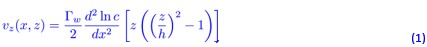
The following is the authors’ response to the original reviews.
Public Reviews:
Reviewer #1 (Public review):
Summary:
The authors identify and investigate a specific population of PVNOT neurons (oxytocin neurons of the paraventricular hypothalamus) that seem to be involved in both behavioral and autonomic thermoregulation. These cells are activated by social thermoregulatory behaviors, but can influence thermoregulation in both social and nonsocial contexts, specifically during transitions and when mice are at low core body temperature (Tb).
Strengths:
The manuscript has many strengths.
This is a novel study, with a clear question that is addressed using an array of well-designed experiments employing integrative methods. Most of the figures are well-developed, and the analysis is generally rigorous and well-detailed. The authors are clearly very experienced in this field, and indeed, their scholarly introduction and discussion sections are to their credit.
We are grateful for the reviewer’s careful reading and positive assessment, including their remarks on the clarity of the question, experimental design, and analysis.
The link between thermoregulation and the oxytocin system is well established, as is the link between social behavior and the same broad system. However, the link between these three things is novel, if it can be well substantiated. I am not persuaded that was achieved here, but I do think this manuscript has many novel and useful offerings.
We thank the reviewer for this thoughtful comment and for recognizing the novelty of the study. We wish to clarify the central goal of the manuscript: while social thermoregulation provided the initial influence for studying PVNOT neurons, our principal finding is that PVNOT activity during rest-to-arousal transitions is independent of social context. As stated in the manuscript, "To our surprise, these peaks were observed in both social and non-social contexts." Thus, our study demonstrates a broader role for PVNOT neurons in state-dependent thermoregulatory transitions—one that includes, but is not limited to, social contexts. We have revised the text to make this emphasis clearer throughout.
We also added a short piece to the Discussion on this point. This is the fourth and final paragraph of the Discussion section called “State-dependent PVNOT activity during thermo-behavioral transitions.”
The authors use a cooling floor, and only go down to 10 degrees Celsius. This is fine, but I would like to see the effects using ambient temperature also. This is not a crucial issue, as it is not necessary for the authors' interpretations, but it could improve measurement sensitivity.
Both Reviewer 1 and Reviewer 2 raise important and related points: manipulating floor temperature provides a thermal stimulus that is distinct from manipulating whole-chamber ambient air temperature, and these modalities could engage partially different sensory pathways and circuits. (Note this response is copy-pasted to other relevant comments).
We intentionally used floor cooling/heating because it provides a reliable, well-controlled stimulus that elicits thermoregulatory behaviors while keeping the experimental environment stable (e.g., avoiding changes in airflow/humidity that can accompany ambient cooling). To prevent conflation of these modalities, we revised the manuscript to consistently describe the manipulation as “floor temperature” (and not “ambient temperature”), and we added to the Discussion acknowledging that conductive floor temperature changes may differentially recruit peripheral thermoreceptors compared to ambient air temperature.
While extending these experiments to whole-chamber ambient temperature changes could be informative in future work, it is not required for the central interpretations here, which focus on PVNOT activity dynamics during thermoregulatory behavior under controlled thermal conditions.
Through an elegant behavioral experiment in Figure 1, the authors identify c-Fos patterns in the PVN that are activated by active social huddling, and they show that at the RNA level these cells overlap with oxytocin, indicating that they are oxytocin-producing cells. But this is not well discussed or indeed quantified.
We thank the reviewer for catching this; Reviewer 2 made a similar comment. A typo in the figure legend led to this confusion. Figure 1I is in fact a quantification of the percent Oxytocin:Fos colocalized cells (not Fos:DAPI, as was written) in dorsal and ventral subregions of the PVN during active huddling and quiescent huddling. We have corrected the legend and clarified the quantification in the revised manuscript.
The authors engage in a deep analysis of fiber photometry experiments, first by observing PVNOT neuron overall activity during a variety of different behaviors in the context of three different temperatures. Activity was associated with nesting, quiescence, and both types of huddling (when social opportunities exist). Social situations did not strongly affect this, nor did temperature conditions. These analyses indicate that the PVNOT neurons are involved in mediating specific behavioral outputs.
With more detailed analysis, the authors investigated how PVNOT neuronal activity relates to behavioral state transition. They found that the probability of peak PVNOT neural activity strongly predicts the offset of quiescence or quiescent huddling, and therefore can be argued to signal an increase in physical activity, and as such, increased metabolism. However, the opposite pattern was observed for huddling and nesting (onset being associated with PVNOT activity), again arguing for increased thermogenesis as a function.
What is particularly compelling is that these peaks of activity tend to occur during low Tb, again arguing for the function in increasing body warmth.
The authors then employ an impressive setup where they image brown adipose tissue (BAT) in tandem with DeepLabCut (DLC) based animal tracking. Crucially, BAT activity and surface temperature correlated with the calcium peak of PVNOT neurons.
Lastly, optogenetic activation of PVNOT neurons increased Tb when it was in the lower range, but not when in the higher range. It also affected BAT and rump temperature, again at low Tb. However, there is no real effect on behavior, except a trend in activity.
The authors do some interesting tracing work at the end, though this is not functionally explored. That is not a criticism, as it does seem like this would be a whole follow-up study.
Weaknesses:
While novel and valuable, the manuscript feels incomplete in its current form.
The main evidence lacking is a loss of function of the experiment. Ideally, the authors would chronically and/or acutely inhibit PVNOT neurons to establish their necessity. I know this seems obvious, but I think it is important.
We agree with the reviewer that loss-of-function experiments are a valuable component of circuit mapping and we appreciate this suggestion. For transparency, we did attempt a chronic chemogenetic inhibition experiment using DREADDs in PVNOT neurons. However, the results were inconclusive, primarily owing to the confounding effects of pharmacological injections: both drug and vehicle-treated animals exhibited stress-induced hyperthermia following injection, and because inhibition could not be delivered while animals were asleep/resting the experimental conditions did not recapitulate the low-Tb quiescent state during which PVNOT peaks naturally occur. Given these confounds, we do not believe these data meet the standard required for inclusion in this manuscript.
We did consider acute optogenetic inhibition. However, a clear prediction about inhibition was not as apparent in our model. Our photometry data identified a, testable hypothesis for activation: PVNOT peaks precede the exit from quiescence, therefore activation during quiescence should increase the transition, which it did (Figures 5 and 6).
That said, new analyses of our data, driven by these reviews, have now uncovered what might be inhibition of PVNOT neurons during the approximate 60 seconds prior to entry to resting states (i.e., quiescence and quiescent huddling); see the new Fig. S3I-L. This raises the possibility that an appropriately timed photoinhibition of PVNOT neurons could facilitate the establishment of resting states. We believe that, in light of our chemogenetic and optogenetic activation experiments, for an inhibition experiment to be done appropriately would require a real-time, closed loop setup that is currently not available in our laboratory.
We have added a caveat to the Discussion acknowledging the lack of LOF data as a limitation and have identified this as an important direction for future investigation.
The relative lack of behavioral analysis following optogenetic activation of PVNOT neurons is puzzling. The authors must surely want to study what this intervention does to behavioral state transitions. I feel that the current level of analysis limits the overall conclusions of this study to a large extent.
We appreciate this concern and wish to clarify two points.
First, our decision to perform optogenetic activation in isolated (solo-housed) animals was driven by our initial finding that PVNOT activity profiles are mostly social-context independent during the transition from rest to arousal (Figures 2 and 3). By studying isolated animals, we could test the fundamental relationship between PVNOT activation and the rest-to-active transition without confounding social feedback. Additionally, we encountered technical challenges when using the SGBS thermographic model in paired contexts: the high thermal intensity at the point of contact between huddling mice created a thermal merging artifact that prevented accurate segmentation of individual body regions (BAT vs. rump).
Second, we did examine the post-stimulation behaviors of solo-housed animals (Fig. S5B). While PVNOT activation significantly increased the probability of exiting quiescence, it did not trigger a singular, stereotyped behavioral output. Instead, it facilitated a generalized transition to an active state, within which animals engaged in various context-appropriate actions (nesting, grooming, locomotion). We note in the discussion that “Analysis of manually- annotated behaviors suggested that PVNOT stimulation did not activate a specific motor pattern output but instead resulted in combined increases in the time spent in nesting (linear mixed model estimate coefficient of ChR2+ stimulation: +38.0 sec), locomotion (+54.0 sec), and grooming (+14.5 sec), but not in eating/drinking (-0.4 sec) (Fig. S4B).”
That photostimulation had relatively larger effects on nesting and locomotion is consistent with our model.
Last, in the Discussion we acknowledge that future experiments should seek to disentangle the effects of PVNOT light simulation in the non-social vs social context (last paragraph of the Discussion section called “State-dependent PVNOT activity during thermo-behavioral transitions”).
A broader criticism is that the social dimension of this manuscript seems overplayed. Naturally, oxytocin signaling can be implicated in social behavior based on a large literature. However, the focus on social thermogenesis seems like a crude integration of social behavior and thermogenesis. Given that the authors see their effects in both social and nonsocial cases of thermoregulation, I am not sure the attempts at integrating social functions and thermogenic functions of PVNOT neurons are warranted. That is, unless the authors have further experiments or analysis that can convincingly justify this link.
We thank the reviewer for this comment. We understand the concern and wish to reframe our position. We argue that the equivalence of PVNOT signals across social and non-social contexts is itself a central finding. While the oxytocin system is widely regarded as a mediator of social bonding, and therefore a candidate mechanism underlying huddling, our data demonstrate that PVNOT neurons provide a signal for state-dependent thermoregulatory transitions that is unbiased by social context. Rather than overplaying the social dimension, we believe our study contextualizes the social function within a broader homeostatic role: PVNOT neurons facilitate transitions from rest to thermogenesis and arousal regardless of whether the resting state involves social huddling or solitary quiescence.
While the thermoregulatory transitions are present in both contexts, we note that social context appears to modestly enhance some PVNOT downstream effects. Specifically, peak probability and frequency were slightly higher in the paired compared to solo context (Fig. 3F-I, Fig. S2D), and peaks were associated with a somewhat stronger increase in physical activity when a cagemate was present (Fig. 3B-E). Additionally, quiescent huddling (paired) bouts were associated with stronger body temperature regulation compared to solo quiescence (Fig. S3Q-V). This nuance supports that the social dimension is not overplayed but rather situated within a broader homeostatic function.
We have revised the manuscript to ensure that this framing is consistent and clear. We emphasize that our goal was to uncover neural mechanisms underlying physiological transitions across behavioral and arousal states, using our social thermoregulation assay as a starting point (based on our previous publication). Counter to our initial hypothesis, the PVNOT signals generalized beyond the social setting.
In addition, the analysis of virgin females and lactating mothers seems out of place in Figure 4.
This point was echoed by Reviewers 1 and 3, and one we have taken several actions to address this. (Note this response is copy-pasted to the other reviewers).
We agree with the reviewers that the rationale for the lactation data should be made more explicit. The primary purpose of this experiment was to validate the identity of oxytocinergic neurons of the PVN.
Our efforts to use IHC to validate the identity of AAV-transfected cells were inconclusive, and we have now added new data to illustrate this point. We have added Fig. S4 that includes quantitative data on expression specificity. We observed significant variability in co-staining (OT+/GCaMP+) across brain slices, likely reflecting the dynamic nature of oxytocin peptide synthesis and storage, particularly with respect to processes lining the third ventricle. This finding is in accordance with other studies that are now cited in the text.
We now emphasize that, because IHC provided variable co-localization, we employed the lactation model as an independent physiological validation of the identity of the recorded neurons.
It is well established that PVNOT neurons undergo dramatic changes in firing dynamics and synchrony during lactation to support milk ejection (Yaguchi et al., 2023; Yukinaga et al., 2022). Conversely, AVP and CRF cell populations in the PVN do not appear to display synchronized pulsatile bursting during lactation (see response to Reviewer-2 comment-2 in ‘Recommendation for authors’ and our updated Discussion). Observing these characteristic changes in our recorded population provides high-confidence functional evidence that we are targeting oxytocin neurons. We have revised the text to clarify that Figure 4 serves primarily as a functional verification of genetic targeting.
We also acknowledge in the Discussion the possibility that our Cre-line may capture a small percentage of nonoxytocinergic neurons, while noting that the dramatic shift in calcium dynamics during lactation (Figure 4I–L) strongly suggests the recorded population is dominated by oxytocin neurons.
The c-Fos/oxytocin overlap needs to be quantified.
We thank the reviewer for catching this; Reviewer 2 made a similar comment. A typo in the figure legend led to this confusion. Figure 1I is in fact a quantification of the percent Oxytocin:Fos colocalized cells (not Fos:DAPI, as was written) in dorsal and ventral subregions of the PVN during active huddling and quiescent huddling. We have corrected the legend and clarified the quantification in the revised manuscript. (Note this response is copy-pasted to other relevant comments).
The methods section could be improved by explaining how the authors exclude animals that exhibit both types of huddling, if they occur within a 90-minute time window. This seems like it could cause significant confounds.
We have clarified in the Methods that animals were not excluded if they exhibited both active and quiescent huddling during the recording session. Importantly, a prerequisite for inclusion in the FOS study was that animals had to be continually engaged in the target behavior for a minimum of 15 consecutive minutes from behavior onset, an established approach for behavior-driven immediate early gene mapping. The 90-minute window was then counted from that same onset for FOS IHC. Because active huddling frequently transitions directly into quiescent huddling (and vice versa), excluding such animals would have eliminated the majority of recordings. The heterogeneity of behavioral states within the FOS integration windows is precisely why we turned to fiber photometry, a technique with the temporal resolution necessary to dissociate neural signals associated with each behavioral state.
The computer vision model is not well-explained. The authors need to be far more explicit here about how it was validated.
We thank the reviewer for this comment and agree that the original manuscript did not sufficiently detail the validation framework. We have revised both the Methods and Results to explicitly detail how SGBS was evaluated.
First, we now clearly describe model validation on a held-out dataset (20% of manually annotated images not used for training), reporting standard segmentation metrics (per-class IoU and Dice/F1) and directly comparing SGBS to an unmodified Mask R-CNN trained under identical conditions (same backbone initialization, dataset split, and training schedule). As shown in Fig. 5D, the skeleton-guided model converged more rapidly and achieved a lower final loss than the baseline network, demonstrating improved segmentation performance in occlusion-rich thermographic recordings.
Second, we more explicitly describe an independent physiological validation step. SGBS-derived surface temperature trajectories were temporally aligned with simultaneously recorded implanted thermologger measurements, which were not used during model training. As shown in Fig. 5E, SGBS-derived signals strongly corresponded with core body temperature dynamics and reproduced expected thermophysiological relationships (e.g., BAT warming preceding core temperature rise). This establishes external validity beyond pixel-level segmentation metrics.
The authors should cite and consider this preprint: https://www.biorxiv.org/content/10.1101/2024.09.17.613378v1
We have cited this preprint (Raam et al., 2024) in the revised manuscript and integrated relevant findings into the Discussion, in the section called “Limitations and caveats”.
Reviewer #2 (Public review):
Summary:
This is a very interesting study from Vandendoren and colleagues examining the role of PVN oxytocin neurons during thermoregulatory behaviors, in particular during thermoregulatory huddling. The findings are important and compelling, and have implications for the thermoregulation field as well as the social/naturalistic behavior field.
Strengths:
The study is very creative and tackles a challenging task to examine how natural and social behavior influences neural circuits for a homeostatic system such as thermoregulation. The authors use a combination of state-of-the-art tools (photometry, optogenetics, automated behavior tracking, thermal imaging, and core body temperature measurement), often in combination with each other, to produce a rigorous and high-dimensional dataset. Carrying out tightly temperature-controlled experiments and examining natural behavior, neural activity, and body physiology simultaneously is quite a feat. I applaud the authors for taking this on in a rigorous and detailed manner. This paper will be valuable for both the thermoregulation field as well as for researchers interested in naturalistic social behaviors. The conclusions are supported by the data.
We appreciate the reviewer’s careful read and positive assessment of our integrated behavioral, neural, and physiological measurements and their relevance to both thermoregulation and social behavior.
Weaknesses:
I have a number of questions and suggestions for clarification that would help improve the interpretation of the findings.
(1) Figure 1D-F: It would be helpful to include representative images of cFos expression in the PVN, LS, and DMH during both quiescent and solo huddling conditions, to better illustrate the reported differences.
We have now addressed this in the revised manuscript. We had originally shown active huddle FOS expression in Fig. 1D-F and quiescent huddle in Fig. S1A-C. We have now added solo groom FOS expression to Fig. S1D-F.
(2) Figure 1C: The data suggest a general suppression of neural activity during sleep-associated quiescent huddling, which somewhat complicates the interpretation of what specifically the active huddling cells are responding to. A more informative control might have been a comparison between huddling and a more generic form of social engagement (e.g., dyadic sniffing) to assess whether huddling-responsive neurons are broadly tuned to social stimuli. While it may not be feasible to add this experimentally at this time, a brief discussion of this limitation in the main text would be valuable.
We thank the reviewer for this thoughtful suggestion. We agree that comparing huddling-responsive neurons with a more generic social engagement is an important consideration.
We first note that the FOS study required animals to be continuously engaged in the target behavior for a minimum of 15 consecutive minutes, ensuring that FOS expression reflects sustained behavioral engagement rather than brief social contact. Furthermore, we believe the FOS association with active huddling in Figure 1C is likely driven by preceding bouts of quiescent huddling. Because these experiments were conducted during the light phase, active huddling bouts were almost always preceded by bouts of quiescent huddling.
Given that FOS protein often integrates neural activity over ~60-90 minutes, the FOS signal during active huddling may reflect cumulative PVNOT activity during the quiescent to active transition, rather than active huddling by itself. This interpretation aligns with our fiber photometry data, which show that PVNOT peaks are concentrated at the offset of quiescent states and the onset of active states. Moreover, a broad-scale analysis of calcium data driven by these reviews, now shows there is a local minimum of PVNOT neurons during the transition into quiescent states and a local maximum of calcium activity during the offset of resting states and the onset of nesting and active huddling (Fig. S3I-L).
To directly address whether PVNOT neurons are broadly tuned to social engagement or specifically associated with thermoregulatory state transitions, we examined neural activity during "Contact Initiated" (ConI) and "Contact Received" (ConR) events—brief social interactions (e.g., dyadic sniffing) that occur outside the context of huddling. These interactions, which typically last less than one second, did not trigger the large-amplitude calcium peaks observed during rest-to-arousal transitions. Specifically, there was no significant association between ConI or ConR events and PVNOT peak frequency or amplitude (Fig. S2H; Table S1; p = 0.505, p = 0.575, respectively). This reinforces our conclusion that PVNOT peaks are not a generic response to social stimuli but are specifically aligned with the coordinated autonomic and behavioral transitions required to exit a low-temperature quiescent state. We have added a clarifying paragraph to the Discussion.
(3) Figure 2H-J vs. Figure 1: The fiber photometry data suggest increased PVN activity during quiescent huddling vs active huddling, which appears to contrast with the cFos results from Figure 1. It would be helpful for the authors to comment on possible reasons for this discrepancy-e.g., methodological differences, temporal resolution, or cell-type specificity.
We agree that this apparent contrast deserves explicit discussion. The difference arises from the dramatically different temporal resolutions of the two techniques. Fiber photometry captures real-time neural dynamics at subsecond resolution, revealing that PVNOT neurons exhibit high-amplitude bursts primarily during the offset of quiescence (and to a lesser extent the onset of post-quiescence behaviors) (Figs. 3 and 5). Because these peaks occur while the animal is categorized as "quiescent," they appear as quiescence-associated activity in the photometry ethogram.
Conversely, FOS integrates neural activity over ~30–90 minutes. In retrospect, and in light of our photometry data, an animal categorized as "Active Huddling" in the FOS study is one that has likely experienced PVNOT bursts and subsequently transitioned to an active state. The higher FOS signal in active animals therefore likely represents the cumulative activity of the transition itself and sustained activity in the active state.
We have added a clarifying statement to the Discussion section, in the section called “State-dependent PVNOT activity during thermo-behavioral transitions”.
(4) Figure 2O: A comparable linear regression for active huddling would be informative to assess whether the observed relationships extend across behavioral states.
We agree. We have added linear regression analyses for active huddling and nesting to Fig. S2K-N including rsquared values, to complement the resting analyses in Figure 2O and 2L.
This analysis shows that active huddling peak counts are also positively correlated with active huddle duration (but not nesting duration). The text has been updated accordingly.
(5) Temperature manipulation: The use of floor temperature changes presents a distinct physiological and sensory experience from, for example, manipulation of ambient temperature. A discussion of how this choice may affect neural circuit engagement or interpretation of thermoregulatory responses would be beneficial.
Both Reviewer 1 and Reviewer 2 raise important and related points: manipulating floor temperature provides a thermal stimulus that is distinct from manipulating whole-chamber ambient air temperature, and these modalities could engage partially different sensory pathways and circuits. (Note this response is copy-pasted to other relevant comments).
We intentionally used floor cooling/heating because it provides a reliable, well-controlled stimulus that elicits thermoregulatory behaviors while keeping the experimental environment stable (e.g., avoiding changes in airflow/humidity that can accompany ambient cooling). To prevent conflation of these modalities, we revised the manuscript to consistently describe the manipulation as “floor temperature” (and not “ambient temperature”), and we added Discussion acknowledging that conductive floor temperature changes may differentially recruit peripheral thermoreceptors compared to ambient air temperature.
While extending these experiments to whole-chamber ambient temperature changes could be informative in future work, it is not required for the central interpretations here, which focus on PVNOT activity dynamics during thermoregulatory behavior under controlled thermal conditions.
(6) Correlations with behavior: Across the manuscript, it would be informative to see correlations between huddle duration and neural activity (e.g., cFos expression, calcium signal magnitude). Similarly, do longer huddles produce greater thermogenic effects?
This is a great suggestion. The first point about huddle duration and neural activity echoes the Reviewer’s comment (4) above. For this point, we now show that the duration of active huddling is positively correlated with PVNOT peak count (Fig. S2K), which is similar to what we had shown for quiescence and quiescent huddling (Fig. 2K-P).
Next, the point about huddle duration and thermogenic effects is also helpful. We have now added new analysis and panels to address this (Fig. S3M-R). We find that the duration of quiescent huddle bouts is negatively correlated with Tb (Fig. S3V). The other behaviors examined did not show correlations between duration and Tb. This finding supports our previous demonstration that quiescent huddling is an energy saving state in mice (Landen et al., 2024).
Finally, we note that longitudinal correlations between bout length and peak counts are already reported in Fig. S3A-H.
(7) Lactating vs. virgin mothers: The inclusion of maternal data is intriguing but feels somewhat disconnected from the central huddling-thermoregulation narrative. If these experiments are to remain, additional explanation of their rationale and how they fit into the broader story would help clarify their relevance.
This point was echoed by Reviewers 1 and 3, and one we have taken several actions to address this.
We agree with the reviewers that the rationale for the lactation data should be made more explicit. The primary purpose of this experiment was to validate the identity of oxytocinergic neurons of the PVN.
Our efforts to use IHC to validate the identity of AAV-transfected cells were inconclusive, and we have now added new data to illustrate this point. We have added Fig. S4 that includes quantitative data on expression specificity. We observed significant variability in co-staining (OT+/GCaMP+) across brain slices, likely reflecting the dynamic nature of oxytocin peptide synthesis and storage, particularly with respect to processes lining the third ventricle. This finding is in accordance with other studies that are now cited in the text.
We now emphasize that, because IHC provided variable co-localization, we employed the lactation model as an independent physiological validation of the identity of the recorded neurons.
It is well established that PVNOT neurons undergo dramatic changes in firing dynamics and synchrony during lactation to support milk ejection (Yaguchi et al., 2023; Yukinaga et al., 2022). Conversely, AVP and CRF cell populations in the PVN do not appear to display synchronized pulsatile bursting during lactation (see response to Reviewer-2 comment-2 in ‘Recommendation for authors’ and our updated Discussion). Observing these characteristic changes in our recorded population provides high-confidence functional evidence that we are targeting oxytocin neurons. We have revised the text to clarify that Figure 4 serves primarily as a functional verification of genetic targeting.
We also acknowledge in the Discussion the possibility that our Cre-line may capture a small percentage of non-oxytocinergic neurons, while noting that the dramatic shift in calcium dynamics during lactation (Figure 4I–L) strongly suggests the recorded population is dominated by oxytocin neurons.
(8) Optogenetic manipulation: Have the authors tested the effect of PVN OT neuron stimulation or inhibition during huddling? Even a negative result would be of interest to the field. If these data exist (main or supplementary), I apologize for missing them. If not, the authors might consider including them or commenting briefly on any attempts or challenges in carrying out these experiments.
We thank the reviewer for this question. We have not performed optogenetic manipulation during huddling. Our decision to perform optogenetic activation in solo-housed animals was driven by our fiber photometry finding that PVNOT activity profiles during the rest-to-arousal transition are social-context independent (Figures 2 and 3). Had the GCaMP data suggested that PVNOT peaks were specific to social huddling, optogenetic manipulation during huddling would have been the natural next experiment. However, because peaks aligned with thermoregulation broadly, rather than social behavior specifically, we designed our functional experiments to test the circuit's role in driving the autonomic and behavioral arousal transition.
We also note that our experience with chemogenetic manipulation suggests that pharmacological approaches to study the rest-arousal transitions during huddling are not currently feasible. As described to our response to Reviewer 1, our DREADD inhibition experiments were confounded by stress-induced hyperthermia following injection, and because drug delivery could not occur while animals were asleep and resting, the experimental conditions failed to recapitulate the low-Tb quiescent state during which PVNOT peaks naturally occur. We share this experience because we believe it will be informative for others in the field considering similar approaches.
Additionally, as described above (Reviewer 1, #5), the SGBS thermographic model encounters artifacts in paired contexts due to thermal merging between huddling mice. We have added a note in the Discussion addressing this, in the section called “Limitations and caveats”.
Reviewer #3 (Public review):
Summary:
The authors aimed to elucidate the relationship between physiological state (i.e., behavioral status and thermogenic sympathetic activity) and the activity of hypothalamic paraventricular oxytocin (PVNOT) neurons in female mice. They studied this by combining automated classification of mouse behavior via video-based analysis with calcium imaging of PVNOT neuron activity. Sympathetic thermogenesis was inferred from surface temperature changes captured by infrared thermography, and the authors provided their custom analysis scripts in the manuscript. Notably, they found that a strong, pulsatile activation of PVNOT neurons was "occasionally" observed immediately before the animals transitioned from a resting to an active state. This pulsatile activity was observed in both pair-housed and individually housed animals. While PVNOT neurons are often associated with social behaviors, this finding suggests that the oxytocinergic system is also engaged during naturalistic behaviors, even in the absence of social interactions. If experiments were more convincingly performed and presented, the results would point to a broader physiological role of central oxytocin, including in the regulation of fundamental brain states and homeostatic processes, and offer a new perspective on the functional significance of central oxytocin signaling.
Strengths:
The oxytocinergic neural system is believed to subserve a wide range of physiological functions, and elucidating these roles requires monitoring PVNOT neuronal activity under various behavioral contexts, as well as manipulating this activity to establish causal links. In the present study, the authors show a technically sound experimental framework that integrates behavioral tracking in both individually and group-housed mice with the observation and manipulation of PVNOT neuron activity. This experimental setup represents a valuable methodological resource for researchers investigating the physiological functions of oxytocin.
We thank the reviewer for the thoughtful review and for recognizing the value of our integrated framework for monitoring and manipulating PVNOT neuronal activity across behavioral contexts.
Weaknesses:
While this study successfully established a new experimental setup for simultaneous analyses of behavior and PVNOT neuronal activity, there are several concerns regarding the interpretation of the results and the robustness of the conclusions, which should be more thoroughly addressed.
(1) The study relies on the assumption that calcium imaging and optogenetic manipulation were restricted only to PVNOT neurons. However, the specificity of AAV-mediated gene expression was not verified quantitatively. A fair number of cell bodies in the PVN expressed GCaMP8s, but not OT, indicating potential off-target expression (see Figure S2A, B). The lack of quantitative validation weakens confidence in the causal interpretation of the results.
This point was echoed by Reviewers 1 and 3, and one we have taken several actions to address this.
We agree with the reviewers that the rationale for the lactation data should be made more explicit. The primary purpose of this experiment was to validate the identity of oxytocinergic neurons of the PVN.
Our efforts to use IHC to validate the identity of AAV-transfected cells were inconclusive, and we have now added new data to illustrate this point. We have added Fig. S4 that includes quantitative data on expression specificity. We observed significant variability in co-staining (OT+/GCaMP+) across brain slices, likely reflecting the dynamic nature of oxytocin peptide synthesis and storage, particularly with respect to processes lining the third ventricle. This finding is in accordance with other studies that are now cited in the text.
We now emphasize that, because IHC provided variable co-localization, we employed the lactation model as an independent physiological validation of the identity of the recorded neurons.
It is well established that PVNOT neurons undergo dramatic changes in firing dynamics and synchrony during lactation to support milk ejection (Yaguchi et al., 2023; Yukinaga et al., 2022). Conversely, AVP and CRF cell populations in the PVN do not appear to display synchronized pulsatile bursting during lactation (see response to Reviewer-2 comment-2 in ‘Recommendation for authors’ and our updated Discussion). Observing these characteristic changes in our recorded population provides high-confidence functional evidence that we are targeting oxytocin neurons. We have revised the text to clarify that Figure 4 serves primarily as a functional verification of genetic targeting.
We also acknowledge in the Discussion the possibility that our Cre-line may capture a small percentage of nonoxytocinergic neurons, while noting that the dramatic shift in calcium dynamics during lactation (Figure 4I–L) strongly suggests the recorded population is dominated by oxytocin neurons.
(Note, we have updated Figure S2A,B to more accurately reflect the extent of co-localization in this image).
(2) The study focuses on the transition from rest to active states following pulsatile activity of PVNOT neurons. However, the physiological significance of this pulsatile activity remains unclear. According to the authors, pulsatile activity occurred with an approximately 20% probability within 100 seconds prior to the end of the resting state. This implies that, in the remaining 80% of rest-to-active transitions, pulsatile PVNOT activity did not occur, suggesting that it is not essential for initiating the transition. A comparative analysis of behavioral and thermogenic changes between transitions with and without pulsatile PVNOT activity would help to further clarify the functional relevance of this phenomenon and strengthen the authors' interpretation of the findings.
These are excellent points, and here we address them separately.
(1) probability of transitions.
We agree that our wording could be misread and we have revised the text for clarity. The “~20%” value is not the fraction of rest-to-active transitions that exhibit pulsatile PVNOT activity within a 100-s window. Instead, Fig. 3F,H report an instantaneous (per-second) probability of observing a calcium peak as a function of time-to-bout offset (logistic regression). In other words, the probability of a peak increases sharply as the animal approaches rest offset (e.g., from ~2–3%/s near onset to ~14%/s for quiescence and ~25%/s for quiescent huddling near offset), indicating a strong state-dependent increase in peak likelihood rather than an all-or-none trigger.
We further clarify in the Discussion that we do not claim PVNOT peaks are essential for initiating every transition; rather, PVNOT activity biases or enhances the probability of transition toward thermogenesis and behavioral arousal (added to section called “State-dependent PVNOT activity during thermo-behavioral transitions”).
(2) the effect of peaks on transitions
This is a very helpful suggestion and we agree that directly comparing transitions with vs. without pre-offset pulsatile PVNOT activity could strengthen interpretation of the functional relevance of these events. We have therefore added a new transition-aligned analysis of thermogenic dynamics at rest-to-active transitions (new Fig. 3P&S; and corresponding text in the Results and Statistics sections).
Briefly, we extracted peri-transition body temperature (Tb) traces (−300 to +300 s) aligned to the offset of quiescence and quiescent-huddling bouts and classified each transition as Peak+ if it contained one or more calcium peaks in the 100 s preceding bout offset, and Peak− otherwise. To account for inter-individual differences in “balance point,” Tb was z-scored within mouse. We then quantified the post-offset thermogenic rise for each transition as the change in scaled temperature from a pre-offset baseline (−60 to 0 s) to the post-offset interval (0 to 300 s) and tested Peak+ vs Peak− differences using linear mixed-effects models. This revealed that Peak+ transitions exhibited significantly larger post-offset increases in scaled Tb than Peak− transitions for both quiescence offsets and quiescent-huddling offsets.
Together, these results indicate that while pulsatile PVNOT activity is not present prior to every rest-to-active transition, when it occurs it is associated with a stronger thermogenic rise, consistent with a probabilistic modulatory role in promoting the transition rather than being strictly required to initiate it.
We are grateful for this suggestion as this new data is very informative in the context of our model.
(3) The study identifies a correlation between pulsatile activity of PVNOT neurons and rest-to-active transitions, and tests for a causal relationship using optogenetic stimulation. However, since PVNOT neurons are known to co-release other neurotransmitters such as glutamate, it remains unclear whether the observed effects are mediated specifically through oxytocin receptor signaling. To address this question, functional intervention experiments using oxytocin receptor antagonists or receptor knockout mice are necessary.
We agree with the reviewer that PVNOT neurons co-release glutamate and that isolating the specific contribution of oxytocin signaling versus co-transmitted signals is an important question. However, our study was designed to identify the functional role of the PVNOT cell type during thermoregulatory state transitions, not to dissect the molecular mechanism of signaling at downstream targets. By demonstrating that the endogenous activity of this specific population aligns with the rest-arousal window and that their activation is sufficient to drive the phenotype, we provide an anatomical and functional framework for future mechanistic investigations.
We also note that we provide anatomical evidence supporting a possible peptidergic mechanism: PVNOT neuron projections to the rostral medullary raphe (rMR), a key thermogenic control site, alongside oxytocin receptor mRNA expression in this region (Fig. S5). This anatomical link suggests a plausible pathway for oxytocinergic modulation of thermogenesis, but of course does not rule in/out glutamatergic signaling. We acknowledge this limitation in the Discussion and frame pharmacological and receptor knockout studies as important next steps.
We address these points in the Discussion, in the section called “Limitations and caveats.”
(4) The authors attempted to detect BAT thermogenesis and skin vasomotion using infrared thermography. This technique measures only skin hair temperatures (since the skin was not shaved), but does not measure "BAT temperature" or "vasomotor tone". As seen in Figure 5E, the temperatures of the body surface areas ("BAT", "Rump", and "Dorsal surface") mostly changed in parallel, indicating that these temperatures are strongly affected by body core temperature. Therefore, the thermographic measurements in this study did not provide convincing information on BAT thermogenesis or skin vasomotion. To avoid misleading reports, the authors need to use other techniques to directly measure temperatures, such as telemetry.
We agree that infrared thermography measures surface radiance rather than internal tissue temperature. We have revised the manuscript to use more precise language (e.g., "surface temperature over the interscapular BAT region" rather than "BAT temperature"). However, surface measurements are not merely passive reflections of core temperature. Here we add background and explanation about our thermography data:
Background on our approach
Infrared thermography provides a non-invasive readout of heat emission over the interscapular region and has been validated as reporting UCP1-dependent BAT thermogenesis in mice under adrenergic stimulation (Crane et al., 2014). That said, there are known confounds (insulation/adiposity, blood flow, protocol variability) and standardized protocols are needed (Law et al., 2018). Direct telemetry or implanted thermocouples offer superior precision for measuring BAT temperature, so long as the probe is sutured to BAT itself or to Sulzer’s vein–a technical challenge because probes tend to drift over time (e.g., (Dodson et al., 2024)).
Our BAT findings in context:
Using SGBS, we demonstrate that the interscapular BAT region is significantly warmer than the adjacent rump surface (Fig. 5C). If surface temperature were purely a reflection of uniform core temperature, this consistent regional hotspot would not be observed.
Our cross-correlation analysis from the photometry (Fig. 5E) shows the rise in BAT surface temperature precedes changes in other body regions by approximately 90 seconds, suggesting that BAT acts as a primary heat source during rest-to-arousal transitions rather than passively following core temperature. This finding is consistent with another study, using telemetric probes placed in BAT, finding that episodic onset of BAT temperature started to increase 3 minutes before body temperature (Ootsuka et al., 2009).
Based on this Reviewer’s comment here and the subsequent one (5), we have now added a new analysis of the temporal patterning of arousal and thermogenesis in the optogenetic cohort of animals; see below for details.
Vasomotor tone
We agree that infrared thermography does not directly measure vasomotor tone. We have revised the text to remove language implying that our measurements directly quantify vasomotor tone, vasodilation or vasoconstriction.
We note that the established approach for non-invasive assessment of vasomotion uses glabrous skin of the tail and ears (Garami et al., 2011; Meyer et al., 2017; Škop et al., 2020). Rump surface temperature measured over hairy, non-glabrous skin correlates more closely with core body temperature than with cutaneous vasomotor tone (Meyer et al., 2017; Škop et al., 2020) and is used in the literature as a reference point for calculating BAT thermogenesis.
In our data, rump surface temperature decreased following PVNOT calcium peaks while BAT and dorsal surface temperatures increased (Fig. 5L-M). This pattern is consistent with sympathetically-driven thermogenesis in which peripheral heat loss is reduced while BAT drives core temperature upwards. We now acknowledge that our rump measurements do not isolate vasomotor contributions. We have revised the manuscript accordingly, replacing references to rump vasoconstriction with language describing the observed thermal pattern while avoiding attribution to a specific thermoeffector mechanism.
Finally, we note that telemetry would strengthen deep-body temperature interpretation, but telemetry does not itself quantify vasomotor tone; the same distal heat-loss readouts described above would be required regardless of core Tb methodology.
In sum, infrared thermography enables non-invasive, simultaneous tracking of multiple thermal features in freely moving, undisturbed animals—a requirement for studying the naturalistic state transitions central to this study. We have added a section to the Discussion acknowledging the limitations of surface infrared thermography.
(5) Photostimulation of PVNOT neurons increased Tb after 400 sec (6.6 min) (Figure 5). This latency is too long to conclude that the neuronal stimulation elicited BAT thermogenesis. A more reasonable explanation is that the increase in Tb was caused by the induction of physical activity (Figure S4C), which slowly generates heat and contributes to the elevation of Tb. However, this view contradicts the authors' claim. To address this concern, the authors should directly measure BAT thermogenesis and compare it with the rate of Tb elevation. If BAT thermogenesis occurs, the rate at which the BAT temperature increases must exceed the rate at which Tb rises.
We thank the reviewer for this thoughtful critique. With this response we first provide additional context about the timeline of temperature increases, and second add a new analysis addressing the relative contributions of activity and BAT-surface to Tb changes.
(1) Additional context on the temporal progression
First, the observed timescale does not, per se, rule out a contribution of BAT thermogenesis. While the kinetics of BAT activation and associated Tb increases can operate on a fast timescale in anesthetized animals, in vivo activation of BAT thermogenesis pathways can take several minutes to yield a statistically detectable difference. For example, activation of DMH→rMR glutamatergic signaling, a canonical thermogenic command pathway, takes several minutes to produce a significant increase in both Tb and BAT using telemetric temperature probes (Kataoka et al., 2014).
This timescale could also be consistent with peptidergic neuromodulation by PVNOT neurons, which are more likely to be modulators (and not drivers) of the canonical thermogenic pathway. Oxytocin is known to act via volume transmission and metabotropic receptor signaling, which operate on slower timescales than ionotropic neurotransmission (Ludwig and Leng, 2006). Downstream recruitment of sympathetic outflow and BAT thermogenesis is likewise a multistep autonomic process, not an immediate synaptic event.
Next, the thermal dynamics reported in Figure 5 and Figure S4 are not consistent with activity-induced heat production alone. Specifically:
- Thermal increases were spatially localized to interscapular/dorsal regions corresponding to BAT depots before generalized surface warming.
- Importantly, photostimulation-induced warming was observed even during behavioral states characterized by low baseline activity, suggesting that thermogenic activation was not simply a byproduct of movement.
While we did not directly measure BAT sympathetic nerve activity, our surface thermography approach was designed specifically to resolve regional temperature dynamics over the interscapular BAT area. The spatial specificity and temporal profile of the warming are consistent with BAT thermogenesis rather than uniform musclegenerated heat.
We acknowledge that direct measurement of BAT sympathetic activity or oxygen consumption would provide additional mechanistic resolution. However, given (i) the known role of PVN oxytocin neurons in autonomic regulation, (ii) the spatially localized dorsal temperature increase, and (iii) the temporal dissociation between stimulation onset and gradual systemic Tb rise, we conclude that BAT thermogenesis remains the most parsimonious explanation.
We have revised the Discussion to more explicitly acknowledge these temporal dynamics by clarifying that photostimulation likely follows the timescales of peptidergic neuromodulation.
(2) New analysis
We have added a new analysis to address the relationship between Tb and BAT-surface temperature and locomotion the optogenetic cohort. In short, we show that across all mice changes in BAT typically precede changes in Tb, and that the effect of optogenetic stimulation on core Tb can’t be explained by physical activity (nor can it be explained by BAT-surface temperature).
First, cross-correlation of derivatives suggested BAT surface temperature changes typically precede changes in dTb/dt across mice, whereas physical activity changes did not consistently precede dTb/dt. This result, now shown in Fig. S5G, is consistent with our cross-correlation analysis of the fiber-photometry cohort.
Next, we used a lagged regression analysis to test whether photostimulation-evoked increases in core temperature are fully mediated by physical activity. Specifically, we modeled the derivative of core Tb (dTb/dt) using an impulseresponse representation of photostimulation, while controlling for distributed lags (0–120 s) of physical activity and BAT surface temperature derivative, with random effects for mouse and trial. Photostimulation remained a significant predictor of dTb/dt while controlling for activity and BAT-surface (likelihood ratio test, χ<sup>2</sup>=7.66, p=0.0056), indicating that the relationship between stimulation and Tb is not fully explained by activity.
Recommendations for the authors:
Editors note:
We suggest including key statistical support for the claims in the main text (e.g., results or figure legends).
We have added statistical support for key claims in the main text results. We have also added references to Table S1 where appropriate (e.g., where there is a long list of statistical results); we hope this aids the readability of the report.
Reviewer #1 (Recommendations for the authors):
See above - the authors should decide what to prioritize, but I only mention significant concerns above. The manuscript could be improved to 'Convincing' or even 'Compelling' with sufficient effort.
Thanks for the careful reading of the manuscript. We’ve addressed many of these points, and feel the manuscript has been strengthened as a result.
There were also some text errors here and there.
Several text errors were identified and fixed. Thank you.
Reviewer #2 (Recommendations for the authors):
(1) Figure 1I: The quantification shown here is a bit unclear from the figure and legend - are the authors reporting the percentage of cFos+ cells within the OXT+ population, or within the general DAPI+ population? If the latter, including a co-localization analysis to estimate the proportion of OXT+ cells activated would strengthen the interpretation.
We thank the reviewer for catching this; Reviewer 1 made a similar comment. A typo in the figure legend led to this confusion. Figure 1I is in fact a quantification of the percent Oxytocin:Fos colocalized cells (not Fos:DAPI, as was written) in dorsal and ventral subregions of the PVN during active huddling and quiescent huddling. We have corrected the legend and clarified the quantification in the revised manuscript. (Note this response is copy-pasted to other relevant comments).
(2) PVN cell types: It would be useful to briefly discuss the potential involvement of other PVN populations (e.g., CRF, AVP neurons) in huddling, given their known roles in social behavior, stress, and thermoregulation.
Thank you for the insightful comment. We address these points in two parts.
(1) PVN cell types and huddling
Regarding the specific connection between these cell types and huddling: to our knowledge, no study has directly tested the effect of PVN CRF or PVN AVP neuron manipulation on huddling behavior. The most relevant data come from Bendesky et al. (Bendesky et al., 2017), who found that intracerebroventricular administration of AVP in Peromyscus inhibited nest building but had no effect on huddling, licking, or pup retrieval (though this pharmacological approach does not isolate PVN AVP neurons specifically). Their chemogenetic manipulation of PVN AVP neurons in Mus musculus confirmed the nest-building effect but did not assess huddling. For CRF, the available evidence suggests an opposing role to OT in social care contexts: chemogenetic activation of PVN CRF neurons impairs maternal behavior in postpartum mice (Melón et al., 2018), and intracerebroventricular CRF administration suppresses maternal care and can induce pup-killing in virgin rats (Pedersen et al., 1991).
That said, PVN AVP neurons do promote wakefulness via lateral hypothalamic orexin neurons (Islam et al., 2022) and a recent preprint has implicated PVN AVP neurons in temperature-dependent maternal thermoregulatory behaviors, including co-nesting and shepherding, via projections to the central amygdala (Adahman et al., 2025). Notably, while that study focused on AVP neurons, their c-Fos data also revealed significant temperature-dependent modulation of PVNOT neurons (Fig. 3B), with suppressed activity at thermoneutrality relative to cooler conditions, a pattern suggesting that OT neurons are active under conditions where thermoregulatory effort is required. This data is consistent with our findings on PVNOT neuron involvement in rest-to-arousal transitions driven by thermoregulatory need.
Additionally, Inada et al. (Inada et al., 2025) used an elegant series of viral-genetic experiments to demonstrate that PVN AVP neurons facilitate paternal caregiving behaviors via AVP to oxytocin receptor crosstalk in the preoptic area. Critically, their fiber photometry and circuit mapping data showed that chemogenetic activation of PVN AVP neurons did not recruit PVN OT neurons (Fig. 4), indicating that these populations operate independently in this context. We believe this finding is consistent with our interpretation that the thermoregulatory signals we observe reflect a cell-type specific property of PVNOT neurons. Future work examining how PVNOT, AVP, and CRF population interact during thermoregulatory state transitions would be valuable.
(2) PVN cell types and stress and thermoregulation
PVN CRF and AVP neurons have established roles in stress responses and social behavior, and future studies examining their involvement in huddling would be valuable. However, their direct roles in thermoregulation are limited. PVN CRF neurons are primarily stress-axis regulators whose thermoregulatory influence is mediated indirectly through downstream targets such as the DMH (reviewed in (Morrison and Nakamura, 2019)). AVP's thermoregulatory role is principally as an endogenous antipyretic acting via preoptic area neurons (Tabarean, 2021), rather than through PVN magnocellular AVP neurons.
Importantly, the synchronized pulsatile bursting pattern that is characteristic of OT neurons during lactation (which serves as a key validation benchmark for our PVNOT calcium peaks), appears to be specific to OT neurons and does not generalize to other PVN populations. One study (Popescu et al., 2019) directly demonstrated that lactation-induced IPSC burst upregulation occurs selectively in OT magnocellular neurons, with no change in VP neurons within the same nucleus. VP neurons do exhibit phasic bursting, but these patterns are asynchronous, of longer duration, and serve antidiuretic rather than neuroendocrine-pulsatile functions (De Mota et al., 2004; Poulain et al., 1977; Wakerley et al., 1978). To our knowledge, no studies have reported synchronized burst activity in PVN CRF neurons during lactation or at rest. We have added a brief discussion of these points to the manuscript.
(3) Figure 2B: Several behavioral abbreviations (e.g., LMA) are not intuitive and are missing from the legend. Spelling them out or including schematic illustrations would improve clarity.
We have expanded the figure legends to define all behavioral abbreviations: LMA (Locomotor Activity), EaDr (Eating or Drinking), Groom (Grooming), Nest (Nesting or Nest Building), Quies (Quiescence), Sta (Stationary), ConI (Contact Initiated), ConR (Contact Received), AHud (Active Huddle), QHud (Quiescent Huddle).
Reviewer #3 (Recommendations for the authors):
(1) Figures 1D-F and S1A-C: The current magnification is insufficient to clearly resolve the distribution of FOS signals. FOS fluorescence is generally expected to be localized within cell nuclei. However, particularly in Figure 1F, the signals exhibit punctate or fibrous staining in addition to nuclear localization.
This raises concerns about the quality of the tissue staining and the reliability of subsequent analyses. Including higher-magnification images would strengthen the credibility of the data presented.
Thanks for the careful observation. We used a well-validated FOS protocol (see Methods; c-Fos (9F6) Rabbit mAb, Cell Signaling, 14609, 1:1000 dilution in block solution).
To address this issue, in Figure 1 we have included better images of the regions of interest (DMH, LS, and PVN). We also show an inset with DAPI and the FOS IHC. These inset images show that the FOS signal does co-localize with nuclei.
The reviewer notes that there is a fibrous staining in the PVN. We too noted this type of staining, due to clusters of bright dots in the PVN but not in other regions. This pattern was reproducible across several histological experiments. Fortunately, these bright dots were easily removed in our image processing routine using a selective median filter (pixel radius < 2.0 and and pixel intensity > 50).
(2) Figures 2A, 4C, and 6A: As mentioned in the Public Review, the specificity of AAV-mediated gene expression is critical for the strength of the conclusions. Quantitative data demonstrating the expression specificity should be included.
This point was echoed by Reviewers 1 and 3, and one we have taken several actions to address this. (Note this response is copy-pasted to the other reviewers).
We agree with the reviewers that the rationale for the lactation data should be made more explicit. The primary purpose of this experiment was to validate the identity of oxytocinergic neurons of the PVN.
Our efforts to use IHC to validate the identity of AAV-transfected cells were inconclusive, and we have now added new data to illustrate this point. We have added Fig. S4 that includes quantitative data on expression specificity. We observed significant variability in co-staining (OT+/GCaMP+) across brain slices, likely reflecting the dynamic nature of oxytocin peptide synthesis and storage, particularly with respect to processes lining the third ventricle. This finding is in accordance with other studies that are now cited in the text.
We now emphasize that, because IHC provided variable co-localization, we employed the lactation model as an independent physiological validation of the identity of the recorded neurons.
It is well established that PVNOT neurons undergo dramatic changes in firing dynamics and synchrony during lactation to support milk ejection (Yaguchi et al., 2023; Yukinaga et al., 2022). Conversely, AVP and CRF cell populations in the PVN do not appear to display synchronized pulsatile bursting during lactation (see response to Reviewer-2 comment-2 in ‘Recommendation for authors’ and our updated Discussion). Observing these characteristic changes in our recorded population provides high-confidence functional evidence that we are targeting oxytocin neurons. We have revised the text to clarify that Figure 4 serves primarily as a functional verification of genetic targeting.
We also acknowledge in the Discussion the possibility that our Cre-line may capture a small percentage of non-oxytocinergic neurons, while noting that the dramatic shift in calcium dynamics during lactation (Figure 4I–L) strongly suggests the recorded population is dominated by oxytocin neurons.
(3) Figure 2D: The authors should show an expanded view of a representative "PVNOT peak" from the spikes presented.
We have added a representative peak to Fig. 2D.
(4) Figure 2E-J: All the abbreviations of the behavioral states must be defined in the figure or legend.
We added these abbreviations to the legend, and a text box reading “See legend for abbreviations” to the schematic.
(5) Figure 2F, G, I, and J: The units on the y-axis should be indicated to facilitate interpretation.
We have added these units. Thanks.
(6) Figure 3A: Three large PVNOT peaks occurred between 01:30 and 02:00. However, these peaks did not cause an obvious transition in behavioral states or an increase in Tb within several minutes. Therefore, statements such as "PVNOT neurons predict transitions towards thermogenesis and behavioral arousal" in the text and subheading (pages 7 and 9) are questionable.
We thank the reviewer for this careful observation. The three peaks between 01:30 and 02:00 that do not immediately lead to a behavioral transition illustrate a key aspect of our findings: the relationship between PVNOT activity and state transitions is probabilistic and state-dependent, not deterministic. Our logistic regression analysis (Fig. 3F, H, J, L) demonstrates that peaks increase the probability of a transition (up to ~20% per second) rather than acting as an obligatory "on switch." While individual variability exists in any single trace, the group-level analysis reveals a statistically significant increase in physical activity following PVNOT peaks (Fig. 3B–E).
We therefore use ‘predict’ in a probabilistic sense: PVNOT peaks increase the conditional probability of impending state transitions in a manner that depends on behavioral context, rather than acting as an obligate trigger in every instance. We have taken care to not claim that PVNOT neurons are a necessary causal factor for transitions towards thermogenesis and arousal.
We have updated the figure legend to clarify that Figure 3A shows an individual example trace, and revised the subheading on page 7 to more accurately reflect the probabilistic nature of this relationship: "PVNOT neurons predict increased likelihood of transitions towards thermogenesis and behavioral arousal in social and non-social contexts".
We qualified the word “predicts” with “probabilistically” in the third paragraph of this section.
Finally, this comment is related to the Reviewer’s comment-2 in the Public Reviews. To address that comment, we added a new analysis (now Fig. 3P&S) which shows that the presence of a peak in a bout of rest increases the thermogenic trajectory compared to bouts without a peak.
(7) Figure 3F and H: If PVNOT peaks contribute to the initiation of transitions into the active state, the probability of peak occurrence should reach its maximum prior to the quiescence offset. However, the figures do not present the probability trajectory after the offset, which limits the ability to evaluate the authors' interpretation. Reanalysis extending to 150 seconds post-offset would be needed to clarify this issue.
Thank you for this suggestion. We agree that examining PVNOT dynamics around the period following quiescence (and quiescent huddling) offset can further inform how PVNOT activity relates to rest-to-active transitions, and this has led to new insights within the manuscript.
For background, in the original analysis (Fig. 3F,H), we used logistic regression to quantify how peak probability differs between bout onset versus near bout offset. We focused these analyses on the the timeframe of the bouts themselves (plus a small margin) because, in freely behaving animals, the pre-onset and post-offset period is heterogeneously composed of multiple potential subsequent behaviors (e.g., brief re-entry into quiescence, nesting, active huddling, locomotion, etc), which would confound a single post-offset probability trajectory (unless offsets are stratified by the identity of the subsequent behavioral state–beyond the scope of this paper).
To address this concern, we now expand our peri-event baseline calcium analysis to include three minutes before and three minutes after both bout onset and bout offset for all four behaviors (new Fig. S3I–L). These extended traces show that for the two resting states (quiescence and quiescent huddling), baseline PVNOT calcium reaches a minimum near bout onset and a maximum near bout offset, whereas for the two active states (nesting and active huddling) baseline calcium shows the opposite pattern (maximum near onset, minimum near offset). Thus, the expanded post-offset analyses provide a more complete view of PVNOT calcium dynamics across the requested post-offset epoch and further support the conclusion that PVNOT activity is aligned with (and elevated around) behavioral transitions in a state-dependent manner. We have updated the Results text accordingly and now explicitly reference these new extended peri-event baseline analyses.
(8) Figures 4H and I: Figure 4H shows that the waveform in the PPD2-7 group has a narrower FWHM than the Virgin group, which is the opposite of the group data in Figure 4I. Presenting scaled waveforms in parallel would allow for a clearer comparison across groups.
Thank you for pointing out the inconsistency between the representative waveform in Fig. 4H and the group summary in Fig. 4I. You were correct: the PPD2–7 and Virgin waveforms in Fig. 4H had been mislabeled. We have corrected the labeling. (We verified that the underlying data are correct).
As suggested, to enable visual comparison of waveform width across groups independent of amplitude differences, we derived peak-normalized average waveforms using a normalization procedure for every peak prior to averaging. Specifically, for each peak we (1) baseline-subtracted the trace by subtracting the mean fluorescence in a pre-peak baseline window, and then (2) divided the baseline-subtracted waveform by its own maximum value to scale the event amplitude to 1. We then computed the mean ± SEM of these peak-normalized waveforms across events within each group.
We believe these changes resolve the discrepancy and improve the clarity of the figure, consistent with your suggestion.
(9) Figure 5: In studies of thermoregulatory processes, tail blood flow or temperature is commonly used as an indicator of vasomotor responses. Is it feasible to track tail temperature using the SGBS system? If not, it may be helpful to acknowledge this as a technical limitation.
We agree that tail temperature is a commonly used indicator of vasomotor responses. While SGBS could in principle be trained to segment the tail, the current model was optimized for dorsal body regions viewed from an overhead perspective. Reliable tail tracking presents substantial technical challenges in our configuration of homecage recordings. The tail’s thin geometry and rapid, multidirectional movement frequently result in partial or complete occlusion (e.g., beneath bedding or the animal’s body). In addition, during vasoconstriction the tail temperature approaches ambient floor temperature, reducing thermal contrast and making segmentation unreliable with the current thermal resolution limited by our camera. We have acknowledged this as a technical limitation in the Discussion, in the section called “Thermal tracking and validation of PVNOT recording specificity”.
(10) Figure S5: Please describe the reason and histological background for the intravenous injection of FluoroGold.
Intravenous injection of FluoroGold (FG) was used to histologically differentiate between magnocellular and parvicellular oxytocin neurons in the PVN. Because the posterior pituitary is located outside the blood-brain barrier,
i.v. FG is selectively taken up by terminals of magnocellular neurons and retrogradely transported to their cell bodies. This allows us to infer the neuroanatomical identity (magno- vs. parvicellular) of the PVNOT neurons of interest. We have updated the Methods with a detailed description of the FG injection protocol as follows:
“To distinguish between peripheral-projecting magnocellular and central-projecting parvicellular neurons, mice received 15 uL intravenous injection of 4% Fluoro-Gold (Fluorochrome) diluted in 100 uL of sterile saline. Prior to injection, mice were given an analgesic dose of carprofen (20 mg/kg, s.c.). Mice were briefly restrained using a modified 50 mL conical tube, in which holes were drilled to allow for proper air flow and respiration. Mouse tails were interposed between two heating pads to enhance visibility of the tail vein. Tails were wiped down with 70% ethanol and FG was administered via either right or left lateral tail vein using a 0.5 mL 28G syringe. Mice were sacrificed 24- 48 hours post-FG administration.”
The following are minor points.
(11) Figure 2E-G, Figure 3F,G, Figure S2G,I, Figure S3A: "quiesence" > "quiescence". This typo may appear elsewhere in the manuscript as well.
Thanks. These edits have been made.
(12) Page 7, line 14: Peaks were NOT significantly increased at 29{degree sign}C in Figure 2N.
Thanks for the very careful read. By way of explanation: this difference had been significant in an earlier draft; however, when we added more replicates, the difference went away. We have corrected this sentence.
(13) There are mislabeled figure numbers in the main text. The authors should carefully check this throughout the manuscript.
We found mislabeled figure numbers and have corrected them.
(14) Page 13, lines 1- 2: To make the description clearer, it might be better to rephrase the part that says, "some blue light stimulations occurred." As it stands, it could give the impression that the stimulations happened spontaneously. Using a phrase like "were delivered" would more clearly indicate that these were intentional, experimenter-controlled events.
Agreed. Thanks. The edit has been made.
Additional comments:
The oxytocin system is thought to support a wide range of physiological and behavioral functions, and the circuits involving oxytocin neurons are likely to be regulated in complex and dynamic ways. As oxytocin research continues to expand, the growing body of evidence not only deepens our understanding but also highlights the system's complexity. In this context, the development of an approach that enables the observation of oxytocinergic neuron activity in parallel with naturalistic behavior represents a promising methodological contribution. It is likely that similar experimental frameworks will become increasingly common in future studies. While reading this manuscript, as a reader rather than a reviewer, I was wondering how OXT neurons detect or define the "rest balance-point," and how they might contribute to shifting the brain toward an "awake balance-point" (Figure 7). Given that eLife allows authors to include an "Ideas and Speculation" subsection within the Discussion, it would be appreciated - though not essential - if the authors could briefly share their perspective on this point. I believe such mechanistic insight would make the manuscript more intellectually stimulating.
This is a great suggestion. We have added a new “Ideas and Speculation” section of the Discussion.
References
Adahman Z, Ooyama R, Gashi DB, Medik ZZ, Hollosi HK, Sahoo B, Akowuah ND, Riceberg JS, Carcea I. 2025. Hypothalamic Vasopressin Neurons Enable Maternal Thermoregulatory Behaviors. DOI: https://doi.org/10.1101/2025.01.23.634569
Bendesky A, Kwon Y-M, Lassance J-M, Lewarch CL, Yao S, Peterson BK, He MX, Dulac C, Hoekstra HE. 2017. The genetic basis of parental care evolution in monogamous mice. Nature 544:434–439. DOI: https://doi.org/10.1038/nature22074
Crane JD, Mottillo EP, Farncombe TH, Morrison KM, Steinberg GR. 2014. A standardized infrared imaging technique that specifically detects UCP1-mediated thermogenesis in vivo. Molecular Metabolism 3:490– 494. DOI: https://doi.org/10.1016/j.molmet.2014.04.007
De Mota N, Reaux-Le Goazigo A, El Messari S, Chartrel N, Roesch D, Dujardin C, Kordon C, Vaudry H, Moos F, Llorens-Cortes C. 2004. Apelin, a potent diuretic neuropeptide counteracting vasopressin actions through inhibition of vasopressin neuron activity and vasopressin release. Proceedings of the National Academy of Sciences 101:10464–10469. DOI: https://doi.org/10.1073/pnas.0403518101
Dodson AD, Herbertson AJ, Honeycutt MK, Vered R, Slattery JD, Goldberg M, Tsui E, Wolden-Hanson T, Graham JL, Wietecha TA, O’Brien KD, Havel PJ, Sikkema CL, Peskind ER, Mundinger TO, Taborsky GJ, Blevins JE. 2024. Sympathetic Innervation of Interscapular Brown Adipose Tissue Is Not a Predominant Mediator of Oxytocin-Induced Brown Adipose Tissue Thermogenesis in Female High Fat Diet-Fed Rats. Current Issues in Molecular Biology 46:11394–11424. DOI: https://doi.org/10.3390/cimb46100679
Garami A, Pakai E, Oliveira DL, Steiner AA, Wanner SP, Almeida MC, Lesnikov VA, Gavva NR, Romanovsky AA. 2011. Thermoregulatory Phenotype of the Trpv1 Knockout Mouse: Thermoeffector Dysbalance with Hyperkinesis. The Journal of Neuroscience 31:1721–1733. DOI: https://doi.org/10.1523/JNEUROSCI.4671-10.2011
Inada K, Hagihara M, Yaguchi K, Irie S, Inoue YU, Inoue T, Miyamichi K. 2025. Vasopressin-to-oxytocin receptor crosstalk in the preoptic area underlying parental behaviors in male mice. Nature Communications 16:10844. DOI: https://doi.org/10.1038/s41467-025-66908-0
Islam MT, Rumpf F, Tsuno Y, Kodani S, Sakurai T, Matsui A, Maejima T, Mieda M. 2022. Vasopressin neurons in the paraventricular hypothalamus promote wakefulness via lateral hypothalamic orexin neurons. Current Biology 32:3871-3885.e4. DOI: https://doi.org/10.1016/j.cub.2022.07.020
Kataoka N, Hioki H, Kaneko T, Nakamura K. 2014. Psychological Stress Activates a Dorsomedial HypothalamusMedullary Raphe Circuit Driving Brown Adipose Tissue Thermogenesis and Hyperthermia. Cell Metabolism 20:346–358. DOI: https://doi.org/10.1016/j.cmet.2014.05.018
Landen JG, Vandendoren M, Killmer S, Bedford NL, Nelson AC. 2024. Huddling substates in mice facilitate dynamic changes in body temperature and are modulated by Shank3b and Trpm8 mutation. Communications Biology 7:1186. DOI: https://doi.org/10.1038/s42003-024-06781-7
Law J, Chalmers J, Morris DE, Robinson L, Budge H, Symonds ME. 2018. The use of infrared thermography in the measurement and characterization of brown adipose tissue activation. Temperature 5:147–161. DOI: https://doi.org/10.1080/23328940.2017.1397085
Ludwig M, Leng G. 2006. Dendritic peptide release and peptide-dependent behaviours. Nature Reviews Neuroscience 7:126–136. DOI: https://doi.org/10.1038/nrn1845
Melón LC, Hooper A, Yang X, Moss SJ, Maguire J. 2018. Inability to suppress the stress-induced activation of the HPA axis during the peripartum period engenders deficits in postpartum behaviors in mice. Psychoneuroendocrinology 90:182–193. DOI: https://doi.org/10.1016/j.psyneuen.2017.12.003
Meyer CW, Ootsuka Y, Romanovsky AA. 2017. Body Temperature Measurements for Metabolic Phenotyping in Mice. Frontiers in Physiology 8:520. DOI: https://doi.org/10.3389/fphys.2017.00520
Morrison SF, Nakamura K. 2019. Central Mechanisms for Thermoregulation. Annual Review of Physiology 81:285– 308. DOI: https://doi.org/10.1146/annurev-physiol-020518-114546
Ootsuka Y, de Menezes RC, Zaretsky DV, Alimoradian A, Hunt J, Stefanidis A, Oldfield BJ, Blessing WW. 2009. Brown adipose tissue thermogenesis heats brain and body as part of the brain-coordinated ultradian basic rest-activity cycle. Neuroscience 164:849–861. DOI: https://doi.org/10.1016/j.neuroscience.2009.08.013
Pedersen CA, Caldwell JD, McGuire M, Evans DL. 1991. Corticotronpin-releasing hormone inhibits maternal behavior and induces pup-killing. Life Sciences 48:1537–1546. DOI: https://doi.org/10.1016/00243205(91)90278-J
Popescu IR, Buraei Z, Haam J, Weng F, Tasker JG. 2019. Lactation induces increased IPSC bursting in oxytocinergic neurons. Physiological Reports 7:e14047. DOI: https://doi.org/10.14814/phy2.14047
Poulain DA, Wakerley JB, Dyball REJ. 1977. Electrophysiological differentiation of oxytocin-and vasopressinsecreting neurones. Proceedings of the Royal Society of London. Series B. Biological Sciences 196:367– 384. DOI: https://doi.org/10.1098/rspb.1977.0046
Škop V, Guo J, Liu N, Xiao C, Hall KD, Gavrilova O, Reitman ML. 2020. Mouse Thermoregulation: Introducing the Concept of the Thermoneutral Point. Cell Reports 31:107501. DOI: https://doi.org/10.1016/j.celrep.2020.03.065
Tabarean IV. 2021. Activation of Preoptic Arginine Vasopressin Neurons Induces Hyperthermia in Male Mice. Endocrinology 162:bqaa217. DOI: https://doi.org/10.1210/endocr/bqaa217
Wakerley JB, Poulain DA, Brown D. 1978. Comparison of firing patterns in oxytocin- and vasopressin-releasing neurones during progressive dehydration. Brain Research 148:425–440. DOI: https://doi.org/10.1016/00068993(78)90730-8
Yaguchi K, Hagihara M, Konno A, Hirai H, Yukinaga H, Miyamichi K. 2023. Dynamic modulation of pulsatile activities of oxytocin neurons in lactating wild-type mice. PLOS ONE 18:e0285589. DOI: https://doi.org/10.1371/journal.pone.0285589
Yukinaga H, Hagihara M, Tsujimoto K, Chiang H-L, Kato S, Kobayashi K, Miyamichi K. 2022. Recording and manipulation of the maternal oxytocin neural activities in mice. Current Biology 32:3821-3829.e6. DOI: https://doi.org/10.1016/j.cub.2022.06.083