10,000 Matching Annotations
  1. Last 7 days
    1. eLife Assessment

      This study developed a novel continuous dot-motion decision-making task, in which participants can see another player's responses as well as their own, to measure perceptual performance and confidence judgments in a social context. The study is a useful contribution to social decision-making primarily by introducing a new task and offering convincing evidence on how participants are impacted by others' decisions during continuous perceptual choices. The manuscript delivers clear evidence that participants judgements are driven by metacognitive confidence over simpler primary uncertainty.

    2. Reviewer #1 (Public review):

      Summary:

      This paper reports an interesting and clever task which allows the joint measurement of both perceptual judgments and confidence (or subjective motion strength) in real / continuous time. The task is used together with a social condition to identify the (incidental, task-irrelevant) impact of another player on decision-making and confidence. The paper is well-written and clear.

      Strengths:

      The innovation on the task alone is likely to be impactful for the field, extending recent continuous report (CPR) tasks to examine other aspects of perceptual decision-making and allowing more naturalistic readouts. One interesting and novel finding is the observation of dyadic convergence of confidence estimates even when the partner is incidental to the task performance, and that dyads tend to be more risk-seeking (indicating greater confidence) than when playing solo.

      One concern with the novel task is whether confidence is disambiguated from a tracking of stimulus strength or coherence. The subjects' task is to track motion direction and use the eccentricity of the joystick to control the arc of a catcher - thus implementing a real-time sensitivity to risk (peri-decision wagering). The variable-width catcher has been used to good effect in other confidence/uncertainty tasks involving learning of the spread of targets (the Nassar papers). But in the context of an RDK task, one simple strategy here is to map eccentricity directly to (subjective) motion coherence - such that the joystick position at any moment in time is a vector with motion direction and strength. The revised version of the paper now includes a comprehensive analysis of the extent to which the metacognitive aspect of the task (the joystick eccentricity) tracks stimulus features such as motion coherence. The finding of a lagged relationship between task accuracy and eccentricity in conjunction with a relative lack of instantaneous relationships with coherence fluctuations, convincingly strengthens the inference that this component of the joystick response is metacognitive in nature, and dynamically tracking changes in performance. This importantly rebuts a more deflationary framing of the metacognitive judgment, in which what the subjects might be doing is tracking two features of the world - instantaneous motion strength and direction.

      The claim that the novel task is tracking confidence is also supported by new analyses showing classic statistical features of explicit confidence judgments (scaling with aggregate accuracy, and tracking psychometric function slope) are obtained with the joystick eccentricity measure.

    3. Reviewer #2 (Public review):

      Summary:

      Schneider et al examine perceptual decision-making in a continuous task setup when social information is also provided to another human (or algorithmic) partner. The authors track behaviour in a visual motion discrimination task and report accuracy, hit rate, wager, and reaction times, demonstrating that choice wager is affected by social information from the partner.

      Strengths:

      There are many things to like about this paper. The visual psychophysics has been undertaken with much expertise and care to detail. The reporting is meticulous and the coverage of the recent previous literature is reasonable. The research question is novel.

      Comments on revisions:

      The authors have addressed my suggestions adequately

    4. Author response:

      The following is the authors’ response to the original reviews

      Reviewer 1:

      Strengths:

      The innovation on the task alone is likely to be impactful for the field, extending recent continuous report (CPR) tasks to examine other aspects of perceptual decision-making and allowing more naturalistic readouts. One interesting and novel finding is the observation of dyadic convergence of confidence estimates even when the partner is incidental to the task performance, and that dyads tend to be more risk-seeking (indicating greater confidence) than when playing solo. The paper is well-written and clear.”

      We thank reviewer 1 for this encouraging evaluation. Below we address the identified weaknesses and recommendations.

      (1) Do we measure metacognitive confidence?

      One concern with the novel task is whether confidence is disambiguated from a tracking of stimulus strength or coherence. […] But in the context of an RDK task, one simple strategy here is to map eccentricity directly to (subjective) motion coherence - such that the joystick position at any moment in time is a vector with motion direction and strength. This would still be an interesting task - but could be solved without invoking metacognition or the need to estimate confidence in one's motion direction decision. […] what the subjects might be doing is tracking two features of the world - motion strength and direction. This possibility needs to be ruled out if the authors want to claim a mapping between eccentricity and decision confidence […].”

      We thank reviewer 1 for pointing out that the joystick tilt responses of our subjects could potentially be driven by stimulus coherence instead of metacognitive decision confidence. Below, we present four arguments to address this point of concern:

      (1.1) Similar physical coherence between high and low confidence states

      Nominal motion coherence is a discrete value, but the random noisiness in the stimulus causes the actual frame-by-frame coherence to be distributed around this nominal value. Because of this, subjects might scale their joystick tilt report according to the coherence fluctuations around the nominal value. To check if this was the case, we use a median split to separate stimulus states into states with large versus small joystick tilt, individually for each nominal coherence. For each stimulus state, we extracted the actual instantaneous (frame-to-frame) motion coherence, which is based on the individual movements of dots in the stimulus patch between two frames, recorded in our data files.

      First, we compared the motion coherence between stimulus states with large versus small joystick tilt. For each stimulus state, we calculated average instantaneous motion coherence, and analyzed the difference of the medians for the large versus small tilt distributions for each subject and each coherence level. The resulting histograms show the distribution of differences across all 38 subjects for each nominal coherence, and are, except for the coherence of 22%, not significantly different from zero across subjects (Author response image 1). For the 22% coherence condition, the difference amounts to 0.19% – a very small, non-perceptible difference. Thus, we do no find systematic differences between the average motion coherence in states with high versus low joystick tilt.

      Author response image 1.

      Histograms of within-subject difference between medians of average coherence distributions with large and small joystick tilt for all subjects. Coherence is color-coded (cyan – 0%, magenta – 98%). On top, the title of each panel illustrates the number of significant differences (Ranksum test in each subject) without correction for multiple comparisons (see Author response table 1 below). In the second row of the title, we show the result of the population t-test against zero. Only 22% coherence shows a significant bias. Positive values indicate higher average coherence for large joystick tilt.  

      Author response table 1.

      List of all individual significantly different coherence distributions between high and low tilt states, without correction for multiple comparisons. Median differences do not show a consistent bias (i.e. positive values) that would indicate higher average coherence for the large tilts.

      (1.2) Short-term stimulus fluctuations have no effect

      […] But to fully characterise the task behaviour it also seems important to ask how and whether fluctuations in motion energy (assuming that the RDK frames were recorded) during a steady state phase are affecting continuous reporting of direction and eccentricity, prior to asking how social information is incorporated into subjects' behaviour.

      In addition to the analysis of stimulus coherence and tilt averaged across each stimulus state (1.1), we analyzed moment-to-moment relationship between instantaneous coherence and ongoing reports of accuracy and tilt. Below, we provide evidence that short-term fluctuations in the instantaneous coherence (i.e. the motion energy of the stimulus) do not result in correlated changes in joystick responses, neither for tilt nor accuracy. For each continuous stimulus state, we calculated cross-correlation functions between the instantaneous coherence, tilt and accuracy, and then averaged the cross-correlation across all states of the same nominal coherence, and then across subjects. The resulting average cross-correlation functions are essentially flat. This further supports our interpretation that the joystick reports do not reflect short-term fluctuations of motion energy.

      Author response image 2.

      Cross-correlation between the length of the resultant vector with joystick accuracy (left) and tilt (right). Coherence is color-coded. Shaded background illustrates 95% confidence intervals.

      (1.3) Joystick tilt changes over time despite stable average stimulus coherence

      If perceptual confidence is derived from evidence integration, we should see changes over time even when the stimulus is stable. Here, we have analyzed the average slope of the joystick tilt as a function of time within each stimulus state for each subject and each coherence, to verify if our participants tilted their joystick more with additional evidence. This is illustrated with a violin plot below (Author response image 3). The linear slopes of the joystick tilt progression over the course of stimulus states are different between coherence levels. High coherence causes more tilt over time, resulting in positive slopes for most subjects. In contrast, low/no coherence results mostly in flat or negative slopes. This tilt progression over time indicates that low coherence results in lower confidence, as subjects do not wager more with weak evidence. In contrast, high coherence causes subjects to exhibit more confidence, indicated by positive slope of the joystick tilt.

      Author response image 3.

      Violin plots showing the fitted slopes of the joystick tilt time course in the last 200 samples (1667 ms) leading up to a next stimulus direction (cf. Figure 2D). Positive values signify an increase in joystick tilt over time. Each dot shows the average slope for one subject. Coherence is color-coded. The dashed line at zero indicates unchanged joystick tilt over the analyzed time window.

      (1.4) Cross-correlation between response accuracy and joystick tilt

      Similar to 1.2 above, we have cross-correlated the frame-by-frame changes of joystick accuracy and tilt for each individual stimulus state and each subject. Across subjects, changes in tilt occur later than changes in accuracy, indicating that changes in the quality of the report are followed by changes in the size of the wager. Given that this process is not driven by short-term changes in the motion energy of the stimulus (see 1.2 above), we interpret this as additional evidence for a metacognitive assessment of the quality of the behavioral report (i.e. accuracy) reflected in the size of the wager (our measure for confidence). (See Figure 2E).

      (2) Peri-decision wagering is different to post-decision wagering

      […] One route to doing this would be to ask whether the eccentricity reports show statistical signatures of confidence that have been established for more classical punctate tasks. Here a key move has been to identify qualitative patterns in the frame of reference of choice accuracy - with confidence scaling positively with stimulus strength for correct decisions, and negatively with stimulus strength for incorrect decisions (the so-called X-pattern, for instance Sanders et al. 2016 Neuron […].

      We thank reviewer 1 for the constructive feedback. Our behavioral data do not show similar signatures to the previously reported post-decision confidence expression (Desender et al., 2021; Sanders et al., 2016). The previously described patterns show, first of all, that confidence for the incorrect type1 decisions diverges from the correct type1 decisions, declining with stimulus strength (e.g. coherence), as compared to increase for correct decisions. In our task, there is a graded accuracy and (putative) confidence expression, but there are no correct or incorrect decisions – instead, there are hits and misses of the reward targets presented at nominal directions. Instead of a decline for misses, we observe an equally positive scaling with coherence for the confidence, both for hits and misses (Author response image 4A). This is because in our peri-decision wagering task, the expression of confidence causally determines the binary hit or miss outcome. The outcome in our task is a function of the two-dimensional joystick response: higher tilt (confidence) requires a more accurate response to successfully hit a target. Thus, a subject can display a high (but not high enough) level of accuracy and confidence but still remain unsuccessful. If we instead median-split the confidence reports by high and low accuracy (Author response image 4C), we observe a slight separation, especially for higher coherences, but still no clear different in slopes.

      We do observe the other two dynamic signatures of confidence (Desender et al., 2021): signature 2 – monotonically increasing accuracy as a function of confidence (Author response image 4), and signature 3 – steeper type 1 psychometric performance (accuracy) for high versus low confidence (Author response image 4D).

      Author response image 4.

      Confidence (i.e., joystick tilt, left column) and accuracy reports (right column) for different stimulus coherence, sorted by discrete outcome (hit versus miss, upper row) and the complementary joystick dimension (lower row, based on median split).

      Author response image 5.

      Accuracy reports correlate positively with confidence reports. For each stimulus state, we averaged the joystick response in the time window between 500 ms (60 samples) after a direction change until the first reward target appearance. If there was no target, we took all samples until the next RDP direction change into account. This corresponds to data snippets averaged in Figure 2D. Thus, for each stimulus state, we extracted a single value for joystick accuracy and for tilt (confidence). Subsequently, we fitted a linear regression to the accuracy-confidence scatter within each subject and within each coherence level. The plot above shows the average linear regression between accuracy and confidence across all subjects (i.e., the slopes and intercepts were averaged across n=38 subjects). Coherence is color-coded.

      (3)  Additional analyses regarding the continuous nature of our data

      I was surprised not to see more analysis of the continuous report data as a function of (lagged) task variables. […]

      Reviewer 1 requested more analyses regarding the continuous nature of our data. We agree that this is a useful addition to our paper, and thank reviewer 1 for this suggestion. To address this point, we revised main Figure 2 and provided additional panels. Panel D illustrates the continuous ramp-up of both accuracy and tilt (confidence) for high coherence levels, suggesting ongoing evidence integration and meta-cognitive assessment. Panel E shows the cross-correlation between frame-by-frame changes in accuracy and tilt (see 1.4 above). Here, we demonstrate that changes in the accuracy precede changes in joystick tilt, characterizing the continuous nature of the perceptual decision-making process.

      (4) Explicit motivation regarding continuous social experiments

      This paper is innovating on a lot of fronts at once - developing a new CPR task for metacognition, and asking exploratory questions about how a social setting influences performance on this novel task. However, the rationale for this combination was not made explicit. Is the social manipulation there to help validate the new task as a measure of confidence as dissociated from other perceptual variables? (see query 1 below). Or is the claim that the social influence can only be properly measured in the naturalistic CPR task, and not in a more established metacognition task?

      Our rationale for the combination of real-time decision making and social settings was twofold:

      i. Primates, including humans, are social species. Naturally, most behavior is centered around a social context and continuously unfolds in real-time. We wanted to showcase a paradigm in which distinct aspects of continuous perceptual decision-making could be assessed over time in individual and social environments.

      ii. Human behavior is susceptible to what others think and do. We wanted to demonstrate that the sheer presence of a co-acting social partner affects continuous decision-making, and quantify the extent and direction of social modulation.

      We agree that the motivation for combining the new task and this specific type of social co-action should be more clear. We have clarified this aspect in the Introduction, line 92-109. In brief, the continuous, free-flowing nature of the CPR task and real-time availability of social information made this design a very suitable paradigm for assessing unconstrained social influences. We see this study as the first step into disentangling the neural basis of social modulation in primates. See also the response to reviewer 2, point 2, below.

      (5) Response to minor points

      (5.1)  Clarification on behavioral modulation patterns

      Lines 295-298, isn't it guaranteed to observe these three behavioral patterns (both participants improving, both getting worse, only one improving while the other gets worse) even in random data?

      The reviewer is correct. We now simply illustrate these possibilities in Figure 4B and how these patterns could lead to divergence or convergence between the participants (see also line 282). Unlike random data, our results predominantly demonstrate convergence.

      (5.2) Clarification on AUC distributions

      Lines 703-707, it wasn't clear what the AUC values referred to here (also in Figure 3) - what are the distributions that are being compared? I think part of the confusion here comes from AUC being mentioned earlier in the paper as a measure of metacognitive sensitivity (correct vs. incorrect trial distributions), whereas my impression here is that here AUC is being used to investigate differences in variables (e.g., confidence) between experimental conditions.

      We apologize for the confusion. Indeed, the AUC analysis was used for the two purposes:

      (i) To assess the metacognitive sensitivity (line 175, Supplementary Figure 2).

      (ii) To assess the social modulation of accuracy and confidence (starting at line 232, Figures 3-6). 

      We now introduce the second AUC approach for assessing social modulation, and the underlying distributions of accuracy and confidence derived from each stimulus state, separately in each subject, in line 232.

      (5.3) Clarification of potential ceiling effects

      Could the findings of the worse solo player benefitting more than the better solo player (Figure 4c) be partly due to a compressive ceiling effect - e.g., there is less room to move up the psychometric function for the higher-scoring player?

      We thank the reviewer for this insight. First, even better performing participants were not at ceiling most of the times, even at the highest coherence (cf. Figure 2 and Supplementary Figure 3C). To test for the potential ceiling effect in the better solo players, we correlated their social modulation (expressed as AUC as in Figure 4) to the solo performance. There was no significant negative correlation for the accuracy (p > 0.063), but there was a negative correlation for the confidence (r = - 0.39, p = 0.0058), indicating that indeed low performing “better players in a dyad” showed more positive social modulation. We note however that this correlation was driven mainly by few such initially low performing “better” players, who mostly belonged to the dyads where both participants improved in confidence (green dots, Figure 4B), and that even the highest solo average confidence was at ceiling (<0.95). To conclude, the asymmetric social modulation effect we observe is mainly due to the better players declining (orange and red dots, Figure 4B), rather than due to both players improving but the better player improving less (green dots, Figure 4B).

      Reviewer 2:

      Strengths:

      There are many things to like about this paper. The visual psychophysics has been undertaken with much expertise and care to detail. The reporting is meticulous and the coverage of the recent previous literature is reasonable. The research question is novel.

      We thank reviewer 2 for this positive evaluation. Below we address the identified weaknesses and recommendations.

      (1) Streamlining the text to make the paper easier to read

      The paper is difficult to read. It is very densely written, with little to distinguish between what is a key message and what is an auxiliary side note. The Figures are often packed with sometimes over 10 panels and very long captions that stick to the descriptive details but avoid clarity. There is much that could be shifted to supplementary material for the reader to get to the main points.

      We thank reviewer 2 for the honest assessment that our article was difficult to read and understand, and for providing specific examples of confusion. We substantially improved the clarity:

      We added a Glossary that defines key terms, including Accuracy and Hit rate. 

      We replaced the confusing term “eccentricity” with joystick “tilt”.

      We simplified Figures 3 and 5, moving some panels into supplementary figures.

      We substantially redesigned and simplified our main Figure 4, displaying the data in a more straightforward, less convoluted way, and removing several panels. This change was accompanied by corresponding changes in the text (section starting at line 277).

      More generally, we shortened the Introduction, substantially revised the Results and the figure legends, and streamlined the Discussion.

      (2) Dyadic co-action vs joint dyadic decision making

      A third and very important one is what the word "dyadic" refers to in the paper. The subjects do not make any joint decisions. However, the authors calculate some "dyadic score" to measure if the group has been able to do better than individuals. So the word dyadic sometimes refers to some "nominal" group. In other places, dyadic refers to the social experimental condition. For example, we see in Figure 3c that AUC is compared for solo vs dyadic conditions. This is confusing.

      […] my key criticism is that the paper makes strong points about collective decision-making and compares its own findings with many papers in that field when, in fact, the experiments do not involve any collective decision-making. The subjects are not incentivized to do better as a group either. […]

      The reviewer is correct to highlight these important aspects. We did, in fact, not investigate a situation where two players had to reach a joint decision with interdependent payoff and there was no incentive to collaborate or even incorporate the information provided by the other player. To make the meaning of “dyadic” in our context more explicit, we have clarified the nature of the co-action and independent payoff (e.g. lines 107, 211, 482, 755 - Glossary), and used the term “nominal combined score” (line 224) and “nominal “average accuracy” within a dyad” (line 439).

      Concerning the key point about embedding our findings into the literature on collective decision-making, we would like to clarify our motivation. Outside of the recent study by Pescetelli and Yeung, 2022, we are not aware of any perceptual decision-making studies that investigated co-action without any explicit joint task. So naturally, we were stimulated by the literature on collective decisions, and felt it is appropriate to compare our findings to the principles derived from this exciting field.  Besides developing continuous – in time and in “space” (direction) – peri-decision wagering CPR game, the social co-action context is the main novel contribution of our work. Although it is possible to formulate cooperative or competitive contexts for the CPR, we leveraged the free-flowing continuous nature of the task that makes it most readily amendable to study spontaneously emerging social information integration.

      We now more explicitly emphasize that most prior work has been done using the joint decision tasks, in contrast to the co-action we study here, in Introduction and Discussion.

      (3) Addition of relevant literature to Discussion

      […] To see why this matters, look at Lorenz et al PNAS (https://www.pnas.org/doi/10.1073/pnas.1008636108) and the subsequent commentary that followed it from Farrell (https://www.pnas.org/doi/full/10.1073/pnas.1109947108). The original paper argued that social influence caused herding which impaired the wisdom of crowds. Farrell's reanalysis of the paper's own data showed that social influence and herding benefited the individuals at the expense of the crowd demonstrating a form of tradeoff between individual and joint payoff. It is naive to think that by exposing the subjects to social information, we should, naturally, expect them to strive to achieve better performance as a group.

      Another paper that is relevant to the relationship between the better and worse performing members of the dyad is Mahmoodi et al PNAS 2015 (https://www.pnas.org/doi/10.1073/pnas.1421692112). Here too the authors demonstrate that two people interacting with one another do not "bother" figuring out each others' competence and operate under "equality assumption". Thus, the lesser competent member turns out to be overconfident, and the more competent one is underconfident. The relevance of this paper is that it manages to explain patterns very similar to Schneider et al by making a much simpler "equality bias" assumption.

      We thank reviewer 2 for pointing out these highly relevant references, which we have now integrated in the Discussion (lines 430 and 467). Regarding the debate of Lorenz et al and Farell, although it is about very different type of tasks – single-shot factual knowledge estimation, it is very illuminating for understanding the differing perspectives on individual vs group benefit. We fully agree that it is naïve to assume that during independent co-action in our highly demanding task participants would strive to achieve better performance as a group – if anything, we expected less normative and more informational, reliability-driven effects as a way to cope with task demands.

      Mahmoodi et al. is a particularly pertinent and elegant study, and the equality bias they demonstrate may indeed underlie the effects we see. We admit that we did not know this paper at the time of our initial writing, but it is encouraging to see the convergence [pun intended] despite task and analysis differences. As highlighted above (2), our novel contributions remain that we observe mutual alignment, or convergence, in real-time without explicitly formulated collective decision task and associated social pressure, and that we separate asymmetric social effects on accuracy and confidence.

      Other reviewer-independent changes:

      Additional information: Angular error in Figure 2

      In panel A of the main Figure 2, we have added the angular error of the solo reports (blue dashed line) to give readers an impression about the average deviation of subjects’ joystick direction from the nominal stimulus direction. We have pointed out that angular error is the basis for accuracy calculation.

      Data alignment

      In the previous version of the manuscript, we have presented data with different alignments: Accuracy values were aligned to the appearance of the first target in a stimulus state (target-alignment) to avoid the predictive influence of target location within the remaining stimulus state, while the joystick tilt was extracted at the end of each stimulus state (state-alignment) to allow subjects more time to make a deliberate, confidence-guided report (Methods). We realized that this is confusing as it compares the social modulation of the two response dimensions at different points in time. In the revision, we use state-aligned data in most figures and analyses and clearly indicate which alignment type has been used. We kept the target-alignment for the illustration of the angular error in the solo-behavior (Figure 2). Specifically, this has only changed the reporting on accuracy statistics. None of the results have changed fundamentally, but the social modulation on accuracy became even stronger in state-aligned data.

      In summary, we hope that these revisions have resulted in an easier-to-understand and convincing article, with clear terminology and concise and important takeaway messages.

      We thank both reviewers and the editors again for their time and effort, and look forward to the reevaluation of our work.

      References

      Desender K, Donner TH, Verguts T. 2021. Dynamic expressions of confidence within an evidence accumulation framework. Cognition 207:104522. doi:10.1016/j.cognition.2020.104522

      Pescetelli N, Yeung N. 2022. Benefits of spontaneous confidence alignment between dyad members. Collective Intelligence 1. doi:10.1177/26339137221126915

      Sanders JI, Hangya B, Kepecs A. 2016. Signatures of a Statistical Computation in the Human Sense of Confidence. Neuron 90:499–506. doi:10.1016/j.neuron.2016.03.025

    1. eLife Assessment

      The authors used comprehensive approaches to identify Gyc76C as an ITPa receptor in Drosophila. They revealed that ITPa acts via Gyc76C in the renal tubules and fat body to modulate osmotic and metabolic homeostasis. The designed experiments, data, and analyses convincingly support the main claims. The findings are important to help us better understand how ITP signals contributes to systemic homeostasis regulation.

    2. Reviewer #1 (Public review):

      Summary:

      In Drosophila melanogaster, ITP has functions in feeding, drinking, metabolism, excretion, and circadian rhythm. In the current study, the authors characterized and compared the expression of all three ITP isoforms (ITPa and ITPL1&2) in the CNS and peripheral tissues of Drosophila. An important finding is that they functionally characterized and identified Gyc76C as an ITPa receptor in Drosophila using both in vitro and in vivo approaches. In vitro, the authors nicely confirmed that the inhibitory function of recombinant Drosophila ITPa on MT secretion is Gyc76C-dependent (knockdown of Gyc76C specifically in two types of cells abolished the anti-diuretic action of Drosophila ITPa on renal tubules). They also confirmed that ITPa activates Gyc76C in a heterologous system. The authors used a combination of multiple approaches to investigate the roles of ITPa and Gyc76C on osmotic and metabolic homeostasis modulation in vivo. They revealed that ITPa signaling to renal tubules and fat body modulates osmotic and metabolic homeostasis via Gyc76C.

      Furthermore, they tried to identify the upstream and downstream of ITP neurons in the nervous system by using connectomics and single-cell transcriptomic analysis. I found this interesting manuscript to be well-written and described. The findings in this study are valuable to help understand how ITP signals work on systemic homeostasis regulation. Both anatomical and single-cell transcriptome analysis here should be useful to many in the field.

      Strengths:

      The question (what receptors of ITPa in Drosophila) that this study tries to address is important. The authors ruled out the Bombyx ITPa receptor orthologs as potential candidates. They identified a novel ITP receptor by using phylogenetic, anatomical analysis, and both in vitro and in vivo approaches.

      The authors exhibited detailed anatomical data of both ITP isoforms and Gyc76C (in the main and supplementary figures), which helped audiences understand the expression of the neurons studied in the manuscript.

      They also performed connectomes and single-cell transcriptomics analyses to study the synaptic and peptidergic connectivity of ITP-expressing neurons. This provided more information for better understanding and further study of systemic homeostasis modulation.

      Comments on revisions:

      In the revised manuscript, the authors addressed all my concerns.

      There is one more suggestion: The scale bar for fly and ovary images should be included in Figures 9, 10, and 12.

    3. Reviewer #2 (Public review):

      The physiology and behaviour of animals are regulated by a huge variety of neuropeptide signalling systems. In this paper, the authors focus on the neuropeptide ion transport peptide (ITP), which was first identified and named on account of its effects on the locust hindgut (Audsley et al. 1992). Using Drosophila as an experimental model, the authors have mapped the expression of three different isoforms of ITP, all of which are encoded by the same gene.

      The authors then investigated candidate receptors for isoforms of ITP. Firstly, Drosophila orthologs of G-protein coupled receptors (GPCRs) that have been reported to act as receptors for ITPa or ITPL in the insect Bombyx mori were investigated. Importantly, the authors report that ITPa does not act as a ligand for the GPCRs TkR99D and PK2-R1. Therefore, the authors investigated other putative receptors for ITPs. Informed by a previously reported finding that ITP-type peptides cause an increase in cGMP levels in cells/tissues (Dircksen, 2009, Nagai et al., 2014), the authors investigated guanylyl cyclases as candidate receptors for ITPs. In particular, the authors suggest that Gyc76C may act as an ITP receptor in Drosophila. Evidence that Gyc76C may be involved in mediating effects of ITP in Bombyx was first reported by Nagai et al. (2014) and here the authors present further evidence, based on a proposed concordance in the phylogenetic distribution ITP-type neuropeptides and Gyc76C and experimental demonstration that ITPa causes dose-dependent stimulation of cGMP production in HEK cells expressing Gyc76C. Having performed detailed mapping of the expression of Gyc76C in Drosophila, the authors then investigated if Gyc76C knockdown affects the bioactivity of ITPa in Drosophila. The inhibitory effect of ITPa on leucokinin- and diuretic hormone-31-stimulated fluid secretion from Malpighian tubules was found to be abolished when expression of Gyc76C was knocked down in stellate cells and principal cells, respectively.

      Having investigated the proposed mechanism of ITPa signalling in Drosophila, the authors then investigate its physiological roles at a systemic level. The authors present evidence that ITPa is released during desiccation and accordingly overexpression of ITPa increases survival when animals are subjected to desiccation. Furthermore, knockdown of Gyc76C in stellate or principal cells of Malphigian tubules decreases survival when animals are subject to desiccation. Furthermore, the relevance of the phenotypes observed to potential in vivo actions of ITPa is also explored and publicly available connectomic data and single-cell transcriptomic data are analysed to identify putative inputs and outputs of ITPa expressing neurons.

      Strengths of this paper.

      (1) The main strengths of this paper are:

      i) the detailed analysis of the expression and actions of ITP and the phenotypic consequences of over-expression of ITPa in Drosophila.

      ii). the detailed analysis of the expression of Gyc76C and the phenotypic consequences of knockdown of Gyc76C expression in Drosophila.

      iii). the experimental demonstration that ITPa causes dose-dependent stimulation of cGMP production in HEK cells expressing Gyc76C, providing biochemical evidence that the effects of ITPa in Drosophila are, at least in part, mediated by Gyc76C.

      (2) Furthermore, the paper is generally well written and the figures are of good quality.

      Weaknesses of this paper.

      A weakness of this paper is the phylogenetic analysis to investigate if there is correspondence in the phylogenetic distribution of ITP-type and Gyc76C-type genes/proteins. Unfortunately, the evidence presented is rather limited in scope. Essentially, the authors report that they only found ITP-type and Gyc76C-type genes/proteins in protostomes, but not in deuterostomes. What is needed is a more fine-grained analysis at the species level within the protostomes. However, I recognise that such a detailed analysis may extend beyond the scope of this paper, which is already rich in data.

    4. Reviewer #3 (Public review):

      Summary:

      The goal of this paper is to characterize an anti-diuretic signaling system in insects using Drosophila melanogaster as a model. Specifically, the authors wished to characterize a role for ion transport peptide (ITP) and its isoforms in regulating diverse aspects of physiology and metabolism. The authors combined genetic and comparative genomic approaches with classical physiological techniques and biochemical assays to provide a comprehensive analysis of ITP and its role in regulating fluid balance and metabolic homeostasis in Drosophila. The authors further characterized a previously unrecognized role for Gyc76C as a receptor for ITPa, an amidated isoform of ITP, and in mediating the effects of ITPa on fluid balance and metabolism. The evidence presented in favor of this model is very strong as it combines multiple approaches and employs ideal controls. Taken together, these findings represent an important contribution to the field of insect neuropeptides and neurohormones and has strong relevance for other animals. The authors have addressed all weaknesses raised in my previous review.

    5. Author Response:

      The following is the authors’ response to the current reviews.

      Reviewer #1 (Public review):

      The scale bar for fly and ovary images should be included in Figures 9, 10, and 12.

      We agree with this comment and apologize for the oversight. We have now modified Figures 9, 10, and 12 to include the scale bars for the ovary images. The fly images were acquired using a stereo microscope where scale bar calculation was not possible. However, all images were acquired at the same magnification for consistency.

      Reviewer #2 (Public review):

      The authors state in the abstract that a phylogenetic-driven approach led to their identification of Gyc76C as a candidate receptor for ITPa. However, there are weaknesses in this claim. Firstly, because the hypothesis that Gyc76C may be involved in mediating effects of ITPa was first proposed ten years ago by Nagai et al. 2014, so this surely was the primary basis for investigating this protein. Nevertheless, investigating if there is correspondence in the phylogenetic distribution of ITP-type and Gyc76C-type genes/proteins is a valuable approach to addressing this issue. Unfortunately, the evidence presented is rather limited in scope. Essentially, the authors report that they only found ITP-type and Gyc76C-type genes/proteins in protostomes, but not in deuterostomes. What is needed is a more fine-grained analysis at the species level within the protostomes. Thus, are there protostome species in which both ITP-type and Gyc76C-type genes/proteins have been lost? Furthermore, are there any protostome species in which an ITP-type gene is present but an Gyc76C-type gene is absent or vice versa? If there are protostome species in which an ITP-type gene is present but an Gyc76C-type gene is absent or vice versa, this would be evidence against Gyc76C being a receptor for ITP-type peptides, at least in some species. Thus, a more detailed analysis of protostomes is needed to investigate if there really is correspondence in the phylogenetic distribution of Gyc76C-type and ITP-type genes at the species level.

      We thank the reviewer for their comment which is similar to the one in reference to the original submission and that we believe, respectfully, is partially inaccurate.

      The abstract of our revised manuscript states the following: “Using a phylogenetic-driven approach, an ex vivo secretion assay and a heterologous mammalian cell-based assay, we identified and functionally characterized Gyc76C, a membrane guanylate cyclase, as a bona fide Drosophila ITPa receptor.” This statement is correct as we used a combination of these techniques to show that ITPa mediates its effects via Gyc76C. In addition, our anatomical expression data, ITPa overexpression, and knockdown experiments for both ITP and Gyc76C all indicate that ITPa signals via Gyc76C. Thus, we do not place emphasis solely on the phylogenetic analysis to identify the receptor as the reviewer’s statement  implies: “The authors state in the abstract that a phylogenetic-driven approach led to their identification of Gyc76C as a candidate receptor for ITPa.”. Additionally, we do not feel that the abstract is the appropriate place to discuss previous work by Nagai et al. 2014; however, we have discussed it in the main body of the text.

      As rightly pointed out by the reviewer, the involvement of Gyc76C in ITPa signaling was proposed by Nagai et al. 2014. While this previous study implicated Gyc76C in the ITP signaling pathway, how they narrowed down Gyc76C as a candidate was not reported. Further, Nagai et al. 2014 had not conducted a phylogenetic analysis of guanylate cyclase receptors so it was not clear if other receptors could also be involved. Therefore, our phylogenetic approach (albeit not at the high resolution suggested by the reviewer) was necessary and sufficient to ensure that we identified all suitable candidate guanylate cyclase receptors. Indeed, our phylogenetic analysis also identified Gyc32E as another candidate ITP receptor. However, we did not pursue this receptor further as our expression data (Figure 4 Supplement 2) indicated that Gyc32E is not expressed in osmoregulatory tissues and therefore likely does not mediate the osmotic effects of ITPa. We therefore provided the following explanation in the results for focusing on Gyc76C: “Thus, the lack of Gyc32E expression in osmoregulatory tissues, coupled with the fact that Gyc76C was previously implicated in the ITP signaling pathway in Bombyx (Nagai et al., 2014), prompted us to focus on Gyc76C further.” Separately, we have added the following limitation of our study in the discussion: “In addition, it is worth pointing out that our phylogenetic analysis identified a second orphan mGC, Gyc32E, as a putative ITPa receptor. Although tissue expression analysis suggests that this receptor is not suited to mediate the osmoregulatory effects of ITPa, we cannot completely rule out the possibility that it also contributes to the metabolic phenotypes of ITPa via actions on IPCs and/or the fat body.” Hence, we have acknowledged that the findings of Nagai et al. 2014 played a part in our decision to focus on Gyc76C. However, it would be incorrect to ignore our phylogenetic analysis and expression data on Gyc32E and state that the Nagai et al. 2014 results were the main reason for focusing on Gyc76C.

      Lastly, the reviewer recommended performing a fine-grained species level comparison of ITP and Gyc76C genes across protostomes. We are unsure of the utility of this analysis for the present study given that we have now shown that ITPa can activate Gyc76C using both an ex vivo and a heterologous assay, the latter being the gold standard in GPCR and guanylate cyclase discovery (see Huang et al 2025 https://doi.org/10.1073/pnas.2420966122; Beets et al 2023 https://doi.org/10.1016/j.celrep.2023.113058); Chang et al 2009 https://doi.org/10.1073/pnas.0812593106. While this species-level comparison will certainly be useful in the context of ITP-Gyc76C evolution, it will not alter the conclusions of the present study – ITPa acts via Gyc76C in Drosophila. Secondly, this kind of analysis is extremely challenging and difficult to interpret for two reasons: 1) Our search of metazoan proteomes retrieved 659 ITP-like sequences and 297205 membrane guanylate cyclase receptors. In order to determine which species that possess ITP also have Gyc76C, we would first need to conduct a phylogenetic analysis using 297,205 sequences to identify the clade containing Gyc76C-like receptors. We lack the high performance computing infrastructure to perform analysis with so many sequences. Clustering analysis using CLANS (https://toolkit.tuebingen.mpg.de/tools/clans) could also be performed instead of a phylogenetic analysis. However, there is a limit of 10,000 sequences for this webserver. Hence, it is not trivial to perform an unbiased comprehensive analysis. 2) Even if we were able to conduct the above analysis, it would be difficult to interpret the findings. Firstly, absence of a gene in a genome/proteome is hard to prove especially when many/most of the protostomian datasets are not as high-quality as those of model systems (e.g. Drosophila melanogaster and Caenorhabditis elegans). Secondly, based on previous findings in Bombyx mori (Nagai et al. 2014 https://doi.org/10.1074/jbc.m114.590646 and Nagai et al. 2016 https://doi.org/10.1371/journal.pone.0156501) and Drosophila (Xu et al. 2023 https://doi.org/10.1038/s41586-023-06833-8 and our study) it is evident that different products of the ITP gene (ITPa and ITPL) could signal via different receptor types depending on the species. Hence, we would need to explore the presence of several genes (ITP, tachykinin, pyrokinin, tachykinin receptor, pyrokinin receptor, CG30340 orphan receptor and Gyc76C) to fully understand which components of these diverse signaling systems are present in a given species to decipher the potential for cross-talk. While such investigations are of interest in future work, we believe that these analyses are well beyond the scope of the present study.


      The following is the authors’ response to the original reviews.

      Reviewer #1 (Public Review):  

      Summary:  

      In Drosophila melanogaster, ITP has functions on feeding, drinking, metabolism, excretion, and circadian rhythm. In the current study, the authors characterized and compared the expression of all three ITP isoforms (ITPa and ITPL1&2) in the CNS and peripheral tissues of Drosophila. An important finding is that they functionally characterized and identified Gyc76C as an ITPa receptor in Drosophila using both in vitro and in vivo approaches. In vitro, the authors nicely confirmed that the inhibitory function of recombinant Drosophila ITPa on MT secretion is Gyc76C-dependent (knockdown Gyc76C specifically in two types of cells abolished the anti-diuretic action of Drosophila ITPa on renal tubules). They also used a combination of multiple approaches to investigate the roles of ITPa and Gyc76C on osmotic and metabolic homeostasis modulation in vivo. They revealed that ITPa signaling to renal tubules and fat body modulates osmotic and metabolic homeostasis via Gyc76C.  

      Furthermore, they tried to identify the upstream and downstream of ITP neurons in the nervous system by using connectomics and single-cell transcriptomic analysis. I found this interesting manuscript to be well-written and described. The findings in this study are valuable to help understand how ITP signals work on systemic homeostasis regulation. Both anatomical and single-cell transcriptome analysis here should be useful to many in the field. 

      We thank this reviewer for the positive and thorough assessment of our manuscript.  

      Strengths:  

      The question (what receptors of ITPa in Drosophila) that this study tries to address is important. The authors ruled out the Bombyx ITPa receptor orthologs as potential candidates. They identified a novel ITP receptor by using phylogenetic, anatomical analysis, and both in vitro and in vivo approaches. 

      The authors exhibited detailed anatomical data of both ITP isoforms and Gyc76C (in the main and supplementary figures), which helped audiences understand the expression of the neurons studied in the manuscript.  

      They also performed connectomes and single-cell transcriptomics analysis to study the synaptic and peptidergic connectivity of ITP-expressing neurons. This provided more information for better understanding and further study on systemic homeostasis modulation.  

      Weaknesses:  

      In the discussion section, the authors raised the limitations of the current study, which I mostly agree with, such as the lack of verification of direct binding between ITPa and Gyc76C, even though they provided different data to support that ITPa-Gyc76C signaling pathway regulates systemic homeostasis in adult flies. 

      We now provide evidence of Gyc76C activation by ITPa in a heterologous system (new Figure 7 and Figure 7 Supplement 1).

      Reviewer #2 (Public Review):  

      Summary:  

      The physiology and behaviour of animals are regulated by a huge variety of neuropeptide signalling systems. In this paper, the authors focus on the neuropeptide ion transport peptide (ITP), which was first identified and named on account of its effects on the locust hindgut (Audsley et al. 1992). Using Drosophila as an experimental model, the authors have mapped the expression of three different isoforms of ITP (Figures 1, S1, and S2), all of which are encoded by the same gene.  

      The authors then investigated candidate receptors for isoforms of ITP. Firstly, Drosophila orthologs of G-protein coupled receptors (GPCRs) that have been reported to act as receptors for ITPa or ITPL in the insect Bombyx mori were investigated. Importantly, the authors report that ITPa does not act as a ligand for the GPCRs TkR99D and PK2-R1 (Figure S3). Therefore, the authors investigated other putative receptors for ITPs. Informed by a previously reported finding that ITP-type peptides cause an increase in cGMP levels in cells/tissues (Dircksen, 2009, Nagai et al., 2014), the authors investigated guanylyl cyclases as candidate receptors for ITPs. In particular, the authors suggest that Gyc76C may act as an ITP receptor in Drosophila.  

      Evidence that Gyc76C may be involved in mediating effects of ITP in Bombyx was first reported by Nagai et al. (2014) and here the authors present further evidence, based on a proposed concordance in the phylogenetic distribution ITP-type neuropeptides and Gyc76C (Figure 2). Having performed detailed mapping of the expression of Gyc76C in Drosophila (Figures 3, S4, S5, S6), the authors then investigated if Gyc76C knockdown affects the bioactivity of ITPa in Drosophila. The inhibitory effect of ITPa on leucokinin- and diuretic hormone-31-stimulated fluid secretion from Malpighian tubules was found to be abolished when expression of Gyc76C was knocked down in stellate cells and principal cells, respectively (Figure 4). However, as discussed below, this does not provide proof that Gyc76C directly mediates the effect of ITPa by acting as its receptor. The effect of Gyc76C knockdown on the action of ITPa could be an indirect consequence of an alteration in cGMP signalling.  

      Having investigated the proposed mechanism of ITPa in Drosophila, the authors then investigated its physiological roles at a systemic level. In Figure 5 the authors present evidence that ITPa is released during desiccation and accordingly, overexpression of ITPa increases survival when animals are subjected to desiccation. Furthermore, knockdown of Gyc76C in stellate or principal cells of Malphigian tubules decreases survival when animals are subject to desiccation. However, whilst this is correlative, it does not prove that Gyc76C mediates the effects of ITPa. The authors investigated the effects of knockdown of Gyc76C in stellate or principal cells of Malphigian tubules on i). survival when animals are subject to salt stress and ii). time taken to recover from of chill coma. It is not clear, however, why animals overexpressing ITPa were also not tested for its effect on i). survival when animals are subject to salt stress and ii). time taken to recover from of chill coma. In Figures 6 and S8, the authors show the effects of Gyc76C knockdown in the female fat body on metabolism, feeding-associated behaviours and locomotor activity, which are interesting. Furthermore, the relevance of the phenotypes observed to potential in vivo actions of ITPa is explored in Figure 7. The authors conclude that "increased ITPa signaling results in phenotypes that largely mirror those seen following Gyc76C knockdown in the fat body, providing further support that ITPa mediates its effects via Gyc76C." Use of the term "largely mirror" seems inappropriate here because there are opposing effects- e.g. decreased starvation resistance in Figure 6A versus increased starvation resistance in Figure 7A. Furthermore, as discussed above, the results of these experiments do not prove that the effects of ITPa are mediated by Gyc76C because the effects reported here could be correlative, rather than causative. 

      We thank this reviewer for an extremely thorough and fair assessment of our manuscript. 

      We have now performed salt stress tolerance and chill coma recovery assays using flies over-expressing ITPa (new Figure 10 Supplement 1).

      We agree that the use of the term “largely mirrors” to describe the effects of ITPa overexpression and Gyc76C knockdown is not appropriate and have changed this sentence. We also agree that the experiments did not provide direct evidence that the effects of ITPa are mediated by Gyc76C. To address this, we now provide evidence of Gyc76C activation by ITPa in a heterologous system (new Figure 7 and Figure 7 Supplement 1).

      Lastly, in Figures 8, S9, and S10 the authors analyse publicly available connectomic data and single-cell transcriptomic data to identify putative inputs and outputs of ITPa-expressing neurons. These data are a valuable addition to our knowledge ITPa expressing neurons; but they do not address the core hypothesis of this paper - namely that Gyc76C acts as an ITPa receptor.  

      The goal of our study was to comprehensively characterize an anti-diuretic system in Drosophila. Hence, in addition to identifying the receptor via which ITPa exerts its effects, we also wanted to understand how ITPa-producing neurons are regulated. Connectomic and single-cell transcriptomic analyses are highly appropriate for this purpose. We have now updated the connectomic analyses using an improved connectome dataset that was released during the revision of this manuscript. Our new analysis shows that lNSC<sup>ITP</sup> are connected to other endocrine cells that produce other homeostatic hormones (new Figure 13F). We also identify a pathway through which other ITP-producing neurons (LNd<sup>ITP</sup>) receive hygrosensory inputs to regulate water seeking behavior (new Figure 13E). Moreover, we now include results which showcase that ITPa-producing neurons (l-NSC<sup>ITP</sup>) are active (new Figure 8A and B) and release ITPa under desiccation. Together with other analyses, these data provide a comprehensive outlook on the when, what and how ITPa regulates systemic homeostasis.  

      Strengths:  

      (1) The main strengths of this paper are i) the detailed analysis of the expression and actions of ITP and the phenotypic consequences of overexpression of ITPa in Drosophila. ii). the detailed analysis of the expression of Gyc76C and the phenotypic consequences of knockdown of Gyc76C expression in Drosophila.  

      (2) Furthermore, the paper is generally well-written and the figures are of good quality. 

      We thank this reviewer for highlighting the strengths of this manuscript.

      Weaknesses:  

      (1) The main weakness of this paper is that the data obtained do not prove that Gyc76C acts as a receptor for ITPa. Therefore, the following statement in the abstract is premature: "Using a phylogenetic-driven approach and the ex vivo secretion assay, we identified and functionally characterized Gyc76C, a membrane guanylate cyclase, as an elusive Drosophila ITPa receptor." Further experimental studies are needed to determine if Gyc76C acts as a receptor for ITPa. In the section of the paper headed "Limitations of the study", the authors recognise this weakness. They state "While our phylogenetic analysis, anatomical mapping, and ex vivo and in vivo functional studies all indicate that Gyc76C functions as an ITPa receptor in Drosophila, we were unable to verify that ITPa directly binds to Gyc76C. This was largely due to the lack of a robust and sensitive reporter system to monitor mGC activation." It is not clear what the authors mean by "the lack of a robust and sensitive reporter system to monitor mGC activation". The discovery of mGCs as receptors for ANP in mammals was dependent on the use of assays that measure GC activity in cells (e.g. by measuring cGMP levels in cells). Furthermore, more recently cGMP reporters have been developed. The use of such assays is needed here to investigate directly whether Gyc76C acts as a receptor for ITPa. In summary, insufficient evidence has been obtained to conclude that Gyc76C acts as a receptor for ITPa. Therefore, I think there are two ways forward, either:  

      (a) The authors obtain additional biochemical evidence that ITPa is a ligand for Gyc76C.  

      or  

      (b) The authors substantially revise the conclusions of the paper (in the title, abstract, and throughout the paper) to state that Gyc76C MAY act as a receptor for ITPa, but that additional experiments are needed to prove this. 

      We thank the reviewer for this comment and agree with the two options they propose. We had previously tried different a cGMP reporter (Promega GloSensor cGMP assay) to monitor activation of Gyc76C by ITPa in a heterologous system. Unfortunately, we were not successful in monitoring Gyc76C activation by ITPa. We now utilized another cGMP sensor, Green cGull, to show that ITPa can indeed activate Gyc76C heterologously expressed in HEK cells (new Figure 7 and Figure 7 Supplement 1). However, we still cannot rule out the possibility that ITPa can act on additional receptors in vivo. This is based on our ex vivo Malpighian tubule assays (new Figure 6E and F). ITPa inhibits DH31- and LK-stimulated secretion and we show that this effect is abolished in Gyc76C knockdown specifically in principal and stellate cells, respectively. Interestingly, application of ITPa alone can stimulate secretion when Gyc76C is knocked down in principal cells (new Figure 6E). This could be explained by: 1) presence of another receptor for ITPa which results in diuretic actions and/or 2) low Gyc76C signaling activity (RNAi based knockdown lowers signaling but does not abolish it completely) could alter other intracellular messenger pathways that promote secretion. We have added text to indicate the possibility of other ITPa receptors. Nonetheless, our conclusions are supported by the heterologous assay results which indicate that ITPa can activate Gyc76C. Therefore, we do not alter the title. 

      (2) The authors state in the abstract that a phylogenetic-driven approach led to their identification of Gyc76C as a candidate receptor for ITPa. However, there are weaknesses in this claim. Firstly, because the hypothesis that Gyc76C may be involved in mediating effects of ITPa was first proposed ten years ago by Nagai et al. 2014, so this surely was the primary basis for investigating this protein. Nevertheless, investigating if there is correspondence in the phylogenetic distribution of ITP-type and Gyc76C-type genes/proteins is a valuable approach to addressing this issue. Unfortunately, the evidence presented is rather limited in scope. Essentially, the authors report that they only found ITP-type and Gyc76C-type genes/proteins in protostomes, but not in deuterostomes. What is needed is a more fine-grained analysis at the species level within the protostomes. Thus, are there protostome species in which both ITP-type and Gyc76C-type genes/proteins have been lost? Furthermore, are there any protostome species in which an ITP-type gene is present but an Gyc76C-type gene is absent, or vice versa? If there are protostome species in which an ITP-type gene is present but a Gyc76C-type gene is absent or vice versa, this would argue against Gyc76C being a receptor for ITPa. In this regard, it is noteworthy that in Figure 2A there are two ITP-type precursors in C. elegans, but there are no Gyc76Ctype proteins shown in the tree in Figure 2B. Thus, what is needed is a more detailed analysis of protostomes to investigate if there really is correspondence in the phylogenetic distribution of Gyc76C-type and ITP-type genes at the species level. 

      We thank the reviewer for this comment. While the previous study by Nagai et al had implicated Gyc76C in the ITP signaling pathway, how they narrowed down Gyc76C as a candidate was not reported. Therefore, our unbiased phylogenetic approach was necessary to ensure that we identified all suitable candidate receptors. Indeed, our phylogenetic analysis also identified Gyc32E as another candidate ITP receptor. However, we did not pursue this receptor further as our expression data (new Figure 4 Supplement 2) indicated that Gyc32E is not expressed in osmoregulatory tissues and therefore likely does not mediate the osmotic effects of ITPa. 

      We also appreciate the suggestion to perform a more detailed phylogenetic analysis for the peptide and receptor. We did not include C. elegans receptors in the phylogenetic analysis because they tend to be highly evolved and routinely cause long-branch attraction (see: Guerra and Zandawala 2024: https://doi.org/10.1093/gbe/evad108). We (specifically the senior author) have previously excluded C. elegans receptors in the phylogenetic analysis of GnRH and Corazonin receptors for similar reasons (see: Tian and Zandawala et al. 2016: 10.1038/srep28788). 

      Unfortunately, absence of a gene in a genome is hard to prove especially when they are not as high-quality as the genomes of model systems (e.g. Drosophila and mice). Moreover, given the concern of this reviewer that our physiological and behavioral data on ITPa and Gyc76C only provide correlative evidence, we decided against performing additional phylogenetic analysis which also provides correlative evidence. Our only goal with this analysis was to identify a candidate ITPa receptor. Since we have now functionally characterized this receptor using a heterologous system, we feel that the current phylogenetic analysis was able to successfully serve its purpose.  

      (3) The manuscript would benefit from a more comprehensive overview and discussion of published literature on Gyc76C in Drosophila, both as a basis for this study and for interpretation of the findings of this study.  

      We thank the reviewer for this comment. We have now included a broader discussion of Gyc76C based on published literature.  

      Reviewer #3 (Public Review):  

      Summary:  

      The goal of this paper is to characterize an anti-diuretic signaling system in insects using Drosophila melanogaster as a model. Specifically, the authors wished to characterize a role of ion transport peptide (ITP) and its isoforms in regulating diverse aspects of physiology and metabolism. The authors combined genetic and comparative genomic approaches with classical physiological techniques and biochemical assays to provide a comprehensive analysis of ITP and its role in regulating fluid balance and metabolic homeostasis in Drosophila. The authors further characterized a previously unrecognized role for Gyc76C as a receptor for ITPa, an amidated isoform of ITP, and in mediating the effects of ITPa on fluid balance and metabolism. The evidence presented in favor of this model is very strong as it combines multiple approaches and employs ideal controls. Taken together, these findings represent an important contribution to the field of insect neuropeptides and neurohormones and have strong relevance for other animals. 

      We thank this reviewer for the positive and thorough assessment of our manuscript.

      Strengths:  

      Many approaches are used to support their model. Experiments were wellcontrolled, used appropriate statistical analyses, and were interpreted properly and without exaggeration.  

      Weaknesses:  

      No major weaknesses were identified by this reviewer. More evidence to support their model would be gained by using a loss-of-function approach with ITPa, and by providing more direct evidence that Gyc76C is the receptor that mediates the effects of ITPa on fat metabolism. However, these weaknesses do not detract from the overall quality of the evidence presented in this manuscript, which is very strong.  

      We agree with this reviewer regarding the need to provide additional evidence using a loss-of-function approach with ITPa. We now characterize the phenotypes following knockdown of ITP in ITP-producing cells (new Figure 9). Our results are in agreement with phenotypes observed following Gyc76C knockdown, lending further support that ITPa mediates its effects via Gyc76C. Unfortunately, we are not able to provide evidence that ITPa acts on Gyc76C in the fat body using the assay suggested by this reviewer (explained in detail below). Instead, we now provide direct evidence of Gyc76C activation by ITPa in a heterologous system (new Figure 7 and Figure 7 Supplement 1).

      Reviewer #1 (Recommendations For The Authors):  

      Here, I have several extra concerns about the work as below:  

      (1) The authors confirmed the function of ITPa in regulating both osmotic and metabolic homeostasis by specifically overexpressing ITPa driven by ITP-RCGal4 in adult flies (Figures. 5 and 7). Have authors ever tried to knock down ITP in ITP-RC-Gal4 neurons? What was the phenotype? Especially regarding the impact on metabolic homeostasis, does knocking down ITP in ITP neurons mimic the phenotypes of Gyc76C fat body knockdown flies? 

      We thank the reviewer for this suggestion. We now characterize the phenotypes following knockdown of ITP using ITP-RC-Gal4 (new Figure 9). Our results are in agreement with phenotypes observed following Gyc76C knockdown, lending further support that ITPa mediates its effects via Gyc76C.

      The authors mentioned that the existing ITP RNAi lines target all three isoforms. It would be interesting if the authors could overexpress ITPa in ITPRC-Gal4>ITP-RNAi flies and confirm whether any phenotypes induced by ITP knockdown could be rescued. It will further confirm the role of ITPa in homeostasis regulation.  

      We thank the reviewer for this suggestion. Unfortunately, this experiment is not straightforward because knockdown with ITP RNAi does not completely abolish ITP expression (see Figure 9A). Hence, the rescue experiment needs to be ideally performed in an ITP mutant background. However, ITP mutation leads to developmental lethality (unpublished observation) so we cannot generate all the flies necessary for this experiment. Therefore, we cannot perform the rescue experiments at this time. In future studies, we hope to perform knockdown of specific ITP isoforms using the transgenes generated here (Xu et al 2023: 10.1038/s41586-023-06833-8).   

      (2) In Figures 5A and B, the authors nicely show the increased release of ITPa under desiccation by quantifying the ITPa immunolabelling intensity in different neuronal populations. It may be induced by the increased neuronal activity of ITPa neurons under the desiccated condition. Have the authors confirmed whether the activity of ITPa-expressing neurons is impacted by desiccation?  

      The TRIC system may be able to detect the different activity of those neurons before and after desiccation. This may further explain the reduced ITPa peptide levels during desiccation.  

      We thank the reviewer for this suggestion. We have now monitored the activity of ITPa-expressing neurons using the CaLexA system (Masuyama et al 2012: 10.3109/01677063.2011.642910). Our results indicate that ITPa neurons are indeed active under desiccation (new Figure 8A and B). These results are also in agreement with ITPa immunolabelling showing increased peptide release during desiccation (new Figure 8C and D). Together, these results show that ITPa neurons are activated and release ITPa under desiccation.  

      (3) What about the intensity of ITPa immunolabelling in other ITPa-positive neurons (e.g., VNC) under desiccation? If there is no change in other ITPa neurons, it will be a good control. 

      We thank the reviewer for this suggestion. Unfortunately, ITPa immunostaining in VNC neurons is extremely weak preventing accurate quantification of ITPa levels under different conditions. We did hypothesize that ITPa immunolabelling in clock neurons (5<sup>th</sup>-LN<sub>v</sub> and LN<Sub>d</sub><sup>ITP</sup>) would not change depending on the osmotic state of the animal. However, our results (Figure 8C and D) indicate that ITPa from these neurons is also released under desiccation. Interestingly, LNd<sup>ITP</sup>, which also coexpress Neuropeptide F (NPF) have recently been implicated in water seeking during thirst (Ramirez et al, 2025: 10.1101/2025.07.03.662850). Our new connectomic-driven analysis shows that these neurons can receive thermo/hygrosensory inputs (new Figure 13E). Hence, it is conceivable that other ITPa-expressing neurons also release ITPa during thirst/desiccation.

      (4) The adult stage, specifically overexpression of ITPa in ITP neurons, does show significant phenotypes compared to controls in both osmotic and metabolic homeostasis-related assays. It would be helpful if authors could show how much ITPa mRNA levels are increased in the fly heads with ITPa overexpression (under desiccation & starvation or not). 

      We thank the reviewer for this suggestion. We have now included immunohistochemical evidence showing increase in ITPa peptide levels in flies with ITPa overexpression (new Figure 10A). We feel that this is a better indicator of ITPa signaling level instead of ITPa mRNA levels.   

      (5) Another question concerns the bloated abdomens of ITPa-overexpressing flies. Are the bloated abdomens of ITPa OE female flies (Figure 5E) due to increased ovary size (Figure 7G)? Have the authors also detected similar bloated abdomens in male flies with ITPa overexpression? Since both male and female flies show more release of ITPa during the desiccation.  

      We thank the reviewer for this comment. The bloated abdomen phenotype seen in females can be attributed to increased water content since we see a similar phenotype in males (see Author response image 1 below).

      Author response image 1.

      Reviewer #2 (Recommendations For The Authors):  

      (1) Page 1 - change "Homeostasis is obtained by" to "Homeostasis is achieved by".  

      Changed

      (2) Page 1 - change "Physiological responses" to "Physiological processes". 

      Changed

      (3) Page 2 - Change "Recently, ITPL2 was also shown to mediate anti-diuretic effects via the tachykinin receptor" to "Recently, ITPL2 was also shown to exert anti-diuretic effects via the tachykinin receptor". 

      Changed

      (4) Page 9 - "(C) Adult-specific overexpression of ITPa using ITP- RC-GAL4TS (ITP-RC-T2A-GAL4 combined with temperature-sensitive tubulinGAL80) increases desiccation" Unless I am misunderstanding Fig 5C, I think what is shown is that overexpression of ITPa prolongs survival during a period of desiccation. I am not sure what the authors mean by "increases desiccation". In the text (page 9) the authors state "ITPa overexpression improves desiccation tolerance, which is a much clearer statement than what is in the figure legend. 

      We thank the reviewer for identifying this oversight. We have now changed the caption to “increases desiccation tolerance”.  

      (5) Page 11 - The authors conclude that "increased ITPa signaling results in phenotypes that largely mirror those seen following Gyc76C knockdown in the fat body, providing further support that ITPa mediates its effects via Gyc76C." Use of the term "largely mirror" seems inappropriate here because there are opposing effects- e.g. decreased starvation resistance in Figure 6A versus increased starvation resistance in Figure 7A.  

      Perhaps there is a misunderstanding of what is meant by "mirroring" - it means the same, not the opposite. 

      We thank the reviewer for this comment. We agree that the use of the term “largely mirrors” to describe the effects of ITPa overexpression and Gyc76C knockdown is not appropriate and have changed this sentence as follows: “Taken together, the phenotypes seen following Gyc76C knockdown in the fat body largely mirror those seen following ITP knockdown in ITP-RC neurons, providing further support that ITPa mediates its effects via Gyc76C.”

      (6) Page 12 - There appear to be words missing between "neurons during desiccation, as well as their downstream" and "the recently completed FlyWire adult brain connectome" 

      We thank the reviewer for highlighting this mistake. We have changed the sentence as following: “Having characterized the functions of ITP signaling to the renal tubules and the fat body, we wanted to identify the factors and mechanisms regulating the activity of ITP neurons during desiccation, as well as their downstream neuronal pathways. To address this, we took advantage of the recently completed FlyWire adult brain connectome (Dorkenwald et al., 2024, Schlegel et al., 2024) to identify pre- and post-synaptic partners of ITP neurons.”

      (7) Page 15 - "can release up to a staggering 8 neuropeptides" - I suggest that the word "staggering" is removed. The notion that individual neurons release many neuropeptides is now widely recognised (both in vertebrates and invertebrates) based on analysis of single-cell transcriptomic data. 

      Removed staggering.

      (8) Page 16 - "(Farwa and Jean-Paul, 2024)" - this citation needs to be added to the reference list and I think it needs to be changed to "Sajadi and Paluzzi, 2024". 

      We thank the reviewer for highlighting this oversight. The correct citation has now been added.

      (9) It is noteworthy that, based on a PubMed search, there are at least thirteen published papers that report on Gyc76C in Drosophila (PMIDs: 34988396, 32063902, 27642749, 26440503, 24284209, 23862019, 23213443,  21893139, 21350862, 16341244, 15485853, 15282266, 7706258). However, none of these papers are discussed/cited by the authors. This is surprising because the authors' hypothesis that Gyc76C acts as a receptor for ITPa surely needs to be evaluated and discussed with reference to all the published insights into the developmental/physiological roles of this protein. 

      We thank the reviewer for this comment. Some of the references mentioned above (21350862, 16341244, 15485853) mainly report on soluble guanylyl cyclases and not membrane guanylyl cyclase like Gyc76C. Based on other studies on Gyc76C and its role in immunity and development, we have now expanded the discussion on additional roles of ITPa.

      Reviewer #3 (Recommendations For The Authors):  

      I have only a few comments that will help the authors strengthen a couple of aspects of their model.  

      (1) The case for Gyc76C as a receptor for ITPa in regulating fluid homeostasis is clear, given the experiments the authors carried out where they applied ITPa to tubules and showed that the effects of ITPa on tubule secretion were blocked if Gyc76C was absent in tubules. This approach, or something similar, should be used to provide conclusive proof that ITPa's metabolic effects on the fat body go through Gyc76C.  

      At present (unless I missed it) the authors only show that gain of ITPa has the opposite phenotype to fat body-specific loss of Gyc76C. While this would be the expected result if ITPa/Gyc76C is a ligand-receptor pair, it is not quite sufficient to conclusively demonstrate that Gyc76C is definitely the fat body receptor. Ex vivo experiments such as soaking the adult fat body carcasses with and without Gyc76C in ITPa and monitoring fat content via Nile Red could be one way to address this lack of direct evidence. The authors could also make text changes to explicitly mention this lack of conclusive evidence and suggest it as a future direction.

      We thank the reviewer for this comment. We have now conclusively demonstrated that Gyc76C is activated by ITPa in a heterologous assay (new Figure 7 and Figure 7 Supplement 1). With this evidence, we can confidently claim that ITPa can mediate its actions via Gyc76C in various tissues including the Malpighian tubules and fat body. Nonetheless, we liked the suggestion by this reviewer to perform the ex vivo assay and test the effect of ITPa on the fat body. Unfortunately, it is challenging to do this because increased ITPa signaling (chronically using ITPa overexpression) results in increased lipid accumulation in the fat body in vivo. Therefore, we would likely not see the effect of ITPa addition in an ex vivo fat body preparation since lipogenesis will not occur in the absence of glucose. However, ITPa could counteract the effects of other lipolytic factors such as adipokinetic hormone (AKH). To test this hypothesis, we monitored fat content in the fat body incubated with and without AKH (see Author response image 2 below showing representative images from this experiment). Since we did not observe any differences in fat levels between these two conditions, we were unable to test the effects of ITPa on AKH-activity using this assay.

      Author response image 2.

      (2) I did not see any loss of function data for ITPa - is this possible? If so this would strengthen the case for a 1:1 relationship between loss of ligand and loss of receptor. Alternatively, the authors could suggest this as an important future direction. 

      We agree with this reviewer regarding the need to provide additional evidence using a loss-of-function approach with ITPa. We have now characterized the phenotypes following knockdown of ITP in ITP-producing cells (new Figure 9). Our results are in agreement with phenotypes observed following Gyc76C knockdown, lending further support that ITPa mediates its effects via Gyc76C.

      (3) For clarity, please include the sex of all animals in the figure legend. Even though the methods say 'females used unless otherwise indicated' it is still better for the reader to know within the figure legend what sex is displayed. 

      We thank the reviewer for this suggestion and have now included sex of the animals in the figure legends.  

      (4) Please state whether females are mated or not, as this is relevant for taste preferences and food intake. 

      We apologize for this oversight. We used mated females for all experiments. This has now been included in the methods.  

      (5) More discussion on the previous study on metabolic effects of ITP in this study compared with past studies would help readers appreciate any similarities and/or differences between this study and past work (Galikova 2018, 2022) 

      We thank the reviewer for this suggestion. Unfortunately, it is difficult to directly compare our phenotypes with the metabolic effects of ITP reported in Galikova and Klepsatel 2022 because the previous study used a ubiquitous driver (Da-GAL4) to manipulate ITP levels. Ectopically overexpressing ITPa in non-ITP producing cells can result in non-physiological phenotypes. This is evident in their metabolic measurements where both global overexpression and knockdown of ITP results in reduced glycogen and fat levels, and starvation tolerance. Moreover, ITP-RC-GAL4 used in our study to overexpress and knockdown ITPa is more specific than the Da-GAL4 used previously. Da-GAL4 would include other ITP cells (e.g. ITP-RD producing cells). Since ITP is broadly expressed across the animal, it is difficult to parse out the phenotypes of ITPa and other isoforms using manipulations performed with Da-GAL4. We have mentioned this limitation in the results for ITP knockdown as follows: “A previous study employing ubiquitous ITP knockdown and overexpression suggests that Drosophila ITP also regulates feeding and metabolic homeostasis (Galikova and Klepsatel, 2022) in addition to osmotic homeostais (Galikova et al., 2018). However, given the nature of the genetic manipulations (ectopic ITPa overexpression and knockdown of ITP in all tissues) utilized in those studies, it is difficult to parse the effects of ITP signaling from ITPa-producing neurons.”

    1. eLife Assessment

      This paper presents a valuable software package, named "Virtual Brain Inference" (VBI), that enables faster and more efficient inference of parameters in dynamical system models of whole-brain activity, grounded in artificial network networks for Bayesian statistical inference. The authors have provided convincing evidence, across several case studies, for the utility and validity of the methods using simulated data from several commonly used models, but more thorough benchmarking could be used to demonstrate the practical utility of the toolkit. This work will be of interest to computational neuroscientists interested in modelling large-scale brain dynamics.

    2. Reviewer #1 (Public review):

      This work provides a new Python toolkit for combining generative modeling of neural dynamics and inversion methods to infer likely model parameters that explain empirical neuroimaging data. The authors provided tests to show the toolkit's broad applicability, accuracy, and robustness; hence, it will be very useful for people interested in using computational approaches to better understand the brain.

      Strengths:

      The work's primary strength is the tool's integrative nature, which seamlessly combines forward modelling with backward inference. This is important as available tools in the literature can only do one and not the other, which limits their accessibility to neuroscientists with limited computational expertise. Another strength of the paper is the demonstration of how the tool can be applied to a broad range of computational models popularly used in the field to interrogate diverse neuroimaging data, ensuring that the methodology is not optimal to only one model. Moreover, through extensive in-silico testing, the work provided evidence that the tool can accurately infer ground-truth parameters even in the presence of noise, which is important to ensure results from future hypothesis testing are meaningful.

      Weaknesses

      The paper still lacks appropriate quantitative benchmarking relative to other inference tools, especially with respect to performance accuracy and computational complexity and efficiency. Without this benchmarking, it is difficult to fully comprehend the power of the software or its ability to be extended to contexts beyond large-scale computational brain modelling.

    3. Reviewer #2 (Public review):

      Summary:

      Whole-brain network modeling is a common type of dynamical systems-based method to create individualized models of brain activity incorporating subject-specific structural connectome inferred from diffusion imaging data. This type of model has often been used to infer biophysical parameters of the individual brain that cannot be directly measured using neuroimaging but may be relevant to specific cognitive functions or diseases. Here, Ziaeemehr et al introduce a new toolkit, named "Virtual Brain Inference" (VBI), offering a new computational approach for estimating these parameters using Bayesian inference powered by artificial neural networks. The basic idea is to use simulated data, given known parameters, to train artificial neural networks to solve the inverse problem, namely, to infer the posterior distribution over the parameter space given data-derived features. The authors have demonstrated the utility of the toolkit using simulated data from several commonly used whole-brain network models in case studies.

      Strength:

      Model inversion is an important problem in whole-brain network modeling. The toolkit presents a significant methodological step up from common practices, with the potential to broadly impact how the community infers model parameters.

      Notably, the method allows the estimation of the posterior distribution of parameters instead of a point estimation, which provides information about the uncertainty of the estimation, which is generally lacking in existing methods.

      The case studies were able to demonstrate the detection of degeneracy in the parameters, which is important. Degeneracy is quite common in this type of models. If not handled mindfully, they may lead to spurious or stable parameter estimation. Thus, the toolkit can potentially be used to improve feature selection or to simply indicate the uncertainty.

      In principle, the posterior distribution can be directly computed given new data without doing any additional simulation, which could improve the efficiency of parameter inference on the artificial neural network is well-trained.

      Weaknesses:

      The z-scores used to measure prediction error are generally between 1-3, which seems quite large to me. It would give readers a better sense of the utility of the method if comparisons to simpler methods, such as k-nearest neighbor methods, are provided in terms of accuracy.

      A lot of simulations are required to train the posterior estimator, which is computationally more expensive than existing approaches. Inferring from Figure S1, at the required order of magnitudes of the number of simulations, the simulation time could range from days to years, depending on the hardware. The payoff is that once the estimator is well-trained, the parameter inversion will be very fast given new data. However, it is not clear to me how often such use cases would be encountered. It would be very helpful if the authors could provide a few more concrete examples of using trained models for hypothesis testing, e.g., in various disease conditions.

    4. Author response:

      The following is the authors’ response to the previous reviews

      Reviewer #1 (Public review):

      This work provides a new Python toolkit for combining generative modeling of neural dynamics and inversion methods to infer likely model parameters that explain empirical neuroimaging data. The authors provided tests to show the toolkit's broad applicability, accuracy, and robustness; hence, it will be very useful for people interested in using computational approaches to better understand the brain.

      Strengths:

      The work's primary strength is the tool's integrative nature, which seamlessly combines forward modelling with backward inference. This is important as available tools in the literature can only do one and not the other, which limits their accessibility to neuroscientists with limited computational expertise. Another strength of the paper is the demonstration of how the tool can be applied to a broad range of computational models popularly used in the field to interrogate diverse neuroimaging data, ensuring that the methodology is not optimal to only one model. Moreover, through extensive in-silico testing, the work provided evidence that the tool can accurately infer ground-truth parameters even in the presence of noise, which is important to ensure results from future hypothesis testing are meaningful.

      We appreciate the positive feedback on our open-source tool that delivers rapid forward simulations and flexible Bayesian model inversion for a broad range of whole-brain models, with extensive in-silico validation, including scenarios with dynamical/additive noise.

      Weaknesses

      The paper still lacks appropriate quantitative benchmarking relative to non-Bayesian-based inference tools, especially with respect to performance accuracy and computational complexity and efficiency. Without this benchmarking, it is difficult to fully comprehend the power of the software or its ability to be extended to contexts beyond large-scale computational brain modelling.

      Non-Bayesian inference methods were beyond the scope of this study, as we focused on full posterior estimation to enable uncertainty quantification and detection of degeneracy. Their advantages and disadvantages are briefly discussed in the Introduction and Discussion sections.

      Reviewer #2 (Public review):

      Whole-brain network modeling is a common type of dynamical systems-based method to create individualized models of brain activity incorporating subject-specific structural connectome inferred from diffusion imaging data. This type of model has often been used to infer biophysical parameters of the individual brain that cannot be directly measured using neuroimaging but may be relevant to specific cognitive functions or diseases. Here, Ziaeemehr et al introduce a new toolkit, named "Virtual Brain Inference" (VBI), offering a new computational approach for estimating these parameters using Bayesian inference powered by artificial neural networks. The basic idea is to use simulated data, given known parameters, to train artificial neural networks to solve the inverse problem, namely, to infer the posterior distribution over the parameter space given data-derived features. The authors have demonstrated the utility of the toolkit using simulated data from several commonly used whole-brain network models in case studies.

      Strength:

      Model inversion is an important problem in whole-brain network modeling. The toolkit presents a significant methodological step up from common practices, with the potential to broadly impact how the community infers model parameters.

      Notably, the method allows the estimation of the posterior distribution of parameters instead of a point estimation, which provides information about the uncertainty of the estimation, which is generally lacking in existing methods.

      The case studies were able to demonstrate the detection of degeneracy in the parameters, which is important. Degeneracy is quite common in this type of models. If not handled mindfully, they may lead to spurious or stable parameter estimation. Thus, the toolkit can potentially be used to improve feature selection or to simply indicate the uncertainty.

      In principle, the posterior distribution can be directly computed given new data without doing any additional simulation, which could improve the efficiency of parameter inference on the artificial neural network is well-trained.

      We thank the reviewer for the careful consideration of important aspects of the VBI tool, such as uncertainty quantification rather than point estimation, degeneracy detection, features selection, parallelization, and amortization strategy.

      Weaknesses:

      The z-scores used to measure prediction error are generally between 1-3, which seems quite large to me. It would give readers a better sense of the utility of the method if comparisons to simpler methods, such as k-nearest neighbor methods, are provided in terms of accuracy. - A lot of simulations are required to train the posterior estimator, which is computationally more expensive than existing approaches. Inferring from Figure S1, at the required order of magnitudes of the number of simulations, the simulation time could range from days to years, depending on the hardware. The payoff is that once the estimator is well-trained, the parameter inversion will be very fast given new data. However, it is not clear to me how often such use cases would be encountered. It would be very helpful if the authors could provide a few more concrete examples of using trained models for hypothesis testing, e.g., in various disease conditions.

      We agree with the reviewer that for some parameters the z-score is large, which could be due to the limited number of simulations, the informativeness of the data features, or non-identifiability, and we do address these possible limitations in the Discussion. In line with our previous study, we stick to Bayesian metrics such as posterior z-scores and shrinkage. The application of an amortized strategy needs to be demonstrated in future work, for example in anonymized personalization of virtual brain twins (Baldy et al., 2025).

      Ref: Baldy N, Woodman MM, Jirsa VK. Amortizing personalization in virtual brain twins. arXiv preprint arXiv:2506.21155.

      Reviewer #1 (Recommendations for the authors):

      (1) The authors want to keep the term "spatio-temporal" data features to make it consistent with the language they use in their code, even though they only refer to statistical and temporal features of the time series. I stand by my previous comment that this is misleading and should be avoided as much as possible because it doesn't take into account the actual spatial characteristics of the data. At the very least, the authors should recognize this in the text.

      We have now recognized this point.

      (2) There are still some things that need further clarification and/or explanation:

      (a) It remains unclear why PCA needs to be applied to the FC/FCD matrices. It was also unclear how many PCs were kept as data features.

      We aim to use as many features as possible as a battery of metrics to reduce the number of simulations. The role of each feature can be investigated in future studies.  For instance, PCA is used in the LEiDA approach (Cabral et al., 2017) to enhance robustness to high-frequency noise, thereby overcoming a limitation common to all quasi-instantaneous measures of FC. In this work, the default setting was two PCA components. 

      Ref:  Cabral J, Vidaurre D, Marques P, Magalhães R, Silva Moreira P, Miguel Soares J, Deco G, Sousa N, Kringelbach ML. Cognitive performance in healthy older adults relates to spontaneous switching between states of functional connectivity during rest. Scientific reports. 2017 Jul 11;7(1):5135.

      (b) It was also unclear which features were used for each model. This is important for reproducibility and to make the users of the software aware of which features are most likely to work best for each model.

      We have done our best to indicate the class of features used in each case. This is illustrated more clearly in the notebook examples provided in the repository.

      Reviewer #2 (Recommendations for the authors):

      Thanks for responding to my suggestions. Here is only one remaining point:

      Section 2.1: Please mention the atlas used to parcellate the brain; without this information, readers won't know what area 88 is in Figure 1, for example. 

      We have now mentioned this point. In this study we used AAL Atlas.

    1. eLife Assessment

      This global study compares environmental niche model outputs of avian influenza pathogen niche constructed for two distinct periods, and uses differences between those outputs to suggest that the changed case numbers and distribution relate to intensification of chicken and duck farming, and extensive cultivation. While a useful update to existing niche models of highly pathogenic avian influenza, the justification for the use of environmental niche models to explore correlative relationships between land cover change and changed case epidemiology is incomplete. Key assumptions have not been adequately clarified for the readers benefit, and in consequence the communication of the likely limitations of the work are not sufficiently clear.

    2. Reviewer #1 (Public review):

      Summary:

      The authors aim to predict ecological suitability for transmission of highly pathogenic avian influenza (HPAI) using ecological niche models. This class of models identify correlations between the locations of species or disease detections and the environment. These correlations are then used to predict habitat suitability (in this work, ecological suitability for disease transmission) in locations where surveillance of the species or disease has not been conducted. The authors fit separate models for HPAI detections in wild birds and farmed birds, for two strains of HPAI (H5N1 and H5Nx) and for two time periods, pre- and post-2020. The authors also validate models fitted to disease occurrence data from pre-2020 using post-2020 occurrence data. I thank the authors for taking the time to respond to my initial review and I provide some follow-up below.

      Detailed comments:

      In my review, I asked the authors to clarify the meaning of "spillover" within the HPAI transmission cycle. This term is still not entirely clear: at lines 409-410, the authors use the term with reference to transmission between wild birds and farmed birds, as distinct to transmission between farmed birds. It is implied but not explicitly stated that "spillover" is relevant to the transmission cycle in farmed birds only. The sentence, "we developed separate ecological niche models for wild and domestic bird HPAI occurrences ..." could have been supported by a clear sentence describing the transmission cycle, to prime the reader for why two separate models were necessary.

      I also queried the importance of (dead-end) mammalian infections to a model of the HPAI transmission risk, to which the authors responded: "While spillover events of HPAI into mammals have been documented, these detections are generally considered dead-end infections and do not currently represent sustained transmission chains. As such, they fall outside the scope of our study, which focuses on avian hosts and models ecological suitability for outbreaks in wild and domestic birds." I would argue that any infections, whether they are in dead-end or competent hosts, represent the presence of environmental conditions to support transmission so are certainly relevant to a niche model and therefore within scope. It is certainly understandable if the authors have not been able to access data of mammalian infections, but it is an oversight to dismiss these infections as irrelevant.

      Correlative ecological niche models, including BRTs, learn relationships between occurrence data and covariate data to make predictions, irrespective of correlations between covariates. I am not convinced that the authors can make any "interpretation" (line 298) that the covariates that are most informative to their models have any "influence" (line 282) on their response variable. Indeed, the observation that "land-use and climatic predictors do not play an important role in the niche ecological models" (line 286), while "intensive chicken population density emerges as a significant predictor" (line 282) begs the question: from an operational perspective, is the best (e.g., most interpretable and quickest to generate) model of HPAI risk a map of poultry farming intensity?

      I have more significant concerns about the authors' treatment of sampling bias: "We agree with the Reviewer's comment that poultry density could have potentially been considered to guide the sampling effort of the pseudo-absences to consider when training domestic bird models. We however prefer to keep using a human population density layer as a proxy for surveillance bias to define the relative probability to sample pseudo-absence points in the different pixels of the background area considered when training our ecological niche models. Indeed, given that poultry density is precisely one of the predictors that we aim to test, considering this environmental layer for defining the relative probability to sample pseudo-absences would introduce a certain level of circularity in our analytical procedure, e.g. by artificially increasing to influence of that particular variable in our models." The authors have elected to ignore a fundamental feature of distribution modelling with occurrence-only data: if we include a source of sampling bias as a covariate and do not include it when we sample background data, then that covariate would appear to be correlated with presence. They acknowledge this later in their response to my review: "...assuming a sampling bias correlated with poultry density would result in reducing its effect as a risk factor." In other words, the apparent predictive capacity of poultry density is a function of how the authors have constructed the sampling bias for their models. A reader of the manuscript can reasonably ask the question: to what degree are is the model a model of HPAI transmission risk, and to what degree is the model a model of the observation process? The sentence at lines 474-477 is a helpful addition, however the preceding sentence, "Another approach to sampling pseudo-absences would have been to distribute them according to the density of domestic poultry," (line 474) is included without acknowledgement of the flow-on consequence to one of the key findings of the manuscript, that "...intensive chicken population density emerges as a significant predictor..." (line 282). The additional context on the EMPRES-i dataset at line 475-476 ("the locations of outbreaks ... are often georeferenced using place name nomenclatures") is in conflict with the description of the dataset at line 407 ("precise location coordinates"). Ultimately, the choices that the authors have made are entirely defensible through a clear, concise description of model features and assumptions, and precise language to guide the reader through interpretation of results. I am not satisfied that this is provided in the revised manuscript.
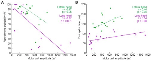
      The authors have slightly misunderstood my comment on "extrapolation": I referred to "environmental extrapolation" in my review without being particularly explicit about my meaning. By "environmental extrapolation", I meant to ask whether the models were predicting to environments that are outside the extent of environments included in the occurrence data used in the manuscript. The authors appear to have understood this to be a comment on geographic extrapolation, or predicting to areas outside the geographic extent included in occurrence data, e.g.: "For H5Nx post-2020, areas of high predicted ecological suitability, such as Brazil, Bolivia, the Caribbean islands, and Jilin province in China, likely result from extrapolations, as these regions reported few or no outbreaks in the training data" (lines 195-197). Is the model extrapolating in environmental space in these regions? This is unclear. I do not suggest that the authors should carry out further analysis, but the multivariate environmental similarly surface (MESS; see Elith et al., 2010: https://doi.org/10.1111/j.2041-210X.2010.00036.x ) is a useful tool to visualise environmental extrapolation and aid model interpretation.

      On the subject of "extrapolation", I am also concerned by the additions at lines 362-370: "...our models extrapolate environmental suitability for H5Nx in wild birds in areas where few or no outbreaks have been reported. This discrepancy may be explained by limited surveillance or underreporting in those regions." The "discrepancy" cited here is a feature of the input dataset, a function of the observation distribution that should be captured in pseudo-absence data. The authors state that Kazakhstan and Central Asia are areas of interest, and that the environments in this region are outside the extent of environments captured in the occurrence dataset, although it is unclear whether "extrapolation" is informed by a quantitative tool like a MESS or judged by some other qualitative test. The authors then cite Australia as an example of a region with some predicted suitability but no HPAI outbreaks to date, however this discussion point is not linked to the idea that the presence of environmental conditions to support transmission need not imply the occurrence of transmission (as in the addition, "...spatial isolation may imply a lower risk of actual occurrences..." at line 214). Ultimately, the authors have not added any clear comment on model uncertainty (e.g., variation between replicated BRTs) as I suggested might be helpful to support their description of model predictions.

      All of my criticisms are, of course, applied with the understanding that niche modelling is imperfect for a disease like HPAI, and that data may be biased/incomplete, etc.: these caveats are common across the niche modelling literature. However, if language around the transmission cycle, the niche, and the interpretation of any of the models is imprecise, which I find it to be in the revised manuscript, it undermines all of the science that is presented in this work.

    3. Reviewer #2 (Public review):

      Summary:

      The geographic range of highly pathogenic avian influenza cases changed substantially around the period 2020, and there is much interest in understanding why. Since 2020 the pathogen irrupted in the Americas and the distribution in Asia changed dramatically. This study aimed to determine which spatial factors (environmental, agronomic and socio-economic) explain the change in numbers and locations of cases reported since 2020 (2020--2023). That's a causal question which they address by applying correlative environmental niche modelling (ENM) approach to the avian influenza case data before (2015--2020) and after 2020 (2020--2023) and separately for confirmed cases in wild and domestic birds. To address their questions they compare the outputs of the respective models, and those of the first global model of the HPAI niche published by Dhingra et al 2016.

      ENM is a correlative approach useful for extrapolating understandings based on sparse geographically referenced observational data over un- or under-sampled areas with similar environmental characteristics in the form of a continuous map. In this case, because the selected covariates about land cover, use, population and environment are broadly available over the entire world, modelled associations between the response and those covariates can be projected (predicted) back to space in the form of a continuous map of the HPAI niche for the entire world.

      Strengths:

      The authors are clear about expected bias in the detection of cases, such geographic variation in surveillance effort (testing of symptomatic or dead wildlife, testing domestic flocks) and in general more detections near areas of higher human population density (because if a tree falls in a forest and there is no-one there, etc), and take steps to ameliorate those. The authors use boosted regression trees to implement the ENM, which typically feature among the best performing models for this application (also known as habitat suitability models). They ran replicate sets of the analysis for each of their model targets (wild/domestic x pathogen variant), which can help produce stable predictions. Their code and data is provided, though I did not verify that the work was reproducible.

      The paper can be read as a partial update to the first global model of H5Nx transmission by Dhingra and others published in 2016 and explicitly follows many methodological elements. Because they use the same covariate sets as used by Dhingra et al 2016 (including the comparisons of the performance of the sets in spatial cross-validation) and for both time periods of interest in the current work, comparison of model outputs is possible. The authors further facilitate those comparisons with clear graphics and supplementary analyses and presentation. The models can also be explored interactively at a weblink provided in text, though it would be good to see the model training data there too.

      The authors' comparison of ENM model outputs generated from the distinct HPAI case datasets is interesting and worthwhile, though for me, only as a response to differently framed research questions.

      Weaknesses:

      This well-presented and technically well-executed paper has one major weakness to my mind. I don't believe that ENM models were an appropriate tool to address their stated goal, which was to identify the factors that "explain" changing HPAI epidemiology.

      Here is how I understand and unpack that weakness:

      (1) Because of their fundamentally correlative nature, ENMs are not a strong candidate for exploring or inferring causal relationships.

      (2) Generating ENMs for a species whose distribution is undergoing broad scale range change is complicated and requires particular caution and nuance in interpretation (e.g., Elith et al, 2010, an important general assumption of environmental niche models is that the target species is at some kind of distributional equilibrium (at time scales relevant to the model application). In practice that means the species has had an opportunity to reach all suitable habitats and therefore its absence from some can be interpreted as either unfavourable environment or interactions with other species). Here data sets for the response (N5H1 or N5Hx case data in domestic or wild birds ) were divided into two periods; 2015--2020, and 2020--2023 based on the rationale that the geographic locations and host-species profile of cases detected in the latter period was suggestive of changed epidemiology. In comparing outputs from multiple ENMs for the same target from distinct time periods the authors are expertly working in, or even dancing around, what is a known grey area, and they need to make the necessary assumptions and caveats obvious to readers.

      (3) To generate global prediction maps via ENM, only variables that exist at appropriate resolution over the desired area can be supplied as covariates. What processes could influence changing epidemiology of a pathogen and are their covariates that represent them? Introduction to a new geographic area (continent) with naive population, immunity in previously exposed populations, control measures to limit spread such as vaccination or destruction of vulnerable populations or flocks? Might those control measures be more or less likely depending on the country as a function of its resources and governance? There aren't globally available datasets that speak to those factors, so the question is not why were they omitted but rather was the authors decision to choose ENMs given their question justified? How valuable are insights based on patterns of correlation change when considering different temporal sets of HPAI cases in relation to a common and somewhat anachronistic set of covariates?

      (4) In general the study is somewhat incoherent with respect to time. Though the case data come from different time periods, each response dataset was modelled separately using exactly the same covariate dataset that predated both sets. That decision should be understood as a strong assumption on the part of the authors that conditions the interpretation: the world (as represented by the covariate set) is immutable, so the model has to return different correlative associations between the case data and the covariates to explain the new data. While the world represented by the selected covariates *may* be relatively stable (could be statistically confirmed), what about the world not represented by the covariates (see point 3)?

      References:

      Dhingra et al, 2016, Global mapping of highly pathogenic avian influenza H5N1 and H5Nx clade 2.3.4.4 viruses with spatial cross-validation, eLife 5, https://doi.org/10.7554/eLife.19571

      Elith, J., Kearney, M., & Phillips, S. (2010). The art of modelling range‐shifting species. Methods in Ecology and Evolution, 1(4), 330-342.

    4. Author response:

      The following is the authors’ response to the current reviews.

      Public Reviews:

      We thank the Reviewers for their thorough attention to our paper and the interesting discussion about the findings. Before responding to more specific comments, here some general points we would like to clarify:

      (1) Ecological niche models are indeed correlative models, and we used them to highlight environmental factors associated with HPAI outbreaks within two host groups. We will further revise the terminology that could still unintentionally suggest causal inference. The few remaining ambiguities were mainly in the Discussion section, where our intent was to interpret the results in light of the broader scientific literature. Particularly, we will change the following expressions:

      -  “Which factors can explain…” to  “Which factors are associated with…” (line 75);

      -  “the environmental and anthropogenic factors influencing” to “the environmental and anthropogenic factors that are correlated with” (line 273);

      -  “underscoring the influence” to “underscoring the strong association” (line 282).

      (2) We respectfully disagree with the suggestion that an ecological niche modelling (ENM) approach is not appropriate for this work and the research question addressed therein. Ecological niche models are specifically designed to estimate the spatial distribution of the environmental suitability of species and pathogens, making them well suited to our research questions. In our study, we have also explicitly detailed the known limitations of ecological niche models in the Discussion section, in line with prior literature, to ensure their appropriate interpretation in the context of HPAI.

      (3) The environmental layers used in our models were restricted to those available at a global scale, as listed in Supplementary Information Resources S1 (https://github.com/sdellicour/h5nx_risk_mapping/blob/master/Scripts_%26_data/SI_Resource_S1.xlsx). Naturally, not all potentially relevant environmental factors could be included, but the selected layers are explicitly documented and only these were assessed for their importance. Despite this limitation, the performance metrics indicate that the models performed well, suggesting that the chosen covariates capture meaningful associations with HPAI occurrence at a global scale.

      Reviewer #1 (Public review):

      The authors aim to predict ecological suitability for transmission of highly pathogenic avian influenza (HPAI) using ecological niche models. This class of models identify correlations between the locations of species or disease detections and the environment. These correlations are then used to predict habitat suitability (in this work, ecological suitability for disease transmission) in locations where surveillance of the species or disease has not been conducted. The authors fit separate models for HPAI detections in wild birds and farmed birds, for two strains of HPAI (H5N1 and H5Nx) and for two time periods, pre- and post-2020. The authors also validate models fitted to disease occurrence data from pre-2020 using post-2020 occurrence data. I thank the authors for taking the time to respond to my initial review and I provide some follow-up below.

      Detailed comments:

      In my review, I asked the authors to clarify the meaning of "spillover" within the HPAI transmission cycle. This term is still not entirely clear: at lines 409-410, the authors use the term with reference to transmission between wild birds and farmed birds, as distinct to transmission between farmed birds. It is implied but not explicitly stated that "spillover" is relevant to the transmission cycle in farmed birds only. The sentence, "we developed separate ecological niche models for wild and domestic bird HPAI occurrences ..." could have been supported by a clear sentence describing the transmission cycle, to prime the reader for why two separate models were necessary.

      We respectfully disagree that the term “spillover” is unclear in the manuscript. In both the Methods and Discussion sections (lines 387-391 and 409-414), we explicitly define “spillover” as the introduction of HPAI viruses from wild birds into domestic poultry, and we distinguish this from secondary farm-to-farm transmission. Our use of separate ecological niche models for wild and domestic outbreaks reflects not only the distinction between primary spillover and secondary transmission, but also the fundamentally different ecological processes, surveillance systems, and management implications that shape outbreaks in these two groups. We will clarify this choice in the revised manuscript when introducing the separate models. Furthermore, on line 83, we will add “as these two groups are influenced by different ecological processes, surveillance biases, and management contexts”.

      I also queried the importance of (dead-end) mammalian infections to a model of the HPAI transmission risk, to which the authors responded: "While spillover events of HPAI into mammals have been documented, these detections are generally considered dead-end infections and do not currently represent sustained transmission chains. As such, they fall outside the scope of our study, which focuses on avian hosts and models ecological suitability for outbreaks in wild and domestic birds." I would argue that any infections, whether they are in dead-end or competent hosts, represent the presence of environmental conditions to support transmission so are certainly relevant to a niche model and therefore within scope. It is certainly understandable if the authors have not been able to access data of mammalian infections, but it is an oversight to dismiss these infections as irrelevant.

      We understand the Reviewer’s point, but our study was designed to model HPAI occurrence in avian hosts only. We therefore restricted our analysis to wild birds and domestic poultry, which represent the primary hosts for HPAI circulation and the focus of surveillance and control measures. While mammalian detections have been reported, they are outside the scope of this work.

      Correlative ecological niche models, including BRTs, learn relationships between occurrence data and covariate data to make predictions, irrespective of correlations between covariates. I am not convinced that the authors can make any "interpretation" (line 298) that the covariates that are most informative to their models have any "influence" (line 282) on their response variable. Indeed, the observation that "land-use and climatic predictors do not play an important role in the niche ecological models" (line 286), while "intensive chicken population density emerges as a significant predictor" (line 282) begs the question: from an operational perspective, is the best (e.g., most interpretable and quickest to generate) model of HPAI risk a map of poultry farming intensity?

      We agree that poultry density may partly reflect reporting bias, but we also assumed it a meaningful predictor of HPAI risk. Its importance in our models is therefore expected. Importantly, our BRT framework does more than reproduce poultry distribution: it captures non-linear relationships and interactions with other covariates, allowing a more nuanced characterisation of risk than a simple poultry density map. Note also that we distinguished in our models intensive and extensive chicken poultry density and duck density. Therefore, it is not a “map of poultry farming intensity”. 

      At line 282, we used the word “influence” while fully recognising that correlative models cannot establish causality. Indeed, in our analyses, “relative influence” refers to the importance metric produced by the BRT algorithm (Ridgeway, 2020), which measures correlative associations between environmental factors and outbreak occurrences. These scores are interpreted in light of the broader scientific literature, therefore our interpretations build on both our results and existing evidence, rather than on our models alone. However, in the next version of the paper, we will revise the sentence as: “underscoring the strong association of poultry farming practices with HPAI spread (Dhingra et al., 2016)”. 

      I have more significant concerns about the authors' treatment of sampling bias: "We agree with the Reviewer's comment that poultry density could have potentially been considered to guide the sampling effort of the pseudo-absences to consider when training domestic bird models. We however prefer to keep using a human population density layer as a proxy for surveillance bias to define the relative probability to sample pseudo-absence points in the different pixels of the background area considered when training our ecological niche models. Indeed, given that poultry density is precisely one of the predictors that we aim to test, considering this environmental layer for defining the relative probability to sample pseudo-absences would introduce a certain level of circularity in our analytical procedure, e.g. by artificially increasing to influence of that particular variable in our models." The authors have elected to ignore a fundamental feature of distribution modelling with occurrence-only data: if we include a source of sampling bias as a covariate and do not include it when we sample background data, then that covariate would appear to be correlated with presence. They acknowledge this later in their response to my review: "...assuming a sampling bias correlated with poultry density would result in reducing its effect as a risk factor." In other words, the apparent predictive capacity of poultry density is a function of how the authors have constructed the sampling bias for their models. A reader of the manuscript can reasonably ask the question: to what degree are is the model a model of HPAI transmission risk, and to what degree is the model a model of the observation process? The sentence at lines 474-477 is a helpful addition, however the preceding sentence, "Another approach to sampling pseudo-absences would have been to distribute them according to the density of domestic poultry," (line 474) is included without acknowledgement of the flow-on consequence to one of the key findings of the manuscript, that "...intensive chicken population density emerges as a significant predictor..." (line 282). The additional context on the EMPRES-i dataset at line 475-476 ("the locations of outbreaks ... are often georeferenced using place name nomenclatures") is in conflict with the description of the dataset at line 407 ("precise location coordinates"). Ultimately, the choices that the authors have made are entirely defensible through a clear, concise description of model features and assumptions, and precise language to guide the reader through interpretation of results. I am not satisfied that this is provided in the revised manuscript.

      We thank the Reviewer for this important point. To address it, we compared model predictive performance and covariate relative influences obtained when pseudo-absences were weighted by poultry density versus human population density (Author response table 1). The results show that differences between the two approaches are marginal, both in predictive performance (ΔAUC ranging from -0.013 to +0.002) and in the ranking of key predictors (see below Author response images 1 and 2). For instance, intensive chicken density consistently emerged as an important predictor regardless of the bias layer used.

      Note: the comparison was conducted using a simplified BRT configuration for computational efficiency (fewer trees, fixed 5-fold random cross-validation, and standardised parameters). Therefore, absolute values of AUC and variable importance may differ slightly from those in the manuscript, but the relative ranking of predictors and the overall conclusions remain consistent.

      Given these small differences, we retained the approach using human population density. We agree that poultry density partly reflects surveillance bias as well as true epidemiological risk, and we will clarify this in the revised manuscript by noting that the predictive role of poultry density reflects both biological processes and surveillance systems. Furthermore, on line 289, we will add “We note, however, that intensive poultry density may reflect both surveillance intensity and epidemiological risk, and its predictive role in our models should be interpreted in light of both processes”.

      Author response table 1.

      Comparison of model predictive performances (AUC) between pseudo-absence sampling were weighted by poultry density and by human population density across host groups, virus types, and time periods. Differences in AUC values are shown as the value for poultry-weighted minus human-weighted pseudo-absences.

      Author response image 1.

      Comparison of variable relative influence (%) between models trained with pseudo-absences weighted by poultry density (red) and human population density (blue) for domestic bird outbreaks. Results are shown for four datasets: H5N1 (<2020), H5N1 (>2020), H5Nx (<2020), and H5Nx (>2020).

      Author response image 2.

      Comparison of variable relative influence (%) between models trained with pseudo-absences weighted by poultry density (red) and human population density (blue) for wild bird outbreaks. Results are shown for three datasets: H5N1 (>2020), H5Nx (<2020), and H5Nx (>2020).

      The authors have slightly misunderstood my comment on "extrapolation": I referred to "environmental extrapolation" in my review without being particularly explicit about my meaning. By "environmental extrapolation", I meant to ask whether the models were predicting to environments that are outside the extent of environments included in the occurrence data used in the manuscript. The authors appear to have understood this to be a comment on geographic extrapolation, or predicting to areas outside the geographic extent included in occurrence data, e.g.: "For H5Nx post-2020, areas of high predicted ecological suitability, such as Brazil, Bolivia, the Caribbean islands, and Jilin province in China, likely result from extrapolations, as these regions reported few or no outbreaks in the training data" (lines 195-197). Is the model extrapolating in environmental space in these regions? This is unclear. I do not suggest that the authors should carry out further analysis, but the multivariate environmental similarly surface (MESS; see Elith et al., 2010) is a useful tool to visualise environmental extrapolation and aid model interpretation.

      On the subject of "extrapolation", I am also concerned by the additions at lines 362-370: "...our models extrapolate environmental suitability for H5Nx in wild birds in areas where few or no outbreaks have been reported. This discrepancy may be explained by limited surveillance or underreporting in those regions." The "discrepancy" cited here is a feature of the input dataset, a function of the observation distribution that should be captured in pseudo-absence data. The authors state that Kazakhstan and Central Asia are areas of interest, and that the environments in this region are outside the extent of environments captured in the occurrence dataset, although it is unclear whether "extrapolation" is informed by a quantitative tool like a MESS or judged by some other qualitative test. The authors then cite Australia as an example of a region with some predicted suitability but no HPAI outbreaks to date, however this discussion point is not linked to the idea that the presence of environmental conditions to support transmission need not imply the occurrence of transmission (as in the addition, "...spatial isolation may imply a lower risk of actual occurrences..." at line 214). Ultimately, the authors have not added any clear comment on model uncertainty (e.g., variation between replicated BRTs) as I suggested might be helpful to support their description of model predictions.

      Many thanks for the clarification. Indeed, we interpreted your previous comments in terms of geographic extrapolations. We thank the Reviewer for these observations. We will adjust the wording to further clarify that predictions of ecological suitability in areas with few or no reported outbreaks (e.g., Central Asia, Australia) are not model errors but expected extrapolations, since ecological suitability does not imply confirmed transmission (for instance, on Line 362: “our models extrapolate environmental suitability” will be changed to “Interestingly, our models extrapolate geographical”). These predictions indicate potential environments favorable to circulation if the virus were introduced.

      In our study, model uncertainty is formally assessed when comparing the predictive performances of our models (Fig. S3, Table S1), the relative influence (Table S3) and response curves (Fig. 2) associated with each environmental factor (Table S2). All the results confirming a good converge between these replicates. Finally, we indeed did not use a quantitative tool such as a MESS to assess extrapolation but did rely on qualitative interpretation of model outputs.

      All of my criticisms are, of course, applied with the understanding that niche modelling is imperfect for a disease like HPAI, and that data may be biased/incomplete, etc.: these caveats are common across the niche modelling literature. However, if language around the transmission cycle, the niche, and the interpretation of any of the models is imprecise, which I find it to be in the revised manuscript, it undermines all of the science that is presented in this work.

      We respectfully disagree with this comment. The scope of our study and the methods employed are clearly defined in the manuscript, and the limitations of ecological niche modelling in this context are explicitly acknowledged in the Discussion section. While we appreciate the Reviewer’s concern, the comment does not provide specific examples of unclear or imprecise language regarding the transmission cycle, niche, or interpretation of the models. Without such examples, it is difficult to identify further revisions that would improve clarity.

      Reviewer #2 (Public review):

      The geographic range of highly pathogenic avian influenza cases changed substantially around the period 2020, and there is much interest in understanding why. Since 2020 the pathogen irrupted in the Americas and the distribution in Asia changed dramatically. This study aimed to determine which spatial factors (environmental, agronomic and socio-economic) explain the change in numbers and locations of cases reported since 2020 (2020--2023). That's a causal question which they address by applying correlative environmental niche modelling (ENM) approach to the avian influenza case data before (2015--2020) and after 2020 (2020--2023) and separately for confirmed cases in wild and domestic birds. To address their questions they compare the outputs of the respective models, and those of the first global model of the HPAI niche published by Dhingra et al 2016.

      We do not agree with this comment. In the manuscript, it is well established that we are quantitatively assessing factors that are associated with occurrences data before and after 2020. We do not claim to determine the causality. One sentence of the Introduction section (lines 75-76) could be confusing, so we intend to modify it in the final revision of our manuscript. 

      ENM is a correlative approach useful for extrapolating understandings based on sparse geographically referenced observational data over un- or under-sampled areas with similar environmental characteristics in the form of a continuous map. In this case, because the selected covariates about land cover, use, population and environment are broadly available over the entire world, modelled associations between the response and those covariates can be projected (predicted) back to space in the form of a continuous map of the HPAI niche for the entire world.

      We fully agree with this assessment of ENM approaches.

      Strengths:

      The authors are clear about expected bias in the detection of cases, such geographic variation in surveillance effort (testing of symptomatic or dead wildlife, testing domestic flocks) and in general more detections near areas of higher human population density (because if a tree falls in a forest and there is no-one there, etc), and take steps to ameliorate those. The authors use boosted regression trees to implement the ENM, which typically feature among the best performing models for this application (also known as habitat suitability models). They ran replicate sets of the analysis for each of their model targets (wild/domestic x pathogen variant), which can help produce stable predictions. Their code and data is provided, though I did not verify that the work was reproducible.

      The paper can be read as a partial update to the first global model of H5Nx transmission by Dhingra and others published in 2016 and explicitly follows many methodological elements. Because they use the same covariate sets as used by Dhingra et al 2016 (including the comparisons of the performance of the sets in spatial cross-validation) and for both time periods of interest in the current work, comparison of model outputs is possible. The authors further facilitate those comparisons with clear graphics and supplementary analyses and presentation. The models can also be explored interactively at a weblink provided in text, though it would be good to see the model training data there too.

      The authors' comparison of ENM model outputs generated from the distinct HPAI case datasets is interesting and worthwhile, though for me, only as a response to differently framed research questions.

      Weaknesses:

      This well-presented and technically well-executed paper has one major weakness to my mind. I don't believe that ENM models were an appropriate tool to address their stated goal, which was to identify the factors that "explain" changing HPAI epidemiology.

      Here is how I understand and unpack that weakness:

      (1) Because of their fundamentally correlative nature, ENMs are not a strong candidate for exploring or inferring causal relationships.

      (2) Generating ENMs for a species whose distribution is undergoing broad scale range change is complicated and requires particular caution and nuance in interpretation (e.g., Elith et al, 2010, an important general assumption of environmental niche models is that the target species is at some kind of distributional equilibrium (at time scales relevant to the model application). In practice that means the species has had an opportunity to reach all suitable habitats and therefore its absence from some can be interpreted as either unfavourable environment or interactions with other species). Here data sets for the response (N5H1 or N5Hx case data in domestic or wild birds ) were divided into two periods; 2015--2020, and 2020--2023 based on the rationale that the geographic locations and host-species profile of cases detected in the latter period was suggestive of changed epidemiology. In comparing outputs from multiple ENMs for the same target from distinct time periods the authors are expertly working in, or even dancing around, what is a known grey area, and they need to make the necessary assumptions and caveats obvious to readers.

      We thank the Reviewer for this observation. First, we constrained pseudo-absence sampling to countries and regions where outbreaks had been reported, reducing the risk of interpreting non-affected areas as environmentally unsuitable. Second, we deliberately split the outbreak data into two periods (2015-2020 and 2020-2023) because we do not assume a single stable equilibrium across the full study timeframe. This division reflects known epidemiological changes around 2020 and allows each period to be modeled independently. Within each period, ENM outputs are interpreted as associations between outbreaks and covariates, not as equilibrium distributions. Finally, by testing prediction across periods, we assessed both niche stability and potential niche shifts. These clarifications will be added to the manuscript to make our assumptions and limitations explicit.

      Line 66, we will add: “Ecological niche model outputs for range-shifting pathogens must therefore be interpreted with caution (Elith et al., 2010). Despite this limitation, correlative ecological niche models  remain useful for identifying broad-scale associations and potential shifts in distribution. To account for this, we analysed two distinct time periods (2015-2020 and 2020-2023).”

      Line 123, we will revise “These findings underscore the ability of pre-2020 models in forecasting the recent geographic distribution of ecological suitability for H5Nx and H5N1 occurrences” to “These results suggest that pre-2020 models captured broad patterns of suitability for H5Nx and H5N1 outbreaks, while post-2020 models provided a closer fit to the more recent epidemiological situation”.

      (3) To generate global prediction maps via ENM, only variables that exist at appropriate resolution over the desired area can be supplied as covariates. What processes could influence changing epidemiology of a pathogen and are their covariates that represent them? Introduction to a new geographic area (continent) with naive population, immunity in previously exposed populations, control measures to limit spread such as vaccination or destruction of vulnerable populations or flocks? Might those control measures be more or less likely depending on the country as a function of its resources and governance? There aren't globally available datasets that speak to those factors, so the question is not why were they omitted but rather was the authors decision to choose ENMs given their question justified? How valuable are insights based on patterns of correlation change when considering different temporal sets of HPAI cases in relation to a common and somewhat anachronistic set of covariates?

      We agree that the ecological niche models trained in our study are limited to environmental and host factors, as described in the Methods section with the selection of predictors. While such models cannot capture causality or represent processes such as immunity, control measures, or governance, they remain a useful tool for identifying broad associations between outbreak occurrence and environmental context. Our study cannot infer the full mechanisms driving changes in HPAI epidemiology, but it does provide a globally consistent framework to examine how associations with available covariates vary across time periods.

      (4) In general the study is somewhat incoherent with respect to time. Though the case data come from different time periods, each response dataset was modelled separately using exactly the same covariate dataset that predated both sets. That decision should be understood as a strong assumption on the part of the authors that conditions the interpretation: the world (as represented by the covariate set) is immutable, so the model has to return different correlative associations between the case data and the covariates to explain the new data. While the world represented by the selected covariates *may* be relatively stable (could be statistically confirmed), what about the world not represented by the covariates (see point 3)?

      We used the same covariate layers for both periods, which indeed assumes that these environmental and host factors are relatively stable at the global scale over the short timeframe considered. We believe this assumption is reasonable, as poultry density, land cover, and climate baselines do not change drastically between 2015 and 2023 at the resolution of our analysis. We agree, however, that unmeasured processes such as control measures, immunity, or governance may have changed during this time and are not captured by our covariates.

      Recommendations for the Authors:

      Reviewer #1 (Recommendations for the authors):

      - Line 400-401: "over the 2003-2016 periods" has an extra "s"; "two host species" (with reference to wild and domestic birds) would be more precise as "two host groups".

      - Remove comma line 404

      Many thanks for these comments, we have modified the text accordingly.

      Reviewer #2 (Recommendations for the authors):

      Most of my work this round is encapsulated in the public part of the review.

      The authors responded positively to the review efforts from the previous round, but I was underwhelmed with the changes to the text that resulted. Particularly in regard to limiting assumptions - the way that they augmented the text to refer to limitations raised in review downplayed the importance of the assumptions they've made. So they acknowledge the significance of the limitation in their rejoinder, but in the amended text merely note the limitation without giving any sense of what it means for their interpretation of the findings of this study.

      The abstract and findings are essentially unchanged from the previous draft.

      I still feel the near causal statements of interpretation about the covariates are concerning. These models really are not a good candidate for supporting the inference that they are making and there seem to be very strong arguments in favour of adding covariates that are not globally available.

      We never claimed causal interpretation, and we have consistently framed our analyses in terms of associations rather than mechanisms. We acknowledge that one phrasing in the research questions (“Which factors can explain…”) could be misinterpreted, and we are correcting this in the revised version to read “Which factors are associated with…”. Our approach follows standard ecological niche modelling practice, which identifies statistical associations between occurrence data and covariates. As noted in the Discussion section, these associations should not be interpreted as direct causal mechanisms. Finally, all interpretive points in the manuscript are supported by published literature, and we consider this framing both appropriate and consistent with best practice in ecological niche modelling (ENM) studies.

      We assessed predictor contributions using the “relative influence” metric, the terminology reported by the R package “gbm” (Ridgeway, 2020). This metric quantifies the contribution of each variable to model fit across all trees, rescaled to sum to 100%, and should be interpreted as an association rather than a causal effect.

      L65-66 The general difficulty of interpreting ENM output with range-shifting species should be cited here to alert readers that they should not blithely attempt what follows at home.

      I believe that their analysis is interesting and technically very well executed, so it has been a disappointment and hard work to write this assessment. My rough-cut last paragraph of a reframed intro would go something like - there are many reasons in the literature not to do what we are about to do, but here's why we think it can be instructive and informative, within certain guardrails.

      To acknowledge this comment and the previous one, we revised lines 65-66 to: “However, recent outbreaks raise questions about whether earlier ecological niche models still accurately predict the current distribution of areas ecologically suitable for the local circulation of HPAI H5 viruses. Ecological niche model outputs for range-shifting pathogens must therefore be interpreted with caution (Elith et al., 2010). Despite this limitation, correlative ecological niche models  remain useful for identifying broad-scale associations and potential shifts in distribution.”

      We respectfully disagree with the Reviewer’s statement that “_there are many reasons in the literature not to do what we are about to do”._ All modeling approaches, including mechanistic ones, have limitations, and the literature is clear on both the strengths and constraints of ecological niche models. Our manuscript openly acknowledges these limits and frames our findings accordingly. We therefore believe that our use of an ENM approach is justified and contributes valuable insights within these well-defined boundaries.

      Reference: Ridgeway, G. (2007). Generalized Boosted Models: A guide to the gbm package. Update, 1(1), 2007.


      The following is the authors’ response to the original reviews.

      Reviewer #1(Public review):

      I am concerned by the authors' conceptualisation of "niche" within the manuscript. Is the "niche" we are modelling the niche of the pathogen itself? The niche of the (wild) bird host species as a group? The niche of HPAI transmission within (wild) bird host species (i.e., an intersection of pathogen and bird niches)? Or the niche of HPAI transmission in poultry? The precise niche being modelled should be clarified in the Introduction or early in the Methods of the manuscript. The first two definitions of niche listed above are relevant, but separate from the niche modelled in the manuscript - this should be acknowledged.

      We acknowledge that these concepts were probably not enough clearly defined in the previous version of our manuscript, and we have now included an explicit definition in the fourth paragraph of the Introduction section: “We developed separate ecological niche models for wild and domestic bird HPAI occurrences, these models thus predicting the ecological suitability for the risk of local viral circulation leading to the detection of HPAI occurrences within each host group (rather than the niche of the virus or the host species alone).”

      The authors should consider the precise transmission cycle involved in each HPAI case: "index cases" in farmed poultry, caused by "spillover" from wild birds, are relevant to the wildlife transmission cycle, while the ecological conditions coinciding with subsequent transmission in farmed poultry are likely to be fundamentally different. (For example, subsequent transmission is not conditional on the presence of wild birds.) Modelling these two separate, but linked, transmission cycles together may omit important nuances from the modelling framework.

      We thank the Reviewer for highlighting the distinction between primary (wild-todomestic) and secondary (farm-to-farm) transmission cycles. Our modelling framework was designed to assess the ecological suitability of HPAI occurrences in wild and domestic birds separately. In the domestic poultry models, the response variables are the confirmed outbreaks data and do not distinguish between index cases resulting from primary or secondary infections.

      One of the aims of the study is to evaluate the spatial distribution of areas ecologically suitable for local H5N1/x circulation either leading to domestic or wild bird cases, i.e. to identify environmental conditions where the virus may have persisted or spread, whether as a result of introduction by wild birds or farm-to-farm transmission. Introducing mechanistic distinctions in the response variable would not necessarily improve or affect the ecological suitability maps, since each type of transmission is likely to be associated with different covariates that are included in the models.

      Also, the EMPRES-i database does not indicate whether each record corresponds to an index case or a secondary transmission event, so in practice it would not be possible to produce two different models. However, we agree that distinguishing between types of transmission is an interesting perspective for future research. This could be explored, for example, by mapping interfaces between wild and domestic bird populations or by inferring outbreak transmission trees using genomic data when available.

      To avoid confusion, we now explicitly clarify this aspect in the Materials and Methods section: “It is important to note that the EMPRES-i database does not distinguish between index cases (e.g., primary spillover from wild birds) and secondary farm-to-farm transmissions. As such, our ecological niche models are trained on confirmed HPAI outbreaks in poultry that may result from different transmission dynamics — including both initial introduction events influenced by environmental factors and subsequent spread within poultry systems.”

      We now also address this limitation in the Discussion section: “Finally, our models for domestic poultry do not distinguish between primary introduction events (e.g., spillover from wild birds) and secondary transmission between farms due to limitations in the available surveillance data. While environmental factors likely influence the risk of initial spillover events, secondary spread is more often driven by anthropogenic factors such as biosecurity practices and poultry trade, which are not included in our current modelling framework.”

      The authors should clarify the meaning of "spillover" within the HPAI transmission cycle: if spillover transmission is from wild birds to farmed poultry, then subsequent transmission in poultry is separate from the wildlife transmission cycle. This is particularly relevant to the Discussion paragraph beginning at line 244: does "farm to farm transmission" have a distinct ecological niche to transmission between wild birds, and transmission between wild birds and farmed birds? And while there has been a spillover of HPAI to mammals, could the authors clarify that these detections are dead-end? And not represented in the dataset? Dhingra et al., 2016 comment on the contrast between models of "directly transmitted" pathogens, such as HPAI, and vector-borne diseases: for vector-borne diseases, "clear eco-climatic boundaries of vectors can be mapped", whereas "HPAI is probably not as strongly environmentally constrained". This is an important piece of nuance in their Discussion and a comment to a similar effect may be of use in this manuscript.

      Following the Reviewer’s previous comment, we have now added clarifications in the Methods and Discussion sections defining spillover as the transmission of HPAI viruses from wild birds to domestic poultry (index cases), and secondary transmission as onward spread between farms. As mentioned in our answer above, we now emphasise that our models do not distinguish these dynamics, which are likely to be influenced by different drivers — ecological in the case of spillover, and often anthropogenic (e.g., poultry trade movement, biosecurity) in the case of farm-to-farm transmission.

      The discussion regarding farm-to-farm transmission and spillovers is indeed an interpretation derived from the covariates analysis (see the second paragraph in the Discussion section). Specifically, we observed a stronger association between HPAI occurrences and domestic bird density after 2020, which may suggest that secondary infections (e.g., farm-to-farm transmission) became more prominent or more frequently reported. We however acknowledge that our data do not allow us to distinguish primary introductions from secondary transmission events, and we have added a sentence to explicitly clarify this: “However, this remains an interpretation, as the available data do not allow us to distinguish between index cases and secondary transmission events.”

      We thank the Reviewer for raising the point of mammalian infections. While spillover events of HPAI into mammals have been documented, these detections are generally considered dead-end infections and do not currently represent sustained transmission chains. As such, they fall outside the scope of our study, which focuses on avian hosts and models ecological suitability for outbreaks in wild and domestic birds. However, we agree that future work could explore the spatial overlap between mammalian outbreak detections and ecological suitability maps for wild birds to assess whether such spillovers may be linked to localised avian transmission dynamics.

      Finally, we have added a comment about the differences between pathogens strongly constrained by the environments and HPAI: “This suggests that HPAI H5Nx is not as strongly environmentally constrained as vector-borne pathogens, for which clear eco-climatic boundaries (e.g., vector borne diseases) can be mapped (Dhingra et al., 2016).” This aligns with the interpretation provided by Dhingra and colleagues (2016) and helps contextualise the predictive limitations of ecological niche models for directly transmitted pathogens like HPAI.

      There are several places where some simple clarification of language could answer my questions related to ecological niches. For example, on line 74, "the ecological niche" should be followed by "of the pathogen", or "of HPAI transmission in wild birds", or some other qualifier that is most appropriate to the Authors' conceptualisation of the niche modelled in the manuscript. Similarly, in the following sentence, "areas at risk" could be followed by "of transmission in wild birds", to make the transmission cycle that is the subject of modelling clear to the reader. On line 83, it is not clear who or what is the owner of "their ecological niches": is this "poultry and wild birds", or the pathogen?

      We agree with that suggestion and have now modified the related part of the text  accordingly (e.g., “areas at risk for local HPAI circulation” and “of HPAI in wild or domestic birds”).

      I am concerned by the authors' treatment of sampling bias in their BRT modelling framework. If we are modelling the niche of HPAI transmission, we would expect places that are more likely to be subject to disease surveillance to be represented in the set of locations where the disease has been detected. I do not agree that pseudo-absence points are sampled "to account for the lack of virus detection in some areas" - this description is misleading and does not match the following sentence ("pseudo-absence points sampled ... to reflect the greater surveillance efforts ..."). The distribution of pseudo-absences should aim to capture the distribution of probable disease surveillance, as these data act as a stand-in for missing negative surveillance records. It is sensible that pseudo-absences for disease detection in wild birds are sampled proportionately to human population density, as the disease is detected in dead wild birds, which are more likely to be identified close to areas of human occupation (as stated on line 163). However, I do not agree that the same applies to poultry - the density of farmed poultry is likely to be a better proxy for surveillance intensity in farmed birds. Human population density and farmed poultry density may be somewhat correlated (i.e., both are low in remote areas), but poultry density is likely to be higher in rural areas, which are assumed to have relatively lower surveillance intensity under the current approach. The authors allude to this in the Discussion: "monitoring areas with high intensive chicken densities ... remains crucial for the early detection and management of HPAI outbreaks".

      We agree with the Reviewer's comment that poultry density could have potentially been considered to guide the sampling effort of the pseudo-absences to consider when training domestic bird models. We however prefer to keep using a human population density layer as a proxy for surveillance bias to define the relative probability to sample pseudoabsence points in the different pixels of the background area considered when training our ecological niche models. Indeed, given that poultry density is precisely one of the predictors that we aim to test, considering this environmental layer for defining the relative probability to sample pseudo-absences would introduce a certain level of circularity in our analytical procedure, e.g. by artificially increasing to influence of that particular variable in our models.

      Furthermore, it is also worth noting that, to better account for variations in surveillance intensity, we also adjusted the sampling effort by allocating pseudo-absences in proportion to the number of confirmed outbreaks per administrative unit (country or sub-national regions for Russia and China). This approach aimed to reduce bias caused by uneven reporting and surveillance efforts between regions. Additionally, we restricted model training to countries or regions with a minimum surveillance threshold (at least five confirmed outbreaks per administrative unit). Therefore, both presence and pseudo-absence points originated from areas with more consistent surveillance data.

      We acknowledge in the Materials and Methods section that the approach proposed by the Reviewer could have been used: “Another approach to sampling pseudo-absences would have been to distribute them according to the density of domestic poultry.” Finally, our approach is also justified in our response to the next comment of the Reviewer.

      Having written my review, including the paragraph above, I briefly scanned Dhingra et al., and found that they provide justification for the use of human population density to sample pseudoabsences in farmed birds: "the Empres-i database compiles outbreak locations data from very heterogeneous sources and in the absence of explicit GPS location data, the geo-referencing of individual cases is often through the use of place name gazetteers that will tend to force the outbreak location populated place, rather in the exact location of the farm where the disease was found, which would introduce a bias correlated with human population density." This context is entirely missing from the manuscript under review, however, I maintain the comment in the paragraph above - have the Authors trialled sampling pseudo-absences from poultry density layers?

      We agree with the Reviewer’s comment and have now added this precision in the Materials and Methods section (in the third paragraph dedicated to ecological niche modelling): “However, as pointed out by Dhingra and colleagues (2016), the locations of outbreaks in the EMPRES-i database are often georeferenced using place name nomenclatures due to a lack of accurate GPS data, which could introduce a spatial bias towards populated areas.”

      The authors indirectly acknowledge the role of sampling bias in model predictions at line 163, however, this point could be clearer: there is sampling bias in the set of locations where HPAI has been observed and failure to adequately replicate this sampling bias in pseudo-absence data could lead covariates that are correlated with the observation distribution to appear to be correlated with the target distribution. This point is alluded to but should be clearly acknowledged to allow the reader to appropriately interpret your results. I understand the point being made on line 163 is that surveillance of HPAI in wild birds has become more structured and less opportunistic over time - if this is the case, a statement to this effect could replace "which could influence earlier data sets", which is a little ambiguous. The Authors acknowledge the role of sampling bias in lines 241-242 - this may be a good place to remind the reader that they have attempted to incorporate sampling bias through the selection of their pseudoabsence dataset, particularly for wild bird models.

      We thank the Reviewer for this comment. We have now clarified in the text that observed data on HPAI occurrence are inherently influenced by heterogeneous surveillance efforts and that failure to replicate this bias in pseudo-absence sampling could effectively lead to misleading correlations with covariates associated with surveillance effort rather than true ecological suitability. We have now rephrased the related sentence as follows: “This decline may indicate a reduced bias in observation data: typically, dead wild birds are more frequently found near human-populated areas due to opportunistic detections, whereas more recent surveillance efforts have become increasingly proactive (Giacinti et al., 2024).”

      Dhingra et al. aimed to account for the effect of mass vaccination of birds in China. This does not appear to be included in the updated models - is this a relevant covariate to consider in updated models? Are the models trained on pre-2020 data predicting to post-2020 given the same presence dataset as previous models? It may be helpful to provide a comment on this if we consider the pre-2020 models in this work to be representative of pre-2020 models as a cohort. Given the framing of the manuscript as an update to Dhingra et al., it may be useful for the authors to briefly summarise any differences between the existing models and updated models. Dhingra et al., also examine spatial extrapolation, which is not addressed here. Environmental extrapolation may be a useful metric to consider: are there areas where models are extrapolating that are predicted to be at high risk of HPAI transmission? Finally, they also provide some inset panels on global maps of model predictions - something similar here may also be useful.

      We thank the Reviewer for these comments. Vaccination coverage is indeed a relevant covariate for HPAI suitability in domestic birds. However, we did not include this variable in our updated models for two reasons. First, comprehensive vaccination data were only available for China, so it is not possible to include this variable in a global model. Second, available data were outdated and vaccination strategies can vary substantially over time.

      We however agree with the Reviewer that the Materials and Methods section did not clarify clearly the differences with Dhingra et al. (2016), and we now detail these differences at the beginning of the Materials and Methods section: “Our approach is similar to the one implemented by Dhingra and colleagues (2016). While Dhingra et al. (2016) developed their models only for domestic birds over the 2003-2016 periods, our models were developed for two host species separately (wild and domestic birds) and for two time periods (2016-2020 and 2020-2023).”

      We also detail the main difference concerning the pseudo-absences sampling:  Dhingra and colleagues (2016) used human population density to sample pseudo-absences to reflect potential surveillance bias and also account for spatial filtering (min/max distances from presence). We adopted a similar strategy but also incorporated outbreak count per country or province (in the case of China and Russia) into the pseudo-absence sampling process to further account for within-country surveillance heterogeneity. We have now added these specifications in the Materials and Methods section: “To account for heterogeneity in AIV surveillance and minimise the risk of sampling pseudo-absences in poorly monitored regions, we restricted our analysis to countries (or administrative level 1 units in China and Russia) with at least five confirmed outbreaks. Unlike Dhingra et al. (2016), who sampled pseudoabsences across a broader global extent, our sampling was limited to regions with demonstrated surveillance activity. In addition, we adjusted the density of pseudo-absence points according to the number of reported outbreaks in each country or admin-1 unit, as a proxy for surveillance effort — an approach not implemented in this previous study.”

      We have now also provided a comparison between the different outputs, particularly in the Results section: “Our findings were overall consistent with those previously reported by Dhingra and colleagues (Dhingra et al., 2016), who used data from January 2004 to March 2015 for domestic poultry. However, some differences were noted: their maps identified higher ecological suitability for H5 occurrences before 2016 in North America, West Africa, eastern Europe, and Bangladesh, while our maps mainly highlight ecologically suitable regions in China, South-East Asia, and Europe (Fig. S5). In India, analyses consistently identified high ecologically suitable areas for the risk of local H5Nx and H5N1 circulation for the three time periods (pre-2016, 2016-2020, and post-2020). Similar to the results reported by Dhingra and colleagues, we observed an increase in the ecological suitability estimated for H5N1 occurrence in South America's domestic bird populations post-2020. Finally, Dhingra and colleagues identified high suitability areas for H5Nx occurrence in North America, which are predicted to be associated with a low ecological suitability in the 2016-2020 models.”

      We acknowledge that some regions predicted as highly suitable correspond to areas where extrapolation likely occurs due to limited or no recorded outbreaks. We have now added these specifications when discussing the resulting suitability maps obtained for domestic birds: “For H5Nx post-2020, areas of high predicted ecological suitability, such as Brazil, Bolivia, the Caribbean islands, and Jilin province in China, likely result from extrapolations, as these regions reported few or no outbreaks in the training data”, and, for wild birds: “Some of the areas with high predicted ecological suitability reflect the result of extrapolations. This is particularly the case in coastal regions of West and North Africa, the Nile Basin, Central Asia (Kyrgyzstan, Tajikistan, Uzbekistan), Brazil (including the Amazon and coastal areas), southern Australia, and the Caribbean, where ecological conditions are similar to those in areas where outbreaks are known to occur but where records of outbreaks are still rare.”

      For wild birds (H5Nx, post-2020), high ecological suitability was predicted along the West and North African coasts, the Nile basin, Central Asia (e.g., Kyrgyzstan, Tajikistan, Uzbekistan), the Brazilian coast and Amazon region, Caribbean islands, southern Australia, and parts of Southeast Asia. Ecological suitability estimated in these regions may directly result from extrapolations and should therefore be interpreted cautiously.

      We also added a discussion of the extrapolation for wild birds (in the Discussion section): “Interestingly, our models extrapolate environmental suitability for H5Nx in wild birds in areas where few or no outbreaks have been reported. This discrepancy may be explained by limited surveillance or underreporting in those regions. For instance, there is significant evidence that Kazakhstan and Central Asia play a role as a centre for the transmission of avian influenza viruses through migratory birds (Amirgazin et al., 2022; FAO, 2005; Sultankulova et al., 2024). However, very few wild bird cases are reported in EMPRES-i. In contrast, Australia appears environmentally suitable in our models, yet no incursion of HPAI H5N1 2.3.4.4b has occurred despite the arrival of millions of migratory shorebirds and seabirds from Asia and North America. Extensive surveillance in 2022 and 2023 found no active infections nor evidence of prior exposure to the 2.3.4.4b lineage (Wille et al., 2024; Wille and Klaassen, 2023).”

      We agree that inset panels can be helpful for visualising global patterns. However, all resulting maps are available on the MOOD platform (https://app.mood-h2020.eu/core), which provides an interactive interface allowing users to zoom in and out, identify specific locations using a background map, and explore the results in greater detail. This resource is referenced in the manuscript to guide readers to the platform.

      Related to my review of the manuscript's conceptualisation above, there are several inconsistencies in terminology in the manuscript - clearing these up may help to make the methods and their justification clearer to the reader. The "signal" that the models are estimating is variously described as "susceptibility" and "risk" (lines 179-180), "HPAI H5 ecological suitability" (line 78), "likelihood of HPAI occurrences" (line 139), "risk of HPAI circulation" (line 187), "distribution of occurrence data" (line 428). Each of these quantities has slightly different meanings and it is confusing to the reader that all of these descriptors are used for model output. "Likelihood of HPAI occurrences" is particularly misleading: ecological niche models predict high suitability for a species in areas that are similar to environments where it has previously been identified, without imposing constraints on species movement. It is intuitively far more likely that there will be HPAI occurrences in areas where the disease is already established than in areas where an introduction event is required, however, the niche models in this work do not include spatial relationships in their predictions.

      We agree with the Reviewer’s comments. We have now modified the text so that in the Results section we refer to ecological suitability when referring to the outputs of the models. In the context of our Discussion section, we then interpret this ecological suitability in terms of risk, as areas with high ecological suitability being more likely to support local HPAI outbreaks.

      I also caution the authors in their interpretation of the results of BRTs, which are correlative models, so therefore do not tell us what causes a response variable, but rather what is correlated with it. On Line 31, "correlated with" may be more appropriate than "influenced by". On Line 82, "correlated with" is more appropriate than "driving". This is particularly true given the authors' treatment of sampling bias.

      We agree with the Reviewer’s comment and have now rephrased these sentences as follows: “The spatial distribution of HPAI H5 occurrences in wild birds appears to be primarily correlated with urban areas and open water regions” and “Our results provide a better understanding of HPAI dynamics by identifying key environmental factors correlated with the increase in H5Nx and H5N1 cases in poultry and wild birds, investigating potential shifts in their ecological niches, and improving the prediction of at-risk areas.”

      The following sentences in line 201 are ambiguous: "For both H5Nx and H5N1, however, isolated areas on the risk map should be interpreted with caution. These isolated areas may result from sparse data, model limitations, or local environmental conditions that may not accurately reflect true ecological suitability." By "isolated", do the authors mean remote? Or ecologically dissimilar from the set of locations where HPAI has been detected? Or ecologically dissimilar from the set of locations in the joint set of HPAI detection locations and pseudo-absences? Or ecologically similar to the set of locations where HPAI has been detected but spatially isolated? These four descriptors are each slightly different and change the meaning of the sentences. "Model limitations" are also ambiguous - could the authors clarify which specific model limitations they are referring to here? Ultimately, the point being made is probably that a model may predict high ecological suitability for HPAI transmission in areas where the disease has not yet been identified, or where a model is extrapolating in environmental space, however, uncertainty in these predictions may be greater than uncertainty in predictions in areas that are represented in surveillance data. A clear comment on model uncertainty and how it is related to the surveillance dataset and the covariate dataset is currently missing from the manuscript and would be appropriate in this paragraph.

      We understand the Reviewer’s concerns regarding these potential ambiguities, and have now rephrased these sentences as follows: “For both H5Nx and H5N1, certain areas of predicted high ecological suitability appear spatially isolated, i.e. surrounded by regions of low predicted ecological suitability. These areas likely meet the environmental conditions associated with past HPAI occurrences, but their spatial isolation may imply a lower risk of actual occurrences, particularly in the absence of nearby outbreaks or relevant wild bird movements.”

      I am concerned by the wording of the following sentence: "The risk maps reveal that high-risk areas have expanded after 2020" (line 203). This statement could be supported by an acknowledgement of the assumptions the models make of the HPAI niche: are we saying that the niche is unchanged in environmental space and that there are now more geographic areas accessible to the pathogen, or that the niche has shifted or expanded, and that there are now more geographic areas accessible to the pathogen? The authors should review the sentence beginning on line 117: if models trained on data from the old timepoint predicting to the new timepoint are almost as good as models trained on data from the new timepoint predicting to the new timepoint, doesn't this indicate that the niche, as the models are able to capture it, has not changed too much?

      We thank the Reviewer for this comment. The statement that "high-risk areas have expanded after 2020" indeed refers to an increase in the geographic extent of areas predicted to have high ecological suitability in models trained on post-2020 data. This expansion likely reflects new outbreak data from regions that had not previously reported cases, which in turn influenced model training.

      However, models trained on pre-2020 data retain reasonable predictive performance when applied to post-2020 data (see the AUC results reported in Table S1), suggesting that the models suggest an expansion in the ecological suitability, but do not provide definitive evidence of a shift in the ecological niche. We have now added a statement at the end of this paragraph to clarify this point: “However, models trained on pre-2020 data maintained reasonable predictive performance when tested on post-2020 data, suggesting that the overall ecological niche of HPAI did not drastically shift over time.”

      The final two paragraphs of the Results might be more helpful to include at the beginning of the Results, as the data discussed there are inputs to the models. Is it possible that the "rise in Shannon index for sea birds" that "suggests a broadening of species diversity within this category from 2020 onwards" is caused by the increasingly structured surveillance of HPAI in wild birds alluded to earlier in the Results? Is the "prevalence" discussed in line 226 the frequency of the families Laridae and Sulidae being represented in HPAI detection data? Or the abundance of the bird species themselves? The language here is a little ambiguous. Discussion of particular values of Shannon/Simpson indices is slightly out of context as the meanings of the indices are in the Methods - perhaps a brief explanation of the uses of Shannon/Simpson indices may be helpful to the reader here. It may also be helpful to readers who are not acquainted with avian taxonomy to provide common names next to formal names (for example, in brackets) in the body of the text, as this manuscript is published in an interdisciplinary journal.

      We thank the Reviewer for these comments. First, we acknowledge that the paragraphs on species diversity and Shannon/Simpson indices describe important data, but we have chosen to present them after the main modelling results in order to maintain a logical narrative flow. Our manuscript first presents the ecological niche models and their predictive performance, followed by interpretations of the observed patterns, including changes in avian host diversity. Diversity indices were used primarily to support and contextualise the patterns observed in the modelling results.

      For clarity, we have revised the relevant paragraphs in the Results (i) to briefly remind readers of the interpretation of the Shannon and Simpson indices (“Note that these indices reflect the diversity of bird species detected in outbreak records, not necessarily their abundance in the wild”) and (ii) to clarify that “prevalence” refers to the frequency of HPAI detection in wild bird species of the Laridae (gulls) and Sulidae (boobies and gannets) families, and not their total abundance. Family of birds includes several species, so the “common name” of a family can sometimes refer to species from other families. We have now added the common names for each family in the manuscript (even if we indeed acknowledge that “penguins” can be ambiguous).

      In the Methods, it is stated: "To address the heterogeneity of AIV surveillance efforts and to avoid misclassifying low-surveillance areas as unsuitable for virus circulation, we trained the ecological niche models only considering countries in which five or more cases have been confirmed." However, it is not clear how this processing step prevents low-surveillance areas from being misclassified. If pseudo-absences are appropriately sampled, low-surveillance areas should be less represented in the pseudo-absence dataset, which should lead the models to be uncertain in their predictions of these areas. Perhaps "To address the heterogeneity of AIV surveillance efforts and to avoid sampling pseudo-absence data in realistically low-surveillance areas" is a more accurate introduction to the paragraph. I am not entirely convinced that it is appropriate to remove detection data where the national number of cases is low. This may introduce further sampling bias into the dataset.

      We take the opportunity of the Reviewer’s comment to further clarify this important step aiming to mitigate bias associated with countries with substantial uncertainty in reporting and/or potentially insufficient HPAI surveillance data. While we indeed acknowledge that this procedure may exclude countries that had effective surveillance but low virus detection, we argue that it constitutes a relevant conservative approach to minimising the risk of sampling a significant number of pseudo-absence points in areas associated with relatively high yet undetected local HPAI circulation due to insufficient surveillance. Furthermore, given that five cases over two decades is a relatively low threshold — particularly for a highly transmissible virus such as AIV — non-detection or non-reporting remains a more plausible explanation than true absence.

      To improve clarity, we have now revised the related sentence as follows: “To account for heterogeneity in AIV surveillance and minimise the risk of sampling pseudo-absences in poorly monitored regions, we restricted our analysis to countries (or administrative level 1 units in China and Russia) with at least five confirmed outbreaks.”

      The reporting of spatial and temporal resolution of data in the manuscript could be significantly clearer. Is there a reason why human population density is downscaled to 5 arcminutes (~10km at the equator) while environmental covariate data has a resolution of 1km? The projection used is not reported. The authors should clarify the time period/resolution of the covariate data assigned to the occurrence dataset, for example, does "day LST annual mean" represent a particular year pre- or post-2020? Or an average over a number of years? Given that disease detections are associated with observation and reporting dates, and that there may be seasonal patterns in HPAI occurrence, it would be helpful to the reader to include this information when the eco-climatic indices are described. It would also be helpful to the reader to summarise the source, spatial and temporal resolution of all covariates in a table, as in Dhingra et al. Could the Authors clarify whether the duck density layer is farmed ducks or wild ducks?

      The projection is WGS 84 (EPSG:4326) and the resolution of the output maps is around 0.0833 x 0.0833 decimal degrees (i.e. 5 arcmin, or approximately 10 km at the equator). We have now added these specifications in the text: “All maps are in a WGS84 projection with a spatial resolution of 0.0833 decimal degrees (i.e. 5 arcmin, or approximately 10 km at the equator).” In addition, we have now specified in the text that duck refers to domestic duck for clarity. 

      Environmental variables retrieved for our analyses were here available as values averaged over distinct periods of time (for further detail see Supplementary Information Resources S1 — description and source of each environmental variable included in the original sets of variables — available at https://github.com/sdellicour/h5nx_risk_mapping). In future works, this would indeed be interesting to associate the occurrences to a specific season with the variables accordingly, specially for viruses such as HPAI which have been found correlated with seasons. However, we did not conduct this type of analysis in the present study, occurrences being here associated with averaged values of environmental data only.

      In line 407, the authors state a number of pseudo-absence points used in modelling, relative to the number of presence points, without clear justification. Note that relative weights can be assigned to occurrence data in most ECN software (e.g., R package gbm), to allow many pseudo-absence points to be sampled to represent the full extent of probable surveillance effort and subsequently down-weighted.

      We thank the Reviewer for this suggestion. We acknowledge that alternative approaches such as down-weighting pseudo-absence points could offer a certain degree of flexibility in representing surveillance effort. However, we opted for a fixed 1:3 ratio of pseudoabsences to presence points within each administrative unit to ensure a consistent and conservative sampling distribution. This approach aimed to limit overrepresentation of pseudoabsences in areas with sparse presence data, while still reflecting areas of likely surveillance.

      There are a number of typographical errors and phrasing issues in the manuscript. A nonexhaustive list is provided below.

      - Line 21: "its" should be "their" - Line 25: "HPAI cases"

      Modifications have been done.

      - Line 63: sentence beginning "However" is somewhat out of context - what is it (briefly) about recent outbreaks that challenge existing models?

      We have now edited that sentence as follows: “However, recent outbreaks raise questions about whether earlier ecological niche models still accurately predict the current distribution of areas ecologically suitable for the local circulation of HPAI H5 viruses.”

      - Lines 71 and 390: "AIV" is not defined in the text - Line 73: "do" ("are" and "what" are not capitalised)

      Modifications have been done.

      - Line 115: "predictability" should be "predictive capacity"

      We have now replaced “predictability” by “predictive performance”.

      - Line 180: omit "pinpointing"

      - Line 192 sentence beginning "In India," should be re-worded: is the point that there are detections of HPAI here and the model predicts high ecological suitability?

      - Line 195 sentence beginning "Finally," phrasing could be clearer: Dhingra et al. find high suitability areas for H5Nx in North America which are predicted to be low suitability in the new model.

      - Line 237: omit "the" in "with the those"

      - Line 374: missing "."

      - Line 375: "and" should be "to" (the same goes for line 421)

      - Line 448: Rephrase "Simpson index goes" to "The Simpson index ranges"

      Modifications have been done.

      Reviewer #2 (Public Review):

      What is the justification for separating the dataset at 2020? Is it just the gap in-between the avian influenza outbreaks?

      We chose 2020 as a cut-off based on a well-documented shift in HPAI epidemiology, notably the emergence and global spread of clade 2.3.4.4b, which may affect host dynamics and geographic patterns. We have now added this precision in the Materials and Methods section: “We selected 2020 as a cut-off point to reflect a well-documented shift in HPAI epidemiology, notably the emergence and global spread of clade 2.3.4.4b. This event marked a turning point in viral dynamics, influencing both the range of susceptible hosts and the geographical distribution of outbreaks.”

      If the analysis aims to look at changing case numbers and distribution over time, surely the covariate datasets should be contemporaneous with the response?

      Thank you for raising this important point. While we acknowledge that, ideally, covariates should match the response temporally, such high-resolution spatiotemporal environmental data were not available for most environmental factors considered in our ecological niche modelling analyses. While we used predictors (e.g., land-use variables, poultry density) that reflect long-term ecological suitability, we acknowledge that rather considering short-term seasonal variation could be an interesting perspective in future works, which is now explicitly stated in the Discussion section: “In addition, aligning outbreak occurrences with seasonally matched environmental variables could further refine predictions of HPAI risk linked to migratory dynamics.”

      I would expect quite different immunity dynamics between domestic and wild birds as a function of lifespan and birth rates - though no obvious sign of that in the raw data. A statement on assumptions in that respect would be good.

      Thank you for the comment. We agree that domestic and wild birds likely exhibit different immunity dynamics due to differences in lifespan, turnover rates, and exposure. However, our analyses did not explicitly model immunity processes, and the data did not show a clear signal of these differences.

      Decisions and analytical tactics from Dhingra et al are adopted here in a way that doesn't quite convey the rationale, or justify its use here.

      We thank the Reviewer for this observation. However, we do not agree with the notion that the rationale for using Dhingra et al.’s analytical framework is insufficiently conveyed. We adapted key components of their ecological niche modelling approach — such as the use of a boosted regression tree methodology and pseudo-absences sampling procedure — to ensure comparability with their previous findings, while also extending the analysis to additional time periods and host categories (wild vs. domestic birds). This framework aligns with the main objective of our study, which is to assess shifts in ecological suitability for HPAI over time and across host species, in light of changing viral dynamics.  

      Please go over the manuscript and harmonise the language about the model target - it is usually referred to as cases, but sometimes the pathogen, and others the wild and domestic birds where the cases were discovered.

      We agree and we have now modified the text to only use the “cases” or “occurrences” terminology when referring to the model inputs.

      Is the reporting of your BRT implementation correct? The text suggests that only 10 trees were run per replicate (of which there were 10 per response (domestic/wild x H5N1 / H5Nx) x distinct covariate set), but this would suggest that the authors were scarcely benefiting from the 'boosting' part of the BRTs that allow them to accurately estimate curvilinear functions. As additional trees are added, they should still be improving the loss function, and dramatically so in the early stages. The authors seem heavily guided by Elith et al's excellent paper[1] explaining BRTs and the companion tutorial piece, but in that work, the recommended approach is to run an initial model with a relatively quick learning rate that achieves the best fit to the held-out data at somewhere over 1000 trees, and then to refine the model to that number of trees with a slower learning rate. If the authors did indeed run only 10 trees I think that should be explained.

      For each model, we used the “gbm.step” function to fit boosted regression trees, initiating the process with 10 trees and allowing up to 10,000 trees in steps of 5. The optimal number of trees was automatically determined by minimising the cross-validated deviance, following the recommended approach of Elith and colleagues (2008, J. Anim. Ecol.). This setup allows the boosting algorithm to iteratively improve model performance while avoiding overfitting. These aspects are now further clarified in the Materials and Methods section: “All BRT analyses were run and averaged over 10 cross-validated replicates, with a tree complexity of 4, a learning rate of 0.01, a tolerance parameter of 0.001, and while considering 5 spatial folds. Each model was initiated with 10 trees, and additional trees were incrementally added (in steps of 5) up to a maximum of 10,000, with the optimal number selected based on cross-validation tests.”

      I'm uncomfortable with the strong interpretation of changes in indices such as those for diversity in the case of bird species with detected cases of avian influenza, and the relative influence of covariates in the environmental niche models. In the former case, if surveillance effort is increasing it might be expected that more species will be found to be infected. In the latter, I'm just not convinced that these fundamentally correlative models can support the interpretation of changing epidemiology as asserted by authors. This strikes me as particularly problematic in light of static and in some cases anachronistic predictor sets.

      We thank the Reviewer for drawing attention to how changes in surveillance intensity might influence our diversity estimates. We have now integrated a new analysis to evaluate the increase in the number of wild birds tested and discussed the potential impact of this increase on the comparison of the bird species diversity metrics presented in our study, which is now interpreted with more caution: “To evaluate whether the post-2020 increase in species diversity estimated for infected wild birds could result from an increase in the number of tests performed on wild birds, we compared European annual surveillance test counts (EFSA et al., 2025, 2019) before and after 2020 using a Wilcoxon rank-sum test. We relied on European data because it was readily accessible and offered standardised and systematically collected metrics across multiple years, making it suitable for a comparative analysis. Although borderline significant (p-value = 0.063), the Wilcoxon rank-sum test indeed highlighted a recent increase in the number of wild bird tests (on average >11,000/year pre-2020 and >22,000 post-2020), which indicates that the comparison of bird species diversity metrics should be interpreted with caution. However, such an increase in the number of tests conducted in the context of a passive surveillance framework would thus also be in line with an increase in the number of wild birds found dead and thus tested. Therefore, while the increase in the number of tests could indeed impact species diversity metrics such as the Shannon index, it can also reflect an absolute higher wild bird mortality in line with a broadened range of infected bird species.”

    1. eLife Assessment

      This is a valuable study that presents convincing evidence on the genesis of the CPSF6 condensates that form upon HIV-1 infection and the specific molecular determinants involved in their formation, as well as their interactions with SRRM. The study could be strengthened by assessing the relevance of their findings to infection, and in particular, with reverse transcription and gene expression

    2. Reviewer #1 (Public review):

      In recent years, our understanding of the nuclear steps of the HIV-1 life cycle has made significant advances. It has emerged that HIV-1 completes reverse transcription in the nucleus and that the host factor CPSF6 forms condensates around the viral capsid. The precise function of these CPSF6 condensates is under investigation, but it is clear that the HIV-1 capsid protein is required for their formation. This study by Tomasini et al. investigates the genesis of the CPSF6 condensates induced by HIV-1 capsid, what other co-factors may be required and their relationship with nuclear speckels (NS). The authors show that disruption of the condensates by the drug PF74, added post-nuclear entry, blocks HIV-1 infection, which supports their functional role. They generated CPSF6 KO THP-1 cell lines, in which they expressed exogenous CPSF6 constructs to map by microscopy and pull down assays the regions critical for the formation of condensates. This approach revealed that the LCR region of CPSF6 is required for capsid binding but not for condensates whereas the FG region is essential for both. Using SON and SRRM2 as markers of NS, the authors show that CPSF6 condensates precede their merging with NS but that depletion of SRRM2, or SRRM2 lacking the IDR domain, delays the genesis of condensates, which are also smaller.

      The study is interesting and well conducted and defines some characteristics of the CPSF6-HIV-1 condensates. Their results on the NS are valuable. The data presented are convincing.

      I have two main concerns.

      Firstly, the functional outcome of the various protein mutants and KOs is not evaluated. Although Figure 1 shows that disruption of the CPSF6 puncta by PF74 impairs HIV-1 infection, it is not clear if HIV-1 infection is at all affected by expression of the mutant CPSF6 forms (and SRRM2 mutants), or KO/KD of the various host factors. The cell lines are available, and so it should be possible to measure HIV-1 infection and reverse transcription. Secondly, the authors have not assessed if the effects observed on the NS impact HIV-1 gene expression, which would be interesting to know given that NS are sites of highly active gene transcription. With the reagents at hand, it should be possible to investigate this too.

      Comments on revisions:

      The revised version of this paper addresses my concerns.

    3. Reviewer #2 (Public review):

      Summary:

      HIV-1 infection induces CPSF6 aggregates in the nucleus that contain the viral protein CA. The study of the functions and composition of these nuclear aggregates have raised considerable interest in the field, and they have emerged as sites in which reverse transcription is completed and in the proximity of which viral DNA becomes integrated. In this work, the authors have mutated several regions of the CPSF6 protein to identify the domains important for nuclear aggregation, in addition to the already-known FG-region; they have characterized the kinetics of fusion between CPSF6 aggregates and SC35 nuclear speckles and have determined the role of two nuclear speckle components in this process (SRRM2, SUN2).

      Strengths:

      The work examines systematically the domains of CPSF6 of importance for nuclear aggregate formation in an elegant manner in which these mutants complement an otherwise CPSF6-KO cell line. In addition, this work evidences a novel role for the protein SRRM2 in HIV-induced aggregate formation, overall advancing our comprehension of the components required for their formation and regulation.

    4. Reviewer #3 (Public review):

      In this study, the authors investigate the requirements for the formation of CPSF6 puncta induced by HIV-1 under a high multiplicity of infection conditions. Not surprisingly, they observe that mutation of the Phe-Gly (FG) repeat responsible for CPSF6 binding to the incoming HIV-1 capsid abrogates CPSF6 punctum formation. Perhaps more interestingly, they show that the removal of other domains of CPSF6, including the mixed-charge domain (MCD), does not affect the formation of HIV-1-induced CPSF6 puncta. The authors also present data suggesting that CPSF6 puncta form individual before fusing with nuclear speckles (NSs) and that the fusion of CPSF6 puncta to NSs requires the intrinsically disordered region (IDR) of the NS component SRRM2. While the study presents some interesting findings, there are some technical issues that need to be addressed and the amount of new information is somewhat limited. Also, the authors' finding that deletion of the CPSF6 MCD does not affect the formation of HIV-1-induced CPSF6 puncta contradicts recent findings of Jang et al. (https://doi.org/10.1093/nar/gkae769).

      Comments on revisions:

      The authors have generally addressed my comments.

    5. Author response:

      The following is the authors’ response to the original reviews.

      Reviewer #1 (Public review): 

      In recent years, our understanding of the nuclear steps of the HIV-1 life cycle has made significant advances. It has emerged that HIV-1 completes reverse transcription in the nucleus and that the host factor CPSF6 forms condensates around the viral capsid. The precise function of these CPSF6 condensates is under investigation, but it is clear that the HIV-1 capsid protein is required for their formation. This study by Tomasini et al. investigates the genesis of the CPSF6 condensates induced by HIV-1 capsid, what other co-factors may be required, and their relationship with nuclear speckels (NS). The authors show that disruption of the condensates by the drug PF74, added post-nuclear entry, blocks HIV-1 infection, which supports their functional role. They generated CPSF6 KO THP-1 cell lines, in which they expressed exogenous CPSF6 constructs to map by microscopy and pull down assays of the regions critical for the formation of condensates. This approach revealed that the LCR region of CPSF6 is required for capsid binding but not for condensates whereas the FG region is essential for both. Using SON and SRRM2 as markers of NS, the authors show that CPSF6 condensates precede their merging with NS but that depletion of SRRM2, or SRRM2 lacking the IDR domain, delays the genesis of condensates, which are also smaller. 

      The study is interesting and well conducted and defines some characteristics of the CPSF6-HIV-1 condensates. Their results on the NS are valuable. The data presented are convincing. 

      I have two main concerns. Firstly, the functional outcome of the various protein mutants and KOs is not evaluated. Although Figure 1 shows that disruption of the CPSF6 puncta by PF74 impairs HIV-1 infection, it is not clear if HIV-1 infection is at all affected by expression of the mutant CPSF6 forms (and SRRM2 mutants) or KO/KD of the various host factors. The cell lines are available, so it should be possible to measure HIV-1 infection and reverse transcription. Secondly, the authors have not assessed if the effects observed on the NS impact HIV-1 gene expression, which would be interesting to know given that NS are sites of highly active gene transcription. With the reagents at hand, it should be possible to investigate this too. 

      We thank the reviewer for her/his valuable feedback on our manuscript. We are pleased to see her/his appreciation of our results, and we did our utmost to address the highlighted points to further improve our work.

      To correctly perform the infectivity assay, we generated stable cell clones—a process that required considerable time, particularly during the selection of clones expressing protein levels comparable to wild-type (WT) cells. To accurately measure infectivity, it was essential to use stable clones expressing the most important deletion mutant, ∆FG CPSF6, at levels similar to those of CPSF6 in WT cells (new Fig.5 A-B). Importantly, we assessed the reproducibility of our experiments by freezing and thawing these clones.

      Regarding SRRM2, in THP-1 cells we were only able to achieve a knockdown, which still retains residual SRRM2 protein, albeit at much lower levels. Due to the essential role of SRRM2 in cell survival, obtaining a complete knockout in this cell line is not feasible, making it difficult to draw definitive conclusions from these experiments.

      In contrast, 293T cells carrying the endogenous SRRM2 deletion mutant (ΔIDR) cannot be infected with replication-competent HIV-1, as they lack expression of CD4 and either CCR4 or CCR5. These cells were instead used to monitor the dynamics of CPSF6 puncta assembly within nuclear speckles. However, they are not a suitable model for studying the impact of the depletion of SRRM2 in viral infection.

      Thus, we performed infectivity assays in a more relevant cell line for HIV-1 infection, THP-1 macrophage-like cells, using both a single-round virus and a replication-competent virus. The new results, shown in Figure 5 C-D, indicate that complete depletion of CPSF6 reduces infectivity, as measured by luciferase expression in a single-round infection (KO: ~65%; ΔFG: ~74%; compared to WT: 100% on average). Notably, a more pronounced defect in viral particle production was observed when WT virus was used for infection (KO: ~21%; ΔFG: ~16%; compared to WT: 100% on average). These findings support the referee’s insightful suggestion that the absence of CPSF6 could also impair HIV-1 gene expression. 

      Reviewer #2 (Public review): 

      Summary: 

      HIV-1 infection induces CPSF6 aggregates in the nucleus that contain the viral protein CA. The study of the functions and composition of these nuclear aggregates have raised considerable interest in the field, and they have emerged as sites in which reverse transcription is completed and in the proximity of which viral DNA becomes integrated. In this work, the authors have mutated several regions of the CPSF6 protein to identify the domains important for nuclear aggregation, in addition to the alreadyknown FG region; they have characterized the kinetics of fusion between CPSF6 aggregates and SC35 nuclear speckles and have determined the role of two nuclear speckle components in this process (SRRM2, SUN2). 

      Strengths: 

      The work examines systematically the domains of CPSF6 of importance for nuclear aggregate formation in an elegant manner in which these mutants complement an otherwise CPSF6-KO cell line. In addition, this work evidences a novel role for the protein SRRM2 in HIV-induced aggregate formation, overall advancing our comprehension of the components required for their formation and regulation. 

      Weaknesses: 

      Some of the results presented in this manuscript, in particular the kinetics of fusion between CPSF6aggregates and SC35 speckles have been published before (PMID: 32665593; 32997983). 

      The observations of the different effects of CPSF6 mutants, as well as SRRM2/SUN2 silencing experiments are not complemented by infection data which would have linked morphological changes in nuclear aggregates to function during viral infection. More importantly, these functional data could have helped stratify otherwise similar morphological appearances in CPSF6 aggregates. 

      Overall, the results could be presented in a more concise and ordered manner to help focus the attention of the reader on the most important issues. Most of the figures extend to 3-4 different pages and some information could be clearly either aggregated or moved to supplementary data. 

      First, we thank the reviewer for her/his appreciation of our study and to give to us the opportunity to better explain our results and to improve our manuscript. We appreciate the reviewer’s positive feedback on our study, and we will do our best to address her/his concerns. In the meantime, we would like to clarify the focus of our study. Our research does not aim to demonstrate an association between CPSF6 condensates (we use the term "condensates" rather than "aggregates," as aggregates are generally non-dynamic (Alberti & Hyman, 2021; Banani et al., 2017; Scoca et al., JMCB 2022), and our work specifically examines the dynamic behavior of CPSF6 puncta formed during infection and nuclear speckles. The association between CPSF6 puncta and NS has already been established in previous studies, as noted in the manuscript (PMID: 32665593; 32997983). The previous studies (PMID: 32665593; 32997983) showed that CPSF6 puncta colocalize with SC35 upon HIV infection and in the submitted study we study their kinetics.

      About the point highlighted by the reviewer: "Kinetics of fusion between CPSF6-aggregates and SC35 speckles have been published before."  

      Our study differs from prior work PMID 32665593 because we utilize a full-length HIV genome, and we did not follow the integrase (IN) fluorescence in trans and its association with CPSF6 but we specifically assess if CPSF6 clusters form in the nucleus independently of NS factors and next to fuse with them. In the current study we evaluated the dynamics of formation of CPSF6/NS puncta, which it has not been explored before. Given this focus, we believe that our work offers a novel perspective on the molecular interactions that facilitate HIV / CPSF6-NS fusion.

      We calculated that 27% of CPSF6 clusters were independent from NS at 6 h post-infection, compared to only 9% at 30 h. This likely reflects a reduction in individual clusters as more become fused with nuclear speckles over time. At the same time, these data suggest that the fusion process can begin even earlier. Indeed, it has been reported that in macrophages, the peak of viral nuclear import occurs before 6 h post-infection (doi: 10.1038/s41564-020-0735-8).

      In addition, we have incorporated new experiments assessing viral infectivity in the absence of CPSF6, or in CPSF6-knockout cells expressing either a CPSF6 mutant lacking the FG peptide or the WT protein. As shown in our new Figure 5, these results demonstrate that the FG peptide is critical for viral replication in THP-1 cells.

      For better clarity, we would like to specify that our study focuses on the role of SON, a scaffold factor of nuclear speckles, rather than SUN2 (SUN domain-containing protein 2), which is a component of the LINC (Linker of Nucleoskeleton and Cytoskeleton) complex.

      As suggested by the reviewer, we have revised the text and combined figures to improve clarity and facilitate reader comprehension. We appreciate the constructive comment of the reviewer.

      Reviewer #3 (Public review): 

      In this study, the authors investigate the requirements for the formation of CPSF6 puncta induced by HIV-1 under a high multiplicity of infection conditions. Not surprisingly, they observe that mutation of the Phe-Gly (FG) repeat responsible for CPSF6 binding to the incoming HIV-1 capsid abrogates CPSF6 punctum formation. Perhaps more interestingly, they show that the removal of other domains of CPSF6, including the mixed-charge domain (MCD), does not affect the formation of HIV-1-induced CPSF6 puncta. The authors also present data suggesting that CPSF6 puncta form individual before fusing with nuclear speckles (NSs) and that the fusion of CPSF6 puncta to NSs requires the intrinsically disordered region (IDR) of the NS component SRRM2. While the study presents some interesting findings, there are some technical issues that need to be addressed and the amount of new information is somewhat limited. Also, the authors' finding that deletion of the CPSF6 MCD does not affect the formation of HIV-1-induced CPSF6 puncta contradicts recent findings of Jang et al. (doi.org/10.1093/nar/gkae769). 

      We thank the reviewer for her/his thoughtful feedback and the opportunity to elaborate on why our findings provide a distinct perspective compared to those of Jang et al. (doi.org/10.1093/nar/gkae769).

      One potential reason for the differences between our findings and those of Jang et al. could be the choice of experimental systems. Jang et al. conducted their study in HEK293T cells with CPSF6 knockouts, as described in Sowd et al., 2016 (doi.org/10.1073/pnas.1524213113). In contrast, our work focused on macrophage-like THP-1 cells, which share closer characteristics with HIV-1’s natural target cells. 

      Our approach utilized a complete CPSF6 knockout in THP-1 cells, enabling us to reintroduce untagged versions of CPSF6, such as wild-type and deletion mutants, to avoid potential artifacts from tagging. Jang et al. employed HA-tagged CPSF6 constructs, which may lead to subtle differences in experimental outcomes due to the presence of the tag.

      Finally, our investigation into the IDR of SRRM2 relied on CRISPR-PAINT to generate targeted deletions directly in the endogenous gene (Lester et al., 2021, DOI: 10.1016/j.neuron.2021.03.026). This approach provided a native context for studying SRRM2’s role.

      We will incorporate these clarifications into the discussion section of the revised manuscript.  

      Reviewer #1 (Recommendations for the authors): 

      (1) Figure 2E: The statistical analysis should be extended to the comparison between the "+HIV" samples. 

      We showed the statistics between only HIV+ cells now new Fig. 2D.  

      (2) Figure 4A top panel is out of focus. 

      We modified the figure now figure 6A.

      Reviewer #2 (Recommendations for the authors): 

      (1) Some of the sentences could be rewritten for the sake of simplicity, also taking care to avoid overstatement. 

      We modified the sentences as best as we could.

      (2) For instance: There is no evidence that "viral genomes in nuclear niches may be contributing to the formation of viral reservoirs" (lines 33-35). 

      We changed the sentence as follows: “Despite antiretroviral treatment, viral genomes can persist in these nuclear niches and reactivate upon treatment interruption, raising the possibility that they could play a role in the establishment of viral reservoirs.”

      (3) Line 53: unclear sentence. "The initial stages of the viral life cycle have been understood....." The authors certainly mean reverse transcription, but as formulated this is not clear. The authors should also bear in mind that reverse transcription starts already in budding/just released virions. 

      We clarified the concept as follows: “the initial stages of the viral life cycle, such as the reverse transcription (the conversion of the viral RNA in DNA) and the uncoating (loss of the capsid), have been understood to mainly occur within the host cytoplasm.”

      (4) Line 124: the results in Figure 1 are not at all explained in the text. PF74 does not act on CPSF6, it acts on CA and this in turn leads to CPS6 puncta disappearance. 

      PF74 binds the same hydrophobic pocket of the viral core as CPSF6. However, when viral cores are located within CPSF6 puncta, treatment with a high dose of PF74 leads to a rapid disassembly of these puncta, while viral cores remain detectable up to 2 hours post-treatment (Ay et al., EMBO J. 2024). Here, we simply describe what we observed by confocal microscopy. Said that HIV-Induced CPSF6 Puncta include both CPSF6 proteins and viral cores as we have now specified.

      (5) Line 130; 'hinges into two key ...' should be 'hinges on'. 

      Thanks we modified it.

      (6) Supplementary Figures are not cited sequentially in the text. 

      We have now modified the numbers of the supplementary figures according to their appearance in the text.

      (7) Line 44: define FG. 

      We defined it.

      Reviewer #3 (Recommendations for the authors): 

      Specific comments that the authors should address are outlined below. 

      (1) As mentioned in the summary above, the authors' findings seem to be in direct contradiction with recent work published by Alan Engelman's lab in NAR. The authors should address the possible reason(s) for this discrepancy. 

      We mention the potential reasons for the differences in the results between our study and Engelman’s lab study in the discussion.

      (2) The major finding here that deletion of the CFSF6 FG repeat prevents the formation of CFSP6 puncta is unsurprising, as the FG repeat is responsible for capsid binding. This has been reported previously and such mutants have been used as controls in other studies. 

      Our study demonstrates that the FG domain is the sole region responsible for the formation of CPSF6 puncta, rather than the LCR or MCD domains. The unique role of the FG domain in CPSF6 that promotes the formation of CPSF6 puncta without the help of the other IDRs during viral infection is a finding particularly novel, as it has not yet been reported in the literature.

      (3) Line 339, the authors state: "incoming viral RNA has been observed to be sequestered in nuclear niches in cells treated with the reversible reverse transcriptase inhibitor, NEV. When macrophage-like cells are infected in the presence of NEV, the incoming viral RNA is held within the nucleus (Rensen et al., 2021; Scoca et al., 2023). This scenario is comparable to what is observed in patients undergoing antiretroviral therapy". In what way is this comparable to what is observed in individuals on ART? I see no basis for this statement. Sequestration of viral RNA in the nucleus is not the basis for maintaining the viral reservoir in individuals on therapy. 

      Thanks, we rephrased the sentence.

      (4) General comment: analyzing single-cell-derived KO clones is very risky because of random clonal variability between individual cells in the population. If single-cell-derived clones are used, phenotypes could be confirmed with multiple, independent clones. 

      We used a clone completely KO for CPSF6 mainly to investigate the role of a specific domain in condensate formation and it will be difficult that clone selection could have introduced artifacts in this context. Other available clones retain residual endogenous protein, which prevents us from accurately assessing CPSF6 cluster formation in the various deletion mutants. A complete CPSF6 knockout is essential for studying puncta formation, as it eliminates potential artifacts arising from protein tags that could alter the phase separation properties of the protein under investigation.

      (5) Line 214. "It is predicted to form two short α helices and a ß strand, arranged as: α helix - FG - ß strand - α helix". What is this based on? No citation is provided and no data are shown. 

      In fact, the statement "It is predicted to form two short α helices and a ß strand, arranged as: α helix - FG - ß strand - α helix" is based on the data shown in Figure 4E presenting data generated by PSIPRED. 

      (6) Figure 1B. "Luciferase values were normalized by total proteins revealed with the Bradford kit". What does this mean? I couldn't find anything explaining how the viral inputs were normalized. 

      The amount of the virus used is the same for all samples, we used MOI 10 as described in the legend of Figure 1. It is important to normalize the RLU (luciferase assay) with the total amount of proteins to be sure that we are comparing similar number of cells. Obviously, the cells were plated on the same amount on each well, the normalization in our case it is just an additional important control.

      (7) I can't interpret what is being shown in the movies. 

      We updated the movie 1B and rephrased the movie legends and we added a new suppl. Fig.4B.

      (8) Figure 5B. The differences seen are very small and of questionable significance. The data suggest that by 6 hpi, around 75% of HIV-induced CPSF6 puncta are already fused with NSs. 

      We calculated that 27% of CPSF6 clusters were independent from NS at 6 h post-infection, compared to only 9% at 30 h. This likely reflects a reduction in individual clusters as more become fused with nuclear speckles over time. At the same time, these data suggest that the fusion process can begin even earlier. Indeed, it has been reported that in macrophages, the peak of viral nuclear import occurs before 6 h post-infection (doi: 10.1038/s41564-020-0735-8).

      (9) Figure 6. Immunofluorescence is not a good method for quantifying KD efficiency. The authors should perform western blotting to measure KD efficiency. This is an important point, because the effect sizes are small, quite likely due to incomplete KD. 

      We performed WB and quantified the results, which correlated with the IF data and their imaging analysis. These new findings have been incorporated into Figure 8A. Of note, deletion of the IDR of SRRM2 does not affect the number of SON puncta (Fig.8C), but significantly reduces the number of CPSF6 puncta in infected cells compared to those expressing full-length SRRM2 (Fig.8D).

      (10) There are a variety of issues with the text that should be corrected. 

      The authors use "RT" to mean both the enzyme (reverse transcriptase) and the process (reverse transcription). This is incorrect and will confuse the reader. RT refers to the enzyme (noun, not verb). 

      The commonly used abbreviation for nevirapine is NVP, not NEV. 

      In line 60, it is stated that the capsid contains 250 hexamers. This number is variable, depending on the size and shape of the capsid. By contrast, the capsid has exactly 12 pentamers. 

      Line 75. Typo: "nuclear niches containing, such as like". 

      Line 82. Typo: "the mechanism behinds". 

      Line 102. Typo: "we aim to elucidate how these HIV-induced CPSF6 form". 

      Line 107. Type: "CPSF6 is responsible for tracking the viral core" ("trafficking the viral core"?). 

      Thanks, we corrected all of them.

    1. eLife Assessment

      The results by Zhu et al provide valuable insights into the representation of border ownership in area V1. They used neuropixel recording to demonstrate the clustering of border ownership, and compared cross-correlation functions between neurons in different layers to demonstrate that they depend on the type of stimulus. The strength of the evidence is solid but can be improved by performing additional analyses and addressing some concerns (as raised in the previous and current review), and accounting for the differences in classical and non-classical receptive field stimulation conditions.

    2. Reviewer #1 (Public review):

      Zhu and colleagues used high-density Neuropixel probes to perform laminar recordings in V1 while presenting either small stimuli that stimulated the classical receptive field (CRF) or large stimuli whose border straddled the RF to provide nonclassical RF (nCRF) stimulation. Their main question was to understand the relative contribution of feedforward (FF), feedback (FB), and horizontal circuits to border ownership (B<sub>own</sub> ), which they addressed by measuring cross-correlation across layers. They found differences in cross-correlation between feedback/horizontal (FH) and input layers during CRF and nCRF stimulation.

      Comments on revisions:

      In the revision, the authors have added a paragraph in the Discussion to address the question of layers 2/3 neurons leading layer 4 neurons, and have provided answers to the questions in the public review without making substantial changes in the paper. However, there were several other recommendations, which I am not sure why were not considered. I am adding those again below.

      * For CRF stimulation, the zero lag between 4C and 4A/B with layer 5/6 (Figure 3D last two columns on the right) was surprising to me. I just felt that this could be because layer 6 may also be getting FF inputs. Perhaps better not to club layer 5 with 6, as mentioned earlier also.

      * Interpreting the nCRF delays, with often negative delays, was very challenging for me. For example, 4C -> 5/6 (third column in Figure 3) has a significantly negative peak (although that does not show up in statistical analysis because it seems to be a signed test to just test if the median was greater than zero, not if the median was different from zero; line 285). What is the interpretation here? Are spikes in 5/6 causing spikes in 4C (which, as mentioned earlier, would require anatomical projections from 5/6 to 4C)? On the other hand, if FB inputs arrive in 5/6 but there are no inputs going to 4C, then why should there even be a significant cross-correlation?

      The only explanation I could think of is somehow an alignment of inputs in these two layers such that FH inputs come in Layer 5/6 just before FF inputs arrive in 4C, each causing a spike in a neuron in each layer which are otherwise not anatomically interconnected. But this would require both a very precise temporal coupling between FF and FH inputs arriving in these areas AND neurons in layer 5/6 which very strongly respond to FH stimulation (I thought that FH inputs are mainly modulatory and not as strong). Anyway, it would be good to see some cross correlation functions which have a negative lag (all examples in Fig 3B has positive or zero lag).

      * I think cross-correlation analysis would have been useful if there was data from a feedback area (say V2). In its absence, perhaps latency analysis (by just comparing the PSTH) could have revealed something interesting, given that the hypothesis is about differences in the timings in FH versus FF inputs. Do PSTHs across layers show the type of differences that are being claimed (e.g. in line 295-297)?

      * Line 262-63: "Notably, the rates were nearly identical under the two stimulus conditions" - I would have thought CRF stimulation would produce higher rates. Can the authors explain this?

      * Line 174-175: Isn't the proportion of border ownership cells in layer 4C higher than one would expect under the assumption that nCRF effects are mediated by horizontal and feedback connections which layer 4C does not receive? Can authors explain?

      * Figure 3D: it would also be good to show the heatmaps stacked up in the increasing order of the interelectrode distance of the pairs so that it will be easy to see how the peak lag changes with distance as well.

      * It will be good to show the shift in peak lag and CCG asymmetry between CRF and nCRF conditions for the same pairs, using a violin or bar plot with lines connecting each pair in Figure 3.

      * Line 594, 603, 628 and 630: What procedure was used to determine the size, location of the CRF, and optimal orientation manually online?

      * Line 733-734: Although a reference is cited, please explicitly mention the rationale for keeping the peak lag cutoff at 10 ms.

      * It is unclear why a grating was used for the CRF condition, instead of just having the portion of the stimulus within the RF for the nCRF condition, as the comparisons for FHi with FF are with different FF drives in each case.

      * Figure 5 - the scatter is enormous, can you please provide the R2 values?

    3. Reviewer #2 (Public review):

      Summary:

      The authors present a study of how modulatory activity from outside the classical receptive field (cRF) differs from cRF stimulation. They study neural activity across the different layers of V1 in two anesthetized monkeys using Neuropixels probes. The monkeys are presented with drifting gratings and border-ownership tuning stimuli. They find that border-ownership tuning is organized into columns within V1, which is unexpected and exciting, and that the flow of activity from cell-to-cell (as judged by cross-correlograms between single units) is influenced by the type of visual stimulus: border-ownership tuning stimuli vs. drifting-grating stimuli.

      Strengths:

      The questions addressed by the study are of high interest, and the use of Neuropixels probes yields extremely high numbers of single-units and cross-correlation histograms (CCHs) which makes the results robust. The study is well-described.

      Comments on revisions:

      The results are interesting and seem robust. However, several of my main points were not addressed. The authors do not analyze or discuss the problem the border ownership stimuli do uniquely isolate feedback from feedforward influences. Here are my remaining points/recommendations:

      (1) In my previous review I indicated that the border-ownership signal also provides a strong feedforward drive, a black-white edge, in addition to the border ownership signal. Calling this a "nCRF stimulus" is a misnomer. Please correct this terminology and replace it by something that is appropriate, e.g. changing it into "grating stimulation" (instead of CRF stimulation) and BO-stimulation (instead of nCRF stimulation).

      (2) In my previous review I asked if the initial response for the border ownership stimulus show the feedforward signature. It is unclear to me why this suggestions did not lead to an analysis of the feedforward response. I repeat the text from my previous review: "The authors state that they did not look at cross-correlations during the initial response, but if they do, do they see the feedforward-dominated pattern? The jitter CCH analysis might suffice in correcting for the response transient." Can the authors address this point?

      (3) In my previous review I asked the authors show the average time course of the response elicited by preferred and nonpreferred border ownership stimuli across all significant neurons. It remains unclear why this plot was not provided.

    4. Reviewer #3 (Public review):

      Summary:

      The paper by Zhu et al is on an important topic in visual neuroscience, the emergence in the visual cortex of signals about figure and ground. This topic also goes by the name border ownership. The paper utilizes modern recording techniques very skillfully to extend what is known about border ownership. It offers new evidence about the prevalence of border ownership signals across different cortical layers in V1 cortex. Also, it uses pairwise cross correlation to study signal flow under different conditions of visual stimulation that include the border ownership paradigm.

      Strengths: The paper's strengths are results of its use of multi-electrode probes to study border ownership in many neurons simultaneously across the cortical layers in V1. Also it provides new useful data about the dynamics of interaction of signals from the non-classical receptive field (NCRF) and the Classical receptive field (CRF).

      Weaknesses:

      The paper's weakness is that it does not challenge consensus beliefs about mechanisms. Also, the paper combines data about border ownership with data about the NCRF without making it clear how they are similar or different.

      Critique:

      The border ownership data on V1 offered in the paper replicate experimental results obtained by Zhou and von der Heydt (2000) and confirm the earlier results. The incremental addition is that the authors found border ownership in all cortical layers of V1, extending Zhou and von der Heydt's results that were only about layer 2/3 in V2 cortex. This is an interesting new result using the same stimuli but new measurement techniques.

      The cross-correlation results show that the pattern of the cross correlogram (CCG) is influenced by the visual pattern being presented. However, in the initial submitted ms. the results were not analyzed mechanistically, and the interpretation was unclear. For instance, the authors show in Figure 3 (and in Figure S2) that the peak of the CCG can indicate layer 2/3 excites layer 4C when the visual stimulus is the border ownership test pattern, a large square 8 deg on a side. More than one reviewer asked, " how can layer 2/3 excite layer 4C"? . In the revised ms. the authors added a paragraph to the Discussion to respond to the reviewers about this point. The authors could provide an even better response to the reviewers by emphasizing that, consistently, layer 5/6 neurons lead neurons in layer 4, and for the CRF pattern and even more when the NCRF patterns are used.

      The problems in understanding the CCG data are indirectly caused by the lack of a critical analysis of what is happening in the responses that reveal the border ownership signals, as in Fig.2. Let's put it bluntly--are border ownership signals excitatory or inhibitory? As the authors pointed out in their rebuttal, Zhang and von der Heydt (2010, JNS) did experiments to answer this question but I do not agree with the authors rebuttal letter about what Zhang and von der Heydt (2010) reported. If you examine Zhang and von der Heydt's Figure 6, you see that the major effect of stimulating border ownership neurons is suppression from the non-preferred side. That result is consistent with many papers on the NCRF (many cited by the authors) that indicate that it is mostly suppressive. That experimental fact about border ownership should be mentioned in the present paper.

      What I should have pointed out in the first round, but didn't understand it then, is that there is a disconnect between the the border ownership laminar analysis (Figure 2) and the laminar correlations with CCGs (Figures 3-5) because the CCGs are not limited to border ownership neurons (or at least we are not told they were limited to them). So the CCG results are not mostly about border ownership--they are about the difference between signal flow in responses to small drifting Gabor patterns vs big flashed squares. Since only 21% of all recorded neurons were border ownership neurons, it is likely that most of the CCG statistics is based on neurons that do not show border ownership. Nevertheless, Figures 3 and 4 are very useful for the study of signal flow in the NCRF. It wasn't clear to me and I think the authors could make it clearer what those figures are about.<br /> And I wonder if it might be possible to make a stronger link with border ownership by restricting the CCG analysis to pairs of neurons in which one neuron is a border ownership neuron. Are there enough data?

      My critique of the CCG analysis applies to Figure 5 also. That figure shows a weak correlation of CCG asymmetry with Border Ownership Index. Perhaps a stronger correlation might be present if the population were restricted to the much smaller population of neuron pairs that had at least one border ownership neuron.

    5. Author response:

      The following is the authors’ response to the original reviews.

      Reviewer #1 (Public review): 

      Zhu and colleagues used high-density Neuropixel probes to perform laminar recordings in V1 while presenting either small stimuli that stimulated the classical receptive field (CRF) or large stimuli whose border straddled the RF to provide nonclassical RF (nCRF) stimulation. Their main question was to understand the relative contribution of feedforward (FF), feedback (FB), and horizontal circuits to border ownership (Bown), which they addressed by measuring crosscorrelation across layers. They found differences in cross-correlation between feedback/horizontal (FH) and input layers during CRF and nCRF stimulation. 

      Although the data looks high quality and analyses look mostly fine, I had a lot of difficulty understanding the logic in many places. Examples of my concerns are written below. 

      (1) What is the main question? The authors refer to nCRF stimulation emerging from either feedback from higher areas or horizontal connections from within the same area (e.g. lines 136 to 138 and again lines 223-232). I initially thought that the study would aim to distinguish between the two. However, the way the authors have clubbed the layers in 3D, the main question seems to be whether Bown is FF or FH (i.e., feedback and horizontal are clubbed). Is this correct? If so, I don't see the logic, since I can't imagine Bown to be purely FF. Thus, just showing differences between CRF stimulation (which is mainly expected to be FF) and nCRF stimulation is not surprising to me. 

      We thank the reviewer for their thoughtful comments. As explained in the discussion, we grouped cortical layers to reduce uncertainty in precisely assigning laminar boundaries and to increase statistical power. Consequently, this limits our ability to distinguish the relative contributions of feedback inputs, primarily targeting layers 1 and 6, and horizontal connections, mainly within layers 2/3 and 5. Nevertheless, previous findings, especially regarding the rapid emergence of B<sub>own</sub> signals, suggest that feedback is more biologically plausible than horizontal-based mechanisms.

      Importantly, the emergence of B<sub>own</sub> signals in the primate brain should not be taken for granted. Direct physiological evidence that distinguishes feedforward from feedback/horizontal mechanisms has been lacking. While we agree it is unlikely that B<sub>own</sub> is mediated solely by feedforward processing, we felt it was necessary to test this empirically, particularly using highresolution laminar recordings.

      As discussed, feedforward models of B<sub>own</sub> have been proposed (e.g., Super, Romeo, and Keil, 2010; Saki and Nishimura, 2006). These could, in theory, be supported by more general nCRF modulations arising through early feedforward inhibitions, such as those observed in the retinogeniculate pathway (e.g., Webb, Tinsley, Vincent and Derrington, 2005; Blitz and Regehr, 2005; Alitto and Usrey, 2008). However, most B<sub>own</sub> models rely heavily on response latency, yet very few studies have recorded across layers or areas simultaneously to address this directly. Notably, recent findings in area V4 show that B<sub>own</sub> signals emerge earlier in deep layers than in granular (input) layers, suggesting a non-feedforward origin (Franken and Reynolds, 2021).

      Furthermore, although previous studies have shown that the nCRF can modulate firing rates and the timing of neuronal firing across layers, our findings go beyond these effects. We provide clear evidence that nCRF modulation also alters precise spike timing relationships and interlaminar coordination, and that the magnitude of nCRF modulation depends on these interlaminar interactions. This supports the idea that B<sub>own</sub> , or more general nCRF modulation, involves more than local rate changes, reflecting layer-specific network dynamics consistent with feedback or lateral integration.

      (2) Choice of layers for cross-correlation analysis: In the Introduction, and also in Figure 3C, it is mentioned that FF inputs arrive in 4C and 6, while FB/Horizontal inputs arrive at "superficial" and "deep", which I take as layer 2/3 and 5. So it is not clear to me why (i) layer 4A/B is chosen for analysis for Figure 3D (I would have thought layer 6 should have been chosen instead) and (ii) why Layers 5 and 6 are clubbed. 

      We thank the reviewer for raising this important point. The confusion likely stems from our use of the terms “superficial” and “deep” layers when describing the targets of feedback/horizontal inputs. To clarify, by “superficial” and “deep,” we specifically refer to layers 1–3 and layers 5–6, respectively, as illustrated in Figure 3C. Feedback and horizontal inputs relatively avoid entire layer 4, including both 4C and 4A/B.

      We also emphasize that the classification of layers as feedforward or feedback/horizontal recipients is relative rather than absolute. For example, although layer 6 receives both feedforward and feedback/horizontal inputs, it contains a higher proportion of feedback/horizontal inputs compared to layers 4C and 4A/B. 

      We had addressed this rationale in the Discussion, but recognize it may not have been sufficiently emphasized. We have revised the main text accordingly to clarify this point for readers in the final manuscript version.

      (3) Addressing the main question using cross-correlation analysis: I think the nice peaks observed in Figure 3B for some pairs show how spiking in one neuron affects the spiking in another one, with the delay in cross-correlation function arising from the conduction delay. This is shown nicely during CRF stimulation in Figure 3D between 4C -> 2/3, for example. However, the delay (positive or negative) is constrained by anatomical connectivity. For example, unless there are projections from 2/3 back to 4C which causes firing in a 2/3 layer neuron to cause a spike in a layer 4 neuron, we cannot expect to get a negative delay no matter what kind of stimulation (CRF versus nCRF) is used. 

      We thank the reviewer for the insightful comment. The observation that neurons within FH<sub>i</sub> laminar compartments (layers 2/3, 5/6) can lead those in layer 4 (4C, 4A/B) during nCRF stimulation may indeed seem unexpected. However, several anatomical pathways could mediate the propagation of B<sub>own</sub> signals from FH<sub>i</sub> compartments to layer 4. We have revised the Discussion section in the final version of the manuscript to address this point explicitly.

      In Macaque V1, projections from layers 2/3 to 4A/B have been documented (Blasdel et al., 1985; Callaway and Wiser, 1996), and neurons in 4A/B often extend apical dendrites into layers 2/3 (Lund, 1988; Yoshioka et al., 1994). Although direct projections from layers 2/3 to 4C are generally sparse (Callaway, 1998), a subset of neurons in the lower part of layer 3 can give off collateral axons to 4C (Lund and Yoshioka, 1991). Additionally, some 4C neurons extend dendrites into 4B, enabling potential dendritic integration of inputs from more superficial layers (Somogyi and Cowey, 1981; Mates and Lund, 1983; Yabuta and Callaway, 1998). Sparse connections from 2/3 to layer 4 have also been reported in cat V1 (Binzegger, Douglas and Martin, 2004). Moreover, layers 2/3 may influence 4C neurons disynaptically, without requiring dense monosynaptic connections. 

      Importantly, while CCGs can suggest possible circuit arrangements, functional connectivity may arise through mechanisms not fully captured by traditional anatomical tracing. Indeed, the apparent discrepancy between anatomical and functional data is not uncommon. For example, although 4B is known to receive anatomical input primarily from 4Cα, but not 4Cβ, photostimulation experiments have shown that 4B neurons can also be functionally driven by 4Cβ (Sawatari and Callaway, 1996). Our observation of functional inputs from layers 2/3 to layer 4 is also consistent with prior findings in rodent V1, where CCG analysis (e.g., Figure 7 in Senzai, Fernandez-Ruiz and Buzsaki, 2019) or photostimulation (Xu et al., 2016) revealed similar pathways. 

      Layers 5/6 provide dense projections to layers 4A/B (Lund, 1988; Callaway, 1998). In particular, layer 6 pyramidal neurons, especially the subset classified as Type 1 cells, project substantially to layer 4C (Wiser and Callaway, 1996; Fitzpatrick et al., 1985). 

      Reviewer #2 (Public review): 

      Summary: 

      The authors present a study of how modulatory activity from outside the classical receptive field (cRF) differs from cRF stimulation. They study neural activity across the different layers of V1 in two anesthetized monkeys using Neuropixels probes. The monkeys are presented with drifting gratings and border-ownership tuning stimuli. They find that border-ownership tuning is organized into columns within V1, which is unexpected and exciting, and that the flow of activity from cellto-cell (as judged by cross-correlograms between single units) is influenced by the type of visual stimulus: border-ownership tuning stimuli vs. drifting-grating stimuli. 

      Strengths: 

      The questions addressed by the study are of high interest, and the use of Neuropixels probes yields extremely high numbers of single-units and cross-correlation histograms (CCHs) which makes the results robust. The study is well-described. 

      Weaknesses: 

      The weaknesses of the study are (a) the use of anesthetized animals, which raises questions about the nature of the modulatory signal being measured and the underlying logic of why a change in visual stimulus would produce a reversal in information flow through the cortical microcircuit and (b) the choice of visual stimuli, which do not uniquely isolate feedforward from feedback influences. 

      (1) The modulation latency seems quite short in Figure 2C. Have the authors measured the latency of the effect in the manuscript and how it compares to the onset of the visually driven response? It would be surprising if the latency was much shorter than 70ms given previous measurements of BO and figure-ground modulation latency in V2 and V1. On the same note, it might be revealing to make laminar profiles of the modulation (i.e. preferred - non-preferred border orientation) as it develops over time. Does the modulation start in feedback recipient layers? 

      (2) Can the authors show the average time course of the response elicited by preferred and nonpreferred border ownership stimuli across all significant neurons? 

      We thank the reviewer for the insightful comment—this is indeed an important and often overlooked point. As noted in the Discussion, B<sub>own</sub> modulation differs from other forms of figure-ground modulation (e.g., Lamme et al., 1998) in that it can emerge very rapidly in early visual cortex—within ~10–35 ms after response onset (Zhou et al., 2000; Sugihara et al., 2011). This rapid emergence has been interpreted as evidence for the involvement of fast feedback inputs, which can propagate up to ten times faster than horizontal connections (Girard et al., 2001). Moreover, interlaminar interactions via monosynaptic or disynaptic connections can occur on very short timescales (a few milliseconds), further complicating efforts to disentangle feedback influences based solely on latency.

      Thus, while the early onset of modulation in our data may appear surprising, it is consistent with prior B<sub>own</sub> findings, and likely reflects a combination of fast feedback and rapid interlaminar processing. This makes it challenging to use conventional latency measurements to resolve laminar differences in B<sub>own</sub> modulation. Latency comparisons are well known to be susceptible to confounds such as variability in response onset, luminance, contrast, stimulus size, and other sensory parameters. 

      Although we did not explicitly quantify the latency of B<sub>own</sub> modulation in this manuscript, our cross-correlation analysis provides a more sensitive and temporally resolved measure of interlaminar information flow. We therefore focused on this approach rather than laminar modulation profiles, as it more directly addresses our primary research question.

      (3) The logic of assuming that cRF stimulation should produce the opposite signal flow to borderownership tuning stimuli is worth discussing. I suspect the key difference between stimuli is that they used drifting gratings as the cRF stimulus, the movement of the stimulus continually refreshes the retinal image, leading to continuous feedforward dominance of the signals in V1. Had they used a static grating, the spiking during the sustained portion of the response might also show more influence of feedback/horizontal connections. Do the initial spikes fired in response to the borderownership tuning stimuli show the feedforward pattern of responses? The authors state that they did not look at cross-correlations during the initial response, but if they do, do they see the feedforward-dominated pattern? The jitter CCH analysis might suffice in correcting for the response transient. 

      We thank the reviewer for the insightful comment. As noted in the final Results section, our CRF and nCRF stimulation paradigms differ in respects beyond the presence or absence of nonclassical modulation, including stimulus properties within the CRF.

      We agree with the reviewer’s speculation that drifting gratings may continually refresh the retinal image, promoting sustained feedforward dominance in V1, whereas static gratings might allow greater influence from feedback/horizontal inputs during the sustained response. Likewise, the initial response to the B<sub>own</sub> stimulus could be dominated by feedforward activity before feedback/horizontal influences arrive. 

      This contrast was a central motivation for our experimental design: we deliberately used two stimulus conditions — drifting gratings to emphasize feedforward processing, and B<sub>own</sub> stimuli, which are known to engage feedback modulation — to test whether these two conditions yield different patterns of interlaminar information flow. Our results confirm that they do. While we did not separately analyze the very initial spike period, our focus is on interlaminar information flow during the sustained response, which serves as the primary measure of feedback/horizontal engagement in this study.

      Finally, beyond this direct comparison, we show in Figure 5 that under nCRF stimulation alone, the direction and strength of interlaminar information flow correlate with the magnitude of B<sub>own</sub> modulation, further supporting the idea that our cross-correlation approach reveals functionally meaningful differences in cortical processing.

      (4) The term "nCRF stimulation" is not appropriate because the CRF is stimulated by the light/dark edge. 

      We thank the reviewer for the comment. As noted in the Introduction, nCRF effects described in the literature invariably involve stimulation both inside and outside the CRF. Our use of the term “nCRF stimulation” refers to this experimental paradigm, rather than suggesting that the CRF itself is unstimulated. We hope this clarifies our use of the term.

      Reviewer #3 (Public review): 

      Summary: 

      The paper by Zhu et al is on an important topic in visual neuroscience, the emergence in the visual cortex of signals about figures and ground. This topic also goes by the name border ownership. The paper utilizes modern recording techniques very skillfully to extend what is known about border ownership. It offers new evidence about the prevalence of border ownership signals across different cortical layers in V1 cortex. Also, it uses pairwise cross-correlation to study signal flow under different conditions of visual stimulation that include the border ownership paradigm. 

      Strengths: 

      The paper's strengths are its use of multi-electrode probes to study border ownership in many neurons simultaneously across the cortical layers in V1, and its innovation of using crosscorrelation between cortical neurons -- when they are viewing border-ownership patterns or instead are viewing grating patterns restricted to the classical receptive field (CRF). 

      Weaknesses: 

      The paper's weaknesses are its largely incremental approach to the study of border ownership and the lack of a critical analysis of the cross-correlation data. The paper as it is now does not advance our understanding of border ownership; it mainly confirms prior work, and it does not challenge or revise consensus beliefs about mechanisms. However, it is possible that, in the rich dataset the authors have obtained, they do possess data that could be added to the paper to make it much stronger. 

      Critique: 

      The border ownership data on V1 offered in the paper replicates experimental results obtained by Zhou and von der Heydt (2000) and confirms the earlier results using the same analysis methods as Zhou. The incremental addition is that the authors found border ownership in all cortical layers extending Zhou's results that were only about layer 2/3. 

      The cross-correlation results show that the pattern of the cross-correlogram (CCG) is influenced by the visual pattern being presented. However, the results are not analyzed mechanistically, and the interpretation is unclear. For instance, the authors show in Figure 3 (and in Figure S2) that the peak of the CCG can indicate layer 2/3 excites layer 4C when the visual stimulus is the border ownership test pattern, a large square 8 deg on a side. But how can layer 2/3 excite layer 4C? The authors do not raise or offer an answer to this question. Similar questions arise when considering the CCG of layer 4A/B with layer 2/3. What is the proposed pathway for layer 2/3 to excite 4A/B? Other similar questions arise for all the interlaminar CCG data that are presented. What known functional connections would account for the measured CCGs? 

      We thank the reviewer for raising this important point. As noted in our response to a previous comment, several anatomical pathways could mediate apparent functional inputs from layers 2/3 to 4C and 4A/B. In macaque V1, projections from layers 2/3 to 4A/B have been documented (Blasdel et al., 1985; Callaway and Wiser, 1996), and neurons in 4A/B often extend apical dendrites into layers 2/3 (Lund, 1988; Yoshioka et al., 1994). Although direct projections from layers 2/3 to 4C are generally sparse (Callaway, 1998), a subset of lower layer 3 neurons can give off collateral axons to 4C (Lund and Yoshioka, 1991). Some 4C neurons also extend dendrites into 4B, potentially allowing dendritic integration of inputs from more superficial layers (Somogyi and Cowey, 1981; Mates and Lund, 1983; Yabuta and Callaway, 1998). Sparse connections from 2/3 to layer 4 have also been reported in cat V1 (Binzegger et al., 2004).

      Moreover, layers 2/3 may influence 4C neurons disynaptically, without requiring dense monosynaptic connections. While CCGs suggest possible circuit arrangements, functional connectivity may arise through mechanisms not fully captured by anatomical tracing, and apparent discrepancies between anatomical and functional data are not uncommon. For example, although 4B is known to receive anatomical input primarily from 4Cα, 4B neurons can also be functionally driven by 4Cβ using photostimulation (Sawatari and Callaway, 1996). Our observation of functional inputs from layers 2/3 to layer 4 is also consistent with prior findings in rodent V1, where CCG analysis (e.g., Figure 7 in Senzai, Fernandez-Ruiz and Buzsaki, 2019) or photostimulation (Xu et al., 2016) revealed similar pathways. 

      Layers 5/6 also provide dense projections to layers 4A/B (Lund, 1988; Callaway, 1998). In particular, layer 6 pyramidal neurons, especially the subset classified as Type 1 cells, project substantially to layer 4C (Wiser and Callaway, 1996; Fitzpatrick et al., 1985). 

      We have revised the Discussion section to explicitly address these points and clarify the potential anatomical and functional pathways underlying the measured interlaminar CCGs, highlighting how inputs from layers 2/3 and 5/6 to layer 4 can be mediated via both direct and indirect connections.

      The problems in understanding the CCG data are indirectly caused by the lack of a critical analysis of what is happening in the responses that reveal the border ownership signals, as in Figure 2. Let's put it bluntly - are border ownership signals excitatory or inhibitory? The reason I raise this question is that the present authors insightfully place border ownership as examples of the action of the non-classical receptive field (nCRF) of cortical cells. Most previous work on the nCRF (many papers cited by the authors) reveal the nCRF to be inhibitory or suppressive. In order to know whether nCRF signals are excitatory or inhibitory, one needs a baseline response from the CRF, so that when you introduce nCRF signals you can tell whether the change with respect to the CRF is up or down. As far as I know, prior work on border ownership has not addressed this question, and the present paper doesn't either. This is where the rich dataset that the present authors possess might be used to establish a fundamental property of border ownership. 

      Then we must go back to consider what the consequences of knowing the sign of the border ownership signal would mean for interpreting the CCG data. If the border ownership signals from extrastriate feedback or, alternatively, from horizontal intrinsic connections, are excitatory, they might provide a shared excitatory input to pairs of cells that would show up in the CCG as a peak at 0 delay. However, if the border ownership manuscript signals are inhibitory, they might work by exciting only inhibitory neurons in V1. This could have complicated consequences for the CCG.The interpretation of the CCG data in the present version of the m is unclear (see above). Perhaps a clearer interpretation could be developed once the authors know better what the border ownership signals are. 

      We thank the reviewer for raising this fundamental and thought-provoking question. As noted, B<sub>own</sub> signals arise from nCRF, which has often been associated with suppressive effects. However, Zhang and von der Heydt (2010) provided important insight into this issue by systematically varying the placement of figure fragments outside the CRF while keeping an edge centered within the CRF. They found that contextual fragments on the preferred side of B<sub>own</sub> produce facilitation, while those on the non-preferred side produce suppression. Thus, the nCRF contribution to B<sub>own</sub> reflects both excitatory and inhibitory modulation, depending on the spatial configuration of the figure.

      These effects were well explained by their model in which feedback from grouping cells in higher areas selectively enhances or suppresses V1/V2 neuron responses, depending on their B<sub>own</sub> preference. In this framework, the B<sub>own</sub> signal itself is not inherently excitatory or inhibitory; rather, it results from the net effect of feedback, which can be either facilitative or suppressive. Importantly, it is the input that is modulated — not that the receiving neurons are necessarily inhibitory themselves.

      In the current study, our analysis focused on CCGs showing excessive coincident spiking, i.e., positive peaks, which are typically interpreted as evidence for shared excitatory input or excitatory connections. Due to the limited number of connections, we did not analyze inhibitory interactions, such as anti-correlations or delayed suppression in the CCGs, which would be expected if the reference neuron were inhibitory. Therefore, the CCGs we report here likely reflect the excitatory component of the B<sub>own</sub> signal, and possibly its upstream drive via feedback. While a full separation of excitatory and inhibitory components remains an important goal for future work, our data suggest that B<sub>own</sub> modulation is at least partially mediated through excitatory feedback input.

      My critique of the CCG analysis applies to Figure 5 also. I cannot comprehend the point of showing a very weak correlation of CCG asymmetry with Border Ownership Index, especially when what CCG asymmetry means is unclear mechanistically. Figure 5 does not make the paper stronger in my opinion. 

      We thank the reviewer for this comment. As described in the Results section for Figure 5, the observation that interlaminar information flow correlates with B<sub>own</sub> modulation is important because it demonstrates that these flow patterns are specifically related to the magnitude of B<sub>own</sub> signals, independent of the comparisons between CRF and nCRF stimulation. 

      In Figure 3, the authors show two CCGs that involve 4C--4C pairs. It would be nice to know more about such pairs. If there are any 6--6 pairs, what they look like also would be interesting. The authors also in Figure 3 show CCG's of two 4C--4A/B pairs and it would be quite interesting to know how such CCGs behave when CRF and nCRF stimuli are compared. In other words, the authors have shown us they have many data but have chosen not to analyze them further or to explain why they chose not to analyze them. It might help the paper if the authors would present all the CCG types they have. This suggestion would be helpful when the authors know more about the sign of border ownership signals, as discussed at length above. 

      We thank the reviewer for the insightful comment. The rationale for selecting specific laminar pairs is described in the Results section after Figure 3C and further discussed in the Discussion. In brief, we focused on CCGs computed from pairs in which one neuron resided in laminar compartments receiving feedback/horizontal inputs (layers 2/3 and 5/6) and the other within compartments relatively devoid of these inputs (layers 4C and 4A/B).

      To mitigate uncertainty in defining exact laminar boundaries and to maximize statistical power, we combined some anatomical layers into distinct laminar compartments. This approach allowed us to compare the relative spike timing between neuronal pairs during CRF and nCRF stimulation. If feedback/horizontal inputs contribute more during nCRF than CRF stimulation, we expect this to be reflected in the lead-lag relationships of the CCGs. While other pairs (e.g., 5/6–5/6 or 4C– 4A/B) could in principle be analyzed, the hypothesized patterns for these pairs are less clear, and thus they were not the focus of our study. Nonetheless, these additional pairs represent interesting directions for future work.

    1. eLife Assessment

      This work represents an important advance in our understanding of resident myeloid cells in the zebrafish brain, particulary as it provides a molecular definition of dendritic cell subtypes associated with their localization. Combined evidence from single cell transcriptomics and histology is compelling. The associated atlas will constitute a valuable resource for the zebrafish community and beyond.

    2. Reviewer #1 (Public review):

      Using several zebrafish reporter lines, the authors characterized immune cells in the adult zebrafish brain, identifying a population of DC-like cells with distinct regional distribution and transcriptional profiles. These cells were distinct from microglia and other macrophages, closely resembling murine cDC1s. Analysis of different mutants revealed that this DC population depends on Irf8, Batf3 and Csf1rb, but not Csf1ra.

      This elegantly designed study provides compelling evidence for additional heterogeneity among brain mononuclear phagocytes in zebrafish, encompassing microglia, macrophages, and DC-like cells. It advances our understanding of the immune landscape in the zebrafish brain and facilitates better distinction of these cell types from microglia.

    3. Reviewer #2 (Public review):

      The authors made an atlas of single-cell transcriptome of on a pure population of leukocytes isolated from the brain of adult Tg(cd45:DsRed) transgenic animals by flow cytometry. Seven major leukocyte populations were identified, comprising microglia, macrophages, dendritic-like cells, T cells, natural killer cells, innate lymphoid-like cells and neutrophils. Each cluster was analyzed to characterize subclusters. Among lymphocytes, in addition to 2 subclusters expressing typical T cell markers, a group of il4+ il13+ gata3+ cells was identified as possible ILC2. This hypothesis is supported by the presence of this population in rag2KO fish, in which the frequency of lck and zap70+ cells is strongly reduced. The use of KO lines for such validations is a strength of this work (and the zebrafish model).

      The subcluster analysis of mpeg1.1 + myeloid cells identified 4 groups of microglial cells, one novel group of macrophage like cells (expressing s100a10b, sftpbb, icn, fthl27, anxa5b, f13a1b and spi1b), and several groups of DC like cells expressing the markers siglec15l, ccl19a.1, ccr7, id2a, xcr1a.1, batf3, flt3, chl1a and hepacam2.Combining these new markers and transgenic reporter fish lines, the authors then clarified the location of leukocyte subsets within the brain, showing for example that DC-like cells stand as a parenchymal population along with microglia. Reporter lines were also used to perform detailed analysis of cell subsets, and cross with a batf3 mutant demonstrated that DC like cells are batf3 dependent, which was similar to mouse and human cDC1. Finally, analysis of classical mononuclear phagocyte deficient zebrafish lines showed they have reduced numbers of microglia but exhibit distinct DC-like cell phenotypes. A weakness of this study is that it is mainly based on FACS sorting, which might modify the proportion of different subtypes.

      This atlas of zebrafish brain leukocytes is an important new resource to scientists using the zebrafish models for neurology, immunology and infectiology, and for those interested in the evolution of brain and immune system.

    4. Reviewer #3 (Public review):

      Rovira, et al., aim to characterize immune cells in the brain parenchyma and identify a novel macrophage population referred to as "dendritic-like cells". They use a combination of single-cell transcriptomics, immunohistochemistry, and genetic mutants to conclude the presence of this "dendritic-like cell" population in the brain. The strength of this manuscript is the identification of dendritic cells in the brain, which are typically found in the meningeal layers and choroid plexus. In addition, Rovira, et al., findings are supported by the findings of the Wen lab and a recent Cell Reports paper. Congratulations on the nice work!

    5. Author response:

      The following is the authors’ response to the original reviews.

      Reviewer #1 (Public Review):

      Weaknesses:

      While scRNA-seq data clearly revealed different subsets of microglia, macrophages, and DCs in the brain, it remains somewhat challenging to distinguish DC-like cells from P2ry12- macrophages by immunohistochemistry or flow cytometry.

      Indeed, in flow cytometry analyses of adult brain samples, the p2ry12<sup>-</sup>; mpeg1<sup>+</sup> fraction could, in theory, encompass not only DC-like cells but also other macrophage subsets, as well as B cells, since B cells have been reported to express mpeg1 in zebrafish (Ferrero et al., 2020; Moyse et al., 2020). Nevertheless, our data strongly indicate that within the brain parenchyma, DC-like cells represent the predominant component of this population. This conclusion is supported by the pronounced reduction of p2ry12<sup>-</sup>; mpeg1<sup>+</sup> cells in brain sections from ba43 mutants, in which DC development is impaired. Currently, further phenotypic resolution is constrained by the limited availability of zebrafish-specific antibodies and the restricted palette of fluorescent reporter lines capable of distinguishing MNP subsets. We anticipate that future efforts, including the generation of novel transgenic lines informed by our dataset (initiatives already underway in our group), will enable more precise discrimination among these distinct subsets.

      Reviewer #2 (Public Review):

      A weakness of this study is that it is mainly based on FACS sorting, which might modify the proportion of different subtypes.

      We agree that reliance solely on FACS could potentially introduce biases in the proportions of different subtypes. To minimize this concern, we complemented our flow cytometry data with quantification performed directly on brain sections using immunohistochemistry. This approach allowed us to validate cell population distributions in situ, thereby confirming that the trends observed by FACS accurately reflect the cellular composition of microglia and DC-like cells within the brain parenchyma.

      Reviewer#3 (Public Review):

      A weakness is the lack of specific reporters or labeling of this dendritic cell population using specific genes found in their single-cell dataset. Additionally, it is difficult to remove the meningeal layers from the brain samples and thus can lead to confounding conclusions. Overall, I believe this study should be accepted contingent on sufficient labeling of this population and addressing comments.

      While the generation of DC-like specific transgenic lines is indeed a promising direction (and such efforts are currently underway in our group), creating and validating these lines is time-consuming. Importantly, although these additional tools will be valuable for future functional investigations, we believe they would not impact the main conclusions or core message of our current work, where we already provide detailed spatial information on DC-like cells, and we demonstrated their lineage identity through the use of our newly generated batf3 mutant line. 

      Recommendations for the authors:

      Major Comments: 

      The authors should discuss another recent report demonstrating DCs in the zebrafish brain, which also developed independently of Csf1ra, and compare the two datasets (Zhou et al. Cell reports, 2023).

      Thank you for highlighting the study by Zhou et al., which offers complimentary insight into the dendritic cell population in the zebrafish brain. We note that in this work, the authors reclassify ccl34b.1<sup>-</sup> mpeg1<sup>+</sup> brain-resident cells as conventional DCs, thus revising their earlier interpretation of these cells as microglia (Wu et al., 2020). This shift in interpretation is based on their transcriptional comparison between the previously characterized ccl34b.1<sup>-</sup> mpeg1<sup>+</sup> population and a new dataset of brain mpeg1<sup>+</sup> cells. This updated classification aligns closely with our findings. Given that our data already demonstrate the equivalence between the DC-like cells described in our study and the ccl34b.1<sup>-</sup> mpeg1<sup>+</sup> population, repeating a direct transcriptional comparison would be redundant. We have now included a discussion of this work in the revised manuscript. Specifically, we have added the following sentences in the discussion: “Importantly, since the submission of our manuscript, the Wen lab published an independent study in which they now reclassify the ccl34b.1<sup>-</sup> mpeg1<sup>+</sup> cells in the zebrafish brain as cDCs, revising their earlier interpretation of these cells as microglia (Zhou et al., 2023)”. 
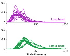
      Data reported in Figure 5 should be quantified (cell numbers, how many brains analyzed). 

      Thank you for this comment. We would like to clarify that the primary purpose of Figure 5 (and Figure 5 supplement 1) is to provide an initial qualitative overview of the different MNP subsets present in the adult brain, using the currently available transgenic and immunohistochemical tools. These descriptive analyses were instrumental in identifying the most reliable combination, namely the Tg(p2ry12:p2ry12GFP; mpeg1.1:mCherry) double transgenic line in conjunction with L-plastin immunostaining, to distinguish microglia from other parenchymal MNPs. Quantitative analyses using this optimized strategy are presented in Figure 7 (Figure 7 supplement 1), where we systematically enumerate the different MNPs. We therefore believe that performing additional quantification in Figure 5 would be redundant with the more robust data already shown in Figure 7. As requested, we have now included in the Figure 5 legend that images are representative of brain tissue sections from 2-3 fish. 

      The title mentions an "atlas", but there is no searchable database or website associated with the paper. Please provide one.

      We agree and fully support the importance of data accessibility. To facilitate use of our dataset by the scientific community, we have developed a user-friendly, searchable web interface that allows users to explore gene expression pacerns within our dataset. This website is available at https://scrna-analysis zebrafish.shinyapps.io/scatlas/

      This information has now been included in the “Data availability statement” section of the manuscript.  

      Reviewer #1 (Recommendations For The Authors): 

      Specific comments: 

      The authors should discuss another recent report demonstrating DCs in the zebrafish brain, which also developed independently of Csf1ra, and compare the two datasets (Zhou et al. Cell reports, 2023). 

      Thank you for this suggestion. Please refer to our response in the major comments section, where we address this point in detail.

      Within macrophages, the authors identified 5 clusters including 4 microglia clusters and 1 MF cluster (Figure 4). Does the laUer relate to 'BAMs' and express markers previously described in murine BAMs, including Lyve1, CD206, etc.? Or to monocytes? By flow cytometry, monocytes were detected (Figure 1B), but not by scRNA-seq.  

      You have raised an important point here. As described in lines 197-202 (“results” section), the cells in the MF cluster exhibit a macrophage identity, based on their expression of classical macrophage markers such as marco, mfap4 or csf1ra. However, we were unable to confidently annotate this cluster more specifically. We also considered whether this population might resemble mammalian BAMs or monocytes, cell types that, to our knowledge, have not yet been clearly identified in zebrafish. However, orthologous markers typically associated with murine BAMs were not detected (lyve1) or not specifically enriched (mrc1a/mrc1b) in the MF cluster (see below). Based on these findings, we can only cautiously propose that this cluster may represent blood-derived macrophages and / or monocytes. 

      To further address your suggestion, we performed a cell type enrichment analysis using the marker genes of the MF cluster, following the same strategy as for the microglia and DC-like clusters presented in Figure 4 supplement 2 C,D. This analysis revealed significant for “monocytes” and “macrophages”, further supporting a general monocytic/macrophage identity (see below). At present, further characterization of this cluster is limited by the lack of zebrafish-specific antibodies and the restricted palette of fluorescent reporter lines that distinguish among MNP subsets. We anticipate that future studies, including the development of new transgenic lines guided by our dataset, will allow for a more precise analysis of this distinct population. 

      Author response image 1.

      Do all 4 DC clusters identified by scRNA-seq represent cDC1s? or are there also cDC2s, and cDC3s present?  

      In our analyses, the four dendritic cell clusters identified by scRNA-seq (DC1-DC4) exhibit transcriptional profiles consistent with a conventional type 1 dendritic cell (cDC1) identity. These clusters uniformly express hallmark cDC1-associated genes, while lacking expression of markers typically associated with mammalian cDC2 or plasmacytoid dendritic cells (pDCs). For instance, irf4, a key transcription factor required for cDC2 development, is not detected in our dataset. Similarly, we do not observe expression of genes characteristic of pDCs. 

      That said, the absence of cDC2 or pDC-like signatures in our dataset does not rule out the presence of these populations in zebrafish.  

      While they show that DC-like cells did not express Csf1rb (Figure 4D) or other macrophage/microglia genes, DC-like cells were affected in the Csf1rb mutants and in double mutants, demonstrating that their development depends on Csf1rb signaling, as known for macrophages but not DCs. Can the authors discuss this in more detail with regard to DC differentiation/precursors? 

      Thank you for pointing this out. As previously demonstrated, CSF1R signaling in zebrafish is more complex than in mammals, due to the presence of two paralogs, csf1ra and csf1rb, which exhibit partially non-overlapping functions (Ferrero et al., 2021). We and others have shown that csf1rb signaling is implicated in the regulation of definitive hematopoiesis, particularly in the regulation of hematopoietic stem cell (HSC)-derived myelopoiesis. Although the developmental origin of zebrafish brain DC-like cells remains uncharacterized, their reduced numbers in the csf1rb mutant, despite their lack of csf1rb expression, supports the current model in which csf1rb acts at the progenitor level, promoting myeloid lineage commitment. According to this, csf1rb disruption affects the differentiation of multiple myeloid subsets, which likely include DC-like cells. We have developed this point in the discussion section (lines 502506).  

      Do the DCs express Csf1ra? 

      Csf1ra transcripts are not found in DCs in our dataset. As shown below, csf1ra expression is restricted to the microglia and macrophage clusters. These observations are in line with those made by Zhou et al., 2023.

      Author response image 2.

      Fig. 5, the number of brains analyzed should be added, and also quantifications of cell numbers included. It is mentioned (line 260) that P2ry12GFP+mpeg1mCherry+ microglia are abundant across brain regions while P2ry12GFP- mpeg1mCherry+ cells particularly localize in the ventral part of the posterior brain parenchyma. It would be nice if images of the different brain regions were provided. 

      Regarding the quantification, we refer to our response in the major comments section, where we explain that detailed quantification of microglia and other MNP subsets is provided in Figure 7, using a more refined strategy for distinguishing cell types.

      As requested, we have now included representative sections from the forebrain, midbrain and hindbrain of adult Tg(mhc2dab:GFP; cd45:DsRed) fish. These images illustrate the spatial distribution of DC-like cells across brain regions. Notably, DC-like cells are most abundant in the ventral areas of the midbrain and hindbrain, and are also present in the posterior telencephalon, particularly concentrated in the region of the commissura anterior. This regional annotation is based on the zebrafish brain atlas by Wullimann et al., 1996 (Neuroanatomy of the zebrafish brain, https://doi.org/10.1007/978-3-0348-8979-7).

      These additional images have been included in Figure 5 Supplement 1 (A-E).

      It is sometimes not evident whether the Pr2y12- cells included DC-like cells and macrophages, which should be discussed. 

      Thank you for bringing this to our attention. Upon review, we agree this point required clearer explanation throughout the text, particularly beginning with the description of putative DC-like cells in Figure 5. We have now revised the manuscript to improve clarity and becer guide readers through the phenotypic identification of DC-like cells using the Tg(p2ry12:p2ry12-GFP;mpeg1:mCherry) line. Specifically, we have modified the titles in the results section from page 5 to page 9, so that readers can more easily follow the step-by-step approach we used to distinguish DC-like cells from microglia. 

      To directly address your comment: the p2ry12<sup>-</sup>; mpeg1<sup>+</sup> fraction may, in theory, include not only DC-like cells but also other macrophage subsets and B cells, as B cells have been shown to express mpeg1 in zebrafish (Ferrero et al., 2020; Moyse et al., 2020). Nevertheless, our data strongly indicate that within the brain parenchyma, DC-like cells represent the predominant component of this population. This conclusion is supported by the pronounced reduction of p2ry12<sup>-</sup>; mpeg1<sup>+</sup> cells in brain sections from ba43 mutants, in which DC development is impaired. 

      We have revised the text accordingly to clarify this point in the results section of the manuscript (line 355).

      For example, the DC-like cell population in Figure 6C appears to include two populations of cells. Thus, it is unclear whether the sorted mhc2dab:GFP+;CD45:DsRedhi population for bulk-seq also contains the MF population identified in Fig. 2. 

      Thank you for this thoughtful observation. During the course of this study, we indeed considered how best to isolate non-microglial macrophages in order to specifically recover the MF population identified in our scRNA-seq analysis. However, with the current repertoire of fluorescent transgenic zebrafish lines, it remains technically challenging to selectively isolate non-microglial macrophages from the adult brain. As a result, the mhc2dab:GFP⁺; cd45:DsRedhi sorted population used for bulk RNA-seq may indeed include a mixture of DC-like and other mononuclear phagocytes, potentially the MF population. In contrast, our data demonstrate that the Tg(p2ry12:p2ry12-GFP) line provides a more selective tool for isolating microglia, minimizing contamination from other mononuclear phagocyte subsets.

      In Figure 7, a reduction of GFP-mpeg+ cells can be seen in baf3 mutants. Could the remaining cells be the (non-microglia) macrophages? Or in Figure 8, could the remaining P2ry12GFP-Lcp1+ cells in Irf8 mutants be macrophages? 

      Indeed, we believe it is likely that the remaining mpeg1<sup>+</sup> cells observed in ba43 mutants include non-microglial macrophages and/or B cells, as we and others previously showed that zebrafish B cells express mpeg1.1 transcripts and are labeled in the mpeg1.1 reporters (Ferrero et al., 2020). This interpretation is further supported by the observation that the reduction in mepg1+ cells is more pronounced in brain sections than in flow cytometry samples, where non-parenchymal mpeg+ cells, such as peripheral macrophages or B cells, are likely enriched. To explore this possibility, we attempted to assess the expression of MF- and B cell-specific markers in the remaining mpeg1+ population isolated from ba43 mutants. However, due to the very low numbers of cells recovered per animal, we were limited to analyzing only a few markers. Despite multiple attempts, qPCR analyses proved unconclusive, likely due to low transcript abundance. We thank you for your understanding of the technical limitations that currently prevent a more definitive characterization of these remaining cells.  

      Regarding the irf8 mutants (Figure 8), irf8 is a well-established master regulator of mononuclear phagocyte development. In mice, deficiency results in developmental defects and functional impairments across multiple myeloid lineages, including microglia, which exhibit reduced density (Kierdorf et al., 2013) and an immature phenotype (Vanhove and al., 2019)). Similarly, in zebrafish, irf8 mutants show abnormal macrophage development, with an accumulation of immature and apoptotic cells during embryonic and larval stages (Shiau et al., 2014). Based on these findings, it is plausible that the residual p2ry12:GFP<sup>-</sup> Lcp1<sup>+</sup> cells observed in the irf8 mutant brains represent immature or arrested mononuclear phagocytes, possibly including both microglia and DC-like cells. This is supported by their distinct morphology and specific localization along the ventricle borders. However, as previously noted, our current tools do not permit to conclusively identify these cells.

      Reviewer #2 (Recommendations For The Authors): 

      A few sentences are not easy   to understand for a "non zebrafish specialist". 

      (1) Page 3 line 111 The sentence "Interestingly, analyses of brain cell suspensions from double transgenics showed p2ry12:GFP+ microglia accounted for half of cd45:DsRed+ cells (50.9 % {plus minus} 2.9; n=4) (Figure 1D,E). Considering that mpeg1:GFP+ cells comprised ~75% of all leukocytes, these results indicated that approximately 25% of brain mononuclear phagocytes do not express the microglial p2ry12:GFP+ transgene." is not clear. This point is significant and deserves a more detailed explanation. 

      We apologize for the lack of clarity in this section. The quantification presented in Figure 1 refers specifically to cd45:Dsred<sup>+</sup> leukocytes, meaning that the reported percentages of p2ry12:GFP<sup>+</sup> and mpeg1:GFP<sup>+</sup> cells are calculated relative to the total cd45+ population (defined as 100%). Specifically, we observed that approximately 51% of all cd45+ cells were p2r12:GFP<sup>+</sup> microglia, while around ti5% were mpeg1:GFP<sup>+</sup>. From these values, we infer that about 25% of mpeg1:GFP<sup>+</sup> leukocytes do not express the p2ry12:GFP transgene and therefore likely represent non-microglial mononuclear phagocytes. We agree that this distinction is important and have revised the text accordingly to clarify the interpretation for readers who may be less familiar with zebrafish transgenic lines or gating strategies. See page 3, lines 107 117.

      (2) Line 522; Like human and mouse ILC2s, "these cells do not express the T cell receptor cd4-1" is confusing (T cell receptor should be reserved to the ag specific TCR). Also, was TCR isotypes expression analyzed (and how was genome annotation used in this case ?) 

      Thank you for this insightful comment.  We agree that the term “T cell receptor” should be used specifically to refer to antigen-specific TCRs, and we have revised the discussion accordingly to avoid any confusion. Regarding your question on the analysis of TCR isotype expression and the use of genome annotation: due to technical limitations, we did not pursue TCR isotype-level analysis in this study. Instead, we relied on established markers such as cd4-1 and cd8a to distinguish T cell populations, acknowledging that cd4-1 is not expressed by ILC2-like cells in our dataset. We have clarified these points in the relevant sections of the manuscript (see lines 168 and 535)

      The analysis of single-cell data might be more detailed, with more explanation about possible doublet identification and normalization procedures. 

      Thank you for highlighting the need for additional clarity regarding our scRNA-seq analysis.

      As noted in the Seurat tutorial, “cell doublets or multiplets often exhibit abnormally high gene count” (https://sa7jalab.org/seurat/archive/v3.0/pbmc3k_tutorial). To evaluate this, we performed a dedicated doublet detection analysis using the scDblFinder R package (https://rdrr.io/bioc/scDblFinder/f/vigneces/2_scDblFinder.Rmd). Our results indicated that the proportion of predicted doublets is low (see Figure below), and when present, these doublets are distributed among the different clusters. This contrasts with the typical clustering of doublets into discrete groups and indicates that our single-cell sequencing workflow was sufficiently robust to predominantly capture singlets.

      Regarding normalization, we have clarified this in the manuscript. Briefly, single-cell data were normalized using Seurat’s SCTransform method with the following custom parameters: “variable.features.n=4000 and return.only.var.genes=F”. These settings are now clearly described to ensure reproducibility.

      Author response image 3.

      Reviewer #3 (Recommenda,ons For The Authors):

      Major issues

      Though baf3 mutants were generated the manuscript will greatly benefit from in situ labeling by RNAscope or the generation of transgenic reporters to conclusively localize this dendritic cell population and address any potential contamination issues. 

      We thank you for this constructive suggestion. We agree that in situ labeling approaches such as RNAscope would offer valuable complementary insights. In our current study, however, we already provide detailed spatial information on DC-like cells, and we demonstrated their lineage identity through the use of our newly generated batf3 mutant line. 

      To address concerns regarding potential contamination, we have carefully analyzed more than two dozens adult brains to date and consistently observed abundant DC-like cells within the brain parenchyma, exhibiting a reproducible and specific spatial distribution, as described in the manuscript. This consistent localization across multiple samples strongly supports the genuine presence of these cells in the brain rather than artifactual contamination.

      While the generation of DC-like specific transgenic lines is indeed a promising direction (and such efforts are currently underway in our group) we note that creating and validating these lines is time-consuming and falls beyond the scope of the present study. Importantly, although these additional tools will be valuable for future functional investigations, we believe they would not impact the main conclusions or core message of our current work. 

      The morphological characterization of CD45:DsRed+ macrophages stained with May-Grunwald-Giemsa has been previously reported in the paper, "Characterization of the mononuclear phagocyte system in the zebrafish" Wittamer et al., 2011."Morphologic analyses revealed that the majority of cells exhibited the characteristics of monocytes/macrophages namely low nuclear to cytoplasm ratios and a high number of cytoplasmic vacuoles (Figure 3B). 

      We thank you for pointing out the reference to Wittamer et al., 2011. In that study, we indeed provided the first morphological characterization of mononuclear phagocytes (MNPs) in various adult zebrafish organs using the cd45:DsRed line in combination with the mhc2dab:GFP reporter. The focus was primarily on MNPs across peripheral tissues. In the current study, our aim is broader: we investigate the full diversity of brain immune cells, using cd45 as a general marker for leukocytes. As part of this comprehensive characterization, we applied MGG staining, a widely accepted cytological technique, to gain morphological insight into the sorted CD45:DsRed+ population. This method remains a valuable and rapid approach to visually assess cell type heterogeneity, especially when evaluating samples where multiple immune cell lineages may be present. 

      While there is some overlap with the methodology used in Wittamer et al., the context, scope, and tissue examined differ substantially. Thus, the inclusion of MGG staining in this study serves to complement our broader transcriptomic analyses by providing supporting morphological evidence specific to brain-resident immune cells.

      We have now clarified this distinction in the revised manuscript to better differentiate the current work from our previous findings (see line 85).

      Figure 5 data should be quantified.

      Please refer to our response in the major comments section, where we address this question in detail.

      Figure 7- Figure Supplement 1. J, K has no CD45:DsRed positive cells in baf3 mutants, which is counterintuitive because CD45:DsRed should capture all hematopoietic cells and is not specific to dendritic cells. 

      It is correct that cd45 is a general leukocyte marker, labeling all immune cells, including dendritic cells. In this Figure, we used the Tg(cd45:DsRed) transgenic line to visualize the phenotype because it offers an alternative to IHC, with the advantage of strong endogenous fluorescence and easier screening of vibratome sections. However, this technique has limitations: due to fixation, only cells with high fluorescence (e.g. cd45<sup>high</sup>dendritic cells) are captured, while those with medium/low expression (e.g. cd45<sup>low</sup> microglia) are often not visible. This explains why fewer cells are observed in both wild-type and ba43 mutant brains (Figure 5 KN, Figure 7 – supplement 1 JK). While this approach is quicker and allows for thicker sections, IHC remains the preferred method for the rest of the analyses, including the use of additional markers to identify all relevant cell populations. 

      Thank you for bringing this point of confusion to our attention. To improve clarity, we have amended the text in the relevant sections (see lines 704-706, and legend of Figure 7 Supplement 1)

      Minor issues: 

      The terms in the title, "A single-cell transcriptomic atlas..." are used. What is meant by "atlas"? A searchable database or website is not provided. 

      Please refer to our response in the major comments section, where we explain that we have made our dataset accessible through a searchable web interface (https://scrna-analysiszebrafish.shinyapps.io/scatlas/) which is now referenced in the Data Availability Statement.

      This reviewer considers that it is offensive to use terminology such as "poorly characterized" in reference to others' work. 

      Thank you for pointing this out. We understand the concern and have revised the wording to ensure it remains respectful and neutral when referring to previous work. The changes are reflected in lines 20 and 49.

      The introduction of this manuscript should consider restructuring and editing. Example: Lines 51-5ti introduce the importance of immune cells in zebrafish regeneration studies. However, this study does not investigate such processes. Additionally, the authors focus on the concept of immune heterogeneity in the brain throughout the text however, these studies have been conducted previously by others (Silva et al., 2021) at single-cell level. 

      The novelty of this manuscript is the identification of "dendritic-like cells" and yet the introduction and text are limited to 68-ti1 lines. The introduction would benefit by introducing this cell type "dendritic-like cells" and differences between vertebrates. 

      Thank you for these valuable comments. In response, we have revised the introduction to better align with the focus of the study (see edited text in page 2). We now emphasize that, while macrophages have been extensively studied in zebrafish, dendritic cells remain much less well characterized in this model.  Also, while we acknowledge that Silva et al. addressed aspects of immune heterogeneity in the zebrafish brain, their study primarily focused on mononuclear phagocytes. In contrast, our work provides a broader and more detailed characterization of the brain immune landscape, integrating transcriptomic data with multiple fluorescent reporter lines and hematopoietic mutants to strengthen cell identity assignments. Importantly, we note that Silva et al. classified DC-like cells within the microglial compartment, whereas our findings support that these cells represent a distinct population. While our data challenge this specific aspect of their conclusions, we believe both studies offer complementary insights that collectively advance our understanding of zebrafish brain immunity. 

      Though Figure 6 is a great conformation of scRNA sequencing, it seems redundant and should be supplemental data.

      We respectfully disagree with the reviewer’s suggestion. We believe that presenting the data in Figure 6 as the main figure enhances its visibility and impact, particularly highlighting the distinction between microglia and DC-like cells, an aspect we consider highly valuable information for the zebrafish research community. This is especially important given that our conclusions challenge two previous independent reports, further underscoring the relevance of these findings to the field.

    1. eLife Assessment

      This study presents SegPore, a valuable new method for processing direct RNA nanopore sequencing data, which improves the segmentation of raw signals into individual bases and boosts the accuracy of modified base detection. The evidence presented to benchmark SegPore is solid, and the authors provide a fully documented implementation of the method. SegPore will be of particular interest to researchers studying RNA modifications.

    2. Reviewer #1 (Public review):

      Summary:

      In this manuscript, the authors describe a new computational method (SegPore), which segments the raw signal from nanopore direct RNA-Seq data to improve the identification of RNA modifications. In addition to signal segmentation, SegPore includes a Gaussian Mixture Model approach to differentiate modified and unmodified bases. SegPore uses Nanopolish to define a first segmentation, which is then refined into base and transition blocks. SegPore also includes a modification prediction model that is included in the output. The authors evaluate the segmentation in comparison to Nanopolish and Tombo (RNA002) as well as f5c and Uncalled 4 (RNA004), and they evaluate the impact on m6A RNA modification detection using data with known m6A sites. In comparison to existing methods, SegPore appears to improve the ability to detect m6A, suggesting that this approach could be used to improve the analysis of direct RNA-Seq data.

      Strengths:

      SegPore address an important problem (signal data segmentation). By refining the signal into transition and base blocks, noise appears to be reduced, leading to improved m6A identification at the site level as well as for single read predictions. The authors provide a fully documented implementation, including a GPU version that reduces run time. The authors provide a detailed methods description, and the approach to refine segments appears to be new.

      Weaknesses:

      The authors show that SegPore reduces noise compared to other methods, however the improvement in accuracy appears to be relatively small for the task of identifying m6A. To run SegPore, the GPU version is essential, which could limit the application of this method in practice.

    3. Reviewer #2 (Public review):

      Summary:

      The work seeks to improve detection of RNA m6A modifications using Nanopore sequencing through improvements in raw data analysis. These improvements are said to be in the segmentation of the raw data, although the work appears to position the alignment of raw data to the reference sequence and some further processing as part of the segmentation, and result statistics are mostly shown on the 'data-assigned-to-kmer' level.<br /> As such, the title, abstract and introduction stating the improvement of just the 'segmentation' does not seem to match the work the manuscript actually presents, as the wording seems a bit too limited for the work involved.<br /> The work itself shows minor improvements in m6Anet when replacing Nanopolish' eventalign with this new approach, but clear improvements in the distributions of data assigned per kmer. However, these assignments were improved well enough to enable m6A calling from them directly, both at site-level and at read-level.

      A large part of the improvements shown appear to stem from the addition of extra, non-base/kmer specific, states in the segmentation/assignment of the raw data, removing a significant portion of what can be considered technical noise for further analysis. Previous methods enforced assignment of (almost) all raw data, forcing a technically optimal alignment that may lead to suboptimal results in downstream processing as datapoints could be assigned to neighbouring kmers instead, while random noise that is assigned to the correct kmer may also lead to errors in modification detection.

      For an optimal alignment between the raw signal and the reference sequence, this approach may yield improvements for downstream processing using other tools.<br /> Additionally, the GMM used for calling the m6A modifications provides a useful, simple and understandable logic to explain the reason a modification was called, as opposed to the black models that are nowadays often employed for these types of tasks.

      Weaknesses:

      The manuscript suggests the eventalign results are improved compared to Nanopolish. While this is believably shown to be true (Table 1), the effect on the use case presented, downstream differentiation between modified and unmodified status on a base/kmer, is likely limited for during downstream modification calling the noisy distributions are often 'good enough'. E.g. Nanopolish uses the main segmentation+alignment for a first alignment and follows up with a form of targeted local realignment/HMM test for modification calling (and for training too), decreasing the need for the near-perfect segmentation+alignment this work attempts to provide. Any tool applying a similar strategy probably largely negates the problems this manuscript aims to improve upon. Should a use-case come up where this downstream optimisation is not an option, SegPore might provide the necessary improvements in raw data alignment.

      Appraisal:

      The authors have shown their methods ability to identify noise in the raw signal and remove their values from the segmentation and alignment, reducing its influences for further analyses. Figures directly comparing the values per kmer do show a visibly improved assignment of raw data per kmer. As a replacement for Nanopolish' eventalign it seems to have a rather limited, but improved effect, on m6Anet results. At the single read level modification modification calling this work does appear to improve upon CHEUI.

      Impact:

      With the current developments for Nanopore based modification calling largely focusing on Artificial Intelligence, Neural Networks and the likes, improvements made in interpretable approaches provide an important alternative that enables deeper understanding of the data rather than providing a tool that plainly answers the question of wether a base is modified or not, without further explanation. The work presented is best viewed in context of a workflow where one aims to get an optimal alignment between raw signal data and the reference base sequence for further processing. For example, as presented, as a possible replacement for Nanopolish' eventalign. Here it might enable data exploration and downstream modification calling without the need for local realignments or other approaches that re-consider the distribution of raw data around the target motif, such as a 'local' Hidden Markov Model or Neural Networks. These possibilities are useful for a deeper understanding of the data and further tool development for modification detection works beyond m6A calling.

    4. Reviewer #3 (Public review):

      Summary:

      Nucleotide modifications are important regulators of biological function, however, until recently, their study has been limited by the availability of appropriate analytical methods. Oxford Nanopore direct RNA sequencing preserves nucleotide modifications, permitting their study, however many different nucleotide modifications lack an available base-caller to accurately identify them. Furthermore, existing tools are computationally intensive, and their results can be difficult to interpret.

      Cheng et al. present SegPore, a method designed to improve the segmentation of direct RNA sequencing data and boost the accuracy of modified base detection.

      Strengths:

      This method is well described and has been benchmarked against a range of publicly available base callers that have been designed to detect modified nucleotides.

      Weaknesses:

      However, the manuscript has a significant drawback in its current version. The most recent nanopore RNA base callers can distinguish between different ribonucleotide modifications, however, SegPore has not been benchmarked against these models.

      The manuscript would be strengthened by benchmarking against the rna004_130bps_hac@v5.1.0 and rna004_130bps_sup@v5.1.0 dorado models, which are reported to detect m5C, m6A_DRACH, inosine_m6A and PseU.

      A clear demonstration that SegPore also outperforms the newer RNA base caller models will confirm the utility of this method.

    5. Author response:

      The following is the authors’ response to the original reviews

      We thank all the reviewers for their constructive comments. We have carefully considered your feedback and revised the manuscript accordingly. The major concern raised was the applicability of SegPore to the RNA004 dataset. To address this, we compared SegPore with f5c and Uncalled4 on RNA004, and found that SegPore demonstrated improved performance, as shown in Table 2 of the revised manuscript.
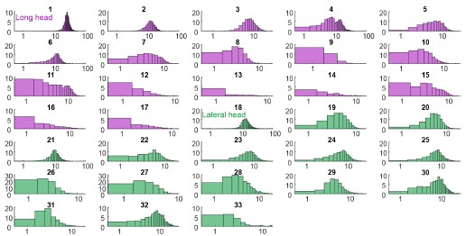
      Following the reviewers’ recommendations, we updated Figures 3 and 4. Additionally, we added one table and three supplementary figures to the revised manuscript:

      · Table 2: Segmentation benchmark on RNA004 data

      · Supplementary Figure S4: RNA translocation hypothesis illustrated on RNA004 data

      · Supplementary Figure S5: Illustration of Nanopolish raw signal segmentation with eventalign results

      · Supplementary Figure S6: Running time of SegPore on datasets of varying sizes

      Below, we provide a point-by-point response to your comments.

      Reviewer #1 (Public review):

      Summary:

      In this manuscript, the authors describe a new computational method (SegPore), which segments the raw signal from nanopore-direct RNA-Seq data to improve the identification of RNA modifications. In addition to signal segmentation, SegPore includes a Gaussian Mixture Model approach to differentiate modified and unmodified bases. SegPore uses Nanopolish to define a first segmentation, which is then refined into base and transition blocks. SegPore also includes a modification prediction model that is included in the output. The authors evaluate the segmentation in comparison to Nanopolish and Tombo, and they evaluate the impact on m6A RNA modification detection using data with known m6A sites. In comparison to existing methods, SegPore appears to improve the ability to detect m6A, suggesting that this approach could be used to improve the analysis of direct RNA-Seq data.

      Strengths:

      SegPore addresses an important problem (signal data segmentation). By refining the signal into transition and base blocks, noise appears to be reduced, leading to improved m6A identification at the site level as well as for single-read predictions. The authors provide a fully documented implementation, including a GPU version that reduces run time. The authors provide a detailed methods description, and the approach to refine segments appears to be new.

      Weaknesses:

      In addition to Nanopolish and Tombo, f5c and Uncalled4 can also be used for segmentation, however, the comparison to these methods is not shown.

      The method was only applied to data from the RNA002 direct RNA-Sequencing version, which is not available anymore, currently, it remains unclear if the methods still work on RNA004.

      Thank you for your comments.

      To clarify the background, there are two kits for Nanopore direct RNA sequencing: RNA002 (the older version) and RNA004 (the newer version). Oxford Nanopore Technologies (ONT) introduced the RNA004 kit in early 2024 and has since discontinued RNA002. Consequently, most public datasets are based on RNA002, with relatively few available for RNA004 (as of 30 June 2025).

      Nanopolish and Tombo were developed for raw signal segmentation and alignment using RNA002 data, whereas f5c and Uncalled4are the only two software supporting RNA004 data.  Since the development of SegPore began in January 2022, we initially focused on RNA002 due to its data availability. Accordingly, our original comparisons were made against Nanopolish and Tombo using RNA002 data.

      We have now updated SegPore to support RNA004 and compared its performance against f5c and Uncalled4 on three public RNA004 datasets.

      As shown in Table 2 of the revised manuscript, SegPore outperforms both f5c and Uncalled4 in raw signal segmentation. Moreover, the jiggling translocation hypothesis underlying SegPore is further supported, as shown in Supplementary Figure S4.

      The overall improvement in accuracy appears to be relatively small.

      Thank you for the comment.

      We understand that the improvements shown in Tables 1 and 2 may appear modest at first glance due to the small differences in the reported standard deviation (std) values. However, even small absolute changes in std can correspond to substantial relative reductions in noise, especially when the total variance is low.

      To better quantify the improvement, we assume that approximately 20% of the std for Nanopolish, Tombo, f5c, and Uncalled4 arises from noise. Using this assumption, we calculate the relative noise reduction rate of SegPore as follows:

      Noise reduction rate = (baseline std − SegPore std) / (0.2 × baseline std) ​​

      Based on this formula, the average noise reduction rates across all datasets are:

      - SegPore vs Nanopolish: 49.52%

      - SegPore vs Tombo: 167.80%

      - SegPore vs f5c: 9.44%

      - SegPore vs Uncalled4: 136.70%

      These results demonstrate that SegPore can reduce the noise level by at least 9% given a noise level of 20%, which we consider a meaningful improvement for downstream tasks, such as base modification detection and signal interpretation. The high noise reduction rates observed in Tombo and Uncalled4 (over 100%) suggest that their actual noise proportion may be higher than our 20% assumption.

      We acknowledge that this 20% noise level assumption is an approximation. Our intention is to illustrate that SegPore provides measurable improvements in relative terms, even when absolute differences appear small.

      The run time and resources that are required to run SegPore are not shown, however, it appears that the GPU version is essential, which could limit the application of this method in practice.

      Thank you for your comment.

      Detailed instructions for running SegPore are provided in github (https://github.com/guangzhaocs/SegPore). Regarding computational resources, SegPore currently requires one CPU core and one Nvidia GPU to perform the segmentation task efficiently.

      We present SegPore’s runtime for typical datasets in Supplementary Figure S6 in the revised manuscript.  For a typical 1 GB fast5 file, the segmentation takes approximately 9.4 hours using a single NVIDIA DGX‑1 V100 GPU and one CPU core.

      Currently, GPU acceleration is essential to achieve practical runtimes with SegPore. We acknowledge that this requirement may limit accessibility in some environments. To address this, we are actively working on a full C++ implementation of SegPore that will support CPU-only execution. While development is ongoing, we aim to release this version in a future update.

      Reviewer #2 (Public review):

      Summary:

      The work seeks to improve the detection of RNA m6A modifications using Nanopore sequencing through improvements in raw data analysis. These improvements are said to be in the segmentation of the raw data, although the work appears to position the alignment of raw data to the reference sequence and some further processing as part of the segmentation, and result statistics are mostly shown on the 'data-assigned-to-kmer' level.

      As such, the title, abstract, and introduction stating the improvement of just the 'segmentation' does not seem to match the work the manuscript actually presents, as the wording seems a bit too limited for the work involved.

      The work itself shows minor improvements in m6Anet when replacing Nanopolish eventalign with this new approach, but clear improvements in the distributions of data assigned per kmer. However, these assignments were improved well enough to enable m6A calling from them directly, both at site-level and at read-level.

      Strengths:

      A large part of the improvements shown appear to stem from the addition of extra, non-base/kmer specific, states in the segmentation/assignment of the raw data, removing a significant portion of what can be considered technical noise for further analysis. Previous methods enforced the assignment of all raw data, forcing a technically optimal alignment that may lead to suboptimal results in downstream processing as data points could be assigned to neighbouring kmers instead, while random noise that is assigned to the correct kmer may also lead to errors in modification detection.

      For an optimal alignment between the raw signal and the reference sequence, this approach may yield improvements for downstream processing using other tools.<br /> Additionally, the GMM used for calling the m6A modifications provides a useful, simple, and understandable logic to explain the reason a modification was called, as opposed to the black models that are nowadays often employed for these types of tasks.

      Weaknesses:

      The work seems limited in applicability largely due to the focus on the R9's 5mer models. The R9 flow cells are phased out and not available to buy anymore. Instead, the R10 flow cells with larger kmer models are the new standard, and the applicability of this tool on such data is not shown. We may expect similar behaviour from the raw sequencing data where the noise and transition states are still helpful, but the increased kmer size introduces a large amount of extra computing required to process data and without knowledge of how SegPore scales, it is difficult to tell how useful it will really be. The discussion suggests possible accuracy improvements moving to 7mers or 9mers, but no reason why this was not attempted.

      Thank you for pointing out this important limitation. Please refer to our response to Point 1 of Reviewer 1 for SegPore’s performance on RNA004 data. Notably, the jiggling behavior is also observed in RNA004 data, and SegPore achieves better performance than both f5c and Uncalled4.

      The increased k-mer size in RNA004 affects only the training phase of SegPore (refer to Supplementary Note 1, Figure 5 for details on the training and testing phases). Once the baseline means and standard deviations for each k-mer are established, applying SegPore to RNA004 data proceeds similarly to RNA002. This is because each k-mer in the reference sequence has, at most, two states (modified and unmodified). While the larger k-mer size increases the size of the parameter table, it does not increase the computational complexity during segmentation. Although estimating the initial k-mer parameter table requires significant time and effort on our part, it does not affect the runtime for end users applying SegPore to RNA004 data.

      Extending SegPore from 5-mers to 7-mers or 9-mers for RNA002 data would require substantial effort to retrain the model and generate sufficient training data. Additionally, such an extension would make SegPore’s output incompatible with widely used upstream and downstream tools such as Nanopolish and m6Anet, complicating integration and comparison. For these reasons, we leave this extension for future work.

      The manuscript suggests the eventalign results are improved compared to Nanopolish. While this is believably shown to be true (Table 1), the effect on the use case presented, downstream differentiation between modified and unmodified status on a base/kmer, is likely limited as during actual modification calling the noisy distributions are usually 'good enough', and not skewed significantly in one direction to really affect the results too terribly.

      Thank you for your comment. While current state-of-the-art (SOTA) methods perform well on benchmark datasets, there remains significant room for improvement. Most SOTA evaluations are based on limited datasets, primarily covering DRACH motifs in human and mouse transcriptomes. However, m6A modifications can also occur in non-DRACH motifs, where current models may underperform. Additionally, other RNA modifications—such as pseudouridine, inosine, and m5C—are less studied, and their detection may benefit from improved signal modeling.

      We would also like to emphasize that raw signal segmentation and RNA modification detection are distinct tasks. SegPore focuses on the former, providing a cleaner, more interpretable signal that can serve as a foundation for downstream tasks. Improved segmentation may facilitate the development of more accurate RNA modification detection algorithms by the community.

      Scientific progress often builds incrementally through targeted improvements to foundational components. We believe that enhancing signal segmentation, as SegPore does, contributes meaningfully to the broader field—the full impact will become clearer as the tool is adopted into more complex workflows.

      Furthermore, looking at alternative approaches where this kind of segmentation could be applied, Nanopolish uses the main segmentation+alignment for a first alignment and follows up with a form of targeted local realignment/HMM test for modification calling (and for training too), decreasing the need for the near-perfect segmentation+alignment this work attempts to provide. Any tool applying a similar strategy probably largely negates the problems this manuscript aims to improve upon.

      We thank the reviewer for this insightful comment.

      To clarify, Nanopolish provides three independent commands: polya, eventalign, and call-methylation.

      - The polya command identifies the adapter, poly(A) tail, and transcript region in the raw signal.

      - The eventalign command aligns the raw signal to a reference sequence, assigning a signal segment to individual k-mers in the reference.

      - The call-methylation command detects methylated bases from DNA sequencing data.

      The eventalign command corresponds to “the main segmentation+alignment for a first alignment,” while call-methylation corresponds to “a form of targeted local realignment/HMM test for modification calling,” as mentioned in the reviewer’s comment. SegPore’s segmentation is similar in purpose to Nanopolish’s eventalign, while its RNA modification estimation component is similar in concept to Nanopolish’s call-methylation.

      We agree the general idea may appear similar, but the implementations are entirely different. Importantly, Nanopolish’s call-methylation is designed for DNA sequencing data, and its models are not trained to recognize RNA modifications. This means they address distinct research questions and cannot be directly compared on the same RNA modification estimation task. However, it is valid to compare them on the segmentation task, where SegPore exhibits better performance (Table 1).

      We infer the reviewer may suggest that because m6Anet is a deep neural network capable of learning from noisy input, the benefit of more accurate segmentation (such as that provided by SegPore) might be limited. This concern may arise from the limited improvement of SegPore+m6Anet over Nanopolish+m6Anet in bulk analysis (Figure 3). Several factors may contribute to this observation:

      (i) For reads aligned to the same gene in the in vivo data, alignment may be inaccurate due to pseudogenes or transcript isoforms.

      (ii) The in vivo benchmark data are inherently more complex than in vitro datasets and may contain additional modifications (e.g., m5C, m7G), which can confound m6A calling by altering the signal baselines of k-mers.

      (iii) m6Anet is trained on events produced by Nanopolish and may not be optimal for SegPore-derived events.

      (iv) The benchmark dataset lacks a modification-free (IVT) control sample, making it difficult to establish a true baseline for each k-mer.

      In the IVT data (Figure 4), SegPore shows a clear improvement in single-molecule m6A identification, with a 3~4% gain in both ROC-AUC and PR-AUC. This demonstrates SegPore’s practical benefit for applications requiring higher sensitivity at the molecule level.

      As noted earlier, SegPore’s contribution lies in denoising and improving the accuracy of raw signal segmentation, which is a foundational step in many downstream analyses. While it may not yet lead to a dramatic improvement in all applications, it already provides valuable insights into the sequencing process (e.g., cleaner signal profiles in Figure 4) and enables measurable gains in modification detection at the single-read level. We believe SegPore lays the groundwork for developing more accurate and generalizable RNA modification detection tools beyond m6A.

      We have also added the following sentence in the discussion to highlight SegPore’s limited performance in bulk analysis:

      “The limited improvement of SegPore combined with m6Anet over Nanopolish+m6Anet in bulk in vivo analysis (Figure 3) may be explained by several factors: potential alignment inaccuracies due to pseudogenes or transcript isoforms, the complexity of in vivo datasets containing additional RNA modifications (e.g., m5C, m7G) affecting signal baselines, and the fact that m6Anet is specifically trained on events produced by Nanopolish rather than SegPore. Additionally, the lack of a modification-free control (in vitro transcribed) sample in the benchmark dataset makes it difficult to establish true baselines for each k-mer. Despite these limitations, SegPore demonstrates clear improvement in single-molecule m6A identification in IVT data (Figure 4), suggesting it is particularly well suited for in vitro transcription data analysis.”

      Finally, in the segmentation/alignment comparison to Nanopolish, the latter was not fitted(/trained) on the same data but appears to use the pre-trained model it comes with. For the sake of comparing segmentation/alignment quality directly, fitting Nanopolish on the same data used for SegPore could remove the influences of using different training datasets and focus on differences stemming from the algorithm itself.

      In the segmentation benchmark (Table 1), SegPore uses the fixed 5-mer parameter table provided by ONT. The hyperparameters of the HHMM are also fixed and not estimated from the raw signal data being segmented. Only in the m6A modification task,  SegPore does perform re-estimation of the baselines for the modified and unmodified states of k-mers. Therefore, the comparison with Nanopolish is fair, as both tools rely on pre-defined models during segmentation.

      Appraisal:

      The authors have shown their method's ability to identify noise in the raw signal and remove their values from the segmentation and alignment, reducing its influences for further analyses. Figures directly comparing the values per kmer do show a visibly improved assignment of raw data per kmer. As a replacement for Nanopolish eventalign it seems to have a rather limited, but improved effect, on m6Anet results. At the single read level modification modification calling this work does appear to improve upon CHEUI.

      Impact:

      With the current developments for Nanopore-based modification largely focusing on Artificial Intelligence, Neural Networks, and the like, improvements made in interpretable approaches provide an important alternative that enables a deeper understanding of the data rather than providing a tool that plainly answers the question of whether a base is modified or not, without further explanation. The work presented is best viewed in the context of a workflow where one aims to get an optimal alignment between raw signal data and the reference base sequence for further processing. For example, as presented, as a possible replacement for Nanopolish eventalign. Here it might enable data exploration and downstream modification calling without the need for local realignments or other approaches that re-consider the distribution of raw data around the target motif, such as a 'local' Hidden Markov Model or Neural Networks. These possibilities are useful for a deeper understanding of the data and further tool development for modification detection works beyond m6A calling.

      Reviewer #3 (Public review):

      Summary:

      Nucleotide modifications are important regulators of biological function, however, until recently, their study has been limited by the availability of appropriate analytical methods. Oxford Nanopore direct RNA sequencing preserves nucleotide modifications, permitting their study, however, many different nucleotide modifications lack an available base-caller to accurately identify them. Furthermore, existing tools are computationally intensive, and their results can be difficult to interpret.

      Cheng et al. present SegPore, a method designed to improve the segmentation of direct RNA sequencing data and boost the accuracy of modified base detection.

      Strengths:

      This method is well-described and has been benchmarked against a range of publicly available base callers that have been designed to detect modified nucleotides.

      Weaknesses:

      However, the manuscript has a significant drawback in its current version. The most recent nanopore RNA base callers can distinguish between different ribonucleotide modifications, however, SegPore has not been benchmarked against these models.

      I recommend that re-submission of the manuscript that includes benchmarking against the rna004_130bps_hac@v5.1.0 and rna004_130bps_sup@v5.1.0 dorado models, which are reported to detect m5C, m6A_DRACH, inosine_m6A and PseU.<br /> A clear demonstration that SegPore also outperforms the newer RNA base caller models will confirm the utility of this method.

      Thank you for highlighting this important limitation. While Dorado, the new ONT basecaller, is publicly available and supports modification-aware basecalling, suitable public datasets for benchmarking m5C, inosine, m6A, and PseU detection on RNA004 are currently lacking. Dorado’s modification-aware models are trained on ONT’s internal data, which is not publicly released. Therefore, it is not currently feasible to evaluate or directly compare SegPore’s performance against Dorado for m5C, inosine, m6A, and PseU detection.

      We would also like to emphasize that SegPore’s main contribution lies in raw signal segmentation, which is an upstream task in the RNA modification detection pipeline. To assess its performance in this context, we benchmarked SegPore against f5c and Uncalled4 on public RNA004 datasets for segmentation quality. Please refer to our response to Point 1 of Reviewer 1 for details.

      Our results show that the characteristic “jiggling” behavior is also observed in RNA004 data (Supplementary Figure S4), and SegPore achieves better segmentation performance than both f5c and Uncalled4 (Table 2).

      Recommendations for the authors:

      Reviewing Editor:

      Please note that we also received the following comments on the submission, which we encourage you to take into account:

      took a look at the work and for what I saw it only mentions/uses RNA002 chemistry, which is deprecated, effectively making this software unusable by anyone any more, as RNA002 is not commercially available. While the results seem promising, the authors need to show that it would work for RNA004. Notably, there is an alternative software for resquiggling for RNA004 (not Tombo or Nanopolish, but the GPU-accelerated version of Nanopolish (f5C), which does support RNA004. Therefore, they need to show that SegPore works for RNA004, because otherwise it is pointless to see that this method works better than others if it does not support current sequencing chemistries and only works for deprecated chemistries, and people will keep using f5C because its the only one that currently works for RNA004. Alternatively, if there would be biological insights won from the method, one could justify not implementing it in RNA004, but in this case, RNA002 is deprecated since March 2024, and the paper is purely methodological.

      Thank you for the comment. We agree that support for current sequencing chemistries is essential for practical utility. While SegPore was initially developed and benchmarked on RNA002 due to the availability of public data, we have now extended SegPore to support RNA004 chemistry.

      To address this concern, we performed a benchmark comparison using public RNA004 datasets against tools specifically designed for RNA004, including f5c and Uncalled4. Please refer to our response to Point 1 of Reviewer 1 for details. The results show that SegPore consistently outperforms f5c and Uncalled4 in segmentation accuracy on RNA004 data.

      Reviewer #2 (Recommendations for the authors):

      Various statements are made throughout the text that require further explanation, which might actually be defined in more detail elsewhere sometimes but are simply hard to find in the current form.

      (1) Page 2, “In this technique, five nucleotides (5mers) reside in the nanopore at a time, and each 5mer generates a characteristic current signal based on its unique sequence and chemical properties (16).”

      5mer? Still on R9 or just ignoring longer range influences, relevant? It is indeed a R9.4 model from ONT.

      Thank you for the observation. We apologize for the confusion and have clarified the relevant paragraph to indicate that the method is developed for RNA002 data by default. Specifically, we have added the following sentence:

      “Two versions of the direct RNA sequencing (DRS) kits are available: RNA002 and RNA004. Unless otherwise specified, this study focuses on RNA002 data.”

      (2) Page 3, “Employ models like Hidden Markov Models (HMM) to segment the signal, but they are prone to noise and inaccuracies.”

      That's the alignment/calling part, not the segmentation?

      Thank you for the comment. We apologize for the confusion. To clarify the distinction between segmentation and alignment, we added a new paragraph before the one in question to explain the general workflow of Nanopore DRS data analysis and to clearly define the task of segmentation. The added text reads:

      “The general workflow of Nanopore direct RNA sequencing (DRS) data analysis is as follows. First, the raw electrical signal from a read is basecalled using tools such as Guppy or Dorado, which produce the nucleotide sequence of the RNA molecule. However, these basecalled sequences do not include the precise start and end positions of each ribonucleotide (or k-mer) in the signal. Because basecalling errors are common, the sequences are typically mapped to a reference genome or transcriptome using minimap2 to recover the correct reference sequence. Next, tools such as Nanopolish and Tombo align the raw signal to the reference sequence to determine which portion of the signal corresponds to each k-mer. We define this process as the segmentation task, referred to as "eventalign" in Nanopolish. Based on this alignment, Nanopolish extracts various features—such as the start and end positions, mean, and standard deviation of the signal segment corresponding to a k-mer. This signal segment or its derived features is referred to as an "event" in Nanopolish.”

      We also revised the following paragraph describing SegPore to more clearly contrast its approach:

      “In SegPore, we first segment the raw signal into small fragments using a Hierarchical Hidden Markov Model (HHMM), where each fragment corresponds to a sub-state of a k-mer. Unlike Nanopolish and Tombo, which directly align the raw signal to the reference sequence, SegPore aligns the mean values of these small fragments to the reference. After alignment, we concatenate all fragments that map to the same k-mer into a larger segment, analogous to the "eventalign" output in Nanopolish. For RNA modification estimation, we use only the mean signal value of each reconstructed event.”

      We hope this revision clarifies the difference between segmentation and alignment in the context of our method and resolves the reviewer’s concern.

      (3) Page 4, Figure 1, “These segments are then aligned with the 5mer list of the reference sequence fragment using a full/partial alignment algorithm, based on a 5mer parameter table. For example, 𝐴𝑗 denotes the base "A" at the j-th position on the reference.”

      I think I do understand the meaning, but I do not understand the relevance of the Aj bit in the last sentence. What is it used for?

      When aligning the segments (output from Step 2) to the reference sequence in Step 3, it is possible for multiple segments to align to the same k-mer. This can occur particularly when the reference contains consecutive identical bases, such as multiple adenines (A). For example, as shown in Fig. 1A, Step 3, the first two segments (μ₁ and μ₂) are aligned to the first 'A' in the reference sequence, while the third segment is aligned to the second 'A'. In this case, the reference sequence AACTGGTTTC...GTC, which contains exactly two consecutive 'A's at the start. This notation helps to disambiguate segment alignment in regions with repeated bases.

      Additionally, this figure and its subscript include mapping with Guppy and Minimap2 but do not mention Nanopolish at all, while that seems an equally important step in the preprocessing (pg5). As such it is difficult to understand the role Nanopolish exactly plays. It's also not mentioned explicitly in the SegPore Workflow on pg15, perhaps it's part of step 1 there?

      We thank the reviewer for pointing this out. We apologize for the confusion. As mentioned in the public response to point 3 of Reviewer 2, SegPore uses Nanopolish to identify the poly(A) tail and transcript regions from the raw signal. SegPore then performs segmentation and alignment on the transcript portion only. This step is indeed part of Step 1 in the preprocessing workflow, as described in Supplementary Note 1, Section 3.

      To clarify this in the main text, we have updated the preprocessing paragraph on page 6 to explicitly describe the role of Nanopolish:

      “We begin by performing basecalling on the input fast5 file using Guppy, which converts the raw signal data into ribonucleotide sequences. Next, we align the basecalled sequences to the reference genome using Minimap2, generating a mapping between the reads and the reference sequences. Nanopolish provides two independent commands: "polya" and "eventalign".
The "polya" command identifies the adapter, poly(A) tail, and transcript region in the raw signal, which we refer to as the poly(A) detection results. The raw signal segment corresponding to the poly(A) tail is used to standardize the raw signal for each read. The "eventalign" command aligns the raw signal to a reference sequence, assigning a signal segment to individual k-mers in the reference. It also computes summary statistics (e.g., mean, standard deviation) from the signal segment for each k-mer. Each k-mer together with its corresponding signal features is termed an event. These event features are then passed into downstream tools such as m6Anet and CHEUI for RNA modification detection. For full transcriptome analysis (Figure 3), we extract the aligned raw signal segment and reference sequence segment from Nanopolish's events for each read by using the first and last events as start and end points. For in vitro transcription (IVT) data with a known reference sequence (Figure 4), we extract the raw signal segment corresponding to the transcript region for each input read based on Nanopolish’s poly(A) detection results.”

      Additionally, we revised the legend of Figure 1A to explicitly include Nanopolish in step 1 as follows:

      “The raw current signal fragments are paired with the corresponding reference RNA sequence fragments using Nanopolish.”

      (4) Page 5, “The output of Step 3 is the "eventalign," which is analogous to the output generated by the Nanopolish "eventalign" command.”

      Naming the function of Nanopolish, the output file, and later on (pg9) the alignment of the newly introduced methods the exact same "eventalign" is very confusing.

      Thank you for the helpful comment. We acknowledge the potential confusion caused by using the term “eventalign” in multiple contexts. To improve clarity, we now consistently use the term “events” to refer to the output of both Nanopolish and SegPore, rather than using "eventalign" as a noun. We also added the following sentence to Step 3 (page 6) to clearly define what an “event” refers to in our manuscript:

      “An "event" refers to a segment of the raw signal that is aligned to a specific k-mer on a read, along with its associated features such as start and end positions, mean current, standard deviation, and other relevant statistics.”

      We have revised the text throughout the manuscript accordingly to reduce ambiguity and ensure consistent terminology.

      (5) Page 5, “Once aligned, we use Nanopolish's eventalign to obtain paired raw current signal segments and the corresponding fragments of the reference sequence, providing a precise association between the raw signals and the nucleotide sequence.”

      I thought the new method's HHMM was supposed to output an 'eventalign' formatted file. As this is not clearly mentioned elsewhere, is this a mistake in writing? Is this workflow dependent on Nanopolish 'eventalign' function and output or not?

      We apologize for the confusion. To clarify, SegPore is not dependent on Nanopolish’s eventalign function for generating the final segmentation results. As described in our response to your comment point 2 and elaborated in the revised text on page 4, SegPore uses its own HHMM-based segmentation model to divide the raw signal into small fragments, each corresponding to a sub-state of a k-mer. These fragments are then aligned to the reference sequence based on their mean current values.

      As explained in the revised manuscript:

      “In SegPore, we first segment the raw signal into small fragments using a Hierarchical Hidden Markov Model (HHMM), where each fragment corresponds to a sub-state of a k-mer. Unlike Nanopolish and Tombo, which directly align the raw signal to the reference sequence, SegPore aligns the mean values of these small fragments to the reference. After alignment, we concatenate all fragments that map to the same k-mer into a larger segment, analogous to the "eventalign" output in Nanopolish. For RNA modification estimation, we use only the mean signal value of each reconstructed event.”

      To avoid ambiguity, we have also revised the sentence on page 5 to more clearly distinguish the roles of Nanopolish and SegPore in the workflow. The updated sentence now reads:

      “Nanopolish provides two independent commands: "polya" and "eventalign".
The "polya" command identifies the adapter, poly(A) tail, and transcript region in the raw signal, which we refer to as the poly(A) detection results. The raw signal segment corresponding to the poly(A) tail is used to standardize the raw signal for each read. The "eventalign" command aligns the raw signal to a reference sequence, assigning a signal segment to individual k-mers in the reference. It also computes summary statistics (e.g., mean, standard deviation) from the signal segment for each k-mer. Each k-mer together with its corresponding signal features is termed an event. These event features are then passed into downstream tools such as m6Anet and CHEUI for RNA modification detection. For full transcriptome analysis (Figure 3), we extract the aligned raw signal segment and reference sequence segment from Nanopolish's events for each read by using the first and last events as start and end points. For in vitro transcription (IVT) data with a known reference sequence (Figure 4), we extract the raw signal segment corresponding to the transcript region for each input read based on Nanopolish’s poly(A) detection results.”

      (6) Page 5, “Since the polyA tail provides a stable reference, we normalize the raw current signals across reads, ensuring that the mean and standard deviation of the polyA tail are consistent across all reads.”

      Perhaps I misread this statement: I interpret it as using the PolyA tail to do the normalization, rather than using the rest of the signal to do the normalization, and that results in consistent PolyA tails across all reads.

      If it's the latter, this should be clarified, and a little detail on how the normalization is done should be added, but if my first interpretation is correct:

      I'm not sure if its standard deviation is consistent across reads. The (true) value spread in this section of a read should be fairly limited compared to the rest of the signal in the read, so the noise would influence the scale quite quickly, and such noise might be introduced to pores wearing down and other technical influences. Is this really better than using the non-PolyA tail part of the reads signal, using Median Absolute Deviation to scale for a first alignment round, then re-fitting the signal scaling using Theil Sen on the resulting alignments (assigned read signal vs reference expected signal), as Tombo/Nanopolish (can) do?

      Additionally, this kind of normalization should have been part of the Nanopolish eventalign already, can this not be re-used? If it's done differently it may result in different distributions than the ONT kmer table obtained for the next step.

      Thank you for this detailed and thoughtful comment. We apologize for the confusion. The poly(A) tail–based normalization is indeed explained in Supplementary Note 1, Section 3, but we agree that the motivation needed to be clarified in the main text.

      We have now added the following sentence in the revised manuscript (before the original statement on page 5 to provide clearer context:

      “Due to inherent variability between nanopores in the sequencing device, the baseline levels and standard deviations of k-mer signals can differ across reads, even for the same transcript. To standardize the signal for downstream analyses, we extract the raw current signal segments corresponding to the poly(A) tail of each read. Since the poly(A) tail provides a stable reference, we normalize the raw current signals across reads, ensuring that the mean and standard deviation of the poly(A) tail are consistent across all reads. This step is crucial for reducing…..”

      We chose to use the poly(A) tail for normalization because it is sequence-invariant—i.e., all poly(A) tails consist of identical k-mers, unlike transcript sequences which vary in composition. In contrast, using the transcript region for normalization can introduce biases: for instance, reads with more diverse k-mers (having inherently broader signal distributions) would be forced to match the variance of reads with more uniform k-mers, potentially distorting the baseline across k-mers.

      In our newly added RNA004 benchmark experiment, we used the default normalization provided by f5c, which does not include poly(A) tail normalization. Despite this, SegPore was still able to mask out noise and outperform both f5c and Uncalled4, demonstrating that our segmentation method is robust to different normalization strategies.

      (7) Page 7, “The initialization of the 5mer parameter table is a critical step in SegPore's workflow. By leveraging ONT's established kmer models, we ensure that the initial estimates for unmodified 5mers are grounded in empirical data.”

      It looks like the method uses Nanopolish for a first alignment, then improves the segmentation matching the reference sequence/expected 5mer values. I thought the Nanopolish model/tables are based on the same data, or similarly obtained. If they are different, then why the switch of kmer model? Now the original alignment may have been based on other values, and thus the alignment may seem off with the expected kmer values of this table.

      Thank you for this insightful question. To clarify, SegPore uses Nanopolish only to identify the poly(A) tail and transcript regions from the raw signal. In the bulk in vivo data analysis, we use Nanopolish’s first event as the start and the last event as the end to extract the aligned raw signal chunk and its corresponding reference sequence. Since SegPore relies on Nanopolish solely to delineate the transcript region for each read, it independently aligns the raw signals to the reference sequence without refining or adjusting Nanopolish’s segmentation results.

      While SegPore's 5-mer parameter table is initially seeded using ONT’s published unmodified k-mer models, we acknowledge that empirical signal values may deviate from these reference models due to run-specific technical variation and the presence of RNA modifications. For this reason, SegPore includes a parameter re-estimation step to refine the mean and standard deviation values of each k-mer based on the current dataset.

      The re-estimation process consists of two layers. In the outer layer, we select a set of 5mers that exhibit both modified and unmodified states based on the GMM results (Section 6 of Supplementary Note 1), while the remaining 5mers are assumed to have only unmodified states. In the inner layer, we align the raw signals to the reference sequences using the 5mer parameter table estimated in the outer layer (Section 5 of Supplementary Note 1). Based on the alignment results, we update the 5mer parameter table in the outer layer. This two-layer process is generally repeated for 3~5 iterations until the 5mer parameter table converges.This re-estimation ensures that:

      (1) The adjusted 5mer signal baselines remain close to the ONT reference (for consistency);

      (2) The alignment score between the observed signal and the reference sequence is optimized (as detailed in Equation 11, Section 5 of Supplementary Note 1);

      (3) Only 5mers that show a clear difference between the modified and unmodified components in the GMM are considered subject to modification.

      By doing so, SegPore achieves more accurate signal alignment independent of Nanopolish’s models, and the alignment is directly tuned to the data under analysis.

      (8) Page 9, “The output of the alignment algorithm is an eventalign, which pairs the base blocks with the 5mers from the reference sequence for each read (Fig. 1C).”

      “Modification prediction

      After obtaining the eventalign results, we estimate the modification state of each motif using the 5mer parameter table.”

      This wording seems to have been introduced on page 5 but (also there) reads a bit confusingly as the name of the output format, file, and function are now named the exact same "eventalign". I assume the obtained eventalign results now refer to the output of your HHMM, and not the original Nanopolish eventalign results, based on context only, but I'd rather have a clear naming that enables more differentiation.

      We apologize for the confusion. We have revised the sentence as follows for clarity:

      “A detailed description of both alignment algorithms is provided in Supplementary Note 1. The output of the alignment algorithm is an alignment that pairs the base blocks with the 5mers from the reference sequence for each read (Fig. 1C). Base blocks aligned to the same 5-mer are concatenated into a single raw signal segment (referred to as an “event”), from which various features—such as start and end positions, mean current, and standard deviation—are extracted. Detailed derivation of the mean and standard deviation is provided in Section 5.3 in Supplementary Note 1. In the remainder of this paper, we refer to these resulting events as the output of eventalign analysis or the segmentation task. ”

      (9) Page 9, “Since a single 5mer can be aligned with multiple base blocks, we merge all aligned base blocks by calculating a weighted mean. This weighted mean represents the single base block mean aligned with the given 5mer, allowing us to estimate the modification state for each site of a read.”

      I assume the weights depend on the length of the segment but I don't think it is explicitly stated while it should be.

      Thank you for the helpful observation. To improve clarity, we have moved this explanation to the last paragraph of the previous section (see response to point 8), where we describe the segmentation process in more detail.

      Additionally, a complete explanation of how the weighted mean is computed is provided in Section 5.3 of Supplementary Note 1. It is derived from signal points that are assigned to a given 5mer.

      (10) Page 10, “Afterward, we manually adjust the 5mer parameter table using heuristics to ensure that the modified 5mer distribution is significantly distinct from the unmodified distribution.”

      Using what heuristics? If this is explained in the supplementary notes then please refer to the exact section.

      Thank you for pointing this out. The heuristics used to manually adjust the 5mer parameter table are indeed explained in detail in Section 7 of Supplementary Note 1.

      To clarify this in the manuscript, we have revised the sentence as follows:

      “Afterward, we manually adjust the 5mer parameter table using heuristics to ensure that the modified 5mer distribution is significantly distinct from the unmodified distribution (see details in Section 7 of Supplementary Note 1).”

      (11) Page 10, “Once the table is fixed, it is used for RNA modification estimation in the test data without further updates.”

      By what tool/algorithm? Perhaps it is your own implementation, but with the next section going into segmentation benchmarking and using Nanopolish before this seems undefined.

      Thank you for pointing this out. We use our own implementation. See Algorithm 3 in Section 6 of Supplementary Note 1.

      We have revised the sentence for clarity:

      “Once a stabilized 5mer parameter table is estimated from the training data, it is used for RNA modification estimation in the test data without further updates. A more detailed description of the GMM re-estimation process is provided in Section 6 of Supplementary Note 1.”

      (12) Page 11, “A 5mer was considered significantly modified if its read coverage exceeded 1,500 and the distance between the means of the two Gaussian components in the GMM was greater than 5.”

      Considering the scaling done before also not being very detailed in what range to expect, this cutoff doesn't provide any useful information. Is this a pA value?

      Thank you for the observation. Yes, the value refers to the current difference measured in picoamperes (pA). To clarify this, we have revised the sentence in the manuscript to include the unit explicitly:

      “A 5mer was considered significantly modified if its read coverage exceeded 1,500 and the distance between the means of the two Gaussian components in the GMM was greater than 5 picoamperes (pA).”

      (13) Page 13, “The raw current signals, as shown in Figure 1B.”

      Wrong figure? Figure 2B seems logical.

      Thank you for catching this. You are correct—the reference should be to Figure 2B, not Figure 1B. We have corrected this in the revised manuscript.

      (14) Page 14, Figure 2A, these figures supposedly support the jiggle hypothesis but the examples seem to match only half the explanation. Any of these jiggles seem to be followed shortly by another in the opposite direction, and the amplitude seems to match better within each such pair than the next or previous segments. Perhaps there is a better explanation still, and this behaviour can be modelled as such instead.

      Thank you for your comment. We acknowledge that the observed signal patterns may appear ambiguous and could potentially suggest alternative explanations. However, as shown in Figure 2A, the red dots tend to align closely with the baseline of the previous state, while the blue dots align more closely with the baseline of the next state. We interpret this as evidence for the "jiggling" hypothesis, where k-mer temporarily oscillates between adjacent states during translocation.

      That said, we agree that more sophisticated models could be explored to better capture this behavior, and we welcome suggestions or references to alternative models. We will consider this direction in future work.

      (15) Page 15, “This occurs because subtle transitions within a base block may be mistaken for transitions between blocks, leading to inflated transition counts.”

      Is it really a "subtle transition" if it happens within a base block? It seems this is not a transition and thus shouldn't be named as such.

      Thank you for pointing this out. We agree that the term “subtle transition” may be misleading in this context. We revised the sentence to clarify the potential underlying cause of the inflated transition counts:

      “This may be due to a base block actually corresponding to a sub-state of a single 5mer, rather than each base block corresponding to a full 5mer, leading to inflated transition counts. To address this issue, SegPore’s alignment algorithm was refined to merge multiple base blocks (which may represent sub-states of the same 5mer) into a single 5mer, thereby facilitating further analysis.”

      (16) Page 15, “The SegPore "eventalign" output is similar to Nanopolish's "eventalign" command.”

      To the output of that command, I presume, not to the command itself.

      Thank you for pointing out the ambiguity. We have revised the sentence for clarity:

      “The final outputs of SegPore are the events and modification state predictions. SegPore’s events are similar to the outputs of Nanopolish’s "eventalign" command, in that they pair raw current signal segments with the corresponding RNA reference 5-mers. Each 5-mer is associated with various features — such as start and end positions, mean current, and standard deviation — derived from the paired signal segment.”

      (17) Page 15, “For selected 5mers, SegPore also provides the modification rate for each site and the modification state of that site on individual reads.”

      What selection? Just all kmers with a possible modified base or a more specific subset?

      We revised the sentence to clarify the selection criteria:

      “For selected 5mers that exhibit both a clearly unmodified and a clearly modified signal component, SegPore reports the modification rate at each site, as well as the modification state of that site on individual reads.”

      (18) Page 16, “A key component of SegPore is the 5mer parameter table, which specifies the mean and standard deviation for each 5mer in both modified and unmodified states (Figure 2A).”

      Wrong figure?

      Thank you for pointing this out. You are correct—it should be Figure 1A, not Figure 2A. We intended to visually illustrate the structure of the 5mer parameter table in Figure 1A, and we have corrected this reference in the revised manuscript.

      (19) Page 16, Table 1, I can't quite tell but I assume this is based on all kmers in the table, not just a m6A modified subset. A short added statement to make this clearer would help.

      Yes, you are right—it is averaged over all 5mers. We have revised the sentence for clarity as follows:

      " As shown in Table 1, SegPore consistently achieved the best performance averaged on all 5mers across all datasets..…."

      (20) Page 16, “Since the peaks (representing modified and unmodified states) are separable for only a subset of 5mers, SegPore can provide modification parameters for these specific 5mers. For other 5mers, modification state predictions are unavailable.”

      Can this be improved using some heuristics rather than the 'distance of 5' cutoff as described before? How small or big is this subset, compared to how many there should be to cover all cases?

      We agree that more sophisticated strategies could potentially improve performance. In this study, we adopted a relatively conservative approach to minimize false positives by using a heuristic cutoff of 5 picoamperes. This value was selected empirically and we did not explore alternative cutoffs. Future work could investigate more refined or data-driven thresholding strategies.

      (21) Page 16, “Tombo used the "resquiggle" method to segment the raw signals, and we standardized the segments using the polyA tail to ensure a fair comparison.”

      I don't know what or how something is "standardized" here.

      Standardized’ refers to the poly(A) tail–based signal normalization described in our response to point 6. We applied this normalization to Tombo’s output to ensure a fair comparison across methods. Without this standardization, Tombo’s performance was notably worse. We revised the sentence as follows:

      “Tombo used the "resquiggle" method to segment the raw signals, and we standardized the segments using the poly(A) tail to ensure a fair comparison (See preprocessing section in Materials and Methods).”

      (22) Page 16, “To benchmark segmentation performance, we used two key metrics: (1) the log-likelihood of the segment mean, which measures how closely the segment matches ONT's 5mer parameter table (used as ground truth), and (2) the standard deviation (std) of the segment, where a lower std indicates reduced noise and better segmentation quality. If the raw signal segment aligns correctly with the corresponding 5mer, its mean should closely match ONT's reference, yielding a high log-likelihood. A lower std of the segment reflects less noise and better performance overall.”

      Here the segmentation part becomes a bit odd:

      A: Low std can be/is achieved by dropping any noisy bits, making segments really small (partly what happens here with the transition segments). This may be 'true' here, in the sense that the transition is not really part of the segment, but the comparison table is a bit meaningless as the other tools forcibly assign all data to kmers, instead of ignoring parts as transition states. In other words, it is a benchmark that is easy to cheat by assigning more data to noise/transition states.

      B: The values shown are influenced by the alignment made between the read and expected reference signal. Especially Tombo tends to forcibly assign data to whatever looks the most similar nearby rather than providing the correct alignment. So the "benchmark of the segmentation performance" is more of an "overall benchmark of the raw signal alignment". Which is still a good, useful thing, but the text seems to suggest something else.

      Thank you for raising these important concerns regarding the segmentation benchmarking.

      Regarding point A, the base blocks aligned to the same 5mer are concatenated into a single segment, including the short transition blocks between them. These transition blocks are typically very short (4~10 signal points, average 6 points), while a typical 5mer segment contains around 20~60 signal points. To assess whether SegPore’s performance is inflated by excluding transition segments, we conducted an additional comparison: we removed 6 boundary signal points (3 from the start and 3 from the end) from each 5mer segment in Nanopolish and Tombo’s results to reduce potential noise. The new comparison table is shown in the following:

      SegPore consistently demonstrates superior performance. Its key contribution lies in its ability to recognize structured noise in the raw signal and to derive more accurate mean and standard deviation values that more faithfully represent the true state of the k-mer in the pore. The improved mean estimates are evidenced by the clearly separated peaks of modified and unmodified 5mers in Figures 3A and 4B, while the improved standard deviation is reflected in the segmentation benchmark experiments.

      Regarding point B, we apologize for the confusion. We have added a new paragraph to the introduction to clarify that the segmentation task indeed includes the alignment step.

      “The general workflow of Nanopore direct RNA sequencing (DRS) data analysis is as follows. First, the raw electrical signal from a read is basecalled using tools such as Guppy or Dorado, which produce the nucleotide sequence of the RNA molecule. However, these basecalled sequences do not include the precise start and end positions of each ribonucleotide (or k-mer) in the signal. Because basecalling errors are common, the sequences are typically mapped to a reference genome or transcriptome using minimap2 to recover the correct reference sequence. Next, tools such as Nanopolish and Tombo align the raw signal to the reference sequence to determine which portion of the signal corresponds to each k-mer. We define this process as the segmentation task, referred to as "eventalign" in Nanopolish. Based on this alignment, Nanopolish extracts various features—such as the start and end positions, mean, and standard deviation of the signal segment corresponding to a k-mer. This signal segment or its derived features is referred to as an "event" in Nanopolish. The resulting events serve as input for downstream RNA modification detection tools such as m6Anet and CHEUI.”

      (23) Page 17 “Given the comparable methods and input data requirements, we benchmarked SegPore against several baseline tools, including Tombo, MINES (26), Nanom6A (27), m6Anet, Epinano (28), and CHEUI (29).”

      It seems m6Anet is actually Nanopolish+m6Anet in Figure 3C, this needs a minor clarification here.

      m6Anet uses Nanopolish’s estimated events as input by default.

      (24) Page 18, Figure 3, A and B are figures without any indication of what is on the axis and from the text I believe the position next to each other on the x-axis rather than overlapping is meaningless, while their spread is relevant, as we're looking at the distribution of raw values for this 5mer. The figure as is is rather confusing.

      Thanks for pointing out the confusion. We have added concrete values to the axes in Figures 3A and 3B and revised the figure legend as follows in the manuscript:

      “(A) Histogram of the estimated mean from current signals mapped to an example m6A-modified genomic location (chr10:128548315, GGACT) across all reads in the training data, comparing Nanopolish (left) and SegPore (right). The x-axis represents current in picoamperes (pA).

      (B) Histogram of the estimated mean from current signals mapped to the GGACT motif at all annotated m6A-modified genomic locations in the training data, again comparing Nanopolish (left) and SegPore (right). The x-axis represents current in picoamperes (pA).”

      (25) Page 18 “SegPore's results show a more pronounced bimodal distribution in the raw signal segment mean, indicating clearer separation of modified and unmodified signals.”

      Without knowing the correct values around the target kmer (like Figure 4B), just the more defined bimodal distribution could also indicate the (wrongful) assignment of neighbouring kmer values to this kmer instead, hence this statement lacks some needed support, this is just one interpretation of the possible reasons.

      Thank you for the comment. We have added concrete values to Figures 3A and 3B to support this point. Both peaks fall within a reasonable range: the unmodified peak (125 pA) is approximately 1.17 pA away from its reference value of 123.83 pA, and the modified peak (118 pA) is around 7 pA away from the unmodified peak. This shift is consistent with expected signal changes due to RNA modifications (usually less than 10 pA), and the magnitude of the difference suggests that the observed bimodality is more likely caused by true modification events rather than misalignment.

      (26) Page 18 “Furthermore, when pooling all reads mapped to m6A-modified locations at the GGACT motif, SegPore showed prominent peaks (Fig. 3B), suggesting reduced noise and improved modification detection.”

      I don't think the prominent peaks directly suggest improved detection, this statement is a tad overreaching.

      We revised the sentense to the following:

      “SegPore exhibited more distinct peaks (Fig. 3B), indicating reduced noise and potentially enabling more reliable modification detection”.

      (27) Page18 “(2) direct m6A predictions from SegPore's Gaussian Mixture Model (GMM), which is limited to the six selected 5mers.”

      The 'six selected' refers to what exactly? Also, 'why' this is limited to them is also unclear as it is, and it probably would become clearer if it is clearly defined what this refers to.

      It is explained the page 16 in the SegPore’s workflow in the original manuscript as follows:

      “A key component of SegPore is the 5mer parameter table, which specifies the mean and standard deviation for each 5mer in both modified and unmodified states (Fig. 2A1A). Since the peaks (representing modified and unmodified states) are separable for only a subset of 5mers, SegPore can provide modification parameters for these specific 5mers. For other 5mers, modification state predictions are unavailable.”

      e select a small set of 5mers that show clear peaks (modified and unmodified 5mers) in GMM in the m6A site-level data analysis. These 5mers are provided in Supplementary Fig. S2C, as explained in the section “m6A site level benchmark” in the Material and Methods (page 12 in the original manuscript).

      “…transcript locations into genomic coordinates. It is important to note that the 5mer parameter table was not re-estimated for the test data. Instead, modification states for each read were directly estimated using the fixed 5mer parameter table. Due to the differences between human (Supplementary Fig. S2A) and mouse (Supplementary Fig. S2B), only six 5mers were found to have m6A annotations in the test data’s ground truth (Supplementary Fig. S2C). For a genomic location to be identified as a true m6A modification site, it had to correspond to one of these six common 5mers and have a read coverage of greater than 20. SegPore derived the ROC and PR curves for benchmarking based on the modification rate at each genomic location….”

      We have updated the sentence as follows to increase clarity:

      “which is limited to the six selected 5mers that exhibit clearly separable modified and unmodified components in the GMM (see Materials and Methods for details).”

      (28) Page 19, Figure 4C, the blue 'Unmapped' needs further explanation. If this means the segmentation+alignment resulted in simply not assigning any segment to a kmer, this would indicate issues in the resulting mapping between raw data and kmers as the data that probably belonged to this kmer is likely mapped to a neighbouring kmer, possibly introducing a bimodal distribution there.

      This is due to deletion event in the full alignment algorithm. See Page 8 of SupplementaryNote1:

      During the traceback step of the dynamic programming matrix, not every 5mer in the reference sequence is assigned a corresponding raw signal fragment—particularly when the signal’s mean deviates substantially from the expected mean of that 5mer. In such cases, the algorithm considers the segment to be generated by an unknown 5mer, and the corresponding reference 5mer is marked as unmapped.

      (29) Page 19, “For six selected m6A motifs, SegPore achieved an ROC AUC of 82.7% and a PR AUC of 38.7%, earning the third-best performance compared with deep leaning methods m6Anet and CHEUI (Fig. 3D).”

      How was this selection of motifs made, are these related to the six 5mers in the middle of Supplementary Figure S2? Are these the same six as on page 18? This is not clear to me.

      It is the same, see the response to point 27.

      (30) Page 21 “Biclustering reveals that modifications at the 6th, 7th, and 8th genomic locations are specific to certain clusters of reads (clusters 4, 5, and 6), while the first five genomic locations show similar modification patterns across all reads.”

      This reads rather confusingly. Both the '6th, 7th, and 8th genomic locations' and 'clusters 4,5,6' should be referred to in clearer terms. Either mark them in the figure as such or name them in the text by something that directly matches the text in the figure.

      We have added labels to the clusters and genomic locations Figure 4C, and revised the sentence as follows:

      “Biclustering reveals that modifications at g6 are specific to cluster C4, g7 to cluster C5, and g8 to cluster C6, while the first five genomic locations (g1 to g5) show similar modification patterns across all reads.”

      (31) Page 21, “We developed a segmentation algorithm that leverages the jiggling property in the physical process of DRS, resulting in cleaner current signals for m6A identification at both the site and single-molecule levels.”

      Leverages, or just 'takes into account'?

      We designed our HHMM specifically based on the jiggling hypothesis, so we believe that using the term “leverage” is appropriate.

      (32) Page 21, “Our results show that m6Anet achieves superior performance, driven by SegPore's enhanced segmentation.”

      Superior in what way? It barely improves over Nanopolish in Figure 3C and is outperformed by other methods in Figure 3D. The segmentation may have improved but this statement says something is 'superior' driven by that 'enhanced segmentation', so that cannot refer to the segmentation itself.

      We revise it as follows in the revised manuscript:

      ”Our results demonstrate that SegPore’s segmentation enables clear differentiation between m6A-modified and unmodified adenosines.”

      (33) Page 21, “In SegPore, we assume a drastic change between two consecutive 5mers, which may hold for 5mers with large difference in their current baselines but may not hold for those with small difference.”

      The implications of this assumption don't seem highlighted enough in the work itself and may be cause for falsely discovering bi-modal distributions. What happens if such a 5mer isn't properly split, is there no recovery algorithm later on to resolve these cases?

      We agree that there is a risk of misalignment, which can result in a falsely observed bimodal distribution. This is a known and largely unavoidable issue across all methods, including deep neural network–based methods. For example, many of these models rely on a CTC (Connectionist Temporal Classification) layer, which implicitly performs alignment and may also suffer from similar issues.

      Misalignment is more likely when the current baselines of neighboring k-mers are close. In such cases, the model may struggle to confidently distinguish between adjacent k-mers, increasing the chance that signals from neighboring k-mers are incorrectly assigned. Accurate baseline estimation for each k-mer is therefore critical—when baselines are accurate, the correct alignment typically corresponds to the maximum likelihood.

      We have added the following sentence to the discussion to acknowledge this limitation:

      “As with other RNA modification estimation methods, SegPore can be affected by misalignment errors, particularly when the baseline signals of adjacent k-mers are similar. These cases may lead to spurious bimodal signal distributions and require careful interpretation.”

      (34) Page 21, “Currently, SegPore models only the modification state of the central nucleotide within the 5mer. However, modifications at other positions may also affect the signal, as shown in Figure 4B. Therefore, introducing multiple states to the 5mer could help to improve the performance of the model.”

      The meaning of this statement is unclear to me. Is SegPore unable to combine the information of overlapping kmers around a possibly modified base (central nucleotide), or is this referring to having multiple possible modifications in a single kmer (multiple states)?

      We mean there can be modifications at multiple positions of a single 5mer, e.g. C m5C m6A m7G T. We have revised the sentence to:

      “Therefore, introducing multiple states for a 5mer to accout for modifications at mutliple positions within the same 5mer could help to improve the performance of the model.”

      (35) Page 22, “This causes a problem when apply DNN-based methods to new dataset without short read sequencing-based ground truth. Human could not confidently judge if a predicted m6A modification is a real m6A modification.”

      Grammatical errors in both these sentences. For the 'Human could not' part, is this referring to a single person's attempt or more extensively tested?

      Thanks for the comment. We have revised the sentence as follows:

      “This poses a challenge when applying DNN-based methods to new datasets without short-read sequencing-based ground truth. In such cases, it is difficult for researchers to confidently determine whether a predicted m6A modification is genuine (see Supplmentary Figure S5).”

      (36) Page 22, “…which is easier for human to interpret if a predicted m6A site is real.”

      "a" human, but also this probably meant to say 'whether' instead of 'if', or 'makes it easier'.

      Thanks for the advice. We have revise the sentence as follows:

      “One can generally observe a clear difference in the intensity levels between 5mers with an m6A and those with a normal adenosine, which makes it easier for a researcher to interpret whether a predicted m6A site is genuine.”

      (37) Page 22, “…and noise reduction through its GMM-based approach…”

      Is the GMM providing noise reduction or segmentation?

      Yes, we agree that it is not relevant. We have removed the sentence in the revised manuscript as follows:

      “Although SegPore provides clear interpretability and noise reduction through its GMM-based approach, there is potential to explore DNN-based models that can directly leverage SegPore's segmentation results.”

      (38) Page 23, “SegPore effectively reduces noise in the raw signal, leading to improved m6A identification at both site and single-molecule levels…”

      Without further explanation in what sense this is meant, 'reduces noise' seems to overreach the abilities, and looks more like 'masking out'.

      Following the reviewer’s suggestion, we change it to ‘mask out'’ in the revised manuscript.

      “SegPore effectively masks out noise in the raw signal, leading to improved m6A identification at both site and single-molecule levels.”

      Reviewer #3 (Recommendations for the authors):

      I recommend the publication of this manuscript, provided that the following comments (and the comments above) are addressed.

      In general, the authors state that SegPore represents an improvement on existing software. These statements are largely unquantified, which erodes their credibility. I have specified several of these in the Minor comments section.

      Page 5, Preprocessing: The authors comment that the poly(A) tail provides a stable reference that is crucial for the normalisation of all reads. How would this step handle reads that have variable poly(A) tail lengths? Or have interrupted poly(A) tails (e.g. in the case of mRNA vaccines that employ a linker sequence)?

      We apologize for the confusion. The poly(A) tail–based normalization is explained in Supplementary Note 1, Section 3.

      As shown in Author response image 1 below, the poly(A) tail produces a characteristic signal pattern—a relatively flat, squiggly horizontal line. Due to variability between nanopores, raw current signals often exhibit baseline shifts and scaling of standard deviations. This means that the signal may be shifted up or down along the y-axis and stretched or compressed in scale.

      Author response image 1.

      The normalization remains robust with variable poly(A) tail lengths, as long as the poly(A) region is sufficiently long. The linker sequence will be assigned to the adapter part rather than the poly(A) part.

      To improve clarity in the revised manuscript, we have added the following explanation:

      “Due to inherent variability between nanopores in the sequencing device, the baseline levels and standard deviations of k-mer signals can differ across reads, even for the same transcript. To standardize the signal for downstream analyses, we extract the raw current signal segments corresponding to the poly(A) tail of each read. Since the poly(A) tail provides a stable reference, we normalize the raw current signals across reads, ensuring that the mean and standard deviation of the poly(A) tail are consistent across all reads. This step is crucial for reducing…..”

      We chose to use the poly(A) tail for normalization because it is sequence-invariant—i.e., all poly(A) tails consist of identical k-mers, unlike transcript sequences which vary in composition. In contrast, using the transcript region for normalization can introduce biases: for instance, reads with more diverse k-mers (having inherently broader signal distributions) would be forced to match the variance of reads with more uniform k-mers, potentially distorting the baseline across k-mers.

      Page 7, 5mer parameter table: r9.4_180mv_70bps_5mer_RNA is an older kmer model (>2 years). How does your method perform with the newer RNA kmer models that do permit the detection of multiple ribonucleotide modifications? Addressing this comment is crucial because it is feasible that SegPore will underperform in comparison to the newer RNA base caller models (requiring the use of RNA004 datasets).

      Thank you for highlighting this important point. For RNA004, we have updated SegPore to ensure compatibility with the latest kit. In our revised manuscript, we demonstrate that the translocation-based segmentation hypothesis remains valid for RNA004, as supported by new analyses presented in the supplementary Figure S4.

      Additionally, we performed a new benchmark with f5c and Uncalled4 in RNA004 data in the revised manuscript (Table 2), where SegPore exhibit a better performance than f5c and Uncalled4.

      We agree that benchmarking against the latest Dorado models—specifically rna004_130bps_hac@v5.1.0 and rna004_130bps_sup@v5.1.0, which include built-in modification detection capabilities—would provide valuable context for evaluating the utility of SegPore. However, generating a comprehensive k-mer parameter table for RNA004 requires a large, well-characterized dataset. At present, such data are limited in the public domain. Additionally, Dorado is developed by ONT and its internal training data have not been released, making direct comparisons difficult.

      Our current focus is on improving raw signal segmentation quality, which are upstream tasks critical to many downstream analyses, including RNA modification detection. Future work may include benchmarking SegPore against models like Dorado once appropriate data become available.

      The Methods and Results sections contain redundant information - please streamline the information in these sections and reduce the redundancy. For example, the benchmarking section may be better situated in the Results section.

      Following your advice, we have removed redundant texts about the Segmentation benchmark from Materials and Methods in the revised manuscript.

      Minor comments

      (1) Introduction

      Page 3: "By incorporating these dynamics into its segmentation algorithm...". Please provide an example of how motor protein dynamics can impact RNA translocation. In particular, please elaborate on why motor protein dynamics would impact the translocation of modified ribonucleotides differently to canonical ribonucleotides. This is provided in the results, but please also include details in the Introduction.

      Following your advice, we added one sentence to explain how the motor protein affect the translocation of the DNA/RNA molecule in the revised manuscript.

      “This observation is also supported by previous reports, in which the helicase (the motor protein) translocates the DNA strand through the nanopore in a back-and-forth manner. Depending on ATP or ADP binding, the motor protein may translocate the DNA/RNA forward or backward by 0.5-1 nucleotides.”

      As far as we understand, this translocation mechanism is not specific to modified or unmodified nucleotides. For further details, we refer the reviewer to the original studies cited.

      Page 3: "This lack of interpretability can be problematic when applying these methods to new datasets, as researchers may struggle to trust the predictions without a clear understanding of how the results were generated." Please provide details and citations as to why researchers would struggle to trust the predictions of m6Anet. Is it due to a lack of understanding of how the method works, or an empirically demonstrated lack of reliability?

      Thank you for pointing this out. The lack of interpretability in deep learning models such as m6Anet stems primarily from their “black-box” nature—they provide binary predictions (modified or unmodified) without offering clear reasoning or evidence for each call.

      When we examined the corresponding raw signals, we found it difficult to visually distinguish whether a signal segment originated from a modified or unmodified ribonucleotide. The difference is often too subtle to be judged reliably by a human observer. This is illustrated in the newly added Supplementary Figure S5, which shows Nanopolish-aligned raw signals for the central 5mer GGACT in Figure 4B, displayed both uncolored and colored by modification state (according to the ground truth).

      Although deep neural networks can learn subtle, high-dimensional patterns in the signal that may not be readily interpretable, this opacity makes it difficult for researchers to trust the predictions—especially in new datasets where no ground truth is available. The issue is not necessarily an empirically demonstrated lack of reliability, but rather a lack of transparency and interpretability.

      We have updated the manuscript accordingly and included Supplementary Figure S5 to illustrate the difficulty in interpreting signal differences between modified and unmodified states.

      Page 3: "Instead of relying on complex, opaque features...". Please provide evidence that the research community finds the figures generated by m6Anet to be difficult to interpret, or delete the sections relating to its perceived lack of usability.

      See the figure provided in the response to the previous point. We added a reference to this figure in the revised manuscript.

      “Instead of relying on complex, opaque features (see Supplementary Figure S5), SegPore leverages baseline current levels to distinguish between…..”

      (2) Materials and Methods

      Page 5, Preprocessing: "We begin by performing basecalling on the input fast5 file using Guppy, which converts the raw signal data into base sequences.". Please change "base" to ribonucleotide.

      Revised as requested.

      Page 5 and throughout, please refer to poly(A) tail, rather than polyA tail throughout.

      Revised as requested.

      Page 5, Signal segmentation via hierarchical Hidden Markov model: "...providing more precise estimates of the mean and variance for each base block, which are crucial for downstream analyses such as RNA modification prediction." Please specify which method your HHMM method improves upon.

      Thank you for the suggestion. Since this section does not include a direct comparison, we revised the sentence to avoid unsupported claims. The updated sentence now reads:

      "...providing more precise estimates of the mean and variance for each base block, which are crucial for downstream analyses such as RNA modification prediction."

      Page 10, GMM for 5mer parameter table re-estimation: "Typically, the process is repeated three to five times until the 5mer parameter table stabilizes." How is the stabilisation of the 5mer parameter table quantified? What is a reasonable cut-off that would demonstrate adequate stabilisation of the 5mer parameter table?

      Thank you for the comment. We assess the stabilization of the 5mer parameter table by monitoring the change in baseline values across iterations. If the absolute change in baseline values for all 5mers is less than 1e-5 between two consecutive iterations, we consider the estimation to have stabilized.

      Page 11, M6A site level benchmark: why were these datasets selected? Specifically, why compare human and mouse ribonuclotide modification profiles? Please provide a justification and a brief description of the experiments that these data were derived from, and why they are appropriate for benchmarking SegPore.

      Thank you for the comment. These data are taken from a previous benchmark studie about m6A estimation from RNA002 data in the literature (https://doi.org/10.1038/s41467-023-37596-5). We think the data are appropreciate here.

      Thank you for the comment. The datasets used were taken from a previous benchmark study on m6A estimation using RNA002 data (https://doi.org/10.1038/s41467-023-37596-5). These datasets include human and mouse transcriptomes and have been widely used to evaluate the performance of RNA modification detection tools. We selected them because (i) they are based on RNA002 chemistry, which matches the primary focus of our study, and (ii) they provide a well-characterized and consistent benchmark for assessing m6A detection performance. Therefore, we believe they are appropriate for validating SegPore.

      (3) Results

      Page 13, RNA translocation hypothesis: "The raw current signals, as shown in Fig. 1B...". Please check/correct figure reference - Figure 1B does not show raw current signals.

      Thank you for pointing this out. The correct reference should be Figure 2B. We have updated the figure citation accordingly in the revised manuscript.

      Page 19, m6A identification at the site level: "For six selected m6A motifs, SegPore achieved an ROC AUC of 82.7% and a PR AUC of 38.7%, earning the third best performance compared with deep leaning methods m6Anet and CHEUI (Fig. 3D)." SegPore performs third best of all deep learning methods. Do the authors recommend its use in conjunction with m6Anet for m6A detection? Please clarify in the text.

      This sentence aims to convey that SegPore alone can already achieve good performance. If interpretability is the primary goal, we recommend using SegPore on its own. However, if the objective is to identify more potential m6A sites, we suggest using the combined approach of SegPore and m6Anet. That said, we have chosen not to make explicit recommendations in the main text to avoid oversimplifying the decision or potentially misleading readers.

      Page 19, m6A identification at the single molecule level: "one transcribed with m6A and the other with normal adenosine". I assume that this should be adenine? Please replace adenosine with adenine throughout.

      Thank you for pointing this out. We have revised the sentence to use "adenine" where appropriate. In other instances, we retain "adenosine" when referring specifically to adenine bound to a ribose sugar, which we believe is suitable in those contexts.

      Page 19, m6A identification at the single molecule level: "We used 60% of the data for training and 40% for testing". How many reads were used for training and how many for testing? Please comment on why these are appropriate sizes for training and testing datasets.

      In total, there are 1.9 million reads, with 1.14 million used for training and 0.76 million  for testing (60% and 40%, respectively). We chose this split to ensure that the training set is sufficiently large to reliably estimate model parameters, while the test set remains substantial enough to robustly evaluate model performance. Although the ratio was selected somewhat arbitrarily, it balances the need for effective training with rigorous validation.

      (4) Discussion

      Page 21: "We believe that the de-noised current signals will be beneficial for other downstream tasks." Which tasks? Please list an example.

      We have revised the text for clarity as follows:

      “We believe that the de-noised current signals will be beneficial for other downstream tasks, such as the estimation of m5C, pseudouridine, and other RNA modifications.”

      Page 22: "One can generally observe a clear difference in the intensity levels between 5mers with a m6A and normal adenosine, which is easier for human to interpret if a predicted m6A site is real." This statement is vague and requires qualification. Please reference a study that demonstrates the human ability to interpret two similar graphs, and demonstrate how it relates to the differences observed in your data.

      We apologize for the confusion. We have revised the sentence as follows:

      “One can generally observe a clear difference in the intensity levels between 5mers with an m6A and those with a normal adenosine, which makes it easier for a researcher to interpret whether a predicted m6A site is genuine.”

      We believe that Figures 3A, 3B, and 4B effectively illustrate this concept.

      Page 23: How long does SegPore take for its analyses compared to other similar tools? How long would it take to analyse a typical dataset?

      We have added run-time statistics for datasets of varying sizes in the revised manuscript (see Supplementary Figure S6). This figure illustrates SegPore’s performance across different data volumes to help estimate typical processing times.

      (5) Figures

      Figure 4C. Please number the hierachical clusters and genomic locations in this figure. They are referenced in the text.

      Following your suggestion, we have labeled the hierarchical clusters and genomic locations in Figure 4C in the revised manuscript.

      In addition, we revised the corresponding sentence in the main text as follows: “Biclustering reveals that modifications at g6 are specific to cluster C4, g7 to cluster C5, and g8 to cluster C6, while the first five genomic locations (g1 to g5) show similar modification patterns across all reads.”

    1. eLife assessment

      This is a valuable study that combines a wide range of approaches to provide a biophysical and evolutionary mechanism that could explain why some particular mutations in the SARS-CoV-2 protein N arose during the COVID-19 pandemic. The evidence is solid and relies on multiple experimental approaches. However, some of the results were dependent on extremely high protein concentrations, which may affect certain conclusions.

    2. Reviewer #1 (Public review):

      Summary:

      The authors attempted to clarify the impact of N protein mutations on ribonucleoprotein (RNP) assembly and stability using analytical ultracentrifugation (AUC) and mass photometry (MP). These complementary approaches provide a more comprehensive understanding of the underlying processes. Both SV-AUC and MP results consistently showed enhanced RNP assembly and stability due to N protein mutations.

      The overall research design appears well planned, and the experiments were carefully executed.

      Strengths:

      SV-AUC, performed at higher concentrations (3 µM), captured the hydrodynamic properties of bulk assembled complexes, while MP provided crucial information on dissociation rates and complex lifetimes at nanomolar concentrations. Together, the methods offered detailed insights into association states and dissociation kinetics across a broad concentration range. This represents a thorough application of solution physicochemistry.

      Weaknesses:

      Unlike AUC, MP observes only a part of the solution. In MP, bound molecules are accumulated on the glass surface (not dissociated), thus the concentration in solution should change as time develops. How does such concentration change impact the result shown here?

    3. Reviewer #2 (Public review):

      Summary:

      In this manuscript, the authors apply a variety of biophysical and computational techniques to characterize the effects of mutations in the SARS-CoV-2 N protein on the formation of ribonucleoprotein particles (RNPs). They find convergent evolution in multiple repeated independent mutations strengthening binding interfaces, compensating for other mutations that reduce RNP stability but which enhance viral replication.

      Strengths:

      The authors assay the effects of a variety of mutations found in SARS-CoV-2 variants of concern using a variety of approaches, including biophysical characterization of assembly properties of RNPs, combined with computational prediction of the effects of mutations on molecular structures and interactions. The findings of the paper contribute to our increasing understanding of the principles driving viral self-assembly, and increase the foundation for potential future design of therapeutics such as assembly inhibitors.

      Weaknesses:

      For the most part, the paper is well-written, the data presented support the claims made, and the arguments are easy to follow. However, I believe that parts of the presentation could be substantially improved. I found portions of the text to be overly long and verbose and likely could be substantially edited; the use of acronyms and initialisms is pervasive, making parts of the exposition laborious to follow; and portions of the figures are too small and difficult to read/understand.

    4. Reviewer #3 (Public review):

      Summary:

      This manuscript investigates how mutations in the SARS-CoV-2 nucleocapsid protein (N) alter ribonucleoprotein (RNP) assembly, stability, and viral fitness. The authors focus on mutations such as P13L, G214C, and G215C, combining biophysical assays (SV-AUC, mass photometry, CD spectroscopy, EM), VLP formation, and reverse genetics. They propose that SARS-CoV-2 exploits "fuzzy complex" principles, where distributed weak interfaces in disordered regions allow both stability and plasticity, with measurable consequences for viral replication.

      Strengths:

      (1) The paper demonstrates a comprehensive integration of structural biophysics, peptide/protein assays, VLP systems, and reverse genetics.

      (2) Identification of both de novo (P13L) and stabilizing (G214C/G215C) interfaces provides a mechanistic insight into RNP formation.

      (3) Strong application of the "fuzzy complex" framework to viral assembly, showing how weak/disordered interactions support evolvability, is a significant conceptual advance in viral capsid assembly.

      (4) Overall, the study provides a mechanistic context for mutations that have arisen in major SARS-CoV-2 variants (Omicron, Delta, Lambda) and a mechanistic basis for how mutations influence phenotype via altered biomolecular interactions.

      Weaknesses:

      (1) The arrangement of N dimers around LRS helices is presented in Figure 1C, but the text concedes that "the arrangement sketched in Figure 1C is not unique" (lines 144-146) and that AF3 modeling attempts yielded "only inconsistent results" (line 149).<br /> The authors should therefore present the models more cautiously as hypotheses instead. Additional alternative arrangements should be included in the Supplementary Information, so the readers do not over-interpret a single schematic model.

      (2) Negative-stained EM fibrils (Figure 2A) and CD spectra (Figure 2B) are presented to argue that P13L promotes β-sheet self-association. However, the claim could benefit from more orthogonal validation of β-sheet self-association. Additional confirmation via FTIR spectra or ThT fluorescence could be used to further distinguish structured β-sheets from amorphous aggregation.

      (3) In the main text, the authors alternate between emphasizing non-covalent effects ("a major effect of the cysteines already arises in reduced conditions without any covalent bonds," line 576) and highlighting "oxidized tetrameric N-proteins of N:G214C and N:G215C can be incorporated into RNPs". Therefore, the biological relevance of disulfide redox chemistry in viral assembly in vivo remains unclear. Discussing cellular redox plausibility and whether the authors' oxidizing conditions are meant as a mechanistic stress test rather than physiological mimicry could improve the interpretation of these results.

      The paper could benefit if the authors provide a summary figure or table contrasting reduced vs. oxidized conditions for G214C/G215C mutants (self-association, oligomerization state, RNP stability). Explicitly discuss whether disulfides are likely to form in infected cells.

      (4) VLP assays (Figure 7) show little enhancement for P13L or G215C alone, whereas Figure 8 shows that P13L provides clear fitness advantages. This discrepancy is acknowledged but not reconciled with any mechanistic or systematic rationale. The authors should consider emphasizing the limitations of VLP assays and the sources of the discrepancy with respect to Figure 8.

      (5) Figures 5 and 6 are dense, and the several overlays make it hard to read. The authors should consider picking the most extreme results to make a point in the main Figure 5 and move the other overlays to the Supplementary. Additionally, annotating MP peaks directly with "2×, 4×, 6× subunits" can help non-experts.

      (6) The paper has several names and shorthand notations for the mutants, making it hard to keep up. The authors could include a table that contains mutation keys, with each shorthand (Ancestral, Nο/No, Nλ, etc.) mapped onto exact N mutations (P13L, Δ31-33, R203K/G204R, G214C/G215C, etc.). They could then use the same glyphs (Latin vs Greek) consistently in text and figure labels.

      (7) The EM fibrils (Figure 2A) and CD spectra (Figure 2B) were collected at mM peptide concentrations. These are far above physiological levels and may encourage non-specific aggregation. Similarly, the authors mention" ultra-weak binding energies that require mM concentrations to significantly populate oligomers". On the other hand, the experiments with full-length protein were performed at concentrations closer to biologically relevant concentrations in the micromolar range. While I appreciate the need to work at high concentrations to detect weak interactions, this raises questions about physiological relevance. Specifically:

      a) Could some of the fibril/β-sheet features attributed to P13L (Figure 2A-C) reflect non-specific aggregation at high concentrations rather than bona fide self-association motifs that could play out in biologically relevant scenarios?

      b) How do the authors justify extrapolating from the mM-range peptide behaviors to the crowded but far lower effective concentrations in cells?

      The authors should consider adding a dedicated section (either in Methods or Discussion) justifying the use of high concentrations, with estimation of local concentrations in RNPs and how they compare to the in vitro ranges used here. For concentration-dependent phenomena discussed here, it is vital to ensure that the findings are not artefacts of non-physiological peptide aggregation..

    5. Author response:

      We thank the Reviewers and Editors for their time and insightful comments. We are encouraged by their positive assessment and we look forward to addressing the points raised. Areas of primary concern include (1) the use of high concentrations in peptide experiments; (2) improvement of the presentation and discussion of the results; and (3) clarification of the impact of surface adsorption on the mass photometry analyses.

      Regarding (1), we will better explain why some experiments with isolated disordered N-terminal extension were necessarily carried out at high concentrations, in order to demonstrate the potential for these peptides to weakly self-associate. While much lower nucleocapsid protein concentrations are present in the cytosol on average, and are used in our ribonucleoprotein assembly experiments, there are two important physiologically relevant cases where high local concentrations do occur: First, high effective concentrations of tethered disordered N-terminal extensions exist locally in the volume sampled by individual ribonucleoprotein complexes, and, second, high nucleocapsid concentrations are prevalent in its macromolecular condensates. Thus, weak interactions of N-terminal extensions can play a critical role strengthening fuzzy ribonucleoprotein complexes and also altering condensate properties, both of which were confirmed in our experiments. Nonetheless, we do not expect the observed fibrillar state of the concentrated isolated N-terminal peptide to be physiologically relevant, since physiologically they will always remain tethered to the full-length protein impeding fibrillar superstructures.

      (2) We are grateful for the Reviewers’ suggestions to enhance the clarity and accessibility of our findings and to streamline the presentation. We intend to tighten up the text and improve figures throughout, and add discussion points, as proposed.

      (3) We plan to add an analysis of the extent that irreversible surface adsorption decreases solute concentration in mass photometry, and discuss why this has negligible impact on the conclusions drawn under our experimental conditions.In summary, we agree these points all provide opportunities to strengthen the manuscript further and we are glad to revise our manuscript accordingly.

    1. Author response:

      The following is the authors’ response to the original reviews

      Recommendations for the Authors:

      Reviewer #1:

      We think that this manuscript brings an important contribution that will be of interest in the areas of statistical physicists, (microbiota) ecology, and (biological) data science. The evidence of their results is solid and the work improves the state-of-the-art in terms of methods. We have a few concerns that, in our opinion, the authors should address.

      Major concerns:

      (1) While the paper could be of interest for the broad audience of e-Life, the way it is written is accessible mainly to physicists. We encourage the authors to take the broad audience into account by i) explaining better the essence of what is being done at each step, ii) highlighting the relevance of the method compared to other methods, iii) discussing the ecological implications of the results.

      Examples on how to approach i) include: Modify or expand Figure 1 so that non-familiar readers can understand the summary of the work (e.g. with cartoons representing communities, diseased states and bacterial interactions and their relationship with the inference method); in each section, summarize at the beginning the purpose of what is going to be addressed in this section, and summarize at the end what the section has achieved; in Figure 2, replace symbols by their meaning as much as possible-the same for Figure 1, at the very least in the figure caption.

      Example on how to approach ii): Since the authors aim to establish a bridge between disordered systems and microbiome ecology, it could be useful to expand a bit the introduction on disordered systems for biologists/biophysicists. This could be done with an additional text box, which could also highlight the advantages of this approach in comparison to other techniques (e.g. model-free approaches can also classify healthy and diseased states).

      Example on how to approach iii): The authors could discuss with more depth the ecological implications of their results. For example, do they have a hypothesis on why demographic and neutral effects could dominate in healthy patients?

      We thank the reviewer for the observations. Following the suggestion in the revised version, each section outlines the goal of what will be addressed in that section, and summarizes what we have achieved at the end; We also updated Figure 1 and Figure 2.

      (i) For figure 1, we expanded and hopefully made more clear how we conceptualize the problem, use the data, andestablish our method. In Figure 2, we enriched the y labels of each panel with the name associated with the order parameter.

      (ii) We thank the reviewer for helping us improve the readability of the introductory part, thus providing moreinsights into disordered systems techniques for a broader audience. We have added a few explanations at the end of page 2 – to explain the advantages of such methodology compared to other strategies and models.

      (iii) We thank the reviewer for raising the need for a more in-depth ecological discussion of our results. A simple wayto understand why neutral effects may dominate in healthy patients is the following. Neutrality implies that species differences are mainly shaped by stochastic processes such as demographic noise, with species treated as different realizations of the same underlying stochastic ecological dynamics. In our analysis, we observe that healthy individuals tend to exhibit highly similar microbial communities, suggesting that the compositional variability among their microbiomes is compatible—at least in part—with the fluctuations expected from demographic stochasticity alone. In contrast, patients with the disease display significantly more heterogeneous microbial compositions. The diversity and structure of their gut communities cannot be satisfactorily explained by neutral demographic fluctuations alone.

      This discrepancy implies that additional deterministic forces—such as altered ecological interactions—are driving the divergence observed in dysbiotic states. In diseased individuals, the breakdown of such interactions leads to a structurally distinct regime that may correspond to a phase of marginal stability, as indicated by our theoretical modeling. This shift marks a transition from a community governed by neutrality and demographic noise to one dominated by non-neutral ecological forces (as depicted in Figure 4). We added these comments in the discussion section of the revised manuscript.

      (2) Taking into account the broader audience, we invite the authors to edit the abstract, as it seems to jump from one ecological concept to another without explicitly communicating what is the link between these concepts. From the first two sentences, the motivation seems to be species diversity, but no mention of diversity comes after the second sentence. There is no proper introduction/definition of what macroecological states are. After that, the authors switch to healthy and unhealthy states, without previously introducing any link between gut microbiota states and the host’s health (which perhaps could be good in the first or second sentence, although other framings can be as valid). After that, interactions appear in the text and are related to instability, but the reader might not know whether this is surprising or if healthy/unhealthy states are generally related to stability.

      We pointed out a few examples, but the authors could extend their revision on i), ii) and iii) beyond such specific comments. In our opinion, this would really benefit the paper.

      In response to the reviewer’s concern about conceptual clarity and structure, we substantially revised the abstract to improve its accessibility and logical flow. In the revised abstract, we now clearly link species diversity to microbiome structure and function from the outset, addressing initial confusion. We provide a concise definition of ”macroecological states,” framing them as reproducible statistical patterns reflecting community-level properties. Additionally, the revised version explicitly connects gut microbiome states to host health earlier, resolving the previous abrupt shift in focus. Finally, we conclude by highlighting how disordered systems theory advances our understanding of microbiome stability and functioning, reinforcing the novelty and broader significance of our approach. Overall, the revised abstract better serves a broad interdisciplinary audience, including readers unfamiliar with the technicalities of disordered systems or microbial ecology, while preserving the scientific depth and accuracy of our work

      (3) The connection with consumer-resource (CR) models is quite unusual. In Equation (12), why do the authors assume that the consumption term does not depend on R? This should be addressed, since this term is usually dependent on R in microbial ecology models.

      In case this is helpful, it is known that the symmetric Lotka-Volterra model emerges from time-scale separation in the MacArthur model, where resources reproduce logistically and are consumed by other species (e.g., plants eaten by herbivores). Consumer-resource models form a broad category, while the MacArthur model is a specific case featuring logistic resource growth. For microbes, a more meaningful justification of the generalized Lotka-Volterra (GLV) model from a consumer-resource perspective involves the consumer-resource dynamics in a chemostat, where time-scale separation is assumed and higher-order interactions are neglected. See, for example: a) The classic paper by MacArthur: R. MacArthur. Species packing and competitive equilibrium for many species. Theoretical Population Biology, 1(1):1-11, 1970. b) Recent works on time-scale separation in chemostat consumer-resource models: Anna Posfai et al., PRL, 2017 Sireci et al., PNAS, 2023 Akshit Goyal et al., PRX-Life, 2025

      We thank the reviewer for the observation. We apologize for the typo that appeared in the main text and that we promptly corrected. The Consumers-Resources model we had in mind is the classical case proposed by MacArthur, where resources are self-regulated according to a logistic growth mechanism, which leads to the generalized LotkaVolterra model we employ in our work.

      Minor concerns:

      (1) The title has a nice pun for statistical physicists, but we wonder if it can be a bit confusing for the broader audience of e-Life. Although we leave this to the author’s decision, we’d recommend considering changing the title, making it more explicit in communicating the main contribution/result of the work.

      Following the reviewer’s suggestion, we have introduced an explanatory subtitle: “Linking Species Interactions to Dysbiosis through a Disordered Lotka-Volterra Framework”.

      (2) Review the references - some preprints might have already been published: Pasqualini J. 2023, Sireci 2022, Wu 2021.

      We thank the reviewer for pointing our attention to this inaccuracy. We updated the references to Pasqualini and Sireci papers. To our knowledge, Wu’s paper has appeared as an arXiv preprint only.

      (3) Species do not generally exhibit identical carrying capacities (see Grilli, Nat. Commun., 2020; some taxa are generally more abundant than others. The authors could discuss whether the model, with the inferred parameters, can accurately reproduce the distribution of species’ mean abundances.

      We thank the reviewer for this insightful comment. As discussed in the revised manuscript (lines 294–299), our current model does not accurately reproduce the empirical species abundance distribution (SAD). This limitation stems from the assumption of constant carrying capacities across species. While empirical observations (e.g., Grilli et al., Nat. Commun., 2020 [1]) show heterogeneous mean abundances often following power-law or log-normal distributions. However, our model assumes constant carrying capacity, resulting in SADs devoid of fat tails, which diverge from empirical data.

      This simplification is implemented to maintain the analytical tractability of the disordered generalized Lotka-Volterra (dGLV) framework, a common approach also found in prior works such as Bunin (2017) and Barbier et al. (2018) [2, 3]. Introducing heterogeneity in carrying capacities, such as drawing them from a log-normal distribution, or switching to multiplicative (rather than demographic) noise, could indeed produce SADs that better align with empirical data. Nevertheless, implementing changes would significantly complicate the analytical treatment.

      We acknowledge these directions as promising avenues for future research. They could help enhance the empirical realism of the model and its capacity to capture observed macroecological patterns while posing new theoretical challenges for disordered systems analysis

      (4) A substantial number of cited works (Grilli, Nat. Commun., 2020; Zaoli & Grilli, Science Advances, 2021; Sireci et al., PNAS, 2023; Po-Yi Ho et al., eLife, 2022) suggest that environmental fluctuations play a crucial role in shaping microbiome composition and dynamics. Is the authors’ analysis consistent with this perspective? Do they expect their conclusions to remain robust if environmental fluctuations are introduced?

      We thank the reviewer for stressing this point. The introduction of environmental fluctuations in the model formally violates detailed balance, thereby preventing the definition of an energy function. To date, no study has integrated random interactions together with both demographic and environmental noise within a unified analytical framework. This is certainly a highly promising direction that some of the authors are already exploring. However, given the inherently out-of-equilibrium nature of the system and the absence of a free energy, we would need to adopt a Dynamical Mean-Field Theory formalism and eventually analyze the corresponding stationary equations to be solved self-consistently. We added, however, a brief note in the Discussion section.

      (5) The term “order parameters“ may not be intuitive for a biological audience. In any case, the authors should explicitly define each order parameter when first introduced.

      We thank the reviewer for the comment. We introduced the names of the order parameters as soon as they are introduced, along with a brief explanation of their meaning that may be accessible to an audience with biological background.

      (6) Line 242: Should ψU be ψD?

      We thank the reviewer for the observation. We corrected the typo.

      (7) Given that the authors are discussing healthy and diseased states and to avoid confusion, the authors could perhaps use another word for ’pathological’ when they refer to dynamical regimes (e.g., in Appendix 2: ’letting the system enter the pathological regime of unbounded growth’).

      We thank the reviewer for the helpful comment. As suggested, we used the term “unphysical” instead of “pathological” where needed.

      Reviewer #2:

      (1) A technical point that I could not understand is how the authors deal with compositional data. One reason for my confusion is that the order parameters h and q0 are fixed n data to 1/S and 1/S2, and thus I do not see how they can be informative. Same for carrying capacity, why is it not 1 if considering relative abundance?

      We thank the reviewer for raising this point. We acknowledge that the treatment of compositional data and the interpretation of order parameters h and q0 were not sufficiently clarified in the manuscript. Additionally, there was an imprecision in the text regarding the interpretation of these parameters.

      As defined in revised Eq. (4) of the manuscript, h and q0 are to be averaged over the entire dataset, summing across samples α. Specifically, and , where S<sub>α</sub> is the number of species present in sample α and is the average over samples. These parameters are therefore informative, as they encapsulate sample-level ecological diversity, and their variation reflects biological differences between healthy and diseased states. For instance, Pasqualini et al., 2024 [4] reported significant differences in these metrics between health conditions, thereby supporting their ecological relevance.

      Regarding carrying capacities, we clarify that although we work with relative abundance data (i.e., compositional data), we do not fix the carrying capacity K to 1. Instead, we set K to the maximum value of xi (relative abundance) within each sample, to preserve compatibility with empirical data and allow for coexistence. While this remains a modeling assumption, it ensures better ecological realism within the constraints of the disordered GLV framework.

      (2) Obviously I’m missing something, so it would be nice to clarify in simple terms the logic of the argument. I understand that Lagrange multipliers are going to be used in the model analysis, and there are a lot of technical arguments presented in the paper, but I would like a much more intuitive explanation about the way the data can be used to infer order parameters if those are fixed by definition in compositional data.

      We thank the reviewer for the observation. The order parameters can be measured directly from the data, even in the presence of compositionality, as explained above. We can connect those parameters with the theory even for compositional data, because the only effect of adding the compositionality constraint is to shift the linear coefficient in the Hamiltonian, which corresponds to shifting the average interaction µ. However, the resulting phase diagram is mostly affected by the variance of the interactions σ2 (as µ is such that we are in the bounded phase).

      (3) Another point that I did not understand comes from the fact that the authors claim that interaction variance is smaller in unhealthy microbiomes. Yet they also find that those are closer to instability, and are more driven by niche processes. I would have expected the opposite to be true, more variance in the interactions leading to instability (as in May’s original paper for instance). Is this apparent paradox explained by covariations in demographic stochasticity (T) and immigration rate (lambda)? If so, I think it would be very useful to comment on that.

      As Altieri and coworkers showed in their PRL (2021) [5], the phase diagram of our model differs fundamentally from that of Biroli et al. (2018) [6]. In the latter, the intuitive rule – greater interaction variance yields greater instability – indeed holds. For the sake of clarity, we have attached below the resulting phase diagram obtained by Altieri et al.

      The apparent paradox arises because the two phase diagrams are tuned by different parameters. Consequently, even at low temperature and with weak interaction variance, our system may sit nearer to the replica-symmetrybreaking (RSB) line.

      Fig. 3 in the main text it is not a (σ,T) phase diagram where all other parameters are kept constant. Rather, it is a plot of the inferred σ and T parameters from the data (without showing the corresponding µ).

      To capture the full, non-trivial influence of all parameters on stability, we studied the so-called “replicon eigenvalue” in the RS (i.e. single equilibrium) approximation. This leading eigenvalue measures how close a given set of inferred parameters – and hence a microbiome – is to the RSB threshold. For a visual representation of these findings, refer to Figure 4.

      Author response image 1.

      (4) What do the empirical SAD look like? It would be nice to see the actual data and how the theoretical SADs compare.

      The empirical species abundance distributions (SADs) analyzed in our study are presented and discussed in detail in Pasqualini et al., 2024 [4]. Given the overlap in content, we chose not to reproduce these figures in the current manuscript to avoid redundancy.

      As we also clarify in the revised text, the theoretical SAD is derived from the disordered generalized Lotka-Volterra (dGLV) model in the unique fixed point phase typically exhibit exponential tails. These distributions do not match the heavier-tailed patterns (e.g., log-normal or power-law-like) observed in empirical microbiome data. This discrepancy stems from the simplifying assumptions of the dGLV framework, including the use of constant carrying capacities and demographic noise.

      In the revised manuscript, we have added a brief discussion in the revised manuscript to explicitly acknowledge this limitation and emphasize it as a direction for future refinement of the model, such as incorporating heterogeneous carrying capacities or exploring alternative noise structures.

      (5) Some typos: often “niche” is written “nice”.

      We thank the reviewer for this suggestion. After inspecting the text, we corrected the reported typos.

      Reviewer #3:

      Major comments:

      (1) In the S3 text, the authors say that filtered metagenomic reads were processed using the software Kaiju. The description of the pipeline does not mention how core genes were selected, which is often a crucial step in determining the abundance of a species in a metagenomic sample. In addition, the senior author of this manuscript has published a version of Kaiju that leverages marker genes classification methods (deemed Core-Kaiju), but it was not used for either this manuscript or Pasqualini et al. (2014; Tovo et al., 2020). I am not suggesting that the data necessarily needs to be reprocessed, but it would be useful to know how core genes were chosen in Pasqualini et al. and why Core-Kaiju was not used (2014).

      Prior to the current manuscript and the PLOS Computational Biology paper by Pasqualini et al. [4], we applied the core-Kaiju protocol to the same dataset used in both studies. However, this tool was originally developed and validated using general catalogs of culturable organisms, not specifically tuned for gut microbiomes. As a result, we have realized that in many samples Core Kajiu would filter only very few species (in some samples, the number of identified species was as low as 5–10), undermining the reliability of the analysis. Due to these limitations, we opted to use the standard Kaiju version in our work. We are actively developing an improved version of the core-Kaiju protocol that will overcome the discussed limitations and preliminary results (not shown here) indicate the robustness of the obtained patterns also in this case.

      (2) My understanding of Pasqualini et al. was that diseased patients experienced larger fluctuations in abundance, while in this study, they had smaller fluctuations (Figure 3a; 2024). Is this a discrepancy between the two models or is there a more nuanced interpretation?

      We thank the reviewer for the observation. This is only an apparent discrepancy, as the term fluctuation has different meanings in the two contexts. The fluctuations referred to by the reviewer correspond to a parameter of our theory—namely, noise in the interactions. Conversely, in Pasqualini et al. σ indicates environmental fluctuations. Nevertheless, there is no conceptual discrepancy in our results: in both studies, unhealthy microbiomes were found to be less stable. In fact, also in this study, notably Fig. 4, shows that unhealthy microbiomes lie closer to the RSB line, a phenomenon that is also associated with enhanced fluctuations.

      (3) Line 38-41: It would be helpful to explicitly state what “interaction patterns” are being referenced here. The final sentence could also be clarified. Do microbiomes “host“ interactions or are they better described as a property (“have”, “harbor”). The word “host” may confuse some readers since it is often used to refer to the human host. I am also not sure what point is being made by “expected to govern natural ones”. There are interactions between members of a microbiome; experimental studies have characterized some of these interactions, which we expect to relate in some way to interactions in nature. Is this what the authors are saying?

      Thanks. We agree that this sentence was not clear. Indeed, we are referring to pairwise species interactions and not to host-microbiome interactions. We have rewritten this part in the following way: In fact, recent work shows that the network-level properties of species-species interactions —for example, the sign balance, average strength, and connectivity of the inferred interaction matrix— shift systematically between healthy and dysbiotic gut communities (see for instance, [7, 8]). Pairwise species interactions have been quantified in simplified in-vitro consortia [9, 10]; we assume that the same classes of interactions also operate—albeit in a more complex form—in the native gut microbiome.

      (4) Line 43: I appreciate that the authors separated neutral vs. logistic models here.

      (5) Lines 51-75: The framing here is well-written and convincing. Network inference is an ongoing, active subject in ecology, and there is an unfortunate focus on inferring every individual interaction because ecologists with biology backgrounds are not trained to think about the problem in the language of statistical physics.

      We thank the reviewer for these positive comments.

      (6) Line 87: Perhaps I’m missing something obvious, but I don’t see how ρi sets the intrinsic timescale of the dynamics when its units are 1/(time*individuals), assuming the dimensions of ri are inverse time.

      We thank the reviewer for the observation. We corrected this phrase in the main text.

      (7) Lines 189-190: “as close as possible to the data” it would aid the reader if you specified the criteria meant by this statement.

      We thank the reviewer for the observation. We removed the sentence, as it introduced some redundancy in our argument. In the subsequent text, the proposed method is exposed in details.

      (8) Line 198: It would aid the reader if you provided some context for what the T - σ plane represents.

      We thank the referee for the helpful indication. Indeed, we have better clarified the mutual role of the demographic noise amplitude and strength of the random interaction matrix, as theoretically predicted in the PRL (2021) by Altieri and coworkers [5]. Please, find an additional paragraph on page 6 of the resubmitted version.

      (9) Line 217: Specifying what is meant by “internal modes“ would aid the typical life science reader.

      We thank the reviewer for the suggestion. Recognizing that referring to “internal modes” to describe the SAD shape in that context might cause confusion, we replaced “internal modes“ with “peaks”.

      (10) Line 219: Some additional justification and clarification are needed here, as some may think of “m“ as being biomass.

      We added a sentence to better explain this concept. “In classical and quantum field theory, the particle-particle interaction embedded in the quadratic term is typically referred to as a mass source. In the context of this study, captures quadratic fluctuations of species abundances, as also appearing in the expression of the leading eigenvalue of the stability matrix.”

      Minor comments:

      (1) I commend the authors for removing metagenomic reads that mapped to the human genome in the preprocessing stage of their pipeline. This may seem like an obvious pre-processing step, but it is unfortunately not always implemented.

      We thank the referee for pointing this potential issue. The data used in this work, as well as the bioinformatic workflow used to generate them has been described in detail in Pasqualini et al., 2024 [4]. As one of the main steps for preprocessing, we remove reads mapping to the human genome.

      (2) Line 13: “Bacterial“ excludes archaea, and while you may not have many high-abundance archaea in your human gut data, this sentence does not specify the human gut. Usually, this exclusion is averted via the term “microbial“, though sometimes researchers raise objections to the term when the data does not include fungal members (e.g., all 16S studies).

      We thank the reviewer for this suggestion. As to include archaeal organisms, we adopt the term “microbial“ instead of “bacterial“.

      (3) Line 18: This manuscript is being submitted under the “Physics of Living Systems“ tract, but it may be useful to explicitly state in the Abstract that disordered systems are a useful approach for understanding large, complex communities for the benefit of life science researchers coming from a biology background.

      Thank. We have modified the abstract following this suggestion.

      (4) Line 68: Consider using “adapted“ or something similar instead of “mutated“ if there is no specific reason for that word choice.

      We thank the reviewer for this suggestion, which was implemented in the text.

      (5) Line 111: It would be useful to define annealed and quenched for a general life science audience.

      We thank the reviewer for this suggestion. In the “Results” section, we have opted for “time-dependent disordered interactions” to reach a broader audience and avoid any jargon. Moreover, in the Discussion we added a detailed footnote: “In contrast to the quenched approximation, the annealed version assumes that the random couplings are not fixed but instead fluctuate over time, with their covariance governed by independent Ornstein–Uhlenbeck processes.”

      (6) Line 124: Likewise for the replicon sector.

      We thank the reviewer for the suggestion. We added a footnote on page 4, after the formula, to highlight the physical intuition behind the introduction of the replicon mode.

      “The replicon eigenvalue refers to a particular type of fluctuation around the saddle-point (mean-field) solution within the replica framework. When the Hessian matrix of the replicated free energy is diagonalized, fluctuations are divided into three sectors: longitudinal, anomalous, and replicon. The replicon mode is the most sensitive to criticality signaling – by its vanishing trend – the emergence of many nearly-degenerate states. It essentially describes how ‘soft’ the system is to microscopic rearrangements in configuration space.”

      (7) Figure 2: It would be helpful to include y-axis labels for each order parameter alongside the mathematical notation.

      We thank the reviewer for this suggestion. Now the y-axis of Figure 2 includes, along the mathmetical symbol, the label of the represented quantities.

      (8) Line 242: Subscript “U” is used to denote “Unhealthy” microbiomes, but “D” is used to denote “Diseased” in Figs. 2 and 3 (perhaps elsewhere as well).

      We thank the reviewer for this observation. After checking the various subscripts in the text, coherently with figure 2 and 3, we homogenized our notation, adopting the subscript “D“ for symbols related to the diseased/unhealthy condition.

      (9) Line 283: “not to“ should be “not due to“

      We thank the reviewer for this suggestion. After inspecting the text, we corrected the reported error.

      (10) Equations 23, 34: Extra “=“ on the RHS of the first line.

      We consistently follow the same formatting across all the line breaks in the equations throughout the text.

      We are thus resubmitting our paper, hoping to have satisfactorily addressed all referees’ concerns.

      References

      (1) Jacopo Grilli. Macroecological laws describe variation and diversity in microbial communities. Nature communications, 11(1):4743, 2020.

      (2) Guy Bunin. Ecological communities with lotka-volterra dynamics. Physical Review E, 95(4):042414, 2017.

      (3) Matthieu Barbier, Jean-Franc¸ois Arnoldi, Guy Bunin, and Michel Loreau. Generic assembly patterns in complex ecological communities. Proceedings of the National Academy of Sciences, 115(9):2156–2161, 2018.

      (4) Jacopo Pasqualini, Sonia Facchin, Andrea Rinaldo, Amos Maritan, Edoardo Savarino, and Samir Suweis. Emergent ecological patterns and modelling of gut microbiomes in health and in disease. PLOS Computational Biology, 20(9):e1012482, 2024.

      (5) Ada Altieri, Felix Roy, Chiara Cammarota, and Giulio Biroli. Properties of equilibria and glassy phases of the random lotka-volterra model with demographic noise. Physical Review Letters, 126(25):258301, 2021.

      (6) Giulio Biroli, Guy Bunin, and Chiara Cammarota. Marginally stable equilibria in critical ecosystems. New Journal of Physics, 20(8):083051, 2018.

      (7) Amir Bashan, Travis E Gibson, Jonathan Friedman, Vincent J Carey, Scott T Weiss, Elizabeth L Hohmann, and Yang-Yu Liu. Universality of human microbial dynamics. Nature, 534(7606):259–262, 2016.

      (8) Marcello Seppi, Jacopo Pasqualini, Sonia Facchin, Edoardo Vincenzo Savarino, and Samir Suweis. Emergent functional organization of gut microbiomes in health and diseases. Biomolecules, 14(1):5, 2023.

      (9) Jared Kehe, Anthony Ortiz, Anthony Kulesa, Jeff Gore, Paul C Blainey, and Jonathan Friedman. Positive interactions are common among culturable bacteria. Science advances, 7(45):eabi7159, 2021.

      (10) Ophelia S Venturelli, Alex V Carr, Garth Fisher, Ryan H Hsu, Rebecca Lau, Benjamin P Bowen, Susan Hromada, Trent Northen, and Adam P Arkin. Deciphering microbial interactions in synthetic human gut microbiome communities. Molecular systems biology, 14(6):e8157, 2018.

    2. eLife Assessment

      This important study shows how the relative importance of inter-species interactions in microbiomes can be inferred from empirical species abundance data. The methods based on statistical physics of disordered systems are compelling and rigorous, and allow for distinguishing healthy and non-healthy human gut microbiomes via differences in their inter-species interaction patterns. This work should be of broad interest to researchers in microbial ecology and theoretical biophysics.

    3. Reviewer #1 (Public review):

      Summary:

      In this manuscript, the authors develop a novel method to infer ecologically-informative parameters across healthy and diseased states of the gut microbiota, although the method is generalizable to other datasets for species abundances. The authors leverage techniques from theoretical physics of disordered systems to infer different parameters-mean and standard deviation for the strength of bacterial interspecies interactions, a bacterial immigration rate, and the strength of demographic noise-that describe the statistics of microbiota samples from two groups-one for healthy subjects and another one for subjects with chronic inflammation syndromes. To do this, the authors simulate communities with a modified version of the Generalized Lotka-Volterra model and randomly-generated interactions, and then use a moment-matching algorithm to find sets of parameters that better reproduce the data for species abundances. They find that these parameters are different for the healthy and diseased microbiota groups. The results suggest, for example, that bacterial interaction strengths, relative to noise and immigration, are more dominant of microbiota dynamics in diseased states than in healthy states.

      We think that this manuscript brings an important contribution that will be of interest in the areas of statistical physics, (microbiota) ecology and (biological) data science. The evidence of their results is solid and the work improves the state-of-the-art in terms of methods.

      Strengths:

      • Using a fairly generic ecological model, the method can identify the change in the relative importance of different ecological forces (distribution of interspecies interactions, demographic noise and immigration) in different sample groups. The authors focus on the case of the human gut microbiota, showing that the data is consistent with a higher influence of species interactions (relative to demographic noise and immigration) in a disease microbiota state than in healthy ones.

      • The method is novel, original and it improves the state-of-the-art methodology for the inference of ecologically-relevant parameters. The analysis provides solid evidence on the conclusions.

      Weaknesses:

      • As a proof of concept for a new inference method, this text maintains a technical focus, which may require some familiarity with statistical physics. Nevertheless, the authors' clear introduction of key mathematical terms and their interpretations, along with a clear discussion of the ecological implications, make the results accessible and easy to follow.
    4. Reviewer #2 (Public review):

      Summary:

      This valuable work aims to infer, from microbiome data, microbial species interaction patterns associated with healthy and unhealthy human gut microbiomes. Using solid techniques from statistical physics, the authors propose that healthy and unhealthy microbiome interaction patterns substantially differ. Unhealthy microbiomes are closer to instability and single-strain dominance; whereas healthy microbiomes showcase near-neutral dynamics, mostly driven by demographic noise and immigration.

      Strengths:

      This is a well-written article, relatively easy to follow and transparent despite the high degree of technicality of the underlying theory. The authors provide a powerful inferring procedure, which bypasses the issue of having only compositional data. This work shows that embracing the complexity of microbial systems can be used to our advantage, instead of being an insurmountable obstacle. This is a powerful counterpoint to the classic reductionist view that pushes researchers to study much simpler systems, and only hope to one day scale up their findings.

      Weaknesses:

      As acknowledged by the authors themselves, this is only a proof of concept. Further research is to better understand the dynamical nature of gut-microbiomes. The authors do however point at ways in which species abundance distributions could be better reproduced by dynamical models. They also suggest that they work could explain prior empirical findings invoking the "Anna Karenina principle", where healthy microbiomes resemble one another, but disease states tend to all differ.

    5. Reviewer #3 (Public review):

      Summary:

      I found the manuscript to be well-written. I have a few questions regarding the model, though the bulk of my comments are requests to provide definitions and additional clarity. There are concepts and approaches used in this manuscript that are clear boons for understanding the ecology of microbiomes but are rarely considered by researchers approaching the manuscript from a traditional biology background. The authors have clearly considered this in their writing of S1 and S2, so addressing these comments should be straightforward. The methods section is particularly informative and well-written, with sufficient explanations of each step of the derivation that should be informative to researchers in the microbial life sciences that are not well-versed with physics-inspired approaches to ecology dynamics.

      Strengths:

      The modeling efforts of this study primarily rely on a disordered for of the generalized Lotka-Volterra (gLV) model. This model can be appropriate for investigating certain systems and the authors are clear about when and how more mechanistic models (i.e., consumer-resource) can lead to gLV. Phenomenological models such as this have been found to be highly useful for investigating the ecology of microbiomes, so this modeling choice seems justified, and the limitations are laid out.

      Weaknesses:

      The authors use metagenomic data of diseased and healthy patients that was first processed in Pasqualini et al. (2024). The use of metagenomic data leads me into a question regarding the role of sampling effort (i.e., read counts) in shaping model parameters such as $h$. This parameter is equal to the average of 1/# species across samples because the data are compositional in nature. My understanding is that $h$ was calculated using total abundances (i.e., read counts). The number of observed species is strongly influenced by sampling effort and the authors addressed this point in their revised manuscript.

      However, the role of sampling effort can depend on the type of data and my instinct about the role that sampling effort plays in species detection is primarily based on 16S data. The dependency between these two variables may be less severe for the authors' metagenomic pipeline. This potential discrepancy raises a broader issue regarding the investigation of microbial macroecological patterns and the inference of ecological parameters. Often microbial macroecology researchers rely on 16S rRNA amplicon data because that type of data is abundant and comparatively low-cost. Some in microbiology and bioinformatics are increasingly pushing researchers to choose metagenomics over 16S. Sometimes this choice is valid (discovery of new MAGs, investigate allele frequency changes within species, etc.), sometimes it is driven by the false equivalence "more data = better". The outcome though is that we have a body of more-or-less established microbial macroecological patterns which rest on 16S data and are now slowly incorporating results from metagenomics. To my knowledge there has not been a systematic evaluation of the macroecological patterns that do and do not vary by one's choice in 16S vs. metagenomics. Several of the authors in this manuscript have previously compared the MAD shape for 16S and metagenomic datasets in Pasqualini et al., but moving forward a more comprehensive study seems necessary (2024). These points were addressed by the authors in their revised manuscript.

      Final review: The authors addressed all comments and I have no additional comments.

      References

      Pasqualini, Jacopo, et al. "Emergent ecological patterns and modelling of gut microbiomes in health and in disease." PLOS Computational Biology 20.9 (2024): e1012482.

    1. eLife Assessment

      The study reports a potential pathway for isoleucine biosynthesis mediated by the underground activity of AHASII, which converts glyoxylate and pyruvate to 2-ketobutyrate. While the findings are valuable in revealing a possible alternative route for isoleucine production, the evidence presented remains incomplete. More comprehensive biochemical experiments are required to substantiate the physiological feasibility of this pathway.

    2. Reviewer #1 (Public review):

      As presented in this short report, the focus is to only establish that acetohydroxyacid synthase II can have underground activity to generate 2-ketobutyrate (from glyoxylate and pyruvate). Additionally, the gene that encodes this protein has an inactivating point mutation in the lab strain of E. coli. In strains lacking the conventional Ile biosynthesis pathway, this enzyme gets reactivated (after short-term laboratory evolution) and putatively can contribute to producing sufficient 2-ketobutyrate, which can feed into Ile production. This is clearly a very interesting observation and finding, and the paper focuses on this single point.

      However, the manuscript as it currently stands is 'minimal', and just barely shows that this reaction/pathway is feasible. There is no characterization of the restored enzyme's activity, rate, or specificity. Additionally, there is no data presented on how much isoleucine can be produced, even at saturating concentrations of glyoxylate or pyruvate. This would greatly benefit from more rigorous characterization of this enzyme's activity and function, as well as better demonstration of how effective this pathway is in generating 2-ketobutyrate (and then its subsequent condensation with pyruvate).

    3. Reviewer #2 (Public review):

      Summary:

      The manuscript by Rainaldi et al. reports a new sub-pathway for isoleucine biosynthesis by demonstrating the promiscuous activity of the native enzyme acetohydroxyacid synthase II (AHAS II). AHAS-II is primarily known to catalyze the condensation of 2-ketobutyrate (2KB) with pyruvate to form a further downstream intermediate, AHB, in the isoleucine biosynthesis pathway. However, the catalysis of pyruvate and glyoxylate condensation to produce 2KB via the ilvG encoded AHAS II is reported in this manuscript for the first time.

      Using an isoleucine/2KB auxotrophic E. coli strain, the authors report (i) repair of the inactivating frameshift mutation in the ilvG gene, which encodes AHAS-II, supports growth in glyoxylate-supplemented media, (ii) the promiscuity of AHAS-II in glyoxylate and pyruvate condensation, resulting in the formation of isoleucin precursors (2-KB), aiding the biosynthesis of isoleucine, and (iii) comparable efficiency of the recursive AHAS-II route to the canonical routes of isoleucin biosynthesis via computational Flux-based analysis.

      Strengths:

      The authors have used laboratory evolution to uncover a non-canonical metabolic route. The metabolomics and FBA have been used to strengthen the claim.

      Weaknesses:

      While the manuscript proposes an interesting metabolic route for the isoleucine biosynthesis, the data lack key controls, biological replicates, and consistency. The figures and methods are presented inadequately. In the current state, the data fails to support the claims made in the manuscript.

    4. Author response:

      We gratefully acknowledge the comments on our manuscript and the time you took to read and understand our work. Nevertheless, it is the opinion of these authors that the evidence provided in the submitted paper is strong and we performed multiple replicates of the experiments. In particular, gene deletion and complementation is the accepted gold standard for studies in physiology. In the isoleucine auxotroph (IMaux) strain carrying an ilvG deletion, growth is only possible if ilvG is reintroduced on a plasmid and induced. Additionally, isotopic labeling clearly demonstrates the activity of the proposed pathway. Regardless, we agree with the reviewers that the paper and the scientific community would benefit from an in vitro characterization of the promiscuity of IlvG, so we will perform this experiment and resubmit the paper for further revision, and in this revision also provide more detail on the replicates performed.

    1. eLife Assessment

      This valuable biomechanical analysis of kangaroo kinematics and kinetics across a range of hopping speeds and masses is a step towards understanding a long-standing problem in locomotion biomechanics: the mechanism for how kangaroos, unlike other mammals, can increase hopping speed without a concomitant increase in metabolic cost. The authors convincingly demonstrate that changes in kangaroo posture with speed increase tendon stress/strain and hence elastic energy storage/return. This greater tendon elastic energy storage/return may counteract the increased cost of generating muscular force at faster speeds and thus allows for the invariance in metabolic cost. This methodologically impressive study sets the stage for further work to investigate the relation of hopping speed to metabolic cost more definitively.

    2. Reviewer #1 (Public review):

      Summary:

      The study explored the biomechanics of kangaroo hopping across both speed and animal size to try and explain the unique and remarkable energetics of kangaroo locomotion.

      Strengths:

      Brings kangaroo locomotion biomechanics into the 21st century. Remarkably difficult project to accomplish. Excellent attention to detail. Clear writing and figures.

      General Comments

      This is a very impressive tour de force by an all-star collaborative team of researchers. The study represents a tremendous leap forward (pun intended) in terms of our understanding of kangaroo locomotion. Some might wonder why such an unusual species is of much interest. But, in my opinion, the classic study by Dawson and Taylor in 1973 of kangaroos launched the modern era of running biomechanics/energetics and applies to varying degrees to all animals that use bouncing gaits (running, trotting, galloping and of course hopping). The puzzling metabolic energetics findings of Dawson & Taylor (little if any increase in metabolic power despite increasing forward speed) remain a giant unsolved problem in comparative locomotor biomechanics and energetics. It is our "dark matter problem".

      This study is certainly a hop towards solving the problem. The study clearly shows that the ankle and to a lesser extent the mtp joint are where the action is. They show in great detail by how much and by what means the ankle joint tendons experience increased stress at faster forward speeds. Since these were zoo animals, direct measures were not feasible, but the conclusion that the tendons are storing and returning more elastic energy per hop at faster speeds is solid. The conclusion that net muscle work per hop changes little from slow to fast forward speeds is also solid. Doing less muscle work can only be good if one is trying to minimize metabolic energy consumption. However, to achieve the greater tendon stresses, there must be greater muscle forces. Unless one is willing to reject the premise of the cost of generating force hypothesis, that is an important issue to confront. Further, the present data support the Kram & Dawson finding of decreased contact times at faster forward speeds. Kram & Taylor and subsequent applications of (and challenges to) their approach support the idea that shorter contact times (tc) require recruiting more expensive muscle fibers and hence greater metabolic costs. The present authors have clarified that this study has still not tied up the metabolic energetics across speed problem and they now point out how the group is now uniquely and enviably poised to explore the problem more using a dynamic SIMM model that incorporates muscle energetics.

    3. Author response:

      The following is the authors’ response to the original reviews.

      Reviewer #1 (Public Review):

      Summary:

      The study explored the biomechanics of kangaroo hopping across both speed and animal size to try and explain the unique and remarkable energetics of kangaroo locomotion.

      Strengths:

      The study brings kangaroo locomotion biomechanics into the 21st century. It is a remarkably difficult project to accomplish. There is excellent attention to detail, supported by clear writing and figures.

      Weaknesses:

      The authors oversell their findings, but the mystery still persists. 

      The manuscript lacks a big-picture summary with pointers to how one might resolve the big question.

      General Comments

      This is a very impressive tour de force by an all-star collaborative team of researchers. The study represents a tremendous leap forward (pun intended) in terms of our understanding of kangaroo locomotion. Some might wonder why such an unusual species is of much interest. But, in my opinion, the classic study by Dawson and Taylor in 1973 of kangaroos launched the modern era of running biomechanics/energetics and applies to varying degrees to all animals that use bouncing gaits (running, trotting, galloping and of course hopping). The puzzling metabolic energetics findings of Dawson & Taylor (little if any increase in metabolic power despite increasing forward speed) remain a giant unsolved problem in comparative locomotor biomechanics and energetics. It is our "dark matter problem".

      Thank you for the kind words.

      This study is certainly a hop towards solving the problem. But, the title of the paper overpromises and the authors present little attempt to provide an overview of the remaining big issues. 

      We have modified the title to reflect this comment.  “Postural adaptations may contribute to the unique locomotor energetics seen in hopping kangaroos”

      The study clearly shows that the ankle and to a lesser extent the mtp joint are where the action is. They clearly show in great detail by how much and by what means the ankle joint tendons experience increased stress at faster forward speeds.

      Since these were zoo animals, direct measures were not feasible, but the conclusion that the tendons are storing and returning more elastic energy per hop at faster speeds is solid. The conclusion that net muscle work per hop changes little from slow to fast forward speeds is also solid. 

      Doing less muscle work can only be good if one is trying to minimize metabolic energy consumption. However, to achieve greater tendon stresses, there must be greater muscle forces. Unless one is willing to reject the premise of the cost of generating force hypothesis, that is an important issue to confront. Further, the present data support the Kram & Dawson finding of decreased contact times at faster forward speeds. Kram & Taylor and subsequent applications of (and challenges to) their approach supports the idea that shorter contact times (tc) require recruiting more expensive muscle fibers and hence greater metabolic costs. Therefore, I think that it is incumbent on the present authors to clarify that this study has still not tied up the metabolic energetics across speed problems and placed a bow atop the package. 

      Fortunately, I am confident that the impressive collective brain power that comprises this author list can craft a paragraph or two that summarizes these ideas and points out how the group is now uniquely and enviably poised to explore the problem more using a dynamic SIMM model that incorporates muscle energetics (perhaps ala' Umberger et al.). Or perhaps they have other ideas about how they can really solve the problem.

      You have raised important points, thank you for this feedback. We have added a limitations and considerations section to the discussion which highlights that there are still unanswered questions. Line 311-328

      Considerations and limitations

      “First, we believe it is more likely that the changes in moment arms and EMA can be attributed to speed rather than body mass, given the marked changes in joint angles and ankle height observed at faster hopping speeds. However, our sample included a relatively narrow range of body masses (13.7 to 26.6 kg) compared to the potential range (up to 80 kg), limiting our ability to entirely isolate the effects of speed from those of mass. Future work should examine a broader range of body sizes. Second, kangaroos studied here only hopped at relatively slow speeds, which bounds our estimates of EMA and tendon stress to a less critical region. As such, we were unable to assess tendon stress at fast speeds, where increased forces would reduce tendon safety factors closer to failure. A different experimental or modelling approach may be needed, as kangaroos in enclosures seem unwilling to hop faster over force plates. Finally, we did not determine whether the EMA of proximal hindlimb joints (which are more difficult to track via surface motion capture markers) remained constant with speed. Although the hip and knee contribute substantially less work than the ankle joint (Fig. 4), the majority of kangaroo skeletal muscle is located around these proximal joints. A change in EMA at the hip or knee could influence a larger muscle mass than at the ankle, potentially counteracting or enhancing energy savings in the ankle extensor muscle-tendon units. Further research is needed to understand how posture and muscles throughout the whole body contribute to kangaroo energetics.”

      Additionally, we added a line “Peak GRF also naturally increased with speed together with shorter ground contact durations (Fig. 2b, Suppl. Fig 1b)” (line 238) to highlight that we are not proposing that changes in EMA alone explain the full increase in tendon stress. Both GRF and EMA contribute substantially (almost equally) to stress, and we now give more equal discussion to both. For instance, we now also evaluate how much each contributes: “If peak GRF were constant but EMA changed from the average value of a slow hop to a fast hop, then stress would increase 18%, whereas if EMA remained constant and GRF varied by the same principles, then stress would only increase by 12%. Thus, changing posture and decreasing ground contact duration both appear to influence tendon stress for kangaroos, at least for the range of speeds we examined” (Line 245-249)

      We have added a paragraph in the discussion acknowledging that the cost of generating force problem is not resolved by our work, concluding that “This mechanism may help explain why hopping macropods do not follow the energetic trends observed in other species (Dawson and Taylor 1973, Baudinette et al. 1992, Kram and Dawson 1998), but it does not fully resolve the cost of generating force conundrum” Line 274-276.

      I have a few issues with the other half of this study (i.e. animal size effects). I would enjoy reading a new paragraph by these authors in the Discussion that considers the evolutionary origins and implications of such small safety factors. Surely, it would need to be speculative, but that's OK.

      We appreciate this comment from the reviewer, however could not extend the study to discuss animal size effects because, as we now note in the results: “The range of body masses may not be sufficient to detect an effect of mass on ankle moment in addition to the effect of speed.” Line 193

      Reviewer #2 (Public Review):

      Summary

      This is a fascinating topic that has intrigued scientists for decades. I applaud the authors for trying to tackle this enigma. In this manuscript, the authors primarily measured hopping biomechanics data from kangaroos and performed inverse dynamics. 

      While these biomechanical analyses were thorough and impressively incorporated collected anatomical data and an Opensim model, I'm afraid that they did not satisfactorily address how kangaroos can hop faster and not consume more metabolic energy, unique from other animals.  Noticeably, the authors did not collect metabolic data nor did they model metabolic rates using their modelling framework. Instead, they performed a somewhat traditional inverse dynamics analysis from multiple animals hopping at a self-selected speed.

      In the current study, we aimed to provide a joint-level explanation for the increases of tendon stress that are likely linked to metabolic energy consumption.

      We have now included a limitations section in the manuscript (See response to Rev 1). We plan to expand upon muscle level energetics in the future with a more detailed musculoskeletal model.

      Within these analyses, the authors largely focused on ankle EMA, discussing its potential importance (because it affects tendon stress, which affects tendon strain energy, which affects muscle mechanics) on the metabolic cost of hopping. However, EMA was roughly estimated (CoP was fixed to the foot, not measured) and did not detectibly associate with hopping speed (see results Yet, the authors interpret their EMA findings as though it systematically related with speed to explain their theory on how metabolic cost is unique in kangaroos vs. other animals

      As noted in our methods, EMA was not calculated from a fixed centre of pressure (CoP). We did fix the medial-lateral position, owing to the fact that both feet contacted the force plate together, but the anteroposterior movement of the CoP was recorded by the force plate and thus allowed to move. We report the movement (or lack of movement) in our results. The anterior-posterior axis is the most relevant to lengthening or shortening the distance of the ‘out-lever’ R, and thereby EMA. It is necessary to assume fixed medial-lateral position because a single force trace and CoP is recorded when two feet land on the force plate. The mediallateral forces on each foot cancel out so there is no overall medial-lateral movement if the forces are symmetrical (e.g. if the kangaroo is hopping in a straight path and one foot is not in front of the other). We only used symmetrical trials so that the anterior-posterior movement of the CoP would be reliable. We have now added additional details into the text to clarify this

      Indeed, the relationship between R and speed (and therefore EMA and speed) was not significant. However, the significant change in ankle height with speed, combined with no systematic change in COP at midstance, demonstrates that R would be greater at faster speeds. If we consider the nonsignificant relationship between R and speed to indicate that there is no change in R, then these two results conflict. We could not find a flaw in our methods, so instead concluded that the nonsignificant relationship between R and speed may be due to a small change in R being undetectable in our data. Taking both results into account, we believe it is more likely that there is a non-detectable change in R, rather than no change in R with speed, but we presented both results for transparency. We have added an additional section into the results to make this clearer (Line 177-185) “If we consider the nonsignificant relationship between R (and EMA) and speed to indicate that there is no change in R, then it conflicts with the ankle height and CoP result. Taking both into account, we think it is more likely that there is a small, but important, change in R, rather than no change in R with speed. It may be undetectable because we expect small effect sizes compared to the measurement range and measurement error (Suppl. Fig. 3h), or be obscured by a similar change in R with body mass. R is highly dependent on the length of the metatarsal segment, which is longer in larger kangaroos (1 kg BM corresponded to ~1% longer segment, P<0.001, R<sup>2</sup>=0.449). If R does indeed increase with speed, both R and r will tend to decrease EMA at faster speeds.”

      These speed vs. biomechanics relationships were limited by comparisons across different animals hopping at different speeds and could have been strengthened using repeated measures design

      There is significant variation in speed within individuals, not just between individuals. The preferred speed of kangaroos is 2-4.5 m/s, but most individuals showed a wide speed range within this. Eight of our 16 kangaroos had a maximum speed that was 1-2m/s faster than their slowest trial. Repeated measures of these eight individuals comprises 78 out of the 100 trials.   It would be ideal to collect data across the full range of speeds for all individuals, but it is not feasible in this type of experimental setting. Interference with animals such as chasing is dangerous to kangaroos as they are prone to adverse reactions to stress. We have now added additional information about the chosen hopping speeds into the results and methods sections to clarify this “The kangaroos elected to hop between 1.99 and 4.48 m s<sup>-1</sup>, with a range of speeds and number of trials for each individual (Suppl. Fig. 9).”  (Line 381-382)

      There are also multiple inconsistencies between the authors' theory on how mechanics affect energetics and the cited literature, which leaves me somewhat confused and wanting more clarification and information on how mechanics and energetics relate

      We thank the reviewer for this comment. Upon rereading we now understand the reviewers position, and have made substantial revisions to the introduction and discussion (See comments below) 

      My apologies for the less-than-favorable review, I think that this is a neat biomechanics study - but am unsure if it adds much to the literature on the topic of kangaroo hopping energetics in its current form.

      Again we thank the reviewer for their time and appreciate their efforts to strengthen our manuscript.

      Reviewer #3 (Public Review):

      Summary:

      The goal of this study is to understand how, unlike other mammals, kangaroos are able to increase hopping speed without a concomitant increase in metabolic cost. They use a biomechanical analysis of kangaroo hopping data across a range of speeds to investigate how posture, effective mechanical advantage, and tendon stress vary with speed and mass. The main finding is that a change in posture leads to increasing effective mechanical advantage with speed, which ultimately increases tendon elastic energy storage and returns via greater tendon strain. Thus kangaroos may be able to conserve energy with increasing speed by flexing more, which increases tendon strain.

      Strengths:

      The approach and effort invested into collecting this valuable dataset of kangaroo locomotion is impressive. The dataset alone is a valuable contribution.

      Thank you!

      Weaknesses:

      Despite these strengths, I have concerns regarding the strength of the results and the overall clarity of the paper and methods used (which likely influences how convincingly the main results come across).

      (1) The paper seems to hinge on the finding that EMA decreases with increasing speed and that this contributes significantly to greater tendon strain estimated with increasing speed. It is very difficult to be convinced by this result for a number of reasons:

      It appears that kangaroos hopped at their preferred speed. Thus the variability observed is across individuals not within. Is this large enough of a range (either within or across subjects) to make conclusions about the effect of speed, without results being susceptible to differences between subjects? 

      Apologies, this was not clear in the manuscript. Kangaroos hopping at their preferred speed means we did not chase or startle them into high speeds to comply with ethics and enclosure limitations. Thus we did not record a wide range of speeds within the bounds of what kangaroos are capable of in the wild (up to 12 m/s), but for the range we did measure (~2-4.5 m/s), there is a large amount of variation in hopping speed within each individual kangaroo. Out of 16 individuals, eight individuals had a difference of 1-2m/s between their slowest and fastest trials, and these kangaroos accounted for 78 out of 100 trials. Of the remainder, six individuals had three for fewer trials each, and two individuals had highly repeatable speeds (3 out of 4, and 6 out of 7 trials were within 0.5 m/s). We have now removed the terminology “preferred speed” e.g line 115. We have added additional information about the chosen hopping speeds into the results and methods, including an appendix figure “The kangaroos elected to hop between 1.99 and 4.48 m s<sup>-1</sup>, with a range of speeds and number of trials for each individual (Suppl. Fig. 9).” (Line 381-382)

      In the literature cited, what was the range of speeds measured, and was it within or between subjects?

      For other literature, to our knowledge the highest speed measured is ~9.5m/s (see supplementary Fig1b) and there were multiple measures for several individuals (see methods Kram & Dawson 1998). 

      Assuming that there is a compelling relationship between EMA and velocity, how reasonable is it to extrapolate to the conclusion that this increases tendon strain and ultimately saves metabolic cost?  They correlate EMA with tendon strain, but this would still not suggest a causal relationship (incidentally the p-value for the correlation is not reported). 

      The functions that underpin these results (e.g. moment = GRF*R) come from physical mechanics and geometry, rather than statistical correlations. Additionally, a p-value is not appropriate in the relationship between EMA and stress (rather than strain) because the relationship does not appear to be linear. We have made it clearer in the discussion that we are not proposing that entire change in stress is caused by changes in EMA, but that the increase in GRF that naturally occurs with speed will also explain some of the increase in stress, along with other potential mechanisms. The discussion has been extensively revised to reflect this. 

      Tendon strain could be increasing with ground reaction force, independent of EMA. Even if there is a correlation between strain and EMA, is it not a mathematical necessity in their model that all else being equal, tendon stress will increase as ema decreases? I may be missing something, but nonetheless, it would be helpful for the authors to clarify the strength of the evidence supporting their conclusions.

      Yes, GRF also contributes to the increase in tendon stress in the mechanism we propose (Suppl. Fig. 8), see the formulas in Fig 6, and we have made this clearer in the revised discussion (see above comment).  You are correct that mathematically stress is inversely proportional to EMA, which can be observed in Fig. 7a, and we did find that EMA decreases. 

      The statistical approach is not well-described. It is not clear what the form of the statistical model used was and whether the analysis treated each trial individually or grouped trials by the kangaroo. There is also no mention of how many trials per kangaroo, or the range of speeds (or masses) tested. 

      The methods include the statistical model with the variables that we used, as well as the kangaroo masses (13.7 to 26.6 kg, mean: 20.9 ± 3.4 kg). We did not have sufficient within individual sample size to use a linear mixed effect model including subject as a random factor, thus all trials were treated individually. We have included this information in the results section. 

      We have now moved the range of speeds from the supplementary material to the results and figure captions. We have added information on the number of trials per kangaroo to the methods, and added Suppl. Fig. 9 showing the distribution of speeds per kangaroo.

      We did not group the data e.g. by using an average speed per individual for all their trials, or by comparing fast to slow groups for statistical analysis (the latter was only for display purposes in our figures, which we have now made clearer in the methods statistics section). 

      Related to this, there is no mention of how different speeds were obtained. It seems that kangaroos hopped at a self-selected pace, thus it appears that not much variation was observed. I appreciate the difficulty of conducting these experiments in a controlled manner, but this doesn’t exempt the authors from providing the details of their approach.

      Apologies, this was not clear in the manuscript. Kangaroos hopping at their preferred speed means we did not chase or startle them into high speeds to comply with ethics and enclosure limitations. Thus we did not record a wide range of speeds within the bounds of what kangaroos are capable of in the wild (up to 12 m/s). We have now removed the terminology “preferred speed” e.g. line 115. We have added additional information about the chosen hopping speeds into the results and methods, including an appendix figure (see above comment). (Line 381-382)

      Some figures (Figure 2 for example) present means for one of three speeds, yet the speeds are not reported (except in the legend) nor how these bins were determined, nor how many trials or kangaroos fit in each bin. A similar comment applies to the mass categories. It would be more convincing if the authors plotted the main metrics vs. speed to illustrate the significant trends they are reporting.

      Thank you for this comment. The bins are used only for display purposes and not within the statistical analysis. We have clarified this in the revised manuscript: “The data was grouped into body mass (small 17.6±2.96 kg, medium 21.5±0.74 kg, large 24.0±1.46 kg) and speed (slow 2.52±0.25 m s<sup>-1</sup>, medium 3.11±0.16 m s<sup>-1</sup>, fast 3.79±0.27 m s<sup>-1</sup>) subsets for display purposes only”. (Line 495-497)

      (2) The significance of the effects of mass is not clear. The introduction and abstract suggest that the paper is focused on the effect of speed, yet the effects of mass are reported throughout as well, without a clear understanding of the significance. This weakness is further exaggerated by the fact that the details of the subject masses are not reported.

      Indeed, the primary aim of our study was to explore the influence of speed, given the uncoupling of energy from hopping speed in kangaroos. We included mass to ensure that the effects of speed were not driven by body mass (i.e.: that larger kangaroos hopped faster). Subject masses were reported in the first paragraph of the methods, albeit some were estimated as outlined in the same paragraph.

      (3) The paper needs to be significantly re-written to better incorporate the methods into the results section. Since the results come before the methods, some of the methods must necessarily be described such that the study can be understood at some level without turning to the dedicated methods section. As written, it is very difficult to understand the basis of the approach, analysis, and metrics without turning to the methods.

      The methods after the discussion is a requirement of the journal. We have incorporated some methods in the results where necessary but not too repetitive or disruptive, e.g. Fig. 1 caption, and specifying we are only analysing EMA for the ankle joint

      Reviewing Editor (Recommendations For The Authors):

      Below is a list of specific recommendations that the authors could address to improve the eLife assessment:

      (1) Based on the data presented and the fact that metabolic energy was not measured, the authors should temper their conclusions and statements throughout the manuscript regarding the link between speed and metabolic energy savings. We recommend adding text to the discussion summarizing the strengths and limitations of the evidence provided and suggesting future steps to more conclusively answer this mystery.

      There is a significant body of work linking metabolic energy savings to measured increases in tendon stress in macropods. However, the purpose of this paper was to address the unanswered questions about why tendon stress increases. We found that stress did not only increase due to GRF increasing with speed as expected, but also due to novel postural changes which decreased EMA. In the revised manuscript, we have tempered our conclusions to make it clearer that it is not just EMA affecting stress, and added limitations throughout the manuscript (see response to Rev 1). 

      (2) To provide stronger evidence of a link between speed, mechanics, and metabolic savings the authors can consider estimating metabolic energy expenditure from their OpenSIM model. This is one suggestion, but the authors likely have other, possibly better ideas. Such a model should also be able to explain why the metabolic rate increases with speed during uphill hopping.

      Extending the model to provide direct metabolic cost estimates will be the goal of a future paper, however the models does not have detailed muscle characteristics to do this in the formulation presented here. It would be a very large undertaking which is beyond the scope of the current manuscript. As per the comment above, the results of this paper are not reliant on metabolic performance. 

      (3) The authors attempt to relate the newly quantified hopping biomechanics to previously published metabolic data. However, all reviewers agree that the logic in many instances is not clear or contradictory. Could one potential explanation be that at slow speeds, forces and tendon strain are small, and thus muscle fascicle work is high? Then, with faster speeds, even though the cost of generating isometric force increases, this is offset by the reduction in the metabolic cost of muscular work. The paper could provide stronger support for their hypotheses with a much clearer explanation of how the kinematics relate to the mechanics and ultimately energy savings.

      In response to the reviewers comments, we have substantially modified the discussion to provide clearer rationale.

      (4) The methods and the effort expended to collect these data are impressive, but there are a number of underlying assumptions made that undermine the conclusions. This is due partly to the methods used, but also the paper's incomplete description of their methods. We provide a few examples below:

      It would be helpful if the authors could speak to the effect of the limited speeds tested and between-animal comparisons on the ability to draw strong conclusions from the present dataset. ·

      Throughout the discussion, the authors highlight the relationship between EMA and speed. However, this is misleading since there was no significant effect of speed on EMA. Speed only affected the muscle moment arm, r. At minimum, this should be clarified and the effect on EMA not be overstated. Additionally, the resulting implications on their ability to confidently say something about the effect of speed on muscle stress should be discussed. 

      We have now provided additional details, (see responses above) to these concerns. For instance, we added a supplementary figure showing the speed distribution per individual. The primary reviewer concern (that each kangaroo travelled at a single speed) was due to a miscommunication around the terminology “preferred” which has now been corrected. 

      We now elaborate in the results why we are not very concerned that EMA is insignificant. The statistical insignificance of EMA is ultimately due to the insignificance of the direct measurement of R, however, we now better explain in the results why we believe that this statistical insignificance is due to error/noise of the measurement which is relatively large compared to the effect size. Indirect indications of how R may increase with speed (via ankle height from the ground) are statistically significant. Lines 177-185. 

      We consider this worth reporting because, for instance, an 18% change in EMA will be undetectable by measurement, but corresponds to an 18% change in tendon stress which is measurable and physiologically significant (safety factor would decrease from 2 to 1.67).  We presented both significant and insignificant results for transparency. 

      We have also discussed this within a revised limitations section of the manuscript (Line 311328). 

      Reviewer #1 (Recommendations For The Authors):

      Title: I would cut the first half of the title. At least hedge it a bit. "Clues" instead of "Unlocking the secrets".

      We have revised the title to: “Postural adaptations may contribute to the unique locomotor energetics seen in hopping kangaroos”

      In my comments, ... typically indicates a stylistic change suggested to the text.

      Overall, the paper covers speed and size. Unfortunately, the authors were not 100% consistent in the order of presenting size then speed, or speed then size. Just choose one and stick with it.

      We have attempted to keep the order of presenting size and speed consistent, however there are several cases where this would reduce the readability of the manuscript and so in some cases this may vary. 

      One must admit that there is a lot of vertical scatter in almost all of the plots. I understand that these animals were not in a lab on a treadmill at a controlled speed and the animals wear fur coats so marker placements vary/move etc. But the spread is quite striking, e.g. Figure 5a the span at one speed is almost 10x. Can the authors address this somewhere? Limitations section?

      The variation seen likely results from attempting to display data in a 2D format, when it is in fact the result of multiple variables, including speed, mass, stride frequency and subject specific lengths. Slight variations in these would be expected to produce some noise around the mean, and I think it’s important to consider this while showing the more dominant effects. 

      In many locations in the manuscript, the term "work" is used, but rarely if ever specified that this is the work "per hop". The big question revolves around the rate of metabolic energy consumption (i.e. energy per time or average metabolic power), one must not forget that hop frequency changes somewhat across speed, so work per hop is not the final calculation.

      Thank you for this comment. We have now explicitly stated work per hop in figure captions and in the results (line 208). The change in stride frequency at this range of speeds is very small, particularly compared to the variance in stride frequency (Suppl. Fig. 1d), which is consistent with other researchers who found that stride frequency was constant or near constant in macropods at analogous speeds (e.g. Dawson and Taylor 1973, Baudinette et al. 1987). 

      Line 61 ....is likely related.

      Added “likely” (line 59)

      Line 86 I think the Allen reference is incomplete. Wasn't it in J Exp Biology?

      Thank you. Changed. 

      Line 122 ... at faster speeds and in larger individuals.

      Changed: “We hypothesised that (i) the hindlimb would be more crouched at faster speeds, primarily due to the distal hindlimb joints (ankle and metatarsophalangeal), independent of changes with body mass” (Line 121-122).

      Line 124 I found this confusing. Try to re-word so that you explain you mean more work done by the tendons and less by the ankle musculature.

      Amended: “changes in moment arms resulting from the change in posture would contribute to the increase in tendon stress with speed, and may thereby contribute to energetic savings by increasing the amount of positive and negative work done by the ankle without requiring additional muscle work” (Line 123)

      Line 129 hopefully "braking" not "breaking"!

      Thank you. Fixed. (Line 130)

      Line 129 specify fore-aft horizontal force.

      Added "fore-aft" to "negative fore-aft horizontal component" (Line 130-131)

      Line 130 add something like "of course" or "naturally" since if there is zero fore-aft force, the GRF vector of course must be vertical. 

      Added "naturally" (Line 132)

      Line 138 clarify that this section is all stance phase. I don't recall reading any swing phase data.

      Changed to: "Kangaroo hindlimb stance phase kinematics varied…" (Line 141)

      Line 143 and elsewhere. I found the use of dorsiflexion and plantarflexion confusing. In Figure 3, I see the ankle never flexing more than 90 degrees. So, the ankle joint is always in something of a flexed position, though of course it flexes and extends during contact. I urge the authors to simplify to flextion/extension and drop the plantar/dorsi.

      We have edited this section to describe both movements as greater extension (plantarflexion). (Line 147). We have further clarified this in the figure caption for figure 3.  

      Line 147 ...changes were…

      Fixed, line 150

      Line 155 I'm a bit confused here. Are the authors calculating some sort of overall EMA or are they saying all of the individual joint EMAs all decreased?

      Thank you, we clarified that it is at the ankle. Line 158

      Line 158 since kangaroos hop and are thus positioned high and low throughout the stance phase, try to avoid using "high" and "low" for describing variables, e.g. GRF or other variables. Just use "greater/greatest" etc.

      Thanks for this suggestion. We have changed "higher" into "greater" where appropriate throughout the manuscript e.g. line 161

      Lines 162 and 168 same comment here about "r" and "R". Do you mean ankle or all joints?

      Clarified that it is the gastrocnemius and plantaris r, and the R to the ankle. (Lines 164-165)

      Line 173 really, ankle height?

      Added: ankle height is "vertical distance from the ground". Line 177

      Line 177 is this just the ankle r?

      Added "of the ankle" line 158 and “Achilles” line 187 

      Line 183 same idea, which tendon/tendons are you talking about here?

      Added "Achilles" to be more clear (Line 187)

      Line 195 substitute "converted" for "transferred".

      Done (Line 210)

      Line 223 why so vague? i.e. why use "may"? Believe in your data. ...stress was also modulated by changes....

      Changed "may" to "is"

      Line 229 smaller ankle EMA (especially since you earlier talked about ankle "height").

      Changed “lower” to “smaller” Line 254

      Line 2236 ...and return elastic energy…

      Added "elastic" line 262

      Line 244 IMPORTANT: Need to explain this better! I think you are saying that the net work at the ankle is staying the same across speed, BUT it is the tendons that are storing and returning that work, it's not that the muscles are doing a lot of negative/positive work.

      Changed: “The consistent net work observed among all speeds suggests the ankle extensor muscle-tendon units are performing similar amounts of ankle work independent of speed, which would predominantly be done by the tendon.” Line 270-272)

      Line 258-261 I think here is where you are over-selling the data/story. Although you do say "a" mechanism (and not "the" mechanism, you still need to deal with the cost of generating more force and generating that force faster.

      We removed this sentence and replaced it with a discussion of the cost of generating force hypothesis, and alternative scenarios for the how force and metabolics could be uncoupled. 

      Line 278 "the" tendon? Which tendon?

      Added "Achilles"

      Line 289. I don't think one can project into the past.

      Changed “projected” to "estimated"

      Line 303 no problem, but I've never seen a paper in biology where the authors admit they don't know what species they were studying!

      Can’t be helped unfortunately. It is an old dataset and there aren’t photos of every kangaroo. Fortunately, from the grey and red kangaroos we can distinguish between, we know there are no discernible species effects on the data. 

      Lines 304-306 I'm not clear here. Did you use vertical impulse (and aerial time) to calculate body weight? Or did you somehow use the braking/propulsive impulse to calculate mass? I would have just put some apples on the force plate and waited for them to stop for a snack.

      Stationary weights were recorded for some kangaroos which did stand on the force plate long enough, but unfortunately not all of them were willing to do so. In those cases, yes, we used impulse from steady-speed trials to estimate mass. We cross-checked by estimated mass from segment lengths (as size and mass are correlated). This is outlined in the first paragraph of the methods.

      Lines 367 & 401 When you use the word "scaled" do you mean you assumed geometric similarity?

      No, rather than geometric scaling, we allowed scaling to individual dimensions by using the markers at midstance for measurements. We have amended the paragraph to clarify that the shape of the kangaroo changes and that mass distribution was preserved during the shape change (line 441-446) 

      Lines 381-82 specify "joint work"

      Added "joint work"  (Line 457)

      Figure 1 is gorgeous. Why not add the CF equation to the left panel of the caption?

      We decided to keep the information in the figure caption. “Total leg length was calculated as the sum of the segment lengths (solid black lines) in the hindlimb and compared to the pelvisto-toe distance (dashed line) to calculate the crouch factor”

      Figure 2 specify Horizontal fore-aft.

      Done

      Figure 3g I'd prefer the same Min. Max Flexion vertical axis labels as you use for hip & knee.

      While we appreciate the reviewer trying to increase the clarity of this figure, we have left it as plantar/dorsi flexion since these are recognised biomechanical terms. To avoid confusion, we have further defined these in the figure caption “For (f-g), increased plantarflexion represents a decrease in joint flexion, while increased dorsiflexion represents increased flexion of the joint.”

      Figure 4. I like it and I think that you scaled all panels the same, i.e. 400 W is represented by the same vertical distance in all panels. But if that's true, please state so in the Caption. It's remarkable how little work occurs at the hip and knee despite the relatively huge muscles there.

      Is it true that the y axes are all at the same scale. We have added this to the caption. 

      Figure 5 Caption should specify "work per hop".

      Added

      Figure 7 is another beauty.

      Thank you!

      Supplementary Figure 3 is this all ANKLE? Please specify.

      Clarified that it is the gastrocnemius and plantaris r, and the R to the ankle.

      Reviewer #2 (Recommendations For The Authors):

      To 'unlock the secrets of kangaroo locomotor energetics' I expected the authors to measure the secretive outcome variable, metabolic rate using laboratory measures. Rather, the authors relied on reviewing historic metabolic data and collecting biomechanics data across different animals, which limits the conclusions of this manuscript.

      We have revised to the title to make it clearer that we are investigating a subset of the energetics problem, specifically posture. “Postural adaptations may contribute to the unique locomotor energetics seen in hopping kangaroos.” We have also substantially modified the discussion to temper the conclusions from the paper. 

      After reading the hypothesis, why do the authors hypothesize about joint flexion and not EMA? Because the following hypothesis discusses the implications of moment arms on tendon stress, EMA predictions are more relevant (and much more discussed throughout the manuscript).

      Ankle and MTP angles are the primary drivers of changes in r, R & thus, EMA. We used a two part hypothesis to capture this. We have rephased the hypotheses: “We hypothesised that (i) the hindlimb would be more crouched at faster speeds, primarily due to the distal hindlimb joints (ankle and metatarsophalangeal), independent of changes with body mass, and (ii) changes in moment arms resulting from the change in posture would contribute to the increase in tendon stress with speed, and may thereby contribute to energetic savings by increasing the amount of positive and negative work done by the ankle without requiring additional muscle work.”

      If there were no detectable effects of speed on EMA, are kangaroos mechanically like other animals (Biewener Science 89 & JAP 04) who don't vary EMA across speeds? Despite no detectible effects, the authors state [lines 228-229] "we found larger and faster kangaroos were more crouched, leading to lower ankle EMA". Can the authors explain this inconsistency? Lines 236 "Kangaroos appear to use changes in posture and EMA". I interpret the paper as EMA does not change across speed.

      Apologies, we did not sufficiently explain this originally. We now explain in the results our reasoning behind our belief that EMA and R may change with speed. “If we consider the nonsignificant relationship between R (and EMA) and speed to indicate that there is no change in R, then it conflicts with the ankle height and CoP result. Taking both into account, we think it is more likely that there is a small, but important, change in R, rather than no change in R with speed. It may be undetectable because we expect small effect sizes compared to the measurement range and measurement error (Suppl. Fig. 3h), or be obscured by a similar change in R with body mass. R is highly dependent on the length of the metatarsal segment, which is longer in larger kangaroos (1 kg BM corresponded to ~1% longer segment, P<0.001, R<sup>2</sup>=0.449). If R does indeed increase with speed, both R and r will tend to decrease EMA at faster speeds.” (Line 177-185)

      Lines 335-339: "We assumed the force was applied along phalanx IV and that there was no medial or lateral movement of the centre of pressure (CoP)". I'm confused, did the authors not measure CoP location with respect to the kangaroo limb? If not, this simple estimation undermines primary results (EMA analyses).

      We have changed "The anterior or posterior movement of the CoP was recorded by the force plate" to read: "The fore-aft movement of the CoP was recorded by the force plate within the motion capture coordinate system" (Line 406-407) and added more justification for fixing the CoP movement in the other axis: “It was necessary to assume the CoP was fixed in the mediallateral axis because when two feet land on the force plate, the lateral forces on each foot are not recorded, and indeed cancel if the forces are symmetrical (i.e. if the kangaroo is hopping in a straight path and one foot is not in front of the other). We only used symmetrical trials to ensure reliable measures of the anterior-posterior movement of the CoP.” (Line 408-413)

      The introduction makes many assertions about the generalities of locomotion and the relationship between mechanics and energetics. I'm afraid that the authors are selectively choosing references without thoroughly evaluating alternative theories. For example, Taylor, Kram, & others have multiple papers suggesting that decreasing EMA and increasing muscle force (and active muscle volume) increase metabolic costs during terrestrial locomotion. Rather, the authors suggest that decreasing EMA and increasingly high muscle force at faster speeds don't affect energetics unless muscle work increases substantially (paragraph 2)? If I am following correctly, does this theory conflict with active muscle volume ideas that are peppered throughout this manuscript?

      Yes, as you point out, the same mechanism does lead to different results in kangaroos vs humans, for instance, but this is not a contradiction. In all species, decreasing EMA will result in an increase in muscle force due to less efficient leverage (i.e. lower EMA) of the muscles, and the muscle-tendon unit will be required to produce more force to balance the joint moment. As a consequence, human muscles activate a greater volume in order for the muscle-tendon unit to increase muscle work and produce enough force. We are proposing that in kangaroos, the increase in work is done by the achilles tendon rather than the muscles. Previous research suggests that macropod ankle muscles contract isometrically or that the fibres do not shorten more at faster speeds i.e. muscle work does not increase with speed. Instead, the additional force seems to come from the tendon storing and subsequently returning more strain energy (indicated by higher stress). We found that the increase in tendon stress comes from higher ground force at faster speeds, and from it adopting a more crouched posture which increases the tendons’ stresses compared to an upright posture for a given speed (think of this as increasing the tendon’s stress capacity). We have substantially revised the discussion to highlight this.

      Similarly, does increased gross or net tendon mechanical energy storage & return improve hopping energetics? Would more tendon stress and strain energy storage with a given hysteresis value also dissipate more mechanical energy, requiring leg muscles to produce more net work? Does net or gross muscle work drive metabolic energy consumption?

      Based on the cost of generating force hypothesis, we think that gross muscle work would be linked to driving metabolic energy consumption. Our idea here is that the total body work is a product of the work done by the tendon and the muscle combined. If the tendon has the potential to do more work, then the total work can increase without muscle work needing to increase.

      The results interpret speed effects on biomechanics, but each kangaroo was only collected at 1 speed. Are inter-animal comparisons enough to satisfy this investigation?

      We have added a figure (Suppl Fig 9) to demonstrate the distribution of speed and number of trials per kangaroo. We have also removed "preferred" from the manuscript as this seems to cause confusion. Most kangaroos travelled at a range of “casual” speeds.

      Abstract: Can the authors more fully connect the concept of tendon stress and low metabolic rates during hopping across speeds? Surely, tendon mechanics don't directly drive the metabolic cost of hopping, but they affect muscle mechanics to affect energetics.

      Amended to: " This phenomenon may be related to greater elastic energy savings due to increasing tendon stress; however, the mechanisms which enable the rise in stress, without additional muscle work remain poorly understood." (Lines 25-27).

      The topic sentence in lines 61-63 may be misleading. The ensuing paragraph does not substantiate the topic sentence stating that ankle MTUs decouple speeds and energetics.

      We added "likely" to soften the statement. (Line 59)

      Lines 84-86: In humans, does more limb flexion and worse EMA necessitate greater active muscle volume? What about muscle contractile dynamics - See recent papers by Sawicki & colleagues that include Hill-type muscle mechanics in active muscle volume estimates.

      Added: “Smaller EMA requires greater muscle force to produce a given force on the ground, thereby demanding a greater volume of active muscle, and presumably greater metabolic rates than larger EMA for the same physiology”. (Line 80-82)

      Lines 106: can you give the context of what normal tendon safety factors are?

      Good idea. Added: "far lower than the typical safety factor of four to eight for mammalian tendons (Ker et al. 1988)." Line 106-107

      I thought EMA was relatively stable across speeds as per Biewener [Science & JAP '04]. However the authors gave an example of an elephant to suggest that it is typically inversely related to speed. Can the authors please explain the disconnect and the most appropriate explanation in this paragraph?

      Knee EMA in particular changed with speed in Biewener 2004. What is “typical” probably depends on the group of animals studied; e.g., cursorial quadrupedal mammals generally seem to maintain constant EMA, but other groups do not.

      These cases are presented to show a range of consequences for changing EMA (usually with mass, but sometimes with speed). We have made several adjustments to the paragraph to make this clearer. Lines 85-93.

      The results depend on the modeled internal moment arm (r). How confident are the authors in their little r prediction? Considering complications of joint mechanics in vivo including muscle bulging. Holzer et al. '20 Sci Rep demonstrated that different models of the human Achilles tendon moment arm predict vastly different relationships between the moment arm and joint angle.

      Our values for r and EMA closely align with previous papers which measured/calculate these values in kangaroos, such as Kram 1998, and thus we are confident in our interpretation.  

      This is a misleading results sentence: Small decreases in EMA correspond to a nontrivial increase in tendon stress, for instance, reducing EMA from 0.242 (mean minimum EMA of the slow group) to 0.206 (mean minimum EMA of the fast group) was associated with an ~18% increase in tendon stress. The authors could alternatively say that a ~15% decrease in EMA was associated with an ~18% increase in tendon stress, which seems pretty comparable.

      Thank you for pointing this out, it is important that it is made clearer. Although the change in relative magnitude is approximately the same (as it should be), this does not detract from the importance. The "small decrease in EMA" is referring to the absolute values, particularly in respect to the measurement error/noise. The difference is small enough to have been undetectable with other methods used in previous studies. We have amended the sentence to clarify this.

      It now reads: “Subtle decreases in EMA which may have been undetected in previous studies correspond to discernible increases in tendon stress. For instance, reducing EMA from 0.242 (mean minimum EMA of the slow group) to 0.206 (mean minimum EMA of the fast group) was associated with an increase in tendon stress from ~50 MPa to ~60 MPa, decreasing safety factor from 2 to 1.67 (where 1 indicates failure), which is both measurable and physiologically significant.” (Line 195-200)

      Lines 243-245: "The consistent net work observed among all speeds suggests the ankle extensors are performing similar amounts of ankle work independent of speed." If this is true, and presumably there is greater limb work performed on the center of mass at faster speeds (Donelan, Kram, Kuo), do more proximal leg joints increase work and energy consumption at faster speeds?

      The skin over the proximal leg joints (knee and hip) moves too much to get reliable measures of EMA from the ratio of moment arms. This will be pursued in future work when all muscles are incorporated in the model so knee and hip EMA can be determined from muscle force.

      We have added limitations and considerations paragraph to the manuscript: “Finally, we did not determine whether the EMA of proximal hindlimb joints (which are more difficult to track via surface motion capture markers) remained constant with speed. Although the hip and knee contribute substantially less work than the ankle joint (Fig. 4), the majority of kangaroo skeletal muscle is located around these proximal joints. A change in EMA at the hip or knee could influence a larger muscle mass than at the ankle, potentially counteracting or enhancing energy savings in the ankle extensor muscle-tendon units. Further research is needed to understand how posture and muscles throughout the whole body contribute to kangaroo energetics.” (Line 321-328)

      Lines 245-246: "Previous studies using sonomicrometry have shown that the muscles of tammar wallabies do not shorten considerably during hops, but rather act near-isometrically as a strut" Which muscles? All muscles? Extensors at a single joint?

      Added "gastrocnemius and plantaris" Line 164-165

      Lines 249-254: "The cost of generating force hypothesis suggests that faster movement speeds require greater rates of muscle force development, and in turn greater cross-bridge cycling rates, driving up metabolic costs (Taylor et al. 1980, Kram and Taylor 1990). The ability for the ankle extensor muscle fibres to remain isometric and produce similar amounts of work at all speeds may help explain why hopping macropods do not follow the energetic trends observed in quadrupedal species." These sentences confuse me. Kram & Taylor's cost of force-generating hypothesis assumes that producing the same average force over shorter contact times increases metabolic rate. How does 'similar muscle work' across all speeds explain the ability of macropods to use unique energetic trends in the cost of force-generating hypothesis context?

      Thank you for highlighting this confusion. We have substantially revised the discussion clarify where the mechanisms presented deviate from the cost of generating force hypothesis. Lines 270-309

      Reviewer #3 (Recommendations For The Authors):

      In addition to the points described in the public review, I have additional, related, specific comments:

      (1) Results: Please refer to the hypotheses in the results, and relate the the findings back to the hypotheses.

      We now relate the findings back to the hypotheses 

      Line 142 “In partial support of hypothesis (i), greater masses and faster speeds were associated with more crouched hindlimb postures (Fig. 3a,c).”.

      Lines 205-206: “The increase in tendon stress with speed, facilitated in part by the change in moment arms by the shift in posture, may explain changes in ankle work (c.f. Hypothesis (ii)).” 

      (2) Results: please provide the main statistical results either in-line or in a table in the main text.

      We (the co-authors) have discussed this at length, and have agreed that the manuscript is far more readable in the format whereby most statistics lie within the supplementary tables, otherwise a reader is met with a wall of statistics. We only include values in the main text when the magnitude is relevant to the arguments presented in the results and discussion.

      (3) Line 140: Describe how 'crouched' was defined.

      We have now added a brief definition of ‘Crouch factor’ after the figure caption. (Line 143) (Fig. 3a,c; where crouch factor is the ratio of total limb length to pelvis to toe distance).

      (4) Line 162: This seems to be a main finding and should be a figure in the main text not supplemental. Additionally, Supplementary Figures 3a and b do not show this finding convincingly There should be a figure plotting r vs speed and r vs mass.

      The combination of r and R are represented in the EMA plot in the main text. The r and R plots are relegated to the supplementary because the main text is already very crowded.  Thank you for the suggestion for the figure plotting r and R versus speed, this is now included as Suppl. Fig. 3h

      (5) Line 166: Supplementary Figure 3g does not show the range of dorsiflexion angles as a function of speed. It shows r vs dorsiflexion angle. Please correct.

      Thanks for noticing this, it was supposed to reference Fig 3g rather than Suppl Fig 3g in the sentence regarding speed. We have fixed this, Line 170. 

      We had added a reference to Suppl Fig 3 on Line 169 as this shows where the peak in r with ankle angle occurs (114.4 degrees).

      (6) Line 184: Where are the statistical results for this statement?

      The relationship between stress and EMA does not appear to be linear, thus we only present R<sup>^</sup>2 for the power relationship rather than a p-value. 

      (7) Line 192: The authors should explain how joint work and power relate/support the overall hypotheses. This section also refers to Figures 4 and 5 even though Figures 6 and 7 have already been described. Please reorganize.

      We have added a sentence at the end of the work and power section to mention hypothesis (ii) and lead into the discussion where it is elaborated upon. 

      “The increase in positive and negative ankle work may be due to the increase in tendon stress rather than additional muscle work.” Line 219-220 We have rearranged the figure order.

      (8) The statistics are not reported in the main text, but in the supplementary tables. If a result is reported in the main text, please report either in-line or with a table in the main text.

      We leave most statistics in the supplementary tables to preserve the readability of the manuscript. We only include values in the main text when the magnitude is relevant to the arguments raised in the results and discussion.

    1. eLife Assessment

      This important paper employs multiple experimental approaches and presents evidence that changes in membrane voltage directly affect ERK signaling to regulate cell division. This result is relevant because it supports an ion channel-independent pathway by which changes in membrane voltage can affect cell growth. The evidence now presented is solid and the data support the conclusions. This paper should be of interest to a broad readershp in the areas of cell and developemental biology and electrophysiology.

    2. Reviewer #1 (Public review):

      This is a contribution to the field of developmental bioelectricity. How do changes of resting potential at the cell membrane affect downstream processes? Zhou et al. reported in 2015 that phosphatidylserine and K-Ras cluster upon plasma membrane depolarization and that voltage-dependent ERK activation occurs when constitutively active K-RasG12V mutants are overexpressed. In this paper, the authors advance the knowledge of this phenomenon by showing that membrane depolarization up-regulates mitosis and that this process is dependent on voltage-dependent activation of ERK. ERK activity's voltage-dependence is derived from changes in the dynamics of phosphatidylserine in the plasma membrane and not by extracellular calcium dynamics. This paper reports an interesting and important finding. It is somewhat derivative of Zhou et al., 2015 (https://www.science.org/doi/full/10.1126/science.aaa5619). The main novelty seems to be that they find quantitatively different conclusions upon conducting similar experiments, albeit with a different cell line (U2OS) than those used by Zhou et al. Sasaki et al. do show that increased K+ levels increase proliferation, which Zhou et al. did not look at. The data presented in this paper are a useful contribution to a field often lacking such data.

    3. Reviewer #2 (Public review):

      Sasaki et al. use a combination of live-cell biosensors and patch-clamp electrophysiology to investigate the effect of membrane potential on the ERK MAPK signaling pathway, and probe associated effects on proliferation. This is an effect that has long been proposed, but a convincing demonstration has remained elusive, because it is difficult to perturb membrane potential without disturbing other aspects of cell physiology in complex ways. The time-resolved measurements here are a nice contribution to this question, and the perforated patch clamp experiments with an ERK biosensor are fantastic - they come closer to addressing the above difficulty of perturbing voltage than any prior work. It would have been difficult to obtain these observations with any other combination of tools.

      Comments on previous revisions:

      The authors have done a good job addressing the comments on the previous submission.

    4. Reviewer #3 (Public review):

      Summary:

      This paper demonstrates that membrane depolarization induces a small increase in cell entry into mitosis. Based on previous work from another lab, the authors propose that ERK activation might be involved. They show convincingly using a combination of assays that ERK is activated by membrane depolarization. They show this is Ca2+ independent and is a result of activation of the whole K-Ras/ERK cascade which results from changed dynamics of phosphatidylserine in the plasma membrane that activates K-Ras. Although the activation of the Ras/ERK pathway by membrane depolarization is not new, linking it to an increase in cell proliferation is novel.

      Strengths:

      A major strength of the study is the use of different techniques - live imaging with ERK reporters, as well as Western blotting to demonstrate ERK activation as well as different methods for inducing membrane depolarization. They also use a number of different cell lines. Via Western blotting the authors are also able to show that the whole MAPK cascade is activated.

      Weaknesses:

      In the previous round of revisions, the authors addressed the issues with Figure 1, and the data presented are much clearer. The authors did also attempt to pinpoint when in the cell cycle ERK is having its activity, but unfortunately, this was not conclusive.

    5. Author response:

      The following is the authors’ response to the previous reviews

      Reviewer #1 (Public review):

      Summary:

      This is a contribution to the field of developmental bioelectricity. How do changes of resting potential at the cell membrane affect downstream processes? Zhou et al. reported in 2015 that phosphatidylserine and K-Ras cluster upon plasma membrane depolarization and that voltage-dependent ERK activation occurs when constitutively active K-RasG12V mutants are overexpressed. In this paper, the authors advance the knowledge of this phenomenon by showing that membrane depolarization up-regulates mitosis and that this process is dependent on voltage-dependent activation of ERK. ERK activity's voltage-dependence is derived from changes in the dynamics of phosphatidylserine in the plasma membrane and not by extracellular calcium dynamics. This paper reports an interesting and important finding. It is somewhat derivative of Zhou et al., 2015. (https://www.science.org/doi/full/10.1126/science.aaa5619). The main novelty seems to be that they find quantitatively different conclusions upon conducting similar experiments, albeit with a different cell line (U2OS) than those used by Zhou et al. Sasaki et al. do show that increased K+ levels increase proliferation, which Zhou et al. did not look at. The data presented in this paper are a useful contribution to a field often lacking such data.

      Strengths:

      Bioelectricity is an important field for areas of cell, developmental, and evolutionary biology, as well as for biomedicine. Confirmation of ERK as a transduction mechanism and a characterization of the molecular details involved in the control of cell proliferation are interesting and impactful.

      Weaknesses:

      The authors lean heavily on the assumption that the Nernst equation is an accurate predictor of membrane potential based on K+ level. This is a large oversimplification that undermines the author's conclusions, most glaringly in Figure 2C. The author's conclusions should be weakened to reflect that the activity of voltage gated ion channels and homeostatic compensation are unaccounted for.

      We appreciate the reviewer’s thoughtful comment regarding our reliance on the Nernst equation to estimate membrane potential. We agree that the Nernst equation is a simplification and does not account for the activity of other ions, voltage-gated channels, or homeostatic compensation mechanisms. To address this concern, we conducted electrophysiological experiments in which the membrane potential was directly controlled using the perforated patch-clamp technique (Fig. 3). Under these conditions, we also monitored the membrane potential and confirmed that there was negligible drift within 20 minutes of perfusion with 145 mM K<sup>⁺</sup> (only a 1–5 mV change). These results suggest that the influence of voltage-gated channels and homeostatic compensation is minimal in our experimental setup. We revised the manuscript to clarify these limitations and to present our conclusions more cautiously in light of this point.

      “A potential limitation of extracellular K<sup>⁺</sup>-based approaches is their reliance on the Nernst equation to estimate membrane potential, which oversimplifies the actual situation by neglecting voltage-gated ion channel activity and compensatory mechanisms. To directly address this concern, we measured membrane potential using the perforated patch-clamp technique and confirmed that the potential was stable during perfusion with 145 mM K<sup>⁺</sup> (only a 1–5 mV drift within 20 min). Moreover, we used a voltage clamp to precisely control the membrane potential and demonstrated that ERK activity was directly regulated by the voltage itself, excluding the influence of other secondary factors. An additional strength of electrophysiology is its ability to examine the effects of repolarization, which is difficult to assess with conventional perfusion-based methods owing to slow solution exchange.”

      There are grammatical tense errors are made throughout the paper (ex line 99 "This kinetics should be these kinetics")

      We thank the reviewer for pointing out the grammatical errors. We carefully revised the entire manuscript.

      Line 71: Zhou et al. use BHK, N2A, PSA-3 cells, this paper uses U2OS (osteosarcoma) cells. Could that explain the differences in bioelectric properties that they describe? In general, there should be more discussion of the choice of cell line. Why were U2OS cells chosen? What are the implications of the fact that these are cancer cells, and bone cancer cells in particular? Does this paper provide specific insights for bone cancers? And crucially, how applicable are findings from these cells to other contexts?

      We thank the reviewer for this valuable comment regarding the choice of cell line. We selected U2OS cells primarily because they are well suited for live-cell FRET imaging. We did not use BHK, N2A, or PSA-3 cells, and therefore it is difficult for us to provide a clear comparison with the specific bioelectric properties reported in Zhou et al. Nevertheless, we agree that cancer cell lines, including U2OS, may exhibit bioelectric properties that differ from those of non-cancerous cells. While this could be a potential limitation, we are inclined to consider voltage-dependent ERK activation to be a fundamental and generalizable phenomenon, not restricted to osteosarcoma cells. The key components of this pathway—phosphatidylserine, Ras, MAPK (including ERK)—are expressed in essentially all mammalian cells. In support of our view, we observed voltage-dependent ERK activation not only in U2OS cells but also in HeLa, HEK293, and A431 cells. These results strongly suggest that the mechanism we describe is not cell-type specific but rather a universal feature of mammalian cells. In the revised Discussion, we expanded our rationale to choose U2OS cells, while addressing the potential implications of using a cancer-derived cell line. 

      “In this study, we primarily used U2OS cells because their flat morphology makes them suitable for live-cell FRET imaging. Although cancer cell lines, including U2OS, may display bioelectric properties that differ from those of noncancerous cells, our findings raise the possibility that voltage-dependent ERK activation is a fundamental and broadly applicable phenomenon rather than a feature specific to osteosarcoma cells. This conclusion is supported by the fact that essential components of this pathway, namely phosphatidylserine, Ras, and MAPK (including ERK), are ubiquitously expressed in mammalian cells. Consistent with this finding, we observed voltage-dependent ERK activation across multiple cell lines: U2OS, HeLa, HEK293, and A431 cells (Fig.S2). These observations indicate that the mechanism we describe is not cell-type-restricted, but rather a universal property of mammalian cells.”

      Line 115: The authors use EGF to calibrate 'maximal' ERK stimulation. Is this level near saturation? Either way is fine, but it would be useful to clarify.

      We thank the reviewer for raising this important point. The YFP/CFP ratio obtained after EGF stimulation is generally considered to represent saturation levels detectable by EKAREV imaging. However, we acknowledge that it remains uncertain whether 10 ng/mL EGF induces the absolute maximal ERK activity in all contexts. To clarify this point, we revised the manuscript (result) text as follows:

      “To normalize variation among cells, cells were stimulated with EGF (10 ng/mL) at the end of the experiment, which presumably yielded a near-saturated YFP/CFP value (ERK activity). This value was used to determine the maximum ERK activity in each cell”

      Line 121: Starting line 121 the authors say "Of note, U2OS cells expressed wild-type K-Ras but not an active mutant of K-Ras, which means voltage dependent ERK activation occurs not only in tumor cells but also in normal cells". Given that U2OS cells are bone sarcoma cells, is it appropriate to refer to these as 'normal' cells in contrast to 'tumor' cells?

      We thank the reviewer for pointing this out. We agree that it is not appropriate to contrast U2OS cells with “normal” cells, since they are sarcoma-derived. To address this point, we revised the sentence to weaken the claim and avoid the misleading terminology.

      “Importantly, as U2OS cells express wild-type K-Ras rather than an oncogenic mutant (16), our results raise the possibility that voltage-dependent ERK activation may also occur in non-transformed cells.”

      Line 101: These normalizations seem reasonable, the conclusions sufficiently supported and the requisite assumptions clearly presented. Because the dish-to-dish and cell-to-cell variation may reflect biologically relevant phenomena it would be ideal if non-normalized data could be added in supplemental data where feasible.

      We thank the reviewer for this helpful suggestion. As recommended, we added representative non-normalized data in the Supplemental Figure S1, which illustrates the non-normalized variation across cells and dishes.

      Figure 2C is listed as Figure 2D in the text

      There is no Figure 2F (Referenced in line 148)

      We thank the reviewer for pointing out these errors. The incorrect figure citations were corrected.

      Reviewer #2 (Public review):

      Sasaki et al. use a combination of live-cell biosensors and patch-clamp electrophysiology to investigate the effect of membrane potential on the ERK MAPK signaling pathway, and probe associated effects on proliferation. This is an effect that has long been proposed, but a convincing demonstration has remained elusive, because it is difficult to perturb membrane potential without disturbing other aspects of cell physiology in complex ways. The time-resolved measurements here are a nice contribution to this question, and the perforated patch clamp experiments with an ERK biosensor are fantastic - they come closer to addressing the above difficulty of perturbing voltage than any prior work. It would have been difficult to obtain these observations with any other combination of tools.

      However, there are still some concerns as detailed in specific comments below:

      Specific comments:

      (1) All the observations of ERK activation, by both high extracellular K+ and voltage clamp, could be explained by cell volume increase (more discussion in subsequent comments). There is a substantial literature on ERK activation by hypotonic cell swelling (e.g. https://doi.org/10.1042/bj3090013, https://doi.org/10.1002/j.1460-2075.1996.tb00938.x, among others). Here are some possible observations that could demonstrate that ERK activation by volume change is distinct from the effects reported here:

      (i) Does hypotonic shock activate ERK in U2OS cells?

      (ii) Can hypotonic shock activate ERK even after PS depletion, whereas extracellular K+ cannot?

      (iii) Does high extracellular K+ change cell volume in U2OS cells, measured via an accurate method such as fluorescence exclusion microscopy?

      (iv) It would be helpful to check the osmolality of all the extracellular solutions, even though they were nominally targeted to be iso-osmotic.

      (2) Some more details about the experimental design and the results are needed from Figure 1:

      (i) For how long are the cells serum-starved? From the Methods section, it seems like the G1 release in different K+ concentration is done without serum, is this correct? Is the prior thymidine treatment also performed in the absence of serum?

      (ii) There is a question of whether depolarization constitutes a physiologically relevant mechanism to regulate proliferation, and how depolarization interacts with other extracellular signals that might be present in an in vivo context. Does depolarization only promote proliferation after extended serum starvation (in what is presumably a stressed cell state)? What fraction of total cells are observed to be mitotic (without normalization), and how does this compare to the proliferation of these cells growing in serum-supplemented media? Can K+ concentration tune proliferation rate even in serum-supplemented media?

      (3) In Figure 2, there are some possible concerns with the perfusion experiment:

      (i) Is the buffer static in the period before perfusion with high K+, or is it perfused? This is not clear from the Methods. If it is static, how does the ERK activity change when perfused with 5 mM K+? In other words, how much of the response is due to flow/media exchange versus change in K+ concentration?

      (ii) Why do there appear to be population-average decreases in ERK activity in the period before perfusion with high K+ (especially in contrast to Fig. 3)? The imaging period does not seem frequent enough for photobleaching to be significant.

      (4) Figure 3 contains important results on couplings between membrane potential and MAPK signaling. However, there are a few concerns:

      (i) Does cell volume change upon voltage clamping? Previous authors have shown that depolarizing voltage clamp can cause cells to swell, at least in the whole-cell configuration: https://www.cell.com/biophysj/fulltext/S0006-3495(18)30441-7 . Could it be possible that the clamping protocol induces changes in ERK signaling due to changes in cell volume, and not by an independent mechanism?

      (ii) Does the -80 mV clamp begin at time 0 minutes? If so, one might expect a transient decrease in sensor FRET ratio, depending on the original resting potential of the cells. Typical estimates for resting potential in HEK293 cells range from -40 mV to -15 mV, which would reach the range that induces an ERK response by depolarizing clamp in Fig. 3B. What are the resting potentials of the cells before they are clamped to -80 mV, and why do we not see this downward transient?

      (5) The activation of ERK by perforated voltage clamp and by high extracellular K+ are each convincing, but it is unclear whether they need to act purely through the same mechanism - while additional extracellular K+ does depolarize the cell, it could also be affecting function of voltage-independent transporters and cell volume regulatory mechanisms on the timescales studied. To more strongly show this, the following should be done with the HEK cells where there is already voltage clamp data:

      (i) Measure resting potential using the perforated patch in zero-current configuration in the high K+ medium. Ideally this should be done in the time window after high K+ addition where ERK activation is observed (10-20 minutes) to minimize the possibility of drift due to changes in transporter and channel activity due to post-translational regulation.

      (ii) Measure YFP/CFP ratio of the HEK cells in the high K+ medium (in contrast to the U2OS cells from Fig. 2 where there is no patch data).

      (iii) The assertion that high K+ is equivalent to changes in Vmem for ERK signaling would be supported if the YFP/CFP change from K+ addition is comparable to that induced by voltage clamp to the same potential. This would be particularly convincing if the experiment could be done with each of the 15 mM, 30 mM, and 145 mM conditions.

      (6) Line 170: "ERK activity was reduced with a fast time course (within 1 minute) after repolarization to -80 mV." I don't see this in the data: in Fig. 3C, it looks like ERK remains elevated for > 10 min after the electrical stimulus has returned to -80 mV

      Comments on revisions:

      The authors have done a good job addressing the comments on the previous submission.

      Reviewer #3 (Public review):

      Summary:

      This paper demonstrates that membrane depolarization induces a small increase in cell entry into mitosis. Based on previous work from another lab, the authors propose that ERK activation might be involved. They show convincingly using a combination of assays that ERK is activated by membrane depolarization. They show this is Ca2+ independent and is a result of activation of the whole K-Ras/ERK cascade which results from changed dynamics of phosphatidylserine in the plasma membrane that activates K-Ras. Although the activation of the Ras/ERK pathway by membrane depolarization is not new, linking it to an increase in cell proliferation is novel.

      Strengths

      A major strength of the study is the use of different techniques - live imaging with ERK reporters, as well as Western blotting to demonstrate ERK activation as well as different methods for inducing membrane depolarization. They also use a number of different cell lines. Via Western blotting the authors are also able to show that the whole MAPK cascade is activated.

      Weaknesses

      A weakness of the study is the data in Figure 1 showing that membrane depolarization results in an increase of cells entering mitosis. There are very few cells entering mitosis in their sample in any condition. This should be done with many more cells to increase the confidence in the results. The study also lacks a mechanistic link between ERK activation by membrane depolarization and increased cell proliferation.

      The authors did achieve their aims with the caveat that the cell proliferation results could be strengthened. The results, for the most par,t support the conclusions.

      This work suggests that alterations in membrane potential may have more physiological functions than action potential in the neural system as it has an effect on intracellular signalling and potentially cell proliferation.

      In the revised manuscript, the authors have now addressed the issues with Figure 1, and the data presented are much clearer. They did also attempt to pinpoint when in the cell cycle ERK is having its activity, but unfortunately, this was not conclusive.

      Reviewer #2 (Recommendations for the authors):

      Small issues:

      Fig. 1A. Please add a mark on the timeline showing when the K+ concentration is changed. Also, please add a time axis that matches the time axis in (C), so readers can know when in C the medium was changed.

      1B caption: unclear what "the images were 20 min before and after cytokinesis" means, given that the images go from -30 min to +20 min. Maybe the authors mean, "the indicated times are measured relative to cytokinesis."

      Thank you for bringing these points to our attention that can confuse readers. We revised the figure legend.

      Line 214: nonoclusters --> nanoclusters

      Line 475: 10 mm -> 10 ¥mum

      Corrected.

    1. eLife Assessment

      This high-N, multi-task study offers a comprehensive examination of rhythmicity in behavioral performance during listening. It presents a valuable set of findings that reveal task- and ear-specific effects, challenging the notion of a universal rhythmicity in auditory perception. The evidence is solid and the work is likely to be of significant interest to behavioral and cognitive scientists focused on perception and neural oscillations.

    2. Reviewer #1 (Public review):

      Summary:

      This paper presents results from four independent experiments, each of them testing for rhythmicity in auditory perception. The authors report rhythmic fluctuations in discrimination performance at frequencies between 2 and 6 Hz. The exact frequency depends on the ear and experimental paradigm, although some frequencies seem to be more common than others.

      Strengths:

      The first sentence in the abstract describes the state of the art perfectly: "Numerous studies advocate for a rhythmic mode of perception; however, the evidence in the context of auditory perception remains inconsistent". This is precisely why the data from the present study is so valuable. This is probably the study with the highest sample size (total of > 100 in 4 experiments) in the field. The analysis is very thorough and transparent, due to the comparison of several statistical approaches and simulations of their sensitivity. Each of the experiments differs from the others in a clearly defined experimental parameter, and the authors test how this impacts auditory rhythmicity, measured in pitch discrimination performance (accuracy, sensitivity, bias) of a target presented at various delays after noise onset.

      Weaknesses:

      The authors find that the frequency in auditory perception changes between experiments. Possible reasons for such differences are described, but they remain difficult to interpret, as it is unclear whether they merely reflect some natural variability (independent of experimental parameters) or are indeed driven by the specific experimental paradigm (and therefore replicable).

      Therefore, it remains to be shown whether there is any systematic pattern in the results that allows conclusions about the roles of different frequencies.

    3. Reviewer #2 (Public review):

      Summary:

      The current study aims to shed light on why previous work on perceptual rhythmicity has led to inconsistent results. They propose that the differences may stem from conceptual and methodological issues. In a series of experiments, the current study reports perceptual rhythmicity in different frequency bands that differ between different ear stimulations and behavioral measures. The study suggests challenges regarding the idea of universal perceptual rhythmicity in hearing.

      Strengths:

      The study aims to address differences observed in previous studies about perceptual rhythmicity. This is important and timely because the existing literature provides quite inconsistent findings. Several experiments were conducted to assess perceptual rhythmicity in hearing from different angles. The authors use sophisticated approaches to address the research questions. The manuscript has greatly improved after the revision.

      Weaknesses:

      Additional variance: In several experiments, a fixation cross preceded - at a variable interval - the onset of the background noise that aimed to reset the phase of an ongoing oscillation. There is the chance that the fixation cross also resets the phase, potentially adding variance to the data. In addition, the authors used an adaptive procedure during the experimental blocks such that the stimulus intensity was adjusted throughout. There is good reason for doing so, but it means that correctly identified/discriminated targets will on average have a greater stimulus intensity. This may add variance to the data. These two aspects may potentially contribute to the observation of weak perceptual rhythmicity.

      Figures: The text in Figures 4 and 6 is small. I think readers would benefit from a larger font size. Moreover, Figure 1A is not very intuitive. Perhaps it could be made clearer. The new Figure 5 was not discussed in the text. I wonder whether analyses with traditional t-tests could be placed in the supplements.

      50% significant samples: The authors consider 50% of significant bootstrapped samples robust. For example: "This revealed that the above‐mentioned effects prevail for at least 50% of the simulated experiments, corroborating their robustness within the participant sample". Many of the effects have even lower than 50% of significant samples. It is a matter of opinion of what is robust or not, but I think combined with the overall variable nature of the effects in different frequency bands and ears etc. leaves more the impression that the effects are not very robust. I think the authors state it correctly in the last sentence of the first paragraph of the discussion: "At the same time the prevalence of significant effects in random samples of participants were mostly below 50%, raising questions as to the ubiquity of such effects." I think the authors should update the abstract in this regard to avoid that readers who only read the abstract get the wrong impression about the robustness of the effects. It is not clear to me if the same study (using the same conditions) was done in a different lab that the results would come out similarly to the results reported here.

    4. Reviewer #3 (Public review):

      Summary:

      The finding of rhythmic activity in the brain has for a long time engendered the theory of rhythmic modes of perception, that humans might oscillate between improved and worse perception depending on states of our internal systems. However, experiments looking for such modes have resulted in conflicting findings, particularly in those where the stimulus itself is not rhythmic. This paper seeks to take a comprehensive look at the effect and various experimental parameters which might generate these competing findings: in particular, the presentation of the stimulus to one ear or the other, the relevance of motor involvement, attentional demands, and memory: each of which are revealed to effect the consistency of this rhythmicity.

      The need the paper attempts to resolve is a critical one for the field. However, as presented, I remain unconvinced that the data would not be better interpreted as showing no consistent rhythmic mode effect.

      Strengths:

      The paper is strong in its experimental protocol and its comprehensive analysis which seeks to compare effects across several analysis types and slight experiment changes to investigate which parameters could effect the presence or absence of an effect of rhythmicity. The prescribed nature of its hypotheses and its manner to set out to test them is very clear which allows for a straightforward assessment of its results

      Weaknesses:

      The papers cited to justify a rhythmic mode are largely based on the processing of rhythmic stimuli. The authors assume the rhythmic mode to be the general default but its not so clear to me why this would be so. The task design seems better suited to a continuous vigilance mode task.

      Secondly, the analysis to detect a "rhythmic mode", assumes a total phase rest at noise onset which is highly implausible given standard nonlinear dynamical analysis of oscillator performance. It's not clear that a rhythmic mode (should it be applied in this task) would indeed generate a consistent phase as the analysis searches for.

      Thirdly, the number of statistical tests used here make trusting any single effect quite difficult and very few of the effects replicate more than once. I think the better would be interpreted as not confirming evidence for rhythmic mode processing in the ears.

      Comments on revised version:

      No further comments. The paper has much of the same issues that I expressed in the initial review but I don't think they can be addressed without a replication study which I appreciate is not always plausible.

    5. Author response:

      The following is the authors’ response to the original reviews.

      Reviewer #1 (Public review):

      Summary:

      This paper presents results from four independent experiments, each of which tests for rhythmicity in auditory perception. The authors report rhythmic fluctuations in discrimination performance at frequencies between 2 and 6 Hz. The exact frequency depends on the ear and experimental paradigm, although some frequencies seem to be more common than others.

      Strengths:

      The first sentence in the abstract describes the state of the art perfectly: "Numerous studies advocate for a rhythmic mode of perception; however, the evidence in the context of auditory perception remains inconsistent". This is precisely why the data from the present study is so valuable. This is probably the study with the highest sample size (total of > 100 in 4 experiments) in the field. The analysis is very thorough and transparent, due to the comparison of several statistical approaches and simulations of their sensitivity. Each of the experiments differs from the others in a clearly defined experimental parameter, and the authors test how this impacts auditory rhythmicity, measured in pitch discrimination performance (accuracy, sensitivity, bias) of a target presented at various delays after noise onset.

      Weaknesses:

      (1) The authors find that the frequency of auditory perception changes between experiments. I think they could exploit differences between experiments better to interpret and understand the obtained results. These differences are very well described in the Introduction, but don't seem to be used for the interpretation of results. For instance, what does it mean if perceptual frequency changes from between- to within-trial pitch discrimination? Why did the authors choose this experimental manipulation? Based on differences between experiments, is there any systematic pattern in the results that allows conclusions about the roles of different frequencies? I think the Discussion would benefit from an extension to cover this aspect.

      We believe that interpreting these differences remains difficult and a precise, detailed (and possibly mechanistic) interpretation is beyond the goal of the present study. The main goal of this study was to explore the consistency and variability of effects across variations of the experimental design and samples of participants. Interpreting specific effects, e.g. at particular frequencies, would make sense mostly if differences between experiments have been confirmed in a separate reproduction. Still, we do provide specific arguments for why differences in the outcome between different experiments, e.g. with and without explicit trial initialization by the participants, could be expected. See lines 91ff in the introduction and 786ff in the discussion.

      (2) The Results give the impression of clear-cut differences in relevant frequencies between experiments (e.g., 2 Hz in Experiment 1, 6 Hz in Exp 2, etc), but they might not be so different. For instance, a 6 Hz effect is also visible in Experiment 1, but it just does not reach conventional significance. The average across the three experiments is therefore very useful, and also seems to suggest that differences between experiments are not very pronounced (otherwise the average would not produce clear peaks in the spectrum). I suggest making this point clearer in the text.

      We have revised the conclusions to note that the present data do not support clear cut differences between experiments. For this reason we also refrain from detailed interpretations of specific effects, as suggested by this reviewer in point 1 above.

      (3) I struggle to understand the hypothesis that rhythmic sampling differs between ears. In most everyday scenarios, the same sounds arrive at both ears, and the time difference between the two is too small to play a role for the frequencies tested. If both ears operate at different frequencies, the effects of the rhythm on overall perception would then often cancel out. But if this is the case, why would the two ears have different rhythms to begin with? This could be described in more detail.

      This hypothesis was not invented by us, but in essence put forward in previous work. The study by Ho et al. CurrBiol 2017 has reported rhythmic effects at different frequencies in the left and right ears, and we here tried to reproduce these effects. One could speculate about an ear-difference based on studies reporting a right-ear advantage in specific listening tasks, and the idea that different time scales of rhythmic brain activity may be specifically prevail in the left and right cortical hemispheres; hence it does not seem improbable that there could be rhythmic effects in both ears at different frequencies. We note this in the introduction, l. 65ff.

      Reviewer #2 (Public review):

      Summary:

      The current study aims to shed light on why previous work on perceptual rhythmicity has led to inconsistent results. They propose that the differences may stem from conceptual and methodological issues. In a series of experiments, the current study reports perceptual rhythmicity in different frequency bands that differ between different ear stimulations and behavioral measures.

      The study suggests challenges regarding the idea of universal perceptual rhythmicity in hearing.

      Strengths:

      The study aims to address differences observed in previous studies about perceptual rhythmicity. This is important and timely because the existing literature provides quite inconsistent findings. Several experiments were conducted to assess perceptual rhythmicity in hearing from different angles. The authors use sophisticated approaches to address the research questions.

      Weaknesses:

      (1) Conceptional concerns:

      The authors place their research in the context of a rhythmic mode of perception. They also discuss continuous vs rhythmic mode processing. Their study further follows a design that seems to be based on paradigms that assume a recent phase in neural oscillations that subsequently influence perception (e.g., Fiebelkorn et al.; Landau & Fries). In my view, these are different facets in the neural oscillation research space that require a bit more nuanced separation. Continuous mode processing is associated with vigilance tasks (work by Schroeder and Lakatos; reduction of low frequency oscillations and sustained gamma activity), whereas the authors of this study seem to link it to hearing tasks specifically (e.g., line 694). Rhythmic mode processing is associated with rhythmic stimulation by which neural oscillations entrain and influence perception (also, Schroeder and Lakatos; greater low-frequency fluctuations and more rhythmic gamma activity). The current study mirrors the continuous rather than the rhythmic mode (i.e., there was no rhythmic stimulation), but even the former seems not fully fitting, because trials are 1.8 s short and do not really reflect a vigilance task. Finally, previous paradigms on phase-resetting reflect more closely the design of the current study (i.e., different times of a target stimulus relative to the reset of an oscillation). This is the work by Fiebelkorn et al., Landau & Fries, and others, which do not seem to be cited here, which I find surprising. Moreover, the authors would want to discuss the role of the background noise in resetting the phase of an oscillation, and the role of the fixation cross also possibly resetting the phase of an oscillation. Regardless, the conceptional mixture of all these facets makes interpretations really challenging. The phase-reset nature of the paradigm is not (or not well) explained, and the discussion mixes the different concepts and approaches. I recommend that the authors frame their work more clearly in the context of these different concepts (affecting large portions of the manuscript).

      Indeed, the paradigms used here and in many similar previous studies incorporate an aspect of phase-resetting, as the presentation of a background noisy may effectively reset ongoing auditory cortical processes. Studies trying to probe for rhythmicity in auditory perception in the absence any background noise have not shown any effect (Zoefel and Heil, 2013), perhaps because the necessary rhythmic processes along auditory pathways are only engaged when some sound is present. We now discuss these points, and also acknowledge the mentioned studies in the visual system; l. 57.

      (2) Methodological concerns:

      The authors use a relatively unorthodox approach to statistical testing. I understand that they try to capture and characterize the sensitivity of the different analysis approaches to rhythmic behavioral effects. However, it is a bit unclear what meaningful effects are in the study. For example, the bootstrapping approach that identifies the percentage of significant variations of sample selections is rather descriptive (Figures 5-7). The authors seem to suggest that 50% of the samples are meaningful (given the dashed line in the figure), even though this is rarely reached in any of the analyses. Perhaps >80% of samples should show a significant effect to be meaningful (at least to my subjective mind). To me, the low percentage rather suggests that there is not too much meaningful rhythmicity present. 

      We note that there is no clear consensus on what fraction of experiments should be expected or how this way of quantifying effects should be precisely valued (l. 441ff). However, we now also clearly acknowledge in the discussion that the effective prevalence is not very high (l. 663).

      I suggest that the authors also present more traditional, perhaps multi-level, analyses: Calculation of spectra, binning, or single-trial analysis for each participant and condition, and the respective calculation of the surrogate data analysis, and then comparison of the surrogate data to the original data on the second (participant) level using t-tests. I also thought the statistical approach undertaken here could have been a bit more clearly/didactically described as well.

      We here realize that our description of the methods was possibly not fully clear. We do follow the strategy as suggested by this reviewer, but rather than comparing actual and surrogate data based on a parametric t-test, we compare these based on a non-parametric percentile-based approach. This has the advantage of not making specific (and possibly not-warranted) assumptions about the distribution of the data. We have revised the methods to clarify this, l. 332ff. 

      The authors used an adaptive procedure during the experimental blocks such that the stimulus intensity was adjusted throughout. In practice, this can be a disadvantage relative to keeping the intensity constant throughout, because, on average, correct trials will be associated with a higher intensity than incorrect trials, potentially making observations of perceptual rhythmicity more challenging. The authors would want to discuss this potential issue. Intensity adjustments could perhaps contribute to the observed rhythmicity effects. Perhaps the rhythmicity of the stimulus intensity could be analyzed as well. In any case, the adaptive procedure may add variance to the data.

      We have added an analysis of task difficulty to the results (new section “Effects of adaptive task difficulty“) to address this. Overall we do not find systematic changes in task difficulty across participants for most of the experiments, but for sure one cannot rule out that this aspect of the design also affects the outcomes.  Importantly, we relied on an adaptive task difficulty to actually (or hopefully) reduce variance in the data, by keeping the task-difficulty around a certain level. Give the large number of trials collected, not using such an adaptive produce may result in performance levels around chance or near ceiling, which would make impossible to detect rhythmic variations in behavior. 

      Additional methodological concerns relate to Figure 8. Figures 8A and C seem to indicate that a baseline correction for a very short time window was calculated (I could not find anything about this in the methods section). The data seem very variable and artificially constrained in the baseline time window. It was unclear what the reader might take from Figure 8.

      This figure was intended mostly for illustration of the eye tracking data, but we agree that there is no specific key insight to be taken from this. We removed this. 

      Motivation and discussion of eye-movement/pupillometry and motor activity: The dual task paradigm of Experiment 4 and the reasons for assessing eye metrics in the current study could have been better motivated. The experiment somehow does not fit in very well. There is recent evidence that eye movements decrease during effortful tasks (e.g., Contadini-Wright et al. 2023 J Neurosci; Herrmann & Ryan 2024 J Cog Neurosci), which appears to contradict the results presented in the current study. Moreover, by appealing to active sensing frameworks, the authors suggest that active movements can facilitate listening outcomes (line 677; they should provide a reference for this claim), but it is unclear how this would relate to eye movements. Certainly, a person may move their head closer to a sound source in the presence of competing sound to increase the signal-to-noise ratio, but this is not really the active movements that are measured here. A more detailed discussion may be important. The authors further frame the difference between Experiments 1 and 2 as being related to participants' motor activity. However, there are other factors that could explain differences between experiments. Self-paced trials give participants the opportunity to rest more (inter-trial durations were likely longer in Experiment 2), perhaps affecting attentional engagement. I think a more nuanced discussion may be warranted.

      We expanded the motivation of why self-pacing trials may effectively alter how rhythmic processes affect perception, and now also allude to attention and expectation related effects (l. 786ff). Regarding eye movements we now discuss the results in the light of the previously mentioned studies, but again refrain from a very detailed and mechanistic interpretation (l. 782).

      Discussion:

      The main data in Figure 3 showed little rhythmicity. The authors seem to glance over this fact by simply stating that the same phase is not necessary for their statistical analysis. Previous work, however, showed rhythmicity in the across-participant average (e.g., Fiebelkorn's and similar work). Moreover, one would expect that some of the effects in the low-frequency band (e.g., 2-4 Hz) are somewhat similar across participants. Conduction delays in the auditory system are much smaller than the 0.25-0.5 s associated with 2-4 Hz. The authors would want to discuss why different participants would express so vastly different phases that the across-participant average does not show any rhythmicity, and what this would mean neurophysiologically.

      We now discussion the assumptions and implications of similar or distinct phases of rhythmic processes within and between participants (l. 695ff). In particular we note that different origins of the underlying neurophysiological processes eventually may suggest that such assumptions are or a not warranted.  

      An additional point that may require more nuanced discussion is related to the rhythmicity of response bias versus sensitivity. The authors could discuss what the rhythmicity of these different measures in different frequency bands means, with respect to underlying neural oscillations.

      We expanded discussion to interpret what rhythmic changes in each of the behavioral metric could imply (l. 706ff).

      Figures:

      Much of the text in the figures seems really small. Perhaps the authors would want to ensure it is readable even for those with low vision abilities. Moreover, Figure 1A is not as intuitive as it could be and may perhaps be made clearer. I also suggest the authors discuss a bit more the potential monoaural vs binaural issues, because the perceptual rhythmicity is much slower than any conduction delays in the auditory system that could lead to interference.

      We tried to improve the font sizes where possible, and discuss the potential monaural origins as suggested by other reviewers. 

      Reviewer #3 (Public review):

      Summary:

      The finding of rhythmic activity in the brain has, for a long time, engendered the theory of rhythmic modes of perception, that humans might oscillate between improved and worse perception depending on states of our internal systems. However, experiments looking for such modes have resulted in conflicting findings, particularly in those where the stimulus itself is not rhythmic. This paper seeks to take a comprehensive look at the effect and various experimental parameters which might generate these competing findings: in particular, the presentation of the stimulus to one ear or the other, the relevance of motor involvement, attentional demands, and memory: each of which are revealed to effect the consistency of this rhythmicity.

      The need the paper attempts to resolve is a critical one for the field. However, as presented, I remain unconvinced that the data would not be better interpreted as showing no consistent rhythmic mode effect. It lacks a conceptual framework to understand why effects might be consistent in each ear but at different frequencies and only for some tasks with slight variants, some affecting sensitivity and some affecting bias.

      Strengths:

      The paper is strong in its experimental protocol and its comprehensive analysis, which seeks to compare effects across several analysis types and slight experiment changes to investigate which parameters could affect the presence or absence of an effect of rhythmicity. The prescribed nature of its hypotheses and its manner of setting out to test them is very clear, which allows for a straightforward assessment of its results

      Weaknesses:

      There is a weakness throughout the paper in terms of establishing a conceptual framework both for the source of "rhythmic modes" and for the interpretation of the results. Before understanding the data on this matter, it would be useful to discuss why one would posit such a theory to begin with. From a perceptual side, rhythmic modes of processing in the absence of rhythmic stimuli would not appear to provide any benefit to processing. From a biological or homeostatic argument, it's unclear why we would expect such fluctuations to occur in such a narrow-band way when neither the stimulus nor the neurobiological circuits require it.

      We believe that the framework for why there may be rhythmic activity along auditory pathways that shapes behavioral outcomes has been laid out in many previous studies, prominently here (Schroeder et al., 2008; Schroeder and Lakatos, 2009; Obleser and Kayser, 2019). Many of the relevant studies are cited in the introduction, which is already rather long given the many points covered in this study. 

      Secondly, for the analysis to detect a "rhythmic mode", it must assume that the phase of fluctuations across an experiment (i.e., whether fluctuations are in an up-state or down-state at onset) is constant at stimulus onset, whereas most oscillations do not have such a total phase-reset as a result of input. Therefore, some theoretical positing of what kind of mechanism could generate this fluctuation is critical toward understanding whether the analysis is well-suited to the studied mechanism.

      In line with this and previous comments (by reviewer 2) we have expanded the discussion to consider the issue of phase alignment (l. 695ff). 

      Thirdly, an interpretation of why we should expect left and right ears to have distinct frequency ranges of fluctuations is required. There are a large number of statistical tests in this paper, and it's not clear how multiple comparisons are controlled for, apart from experiment 4 (which specifies B&H false discovery rate). As such, one critical method to identify whether the results are not the result of noise or sample-specific biases is the plausibility of the finding. On its face, maintaining distinct frequencies of perception in each ear does not fit an obvious conceptual framework.

      Again this point was also noted by another reviewer and we expanded the introduction and discussion in this regard (l. 65ff).

      Reviewer #1 (Recommendations for the authors):

      (1) An update of the AR-surrogate method has recently been published (https://doi.org/10.1101/2024.08.22.609278). I appreciate that this is a lot of work, and it is of coursee up to the authors, but given the higher sensitivity of this method, it might be worth applying it to the four datasets described here.

      Reading this article we note that our implementation of the AR-surrogate method was essentially as suggested here, and not as implemented by Brookshire. In fact we had not realized that Brookshire had apparently computed the spectrum based on the group-average data. As explained in the Methods section, as now clarified even better, we compute for each participant the actual spectrum of this participant’s data, and a set of surrogate spectra. We then perform a group-average of both to compute the p-value of the actual group-average based on the percentile of the distribution of surrogate averages. This send step differs from Harris & Beale, which used a one-sided t-test. The latter is most likely not appropriate in a strict statistical sense, but possibly more powerful for detecting true results compared to the percentile-based approach that we used (see l. 332ff).

      (2) When results for the four experiments are reported, a reminder for the reader of how these experiments differ from each other would be useful.

      We have added this in the Results section.

      "considerable prevalence of differences around 4Hz, with dual‐task requirements leading to stronger rhythmicity in perceptual sensitivity". There is a striking similarity to recently published data (https://doi.org/10.1101/2024.08.10.607439 ) demonstrating a 4-Hz rhythm in auditory divided attention (rather than between modalities as in the present case). This could be a useful addition to the paragraph.

      We have added a reference to this preprint, and additional previous work pointing in the same direction mentioned in there.  

      (3) There are two typos in the Introduction: "related by different from the question", and below, there is one "presented" too much.

      These have been fixed.

      Reviewer #3 (Recommendations for the authors):

      My major suggestion is that these results must be replicated in a new sample. I understand this is not simple to do and not always possible, but at this point, no effect is replicated from one experiment to the next, despite very small changes in protocol (especially experiment 1 vs 2). It's therefore very difficult to justify explaining the different effects as real as opposed to random effects of this particular sample. While the bootstrapping effects show the level of consistency of the effect within the sample studied, it can not be a substitute for a true replication of the results in a new sample.

      We agree that only an independent replication can demonstrate the robustness of the results. We do consider experiment 1 a replication test of Ho et al. CurrBiol 2017, which results in different results than reported there. But more importantly, we consider the analysis of ‘reproducibility’ by simulating participant samples a key novelty of the present work, and want to emphasize this over the within-study replication of the same experiment.  In fact, in light of the present interpretation of the data, even a within-study replication would most likely not offer a clear-cut answer. 

      As I said in the public review, the interpretation of the results, and of why perceptual cycles in arhythmic stimuli could be a plausible theory to begin with, is lacking. A conceptual framework would vastly improve the impact and understanding of the results.

      We tried to strengthen the conceptual framework in the introduction. We believe that this is in large provided by previous work, and the aim of the present study was to explore the robustness of effects and not to suggest and discover novel effects. 

      Minor comments:

      (1) The authors adapt the difficulty as a function of performance, which seems to me a strange choice for an experiment that is analyzing the differences in performance across the experiment. Could you add a sentence to discuss the motivation for this choice?

      We now mention the rationale in the Methods section and in a new section of the Results. There we also provide additional analyses on this parameter.

      (2) The choice to plot the p-values as opposed to the values of the actual analysis feels ill-advised to me. It invites comparison across analyses that isn't necessarily fair. It would be more informative to plot the respective analysis outputs (spectral power, regression, or delta R2) and highlight the windows of significance and their overlap across analyses. In my opinion, this would be more fair and accurate depiction of the analyses as they are meant to be used.

      We do disagree. As explained in the Methods (l. 374ff): “(Showing p-values) … allows presenting the results on a scale that can be directly compared between analysis approaches, metrics, frequencies and analyses focusing on individual ears or the combined data. Each approach has a different statistical sensitivity, and the underlying effect sizes (e.g. spectral power) vary with frequency for both the actual data and null distribution. As a result, the effect size reaching statistical significance varies with frequency, metrics and analyses.” 

      The fact that the level of power (or R2 or whatever metric we consider) required to reach significance differs between analyses (one ear, both ears), metrics (d-prime, bias, RT) and between analyses approaches makes showing the results difficult, as we would need a separate panel for each of those. This would multiply the number of panels required e.g. for Figure 4 by 3, making it a figure with 81 axes. Also neither the original quantities of each analysis (e.g. spectral power) nor the p-values that we show constitute a proper measure of effect size in a statistical sense. In that sense, neither of these is truly ideal for comparing between analyses, metrics etc. 

      We do agree thought that many readers may want to see the original quantification and thresholds for statistical significance. We now show these in an exemplary manner for the Binned analysis of Experiment 1, which provides a positive result and also is an attempt to replicate the findings by  Ho et al 2017. This is shown in new Figure 5. 

      (3) Typo in line 555 (+ should be plus minus).

      (4) Typo in line 572: "Comparison of 572 blocks with minus dual task those without"

      (5) Typo in line 616: remove "one".

      (6) Line 666 refers to effects in alpha band activity, but it's unclear what the relationship is to the authors' findings, which peak around 6 Hz, lower than alpha (~10 Hz).

      (7) Line 688 typo, remove "amount of".

      These points have been addressed.  

      (8) Oculomotor effect that drives greater rhythmicity at 3-4 Hz. Did the authors analyze the eye movements to see if saccades were also occurring at this rate? It would be useful to know if the 3-4 Hz effect is driven by "internal circuitry" in the auditory system or by the typical rate of eye movement.

      A preliminary analysis of eye movement data was in previous Figure 8, which was removed on the recommendation of another review.  This showed that the average saccade rate is about 0.01 saccade /per trial per time bin, amounting to on average less than one detected saccade per trial. Hence rhythmicity in saccades is unlikely to explain rhythmicity in behavioral data at the scale of 34Hz. We now note this in the Results.

      Obleser J, Kayser C (2019) Neural Entrainment and Attentional Selection in the Listening Brain. Trends Cogn Sci 23:913-926.

      Schroeder CE, Lakatos P (2009) Low-frequency neuronal oscillations as instruments of sensory selection. Trends Neurosci 32:9-18.

      Schroeder CE, Lakatos P, Kajikawa Y, Partan S, Puce A (2008) Neuronal oscillations and visual amplification of speech. Trends Cogn Sci 12:106-113.

      Zoefel B, Heil P (2013) Detection of Near-Threshold Sounds is Independent of EEG Phase in Common Frequency Bands. Front Psychol 4:262.

    1. eLife Assessment

      The reviewers have found that this manuscript is a valuable contribution, and the evidence in support of its conclusions is mostly solid. It provides novel insights and raises interesting possibilities about the functions of an understudied histone modification within the nucleosome core; however, the data are mostly descriptive and correlative, and although this has value, it is not totally persuasive. Short of additional non-genomic experiments, a more detailed analysis of the genomic data and perhaps additional data would strengthen the conclusions. The manuscript crucially needs further antibody validation to raise confidence in the data.

    2. Reviewer #1 (Public review):

      Summary:

      The authors investigate the role of H3K115ac in mouse embryonic stem cells. They report that H3K115ac localizes to regions enriched for fragile nucleosomes, CpG islands, and enhancers, and that it correlates with transcriptional activity. These findings suggest a potential role for this globular domain modification in nucleosome dynamics and gene regulation. If robust, these observations would expand our understanding of how non-tail histone modifications contribute to chromatin accessibility and transcriptional control.

      Strengths:

      (1) The study addresses a histone PTM in the globular domain, which is relatively unexplored compared to tail modifications.

      (2) The implication of a histone PTM in fragile nucleosome localization is novel and, if substantiated, could represent a significant advance for the field.

      Weaknesses:

      (1) The absence of replicate paired-end datasets limits confidence in peak localization.

      (2) The analyses are primarily correlative, making it difficult to fully assess robustness or to support strong mechanistic conclusions.

      (3) Some claims (e.g., specificity for CpG islands, "dynamic" regulation during differentiation) are not fully supported by the analyses as presented.

      (4) Overall, the study introduces an intriguing new angle on globular PTMs, but additional rigor and mechanistic evidence are needed to substantiate the conclusions.

    3. Reviewer #2 (Public review):

      Summary:

      Kumar et al. aimed to assess the role of the understudied H3K115 acetylation mark, which is located in the nucleosomal core. To this end, the authors performed ChIP-seq experiments of H3K115ac in mouse embryonic stem cells as well as during differentiation into neuronal progenitor cells. Subsequent bioinformatic analyses revealed an association of H3K115ac with fragile nucleosomes at CpG island promoters, as well as with enhancers and CTCF binding sites. This is an interesting study, which provides important novel insights into the potential function of H3K115ac. However, the study is mainly descriptive, and functional experiments are missing.

      Strengths:

      (1) The authors present the first genome-wide profiling of H3K115ac and link this poorly characterized modification to fragile nucleosomes, CpG island promoters, enhancers, and CTCF binding sites.

      (2) The study provides a valuable descriptive resource and raises intriguing hypotheses about the role of H3K115ac in chromatin regulation.

      (3) The breadth of the bioinformatic analyses adds to the value of the dataset

      Weaknesses:

      (1) I am not fully convinced about the specificity of the antibody. Although the experiment in Figure S1A shows a specific binding to H3K115ac-modified peptides compared to unmodified peptides, the authors do not show any experiment that shows that the antibody does not bind to unrelated proteins. Thus, a Western of a nuclear extract or the chromatin fraction would be critical to show. Also, peptide competition using the H3K115ac peptide to block the antibody may be good to further support the specificity of the antibody. Also, I don't understand the experiment in Figure S1B. What does it tell us when the H3K115ac histone mark itself is missing? The KLF4 promoter does not appear to be a suitable positive control, given that hundreds of proteins/histone modifications are likely present at this region.

      It is important to clearly demonstrate that the antibody exclusively recognizes H3K115ac, given that the conclusion of the manuscript strongly depends on the reliability of the obtained ChIP-Seq data.

      (2) The association of H3K115ac with fragile nucleosomes based on MNase-Sensitivity and fragment length, which are indirect methods and can have technical bias. Experiments that support that the H3K115ac modified nucleosomes are indeed more fragile are missing.

      (3) The comparison of H3K115ac with H3K122ac and H3K64ac relies on publicly available datasets. Since the authors argue that these marks are distinct, data generated under identical experimental conditions would be more convincing. At a minimum, the limitations of using external datasets should be discussed.

      (4) The enrichment of H3K115ac at enhancers and CTCF binding sites is notable but remains descriptive. It would be interesting to clarify whether H3K115ac actively influences transcription factor/CTCF binding or is a downstream correlate.

      (5) No information is provided about how H3K115ac may be deposited/removed. Without this information, it is difficult to place this modification into established chromatin regulatory pathways.

      At the very least, the authors should acknowledge these limitations and provide additional validation of antibody specificity.

    4. Reviewer #3 (Public review):

      Summary:

      Kumar et al. examine the H3K115 epigenetic mark located on the lateral surface of the histone core domain and present evidence that it may serve as a marker enriched at transcription start sites (TSSs) of active CpG island promoters and at polycomb-repressed promoters. They also note enrichment of the H3K115ac mark is found on fragile nucleosomes within nucleosome-depleted regions, on active enhancers, and CTCF-bound sites. They propose that these observations suggest that H3K115ac contributes to nucleosome destabilization and so may serve as a marker of functionally important regulatory elements in mammalian genomes.

      Strengths:

      The authors present novel observations suggesting that acetylation of a histone residue in a core (versus on a histone tail) domain may serve a functional role in promoting transcription, in CPG islands and polycomb-repressed promoters. They present a solid amount of confirmatory in silico data using appropriate methodology that supports the idea that the H3K115ac mark may function to destabilize nucleosomes and contribute to regulating ESC differentiation.

      Weaknesses:

      Additional experiments to confirm antibody specificity are needed. The authors use synthetic peptides for other markers (e.g., H3K122) to support the claim that the antibody is specific, but ChIP-ChIP assays are performed under cross-linked, non-denatured conditions, which preserve structure and epitope accessibility differently than synthetic peptides used for dot blots. Does the antibody give a single band in western blots of histones, and can the H3K115ac peptide block western and immunofluorescence signals of the antibody? Given that the antibody is a rabbit polyclonal, specificity is not a trivial consideration.

    1. eLife Assessment

      This important study establishes bathy phytochromes, a unique class of bacterial photoreceptors that respond to near-infrared light (NIR), as versatile tools for bacterial optogenetics. NIR light is a key control signal in optogenetics due to its deep tissue penetration and the ability to combine with existing red- and blue-light sensitive systems, but thus far, NIR-activated proteins have been poorly characterized. The strength of evidence is convincing, with comprehensive in vitro characterization, modular design strategies, and validation across different hosts, supporting the versatility and potential for these tools in biotechnological applications. This study should advance the fields of optogenetics and photobiology and inspire future work.

    2. Reviewer #1 (Public review):

      Summary:

      This is an interesting study characterizing and engineering so-called bathy phytochromes, i.e. those that respond to near infrared (NIR) light in the ground state, for optogenetic control of bacterial gene expression. Previously, the authors have developed a structure-guided approach to functionally link several light responsive protein domains to the signaling domain of the histidine kinase FixL, which ultimately controls gene expression. Here, the authors use the same strategy to link bathy phytochrome light responsive domains to FixL, resulting in sensors of NIR light. Interestingly, they also link these bathy phytochrome light sensing domains to signaling domains from the tetrathionate-sensing SHK TtrS and the toluene-sensing SHK TodS, demonstrating generality of their protein engineering approach more broadly across bacterial two-component systems.

      This is an exciting result that should inspire future bacterial sensor design. The authors go on to leverage this result to develop what is, to my knowledge, the first system for orthogonally controlling the expression of two separate genes in the same cell with NIR and Red light, a valuable contribution to the field.

      Finally, the authors reveal new details of the pH-dependent photocycle of bathy phytochromes and demonstrate their sensors work in the gut- and plant-relevant strains E. coli Nissle 1917 and A. tumefaciens.

      Strengths:

      The experiments are well founded, well executed, and rigorous.

      The manuscript is clearly written.

      The sensors developed exhibit large responses to light, making them valuable tools for ontogenetic applications.

      This study is a valuable contribution to photobiology and optogenetics.

      Weaknesses:

      As the authors note, the sensors are relatively insensitive to NIR light due to the rapid dark reversion process in bathy phytochromes. Though NIR light is generally non-phototoxic, one would expect this characteristic to be a limitation in some downstream applications where light intensities are not high (e.g. in vivo).

      Though they can be multiplexed with Red light sensors, these bathy phytochrome NIR sensors are more difficult to multiplex with other commonly used light sensors (e.g. blue) due to the broad light responsivity of the Pfr state. This challenge may be overcome by careful dosing of blue light, as the authors discuss, but other bacterial NIR sensing systems with less cross-talk may be preferred in some applications.

      Comments on revisions:

      My concerns have been addressed.

    3. Reviewer #2 (Public review):

      In this manuscript, Meier et al. engineer a new class of light-regulated two-component systems. These systems are built using bathy-bacteriophytochromes that respond to near-infrared (NIR) light. Through a combination of genetic engineering and systematic linker optimization, the authors generate bacterial strains capable of selective and tunable gene expression in response to NIR stimulation. Overall, these results are an interesting expansion of the optogenetic toolkit into the NIR range. The cross-species functionality of the system, modularity, and orthogonality have the potential to make these tools useful for a range of applications.

      Strengths:

      (1) The authors introduce a novel class of near-infrared light-responsive two-component systems in bacteria, expanding the optogenetic toolbox into this spectral range.

      (2) Through engineering and linker optimization, the authors achieve specific and tunable gene expression, with minimal cross-activation from red light in some cases.

      (3) The authors show that the engineered systems function robustly in multiple bacterial strains, including laboratory E. coli, the probiotic E. coli Nissle 1917, and Agrobacterium tumefaciens.

      (4) The combination of orthogonal two-component systems can allow for simultaneous and independent control of multiple gene expression pathways using different wavelengths of light.

      (5) The authors explore the photophysical properties of the photosensors, investigating how environmental factors such as pH influence light sensitivity.

      Comments on revisions:

      The authors have addressed all my prior concerns.

    4. Reviewer #3 (Public review):

      Summary:

      This paper by Meier et al introduces a new optogenetic module for regulation of bacterial gene expression based on "bathy-BphP" proteins. Their paper begins with a careful characterization of kinetics and pH dependence of a few family members, followed by extensive engineering to produce infrared-regulated transcriptional systems based on the authors' previous design of the pDusk and pDERusk systems, and closing with characterization of the systems in bacterial species relevant for biotechnology.

      Strengths:

      The paper is important from the perspective of fundamental protein characterization, since bathy-BphPs are relatively poorly characterized compared to their phytochrome and cyanobacteriochrome cousins. It is also important from a technology development perspective: the optogenetic toolbox currently lacks infrared-stimulated transcriptional systems. Infrared light offers two major advantages: it can be multiplexed with additional tools, and it can penetrate into deep tissues with ease relative to the more widely used blue light activated systems. The experiments are performed carefully and the manuscript is well written.

      Weaknesses:

      Some of the light-inducible responses described in this compelling paper are complex and difficult to rationalize, such as the dependence of light responses on linker length and differences in responses observed from the bathy-BphPs in isolation versus strains in which they are multiplexed. Nevertheless, the authors should be commended for carrying out rigorous experiments and reporting these results accurately. These are minor weaknesses in an overall very strong paper.

    5. Author response:

      The following is the authors’ response to the original reviews.

      Reviewer #1 (Public review):

      Summary:

      This is an interesting study characterizing and engineering so-called bathy phytochromes, i.e., those that respond to near infrared (NIR) light in the ground state, for optogenetic control of bacterial gene expression. Previously, the authors have developed a structure-guided approach to functionally link several light-responsive protein domains to the signaling domain of the histidine kinase FixL, which ultimately controls gene expression. Here, the authors use the same strategy to link bathy phytochrome light-responsive domains to FixL, resulting in sensors of NIR light. Interestingly, they also link these bathy phytochrome light-sensing domains to signaling domains from the tetrathionate-sensing SHK TtrS and the toluene-sensing SHK TodS, demonstrating the generality of their protein engineering approach more broadly across bacterial two-component systems.

      This is an exciting result that should inspire future bacterial sensor design. They go on to leverage this result to develop what is, to my knowledge, the first system for orthogonally controlling the expression of two separate genes in the same cell with NIR and Red light, a valuable contribution to the field.

      Finally, the authors reveal new details of the pH-dependent photocycle of bathy phytochromes and demonstrate that their sensors work in the gut - and plant-relevant strains E. coli Nissle 1917 and A. tumefaciens.

      Strengths:

      (1) The experiments are well-founded, well-executed, and rigorous.

      (2) The manuscript is clearly written.

      (3) The sensors developed exhibit large responses to light, making them valuable tools for ontogenetic applications.

      (4) This study is a valuable contribution to photobiology and optogenetics.

      We thank the reviewer for the positive verdict on our manuscript.

      Weaknesses:

      (1) As the authors note, the sensors are relatively insensitive to NIR light due to the rapid dark reversion process in bathy phytochromes. Though NIR light is generally non-phototoxic, one would expect this characteristic to be a limitation in some downstream applications where light intensities are not high (e.g., in vivo).

      We principally concur with this reviewer’s assessment that delivery of light (of any color) into living tissue can be severely limited by absorption, reflection, and scattering. That notwithstanding, at least two considerations suggest that in-vivo deployment of the pNIRusk setups we presently advance may be feasible.

      First, while the pNIRusk setups are indeed less light-sensitive compared to, e.g., our earlier redlight-responsive pREDusk and pDERusk setups (see Meier et al. Nat Commun 2024), we note that the overall light fluences required for triggering them are in the range of tens of µW per cm<sub>2</sub>. By contrast, optogenetic experiments in vivo, in particular in the neurosciences, often employ light area intensities on the order of mW per cm<sub>2</sub> and above. Put another way, compared to the optogenetic tools used in these experiments, the pNIRusk setups are actually quite sensitive to light.

      Second, sensitivity to NIR light brings the advantage of superior tissue penetration, see data reported by Weissleder Nat Biotech 2001 and Ash et al. Lasers Med Sci 2017 (both papers are cited in our manuscript). Based on these data, the intensity of blue light (450 nm) therefore falls off 5-10 times more strongly with penetration depth than that of NIR light (800 nm).

      We have added a brief treatment of these aspects in the Discussion section.

      (2) Though they can be multiplexed with Red light sensors, these bathy phytochrome NIR sensors are more difficult to multiplex with other commonly used light sensors (e.g., blue) due to the broad light responsivity of the Pfr state. This challenge may be overcome by careful dosing of blue light, as the authors discuss, but other bacterial NIR sensing systems with less cross-talk may be preferred in some applications.

      The reviewer is correct in noting that, at least to a certain extent, the pNIRusk systems also respond to blue light owing to their Soret absorbance bands (see Fig. 1). That said, we note two points:

      First, a given photoreceptor that preferentially responds to certain wavelengths, e.g., 700 nm in the case of conventional bacterial phytochromes (BphP), generally absorbs shorter wavelengths to some degree as well. Absorption of these shorter wavelengths suffices for driving electronic and/or vibronic transitions of the chromophore to higher energy levels which often give rise to productive photochemistry and downstream signal transduction. Put another way, a certain response of sensory photoreceptors to shorter wavelengths is hence fully expected and indeed experimentally borne out, as for instance shown by Ochoa-Fernandez et al. in the so-called PULSE setup (Nat Meth 2020, doi: 10.1038/s41592-020-0868-y).

      Second, known BphPs share similar Pr and Pfr absorbance spectra. We therefore expect other BphP-based optogenetic setups to also respond to blue light to some degree. Currently, there are insufficient data to gauge whether individual BphPs systematically differ in their relative sensitivity to blue compared to red or NIR light. Arguably, pertinent experiments may be an interesting subject for future study.

      Reviewer #2 (Public review):

      Summary:

      In this manuscript, Meier et al. engineer a new class of light-regulated two-component systems. These systems are built using bathy-bacteriophytochromes that respond to near-infrared (NIR) light. Through a combination of genetic engineering and systematic linker optimization, the authors generate bacterial strains capable of selective and tunable gene expression in response to NIR stimulation. Overall, these results are an interesting expansion of the optogenetic toolkit into the NIR range. The cross-species functionality of the system, modularity, and orthogonality have the potential to make these tools useful for a range of applications.

      Strengths:

      (1) The authors introduce a novel class of near-infrared light-responsive two-component systems in bacteria, expanding the optogenetic toolbox into this spectral range.

      (2) Through engineering and linker optimization, the authors achieve specific and tunable gene expression, with minimal cross-activation from red light in some cases.

      (3) The authors show that the engineered systems function robustly in multiple bacterial strains, including laboratory E. coli, the probiotic E. coli Nissle 1917, and Agrobacterium tumefaciens.

      (4) The combination of orthogonal two-component systems can allow for simultaneous and independent control of multiple gene expression pathways using different wavelengths of light.

      (5) The authors explore the photophysical properties of the photosensors, investigating how environmental factors such as pH influence light sensitivity.

      Weaknesses:

      (1) The expression of multi-gene operons and fluorescent reporters could impose a metabolic burden. The authors should present data comparing optical density for growth curves of engineered strains versus the corresponding empty-vector control to provide insight into the burden and overall impact of the system on host viability and growth.

      In response to this comment, we have recorded growth kinetics of bacteria harboring the pNIRusk-DsRed plasmids or empty vectors under both inducing (i.e., under NIR light) and noninducing conditions (i.e., darkness). We did not observe systematic differences in the growth kinetics between the different cultures, thus suggesting that under the conditions tested there is no adverse effect on cell viability.

      We include the new data in Suppl. Fig. 5c-d and refer to them in the main text.

      (2) The manuscript consistently presents normalized fluorescence values, but the method of normalization is not clear (Figure 2 caption describes normalizing to the maximal fluorescence, but the maximum fluorescence of what?). The authors should provide a more detailed explanation of how the raw fluorescence data were processed. In addition, or potentially in exchange for the current presentation, the authors should include the raw fluorescence values in supplementary materials to help readers assess the actual magnitude of the reported responses.

      We appreciate this valid comment and have altered the representation of the fluorescence data. All values for a given fluorescent protein (i.e., either DsRed or YPet) across all systems are now normalized to a single reference value, thus enabling direct comparison between experiments.

      (3) Related to the prior point, it would be useful to have a positive control for fluorescence that could be used to compare results across different figure panels.

      As all data are now normalized to the same reference value, direct comparison across all figures is enabled.

      (4) Real-time gene expression data are not presented in the current manuscript, but it would be helpful to include a time-course for some of the key designs to help readers assess the speed of response to NIR light.

      In response to this comment, we include in the revised manuscript induction kinetics of bacterial cultures bearing pNIRusk upon transfer to inducing NIR-light conditions. To this end, aliquots were taken at discrete timepoints, transcriptionally and translationally arrested, and analyzed for optical density and DsRed reporter fluorescence after allowing for chromophore maturation.

      We include the new data in Suppl. Fig. 5e and refer to them in the manuscript.

      Moreover, we note that the experiments in Agrobacterium tumefaciens used a luciferase reporter thus enabling the continuous monitoring of the light-induced expression kinetics. These data (unchanged in revision) are to be found in Suppl. Fig. 9.

      Reviewer #3 (Public review):

      Summary:

      This paper by Meier et al introduces a new optogenetic module for the regulation of bacterial gene expression based on "bathy-BphP" proteins. Their paper begins with a careful characterization of kinetics and pH dependence of a few family members, followed by extensive engineering to produce infrared-regulated transcriptional systems based on the authors' previous design of the pDusk and pDERusk systems, and closing with characterization of the systems in bacterial species relevant for biotechnology.

      Strengths:

      The paper is important from the perspective of fundamental protein characterization, since bathyBphPs are relatively poorly characterized compared to their phytochrome and cyanobacteriochrome cousins. It is also important from a technology development perspective: the optogenetic toolbox currently lacks infrared-stimulated transcriptional systems. Infrared light offers two major advantages: it can be multiplexed with additional tools, and it can penetrate into deep tissues with ease relative to the more widely used blue light-activated systems. The experiments are performed carefully, and the manuscript is well written.

      Weaknesses:

      My major criticism is that some information is difficult to obtain, and some data is presented with limited interpretation, making it difficult to obtain intuition for why certain responses are observed. For example, the changes in red/infrared responses across different figures and cellular contexts are reported but not rationalized. Extensive experiments with variable linker sequences were performed, but the rationale for linker choices was not clearly explained. These are minor weaknesses in an overall very strong paper.

      We are grateful for the positive take on our manuscript.

      Reviewer #1 (Recommendations for the authors):

      (1) As eLife is a broad audience journal, please define the Soret and Q-bands (line 125).

      We concur and have added labels in fig. 1a that designate the Soret and Q bands.

      (2) The initial (0) Ac design in Figure 2b is activated by NIR and Red light, albeit modestly. The authors state that this construct shows "constant reporter fluorescence, largely independent of illumination" (line 167). This language should be changed to reflect the fact that this Ac construct responds to both of these wavelengths.

      Agreed. We have amended the text accordingly.

      (3) pNIRusk Ac 0 appears to show a greater light response than pNIRusk Av -5. However, the authors claim that the former is not light-responsive and the latter is. This conclusion should be explained or changed.

      The assignment of pNIRusk Av-5 as light-responsive is based on the relative difference in reporter fluorescence between darkness and illumination with either red or NIR light. Although the overall fluorescence is much lower in Av-5 than for Av-0, the relative change upon illumination is much more pronounced. We add a statement to this effect to the text.

      (4) The authors state that "when combining DmDERusk-Str-YPet with AvTod+21-DsRed expression rose under red and NIR light, respectively, whereas the joint application of both light colors induced both reporter genes" (lines 258-261). In contrast, Figure 3c shows that application of both wavelengths of light results in exclusive activation of YPet expression. It appears the description of the data is wrong and must be corrected. That said, this error does not impact their conclusion that two separate target genes can be independently activated by NIR and red light.

      We thank the reviewer for catching this error which we have corrected in the revised manuscript.

      (5) Line 278: I don't agree with the authors' blanket statement that the use of upconversion nanoparticles is a "grave" limitation for NIR-light mediated activation of bacterial gene expression in vivo. The authors should either expound on the severity of the limitation or use more moderate language.

      We have replaced the word ‘grave’ by ‘potential’ and thereby toned down our wording.

      Reviewer #2 (Recommendations for the authors):

      (1) Please include a discussion on the expected depth penetration of different light wavelengths. This is most relevant in the context of the discussion about how these NIR systems could be used with living therapeutics.

      Given the heterogeneity of biological tissue, it is challenging to state precise penetration depths for different wavelengths of light. That said, blue light for instance is typically attenuated by biological tissue around 5 to 10 times as strongly as near-infrared light is.

      We have expanded the Discussion chapter to cover these aspects.

      (2) It would be helpful for Figure 2C (or supplementary) to also include the response to blue light stimulation.

      We agree and have acquired pertinent data for the blue-light response. The new data are included in an updated Fig. 2c. Data acquired at varying NIR-light intensities, originally included in Fig. 2c, have been moved to Suppl. Fig. 5a-b.

      (3) In Figure 4A, data on the response of E. coli Nissle to blue and red light are missing. Including this would help identify whether the reduced sensitivity to non-NIR wavelengths observed in the E. coli lab strain is preserved in the probiotic background.

      In response to this comment, we have acquired pertinent data on E. coli Nissle. While the results were overall similar to those in the laboratory strain, the response to blue and NIR light was yet lower in the Nissle bacteria which stands to benefit optogenetic applications.

      We have updated Fig. 4a accordingly. For clarity, we only show the data for AvNIRusk in the main paper but have relegated the data on AcNIRusk to Suppl. Fig. 8. (Note that this has necessitated a renumbering of the subsequent Suppl. Figs.)

      (4) On many of the figures, there are thin gray lines that appear between the panels that it would be nice to eliminate because, in some cases, they cut through words and numbers.

      The grey lines likely arose from embedding the figures into the text document. In the typeset manuscript, which has become available on the eLife webpage in the meantime, there are no such lines. That said, we will carefully check throughout the submission/publishing/proofing process lest these lines reappear.

      (5) Page 7, line 155: "As not least seen" typo or awkward phrasing.

      We have restructured the sentence and thereby hopefully clarified the unclear phrasing.

      (6) Page 7, line 167: It does not appear to be the case that the initial pNIRusk designs show constant fluorescence that is largely independent of illumination. AcNIRusk shows an almost twofold change from dark to NIR. Reword this to avoid confusion.

      We concur with this comment, similar to reviewer #1’s remark, and have adjusted the text accordingly.

      (7) Page 8, line 174: Related to the previous point, AvNIRusk has one design that is very minimally light switchable (-5), so stating that six light switchable designs have been identified is also confusing.

      As stated in our response to reviewer #1 above, the assignment of AvNIRusk-5 as light-switchable is based on the relative fluorescence change upon illumination. We have added an explanation to the text.

      (8) Page 10, line 228-229: I was not able to find the data showing that expression levels were higher for the DmTtr systems than the pREDusk and pNIRusk setups. This may be an issue related to the normalization point. It was not clear to me how to compare these values.

      We apologize for the initially unclear representation of the data. In response to this reviewer’s general comments above, we have now normalized all fluorescence values to a single reference value, thus allowing their direct comparison.

      (9) Page 12, line 264: "finer-grained expression control can be exerted..." Either show data or adjust the language so that it is clear this is a prediction.

      True, we have replaced ‘can’ by ‘could’.

      (10) Page 25, line 590: CmpX13 cells have a reference that is given later, but it should be added where it first appears.

      Agreed, we have added the reference in the indicated place.

      (11) Page 25, line 592: define LB/Kan.

      We had already defined this abbreviation further up but, for clarity, we have added it again in the indicated position.

      (12) Page 40, line 946: "normalized by" rather than "to".

      We have implemented the requested change in the indicated and several other positions of the manuscript.

      (13) Figures 2C, 3C, and similar plots in the supplementary material would benefit from having a legend for the colors.

      We agree and have added pertinent legends to the corresponding main and supplementary figures.

      (14) As a reader, I had some trouble following all the acronyms. This is at the author's discretion, but I would eliminate ones that are not strictly essential (e.g. MTP for microtiter plate; I was unable to identify what "MCS" meant; look for other opportunities to remove acronyms).

      In the revised manuscript, we have defined the abbreviation ‘MCS’ (for ‘multiple-cloning site’) upon first occurrence. We have decided to retain the abbreviation ‘MTP’ in the text.

      (15) Could the authors briefly speculate on why A. tumefaciens activation with red light might occur?

      While we can but speculate as to the underlying reasons for the divergent red-light response in A. tumefaciens, we discuss possible scenarios below.

      Commonly, two-component systems (TCS) exhibit highly cooperative and steep responses to signal. As a consequence, even small differences in the intracellular amounts of phosphorylated and unphosphorylated response regulator (RR) can give to significantly changed gene-expression output. Put another way, the gene-expression output need not scale linearly with the extent of RR phosphorylation but, rather, is expected to show nonlinear dependence with pronounced thresholding effects.

      Differences in the pertinent RR levels can for instance arise from variations in the expression levels of the pNIRusk system components between E. coli and A. tumefaciens. Moreover, the two bacteria greatly differ in their two-component-system (TCS) repertoire. Although TCSs are commonly well insulated from each other, cross-talk with endogenous TCSs, even if limited, may cause changes in the levels of phosphorylated RR and hence gene-expression output. In a similar vein, the RR can also be phosphorylated and dephosphorylated non-enzymatically, e.g., by reaction with high-energy anhydrides (such as acetyl phosphate) and hydrolysis, respectively. Other potential origins for the divergent red-light response include differences in the strength of the promoters driving expression of the pNIRusk system components and the fluorescent/luminescent reporters, respectively.

      (16) It would be helpful for the authors to briefly explain why they needed to switch to luminescence from fluorescence for the A. tumeraciens studies.

      While there was no strict necessity to switch from the fluorescence-based system used in E. coli to a luminescence-based system in A. tumefaciens, we opted for luminescence based on prior experience with other Alphaproteobacteria (e.g., 10.1128/mSystems.00893-21), where luminescence offered significant advantages. Specifically, it provides essentially background-free signal detection and greater sensitivity for monitoring gene expression. In addition, as demonstrated in Suppl. Fig. 9c and d, the luminescence system enables real-time tracking of gene expression dynamics, which further supported its use in our experimental setup (see our response to reviewer #2’s general comments).

      (17) This is a very minor comment that the authors can take or leave, but I got hung up on the word "implement" when it appeared a few times in the manuscript because I tended to read it as "put a plan into place" rather than its other meaning.

      In the abstract, we have replaced one instance of the word ‘implement’ by ‘instrument’.

      (18) The authors should include the relevant constructs on AddGene or another public strainsharing service.

      We whole-heartedly subscribe to the idea of freely sharing research materials with fellow scientists. Therefore, we had already deposited the most relevant AvNIRusk in Addgene, even prior to the initial submission of the manuscript (accession number 235084). In the meantime, we have released the deposition, and the plasmid can be obtained from Addgene since May 15<sub>th</sub> of this year.

      Reviewer #3 (Recommendations for the authors):

      Suggestion for improvement:

      This paper relies heavily on variations in linker sequences to shift responses. I am familiar with prior work from the Moglich lab in which helical linkers were employed to shift responses in synthetic two-component systems, with interesting periodicity in responses with every 7 residues (as expected for an alpha helix) and inversion of responses at smaller linker shifts. There is no mention in this paper whether their current engineering follows a similar rationale, what types of linkers are employed (e.g. flexible vs helical), and whether there is an interpretation for how linker lengths alter responses. Can you explain what classes of linker sequences are used throughout Figures 2 and 3, and whether length or periodicity affects the outcome? This would be very helpful for readers who are new to this approach, or if the rationale here differs from the authors' prior work.

      The PATCHY approach employed at present followed a closely similar rationale as in our previous studies. That is, linkers were extended/shortened and varied in their sequence by recombining different fragments of the natural linkers of the parental receptors, i.e., the bacteriophytochrome and the FixL sensor histidine kinase, respectively. We have added a statement to this effect in the text and a reference to Suppl. Fig. 3 which illustrates the principal approach.

      Compared to our earlier studies, we isolated fewer receptor variants supporting light-regulated responses, despite covering a larger sequence space. Owing to the sparsity of the light-regulated variants, an interpretation of the linker properties and their correlation with light-regulated activity is challenging. Although doubtless unsatisfying from a mechanistic viewpoint, we therefore refrain from a pertinent discussion which would be premature and speculative at this point. As the reviewer raises a valid and important point, we have expanded the text by referring to our earlier studies and the observed dependence of functional properties on linker composition.

      It is sometimes difficult to intuit or rationalize the differences in red/IR sensitivity across closely related variants. An important example appears in Figure 3C vs 3B. I think the AvTod+21 in 3B should be the equivalent to the DsRed response in the second column of 3C (AvTod+21 + DmDERusk), except, of course, that the bacteria in 3C carry an additional plasmid for the DERusk system. However, in 3B, the response to red light is substantial - ~50% as strong as that for IR, whereas in 3C, red light elicits no response at all. What is the difference? The reason this is important is that the AvTod+21 and DMDERusk represent the best "orthogonal" red and infrared light responses, but this is not at all obvious from 3B, where AvTod+21 still causes a substantial (and for orthogonality, undesirable) response under red light. Perhaps subtle differences in expression level due to plasmid changes cause these differences in light responses? Could the authors test how the expression level affects these responses? The paper would be greatly improved if observations of the diverse red/IR responses could be rationalized by some design criteria.

      As noted above in our response to reviewer #2, we have now normalized all fluorescence readings to joint reference values, thus allowing a better comparison across experiments.

      The reviewer is correct in noting that upon multiplexing, the individual plasmid systems support lower fluorescence levels than when used in isolation. We speculate that the combination of two plasmids may affect their copy numbers (despite the use of different resistance markers and origins of replications) and hence their performance. Likewise, the cellular metabolism may be affected when multiple plasmids are combined. These aspects may well account for the absent red-light response in AvTod+21 in the multiplexing experiments which is – indeed – unexpected. As, at present, we cannot provide a clear rationalization for this effect, we recommend verifying the performance of the plasmid setups when multiplexing.

      The paper uses "red" and "infrared" to refer to ~624 nm and ~800 nm light, respectively. I wonder whether it might be possible to shift these peak wavelengths to obtain even better separation for the multiplexing experiments. Perhaps shifting the specific red wavelength could result in better separation between DERusk and AvTod systems, for example? Could the authors comment on this (maybe based on action spectra of their previously developed tools) or perhaps test a few additional stimulation wavelengths?

      The choice of illumination wavelengths used in these experiments is dictated by the LED setups available for illumination of microtiter plates. On the one hand, we are using an SMD (surface-mount device) three-color LED with a fixed wavelength of the red channel around 624 nm (see Hennemann et al., 2018). On the other hand, we are deploying a custom-built device with LEDs emitting at around 800 nm (see Stüven et al., 2019 and this work). Adjusting these wavelengths is therefore challenging, although without doubt potentially interesting.

      To address this reviewer comment, we have added a statement to the text that the excitation wavelengths may be varied to improve multiplexed applications.

      Additional minor comments:

      (1) Figure 2C: It would be very helpful to place a legend on the figure panel for what the colors indicate, since they are unique to this panel and non-intuitive.

      This comment coincides with one by reviewer #2, and we have added pertinent legends to this and related supplementary figures.

      (2) Figure 3C: it is not obvious which system uses DsRed and which uses YPet in each combination, since the text indicates that all combinations were cloned, and this is not clearly described in the legend. Is it always the first construct in the figure legend listed for DsRed and the second for YPet?

      For clarification, we have revised the x-axis labels in Fig. 3C. (And yes, it is as this reviewer surmises: the first of the two constructs harbored DsRed and the second one YPet.)

    1. eLife Assessment

      This important manuscript presents a thorough analysis of the evolution of Major Histocompatibility Complex gene families across Primates. A key strength of this analysis is the use of state-of-the-art phylogenetic methods to estimate rates of gene gain and loss, accounting for the notorious difficulty to properly assemble MHC genomic regions. Overall the evidence for the authors' conclusions -- that there is considerable diversity in how MHC diversity is deployed across species -- are compelling.

    2. Joint Public Review:

      Summary:

      The Major Histocompatibility Complex (MHC) region is a collection of numerous genes involved in both innate and adaptive immunity. MHC genes are famed for their role in rapid evolution and extensive polymorphism in a variety of vertebrates. This paper presents a summary of gene-level gain and loss of orthologs and paralogs within MHC across the diversity of primates, using publicly available data.

      Strengths:

      This paper provides a strong case that MHC genes are rapidly gained (by paralog duplication) and lost over millions of years of macroevolution. The authors are able to identify MHC loci by homology across species, and from this infer gene duplications and losses using phylogenetic analyses. There is a remarkable amount of genic turnover, summarized in Figure 6 and Figure 7, either of which might be a future textbook figure of immune gene family evolution. The authors draw on state-of-the-art phylogenetic methods, and their inferences are robust.

      Editorial note:

      The authors have responded to the previous reviews and the Assessment was updated without involving the reviewers again.

    3. Author response:

      The following is the authors’ response to the original reviews.

      Reviewer #1 (Public review):

      Summary:

      The Major Histocompatibility Complex (MHC) region is a collection of numerous genes involved in both innate and adaptive immunity. MHC genes are famed for their role in rapid evolution and extensive polymorphism in a variety of vertebrates. This paper presents a summary of gene-level gain and loss of orthologs and paralogs within MHC across the diversity of primates, using publicly available data.

      Strengths:

      This paper provides a strong case that MHC genes are rapidly gained (by paralog duplication) and lost over millions of years of macroevolution. The authors are able to identify MHC loci by homology across species, and from this infer gene duplications and losses using phylogenetic analyses. There is a remarkable amount of genic turnover, summarized in Figure 6 and Figure 7, either of which might be a future textbook figure of immune gene family evolution. The authors draw on state-of-the-art phylogenetic methods, and their inferences are robust insofar as the data might be complete enough to draw such conclusions.

      Weaknesses:

      One concern about the present work is that it relies on public databases to draw inferences about gene loss, which is potentially risky if the publicly available sequence data are incomplete. To say, for example, that a particular MHC gene copy is absent in a taxon (e.g., Class I locus F absent in Guenons according to Figure 1), we need to trust that its absence from the available databases is an accurate reflection of its absence in the genome of the actual organisms. This may be a safe assumption, but it rests on the completeness of genome assembly (and gene annotations?) or people uploading relevant data. This reviewer would have been far more comfortable had the authors engaged in some active spot-checking, doing the lab work to try to confirm absences at least for some loci and some species. Without this, a reader is left to wonder whether gene loss is simply reflecting imperfect databases, which then undercuts confidence in estimates of rates of gene loss.

      Indeed, just because a locus has not been confirmed in a species does not necessarily mean that it is absent. As we explain in the Figure 1 caption, only a few species have had their genomes extensively studied (gray background), and only for these species does the absence of a point in this figure mean that a locus is absent. The white background rows represent species that are not extensively studied, and we point out that the absence of a point does not mean that a locus is absent from the species, rather undiscovered. We have also added a parenthetical to the text to explain this (line 156): “Only species with rows highlighted in gray have had their MHC regions extensively studied (and thus only for these rows is the absence of a gene symbol meaningful).”

      While we agree that spot-checking may be a helpful next step, one of the goals of this manuscript is to collect and synthesize the enormous volume of MHC evolution research in the primates, which will serve as a jumping-off point for other researchers to perform important wet lab work.

      Some context is useful for comparing rates of gene turnover in MHC, to other loci. Changing gene copy numbers, duplications, and loss of duplicates, are common it seems across many loci and many organisms; is MHC exceptional in this regard, or merely behaving like any moderately large gene family? I would very much have liked to see comparable analyses done for other gene families (immune, like TLRs, or non-immune), and quantitative comparisons of evolutionary rates between MHC versus other genes. Does MHC gene composition evolve any faster than a random gene family? At present readers may be tempted to infer this, but evidence is not provided.

      Our companion paper (Fortier and Pritchard, 2025) demonstrates that the MHC is a unique locus in many regards, such as its evidence for deep balancing selection and its excess of disease associations. Thus, we expect that it is evolving faster than any random gene family. It would be interesting to repeat this analysis for other gene families, but that is outside of the scope of this project. Additionally, allele databases for other gene families are not nearly as developed, but as more alleles become available for other polymorphic families, a comparable analysis could become possible.

      We have added a paragraph to the discussion (lines 530-546) to clarify that we do not know for certain whether the MHC gene family is evolving rapidly compared to other gene families.

      While on the topic of making comparisons, the authors make a few statements about relative rates. For instance, lines 447-8 compare gene topology of classical versus non-classical genes; and line 450 states that classical genes experience more turnover. But there are no quantitative values given to these rates to provide numerical comparisons, nor confidence intervals provided (these are needed, given that they are estimates), nor formal statistical comparisons to confirm our confidence that rates differ between types of genes.

      More broadly, the paper uses sophisticated phylogenetic methods, but without taking advantage of macroevolutionary comparative methods that allow model-based estimation of macroevolutionary rates. I found the lack of quantitative measurements of rates of gene gain/loss to be a weakness of the present version of the paper, and something that should be readily remedied. When claiming that MHC Class I genes "turn over rapidly" (line 476) - what does rapidly mean? How rapidly? How does that compare to rates of genetic turnover at other families? Quantitative statements should be supported by quantitative estimates (and their confidence intervals).

      These statements refer to qualitative observations, so we cannot provide numerical values. We simply conclude that certain gene groups evolve faster or slower based on the species and genes present in each clade. It is difficult to provide estimates because of the incomplete sampling of genes that survived to the present day. In addition, the presence or absence of various orthologs in different species still needs to be confirmed, at which point it might be useful to be more quantitative. We have also added a paragraph to the discussion to address this concern and advocate for similar analyses of other gene families in the future when more data is available (lines 530-546).

      The authors refer to 'shared function of the MHC across species' (e.g. line 22); while this is likely true, they are not here presenting any functional data to confirm this, nor can they rule out neofunctionalization or subfunctionalization of gene duplicates. There is evidence in other vertebrates (e.g., cod) of MHC evolving appreciably altered functions, so one may not safely assume the function of a locus is static over long macroevolutionary periods, although that would be a plausible assumption at first glance.

      Indeed, we cannot assume that the function of a locus is static across time, especially for the MHC region. In our research, we read hundreds of papers that each focused on a small number of species or genes and gathered some information about them, sometimes based on functional experiments and sometimes on measures such as dN/dS. These provide some indication of a gene’s broad classification in a species or clade, even if the evidence is preliminary. Where possible, we used this preliminary evidence to give genes descriptors “classical,” “non-classical,” “dual characteristics,” “pseudogene,” “fixed”, or “unfixed.” Sometimes multiple individuals and haplotypes were analyzed, so we could even assign a minimum number of gene copies present in a species. We have aggregated all of these references into Supplementary Table 1 (for Class I/Figure 1) and Supplementary Table 2 (for Class II/Figure 2) along with specific details about which data points in these figures that each reference supports. We realize that many of these classifications are based on a small number of individuals or indirect measures, so they may change in the future as more functional data is generated.

      Reviewer #2 (Public review):

      Summary:

      The authors aim to provide a comprehensive understanding of the evolutionary history of the Major Histocompatibility Complex (MHC) gene family across primate species. Specifically, they sought to:

      (1) Analyze the evolutionary patterns of MHC genes and pseudogenes across the entire primate order, spanning 60 million years of evolution.

      (2) Build gene and allele trees to compare the evolutionary rates of MHC Class I and Class II genes, with a focus on identifying which genes have evolved rapidly and which have remained stable.

      (3) Investigate the role of often-overlooked pseudogenes in reconstructing evolutionary events, especially within the Class I region.

      (4) Highlight how different primate species use varied MHC genes, haplotypes, and genetic variation to mount successful immune responses, despite the shared function of the MHC across species.

      (5) Fill gaps in the current understanding of MHC evolution by taking a broader, multi-species perspective using (a) phylogenomic analytical computing methods such as Beast2, Geneconv, BLAST, and the much larger computing capacities that have been developed and made available to researchers over the past few decades, (b) literature review for gene content and arrangement, and genomic rearrangements via haplotype comparisons.

      (6) The authors overall conclusions based on their analyses and results are that 'different species employ different genes, haplotypes, and patterns of variation to achieve a successful immune response'.

      Strengths:

      Essentially, much of the information presented in this paper is already well-known in the MHC field of genomic and genetic research, with few new conclusions and with insufficient respect to past studies. Nevertheless, while MHC evolution is a well-studied area, this paper potentially adds some originality through its comprehensive, cross-species evolutionary analysis of primates, focus on pseudogenes and the modern, large-scale methods employed. Its originality lies in its broad evolutionary scope of the primate order among mammals with solid methodological and phylogenetic analyses.

      The main strengths of this study are the use of large publicly available databases for primate MHC sequences, the intensive computing involved, the phylogenetic tool Beast2 to create multigene Bayesian phylogenetic trees using sequences from all genes and species, separated into Class I and Class II groups to provide a backbone of broad relationships to investigate subtrees, and the presentation of various subtrees as species and gene trees in an attempt to elucidate the unique gene duplications within the different species. The study provides some additional insights with summaries of MHC reference genomes and haplotypes in the context of a literature review to identify the gene content and haplotypes known to be present in different primate species. The phylogenetic overlays or ideograms (Figures 6 and 7) in part show the complexity of the evolution and organisation of the primate MHC genes via the orthologous and paralogous gene and species pathways progressively from the poorly-studied NWM, across a few moderately studied ape species, to the better-studied human MHC genes and haplotypes.

      Weaknesses:

      The title 'The Primate Major Histocompatibility Complex: An Illustrative Example of GeneFamily Evolution' suggests that the paper will explore how the Major Histocompatibility Complex (MHC) in primates serves as a model for understanding gene family evolution. The term 'Illustrative Example' in the title would be appropriate if the paper aimed to use the primate Major Histocompatibility Complex (MHC) as a clear and representative case to demonstrate broader principles of gene family evolution. That is, the MHC gene family is not just one instance of gene family evolution but serves as a well-studied, insightful example that can highlight key mechanisms and concepts applicable to other gene families. However, this is not the case, this paper only covers specific details of primate MHC evolution without drawing broader lessons to any other gene families. So, the term 'Illustrative Example' is too broad or generalizing. In this case, a term like 'Case Study' or simply 'Example' would be more suitable. Perhaps, 'An Example of Gene Family Diversity' would be more precise. Also, an explanation or 'reminder' is suggested that this study is not about the origins of the MHC genes from the earliest jawed vertebrates per se (~600 mya), but it is an extension within a subspecies set that has emerged relatively late (~60 mya) in the evolutionary divergent pathways of the MHC genes, systems, and various vertebrate species.

      Thank you for your input on the title; we have changed it to “A case study of gene family evolution” instead.

      Thank you also for pointing out the potential confusion about the time span of our study. We have added “Having originated in the jawed vertebrates,” to a sentence in the introduction (lines 38-39). We have also added the sentence “Here, we focus on the primates, spanning approximately 60 million years within the over 500-million-year evolution of the family \citep{Flajnik2010}.“ to be more explicit about the context for our work (lines 59-61).

      Phylogenomics. Particular weaknesses in this study are the limitations and problems associated with providing phylogenetic gene and species trees to try and solve the complex issue of the molecular mechanisms involved with imperfect gene duplications, losses, and rearrangements in a complex genomic region such as the MHC that is involved in various effects on the response and regulation of the immune system. A particular deficiency is drawing conclusions based on a single exon of the genes. Different exons present different trees. Which are the more reliable? Why were introns not included in the analyses? The authors attempt to overcome these limitations by including genomic haplotype analysis, duplication models, and the supporting or contradictory information available in previous publications. They succeed in part with this multidiscipline approach, but much is missed because of biased literature selection. The authors should include a paragraph about the benefits and limitations of the software that they have chosen for their analysis, and perhaps suggest some alternative tools that they might have tried comparatively. How were problems with Bayesian phylogeny such as computational intensity, choosing probabilities, choosing particular exons for analysis, assumptions of evolutionary models, rates of evolution, systemic bias, and absence of structural and functional information addressed and controlled for in this study?

      We agree that different exons have different trees, which is exactly why we repeated our analysis for each exon in order to compare and contrast them. In particular, the exons encoding the binding site of the resulting protein (exons 2 and 3 for Class I and exon 2 for Class II) show evidence for trans-species polymorphism and gene conversion. These phenomena lead to trees that do not follow the species tree and are fascinating in and of themselves, which we explore in detail in our companion paper (Fortier and Pritchard, 2025). Meanwhile, the non-peptide-binding extracellular-domain-encoding exon (exon 4 for Class I and exon 3 for Class II) is comparably sized to the binding-site-encoding exons and provides an interesting functional contrast. As this exon is likely less affected by trans-species polymorphism, gene conversion, and convergent evolution, we present results from it most often in the main text, though we occasionally touch on differences between the exons. See lines 191-196, 223-226, and 407-414 for some examples of how we discuss the exons in the text. Additionally, all trees from all of these exons can be found in the supplement. 

      We agree that introns would valuable to study in this context. Even though the non--binding-site-encoding exons are probably *less* affected by trans-species polymorphism, gene conversion, and convergent evolution, they are still functional. The introns, however, experience much more relaxed selection, if any, and comparing their trees to those for the exons would be valuable and illuminating. We did not generate intron trees for two reasons. Most importantly, there is a dearth of data available for the introns; in the databases we used, there was often intron data available only for human, chimpanzee, and sometimes macaque, and only for a small subset of the genes. This limitation is at odds with the comprehensive, many-gene-many-species approach which we feel is the main novelty of this work. Secondly, the introns that *are* available are difficult to align. Even aligning the exons across such a highly-diverged set of genes and pseudogenes was difficult and required manual effort. The introns proved even more difficult to try to align across genes. In the future, when more intron data is available and sufficient effort is put into aligning them, it will be possible and desirable to do a comparable analysis. We also added a sentence to the “Data” section to briefly explain why we did not include introns (lines 134-135).

      We explain our Bayesian phylogenetics approach in detail in the Methods (lines 650-725), including our assumptions and our solutions to challenges specific to this application. For further explanation of the method itself, we suggest reading the original BEAST and BEAST2 papers (Drummond & Rambaut (2007), Drummond et al. (2012), Bouckaert et al. (2014), and Bouckaert et al. (2019)). Known structural and functional information helped us validate the alignments we used in this study, but the fact that such information is not fully known for every gene and species should not affect the method itself.

      Gene families as haplotypes. In the Introduction, the MHC is referred to as a 'gene family', and in paragraph 2, it is described as being united by the 'MHC fold', despite exhibiting 'very diverse functions'. However, the MHC region is more accurately described as a multigene region containing diverse, haplotype-specific Conserved Polymorphic Sequences, many of which are likely to be regulatory rather than protein-coding. These regulatory elements are essential for controlling the expression of multiple MHC-related products, such as TNF and complement proteins, a relationship demonstrated over 30 years ago. Non-MHC fold loci such as TNF, complement, POU5F1, lncRNA, TRIM genes, LTA, LTB, NFkBIL1, etc, are present across all MHC haplotypes and play significant roles in regulation. Evolutionary selection must act on genotypes, considering both paternal and maternal haplotypes, rather than on individual genes alone. While it is valuable to compile databases for public use, their utility is diminished if they perpetuate outdated theories like the 'birth-and-death model'. The inclusion of prior information or assumptions used in a statistical or computational model, typically in Bayesian analysis, is commendable, but they should be based on genotypic data rather than older models. A more robust approach would consider the imperfect duplication of segments, the history of their conservation, and the functional differences in inheritance patterns. Additionally, the MHC should be examined as a genomic region, with ancestral haplotypes and sequence changes or rearrangements serving as key indicators of human evolution after the 'Out of Africa' migration, and with disease susceptibility providing a measurable outcome. There are more than 7000 different HLA-B and -C alleles at each locus, which suggests that there are many thousands of human HLA haplotypes to study. In this regard, the studies by Dawkins et al (1999 Immunol Rev 167,275), Shiina et al. (2006 Genetics 173,1555) on human MHC gene diversity and disease hitchhiking (haplotypes), and Sznarkowska et al. (2020 Cancers 12,1155) on the complex regulatory networks governing MHC expression, both in terms of immune transcription factor binding sites and regulatory non-coding RNAs, should be examined in greater detail, particularly in the context of MHC gene allelic diversity and locus organization in humans and other primates.

      Thank you for these comments. To clarify that the MHC “region” is different from (and contains) the MHC “gene family” as we describe it, we changed a sentence in the abstract (lines 8-10) from “One large gene family that has experienced rapid evolution is the Major Histocompatibility Complex (MHC), whose proteins serve critical roles in innate and adaptive immunity.” to “One large gene family that has experienced rapid evolution lies within the Major Histocompatibility Complex (MHC), whose proteins serve critical roles in innate and adaptive immunity.” We know that the region is complex and contains many other genes and regulatory sequences; Figure 1 of our companion paper (Fortier and Pritchard, 2025) depicts these in order to show the reader that the MHC genes we focus on are just one part of the entire region.

      We love the suggestion to look at the many thousands of alleles present at each of the classical loci. This is the focus of our complimentary paper (Fortier and Pritchard, 2025) which explores variation at the allele level. In the current paper, we look mainly at the differences between genes and the use of different genes in different species.

      Diversifying and/or concerted evolution. Both this and past studies highlight diversifying selection or balancing selection model is the dominant force in MHC evolution. This is primarily because the extreme polymorphism observed in MHC genes is advantageous for populations in terms of pathogen defence. Diversification increases the range of peptides that can be presented to T cells, enhancing the immune response. The peptide-binding regions of MHC genes are highly variable, and this variability is maintained through selection for immune function, especially in the face of rapidly evolving pathogens. In contrast, concerted evolution, which typically involves the homogenization of gene duplicates through processes like gene conversion or unequal crossing-over, seems to play a minimal role in MHC evolution. Although gene duplication events have occurred in the MHC region leading to the expansion of gene families, the resulting paralogs often undergo divergent evolution rather than being kept similar or homozygous by concerted evolution. Therefore, unlike gene families such as ribosomal RNA genes or histone genes, where concerted evolution leads to highly similar copies, MHC genes display much higher levels of allelic and functional diversification. Each MHC gene copy tends to evolve independently after duplication, acquiring unique polymorphisms that enhance the repertoire of antigen presentation, rather than undergoing homogenization through gene conversion. Also, in some populations with high polymorphism or genetic drift, allele frequencies may become similar over time without the influence of gene conversion. This similarity can be mistaken for gene conversion when it is simply due to neutral evolution or drift, particularly in small populations or bottlenecked species. Moreover, gene conversion might contribute to greater diversity by creating hybrids or mosaics between different MHC genes. In this regard, can the authors indicate what percentage of the gene numbers in their study have been homogenised by gene conversion compared to those that have been diversified by gene conversion?

      We appreciate the summary, and we feel we have appropriately discussed both gene conversion and diversifying selection in the context of the MHC genes. Because we cannot know for sure when and where gene conversion has occurred, we cannot quantify percentages of genes that have been homogenized or diversified.  

      Duplication models. The phylogenetic overlays or ideograms (Figures 6 and 7) show considerable imperfect multigene duplications, losses, and rearrangements, but the paper's Discussion provides no in-depth consideration of the various multigenic models or mechanisms that can be used to explain the occurrence of such events. How do their duplication models compare to those proposed by others? For example, their text simply says on line 292, 'the proposed series of events is not always consistent with phylogenetic data'. How, why, when? Duplication models for the generation and extension of the human MHC class I genes as duplicons (extended gene or segmental genomic structures) by parsimonious imperfect tandem duplications with deletions and rearrangements in the alpha, beta, and kappa blocks were already formulated in the late 1990s and extended to the rhesus macaque in 2004 based on genomic haplotypic sequences. These studies were based on genomic sequences (genes, pseudogenes, retroelements), dot plot matrix comparisons, and phylogenetic analyses of gene and retroelement sequences using computer programs. It already was noted or proposed in these earlier 1999 studies that (1) the ancestor of HLA-P(90)/-T(16)/W(80) represented an old lineage separate from the other HLA class I genes in the alpha block, (2) HLA-U(21) is a duplicated fragment of HLA-A, (3) HLA-F and HLA-V(75) are among the earliest (progenitor) genes or outgroups within the alpha block, (4) distinct Alu and L1 retroelement sequences adjoining HLA-L(30), and HLA-N genomic segments (duplicons) in the kappa block are closely related to those in the HLA-B and HLA-C in the beta block; suggesting an inverted duplication and transposition of the HLA genes and retroelements between the beta and kappa regions. None of these prior human studies were referenced by Fortier and Pritchard in their paper. How does their human MHC class I gene duplication model (Fig. 6) such as gene duplication numbers and turnovers differ from those previously proposed and described by Kulski et al (1997 JME 45,599), (1999 JME 49,84), (2000 JME 50,510), Dawkins et al (1999 Immunol Rev 167,275), and Gaudieri et al (1999 GR 9,541)? Is this a case of reinventing the wheel?

      Figures 6 and 7 are intended to synthesize and reconcile past findings and our own trees, so they do not strictly adhere to the findings of any particular study and cannot fully match all studies. In the supplement, Figure 6 - figure supplement 1 and Figure 7 - figure supplement 1 duly credit all of the past work that went into making these trees. Most previous papers focus on just one aspect of these trees, such as haplotypes within a species, a specific gene or allelic lineage relationship, or the branching pattern of particular gene groups. We believe it was necessary to bring all of these pieces of evidence together. Even among papers with the same focus (to understand the block duplications that generated the current physical layout of the MHC), results differ. For example, Geraghty (1992), Hughes (1995), Kulski (2004)/Kulski (2005),  and Shiina (1999) all disagree on the exact branching order of the genes MHC-W, -P, and -T, and of MHC-G, -J, and -K. While the Kulski studies you pointed out were very thorough for their era, they still only relied on data from three species and one haplotype per species. Our work is not intended to replace or discredit these past works, simply build upon them with a larger set of species and sequences. We hope the hypotheses we propose in Figures 6 and 7 can help unify existing research and provide a more easily accessible jumping-off-point for future work.

      Results. The results are presented as new findings, whereas most if not all of the results' significance and importance already have been discussed in various other publications. Therefore, the authors might do better to combine the results and discussion into a single section with appropriate citations to previously published findings presented among their results for comparison. Do the trees and subsets differ from previous publications, albeit that they might have fewer comparative examples and samples than the present preprint? Alternatively, the results and discussion could be combined and presented as a review of the field, which would make more sense and be more honest than the current format of essentially rehashing old data.

      In starting this project, we found that a large barrier to entry to this field of study is the immense amount of published literature over 30+ years. It is both time-consuming and confusing to read up on the many nuances of the MHC genes, their changing names, and their evolution, making it difficult to start new, innovative projects. We acknowledge that while our results are not entirely novel, the main advantage of our work is that it provides a thorough, comprehensive starting point for others to learn about the MHC quickly and dive into new research. We feel that we have appropriately cited past literature in both the main text, appendices, and supplement, so that readers may dive into a particular area with ease.

      Minor corrections:

      (1) Abstract, line 19: 'modern methods'. Too general. What modern methods?

      To keep the abstract brief, the methods are introduced in the main text when each becomes relevant as well as in the methods section.

      (2) Abstract, line 25: 'look into [primate] MHC evolution.' The analysis is on the primate MHC genes, not on the entire vertebrate MHC evolution with a gene collection from sharks to humans. The non-primate MHC genes are often differently organised and structurally evolved in comparison to primate MHC.

      Thank you! We have added the word “primate” to the abstract (line 25).

      (3) Introduction, line 113. 'In a companion paper (Fortier and Pritchard, 2024)' This paper appears to be unpublished. If it's unpublished, it should not be referenced.

      This paper is undergoing the eLife editorial process at the same time; it will have a proper citation in the final version.

      (4) Figures 1 and 2. Use the term 'gene symbols' (circle, square, triangle, inverted triangle, diamond) or 'gene markers' instead of 'points'. 'Asterisks "within symbols" indicate new information.

      Thank you, the word “symbol” is much clearer! We have changed “points” to “symbols” in the captions for Figure 1, Figure 1 - figure supplement 1, Figure 2, and Figure 2 - figure supplement 1. We also changed this in the text (lines 157-158 and 170).

      (5) Figures. A variety of colours have been applied for visualisation. However, some coloured texts are so light in colour that they are difficult to read against a white background. Could darker colours or black be used for all or most texts?

      With such a large number of genes and species to handle in this work, it was nearly impossible to choose a set of colors that were distinct enough from each other. We decided to prioritize consistency (across this paper, its supplement, and our companion paper) as well as at-a-glance grouping of similar sequences. Unfortunately, this means we had to sacrifice readability on a white background, but readers may turn to the supplement if they need to access specific sequence names.

      (6) Results, line 135. '(Fortier and Pritchard, 2024)' This paper appears to be unpublished. If it's unpublished, it should not be referenced.

      Repeat of (3). This paper is undergoing the eLife editorial process at the same time; it will have a proper citation in the final version.

      (7) Results, lines 152 to 153, 164, 165, etc. 'Points with an asterisk'. Use the term 'gene symbols' (circle, square, triangle, inverted triangle, diamond) or 'gene markers' instead of 'points'. A point is a small dot such as those used in data points for plotting graphs .... The figures are so small that the asterisks in the circles, squares, triangles, etc, look like points (dots) and the points/asterisks terminology that is used is very confusing visually.

      Repeat of (4). Thank you, the word “symbol” is much clearer! We have changed “points” to “symbols” in the captions for Figure 1, Figure 1 - figure supplement 1, Figure 2, and Figure 2 - figure supplement 1. We also changed this in the text (lines 157-158 and 170).

      (8) Line 178 (BEA, 2024) is not listed alphabetically in the References.

      Thank you for catching this! This reference maps to the first bibliography entry, “SUMMARIZING POSTERIOR TREES.” We are unsure how to cite a webpage that has no explicit author within the eLife Overleaf template, so we will consult with the editor.

      (9) Lines 188-190. 'NWM MHC-G does not group with ape/OWM MHC-G, instead falling outside of the clade containing ape/OWM MHC-A, -G, -J and -K.' This is not surprising given that MHC-A, -G, -J, and -K are paralogs of each other and that some of them, especially in NWM have diverged over time from the paralogs and/or orthologs and might be closer to one paralog than another and not be an actual ortholog of OWM, apes or humans.

      We included this sentence to clarify the relationships between genes and to help describe what is happening in Figure 6. Figure 6 - figure supplement 1 includes all of the references that go into such a statement and Appendix 3 details our reasoning for this and other statements.

      (10) Line 249. Gene conversion: This is recombination between two different genes where a portion of the genes are exchanged with one another so that different portions of the gene can group within one or other of the two gene clades. Alternatively, the gene has been annotated incorrectly if the gene does not group within either of the two alternative clades. Another possibility is that one or two nucleotide mutations have occurred without a recombination resulting in a mistaken interpretation or conclusion of a recombination event. What measures are taken to avoid false-positive conclusions? How many MHC gene conversion (recombination) events have occurred according to the authors' estimates? What measures are taken to avoid false-positive conclusions?

      All of these possibilities are certainly valid. We used the program GENECONV to infer gene conversion events, but there is considerable uncertainty owing to the ages of the genes and the inevitable point mutations that have occurred post-event. Gene conversion was not the focus of our paper, so we did our best to acknowledge it (and the resulting differences between trees from different exons) without spending too much time diving into it. A list of inferred gene conversion events can be found in Figure 3 - source data 1 and Figure 4 - source data 1.

      (11) Lines 284-286. 'The Class I MHC region is further divided into three polymorphic blocks-alpha, beta, and kappa blocks-that each contains MHC genes but are separated by well-conserved non-MHC genes.' The MHC class I region was first designated into conserved polymorphic duplication blocks, alpha and beta by Dawkins et al (1999 Immunol Rev 167,275), and kappa by Kulski et al (2002 Immunol Rev 190,95), and should be acknowledged (cited) accordingly.

      Thank you for catching this! We have added these citations (lines 302-303)!

      (12) Lines 285-286. 'The majority of the Class I genes are located in the alpha-block, which in humans includes 12 MHC genes and pseudogenes.' This is not strictly correct for many other species, because the majority of class I genes might be in the beta block of new and old-world monkeys, and the authors haven't provided respective counts of duplication numbers to show otherwise. The alpha block in some non-primate mammalian species such as pigs, rats, and mice has no MHC class I genes or only a few. Most MHC class I genes in non-primate mammalian species are found in other regions. For example, see Ando et al (2005 Immunogenetics 57,864) for the pig alpha, beta, and kappa regions in the MHC class I region. There are no pig MHC genes in the alpha block.

      Yes, which is exactly why we use the phrase “in humans” in that particular sentence. The arrangement of the MHC in several other primate reference genomes is shown in Figure 1 - figure supplement 2.

      (13) Line 297 to 299. 'The alpha-block also contains a large number of repetitive elements and gene fragments belonging to other gene families, and their specific repeating pattern in humans led to the conclusion that the region was formed by successive block duplications (Shiina et al., 1999).' There are different models for successive block duplications in the alpha block and some are more parsimonious based on imperfect multigenic segmental duplications (Kulski et al 1999, 2000) than others (Shiina et al., 1999). In this regard, Kulski et al (1999, 2000) also used duplicated repetitive elements neighbouring MHC genes to support their phylogenetic analyses and multigenic segmental duplication models. For comparison, can the authors indicate how many duplications and deletions they have in their models for each species?

      We have added citations to this sentence to show that there are different published models to describe the successive block duplications (line 307). Our models in Figure 6 and Figure 7 are meant to aggregate past work and integrate our own, and thus they were not built strictly by parsimony. References can be found in Figure 6 - figure supplement 1 and Figure 7 - figure supplement 1.

      (14) Lines 315-315. 'Ours is the first work to show that MHC-U is actually an MHC-A-related gene fragment.' This sentence should be deleted. Other researchers had already inferred that MHC-U is actually an MHC-A-related gene fragment more than 25 years ago (Kulski et al 1999, 2000) when the MHC-U was originally named MHC-21.

      While these works certainly describe MHC-U/MHC-21 as a fragment in the 𝛼-block, any relation to MHC-A was by association only and very few species/haplotypes were examined. So although the idea is not wholly novel, we provide convincing evidence that not only is MHC-U related to MHC-A by sequence, but also that it is a very recent partial duplicate of MHC-A. We show this with Bayesian phylogenetic trees as well as an analysis of haplotypes across many more species than were included in those papers.  

      (15) Lines 361-362. 'Notably, our work has revealed that MHC-V is an old fragment.' This is not a new finding or hypothesis. Previous phylogenetic analysis and gene duplication modelling had already inferred HLA-V (formerly HLA-75) to be an old fragment (Kulski et al 1999, 2000).

      By “old,” we mean older than previous hypotheses suggest. Previous work has proposed that MHC-V and -P were duplicated together, with MHC-V deriving from an MHC-A/H/V ancestral gene and MHC-P deriving from an MHC-W/T/P ancestral gene (Kulski (2005), Shiina (1999)). However, our analysis (Figure 5A) shows that MHC-V sequences form a monophyletic clade outside of the MHC-W/P/T group of genes as well as outside of the MHC-A/B/C/E/F/G/J/K/L group of genes, which is not consistent with MHC-A and -V being closely related. Thus, we conclude that MHC-V split off earlier than the differentiation of these other gene groups and is thus older than previously thought. We explain this in the text as well (lines 317-327) and in Appendix 3.  

      (16) Line 431-433. 'the Class II genes have been largely stable across the mammals, although we do see some lineage-specific expansions and contractions (Figure 2 and Figure 2-gure Supplement 2).' Please provide one or two references to support this statement. Is 'gure' a typo?

      We corrected this typo, thank you! This conclusion is simply drawn from the data presented in Figure 2 and Figure 2 - figure supplement 2. The data itself comes from a variety of sources, which are already included in the supplement as Figure 2 - source data 1.

      (17) Line 437. 'We discovered far more "specific" events in Class I, while "broad-scale" events were predominant in Class II.' Please define the difference between 'specific' and 'broad-scale'.

      These terms are defined in the previous sentence (lines 466-469).

      450-451. 'This shows that classical genes experience more turnover and are more often affected by long-term balancing selection or convergent evolution.' Is balancing selection a form of divergent evolution that is different from convergent evolution? Please explain in more detail how and why balancing selection or convergent evolution affects classical and nonclassical genes differently.

      Balancing selection acts to keep alleles at moderate frequencies, preventing any from fixing in the population. In contrast, convergent evolution describes sequences or traits becoming similar over time even though they are not similar by descent. While we cannot know exactly what selective forces have occurred in the past, we observe different patterns in the trees for each type of gene. In Figures 1 and 2, viewers can see at first glance that the nonclassical genes (which are named throughout the text and thoroughly described in Appendix 3) appear to be longer-lived than the classical genes. In addition, lines 204-222 and 475-488 describe topological differences in the BEAST2 trees of these two types of genes. However, we acknowledge that it could be helpful to have additional, complimentary information about the classical vs. non-classical genes. Thus, we have added a sentence and reference to our companion paper (Fortier and Pritchard, 2025), which focuses on long-term balancing selection and draws further contrast between classical and non-classical genes. In lines 481-484, we added  “We further explore the differences between classical and non-classical genes in our companion paper, finding ancient trans-species polymorphism at the classical genes but not at the non-classical genes \citep{Fortier2025b}.”

      References

      Some references in the supplementary materials such as Alvarez (1997), Daza-Vamenta (2004), Rojo (2005), Aarnink (2014), Kulski (2022), and others are missing from the Reference list. Please check that all the references in the text and the supplementary materials are listed correctly and alphabetically.

      We will make sure that these all show up properly in the proof.

      Reviewer #3 (Public review):

      Summary:

      The article provides the most comprehensive overview of primate MHC class I and class II genes to date, combining published data with an exploration of the available genome assemblies in a coherent phylogenetic framework and formulating new hypotheses about the evolution of the primate MHC genomic region.

      Strengths:

      I think this is a solid piece of work that will be the reference for years to come, at least until population-scale haplotype-resolved whole-genome resequencing of any mammalian species becomes standard. The work is timely because there is an obvious need to move beyond short amplicon-based polymorphism surveys and classical comparative genomic studies. The paper is data-rich and the approach taken by the authors, i.e. an integrative phylogeny of all MHC genes within a given class across species and the inclusion of often ignored pseudogenes, makes a lot of sense. The focus on primates is a good idea because of the wealth of genomic and, in some cases, functional data, and the relatively densely populated phylogenetic tree facilitates the reconstruction of rapid evolutionary events, providing insights into the mechanisms of MHC evolution. Appendices 1-2 may seem unusual at first glance, but I found them helpful in distilling the information that the authors consider essential, thus reducing the need for the reader to wade through a vast amount of literature. Appendix 3 is an extremely valuable companion in navigating the maze of primate MHC genes and associated terminology.

      Weaknesses:

      I have not identified major weaknesses and my comments are mostly requests for clarification and justification of some methodological choices.

      Thank you so much for your kind and supportive review!

      Reviewer #1 (Recommendations for the authors):

      (1) Line 151: How is 'extensively studied' defined?

      Extensively studied is not a strict definition, but a few organisms clearly stand apart from the rest in terms of how thoroughly their MHC regions have been studied. For example, the macaque is a model organism, and individuals from many different species and populations have had their MHC regions fully sequenced. This is in contrast to the gibbon, for example, in which there is some experimental evidence for the presence of certain genes, but no MHC region has been fully sequenced from these animals.

      (2) Can you clarify how 'classical' and 'non-classical' MHC genes are being determined in your analysis?

      Classical genes are those whose protein products perform antigen presentation to T cells and are directly involved in adaptive immunity, while non-classical genes are those whose protein products do not do this. For example, these non-classical genes might code for proteins that interact with receptors on Natural Killer cells and influence innate immunity. The roles of these proteins are not necessarily conserved between closely related species, and experimental evidence is needed to evaluate this. However, in the absence of such evidence, wherever possible we have provided our best guess as to the roles of the orthologous genes in other species, presented in Figure 1 - source data 1 and Figure 2 - source data 1. This is based on whatever evidence is available at the moment, sometimes experimental but typically based on dN/dS ratios and other indirect measures.

      (3) I find the overall tone of the paper to be very descriptive, and at times meandering and repetitive, with a lot of similar kinds of statements being repeated about gene gain/loss. This is perhaps inevitable because a single question is being asked of each of many subsets of MHC gene types, and even exons within gene types, so there is a lot of repetition in content with a slightly different focus each time. This does not help the reader stay focused or keep track. I found myself wishing for a clearly defined question or hypothesis, or some rate parameter in need of estimation. I would encourage the authors to tighten up their phrasing, or consider streamlining the results with some better signposting to organize ideas within the results.

      We totally understand your critique, as we talk about a wide range of specific genes and gene groups in this paper. To improve readability, we have added many more signposting phrases and sentences:

      “Aside from MHC-DRB, …” (line 173)

      “Now that we had a better picture of the landscape of MHC genes present in different primates, we wanted to understand the genes’ relationships. Treating Class I, Class IIA, and Class IIB separately, ...” (line 179-180)

      “We focus first on the Class I genes.” (line 191)

      “... for visualization purposes…” (line195)

      “We find that sequences do not always assort by locus, as would be expected for a typical gene.” (lines 196-197)

      “... rather than being directly orthologous to the ape/OWM MHC-G genes.” (lines 201-202)

      “Appendix 3 explains each of these genes in detail, including previous work and findings from this study.“ (lines 202-203)

      “... (but not with NWM) …” (line 208)

      “While genes such as MHC-F have trees which closely match the overall species tree, other genes show markedly different patterns, …” (lines 212-213)

      “Thus, while some MHC-G duplications appear to have occurred prior to speciation events within the NWM, others are species-specific.” (lines 218-219)

      “... indicating rapid evolution of many of the Class I genes” (lines 220-221)

      “Now turning to the Class II genes, …“ (line 223)

      “(see Appendix 2 for details on allele nomenclature) “ (line 238)

      “(e.g. MHC-DRB1 or -DRB2)” (line 254)

      “...  meaning their names reflect previously-observed functional similarity more than evolutionary relatedness.” (lines 257-258)

      “(see Appendix 3 for more detail)” (line 311)

      “(a 5'-end fragment)” (line 324)

      “Therefore, we support past work that has deemed MHC-V an old fragment.” (lines 326-327)

      “We next focus on MHC-U, a previously-uncharacterized fragment pseudogene containing only exon 3.” (line 328-329)

      “However, it is present on both chimpanzee haplotypes and nearly all human haplotypes, and we know that these haplotypes diverged earlier---in the ancestor of human and gorilla. Therefore, ...” (lines 331-333)

      “Ours is the first work to show that MHC-U is actually an MHC-A-related gene fragment and that it likely originated in the human-gorilla ancestor.” (lines 334-336)  

      “These pieces of evidence suggest that MHC-K and -KL duplicated in the ancestor of the apes.” (lines 341-342)

      “Another large group of related pseudogenes in the Class I $\alpha$-block includes MHC-W, -P, and -T (see Appendix 3 for more detail).” (lines 349-350)

      “...to form the current physical arrangement” (lines 354)

      “Thus, we next focus on the behavior of this subgroup in the trees.” (line 358)

      “(see Appendix 3 for further explanation).” (line 369)

      “Thus, for the first time we show that there must have been three distinct MHC-W-like genes in the ape/OWM ancestor.” (lines 369-371)

      “... and thus not included in the previous analysis. ” (lines 376-377)

      “MHC-Y has also been identified in gorillas (Gogo-Y) (Hans et al., 2017), so we anticipate that Gogo-OLI will soon be confirmed. This evidence suggests that the MHC-Y and -OLI-containing haplotype is at least as old as the human-gorilla split. Our study is the first to place MHC-OLI in the overall story of MHC haplotype evolution“ (lines 381-384)

      “Appendix 3 explains the pieces of evidence leading to all of these conclusions (and more!) in more detail.” (lines 395-396)

      “However, looking at this exon alone does not give us a complete picture.” (lines 410-411)

      “...instead of with other ape/OWM sequences, …” (lines 413-414)

      “Figure 7 shows plausible steps that might have generated the current haplotypes and patterns of variation that we see in present-day primates. However, some species are poorly represented in the data, so the relationships between their genes and haplotypes are somewhat unclear.” (lines 427-429)

      “(and more-diverged)” (line 473)

      “(of both classes)” (line 476)

      “..., although the classes differ in their rate of evolution.”  (line 487-488)

      “Including these pseudogenes in our trees helped us construct a new model of $\alpha$-block haplotype evolution. “ (lines 517-518)

      (4) Line 480-82: "Notably...." why is this notable? Don't merely state that something is notable, explain what makes it especially worth drawing the reader's attention to: in what way is it particularly significant or surprising?

      We have changed the text from “Notably” to “In particular” (line 390) so that readers are expecting us to list some specific findings. Similarly, we changed “Notably” to “Specifically” (line 515).

      (5) The end of the discussion is weak: "provide context" is too vague and not a strong statement of something that we learned that we didn't know before, or its importance. This is followed by "This work will provide a jumping-off point for further exploration..." such as? What questions does this paper raise that merit further work?

      We have made this paragraph more specific and added some possible future research directions. It now reads “By treating the MHC genes as a gene family and including more data than ever before, this work enhances our understanding of the evolutionary history of this remarkable region. Our extensive set of trees incorporating classical genes, non-classical genes, pseudogenes, gene fragments, and alleles of medical interest across a wide range of species will provide context for future evolutionary, genomic, disease, and immunologic studies. For example, this work provides a jumping-off-point for further exploration of the evolutionary processes affecting different subsets of the gene family and the nuances of immune system function in different species. This study also provides a necessary framework for understanding the evolution of particular allelic lineages within specific MHC genes, which we explore further in our companion paper \citep{Fortier2025b}. Both studies shed light on MHC gene family evolutionary dynamics and bring us closer to understanding the evolutionary tradeoffs involved in MHC disease associations.” (lines 576-586)

      Reviewer #3 (Recommendations for the authors):

      (1) Figure 1 et seq. Classifying genes as having 'classical', 'non-classical' and 'dual' properties is notoriously difficult in non-model organisms due to the lack of relevant information. As you have characterised a number of genes for the first time in this paper and could not rely entirely on published classifications, please indicate the criteria you used for classification.

      The roles of these proteins are not necessarily conserved between closely related species, and experimental evidence is needed to evaluate this. However, in the absence of such evidence, wherever possible we have provided our best guess as to the roles of the orthologous genes in other species, presented in Figure 1 - source data 1 and Figure 2 - source data 1. This is based on whatever evidence is available at the moment, sometimes experimental but typically based on dN/dS ratios and other indirect measures.

      (2) Line 61 It's important to mention that classical MHC molecules present antigenic peptides to T cells with variable alphabeta T cell receptors, as non-classical MHC molecules may interact with other T cell subsets/types.

      Thank you for pointing this out; we have updated the text to make this clearer (lines 63-65). We changed “‘Classical’ MHC molecules perform antigen presentation to T cells---a key part of adaptive immunity---while ‘non-classical’ molecules have niche immune roles.” to “‘Classical’ MHC molecules perform antigen presentation to T cells with variable alphabeta TCRs---a key part of adaptive immunity---while ‘non-classical’ molecules have niche immune roles.”

      (3) Perhaps it's worth mentioning in the introduction that you are deliberately excluding highly divergent non-classical MHC molecules such as CD1.

      Thank you, it’s worth clarifying exactly what molecules we are discussing. We have added a sentence to the introduction (lines 38-43): “Having originated in the jawed vertebrates, this group of genes is now involved in diverse functions including lipid metabolism, iron uptake regulation, and immune system function (proteins such as zinc-𝛼2-glycoprotein (ZAG), human hemochromatosis protein (HFE), MHC class I chain–related proteins (MICA, MICB), and the CD1 family) \citep{Hansen2007,Kupfermann1999,Kaufman2022,Adams2013}. However, here we focus on…”

      (4) Line 94-105 This material presents results, it could be moved to the results section as it now somewhat disrupts the flow.

      We feel it is important to include a “teaser” of the results in the introduction, which can be slightly more detailed than that in the abstract.

      (5) Line 118-131 This opening section of the results sets the stage for the whole presentation and contains important information that I feel needs to be expanded to include an overview and justification of your methodological choices. As the M&M section is at the end of the MS (and contains limited justification), some information on two aspects is needed here for the benefit of the reader. First, as far as I understand, all phylogenetic inferences were based entirely on DNA sequences of individual (in some cases concatenated) exons. It would be useful for the reader to explain why you've chosen to rely on DNA rather than protein sequences, even though some of the genes you include in the phylogenetic analysis are highly divergent. Second, a reader might wonder how the "maximum clade credibility tree" from the Bayesian analysis compares to commonly seen trees with bootstrap support or posterior probability values assigned to particular clades. Personally, I think that the authors' approach to identifying and presenting representative trees is reasonable (although one might wonder why "Maximum clade credibility tree" and not "Maximum credibility tree" https://www.beast2.org/summarizing-posterior-trees/), since they are working with a large number of short, sometimes divergent and sometimes rather similar sequences - in such cases, a requirement for strict clade support could result in trees composed largely of polytomies. However, I feel it's necessary to be explicit about this and to acknowledge that the relationships represented by fully resolved bifurcating representative trees and interpreted in the study may not actually be highly supported in the sense that many readers might expect. In other words, the reader should be aware from the outset of what the phylogenies that are so central to the paper represent.

      We chose to rely on DNA rather than protein sequences because convergent evolution is likely to happen in regions that code for extremely important functions such as adaptive and innate immunity. Convergent evolution acts upon proteins while trans-species polymorphism retains ancient nucleotide variation, so studying the DNA sequence can help tease apart convergent evolution from trans-species polymorphism.

      As for the “maximum clade credibility tree”, this is a matter of confusing nomenclature. In the online reference guide (https://www.beast2.org/summarizing-posterior-trees/), the tree with the maximum product of the posterior clade probabilities is called the “maximum credibility tree” while the tree that has the maximum sum of posterior clade probabilities is called the “Maximum credibility tree”. The “Maximum credibility tree” (referring to the sum) appears to have only been named in this way in the first version of TreeAnnotator. However, the version of TreeAnnotator that I used lists the options “maximum clade credibility tree” and “maximum sum of clade probabilities”. So the context suggests that the “maximum clade credibility tree” option is actually maximizing the product. This “maximum clade credibility tree” is the setting I used for this project (in TreeAnnotator version 2.6.3).

      We agree that readers may not fully grasp what the collapsed trees represent upon first read. We have added a sentence to the beginning of the results (line 188-190) to make this more explicit.

      (6) Line 224, you're referring to the DPB1*09 lineage, not the DRB1*09 lineage.

      Indeed! We have changed these typos.

      (7) Line 409, why "Differences between MHC subfamilies" and not "Differences between MHC classes"?

      We chose the word “subfamilies” because we discuss the difference between classical and non-classical genes in addition to differences between Class I and Class II genes.

      (8) Line 529-544 This might work better as a table.

      We agree! This information is now presented as Table 1.

      (9) Line 547 MHC-DRB9 appears out of the blue here - please say why you are singling it out.

      Great point! We added a paragraph (lines 614-623) to explain why this was necessary.

      (10) Line 550-551 Even though you've screened the hits manually, it would be helpful to outline your criteria for this search.

      Thank you! We’ve added a couple of sentences to explain how we did this (lines 607-610).

      (11) Line 556-580 please provide nucleotide alignments as supplementary data so that the reader can get an idea of the actual divergence of the sequences that have been aligned together.

      Thank you! We’ve added nucleotide alignments as supplementary files.

      (12) Line 651-652 Why "Maximum clade credibility tree" and not "Maximum credibility tree"? 

      Repeat of (5). This is a matter of confusing nomenclature. In the online reference guide (https://www.beast2.org/summarizing-posterior-trees/), the tree with the maximum product of the posterior clade probabilities is called the “maximum credibility tree” while the tree that has the maximum sum of posterior clade probabilities is called the “Maximum credibility tree”. The “Maximum credibility tree” (referring to the sum) appears to have only been named in this way in the first version of TreeAnnotator. However, the version of TreeAnnotator that I used lists the options “maximum clade credibility tree” and “maximum sum of clade probabilities”. So the context suggests that the “maximum clade credibility tree” option is actually maximizing the product. This “maximum clade credibility tree” is the setting I used for this project (in TreeAnnotator version 2.6.3).

      (13) In the appendices, links to references do not work as expected.

      We will make sure these work properly when we receive the proofs.

    1. eLife Assessment

      This study provides important insights into how researchers can use perceptual metamers to formally explore the limits of visual representations at different processing stages. The framework is compelling and the data largely support the claims, subject to minor caveats.

    2. Reviewer #1 (Public review):

      This is an interesting study on the nature of representations across the visual field. The question of how peripheral vision differs from foveal vision is a fascinating and important one. The majority of our visual field is extra-foveal yet our sensory and perceptual capabilities decline in pronounced and well-documented ways away from the fovea. Part of the decline is thought to be due to spatial averaging ('pooling') of features. Here, the authors contrast two models of such feature pooling with human judgments of image content. They use much larger visual stimuli than in most previous studies, and some sophisticated image synthesis methods to tease apart the prediction of the distinct models.

      More importantly, in so doing, the researchers thoroughly explore the general approach of probing visual representations through metamers-stimuli that are physically distinct but perceptually indistinguishable. The work is embedded within a rigorous and general mathematical framework for expressing equivalence classes of images and how visual representations influence these. They describe how image-computable models can be used to make predictions about metamers, which can then be compared to make inferences about the underlying sensory representations. The main merit of the work lies in providing a formal framework for reasoning about metamers and their implications, for comparing models of sensory processing in terms of the metamers that they predict, and for mapping such models onto physiology. Importantly, they also consider the limits of what can be inferred about sensory processing from metamers derived from different models.

      Overall, the work is of a very high standard and represents a significant advance over our current understanding of perceptual representations of image structure at different locations across the visual field. The authors do a good job of capturing the limits of their approach I particularly appreciated the detailed and thoughtful Discussion section and the suggestion to extend the metamer-based approach described in the MS with observer models. The work will have an impact on researchers studying many different aspects of visual function including texture perception, crowding, natural image statistics and the physiology of low- and mid-level vision.

      The main weaknesses of the original submission relate to the writing. A clearer motivation could have been provided for the specific models that they consider, and the text could have been written in a more didactic and easy to follow manner. The authors could also have been more explicit about the assumptions that they make.

      Comments following re-submission:

      Overall, I think the authors have done a satisfactory job of addressing most of the points I raised.

      There's one final issue which I think still needs better discussion.

      I think reviewer 2 articulated better than I have the point I was concerned about: the relationship between JNDs and metamers as depicted in the schematics and indeed in the whole conceptualization.

      I think the issue here is that there seems to be a conflating of two concepts- 'subthreshold' and 'metamer'-and I'm not convinced it is entirely unproblematic. It's true that two stimuli that cannot be discriminated from one another due to the physical differences being too small to detect reliably by the visual system are a form of metamer in the strict definition 'physically different, but perceptually the same'.<br /> However, I don't think this is the scientifically substantial notion of metamer that enabled insights into trichromacy. That form of metamerism is due to the principle of univariance in feature encoding, and involves conditions in which physically very different stimuli are mapped to one and the same point in sensory encoding space whether or not there is any noise in the system. When I say 'physically very different' I mean different by a large enough amount that they would be far above threshold, potentially orders of magnitude larger than a JND if the system's noise properties were identical but the system used a different sensory basis set to measure them. This seems to be a very different kind of 'physically different, but perceptually the same'.

      I do think the notion of metamerism can obviously be very usefully extended beyond photoreceptors and photon absorptions. In the interesting case of texture metamers, what I think is meant is that stimuli would be discriminable if scrutinised in the fovea, but because they have the same statistics they are treated as equivalent. I think the discussion of this could still be clearly articulated in the manuscript. It would benefit from a more thorough discussion of the difference between metamerism and subthreshold, especially in the context of the Voronoi diagrams at the beginning.

      It needs to be made clear to the reader why it is that two stimuli that are physically similar (e.g., just spanning one of the edges in the diagram) can be discriminable, while at the same time, two stimuli that are very different (e.g., at opposite ends of a cell) can't.

      Do the cells include BOTH those sets of stimuli that cannot be discriminated just because of internal noise AND those that can't be discriminated because they are projected to literally the same point in the sensory encoding space? What are the strengths and limits of models that involve the strict binarization of sensory representations, and how can they be integrated with models dealing with continuous differences? These seem like important background concepts that ought to be included in either the introduction of discussion sections. In this context it might also be helpful to refer to the notion of 'visual equivalence' as described by:

      Ramanarayanan, G., Ferwerda, J., Walter, B., & Bala, K. (2007). Visual equivalence: towards a new standard for image fidelity. ACM Transactions on Graphics (TOG), 26(3), 76-es.

      Other than that, I congratulate the authors on a very interesting study, and look forward to reading the final version.

    3. Reviewer #2 (Public review):

      Summary:

      The authors have improved clarity overall and have spoken to most of the issues raised by the reviewers. There are still two outstanding problems however, where issues raised during the review were inappropriately dismissed in the manuscript. These should be explicitly addressed as limitations to the results presented (no eye tracking), and early pilot experiments that informed the experiments as presented (pink noise) rather than brushed off as 'unnecessary' and 'would be uninformative'.

      Eye tracking:

      It is generally accepted that experiments testing stimuli presented at specific locations in peripheral vision require eye tracking to ensure that the stimulus is presented as expected, in particular, in the correct location. As I stated in the previous round of review, while a stimulus presentation time of 200ms does help eliminate some saccades, it does not eliminate the possibility that subjects were not fixating well during stimulus onset. I am also unclear what the authors mean by 'trained observer' in this context, though the authors state that an author subject in a different portion of the paper is an 'expert observer'. Does this mean the 'trained observers' are non-expert recruited subjects? Given the conditions tested differ from previous work (Freeman & Simoncelli, 2011) *these differences are a main contribution of the paper!* which DID include eye tracking in a subset of subjects, it is entirely possible to get similar results to this work in the context of non eye-tracking controlled stimulus presentation. The reasons now in the manuscript are not reasons that make eye tracking 'considered unnecessary'.

      I appreciate that the authors now state the lack of eye tracking explicitly, but believe the paper needs to at least state that this is a limitation of the results reported, and eyetracking being 'considered unnecessary' is unreasonable, nor a norm in this subfield.

      N=1: The authors now state clearly the limitations of a single subject in the manuscript, and state the expertise level of this subject.

      Large number of trials: The authors now address this and include an enumeration of the large number of trials.

      Simple Models / Physiology comparison: I support the choice to reduce claims regarding tight connections to physiology, and appreciate the explanation of the luminance model.

      Previous Work: I appreciate the author's changes to the introduction, both in discussing previous work and citation fixes.

      Blurred White, Pink Noise: While the authors now address pink noise, the explanation for such stimuli being expected to be uninformative is confusing to me. The manuscript now first states that pink noise is a natural choice, then claims it would be uninformative, while also stating in the rebuttal (not the manuscript) that they tried it and it indeed reduced the artifacts they note. The logic of the experiments indeed relies on finding the smallest critical scaling value, which is measured by subjects determining if a synthesis is similar or different to a target or second synth. A synthesis free from artifacts would surely affect the subjects responses and the smallest critical scaling measured.

      The statement that the authors experimented with pink noise early on and found this able to address the artifacts should be stated in the manuscript itself, not just in the rebuttal, and the blanket statement that this experiment would be 'uninformative' is incorrect. Surely this early pilot the authors mention in the rebuttal was informative to designing the experiments that appear in the final paper, and would be an informative experiment to include.

    4. Author response:

      The following is the authors’ response to the original reviews.

      Reviewer #1 (Public Review):

      This is an interesting study of the nature of representations across the visual field. The question of how peripheral vision differs from foveal vision is a fascinating and important one. The majority of our visual field is extra-foveal yet our sensory and perceptual capabilities decline in pronounced and well-documented ways away from the fovea. Part of the decline is thought to be due to spatial averaging (’pooling’) of features. Here, the authors contrast two models of such feature pooling with human judgments of image content. They use much larger visual stimuli than in most previous studies, and some sophisticated image synthesis methods to tease apart the prediction of the distinct models.

      More importantly, in so doing, the researchers thoroughly explore the general approach of probing visual representations through metamers-stimuli that are physically distinct but perceptually indistinguishable. The work is embedded within a rigorous and general mathematical framework for expressing equivalence classes of images and how visual representations influence these. They describe how image-computable models can be used to make predictions about metamers, which can then be compared to make inferences about the underlying sensory representations. The main merit of the work lies in providing a formal framework for reasoning about metamers and their implications, for comparing models of sensory processing in terms of the metamers that they predict, and for mapping such models onto physiology. Importantly, they also consider the limits of what can be inferred about sensory processing from metamers derived from different models.

      Overall, the work is of a very high standard and represents a significant advance over our current understanding of perceptual representations of image structure at different locations across the visual field. The authors do a good job of capturing the limits of their approach and I particularly appreciated the detailed and thoughtful Discussion section and the suggestion to extend the metamer-based approach described in the MS with observer models. The work will have an impact on researchers studying many different aspects of visual function including texture perception, crowding, natural image statistics, and the physiology of low- and mid-level vision.

      The main weaknesses of the original submission relate to the writing. A clearer motivation could have been provided for the specific models that they consider, and the text could have been written in a more didactic and easy-to-follow manner. The authors could also have been more explicit about the assumptions that they make.

      Thank you for the summary. We appreciate the positives noted above. We address the weaknesses point by point below.

      Reviewer #2 (Public Review):

      Summary

      This paper expands on the literature on spatial metamers, evaluating different aspects of spatial metamers including the effect of different models and initialization conditions, as well as the relationship between metamers of the human visual system and metamers for a model. The authors conduct psychophysics experiments testing variations of metamer synthesis parameters including type of target image, scaling factor, and initialization parameters, and also compare two different metamer models (luminance vs energy). An additional contribution is doing this for a field of view larger than has been explored previously

      General Comments

      Overall, this paper addresses some important outstanding questions regarding comparing original to synthesized images in metamer experiments and begins to explore the effect of noise vs image seed on the resulting syntheses. While the paper tests some model classes that could be better motivated, and the results are not particularly groundbreaking, the contributions are convincing and undoubtedly important to the field. The paper includes an interesting Voronoi-like schematic of how to think about perceptual metamers, which I found helpful, but for which I do have some questions and suggestions. I also have some major concerns regarding incomplete psychophysical methodology including lack of eye-tracking, results inferred from a single subject, and a huge number of trials. I have only minor typographical criticisms and suggestions to improve clarity. The authors also use very good data reproducibility practices.

      Thank you for the summary. We appreciate the positives noted above. We address the weaknesses point by point below.

      Specific Comments

      Experimental Setup

      Firstly, the experiments do not appear to utilize an eye tracker to monitor fixation. Without eye tracking or another manipulation to ensure fixation, we cannot ensure the subjects were fixating the center of the image, and viewing the metamer as intended. While the short stimulus time (200ms) can help minimize eye movements, this does not guarantee that subjects began the trial with correct fixation, especially in such a long experiment. While Covid-19 did at one point limit in-person eye-tracked experiments, the paper reports no such restrictions that would have made the addition of eye-tracking impossible. While such a large-scale experiment may be difficult to repeat with the addition of eye tracking, the paper would be greatly improved with, at a minimum, an explanation as to why eye tracking was not included.

      Addressed on pg. 25, starting on line 658.

      Secondly, many of the comparisons later in the paper (Figures 9,10) are made from a single subject. N=1 is not typically accepted as sufficient to draw conclusions in such a psychophysics experiment. Again, if there were restrictions limiting this it should be discussed. Also (P11) Is subject sub-00 is this an author? Other expert? A naive subject? The subject’s expertise in viewing metamers will likely affect their performance.

      Addressed on pg. 14, starting on line 308.

      Finally, the number of trials per subject is quite large. 13,000 over 9 sessions is much larger than most human experiments in this area. The reason for this should be justified.

      In general, we needed a large number of trials to fit full psychometric functions for stimuli derived for both models, with both types of comparison, both initializations, and over many target images. We could have eliminated some of these, but feel that having a consistent dataset across all these conditions is a strength of the paper.

      In addition to the sentence on pg. 14, line 318, a full enumeration of trials is now described on pg. 23, starting on line 580.

      Model

      For the main experiment, the authors compare the results of two models: a ’luminance model’ that spatially pools mean luminance values, and an ’energy model’ that spatially pools energy calculated from a multi-scale pyramid decomposition. They show that these models create metamers that result in different thresholds for human performance, and therefore different critical scaling parameters, with the basic luminance pooling model producing a scaling factor 1/4 that of the energy model. While this is certain to be true, due to the luminance model being so much simpler, the motivation for the simple luminance-based model as a comparison is unclear.

      The use of simple models is now addressed on pg. 3, starting on line 98, as well as the sentence starting on pg. 4 line 148: the luminance model is intended as the simplest possible pooling model.

      The authors claim that this luminance model captures the response of retinal ganglion cells, often modeled as a center-surround operation (Rodieck, 1964). I am unclear in what aspect(s) the authors claim these center-surround neurons mimic a simple mean luminance, especially in the context of evidence supporting a much more complex role of RGCs in vision (Atick & Redlich, 1992). Why do the authors not compare the energy model to a model that captures center-surround responses instead? Do the authors mean to claim that the luminance model captures only the pooling aspects of an RGC model? This is particularly confusing as Figures 6 and 9 show the luminance and energy models for original vs synth aligning with the scaling of Midget and Parasol RGCs, respectively. These claims should be more clearly stated, and citations included to motivate this. Similarly, with the energy model, the physiological evidence is very loosely connected to the model discussed.

      We have removed the bars showing potential scaling values measured by electrophysiology in the primate visual system and attempted to clarify our language around the relationship between these models and physiology. Our metamer models are only loosely connected to the physiology, and we’ve decided in revision not to imply any direct connection between the model parameters and physiological measurements. The models should instead be understood as loosely inspired by physiology, but not as a tool to localize the representation (as was done in the Freeman paper).

      The physiological scaling values are still used as the mean of the priors on the critical scaling value for model fitting, as described on pg. 27, starting on line 698.

      Prior Work:

      While the explorations in this paper clearly have value, it does not present any particularly groundbreaking results, and those reported are consistent with previous literature.The explorations around critical eccentricity measurement have been done for texture models (Figure 11) in multiple papers (Freeman 2011, Wallis, 2019, Balas 2009). In particular, Freeman 20111 demonstrated that simpler models, representing measurements presumed to occur earlier in visual processing need smaller pooling regions to achieve metamerism. This work’s measurements for the simpler models tested here are consistent with those results, though the model details are different. In addition, Brown, 2023 (which is miscited) also used an extended field of view (though not as large as in this work). Both Brown 2023, and Wallis 2019 performed an exploration of the effect of the target image. Also, much of the more recent previous work uses color images, while the author’s exploration is only done for greyscale.

      We were pleased to find consistency of our results with previous studies, given the (many) differences in stimuli and experimental conditions (especially viewing angle), while also extending to new results with the luminance model, and the effects of initialization. Note that only one of the previous studies (Freeman and Simoncelli, 2011) used a pooled spectral energy model. Moreover, of the previous studies, only one (Brown et al., 2023) used color images (we have corrected that citation - thanks for catching the error).

      Discussion of Prior Work:

      The prior work on testing metamerism between original vs. synthesized and synthesized vs. synthesized images is presented in a misleading way. Wallis et al.’s prior work on this should not be a minor remark in the post-experiment discussion. Rather, it was surely a motivation for the experiment. The text should make this clear; a discussion of Wallis et al. should appear at the start of that section. The authors similarly cite much of the most relevant literature in this area as a minor remark at the end of the introduction (P3L72).

      The large differences we observed between comparison types (original vs synthesized, compared to synthesized vs synthesized) surprised us. Understanding such difference was not a primary motivation for the work, but it is certainly an important component of our results. In the introduction, we thought it best to lay out the basic logic of the metamer paradigm for foveated vision before mentioning the complications that are introduced in both the Wallis and Brown papers (paragraph beginning p. 3, line 109). Our results confirm and bolster the results of both of those earlier works, which are now discussed more fully in the Introduction (lines 109 and following).

      White Noise: The authors make an analogy to the inability of humans to distinguish samples of white noise. It is unclear however that human difficulty distinguishing samples of white noise is a perceptual issue- It could instead perhaps be due to cognitive/memory limitations. If one concentrates on an individual patch one can usually tell apart two samples. Support for these difficulties emerging from perceptual limitations, or a discussion of the possibility of these limitations being more cognitive should be discussed, or a different analogy employed.

      We now note the possibility of cognitive limits on pg. 8, starting on line 243, as well as pg. 22, line 571. The ability of observers to distinguish samples of white noise is highly dependent on display conditions. A small patch of noise (i.e., large pixels, not too many) can be distinguished, but a larger patch cannot, especially when presented in the periphery. This is more generally true for textures (as shown in Ziemba and Simoncelli (2021)). Samples of white noise at the resolution used in our study are indistinguishable.

      Relatedly, in Figure 14, the authors do not explain why the white noise seeds would be more likely to produce syntheses that end up in different human equivalence classes.

      In figure 14, we claim that white noise seeds are more likely to end up in the same human equivalence classes than natural image seeds. The explanation as to why we think this may be the case is now addressed on pg. 19, starting on line 423.

      It would be nice to see the effect of pink noise seeds, which mirror the power spectrum of natural images, but do not contain the same structure as natural images - this may address the artifacts noted in Figure 9b.

      The lack of pink noise seeds is now addressed on pg. 19, starting on line 429.

      Finally, the authors note high-frequency artifacts in Figure 4 & P5L135, that remain after syntheses from the luminance model. They hypothesize that this is due to a lack of constraints on frequencies above that defined by the pooling region size. Could these be addressed with a white noise image seed that is pre-blurred with a low pass filter removing the frequencies above the spatial frequency constrained at the given eccentricity?

      The explanation for this is similar to the lack of pink noise seeds in the previous point: the goal of metamer synthesis is model testing, and so for a given model, we want to find model metamers that result in the smallest possible critical scaling value. Taking white noise seed images and blurring them will almost certainly remove the high frequencies visible in luminance metamers in figure 4 and thus result in a larger critical scaling value, as the reviewer points out. However, the logic of the experiments requires finding the smallest critical scaling value, and so these model metamers would be uninformative. In an early stage of the project, we did indeed synthesize model metamers using pink noise seeds, and observed that the high frequency artifacts were less prominent.

      Schematic of metamerism: Figures 1,2,12, and 13 show a visual schematic of the state space of images, and their relationship to both model and human metamers. This is depicted as a Voronoi diagram, with individual images near the center of each shape, and other images that fall at different locations within the same cell producing the same human visual system response. I felt this conceptualization was helpful. However, implicitly it seems to make a distinction between metamerism and JND (just noticeable difference). I felt this would be better made explicit. In the case of JND, neighboring points, despite having different visual system responses, might not be distinguishable to a human observer.

      Thanks for noting this – in general, metamers are subthreshold, and for the purpose of the diagram, we had to discretize the space showing metameric regions (Voronoi regions) around a set of stimuli. We’ve rewritten the captions to explain this better. We address the binary subthreshold nature of the metamer paradigm in the discussion section (pg. 19, line 438).

      In these diagrams and throughout the paper, the phrase ’visual stimulus’ rather than ’image’ would improve clarity, because the location of the stimulus in relation to the fovea matters whereas the image can be interpreted as the pixels displayed on the computer.

      We agree and have tried to make this change, describing this choice on pg. 3 line 73.

      Other

      The authors show good reproducibility practices with links to relevant code, datasets, and figures.

      Reviewer #1 (Recommendations For The Authors):

      In its current form, I found the introduction to be too cursory. I felt that the article would benefit from a clearer motivation for the two models that are considered as the reader is left unclear why these particular models are of special scientific significance. The luminance model is intended to capture some aspects of retinal ganglion cells response characteristics and the spectral energy model is intended to capture some aspects of the primary visual cortex. However, one can easily imagine models that include the pooling of other kinds of features, and it would be helpful to get an idea of why these are not considered. Which aspects of processing in the retina and V1 are being considered and which are being left out, and why? Why not consider representations that capture even higher-order statistical structure than those covered by the spectral energy model (or even semantics)? I think a bit of rewriting with this in mind could improve the introduction.

      Along similar lines, I would have appreciated having the logic of the study explained more explicitly and didactically: which overarching research question is being asked, how it is operationalised in the models and experiments, and what are the predictions of the different models. Figures 2 and 3 are certainly helpful, but I felt further explanations would have made it easier for the reader to follow. Throughout, the writing could be improved by a careful re-reading with a view to making it easier to understand. For example, where results are presented, a sentence or two expanding on the implications would be helpful.

      I think the authors could also be more explicit about the assumptions they make. While these are obviously (tacitly) included in the description of the models themselves, it would be helpful to state them more openly. To give one example, when introducing the notion of critical scaling, on p.6 the authors state as if it is a self-evident fact that "metamers can be achieved with windows whose size is matched to that of the underlying visual neurons". This presumably is true only under particular conditions, or when specific assumptions about readout from populations of neurons are invoked. It would be good to identify and state such assumptions more directly (this is partly covered in the Discussion section ’The linking proposition underlying the metamer paradigm’, but this should be anticipated or moved earlier in the text).

      We agree that our introduction was too cursory and have reworked it. We have also backed off of the direct comparison to physiology and clarified that we chose these two as the simplest possible pooling models. We have also added sentences at the end of each result section attempting to summarize the implication (before discussing them fully in the discussion). Hopefully the logic and assumptions are now clearer.

      There are also some findings that warrant a more extensive discussion. For example, what is the broader implication of the finding that original vs. synthesised and synthesised vs. synthesised comparisons exhibit very different scaling values? Does this tell us something about internal visual representations, or is it simply capturing something about the stimuli?

      We believe this difference is a result of the stimuli that are used in the experiment and thus the synthesis procedure itself, which interacts with the model’s pooled image feature. We have attempted to update the relevant figures and discussions to clarify this, in the sections starting on pg 17 line 396 and pg. 19 line 417.

      At some points in the paper, a third model (’texture model’) creeps into the discussion, without much explanation. I assume that this refers to models that consider joint (rather than marginal) statistics of wavelet responses, as in the famous Portilla & Simoncelli texture model. However, it would be helpful to the reader if the authors could explain this.

      Addressed on pg. 3, starting on line 94.

      Minor corrections.

      Caption of Figure 3: ’top’ and ’bottom’ should be ’left’ and ’right’

      Line 177: ’smallest tested scaling values tested’. Remove one instance of ’tested’

      Line 212: ’the images-specific psychometric functions’ -> ’image-specific’

      Line 215: ’cloud-like pink noise’. It’s not literally pink noise, so I would drop this.

      Line 236: ’Importantly, these results cannot be predicted from the model, which gives no specific insight as to why some pairs are more discriminable than others’. The authors should specify what we do learn from the model if it fails to provide insight into why some image pairs are more discriminable than others.

      Figure 9: it might be helpful to include small insets with the ’highway’ and ’tiles’ source images to aid the reader in understanding how the images in 9B were generated.

      Table 1 placement should be after it is first referred to on line 258.

      In the Discussion section "Why does critical scaling depend on the comparison being performed", it would be helpful to consider the case where the two model metamers *are* distinguishable from each other even though each is indistinguishable from the target image. I would assume that this is possible (e.g., if the target image is at the midpoint between the two model images in image space and each of the stimuli is just below 1 JND away from the target). Or is this not possible for some reason?

      Regarding line 236: this specific line has been removed, and the discussion about this issue has all been consolidated in the final section of the discussion, starting on pg. 19 line 438.

      Regarding the final comment: this is addressed in the paragraph starting on pg. 16 line 386. To expand upon that: the situation laid out by the reviewer is not possible in our conceptualization, in which metamerism is transitive and image discriminability is binary. In order to investigate situations like the one laid out by the reviewer, one needs models whose representations have metric properties, i.e., which allow you to measure and reason about perceptual distance, which we refer to in the paragraph starting on pg. 20 line 460. We also note that this situation has not been observed in this or any other pooling model metamer study that we are aware of. All other minor changes have been addressed.

      Reviewer #2 (Recommendations For The Authors):

      Original image T should be marked in the Voronoi diagrams.

      Brown et al is miscited as 2021 should be ACM Transactions on Applied Perception 2023.

      Figure 3 caption: models are left and right, not top and bottom.

      Thanks, all of the above have been addressed.

      References

      BrownReral Encoding, in the Human Visual System. ACM Transactions on Applied Perception. 2023 Jan; 20(1):1–22.http://dx.doi.org/10.1145/356460, Dutell V, Walter B, Rosenholtz R, Shirley P, McGuire M, Luebke D. Efficient Dataflow Modeling of Periph-5, doi: 10.1145/3564605.

      Freeman Jdoi: 10.1038/nn.2889, Simoncelli EP. Metamers of the ventral stream. Nature Neuroscience. 2011 aug; 14(9):1195–1201..

      Ziemba CMnications. 2021 jul; 12(1)., Simoncelli EP. Opposing Effects of Selectivity and Invariance in Peripheral Vision. Nature Commu-https://doi.org/10.1038/s41467-021-24880-5, doi: 10.1038/s41467-021-24880-5.

    1. eLife Assessment

      This study presents a valuable finding relating to how the state of arousal is represented within the superior colliculus, a principal visuo-oculomotor structure. The main conclusion that the representation of arousal is segregated, and thus influences visual activity but not motor output, is incompletely supported by the evidence, but could be stronger if a specific concern relating to an alternative explanation for the dichotomy was addressed. The work will be of interest to sensory, motor, and cognitive neuroscientists.

    2. Reviewer #1 (Public review):

      Summary:

      Johnston and Smith used linear electrode arrays to record from small populations of neurons in the superior colliculus (SC) of monkeys performing a memory-guided saccade (MGS) task. Dimensionality reduction (PCA) was used to reveal low-dimensional subspaces of population activity reflecting the slow drift of neuronal signals during the delay period across a recording session (similar to what they reported for parts of cortex: Cowley et al., 2020). This SC drift was correlated with a similar slow-drift subspace recorded from the prefrontal cortex, and both slow-drift subspaces tended to be associated with changes in arousal (pupil size). These relationships were driven primarily by neurons in superficial layers of the SC, where saccade sensitivity/selectivity is typically reduced. Accordingly, delay-period modulations of both spiking activity and pupil size were independent of saccade-related activity, which was most prevalent in deeper layers of the SC. The authors suggest that these findings provide evidence of a separation of arousal- and motor-related signals. The analysis techniques expand upon the group's previous work and provides useful insight into the power of large-scale neural recordings paired with dimensionality reduction. This is particularly important with the advent of recording technologies which allow for the measurement of spiking activity across hundreds of neurons simultaneously. Together, these results provide a useful framework for comparing how different populations encode signals related to cognition, arousal, and motor output in potentially different subspaces.

      Comments on revised manuscript:

      The authors have done a very good job of responding to all of the reviewers' concerns.

    3. Reviewer #2 (Public review):

      Summary:

      Neurons in motor-related areas have increasingly shown to carry also other, non-motoric signals. This creates a problem of avoidance of interference between the motor and non-motor-related signals. This is a significant problem that likely affects many brain areas. The specific example studied here is interference between saccade-related activity and slow-changing arousal signals in the superior colliculus. The authors identify neuronal activity related to saccades and arousal. Identifying saccade-related activity is straightforward, but arousal-related activity is harder to identify. The authors first identify a potential neuronal correlate of arousal using PCA to identifying a component in the population activity corresponding to slow drift over the recording session. Next, they link this component to arousal by showing that the component is present across different brain areas (SC and PFC), and that it is correlated with pupil size, an external marker of arousal. Having identified an arousal-related component in SC, the authors show next that SC neurons with strong motor-related activity are less strongly affected by this arousal component (both SC and PFC). Lastly, they show that SC population activity pattern related to saccades and pupil size form orthogonal subspaces in the SC population.

      Strengths:

      A great strength of this research is the clear description of the problem, its relationship with the performed analysis and the interpretation of the results. the paper is very well written and easy to follow. An additional strength is the use of fairly sophisticated analysis using population activity.

      Weaknesses:

      (1) The greatest weakness in the present research is the fact that arousal is a functionally less important non-motoric variable. The authors themself introduce the problem with a discussion of attention, which is without any doubt the most important cognitive process that needs to be functionally isolated from oculomotor processes. Given this introduction, one cannot help but wonder, why the authors did not design an experiment, in which spatial attention and oculomotor control are differentiated. Absent such an experiment, the authors should spend more time on explaining the importance of arousal and how it could interfere with oculomotor behavior.

      (2) In this context, it is particularly puzzling that one actually would expect effects of arousal on oculomotor behavior. Specifically, saccade reaction time, accuracy, and speed could be influenced by arousal. The authors should include an analysis of such effects. They should also discuss the absence or presence of such effects and how they affect their other results.

      (3) The authors use the analysis shown in Figure 6D to argue that across recording sessions the activity components capturing variance in pupil size and saccade tuning are uncorrelated. however, the distribution (green) seems to be non-uniform with a peak at very low and very high correlation specifically. The authors should test if such an interpretation is correct. If yes, where are the low and high correlations respectively? Are there potentially two functional areas in SC?

      Comments on revised manuscript:

      I remain somewhat concerned that the authors jump immediately into an analysis of the 'arousal-related' effects on SC activity. Before that, I would like to see a more detailed discussion justifying the use pupil size alone (i.e., w/o other indicators such as RT) as indicative of fluctuations in general arousal that are causal to concomitant changes in SC activity. Instead, in its current form, the authors find changes in SC activity and describe them immediately as 'arousal-related'.

      Other than this conceptual issue, I do not have major problems with the analysis per se.

    4. Reviewer #3 (Public review):

      Summary:

      This study looked at slow changes in neuronal activity (on the order of minutes to hours) in the superior colliculus (SC) and prefrontal cortex (PFC) of two monkeys. They found that SC activity shows slow drift in neuronal activity like in the cortex. They then computed a motor index in SC neurons. By definition, this index is low if the neuron has stronger visual responses than motor response, and it is low if the neuron has weaker visual responses and stronger motor responses. The authors found that the slow drift in neuronal activity was more prevalent in the low motor index SC neurons and less prevalent in the high motor index neurons. In addition, the authors measured pupil diameter and found it to correlate with slow drifts in neuronal activity, but only in the neurons with lower motor index of the SC. They concluded that arousal signals affecting slow drifts in neuronal modulations are brain-wide. They also concluded that these signals are not present in the deepest SC layers, and they interpreted this to mean that this minimizes the impact of arousal on unwanted eye movements.

      Strengths:

      The paper is clear and well-written.

      Showing slow drifts in the SC activity is important to demonstrate that cortical slow drifts could be brain-wide.

      Weaknesses:

      The authors find that the SC cells with the low motor index are modulated by pupil diameter. However, this could be completely independent of an "arousal signal". These cells have substantial visual sensitivity. If the pupil diameter changes, then their activity should be influenced since the monkey is watching a luminous display. So, in this regard, the fact that they do not see "an arousal signal" in the most motor neurons (through the pupil diameter analyses) is not evidence that the arousal signal is filtered out from the motor neurons. It could simply be that these neurons simply do not get affected by the pupil diameter because they do not have visual sensitivity. So, even with the pupil data, it is still a bit tricky for me to interpret that arousal signals are excluded from the "output layers" of the SC.

      Of course, the general conclusion is that the motor neurons will not have the arousal signal. It's just the interpretation that is different in the sense that the lack of the arousal signal is due to a lack of visual sensitivity in the motor neurons.

      I think that it is important to consider the alternative caveat of different amounts of light entering the system. Changes in light level caused by pupil diameter variations can be quite large. Please also note that I do not mean the luminance transient associated with the target onset. I mean the luminance of the gray display. it is a source of light. if the pupil diameter changes, then the amount of light entering to the visually sensitive neurons also changes.

      Comments on revised manuscript:

      The authors have addressed my first primary comment. For the light comment, I'm still not sure they addressed it. At the very least, they should explicitly state the possibility that the amount of light entering from the gray background can matter greatly, and it is not resolved by simply changing the analysis interval to the baseline pre-stimulus epoch. I provide more clear details below:

      In line 194 of the redlined version of the article (in the Introduction), the citation to Baumann et al., PNAS, 2023 is missing near the citation of Jagadisan and Gandhi, 2022. Besides replicating Jagadisan and Gandhi, 2022, this other study actually showed that the subspaces for the visual and motor epochs are orthogonal to each other

      Line 683 (and around) of the redlined version of the article (in the Results): I'm very confused here. When I mentioned visual modulation by changed pupil diameter, I did not mean the transient changes associated with the brief onset of the cue in the memory-guided saccade task. I meant the gray background of the display itself. This is a strong source of light. If the pupil diameter changes across trials, then the amount of light entering the eye also changes from the gray background. Thus, visually-responsive neurons will have different amount of light driving them. This will also happen in the baseline interval containing only a fixation spot. The arguments made by the authors here do not address this point at all. So, please modify the text to explicitly state the possibility that the global luminance of the display (as filtered by the pupil diameter) alters the amount of light driving the visually-responsive neurons and could contribute to the higher effects seen in the more visual neurons.

      The figures (everywhere, including the responses to reviewers) are very low resolution and all equations in methods are missing.

      I'm very confused by Fig. 2 - supplement 2. Panel B shows a firing rate burst aligned to *microsaccade* onset. Does that mean you were in the foveal SC? i.e. how can neurons have a motor burst to the target of the memory-guided saccade and also for microsaccades? And which microsaccade directions caused such a burst? And what does it mean to compute the motor index and spike count for microsaccades in panel C? if you were in the proper SC location for the saccade target, then shouldn't you *not* get any microsaccade-related burst at all? This is very confusing to me and needs to be clarified

    5. Author response:

      The following is the authors’ response to the original reviews.

      Reviewer #1 (Public Review):

      (1) The authors make fairly strong claims that "arousal-related fluctuations are isolated from neurons in the deep layers of the SC" (emphasis added). This conclusion is based on comparisons between a "slow drift axis", a low-dimensional representation of neuronal drift, and other measures of arousal (Figures 2C, 3) and motor output sensitivity (Figures 2B, 3B). However, the metrics used to compare the slow-drift axis and motor activity were computed during separate task epochs: the delay period (600-1100 ms) and a perisaccade epoch (25 ms before and after saccade initiation), respectively. As the authors reference, deep-layer SC neurons are typically active only around the time of a saccade. Therefore, it is not clear if the lack of arousal-related modulations reported for deep-layer SC neurons is because those neurons are truly insensitive to those modulations, or if the modulations were not apparent because they were assessed in an epoch in which the neurons were not active. A potentially more valuable comparison would be to calculate a slow-drift axis aligned to saccade onset. 

      The reviewer makes an important point that the calculation of an axis can depend critically on the time window of neuronal response. We find when considering this that the slow drift axis is less sensitive to this issue because it is calculated on time-averaged activity over multiple trials. In previous work we found that slow drift calculated on the stimulus evoked response in V4 was very well aligned to slow drift calculated on pre-stimulus spontaneous activity (Cowley et al, Neuron, 2020, Supplemental Figure 3A and 3B). To address this issue in the present data, we compared the axis computed for an example session for neural activity during the delay period and neural activity aligned to saccade onset. As shown new Figure 2 – figure supplement 1 in the revised manuscript, we found a similar lack of arousal-related modulations for deep-layer SC neurons when slow drift was computed using the saccade epoch (25ms before to 25ms after the onset of the saccade). Figure 2 – figure supplement 1A shows loadings for the SC slow drift axis when it was computed using spiking responses during the delay period (as in the main manuscript analysis). In contrast, Figure 2 – figure supplement 1B shows loadings from the same session when the SC slow drift axis was computed using spiking responses during the saccade epoch. The plots are highly similar and in both cases the loadings were weaker for neurons recorded from channels at the bottom of the probe which have a higher motor index. Finally, we found that projections onto the SC slow drift axis for this session were strongly correlated when the slow drift axis was computed using spiking responses during the delay period and the saccade epoch (r = 0.66, p < 0.001, Figure 1C). Taken together, these results suggest that arousal-related modulations are less evident in deep-layer SC neurons irrespective of whether slow drift was computed during the delay or saccade epoch (see also Public Reviews, Reviewer 1, Point 2).

      (2) More generally, arousal-related signals may persist throughout multiple different epochs of the task. It would be worthwhile to determine whether similar "slow-drift" dynamics are observed for baseline, sensory-evoked, and saccade-related activity. Although it may not be possible to examine pupil responses during a saccade, there may be systematic relationships between baseline and evoked responses. 

      Similar to the point above, slow drift dynamics tend to be similar across different response epochs because they are averaged across many trials and seem to tap into responsivity trends that are robust across epochs. As shown in Author response image 1 below, and the Figure 2 – figure supplement 1 in the revised manuscript, similar dynamics were observed when the SC slow drift axis was computed using spiking responses during the baseline, delay, visual and saccade epochs. We did not investigate differences between baseline and evoked pupil responses in the current paper. However, these effects were characterized in one of our previous papers that focused exclusively on the relationship between slow drift and eye-related metrics (Johnston et al., 2022, Cereb. Cortex, Figure 6). In this previous work, we found a negative correlation between baseline and evoked pupil size. Both variables were significantly correlated with slow drift, the only difference being the sign of the correlation.

      Author response image 1.

      (A-C) Dynamics of slow drift for three example sessions when the SC slow drift axis was computed using spiking responses during the baseline, delay, visual and saccade epochs. Baseline = 100ms before the onset of the target stimulus; Delay = 600 to 1100ms after the offset of the target stimulus; Stim = 25ms to 125ms after the onset of the target stimulus; Sac = 25ms before to 25ms after the onset of the saccade.

      Johnston R, Snyder AC, Khanna SB, Issar D, Smith MA (2022) The eyes reflect an internal cognitive state hidden in the population activity of cortical neurons. Cereb Cortex 32:3331–3346.

      (3) The relationships between changes in SC activity and pupil size are quite small (Figures 2C & 5C). Although the distribution across sessions (Figure 2C) is greater than chance, they are nearly 1/4 of the size compared to the PFC-SC axis comparisons. Likewise, the distribution of r2 values relating pupil size and spiking activity directly (Figure 5) is quite low. We remain skeptical that these drifts are truly due to arousal and cannot be accounted for by other factors. For example, does the relationship persist if accounting for a very simple, monotonic (e.g., linear) drift in pupil size and overall firing rate over the course of an individual session? 

      Firstly, it is important to note that the strength of the relationship between projections onto the SC slow drift axis and pupil size (r<sup>2</sup> = 0.06) is within the range reported by Joshi et al. (2016, Neuron, Figure 3). They investigated the median variance explained between the spiking responses of individual SC neurons and pupil size and found it to be approximately 0.02 across sessions. Secondly, our statistical approach of testing the actual distribution of r<sup>2</sup> values against a shuffled distribution was specifically designed to rule out the possibility that the relationship between SC spiking responses and pupil size occurred due to linear drifts. The shuffled distribution in Figure 2C of the main manuscript represents the variance that can be explained by one session’s slow drift correlated with another session’s pupil, which would contain effects that occurred due to linear drifts alone. That the actual proportion of variance explained was significantly greater than this distribution suggests that the relationship between projections onto the SC slow drift axis and pupil size reflects changes in arousal rather than other factors related to linear drifts.

      Joshi S, Li Y, Kalwani RM, Gold JI (2016) Relationships between Pupil Diameter and Neuronal Activity in the Locus Coeruleus, Colliculi, and Cingulate Cortex. Neuron 89:221–234.

      (4) It is not clear how the final analysis (Figure 6) contributes to the authors' conclusions. The authors perform PCA on: (i) residual spiking responses during the delay period binned according to pupil size, and (ii) spiking responses in the saccade epoch binned according to target location (i.e., the saccade tuning curve). The corresponding PCs are the spike-pupil axis and the saccade tuning axis, respectively. Unsurprisingly, the spikepupil axis that captures variance associated with arousal (and removes variance associated with saccade direction) was not correlated with a saccade-tuning axis that captures variance associated with saccade direction and omits arousal. Had these measures been related it would imply a unique association between a neuron's preferred saccade direction and pupil control- which seems unlikely. The separation of these axes thus seems trivial and does not provide evidence of a "mechanism...in the SC to prevent arousal-related signals interfering with the motor output." It remains unknown whether, for example, arousal-related signals may impact trial-by-trial changes in neuronal gain near the time of a saccade, or alter saccade dynamics such as acceleration, precision, and reaction time. 

      The reviewer makes a good point, and we agree that more evidence is needed to determine if the separation of the pupil size axis and saccade tuning axis is the mechanism through which cognitive and arousal-related signals can be intermixed in the SC. In the revised manuscript (lines 679-682), we have raised this as a possible explanation that necessitates further study rather than stating definitively that it is the exact mechanism through which these signals are kept separate. Our analysis here is similar to the one from Smoulder et al (2024, Neuron, Fig. 2F), in which the interactions between reward signals and target tuning in M1 were examined (and found to be orthogonal). While we agree with the reviewer that it may seem “trivial” for these axes to be orthogonal, it does not have to be so. If, for example, neural tuning curves shifted with changes in pupil size through gain changes that revealed tuning or affected tuning curve shape, there could be projections of the pupil axis onto the target tuning axis. Thus, while we agree with the reviewer that it appears sensible for these two axes to be orthogonal, our result is nonetheless a novel finding. We have edited the text in our revised manuscript, however, to make sure the nuance of this point is conveyed to the reader.

      Smoulder AL, Marino PJ, Oby ER, Snyder SE, Miyata H, Pavlovsky NP, Bishop WE, Yu BM, Chase SM, Batista AP. A neural basis of choking under pressure. Neuron. 2024 Oct 23;112(20):3424-33.

      Reviewer #2 (Public Review):

      (1) The greatest weakness in the present research is the fact that arousal is a functionally less important non-motoric variable. The authors themselves introduce the problem with a discussion of attention, which is without any doubt the most important cognitive process that needs to be functionally isolated from oculomotor processes. Given this introduction, one cannot help but wonder, why the authors did not design an experiment, in which spatial attention and oculomotor control are differentiated. Absent such an experiment, the authors should spend more time explaining the importance of arousal and how it could interfere with oculomotor behavior. 

      Although attention does represent an important cognitive process, we did not design an experiment in which attention and oculomotor control are differentiated because attention does not appear to be related to slow drift. In our first paper that reported on this phenomenon, we investigated the effects of spatial attention on slow fluctuations in neural activity by cueing the monkeys to attend to a stimulus in the left or right visual field in a block-wise manner. Each block lasted ~20 minutes and we found that slow drift did not covary with the timing of cued blocks (see Figure 4A, Cowley et al., 2020, Neuron). Furthermore, there is a large body of work showing that arousal also impacts motor behavior leading to changes in a range of eye-related metrics (e.g., pupil size, microsaccade rate and saccadic reaction time - for review, see Di Stasi et al. 2013, Neurosci. Biobehav. Rev.). We also note that the terms attention and arousal are often used in nonspecific and overlapping ways in the literature, adding to some potential confusion here. Nonetheless, pupil-linked arousal is an important variable that impacts motor performance. This has now been stated clearly in the Introduction of the revised manuscript (lines 108-114) to address the reviewer’s concerns and highlight the importance of studying how precise fixation and eye movements are maintained even in the presence of signals related to ongoing changes in brain state. 

      Cowley BR, Snyder AC, Acar K, Williamson RC, Yu BM, Smith MA (2020) Slow Drift of Neural Activity as a Signature of Impulsivity in Macaque Visual and Prefrontal Cortex. Neuron 108:551-567.e8.

      (2) In this context, it is particularly puzzling that one actually would expect effects of arousal on oculomotor behavior. Specifically, saccade reaction time, accuracy, and speed could be influenced by arousal. The authors should include an analysis of such effects. They should also discuss the absence or presence of such effects and how they affect their other results. 

      As described above, several studies across species have demonstrated that arousal impacts motor behavior e.g., saccade reaction time, saccade velocity and microsaccade rate (for review, see Di Stasi et al. 2013, Neurosci. Biobehav. Rev.). This has been clarified in the Introduction of the revised manuscript to address the reviewer's concerns (lines 108-114). Our prior work (Johnston et al, Cerebral Cortex, 2022) shows that slow drift impacts several types of oculomotor behavior. Overall, these studies highlight the impact of arousal on eye movements as a robust effect, and support the present investigation into arousal and oculomotor control signals. While we agree reaction time, accuracy, and speed all can be influenced by arousal depending on task demands, the present study is focused on the connection between slow fluctuations in neural activity, linked to arousal, and different subpopulations of SC neurons. 

      Di Stasi LL, Catena A, Cañas JJ, Macknik SL, Martinez-Conde S (2013) Saccadic velocity as an arousal index in naturalistic tasks. Neurosci Biobehav Rev 37:968–975.

      Johnston R, Snyder AC, Khanna SB, Issar D, Smith MA (2022) The eyes reflect an internal cognitive state hidden in the population activity of cortical neurons. Cereb Cortex 32:3331–3346.

      (3) The authors use the analysis shown in Figure 6D to argue that across recording sessions the activity components capturing variance in pupil size and saccade tuning are uncorrelated. however, the distribution (green) seems to be non-uniform with a peak at very low and very high correlation specifically. The authors should test if such an interpretation is correct. If yes, where are the low and high correlations respectively? Are there potentially two functional areas in SC? 

      We agree with the reviewer that our actual data distribution was non-uniform. We examined individual sessions with high and low variance explained and did not find notable differences. One source of this variation has to do with session length. Longer sessions in principle should have a chance distribution of variance explained closer to zero because they contained more time bins. Given that we had no specific hypothesis for a non-uniform distribution, we have simply displayed the full distribution of values in our figure and the statistical result of a comparison to a shuffled distribution.

      Reviewer #3 (Public Review):

      (1) However, I am concerned about two main points: First, the authors repeatedly say that the "output" layers of the SC are the ones with the highest motor indices. This might not necessarily be accurate. For example, current thresholds for evoking saccades are lowest in the intermediate layers, and Mohler & Wurtz 1972 suggested that the output of the SC might be in the intermediate layers. Also, even if it were true that the high motor index neurons are the output, they are very few in the authors' data (this is also true in a lot of other labs, where it is less likely to see purely motor neurons in the SC). So, this makes one wonder if the electrode channels were simply too deep and already out of the SC? In other words, it seems important to show distributions of encountered neurons (regardless of the motor index) across depth, in order to better know how to interpret the tails of the distributions in the motor index histogram and in the other panels of Figure Supplement 1. I elaborate more on these points in the detailed comments below. 

      The reviewer makes a good point about the efferent signals from SC. It is true that electrical thresholds are often lowest in intermediate layers, though deep layers do project to the oculomotor nuclei (Sparks, 1986; Sparks & Hartwich-Young, 1989) and often intermediate and deep layers are considered to function together to control eye movements (Wurtz & Albano, 1980). As suggested by the reviewer, we have edited the text throughout the manuscript to say that slow drift was less evident in SC neurons with a higher motor index, as well as included the above references and points about the intermediate and deep layers (Lines 73-81). Aside from the question of which layers of the SC function as the “motor output”, the reviewer raises a separate and important question – are our deep recordings still in SC. Here, we can say definitively that they are. We removed neurons if they did not exhibit elevated (above baseline) firing rates during the visual or saccade epochs of the MGS task (see Methods section on “Exclusion criteria”). All included neurons possessed a visual, visuomotor or motor response, consistent with the response properties of neurons in the SC. In addition, we found a number of neurons well above the bottom of the probe with strong motor responses and minimal loadings onto the slow drift axis (see Figure 2 – figure supplement 1A), consistent with the reviewer’s comment that intermediate layer neurons are tuned for movement and play a role in saccade production.

      Mohler CW, Wurtz RH. Organization of monkey superior colliculus: intermediate layer cells discharging before eye movements. Journal of neurophysiology. 1976 Jul 1;39(4):722-44.

      Sparks DL. Translation of sensory signals into commands for control of saccadic eye movements: role of primate superior colliculus. Physiol Rev. 1986 Jan;66(1):118-71. doi: 10.1152/physrev.1986.66.1.118. PMID: 3511480.

      Sparks DL, Hartwich-Young R. The deep layers of the superior colliculus. Reviews of oculomotor research. 1989 Jan 1;3:213-55.

      Wurtz RH, Albano JE. Visual-motor function of the primate superior colliculus. Annu Rev Neurosci. 1980;3:189-226. doi: 10.1146/annurev.ne.03.030180.001201. PMID: 6774653.

      (2) Second, the authors find that the SC cells with a low motor index are modulated by pupil diameter. However, this could be completely independent of an "arousal signal". These cells have substantial visual responses. If the pupil diameter changes, then their activity should be influenced since the monkey is watching a luminous display. So, in this regard, the fact that they do not see "an arousal signal" in most motor neurons (through the pupil diameter analyses) is not evidence that the arousal signal is filtered out from the motor neurons. It could simply be that these neurons simply do not get affected by the pupil diameter because they do not have visual sensitivity. So, even with the pupil data, it is still a bit tricky for me to interpret that arousal signals are excluded from the "output layers" of the SC. 

      The reviewer makes an important point about the SC’s visual responses. Neurons with a low motor index are, conversely, likely to have a stronger visual response index. However, we do not believe that changes in luminance can explain why the correlation between SC spiking response and pupil size is weaker for neurons with a lower motor index. Firstly, the changes in pupil size observed in the current paper and our previous work are slow and occur on a timescale of minutes (Cowley et al., 2020, Neuron) and are correlated with eye movement measures such as reaction time and microsaccade rate (Johnston et al., 2022, Cerebral Cortex). This is in stark contrast to luminance-evoked changes in pupil size that occur on a timescale of less than a second. Secondly, as shown the new Figure 5 – figure supplement 1 in the revised manuscript, very similar results were found when SC spiking responses were correlated with pupil size during the baseline period, when only the fixation point was on the screen. Although the luminance of the small peripheral target stimulus can result in small luminance-evoked changes in pupil size, no changes in luminance occurred during the baseline period which was defined as 100ms before the onset of the target stimulus. In Figure 2 – figure supplement 1 and Author response image 1 above, we show that slow drift is the same whether calculated on the baseline response, delay period, or peri-saccadic epoch. Thus, the measurement of slow drift is insensitive to the precise timing of the selection of both the window for the spiking response and the window for the pupil measurement. If luminance were the explanation for the slow changes in firing observed in visually responsive SC neurons, it would require those neurons to exhibit robust, sustained tuned responses to the small changes in retinal illuminance induced by the relatively small fluctuations in pupil size we observed from minute to minute. We are aware of no reports of such behavior in visually-responsive neurons in SC. We have included these analyses and this reasoning in the revised manuscript on lines 478-495.

      Reviewer#1 (Recommendations for the author):

      (1) It would be useful to provide line numbers in subsequent manuscripts for reviewers.

      Line numbers have been added in the revised version of the manuscript.

      (2) Page #6; last sentence: "...even impact processing at the early to mid stages of the visuomotor transformation, without leading to unwanted changes in motor output." I do not believe the authors have provided evidence that arousal levels were not associated with changes in motor output.

      As suggested by Reviewer 3 (see Public Reviews, Reviewer 3, Point 2), we have edited the text throughout the manuscript to say that slow drift was less evident in SC neurons with a higher motor index. This sentence in the revised manuscript now reads:

      “This provides a potential mechanism through which signals related to cognition and arousal can exist in the SC, and even impact processing at the early to mid stages of the visuomotor transformation, without leading to unwanted changes in SC neurons that are linked to saccade execution.”

      (3) Page #8; last paragraph: Although deep-layer SC neurons may not have been obtained during every recording session, a summary of the motor index scores observed along the probe across sessions would be useful to confirm their assumptions. 

      See Author response image 2 below which shows the motor index of each recoded SC neuron on the x-axis and session number on the y-axis. The points are colored by to the squared factor loading which represents the variance explained between the response a neuron and the slow drift axis (see Figure 3B of the main manuscript). You can see from this plot that neurons with a stronger component loading (shown in teal to yellow) typically have a lower motor index whereas the opposite is true for neurons with a weaker component loading (shown in dark blue).

      Author response image 2.

      Scatter plot showing the motor index of each recorded neuron along with the session number in which it was recorded. The points are colored by to the squared factor loading for each neuron along the slow drift axis. Note that loadings above 0.5 (33 data points in total) have been thresholded at 0.5 so that we could effectively use the color range to show all of the slow drift axis loadings.

      (4) Page #10; first paragraph: The authors should state the time window of the delay period used, since it may be distinct from the pupil analysis (first 200ms of delay). 

      This has been stated in the revised version of the manuscript. The sentence now reads:

      “We first asked if arousal-related fluctuations are present in the SC. As in previous studies that recorded from neurons in the cortex (Cowley et al., 2020), we found that the mean spiking responses of individual SC neurons during the delay period (chosen at random on each trial from a uniform distribution spanning 600-1100ms, see Methods) fluctuated over the course of a session while the monkeys performed the MGS task (Figure 2A, left).”

      (5) Page #10; second paragraph: Extra period at the end of a sentence: " most variance in the data..". 

      Fixed in the revised version of the manuscript.

      (6) Page #12: "between projections onto the SC slow drift axis and mean pupil size during the first 200ms of the delay period when a task-related pupil response could be observed." What criteria was used to determine whether a task-related pupil response was observed? 

      This was chosen based on the results of a previous study in our lab that used the same memory-guided saccade task to investigate the relationship between slow drift and changes in based and evoked pupil size (see Johnston et al., 2022, Cereb. Cortex, Figure 6B). The period was chosen based on plotting the average pupil size aligned on different trial epochs. As we show in Figure 5-figure supplement 3 above, the pupil interactions with slow drift did not depend on the particular time window of the pupil we chose.  

      (7) Page #14; Figure 2A: The axes for the individual channels are strangely floating and quite different from all other figures. Please label the channel in the figure legend that was used as an example of the projected values onto the slow drift axis.

      The figure has been changed in the revised version of the manuscript so that the tick mark denoting zero residual spikes per second is on the top layer of each plot. A scale bar was chosen instead of individual axes to reduce clutter in the figure as it was used to demonstrate how slow drift was computed. Residual spiking responses from all neurons were projected on the slow drift axis to generate the scatter plot in the bottom right-hand corner of Figure 2A. There is no single neuron to label.

      (8) Page #16: "These results demonstrate that even though arousal-related fluctuations are present in the SC, they are isolated from deep-layer neurons that elicit a strong saccadic response and presumably reside closer to the motor output." In line with our major comments, lack of arousal-related activity during the delay period is meaningless for deep-layer SC neurons that are generally inactive during this time. It does not imply that there is no arousal signal! 

      Addressed in Public Reviews, Reviewer 1, Point 1 & 2. We found a similar lack of arousal-related modulations reported for deep-layer SC neurons when slow drift was computed using the saccade epoch (Figure 1 above). In addition, similar dynamics were observed when the SC slow drift axis was computed using spiking responses during the baseline, delay, visual and saccade period (Figure 2).

      (9) Page #18: "These findings provide additional support for the hypothesis that arousalrelated fluctuations are isolated from neurons in the deep layers of the SC." The same criticism from above applies.

      Addressed in Public Reviews, Reviewer 1, Point 1 & 2.

      (10) Page #20; paragraph 3: "Taken together, the findings outlined above..." Would be useful to be more specific when referring to "activity" ; e.g., "...these neurons did not exhibit large fluctuations in delay-period activity over time".

      This sentence has been changed in the revised manuscript in light of the reviewer’s comments. It now reads:

      “In addition to being more weakly correlated with pupil size, the spiking responses of these neurons did not exhibit large fluctuations over time (Figure 2), and when considering the neuronal population as a whole, explained less variance in the slow drift axis when it was computed using population activity in the SC (Figure 3) and PFC (Figure 4).”

      Reviewer #3 (Recommendations for the author):

      The paper is clear and well-written. However, I am concerned about two main points: 

      (1) First, the authors repeatedly say that the "output" layers of the SC are the ones with the highest motor indices. This might not necessarily be accurate. For example, current thresholds for evoking saccades are lowest in the intermediate layers, and Mohler & Wurtz 1972 suggested that the output of the SC might be in the intermediate layers. Also, even if it were true that the high motor index neurons are the output, they are very few in the authors' data (this is also true in a lot of other labs, where it is less likely to see purely motor neurons in the SC). So, this makes one wonder if the electrode channels were simply too deep and already out of the SC. In other words, it seems important to show distributions of encountered neurons (regardless of motor index) across depth, in order to better know how to interpret the tails of the distributions in the motor index histogram and in the other panels of the figure supplement 1. I elaborate more on these points in the detailed comments below. 

      Addressed in Public Reviews, Reviewer 3, Point 1.

      (2) Second, the authors find that the SC cells with a low motor index are modulated by pupil diameter. However, this could be completely independent of an "arousal signal". These cells have substantial visual responses. If the pupil diameter changes, then their activity should be influenced since the monkey is watching a luminous display. So, in this regard, the fact that they do not see "an arousal signal" in most motor neurons (through the pupil diameter analyses) is not evidence that the arousal signal is filtered out from the motor neurons. It could simply be that these neurons simply do not get affected by the pupil diameter because they do not have visual sensitivity. So, even with the pupil data, it is still a bit tricky for me to interpret that arousal signals are excluded from the "output layers" of the SC. 

      Addressed in Public Reviews, Reviewer 3, Point 2.

      (3) I think that a remedy to the first point above is to change the text to make it a bit more descriptive and less interpretive. For example, just say that the slow drifts were less evident among the neurons with high motor index. 

      We thank the reviewer for this suggestion (see Public Reviews, Reviewer 3, Point 1).

      (4) For the second point, I think that it is important to consider the alternative caveat of different amounts of light entering the system. Changes in light level caused by pupil diameter variations can be quite large. 

      We thank the reviewer for this suggestion (see Public Reviews, Reviewer 3, Point 2).

      (5) Line 31: I'm a bit underwhelmed by this kind of statement. i.e. we already know that cognitive processes and brain states do alter eye movements, so why is it "critical" that high precision fixation and eye movements are maintained? And, isn't the next sentence already nulling this idea of criticality because it does show that the brain state alters the SC neurons? In fact, cognitive processes are already known to be most prevalent in the intermediate and deep layers of the SC. 

      It seems clear that while cognitive state does affect eye movements, it is desirable to have some separation between cognitive state and eye movement control. Covert attention, for instance, is precisely a situation where eye movement control is maintained to avoid overt saccades to the attended stimulus, and yet there are clear indications of attention’s impact on microsaccades and fixation. We stand by our statement that an important goal of vision is to have precise fixation and movements of the eye, and yet at the same time the eyes are subject to numerous influences by cognitive state.

      (6) Line 65: it is better to clarify that these are "functional layers" because there are actually more anatomical layers. 

      We have edited this sentence in the revised version of the manuscript so that it now reads:

      “The role of these projections in the visuomotor transformation depends on the functional layer of the SC in which they terminate”.

      (7) Line 73: this makes it sound like only the deepest layers are topographically organized, which is not true. Also, as early as Mohler & Wurtz, 1972, it was suggested that the intermediate layers have the biggest impacts downstream of the SC. This is also consistent with electrical microstimulation current thresholds for evoking saccades from the SC. 

      We have addressed the reviewers’ comments about the intermediate layers having the biggest impact downstream of the SC in Public Reviews, Reviewer 3, Point 1. Furthermore, line 73 has been changed in the revised manuscript so that it now reads:

      “As is the case for neurons in the superficial and intermediate layers, they [SC motor neurons] form a topographically organized map of visual space (White et al. 2017; Robinson 1972; Katnani and Gandhi 2011)”.  

      (8) Line 100: there is an analogous literature regarding the question of why unwanted muscle contractions do not happen. Specifically, in the context of why SC visual bursts do not automatically cause saccades (which is a similar problem to the ones you mention about cognitive signals interfering by generating unwanted eye movements), both Jagadisan & Gandhi, Curr Bio, 2022 and Baumann et al, PNAS, 2023 also showed that SC population activity not only has different temporal structure (Jagadisan & Gandhi) but also occupy different subspaces (Baumann et al) under these two different conditions (visual burst versus saccade burst). This is conceptually similar to the idea that you are mentioning here with respect to arousal. So, it is worth it to mention these studies here and again in the discussion. 

      We are grateful to the reviewer for these suggestions and have included text in the Introduction (Lines 125-128) and Discussion (Lines 678-682) of the revised manuscript along with the references cited above.

      (9) Line 147: as mentioned above, it is now generally accepted that there are quite a few "pure" motor neurons in the SC. This is consistent with what you find. E.g. Baumann et al., 2023. And, again see Mohler and Wurtz in the 1970's. So, I wonder how useful it is to go too much into this idea of the deeper motor neurons (e.g. the correlations in the other panels of the Figure 1 supplement). 

      This is related to the reviewer’s comment that the output of the SC might be in the intermediate layers. This concern has been addressed in Public Reviews, Reviewer 3, Point 1.

      (10) Figure 1 should say where the RF was for the shown spike rasters. i.e. were these the same saccade target across trials? And where was that location relative to the RF? It would help also in the text to say whether the saccade was always to the RF center or whether you were randomizing the target location. 

      We centered the array of saccade targets using the microstimulation-evoked eye movement for SC (see Methods section “Memory-guided saccade task”) to find the evoked eccentricity, and then used saccade targets with equal spacing of 45 degrees starting at zero (rightward saccade target). We did not do extensive RF mapping beyond this microstimulation centering. In Figure 1, the spike rasters are shown for a target that was visually identified to be within the neuron’s RF based on assessing responses to all 8 target angles. We have added information about this to the figure caption.

      (11) Line 218: but were there changes in the eye movement statistics? For example, the slow drift eye movements during fixation? Or even the microsaccades? 

      Addressed in Public Reviews, Reviewer 2, Point 2.  

      (12) Line 248: shuffling what exactly? I think that more explanation would be needed here. 

      Addressed in Public Reviews, Reviewer 1, Point 3.  

      (13) Line 263: but isn't this reflecting a sensory transient in the pupil diameter, since the target just disappeared? 

      Addressed in Public Reviews, Reviewer 3, Point 2.  

      (14) Line 271: I suspect that slow drift eye movements (in between microsaccades) would show higher correlations. Not sure how well you can analyze those with a video-based eye tracker. 

      We agree that fixational drift would be a worthwhile metric, but it is not one we have focused on here and to our knowledge does require higher precision tracking. 

      (15) Line 286: again, see above about similar demonstrations with respect to the visual and motor burst intervals, which clearly cause the same problem (even stronger) as the one studied here. 

      See reply, including Figure 2.

      (16) Line 330: again, I'm not sure deeper necessarily automatically means closer to the output. For example, current thresholds for evoked saccades grow higher as you go deeper. Maybe the authors can ask their colleague Neeraj Gandhi about this point specifically, just to be safe. Maybe the safest would be to remain descriptive about the data, and just say something like: arousal-related fluctuations were absent in our deepest recorded sites. 

      Addressed in Public Reviews, Reviewer 3, Point 1.

      (17) Line 332: likewise, statements like this one here would be qualified if the output was the intermediate layers......anyway if I understand what I read so far in the paper, the signal will be anyway orthogonal to the motor burst population subspace. So, maybe there's no need to emphasize that it goes away in the very deepest layers. 

      See reply above, Public Reviews, Reviewer 1, Point 4.

      (18) Figure 3A: related to the above, I think one issue could be that the deeper contacts might already be out of the SC. Maybe some cell count distribution from each channel should help in this regard. i.e. were you finding way fewer saccade-related neurons in the deepest channels (even though the few that you found were with high motor index)? If so, then wouldn't this just mean that the channel was too deep? I think there needs to be an analysis like this, to convince readers that the channels were still in the SC. Ideally, electrical stimulation current thresholds for evoking saccades at different depths would be tested, but I understand that this can be difficult at this stage. 

      Addressed in Public Reviews, Reviewer 3, Point 1.

      (19) I keep repeating this because in general, cognitive effects are stronger in the intermediate/deeper layers than in the superficial layers. If these interfere with eye movements like arousal, then why should arousal be different?

      Few studies have investigated the effects of attention on “pure” movement SC neurons that only discharge during a saccade. One study, which we cited in Introduction (Ignashchenkova et al., 2004, Nat. Neurosci.), found significant differences in spiking responses between trials with and without attentional cueing for visual and visuomotor neurons. No significant difference was found for motor neurons, consistent with our hypothesis that signals related to cognition and arousal are kept separate from saccade-related signals in the SC.

      (20) The problem with Figure 5 and its related text is that the neurons with low motor index are additionally visual. So, of course, they can be modulated if the pupil diameter changes!

      Addressed in Public Reviews, Reviewer 3, Point 2.  

      (21) I had a hard time understanding Figure 6. 

      See reply above, Public Reviews, Reviewer 1, Point 4.

      (22) Line 586: these cells have more visual responses and will be affected by the amount of light entering the eye. 

      Addressed in Public Reviews, Reviewer 3, Point 2.

    1. eLife Assessment

      This important study presents a novel approach to enhance the therapeutic potential of mesenchymal stromal cells (MSCs) by genetically modifying their glycogen synthesis pathway, resulting in increased glycogen accumulation and improved cell survival under starvation conditions, particularly in the context of experimental pulmonary fibrosis. The methods and findings are generally solid and could be strengthened in the future by investigating the kinetics of persistence, the immunomodulatory effects, and the underlying improved mechanism of action of MSCs in this pulmonary fibrosis model. If confirmed, this approach could suggest potential methods to improve the therapeutic functionality of MSCs in cell therapy strategies.

    2. Reviewer #1 (Public review):

      Summary:

      This study provides the first evidence that glucose availability, previously shown to support cell survival in other models, is also a key determinant for post-implantation MSC survival in the specific context of pulmonary fibrosis. To address glucose depletion in this context, the authors propose an original, elegant, and rational strategy: enhancing intracellular glycogen stores to provide transplanted MSCs with an internal energy reserve. This approach aims to prolong their viability and therapeutic functionality after implantation.

      Strengths:

      The efficacy of this metabolic engineering strategy is robustly demonstrated both in vitro and in an orthotopic mouse model of pulmonary fibrosis.

    3. Reviewer #2 (Public review):

      Summary:

      In this article, the authors investigate enhancing the therapeutic and regenerative properties of mesenchymal stem cells (MSCs) through genetic modification, specifically by overexpressing genes involved in the glycogen synthesis pathway. By creating a non-phosphorylatable mutant form of glycogen synthase (GYSmut), the authors successfully increased glycogen accumulation in MSCs, leading to significantly improved cell survival under starvation conditions. The study highlights the potential of glycogen engineering to improve MSC function, especially in inflammatory or energy-deficient environments. However, critical gaps in the study's design, including the lack of validation of key findings, limited differentiation assessments, and missing data on MSC-GYSmut resistance to reactive oxygen species (ROS), necessitate further exploration.

      Strengths:

      (1) Novel Approach: The study introduces an innovative method of enhancing MSC function by manipulating glycogen metabolism.

      (2) Increased Glycogen Storage: The genetic modification of GYS1, resulting in GYSmut, significantly increased glycogen accumulation, leading to improved MSC survival under starvation, which has strong implications for enhancing MSC therapeutic properties in energy-deficient environments.

      (3) Potential Therapeutic Impact: The findings suggest significant therapeutic potential for MSCs in conditions that require improved survival, persistence, and immunomodulation, especially in inflammatory or energy-limited settings.

      (4) In Vivo Validation: The in vivo murine model of pulmonary fibrosis demonstrated the improved survival and persistence of MSC-GYSmut, supporting the translational potential of the approach.

      Weaknesses:

      (1) Lack of Differentiation Assessments: The study did not evaluate key MSC differentiation pathways, including chondrogenic and osteogenic differentiation. The absence of analysis of classical MSC surface markers and multipotency limits the understanding of the full potential of MSC-GYSmut.

      (2) Missing Validation of RNA Sequencing Data: Although RNA sequencing data revealed promising transcriptomic changes in chondrogenesis and metabolic pathways, these findings were not experimentally validated, limiting confidence.

      (3) Lack of ROS Resistance Analysis: Resistance to reactive oxygen species (ROS), an important feature for MSCs under regenerative conditions, was not assessed, leaving out a critical aspect of MSC function.

      (4) Limited Exploration of Immunosuppressive Properties: The study did not address the immunosuppressive functions of MSC-GYSmut, which are critical for MSC-based therapies in clinical settings.

      Conclusion:

      The study presents an exciting new direction for enhancing MSC function through glycogen metabolism engineering. While the results show promise, key experiments and validations are missing, and several areas, such as differentiation capacity, ROS resistance, and immunosuppressive properties, require further investigation. Addressing these gaps would solidify the conclusions and strengthen the potential clinical applications of MSC-GYSmut in regenerative medicine.

    4. Author response:

      The following is the authors’ response to the original reviews.

      Reviewer #1 (Public Review)

      (1) Glycogen biosynthesis typically involves several enzymes. In this context, could the authors comment on the effect of overexpressing a single enzyme - especially a mutant version - on the structure or quality of the glycogen synthesized?

      While quantitative molecular weight analysis of synthesized glycogen was not performed, we documented changes in glycogen particle morphology. GYSmut overexpression resulted in significantly enlarged singular glycogen granules, suggesting potential high molecular mass, while GYS-GYG co-overexpression in MSCs (GYG being the essential enzyme for glycogen synthesis initiation) produced a diffuse glycogen distribution pattern rather than particulate structures. We have incorporated this result as new Figure S2C.

      These results suggest that overexpression of specific glycogen-metabolizing enzymes significantly influences glycogen structure. Consequently, targeted modulation of glycogen architecture and properties through key enzymes represents a potential avenue for future investigation.

      (2) Regarding the in vitro starvation experiments (Figure 2C), what oxygen conditions (pO₂) were used? Are these conditions physiologically relevant and representative of the in vivo lung microenvironment?

      Our in vitro starvation experiments (Figure 3C) were conducted under normoxic (21%). The oxygen concentration in human lungs is physiologically lower than atmospheric levels, with healthy individuals exhaling air containing approximately 16% oxygen (Thalakkotur Lazar Mathew, Diagnostics 2015). To our knowledge, direct measurements of alveolar oxygen concentration in pulmonary fibrosis are rare. Therefore, to evaluate the performance of GYSmut under hypoxic conditions, in the revised manuscript, Figure S2 has been augmented to include assessment of cell performance under combined hypoxia (oxygen concentration < 5%)and nutrient deprivation stress, which further corroborate the superiority of the GYSmut group over the control under different oxygen concentrations. 

      (3) In the in vitro model, how many hours does it take for the intracellular glycogen reserve to be completely depleted under starvation conditions?

      While quantitative cell viability data were recorded up to 72 hours post-implantation (Fig 3C), we observed cell viability at approximately 96 hours. We noticed that the presence of glycogen particles exhibited a correlation with sustained cell viability. However, reliable quantitative assessment of glycogen became increasingly challenging upon significant depletion of viable cells, thereby limiting our measurements during later time points.

      (4) For the in vivo model, is there a quantitative analysis of the survival kinetics of the transplanted cells over time for each group? This would help to better assess the role and duration of glycogen stores as an energy buffer after implantation.

      We tracked the in vivo distribution and persistence of implanted MSCs using enzymatic activity quantification assays (using Gluc luciferase assay) and live animal imaging (using Akaluc luciferase). The revised manuscript includes quantitative analysis of the in vivo fluorescence imaging data, which has been supplemented as Figure S4. Glycogen-engineered MSCs and control cells were quantitatively assessed at three discrete time points post-implantation. This quantification revealed a transient divergence in cell viability between the experimental and control groups around day 7. However, fluorescence in both cohorts subsequently declined to similar levels over the extended observation period.

      (5) Finally, the study was performed in male mice only. Could sex differences exist in the efficacy or metabolism of the engineered MSCs? It would be helpful to discuss whether the approach could be expected to be similarly effective in female subjects.

      We appreciate the reviewer’s important question regarding potential sex differences. Our study used male mice based on three key considerations: 1) Clinical Relevance: Idiopathic pulmonary fibrosis (IPF) shows significant male predominance, with diagnosis rates 3.5-fold higher in men (37.8% vs 10.6%, p<0.0001) and greater diagnostic confidence (Assayag et al., Thorax 2020). 2) Model Consistency: The bleomycin model (our chosen method) demonstrates more consistent fibrotic responses in male mice (Gul et al., BMC Pulm Med 2023). 3) Biological Rationale:

      Estrogen’s protective effects in females may confound therapeutic assessments (cited in Assayag et al.).

      We fully acknowledge this limitation and will include female subjects in subsequent translational studies. The therapeutic principle should theoretically apply to both sexes, but we agree this requires experimental validation.

      (6) The number of mice for each group and time point should be specified.

      The manuscript text has been revised to enhance clarity, and the number of mice for each group and time point has been specified (line 170 to 182).

      Reviewer #2 (Public Review):

      (4) Inconsistencies in In Vivo Data: There is a discrepancy between the number of animals shown in the figures and the graph (three individuals vs. five animals), as well as missing details on how luciferase signal intensity was quantified, requiring further clarification.

      To assess MSC survival in vivo, we employed two strategies utilizing distinct luciferases optimized for specific detection modalities. MSC viability was quantified ex vivo through Gaussia luciferase (Gluc) activity, leveraging its high sensitivity and established commercial assay kits (n = 3 mice per group per time point). For non-invasive longitudinal tracking within living animals, MSC distribution and viability were monitored via in vivo bioluminescence imaging using Akaluc luciferase, selected for its superior tissue penetration and sensitivity in situ (n = 5 mice per group).The manuscript text has been revised to enhance clarity, and the experiment protocols for luciferase signal detection and quantification has been added into Methods.

      (1) (2) (3) (5):

      We fully agree that further investigation into the functional consequences of glycogen engineering in MSCs – encompassing core cellular functions, immunomodulatory properties, and associated signaling pathways – is important to fully elucidate the underlying mechanisms. Cellular metabolism is intrinsically intertwined with diverse physiological processes. Consequently, we believe that glycogen engineering exerts multifaceted effects on MSCs, likely extending beyond the modulation of any single specific pathway. Studying the metabolic perturbation induced by such engineering approaches in mammalian cells represents an interesting field. The exploration of these aspects remains an long-term research objective within our group.

      Reviewer #2 (Recommendations for the authors):

      (6) Clarification of Data in the Murine Model:

      In Figure 4B, there is a discrepancy between the number of animals shown in the image (five) and those represented in the graph (three). This discrepancy needs clarification. Additionally, the study lacks information regarding the intensity of the signal in the luciferase assays. It is unclear how luciferase expression in the mice was quantified, and providing this detail would enhance the understanding of the data presented.

      We sincerely appreciate these valuable suggestions. We have revised the relevant text for greater clarity. Figure 4B and Figure 4C present results from two distinct experimental approaches, each employing different luciferase reporters and measurement methodologies, and different num of mice were used in these two experiments.

      Quantitative data derived from the in vivo bioluminescence imaging has been supplemented as Figure S4. The experiment protocols for luciferase signal detection and quantification has been added into Methods.

      To other recommendations of reviewer 2:

      We sincerely appreciate your valuable insights, which demonstrate your deep expertise. We fully agree that beyond nutrient availability, factors such as reactive oxygen species (ROS) and the immune microenvironment are also critical limitations affecting the survival and therapeutic efficacy of implanted MSCs.

      We propose that glycogen engineering exerts broad effects on MSCs. These effects manifest as changes in multiple cellular characteristics, including proliferation, differentiation, surface marker expression, antioxidant capacity, and immunomodulatory activity – all crucial factors for the therapeutic purpose of MSCs.

      We believe these changes likely involve complex networks of interconnected regulatory factors. The underlying mechanisms might be clarified through proteomic and metabolomic profiling.

      However, comprehensively investigating these interconnected aspects requires significant time and resources. Some components of this research extend beyond the current scope of our project. Nevertheless, exploring these mechanisms remains an important objective, and we will actively work to investigate them further in our ongoing studies.

    1. eLife Assessment

      This important manuscript evaluates how sample size and demographic balance of reference cohorts affect the reliability of normative models. The evidence supporting the conclusions is convincing, although some additional analysis and clarifications could improve the generalisability of the conclusions. This work will be of interest to clinicians and scientists working with normative models.

    2. Reviewer #1 (Public review):

      Summary:

      Overall, this is a well-designed and carefully executed study that delivers clear and actionable guidance on the sample size and representative demographic requirements for robust normative modelling in neuroimaging. The central claims are convincingly supported.

      Strengths:

      The study has multiple strengths. First, it offers a comprehensive and methodologically rigorous analysis of sample size and age distribution, supported by multiple complementary fit indices. Second, the learning-curve results are compelling and reproducible and will be of immediate utility to researchers planning normative modelling projects. Third, the study includes both replication in an independent dataset and an adaptive transfer analysis from UK Biobank, highlighting both the robustness of the results and the practical advantages of transfer learning for smaller clinical cohorts. Finally, the clinical validation ties the methodological work back to clinical application.

      Weaknesses:

      There are two minor points for consideration:

      (1) Calibration of percentile estimates could be shown for the main evaluation (similar to that done in Figure 4E). Because the clinical utility of normative models often hinges on identifying individuals outside the 5th or 95th percentiles, readers would benefit from visual overlays of model-derived percentile curves on the curves from the full training data and simple reporting of the proportion of healthy controls falling outside these bounds for the main analyses (i.e., 2.1. Model fit evaluation).

      (2) The larger negative effect of left-skewed sampling likely reflects a mismatch between the younger training set and the older test set; accounting explicitly for this mismatch would make the conclusions more generalisable.

    3. Reviewer #2 (Public review):

      Summary:

      The authors test how sample size and demographic balance of reference cohorts affect the reliability of normative models in ageing and Alzheimer's disease. Using OASIS-3 and replicating in AIBL, they change age and sex distributions and number of samples and show that age alignment is more important than overall sample size. They also demonstrate that models adapted from a large dataset (UK Biobank) can achieve stable performance with fewer samples. The results suggest that moderately sized but demographically well-balanced cohorts can provide robust performance.

      Strengths:

      The study is thorough and systematic, varying sample size, age, and sex distributions in a controlled way. Results are replicated in two independent datasets with relatively large sample sizes, thereby strengthening confidence in the findings. The analyses are clearly presented and use widely applied evaluation metrics. Clinical validation (outlier detection, classification) adds relevance beyond technical benchmarks. The comparison between within-cohort training and adaptation from a large dataset is valuable for real-world applications.

      The work convincingly shows that age alignment is crucial and that adapted models can reach good performance with fewer samples. However, some dataset-specific patterns (noted above) should be acknowledged more directly, and the practical guidance could be sharper.

      Weaknesses:

      The paper uses a simple regression framework, which is understandable for scalability, but limits generalization to multi-site settings where a hierarchical approach could better account for site differences. This limitation is acknowledged; a brief sensitivity analysis (or a clearer discussion) would help readers weigh trade-offs. Other than that, there are some points that are not fully explained in the paper:

      (1) The replication in AIBL does not fully match the OASIS results. In AIBL, left-skewed age sampling converges with other strategies as sample size grows, unlike in OASIS. This suggests that skew effects depend on where variability lies across the age span.

      (2) Sex imbalance effects are difficult to interpret, since sex is included only as a fixed effect, and residual age differences may drive some errors.

      (3) In Figure 3, performance drops around n≈300 across conditions. This consistent pattern raises the question of sensitivity to individual samples or sub-sampling strategy.

      (4) The total outlier count (tOC) analysis is interesting but hard to generalize. For example, in AIBL, left-skew sometimes performs slightly better despite a weaker model fit. Clearer guidance on how to weigh model fit versus outlier detection would strengthen the practical message.

      (5) The suggested plateau at n≈200 seems context-dependent. It may be better to frame sample size targets in relation to coverage across age bins rather than as an absolute number.

    4. Author response

      We would like to thank the editors and two reviewers for the assessment and the constructive feedback on our manuscript, “Toward Robust Neuroanatomical Normative Models: Influence of Sample Size and Covariates Distributions”. We appreciate the thorough reviews and believe the constructive suggestions will substantially strengthen the clarity and quality of our work. We plan to submit a revised version of the manuscript and a full point-by-point response addressing both the public reviews and the recommendations to the authors. 

      Reviewer 1. 

      In revision, we plan to address the reviewer’s comments by: (i) strengthen the interpretation of model fit through reporting the proportion of healthy controls within and outside the extreme percentile bounds; (ii) adding age-resolved overlays of model-derived percentile curves compared to those from the full reference cohort for key sample sizes and regions; (iii) quantifying age-distribution alignment between train and test set; and (iv) summarizing model performance as a joint function of age-distribution alignment and sample size.

      Reviewer 2. 

      In the revised manuscript, we will (i) expand the Discussion to more clearly outline the trade-offs between simple regression frameworks and hierarchical models for normative modeling (e.g., scalability, handling of multi-site variation, computational considerations), and discuss alternative approaches and harmonization as important directions for multi-site settings; (ii) contextualize OASIS-3 vs AIBL differences by quantifying train– test age-alignment across sampling strategies and emphasize that skewness should be interpreted relative to the target cohort’s alignment rather than absolute numbers. (iii) reassess sex-imbalance effects by reporting expected age distributions per condition and re-evaluate sex effects while controlling for age; (iv) investigate the apparent dip at n≈300 dip by increasing sub-sampling seeds, testing neighboring sample sizes, and using an alternative age-binning scheme to clarify the observed artifact; (v) clarify potential divergence between tOC separation and global fit under discrepancies in demographic distributions and relate tOC to age-alignment distance; (vi)  reframe the sample-size guidance in terms of distributional alignment rather than an absolute n.

    1. eLife Assessment

      This important paper reports the development of proteins and small molecules that induce degradation of a clinically-relevant oncogenic transcription factor, LMO2. The findings provide a proof of concept that PROTAC-type chemicals can be developed against intrinsically disordered proteins. The methods provide a blueprint for rational design of PROTACs starting from intracellular antibody paratopes. Overall, the paper is supported by solid evidence and will be of interest to chemical biologists and cancer pharmacologists.

    2. Reviewer #2 (Public review):

      Summary:

      Sereesongsaeng et al. aimed to develop degraders for LMO2, an intrinsically disordered transcription factor activated by chromosomal translocation in T-ALL. The authors first focused on developing biodegraders, which are fusions of an anti-LMO2 intracellular domain antibody (iDAb) with cereblon. Following demonstrations of degradation and collateral degradation of associated proteins with biodegraders, the authors proceeded to develop PROTACs using antibody paratopes (Abd) that recruit VHL (Abd-VHL) or cereblon (Abd-CRBN). The authors show dose-dependent degradation of LMO2 in LMO2+ T-ALL cell lines, as well as concomitant dose-dependent degradation of associated bHLH proteins in the DNA-binding complex. LMO2 degradation via Abd-VHL was also determined to inhibit proliferation and induce apoptosis in LMO2+ T-ALL cell lines.

      Strengths:

      The topic of degrader development for intrinsically disordered proteins is of high interest and the authors aimed to tackle a difficult drug target. The authors evaluated methods including the development of biodegraders, as well as PROTACs that recruit two different E3 ligases. The study includes important chemical control experiments, as well as proteomic profiling to evaluate selectivity.

      Weaknesses:

      Several weaknesses remain in this study:

      (1) The overall degradation achieved is not highly potent (although important proof-of-concept);

      (2) The mechanism of collateral degradation is not completely addressed. The authors acknowledge possible explanations, which would require mutagenesis and structural studies to further dissect;

      (3) The proteomics experiments do not detect LMO2, which the authors attribute to its size, making it difficult to interpret.

    3. Author response:

      The following is the authors’ response to the original reviews.

      Reviewer #1 (Public review): 

      Summary:

      The authors describe the degradation of an intrinsically disordered transcription factor (LMO2) via PROTACs (VHL and CRBN) in T-ALL cells. Given the challenges of drugging transcription factors, I find the work solid and a significant scientific contribution to the field. 

      Strengths: 

      (1) Validation of LMO2 degradation by starting with biodegraders, then progressing to chemical degrades. 

      (2)interrogation of the biology and downstream pathways upon LMO2 degradation (collateral degradation §

      (3) Cell line models that are dependent/overexpression of LMO2 vs LMO2 null cell lines. 

      (4) CRBN and VHL-derived PROTACs were synthesized and evaluated. 

      Weaknesses: 

      (1) The conventional method used to characterize PROTACs in the literature is to calculate the DC50 and Dmax of the degraders, I did not find this information in the manuscript. 

      As noted in the reply to referee’s point 4 below, our first generation compounds are not highly potent. The DC<sub>50</sub> values have been computed specifically using Western blot reflected in the data shown in Fig. 2. The revised version Supplementary Fig. S3 shows these quantified Western blot data from a time course of treating KOPT-K1 cells with either Abd-CRBN and Abd-VHL, where the 24 hour blot data are shown in Figure 2, G and E, and the quantified data from each 24 hour treatment are quantified in Supplementary Fig. S3). With these data, the DC<sub>50</sub> values 9 μM for Abd-CRBN and 15 μM Abd-VHL), included in in the main text and the Supplementary Fig. S3 figure legend.

      In addition, the loss of signal of the LMO2-Rluc reporter protein from PROTAC treated cells shown in Fig. 2M has been used to calculate a half-point of degradation; although strictly not DC<sub>50</sub>, as it measures a reporter protein, this yielded values are 10 μM for Abd-CRBN and 9 μM Abd-VHL. 

      (2) The proteomics data is not very convincing, and it is not clear why LMO2 does not show in the volcano plot (were higher concentrations of the PROTAC tested? and why only VHL was tested and not CRBN-based PROTAC?).

      Due to the relatively small size of the LMO2 protein, it is challenging to produce enough unique peptides for reliable identification, especially to distinguish some proteins in the LMO2 complex.  

      (3) The correlation between degradation potency and cell growth is not well-established (compare Figure 4C: P12-Ichikawa blots show great degradation at 24 and 48 hrs, but it is unclear if the cell growth in this cell line is any better than in PF-382 or MOLT-16) - Can the authors comment on the correlation between degradation and cell growth?  

      In this study (Fig. 4) we did not aim to compare the effect of LMO2 loss on cell growth among LMO2 positive cells. Rather, we aimed to evaluate the LMO2 importance for cell growth in LMO2-expressing T-ALL cells compared to non-expressing cells and to correlate the loss of the protein with this effect on the cell growth. In addition, the treatment of cells with the LMO2 compounds did now show an effect to LMO2 negative cells until at least 48 hours of treatment indicating that low toxicity of our PROTAC compounds and providing correlation between LMO2 loss and cell growth. 

      (4) The PROTACs are not very potent (double-digit micromolar range?) - can the authors elaborate on any challenges in the optimization of the degradation potency? 

      The Abd methodology to use intracellular domain antibodies to screen for compounds that bind to intrinsically disordered proteins such as the LMO2 transcription factors offers a tractable approach to hard drug targets but, in so doing, creates challenging factors to improve the potency that are not the same as those targets for which structural data are available. LMO2 is an intrinsically disordered protein, for which soluble recombinant protein is not readily available to identify the binding pocket of compounds. The potency has so far been optimized solely based on the different moieties substituted in cell-based SAR studies (http://advances.sciencemag.org/cgi/content/full/7/15/eabg1950/DC1) and all new compounds were tested with BRET assays. Thus, currently optimization of the degradation potency (including properties such as improved solubility) for the LMO2-binding compounds relies on chemical modification the three areas of the compounds indicated in Fig. 2 B,C.  

      (5) The authors mentioned trying six iDAb-E3 ligase proteins; I would recommend listing the E3 ligases tried and commenting on the results in the main text. 

      The six chimaeric iDAb-E3 ligase proteins involved one anti-LMO2 iDAb and three different E3 ligase where either fused at the N- or the C-terminus of the VH (giving six protein formats). These six fusion proteins were described in the text referring to the degrader studies described in Supplementary Fig. 1. 

      Reviewer #2 (Public review): 

      Summary: 

      Sereesongsaeng et al. aimed to develop degraders for LMO2, an intrinsically disordered transcription factor activated by chromosomal translocation in T-ALL. The authors first focused on developing biodegraders, which are fusions of an anti-LMO2 intracellular domain antibody (iDAb) with cereblon. Following demonstrations of degradation and collateral degradation of associated proteins with biodegraders, the authors proceeded to develop PROTACs using antibody paratopes (Abd) that recruit VHL (Abd-VHL) or cereblon (Abd-CRBN). The authors show dose-dependent degradation of LMO2 in LMO2+ T-ALL cell lines, as well as concomitant dose-dependent degradation of associated bHLH proteins in the DNA-binding complex. LMO2 degradation via Abd-VHL was also determined to inhibit proliferation and induce apoptosis in LMO2+ T-ALL cell lines. 

      Strengths: 

      The topic of degrader development for intrinsically disordered proteins is of high interest, and the authors aimed to tackle a difficult drug target. The authors evaluated methods, including the development of biodegraders, as well as PROTACs that recruit two different E3 ligases. The study includes important chemical control experiments, as well as proteomic profiling to evaluate selectivity. 

      Weaknesses: 

      The overall degradation is relatively weak, and the mechanism of potential collateral degradation is not thoroughly evaluated

      The purpose of the study was to evaluate effects of LMO2 degraders. The mechanism of the observed collateral degradation could not be investigated directly within the scope of our study. In the main text, discussed two possible, not exclusive, explanations. One being that our work (and previously published, cited work) indicates that the DNA-binding bHLH proteins have relatively short half file (Supplementary Fig. S12) and may therefore be subject to normal turnover when the LMO2, which is in the complex, turns over. Further, the known structure of the LMO2-bHLH interactions (from Omari et al, doi: 10.1016/j.celrep.2013.06.008) was also examined for the location of lysines in the TAL1 & E47 partners (Supplementary Fig. S11). It is possible that their local association with the LMO2-E3-ligase complex created by the PROTAC interaction, could cause their concurrent degradation. Mutagenesis and structural analysis would be needed to establish this point.

      In addition, experiments comparing the authors' prior work with their anti-LMO2 iDAb or Abl-L are lacking, which would improve our understanding of the potential advantages of a degrader strategy for LMO2.  

      A major motivation behind developing the Antibody-derived (Abd) method to select compounds, which are surrogates of the antibody paratope, is because using iDAbs directly as inhibitors requires the development of delivery technologies for these macromolecules, as protein directly or as vectors or mRNA for their expression. Ultimately, high affinity anti-LMO2 iDAbs should directly be used as tractable inhibitors when delivery methods redeveloped. In the meantime, Abd compounds were envisaged as being surrogates suitable for development into reagents, and potentially drugs, by medicinal chemistry. We evaluated selected first generation LMO2-binding Abd compounds previously, finding their ability to interfere with LMO2-iDAb BRET signal to EC<sub>max</sub> about 50% but these compounds do not have potency to have an effect on the interaction of LMO2 with a non-mutated iDAb (nM affinity). These data indicated that efficacy improvement for the PROTACs was needed. In addition, in the current study, we observed viability effects in T-ALL lines at high concentrations (20 μM) irrespective of LMO2 expression (Supplementary Fig. S 2A, B) These data indicated that efficacy improvement was needed and potentially converting the degraders (PROTACs) would add to in-cell potency. By adding the E3 ligase ligands, we found the toxicity of non-LMO2 expressing Jurkat was significantly reduced (Supplementary Fig. S 2E, F). 

      Reviewer #2 (Recommendations for the authors): 

      Suggestions for additional experiments: 

      (1) The data presented is primarily focused on demonstrating targeted degradation of LMO2, with a focus on phenotypes such as proliferation and apoptosis. In this manuscript, there are limited comparative evaluations of anti-LMO2 iDAb or Abl-L to show the potential benefits of a degrader approach to their previously described work, as well as why targeted degradation is in fact, advantageous. For example, the authors' previous work has shown that anti-LMO2 iDAb inhibits tumor growth in a mouse transplantation model. Comparisons in vitro would be supportive of the importance of continued degrader optimization/development.  

      we have previously shown that an anti-LMO2 scFv inhibits tumour growth in a mouse model but this work used an expressed scFv antibody that binds to LMO2 in nM range. The Abd compounds are much lower potency that the antibody and, because recombinant LMO2 is difficult to work with, we could only evaluate interactions of compounds with LMO2 in cell-based assays like BRET (LMO2-iDAb BRET). In this cell-based assay, the first generation Abd compounds do not have sufficient potency to block LMO2-iDAb interaction unless the affinity of the iDAb is reduced to sub-μM. The justification for proceeding on the degrader process rather than just using the protein-protein interaction (PPI) inhibition was based largely around the low potency of the first generation PPI compounds in cell assays and that incorporation protein degradation with PPI inhibition would enhance the efficacy.

      In addition, the viability experiments are also very short-term; is there a reason why the authors did not carry out these experiments for 3-5 days to fully understand the impacts on proliferation? 

      In Supplementary Fig. S5, we did show assays up to 3 days. In KOPT-K1 (LMO2+), the LMO2 levels were reduced during the time course of this assay (from a single compound dose at time zero) (Supplementary Fig S 5A, B). We also show CellTitreGlo assays up to 3 days and, with these second generation compounds, we observed sustained effects on KOPT-K1 (LMO2+) but low non-DMSO toxicity in Jurkat (LMO2-) (revised version Supplementary (Fig S5 C, D).

      (2) The potential mechanism of collateral degradation is interesting and important in evaluating the on-target responses and consequences of degrading LMO2. At this time, the data supporting collateral degradation is limited and would be strengthened by showing that it is not due to a change in mRNA levels and not due to complex dissociation. Overall, the kinetics and depth of loss of complex members such as E47 in Figure 3 appear more substantial than LMO2 itself, and as presented, collateral degradation is not effectively demonstrated. In addition, to aid in the readers' assessments, additional background and references around the roles of TAL1 and E47 would be helpful. For example, structurally, where do they (and other associated proteins that are not degraded) fit in the complex? 

      We have responded above in relation to the Public Review Comments and note that a structure of the complex was in submitted version (now revised version Supplementary Fig. S11). 

      (3) In Figure 1A, the blots show decreased levels of endogenous CRBN with iDAB-CRBN. Is this a known consequence of this approach in these cell lines? Does the partial recovery of endogenous CRBN in KOPTK1 cells have any indication of iDAB-CRBN levels? 

      We cannot be sure why the endogenous level of CRBN decreases in doxycycline treated cells. It has been shown (DOI:10.1371/journal.pone.0064561) that doxycycline used in the inducible expression system (and its derivatives), such as the lentivirus we used, has an effect to gene expression patterns, which can be increase or decrease expression. Although the published study did not examine CRBN expression, the effect might explain the CRBN expression decrease on doxycycline addition and remains the same level after that. 

      (4) In Figure S7, the authors do not fully explain the results and why there is minimal rescue with epoxomicin (S7A) or MLN4924 (S7J). This could indicate an alternative mechanism of degradation and loss at play, given the lack of rescue. Can the authors comment on this discrepancy, and have they looked autophagy inhibitor or other agents to achieve the chemical rescue? 

      In the experiments such as in revised version Supplementary Fig. S6, we used KOPT-K1 cells with a single concentration of the inhibitors and the cells may less susceptible to the epoxomicin (0.8 μM) but lenalidomide and free thalidomide restored the LMO2 levels fully. In the main text Fig. 3D, we also showed that including epoxomicin and thalidomide with the Abd-CRBN in KOPT-K1 and CCRF-CEM restore LMO2 levels, supporting the conclusion that the main mechanism of degradation is through ubiquitination proteosomal route.

      (5) For the proteomics data, it would be helpful to have the proteins in yellow highlighted to have them noted in 5D and 5E. In addition, can the authors comment on why LMO2 or their collateral targets are not confirmed in the table? Furthermore, 5C is difficult to interpret; if there are no significantly changing proteins in the Jurkat cells, why are there pathways that are identified? 

      As mentioned in reply to referee 1, due to the relatively small size of the LMO2 protein, it is challenging to produce enough unique peptides for reliable identification, especially to distinguish some proteins in the LMO2 complex where expression levels are low.

    1. eLife Assessment

      This valuable study concerns a model for transgenerational epigenetic inheritance, the learned avoidance by C. elegans of the PA14 pathogenic strain of Pseudomonas aeruginosa. A recent study questioned whether transgenerational inheritance in this paradigm lacks robustness. The authors of this study have worked independently of the group that reported the original phenomenon and also independently of the group that challenged the original report. With solid data, this study independently validates findings previously reported by the Murphy group, confirming that the paradigm is reproducible elsewhere. The reviewers also appreciated the information on reagent sources used by different groups. The present study is therefore of broad interest to anyone studying genetics, epigenetics, or learned behavior.

    2. Reviewer #1 (Public review):

      Summary:

      The manuscript addresses the discordant reports of the Murphy (Moore et al., 2019; Kaletsky et al., 2020; Sengupta et al., 2024) and Hunter (Gainey et al., 2025) groups on the existence (or robustness) of transgenerational epigenetic inheritance (TEI) controlling learned avoidance of C. elegans to Pseudomonas aeruginosa. Several papers from Colleen Murphy's group describe and characterize C. elegans transgenerational inheritance of avoidance behaviour. In the hands of the Murphy group, the learned avoidance is maintained for up to four generations, however, Gainey et al. (2025) reported an inability to observe inheritance of learned avoidance beyond the F1 generation. Of note, Gainey et al used a modified assay to measure avoidance, rather than the standard assay used by the Murphy lab. A response from the Murphy group suggested that procedural differences explained the inability of Gainey et al.(2025) to observe TEI. They found two sources of variability that could explain the discrepancy between studies: the modified avoidance assay and bacterial growth conditions (Kaletsky et al., 2025). The standard avoidance assay uses azide as a paralytic to capture worms in their initial decision, while the assay used by the Hunter group does not capture the worm's initial decision but rather uses cold to capture the location of the population at one point in time.

      In this short report, Akinosho, Alexander, and colleagues provide independent validation of transgenerational epigenetic inheritance (TEI) of learned avoidance to P. aeruginosa as described by the Murphy group by demonstrating learned avoidance in the F2 generation. These experiments used the protocol described by the Murphy group, demonstrating reproducibility and robustness.

      Strengths:

      Despite the extensive analyses carried out by the Murphy lab, doubt may remain for those who have not read the publications or for those who are unfamiliar with the data, which is why this report from the Vidal-Gadea group is so important. The observation that learned avoidance was maintained in the F2 generation provides independent confirmation of transgenerational inheritance that is consistent with reports from the Murphy group. It is of note that Akinosho, Alexander et al. used the standard avoidance assay that incorporates azide, and followed the protocol described by the Murphy lab, demonstrating that the data from the Moore and Kaletsky publications are reproducible, in contrast to what has been asserted by the Hunter group.

      Comments on revised version:

      I am happy with the responses to reviews.

    3. Reviewer #2 (Public review):

      Summary:

      The manuscript "Independent validation of transgenerational inheritance of learned pathogen avoidance in C. elegans" by Akinosho and Vidal-Gadea offers evidence that learned avoidance of the pathogen PA14 can be inherited for at least two generations. In spite of initial preference for the pathogen when exposed in a 'training session', 24 hours of feeding on this pathogen evoked avoidance. The data are robust, replicated in 4 trials, and the authors note that diminished avoidance is inherited in generations F1 and F2.

      Strengths:

      These results contrast with those reported by Gainey et al, who only observed intergenerational inheritance for a single generation. Although the authors' study does not explain why Gainey et el fail to reproduce the Murphy lab results, one possibility is that a difference in a media ingredient could be responsible.

      Comments on revised version:

      The responses to the reviewer comments appear reasonable for the most part.

    4. Reviewer #3 (Public review):

      Summary:

      This short paper aims to provide an independent validation of the transgenerational inheritance of learned behaviour (avoidance) that has been published by the Murphy lab. The robustness of the phenotype has been questioned by the Hunter lab. In this paper, the authors present one figure showing that transgenerational inheritance can be replicated in their hands. Overall, it helps to shed some light on a controversial topic.

      Strengths:

      The authors clearly outline their methods, particularly regarding the choice of assay, so that attempting to reproduce the results should be straightforward. It is nice to see these results repeated in an independent laboratory.

      Comments on revised version:

      I'm happy with the response to reviewers.

    5. Author response

      The following is the authors’ response to the original reviews.

      Reviewer #1 (Public Review):

      Confirmation of daf-7::GFP data and inheritance beyond F2

      Reviewer suggested confirming daf-7::GFP molecular marker data and testing inheritance beyond the F2 generation to further strengthen the findings.

      We agree these experiments would provide valuable mechanistic insights into the molecular basis of transgenerational inheritance. However, our study was specifically designed as a reproducibility study focusing on the central controversy regarding F2 inheritance (Gainey et al. vs. Murphy lab findings). The daf-7::GFP molecular marker experiments, while important for understanding mechanisms, represent a different research question requiring extensive additional resources and expertise beyond the scope of this validation study. Our primary goal was to provide independent confirmation of the disputed F2 inheritance using standardized behavioral assays. It is our hope that future work will pursue these important mechanistic validations.

      "Exhaustive attempts" language

      Reviewer disagreed with characterizing Gainey et al.'s efforts as "exhaustive attempts" since they modified the original protocol.

      We revised this statement in the Results and Discussion to more accurately reflect the experimental situation: "In contrast, Gainey et al. (2025), representing the Hunter group, reported that while parental and F1 avoidance behaviors were evident, transgenerational inheritance was not reliably observed beyond the F1 generation under their experimental conditions."

      Importance of sodium azide

      Reviewer suggested including more discussion about the recent findings on the importance of sodium azide in the assay, referencing the Murphy group's response paper.

      We have prominently highlighted the critical role of sodium azide in our Introduction with strengthened language that emphasizes its importance for resolving the scientific controversy: "Critically, Kaletsky et al. (2025) demonstrated that omission of sodium azide during scoring can completely abolish detection of inherited avoidance, revealing that this key methodological difference may explain the conflicting results between laboratories. The use of sodium azide to immobilize worms at the moment of initial bacterial choice appears essential for capturing the inherited behavioral response. These findings highlight how seemingly minor methodological variations can dramatically impact detection of transgenerational inheritance and underscore the need for independent replication using standardized protocols."

      Protocol fidelity statement

      Reviewer requested a more direct statement clarifying that we followed the Murphy group protocol, noting that we made some modifications.

      We followed the core Murphy lab protocol with two evidence-based optimizations that preserve the essential experimental elements: 1) We used 400 mM sodium azide instead of 1 M based on preliminary data showing the higher concentration caused premature paralysis before worms could make behavioral choices, and 2) We used liquid NGM buffer instead of M9 to maintain chemical consistency with the solid NGM plates used for worm culture, minimizing potential osmotic stress. These modifications improved experimental reliability while maintaining the critical components: sodium azide immobilization, bacterial lawn density standardization (OD<sub>600</sub> = 1.0), and synchronized scoring conditions that are essential for detecting inherited avoidance.

      Overstated dilution claim

      Reviewer noted that the statement about "gradual decrease" in avoidance strength was overstated and didn't reflect the actual data presented in the manuscript.

      We removed this statement.

      Environmental variables phrasing

      Reviewer found the sentence about environmental variables unclear, noting that Gainey et al. didn't actually acknowledge variability but saw it as indicating error or stochastic processes.

      We refined this statement for greater precision and clarity: "This underscores the assay's sensitivity to environmental variables, such as synchronization method and bacterial lawn density. This highlights the importance of consistency across experimental setups and support the view that context-dependent variation may underlie previously reported discrepancies."

      Reviewer #2 (Public Review):

      Reagent sourcing

      Reviewer suggested listing the sources of media ingredients with company names and catalog numbers, as this might be important for reproducibility.

      To ensure complete reproducibility, we created a comprehensive Table S3 listing all reagents, suppliers, and catalog numbers used in our experiments. This detailed information enables exact replication of our experimental conditions and addresses potential variability that might arise from different reagent sources between laboratories.

      Reviewer #3 (Public Review):

      Raw data transparency

      Reviewer noted that while a spreadsheet with choice assay results was provided, the individual raw data from assays was not included, which would be helpful for assessing sample sizes.

      We now provide complete experimental transparency through Table S2, which contains individual choice indices from all 138 assays conducted across four independent trials. This comprehensive dataset allows full assessment of our experimental outcomes, statistical robustness, and reproducibility while enabling other researchers to perform independent statistical analyses.

      F1/F2 assay disparity

      Reviewer questioned whether the higher number of F2 assays compared to F1 represented truly independent assays, asking if multiple F2 assays were performed from offspring of one F1 plate (which would not represent independent assays).

      We clarified this important statistical consideration in Methods (Transgenerational Testing): "Each behavioral assay was conducted using animals from a biologically independent growth plate. While F2 plates were derived from pooled embryos from multiple F1 parents, each assay represents an independent biological replicate with no reuse of animals across assays. F2 assays (n=45) exceeded F1 assays (n=20) due to PA14-induced fecundity reduction in trained worms, limiting the number of viable F1 progeny. The higher number of F2 assays reflects the greater reproductive success of healthy F1 animals and provides additional statistical power for population-level behavioral comparisons." We also enhanced our Controls section to clarify that "Our experimental design employed population-level comparisons across generations using unpaired statistical analyses, with no attempt to track individual lineages across generations."

      Methodological variations overstatement

      Reviewer felt the Introduction overstated the findings by suggesting the authors "address potential methodological variations," when they only used one assay setup throughout.

      We have corrected the Introduction to accurately reflect our study design and scope: "Here, we adapted the protocol established by the Murphy group, maintaining the critical use of sodium azide to paralyze worms at the time of choice, to test whether parental exposure to PA14 elicits consistent avoidance in subsequent generations. Our study specifically focuses on the transmission of learned avoidance through the F2 generation, beyond the intergenerational (F1) effect, because this is where divergence between published studies begins."

      Reviewer #1 (Recommendations for the authors):

      Worm numbers

      Reviewer noted that information about the number of worms used should be included in the training and choice assay methods section rather than separated.

      We clarified worm numbers and sample sizes in the Methods (Controls and Additional Considerations): "Each individual assay averaged 62 ± 43 animals (range: 15-150 worms per assay), with a total of 138 assays conducted across four independent experimental trials. The variation in worm numbers per assay reflects natural variation in worm recovery and immobilization efficiency during choice assays. We conducted an average of 8.5 assays per condition during each of the four replicates."

      Figure 1 legend and consistency

      Reviewer identified several issues: inconsistent terminology ("treated" vs "trained"), incorrect statistical test naming, missing p-value annotations, and need for consistency between figure and legend. We have systematically addressed all figure consistency and statistical annotation issues:

      Replaced inconsistent "treated" terminology with "trained" throughout

      Corrected the statistical test description to accurately reflect our analysis: "Kruskal-Wallis oneway ANOVA followed by Dunn's post hoc" which properly corresponds to the statistical tests detailed in Table S1

      Added explicit p-value annotations in the figure legend: "*p<0.05, **p<0.01 means and SEM shown (see Table S1 for statistics and Table S2 for raw data)"

      Ensured consistent terminology between figure and legend

      NGM vs. M9 buffer

      Reviewer questioned whether we used NGM buffer or M9 buffer for washing steps, noting that NGM isn't usually referred to as "buffer."

      We have prominently featured and thoroughly clarified our rationale for using liquid NGM buffer in the Methods (Synchronization of Worms section). The explanation now appears upfront in the methods: "We used liquid NGM buffer instead of M9 buffer (as specified in the original Murphy protocol) to maintain chemical consistency with the solid NGM culture plates. This modification minimizes potential osmotic stress since liquid NGM matches the pH (6.0) and ionic composition of the growth medium, whereas M9 buffer has a different pH (7.0) and ionic profile." We provide detailed chemical differences and explain that this modification maintains consistency with culture conditions while preserving essential experimental procedures.

      Grammar/typos

      Reviewer noted that the manuscript needed thorough proofreading to address grammatical errors and typographical mistakes.

      We have conducted comprehensive proofreading and editing throughout the manuscript to resolve grammatical and typographical errors. Specific improvements include: clarified sentence structure in the Introduction and Results sections, corrected technical terminology consistency, improved figure legend clarity, and enhanced overall readability while maintaining scientific precision.

      Sodium azide concentration

      Reviewer noted that our sodium azide concentration differed from the Moore paper and requested comment on this difference.

      We have included explicit justification for our sodium azide concentration choice in the Methods (Training and Choice Assay): "We used 400 mM sodium azide rather than the 1 M concentration reported by Moore et al. (2019) because preliminary trials showed that higher concentrations caused premature paralysis before worms could reach either bacterial spot, potentially biasing choice measurements. The 400 mM concentration provided sufficient immobilization while preserving the behavioral choice window."

      Reviewer #2 (Recommendations for the authors):

      Comparative reagent analysis

      Reviewer suggested creating a supplemental table comparing reagent sources between our study, Gainey et al., and Murphy et al., proposing that media ingredient differences might explain the discrepancies.

      While direct reagent comparison between laboratories was beyond the scope of this validation study, we recognize this as an important consideration for understanding experimental variability. Our comprehensive reagent sourcing information (Table S3) provides the foundation for future comparative studies. We encourage collaborative efforts to systematically compare reagent sources across laboratories, as media component differences could contribute to the experimental variability observed between research groups. Such analyses would be valuable for establishing standardized protocols across the field.

      Conclusion

      We hope that these revisions satisfactorily address the reviewers’ concerns. We believe these improvements significantly strengthened the manuscript's contribution to resolving this important scientific controversy.

      We thank the reviewers again for their invaluable insights and constructive feedback, which have substantially improved the quality and impact of our work.

    1. eLife Assessment

      This paper presents a valuable theory and analysis of the role of neurogenesis and inhibitory plasticity in the drift of neural representations in the olfactory system. For one of the findings, regarding the impact of neurogenesis on the drift, the evidence remains incomplete. The reason lies in the differences in variability/drift of the mitral/tufted cell responses observed in the model compared to experimental observations, where these responses remain stable over extended time scales.

    2. Reviewer #1 (Public review):

      Summary:

      The authors build a network model of the olfactory bulb and the piriform cortex and use it to run simulations and test their hypotheses. Given the model's settings, the authors observe drift across days in the responses to the same odors of both the mitral/tufted cells, as well as of piriform cortex neurons. When representing the M/T and PCx responses within a lower-dimensional space, the apparent drift is more prominent in the PCx, while the M/T responses appear in comparison more stable. The authors further note that introducing spike-time dependent plasticity (STDP) at bulb synapses involving abGCs slows down the drift in the PCx representations, and further link this to the observation that repeated exposure to the same odorant slows down drift in the piriform cortex.

      The model is clearly explained and relies on several assumptions and observations:

      (1) Random projections of MTC from the olfactory bulb to the piriform cortex, random intra-piriform connectivity, and random piriform to bulb connectivity.

      (2) Higher dimensionality of piriform cortex representations compared to M/T responses, which enables superior decoding of odor identity in the piriform cortex.

      (3) Spike time-dependent plasticity (STDP) at synapses involving the abGCs.

      The authors address an open topical problem, and the model is elegant in its simplicity. I have however, several major concerns with the hypotheses underlying the model and with its biological plausibility.

      Concerns:

      (1) In their model, the authors propose that MTC remain stable at the population level, despite changes in individual MTC responses.

      The authors cite several experimental studies to support their claims that individual MTC responses to the same odors change (some increase, some decrease) across days. Interpreting the results of these studies must, however, take into account the variability of M/T responses across odor presentation repeats within the same session vs. across sessions. In the Shani-Narkiss et al., Frontiers in Neural Circuits, 2023 study referenced, a large fraction of the variability across days in M/T responses is also observed across repeats to the same odorant in the same session (Shani-Narkiss et al., Figure 4), while the authors have M/T responses in the same session that are highly reproducible. This is an important point to consider and address, since it constrains how much of the variability in M/T responses can be attributed to adult neurogenesis in the olfactory bulb versus to other networks' inhibitory mechanisms, which do not rely on neurogenesis. In the authors' model, the variability in M/T responses observed across days emerges as a result of adult-born neurogenesis, which does not need to be the main source of variability observed in imaging experiments (Shani-Narkiss et al., Figure 4).

      Another study (Kato et al., Neuron, 2012, Figure 4) reported that mitral cell responses to odors experienced repeatedly across 7 days tend to sparsen and decrease in amplitude systematically, while mitral cell responses to the same odor on day 1 vs. day 7 when the odor is not presented repeatedly in between seem less affected (although the authors also reported a decrease in the CI for this condition). As such, Kato et al. mostly report decreases in mitral cell odor responses with repeated odor exposure at both the individual and population level, and not so much increases and decreases in the individual mitral cell responses, and stability at the population level.

      (2) In Figure 1, a set of GCs is killed off, and new GCs are integrated in the network as abGC. Following the elimination of 10% of GCs in the network, new cells are added and randomly assigned synaptic weights between these abGCs and MTC, GCs, SACs, and top-down projections from PCx. This is done for 11 days, during which time all GCs have gone through adult neurogenesis.

      Is the authors' assumption here that across the 11 days, all GCs are being replaced? This seems to depart from the known biology of the olfactory bulb granule cells, i.e., GCs survive for a large fraction of the animal's life.

      (3) The authors' model relies on several key assumptions: random projections of MTC from the olfactory bulb to the piriform cortex, random intra-piriform connectivity, and random piriform to bulb connectivity. These assumptions are not necessarily accurate, as recent work revealed structure in the projections from the olfactory bulb to the piriform cortex and structure within the piriform cortex connectivity itself (Fink et al., bioRxiv, 2025; Chae et al., Cell, 2022; Zeppilli et al., eLife, 2021).

      How do the results of the model relating adult neurogenesis in the bulb to drift in the piriform cortex representations change when considering an alternative scenario in which the olfactory bulb to piriform and intra-piriform connectivity is not fully distributed and indistinguishable from random, but rather is structured?

      (4) I didn't understand the logic of the low-dimensional space analysis for M/T cells and piriform cortex neurons (Figures 2 & 3). In the authors' model, the full-ensemble M/T responses are reorganized over time, presumably due to the adult-born neurogenesis. Analyzing a lower-dimensional projection of the ensemble trajectories reveals a lower degree of re-organization. This is the same for the piriform cortex, but relatively, the piriform ensembles displayed in a low-dimensional embedding appear to drift more compared to the M/T ensembles.

      This analysis triggers a few questions: which representation is relevant for the brain function - the high or the low-dimensional projection? What fraction of response variance is included in the low-dimensional space analysis? How did the authors decide the low-dimensional cut-off? Why does STDP cause more drift in piriform cortex ensembles vs. M/T ensembles? Is this because of the assumed higher dimensionality of the piriform cortex representations compared to the mitral cells?

      (5) Could the authors comment whether STDP at abGC synapses and its impact on decreasing drift represent a new insight, and also put it into context? Several studies (e.g., Lledo, Murthy, Komiyama groups) reported that abGC integrates in the network in an activity-dependent manner, and not randomly, and as such stabilizes the active neuronal responses, which is consistent with the authors' report.

      Related, I couldn't find through the manuscript which synapses involving abGCs they focus on, or what is the relative contribution of the various plastic synapses shown in the cartoon from Figure 4 A1 (circles and triangles).

      6) The study would be strengthened, in my opinion, by including specific testable predictions that the authors' models make, which can be further food for thought for experimentalists.<br /> How does suppression of adult-born neurogenesis in the OB impact the stability of mitral cell odor responses? How about piriform cortex ensembles?

    3. Reviewer #2 (Public review):

      Summary:

      The authors address a critical problem in olfactory coding. It has long been known that adult neurogenesis, specifically in the form of adult-born granule cells that embed into the existing inhibitory networks on the olfactory bulb, can potentially alter the responses of Mitral/Tufted neurons that project activity to the Piriform Cortex and to other areas of the brain. Fundamentally, it would seem that these granule cells could alter the stability of neural codes in the OB over time. The authors develop a spiking network model to explore how stability can be achieved both in the OB over time and in the PC, which receives inputs. The model recapitulates published activity recordings of M/T cells and shows how activity in different M/T cells from the same glomerulus shifts over time in ways that, in spite of the shift, preserve population/glomerular level codes. However, these different M/T cells fan out onto different pyramidal cells of the PC, which gives rise to instability at that level. STDP then, is necessary to maintain stability at the PC level as long as odor environments remain constant. These results may also apply to a similar neurogenesis-based change in the Dentate Gyrus, which generates instability in CA1/3 regions of the hippocampus

      Strengths:

      A robust network model that untangles important, seemingly contradictory mechanisms that underlie olfactory coding.

      Weaknesses:

      The work is a significant contribution to understanding olfactory coding. But the manuscript would benefit from a brief discussion of why neurogenesis occurs in the first place - e.g., injury, ongoing needs for plasticity, and adapting to turnover of ORNs. There is literature on this topic. It seems counterintuitive to have a process in the MOB (and for that matter in the DG) that potentially disrupts the ability to generate stable codes both in the MOB and PC, and in particular a disruption that requires two different mechanisms - multiple M/T cells per glomerulus in the MOB and STDP in the PC - to counteract.

      Given that neurogenesis has an important function, and a mechanism is in place to compensate for it in the MOB, why would it then be disrupted in fan-out projections to the PC? The answer may lie in the need for fan-out projections so that pyramidal neurons in the PC can combinatorially represent many different inputs from the MOB. So something like STDP would be needed to maintain stability in the face of the need for this coding strategy.

      This kind of discussion, or something like it, would help readers understand why these mechanisms occur in the first place. It is interesting that PC stability requires that odor environments be stable, and that this stability drives PC representational stability. This result suggests experimental work to test this hypothesis. As such, it is a novel outcome of the research.

    4. Reviewer #3 (Public review):

      Summary

      The authors set out to explore the potential relationship between adult neurogenesis of inhibitory granule cells in the olfactory bulb and cumulative changes over days in odor-evoked spiking activity (representational drift) in the olfactory stream. They developed a richly detailed spiking neuronal network model based on Izhikevich (2003), allowing them to capture the diversity of spiking behaviors of multiple neuron types within the olfactory system. This model recapitulates the circuit organization of both the main olfactory bulb (MOB) and the piriform cortex (PCx), including connections between the two (both feedforward and corticofugal). Adult neurogenesis was captured by shuffling the weights of the model's granule cells, preserving the distribution of synaptic weights. Shuffling of granule cell connectivity resulted in cumulative changes in stimulus-evoked spiking of the model's M/T cells. Individual M/T cell tuning changed with time, and ensemble correlations dropped sharply over the temporal interval examined (long enough that almost all granule cells in the model had shuffled their weights). Interestingly, these changes in responsiveness did not disrupt low-dimensional stability of olfactory representations: when projected into a low-dimensional subspace, population vector correlations in this subspace remained elevated across the temporal interval examined. Importantly, in the model's downstream piriform layer, this was not the case. There, shuffled GC connectivity in the bulb resulted in a complete shift in piriform odor coding, including for low-dimensional projections. This is in contrast to what the model exhibited in the M/T input layer. Interestingly, these changes in PCx extended to the geometrical structure of the odor representations themselves. Finally, the authors examined the effect of experience on representational drift. Using an STDP rule, they allowed the inputs to and outputs from adult-born granule cells to change during repeated presentations of the same odor. This stabilized stimulus-evoked activity in the model's piriform layer.

      Strengths

      This paper suggests a link between adult neurogenesis in the olfactory bulb and representational drift in the piriform cortex. Using an elegant spiking network that faithfully recapitulates the basic physiological properties of the olfactory stream, the authors tackle a question of longstanding interest in a creative and interesting manner. As a purely theoretical study of drift, this paper presents important insights: synaptic turnover of recurrent inhibitory input can destabilize stimulus-evoked activity, but only to a degree, as representations in the bulb (the model's recurrent input layer) retain their basic geometrical form. However, this destabilized input results in profound drift in the model's second (piriform) layer, where both the tuning of individual neurons and the layer's overall functional geometry are restructured. This is a useful and important idea in the drift field, and to my knowledge, it is novel. The bulb is not the only setting where inhibitory synapses exhibit turnover (whether through neurogenesis or synaptic dynamics), and so this exploration of the consequences of such plasticity on drift is valuable. The authors also elegantly explore a potential mechanism to stabilize representations through experience, using an STDP rule specific to the inhibitory neurons in the input layer. This has an interesting parallel with other recent theoretical work on drift in the piriform (Morales et al., 2025 PNAS), in which STDP in the piriform layer was also shown to stabilize stimulus representations there. It is fascinating to see that this same rule also stabilizes piriform representations when implemented in the bulb's granule cells.

      The authors also provide a thoughtful discussion regarding the differential roles of mitral and tufted cells in drift in piriform and AON and the potential roles of neurogenesis in archicortex.

      In general, this paper puts an important and much-needed spotlight on the role of neurogenesis and inhibitory plasticity in drift. In this light, it is a valuable and exciting contribution to the drift conversation.

      Weaknesses

      I have one major, general concern that I think must be addressed to permit proper interpretation of the results.

      I worry that the authors' model may confuse thinking on drift in the olfactory system, because of differences in the behavior of their model from known features of the olfactory bulb. In their model, the tuning of individual bulbar neurons drifts over time. This is inconsistent with the experimental literature on the stability of odor-evoked activity in the olfactory bulb.

      In a foundational paper, Bhalla & Bower (1997) recorded from mitral and tufted cells in the olfactory bulb of freely moving rats and measured the odor tuning of well-isolated single units across a five-day interval. They found that the tuning of a single cell was quite variable within a day, across trials, but that this variability did not increase with time. Indeed, their measure of response similarity was equivalent within and across days. In what now reads as a prescient anticipation of the drift phenomenon, Bhalla and Bower concluded: "it is clear, at least over five days, that the cell is bounded in how it can respond. If this were not the case, we would expect a continual increase in relative response variability over multiple days (the equivalent of response drift). Instead, the degree of variability in the responses of single cells is stable over the length of time we have recorded." Thus, even at the level of single cells, this early paper argues that the bulb is stable.

      This basic result has since been replicated by several groups. Kato et al. (2012) used chronic two-photon calcium imaging of mitral cells in awake, head-fixed mice and likewise found that, while odor responses could be modulated by recent experience (odor exposure leading to transient adaptation), the underlying tuning of individual cells remained stable. While experience altered mitral cell odor responses, those responses recovered to their original form at the level of the single neuron, maintaining tuning over extended periods (two months). More recently, the Mizrahi lab (Shani-Narkiss et al., 2023) extended chronic imaging to six months, reporting that single-cell odor tuning curves remained highly similar over this period. These studies reinforce Bhalla and Bower's original conclusion: despite trial-to-trial variability, olfactory bulb neurons maintain stable odor tuning across extended timescales, with plasticity emerging primarily in response to experience. (The Yamada et al., 2017 paper, which the authors here cite, is not an appropriate comparison. In Yamada, mice were exposed daily to odor. Therefore, the changes observed in Yamada are a function of odor experience, not of time alone. Yamada does not include data in which the tuning of bulb neurons is measured in the absence of intervening experience.)

      Therefore, a model that relies on instability in the tuning of bulbar neurons risks giving the incorrect impression that the bulb drifts over time. This difference should be explicitly addressed by the authors to avoid any potential confusion. Perhaps the best course of action would be to fit their model to Mizrahi's data, should this data be available, and see if, when constrained by empirical observation, the model still produces drift in piriform. If so, this would dramatically strengthen the paper. If this is not feasible, then I suggest being very explicit about this difference between the behavior of the model and what has been shown empirically. I appreciate that in the data there is modest drift (e.g., Shani-Narkiss' Figure 8C), but the changes reported there really are modest compared to what is exhibited by the model. A compromise would be to simply apply these metrics to the model and match the model's similarity to the Shani-Narkiss data. Then the authors could ask what effect this has on drift in piriform.

      The risk here is that people will conclude from this paper that drift in piriform may simply be inherited from instability in the bulb. This view is inconsistent with what has been documented empirically, and so great care is warranted to avoid conveying that impression to the community.

      Major comments (all related to the above point)

      (1) Lines 146-168: The authors find in their model that "individual M/T cells changed their responses to the same odor across days due to adult-neurogenesis, with some cells decreasing the firing rate responses (Fig.2A1 top) while other cells increased the magnitude of their responses (Fig. 2A2 bottom, Fig. S2)" they also report a significant decrease in the "full ensemble correlation" in their model over time. They claim that these changes in individual cell tuning are "similar to what has been observed by others using calcium imaging of M/T cell activity (Kato et al., 2012 and Yamada et al., 2017)" and that the decrease in full ensemble correlation is "consistent with experimental observations (Yamada et al., 2017)." However, the conditions of the Kato and Yamada experiments that demonstrate response change are not comparable here, as odors were presented daily to the animals in these experiments. Therefore, the changes in odor tuning found in the Kato and Yamada papers (Kato Figure 4D; Yamada Figure 3E) are a function of accumulated experience with odor. This distinction is crucial because experience-induced changes reflect an underlying learning process, whereas changes that simply accumulate over time are more consistent with drift. The conditions of their model are more similar to those employed in other experiments described in Kato et al. 2012 (Figure 6C) as well as Shani-Narkiss et al. (2023), in which bulb tuning is measured not as a function of intervening experience, but rather as a function of time (Kato's "recovery" experiment). What is found in Kato is that even across two months, the tuning of individual mitral cells is stable. What alters tuning is experience with odor, the core finding of both the Kato et al., 2012 paper and also Yamada et al., 2017. It is crucial that this is clarified in the text.

      (2) The authors show that in a reduced-space correlation metric, the correlation of low-dimensional trajectories "remained high across all days"..."consistent with a recent experimental study" (Shani-Narkiss et al., 2023). It is true that in the Shani-Narkiss paper, a consistent low-dimensional response is found across days (t-SNE analysis in Shani-Narkiss Figure 7B). However, the key difference between the Shani-Narkiss data and the results reported here is that Shani-Narkiss also observed relative stability in the native space (Shani-Narkiss Figure 8). They conclude that they "find a relatively stable response of single neurons to odors in either awake or anesthetized states and a relatively stable representation of odors by the MC population as a whole (Figures 6-8; Bhalla and Bower, 1997)." This should be better clarified in the text.

      (3) In the discussion, the authors state that "In the MOB, individual M/T cells exhibited variable odor responses akin to gain control, altering their firing rate magnitudes over time. This is consistent with earlier experimental studies using calcium-imaging." (L314-6). Again, I disagree that these data are consistent with what has been published thus far. Changes in gain would have resulted in increased variability across days in the Bhalla data. Moreover, changes in gain would be captured by Kato's change index ("To quantify the changes in mitral cell responses, we calculated the change index (CI) for each responsive mitral cell-odor pair on each trial (trial X) of a given day as (response on trial X - the initial response on day 1)/(response on trial X + the initial response on day 1). Thus, CI ranges from −1 to 1, where a value of −1 represents a complete loss of response, 1 represents the emergence of a new response, and 0 represents no change." Kato et al.). This index will capture changes in gain. However, as shown in Figure 4D (red traces), Figure 6C (Recovery and Odor set B during odor set A experience and vice versa), the change index is either zero or near zero. If the authors wish to claim that their model is consistent with these data, they should also compute Kato's change index for M/T odor-cell pairs in their model and show that it also remains at 0 over time, absent experience.

    1. eLife Assessment

      This valuable study compares auditory cortex responses to sounds and cochlear implant stimulation measured with surface electrode grids in rats. Beyond the reduced frequency resolution of cochlear implants observed previously, this study suggests key discrepancies between neuronal representations of cochlear stimulations and natural sounds. However, the evidence for this potentially interesting result is incomplete because there is a lack of evidence for the effectiveness of the comparison method. This study is of interest to researchers in the auditory neuroscience field and clinicians implementing treatments with cochlear implants.

    2. Reviewer #1 (Public review):

      Summary:

      This manuscript addresses an important question: whether cortical population codes for cochlear-implant (CI) stimulation resemble those for natural acoustic input or constitute a qualitatively different representation. The authors record intracranial EEG (µECoG) responses to pure tones in normal-hearing rats and to single-channel CI pulses in bilaterally deafened, acutely implanted rats, analysing the data with ERP/high-gamma measures, tensor component analysis (TCA), and information-theoretic decoding. Across several readouts, the acoustic condition supports better single-trial stimulus classification than the CI condition. However, stronger decoding does not, on its own, establish that the acoustic responses instantiate a "richer" cortical code, and the evidence for orderly spatial organisation is not compelling for CI, and is also less evident than expected for normal-hearing, given prior knowledge. The overall narrative is interesting, but at present, the conclusions outpace the data because of statistical, methodological, and presentation issues.

      Strengths:

      The study poses a timely, clinically relevant question with clear implications for CI strategy. The analytical toolkit is appropriate: µECoG captures mesoscale patterns; TCA offers a transparent separation of spatial and temporal structure; and mutual-information decoding provides an interpretable measure of single-trial discriminability. Within-subject recordings in a subset of animals, in principle, help isolate modality effects from inter-animal variability. Where analyses are most direct, the acoustic condition yields higher single-trial decoding accuracy, which is a meaningful and clearly presented result.

      Weaknesses:

      Several limitations constrain how far the conclusions can be taken. Parts of the statistical treatment do not match the data structure: some comparisons mix paired and unpaired animals but are analysed as fully paired, raising concerns about misestimated uncertainty. Methodological reporting is incomplete in places; essential parameters for both acoustic and electrical stimulation, as well as objective verification of implantation and deafening, are not described with sufficient detail to support confident interpretation or replication. Figure-level clarity also undermines the message. In Figure 2, non-significant slopes for CI, repeated identification of a single "best channel," mismatched axes, and unclear distinctions between example and averaged panels make the assertion of spatial organisation unconvincing; importantly, the normal-hearing panels also do not display tonotopy as clearly as expected, which weakens the key contrast the paper seeks to establish. Finally, the decoding claims would be strengthened by simple internal controls, such as within-modality train/test splits and decoding on raw ERP/high-gamma features to demonstrate that poor cross-modal transfer reflects genuine differences in the underlying responses rather than limitations of the modelling pipeline.

    3. Reviewer #2 (Public review):

      Summary:

      This article reports measurements of iEEG signals on the rat auditory cortex during cochlear implant or sound stimulation in separate groups of rats. The observations indicate some spatial organization of cochlear implant stimuli, but that is very different from cochlear implants.

      Strengths:

      The study includes interesting analyses of the sound and cochlear implant representation structure based on decoders.

      Weaknesses:

      The observation that responses to cochlear implant stimulation (stimulation) are spatially organized is not new (e.g., Adenis et al. 2024).

      The claim that spatial and temporal dimensions contribute information about the sound is also not new; there is a large literature on this topic. Moreover, the results shown here are extremely weak. They show similar levels of information in the spatial and temporal dimensions, and no synergy between the two dimensions. This is however, likely the consequence of high measurement noise leading to poor accuracy in the information estimates, as the authors state.

      The main claim of the study - the mismatch between cochlear implant and sound representation - is not supported. The responses to each modality are measured in different animals. The authors do not show that they actually can compare representations across animals (e.g., for the same sounds). Without this positive control, there is no reason to think that it is possible to decode from one animal with a decoder trained on another, and the negative result shown by the authors is therefore not surprising.

    4. Reviewer #3 (Public review):

      Summary:

      Through micro-electroencephalography, Hight and colleagues studied how the auditory cortex in its ensemble responds to cochlear implant stimulation compared to the classic pure tones. Taking advantage of a double-implanted rat model (Micro-ECoG and Cochlear Implant), they tracked and analyzed changes happening in the temporal and spatial aspects of the cortical evoked responses in both normal hearing and cochlear-implanted animals. After establishing that single-trial responses were sufficient to encode the stimuli's properties, the authors then explored several decoder architectures to study the cortex's ability to encode each stimulus modality in a similar or different manner. They conclude that a) intracranial EEG evoked responses can be accurately recorded and did not differed between normal hearing and cochlear-implanted rats; b) Although coarsely spatially organized, CI-evoked responses had higher trial-by-trial variability than pure tones; c) Stimulus identity is independently represented by temporal and spatial aspect of cortical representations and can be accurately decoded by various means from single trials; d) and that Pure tones trained decoder can't decode CI-stimulus identity accurately.

      Strength:

      The model combining micro-eCoG and cochlear implantation and the methodology to extract both the Event Related Potentials (ERPs) and High-Gammas (HGs) is very well designed and appropriately analyzed. Likewise, the PCA-LDA and TCA-LDA are powerful tools that take full advantage of the information provided by the cortical ensembles.

      The overall structure of the paper, with a paced and exhaustive progress through each step and evolution of the decoder, is very appreciable and easy to follow. The exploration of single-trial encoding and stimulus identity through temporal and spatial domains is providing new avenues to characterize the cortical responses to CI stimulations and their central representation. The fact that single trials suffice to decode the stimulus identity regardless of their modality is of great interest and noteworthy. Although the authors confirm that iEEG remains difficult to transpose in the clinic, the insights provided by the study confirm the potential benefit of using central decoders to help in clinic settings.

      Weaknesses:

      The conclusion of the paper, especially the concept of distinct cortical encoding for each modality, is unfortunately partially supported by the results, as the authors did not adequately consider fundamental limitations of CI-related stimulation.

      First, the reviewer assumed that the authors stimulated in a Monopolar mode, which, albeit being clinically relevant, notoriously generates a high current spread in rodent models. Second, comparing the averaged BF maps for iEEG (Figure 2A, C), BFs ranged from 4 to 16kHz with a predominance of 4kHz BFs. The lack of BFs at higher frequencies hints at a potential location mismatch between the frequency range sampled at the level of the cortex (low to medium frequencies) and the frequency range covered by the CI inserted mostly in the first turn-and-a-half of the cochlea (high to medium frequencies). Looking at Figure 2F (and to some extent 2A), most of the CI electrodes elicited responses around the 4kHz regions, and averaged maps show a predominance of CI-3-4 across the cortex (Figure 2C, H) from areas with 4kHz BF to areas with 16kHz BF. It is doubtful that CI-3-4 are located near the 4kHz region based on Müller's work (1991) on the frequency representation in the rat cochlea.

      Taken together with the Pearsons correlations being flat, the decoder examples showing a strong ability to identify CI-4 and 3 and the Fig-8D, E presenting a strong prediction of 4kHz and 8kHz for all the CI electrodes when using a pure tone trained decoder, it is possible that current spread ended stimulating indistinctly higher turns of the cochlea or even the modiolus in a non-specific manner, greatly reducing (or smearing) the place-coding/frequency resolution of each electrode, which in turn could explain the coarse topographic (or coarsely tonotopic according to the manuscript) organization of the cortical responses. Thus, the conclusion that there are distinct encodings for each modality is biased, as it might not account for monopolar smearing. To that end, and since it is the study's main message and title, it would have benefited from having a subgroup of animals using bipolar stimulations (or any focused strategy since they provide reduced current spread) to compare the spatial organization of iEEG responses and the performances of the different decoders to dismiss current spread and strengthen their conclusion.

      Nevertheless, the reviewer wants to reiterate that the study proposed by Hight et al. is well constructed, relevant to the field, and that the overall proposal of improving patient performances and helping their adaptation in the first months of CI use by studying central responses should be pursued as it might help establish new guidelines or create new clinical tools.

    1. eLife Assessment

      This important study uses simultaneous EEG and fMRI recordings to shed light on the relationship between alpha and gamma oscillations and specific cortical layers. The sophisticated methodology provides solid evidence for correlations between oscillatory power and the strength and contents of fMRI signals in different cortical layers, though some caveats remain. This paper will be of interest to neuroscientists studying the role and mechanisms of alpha and gamma oscillations.

    2. Reviewer #1 (Public review):

      In this manuscript, Clausner and colleagues use simultaneous EEG and fMRI recordings to clarify how visual brain rhythms emerge across layers of early visual cortex. They report that gamma activity correlates positively with feature-specific fMRI signals in superficial and deep layers. By contrast, alpha activity generally correlated negatively with fMRI signals, with two higher frequencies within the alpha reflecting feature-specific fMRI signals. This feature-specific alpha code indicates an active role of alpha oscillations in visual feature coding, providing compelling evidence that the functions of alpha oscillations go beyond cortical idling or feature-unspecific suppression.

      The study is very interesting and timely. Methodologically, it is state-of-the-art. The findings on a more active role of alpha activity that goes beyond the classical idling or suppression accounts are in line with recent findings and theories. In sum, this paper makes a very nice contribution. I still have a few comments that I outline below, regarding the data visualization, some methodological aspects, and a couple of theoretical points.

      (1) The authors put a lot of effort into the figure design. For instance, I really like Figure 1, which conveys a lot of information in a nice way. Figures 3 and 4, however, seem overengineered, and it takes a lot of time to distill the contents from them. The fact that they have a supplementary figure explaining the composition of these figures already indicates that the authors realized this is not particularly intuitive. First of all, the ordering of the conditions is not really intuitive. Second, the indication of significance through saturation does not really work; I have a hard time discerning the more and less saturated colors. And finally, the white dots do not really help either. I don't fully understand why they are placed where they are placed (e.g., in Figure 3). My suggestion would be to get rid of one of the factors (I think the voxel selection threshold could go: the authors could run with one of the stricter ones, and the rest could go into the supplement?) and then turn this into a few line plots. That would be so much easier to digest.

      (2) The division between high- and low-frequency alpha in the feature-specific signal correspondence is very interesting. I am wondering whether there is an opposite effect in the feature-unspecific signal correspondence. Would the high-frequency alpha show less of a feature-unspecific correlation with the BOLD?

      (3) In the discussion (line 330 onwards), the authors mention that low-frequency alpha is predominantly related to superficial layers, referencing Figure 4A. I have a hard time appreciating this pattern there. Can the authors provide some more information on where to look?

      (4) How did the authors deal with the signal-to-noise ratio (SNR) across layers, where the presence of larger drain veins typically increases BOLD (and thereby SNR) in superficial layers? This may explain the pattern of feature-unspecific effects in the alpha (Figure 3). Can the authors perform some type of SNR estimate (e.g., split-half reliability of voxel activations or similar) across layers to check whether SNR plays a role in this general pattern?

      (5) The GLM used for modelling the fMRI data included lots of regressors, and the scanning was intermittent. How much data was available in the end for sensibly estimating the baseline? This was not really clear to me from the methods (or I might have missed it). This seems relevant here, as the sign of the beta estimates plays a major role in interpreting the results here.

      (6) Some recent research suggests that gamma activity, much in contrast to the prevailing view of the mechanism for feedforward information propagation, relates to the feedback process (e.g., Vinck et al., 2025, TiCS). This view kind of fits with the localization of gamma to the deep layer here?

      (7) Another recent review (Stecher et al., 2025, TiNS) discusses feature-specific codes in visual alpha rhythms quite a bit, and it might be worth discussing how your results align with the results reported there.

    3. Reviewer #2 (Public review):

      The authors address a long-standing controversy regarding the functional role of neural oscillations in cortical computations and layer-specific signalling. Several studies have implicated gamma oscillations in bottom-up processing, while lower-frequency oscillations have been associated with top-down signalling. Therefore, the question the authors investigate is both timely and theoretically relevant, contributing to our understanding of feedforward and feedback communication in the brain. This paper presents a novel and complicated data acquisition technique, the application of simultaneous EEG and fMRI, to benefit from both temporal and spatial resolution. A sophisticated data analysis method was executed in order to understand the underlying neural activity during a visual oddball task. Figures are well-designed and appropriately represent the results, which seem to support the overall conclusions. However, some of the claims (particularly those regarding the contribution of gamma oscillations) feel somewhat overstated, as the results offer indeed some significant evidence, but most seem more like a suggestive trend. Nonetheless, the paper is well-written, addresses a relevant and timely research question, introduces a novel and elegant analysis approach, and presents interesting findings. Further investigation will be important to strengthen and expand upon these insights.

      One of the main strengths of the paper lies in the use of a well-established and straightforward experimental paradigm (the visual oddball task). As a result, the behavioural effects reported were largely expected and reassuring to see replicated. The acquisition technique used is very novel, and while this may introduce challenges for data analysis, the authors appear to have addressed these appropriately.

      Later findings are very interesting, and mainly in line with our current understanding of feedback and feedforward signalling. However, the layer weight calculation is lacking in the manuscript. While it is discussed in the methods, it would help to briefly explain in the results how these weights are calculated, so that the reader can better follow what is being interpreted.

      Line 104 states there is one virtual channel per hemisphere for low and high frequencies. It may be helpful to include the number of channels (n=4) in the results section, as specified in the methods. Also, this raises the question of whether a single virtual channel (i.e., voxel) provides sufficient information for reproducibility.

      One area that would benefit from further clarification is the interpretation of gamma oscillations. The evidence for gamma involvement in the observed effects appears somewhat limited. For example, no significant gamma-related clusters were found for the feature-unspecific BOLD signal (Figure 2). Significant effects emerged only when the analysis was restricted to positively responding voxels, and even then, only for the contrast between EEG-coherent and EEG-incoherent conditions in the feature-specific BOLD response. It remains unclear how to interpret this selective emergence of gamma-related effects. Given previous literature linking gamma to feedforward processing, one might expect more robust involvement in broader, feature-unspecific contrasts. The current discussion presents the gamma-related findings with some confidence, and the manuscript would benefit from a more nuanced reflection on why these effects may not have appeared more broadly. The explanation provided in line 230, that restricting the analysis to positively responding voxels may have increased the SNR, is reasonable, but it may not fully account for the absence of gamma effects in V1's feature-unspecific response. Including the actual beta values from Figure 4 in the legend or main text would also help readers better assess the strength and specificity of the reported effects.

      Relating to behavioural findings for underlying neural activity, could the authors test on a trial-by-trial basis how behavioural performance relates to the BOLD signal / oscillatory activity change? Line 305 states that "Since behavioural performance in the present study was consistently high at 94% on average and participants were instructed to respond quickly to potential oddball stimuli, a higher alpha frequency might reflect a more successful stimulus encoding and hence faster and more accurate behavioural performance." Also, this might help to relate the findings to the lower vs upper alpha functionality difference.

      In Figure 4, the EEG alpha specificity plot shows relatively large error bars, and there is visible overlap between the lower and upper alpha in both congruent and incongruent conditions. While upper alpha shows a positive slope across conditions and lower alpha remains flat, the interaction appears to be driven by the change from congruent to incongruent in upper alpha. It is worth clarifying whether the simple effects (e.g., lower vs upper within each condition) were tested, given the visual similarity at the incongruent condition. Overall, the significant interaction (p < 0.001, FDR-corrected) is consistent with diverging trends, but a breakdown of simple effects would help interpret the result more clearly. Was there a significant difference between lower and upper alpha in congruent or incongruent conditions?

      Overall, this study provides a valuable contribution to the literature on oscillatory dynamics and laminar fMRI, though some interpretations would benefit from further clarification or qualification.

    4. Reviewer #3 (Public review):

      Summary:

      Clausner et al. investigate the relationship between cortical oscillations in the alpha and gamma bands and the feature-specific and feature-unspecific BOLD signals across cortical layers. Using a well-designed stimulus and GLM, they show a method by which different BOLD signals can be differentiated and investigated alongside multiple cortical oscillatory frequencies. In addition to the previously reported positive relationship between gamma and BOLD signals in superficial layers, they show a relationship between gamma and feature-specific BOLD in the deeper layers. Alpha-band power is shown to have a negative relationship with the negative BOLD response for both feature-specific and feature-unspecific contrasts. When separated into lower (8-10Hz) and upper (11-13Hz) alpha oscillations, they show that higher frequency alpha showed a significantly stronger negative relationship with congruency, and can therefore be interpreted as more feature-specific than lower frequency alpha.

      Strengths:

      The use of interleaved EEG-fMRI has provided a rich dataset that can be used to evaluate the relationship of cortical layer BOLD signals with multiple EEG frequencies. The EEG data were of sufficient quality to see the modulation of both alpha-band and gamma-band oscillations in the group mean VE-channel TFS. The good EEG data quality is backed up with a highly technical analysis pipeline that ultimately enables the interpretation of the cortical layer relationship of the BOLD signal with a range of frequencies in the alpha and gamma bands. The stimulus design allowed for the generation of multiple contrasts for the BOLD signal and the alpha/gamma oscillations in the GLM analysis. Feature-specific and unspecific BOLD contrasts are used with congruently or incongruently selected EEG power regressors to delineate between local and global alpha modulations. A transparent approach is used for the selection of voxels contributing to the final layer profiles, for which statistical analysis is comprehensive but uses an alternative statistical test, which I have not seen in previous layer-fMRI literature.

      A significant negative relationship between alpha-band power and the BOLD signal was seen in congruently (EEGco) selected voxels (predominantly in superficial layers) and in feature-contrast (EEGco-inco) selected (superficial and deep layers). When separated into lower (8-10Hz) and upper (11-13Hz) alpha oscillations, they show that higher frequency alpha showed a significantly stronger negative relationship with congruency than lower frequency alpha. This is interpreted as a frequency dissociation in the alpha-BOLD relationship, with upper frequency alpha being feature-specific and lower frequency alpha corresponding to general modulation. These results are a valuable addition to the current literature and improve our current understanding of the role of cortical alpha oscillations.

      There is not much work in the literature on the relationship between alpha power and the negative BOLD response (NBR), so the data provided here are particularly valuable. The negative relationship between the NBR and alpha power shown here suggests that there is a reduction in alpha power, linked to locally reduced BOLD activity, which is in line with the previously hypothesized inhibitory nature of alpha.

      Weaknesses:

      It is not entirely clear how the draining vein effect seen in GE-BOLD layer-fMRI data has been accounted for in the analysis. For the contrast of congruent-incongruent, it is assumed that the underlying draining effect will be the same for both conditions, and so should be cancelled out. However, for the other contrasts, it is unclear how the final layer profiles aren't confounded by the bias in BOLD signal towards the superficial layers. Many of the profiles in Figure 3 and Figure 4A show an increased negative correlation between alpha power and the BOLD signal towards the superficial layers.

      When investigating if high alpha (8-10 Hz) and low alpha (11-13 Hz) are two different sources of alpha, it would be beneficial to show if this effect is only seen at the group level or can be seen in any single subjects. Inter-subject variability in peak alpha power could result in some subjects having a single low alpha peak and some a single high alpha peak rather than two peaks from different sources.

      The figure layout used to present the main findings throughout is an innovative way to present so much information, but it is difficult to decipher the main findings described in the text. The readability would be improved if the example (Appendix 0 - Figure 1) in the supplementary material is included as a second panel inside Figure 3, or, if this is not possible, the example (Appendix 0 - Figure 1) should be clearly referred to in the figure caption.

    1. eLife Assessment

      This important study shows that visual search for upright and rotated objects is affected by rotating participants in a VR and gravitational reference frame. However, the evidence supporting this conclusion is incomplete, given the authors' use of normalized response time and the assumption that object recognition across rotations requires mental rotation.

    2. Reviewer #1 (Public review):

      Summary:

      The current study sought to understand which reference frames humans use when doing visual search in naturalistic conditions. To this end, they had participants do a visual search task in a VR environment while manipulating factors such as object orientation, body orientation, gravitational cues, and visual context (where the ground is). They generally found that all cues contributed to participants' performance, but visual context and gravitational cues impacted performance the most, suggesting that participants represent space in an allocentric reference frame during visual search.

      Strengths:

      The study is valuable in that it sheds light on which cues participants use during visual search. Moreover, I appreciate the use of VR and precise psychophysical predictions (e.g., slope vs. intercept) to dissociate between possible reference frames.

      Weaknesses:

      It's not clear what the implications of the study are beyond visual search. Moreover, I have some concerns about the interpretation of Experiment 1, which relies on an incorrect interpretation of mental rotation. Thus, most of the conclusions rely on Experiment 2, which has a small sample size (n = 10). Finally, the statistical analyses could be strengthened with measures of effect size and non-parametric statistics.

    3. Reviewer #2 (Public review):

      Summary:

      This paper addresses an interesting issue: how is the search for a visual target affected by its orientation (and the viewer's) relative to other items in the scene and gravity? The paper describes a series of visual search tasks, using recognizable targets (e.g., a cat) positioned within a natural scene. Reaction times and accuracy at determining whether the target was present or absent, trial-to-trial, were measured as the target's orientation, that of the context, and of the viewer themselves (via rotation in a flight simulator) were manipulated. The paper concludes that search is substantially affected by these manipulations, primarily by the reference frame of gravity, then visual context, followed by the egocentric reference frame.

      Strengths:

      This work is on an interesting topic, and benefits from using natural stimuli in VR / flight simulator to change participants' POV and body position.

      Weaknesses:

      There are several areas of weakness that I feel should be addressed.

      (1) The literature review/introduction seems to be lacking in some areas. The authors, when contemplating the behavioral consequences of searching for a 'rotated' target, immediately frame the problem as one of rotation, per se (i.e., contrasting only rotation-based explanations; "what rotates and in which 'reference frame[s]' in order to allow for successful search?"). For a reader not already committed to this framing, many natural questions arise that are worth addressing.

      1a) Why do we need to appeal to rotation at all as opposed to, say, familiarity? A rotated cat is less familiar than a typically oriented one. This is a long-standing literature (e.g., Wang, Cavanagh, and Green (1994)), of course, with a lot to unpack.

      1b) What are the triggers for the 'corrective' rotation that presumably brings reference frames back into alignment? What if the rotation had not been so obvious (i.e. for a target that may not have a typical orientation, like a hand, or a ball, or a learned, nonsense object?) or the background had not had such clear orientation (like a cluttered non-naturalistic background of or a naturalistic backdrop, but viewed from an unfamiliar POV (e.g., from above) or a naturalistic background, but not all of the elements were rotated)? What, ultimately, is rotated? The entire visual field? Does that mean that searching for multiple targets at different angles of rotation would interfere with one another?

      1c) Relatedly, what is the process by which the visual system comes to know the 'correct' rotation? (Or, alternatively, is 'triggered to realize' that there is a rotation in play?) Is this something that needs to be learned? Is it only learned developmentally, through exposure to gravity? Could it be learned in the context of an experiment that starts with unfamiliar stimuli?

      1d) Why the appeal to natural images? I appreciate any time a study can be moved from potentially too stripped-down laboratory conditions to more naturalistic ones, but is this necessary in the present case? Would the pattern of results have been different if these were typical laboratory 'visual search' displays of disconnected object arrays?

      1e) How should we reconcile rotation-based theories of 'rotated-object' search with visual search results from zero gravity environments (e.g., for a review, see Leone (1998))?

      1f) How should we reconcile the current manipulations with other viewpoint-perspective manipulations (e.g., Zhang & Pan (2022))?

      (2) The presentation/interpretation of results would benefit from more elaboration and justification.

      2a) All of the current interpretations rely on just the RT data. First, the RT results should also be presented in natural units (i.e., seconds/ms), not normalized. As well, results should be shown as violin plots or something similar that captures distribution - a lot of important information is lost when just presenting one 'average' dot across participants. More fundamentally, I think we need to have a better accounting for performance (percent correct or d') to help contextualize the RT results. We should at least be offered some visualization (Heitz, 2014) of the speed accuracy trade-off for each of the conditions. Following this, the authors should more critically evaluate how any substantial SAT trends could affect the interpretation of results.

      2b) Unless I am missing something, the interpretation of the pattern of results (both qualitatively and quantitatively in their 'relative weight' analysis) relies on how they draw their contrasts. For instance, the authors contrast the two 'gravitational' conditions (target 0 deg versus target 90 deg) as if this were a change in a single variable/factor. But there are other ways to understand these manipulations that would affect contrasts. For instance, if one considers whether the target was 'consistent' (i.e., typically oriented) with respect to the context, egocentric, and gravitational frames, then the 'gravitational 0 deg' condition is consistent with context, egocentric view, but inconsistent with gravity. And, the 'gravitational 90 deg' condition, then, is inconsistent with context, egocentric view, but consistent with gravity. Seen this way, this is not a change in one variable, but three. The same is true of the baseline 0 deg versus baseline 90 deg condition, where again we have a change in all three target-consistency variables. The 'one variable' manipulations then would be: 1) baseline 0 versus visual context 0 (i.e., a change only in the context variable); 2) baseline 0 versus egocentric 0 (a change only in the egocentric variable); and 3) baseline 0 versus gravitational 0 (a change only in the gravitational variable). Other contrasts (e.g., gravitational 90 versus context 90) would showcase a change in two variables (in this case, a change in both context and gravity). My larger point is, again, unless I am really missing something, that the choice of how to contrast the manipulations will affect the 'pattern' of results and thereby the interpretation. If the authors agree, this needs to be acknowledged, plausible alternative schemes discussed, and the ultimate choice of scheme defended as the most valid.

      2c) Even with this 'relative weight' interpretation, there are still some patterns of results that seem hard to account for. Primarily, the egocentric condition seems hard to account for under any scheme, and the authors need to spend more time discussing/reconciling those results.

      2d) Some results are just deeply counterintuitive, and so the reader will crave further discussion. Most saliently for me, based on the results of Experiment 2 (specifically, the fact that gravitational 90 had better performance than gravitational 0), designers of cockpits should have all gauges/displays rotate counter to the airplane so that they are always consistent with gravity, not the pilot. Is this indeed a fair implication of the results?

      2e) I really craved some 'control conditions' here to help frame the current results. In keeping with the rhetorical questions posed above in 1a/b/c/d, if/when the authors engage with revisions to this paper, I would encourage the inclusion of at least some new empirical results. For me the most critical would be to repeat some core conditions, but with a symmetric target (e.g. a ball) since that would seem to be the only way (given the current design) to tease out nuisance confounding factors such as, say, the general effect of performing search while sideways (put another way, the authors would have to assume here that search (non-normalized RT's and search performance) for a ball-target in the baseline condition would be identical to that in the gravitational condition.)

    4. Reviewer #3 (Public review):

      The study tested how people search for objects in natural scenes using virtual reality. Participants had to find targets among other objects, shown upright or tilted. The main results showed that upright objects were found faster and more accurately. When the scene or body was rotated, performance changed, showing that people use cues from the environment and gravity to guide search.

      The manuscript is clearly written and well designed, but there are some aspects related to methods and analyses that would benefit from stronger support.

      First, the sample size is not justified with a power analysis, nor is it explained how it was determined. This is an important point to ensure robustness and replicability.

      Second, the reaction time data were processed using different procedures, such as the use of the median to exclude outliers and an ad hoc cut-off of 50 ms. These choices are not sufficiently supported by a theoretical rationale, and could appear as post-hoc decisions.

      Third, the mixed-model analyses are overall well-conducted; however, the specification of the random structure deserves further consideration. The authors included random intercepts for participants and object categories, which is appropriate. However, they did not include random slopes (e.g., for orientation or set size), meaning that variability in these effects across participants was not modelled. This simplification can make the models more stable, but it departs from the maximal random structure recommended by Barr et al. (2013). The authors do not explicitly justify this choice, and a reviewer may question why participant-specific variability in orientation effects, for example, was not allowed. Given the modest sample sizes (20 in Experiment 1 and 10 in Experiment 2), convergence problems with more complex models are likely. Nonetheless, ignoring random slopes can, in principle, inflate Type I error rates, so this issue should at least be acknowledged and discussed.

    1. eLife Assessment

      This study provides important results with regard to the ongoing debate of the relationship between internalizing psychopathology and learning under uncertainty. The methods and analyses are solid, and the results are backed by a large sample size, yet the study could still benefit from a more detailed discussion about the difference in experimental design and analysis compared to previous studies. If these concerns are addressed, this study would be of interest to researchers in clinical and computational psychiatry for the behavioral markers of psychopathological symptoms.

    2. Reviewer #1 (Public review):

      The authors conducted a series of experiments using two established decision-making tasks to clarify the relationship between internalizing psychopathology (anxiety and depression) and adaptive learning in uncertain and volatile environments. While prior literature has reported links between internalizing symptoms - particularly trait anxiety - and maladaptive increases in learning rates or impaired adjustment of learning rates, findings have been inconsistent. To address this, the authors designed a comprehensive set of eight experiments that systematically varied task conditions. They also employed a bifactor analysis approach to more precisely capture the variance associated with internalizing symptoms across anxiety and depression. Across these experiments, they found no consistent relationship between internalizing symptoms and learning rates or task performance, concluding that this purported hallmark feature may be more subtle than previously assumed.

      Strengths:

      (1) A major strength of the paper lies in its impressive collection of eight experiments, which systematically manipulated task conditions such as outcome type, variability, volatility, and training. These were conducted both online and in laboratory settings. Given that trial conditions can drive or obscure observed effects, this careful, systematic approach enables a robust assessment of behavior. The consistency of findings across online and lab samples further strengthens the conclusions.

      (2) The analyses are impressively thorough, combining model-agnostic measures, extensive computational modeling (e.g., Bayesian, Rescorla-Wagner, Volatile Kalman Filter), and assessments of reliability. This rigor contributes meaningfully to broader methodological discussions in computational psychiatry, particularly concerning measurement reliability.

      (3) The study also employed two well-established, validated computational tasks: a game-based predictive inference task and a binary probabilistic reversal learning task. This choice ensures comparability with prior work and provides a valuable cross-paradigm perspective for examining learning processes.

      (4) I also appreciate the open availability of the analysis code that will contribute substantially to the field using similar tasks.

      Weakness:

      (1) While the overall sample size (N = 820 across eight experiments) is commendable, the number of participants per experiment is relatively modest, especially in light of the inherent variability in online testing and the typically small effect sizes in correlations with mental health traits (e.g., r = 0.1-0.2). The authors briefly acknowledge that any true effects are likely small; however, the rationale behind the sample sizes selected for each experiment is unclear. This is especially important given that previous studies using the predictive inference task (e.g., Seow & Gillan, 2020, N > 400; Loosen et al., 2024, N > 200) have reported non-significant associations between trait anxiety symptoms and learning rates.

      (2) The motivation for focusing on the predictive inference task is also somewhat puzzling, given that no cited study has reported associations between trait anxiety and parameters of this task. While this is mitigated by the inclusion of a probabilistic reversal learning task, which has a stronger track record in detecting such effects, the study misses an opportunity to examine whether individual differences in learning-related measures correlate across the two tasks, which could clarify whether they tap into shared constructs.

      (3) The parameterization of the tasks, particularly the use of high standard deviations (SDs) of 20 and 30 for outcome distributions and hazard rates of 0.1 and 0.16, warrants further justification. Are these hazard rates sufficiently distinct? Might the wide SDs reduce sensitivity to volatility changes? Prior studies of the circle version of this predictive inference task (e.g., Vaghi et al., 2019; Seow & Gillan, 2020; Marzuki et al., 2022; Loosen et al., 2024; Hoven et al., 2024) typically used SDs around 12. Indeed, the Supplementary Materials suggest that variability manipulations did not seem to substantially affect learning rates (Figure S5)-calling into question whether the task manipulations achieved their intended cognitive effects.

      (4) Relatedly, while the predictive inference task showed good reliability, the reversal learning task exhibited only "poor-to-moderate" reliability in its learning-rate estimates. Given that previous findings linking anxiety to learning rates have often relied on this task, these reliability issues raise concerns about the robustness and generalizability of conclusions drawn from it.

      (5) As the authors note, the study relies on a subclinical sample. This limits the generalizability of the findings to individuals with diagnosed disorders. A growing body of research suggests that relationships between cognition and symptomatology can differ meaningfully between general population samples and clinical groups. For example, Hoven et al. (2024) found differing results in the predictive inference task when comparing OCD patients, healthy controls, and high- vs. low-symptom subgroups.

      (6) Finally, the operationalization of internalizing symptoms in this study appears to focus on anxiety and depression. However, obsessive-compulsive disorder is also generally considered an internalizing disorder, which presents a gap in the current cited literature of the paper, particularly when there have been numerous studies with the predictive inference task and OCD/compulsivity (e.g., Vaghi et al., 2019; Seow & Gillan, 2020; Marzuki et al., 2022; Loosen et al., 2024; Hoven et al., 2024), rather than trait anxiety per se.

      Overall:

      Despite the named limitations, the authors have done very impressive work in rigorously examining the relationship between anxiety/internalizing symptoms and learning rates in commonly used decision-making tasks under uncertainty. Their conclusion is well supported by the consistency of their null findings across diverse task conditions, though its generalizability may be limited by some features of the task design and its sample. This study provides strong evidence that will guide future research, whether by shifting the focus of examining dysfunctions of larger effect sizes or by extending investigations to clinical populations.

    3. Reviewer #2 (Public review):

      Summary:

      In this work, the authors recruited a large sample of participants to complete two well-established paradigms: the predictive inference task and the volatile reversal learning task. With this dataset, they not only replicated several classical findings on uncertainty-based learning from previous research but also demonstrated that individual differences in learning behavior are not systematically associated with internalizing psychopathology. These results provide valuable large-scale evidence for this line of research.

      Strengths:

      (1) Use of two different tasks.

      (2) Recruitment of a large sample of participants.

      (3) Inclusion of multiple experiments with different conditions, demonstrating strong scientific rigor.

      Weaknesses:

      Below are questions rather than 'weaknesses':

      (1) This study uses a large human sample, which is a clear strength. However, was the study preregistered? It would also be useful to report a power analysis to justify the sample size.

      (2) Previous studies have tested two core hypotheses: (a) that internalizing psychopathology is associated with overall higher learning rates, and (b) that it is associated with learning rate adaptation. In the first experiment, the findings seem to disconfirm only the first hypothesis. I found it unclear how, in the predator task, participants were expected to adjust their learning rate to adapt to volatility. Could the authors clarify this point?

      (3) According to the Supplementary Information, Model 13 showed the best fit, yet the authors selected Model 12 due to the larger parameter variance in Model 13. What would the results of Model 13 look like? Furthermore, do Models 12 and 13 correspond to the optimal models identified by Gagne et al. (2020)? Please clarify.

      (4) In the Discussion, the authors addressed both task reliability and parameter reliability. However, the term reliability seems to be used differently in these two contexts. For example, good parameter recovery indicates strong reliability in one sense, but can we then directly equate this with parameter reliability? It would be helpful to define more precisely what is meant by reliability in each case.

      (5) The Discussion also raises the possibility that limited reliability may represent a broader challenge facing the interdisciplinary field of computational psychiatry. What, in the authors' view, are the key future directions for the field to mitigate this issue?

    1. eLife Assessment

      This valuable study describes MerQuaCo, a computational and automatic quality control tool for spatial transcriptomics datasets. The authors have collected a remarkable number of tissues to construct the main algorithm. The compelling strength of the evidence is demonstrated through a combination of empirical observations, automated computational approaches, and validation against existing software packages. MerQuaCo will interest researchers who routinely perform spatial transcriptomic imaging (especially MERSCOPE), as it provides an imperfection detector and quality control measures for reliable and reproducible downstream analysis.

    2. Reviewer #1 (Public review):

      Summary:

      The authors present MerQuaCo, a computational tool that fills a critical gap in the field of spatial transcriptomics: the absence of standardized quality control (QC) tools for image-based datasets. Spatial transcriptomics is an emerging field where datasets are often imperfect, and current practices lack systematic methods to quantify and address these imperfections. MerQuaCo offers an objective and reproducible framework to evaluate issues like data loss, transcript detection variability, and efficiency differences across imaging planes.

      Strengths:

      (1) The study draws on an impressive dataset comprising 641 mouse brain sections collected on the Vizgen MERSCOPE platform over two years. This scale ensures that the documented imperfections are not isolated or anecdotal but represent systemic challenges in spatial transcriptomics. The variability observed across this large dataset underscores the importance of using sufficiently large sample sizes when benchmarking different image-based spatial technologies. Smaller datasets risk producing misleading results by over-representing unusually successful or unsuccessful experiments. This comprehensive dataset not only highlights systemic challenges in spatial transcriptomics but also provides a robust foundation for evaluating MerQuaCo's metrics. The study sets a valuable precedent for future quality assessment and benchmarking efforts as the field continues to evolve.

      (2) MerQuaCo introduces thoughtful metrics and filters that address a wide range of quality control needs. These include pixel classification, transcript density, and detection efficiency across both x-y axes (periodicity) and z-planes (p6/p0 ratio). The tool also effectively quantifies data loss due to dropped images, providing tangible metrics for researchers to evaluate and standardize their data. Additionally, the authors' decision to include examples of imperfections detectable by visual inspection but not flagged by MerQuaCo reflects a transparent and balanced assessment of the tool's current capabilities.

      Weaknesses:

      (1) The study focuses on cell-type label changes as the main downstream impact of imperfections. Broadening the scope to explore expression response changes of downstream analyses would offer a more complete picture of the biological consequences of these imperfections and enhance the utility of the tool.

      (2) While the manuscript identifies and quantifies imperfections effectively, it does not propose post-imaging data processing solutions to correct these issues, aside from the exclusion of problematic sections or transcript species. While this is understandable given the study is aimed at the highest quality atlas effort, many researchers don't need that level of quality to compare groups. It would be important to include discussion points as to how those cut-offs should be decided for a specific study.

      (3) Although the authors demonstrate the applicability of MerQuaCo on a large MERFISH dataset, and the limited number of sections from other platforms, it would be helpful to describe its limitations in its generalizability.

    3. Reviewer #2 (Public review):

      Summary:

      The authors present MerQuaCo, a computational tool for quality control in image-based spatial transcriptomic, especially MERSCOPE. They assessed MerQuaCo on 641 slides that are produced in their institute in terms of the ratio of imperfection, transcript density, and variations of quality by different planes (x-axis).

      Strengths:

      This looks to be a valuable work that can be a good guideline of quality control in future spatial transcriptomics. A well-controlled spatial transcriptomics dataset is also important for the downstream analysis.

      Weaknesses:

      The results section needs to be more structured.

    4. Reviewer #3 (Public review):

      Summary:

      MerQuaCo is an open-source computational tool developed for quality control in image-based spatial transcriptomics data, with a primary focus on data generated by the Vizgen MERSCOPE platform. The authors analyzed a substantial dataset of 641 fresh-frozen adult mouse brain sections to identify and quantify common imperfections, aiming to replace manual quality assessment with an automated, objective approach, providing standardized data integrity measures for spatial transcriptomics experiments.

      Strengths:

      The manuscript's strengths lie in its timely utility, rigorous empirical validation, and practical contributions to methodology and biological discovery in spatial transcriptomics.

      Weaknesses:

      While MerQuaCo demonstrates utility in large datasets and cross-platform potential, its generalizability and validation require expansion, particularly for non-MERSCOPE platforms and real-world biological impact.

    1. eLife Assessment

      This study provides a valuable contribution to spatial transcriptomics by introducing MerQuaCo, a computational tool for standardizing quality control in image-based spatial transcriptomics datasets. The tool addresses the lack of consensus in the field and provides robust metrics to identify and quantify common imperfections in datasets. The work is supported by an impressive dataset and compelling analyses, and will be of significant interest to researchers focused on data reproducibility and downstream analysis reliability in spatial transcriptomics.

    2. Reviewer #1 (Public review):

      The authors present MerQuaCo, a computational tool that fills a critical gap in the field of spatial transcriptomics: the absence of standardized quality control (QC) tools for image-based datasets. Spatial transcriptomics is an emerging field where datasets are often imperfect, and current practices lack systematic methods to quantify and address these imperfections. MerQuaCo offers an objective and reproducible framework to evaluate issues like data loss, transcript detection variability, and efficiency differences across imaging planes.

      Strengths

      (1) The study draws on an impressive dataset comprising 641 mouse brain sections collected on the Vizgen MERSCOPE platform over two years. This scale ensures that the documented imperfections are not isolated or anecdotal but represent systemic challenges in spatial transcriptomics. The variability observed across this large dataset underscores the importance of using sufficiently large sample sizes when benchmarking different image-based spatial technologies. Smaller datasets risk producing misleading results by over-representing unusually successful or unsuccessful experiments. This comprehensive dataset not only highlights systemic challenges in spatial transcriptomics but also provides a robust foundation for evaluating MerQuaCo's metrics. The study sets a valuable precedent for future quality assessment and benchmarking efforts as the field continues to evolve.

      (2) MerQuaCo introduces thoughtful metrics and filters that address a wide range of quality control needs. These include pixel classification, transcript density, and detection efficiency across both x-y axes (periodicity) and z-planes (p6/p0 ratio). The tool also effectively quantifies data loss due to dropped images, providing tangible metrics for researchers to evaluate and standardize their data. Additionally, the authors' decision to include examples of imperfections detectable by visual inspection but not flagged by MerQuaCo reflects a transparent and balanced assessment of the tool's current capabilities.

      Comments on revisions:

      All previous concerns have been fully addressed. The revised manuscript presents a robust, well-documented, and user-friendly tool for quality control in image-based spatial transcriptomics, a rapidly advancing area where objective assessment tools are urgently needed.

    3. Reviewer #3 (Public review):

      Summary:

      MerQuaCo is an open-source computational tool developed for quality control in image-based spatial transcriptomics data, with a primary focus on data generated by the Vizgen MERSCOPE platform. The authors analyzed a substantial dataset of 641 fresh-frozen adult mouse brain sections to identify and quantify common imperfections, aiming to replace manual quality assessment with an automated, objective approach, providing standardized data integrity measures for spatial transcriptomics experiments.

      Strengths:

      The manuscript's strengths lie in its timely utility, rigorous empirical validation, and practical contributions to methodology and biological discovery in spatial transcriptomics.

      Weaknesses:

      While MerQuaCo demonstrates utility in large datasets and cross-platform potential, its generalizability and validation are currently limited by the availability of sufficient datasets from non-MERSCOPE platforms and non-brain tissues. The evaluation of data imperfections' impact on downstream analyses beyond cell typing (e.g., differential expression, spatial statistics, and cell-cell interactions) is also constrained by space and scope. However, these represent valuable directions for future work as more datasets become available.

    4. Author response:

      The following is the authors’ response to the original reviews.

      Reviewer #1 (Public review):

      The authors present MerQuaCo, a computational tool that fills a critical gap in the field of spatial transcriptomics: the absence of standardized quality control (QC) tools for image-based datasets. Spatial transcriptomics is an emerging field where datasets are often imperfect, and current practices lack systematic methods to quantify and address these imperfections. MerQuaCo offers an objective and reproducible framework to evaluate issues like data loss, transcript detection variability, and efficiency differences across imaging planes.

      Strengths:

      (1) The study draws on an impressive dataset comprising 641 mouse brain sections collected on the Vizgen MERSCOPE platform over two years. This scale ensures that the documented imperfections are not isolated or anecdotal but represent systemic challenges in spatial transcriptomics. The variability observed across this large dataset underscores the importance of using sufficiently large sample sizes when benchmarking different image-based spatial technologies. Smaller datasets risk producing misleading results by over-representing unusually successful or unsuccessful experiments. This comprehensive dataset not only highlights systemic challenges in spatial transcriptomics but also provides a robust foundation for evaluating MerQuaCo's metrics. The study sets a valuable precedent for future quality assessment and benchmarking efforts as the field continues to evolve.

      (2) MerQuaCo introduces thoughtful metrics and filters that address a wide range of quality control needs. These include pixel classification, transcript density, and detection efficiency across both x-y axes (periodicity) and z-planes (p6/p0 ratio). The tool also effectively quantifies data loss due to dropped images, providing tangible metrics for researchers to evaluate and standardize their data. Additionally, the authors' decision to include examples of imperfections detectable by visual inspection but not flagged by MerQuaCo reflects a transparent and balanced assessment of the tool's current capabilities.

      Weaknesses:

      (1) The study focuses on cell-type label changes as the main downstream impact of imperfections. Broadening the scope to explore expression response changes of downstream analyses would offer a more complete picture of the biological consequences of these imperfections and enhance the utility of the tool.

      Here, we focused on the consequences of imperfections on cell-type labels, one common use for spatial transcriptomics datasets. Spatial datasets are used for so many other purposes that there are almost endless ways in which imperfections could impact downstream analyses. It is difficult to see how we might broaden the scope to include more downstream effects, while providing enough analysis to derive meaningful conclusions, all within the scope of a single paper. Existing studies bring some insight into the impact of imperfections and we expect future studies will extend our understanding of consequences in other biological contexts.

      (2) While the manuscript identifies and quantifies imperfections effectively, it does not propose post-imaging data processing solutions to correct these issues, aside from the exclusion of problematic sections or transcript species. While this is understandable given the study is aimed at the highest quality atlas effort, many researchers don't need that level of quality to compare groups. It would be important to include discussion points as to how those cut-offs should be decided for a specific study.

      Studies differ greatly in their aims and, as a result, the impact of imperfections in the underlying data will differ also, preventing us from offering meaningful guidance on how cut-offs might best be identified. Rather, our aim with MerQuaCo was to provide researchers with tools to generate information on their spatial datasets, to facilitate downstream decisions on data inclusion and cut-offs.

      (3) Although the authors demonstrate the applicability of MerQuaCo on a large MERFISH dataset, and the limited number of sections from other platforms, it would be helpful to describe its limitations in its generalizability.

      In figure 9, we addressed the limitations and generalizability of MerQuaCo as best we could with the available datasets. Gaining deep insight into the limitations and generalizability of MerQuaCo would require application to multiple large datasets and, to the best of our knowledge, these datasets are not available.

      Reviewer #2 (Public review):

      The authors present MerQuaCo, a computational tool for quality control in image-based spatial transcriptomic, especially MERSCOPE. They assessed MerQuaCo on 641 slides that are produced in their institute in terms of the ratio of imperfection, transcript density, and variations of quality by different planes (x-axis).

      Strengths:

      This looks to be a valuable work that can be a good guideline of quality control in future spatial transcriptomics. A well-controlled spatial transcriptomics dataset is also important for the downstream analysis.

      Weaknesses:

      The results section needs to be more structured.

      We have split the ‘Transcript density’ subsection of the results into 3 new subsections.

      Reviewer #3 (Public review):

      MerQuaCo is an open-source computational tool developed for quality control in imagebased spatial transcriptomics data, with a primary focus on data generated by the Vizgen MERSCOPE platform. The authors analyzed a substantial dataset of 641 freshfrozen adult mouse brain sections to identify and quantify common imperfections, aiming to replace manual quality assessment with an automated, objective approach, providing standardized data integrity measures for spatial transcriptomics experiments.

      Strengths:

      The manuscript's strengths lie in its timely utility, rigorous empirical validation, and practical contributions to methodology and biological discovery in spatial transcriptomics.

      Weaknesses:

      While MerQuaCo demonstrates utility in large datasets and cross-platform potential, its generalizability and validation require expansion, particularly for non-MERSCOPE platforms and real-world biological impact.

      We agree that there is value in expanding our analyses to non-Merscope platforms, to tissues other than brain, and to analyses other than cell typing. The limiting factor in all these directions is the availability of large enough datasets to probe the limits of MerQuaCo. We look forward to a future in which more datasets are available and it’s possible to extend our analyses

      Reviewer #1(Recommendation for the Author):

      (1) To better capture the downstream impacts of imperfections, consider extending the analysis to additional metrics, such as specificity variation across cell types, gene coexpression, or spatial gene patterning. This would deepen insights into how these imperfections shape biological interpretations and further demonstrate the versatility of MerQuaCo.

      These are compelling ideas, but we are unable to study so many possible downstream impacts in sufficient depth in a single study. Insights into these topics will likely come from future studies.

      (2) In Figure 7 legend, panel label (D) is repeated thus panels E-F are mislabelled. 

      We have corrected this error.

      (3) Ensure that the image quality is high for the figures. 

      We will upload Illustrator files, ensuring that images are at full resolution.

      Reviewer #2 (Recommendation for the Author):

      (1) A result subsection "Transcript density" looks too long. Please provide a subsection heading for each figure. 

      We have split this section into 3 with new subheadings.

      (2) The result subsection title "Transcript density" sounds ambiguous. Please provide a detailed title describing what information this subsection contains. 

      We have renamed this section ‘Differences in transcript density between MERSCOPE experiments’.

      Minor: 

      (1) There is no explanation of the black and grey bars in Figure 2A.

      We have added information to the figure legend, identifying the datasets underlying the grey and black bars.

      (2) In the abstract, the phrase "High-dimension" should be "High-dimensional". 

      We have changed ‘high-dimension’ to ‘high-dimensional’.

      (3) In the abstract, "Spatial results" is an unclear expression. What does it stand for? 

      We have replaced the term ‘spatial results’ with ‘the outputs of spatial transcriptomics platforms’.

      Reviewer #3 (Recommendation for the Author):

      (1) While the tool claims broad applicability, validation is heavily centered on MERSCOPE data, with limited testing on other platforms. The authors should expand validation to include more diverse platforms and add a small analysis of non-brain tissue. If broader validation isn't feasible, modify the title and abstract to reflect the focus on the mouse brain explicitly.

      We agree that expansion to other platforms is desirable, but to the best of our knowledge sufficient datasets from other platforms are not available. In the abstract, we state that ‘… we describe imperfections in a dataset of 641 fresh-frozen adult mouse brain sections collected using the Vizgen MERSCOPE.’

      (2) The impact of data imperfections on downstream analysis needs a more comprehensive evaluation. The authors should expand beyond cluster label changes to include a) differential expression analysis with simulated imperfections, b) impact on spatial statistics and pattern detection, and c) effects on cell-cell interactions. 

      Each of these ideas could support a substantial study. We are unable to do them justice in the limited space available as an addition to the current study.

      (3) The pixel classification workflow and validation process need more detailed documentation. 

      The methods and results together describe the workflow and validation in depth. We are unclear what details are missing.

      (4) The manuscript lacks comparison to existing. QC pipelines such as Squidpy and Giotto. The authors should benchmark MerQuaCo against them and provide integration options with popular spatial analysis tools with clear documentation.

      To the best of our knowledge, Squidpy and Giotto lack QC benchmarks, certainly of the parameters characterized by MerQuaCo. Direct comparison isn’t possible.

    1. eLife Assessment

      This manuscript characterizes a mutated clone of RNA polymerase I in yeast, referred to as SuperPol, to understand the mechanisms of RNA polymerase I elongation and termination. The authors present convincing evidence that demonstrates the existence of premature termination in Pol I transcription. Overall, the characterization of this RNA pol I offers important insights into the regulation of ribosomal RNA transcription and its potential application in cancer pharmacology.

      [Editors' note: this paper was reviewed by Review Commons.]

    2. Reviewer #1 (Public review):

      Summary:

      The study characterises an RNA polymerase (Pol) I mutant (RPA135-F301S) named SuperPol. This mutant was previously shown to increase yeast ribosomal RNA (rRNA) production by Transcription Run-On (TRO). In this work, the authors confirm this mutation increases rRNA transcription using a slight variation of the TRO method, Transcriptional Monitoring Assay (TMA), which also allows the analysis of partially degraded RNA molecules. The authors show a reduction of abortive rRNA transcription in cells expressing the SuperPol mutant and a modest occupancy decrease at the 5' region of the rRNA genes compared to WT Pol I. These results suggest that the SuperPol mutant displays a lower frequency of premature termination. Using in vitro assays, the authors found that the mutation induces an enhanced elongation speed and a lower cleavage activity on mismatched nucleotides at the 3' end of the RNA. Finally, SuperPol mutant was found to be less sensitive to BMH-21, a DNA intercalating agent that blocks Pol I transcription and triggers the degradation of the Pol I subunit, Rpa190. Compared to WT Pol I, short BMH-21 treatment has little effect on SuperPol transcription activity, and consequently, SuperPol mutation decreases cell sensitivity to BMH-21.

      Significance:

      The work further characterises a single amino acid mutation of one of the largest yeast Pol I subunits (RPA135-F301S). While this mutation was previously shown to increase rRNA synthesis, the current work expands the SuperPol mutant characterisation, providing details of how RPA135-F301S modifies the enzymatic properties of yeast Pol I. In addition, their findings suggest that yeast Pol I transcription can be subjected to premature termination in vivo. The molecular basis and potential regulatory functions of this phenomenon could be explored in additional studies.

      Our understanding of rRNA transcription is limited, and the findings of this work may be interesting to the transcription community. Moreover, targeting Pol I activity is an open strategy for cancer treatment. Thus, the resistance of SuperPol mutant to BMH-21 might also be of interest to a broader community, although these findings are yet to be confirmed in human Pol I and with more specific Pol I inhibitors in future.

      Comments on revision:

      The authors' response addressed all the points I raised adequately.

    3. Reviewer #2 (Public review):

      Summary:

      This article presents a study on a mutant form of RNA polymerase I (RNAPI) in yeast, referred to as SuperPol, which demonstrates increased rRNA production compared to the wild-type enzyme. While rRNA production levels are elevated in the mutant, RNAPI occupancy as detected by CRAC is reduced at the 5' end of rDNA transcription units. The authors interpret these findings by proposing that the wild-type RNAPI pauses in the external transcribed spacer (ETS), leading to premature transcription termination (PTT) and degradation of truncated rRNAs by the RNA exosome (Rrp6). They further show that SuperPol's enhanced activity is linked to a lower frequency of PTT events, likely due to altered elongation dynamics and reduced RNA cleavage activity, as supported by both in vivo and in vitro data.

      The study also examines the impact of BMH-21, a drug known to inhibit Pol I elongation, and shows that SuperPol is less sensitive to this drug, as demonstrated through genetic, biochemical, and in vivo approaches. The authors show that BMH-21 treatment induces premature termination in wild-type Pol I, but only to a lesser extent in SuperPol. They suggest that BMH-21 promotes termination by targeting paused Pol I complexes and propose that PTT is an important regulatory mechanism for rRNA production in yeast.

      The data presented are of high quality and support the notion that 1) premature transcription termination occurs at the 5' end of rDNA transcription units; 2) SuperPol has an increased elongation rate with reduced premature termination; and 3) BMH-21 promotes both pausing and termination. The authors employ several complementary methods, including in vitro transcription assays. These results are significant and of interest for a broad audience.

      Adding experiments in different growth conditions to support the claim of regulation by PTT (as the authors propose) will also be an important addition. The revisions further support the claim, with in particular the notion that increased elongation rate of superpol occurs at the expense of fidelity.

      Significance:

      These results are significant and of interest for a basic research audience.

    4. Reviewer #3 (Public review):

      In the manuscript "Ribosomal RNA synthesis by RNA polymerase I is regulated by premature termination of transcription", Azouzi and co-authors investigate the regulatory mechanisms of ribosomal RNA (rRNA) transcription by RNA Polymerase I (RNAPI) in the budding yeast S. cerevisiae. They follow up on exploring the molecular basis of a mutant allele of the second-largest subunit of RNAPI, RPA135-F301S, also dubbed SuperPol, that they had previously reported (Darrière et al, 2019), and which was shown to rescue Rpa49-linked growth defects, possibly by increasing rRNA production.

      Through a combination of genomic and in vitro approaches, the authors test the hypothesis that RNAPI activity could be subjected to a premature transcription termination (PTT) mechanism, akin to what is observed for RNA Polymerase II (RNAPII). The authors demonstrate that SuperPol increased processivity "desensitizes" RNAPI to abortive transcription cycles at the expense of decreased fidelity. In agreement, SuperPol is shown to be resistant to BMH-21, a drug previously shown to impair RNAPI elongation.

      Overall, this work expands the mechanistic understanding of the early dynamics of RNAPI transcription. The presented results are of interest for researchers studying transcription regulation, particularly those interested in RNAPI's transcription mechanisms and fidelity.

      Strengths:

      Overall, the experiments are performed with rigor and include the appropriate controls and statistical analyses. Conclusions are drawn from appropriate experiments. Both the figures and the text present the data clearly. The Materials and Methods section is detailed enough.

      Weaknesses:

      The biological significance of this phenomenon remains unaddressed and thus unclear. The lack of experiments to test a specific regulatory function (such as UTP-A loading checkpoint or other mechanisms) limit these termination events to possibly abortive actions of unclear significance.

      Comments on revised version:

      I appreciated the additional experiments and the other changes made by the authors in the revised version.

    5. Author response:

      The following is the authors’ response to the original reviews

      General Statements:

      In our manuscript, we demonstrate for the first time that RNA Polymerase I (Pol I) can prematurely release nascent transcripts at the 5' end of ribosomal DNA transcription units in vivo. This achievement was made possible by comparing wild-type Pol I with a mutant form of Pol I, hereafter called SuperPol previously isolated in our lab (Darrière at al., 2019). By combining in vivo analysis of rRNA synthesis (using pulse-labelling of nascent transcript and cross-linking of nascent transcript - CRAC) with in vitro analysis, we could show that Superpol reduced premature transcript release due to altered elongation dynamics and reduced RNA cleavage activity. Such premature release could reflect regulatory mechanisms controlling rRNA synthesis. Importantly, This increased processivity of SuperPol is correlated with resistance with BMH-21, a novel anticancer drugs inhibiting Pol I, showing the relevance of targeting Pol I during transcriptional pauses to kill cancer cells. This work offers critical insights into Pol I dynamics, rRNA transcription regulation, and implications for cancer therapeutics.

      We sincerely thank the three reviewers for their insightful comments and recognition of the strengths and weaknesses of our study. Their acknowledgment of our rigorous methodology, the relevance of our findings on rRNA transcription regulation, and the significant enzymatic properties of the SuperPol mutant is highly appreciated. We are particularly grateful for their appreciation of the potential scientific impact of this work. Additionally, we value the reviewer’s suggestion that this article could address a broad scientific community, including in transcription biology and cancer therapy research. These encouraging remarks motivate us to refine and expand upon our findings further.

      All three reviewers acknowledged the increased processivity of SuperPol compared to its wildtype counterpart. However, two out of three questions our claims that premature termination of transcription can regulate ribosomal RNA transcription. This conclusion is based on SuperPol mutant increasing rRNA production. Proving that modulation of early transcription termination is used to regulate rRNA production under physiological conditions is beyond the scope of this study. Therefore, we propose to change the title of this manuscript to focus on what we have unambiguously demonstrated:

      “Ribosomal RNA synthesis by RNA polymerase I is subjected to premature termination of transcription”.

      Reviewer 1 main criticisms centers on the use of the CRAC technique in our study. While we address this point in detail below, we would like to emphasize that, although we agree with the reviewer’s comments regarding its application to Pol II studies, by limiting contamination with mature rRNA, CRAC remains the only suitable method for studying Pol I elongation over the entire transcription units. All other methods are massively contaminated with fragments of mature RNA which prevents any quantitative analysis of read distribution within rDNA.  This perspective is widely accepted within the Pol I research community, as CRAC provides a robust approach to capturing transcriptional dynamics specific to Pol I activity. 

      We hope that these findings will resonate with the readership of your journal and contribute significantly to advancing discussions in transcription biology and related fields.

      Description of the planned revisions:

      Despite numerous text modification (see below), we agree that one major point of discussion is the consequence of increased processivity in SuperPol mutant on the “quality” of produced rRNA. Reviewer 3 suggested comparisons with other processive alleles, such as the rpb1-E1103G mutant of the RNAPII subunit (Malagon et al., 2006). This comparison has already been addressed by the Schneider lab (Viktorovskaya OV, Cell Rep., 2013 - PMID: 23994471), which explored Pol II (rpb1-E1103G) and Pol I (rpa190-E1224G). The rpa190-E1224G mutant revealed enhanced pausing in vitro, highlighting key differences between Pol I and Pol II catalytic ratelimiting steps (see David Schneider's review on this topic for further details).

      Reviewer 2 and 3 suggested that a decreased efficiency of cleavage upon backtracking might imply an increased error rate in SuperPol compared to the wild-type enzyme. Pol I mutant with decreased rRNA cleavage have been characterized previously, and resulted in increased errorrate. We already started to address this point. Preliminary results from in vitro experiments suggest that SuperPol mutants exhibit an elevated error rate during transcription. However, these findings remain preliminary and require further experimental validation to confirm their reproducibility and robustness. We propose to consolidate these data and incorporate into the manuscript to address this question comprehensively. This could provide valuable insights into the mechanistic differences between SuperPol and the wild-type enzyme. SuperPol is the first pol I mutant described with an increased processivity in vitro and in vivo, and we agree that this might be at the cost of a decreased fidelity.

      Regulatory aspect of the process:

      To address the reviewer’s remarks, we propose to test our model by performing experiments that would evaluate PTT levels in Pol I mutant’s or under different growth conditions. These experiments would provide crucial data to support our model, which suggests that PTT is a regulatory element of Pol I transcription. By demonstrating how PTT varies with environmental factors, we aim to strengthen the hypothesis that premature termination plays an important role in regulating Pol I activity.

      We propose revising the title and conclusions of the manuscript. The updated version will better reflect the study's focus and temper claims regarding the regulatory aspects of termination events, while maintaining the value of our proposed model.

      Description of the revisions that have already been incorporated in the transferred manuscript:

      Some very important modifications have now been incorporated:

      Statistical Analyses and CRAC Replicates:

      Unlike reviewers 2 and 3, reviewer 1 suggests that we did not analyze the results statistically. In fact, the CRAC analyses were conducted in biological triplicate, ensuring robustness and reproducibility. The statistical analyses are presented in Figure 2C, which highlights significant findings supporting the fact WT Pol I and SuperPol distribution profiles are different. We CRAC replicates exhibit a high correlation and we confirmed significant effect in each region of interest (5’ETS, 18S.2, 25S.1 and 3’ ETS, Figure 1) to confirm consistency across experiments. We finally took care not to overinterpret the results, maintaining a rigorous and cautious approach in our analysis to ensure accurate conclusions.

      CRAC vs. Net-seq:

      Reviewer 1 ask to comment differences between CRAC and Net-seq. Both methods complement each other but serve different purposes depending on the biological question on the context of transcription analysis. Net-seq has originally been designed for Pol II analysis. It captures nascent RNAs but does not eliminate mature ribosomal RNAs (rRNAs), leading to high levels of contamination. While this is manageable for Pol II analysis (in silico elimination of reads corresponding to rRNAs), it poses a significant problem for Pol I due to the dominance of rRNAs (60% of total RNAs in yeast), which share sequences with nascent Pol I transcripts. As a result, large Net-seq peaks are observed at mature rRNA extremities (Clarke 2018, Jacobs 2022). This limits the interpretation of the results to the short lived pre-rRNA species. In contrast, CRAC has been specifically adapted by the laboratory of David Tollervey to map Pol I distribution while minimizing contamination from mature rRNAs (The CRAC protocol used exclusively recovers RNAs with 3′ hydroxyl groups that represent endogenous 3′ ends of nascent transcripts, thus removing RNAs with 3’-Phosphate, found in mature rRNAs). This makes CRAC more suitable for studying Pol I transcription, including polymerase pausing and distribution along rDNA, providing quantitative dataset for the entire rDNA gene.

      CRAC vs. Other Methods:

      Reviewer 1 suggests using GRO-seq or TT-seq, but the experiments in Figure 2 aim to assess the distribution profile of Pol I along the rDNA, which requires a method optimized for this specific purpose. While GRO-seq and TT-seq are excellent for measuring RNA synthesis and cotranscriptional processing, they rely on Sarkosyl treatment to permeabilize cellular and nuclear membranes. Sarkosyl is known to artificially induces polymerase pausing and inhibits RNase activities which are involved in the process. To avoid these artifacts, CRAC analysis is a direct and fully in vivo approach. In CRAC experiment, cells are grown exponentially in rich media and arrested via rapid cross-linking, providing precise and artifact-free data on Pol I activity and pausing.

      Pol I ChIP Signal Comparison:

      The ChIP experiments previously published in Darrière et al. lack the statistical depth and resolution offered by our CRAC analyses. The detailed results obtained through CRAC would have been impossible to detect using classical ChIP. The current study provides a more refined and precise understanding of Pol I distribution and dynamics, highlighting the advantages of CRAC over traditional methods in addressing these complex transcriptional processes.

      BMH-21 Effects:

      As highlighted by Reviewer 1, the effects of BMH-21 observed in our study differ slightly from those reported in earlier work (Ref Schneider 2022), likely due to variations in experimental conditions, such as methodologies (CRAC vs. Net-seq), as discussed earlier. We also identified variations in the response to BMH-21 treatment associated with differences in cell growth phases and/or cell density. These factors likely contribute to the observed discrepancies, offering a potential explanation for the variations between our findings and those reported in previous studies. In our approach, we prioritized reproducibility by carefully controlling BMH-21 experimental conditions to mitigate these factors. These variables can significantly influence results, potentially leading to subtle discrepancies. Nevertheless, the overall conclusions regarding BMH-21's effects on WT Pol I are largely consistent across studies, with differences primarily observed at the nucleotide resolution. This is a strength of our CRAC-based analysis, which provides precise insights into Pol I activity.

      We will address these nuances in the revised manuscript to clarify how such differences may impact results and provide context for interpreting our findings in light of previous studies.

      Minor points:

      Reviewer #1:

      In general, the writing style is not clear, and there are some word mistakes or poor descriptions of the results, for example: 

      On page 14: "SuperPol accumulation is decreased (compared to Pol I)". 

      On page 16: "Compared to WT Pol I, the cumulative distribution of SuperPol is indeed shifted on the right of the graph." 

      We clarified and increased the global writing style according to reviewer comment.

      There are also issues with the literature, for example: Turowski et al, 2020a and Turowski et al, 2020b are the same article (preprint and peer-reviewed). Is there any reason to include both references? Please, double-check the references.  

      This was corrected in this version of the manuscript.

      In the manuscript, 5S rRNA is mentioned as an internal control for TMA normalisation. Why are Figure 1C data normalised to 18S rRNA instead of 5S rRNA? 

      Data are effectively normalized relative to the 5S rRNA, but the value for the 18S rRNA is arbitrarily set to 100%.

      Figure 4 should be a supplementary figure, and Figure 7D doesn't have a y-axis labelling. 

      The presence of all Pol I specific subunits (Rpa12, Rpa34 and Rpa49) is crucial for the enzymatic activity we performed. In the absence of these subunits (which can vary depending on the purification batch), Pol I pausing, cleavage and elongation are known to be affected. To strengthen our conclusion, we really wanted to show the subunit composition of the purified enzyme. This important control should be shown, but can indeed be shown in a supplementary figure if desired.

      Y-axis is figure 7D is now correctly labelled

      In Figure 7C, BMH-21 treatment causes the accumulation of ~140bp rRNA transcripts only in SuperPol-expressing cells that are Rrp6-sensitive (line 6 vs line 8), suggesting that BHM-21 treatment does affect SuperPol. Could the author comment on the interpretation of this result? 

      The 140 nt product is a degradation fragment resulting from trimming, which explains its lower accumulation in the absence of Rrp6. BMH21 significantly affects WT Pol I transcription but has also a mild effect on SuperPol transcription. As a result, the 140 nt product accumulates under these conditions.

      Reviewer #2:

      pp. 14-15: The authors note local differences in peak detection in the 5'-ETS among replicates, preventing a nucleotide-resolution analysis of pausing sites. Still, they report consistent global differences between wild-type and SuperPol CRAC signals in the 5'ETS (and other regions of the rDNA). These global differences are clear in the quantification shown in Figures 2B-C. A simpler statement might be less confusing, avoiding references to a "first and second set of replicates" 

      According to reviewer, statement has been simplified in this version of the manuscript.

      Figures 2A and 2C: Based on these data and quantification, it appears that SuperPol signals in the body and 3' end of the rDNA unit are higher than those in the wild type. This finding supports the conclusion that reduced pausing (and termination) in the 5'ETS leads to an increased Pol I signal downstream. Since the average increase in the SuperPol signal is distributed over a larger region, this might also explain why even a relatively modest decrease in 5'ETS pausing results in higher rRNA production. This point merits discussion by the authors. 

      We agree that this is a very important discussion of our results. Transcription is a very dynamic process in which paused polymerase is easily detected using the CRAC assay. Elongated polymerases are distributed over a much larger gene body, and even a small amount of polymerase detected in the gene body can represent a very large rRNA synthesis. This point is of paramount importance and, as suggested by the reviewer, is now discussed in detail.

      A decreased efficiency of cleavage upon backtracking might imply an increased error rate in SuperPol compared to the wild-type enzyme. Have the authors observed any evidence supporting this possibility? 

      Reviewer suggested that a decreased efficiency of cleavage upon backtracking might imply an increased error rate in SuperPol compared to the wild-type enzyme. We thank Reviewer #2 to point it as in our opinion, this is an important point what should be added to the manuscript. We have now included new data (panels 5G, 5H and 5I) in the manuscript showing that SuperPol in vitro exhibits an increased error rate compared to the WT enzyme. From these results obtained in vitro, we concluded that SuperPol shows reduced nascent transcript cleavage, associated with more efficient transcript elongation, but to the detriment of transcriptional fidelity.

      pp. 15 and 22: Premature transcription termination as a regulator of gene expression is welldocumented in yeast, with significant contributions from the Corden, Brow, Libri, and Tollervey labs. These studies should be referenced along with relevant bacterial and mammalian research. 

      According to reviewer suggestion, we referenced these studies.

      p. 23: "SuperPol and Rpa190-KR have a synergistic effect on BMH-21 resistance." A citation should be added for this statement. 

      This represents some unpublished data from our lab. KR and SuperPol are the only two known mutants resistant to BMH-21. We observed that resistance between both alleles is synergistic, with a much higher resistance to BMH-21 in the double mutant than in each single mutant (data not shown). Comparing their resistance mechanisms is a very important point that we could provide upon request. This was added to the statement.

      p. 23: "The released of the premature transcript" - this phrase contains a typo 

      This is now corrected.

      Reviewer #3:

      Figure 1B: it would be opportune to separate the technique's schematic representation from the actual data. Concerning the data, would the authors consider adding an experiment with rrp6D cells? Some RNAs could be degraded even in such short period of time, as even stated by the authors, so maybe an exosome depleted background could provide a more complete picture. Could also the authors explain why the increase is only observed at the level of 18S and 25S? To further prove the robustness of the Pol I TMA method could be good to add already characterized mutations or other drugs to show that the technique can readily detect also well-known and expected changes. 

      The precise objective of this experiment is to avoid the use of the Rrp6 mutant. Under these conditions, we prevent the accumulation of transcripts that would result from a maturation defect. While it is possible to conduct the experiment with the Rrp6 mutant, it would be impossible to draw reliable conclusions due to this artificial accumulation of transcripts.

      Figure 1C: the NTS1 probe signal is missing (it is referenced in Figure 1A but not listed in the Methods section or the oligo table). If this probe was unused, please correct Figure 1A accordingly. 

      We corrected Figure 1A.  

      Figure 2A: the RNAPI occupancy map by CRAC is hard to interpret. The red color (SuperPol) is stacked on top of the blue line, and we are not able to observe the signal of the WT for most of the position along the rDNA unit. It would be preferable to use some kind of opacity that allows to visualize both curves. Moreover, the analysis of the behavior of the polymerase is always restricted to the 5'ETS region in the rest of the manuscript. We are thus not able to observe whether termination events also occur in other regions of the rDNA unit. A Northern blot analysis displaying higher sizes would provide a more complete picture. 

      We addressed this point to make the figure more visually informative. In Northern Blot analysis, we use a TSS (Transcription Start Site) probe, which detects only transcripts containing the 5' extremity. Due to co-transcriptional processing, most of the rRNA undergoing transcription lacks its 5' extremity and is not detectable using this technique. We have the data, but it does not show any difference between Pol I and SuperPol. This information could be included in the supplementary data if asked.

      "Importantly, despite some local variations, we could reproducibly observe an increased occupancy of WT Pol I in 5'-ETS compared to SuperPol (Figure 1C)." should be Figure 2C. 

      Thanks for pointing out this mistake. It has been corrected.

      Figure 3D: most of the difference in the cumulative proportion of CRAC reads is observed in the region ~750 to 3000. In line with my previous point, I think it would be worth exploring also termination events beyond the 5'-ETS region. 

      We agree that such an analysis would have been interesting. However, with the exception of the pre-rRNA starting at the transcription start site (TSS) studied here, any cleaved rRNA at its 5' end could result from premature termination and/or abnormal processing events. Exploring the production of other abnormal rRNAs produced by premature termination is a project in itself, beyond this initial work aimed at demonstrating the existence of premature termination events in ribosomal RNA production.

      Figure 4: should probably be provided as supplementary material. 

      As l mentioned earlier (see comments), the presence of all Pol I specific subunits (Rpa12, Rpa34 and Rpa49) is crucial for the enzymatic activity we performed. This important control should be shown, but can indeed be shown in a supplementary figure if desired.

      "While the growth of cells expressing SuperPol appeared unaffected, the fitness of WT cells was severely reduced under the same conditions." I think the growth of cells expressing SuperPol is slightly affected. 

      We agree with this comment and we modified the text accordingly.

      Figure 7D: the legend of the y-axis is missing as well as the title of the plot. 

      Legend of the y-axis and title of the plot are now present.

      The statements concerning BMH-21, SuperPol and Rpa190-KR in the Discussion section should be removed, or data should be provided.

      This was discussed previously. See comment above.

      Some references are missing from the Bibliography, for example Merkl et al., 2020; Pilsl et al., 2016a, 2016b. 

      Bibliography is now fixed

      Description of analyses that authors prefer not to carry out:

      Does SuperPol mutant produces more functional rRNAs ?

      As Reviewer 1 requested, we agree that this point requires clarification.. In cells expressing SuperPol, a higher steady state of (pre)-rRNAs is only observed in absence of degradation machinery suggesting that overproduced rRNAs are rapidly eliminated. We know that (pre)rRNas are unable to accumulate in absence of ribosomal proteins and/or Assembly Factors (AF). In consequence, overproducing rRNAs would not be sufficient to increase ribosome content. This specific point is further address in our lab but is beyond the scope of this article.

      Is premature termination coupled with rRNA processing 

      We appreciate the reviewer’s insightful comments. The suggested experiments regarding the UTP-A complex's regulatory potential are valuable and ongoing in our lab, but they extend beyond the scope of this study and are not suitable for inclusion in the current manuscript.

    1. eLife Assessment

      In this study, the authors offer a theoretical explanation for the emergence of nematic bundles in the actin cortex, carrying implications for the assembly of actomyosin stress fibers. As such, the study is a valuable contribution to the field actomyosin organisation in the actin cortex. The theoretical work is solid and provides a rigorous theoretical framework to study active self-organisation in actomyosin systems, including qualitative comparison with experimental observations.

    2. Reviewer #1 (Public review):

      Summary:

      In this article, Mirza et al developed a continuum active gel model of actomyosin cytoskeleton that account for nematic order and density variations in actomyosin. Using this model, they identify the requirements for the formation of dense nematic structures. In particular, they show that self-organization into nematic bundles requires both flow-induced alignment and active tension anisotropy in the system. By varying model parameters that control active tension and nematic alignment, the authors show that their model reproduces a rich variety of actomyosin structures, including tactoids, fibres, asters as well as crystalline networks. Additionally, discrete simulations are employed to calculate the activity parameters in the continuum model, providing a microscopic perspective on the conditions driving the formation of fibrillar patterns.

      Strengths:

      The strength of the work lies in its delineation of the parameter ranges that generate distinct types of nematic organization within actomyosin networks. The authors pinpoint the physical mechanisms behind the formation of fibrillar patterns, which may offer valuable insights into stress fiber assembly. Another strength of the work is connecting activity parameters in the continuum theory with microscopic simulations.

      Weaknesses:

      This paper is a very difficult read for nonspecialists, especially if you are not well-versed in continuum hydrodynamic theories. Efforts should be made to connect various elements of theory with biological mechanisms, which is mostly lacking in this paper. The comparison with experiments is predominantly qualitative. It is unclear if the theory is suited for in vitro or in vivo actomyosin systems. The justification for various model assumptions, especially concerning their applicability to actomyosin networks, requires a more thorough examination. The classification of different structures demands further justification. For example, the rationale behind categorizing structures as sarcomeric remains unclear when nematic order is perpendicular to the axis of the bands. Sarcomeres traditionally exhibit a specific ordering of actin filaments with alternating polarity patterns. Similarly, the criteria for distinguishing between contractile and extensile structures need clarification, as one would expect extensile structures to be under tension contrary to the authors' claim. Additionally, it's unclear if the model's predictions for fiber dynamics align with observations in cells, as stress fibers exhibit a high degree of dynamism and tend to coalesce with neighboring fibers during their assembly phase. Finally, it seems that the microscopic model is unable to recapitulate the density patterns predicted by the continuum theory, raising questions about the suitability of the simulation model.

    3. Reviewer #2 (Public review):

      Summary:

      The article by Waleed et al discusses the self-organization of actin cytoskeleton using the theory of active nematics. Linear stability analysis of the governing equations and computer simulations show that the system is unstable to density fluctuations and self-organized structures can emerge.

      Strengths:

      (i) Analytical calculations complemented with simulations (ii) Theory for cytoskeletal network

      Weaknesses:

      Not placed in the context or literature on active nematics.

      Comments on revised version:

      The authors have satisfactorily responded to the comments

    4. Reviewer #3 (Public review):

      The manuscript "Theory of active self-organization of dense nematic structures in the actin cytoskeleton" analysis self-organized pattern formation within a two-dimensional nematic liquid crystal theory and uses microscopic simulations to test the plausibility of some of the conclusions drawn from that analysis. After performing an analytic linear stability analysis that indicates the possibility of patterning instabilities, the authors perform fully non-linear numerical simulations and identify the emergence of stripe-like patterning when anisotropic active stresses are present. Following a range of qualitative numerical observations on how parameter changes affect these patterns, the authors identify, besides isotropic and nematic stress, also active self-alignment as an important ingredient to form the observed patterns. Finally, microscopic simulations are used to test the plausibility of some of the most crucial assumptions underlying continuum simulations.

      The paper is well written, figures are mostly clear, and the theoretical analysis presented in both, main text and supplement, is rigorous. Mechano-chemical coupling has emerged in recent years as a crucial element of cell cortex and tissue organization and it is plausible to think that both, isotropic and anisotropic active stresses, are present within such effectively compressible structures. Even though not explicitly stated this way by the authors, I would argue that combining these two is one of the key ingredients that distinguishes this theoretical paper from similar ones.

      The diversity of patterning processes experimentally observed and theoretically described is nicely elaborated on in the introduction of the paper. The theory development and discussion of the continuum model itself is also well-embedded in a review of the relevant broad literature on active liquid crystals and active nematics, which includes plenty of previous results by the authors themselves. Interestingly, several of the patterns identified in the present work, such as 2D hexagonal and pulsatory patterns (Kumar et al, PRL, 2014), as well as contractile patches (Mietke et al, PRL 2019) have been observed previously in different, but related, active isotropic fluid models. In light of this crowded literature, the authors do good job in delineating key results obtained in the present manuscript from existing work.

      The results of numerical simulations are well-presented. The discussion of numerical observations is comprehensive, but also at many times qualitative. Some of the observations resonate with recent discussions in the field, for example the observation of effectively extensile dynamics in a contractile system, which is interesting and reminiscent of ambiguities about extensile/contractile properties discussed in recent preprints (Nejad et al, Nat Comm 2024). It is convincingly concluded that, besides nematic stress on top of isotropic one, active self-alignment is a key ingredient to produce the observed patterns.

      The authors must be complimented for trying to gain further mechanistic insights into their conclusions using microscopic filament simulations that were diligently performed. It is rightfully stated that these simulations only provide plausibility tests about key assumptions underlying the hydrodynamic theory. Within this scope, I would say the authors are successful. At the same time, it leaves open questions that could have been discussed more carefully. For example, I wonder what can be said about the regime \kappa>0 microscopically, in which the continuum theory does also predict the formation of stripe patterns? How does the spatial inhomogeneous organization the continuum theory predicts fit in the presented, microscopic picture and vice versa? The authors clearly explain the scope and limitations of the microscopic model, which suggests that questions like these will be interesting directions of future investigations.

      Overall, the paper represents a valuable contribution to the field of active matter that should provide a fruitful basis to develop new hypothesis about the dynamic self-organisation and mechanics of dense filamentous bundles in biological systems.

    5. Author response:

      The following is the authors’ response to the original reviews.

      eLife assessment

      In this study, the authors offer a theoretical explanation for the emergence of nematic bundles in the actin cortex, carrying implications for the assembly of actomyosin stress fibers. As such, the study is a valuable contribution to the field actomyosin organization in the actin cortex. While the theoretical work is solid, experimental evidence in support of the model assumptions remains incomplete. The presentation could be improved to enhance accessibility for readers without a strong background in hydrodynamic and nematic theories.

      To address the weaknesses identified in this assessment, we have expanded the motivation and description of the theoretical model, specifically insisting on the experimental evidence supporting its rationale and assumptions. These changes in the revised manuscript are implemented in the two first paragraphs of Section “Theoretical model” and in a more detailed description and justification of the different mathematical terms that appear in that section. We have made an effort to map in our narrative different terms to mechanistic processes in the actomyosin network. Even if the nature of the manuscript is inevitably theoretical, we think that the revised manuscript will be more accessible to a broader spectrum of readers.

      Public Reviews:

      Reviewer #1 (Public Review):

      Summary:

      In this article, Mirza et al developed a continuum active gel model of actomyosin cytoskeleton that account for nematic order and density variations in actomyosin. Using this model, they identify the requirements for the formation of dense nematic structures. In particular, they show that self-organization into nematic bundles requires both flow-induced alignment and active tension anisotropy in the system. By varying model parameters that control active tension and nematic alignment, the authors show that their model reproduces a rich variety of actomyosin structures, including tactoids, fibres, asters as well as crystalline networks. Additionally, discrete simulations are employed to calculate the activity parameters in the continuum model, providing a microscopic perspective on the conditions driving the formation of fibrillar patterns.

      Strengths:

      The strength of the work lies in its delineation of the parameter ranges that generate distinct types of nematic organization within actomyosin networks. The authors pinpoint the physical mechanisms behind the formation of fibrillar patterns, which may offer valuable insights into stress fiber assembly. Another strength of the work is connecting activity parameters in the continuum theory with microscopic simulations.

      We thank the referee for these comments.

      Weaknesses:

      (A) This paper is a very difficult read for nonspecialists, especially if you are not well-versed in continuum hydrodynamic theories. Efforts should be made to connect various elements of theory with biological mechanisms, which is mostly lacking in this paper. The comparison with experiments is predominantly qualitative.

      We understand the point of the referee. While it is unavoidable to present the continuum hydrodynamic theory behind our results, we have made an effort in the revised manuscript to (1) motivate the essential features required from a theoretical model of the actomyosin cytoskeleton capable of describing its nematic self organization (two first paragraphs of Section “Theoretical model”), and to (2) explicitly explain the physical meaning of each of the mathematical terms in the theory, and when appropriate, relate them to molecular mechanisms in the cytoskeleton. We hope that the revised manuscript addresses the concern of the referee.

      Regarding the comparison with experiments, they are indeed qualitative because the main point of the paper is to establish a physical basis for the self-organization of dense nematic structures in actomyosin gels. Somewhat surprisingly, we argue that a compelling mechanism explaining the tendency of actomyosin gels to form patterns of dense nematic bundles has been lacking. As we review in the introduction, these patterns are qualitatively diverse across cell types and organisms in terms of geometry and dynamics, and for this reason, our goal is to show that the same material in different parameter regimes can exhibit such qualitative diversity. A quantitative comparison is difficult for several reasons. First, many of the parameters in our theory have not been measured and are expected to vary wildly between cell types. In fact, estimates in the literature often rely on comparison with hydrodynamic models such as ours. For this reason, we chose to delineate regimes leading to qualitatively different emerging architectures and dynamics. Second, the patterns of nematic bundles found across cell types depend on the interaction between (1) the intrinsic tendency of actomyosin gels to form such structures studied here and (2) other elements of the cellular context. For instance, polymerization and retrograde flow from the lamellipodium, the physical barrier of the nucleus, and the interaction with the focal adhesion machinery are essential to understand the emergence of stress fibers in adherent cells. Cell shape and curvature anisotropy control the orientation of actin bundles in parallel patterns in the wings and trachea of insects. Nuclear positions guide the actin bundles organizing the cellularization of Sphaeroforma arctica [11]. Here, we focus on establishing that actomyosin gels have an intrinsic ability to self organize into dense nematic bundles, and leave how this property enables the morphogenesis of specific structures for future work. We have emphasized this point in the revised section of conclusions.

      (B) It is unclear if the theory is suited for in vitro or in vivo actomyosin systems. The justification for various model assumptions, especially concerning their applicability to actomyosin networks, requires a more thorough examination.

      We thank the referee for this comment. Our theory is applicable to actomyosin gels originating from living cells. To our knowledge, the ability of reconstituted actomyosin gels from purified proteins to sustain the kind of contractile dynamical steady-states observed in living cells is very limited. In the revised manuscript, we cite a very recent preprint presenting very exciting but partial results in this direction [49]. Instead, reconstituted in vitro systems encapsulating actomyosin cell extracts robustly recapitulate contractile steady-states. This point has been clarified in the first paragraph of Section “Theoretical model”.

      (C) The classification of different structures demands further justification. For example, the rationale behind categorizing structures as sarcomeric remains unclear when nematic order is perpendicular to the axis of the bands. Sarcomeres traditionally exhibit a specific ordering of actin filaments with alternating polarity patterns.

      We agree with the referee and in the revised manuscript we have avoided the term “sarcomeric” because it refers to very specific organizations in cells. What we previously called “sarcomeric patterns”, where bands of high density exhibit nematic order perpendicular to the axis of the bands, is not a structure observed to our knowledge in cells. It is introduced to delimit the relevant region in parameter space. In the revised manuscript, we refer to this pattern as “banded pattern with perpendicular nematic organization” or “banded pattern” in short.

      (D) Similarly, the criteria for distinguishing between contractile and extensile structures need clarification, as one would expect extensile structures to be under tension contrary to the authors' claim.

      We thank the referee for raising this point, which was not sufficiently clarified in the original manuscript. We first note that in incompressible active nematic models, active tension is deviatoric (traceless and anisotropic) because an isotropic component would simply get absorbed by the pressure field enforcing incompressibility. Being compressible, our model admits an active tension tensor with deviatoric and isotropic components. We consider always a contractile (positive) isotropic component of active tension, but the deviatoric component can be either contractile (𝜅 > 0) or extensile (𝜅 < 0), where we follow the common terminology according to which in contractile/extensile active nematics the active stress is proportional to q with a positive/negative proportionality constant [see e.g. https://doi.org/10.1038/s41467018-05666-8]. Furthermore, as clarified in the revised manuscript, total active stresses accounting for the deviatoric and isotropic components are always contractile (positive) in all directions, as enforced by the condition |𝜅| < 1.

      For fibrillar patterns, we need 𝜅 < 0, and therefore active stresses are larger perpendicular to the nematic direction. This means that the anisotropic component of the active tension is extensile, although, accounting for the isotropic component, total active tension is contractile (see Fig. 1c). This is now clarified in the text following Eq. 7 and in Fig. 1.

      However, following fibrillar pattern formation and as a result of the interplay between active and viscous stresses, the total stress can be larger along the emergent dense nematic structures (“contractile structures”) or perpendicular to them (“extensile structures”). To clarify this point, in the revised Fig. 4 and the text referring to it, we have expanded our explanation and plotted the difference between the total stress component parallel to the nematic direction (𝜎∥) and the component perpendicular to the nematic direction (𝜎⊥), with contractile structures satisfying 𝜎∥ − 𝜎⊥ > 0 and extensile structures satisfying 𝜎∥ − 𝜎⊥ < 0. See lines 280 to 303. This is consistent with the common notion of contractile/extensile systems in incompressible nematic systems [see e.g. https://doi.org/10.1038/s41467-018-05666-8].

      (E) Additionally, its unclear if the model's predictions for fiber dynamics align with observations in cells, as stress fibers exhibit a high degree of dynamism and tend to coalesce with neighboring fibers during their assembly phase.

      In the present work, we focus on the self-organization of a periodic patch of actomyosin gel. However, in adherent cells boundary conditions play an essential role, as discussed in our response to comment (A) by this referee. In ongoing work, we are studying with the present model the dynamics of assembly and reconfiguration of dense nematic structures in domains with boundary conditions mimicking in adherent cells, possibly interacting with the adhesion machinery, finding dynamical interactions as those suggested by the referee. As an example, we show a video of a simulation where at the edge of the circular domain, there is an actin influx modeling the lamellipodium, and in four small regions friction is higher simulating focal adhesions. Under these boundary conditions, the model presented in the paper exhibits the kind of dynamical reorganizations alluded by the referee.

      Author response video 1.

      We would like to note, however, that the prominent stress fibers in cells adhered to stiff substrates, so abundantly reported in the literature, are not the only instance of dense nematic actin bundles. In the present manuscript, we emphasize the relation of the predicted organizations with those found in different in vivo contexts not related to stress fibers, such as the aligned patterns of bundles in insects (trachea, scales in butterfly wings), in hydra, or in reproductive organs of C elegans; the highly dynamical network of bundles observed in C elegans early embryos; or the labyrinth patters of micro-ridges in the apical surface of epidermal cells in fish.

      (F) Finally, it seems that the microscopic model is unable to recapitulate the density patterns predicted by the continuum theory, raising questions about the suitability of the simulation model.

      We thank the referee for raising this question, which needs further clarification. The goal of the microscopic model is not to reproduce the self-organized patterns predicted by the active gel theory. The microscopic model lacks essential ingredients, notably a realistic description of hydrodynamics and turnover. Our goal with the agent-based simulations is to extract the relation between nematic order and active stresses for a small homogeneous sample of the network. This small domain is meant to represent the homogeneous active gel prior to pattern formation, and it allows us to substantiate key assumptions of the continuum model leading to pattern formation, notably the dependence of isotropic and deviatoric components of the active stress on density and nematic order (Eq. 7) and the active generalized stress promoting ordering.

      We should mention that reproducing the range of out-of-equilibrium mesoscale architectures predicted by our active gel model with agent-based simulations seems at present not possible, or at least significantly beyond the state-of-the-art. To our knowledge, these models have not been able to reproduce the heterogeneous nonequilibrium contractile states involving sustained self-reinforcing flows underlying the pattern formation mechanism studied in our work. The scope of the discrete network simulations has been clarified in lines 340 to 349 in the revised manuscript.

      While agent-based cytoskeletal simulations are very attractive because they directly connect with molecular mechanisms, active gel continuum models are better suited to describe out-of-equilibrium emergent hydrodynamics at a mesoscale. We believe that these two complementary modeling frameworks are rather disconnected in the literature, and for this reason, we have attempted substantiate some aspects of our continuum modeling with discrete simulations. We have emphasized the complementarity of the two approaches in the conclusions.

      Reviewer #1 (Recommendations For The Authors):

      Questions on the theory:

      Does rho describe the density of actin or myosin? The authors say that they are modeling actomyosin material as a whole, but the actin and myosin should be modeled separately. Along, similar lines, does Q define the ordering of actin or myosin?

      Active gel models of the actomyosin cytoskeleton have been formulated with independent densities for actin and for myosin or using a single density field, implicitly assuming a fixed stoichiometry. Super-resolution imaging of the actomyosin cytoskeleton also suggest that in principle it makes sense to consider different nematic fields for actin and for myosin filaments. In the revised manuscript, we now explicitly mention that our density and nematic field are effective descriptions of the entire actomyosin gel (lines 82-84).

      A more detailed model would entail additional material parameters, not available experimentally, which may help reproduce specific experiments but that would make the systematic study of the different behaviors much more difficult. Our approach has been to keep the model minimal meeting the fundamental requirements outlined in the first paragraphs of Section “Theoretical model”.

      Should the active stress depend on material density? It seems strange (from Eq. 3) that active stress could be non-zero even where density is zero, since sigma_act does not depend on rho.

      Yes, active stress is assumed to be proportional to density. Eq. 3 in the original manuscript was misleading (it was multiplied by rho in Eq. 2). In the revised manuscript, we have explained with a bit more detail the theoretical model, clarifying this point.

      The authors should clearly explain their rationale for retaining certain types of nonlinear terms while ignoring others in theory. For instance, the nonlinearities in the equations of motion are sometimes quadratic in the fields, while there are also some cubic terms. Please remark up to what order in the fields the various interactions are modeled.

      We thank the referee for raising this point. The nonlinearities in the theory are easily explained on the basis of a small number of choices. We have added a new paragraph towards the end of Section “Theoretical model” (lines 145 to 152) providing a rationale for the origin and underlying assumptions leading to different nonlinearities.

      To connect with experiments and the biological context, please explain the biological origin of various terms in the model: (1) L-dependent terms in Eq. 2 and 4, (2) Flowalignment of nematic order and experimental evidence in support of it, (3) densitydependent susceptibility terms in Eq. 4

      (1) Unfortunately, the L-dependent terms are very bulky, but are very standard in nematic theories. The best way to understand their physical significance is through the expression of the nematic free-energy, which is now given and explained in the revised manuscript (Eq. 3). The resulting complicated expression for the molecular field and the nematic stress (Eqs. 4 and 5) are mathematical consequences of the choice of nematic free energy. In the revised manuscript, we also attempt to provide a basis for these terms in the context of the actin cytoskeleton. (2) To our knowledge, the best reference supporting this term from experiments is Reymann et al, eLife (2016). In the revised manuscript, we have provided a physical interpretation. (3) We have expanded the motivation and plausible microscopic justification of this term.

      There are different 'activity' terms in the model. Their biophysical origin is not made clear. For example, the authors should make clear if these activities arise from filament or motor activity. Relatedly, the authors should provide a comprehensive discussion of the signs of the different active parameters and their physical interpretations.

      In an active gel model, activity parameters are phenomenological and how they map to molecular mechanisms is not precisely known, although conventionally contractile active tension is ascribed to the mechanical transduction of chemical power by myosin motors. The fact is that, besides myosin activity, there are many nonequilibrium processes in the actomyosin cytoskeleton that may lead to active stresses including (de)polymerization of filaments or (un)binding of crosslinkers. In the revised manuscript, we have added sentences illustrating how different terms may result from microscopic mechanisms, but providing a precise mapping between our model and nonequilibrium dynamics of proteins is beyond the scope of our work, although our discrete network simulations address this issue to a certain degree.

      Following the suggestion of the referee, our description of the theory now discusses much more extensively the signs of activity parameters and their physical interpretations, e.g. the text following Eq. 7.

      Throughout the paper, various activity terms are varied independently of each other. Is that a reasonable assumption given that activities should depend on ATP and are thus not independent of one another?

      We agree that, ultimately, all active process depend on the conversion of chemical energy into mechanical energy. However, recent work has highlighted how active tension also depends on the microscopic architecture of the network controlled by multiple regulators of the actomyosin cytoskeleton (e.g. Chug et al, Nat Cell Biol, 2017). It is reasonable to expect that, for a given rate of ATP consumption, chemical power will be converted into mechanical power in different ways depending on the micro-architecture of the cytoskeleton, e.g. the stoichiometry of filaments, crosslinkers, myosins, or the length distribution of filaments (very long filaments crosslinked by myosins may be difficult to reorient but may contract efficiently).

      We have added a paragraph in Section “Theoretical model” with a discussion, lines 153 to 156.

      Sarcomeres are muscle fibers that exhibit alternating polarity pattern. Such patterning is not evident in what the authors call 'sarcomeres' in Fig. 2. I believe the authors should revise their terminology and not loosely interpret existing classifications in the field.

      We thank the referee for raising this point. We have changed the terminology.

      Fig 2a: Is the cartoon for filament alignment incorrect for kappa>0?

      The cartoon is correct. In the revised manuscript we have explained more clearly the physical meaning of kappa in the text following Eq. 7. In the caption of Fig. 1 and of Fig. 2a, we have also clarified that when the absolute value of kappa is <1, then active tension is positive in all directions.

      Within the section "Requirements for fibrillar and banded patterns", it will be useful to show the figures for varying the different active parameters in the main figures.

      We have followed the referee’s suggestion and moved Supp. Fig. 1 of the original manuscript to the main figures.

      How do the authors decide if bundles are contractile or extensile? Why are contractile bundles under tension while extensile bundles are under compression? I would expect the opposite.

      We agree that this point deserves a more detailed explanation. In the revised manuscript and in the new Figure 4, we further develop this point. The fibrillar pattern forms when kappa<0. We further assume that -1<kappa<0, so that active tension is positive in all directions. In this regime, the deviatoric (anisotropic) part of active tension is extensile. However, following pattern formation and because of the interplay between active and viscous stresses, the total stress in the emerging bundles may become extensile or contractile, depending on whether the largest component of stress is perpendicular or along the bundle axis. This is now presented in the updated figure, with new panels presenting maps of the total tension. The text discussing this point has been rewritten and we hope that the new version is much clearer (lines 280 to 303).

      A contractile bundle tends to shorten, but it cannot do it because of boundary conditions or the interaction with other bundles. As a result they are in tension. Conversely, an extensile bundle tries to elongate, but being constrained, it becomes compressed. As an analogy, consider the cortex of a suspended cell. The cortex is contractile, but it cannot contract because of volume regulation in th cell, which is typically pressurized. As a result, tension in the cortex is positive, as shown by Laplace’s law [10.1016/j.tcb.2020.03.005]. We have tried to clarify this point in the revised manuscript.

      Can the authors reproduce alternating density patterns using the cytosim simulations? This is an important step in establishing the correspondence between the continuum theory and the agent-based model.

      We have addressed this point in our response to public comment (F) of this referee.

      The authors do not provide code or data.

      The finite element code with an input file require to run a representative simulation in the paper is now made available, see Ref. [74].

      The customizations of Cytosim needed to account for nematic order in our discrete network simulations are available, see Ref. [98].

      Reviewer #2 (Public Review):

      Summary:

      The article by Waleed et al discusses the self organization of actin cytoskeleton using the theory of active nematics. Linear stability analysis of the governing equations and computer simulations show that the system is unstable to density fluctuations and self organized structures can emerge. While the context is interesting, I am not sure whether the physics is new. Hence I have reservations about recommending this article.

      We thank the referee for these comments. In the revised manuscript, we have highlighted the novelty, particularly in the last paragraph of the introduction, the first two paragraphs of Section “Theoretical model”, and in the conclusions. Despite a very large literature on theoretical models of stress fibers, actin rings, and active nematics, we argue that the active self-organization of dense nematic structures from an isotropic and low-density gel has not been compellingly explained so far. Many models assume from the outset the presence of actin bundles, or explain their formation using localized activity gradients. The literature of active nematics has extensively studied symmetry breaking and the self-organization. However, most of the works assume initial orientational order. Only a few works study the emergence of nematic order from a uniform isotropic state, but consider dry systems lacking hydrodynamic interactions or incompressible and density-independent systems [37,38]. Yet, pattern formation in actomyosin gels is characterized by large density variations, and by highly compressible flows, which coordinate in a mechanism relying on an advective instability and self-reinforcing flows.

      Our theoretical model is not particularly novel, and as we mention in the manuscript, it can be particularized to different models used in the literature. However, we argue that it has the right minimal features to capture nematic self-organization in actomyosin gels. To our knowledge, no previous study explains the emergence of dense and nematic structures from a low-density isotropic gel as a result of activity and involving the advective instability typical of symmetry-breaking and patterning in the actomyosin cytoskeleton. These are important qualitative features of our results that resonate with a large experimental record, and as such, we believe that our work provides a new and compelling mechanism relying on self-organization to explain the prominence and diversity of patterns involving dense nematic bundles in the actomyosin cytoskeleton across species.

      Strengths:

      (i) Analytical calculations complemented with simulations (ii) Theory for cytoskeletal network

      Weaknesses:

      Not placed in the context or literature on active nematics.

      We agree with the referee that this was a weakness of the original manuscript. In the revised manuscript, within reasonable space constraints given the size and dynamism of the field of active nematics, we have placed our work in the context of this field (end of introduction and first two paragraphs of Section “Theoretical model”). The published version of our companion manuscript [45] also contributes to providing a clear context to our theoretical model within the field.

      Reviewer #2 (Recommendations For The Authors):

      The article by Waleed et al discusses the self organization of actin cytoskeleton using the theory of active nematics. Linear stability analysis of the governing equations and computer simulations show that the system is unstable to density fluctuations and self organized structures can emerge. While the context is interesting, I am not sure whether the physics is new. Hence I have reservations about recommending this article. I explain my questions comments below.

      We have responded to this comment above.

      (i) Active nematics including density variations have been dealt quite extensively in the literature. For example, the works of Sriram Ramaswami have dealt with this system including linear stability analysis, simulations etc. In what way is the present work different from the system that they have considered?

      (ii) Active flows leading to self organization has been a topic of discussion in many works. For example: (i) Annual Review of Fluid Mechanics, Vol. 43:637-659, 2010, https://doi.org/10.1146/annurev-fluid-121108-145434 (ii) S Santhosh, MR Nejad, A Doostmohammadi, JM Yeomans, SP Thampi, Journal of Statistical Physics 180, 699-709 (iii) M. G. Giordano1, F. Bonelli2, L. N. Carenza1,3, G. Gonnella1 and G. Negro1, Europhysics Letters, Volume 133, Number 5. In what way this work is different from any of these?

      (iii) I am confused about the models used in the paper. There is significant literature from Prof. Mike Cates group, Prof. Julia Yeomans group, Prof. Marchetti's group who all use similar governing equations. In the present paper, I find it hard to understand whether the model used is similar to the existing ones in literature or are there significant differences. It should be clarified.

      Response to (i), (ii) and (iii).

      We completely agree with this referee (and also the previous referee), that the contextualization of our work in the field of active nematics was very insufficient. In the revised manuscript, the last paragraph of the introduction and the first two paragraphs of Section “Theoretical model” now address this point. In short, previous active nematic models predicting patterns with density variations have been either for dry active matter (disregarding hydrodynamic interactions), or for suspensions of active particles moving in an incompressible flow. None of these previous works predict nematic pattern formation as a result of activity relying on the advective instability and self-reinforcing compressible flows, leading to high density and high order bundles surrounded by an isotropic low density phase. Yet, these are fundamental features observed in actomyosin gels. Many works deal with symmetry-breaking of a system with pre-existing order, but very few address how order emerges actively from an isotropic state. We thank the referee for pointing at the paper by Santhosh et al, who nicely make this argument and is now cited. Our mechanism is fundamentally different from that in Santhosh, whose model is incompressible and ignores density variations.

      We hope that the revised manuscript addresses this important concern.

      (i) >(iv) Below Eqn 6, it starts by saying that the “...origin..is clear...” Its not. I don't understand the physical origin of the instability, and this should be clarified, may be with some illustrations.

      We apologize for this unfortunate sentence, which we have rewritten in the revised manuscript (lines 181 to 185).

      Reviewer #3 (Public Review):

      The manuscript "Theory of active self-organization of dense nematic structures in the actin cytoskeleton" analysis self-organized pattern formation within a two-dimensional nematic liquid crystal theory and uses microscopic simulations to test the plausibility of some of the conclusions drawn from that analysis. After performing an analytic linear stability analysis that indicates the possibility of patterning instabilities, the authors perform fully non-linear numerical simulations and identify the emergence of stripelike patterning when anisotropic active stresses are present. Following a range of qualitative numerical observations on how parameter changes affect these patterns, the authors identify, besides isotropic and nematic stress, also active self-alignment as an important ingredient to form the observed patterns. Finally, microscopic simulations are used to test the plausibility of some of the conclusions drawn from continuum simulations.

      The paper is well written, figures are mostly clear and the theoretical analysis presented in both, main text and supplement, is rigorous. Mechano-chemical coupling has emerged in recent years as a crucial element of cell cortex and tissue organization and it is plausible to think that both, isotropic and anisotropic active stresses, are present within such effectively compressible structures. Even though not yet stated this way by the authors, I would argue that combining these two is of the key ingredients that distinguishes this theoretical paper from similar ones. The diversity of patterning processes experimentally observed is nicely elaborated on in the introduction of the paper, though other closely related previous work could also have been included in these references (see below for examples).

      We thank the referee for these comments and for the suggestion to emphasize the interplay of isotropic and anisotropic active tension, which is possible only in a compressible gel, as mentioned in the revised manuscript. We have emphasized this point in different places in the revised manuscript. We thank the suggestions of the referee to better connect with existing literature.

      To introduce the continuum model, the authors exclusively cite their own, unpublished pre-print, even though the final equations take the same form as previously derived and used by other groups working in the field of active hydrodynamics (a certainly incomplete list: Marenduzzo et al (PRL, 2007), Salbreux et al (PRL, 2009, cited elsewhere in the paper), Jülicher et al (Rep Prog Phys, 2018), Giomi (PRX, 2015),...). To make better contact with the broad active liquid crystal community and to delineate the present work more compellingly from existing results, it would be helpful to include a more comprehensive discussion of the background of the existing theoretical understanding on active nematics. In fact, I found it often agrees nicely with the observations made in the present work, an opportunity to consolidate the results that is sometimes currently missed out on. For example, it is known that self-organised active isotropic fluids form in 2D hexagonal and pulsatory patterns (Kumar et al, PRL, 2014), as well as contractile patches (Mietke et al, PRL 2019), just as shown and discussed in Fig. 2. It is also known that extensile nematics, \kappa<0 here, draw in material laterally of the nematic axis and expel it along the nematic axis (the other way around for \kappa>0, see e.g. Doostmohammadi et al, Nat Comm, 2018 "Active Nematics" for a review that makes this point), consistent with all relative nematic director/flow orientations shown in Figs. 2 and 3 of the present work.

      We thank the referee for these suggestions. Indeed, in the original submission we had outsourced much of the justification of the model and the relevant literature to a related pre-print, but this is not reasonable. The companion publication has now been accepted in the New Journal of Physics, with significant changes to better connect the work to the field of active nematics. A preprint reflecting those changes is available in Ref. [64], but we hope to reference the published paper that will come out soon.

      In the revised manuscript, we have significantly rewritten the Section “Theoretical model” to frame the continuum model in the context of the field of active nematics. While our model and results have commonalities with previous work, there are also important differences. We have highlighted the novelty of the present work along with the relation with previous studies and theoretical models in the last paragraph of the introduction and the first two paragraphs of Section “Theoretical model”. Furthermore, as suggested by the referee, we have made an effort to connect our results with previous work by Kumar, Mietke, Doostmohammadi and others.

      Regarding the last point alluded by the referee (“extensile nematics, \kappa<0 here, draw in material laterally of the nematic axis and expel it along the nematic axis”), the picture raised by the referee would be nuanced for our compressible system as compared to the incompressible systems discussed in that reference. As we have elaborated in our response to point (D) of Referee #1, our systems are overall contractile (with positive active tension in all directions), but the deviatoric component of the active tension can be either extensile or contractile. In our “extensile” models (left in Fig. 2c), material is drawn to laterally to the nematic axis but it is not expelled along this axis. Instead, it is “expelled” by turnover. In the revised manuscript, we have added a comment about this.

      The results of numerical simulations are well-presented. Large parts of the discussion of numerical observations - specifically around Fig. 3 - are qualitative and it is not clear why the analysis is restricted to \kappa<0. Some of the observations resonate with recent discussions in the field, for example the observation of effectively extensile dynamics in a contractile system is interesting and reminiscent of ambiguities about extensile/contractile properties discussed in recent preprints (https://arxiv.org/abs/2309.04224). It is convincingly concluded that, besides nematic stress on top of isotropic one, active self-alignment is a key ingredient to produce the observed patterns.

      We thank the referee for these comments. We are reluctant to extend the detailed analysis of emergent architectures and dynamics to the case \kappa > 0 as it leads to architectures not observed, to our knowledge, in actin networks. In the revised manuscript, we have expanded and clarified the characterization of emergent contractile/extensile networks by reporting the relative magnitude of stress along and perpendicular to the nematic direction. Our revised manuscript clearly shows that even though all of our simulations describe locally contractile systems with extensile anisotropic active tension, the emergent meso-structures can be either extensile or contractile, with the extensile ones exhibiting the usual bend-type instability (a secondary instability in our system) described classically for extensile active nematic systems. We have rewritten the text discussing this (lines 280 to 303), where we have placed these results in the context of recent work reporting the nontrivial relation between the contractility/extensibility of the local units vs the nematic pattern.

      I compliment the authors for trying to gain further mechanistic insights into this conclusion with microscopic filament simulations that are diligently performed. It is rightfully stated that these simulations only provide plausibility tests and, within this scope, I would say the authors are successful. At the same time, it leaves open questions that could have been discussed more carefully. For example, I wonder what can be said about the regime \kappa>0 (which is dropped ad-hoc from Fig. 3 onward) microscopically, in which the continuum theory does also predict the formation of stripe patterns - besides the short comment at the very end? How does the spatial inhomogeneous organization the continuum theory predicts fit in the presented, microscopic picture and vice versa?

      We thank the referee for this compliment. We think that the point raised by the referee is very interesting. It is reasonable to expect that the sign of \kappa may not be a constant but rather depend on S and \rho. Indeed, for a sparse network with low order, the progressive bundling by crosslinkers acting on nearby filaments is likely to produce a large active stress perpendicular to the nematic direction, whereas in a dense and highly ordered region, myosin motors are more likely to effectively contract along the nematic direction whereas there is little room for additional lateral contraction by additional bundling. As discussed in our response to referee #1, we believe that studying the formation of patterns using the discrete network simulations is far beyond the scope of our work. We discuss in lines 332 to 341, as well as in the last paragraph of the conclusions, the scope and limitations of our discrete network simulations.

      Overall, the paper represents a valuable contribution to the field of active matter and, if strengthened further, might provide a fruitful basis to develop new hypothesis about the dynamic self-organisation of dense filamentous bundles in biological systems.

      Reviewer #3 (Recommendations For The Authors):

      • The statement "the porous actin cytoskeleton is not a nematic liquid-crystal because it can adopt extended isotropic/low-order phases" is difficult to understand and should be clarified, as the next paragraph starts formulating a nematic active liquid crystal theory. Do the authors mean a crystal that "Tends to be in a disordered phase?", according to its equilibrium properties? It would still be a "nematic liquid crystal", only its ground state is not a nematic phase.

      We agree with the referee, and we hope that changes in the introduction and in Section “Theoretical model” address this comment.

      • I could not find what Frank energy is precisely used, that would be helpful information.

      In the revised manuscript, we have provided the expression for the nematic free energy in Eq. 3.

      • The Significance of green/purple arrows in Fig 2a sketch unclear, green arrows also in b,c, do they represent the same quantity? From the simulations images it is overall it is very difficult to see how the flows are oriented near the high-density regions (i.e. if they are towards / away from the strip).

      We thank the referee for bringing this up. The colorcodings of the sketches were confusing. The modified figures (Fig. 1(c) and Fig. 2(a)) present now a clearer and unified representation of anisotropic tension. The green arrows in Fig. 2(c) represent the out-of-equilibrium flows in the steady state. We agree that the zoom is insufficient to resolve the flow structure. For this reason, in the revised Fig. 2, we have added additional panels showing the flow with higher resolution.

      • It is currently unclear how the linear stability results - beyond identification of the parameter \delta - inform any of the remaining manuscript. Quantitative comparisons of the various length scales seen in simulated patterns (e.g. Fig. 2b, 3c etc) with linear predictions and known characteristic length scales would be instructive mechanistically, would make the overall presentation more compelling and probes limitations of linear results.

      In the revised manuscript, we have provided further information so that the readers can appreciate the predictions and limitations of the linear stability results. We have added a sentence and a Figure to show that, in addition to the critical activity, the linear theory provides a good prediction of the wavelengh of the pattern. See lines 199 to 201.

      • It is not clear what is meant by "[bundle-formation] requires that active tension perpendicular to nematic orientation is larger than along this direction", and therefore also not why that would be "counter-intuitive". If interpreted naively, I would say that a large tension brings in more filaments into the bundle, so that may well be an obviously helpful feature for bundle formation and maintenance. In any case, it would be helpful if clarity is improved throughout when arguments about "directions of tensions" are made.

      We have significantly rewritten the first paragraphs of section “Microscopic origin…” to clarify this point (lines 330 to 339). This paragraph, along with other changes in the manuscript such as the explanation of Eq. 7 or the discussion about the stress anisotropy in the new version of Fig. 4 (see lines 280 to 303), provide a better explanation of this important point.

      • All density color bars: Shouldn't they rather be labelled \rho/\rho_0?

      Yes! We have corrected this typo.

      • Scalar product missing in caption definition of order parameter Fig. 2

      We have corrected this typo.

      • Fig. 3a: I suggest to put the expression for q0 in the caption

      We have changed q_0 by S_0 and clarified its meaning in the caption of what now is Fig 4.

      • Paragraph on bottom right of page 6 should several times probably refer to Fig. 3c(...), instead of Fig. 3b

      We have corrected this typo.

    1. eLife Assessment

      The study is useful for advancing spatial transcriptomics through its novel regression-based linear model (glmSMA) that integrates single-cell RNA-seq with spatial reference atlases, and its methodological framework is convincing. The approach demonstrates notable utility by enabling higher-resolution cell mapping across multiple biological systems and spatial platforms compared to existing tools.

    2. Reviewer #1 (Public review):

      Liu et al., present glmSMA, a network-regularized linear model that integrates single-cell RNA-seq data with spatial transcriptomics, enabling high-resolution mapping of cellular locations across diverse datasets. Its dual regularization framework (L1 for sparsity and generalized L2 via a graph Laplacian for spatial smoothness) demonstrates robust performance of their model. It offers novel tools for spatial biology, despite some gaps in fully addressing spatial communication.

      The study presents a clear methodological framework that balances sparsity and smoothness, with parameter guidelines for different tissue contexts. It is commendable for its application to multiple spatial omics platforms, including both sequencing-based and imaging-based data, with results that can be generalized across both structured and less-structured tissues. After revision, there is a more transparent discussion of assumptions, including the correlation between expression and physical distance, and how performance may vary by tissue heterogeneity.

      Limitations are modest - the spatial communication application is mentioned but not fully developed, and resolution reporting is primarily qualitative, which may limit direct comparability between datasets. The imaging-based validation is currently limited to simulated or lower-plex data, and expansion to high-plex datasets would further support platform versatility, although this is not essential to the core claims.

      Overall, the manuscript delivers on its main objective, which is to present and validate a practical, flexible, and accurate framework for spatial mapping. The methods are clearly described, and the resource will be useful for researchers seeking to integrate single-cell and spatial datasets in diverse biological contexts.

    3. Reviewer #2 (Public review):

      Summary:

      The author proposes a novel method for mapping single-cell data to specific locations with higher resolution than several existing tools.

      Strengths:

      The spatial mapping tests were conducted on various tissues, including the mouse cortex, human PDAC, and intestinal villus.

      Comments on revised version:

      The authors have sufficiently addressed all of my comments.

    4. Reviewer #3 (Public review):

      Summary:

      The authors have provided a thorough and constructive response to the comments. They effectively addressed concerns regarding the dependence on marker gene selection by detailing the incorporation of multiple feature selection strategies, such as highly variable genes and spatially informative markers (e.g., via Moran's I), which enhance glmSMA's robustness even when using gene-limited reference atlases.

      Furthermore, the authors thoughtfully acknowledged the assumption underlying glmSMA-that transcriptionally similar cells are spatially proximal-and discussed both its limitations and empirical robustness in heterogeneous tissues such as human PDAC. Their use of real-world, heterogeneous datasets to validate this assumption demonstrates the method's practical utility and adaptability.

      Overall, the response appropriately contextualizes the limitations while reinforcing the generalizability and performance of glmSMA. The authors' clarifications and experimental justifications strengthen the manuscript and address the reviewer's concerns in a scientifically sound and transparent manner.

    5. Author response:

      The following is the authors’ response to the original reviews.

      Reviewer #1 (Public review):

      Summary:

      Liu et al., present glmSMA, a network-regularized linear model that integrates single-cell RNA-seq data with spatial transcriptomics, enabling high-resolution mapping of cellular locations across diverse datasets. Its dual regularization framework (L1 for sparsity and generalized L2 via a graph Laplacian for spatial smoothness) demonstrates robust performance of their model and offers novel tools for spatial biology, despite some gaps in fully addressing spatial communication.

      Overall, the manuscript is commendable for its comprehensive benchmarking across different spatial omics platforms and its novel application of regularized linear models for cell mapping. I think this manuscript can be improved by addressing method assumptions, expanding the discussion on feature dependence and cell type-specific biases, and clarifying the mechanism of spatial communication.

      The conclusions of this paper are mostly well supported by data, but some aspects of model developmentand performance evaluation need to be clarified and extended.

      We are thankful for the positive comments and have made changes following the reviewer's advice, as detailed below.

      (1) What were the assumptions made behind the model? One of them could be the linear relationship between cellular gene expression and spatial location. In complex biological tissues, non-linear relationships could be present, and this would also vary across organ systems and species. Similarly, with regularization parameters, they can be tuned to balance sparsity and smoothness adequately but may not hold uniformly across different tissue types or data quality levels. The model also seems to assume independent errors with normal distribution and linear additive effects - a simplification that may overlook overdispersion or heteroscedasticity commonly observed in RNA-seq data.

      Thank you for this comment. We acknowledge that the non-linear relationships can be present in complex tissues and may not be fully captured by a linear model. 

      Our choice of a linear model was guided by an investigation of the relationship in the current datasets, which include intestinal villus, mouse brain, and fly embryo.There is a linear correlation between expression distance and physical distance [Nitzan et al]. Within a given anatomical structure, cells in closer proximity exhibit more similar expression patterns (Fig. 3c). In tissues where non-linear relationships are more prevalent—such as the human PDAC sample—our mapping results remain robust. We acknowledge that we have not yet tested our algorithm in highly heterogeneous regions like the liver, and we plan to include such analyses in future work if necessary.

      Regarding the regularization parameters, we agree that the balance between sparsity and smoothness is sensitive to tissue-specific variation and data quality. In our current implementation, we explored a range of values to find robust defaults. Supplementary Figure 7 illustrates the regularization path for cell assignment in the fly embryo.  

      The choice of L1 and L2 regularization parameters is crucial for balancing sparsity and smoothness in spatial mapping. 

      For Structured Tissues (brain):

      Moderate L1 to ensure cells are localized.

      Small to moderate L2 to maintain local smoothness without blurring distinct regions.

      For Less Structured (PDAC):

      Slightly lower L1 to allow cells to be associated with multiple regions if boundaries are ambiguous.

      Higher L2 to stabilize mappings in noisy or mixed regions.

      (2) The performance of glmSMA is likely sensitive to the number and quality of features used. With too few features, the model may struggle to anchor cells correctly due to insufficient discriminatory power, whereas too many features could lead to overfitting unless appropriately regularized. The manuscript briefly acknowledges this issue, but further systematic evaluation of how varying feature numbers affect mapping accuracy would strengthen the claims, particularly in settings where marker gene availability is limited. A simple way to show some of this would be testing on multiple spatial omics (imaging-based) platforms with varying panel sizes and organ systems. Related to this, based on the figures, it also seems like the performance varies by cell type. What are the factors that contribute to this? Variability in expression levels, RNA quantity/quality? Biases in the panel? Personally, I am also curious how this model can be used similarly/differently if we have a FISH-based, high-plex reference atlas. Additional explanation around these points would be helpful for the readers.

      Thank you for this thoughtful comment. The performance of our method is indeed sensitive to the number and quality of selected features. To optimize feature selection, we employed multiple strategies, including Moran’s I statistic, identification of highly variable genes, and the Seurat pipeline to detect anchor genes linking the spatial transcriptomics data with the reference atlas. The number of selected markers depends on the quality of the data. For highquality datasets, fewer than 100 markers are typically sufficient for prediction. To select marker genes, we applied the following optional strategies:

      (1) Identifying highly variable genes (HVGs).

      (2) Calculating Moran’s I scores for all genes to assess spatial autocorrelation.

      (3) Generating anchor genes based on the integration of the reference atlas and scRNA-seq data using Seurat.

      We evaluated our method across diverse tissue types and platforms—including Slide-seq, 10x Visium, and Virtual-FISH—which represent both sequencing-based and imaging-based spatial transcriptomics technologies. Our model consistently achieved strong performance across these settings. It's worth noting that the performance of other methods, such as CellTrek [Wei et al] and novoSpaRc [Nitzan et al], also depends heavily on feature selection. In particular, performance degrades substantially when fewer features are used. For fair comparison across different methods, the same set of marker genes was used. Under this condition, our method outperformed the others based on KL divergence (Fig. 2b, Fig. 5g). 

      To assess the effect of marker gene quantity, we randomly selected subsets of 2,000, 1500, 1,000, 700, 500, and 200 markers from the original set. As the number of markers decreases, mapping performance declines, which is expected due to the reduction in available spatial information. This result underscores the general dependence of spatial mapping accuracy on both the number and quality of informative marker genes (Supplementary Fig. 10).

      We do not believe that the observed performance is directly influenced by cell type composition. Major cell types are typically well-defined, and rare cell types comprise only a small fraction of the dataset. For these rare populations, a single misclassification can disproportionately impact metrics like KL divergence due to small sample size. However, this does not necessarily indicate a systematic cell type–specific bias in the mapping. We incorporated a high-resolution Slide-seq dataset from the mouse hippocampus to evaluate the influence of cell type composition on the algorithm’s performance [Stickels et al., 2020]. Most cell types within the CA1, CA2, CA3, and DG regions were accurately mapped to their original anatomical locations (Fig. 5e, f, g).

      (3) Application 3 (spatial communication) in the graphical abstract appears relatively underdeveloped. While it is clear that the model infers spatial proximities, further explanation of how these mappings translate into insights into cell-cell communication networks would enhance the biological relevance of the findings.

      Thank you for this valuable feedback. We agree that further elaboration on the connection between spatial proximity and cell–cell communication would enhance the biological interpretation of our results. While our current model focuses on inferring spatial relationships,  we may provide some cell-cell communications in the future.

      (4) What is the final resolution of the model outputs? I am assuming this is dictated by the granularity of the reference atlas and the imposed sparsity via the L1 norm, but if there are clear examples that would be good. In figures (or maybe in practice too), cells seem to be assigned to small, contiguous patches rather than pinpoint single-cell locations, which is a pragmatic compromise given the inherent limitations of current spatial transcriptomics technologies. Clarification on the precise spatial scale (e.g., pixel or micrometer resolution) and any post-mapping refinement steps would be beneficial for the users to make informed decisions on the right bioinformatic tools to use.

      Thank you for the comment. For each cell, our algorithm generates a probability vector that indicates its likely spatial assignment along with coordinate information. In our framework, each cell is mapped to one or more spatial spots with associated probabilities. Depending on the amount of regularization through L1 and L2 norms, a cell may be localized to a small patch or distributed over a broader domain (Supplementary Fig. 5 & 7). For the 10x Visium data, we applied a repelling algorithm to enhance visualization [Wei et al]. If a cell’s original location is already occupied, it is reassigned to a nearby neighborhood to avoid overlap. The users can also see the entire regularization path by varying the penalty terms. 

      Nitzan M, Karaiskos N, Friedman N, Rajewsky N. Gene expression cartography. Nature. 2019;576(7785):132-137. doi:10.1038/s41586-019-1773-3

      Wei, R. et al. (2022) ‘Spatial charting of single-cell transcriptomes in tissues’, Nature Biotechnology, 40(8), pp. 1190–1199. doi:10.1038/s41587-022-01233-1.

      Stickels, R.R. et al. (2020) ‘Highly sensitive spatial transcriptomics at near-cellular resolution with Slide-SEQV2’, Nature Biotechnology, 39(3), pp. 313–319. doi:10.1038/s41587-020-0739-1. 

      Reviewer #2 (Public review):

      Summary:

      The author proposes a novel method for mapping single-cell data to specific locations with higher resolution than several existing tools.

      Strengths:

      The spatial mapping tests were conducted on various tissues, including the mouse cortex, human PDAC, and intestinal villus.

      Weakness:

      (1) Although the researchers claim that glmSMA seamlessly accommodates both sequencing-based and image-based spatial transcriptomics (ST) data, their testing primarily focused on sequencingbased ST data, such as Visium and Slide-seq. To demonstrate its versatility for spatial analysis, the authors should extend their evaluation to imaging-based spatial data.

      Thank you for the comment. We have tested our algorithm on the virtual FISH dataset from the fly embryo, which serves as an example of image-based spatial omics data (Fig. 4c). However, such datasets often contain a limited number of available genes. To address this, we will conduct additional testing on image-based data if needed. The Allen Brain Atlas provides high-quality ISH data, and we can select specific brain regions from this resource to further evaluate our algorithm if necessary [Lein et al]. Currently, we plan to focus more on the 10x Visium platform, as it supports whole-transcriptome profiling and offers a wide range of tissue samples for analysis.

      (2) The definition of "ground truth" for spatial distribution is unclear. A more detailed explanation is needed on how the "ground truth" was established for each spatial dataset and how it was utilized for comparison with the predicted distribution generated by various spatial mapping tools.

      Thank you for the comment. To clarify how ground truth is defined across different tissues, we provided the following details. Direct ground truth for cell locations is often unavailable in scRNA-seq data due to experimental constraints. To address this, we adopted alternative strategies for estimating ground truth in each dataset:

      10x Visium Data: We used the cell type distribution derived from spatial transcriptomics (ST) data as a proxy for ground truth. We then computed the KL divergence between this distribution and our model's predictions for performance assessment.

      Slide-seq Data: We validated predictions by comparing the expression of marker genes between the reconstructed and original spatial data.

      Fly Embryo Data: We used predicted cell locations from novoSpaRc as a reference for evaluating our algorithm.

      These strategies allowed us to evaluate model performance even in the absence of direct cell location data. In addition, we can apply multiple evaluation strategies within a single dataset.

      (3) In the analysis of spatial mapping results using intestinal villus tissue, only Figure 3d supports their findings. The researchers should consider adding supplemental figures illustrating the spatial distribution of single cells in comparison to the ground truth distribu tion to enhance the clarity and robustness of their investigation.

      Thank you for the comment. In the intestinal dataset, only six large domains were defined. As a result, the task for this dataset is relatively simple—each cell only needs to be assigned to one of the six domains. As the intestinal villus is a relatively simple tissue, most existing algorithms performed well on it. For this reason, we did not initially provide extensive details in the main text.

      (4) The spatial mapping tests were conducted on various tissues, including the mouse cortex, human PDAC, and intestinal villus. However, the original anatomical regions are not displayed, making it difficult to directly compare them with the predicted mapping results. Providing ground truth distributions for each tested tissue would enhance clarity and facilitate interpretation. For instance, in Figure 2a and  Supplementary Figures 1 and 2, only the predicted mapping results are shown without the corresponding original spatial distribution of regions in the mouse cortex. Additionally, in Figure 3c, four anatomical regions are displayed, but it is unclear whether the figure represents the original spatial regions or those predicted by glmSMA. The authors are encouraged to clarify this by incorporating ground truth distributions for each tissue.

      Thank you for the comment. To improve visualization, we included anatomical structures alongside the mapping results in the next version, wherever such structures are available (e.g., mouse brain cortex, human PDAC sample, etc.). Major cell type assignments for the PDAC samples, along with anatomical structures, are shown in Supplementary Figure 9. Most of these cell types were correctly mapped to their corresponding anatomical regions.

      (5) The cell assignment results from the mouse hippocampus (Supplementary Figure 6) lack a corresponding ground truth distribution for comparison. DG and CA cells were evaluated solely based on the gene expression of specific marker genes. Additional analyses are needed to further validate the robustness of glmSMA's mapping performance on Slide-seq data from the mouse hippocampus.

      Thank you for the comment. The ground truth for DG and CA cells was not available. To better evaluate the model's performance, we computed the KL divergence between the original and predicted cell type distributions, following the same approach used for the 10x Visium dataset. We identified a higher-quality dataset for the mouse hippocampus and used it to evaluate our algorithm. Additionally, we employed KL divergence as an alternative strategy to validate and benchmark our results (Fig. 5e, f, g). Most CA cells, including CA1, CA2, and CA3 principal cells, were correctly assigned back to the CA region. Dentate principal cells were accurately mapped to the DG region (Fig. 5e, f).

      (6) The tested spatial datasets primarily consist of highly structured tissues with well-defined anatomical regions, such as the brain and intestinal villus. Anatomical regions are not distinctly separated, such as liver tissue. Further evaluation of such tissues would help determine the method's broader applicability.

      Thank you for the insightful comment. We agree that many spatial datasets used in our study are from tissues with well-defined anatomical regions. To address the applicability of glmSMA in tissues without clearly separated anatomical structures, we applied glmSMA to the Drosophila embryo, which represents a tissue with relatively continuous spatial patterns and lacks well-demarcated anatomical boundaries compared to organs like the brain or intestinal villus.

      Despite this less structured spatial organization, glmSMA demonstrated robust performance in the fly embryo, accurately mapping cells to their correct spatial spots based on gene expression profiles. This result indicates that glmSMA is not strictly limited to highly structured tissues and can generalize to tissues with more continuous or gradient-like spatial architectures. These results suggest that glmSMA has broader applicability beyond highly compartmentalized tissues.

      Lein, E., Hawrylycz, M., Ao, N. et al. Genome-wide atlas of gene expression in the adult mouse brain. Nature 445, 168–176 (2007). https://doi.org/10.1038/nature05453

      Reviewer #3 (Public review):

      The authors aim to develop glmSMA, a network-regularized linear model that accurately infers spatial gene expression patterns by integrating single-cell RNA sequencing data with spatial transcriptomics reference atlases. Their goal is to reconstruct the spatial organization of individual cells within tissues, overcoming the limitations of existing methods that either lack spatial resolution or sensitivity.

      Strengths:

      (1) Comprehensive Benchmarking:

      Compared against CellTrek and Novosparc, glmSMA consistently achieved lower Kullback-Leibler divergence (KL divergence) scores, indicating better cell assignment accuracy.

      Outperformed CellTrek in mouse cortex mapping (90% accuracy vs. CellTrek's 60%) and provided more spatially coherent distributions.

      (2) Experimental Validation with Multiple Real-World Datasets:

      The study used multiple biological systems (mouse brain, Drosophila embryo, human PDAC, intestinal villus) to demonstrate generalizability.

      Validation through correlation analyses, Pearson's coefficient, and KL divergence support the accuracy of glmSMA's predictions.

      We thank reviewer #3 for their positive feedback and thoughtful recommendations.

      Weaknesses:

      (1) The accuracy of glmSMA depends on the selection of marker genes, which might be limited by current FISH-based reference atlases.

      We agree that the accuracy of glmSMA is influenced by the selection of marker genes, and that current FISH-based reference atlases may offer a limited gene set. To address this, we incorporate multiple feature selection strategies, including highly variable genes and spatially informative genes (e.g., via Moran’s I), to optimize performance within the available gene space. As more comprehensive reference atlases become available, we expect the model’s accuracy to improve further.

      (2) glmSMA operates under the assumption that cells with similar gene expression profiles are likely to be physically close to each other in space which not be true under various heterogeneous environments.

      Thank you for raising this important point. We agree that glmSMA operates under the assumption that cells with similar gene expression profiles tend to be spatially proximal, and this assumption may not strictly hold in highly heterogeneous tissues where spatial organization is less coupled to transcriptional similarity.

      To address this concern, we specifically tested glmSMA on human PDAC samples, which represent moderately heterogeneous environments characterized by complex tumor microenvironments, including a mixture of ductal cells, cancer cells, stromal cells, and other components. Despite this heterogeneity, glmSMA successfully mapped major cell types to their expected anatomical regions, demonstrating that the method is robust even in the presence of substantial cellular diversity and spatial complexity.

      This result suggests that while glmSMA relies on the assumption of spatialtranscriptomic correlation, the method can tolerate a reasonable degree of spatial heterogeneity without a significant loss of performance. Nevertheless, we acknowledge that in extremely disorganized or highly mixed tissues where transcriptional similarity is decoupled from spatial proximity, the performance may be affected.

    1. eLife Assessment

      This study provides a fundamental advancement in our understanding of trabecular meshwork cell diversity and its role in eye pressure regulation and glaucoma using multimodal single-cell analysis, spatial validation, and functional testing that go beyond the current state-of-the-art. The study demonstrates that mitochondrial dysfunction, specifically in one of three distinct cell subtypes (TM3), contributes to elevated IOP in a genetic mouse model of glaucoma carrying a mutation in the transcription factor Lmx1b. While the identification of TM3 cells as metabolically specialized is compelling, there is somewhat limited evidence linking mitochondrial dysfunction to the Lmx1b mutation in TM3 cells.

    2. Reviewer #1 (Public review):

      Summary:

      This study provides a comprehensive single-cell and multiomic characterization of trabecular meshwork (TM) cells in the mouse eye, a structure critical to intraocular pressure (IOP) regulation and glaucoma pathogenesis. Using scRNA-seq, snATAC-seq, immunofluorescence, and in situ hybridization, the authors identify three transcriptionally and spatially distinct TM cell subtypes. The study further demonstrates that mitochondrial dysfunction specifically in one subtype (TM3) contributes to elevated IOP in a genetic mouse model of glaucoma carrying a mutation in the transcription factor Lmx1b. Importantly, treatment with nicotinamide (vitamin B3), known to support mitochondrial health, prevents IOP elevation in this model. The authors also link their findings to human datasets, suggesting the existence of analogous TM3-like cells with potential relevance to human glaucoma.

      Strengths:

      The study is methodologically rigorous, integrating single-cell transcriptomic and chromatin accessibility profiling with spatial validation and in vivo functional testing. The identification of TM subtypes is consistent across mouse strains and institutions, providing robust evidence of conserved TM cell heterogeneity. The use of a glaucoma model to show subtype-specific vulnerability-combined with a therapeutic intervention-gives the study strong mechanistic and translational significance. The inclusion of chromatin accessibility data adds further depth by implicating active transcription factors such as LMX1B, a gene known to be associated with glaucoma risk. The integration with human single-cell datasets enhances the potential relevance of the findings to human disease.

      Weaknesses:

      Although the LMX1B transcription factor is implicated as a key regulator in TM3 cells, its role in directly controlling mitochondrial gene expression is not fully explored. Additional analysis of motif accessibility or binding enrichment near relevant target genes could substantiate this mechanistic link. The therapeutic effect of vitamin B3 is clearly demonstrated phenotypically, but the underlying cellular and molecular mechanisms remain somewhat underdeveloped-for instance, changes in mitochondrial function, oxidative stress markers, or NAD+ levels are not directly measured. While the human relevance of TM3 cells is suggested through marker overlap, more quantitative approaches, such as cell identity mapping or gene signature scoring in human datasets, would strengthen the translational connection.

      Overall, this is a compelling and carefully executed study that offers significant advances in our understanding of TM cell biology and its role in glaucoma. The integration of multimodal data, disease modeling, and therapeutic testing represents a valuable contribution to the field. With additional mechanistic depth, the study has the potential to become a foundational resource for future research into IOP regulation and glaucoma treatment.

    3. Reviewer #3 (Public review):

      Summary:

      In this study, the authors perform multimodal single-cell transcriptomic and epigenomic profiling of 9,394 mouse TM cells, identifying three transcriptionally distinct TM subtypes with validated molecular signatures. TM1 cells are enriched for extracellular matrix genes, TM2 for secreted ligands supporting Schlemm's canal, and TM3 for contractile and mitochondrial/metabolic functions. The transcription factor LMX1B, previously linked to glaucoma, shows the highest expression in TM3 cells and appears to regulate mitochondrial pathways. In Lmx1bV265D mutant mice, TM3 cells exhibit transcriptional signs of mitochondrial dysfunction associated with elevated IOP. Notably, vitamin B3 treatment significantly mitigates IOP elevation, suggesting a potential therapeutic avenue.<br /> This is an excellent and collaborative study involving investigators from two institutions, offering the most detailed single-cell transcriptomic and epigenetic profiling of the mouse limbal tissues-including both TM and Schlemm's canal (SC), from wild-type and Lmx1bV265D mutant mice. The study defines three TM subtypes and characterizes their distinct molecular signatures, associated pathways, and transcriptional regulators. The authors also compare their dataset with previously published murine and human studies, including those by Van Zyl et al., providing valuable cross-species insights.

      Strengths:

      (1) Comprehensive dataset with high single-cell resolution

      (2) Use of multiple bioinformatic and cross-comparative approaches

      (3) Integration of 3D imaging of TM and SC for anatomical context

      (4) Convincing identification and validation of three TM subtypes using molecular markers.

      Weaknesses:

      (1) Insufficient evidence linking mitochondrial dysfunction to TM3 cells in Lmx1bV265D mice: While the identification of TM3 cells as metabolically specialized and Lmx1b-enriched is compelling, the proposed link between Lmx1b mutation and mitochondrial dysfunction remains underdeveloped. It is unclear whether mitochondrial defects are a primary consequence of Lmx1b-mediated transcriptional dysregulation or a secondary response to elevated IOP. Although authors have responded to this, the manuscript is not sufficiently altered to address these points. I would like to suggest that authors tone down mitochondrial connection with Lmx1b from the title and abstract, and clearly discuss that these events are associated, and future work is needed to dissect the role of mitochondria in this pathway.<br /> Furthermore, the protective effects of nicotinamide (NAM) are interpreted as evidence of mitochondrial involvement, but no direct mitochondrial measurements (e.g., immunostaining, electron microscopy, OCR assays) are provided. It is essential to validate mitochondrial dysfunction in TM3 cells using in vivo functional assays to support the central conclusion of the paper. Without this, the claim that mitochondrial dysfunction drives IOP elevation in Lmx1bV265D mice remains speculative. Alternatively, authors should consider revising their claims that mitochondrial dysfunction in these mice is a central driver of TM dysfunction.

      (2) Mechanism of NAM-mediated protection is unclear: The manuscript states that NAM treatment prevents IOP elevation in Lmx1bV265D mice via metabolic support, yet no data are shown to confirm that NAM specifically rescues mitochondrial function. Do NAM-treated TM3 cells show improved mitochondrial integrity? Are reactive oxygen species (ROS) reduced? Does NAM also protect RGCs from glaucomatous damage? Addressing these points would clarify whether the therapeutic effects of NAM are indeed mitochondrial.

    4. Author response:

      The following is the authors’ response to the original reviews.

      Reviewer #1 (Public review):

      Summary:

      This study provides a comprehensive single-cell and multiomic characterization of trabecular meshwork (TM) cells in the mouse eye, a structure critical to intraocular pressure (IOP) regulation and glaucoma pathogenesis. Using scRNA-seq, snATAC-seq, immunofluorescence, and in situ hybridization, the authors identify three transcriptionally and spatially distinct TM cell subtypes. The study further demonstrates that mitochondrial dysfunction, specifically in one subtype (TM3), contributes to elevated IOP in a genetic mouse model of glaucoma carrying a mutation in the transcription factor Lmx1b. Importantly, treatment with nicotinamide (vitamin B3), known to support mitochondrial health, prevents IOP elevation in this model. The authors also link their findings to human datasets, suggesting the existence of analogous TM3-like cells with potential relevance to human glaucoma.

      Strengths:

      The study is methodologically rigorous, integrating single-cell transcriptomic and chromatin accessibility profiling with spatial validation and in vivo functional testing. The identification of TM subtypes is consistent across mouse strains and institutions, providing robust evidence of conserved TM cell heterogeneity. The use of a glaucoma model to show subtype-specific vulnerability, combined with a therapeutic intervention-gives the study strong mechanistic and translational significance. The inclusion of chromatin accessibility data adds further depth by implicating active transcription factors such as LMX1B, a gene known to be associated with glaucoma risk. The integration with human single-cell datasets enhances the potential relevance of the findings to human disease.

      We thank the reviewers for their thorough reading of our manuscript and helpful comments.

      Weaknesses:

      (1) Although the LMX1B transcription factor is implicated as a key regulator in TM3 cells, its role in directly controlling mitochondrial gene expression is not fully explored. Additional analysis of motif accessibility or binding enrichment near relevant target genes could substantiate this mechanistic link. 

      We show that the Lmx1b mutation induces mitochondrial dysfunction with mitochondrial gene expression changes but agree with the referee in that we do not show direct regulation of mitochondrial genes by LMX1B. Emerging data suggest that LMX1B regulates the expression of mitochondrial genes in other cell types [1, 2] making the direct link reasonable. Future work that is beyond the scope of the current paper will focus on sequencing cells at earlier timepoints to help distinguish gene expression changes associated with the V265D mutation from those secondary to ongoing disease and elevated IOP. Additional studies, including ATAC seq at more ages, ChIP-seq and/or Cut and Run/Tag (in TM cells) will be necessary to directly investigate LMX1B target genes.

      As we studied adult mice, mitochondrial gene expression changes could be secondary to other disease induced stresses. Because we did not intend to say we have shown a direct link, we have now added a sentence to the discussion ensure clarity. 

      Lines 932-934: “Although our studies show a clear effect of the Lmx1b mutation on mitochondria, future studies are needed to determine if LMX1B directly modulates mitochondrial genes in V265D mutant TM cells”

      (2) The therapeutic effect of vitamin B3 is clearly demonstrated phenotypically, but the underlying cellular and molecular mechanisms remain somewhat underdeveloped - for instance, changes in mitochondrial function, oxidative stress markers, or NAD+ levels are not directly measured. 

      We agree that further experiments towards a fuller mechanistic understanding of vitamin B3’s therapeutic effects are needed. Such experiments are planned but are beyond the scope of this paper, which is already very large (7 Figures and 16 Supplemental Figures).

      (3) While the human relevance of TM3 cells is suggested through marker overlap, more quantitative approaches, such as cell identity mapping or gene signature scoring in human datasets, would strengthen the translational connection.

      We appreciate the reviewer’s suggestion and agree that additional quantitative analyses will further strengthen the translational relevance of TM3 cells. It is not yet clear if humans have a direct TM3 counterpart or if TM cell roles are compartmentalized differently between human cell types. We are currently limited in our ability to perform these comparative analyses. Specifically, we were unable to obtain permission to use the underlying dataset from Patel et al., and our access to the Van Zyl et al. dataset was through the Single Cell Portal, which does not support more complex analyses (ex. cell identity mapping or gene signature scoring). Differences between human studies themselves also affect these comparisons. Future work aimed at resolving differences and standardizing human TM cell annotations, as well as cross species comparisons are needed (working groups exist and this ongoing effort supports 3 human TM cell subtypes as also reported by Van Zyl). This is beyond what we are currently able to do for this paper. We present a comprehensive assessment using readily available published resources.

      Reviewer #2 (Public review):

      Summary:

      This elegant study by Tolman and colleagues provides fundamental findings that substantially advance our knowledge of the major cell types within the limbus of the mouse eye, focusing on the aqueous humor outflow pathway. The authors used single-cell and single-nuclei RNAseq to very clearly identify 3 subtypes of the trabecular meshwork (TM) cells in the mouse eye, with each subtype having unique markers and proposed functions. The U. Columbia results are strengthened by an independent replication in a different mouse strain at a separate laboratory (Duke). Bioinformatics analyses of these expression data were used to identify cellular compartments, molecular functions, and biological processes. Although there were some common pathways among the 3 subtypes of TM cells (e.g., ECM metabolism), there also were distinct functions. For example:

      TM1 cell expression supports heavy engagement in ECM metabolism and structure, as well as TGFb2 signaling.

      TM2 cells were enriched in laminin and pathways involved in phagocytosis, lysosomal function, and antigen expression, as well as End3/VEGF/angiopoietin signaling.

      TM3 cells were enriched in actin binding and mitochondrial metabolism.

      They used high-resolution immunostaining and in situ hybridization to show that these 3 TM subtypes express distinct markers and occupy distinct locations within the TM tissue. The authors compared their expression data with other published scRNAseq studies of the mouse as well as the human aqueous outflow pathway. They used ATAC-seq to map open chromatin regions in order to predict transcription factor binding sites. Their results were also evaluated in the context of human IOP and glaucoma risk alleles from published GWAS data, with interesting and meaningful correlations. Although not discussed in their manuscript, their expression data support other signaling pathways/ proteins/ genes that have been implicated in glaucoma, including: TGFb2, BMP signaling (including involvement of ID proteins), MYOC, actin cytoskeleton (CLANs), WNT signaling, etc.

      In addition to these very impressive data, the authors used scRNAseq to examine changes in TM cell gene expression in the mouse glaucoma model of mutant Lmxb1-induced ocular hypertension. In man, LMX1B is associated with Nail-Patella syndrome, which can include the development of glaucoma, demonstrating the clinical relevance of this mouse model. Among the gene expression changes detected, TM3 cells had altered expression of genes associated with mitochondrial metabolism. The authors used their previous experience using nicotinamide to metabolically protect DBA2/J mice from glaucomatous damage, and they hypothesized that nicotinamide supplementation of mutant Lmx1b mice would help restore normal mitochondrial metabolism in the TM and prevent Lmx1b-mediated ocular hypertension. Adding nicotinamide to the drinking water significantly prevented Lmxb1 mutant mice from developing high intraocular pressure. This is a laudable example of dissecting the molecular pathogenic mechanisms responsible for a disease (glaucoma) and then discovering and testing a potential therapy that directly intervenes in the disease process and thereby protects from the disease.

      Strengths:

      There are numerous strengths in this comprehensive study including:

      Deep scRNA sequencing that was confirmed by an independent dataset in another mouse strain at another university.

      Identification and validation of molecular markers for each mouse TM cell subset along with localization of these subsets within the mouse aqueous outflow pathway.

      Rigorous bioinformatics analysis of these data as well as comparison of the current data with previously published mouse and human scRNAseq data.

      Correlating their current data with GWAS glaucoma and IOP "hits".

      Discovering gene expression changes in the 3 TM subgroups in the mouse mutant Lmx1b model of glaucoma.

      Further pursuing the indication of dysfunctional mitochondrial metabolism in TM3 cells from Lmx1b mutant mice to test the efficacy of dietary supplementation with nicotinamide. The authors nicely demonstrate the disease modifying efficacy of nicotinamide in preventing IOP elevation in these Lmx1b mutant mice, preventing the development of glaucoma. These results have clinical implications for new glaucoma therapies.

      We thank the reviewer for these generous and thoughtful comments on the strengths of this study.

      Weaknesses:

      (1) Occasional over-interpretation of data. The authors have used changes in gene expression (RNAseq) to implicate functions and signaling pathways. For example: they have not directly measured "changes in metabolism", "mitochondrial dysfunction" or "activity of Lmx1b".

      We thank the reviewer for this feedback. We did not intend to overstate and agree. Our gene expression changes support, but do not by themselves prove, metabolic disturbances. We had felt that this was obvious and did not want to clutter the text. We have revised the manuscript to clarify that our conclusions about metabolic changes and LMX1B activity are based on gene expression patterns rather than direct functional assays and have added EM data (see below under “Recommendations for the authors”).

      We have also added the following to the results:

      Lines 715-721: “Although the documented gene expression changes strongly suggest metabolic and mitochondrial dysfunction, they do not directly prove it. Using electron microscopy to directly evaluate mitochondria in the TM, we found a reduction in total mitochondria number per cell in mutants (P = 0.015, Figure 6G). In addition, mitochondria in mutants had increased area and reduced cristae (inner membrane folds) in mutants consistent with mitochondrial swelling and metabolic dysfunction (all P < 0.001 compared to WT, Figure 6G-H).”

      More detailed EM and metabolic studies are underway but are beyond the scope of this paper.

      (2) In their very thorough data set, there is enrichment of or changes in gene expression that support other pathways that have been previously reported to be associated with glaucoma (such as TGFb2, BMP signaling, actin cytoskeletal organization (CLANs), WNT signaling, ossification, etc. that appears to be a lost opportunity to further enhance the significance of this work.

      We appreciate the reviewer’s suggestions for enhancing the relevance of our work, we had not initially discussed this due to length concerns. We have now incorporated some of this information into the manuscript (see below under “Recommendations for the authors”).

      Reviewer #3 (Public review):

      Summary: In this study, the authors perform multimodal single-cell transcriptomic and epigenomic profiling of 9,394 mouse TM cells, identifying three transcriptionally distinct TM subtypes with validated molecular signatures. TM1 cells are enriched for extracellular matrix genes, TM2 for secreted ligands supporting Schlemm's canal, and TM3 for contractile and mitochondrial/metabolic functions. The transcription factor LMX1B, previously linked to glaucoma, shows the highest expression in TM3 cells and appears to regulate mitochondrial pathways. In Lmx1bV265D mutant mice, TM3 cells exhibit transcriptional signs of mitochondrial dysfunction associated with elevated IOP. Notably, vitamin B3 treatment significantly mitigates IOP elevation, suggesting a potential therapeutic avenue.

      This is an excellent and collaborative study involving investigators from two institutions, offering the most detailed single-cell transcriptomic and epigenetic profiling of the mouse limbal tissues-including both TM and Schlemm's canal (SC), from wild-type and Lmx1bV265D mutant mice. The study defines three TM subtypes and characterizes their distinct molecular signatures, associated pathways, and transcriptional regulators. The authors also compare their dataset with previously published murine and human studies, including those by Van Zyl et al., providing valuable crossspecies insights.

      Strengths: 

      (1) Comprehensive dataset with high single-cell resolution

      (2) Use of multiple bioinformatic and cross-comparative approaches

      (3) Integration of 3D imaging of TM and SC for anatomical context

      (4) Convincing identification and validation of three TM subtypes using molecular markers.

      We thank the reviewer for their comments on the strengths of this study.

      Weaknesses:

      (1) Insufficient evidence linking mitochondrial dysfunction to TM3 cells in Lmx1bV265D mice: While the identification of TM3 cells as metabolically specialized and Lmx1b-enriched is compelling, the proposed link between Lmx1b mutation and mitochondrial dysfunction remains underdeveloped. It is unclear whether mitochondrial defects are a primary consequence of Lmx1b-mediated transcriptional dysregulation or a secondary response to elevated IOP. Additional evidence is needed to clarify whether Lmx1b directly regulates mitochondrial genes (e.g., via ChIP-seq, motif analysis, or ATAC-seq), or whether mitochondrial changes are downstream effects.

      We agree and refer the reviewer to our responses to the other referees including Reviewer 1, Comment 1 and Reviewer 2 comments 1 and 17. As noted there, these mechanistic questions are the focus of ongoing and future studies. We have revised the text where appropriate to ensure it accurately reflects the scope of our current data.

      (2) Furthermore, the protective effects of nicotinamide (NAM) are interpreted as evidence of mitochondrial involvement, but no direct mitochondrial measurements (e.g., immunostaining, electron microscopy, OCR assays) are provided. It is essential to validate mitochondrial dysfunction in TM3 cells using in vivo functional assays to support the central conclusion of the paper. Without this, the claim that mitochondrial dysfunction drives IOP elevation in Lmx1bV265D mice remains speculative. Alternatively, authors should consider revising their claims that mitochondrial dysfunction in these mice is a central driver of TM dysfunction.

      We again refer the reviewer to our other response including Reviewer 1, Comment 1 and Reviewer 2 comments 1 and 17.

      (3) Mechanism of NAM-mediated protection is unclear: The manuscript states that NAM treatment prevents IOP elevation in Lmx1bV265D mice via metabolic support, yet no data are shown to confirm that NAM specifically rescues mitochondrial function. Do NAM-treated TM3 cells show improved mitochondrial integrity? Are reactive oxygen species (ROS) reduced? Does NAM also protect RGCs from glaucomatous damage? Addressing these points would clarify whether the therapeutic effects of NAM are indeed mitochondrial.

      We refer the reviewer to our response to Reviewer 1, Comment 2.

      (4) Lack of direct evidence that LMX1B regulates mitochondrial genes: While transcriptomic and motif accessibility analyses suggest that LMX1B is enriched in TM3 cells and may influence mitochondrial function, no mechanistic data are provided to demonstrate direct regulation of mitochondrial genes. Including ChIP-seq data, motif enrichment at mitochondrial gene loci, or perturbation studies (e.g., Lmx1b knockout or overexpression in TM3 cells) would greatly strengthen this central claim.

      We refer the reviewer to our response to Reviewer 1, Comment 1.

      (5) Focus on LMX1B in Fig. 5F lacks broader context: Figure 5F shows that several transcription factors (TFs)-including Tcf21, Foxs1, Arid3b, Myc, Gli2, Patz1, Plag1, Npas2, Nr1h4, and Nfatc2exhibit stronger positive correlations or motif accessibility changes than LMX1B. Yet the manuscript focuses almost exclusively on LMX1B. The rationale for this focus should be clarified, especially given LMX1B's relatively lower ranking in the correlation analysis. Were the functions of these other highly ranked TFs examined or considered in the context of TM biology or glaucoma? Discussing their potential roles would enhance the interpretation of the transcriptional regulatory landscape and demonstrate the broader relevance of the findings.

      Our analysis (Figure 5F) indicates that Lmx1b is the transcription factor most strongly associated with its predicted target gene expression across all TM cells, as reflected by its highest value along the X-axis. While other transcription factors exhibit greater motif accessibility (Y-axis), this likely reflects their broader expression across TM subtypes. In contrast, Lmx1b is minimally expressed in TM1 and TM2 cells, which may account for its lower motif accessibility overall (motifs not accessible in cells where Lmx1b is not / minimally expressed).

      Our emphasis on LMX1B is further supported by its direct genetic association with glaucoma. In contrast, the other transcription factors lack clear links to glaucoma and are supported primarily by indirect evidence. Nonetheless, we agree that the transcription factors highlighted in our analysis are promising candidates for future investigation. However, to maintain focus on the central narrative of this study, we have chosen not to include an extended discussion of these additional genes.

      (6) In abstract, they say a number of 9,394 wild-type TM cell transcriptomes. The number of Lmx1bV265D/+ TM cell transcriptomes analyzed is not provided. This information is essential for evaluating the comparative analysis and should be clearly stated in the Abstract and again in the main text (e.g., lines 121-123). Including both wild-type and mutant cell counts will help readers assess the balance and robustness of the dataset.

      We thank the reviewer for noticing this oversight and have added this value to the abstract and results section. 

      Lines 41 and 696: 2,491 mutant TM cells.  

      (7) Did the authors monitor mouse weight or other health parameters to assess potential systemic effects of treatment? It is known that the taste of compounds in drinking water can alter fluid or food intake, which may influence general health. Also, does Lmx1bV265D/+ have mice exhibit non-ocular phenotypes, and if so, does nicotinamide confer protection in those tissues as well? Additionally, starting the dose of the nicotinamide at postnatal day 2, how long the mice were treated with water containing nicotinamide, and after how many days or weeks IOP was reduced, and how long the decrease in the IOP was sustained.

      Water intake was monitored in both treatment groups, and dosing was based on the average volume consumed by adult mice (lines 1017–1018, young pups do not drink water and so drug is largely delivered through mothers’ milk until weaning and so we do not know an accurate dose for young pups). Mouse health was assessed throughout the experiment through regular monitoring of body weight and general condition.

      Depending on genetic context, Lmx1b mutations can cause kidney disease and impact other systems. Non-ocular phenotypes were not the focus of this study and were not characterized.

      We added a comment to the method to clarify the NAM treatment timeline. NAM was administered continuously in the drinking water starting at P2 and maintained throughout the experiment. IOP was measured beginning at 2 months and then at monthly time points. NAM lessened IOP at 2 and 3 months. We terminated IOP assessment at 3 months.

      Lines 1028-1029: “Treatment was started at postnatal day 2 and continued throughout the experiment.”

      (8) While the IOP reduction observed in NAM-treated Lmx1bV265D/+ mice appears statistically significant, it is unclear whether this reflects meaningful biological protection. Several untreated mice exhibit very high IOP values, which may skew the analysis. The authors should report the mean values for IOP in both untreated and NAM-treated groups to clarify the magnitude and variability of the response.

      We have added supplemental table 7 with the statistical information. Regarding the high IOP values observed in a subset of untreated V265D mutant mice, we consistently detect individual mutant eyes with IOPs exceeding 30 mmHg across independent cohorts and time points [3-5]. It is important to note that IOP is subject to fluctuation and in disease states such as glaucoma, circadian rhythms can be disrupted with stochastic and episodic IOP spikes throughout the day. This may be occurring in those untreated mice. This is also why we strive to use sample sizes of 40 or more. Additionally, we observe that some mutant eyes with IOPs measured within the normal range have anterior chamber deepening (ACD) - a persistent anatomical change associated with sustained or recurrent high IOP that stretches the cornea and may posteriorly displace the lens. This suggests mutant mice experience transient IOP elevations that are not always captured at a single time point due to the stochastic nature of these fluctuations. To account for this, we include ACD as an additional readout alongside IOP measurements. The reduction in ACD observed in NAM-treated mice provides independent evidence supporting the biological relevance of NAM-mediated IOP reduction.   

      (9) Additionally, since NAM has been shown to protect RGCs in other glaucoma models directly, the authors should assess whether RGCs are preserved in NAM-treated Lmx1b V265D/+ mice. Demonstrating RGC protection would support a synergistic effect of NAM through both IOP reduction and direct neuroprotection, strengthening the translational relevance of the treatment.

      We again thank the referee. We note the possibility of dual IOP protection and neuroprotection in the manuscript (lines 961–963). The goal of the present study, however, was to determine mechanisms underlying IOP elevation in patients with LMX1B variants. Therefore, we limited our focus to IOP elevation (LMX1B is expressed in the TM but not RGCs). Studies of the RGCs and optic nerve in V265D mutant mice treated with NAM take considerable effort but are underway. They will be reported in a subsequent manuscript. Initial data support protection, but that is a work in progress.  

      Additionally, we recently reported a similar pattern of IOP protection to that reported here using pyruvate - in experiments where we analyzed the optic nerve as the focus of the study was assessment of pyruvate as a resilience factor against high genetic risk of glaucoma [4]. In that case, there was statistically significant protection from glaucomatous optic nerve damage, arguing for translational relevance again with a possible synergistic effect through both IOP reduction and direct neuroprotection.

      (10) Can the authors add any other functional validation studies to explore to understand the pathways enriched in all the subtypes of TM1, TM2, and TM3 cells, in addition to the ICH/IF/RNAscope validation?

      We agree with the reviewer on the importance of further functional validation of pathways active in TM cell subtypes that influence IOP. However, comprehensive investigation of the pathways active in subtypes need to be in future studies. It is beyond the scope of his already large paper.

      (11) The authors should include a representative image of the limbal dissection. While Figure S1 provides a schematic, mouse eyes are very small, and dissecting unfixed limbal tissue is technically challenging. It is also difficult to reconcile the claim that the majority of cells in the limbal region are TM and endothelium. As shown in Figure S6, DAPI staining suggests a much higher abundance of scleral cells compared to TM cells within the limbal strip. Additional clarification or visual evidence would help validate the dissection strategy and cellular composition of the captured region.

      We appreciate the reviewer’s suggestion and have added additional images to Figure S1 to show our limbal strip dissection. However, we clarify that we do not intend to suggest that TM and endothelial cells are the most abundant populations in these dissected strips.  When we say “are enriched for drainage tissues” we mean in comparison to dissecting the anterior segment as a whole. We have clarified this in the text. In fact, epithelial cells (primarily from the cornea) constituted the largest cluster in our dataset (Figure 1A). Additionally, to avoid misinterpretation, we generally refrain from drawing conclusions about the relative abundance of cell types based on sequencing data. Single-cell and single nucleus RNA sequencing results are sensitive to technical factors that alter cell proportions depending on exact methodological details. In our study, TM cells comprised 24.4% of the single-cell dataset and 11.8% of the single-nucleus dataset, illustrating the impact of methodological variability. 

      Lines 163-164: “Individual eyes were dissected to isolate a strip of limbal tissue, which is enriched for TM cells in comparison to dissecting the anterior segment as a whole.”

      Reviewer #1 (Recommendations for the authors):

      To enhance the reproducibility and transparency of the findings presented in this study, we strongly recommend that the authors make all analysis scripts and computational tools publicly available.

      We agree with the reviewer’s emphasis on transparency and are currently building a GitHub page to share our scripts. However, we did not develop any new tools for this study. All tools that we used are publicly available and provided in our methods section. All data will be available as raw data and through the Broad Institute’s Single Cell Portal.

      Reviewer #2 (Recommendations for the authors):

      The authors are to be commended for a well-written presentation of high-quality data, their comparisons of datasets (other mouse and human scRNAseq data), correlation with clinical glaucoma risk alleles, and curative therapy for the mouse model of Lmx1b glaucoma. There are several minor suggestions that the authors might consider to further improve their manuscript:

      (1) Lines 42-43: Although their data strongly support the role of mitochondrial dysfunction in Lmx1b glaucoma, they might want to soften their conclusion "supports a primary role of mitochondrial dysfunction within TM3 cells initiating the IOP elevation that causes glaucoma".

      With the inclusion of EM data supporting mitochondrial dysfunction in Lmx1b mutant TM cells, we have revised this sentence to more accurately reflect our findings.

      Lines 42-44 (previously lines 42-43): “Mitochondria in TM cells of V265D/+ mice are swollen with a reduced cristae area, further supporting a role for mitochondrial dysfunction in the initiation of IOP elevation in these mice.”

      (2) Figure 1: Why is the shape of the "TM containing" cluster in 1A so different than the cluster shown in 1B?

      We isolated cells from the 'TM-containing' cluster and performed unbiased reclustering, which alters their positioning in UMAP space. The figure legend has been updated to clarify this point.

      Lines 143-144 “A separate UMAP representation of the trabecular meshwork (TM) containing cluster following subclustering.”

      (3) Line 160: change "data was" to "data were"

      Corrected

      (4) S4 Fig C: Please comment on why the Columbia and Duke heatmaps for TM3 are not as congruent as the heatmaps for TM1 and TM2.

      We cannot definitively determine the reason for this. However, differences in tissue processing techniques between the Columbia and Duke preparations may contribute. Such variations have been shown to affect cellular transcriptomes in certain contexts. It is possible that TM3 cells are more susceptible to these effects than others. We have added a statement addressing this point to the figure legend.

      Lines 238-240: “Because tissue processing techniques can alter gene expression [52], the heatmap variation between institutes likely reflects differences in processing techniques (Methods) and suggests that TM3 cells are more susceptible to these effects than other cell types.”

      (5) S9 Fig: It is very difficult to see any staining for TM1 CHIL1 (2nd panel), TM2 End3 (2nd panel), and TM3 Lypd1 (both panels)

      We apologize for the difficulty in visualizing these panels. To improve clarity, we have increased the brightness of all relevant marker signals, within standard bounds, to facilitate easier interpretation.

      (6) Line 380: "are significantly higher"; since statistical analysis was not reported, please do not use "significantly"

      Done

      (7) The authors should consider discussing several of their findings that agree with published literature. For example:

      Figure 3B: "Wnt protein binding" (PMID: 18274669), "TGFb "binding" (numerous references), "integrin binding" (work of Donna Peters), "actin binding"/"actin filament binding"/"actin filament bundle" (CLANs references)

      S10 Fig c: "ossification" (work of Torretta Borres)

      S11 Fig A: ID2/ID3 (PMID: 33938911); (B) BMP4 (PMID: 17325163)

      S12 Fig A: MYOC in TM1 cells (numerous references)

      We appreciate the reviewer’s diligent review and comments regarding these pathways. We have added a comment to the discussion regarding the agreement of these pathways.

      Lines 855-858: In addition, the expression of genes that we document generally agrees with the literature. For example, the following genes and signaling molecules have been reported in TM cells, WNT signaling [78], TGF-β signaling [79-85], integrin binding [86-88], actin cytoskeletal networks [89], calcification genes [90, 91], and Myocilin [91-94].

      (8) Line 541: was confocal microscopy used to measure the "3D shapes" of nuclei or was this done with a single image to determine sphericity?

      This analysis was performed using confocal microscopy and 3D reconstructed models of the TM nuclei. We have added text to clarify this in the figure legend 

      Lines 553-556: “To rigorously assess whether TM1 nuclei are more spherical, we analyzed their reconstructed 3D shapes from whole mounts images by confocal microscopy, comparing them to TM3 nuclei using the ‘Sphericity’ tool in Imaris.”

      (9) Line 545: please add a close parentheses after "scoring 1"

      Done

      (10) S15 Fig: (A) There does not appear to be "good agreement" (line 653) between the datasets for TM1. (C) please provide a better explanation on how to interpret these "Confusion Matrix" results.

      We understand the referee's concern, the patterns likely appear different to the referee due to limited sampling in snRNA-seq data. Based on our results, TM1 seems particularly susceptible, possibly because these cells do not tolerate the isolation process as well. Although we are confident that TM1 shows good agreement between the two techniques based on our experience, we have revised the language in the text to “generally” to reflect this nuance.

      Lines 633-635 (previously line 653): The generated clusters and their marker genes generally agreed with our scRNA-seq analyses (Fig 5A-B, S15A Fig).

      We have also added additional clarification for how to interpret the Confusion Matrix. 

      Lines 669-672: “Colors indicate the fraction of cells identified in each ATAC cluster (row) which are also identified in each RNA cell type (columns), where darker colors represent stronger correspondence between RNA and ATAC clusters.”

      (11) Line 676: The transition from discussing the sc/snRNAseq data to the work in Lmx1b mutant mice is quite abrupt and could use a better transition to introduce this metabolism work.

      We have revised this transition for improved flow but prefer to keep all transitions brief due to the paper's length.

      Lines 691-694 (previously line 676): To evaluate the utility of our new TM cell atlas, we used it to examine how Lmx1b mutations affect the TM cell transcriptome and to identify potential mechanisms underlying IOP elevation. We selected LMX1B because it causes IOP elevation and glaucoma in humans and was identified as a highly active transcription factor in our TM cell dataset.

      (12) Lines 696-697: It appears counter-intuitive that upregulation of ubiquitin pathways would lead to proteostasis (proteosome protein degradation requires ubiquination).

      We have clarified that the protein tagging pathway was significantly upregulated. However, polyubiquitin precursor itself was downregulated. In general, the statistical significance of the protein tagging pathway suggests perturbation of the system tagging proteins for degradation. We have clarified this in the text. 

      Lines 711-714 (previously lines 696-697): “In addition, mutant TM3 cells showed an upregulation of protein tagging genes. However, there is a downregulation of the polyubiquitin precursor gene (Ubb, P = 4.5E-30), indicating a general dysregulation of pathways that tag proteins for degradation.”

      (13) Line 715: Please justify why "perturbed metabolism" was chosen to pursue vs the other differentially expressed pathways

      We chose to narrow our focus on TM3 cells because of the enrichment for Lmx1b expression.Most pathways identified in our analysis of TM3 cells implicate mitochondrial metabolism.Therefore, we chose to further explore this avenue. We clarified that perturbed metabolism was the strongest gene expression signature in the text. 

      Lines 753-754 (previously line 715): “Our findings most strongly implicate perturbed metabolism within TM3 cells as responsible for IOP elevation in an Lmx1b glaucoma model.”

      (14) Line 759: The authors clearly demonstrate that Lmx1b is most expressed in TM3 cells; however, they did not demonstrate that "Lmx1b was most active"

      ATAC analysis showed that Lmx1b was most active in TM cells overall. We inferred its activity in TM3 because Lmx1b is most enriched in that subtype. This has been clarified in the text.

      Lines 799-800 (previously line 759): “More specifically, we demonstrate that Lmx1b is the most active TM cell TF and is enriched in TM3 cells,…”

      (15) Lines 830-835: Please include references documenting increased TGFβ2 concentrations in POAG aqueous humor and TM, effects of TGFβ2 on TM ECM deposition, and TGFβ2 induced ocular hypertension ex vivo and in vivo.

      Done.

      (16) Line 875: The authors provide no direct evidence for enhances "oxidative stress" in Lmx1b TM3 cells

      The mitochondrial abnormalities and changed pathways support oxidative stress, but we have not directly tested this. Experiments are currently underway to evaluate its role, but these additional analyses are beyond the scope of this paper. We removed oxidative stress from the sentence.

      Lines 920-922 (previously line 875): “Importantly, in heterozygous mutant V265D/+ mice, TM3 cells had pronounced gene expression changes that implicate mitochondrial dysfunction, but that were absent or much lower in other cells including TM1 and TM2.”

      (17) Line 880: Similarly, the authors have not directly assessed effects on metabolism in TM3 cells; they only have shown changes in the expression of mitochondrial genes that may affect metabolism

      We have no way to specifically isolating TM3 cells to test this. Future work is underway to test this more broadly in isolated TM cells but is beyond the scope of this is already large paper. Considering our gene expression data and the addition of supporting EM data, we have qualified the text.

      Lines 930-931 (previously 880): “Our data extend these published findings by showing that inheritance of a single dominant mutation in Lmx1b similarly affects mitochondria in TM cells.”

      (18) Line 892: What markers were used to detect "cell stress"?

      We have revised the text. Although our RNA data show stress gene changes, characterization of these markers is beyond the scope of the current study and will be included in a subsequent paper.

      Lines 945-948 (previously line 892): “However, these processes were not limited to TM3 cells or even to cell types that express detectable Lmx1b, suggesting that they are secondary damaging processes that are subsequent to the initiating, Lmx1b-induced perturbations in TM3 cells.”

      Additional author driven change

      While revising and reviewing our data, we identified a coding error that resulted in the WT and V265D mutant group labels being switched in Figure 6. Importantly, the significance of the differentially expressed genes (DEGs), the implicated biological pathways, and the interpretation of pathway directionality in the manuscript remain accurate. The only issue was the incorrect labeling in the figure. We have corrected the labels in Figure 6 to accurately reflect the data. As noted above, all data and code will be made available to ensure full reproducibility of our results.

      References

      (1) Doucet-Beaupre H, Gilbert C, Profes MS, Chabrat A, Pacelli C, Giguere N, et al. Lmx1a and Lmx1b regulate mitochondrial functions and survival of adult midbrain dopaminergic neurons. Proc Natl Acad Sci U S A. 2016;113(30):E4387-96. Epub 2016/07/14. doi: 10.1073/pnas.1520387113. PubMed PMID: 27407143; PubMed Central PMCID: PMCPMC4968767.

      (2) Jimenez-Moreno N, Kollareddy M, Stathakos P, Moss JJ, Anton Z, Shoemark DK, et al. ATG8-dependent LMX1B-autophagy crosstalk shapes human midbrain dopaminergic neuronal resilience. J Cell Biol. 2023;222(5). Epub 2023/04/05. doi: 10.1083/jcb.201910133. PubMed PMID: 37014324; PubMed Central PMCID: PMCPMC10075225.

      (3) Cross SH, Macalinao DG, McKie L, Rose L, Kearney AL, Rainger J, et al. A dominantnegative mutation of mouse Lmx1b causes glaucoma and is semi-lethal via LDB1mediated dimerization [corrected]. PLoS Genet. 2014;10(5):e1004359. Epub 2014/05/09. doi: 10.1371/journal.pgen.1004359. PubMed PMID: 24809698; PubMed Central PMCID: PMCPMC4014447.

      (4) Li K, Tolman N, Segre AV, Stuart KV, Zeleznik OA, Vallabh NA, et al. Pyruvate and related energetic metabolites modulate resilience against high genetic risk for glaucoma. Elife. 2025;14. Epub 2025/04/24. doi: 10.7554/eLife.105576. PubMed PMID: 40272416; PubMed Central PMCID: PMCPMC12021409.

      (5) Tolman NG, Balasubramanian R, Macalinao DG, Kearney AL, MacNicoll KH, Montgomery CL, et al. Genetic background modifies vulnerability to glaucoma-related phenotypes in Lmx1b mutant mice. Dis Model Mech. 2021;14(2). Epub 2021/01/20. doi: 10.1242/dmm.046953. PubMed PMID: 33462143; PubMed Central PMCID: PMCPMC7903917.

    1. eLife Assessment

      This useful study investigates how intrinsically disordered domains can interact to dictate the sub-cellular localization of a major innate immune sensor termed cGAS. The data from various cellular and biochemical assays are mostly solid, but the main conclusions from these experiments need to be validated further. This paper is relevant to immunologists, especially those interested in cytosolic DNA-sensing pathways.

    2. Reviewer #1 (Public review):

      Summary:

      This manuscript by the Yin group presents interesting findings that organelle-tethered intrinsically disordered "MEMCA" scaffolds, as exemplified by ZDHHC18 at the Golgi and MARCH8 at endosomes, enhance the engagement of cGAS with organelle-proximal condensates, thereby sequestering cGAS from cytosolic DNA sensing and negatively regulating innate immunity.

      Strengths:

      These findings suggest a previously unrecognized mechanism by which Golgi/endosomal IDR scaffolds modulate cGAS activity, with implications for antiviral defense and tumor immunology. The study is conceptually intriguing and potentially impactful.

      Weaknesses:

      While the manuscript addresses a novel aspect of cGAS regulation, additional mechanistic insights and targeted validations are needed to ensure robustness:

      (1) How do ZDHHC18/MARCH8 enhance cGAS engagement? Do they act as bridges to form a ternary, membrane-tethered cGAS-DNA-MEMCA complex, or alter cGAS condensate properties allosterically?

      (2) Is organelle cGAS capture selective? For instance, can other palmitoyltransferases/E3 ligases be substituted for ZDHHC18/MARCH8?

      (3) Why does membrane association suppress cGAS enzymic activity, as dsDNA still resides in cGAS condensation?

    3. Reviewer #2 (Public review):

      Summary:

      The authors found that cGAS, a DNA sensor, relocalizes to organelle membranes (ER, Golgi, endosomes) upon DNA stimulation, revealing spatial regulation of its activity. ZDHHC18 and MARCH8 recruit cGAS to Golgi/endosomes via intrinsically disordered regions (IDRs), driving phase-separated condensates. This sequestration of cGAS-dsDNA complexes suppresses innate immune signaling, uncovering a novel regulatory mechanism.

      Strengths:

      The work overall is very interesting. The authors provided molecular and biochemical evidence.

      Weaknesses:

      Overall, the work is very interesting. However, the quality of some of the data does need to be improved, and more experiments need to be performed.

      The following points need to be addressed:

      (1) In Figure S7, no direct binding between cGAS and MARCH8 or ZD18 IDR is observed, and the interaction only occurs after DNA stimulation. However, Figure 5 shows cGAS recruitment to ZD18 or MARCH8 IDR droplets, suggesting direct interactions. This apparent discrepancy should be clarified.

      (2) The authors propose that recruiting cGAS to organelle membranes reduces its activity, as demonstrated by the FKBP experiment. However, ZD18 and MARCH8 also post-translationally modify cGAS. Do both mechanisms contribute to this effect, and can the authors test this?

      (3) To demonstrate the functional importance of MEMCA, the authors should test IFN production or STING activation in cells.

      (4) Does the IDR of MARCH8 or ZD18 influence the interaction between cGAS and DNA?

      (5) Which region of cGAS does the IDR of MARCH8 or ZD18 interact with: the cGAS-CD or the cGAS-N-terminus?

      (6) The in vitro LLPS experiments with cGAS, DNA, and ZD18/MARCH8 should be conducted under physiological conditions.

    4. Reviewer #3 (Public review):

      Summary:

      In this study by Shi et al., the authors evaluate if cGAS is recruited to the membranes of intracellular organelles. Using a combination of biochemical fractionation and imaging techniques, the authors propose that upon recognition of DNA, cGAS translocates to various subcellular locations, including the golgi, endoplasmic reticulum, and endosomes. Mechanistically, the authors propose that upon localizing to the Golgi or endosome, cGAS binding to MARCH8 and ZDHHC18 prevents cGAS activity by incorporating cGAS and dsDNA into biomolecular condensates. However, in its current form, the study does not directly address this question.

      Strengths:

      The question of evaluating cGAS sub-cellular localization as a mechanism for controlling activity is interesting, and there is some evidence that cGAS is localized to sub-cellular organelle membranes.

      Weaknesses:

      (1) The well-established nuclear localization of cGAS is not adequately addressed in the cell lines used and is inconsistent with the findings.

      (2) Previous studies have shown that ZDHHC18 and MARCH8 control cGAS activity, which detracts somewhat from the novelty.

      (3) A lot of inconsistency in the cell lines and artificial expression systems used across the study.

      (4) A key element missing is showing that in the absence of ZDHHC18 or MARCH8, the loss of endogenous cGAS localization to the various sub-cellular organelles increases cGAMP synthesis and downstream STING activation in primary cells. There is an over-reliance on artificial expression systems. An important experiment to validate the hypothesis would be to evaluate endogenous cGAS localization in MARCH8- and ZDHHC18-deficient primary cells. Further, there should be evaluation of endogenous STING responses in MARCH8- and ZDHHC18-deficient primary cells in tandem with the localization studies.

      (5) There are a large number of grammatical errors throughout the manuscript which should be addressed.

    5. Author response:

      Below we outline our provisional responses to the major points raised in the public reviews, and our planned revisions:

      (1) Mechanistic model of how ZDHHC18/MARCH8 engage the cGAS–DNA condensate (Reviewer #1 & #2

      We will add a dedicated subsection and a working-model figure describing our current view: IDRs of ZDHHC18 (Golgi) and MARCH8 (endosomes) engage pre-formed cGAS–DNA condensates at organelle membranes, and thereby tune cGAS activity through PTMs. We will explicitly discuss bridge-like versus allosteric modes by perform additional LLPS experiment (e.g. FRAP assay) to detect any IDR-driven changes in condensate properties, and explain how these scenarios fit our data.

      (2) Selectivity beyond ZDHHC18/MARCH8 (Reviewer #1)

      We will expand the text to explain existing evidence indicating that, in addition to ZDHHC18 or MARCH8, other post-translational modification (PTM) enzymes and/or membrane-associated scaffolds may also modulate cGAS. We will summarize our current datasets that support this possibility and outline how this selectivity relates to organelle identity.

      (3) Why membrane association suppresses cGAS activity (Reviewer #1)

      We will provide a concise mechanistic rationale—integrating our published work—to explain how membrane-proximal sequestration can limit cGAS catalysis despite cGAS–DNA coexistence within condensates. Specifically, we will discuss (i) IDR-dependent changes in condensate properties, and (ii) PTMs by ZDHHC18/MARCH8 that allosterically reduce catalytic efficiency; we will clearly cross-reference our prior publications that bear on these points.

      (4) Reconciling Fig. S7 (DNA-dependent binding) with Fig. 5 (recruitment to IDR droplets) (Reviewer #2)

      We will add text to clarify experimental context and readouts to prove that there is no real contradiction between Fig. S7 and Fig. 5. In the experiment shown in Fig. 5, PEG (a macromolecular crowding agent) was added to the system, which facilitates the formation of IDR phase-separated droplets. Under these conditions, cGAS partitions into the IDR condensates, leading to the observed recruitment. In contrast, Fig. S7 examines the direct physical interaction between cGAS and the IDRs using biochemical pull-down assays and shows that no direct interaction occurs in the absence of DNA. These two results reflect different experimental contexts and are therefore not mutually exclusive.

      (5) Planned additional tests to address specificity and mechanism (Reviewer #2)

      DNA pull-down: to test whether IDRs alter cGAS–DNA affinity, we will compare cGAS binding to DNA with/without MEMCA IDRs (and with charged-residue mutants).

      Domain mapping: to determine which region of cGAS engages MEMCA IDRs, we will map binding using cGAS N-terminus/core-domain truncations and key surface mutants.

      Physiological in vitro LLPS: we will repeat cGAS–DNA–IDR LLPS assays under physiological buffer conditions and report partition coefficients, FRAP, and phase diagrams to ensure physiological relevance.

      (6) Image clarity and data presentation (Reviewer #2):

      We will improve image resolution, add zoomed-in insets with organelle markers, and provide more significant Cy5-ISD signal.

      (7) Nuclear localization of cGAS and system considerations (Reviewer #3)

      We will explicitly document the nuclear signal of cGAS observed in our confocal experiments, detail the cell lines and expression systems used. We will also clarify cGAS nuclear localization in the cell lines used.

      (8) Endogenous validation and cell line consistency (Reviewer #3):

      We will perform experiments in primary cells (knockout macrophages) to address the concern of relying on overexpression.

      (9) Language and grammar (Reviewer #3):

      We will thoroughly revise the manuscript for grammar and clarity.

      Together, these planned revisions will strengthen the mechanistic basis of our findings and provide direct evidence for the physiological role of organelle-tethered IDRs in regulating cGAS activity.

    1. eLife Assessment

      Ruppert et al. investigated how activation of thermogenesis by cold exposure (CE) and methionine restriction (MetR) impacts health and leads to weight loss in mice. The authors provided valuable datasets showing that the responses to MR and CE are tissue-specific, while MR and CE affect beige adipose similarly. Although the study is descriptive, the data analyses are solid, with well-supported conclusions drawn from the findings.

    2. Reviewer #1 (Public review):

      Summary:

      Activation of thermogenesis by cold exposure and dietary protein restriction are two lifestyle changes that impact health in humans and lead to weight loss in model organisms - here, in mice. How these affect liver and adipose tissues has not been thoroughly investigated side by side. In mice, the authors show that the responses to methionine restriction and cold exposure are tissue-specific, while the effects on beige adipose are somewhat similar.

      Strengths:

      The strength of the work is the comparative approach, using transcriptomics and bioinformatic analyses to investigate the tissue-specific impact. The work was performed in mouse models and is state-of-the-art. This represents an important resource for researchers in the field of protein restriction and thermogenesis.

      Weaknesses:

      The findings are descriptive, and the conclusions remain associative. The work is limited to mouse physiology, and the human implications have not been investigated yet.

    3. Reviewer #2 (Public review):

      Summary:

      This study provides a library of RNA sequencing analysis from brown fat, liver, and white fat of mice treated with two stressors - cold challenge and methionine restriction - alone and in combination (interaction between diet and temperature). They characterize the physiologic response of the mice to the stressors, including effects on weight, food intake, and metabolism. This paper provides evidence that while both stressors increase energy expenditure, there are complex tissue-specific responses in gene expression, with additive, synergistic, and antagonistic responses seen in different tissues.

      Strengths:

      The study design and implementation are solid and well-controlled. Their writing is clear and concise. The authors do an admirable job of distilling the complex transcriptome data into digestible information for presentation in the paper. Most importantly, they do not overreach in their interpretation of their genomic data, keeping their conclusions appropriately tied to the data presented. The discussion is well thought out and addresses some interesting points raised by their results.

      Weaknesses:

      The major weakness of the paper is the almost complete reliance on RNA sequencing data, but it is presented as a transcriptomic resource.

    4. Reviewer #3 (Public review):

      Summary:

      Ruppert et al. present a well-designed 2×2 factorial study directly comparing methionine restriction (MetR) and cold exposure (CE) across liver, iBAT, iWAT, and eWAT, integrating physiology with tissue-resolved RNA-seq. This approach allows a rigorous assessment of where dietary and environmental stimuli act additively, synergistically, or antagonistically. Physiologically, MetR progressively increases energy expenditure (EE) at 22{degree sign}C and lowers RER, indicating a lipid utilization bias. By contrast, a 24-hour 4 {degree sign}C challenge elevates EE across all groups and eliminates MetR-Ctrl differences. Notably, changes in food intake and activity do not explain the MetR effect at room temperature.

      Strengths:

      The data convincingly support the central claim: MetR enhances EE and shifts fuel preference to lipids at thermoneutrality, while CE drives robust EE increases regardless of diet and attenuates MetR-driven differences. Transcriptomic analysis reveals tissue-specific responses, with additive signatures in iWAT and CE-dominant effects in iBAT. The inclusion of explicit diet×temperature interaction modeling and GSEA provides a valuable transcriptomic resource for the field.

      Weaknesses:

      Limitations include the short intervention windows (7 d MetR, 24 h CE), use of male-only cohorts, and reliance on transcriptomics without complementary proteomic, metabolomic, or functional validation. Greater mechanistic depth, especially at the level of WAT thermogenic function, would strengthen the conclusions.

    1. eLife Assessment

      This interesting study adapts machine learning tools to analyze movements of a chromatin locus in living cells in response to serum starvation. The machine learning approach developed is useful, the experiments are well controlled, and the data are solid. The study would be greatly strengthened by testing key predictions made using perturbation experiments. This work will be of interest to those studying chromosome biology and gene expression patterns.

    2. Reviewer #1 (Public review):

      Summary:

      Redchuk et al. explore the dynamic properties of chromatin upon serum starvation using machine learning approaches. They use CRISPR-tagging to visualize a region on chromosome 1 in human cells and show that in their system, chromosome 1, but not the previously reported chromosomes 10, 13, and X, undergo a change in radial position upon serum starvation. Live cell imaging showed a position change towards the periphery after serum starvation. They then apply a machine learning algorithm for the analysis of the imaging data, which reveals changes in nuclear area during serum starvation and longer displacements of the chromosome 1 locus near the nuclear periphery. Differential behavior of homologues is also reported.

      Strengths:

      (1) The study of chromatin dynamics is an interesting and important area of research.

      (2) The use of machine learning approaches to analyze live cell imaging data is timely.

      (3) With serum starvation, the authors use a simple, well-controllable model system.

      Weaknesses:

      (1) This study only provides limited new insight into chromatin dynamics.

      (2) It was not immediately evident what the use of machine learning approaches added to this study. It appears that the main conclusions could have been reached by conventional analysis.

      (3) There are several specific technical points:

      a) It was not clear what the CRISRP-Sirius probes actually labelled. The chromosome 1 sgRNA sequence is provided, but I could not find information as to which region(s) of the chromosome are actually labelled (size, location, etc.).

      b) The authors visualize a relatively small region of chromosome 1 but make conclusions regarding the entire chromosome. Additional probes on the same chromosome should be used.

      Related to this point, the discussion of why the authors are unable to reproduce the prior findings of relocation of chromosomes 10, 13, and X is not satisfying. It would be worth comparing the FISH-based painting of entire chromosomes, which generated the results suggesting relocation of these chromosomes, with the point-labelling method used here.

      c) The study lacks controls. Since in their hands chromosomes 10, 13, and X do not change position, they should be used as a negative control in all experiments demonstrating a shift in the location of chromosome 1.

      d) I did not find information about the spatial or temporal resolution of the imaging modality. This is important to assess whether the observed changes in position, relative to time, are meaningful.

      e) The authors analyze surprisingly early timepoints (up to 40 minutes) of serum starvation. Would these results look different if longer serum starvation timepoints of several hours were analyzed?

      f) The authors can do a better job of explaining what the biological meaning of the various parameters (DistR, TDist, etc.) they measure is.

      g) I did not understand the reasoning for the authors' conclusion of differential behavior of homologues. Please explain this better, or idealy use more direct labeling methods that identify the individual homologues.

      h) In many figures, statistical analysis of the data is missing, including, but not limited to, Figures 1B, C, G, Figures 4, 5, 6.

      i) No information is provided throughout the manuscript as to how many cells were analyzed in each experiment. This should be indicated in every figure legend.

    3. Reviewer #2 (Public review):

      Summary:

      The study demonstrates that CRISPR-Sirius provides a powerful approach to investigating chromosome dynamics in living cells during environmental stress. By focusing on serum starvation, the authors show that this process induces global nuclear changes, including a reduction in nuclear area and increased morphological dynamism, while at the same time driving specific reorganization of chromosome 1. Chromosome 1 relocates toward the nuclear periphery and displays distinctive patterns of motion, maintaining overall motility but punctuated by occasional long-distance displacements, particularly near the nuclear envelope. Importantly, the analysis reveals that homologous copies of chromosome 1 do not behave uniformly: peripheral loci become more mobile and responsive to starvation, whereas central homologs remain comparatively stable, often associated with nucleolar subcompartments. By integrating live imaging with machine learning and explainable AI analysis, the study highlights the complexity of nuclear organization and provides valuable insights into how chromosome-specific and locus-specific responses to stress are orchestrated within the three-dimensional nuclear landscape.

      Strengths:

      The study uses live-cell imaging to investigate the dynamics of loci during starvation. Live-cell tracking and data interpretation are carried out using machine learning and AI models, which is a major strength.

      Weaknesses:

      The manuscript is at times difficult to follow, partly because the methodological descriptions are highly specialized, especially for non-expert biologists. In addition, the observations are not tested for a mechanistic basis. Experiments that could provide deeper insights are missing, for example, why chromosome 1 moves, why the peripheral homologue dislocates, or why a "long jump" is observed at the periphery even though the speed of the loci does not change. It is also unclear whether a displacement of 0.5 μm is functionally meaningful.

    1. eLife Assessment

      This study characterises motor and somatosensory cortex neural activity during naturalistic eating and drinking tongue movement in nonhuman primates. The data, which include electrophysiology, three-dimensional tracking of tongue movements, and nerve block manipulations, are valuable to neuroscientists and neural engineers interested in tongue use. Although the current analyses provide a solid description of single neuron activity in these areas, both the population level analyses and the characterisation of activity changes following nerve block could be improved.

    2. Reviewer #1 (Public review):

      Summary:

      Hosack and Arce-McShane investigate how the 3D movement direction of the tongue is represented in the orofacial part of the sensory-motor cortex and how this representation changes with the loss of oral sensation. They examine the firing patterns of neurons in the orofacial parts of the primary motor cortex (MIo) and somatosensory cortex (SIo) in non-human primates (NHPs) during drinking and feeding tasks. While recording neural activity, they also tracked the kinematics of tongue movement using biplanar video-radiography of markers implanted in the tongue. Their findings indicate that many units in both MIo and SIo are directionally tuned during the drinking task. However, during the feeding task, directional turning was more frequent in MIo units and less prominent in SIo units. Additionally, in some recording sessions, they blocked sensory feedback using bilateral nerve block injections, which seemed to result in fewer directionally tuned units and changes in the overall distribution of the preferred direction of the units.

      Strengths:

      The most significant strength of this paper lies in its unique combination of experimental tools. The author utilized a video-radiography method to capture 3D kinematics of the tongue movement during two behavioral tasks while simultaneously recording activity from two brain areas. This specific dataset and experimental setup hold great potential for future research on the understudied orofacial segment of the sensory-motor area.

      Weaknesses:

      A substantial portion of the paper is dedicated to establishing directional tuning in individual neurons, followed by an analysis of how this tuning changes when sensory feedback is blocked. While such characterizations are valuable, particularly in less-studied motor cortical areas and behaviors, the discrepancies in tuning changes across the two NHPs, coupled with the overall exploratory nature of the study, render the interpretation of these subtle differences somewhat speculative. At the population level, both decoding analyses and state space trajectories from factor analysis indicate that movement direction (or spout location) is robustly represented. However, as with the single-cell findings, the nuanced differences in neural trajectories across reach directions and between baseline and sensory-block conditions remain largely descriptive. To move beyond this, model-based or hypothesis-driven approaches are needed to uncover mechanistic links between neural state space dynamics and behavior.

    3. Reviewer #2 (Public review):

      Summary:

      This manuscript by Hosack and Arce-McShane examines the directional tuning of neurons in macaque primary motor (MIo) and somatosensory (SIo) cortex. The neural basis of tongue control is far less studied than, for example, forelimb movements, partly because the tongue's kinematics and kinetics are difficult to measure. A major technical advantage of this study is using biplanar video-radiography, processed with modern motion tracking analysis software, to track the movement of the tongue inside the oral cavity. Compared to prior work, the behaviors are more naturalistic behaviors (feeding and licking water from one of three spouts), although the animals were still head-fixed.

      The study's main findings are that:

      • A majority of neurons in MIo and a (somewhat smaller) percentage of SIo modulated their firing rates during tongue movements, with different modulation depending on the direction of movement (i.e., exhibited directional tuning). Examining the statistics of tuning across neurons, there was anisotropy (e.g., more neurons preferring anterior movement) and a lateral bias in which tongue direction neurons preferred that was consistent with the innervation patterns of tongue control muscles (although with some inconsistency between monkeys).<br /> • Consistent with this encoding, tongue position could be decoded with moderate accuracy even from small ensembles of ~28 neurons.<br /> • There were differences observed in the proportion and extent of directional tuning between the feeding and licking behaviors, with stronger tuning overall during feeding. This potentially suggests behavioral context-dependent encoding.<br /> • The authors then went one step further and used a bilateral nerve block to the sensory inputs (trigeminal nerve) from the tongue. This impaired the precision of tongue movements and resulted in an apparent reduction and change in neural tuning in Mio and SIo.

      Strengths:

      The data are difficult to obtain and appear to have been rigorously measured, and provide a valuable contribution to this under-explored subfield of sensorimotor neuroscience. The analyses adopt well-established methods especially from the arm motor control literature, and represent a natural starting point for characterizing tongue 3D direction tuning.

      Weaknesses:

      There are alternative explanations from some of the interpretations, but those interpretations are described in a way that clearly distinguishes results from interpretations, and readers can make their own assessments. Some of these limitations are described in more detail below.

      One weakness of the current study is that there is substantial variability in some of the results between monkeys, including the tuning characteristics of primary somatosensory cortex neurons during drinking, and the effect of nerve block on tongue movements and the associated changes in single neuron tuning.

      This study focuses on describing directional tuning using the preferred direction (PD) / cosine tuning model popularized by Georgopoulous and colleagues for understanding neural control of arm reaching in the 1980s. This is a reasonable starting point and a decent first order description of neural tuning. However, the arm motor control field has moved far past that viewpoint, and in some ways an over-fixation on static representational encoding models and PDs held that field back for many years. The manuscript benefit from drawing the readers' attention (perhaps in their Discussion) that PDs are a very simple starting point for characterizing how cortical activity relates to kinematics, but that there is likely much richer population-level dynamical structure and that a more mechanistic, control-focused analytical framework may be fruitful. A good review of this evolution in the arm field can be found in Vyas S, Golub MD, Sussillo D, Shenoy K. 2020. Computation Through Neural Population Dynamics. Annual Review of Neuroscience. 43(1):249-75. A revised version of the manuscript incorporates more population-level analyses, but with inconsistent use of quantifications/statistics and without sufficient contextualization of what the reader is to make of these results.

      The described changes in tuning after nerve block could also be explained by changes in kinematics between these conditions, which temper the interpretation of these interesting results.

      I am not convinced of the claim that tongue directional encoding fundamentally changes between drinking and feeding given the dramatically different kinematics and the involvement of other body parts like the jaw (e.g., the reference to Laurence-Chasen et al. 2023 just shows that there is tongue information independent of jaw kinematics, not that jaw movements don't affect these neurons' activities). I also find the nerve block results inconsistent (more tuning in one monkey, less in the other?) and difficult to really learn something fundamental from, besides that neural activity and behavior both change - in various ways - after nerve block (not at all surprising but still good to see measurements of).

      The manuscript states that "Our results suggest that the somatosensory cortex may be less involved than the motor areas during feeding, possibly because it is a more ingrained and stereotyped behavior as opposed to tongue protrusion or drinking tasks". An alternative explanation be more statistical/technical in nature: that during feeding, there will be more variability in exactly what somatosensation afferent signals are being received from trial to trial (because slight differences in kinematics can have large differences in exactly where the tongue is and the where/when/how of what parts of it are touching other parts of the oral cavity)? This variability could "smear out" the apparent tuning using these types of trial-averaged analyses. Given how important proprioception and somatosensation are for not biting the tongue or choking, the speculation that somatosensory cortical activity is suppressed during feedback is very counter-intuitive to this reviewer. In the revised manuscript the authors note these potential confounds and other limitations in the Discussion.

    4. Reviewer #3 (Public review):

      Summary

      In this study, the authors aim to uncover how 3D tongue direction is represented in the Motor (M1o) and Somatosensory (S1o) cortex. In non-human primates implanted with chronic electrode arrays, they use X-ray based imaging to track the kinematics of the tongue and jaw as the animal is either chewing food or licking from a spout. They then correlate the tongue kinematics with the recorded neural activity. They perform both single-unit and population level analyses during feeding and licking. Then, they recharacterize the tuning properties after bilateral lidocaine injections in the two sensory branches of the trigeminal nerve. They report that their nerve block causes a reorganization of the tuning properties and population trajectories. Overall, this paper concludes that M1o and S1o both contain representations of the tongue direction, but their numbers, their tuning properties and susceptibility to perturbed sensory input are different.

      Strengths

      The major strengths of this paper are in the state-of-the-art experimental methods employed to collect the electrophysiological and kinematic data. In the revision, the single-unit analyses of tuning direction are robustly characterized. The differences in neural correlations across behaviors, regions and perturbations are robust. In addition to the substantial amount of largely descriptive analyses, this paper makes two convincing arguments 1) The single-neuron correlates for feeding and licking in OSMCx are different - and can't be simply explained by different kinematics and 2) Blocking sensory input alters the neural processing during orofacial behaviors. The evidence for these claims is solid.

      Weaknesses

      The main weakness of this paper is in providing an account for these differences to get some insight into neural mechanisms. For example, while the authors show changes in neural tuning and different 'neural trajectory' shapes during feeding and drinking - their analyses of these differences are descriptive and provide limited insight for the underlying neural computations.

    5. Author response:

      The following is the authors’ response to the current reviews.

      We have significant concerns about the eLife assessment and the reviews. The reviewers acknowledged substantial strengths in our work:

      • Reviewer 3 noted that “the single-unit analyses of tuning direction are robustly characterized”, “the differences in neural correlations across behaviors, regions and perturbations are robust”, and “The evidence for these claims is solid.”

      • Reviewer 2 stated that “the manuscript has been improved” with “new analyses [that] provide improved rigor”.

      Despite these, the final eLife assessment inexplicably downplayed the significance of the findings and strength of evidence.

      Broader Impact and Significance. The findings, not only the data, have theoretical and/or practical implications extending well beyond a single subfield relevant to:

      1. behavioral neuroscientists studying sensorimotor integration

      2. systems and theoretical neuroscientists

      3. neural and biomechanical engineers working on brain-computer interfaces for speech or oral or limb prosthetics

      4. soft robotics researchers

      5. comparative motor control researchers

      6. clinicians involved in the evaluation and rehabilitation of orolingual function (e.g., after stroke or glossectomy, dysphagia)

      Given this broad relevance, we question why the significance was characterized as merely "useful" rather than "important."

      Dismissive Tone Toward Descriptive Research. Some reviews displayed a dismissive or skeptical tone of the findings and their significance, even when methods were solid and support for the claims were strong. They critiqued the “descriptive nature” of our study, faulting the lack of mechanistic explanation. However, in poorly understood fields such as orofacial sensorimotor control, descriptive studies provide the empirical foundation for mechanistic studies. Rich descriptive data generate testable hypotheses that drive mechanistic discoveries forward, while mechanistic studies conducted without this groundwork often pursue precise answers to poorly formulated questions.

      Specific Issues with Reviews:

      1. Significant omission in study description:

      The eLife Assessment’s second sentence states: “The data, which include both electrophysiology and nerve block manipulations, will be of value to neuroscientists and

      neural engineers interested in tongue use.”

      This description omits our simultaneously recorded high-resolution 3D kinematics data—a significant oversight given that combining high-density electrophysiological recording from multiple cortical regions with high-resolution 3D tongue kinematics during naturalistic behaviors in non-human primates represents one of our study's key strengths. Currently, only two research labs in the US possess this capability.

      2. Overemphasis on the “smaller” and “inconsistent” findings

      While we acknowledge some inconsistent findings between animals, the reviews overemphasized these inconsistencies in ways that cast unwarranted doubt on our more significant and consistent results.

      a. Reviewer 1: “[...] the discrepancies in tuning changes across the two NHPs, coupled with the overall exploratory nature of the study, render the interpretation of these subtle differences somewhat speculative. “[...] in some recording sessions, they blocked sensory feedback using bilateral nerve block injections, which seemed to result in fewer directionally tuned units and changes in the overall distribution of the preferred direction of the units.”

      The skeptical tone of the critique is in opposition to Reviewer 3’s statement that: “the evidence for these claims were solid”. In this statement, the reviewer characterized our findings as “somewhat speculative”, seemingly overlooking robust and consistent changes we documented:

      • “Following nerve block, MIo and SIo showed significant decreases in the proportion of directionally modulated neurons across both tasks (Fig. 10A; Chi-square, MIo: p <0.001, SIo: p < 0.05).”

      • “Nerve block significantly altered PD distributions during both tasks. During feeding, MIo neurons in both subjects exhibited a significant clockwise shift in mean PD toward the center (0°), resulting in more uniform distributions (Fig. 11A; circular k-test, p < 0.01).”

      These results were obtained through careful subsampling of trials with similar kinematics for both feeding and drinking tasks, ensuring that the tuning changes in the nerve block experiments could not be attributed to differing kinematics.

      b. Reviewer 2: “One weakness of the current study is that there is substantial variability in results between monkeys.”

      This vague critique, without specifying which results showed “substantial variability”, reads as though most findings were inconsistent, unfairly casting doubt on our study’s validity.

      3. Inaccurate statements in the Reviewers’ summaries

      Several reviewer statements contain factual inaccuracies:

      a. Reviewer 2: “A majority of neurons in MIo and a (somewhat smaller) percentage of SIo modulated their firing rates during tongue movements, with different modulation depending on the direction of movement (i.e., exhibited directional tuning).”

      Reviewer 2's characterization of directional tuning misrepresents our findings. We reported substantial differences in the proportion of directionally tuned neurons between MIo and SIo during the feeding task but a smaller difference in the drinking task:

      • “The proportion of directionally tuned neurons [...] differed significantly between MIo and SIo during the feeding task in both subjects (Chi-square, p < 0.001). In rostral and caudal MIo, 80% of neurons were modulated to 3D direction (bootstrap, p < 0.05, Fig. 3B, left), compared to 52% in areas 1/2 and 3a/3b.

      • “During drinking, the proportion of directionally modulated neurons was more similar between regions (69% in MIo vs. 60% in SIo: Chi-square, p > 0.05, Fig. 3B right).”

      b. Reviewer 2: “There were differences observed in the proportion and extent of directional tuning between the feeding and licking behaviors, with stronger tuning overall during licking.”

      Reviewer 2's claim about task differences directly contradicts our findings. We consistently reported stronger tuning in feeding compared to drinking across multiple measures:

      • “The proportion of directionally tuned neurons was higher in the feeding vs. drinking task (Chi-square, p < 0.05, feeding: 72%, drinking: 66%)”;

      • “Cumulative explained variance for the first three factors was higher in feeding (MIo: 82%, SIo: 81%) than in drinking (MIo: 74%, SIo: 63%)”;

      • “Decoding using LSTM showed consistently higher accuracies in feeding compared to drinking regardless of the length of intervals used ..., behavioral window .., and directional angles ...”

      These results were also summarized in the Discussion.

      c. Reviewer 1: In Figure 12, factor 2 and 3 are plotted against each other? and factor 1 is left out?

      Reviewer 1’s observation about Figure 12 is incorrect. Factor 1 was included: Top subplots (feeding) show Factor 1 vs 3 (MIo) and Factor 1 vs 2 (SIo) while the bottom subplots (drinking) show Factor 2 vs 3 (MIo) and Factor 1 vs 2 (SIo). We plotted the two latent factors with highest explained variance for clarity, though all 20 factors were included in intertrajectory distance calculations.

      4. Framing and interpretive over-scrutiny

      Several critiques targeted framing rather than methodological rigor and emphasized that interpretations were speculative even when appropriately hedged:

      a. Reviewer 2: “A revised version of the manuscript incorporates more population-level analyses, but with inconsistent use of quantifications/statistics and without sufficient contextualization of what the reader is to make of these results.”

      Reviewer 2 mentioned "inconsistent use of quantifications/statistics" without specifying which analyses were problematic or updating their summary to include our additional population-level findings.

      b. Reviewer 2: “The described changes in tuning after nerve block could also be explained by changes in kinematics between these conditions, which temper the interpretation of these interesting results”

      Despite our addressing kinematic concerns through subsampled data analysis, Reviewer 2 remained unsatisfied, contrasting sharply with Reviewer 3's assessment that our arguments were "convincing" with "solid" evidence.

      c. Reviewer 2: “I am not convinced of the claim that tongue directional encoding fundamentally changes between drinking and feeding given the dramatically different kinematics and the involvement of other body parts like the jaw”

      Reviewer 2 expressed skepticism about fundamental encoding differences between tasks, despite our comprehensive controls including subsampled data with similar kinematics and multiple verification analyses (equal neuron numbers, stable neurons, various interval lengths, behavioral windows, and directional angles).

      Without describing why these analyses were insufficient, this criticism goes beyond methods or statistics. It casts doubt and challenges whether the conclusions are even worth drawing despite careful experimental controls.

      d. Reviewer 2: “The manuscript states that "An alternative explanation be more statistical/technical in nature: that during feeding, there will be more variability in exactly what somatosensation afferent signals are being received from trial to trial (because slight differences in kinematics can have large differences in exactly where the tongue is and the where/when/how of what parts of it are touching other parts of the oral cavity)? This variability could "smear out" the apparent tuning using these types of trial-averaged analyses. Given how important proprioception and somatosensation are for not biting the tongue or choking, the speculation that somatosensory cortical activity is suppressed during feedback is very counter-intuitive to this reviewer".

      By not updating this section, Reviewer 2 failed to acknowledge our responsive revisions, including Fano factor analysis showing higher variability in SIo during feeding versus drinking, and our updated discussion addressing their concerns about trial-to-trial variability: “Varying tongue shape, tongue’s contact with varying bolus properties (size and texture) and other oral structures (palate, teeth) may weaken the directional signal contained in SIo activity. Thus, small differences in tongue kinematics might create large differences in sensory signals across trials. When looking at trial-averaged signals, this natural variability could make the neural response patterns appear less precise or specific than they are. These are consistent with our findings that for both tasks, spiking variability was higher in SIo.”

      Authors’ Response to Recommendations for the authors:

      We thank the editors and the reviewers for their helpful comments. We have provided a response to reviewers’ recommendations and made some revisions on the manuscript. 

      Reviewer #1 (Recommendations for the authors): 

      In the newly added population factor analysis, several methodological decisions remain unclear to me:

      In Figure 7, why do the authors compare the mean distance between conditions in the latent spaces of MIo and SIo? Since these latent spaces are derived separately, they exist on different scales (with MIo appearing roughly four times larger than SIo), and this discrepancy is reflected in the reported mean distances (Figure 7, inset plots). Wouldn't this undermine a direct comparison?

      Thank you for this helpful feedback. The reviewer is correct that the latent spaces are derived separately for MIo and SIo, thus they exist on different scales as we have noted in the caption of Figure 7: “Axes for SIo are 1/4 scale of MIo.” 

      To allow for a direct comparison between MIo and SIo, we corrected the analysis by comparing their normalized mean inter-trajectory distances obtained by first calculating the geometric index (GI) of the inter-trajectory distances, d, between each pair of population trajectories per region as: GI= (d<sub>1</sub>-d<sub>2</sub>)/ (d<sub>1</sub>+d<sub>2</sub>). We then performed the statistics on the GIs and found a significant difference between mean inter-trajectory distances in MIo vs. SIo. We performed the same analysis comparing the distance travelled between MIo and SIo trajectories by getting the normalized difference in distances travelled and still found a significant difference in both tasks. We have updated the results and figure inset to reflect these changes.

      In Figure 12, unlike Figure 7 which shows three latent dimensions, only two factors are plotted. While the methods section describes a procedure for selecting the optimal number of latent factors, Figure 7 - figure supplement 3 shows that variance explained continues to increase up to about five latent dimensions across all areas. Why, then, are fewer dimensions shown?

      Thank you for the opportunity to clarify the figure. The m obtained from the 3-fold crossvalidation varied for the full sample and was 20 factors for the subsample. We clarify that all statistical analyses were done using 20 latent factors. Using the full sample of neurons, the first 3 factors explained 81% of variance in feeding data compared to 71% in drinking data. When extended to 5 factors, feeding maintained its advantage with 91% variance explained versus 82% for drinking. Because feeding showed higher variance explained than drinking across 3 or 5 factors, only three factors were shown in Figure 7 for better visualization. We added this clarification to the Methods and Results.

      Figure 12 shows the differences in the neural trajectories between the control and nerve block conditions. The control vs. nerve block comparison complicated the visualization of the results. Thus, we plotted only the two latent factors with the highest separation between population trajectories. This was clarified in the Methods and caption of Figure 12.

      In Figure 12, factor 2 and 3 are plotted against each other? and factor 1 is left out?

      This observation is incorrect; Factor 1 was included: Top subplots (feeding) show Factor 1 vs 3 (MIo) and Factor 1 vs 2 (SIo) while the bottom subplots (drinking) show Factor 2 vs 3 (MIo) and Factor 1 vs 2 (SIo).  We have clarified this in the Methods and caption of Figure 12.

      Finally, why are factor analysis results shown only for monkey R? 

      Factor analysis results were performed on both animals, but the results were shown only for monkey R to decrease the number of figures in the manuscript. Figure 7- figure supplement 1 shows the data for both monkeys. Here are the equivalent Figure 7 plots for monkey Y. 

      Author response image 1.

      Reviewer #2 (Recommendations for the authors): 

      Overall, the manuscript has been improved. 

      New analyses provide improved rigor (as just one example, organizing the feeding data into three-category split to better match the three-direction drinking data decoding analysis and also matching the neuron counts).

      The updated nerve block change method (using an equal number of trials with a similar leftright angle of movement in the last 100 ms of the tongue trajectory) somewhat reduces my concern that kinematic differences could account for the neural changes, but on the other hand the neural analyses use 250 ms (meaning that the neural differences could be related to behavioral differences earlier in the trial). Why not subselect to trials with similar trajectories throughout the whole movement(or at least show that as an additional analysis, albeit one with lower trial counts). 

      As the reviewer pointed out, selecting similar trajectories throughout the whole movement would result in lower trial counts that lead to poor statistical power. We think that the 100 ms prior to maximum tongue protrusion is a more important movement segment to control for similar kinematics between the control and nerve block conditions since this represents the subject’s intended movement endpoint. 

      A lot of the Results seemed like a list of measurements without sufficient hand-holding or guide-posting to explain what the take-away for the reader should be. Just one example to make concrete this broadly-applicable feedback: "Cumulative explained variance for the first three factors was higher in feeding (MIo: 82%, SIo: 81%) than in drinking (MIo: 74%, SIo: 63%) when all neurons were used for the factor analysis (Fig. 7)": why should we care about 3 factors specifically? Does this mean that in feeding, the neural dimensionality is lower (since 3 factors explain more of it)? Does that mean feeding is a "simpler" behavior (which is counter-intuitive and does not conform to the authors' comments about the higher complexity of feeding). And from later in that paragraph: what are we do make of the differences in neural trajectory distances (aside from quantifying using a different metric the same larger changes in firing rates that could just as well be quantified as statistics across single-neuron PETHs)?

      Thank you for the feedback on the writing style. We have made some revisions to describe the takeaway for the reader. That fewer latent factors explain 80% of the variance in the feeding data means that the underlying network activity is relatively simple despite apparent complexity. When neural population trajectories are farther away from each other in state space, it means that the patterns of activity across tongue directions are more distinct and separable, thus, less likely to be confused with each other. This signifies that neural representations of 3D tongue directions are more robust. When there is better neural discrimination and more reliable information processing, it is easier for downstream brain regions to distinguish between different tongue directions.  

      The addition of more population-level analyses is nice as it provides a more efficient summary of the neural measurements. However, it's a surface-level dive into these methods; ultimately the goal of ensemble "computation through dynamics" analyses is to discover simpler structure / organizational principles at the ensemble level (i.e., show things not evidence from single neurons), rather than just using them as a way to summarize data. For instance, here neural rotations are remarked upon in the Results, without referencing influential prior work describing such rotations and why neural circuits may use this computational motif to separate out conditions and shape muscle activity-generating readouts (Churchland et al. Nature 2012 and subsequent theoretical iterations including the Russo et al.). That said, the Russo et al tangling study was well-referenced and the present tangling results were eGectively contextualized with respect to that paper in terms of the interpretation. I wish more of the results were interpreted with comparable depth. 

      Speaking of Russo et al: the authors note qualitative differences in tangling between brain areas, but do not actually quantify tangling in either. These observations would be stronger if quantified and accompanied with statistics.

      Contrary to the reviewer’s critique, we did frame these results in the context of structure/organizational principles at the ensemble level. We had already cited prior work of Churchland et al., 2012; Michaels et al., 2016and Russo et al., 2018. In the Discussion, Differences across behaviors, we wrote: “In contrast, MIo trajectories in drinking exhibited a consistent rotational direction regardless of spout location (Fig. 7). This may reflect a predominant non-directional information such as condition-independent time-varying spiking activity during drinking (Kaufman et al., 2016; Kobak et al., 2016; Arce-McShane et al., 2023).” 

      Minor suggestions: 

      Some typos, e.g. 

      • no opening parenthesis in "We quantified directional differences in population activity by calculating the Euclidean distance over m latent factors)"

      • missing space in "independent neurons(Santhanam et al., 2009;..."); 

      • missing closing parentheses in "followed by the Posterior Inferior (Figure 3 - figure supplement 1."

      There is a one-page long paragraph in the Discussion. Please consider breaking up the text into more paragraphs each organized around one key idea to aid readability.

      Thank you, we have corrected these typos.

      Could it be that the Kaufman et al 2013 reference was intended to be Kaufman et al 2015 eNeuro (the condition-invariant signal paper)?

      Thank you, we have corrected this reference.

      At the end of the Clinical Implications subsection of the Discussion, the authors note the growing field of brain-computer interfaces with references for motor read-out or sensory write-in of hand motor/sensory cortices, respectively. Given that this study looks at orofacial cortices, an even more clinically relevant development is the more recent progress in speech BCIs (two     recent reviews: https://www.nature.com/articles/s41583-024-00819-9, https://www.annualreviews.org/content/journals/10.1146/annurev-bioeng-110122012818) many of which record from human ventral motor cortex and aspirations towards FES-like approaches for orofacial movements (e.g., https://link.springer.com/article/10.1186/s12984-023-01272-y).  

      Thank you, we have included these references.

      Reviewer #3 (Recommendations for the authors): 

      Major Suggestions 

      (1) For the factor analysis of feeding vs licking, it appears that the factors were calculated separately for the two behaviors. It could be informative to calculate the factors under both conditions and project the neural data for the two behaviors into that space. The overlap/separations of the subspace could be informative. 

      We clarify that we performed a factor analysis that included both feeding and licking for MIo, as stated in the Results: “To control for factors such as different neurons and kinematics that might influence the results, we performed factor analysis on stable neurons across both tasks using all trials (Fig. 7- figure supplement 2A) and using trials with similar kinematics (Fig. 7- figure supplement 2B).” We have revised the manuscript to reflect this more clearly.

      (2) For the LSTM, the Factor analyses and the decoding it is unclear if the firing rates are mean subtracted and being normalized (the methods section was a little unclear). Typically, papers in the field either z-score the data or do a softmax.

      The firing rates were z-scored for the LSTM and KNN. For the factor analysis, the spike counts were not z-scored, but the results were normalized. We clarified this in the Methods section.

      Minor: 

      Page 1: Abstract- '... how OSMCx contributes to...' 

      Since there are no direct causal manipulations of OSMCx in this manuscript, this study doesn't directly study the OSMCx's contribution to movement - I would recommend rewording this sentence.

      Similarly, Page 2: 'OSMCx plays an important role in coordination...' the citations in this paragraph are correlative, and do not demonstrate a causal role.

      There are similar usages of 'OSMCx coordinates...' in other places e.g. Page 8. 

      Thank you, we revised these sentences.

      Page 7: the LSTM here has 400 units, which is a very large network and contains >12000 parameters. Networks of this size are prone to memorization, it would be wise to test the rsquare of the validation set against a shuGled dataset to see if the network is actually working as intended. 

      Thank you for bringing up this important point of verifying that the network is learning meaningful patterns versus memorizing. Considering the size of our training samples, the ratio of samples to parameters is appropriate and thus the risk of memorization is low. Indeed, validation tests and cross-validation performed indicated expected network behavior and the R squared values obtained here were similar to those reported in our previous paper (Laurence-Chasen et al., 2023).


      The following is the authors’ response to the original reviews

      Public Reviews:

      Reviewer #1 (Public review):

      Summary:

      In their paper, Hosack and Arce-McShane investigate how the 3D movement direction of the tongue is represented in the orofacial part of the sensory-motor cortex and how this representation changes with the loss of oral sensation. They examine the firing patterns of neurons in the orofacial parts of the primary motor cortex (MIo) and somatosensory cortex (SIo) in non-human primates (NHPs) during drinking and feeding tasks. While recording neural activity, they also tracked the kinematics of tongue movement using biplanar videoradiography of markers implanted in the tongue. Their findings indicate that most units in both MIo and SIo are directionally tuned during the drinking task. However, during the feeding task, directional turning was more frequent in MIo units and less prominent in SIo units. Additionally, in some recording sessions, they blocked sensory feedback using bilateral nerve block injections, which resulted in fewer directionally tuned units and changes in the overall distribution of the preferred direction of the units.

      Strengths:

      The most significant strength of this paper lies in its unique combination of experimental tools. The author utilized a video-radiography method to capture 3D kinematics of the tongue movement during two behavioral tasks while simultaneously recording activity from two brain areas. Moreover, they employed a nerve-blocking procedure to halt sensory feedback. This specific dataset and experimental setup hold great potential for future research on the understudied orofacial segment of the sensory-motor area.

      Weaknesses:

      Aside from the last part of the result section, the majority of the analyses in this paper are focused on single units. I understand the need to characterize the number of single units that directly code for external variables like movement direction, especially for less-studied areas like the orofacial part of the sensory-motor cortex. However, as a field, our decadelong experience in the arm region of sensory-motor cortices suggests that many of the idiosyncratic behaviors of single units can be better understood when the neural activity is studied at the level of the state space of the population. By doing so, for the arm region, we were able to explain why units have "mixed selectivity" for external variables, why the tuning of units changes in the planning and execution phase of the movement, why activity in the planning phase does not lead to undesired muscle activity, etc. See (Gallego et al. 2017; Vyas et al. 2020; Churchland and Shenoy 2024) for a review. Therefore, I believe investigating the dynamics of the population activity in orofacial regions can similarly help the reader go beyond the peculiarities of single units and in a broader view, inform us if the same principles found in the arm region can be generalized to other segments of sensorymotor cortex.

      We thank and agree with the reviewer on the value of information gained from studying population activity. We also appreciate that population analyses have led to the understanding that individual neurons have “mixed selectivity”. We have shown previously that OSMCx neurons exhibit mixed selectivity in their population activity and clear separation between latent factors associated with gape and bite force levels (Arce-McShane FI, Sessle BJ, Ram Y, Ross CF, Hatsopoulos NG (2023) Multiple regions of primate orofacial sensorimotor cortex encode bite force and gape. Front Systems Neurosci. doi: 10.3389/fnsys.2023.1213279. PMID: 37808467 PMCID: 10556252), and chew-side and food types (Li Z & Arce-McShane FI (2023). Cortical representation of mastication in the primate orofacial sensorimotor cortex. Program No. NANO06.05. 2023 Neuroscience Meeting Planner. Washington, D.C.: Society for Neuroscience, 2023. Online.). 

      The primary goal of this paper was to characterize single units in the orofacial region and to do a follow-up paper on population activity. In the revised manuscript, we have now incorporated the results of population-level analyses. The combined results of the single unit and population analyses provide a deeper understanding of the cortical representation of 3D direction of tongue movements during natural feeding and drinking behaviors. 

      Further, for the nerve-blocking experiments, the authors demonstrate that the lack of sensory feedback severely alters how the movement is executed at the level of behavior and neural activity. However, I had a hard time interpreting these results since any change in neural activity after blocking the orofacial nerves could be due to either the lack of the sensory signal or, as the authors suggest, due to the NHPs executing a different movement to compensate for the lack of sensory information or the combination of both of these factors. Hence, it would be helpful to know if the authors have any hint in the data that can tease apart these factors. For example, analyzing a subset of nerve-blocked trials that have similar kinematics to the control.

      Thank you for bringing this important point. We agree with the reviewer that any change in the neural activity may be attributed to lack of sensory signal or to compensatory changes or a combination of these factors. To tease apart these factors, we sampled an equal number of trials with similar kinematics for both control and nerve block feeding sessions. We added clarifying description of this approach in the Results section of the revised manuscript: “To confirm this e ect was not merely due to altered kinematics, we conducted parallel analyses using carefully subsampled trials with matched kinematic profiles from both control and nerve-blocked conditions.”

      Furthermore, we ran additional analysis for the drinking datasets by subsampling a similar distribution of drinking movements from each condition. We compared the neural data from an equal number of trials with a similar left-right angle of movement in the last 100 ms of the tongue trajectory, nearest the spout. We compared the directional tuning across an equal number of trials with a similar left-right angle of movement in the last 100 ms of the tongue trajectory, nearest the spout. These analyses that control for similar kinematics showed that there was still a decrease in the proportion of directionally modulated neurons with nerve block compared to the control. This confirms that the results may be attributed to the lack of tactile information. These are now integrated in the revised paper under Methods section: Directional tuning of single neurons, as well as Results section: E ects of nerve block: Decreased directional tuning of MIo and SIo neurons and Figure 10 – figure supplement 1.

      Reviewer #2 (Public review):

      Summary:

      This manuscript by Hosack and Arce-McShane examines the directional tuning of neurons in macaque primary motor (MIo) and somatosensory (SIo) cortex. The neural basis of tongue control is far less studied than, for example, forelimb movements, partly because the tongue's kinematics and kinetics are difficult to measure. A major technical advantage of this study is using biplanar video-radiography, processed with modern motion tracking analysis software, to track the movement of the tongue inside the oral cavity. Compared to prior work, the behaviors are more naturalistic behaviors (feeding and licking water from one of three spouts), although the animals were still head-fixed.

      The study's main findings are that:

      • A majority of neurons in MIo and a (somewhat smaller) percentage of SIo modulated their firing rates during tongue movements, with different modulations depending on the direction of movement (i.e., exhibited directional tuning). Examining the statistics of tuning across neurons, there was anisotropy (e.g., more neurons preferring anterior movement) and a lateral bias in which tongue direction neurons preferred that was consistent with the innervation patterns of tongue control muscles (although with some inconsistency between monkeys).

      • Consistent with this encoding, tongue position could be decoded with moderate accuracy even from small ensembles of ~28 neurons.

      • There were differences observed in the proportion and extent of directional tuning between the feeding and licking behaviors, with stronger tuning overall during licking. This potentially suggests behavioral context-dependent encoding.

      • The authors then went one step further and used a bilateral nerve block to the sensory inputs (trigeminal nerve) from the tongue. This impaired the precision of tongue movements and resulted in an apparent reduction and change in neural tuning in Mio and SIo.

      Strengths:

      The data are difficult to obtain and appear to have been rigorously measured, and provide a valuable contribution to this under-explored subfield of sensorimotor neuroscience. The analyses adopt well-established methods, especially from the arm motor control literature, and represent a natural starting point for characterizing tongue 3D direction tuning.

      Weaknesses:

      There are alternative explanations for some of the interpretations, but those interpretations are described in a way that clearly distinguishes results from interpretations, and readers can make their own assessments. Some of these limitations are described in more detail below.

      One weakness of the current study is that there is substantial variability in results between monkeys, and that only one session of data per monkey/condition is analyzed (8 sessions total). This raises the concern that the results could be idiosyncratic. The Methods mention that other datasets were collected, but not analyzed because the imaging pre-processing is very labor-intensive. While I recognize that time is precious, I do think in this case the manuscript would be substantially strengthened by showing that the results are similar on other sessions.

      We acknowledge the reviewer’s concern about inter-subject variability. Animal feeding and drinking behaviors are quite stable across sessions, thus, we do not think that additional sessions will address the concern that the results could be idiosyncratic. Each of the eight datasets analyzed here have su icient neural and kinematic data to capture neural and behavioral patterns.  Nevertheless, we performed some of the analyses on a second feeding dataset from Monkey R. The results from analyses on a subset of this data were consistent across datasets; for example, (1) similar proportions of directionally tuned neurons, (2) similar distances between population trajectories (t-test p > 0.9), and (3) a consistently smaller distance between Anterior-Posterior pairs than others in MIo (t-test p < 0.05) but not SIo (p > 0.1). 

      This study focuses on describing directional tuning using the preferred direction (PD) / cosine tuning model popularized by Georgopoulous and colleagues for understanding neural control of arm reaching in the 1980s. This is a reasonable starting point and a decent first-order description of neural tuning. However, the arm motor control field has moved far past that viewpoint, and in some ways, an over-fixation on static representational encoding models and PDs held that field back for many years. The manuscript benefits from drawing the readers' attention (perhaps in their Discussion) that PDs are a very simple starting point for characterizing how cortical activity relates to kinematics, but that there is likely much richer population-level dynamical structure and that a more mechanistic, control-focused analytical framework may be fruitful. A good review of this evolution in the arm field can be found in Vyas S, Golub MD, Sussillo D, Shenoy K. 2020. Computation Through Neural Population Dynamics. Annual Review of Neuroscience. 43(1):249-75

      Thank you for highlighting this important point. Research on orofacial movements hasn't progressed at the same pace as limb movement studies. Our manuscript focused specifically on characterizing the 3D directional tuning properties of individual neurons in the orofacial area—an analysis that has not been conducted previously for orofacial sensorimotor control. While we initially prioritized this individual neuron analysis, we recognize the value of broader population-level insights.

      Based on your helpful feedback, we have incorporated additional population analyses to provide a more comprehensive picture of orofacial sensorimotor control and expanded our discussion section. We appreciate your expertise in pushing our work to be more thorough and aligned with current neuroscience approaches.

      Can the authors explain (or at least speculate) why there was such a large difference in behavioral e ect due to nerve block between the two monkeys (Figure 7)?

      We acknowledge this as a variable inherent to this type of experimentation. Previous studies have found large kinematic variation in the effect of oral nerve block as well as in the following compensatory strategies between subjects. Each animal’s biology and response to perturbation vary naturally. Indeed, our subjects exhibited different feeding behavior even in the absence of nerve block perturbation (see Figure 2 in Laurence-Chasen et al., 2022). This is why each individual serves as its own control.

      Do the analyses showing a decrease in tuning after nerve block take into account the changes (and sometimes reduction in variability) of the kinematics between these conditions? In other words, if you subsampled trials to have similar distributions of kinematics between Control and Block conditions, does the effect hold true? The extreme scenario to illustrate my concern is that if Block conditions resulted in all identical movements (which of course they don't), the tuning analysis would find no tuned neurons. The lack of change in decoding accuracy is another yellow flag that there may be a methodological explanation for the decreased tuning result.

      Thank you for bringing up this point. We accounted for the changes in the variability of the kinematics between the control and nerve block conditions in the feeding dataset where we sampled an equal number of trials with similar kinematics for both control and nerve block. However, we did not control for similar kinematics in the drinking task. In the revised manuscript, we have clarified this and performed similar analysis for the drinking task. We sampled a similar distribution of drinking movements from each condition. We compared the neural data from an equal number of trials with a similar left-right angle of movement in the last 100 ms of the tongue trajectory, nearest the spout. There was a decrease in the percentage of neurons that were directionally modulated (between 30 and 80%) with nerve block compared to the control. These results have been included in the revised paper under Methods section: Directional tuning of single neurons, as well as Results section: E ects of nerve block: Decreased directionality of MIo and SIo neurons.

      While the results from decoding using KNN did not show significant differences between decoding accuracies in control vs. nerve block conditions, the results from the additional factor analysis and decoding using LSTM were consistent with the decrease in directional tuning at the level of individual neurons.  

      The manuscript states that "Our results suggest that the somatosensory cortex may be less involved than the motor areas during feeding, possibly because it is a more ingrained and stereotyped behavior as opposed to tongue protrusion or drinking tasks". Could an alternative explanation be more statistical/technical in nature: that during feeding, there will be more variability in exactly what somato sensation afferent signals are being received from trial to trial (because slight differences in kinematics can have large differences in exactly where the tongue is and the where/when/how of what parts of it are touching other parts of the oral cavity)? This variability could "smear out" the apparent tuning using these types of trial-averaged analyses. Given how important proprioception and somatosensation are for not biting the tongue or choking, the speculation that somatosensory cortical activity is suppressed during feedback is very counter-intuitive to this reviewer.

      Thank you for bringing up this point. We have now incorporated this in our revised Discussion (see Comparison between MIo and SIo). We agree with the reviewer that trialby-trial variability in the a erent signals may account for the lower directional signal in SIo during feeding than in drinking. Indeed, SIo’s mean-matched Fano factor in feeding was significantly higher than those in drinking (Author response image 1). Moreover, the results of the additional population and decoding analyses also support this.  

      Author response image 1.

      Comparison of mean-matched Fano Factor between Sio neurons during feeding and drinking control tasks across both subjects (Wilcoxon rank sum test, p < 0.001).

      Reviewer #3 (Public review):

      Summary:

      In this study, the authors aim to uncover how 3D tongue direction is represented in the Motor (M1o) and Somatosensory (S1o) cortex. In non-human primates implanted with chronic electrode arrays, they use X-ray-based imaging to track the kinematics of the tongue and jaw as the animal is either chewing food or licking from a spout. They then correlate the tongue kinematics with the recorded neural activity. Using linear regressions, they characterize the tuning properties and distributions of the recorded population during feeding and licking. Then, they recharacterize the tuning properties after bilateral lidocaine injections in the two sensory branches of the trigeminal nerve. They report that their nerve block causes a reorganization of the tuning properties. Overall, this paper concludes that M1o and S1o both contain representations of the tongue direction, but their numbers, their tuning properties, and susceptibility to perturbed sensory input are different.

      Strengths:

      The major strengths of this paper are in the state-of-the-art experimental methods employed to collect the electrophysiological and kinematic data.

      Weaknesses:

      However, this paper has a number of weaknesses in the analysis of this data.

      It is unclear how reliable the neural responses are to the stimuli. The trial-by-trial variability of the neural firing rates is not reported. Thus, it is unclear if the methods used for establishing that a neuron is modulated and tuned to a direction are susceptible to spurious correlations. The authors do not use shuffling or bootstrapping tests to determine the robustness of their fits or determining the 'preferred direction' of the neurons. This weakness colors the rest of the paper.

      Thank you for raising these points. We have performed the following additional analyses: (1) We have added analyses to ensure that the results could not be explained by neural variability. To show the trial-by-trial variability of the neural firing rates, we have calculated the Fano factor (mean overall = 1.34747; control = 1.46471; nerve block = 1.23023). The distribution was similar across directions, suggesting that responses of MIo and SIo neurons to varying 3D directions were reliable. (2) We have used a bootstrap procedure to ensure that directional tuning cannot be explained by mere chance. (3) To test the robustness of our PDs we also performed a bootstrap test, which yielded the same results for >90% of neurons, and a multiple linear regression test for fit to a cosine-tuning function. In the revised manuscript, the Methods and Results sections have been updated to include these analyses.  

      Author response image 2.

      Comparison of Fano Factor across directions for MIo and SIo Feeding Control (Kruskal-Wallis, p > 0.7).

      The authors compare the tuning properties during feeding to those during licking but only focus on the tongue-tip. However, the two behaviors are different also in their engagement of the jaw muscles. Thus many of the differences observed between the two 'tasks' might have very little to do with an alternation in the properties of the neural code - and more to do with the differences in the movements involved. 

      Using the tongue tip for the kinematic analysis of tongue directional movements was a deliberate choice as the anterior region of the tongue is highly mobile and sensitive due to a higher density of mechanoreceptors. The tongue tip is the first region that touches the spout in the drinking task and moves the food into the oral cavity for chewing and subsequent swallowing. 

      We agree with the reviewer that the jaw muscles are engaged differently in feeding vs. drinking (see Fig. 2). For example, a wider variety of jaw movements along the three axes are observed in feeding compared to the smaller amplitude and mostly vertical jaw movements in drinking. Also, the tongue movements are very different between the two behaviors. In feeding, the tongue moves in varied directions to position the food between left-right tooth rows during chewing, whereas in the drinking task, the tongue moves to discrete locations to receive the juice reward. Moreover, the tongue-jaw coordination differs between tasks; maximum tongue protrusion coincides with maximum gape in drinking but with minimum gape in the feeding behavior. Thus, the different tongue and jaw movements required in each behavior may account for some of the differences observed in the directional tuning properties of individual neurons and population activity. These points have been included in the revised Discussion.

      Author response image 3.

      Tongue tip position (mm) and jaw pitch(degree) during feeding (left) and drinking (right) behaviors. Most protruded tongue position coincides with minimum gape (jaw pitch at 0°) during  feeding but with maximum gape during drinking.

      Many of the neurons are likely correlated with both Jaw movements and tongue movements - this complicates the interpretations and raises the possibility that the differences in tuning properties across tasks are trivial.

      We thank the reviewer for raising this important point. In fact, we verified in a previous study whether the correlation between the tongue and jaw kinematics might explain differences in the encoding of tongue kinematics and shape in MIo (see Supplementary Fig. 4 in Laurence-Chasen et al., 2023): “Through iterative sampling of sub-regions of the test trials, we found that correlation of tongue kinematic variables with mandibular motion does not account for decoding accuracy. Even at times where tongue motion was completely un-correlated with the jaw, decoding accuracy could be quite high.” 

      The results obtained from population analyses showing distinct properties of population trajectories in feeding vs. drinking behaviors provide strong support to the interpretation that directional information varies between these behaviors.

      The population analyses for decoding are rudimentary and provide very coarse estimates (left, center, or right), it is also unclear what the major takeaways from the population decoding analyses are. The reduced classification accuracy could very well be a consequence of linear models being unable to account for the complexity of feeding movements, while the licking movements are 'simpler' and thus are better accounted for.

      We thank the reviewer for raising this point. The population decoding analyses provide additional insight on the directional information in population activity,  as well as a point of comparison with the results of numerous decoding studies on the arm region of the sensorimotor cortex. In the revised version, we have included the results from decoding tongue direction using a long short-term memory (LSTM) network for sequence-tosequence decoding. These results differed from the KNN results, indicating that a linear model such as KNN was better for drinking and that a non-linear and continuous decoder was better suited for feeding.  These results have been included in the revised manuscript.

      The nature of the nerve block and what sensory pathways are being affected is unclear - the trigeminal nerve contains many different sensory afferents - is there a characterization of how e ectively the nerve impulses are being blocked? Have the authors confirmed or characterized the strength of their inactivation or block, I was unable to find any electrophysiological evidence characterizing the perturbation.

      The strength of the nerve block is characterized by a decrease in the baseline firing rate of SIo neurons, as shown in Supplementary Figure 6 of “Loss of oral sensation impairs feeding performance and consistency of tongue–jaw coordination” (Laurence-Chasen et al., 2022)..

      Overall, while this paper provides a descriptive account of the observed neural correlations and their alteration by perturbation, a synthesis of the observed changes and some insight into neural processing of tongue kinematics would strengthen this paper.

      We thank the reviewer for this suggestion. We have revised the Discussion to provide a synthesis of the results and insights into the neural processing of tongue kinematics.

      Recommendations for the authors:

      Reviewer #1 (Recommendations for the authors):

      (1) The procedure for anesthesia explained in the method section was not clear to me. The following information was missing: what drug/dose was used? How long the animal was under anesthesia? How long after the recovery the experiments were done?

      The animals were fully sedated with ketamine (100 mg/ml, 10 mg/kg) for less than 30 minutes, and all of the data was collected within 90 minutes after the nerve block was administered.

      (2) In Figure 10, panels A and B are very close together, it was not at first clear whether the text "Monkey R, Monkey Y" belongs to panel A or B.

      We have separated the two panels further in the revised figure.

      (3) I found Figure 11 very busy and hard to interpret. Separating monkeys, fitting the line for each condition, or using a bar plot can help with the readability of the figure.

      Thank you for the suggestion. We agree with you and have reworked this figure. To simplify it we have shown the mean accuracy across iterations.

      (4) I found the laterality discussions like "This signifies that there are more neurons in the left hemisphere contributes toward one direction of tongue movement, suggesting that there is some laterality in the PDs of OSMCx neurons that varies between individuals" bit of an over-interpretation of data, given the low n value and the dissimilarity in how strongly the nerve blocking altered monkies behavior.

      Thank you for sharing this viewpoint. We do think that laterality is a good point of comparison with studies on M1 neurons in the arm/hand region. In our study, we found that the peak of the PD distribution coincides with leftward tongue movements in feeding. The distribution of PDs provides insight into how tongue muscles are coordinated during movement. Intrinsic and extrinsic tongue muscles are involved in shaping the tongue (e.g., elongation, broadening) and positioning the tongue (e.g., protrusion/retraction, elevation/depression), respectively. These muscles receive bilateral motor innervation except for genioglossus. Straight tongue protrusion requires the balanced action of the right and left genioglossi while the lateral protrusion involves primarily the contralateral genioglossus. Given this unilateral innervation pattern, we hypothesized that left MIo/SIo neurons would preferentially respond to leftward tongue movements, corresponding to right genioglossus activation. 

      Reviewer #2 (Recommendations for the authors):

      Are the observation of tuning peaks being most frequently observed toward the anterior and superior directions consistent with the statistics of the movements the tongue typically makes? This could be analogous to anisotropies previously reported in the arm literature, e.g., Lillicrap TP, Scott SH. 2013. Preference Distributions of Primary Motor Cortex Neurons Reflect Control Solutions Optimized for Limb Biomechanics. Neuron. 77(1):168-79

      Thank you for bringing our attention to analogous findings by Lillicrap & Scott, 2013. Indeed, we do observe the highest number of movements in the Anterior Superior directions, followed by the Posterior Inferior. This does align with the distribution of tuning peaks that we observed. Author response image 4 shows the proportions of observed movements in each group of directions across all feeding datasets. We have incorporated this data in the Results section: Neuronal modulation patterns differ between MIo and SIo, as well as added this point in the Discussion.

      Author response image 4.

      Proportion of feeding trials in each group of directions. Error bars represent ±1 standard deviation across datasets (n = 4).

      "The Euclidean distance was used to identify nearest neighbors, and the number of nearest neighbors used was K = 7. This K value was determined after testing different Ks which yielded comparable results." In general, it's a decoding best practice to tune hyperparameters (like K) on fully held-out data from the data used for evaluation. Otherwise, this tends to slightly inflate performance because one picks the hyperparameter that happened to give the best result. It sounds like that held-out validation set wasn't used here. I don't think that's going to change the results much at all (especially given the "comparable results" comment), but providing this suggestion for the future. If the authors replicate results on other datasets, I suggest they keep K = 7 to lock in the method.

      K = 7 was chosen based on the size of our smallest training dataset (n = 55). The purpose of testing different K values was not to select which value gave the best result, but to demonstrate that similar K values did not affect the results significantly. We tested the different K values on a subset of the feeding data, but that data was not fully held-out from the training set. We will keep your suggestion in mind for future analysis.

      The smoothing applied to Figure 2 PSTHs appears perhaps excessive (i.e., it may be obscuring interesting finer-grained details of these fast movements). Can the authors reduce the 50 ms Gaussian smoothing (I assume this is the s.d.?) ~25 ms is often used in studying arm kinematics. It also looks like the movement-related modulation may not be finished in these 200 ms / 500 ms windows. I suggest extending the shown time window. It would also be helpful to show some trial-averaged behavior (e.g. speed or % displacement from start) under or behind the PSTHs, to give a sense of what phase of the movement the neural activity corresponds to.

      Thank you for the suggestion. We have taken your suggestions into consideration and modified Figure 2 accordingly. We decreased the Gaussian kernel to 25 ms and extended the time window shown. The trial-averaged anterior/posterior displacement was also added to the drinking PSTHs.

      Reviewer #3 (Recommendations for the authors):

      The major consideration here is that the data reported for feeding appears to be very similar to that reported in a previous study:

      "Robust cortical encoding of 3D tongue shape during feeding in macaques"

      Are the neurons reported here the same as the ones used in this previous paper? It is deeply concerning that this is not reported anywhere in the methods section.

      These are the same neurons as in our previous paper, though here we include several additional datasets of the nerve block and drinking sessions. We have now included this in the methods section.

      Second, I strongly recommend that the authors consider a thorough rewrite of this manuscript and improve the presentation of the figures. As written, it was not easy to follow the paper, the logic of the experiments, or the specific data being presented in the figures.

      Thank you for this suggestion. We have done an extensive rewrite of the manuscript and revision of the figures.

      A few recommendations:

      (1) Please structure your results sections and use descriptive topic sentences to focus the reader. In the current version, it is unclear what the major point being conveyed for each analysis is.

      Thank you for this suggestion. We have added topic sentences to the begin each section of the results.

      (2) Please show raster plots for at least a few example neurons so that the readers have a sense of what the neural responses look like across trials. Is all of Figure 2 one example neuron or are they different neurons? Error bars for PETH would be useful to show the reliability and robustness of the tuning.

      Figure 2 shows different neurons, one from MIo and one from SIo for each task. There is shading showing ±1 standard error around the line for each direction, however this was a bit difficult to see. In addition to the other changes we have made to these figures, we made the lines smaller and darkened the error bar shading to accentuate this. We also added raster plots corresponding to the same neurons represented in Figure 2 as a supplement.

      (3) Since there are only two data points, I am not sure I understand why the authors have bar graphs and error bars for graphs such as Figure 3B, Figure 5B, etc. How can one have an error bar and means with just 2 data points?

      Those bars represent the standard error of the proportion. We have changed the y-axis label on these figures to make this clearer.

      (4) Results in Figure 6 could be due to differential placement of the electrodes across the animals. How is this being accounted for?

      Yes, this is a possibility which we have mentioned in the discussion. Even with careful placement there is no guarantee to capture a set of neurons with the exact same function in two subjects, as every individual is different. Rather we focus on analyses of data within the same animal. The purpose of Figure 6 is to show the difference between MIo and SIo, and between the two tasks, within the same subject. The more salient result from calculating the preferred direction is that there is a change in the distribution between control and nerve block within the same exact population. Discussions relating to the comparison between individuals are speculative and cannot be confirmed without the inclusion of many more subjects.

      (5) For Figure 7, I would recommend showing the results of the Sham injection in the same figure instead of a supplement.

      Thank you for the suggestion, we have added these results to the figure.

      (6) I think the e ects of the sensory block on the tongue kinematics are underexplored in Figure 7 and Figure 8. The authors could explore the deficits in tongue shape, and the temporal components of the trajectory.

      Some of these effects on feeding have been explored in a previous paper, LaurenceChasen et al., 2022. We performed some additional analyses on changes to kinematics during drinking, including the number of licks per 10 second trial and the length of individual licks. The results of these are included below. We also calculated the difference in the speed of tongue movement during drinking, which generally decreased and exhibited an increase in variance with nerve block (f-test, p < 0.001). However, we have not included these figures in the main paper as they do not inform us about directionality.

      Author response image 5.

      Left halves of hemi-violins (black) are control and right halves (red) are nerve block for an individual. Horizontal black lines represent the mean and horizontal red lines the median. Results of two-tailed t-test and f-test are indicated by asterisks and crosses, respectively: *,† p < 0.05; **,†† p < 0.01; ***,††† p < 0.001.

      (9) In Figures 9 and 10. Are the same neurons being recorded before and after the nerve block? It is unclear if the overall "population" properties are different, or if the properties of individual neurons are changing due to the nerve block.

      Yes, the same neurons are being recorded before and after nerve block. Specifically, Figure 9B shows that the properties of many individual neurons do change due to the nerve block. Differences in the overall population response may be attributed to some of the units having reduced/no activity during the nerve block session.

      Additionally, I recommend that the authors improve their introduction and provide more context to their discussion. Please elaborate on what you think are the main conceptual advances in your study, and place them in the context of the existing literature. By my count, there are 26 citations in this paper, 4 of which are self-citations - clearly, this can be improved upon.

      Thank you for this suggestion. We have done an extensive rewrite of the Introduction and Discussion. We discussed the main conceptual advances in our study and place them in the context of the existing literature.

    1. eLife Assessment

      The authors describe an interesting approach to studying the dynamics and function of membrane proteins in different lipid environments. The important findings have theoretical and practical implications beyond the study of EGFR to all membrane signalling proteins. The evidence supporting the conclusions is convincing, based on the use of a nanodisk system to study membrane proteins in vitro, combined with state-of-the-art single-molecule FRET. The work will be of broad interest to cell biologists and biochemists.

    2. Reviewer #1 (Public review):

      Summary:

      This work addresses a key question in cell signalling: how does the membrane composition affect the behaviour of a membrane signalling protein? Understanding this is important, not just to understand basic biological function but because membrane composition is highly altered in diseases such as cancer and neurodegenerative disease. Although parts of this question have been addressed on fragments of the target membrane protein, EGFR, used here, Srinivasan et al. harness a unique tool, membrane nanodisks, which allow them to probe full-length EGFR in vitro in great detail with cutting-edge fluorescent tools. They find interesting impacts on EGFR conformation in differently charged and fluid membranes, explaining previously identified signalling phenotypes.

      Strengths:

      The nanodisk system enables full-length EGFR to be studied in vitro and in a membrane with varying lipid and cholesterol concentrations. The authors combine this with single-molecule FRET utilising multiple pairs of fluorophores at different places on the protein to probe different conformational changes in response to EGF binding under different anionic lipid and cholesterol concentrations. They further support their findings using molecular dynamics simulations, which help uncover the full atomistic detail of the conformations they observe.

      Weaknesses:

      Much of the interpretation of the results comes down to a bimodal model of an 'open' and 'closed' state between the intracellular tail of the protein and the membrane. Some of the data looks like a bimodal model is appropriate, but its use is not sufficiently justified (statistically or otherwise) in this work in its current form. The experiments with varying cholesterol in particular appear to suggest an alternate model with longer fluorescent lifetimes. More justification of these interpretations of the central experiment of this work would strengthen the paper.

    3. Reviewer #2 (Public review):

      Summary:

      Nanodiscs and synthesized EGFR are co-assembled directly in cell-free reactions. Nanodiscs containing membranes with different lipid compositions are obtained by providing liposomes with corresponding lipid mixtures in the reaction. The authors focus on the effects of lipid charge and fluidity on EGFR activity.

      Strengths:

      The authors implement a variety of complementary techniques to analyze data and to verify results. They further provide a new pipeline to study lipid effects on membrane protein function.

      Weaknesses:

      Due to the relative novelty of the approach, a number of concerns remain.

      (1) I am a little skeptical about the good correlation of the nanodisc compositions with the liposome compositions. I would rather have expected a kind of clustering of individual lipid types in the liposome membrane, in particular of cholesterol. This should then result in an uneven distribution upon nanodisc assembly, i.e., in a notable variation of lipid composition in the individual nanodiscs. Could this be ruled out by the implemented assays, or can just the overall lipid composition of the complete nanodisc fraction be analyzed?

      (2) Both templates have been added simultaneously, with a 100-fold excess of the EGFR template. Was this the result of optimization? How is the kinetics of protein production? As EGFR is in far excess, a significant precipitation, at least in the early period of the reaction, due to limiting nanodiscs, should be expected. How is the oligomeric form of the inserted EGFR? Have multiple insertions into one nanodisc been observed?

      (3) The IMAC purification does not discriminate between EGFR-filled and empty nanodiscs. Does the TEM study give any information about the composition of the particles (empty, EGFR monomers, or EGFR oligomers)? Normalizing the measured fluorescence, i.e., the total amount of solubilized receptor, with the total protein concentration of the samples could give some data on the stoichiometry of EGFR and nanodiscs.

      (4) The authors generally assume a 100% functional folding of EGFR in all analyzed environments. While this could be the case, with some other membrane proteins, it was shown that only a fraction of the nanodisc solubilized particles are in functional conformation. Furthermore, the percentage of solubilized and folded membrane protein may change with the membrane composition of the supplied nanodiscs, while non-charged lipids mostly gave rather poor sample quality. The authors normalize the ATP binding to the total amount of detectable EGFR, and variations are interpreted as suppression of activity. Would the presence of unfolded EGFR fractions in some samples with no access to ATP binding be an alternative interpretation?

    1. eLife Assessment

      In this valuable study, through carefully executed and rigorously controlled experiments, the authors challenged a previously reported role of the Death Receptor 6 (DR6/Tnfrsf21) in Wallerian degeneration (WD). Using two DR6 knockout mouse lines and multiple WD assays, both in vitro and in vivo, the authors provided convincing evidence that loss of DR6 in mice does not protect peripheral axons from WD after injury. Questions remain about whether this conclusion is generalizable to CNS axonal degeneration in disease models such as ALS, AD, and prion diseases. In addition, the authors need to provide information about the sex, age, and genetic background of their animal studies to allow readers to better assess the basis for inconsistencies from previous reports on the protective effects of DR6.

    2. Reviewer #1 (Public review):

      Summary:

      The authors show that genetic deletion of the orphan tumor necrosis factor receptor DR6 in mice does not protect peripheral axons against degeneration after axotomy. Similarly, Schwann cells in DR6 mutant mice react to axotomy similarly to wild-type controls. These negative results are important because previous work has indicated that loss or inhibition of DR6 is protective in disease models and also against Wallerian degeneration of axons following injury. This carefully executed counterexample is important for the field to consider.

      Strengths:

      A strength of the paper is the use of two independent mouse strains that knock out DR6 in slightly different ways. The authors confirm that DR6 mRNA is absent in these models (western blots for DR6 protein are less convincingly null, but given the absence of mRNA, this is likely an issue of antibody specificity). One of the DR6 knockout strains used is the same strain used in a previous paper examining the effects of DR6 on Wallerian degeneration.

      The authors use a series of established assays to evaluate axon degeneration, including light and electron microscopy on nerve histological samples and cultured dorsal root ganglion neurons in which axons are mechanically severed and degeneration is scored in time-lapse microscopy. These assays consistently show a lack of effect of loss of DR6 on Wallerian degeneration in both mouse strains examined.

      Therefore, in the specific context of these experiments, the author's data support their conclusion that loss of DR6 does not protect against Wallerian degeneration.

      Weaknesses:

      The major weaknesses of this paper include the tone of correcting previously erroneous results and the lack of reporting on important details around animal experiments that would help determine whether the results here really are discordant with previous studies, and if so, why.

      The authors do not report the genetic strain background of the mice used, the sex distributions of their experimental cohorts, or the age of the mice at the time the experiments were performed. All of these are important variables.

      The DR6 knockout strain reported in Gamage et al. (2017) was on a C57BL/6.129S segregating background. Gamage et al. reported that loss of DR6 protected axons from Wallerian degeneration for up to 4 weeks, but importantly, only in 38.5% (5 out of 13) mice they examined. In the present paper, the authors speculate on possible causes for differences between the lack of effect seen here and the effects reported in Gamage et al., including possible spontaneous background mutations, epigenetic changes, genetic modifiers, neuroinflammation, and environmental differences. A likely explanation of the incomplete penetrance reported by Gamage et al. is the segregating genetic background and the presence of modifier loci between C57BL/6 and 129S. The authors do not report the genetic background of the mice used in this study, other than to note that the knockout strain was provided by the group in Gamage et al. However, if, for example, that mutation has been made congenic on C57BL/6 in the intervening years, this would be important to know. One could also argue that the results presented here are consistent with 8 out of 13 mice presented in Gamage et al.

      Age is also an important variable. The protective effects of the spontaneous WldS mutation decrease with age, for example. It is unclear whether the possible protective effects of DR6 also change with age; perhaps this could explain the variable response seen in Gamage et al. and the lack of response seen here.

      It is unclear if sex is a factor, but this is part of why it should be reported.

      The authors also state that they do not see differences in the Schwann cell response to injury in the absence of DR6 that were reported in Gamage et al., but this is not an accurate comparison. In Gamage et al., they examined Schwann cells around axons that were protected from degeneration 2 and 4 weeks post-injury. Those axons had much thinner myelin, in contrast to axons protected by WldS or loss of Sarm1, where the myelin thickness remained relatively normal. Thus, Gamage et al. concluded that the protection of axons from degeneration and the preservation of Schwann cell myelin thickness are separate processes. Here, since no axon protection was seen, the same analysis cannot be done, and we can only say that when axons degenerate, the Schwann cells respond the same whether DR6 is expressed or not.

      The authors also take issue with Colombo et al. (2018), where it was reported that there is an increase in axon diameter and a change in the g-ratio (axon diameter to fiber diameter - the axon + myelin) in peripheral nerves in DR6 knockout mice. This change resulted in a small population of abnormally large axons that had thinner myelin than one would expect for their size. The change in g-ratio was specific to these axons and driven by the increased axon diameter, not decreased myelin thickness, although those two factors are normally loosely correlated. Here, the authors report no changes in axon size or g-ratio, but this could also be due to how the distribution of axon sizes was binned for analysis, and looking at individual data points in supplemental figure 3A, there are axons in the DR6 knockout mice that are larger than any axons in wild type. Thus, this discrepancy may be down to specifics and how statistics were performed or how histograms were binned, but it is unclear if the results presented here are dramatically at odds with the results in Colombo et al. (2018).

      Finally, it is important to note that previously reported effects of DR6 inhibition, such as protection of cultured cortical neurons from beta-amyloid toxicity, are not necessarily the same as Wallerian degeneration of axons distal to an injury studied here. The negative results presented here, showing that loss of DR6 is not protective against Wallerian degeneration induced by injury, are important given the interest in DR6 as a therapeutic target, but they are specific to these mice and this mechanism of induced axon degeneration. The extent to which these findings contradict previous work is difficult to assess due to the lack of detail in describing the mouse experiments, and care should be taken in attempting to extrapolate these results to other disease contexts, such as ALS or Alzheimer's disease.

    3. Reviewer #2 (Public review):

      Summary:

      This manuscript by Beirowski, Huang, and Babetto revisits the proposed role of Death Receptor 6 (DR6/Tnfrsf21) in Wallerian degeneration (WD). A prior study (Gamage et al., 2017) suggested that DR6 deletion delays axon degeneration and alters Schwann cell responses following peripheral nerve injury. Here, the authors comprehensively test this claim using two DR6 knockout mouse models (the line used in the earlier report plus a CMV-Cre derived floxed ko line) and multiple WD assays in vivo and in vitro, aligned with three positive controls, Sarm1 WldS and Phr1/Mycbp2 mutants. Contrary to the prior findings, they find no evidence that DR6 deletion affects axon degeneration kinetics or Schwann cell dynamics (assessed by cJun expression or [intact+degenerating] myelin abundance after injury) during WD. Importantly, in DRG explant assays, neurites from DR6-deficient mice degenerated at rates indistinguishable from controls. The authors conclude that DR6 is dispensable for WD, and that previously reported protective effects may have been due to confounding factors such as genetic background or spontaneous mutations.

      Strengths:

      The authors employ two independently generated DR6 knockout models, one overlapping with the previously published study, and confirm loss of DR6 expression by qPCR and Western blotting.<br /> Multiple complementary readouts of WD are applied (structural, ultrastructural, molecular, and functional), providing a robust test of the hypothesis.

      Comparisons are drawn with established positive controls (WldS, SARM1, Phr1/Mycbp2 mutants), reinforcing the validity of the assays.

      By directly addressing an influential but inconsistent prior report, the manuscript clarifies the role of DR6 and prevents potential misdirection of therapeutic strategies aimed at modulating WD in the PNS. The discussion thoughtfully considers possible explanations for the earlier results, including colony-specific second-site mutations that could explain the incomplete penetrance of the earlier reported phenotype of only 36%.

      Weaknesses:

      (1) The study focuses on peripheral nerves. The manuscript frequently refers to CNS studies to argue for consistency with their findings. It would be more accurate to frame PNS/CNS similarities as reminiscences rather than as consistencies (e.g., line 205ff in the Discussion).

      (2) The DRG explant assays are convincing, though the slight acceleration of degeneration in the DR6 floxed/Cre condition is intriguing (Figure 4E). Could the authors clarify whether this is statistically robust or biologically meaningful?

      (3) In the summary (line 43), the authors refer to Hu et al. (2013) (reference 5) as the study that previously reported AxD delay and SC response alteration after injury. However, this study did not investigate the PNS, and I believe the authors intended to reference Gamage et al. (2017) (reference 10) at this point.

      (4) In line 74ff of the results section, the authors claim that developmental myelination is not altered in DR6 mutants at postnatal day 1. However, the variability in Figure S2 appears substantial, and the group size seems underpowered to support this claim. Colombo et al. (2018) (reference 11) reported accelerated myelination at P1, but this study likewise appears underpowered. Possible reasons for these discrepancies and the large variability could be that only a defined cross-sectional area was quantified, rather than the entire nerve cross-section.

      (5) The authors stress the data of Gamage et al. (2017) on altered SC responses in DR6 mutants after injury. They employed cJun quantification to show that SC reprogramming after injury is not altered in DR6 mutants. This approach is valid and the conclusion trustworthy. Here, the addition of data showing the combined abundance of intact and degenerated myelin does not add much insight. However, Gamage et al. (2017) reported altered myelin thickness in a subset of axons at 14 days after injury, which is considerably later than the time points analyzed in the present study. While, in the Reviewer's view, the thin myelin observed by Gamage et al. in fact resembles remyelination, the authors may wish to highlight the difference in the time points analyzed.

    4. Reviewer #3 (Public review):

      Summary:

      The authors revisit the role of DR6 in axon degeneration following physical injury (Wallerian degeneration), examining both its effects on axons and its role in regulating the Schwann cell response to injury. Surprisingly, and in contrast to previous studies, they find that DR6 deletion does not delay the rate of axon degeneration after injury, suggesting that DR6 is not a mediator of this process.

      Overall, this is a valuable study. As the authors note, the current literature on DR6 is inconsistent, and these results provide useful new data and clarification. This work will help other researchers interpret their own data and re-evaluate studies related to DR6 and axon degeneration.

      Strengths:

      (1) The use of two independent DR6 knockout mouse models strengthens the conclusions, particularly when reporting the absence of a phenotype.

      (2) The focus on early time points after injury addresses a key limitation of previous studies. This approach reduces the risk of missing subtle protective phenotypes and avoids confounding results with regenerating axons at later time points after axotomy.

      Weaknesses:

      (1) The study would benefit from including an additional experimental paradigm in which DR6 deficiency is expected to have a protective effect, to increase confidence in the experimental models, and to better contextualize the findings within different pathways of axon degeneration. For example, DR6 deletion has been shown in more than one study to be partially axon protective in the NGF deprivation model in DRGs in vitro. Incorporating such an experiment could be straightforward and would strengthen the paper, especially if some of the neuroprotective effects previously reported are confirmed.

      (2) The quality of some figures could be improved, particularly the EM images in Figure 2. As presented, they make it difficult to discern subtle differences.

    1. eLife Assessment

      In their study, Brown et. al. provide an important advance in understanding the architecture of the mycobacterial outer membrane. Using all-atom simulations of model mycomembranes, the work reports compelling structural insights into how α-mycolic acids and outer leaflet lipids (PDIM and PAT) shape membrane organisation. The work revealed membrane heterogeneity with ordered inner leaflets and disordered outer leaflets that provide a molecular explanation for the resilience of the mycobacterial envelope.

    2. Reviewer #1 (Public review):

      Disclaimer:

      This reviewer is not an expert on MD simulations but has a basic understanding of the findings reported and is well-versed with mycobacterial lipids.

      Summary:

      In this manuscript titled "Dynamic Architecture of Mycobacterial Outer Membranes Revealed by All-Atom 1 Simulations", Brown et al describe outcomes of all-atom simulation of a model outer membrane of mycobacteria. This compelling study provided three key insights:<br /> (1) The likely conformation of the unusually long chain alpha-branched beta-methoxy fatty acids, mycolic acids in the mycomembrane, to be the extended U or Z type rather than the compacted W-type. (2) Outer leaflet lipids such as PDIM and PAT provide regional vertical heterogeneity and disorder in the mycomembrane that is otherwise prevented in a mycolic acid-only bilayer.<br /> (3) Removal of specific lipid classes from the symmetric membrane systems leads to significant changes in membrane thickness and resilience to high temperatures.

      Strengths:

      The authors take a step-wise approach in building the complexity of the membrane and highlight the limitations of each of the approaches. A case in point is the use of supraphysiological temperature of 333 K or even higher temperatures for some of the simulations. Overall, this is a very important piece of work for the mycobacterial field, and will help in the development of membrane-disrupting small molecules and provide important insights for lipid-lipid interactions in the mycomembrane.

      Weaknesses:

      (1) The authors used alpha-mycolic acids only for their models. The ratios of alpha, keto, and methoxy-mycolic acids are known in the literature, and it may be worth including these in their model. Future studies can be aimed at addressing changes in the dynamic behavior of the MOM by altering this ratio, but the inclusion of all three forms in the current model will be important and may alter the other major findings of the current study.

      (2) The findings from the 14 different symmetric membrane systems developed with the removal of one complex lipid at a time are very interesting but have not been analysed/discussed at length in the current manuscript. I find many interesting insights from Figures S3 and S5, which I find missing in the manuscript. These are as follows:

      a) Loss of PDIM resulted in reduced membrane thickness. This is a very important finding given that loss of PDIM can be a spontaneous phenomenon in Mtb cultures in vitro and that this is driven by increased nutrient uptake by PDIM-deficient bacilli (Domenech and Reed, 2009 Microbiology). While the latter is explained by the enhanced solute uptake by several PE/PPE transporter systems in the absence of PDIM (Wang et al, Science 2020), the findings presented by Brown et al could be very important in this context. A discussion on these aspects would be beneficial for the mycobacterial community.

      b) I find it interesting that loss of PAT or DAT does not change membrane thickness (Figure S3). While both PAT and PDIM can migrate to the interleaflet space, loss of PDIM and PAT has a different impact on membrane thickness. It is worth explaining what the likely interactions are that shape membrane thickness in the case of the modelled MOM.

      c) Figure S5: Is the presence of SGL driving PDIM and PAT to migrate to the inter-leaflet space? Again, a discussion on major lipid-lipid interactions driving these lipid migrations across the membrane thickness would be useful.

    3. Reviewer #2 (Public review):

      Summary:

      The manuscript reports all-atom molecular dynamics simulations on the outer membrane of Mycobacterium tuberculosis. This is the first all-atom MD simulation of the MTb outer membrane and complements the earlier studies, which used coarse-grained simulation.

      Strengths:

      The simulation of the outer membrane consisting of heterogeneous lipids is a challenging task, and the current work is technically very sound.

      The observation about membrane heterogeneity and ordered inner leaflets vs disordered outer leaflets is a novel result from the study. This work will also facilitate other groups to work on all-atom models of mycobacterial outer membrane for drug transport, etc.

      Weaknesses:

      Beyond a challenging simulation study, the current manuscript only provides qualitative explanations on the unusual membrane structure of MTb and does not demonstrate any practical utility of the all-atom membrane simulation. It will be difficult for the general biology community to appreciate the significance of the work, based on the manuscript in its current form, because of the high content of technical details and limited evidence on the utility of the work.

      Major Points:

      (1) The simulation by Basu et al (Phys Chem Chem Phys 2024) has studied drug transports through mycolic acid monolayers. Since the authors of the current study have all atom models of MTb outer membrane, they should carry out drug transport simulations and compare them to the outer membranes of other bacteria through which drugs can permeate. In the current manuscript, it is only discussed in lines 388-392. Can the disruption of MA cyclopropanation be simulated to show its effect on membrane structure ?

      (2) In line 277, the authors mention about 6 simulations which mimic lipid knockout strains. The results of these simulations, specifically the outcomes of in silico knockout of lipids, are not described in detail.

      (3) Figure 5 shows PDIM and PAT-driven lipid redistribution, which is a significant novel observation from the study. However, comparison of 3B and 3D shows that at 313K, the movement of the PDIM head group is much less. Since MD simulations are sensitive to random initial seeds, repeated simulations with different random seeds and initial structures may be necessary.

      (4) As per Figure 1, in the initial structure, the head group of PAT should be on the membrane surface, similar to TDM and TMM, while PDIM is placed towardsthe interior of the outer membrane. However, Figure 5 shows that at t=0, PAT has the same Z position as PDIM. It will be necessary to provide Z-position Figures for TMM and TDM to understand the difference. Is it really dependent on the chemical structure of the lipid moiety or the initial position of the lipid in the bilayer at the beginning of the simulation?

      Minor Point:

      In view of the complexity of the system undertaken for the study, the manuscript in its current form may not be informative for readers who are not experts in molecular simulations.

    1. eLife Assessment

      This important study uses innovative microfluidics-based single-cell imaging to monitor replicative lifespan, protein localization, and intracellular iron levels in aging yeast cells. The evidence for the proposed role of Ssd1 and reduced nutrients for lifespan through limiting iron uptake is convincing, even though some mechanistic details remain unclear. This work will be of interest to cell biologists working on aging and iron metabolism.

    2. Reviewer #1 (Public review):

      Summary:

      Overexpression of the mRNA-binding protein Ssd1 was shown before to expand the replicative lifespan of yeast cells, whereas ssd1 deletion had the opposite effect. Here, the authors provide evidence that Ssd1 acts via sequestration of mRNAs of the Aft1/2-dependent iron regulon. This restricts activation of the regulon and limits accumulation of Fe2+ inside cells, thereby likely lowering oxidative damage. The effects of Ssd1 overexpression and calorie restriction on lifespan are epistatic, suggesting that they might act through the same pathway.

      Strengths:

      The study is well-designed and involves analysis of single yeast cells during replicative aging. The findings are well displayed and largely support the derived model, which also has implications for the lifespan of other organisms, including humans.

      Weaknesses:

      The model is largely supported by the findings, however, they remain largely correlative at the same time. Whether the knockout of ssd1 shortens lifespan by increased intracellular Fe2+ levels has not been tested. The finding that increased Ssd1 levels form condensates in a cell-cycle-dependent manner is interesting, yet the role of the condensates in lifespan expansion remains untested and unlinked.

    3. Reviewer #2 (Public review):

      This manuscript describes the use of a powerful technique called microfluidics to elucidate the mechanisms explaining how overexpression (OE) of Ssd1 and caloric restriction (CR) in yeast extend replicative lifespan (RLS). Microfluidics measures RLS by trapping cells in chambers mounted to a slide. The chambers hold the mother cell but allow daughters to escape. The slide, with many chambers, is recorded during the entire process, roughly 72 hours, with the video monitored afterwards to count how many daughters each of the trapped mothers produces. The power of the method is what can be done with it. For example, the entire process can be viewed by fluorescence so that GFP and mCherry-tagged proteins can be followed as cells age. The budding yeast is the only model where bona fide replicative aging can be measured, and microfluidics is the only system that allows protein localization and levels to be measured in a single cell while aging. The authors do a wonderful job of showing what this combination of tools can do.

      The authors had previously shown that Ssd1, an mRNA-binding protein, extends RLS when overexpressed. This was attributed to Ssd1 sequestering away specific mRNAs under stress, likely leading to reduced ribosomal function. It remained completely unknown how Ssd1 OE extended RLS. The authors observed that overexpressed, but not normally expressed, Ssd1 formed cytoplasmic condensates during mitosis that are resolved by cytokinesis. When the condensates fail to be resolved at the end of mitosis, this signals death.

      It has become clear in the literature that iron accumulation increases with age within the cell. The transcriptional programs that activate the iron regulon also become elevated in aging cells. This is thought to be due to impaired mitochondrial function in aging cells, with increased iron accumulation as an attempt at restoring mitochondrial activity. The authors show that Ssd1 OE and CR both reduce the expression of the iron regulon. The data presented indicate that iron accumulation shortens RLS: deletion of iron regulon components extends RLS, and adding iron to WT cells decreases RLS, but not when Ssd1 is overexpressed or when cells are calorically restricted. Interestingly, iron chelation using BPS has no impact on WT RLS, but decreases the elevated RLS in CR cells and cells overexpressing Ssd1. It was not initially clear why iron chelation would inhibit the extended lifespan seen with CR and Ssd1 OE. This was addressed by an experiment where it was shown that the iron regulon is induced (FIT2 induction) when iron is chelated. Thus, the detrimental effects of induction of the iron regulon by BPS and iron accumulation on RLS cannot be tempered by Ssd1 OE and CR once turned on.

      I did not find any weaknesses to be addressed in this paper. The draft was well-written, and the extensive experimentation was well-designed, performed, and controlled. However, I did make minor comments that I recommend the authors address:

      (1) Why would BPS not reduce RLS in WT cells? The authors could test whether OE of FIT2 reduces RLS in WT cells.

      (2) The authors should add a brief explanation for why the GDP1 promoter was chosen for Ssd1 OE.

      (3) On page 12, growth to saturation was described as glucose starvation. This is more accurately described as nutrient deprivation. Referring to it as glucose starvation is akin to CR, which growing to saturation is not. Ssd1 OE formed condensates upon saturation but not in CR. Why do the authors think Ssd1 OE did not form condensates upon CR? Too mild a stress?

      (4) The authors conclude that the main mechanism for RLS extension in CR and Ssd1 OE is the inhibition of the iron regulon in aging cells. The data certainly supports this. However, this may be an overstatement as other mutations block CR, such as mutations that impair respiration. The authors do note that induction of the iron regulon in aging cells could be a response to impaired mitochondrial function. Thus, it seems that the main goal of CR and Ssd1 OE may be to restore mitochondrial function in aging cells, one way being inactivation of the iron regulon. A discussion of how other mutations impact CR would be of benefit.

      (5) The cell cycle regulation of Ssd1 OE condensates is very interesting. There does not appear to be literature linking Ssd1 with proteasome-dependent protein turnover. Many proteins involved in cell cycle regulation and genome stability are regulated through ubiquitination. It is not necessary to do anything here about it, but it would be interesting to address how Ssd1 condensates may be regulated with such precision.

      (6) While reading the draft, I kept asking myself what the relevance to human biology was. I was very impressed with the extensive literature review at the end of the discussion, going over how well conserved this strategy is in yeast with humans. I suggest referring to this earlier, perhaps even in the abstract. This would nail down how relevant this model is for understanding human longevity regulation.

      In conclusion, I enjoyed reading this manuscript, describing how Ssd1 OE and CR lead to RLS increases, using different mechanisms. However, since the 2 strategies appear to be using redundant mechanisms, I was surprised that synergism was not observed.

    4. Reviewer #3 (Public review):

      In this paper, the authors investigate how the RNA-binding protein Ssd1 and calorie restriction (CR) influence yeast replicative lifespan, with a particular focus on age-dependent iron uptake and activation of the iron regulon. For this, they use microfluidics-based single-cell imaging to monitor replicative lifespan, protein localization, and intracellular iron levels across aging cells. They show that both Ssd1 overexpression and CR act through a shared pathway to prevent the nuclear translocation of the iron-regulon regulator Aft1 and the subsequent induction of high-affinity iron transporters. As a result, these interventions block the age-related accumulation of intracellular free iron, which otherwise shortens lifespan. Genetic and chemical epistasis experiments further demonstrate that suppression of iron regulon activation is the key mechanism by which Ssd1 and CR promote replicative longevity.

      Overall, the paper is technically rigorous, and the main conclusions are supported by a substantial body of experimental data. The microfluidics-based assays in particular provide compelling single-cell evidence for the dynamics of Ssd1 condensates and iron homeostasis.

      My main concern, however, is that the central reasoning of the paper-that Ssd1 overexpression and CR prevent the activation of the iron regulon-appears to be contradicted by previous findings, and the authors may actually be misrepresenting these studies, unless I am mistaken. In the manuscript, the authors state on two occasions:

      "Intriguingly, transcripts that had altered abundance in CR vs control media and in SSD1 vs ssd1∆ yeast included the FIT1, FIT2, FIT3, and ARN1 genes of the iron regulon (8)"

      "Ssd1 and CR both reduce the levels of mRNAs of genes within the iron regulon: FIT1, FIT2, FIT3 and ARN1 (8)"

      However, reference (8) by Kaeberlein et al. actually says the opposite:

      "Using RNA derived from three independent experiments, a total of 97 genes were observed to undergo a change in expression >1.5-fold in SSD1-V cells relative to ssd1-d cells (supplemental Table 1 at http://www.genetics.org/supplemental/). Of these 97 genes, only 6 underwent similar transcriptional changes in calorically restricted cells (Table 2). This is only slightly greater than the number of genes expected to overlap between the SSD1-V and CR datasets by chance and is in contrast to the highly significant overlap in transcriptional changes observed between CR and HAP4 overexpression (Lin et al. 2002) or between CR and high external osmolarity (Kaeberlein et al. 2002). Intriguingly, of the 6 genes that show similar transcriptional changes in calorically restricted cells and SSD1-V cells, 4 are involved in iron-siderochrome transport: FIT1, FIT2, FIT3, and ARN1 (supplemental Table 1 at http://www.genetics.org/supplemental/)."

      Although the phrasing might be ambiguous at first reading, this interpretation is confirmed upon reviewing Matt Kaeberlein's PhD thesis: https://dspace.mit.edu/handle/1721.1/8318 (page 264 and so on).

      Moreover, consistent with this, activation of the iron regulon during calorie restriction (or the diauxic shift) has also been observed in two other articles:

      https://doi.org/10.1016/S1016-8478(23)13999-9

      https://doi.org/10.1074/jbc.M307447200

      Taken together, these contradictory data might blur the proposed model and make it unclear how to reconcile the results.

    1. eLife Assessment

      This study provides valuable insights into the influence of sex on bile acid metabolism and the risk of hepatocellular carcinoma (HCC). The data to support that there are inter-relationships between sex, bile acids, and HCC in mice are convincing, although this is a largely descriptive study. Future studies are needed to understand the interaction of sex hormones, bile acids, and chronic liver diseases and cancer at a mechanistic level. Also, there is not enough evidence to determine the clinical significance of the findings given the differences in bile acid composition between mice and men.

    2. Reviewer #1 (Public review):

      Liver cancer shows a high incidence in males than females with incompletely understood causes. This study utilized a mouse model that lacks the bile acid feedback mechanisms (FXR/SHP DKO mice) to study how dysregulation of bile acid homeostasis and a high circulating bile acid may underlie the gender-dependent prevalence and prognosis of HCC. By transcriptomics analysis comparing male and female mice, unique sets of gene signatures were identified and correlated with HCC outcomes in human patients. The study showed that ovariectomy procedure increased HCC incidence in female FXR/SHP DKO mice that were otherwise resistant to age-dependent HCC development, and that removing bile acids by blocking intestine bile acid absorption reduced HCC progression in FXR/SHP DKO mice. Based on these findings, the authors suggest that gender-dependent bile acid metabolism may play a role in the male-dominant HCC incidence, and that reducing bile acid level and signaling may be beneficial in HCC treatment. This study include many strengths: 1. Chronic liver diseases often proceed the development of liver and bile duct cancer. Advanced chronic liver diseases are often associated with dysregulation of bile acid homeostasis and cholestasis. This study takes advantage of a unique FXR/SHP DKO model that develop high organ bile acid exposure and spontaneous age-dependent HCC development in males but not females to identify unique HCC-associated gene signatures. The study showed that the unique gene signature in female DKO mice that had lower HCC incidence also correlated with lower grade HCC and better survival in human HCC patients. 2. The study also suggests that differentially regulated bile acid signaling or gender-dependent response to altered bile acids may contribute to gender-dependent susceptibility to HCC development and/or progression. 3. The sex-dependent differences in bile acid-mediated pathology clearly exist but are still not fully understood at the mechanistic level. Female mice have been shown to be more sensitive to bile acid toxicity in a few cholestasis models, while this study showed a male dominance of bile acid promotion of HCC. This study used ovariectomy to demonstrate that female hormones are possible underlying factors. Future studies are needed to understand the interaction of sex hormones, bile acids, and chronic liver diseases and cancer.

    3. Author response:

      The following is the authors’ response to the previous reviews

      Reviewer #1 (Public review):

      Summary:

      Liver cancer shows a high incidence in males than females with incompletely understood causes. This study utilized a mouse model that lacks the bile acid feedback mechanisms (FXR/SHP DKO mice) to study how dysregulation of bile acid homeostasis and a high circulating bile acid may underlie the gender-dependent prevalence and prognosis of HCC. By transcriptomics analysis comparing male and female mice, unique sets of gene signatures were identified and correlated with HCC outcomes in human patients. The study showed that ovariectomy procedure increased HCC incidence in female FXR/SHP DKO mice that were otherwise resistant to agedependent HCC development, and that removing bile acids by blocking intestine bile acid absorption reduced HCC progression in FXR/SHP DKO mice. Based on these findings, the authors suggest that gender-dependent bile acid metabolism may play a role in the male-dominant HCC incidence, and that reducing bile acid level and signaling may be beneficial in HCC treatment. 

      strengths:

      (1) Chronic liver diseases often proceed the development of liver and bile duct cancer. Advanced chronic liver diseases are often associated with dysregulation of bile acid homeostasis and cholestasis. This study takes advantage of a unique FXR/SHP DKO model that develop high organ bile acid exposure and spontaneous age-dependent HCC development in males but not females to identify unique HCC-associated gene signatures. The study showed that the unique gene signature in female DKO mice that had lower HCC incidence also correlated with lower grade HCC and better survival in human HCC patients. 2. The study also suggests that differentially regulated bile acid signaling or gender-dependent response to altered bile acids may contribute to gender-dependent susceptibility to HCC development and/or progression. 3. The sex-dependent differences in bile acidmediated pathology clearly exist but are still not fully understood at the mechanistic level. Female mice have been shown to be more sensitive to bile acid toxicity in a few cholestasis models, while this study showed a male dominance of bile acid promotion of HCC. This study used ovariectomy to demonstrate that female hormones are possible underlying factors. Future studies are needed to understand the interaction of sex hormones, bile acids, and chronic liver diseases and cancer. 

      We thank Reviewer 1 for their positive and thorough assessment of our manuscript

      Weaknesses:

      (1) HCC shows heterogeneity, and it is unclear what tissues (tumor or normal) were used from the DKO mice and human HCC gene expression dataset to obtain the gene signature, and how the authors reconcile these gene signatures with HCC prognosis.

      Mice studies: Aged DKO mice develop aggressive tumors (major and minor nodules, See Figure 1), and the entire liver is burdened with multiple tumor nodules. It is technically challenging to demarcate the tumor boundaries as most of the surrounding tissues do not display normal tissue architecture. Therefore, livers from age- and sexmatched wild-type C57/BL6 mice were used as control tissue. All the mice were inbred in our facility. Spatial transcriptomics and longitudinal studies are ongoing to collect tumors at earlier time points wherein we can differentiate tumor and non-tumor tissue. 

      Human Studies: We mined five separate clinical data sets. The human HCC gene expression comprised of samples from the (i) National Cancer Institute (NCI) cohort (GEO accession numbers, GSE1898 and GSE4024) and (ii) Korea, (iii) Samsung, (iv) Modena, and (v) Fudan cohorts as previously described (GEO accession numbers, GSE14520, GSE16757, GSE43619, GSE36376, and GSE54236). We have added a new supplemental table 4, giving details of these datasets. Depending on the cohort, they are primarily HCC samples- surgical resections of HCC, control samples, with some tumors and paired non-tumor tissues.

      (2) The authors identified a unique set of gene expression signatures that are linked to HCC patient outcomes, but analysis of these gene sets to understand the causes of cancer promotion is still lacking. The studies of urea cycle metabolism and estrogen signaling were preliminary and inconclusive. These mechanistic aspects may be followed up in revision or future studies.

      We agree. Experiments to elicit HCC causality and promotion are complex, given the heterogeneous nature of liver cancer. Moreover, the length of time (12 months) needed to spontaneously develop cancer in this DKO mouse model makes it challenging. As mentioned by the reviewer, mechanistic studies are ongoing, and longitudinal time course experiments are actively being pursued to delineate causality. Having said that, we mined the TCGA LIHC (The Cancer Genome Atlas Liver Hepatocellular Carcinoma) database to examine the expression of the individual urea cycle genes and found them suppressed in liver tumorigenesis (new Supplementary Figure 4). We also evaluated if estrogen receptor  (Er) targets altered in DKO females (DKO_Estrogen) correlate with overall survival in HCC (new Supplementary Figure 6). We note that Er expression per se is reduced in males and females upon liver tumorigenesis. Also, DKO_Estrogen signature positively corroborated with better overall survival (new Supplementary Figure 6). These findings further bolster the relevance of urea cycle metabolism and estrogen signaling during HCC. 

      (3) While high levels of bile acids are convincingly shown to promote HCC progression, their role in HCC initiation is not established. The DKO model may be limited to conditions of extremely high levels of organ bile acid exposure. The DKO mice do not model the human population of HCC patients with various etiology and shared liver pathology (i.e. cirrhosis). Therefore, high circulating bile acids may not fully explain the male prevalence of HCC incidence.

      We agree with this comment that our studies do not show bile acids can initiate HCC and may act as one of the many factors that contribute to the high male prevalence of HCC. This is exactly the reason why throughout the manuscript we do not write about HCC initiation. To clarify further, in the revised discussion of the manuscript, we have added a sentence to highlight this aspect, “while this study demonstrates bile acids promote HCC progression it does not investigate or provide evidence if excess bile acids are sufficient for HCC initiation.”

      (4) The authors showed lower circulating bile acids and increased fecal bile acid excretion in female mice and hypothesized that this may be a mechanism underlying the lower bile acid exposure that contributed to lower HCC incidence in female DKO mice. Additional analysis of organ bile acids within the enterohepatic circulation may be performed because a more accurate interpretation of the circulating bile acids and fecal bile acids can be made in reference to organ bile acids and total bile acid pool changes in these mice.

      As shown in this manuscript- we provide BA compositional analyses from the liver, serum, urine, and feces (Figures 5 and 6, new Supplementary Figure 8, Supplementary Tables 4 and 5). Unfortunately, we did not collect the intestinal tissue or gallbladders for BA analysis in this study. Separate cohorts of mice are being aged for future BA analyses from different organs within the enterohepatic loop. We thank you for this suggestion. Nevertheless, we have previously measured and reported BA values to be elevated in the intestines and the gall bladder of young DKO mice (PMC3007143).

      Reviewer #2 (Public review):

      Weaknesses:

      (1) The translational value to human HCC is not so strong yet. Authors show that there is a correlation between the female-selective gene signature and low-grade tumors and better survival in HCC patients overall. However, these data do not show whether this signature is more highly correlated with female tumor burden and survival. In other words, whether the mechanisms of female protection may be similar between humans and mice. In that respect, it would also be good to elaborate on whether women have higher fecal BA excretion and lower serum BA concentration.

      The reviewer poses an interesting question to test if the DKO female-specific signatures are altered differently in male vs. female HCC samples. As we found the urea cycle and estrogen signaling to be protective and enriched in our mouse model, we tested their expression pattern using the TCGA-LIHC RNA-seq data. We found urea cycle genes and Er transcripts broadly reduced in tumor samples irrespective of the sex (new Supplementary Figure 4 and Supplementary Figure 6), indicating that these pathways are compromised upon tumorigenesis even in the female livers. 

      While prior studies have shown (i) a smaller BA pool w synthesis in men than women (PMID: 22003820), we did not find a study that systematically investigated BA excretion between the sexes in HCC context. The reviewer is spot on in suggesting BA analysis from HCC and unaffected human fecal samples from both sexes. Designing and performing such studies in the future will provide concrete proof of whether BA excretion protects female livers from developing liver cancer. We thank you for these suggestions.

      (2) The authors should perform a thorough spelling and grammar check.

      We apologize for the typos, which have been fixed, and as suggested by the reviewer, we have performed a grammar check.

      (3) There are quite some errors and inaccuracies in the result section, figures, and legends. The authors should correct this.

      We apologize for the inadvertent errors in the manuscript, and we have clarified these inaccuracies in the revised version. Thank you.

      Reviewer#1 (Recommendations for the authors).

      (1) Figures 1A-F, This statement of altered liver steatosis needs to be further supported by measurement of liver triglycerides. Lower magnification images of Sirius red stain should be shown for better evaluation of liver fibrosis.

      Unfortunately, we did not measure liver triglycerides and sirius red stained samples have faded, and lower magnification is unavailable at this juncture. We have modified our results accordingly.  

      We did not take the gross picture of WT female and DKO female livers in the same frame as shown below. Since the manuscript is focused on male and female differences in liver cancer incidence, we provided DKO male and female liver images as Figure 1D in the paper.

      Author response image 1.

      Gross liver images of a year-old WT and DKO mice which show prominent hepatocarcinogenesis in DKO male mice

      (2) Can the authors clarify if the gene transcriptomics was performed with normal or tumor tissues of DKO mice?

      Gene transcriptomics were performed with the tumor tissue of DKO mice. We have previously published data from younger non tumor bearing DKO male mice (PMCID: PMC3007143). 

      (3) Supplementary Figure 3C. Could the authors confirm if this is F vs M or just DKO female since it does not seem to match the result description in the main text? It is better practice to indicate the sub-panels of the Supplementary Figures in the main text while describing the results.

      As the reviewer correctly points out Supplementary Figure 3C is DKO F vs M signature not DKO_female signature and this has been clarified in the text. We have also included DKO_F data now to reduce the confusion.

      (4) Figure 3. Legend, the data presented are not well explained in the Legend, especially the labeling and what is being presented and compared.

      As suggested by the reviewer, we have modified the legend accordingly.

      (5) Supplementary Table 4 does not contain total serum bile acid as described in the main text.

      We agree with the reviewer. We provided primary and secondary BA concentrations, Supplementary Table 4 (currently Supplementary Table 5 in the revised version): Rows 20 and 21. but not their added total. We have modified the text accordingly.

      (6) Method section: many experiments lack descriptions of details.

      We have added details to the animal experimental design, ER ChIP-PCR, schematics of experiments are included within the main and supplemental figures, metabolomics and BA analysis have been expanded. 

      Reviewer #2 (Recommendations For The Authors):

      General:

      (1) The authors are advised to do a thorough grammar and spelling check.

      We have performed spelling and grammar check as suggested using an online platform Grammarly. Thank You.

      Results:

      (1) Figure 1 o The authors should show in Figure 1D female WT and female DKO liver.

      See Figure 1 added in our responses to point 1 of reviewer 1’s comment.

      In the Figure legend, (A-E) should be replaced by (A+D). 

      Thank you. We have modified it accordingly.

      The authors do not refer to 1J in the text, please add this reference.

      Thank you for pointing it. We have referenced 1J in the text.

      The description of 1H does not elaborate on the sex differences in ALT/AST levels, as this is the focus of the manuscript.

      We have added a sentence to show that the injury markers are higher in DKO males, which is consistent with an advanced disease. Thanks.

      The authors should use the correct nomenclature in Figure 1I/1J (gene vs protein and capitals vs non-capitals).

      The Figure 1I and 1J show gene expression of Fxr and Shp and hence we used the non-capital italicized nomenclature. Thanks.

      (2) Figure 2:

      The x-axis length is different in Figures 2A and 2B. Please correct to visualize the differences between males and females better.

      The x axis length has been fixed as suggested. Thanks

      (3) Figure 3:

      The authors should elaborate on how the patients were assigned to each gene signature. This is not fully clear.

      The gene set obtained from the WT and DKO mice were used. The process used is shown as a schematic in Supplemental Fig 2C and the gene list is included  in an excel sheet as Supplemental table 1. 

      We are curious how these data (F3A-C) would look when separating male and female human patients.

      We performed an overall survival analysis with a subgroup of patients and provide it. We segregated the HCC cohort data on sex and age (>55 yr, since we assumed 55 as an age for menopause) and evaluated the DKO gene signature. Similar to the original figure 3, we find that irrespective of sex, and age, DKO FvsM gene signature corresponds with better overall survival in men and in women. These findings align with the combined analysis in overall survival shown in original Figure 3 of the manuscript, and therefore we did not modify it. If deemed necessary, we are happy to include the figure below to reviewers in the main manuscript.

      Author response image 2.

      Correlation of gene signatures obtained from WT and DKO mouse model with the survival data of HCC patients segregated by age and sex. The Kaplan Meier Survival graphs were generated based on WT and DKO transcriptome changes using five HCC clinical cohorts. Analysis of OS (Overall Survival) in patients ((A) Men and (B) Women) using the gene signatures representative of either male WT or male DKO, female WT or female DKO, and unique changes observed in female DKO mice but not in male DKO mice.

      What was used as the control signature in Figure 3C? Please specify this.

      For Figure 3C we compared the DKO_M signature to that of DKOF vs M signature. These genes are listed as an Excel Sheet (Supplementary Table 1).

      The authors claim that DKO female mice display chronic cholestasis, similar to their male counterparts. Please refer to previous work or show the data.

      Serum BA levels are elevated in DKO females are reported in supplementary table 5 and we find comparable hepatic BA composition in Figure 5 F.

      (4) Figure 4: Labels for the x-axis are missing in Figure 4C. Please add legends or labels to the bars.

      The x axis label is included in the top Serum BAs in (M)

      In Figure 4I, the percentage of input is quite low. An IgG control would show whether recruitment of ERalpha to the shown loci is significant above background levels. Also, ChIP on the OVX liver could serve as a negative control.

      We did use IgG as control pull down and the signals above this background were considered. We have not performed this in OVX, which would be an excellent negative control for future studies. Thank You.

      The results and legends refer to ChIP-qPCR, while methods only mention ChIP-seq.Please adapt.

      We sincerely apologize for the mistake. We used published ChIP-seq to identify putative binding site and then performed ChIP PCR to validate it. We have clarified and rectified this error. Thank You.

      Significance indications in the figure legend do not correspond with significance indications in the figure. Please explain the used significance symbols in the figure in the legend.

      Thank You. The legends and their significance have been matched.

      (5) Figure 5:

      Authors claim lowered total serum BA in females compared to males, and reference to Supplementary Table 4. However, these data are not provided, only percentages and ratios are displayed.

      In the revised version, this has become Table 5. See response to the same concern noted by Reviewer 1, Point 5 above.

      Figure 5D: Are sulphated BA also elevated in WT females? Please provide these data.

      There is no significant urinary excretion of BAs in WT control animals. We have previously measured and found none. But under cholestatic conditions BAs are observed in urine. Therefore, sulphated BA levels were found only in the DKO mice. 

      Figure 5H: Is the fecal BA excretion in WT females also proportionally higher than in males? Please provide these data.

      We were unable to perform the untargeted metabolomics profiling of WT fecal samples. When we measured for BAs in the feces, as expected very low conc were present irrespective of the sex (~0.01 M) and we did not find any sex difference.  Also, prior studies in 129SVJ strain exhibited comparable fecal excretion (PMC150802). We did not find any clinical studies that measured fecal BA between the sexes.

      (6) Figure 6:

      References in the text of the result section to Figure 6 are wrong. The authors should change this.

      Thank You. This has been rectified.

      Significance indications in the legend do not correspond with significance indications in the figure. Please explain the used significance symbols in the figure in the legend.

      Thank You. The legends and their significance have been matched.

      (7) Supplemental Figure 3:

      Please adapt the title of this figure; the sentence is incorrect. The description of this figure is very poor.

      We have modified the legend and the title of the Supplemental Figure 3 to make it more appropriate. Thanks

      Please explain what the blue and red dots represent.

      Each dot in blue and yellow indicate the Bayesian probability generated from our BCCP model.

      What are the bold horizontal lines representing? Why are there no dots in some box plots? Please elaborate.

      The box represents the interquartile range (IQR), encompassing the middle 50% of the data. The bottom and top edges correspond to the 25th and 75th percentiles, respectively, while the bold horizontal line indicates the median value.

      The absence of visible dots in certain categories—particularly in higher CLIP and TNM stages—is due to the small number of patients, all of whom had similar Bayesian prediction probabilities. As these values cluster tightly around the median, the individual dots may be overlapped and hidden behind the median line.

      The figure is not visually easy to understand, please reconsider the representation.  

      We hope the modified figure legends with the explanation of the lines and the points in the graphs increases the clarity and makes them acceptable.

      Please add the DKO_female signature plot.

      We have added these graph to Supplemental figure 3

      (8) Supplemental 4A:

      Fold change at Z-score is missing. This should be added.

      Thank you we have added this information

      (9) Supplemental 5:

      The scale bar is missing. This should be included.

      The figure is now supplemental figure 8 and the scale bar has been added.

      Methods:

      (1) Did the authors use ChIP-sequencing or ChIP-qPCR? Please describe the correct method.

      We apologize for the error. We have used ChIP-PCR and rectified it in our methods and in our response to a figure 4 query.

      (2) It is unclear how the mouse model was generated. Please refer to earlier publications.

      The mice were generated in house at UIUC, and we have added this sentence to the Methods section. The original reference has been cited in the text (PMCID: PMC3007143).

      Discussion:

      (1) The authors claim in the discussion: 'consistently higher recruitment of ER to the classical BA synthetic genes ...' This is not shown in Figure 4I, only ER recruitment to Cyp7a1 is significantly higher in females. Please rephrase.

      We agree and we have modified the sentence Cyp7A1 accounts for ~75% of BA synthesis and is a rate-limiting gene in the classical BA synthesis pathway. 

      (2) The authors could make their statements stronger if they could elaborate on whether women have more fecal BA excretion, and if there are differences in serum BA concentration in HCC between male and female patients. 

      Unfortunately, we were unable to find clinical studies with appropriate controls which examined and reported serum BA in HCC in a sex specific manner.

      In addition, to understand whether the female-specific protections in humans are similar to mice, it would be nice to show correlations of the female-specific mouse signature with male and female liver signatures.

      At this time, we do not have large n numbers of control or precancerous early-stage patient datasets from both sexes to make such comparisons. Nevertheless, there is translational relevance of these sex-specific signature. Figure 2 included in the reviewer response shows that DKO male signature correlates with poor overall survival in males, whereas neither DKO male nor DKO female signature predict outcome in females. In contrast, DKO female-specific gene signature (DKOFvsM) correlates with better overall survival in both men and in women. 

      (3) The authors state in the discussion: 'Currently we do not know how to reconcile this data other than indicating a potential ER independent mechanism.' We do not understand the reasoning behind this statement. Please clarify.

      We find that increased Erα expression in DKO coincides with CA-mediated suppression of BA synthesis genes in the absence of Fxr and Shp. But we also noticed that in OVX DKO mice, Erα expression is blunted, and so is basal BA synthesis gene expression. Putting together these data, it is intriguing that Erα expression correlates both positively and negatively with BA synthesis genes. To reconcile these contrasting results, we have written the following sentence in the discussion.

      “These findings suggest Erα expression is linked to both positive and negative regulation of BA synthesis genes. But we do not know how ER elicits these differential effects on BA synthesis.”

    1. eLife Assessment

      With the goal of investigating the assembly and fragmentation of cellular aggregates, this manuscript investigates cyanobacterial aggregates in a laboratory setting. This investigation of the conditions and mechanisms behind aggregation is an important contribution as it yields basic understanding of natural processes and offers potential strategies for control. The combination of computational and experimental investigations in this manuscript provides solid support for the role of shear on aggregation and fragmentation. However, the role of extracellular matrix, with possibly a strong effect on aggregation, is not adequately studied.

    2. Reviewer #1 (Public review):

      Sinzato et. al. investigated how shear flow in a rheological chamber affects the assembly and fragmentation of cyanobacterial aggregates, with the goal of understanding how such aggregates might form naturally, and/or be destroyed industrially. The authors used a combination of experiments and models to show that cyanobacterial colonies can be difficult to fragment with fluid flows. Additionally, they provide biophysical support for the idea that such aggregates likely form primarily when cells stay together after cell division, rather than coming together from disparate paths.

      This work has significant relevance to the field, both practically and naturally. Combatting or preventing toxic cyanobacterial blooms is an active area of environmental research that offers a practical backbone for this manuscript's ideas. Additionally, the formation and behavior of cellular aggregates in general is of widespread interest in many fields, including marine and freshwater ecology, healthcare and antibiotic resistance research, biophysics, and microbial evolution. In this field, there are still outstanding questions regarding how microbial aggregates form into communities, including if and how they come together from separate places. Therefore, I believe that researchers from many distinct fields would find interest in the topic of this paper, and particularly Figure 5, in which a phase space that is meant to represent the different modes of aggregate formation and destruction is suggested, dependent on properties of the fluid flow and particle concentration.

      Altogether, the authors were successful in their investigation, and I find their claims to be justified. In particular, the authors achieve strong results from their experiments. Below, I outline key claims of the paper and indicate the level to which they were supported by their data.

      • Their first major claim is that fluid flows alone must be quite strong in order to fragment the cyanobacterial aggregates they have studied. With their rheological chamber, they explicitly show that energy dissipation rates must exceed "natural" conditions by multiple orders of magnitude in order to fragment lab strain colonies, and even higher to disrupt natural strains sampled from a nearby freshwater lake. This claim is well-supported by their experiments and data.

      • The authors then claim that the fragmentation of aggregates due to fluid flows occurs primarily through erosion of small pieces from larger aggregates. Because their experimental setup does not allow them to directly observe this process (for example, by watching one aggregate break into pieces), they rely on indirect methods to support the claim. Overall, the experimental evidence is generally supportive, but the models leave some gaps. I describe this conclusion in more detail below.

      • The strongest evidence for the erosion-dominated process comes from the authors' measurements of transfer of biomass between large and small size classes, as in Figure 2E and Figure 2D. The authors claim that only the erosion model can reproduce this kind of biomass transfer. However, it also seems that the idealized erosion model alone is not fully sufficient to capture the observed behavior. In Figure 2D, there remains a gap between their experiment and the prediction of the erosion model, which grows larger over time (Supplemental Figure S9). While the authors suggest that the erosion model is better than the equal-fragmentation model, it is also true that tracking the mean size (Figure 2B) or small size distribution (Figure S6) cannot distinguish between these models.

      • Taken altogether, the experimental evidence favors an erosion-dominated process. However, a few minor questions remain regarding the models. Why does the equal-fragmentation model predict no biomass transfer between size classes? To what extent, quantitatively, does the erosion model outperform the equal fragments model at capturing the biomass size distributions? Finally, why does the idealized erosion fail to capture the size distribution at late stages in Supplemental Figure S9 - would this discrepancy be resolved if the authors considered individual colony variances in cell adhesion (for instance, as hypothesized by the authors in lines 133-137)? I do not believe these questions curb the other results of the paper.

      • Their third major claim is that fluid flows only weakly cause cells to collide and adhere in a "coming together" process of aggregate formation. They test this claim in Figure 3, where they suspend single cells in their test chamber and stir them at moderate intensity, monitoring their size histogram. They show that the size histogram changes only slightly, indicating that aggregation is, by-and-large, not occurring at a high rate. Therefore, they lend support to the idea that cell aggregation likely does not initiate group formation in toxic cyanobacterial blooms. Additionally, they show that the median size of large colonies also does not change at moderate turbulent intensities. These results agree with previous studies (their own citation 25) indicating that aggregates in toxic blooms are clonal in nature. This is an important result, and well-supported by their data, but only for this specific particle concentration and stirring intensity. Later, in Figure 5 they show a much broader range of particle concentrations and energy dissipation rates that they leave untested. However, they refer to other literature that does test these regions of the phase map.

      • The fourth major result of the manuscript is displayed in Equation 8 and Figure 5, where the authors derive an expression for the ratio between the rate of increase of a colony due to aggregation vs. the rate due to cell division. They then plot this line on a phase map, altering two physical parameters (concentration and fluid turbulence) to show under what conditions aggregation vs. cell division are more important for group formation. Because these results are derived from relatively simple biophysical considerations, they have the potential to be quite powerful and useful, and represent a significant conceptual advance. By combining their experiments with discussions of other experimental investigations of scum formation in cyanobacterial blooms, the authors have investigated the two most relevant zones of this map for the present study (Zones II and III), and have made a strong contribution to the literature in regards to artificial mixing to disrupt cyanobacterial blooms.

      Other notes:

      The authors rely heavily on size distributions to make the claims of their paper. I was pleased to find the calibration histograms in Supplemental Figure S8, which provide information as to how and why they made corrections to the histograms they observed. From these calibration histograms, it seems that larger colonies are more accurately measured in the cone-and-plate shear setup, while smaller colonies can be missed, presumably due to resolution issues.

    3. Reviewer #2 (Public review):

      Summary:

      In this work, the authors investigate the role of fluid flow in shaping the colony size of a freshwater cyanobacterium Microcystis. To do so, they have created a novel assay by combining a rheometer with a bright field microscope. This allows them to exert precise shear forces on cyanobacterial cultures and field samples, and then quantify the effect of these shear forces on the colony size distribution. Shear force can affect the colony size in two ways: reducing size by fragmentation and increasing size by aggregation. They find limited aggregation at low shear rates, but high shear forces can create erosion-type fragmentation: colonies do not break in large pieces, but many small colonies are sheared off the large colonies. Overall, bacterial colonies from field samples seem to be more inert to shear than laboratory cultures, which the authors explain in terms of enhanced intercellular adhesion mediated by secreted polysaccharides.

      Strengths:

      • This study is timely, as cyanobacterial blooms are an increasing problem in freshwater lakes. They are expected to increase in frequency and severeness because of rising temperatures, and it is worthwhile learning how these blooms are formed. More generally, how physical aspects such as flow and shear influence colony formation is often overlooked, at least in part because of experimental challenges. Therefore, the method developed by the authors is useful and innovative, and I expect applications beyond the presented system here.

      • A strong feature of this paper is the highly quantitative approach, combining theory with experiments, and the combination of laboratory experiments and field samples.

      Weaknesses:

      • Especially the introduction seems to imply that shear force is a very important parameter controlling colony formation. However, if one looks at the results this effect is overall rather modest, especially considering the shear forces that these bacterial colonies may experience in lakes. The main conclusion seems that not shear but bacterial adhesion is the most important factor in determining colony size. The writing could have done more justice to the fact that the importance of adhesion had been described elsewhere. This being said, the same method can be used to investigate systems where shear forces are biologically more relevant.
    4. Author response:

      The following is the authors’ response to the original reviews

      Reviewer #1 (Public review):

      (1) Their first major claim is that fluid flows alone must be quite strong in order to fragment the cyanobacterial aggregates they have studied. With their rheological chamber, they explicitly show that energy dissipation rates must exceed "natural" conditions by multiple orders of magnitude in order to fragment lab strain colonies, and even higher to disrupt natural strains sampled from a nearby freshwater lake. This claim is well-supported by their experiments and data.

      We thank the reviewer for this positive comment. We fully agree, as our fragmentation experiments on division-formed colonies clearly demonstrate their strong mechanical resistance in naturally occurring flows.

      (2) The authors then claim that the fragmentation of aggregates due to fluid flows occurs through erosion of small pieces. Because their experimental setup does not allow them to explicitly observe this process (for example, by watching one aggregate break into pieces), they implement an idealized model to show that the nature of the changes to the size histogram agrees with an erosion process. However, in Figure 2C there is a noticeable gap between their experiment and the prediction of their model. Additionally, in a similar experiment shown in Figure S6, the experiment cannot distinguish between an idealized erosion model and an alternative, an idealized binary fission model where aggregates split into equal halves. For these reasons, this claim is weakened.

      The two idealized models of colony fragmentation, namely erosion of single cells and fragmentation into equal sizes (or binary fission), lead to distinguishable final size distributions. We believe that our experiments for division-formed colonies support the hypothesis of the erosion mechanism. Specifically, Figure 2E shows that colony fragmentation resulted in a decrease of large colonies and a strong increase of single cells and dimers (two cells). In our view, the strong increase of single cells and dimers provides quite convincing (but indirect) evidence supporting the erosion mechanism. This is described on lines 112-121. To further address the reviewer’s concern, we have included in the revised version of Figure 2 (panels B and D) a direct comparison between these two fragmentation models for large division-formed colonies fragmented at a high dissipation rate of ε = 5.8 m<sup>2</sup>/s<sup>3</sup>. Furthermore, we have included the new Supplementary Figure S9, which details the model predictions for the colony size distribution at various time points.

      The ideal equal fragments model (i.e., where every fracture event produces two identical fragments with half the original biovolume) does not capture the biovolume transfer from large colonies to single cells, as observed for the experimental results in panel D of Figure 2 and panel E of Figure S9. In contrast, the erosion model, in panel D of Figure 2 and panel D of Figure S9, provides a good prediction of the experimental results within the experimental uncertainty. The different fragmentation models are discussed in lines 226-228 of the revised manuscript and lines 865-873 of the SI.

      (3) Their third major claim is that fluid flows only weakly cause cells to collide and adhere in a "coming together" process of aggregate formation. They test this claim in Figure 3, where they suspend single cells in their test chamber and stir them at moderate intensity, monitoring their size histogram. They show that the size histogram changes only slightly, indicating that aggregation is, by and large, not occurring at a high rate. Therefore, they lend support to the idea that cell aggregation likely does not initiate group formation in toxic cyanobacterial blooms. Additionally, they show that the median size of large colonies also does not change at moderate turbulent intensities. These results agree with previous studies (their own citation 25) indicating that aggregates in toxic blooms are clonal in nature. This is an important result and well-supported by their data, but only for this specific particle concentration and stirring intensity. Later, in Figure 5 they show a much broader range of particle concentrations and energy dissipation rates that they leave untested.

      We thank the reviewer for this positive comment. We agree that our experimental results show clear evidence that aggregated colonies have a weaker structure in comparison to division-formed colonies, thus supporting the hypothesis that clonal expansion is the main mechanism for colony formation under most natural settings. The range of energy dissipation rates of our experimental setup covers almost entirely the region for which aggregated and division-formed colonies differ in their fragmentation behavior (Zone III of Figure 5). Within this zone, aggregated colonies are fragmented and only the division-formed colonies are able to withstand the hydrodynamic stresses. Furthermore, we show that this fragmentation behavior has a low sensitivity to the total biovolume fraction, as displayed in the Supplementary Figures S2 and S4 and discussed in lines 151-154 and 160-163. We agree that our cone-and-plate setup covers a limited parameter range, and we have added a detailed discussion of these limitations in the revised manuscript, under section Materials and Methods in lines 462-473.

      (4) The fourth major result of the manuscript is displayed in Equation 8 and Figure 5, where the authors derive an expression for the ratio between the rate of increase of a colony due to aggregation vs. the rate due to cell division. They then plot this line on a phase map, altering two physical parameters (concentration and fluid turbulence) to show under what conditions aggregation vs. cell division are more important for group formation. Because these results are derived from relatively simple biophysical considerations, they have the potential to be quite powerful and useful and represent a significant conceptual advance. However, there is a region of this phase map that the authors have left untested experimentally. The lowest energy dissipation rate that the authors tested in their experiment seemed to be \dot{epsilon}~1e-2 [m^2/s^3], and the highest particle concentration they tested was 5e-4, which means that the authors never tested Zone II of their phase map. Since this seems to be an important zone for toxic blooms (i.e. the "scum formation" zone), it seems the authors have missed an important opportunity to investigate this regime of high particle concentrations and relatively weak turbulent mixing.

      We agree with the reviewer that Zone (II) of Figure 5 is of great importance to dense bloom formation under wind mixing and that this parameter range was not covered by our experiments using a cone-and-plate shear flow. The measuring range of our device was motivated by engineering applications such as artificial mixing of eutrophic lakes using bubble plumes, as well as preliminary experiments which demonstrated that high levels of dissipation rate were required to achieve fragmentation. The range of dissipation rates that can be achieved by the cone-and-plate setup is limited at the lower end by the accumulation of colonies near the stagnation point at the conical tip and at the upper end by the spillage of fluid out of the chamber. We now discuss this measuring range in lines 462-473 of the revised manuscript.

      Although our setup does not cover Zone (II), we now refer to recent results in the literature for evidence of aggregation-dominance at Zone (II). The experimental study of Wu et al. (2024) (reference number 64 of the revised manuscript) investigated the formation of Microcystis surface scum layers in wind-mixed mesocosms. Their study identified aggregation of colonies in the scum layer, resulting in increases of colony size at rates faster than cell division. These results agree with our model, and the parameters range investigated fall within the Zone II. We have included in the revised version, lines 328-337, a detailed discussion elucidating the parameter range covered in our experiments and the findings of Wu et al. (2024).

      Other items that could use more clarity:

      (5) The authors rely heavily on size distributions to make the claims of their paper. Yet, how they generated those size distributions is not clearly shown in the text. Of primary concern, the authors used a correction function (Equation S1) to estimate the counts of different size classes in their image analysis pipeline. Yet, it is unclear how well this correction function actually performs, what kinds of errors it might produce, and how well it mapped to the calibration dataset the authors used to find the fit parameters.

      We agree with the reviewer that more details of the correction function should be included. We have included in the revised version of the Supporting Information, in lines 785-796, a more detailed explanation of the correction function. Furthermore, a direct comparison of raw and corrected histograms of the size distribution and its associated uncertainty is presented in the new Supplementary Figure S8.

      (6) Second, in their models they use a fractal dimension to estimate the number of cells in the group from the group radius, but the agreement between this fractal dimension fit and the data is not shown, so it is not clear how good an approximation this fractal dimension provides. This is especially important for their later derivation of the "aggregation-to-cell division" ratio (Equation 8)

      We agree with the reviewer that more details on the estimation of fractal dimension are needed. The revised version, under Materials and Methods in lines 508-515, now includes the detailed estimation procedure, the number of colonies analysed, and the associated uncertainty.

      Reviewer #1 (Recommendations For The Authors):

      In light of the weak evidence for claim #2 outlined above, I believe the paper would benefit from a more explicit comparison in Figure 2C of the two models - idealized erosion, and idealized binary fission. With such a comparison, the authors would have stronger footing to claim that one process is more important than the other.

      As mentioned in our answer above to comment #2 of public review, we have included in the revised version of Figure 2 (panels B and D) a direct comparison between the erosion and equal fragments (binary fission) models for large division-formed colonies fragmented under ε = 5.8 m<sup>2</sup>/s<sup>3</sup>. The comparison is further detailed in the new Supplementary Figure S9 for representative time points. Only the erosion models can recover the biovolume transfer from large colonies to single cells, as observed for the experimental results in Figure 2D and further detailed in Figure S9D. We believe that the revised version of Figure 2 and the new Supplementary Figure S9 provide strong evidence in support of the erosion fragmentation model.

      Would the authors comment on their chosen range of experimental dissipation rates? For instance, was their goal more to investigate industrial/engineering applications where the goal is to disrupt the cyanobacteria, but not really typical natural conditions under which the groups might form?

      The choice of experimental dissipation rates in our experiment was such that it covers engineering applications such as artificial mixing of eutrophic lakes using bubble plumes. We have now clarified in the Introduction, on lines 37-39, that artificial mixing has been successfully applied in several lakes to suppress cyanobacterial blooms. Furthermore, we have now clarified in the caption of Figure 5 that the bars on the right side indicate typical values of dissipation rates induced by natural wind-mixing, bubble plumes in artificially mixed lakes, and laboratory-scale experiments such as cone-and-plate systems and stirred tanks. The dissipation rates induced by the bubble plumes in artificially mixed lakes could potentially fragment aggregated cyanobacterial colonies and thus disrupt bloom formation. However, our preliminary experiments demonstrated that high levels of dissipation rate were required to achieve fragmentation, therefore we’ve focused on the upper range of values (0.01 to 10 m<sup>2</sup>/s<sup>3</sup>).

      The dissipation rates generated by the cone-and-plate approach are indeed higher than the dissipation rates under typical natural conditions in lakes. We have now added a detailed discussion of the range of dissipation rates generated by the cone-and-plate approach in the revised manuscript, under section Materials and Methods in lines 462-473, where we also explain that these values are higher than the natural dissipation rates generated by wind action in lakes. However, the more generic insights obtained by our study, shown in Figure 5, are relevant for dissipation rates of natural lakes (e.g., Zone II). Therefore, in our discussion of Figure 5 we have now included the recent findings of Wu et al. (2024) (reference number [64] of the revised manuscript), who studied bloom formation of Microcystis in mesocosm experiments at dissipation rates representative of natural conditions; see also our reply to the next comment.

      The authors should consider testing the space of Zone II on their phase map, for instance at very high particle concentrations and even lower rotational speeds, in order to show that their derivations match experiments.

      Good point. As mentioned in our answer above to comment #4 of the public review, Zone II lies beyond the measuring range of our experimental setup. Instead, we refer to the recent study of Wu et al. (2024) (reference number [64] of the revised manuscript) which demonstrated that dense scum layers of Microcystis colonies are aggregation-dominated. These mesocosm experiments agree with our model predictions and their parameter range falls within Zone II. We have included in the revised version, lines 328-337, a detailed discussion where we elucidate the parameter range covered in our experiments and compare our predictions for Zone II with the recent findings of Wu et al. (2024).

      The authors should show their calibration data and fit for the correction function of equation S1. Additionally, you may consider showing "raw" and "corrected" histograms of the size distribution, to demonstrate exactly what corrections are made.

      As mentioned in our answer above to comment #5 of the public review, we have included in the revised version of the Supporting Information the new Supplementary Figure S8, which shows the raw and adjusted histograms of the size distribution, including the associated uncertainties. Furthermore, the correction function is now explained in detail in the new Supporting Information Text in lines 785-796.

      The authors might consider commenting on Figure S3 a bit more in the main text. Even at very high dissipation rates, the cyanobacterial groups don't plummet to size 1, but stay in an equilibrium around 10-20x the diameter of a single cell. What might this mean for industrial applications trying to break up the groups?

      We agree with the reviewer that further discussion of Figure S3, panels E and F, is warranted. In the revised version of the manuscript, under section Fragmentation of Microcystis colonies occurs through erosion in lines 133-137, we have now included a discussion of this figure. Figure S3F shows that more than 90% of the total biovolume ends up in the category “small colonies” (mostly single cells and dimers); hence, most of the initially large colonies do fragment to single cells or dimers. Only about 5-10% of the biovolume remains as “large colonies” of 10-20 cells. Although it is challenging to draw definitive conclusions about the behavior of these remaining large colonies, as they account for only a minor fraction of the suspension, one hypothesis is that variability in mechanical properties between colonies results in a subset of colonies exhibiting exceptional resistance even to very high dissipation rates (see lines 133-137).

      Minor comments:

      Typo Caption of Figure 2: Should read [m^2/s^3] for units

      Thanks for catching this typo. The units in the caption of Figure 2 has been corrected to [m^2/s^3].

      There is no Equation 10 in Materials and Methods as indicated in the rheology section.

      We thank the reviewer for pointing out the lack of clarity in this algebraic manipulation. In fact, the yield stress has to be substituted in the current Equation 11 (previously Eq.10), from which the critical dissipation rate must be substituted in Equation 3. The result is the critical colony size (l* = 2.8) mentioned in line 243 of the revised manuscript. The correct equation numbers and algebraic substitutions are now indicated in lines 241-243 of the revised version of the manuscript.

      <Reviewer #2 (Public review):

      Especially the introduction seems to imply that shear force is a very important parameter controlling colony formation. However, if one looks at the results this effect is overall rather modest, especially considering the shear forces that these bacterial colonies may experience in lakes. The main conclusion seems that not shear but bacterial adhesion is the most important factor in determining colony size. As the importance of adhesion had been described elsewhere, it is not clear what this study reveals about cyanobacterial colonies that was not known before.

      We would like to emphasize several key findings that our study reveals about the impacts of fluid flow on cyanobacterial colonies:

      (I) Quantification of mechanical strength in cyanobacterial colonies: Our results demonstrate the high mechanical strength of cyanobacterial colonies, as evidenced by the requirement of high shear rates to achieve fragmentation. This is new knowledge, that was not known before for cyanobacterial colonies. To this end, our study highlights the resilience of these colonies against naturally occurring flows and bridges the gap between theoretical assumptions about colony strength and experimentally measured mechanical properties.

      (II) The discovery that the mechanical strength of colonies differs between colonies formed by cell division and colonies formed by aggregation. This is again new knowledge, that was not known before for cyanobacterial colonies.

      (III) Validation of a hypothesis regarding colony formation: Using a fluid-mechanical approach, we confirm the findings of recent genetic studies (references 25 and 67 of the revised version of the manuscript) which indicated that colony formation occurs predominantly via cell division rather than cell aggregation under natural conditions (except in very dense blooms).

      (IV) Practical guidelines for cyanobacterial bloom control: Our findings provide valuable insights into the design of artificial mixing systems applied in several lakes. Artificial mixing of lakes is based on fundamentals of fluid flow, aiming at preventing aggregation of buoyant cyanobacteria in scum layers at the water surface. Our results show that the dissipation rates generated by bubble blumes in artificially mixed lakes can fragment cyanobacterial colonies formed by aggregation, but are not intense enough to cause fragmentation of division-formed colonies (see Figure 5 and lines 348-360).

      The agreement between model and experiments is impressive, but the role of the fit parameters in achieving this agreement needs to be further clarified.

      The influence of the fit parameters (namely the stickiness α1 and the pairs of colony strength parameters S1,q1,S2,q2) is discussed in the sections Dynamical changes in colony size modelled by a two-category distribution in lines 247-253 and Materials and Methods in lines 559-565. We kept the discussion concise to maintain readability. However, we agree with the reviewer that additional details about the importance of the fit parameters and the sensitivity of the results to these parameters could be beneficial. In the revised version of the section Materials and Methods in lines 560-563, we have included a detailed discussion of the fit parameters.

      The article may not be very accessible for readers with a biology background. Overall, the presentation of the material can be improved by better describing their new method.

      We apologize for the limited readability of the description of the experimental setup and model used. In the revised version of the manuscript and the SI, we have detailed further the new methods presented here. The modifications include a detailed description of the operating range of the cone-and-plate shear setup (subsection Cone-and-plate shear of the section Materials and Methods, in lines 462-473). Furthermore, we think that incorporation of the recent experimental results of Wu et al. (2024), on lines 331-337 of the manuscript, will appeal to readers with a biology background. Their mesocosm experiments support our model prediction that aggregation is the dominant mechanism for colony formation in region (II) of Figure 5.

      Reviewer #2 (Recommendations For The Authors):

      (1) The authors seem too modest in claiming technological advance. They should describe the technological advance of combining microscopy with rheometry, in such a way that this invites others to apply this or similar approaches on biological samples. Even though I feel that the advancement of knowledge of this system by their method is relatively modest, there may be more advances in other systems.

      We appreciate the positive view of the reviewer towards the importance of this technology and we agree that its advantages should be advertised to researchers investigating similar systems. We have now given more attention to the technological advance of combining microscopic imaging with rheometry in the final paragraph of the Conclusions (lines 386400), where we now also briefly discuss an interesting recent study of marine snow (Song et al. 2023, Song and Rau 2022, reference numbers 70 and 71 of the revised manuscript), which used a similar combination of microscopy and rheometry as in our study. Furthermore, in the Methods section, we now briefly explain how the rheometry can be adjusted to investigate other systems (lines 474-480).

      (2) It seems reasonable -also based on what we already know about these aggregates - to assume that the main difference in shear sensitivity between field samples and cultures lies in the production of extracellular polysaccharide substance (EPS). To go beyond what is already known, the study could try to provide more direct and quantitative evidence for EPS involvement. For example, using a chemical quantification of EPS levels, or perturbing EPS levels using digestive enzymes.

      We agree with the reviewer that further characterization of the EPS is highly relevant to understand the mechanical strength of colonies. However, we believe that chemical quantification and/or degradation of EPS lies beyond the scope of our article and should be addressed by future studies.

      (3) Assuming EPS is indeed the reason for the differences in shear resistance: the authors speculate the reason why the field samples have more EPS lies in chemical composition (Calcium/nitrogen levels). In addition, there could be grazing that is known to promote aggregation (possibly increasing EPS), or just inherent genetic differences between strains. I am not necessarily expecting the authors to explore this direction experimentally, but it seems certainly feasible and would make the final result less speculative.

      We agree with the reviewer that there are more biotic and abiotic factors that can influence EPS amount and composition. The influence of grazing and other relevant factors on cell adhesion is discussed in references [26-29], cited in our introduction in lines 50-53. As discussed in our answer to recommendation #2, we believe that a quantitative investigation of these various factors is beyond the scope of this work and should be addressed in future studies.

      (4) A cool finding seems to be the critical relative diameter (Fig 2E), a colony size that seems invariant under shear. I was slightly surprised that the authors seem to take little effort to understand this critical diameter mechanistically (for example by predicting it, or experimentally perturbing it). Again, not a necessary requirement, but this is where the study could harness its technological advantage to provide a more quantitative understanding of something that goes beyond the existing knowledge of the system.

      We apologize to the reviewer if our descriptions and discussions of Figure 2 were unclear. One of the key conclusions from our experiments is that the critical relative diameter depends on the dissipation rate, as shown in Figure 2F. This dependence is also incorporated into the model through the constitutive equation (2). Furthermore, we expect the mechanical resistance of colonies, quantified by the critical relative diameter, to be affected by other biotic and abiotic factors that influence EPS amount and composition.

      (5) The jump from 0.019 to 1.1 m²/s³ seems large. What was the reason for not exploring intermediate values? The authors should also define low, modest and intense dissipation rates more clearly. Currently, they seem somewhat arbitrarily defined, i.e. 0.019 m²/s³ is described as low (methods) and moderate (results). In Fig 2, the authors further talk about low dissipation rates without a quantitative description.

      We thank the reviewer for pointing out the lack of clarity in the choice of parameter range and the nomenclature. Regarding the former, the suspension of division-formed colonies of Microcystis strain V163 displayed negligible fragmentation for dissipation rates between 0.019 to 1.1 m<sup>2</sup>/s<sup>3</sup>, as seen in Figures S2A and S3A. Due to the low sensitivity of the fragmentation results in this region, we don’t expect change in behavior for intermediate values. Regarding the nomenclature, we have corrected the inconsistencies throughout the text. We have chosen to name the dissipation rate values as: low for values typical of windmixing, moderate for values typical of the core of bubble plumes, and intense for values typical of propellers. Whenever mentioned in the text, the numerical value of dissipation rate is also included to avoid doubt.

      (6.) The structure and narrative of the paper can be improved. The article first describes all lab culture experiments and then the model, while the first figure already shows model fits. Perhaps it would be better to first describe the aggregation experiments, to constrain the appropriate terms of the model, and then move to fragmentation.

      We appreciate the recommendation of the reviewer regarding the structure. We have chosen to describe first the fragmentation experiments (Fig. 2), as these can be understood without introducing the aggregation effects. In contrast, the steady state results in the aggregation experiments (Fig. 3) come from the balance between aggregation and fragmentation. Therefore, we judged the current order to be more appropriate. The model fits are combined with the experimental results in Figures 2 and 3 to have a concise display. We have ensured that all the concepts required to understand each figure panel are explained prior to their discussion.

      (7) The number of data points that go into the histogram needs to be indicated. The main reason is that the authors report the distribution in terms of the biovolume fraction, suggesting the numerical counts are converted into volume. This to me seems like the most sensible parameter, but I could not find how this conversion is calculated (my apologies if I missed it). This seems especially relevant because a single large colony can impact this histogram quite considerably.

      We apologize for the lack of clarity in the calibration and conversion steps of the size distribution. As discussed above in the answer to comment #5 of the reviewer #1, more details of the calibration process have been added to the revised version of the Supporting Information Text in lines 785-796. Furthermore, the new Supplementary Figure S8 presents examples of the raw and adjusted size distribution, including the total number of counted colonies per histogram and the associated uncertainties in the concentration and biovolume distributions.

      (8) Over the timescales measured here, colonies could start sinking (or floating), possibly in a size-dependent manner, that could lead to a bias due to boundary effects. Did the authors consider this potential artifact?

      The sinking or floating of colonies is a relevant process which was taken into account in the choice of our parameter range for the dissipation rate. The minimum dissipation rate used in our experiments ensures that the upward inertial velocity near stagnation is sufficient to counteract the sedimentation of colonies. A detailed discussion of the choice of the parameter range is now included in the revised version of the Materials and Methods in lines 462-473.

      (9) "On the one hand, sequencing of the genetic diversity within Microcystis colonies supports the hypothesis that colony formation undernatural conditions is primarily driven by cell division [25]. On the other hand, cell aggregation can occur on a shorter time scale and may offer improved protection against high grazing pressure [26]." This appears somewhat constructed, as what is described as "on the other hand" is not evidence against the genetic diversity.

      We agree that the suggested dichotomy in this text appeared somewhat constructed, and we have now removed the wording “on the one hand” and “on the other hand”. The studies from reference [25] demonstrated that the genetic diversity between independent Microcystis colonies is much greater than the diversity within colonies. If cell aggregation was the dominant mechanism, a similar genetic diversity would be observed between and within colonies, which contrasts the findings from reference [25]. We have adjusted the text in the revised manuscript, in lines 46-54, to clarify this point.

      (10) The phase diagram seems largely based on extrapolations that are made outside of the measurement regime (e.g. dark red bars indicating the dissipation rate, Fig 5 - by the way 1 this color scheme could use some better contrast, by the way 2 Fig S7 suggests a wider dissipation rate range as indicated in Fig 5, why?). Hence there seems to be the need to more clearly lineate experimental results, simulations, and extrapolations in the phase diagram.

      We agree with the reviewer that further clarifications should be given about the parameter range covered in our experiments and apologize for the lack of readability in the color scheme of Fig 5. In lines 329-337, 346-347, 353-355, we have highlighted the parameters range covered by our experiments as well as the range covered by previous studies of windmixed mesocosm (namely reference [64] of the revised manuscript). Regarding the color scheme of Figure 5, we have modified the legend of the figure to improve readability. The color contrast was increased and leader lines were added to connect the colored bars with the respective label.

      (11) Unfortunately, the manuscript did not contain line numbers.

      We apologize to the reviewer for the lack of line numbers in our initial version. The revised version of the manuscript now contains line numbers, both in the main text and the supporting information.

      (12) Fig 2D. Caption is too minimal. Y-axis could better be named "Fraction of colonies" as both small and large colonies are plotted.

      The caption for Figure 2D was extended to better describe the plot. We have kept the y-axis label as “Fraction of small colonies”, since this is the quantity displayed by the three curves in the plot.

      (13) An inset should have axis labels.

      All the insets in our plots display the same variables as their respective plots. In order to keep the plots light and preserve readability, we therefore prefer to present the axis labels only along the x-axis and y-axis of the main plots, which implies by convention that the same axis labels also apply to the insets. To the best of our knowledge, this is a common approach.

      (14) Page 5, first words. Likely Fig 3A, not 2A was meant.

      We thank the reviewer for pointing out this readability issue. We intend to compare both Figures 2A and 3A. The text of the revised manuscript, in lines 146-148, has been adjusted with the correct figure numbers.

      (15) Introduction, second last paragraph, third last line. "suspension leaded to a broad distribution" I assume you meant "... led to a ..."

      We thank the reviewer for pointing out this typo. It has been corrected (line 122).

    1. eLife Assessment

      This important and creative study finds that the uplift of the Qinghai-Tibet Plateau - via its resultant monsoon system rather than solely its high elevation - has shifted avian migratory directions from a latitudinal to a longitudinal orientation. The authors have expanded and clarified their lines of evidence (including an enlarged tracking set and explicit caveats on species-level eBird inference), such that the central claims are now solid. The conclusions - that monsoon dynamics, rather than elevation per se, are most consistent with observed longitudinal reorientation - illustrates how large, community-sourced and climate-model datasets can inform continent-scale shifts in migratory behavior over time that complement traditional approaches.

    2. Joint Public Review:

      The study assesses how the rise of the Qinghai-Tibet Plateau affected patterns of bird migration between their breeding and wintering sites.

      This is an interesting topic and a novel theme. The visualisations and presentation are to a very high standard. The Introduction is very well-written and introduces the main concepts well, with a clear logical structure and good use of the literature. The Methods are detailed and well-described, and written in such a fashion that they are transparent and repeatable.

      Editorial note: These latest revisions are minor in the sense that they expand on the dataset but do not change the primary results.

    3. Author response:

      The following is the authors’ response to the previous reviews

      Reviewer #1 (Public review):

      The authors have done a good job of responding to the reviewer's comments, and the paper is now much improved.

      Again, we thank the reviewer for positive comments during review.

      Reviewer #2 (Public review):

      I would like to thank the authors for the revision and the input they invested in this study.

      We are grateful for your thoughtful feedback and enthusiasms, which helps us improve our manuscript. 

      With the revised text of the study, my earlier criticism holds, and your arguments about the counterfactual approach are irrelevant to that. The recent rise of the counterfactual approach might likely mirror the fact that there are too many scientists behind their computers, and few go into the field to collect in situ data. Studies like the one presented here are a good intellectual exercise but the real impact is questionable. 

      We understand your concern about the relevance of the counterfactual approach used in our study. Our intent in using a counterfactual scenario (reconstructing migration patterns assuming pre-uplift conditions on the QTP) was to isolate the potential influence of the plateau’s geological history on current migration routes. Similar approach was widely used to estimate how biogeographic barriers facilitated the divergent vertebrate communities across the world  (e.g., Williams et al. 2024). We agree that such an approach must be used carefully. In the revision, we have explicitly clarified why this counterfactual comparison is useful – namely it provides a theoretical baseline to test how much the QTP’s uplift (and the associated monsoon system) might have redirected migration paths (Gilbert and Lambert 2010, Sanmartín 2012, Bull et al. 2021). We acknowledge that the counterfactual results are theoretical and have explicitly emphasised the assumptions involved (i.e., species–environment relationships hold between pre- and post- lift environments) in the main text (Lines 91- 98). Nonetheless, we defend the approach as a valuable study design: it helps generate testable hypotheses about migration (for instance, that the plateau’s monsoon-driven climate, rather than just its elevation, introduces an east–west shift en route). 

      References:

      Bull, J. W., N. Strange, R. J. Smith, and A. Gordon. 2021. Reconciling multiple counterfactuals when evaluating biodiversity conservation impact in social-ecological systems. Conservation Biology 35:510-521.

      Gilbert, D., and D. Lambert. 2010. Counterfactual geographies: worlds that might have been. Journal of Historical Geography 36:245-252.

      Sanmartín, I. 2012. Historical Biogeography: Evolution in Time and Space. Evolution: Education and Outreach 5:555-568.

      Williams, P. J., E. F. Zipkin, and J. F. Brodie. 2024. Deep biogeographic barriers explain divergent global vertebrate communities. Nature Communications 15:2457.

      All your main conclusions are inferred from published studies on 7! bird species. In addition, spatial sampling in those seven species was not ideal in relation to your target questions. Thus, no matter how fancy your findings look, the basic fact remains that your input data were for 7 bird species only! Your conclusion, “our study provides a novel understanding of how QTP shapes migration patterns of birds” is simply overstretching.

      We appreciate the reviewer’s comment here. We would like to clarify that our conclusions regarding longitudinal shifts in migratory distributions are based on distribution models derived from eBird data of 50 species, not merely on migration tracks from seven species. These species-level spatiotemporal models allow us to infer large-scale biogeographic patterns across the Qinghai-Tibet Plateau (QTP).

      The original seven tracking species were used specifically for analysing the relationship between migration directions (azimuths) and environmental variables, offering independent support for the patterns revealed in the eBird-based distribution models. Recognising the reviewer’s concern on sample size and coverage, we have now expanded this part by incorporating migration tracks from 12 additional species, derived through georeferenced digitisation of published migratory maps. Importantly, this expansion did not change our conclusions, i.e., the monsoons instead of the high elevations act as a prominent role in shaping the current migration direction of birds in the QTP. While the overall conclusion remains unchanged, the expanded dataset led to slight changes in difference between spring and autumn migration. We have updated the Figure 2 and the corresponding results and conclusions throughout the manuscript. We have also clarified in the Discussion that regions of the QTP with relatively less data might lead to underestimation of some migration routes to make sure readers are aware of these data limitations (Lines 211-218).

      The way you respond to my criticism on L 81-93 is something different than what you admit in the rebuttal letter. The text of the ms is silent about the drawbacks and instead highlights your perspective. I understand you; you are trying to sell the story in a nice wrapper. In the rebuttal you state: “we assume species' responses to environments are conservative and their evolution should not discount our findings.” But I do not see that clearly stated in the main text.

      Thanks, as suggested we have clearly stated the assumptions of niche conservatism in the Introduction (Lines 91-98).

      In your rebuttal, you respond to my criticism of "No matter how good the data eBird provides is, you do not know population-specific connections between wintering and breeding sites" when you responded: ... "we can track the movement of species every week, and capture the breeding and wintering areas for specific populations" I am having a feeling that you either play with words with me or do not understand that from eBird data nobody will be ever able to estimate population-specific teleconnections between breeding and wintering areas. It is simply impossible as you do not track individuals. eBird gives you a global picture per species but not for particular populations. You cannot resolve this critical drawback of your study. 

      We agree that inferring population-specific migratory connections (teleconnections) from eBird data is challenging and inherently limited. eBird provides occurrence records for species, but it generally cannot distinguish which breeding population an individual bird came from or exactly where it goes for winter. Our objective is not to determine one-to-one migratory links between specific populations, but to identify general broad-scale directional shifts when birds cross the QTP during their migration. We regret any confusion caused by our earlier wording. To make this clearer, we have now emphasised that our interests focus on the migratory direction and their environmental correlates, rather than population assignments. We have also rephrased the relevant text to explicitly clarify that our study operates at the species level and at large spatial scales (Lines 253–257). We exemplify how distribution of eBird observations and GPS tracking data of four species can be different from each other whilst showing similar migration patterns (Figure S10). We have also explicitly stated in the Discussion that confirming population connectivity would require targeted tracking or genetic studies, and that our eBird-based analysis could only suggest plausible routes and region-to-region linkages (Lines 200-202).

      I am sorry that you invested so much energy into this study, but I see it as a very limited contribution to understanding the role of a major barrier in shaping migration.

      We thank the reviewer’s honest assessment and understand the concern regarding the scope of our contribution. Our intention was not to provide an exhaustive account of all aspects of the QTP as a migratory barrier, but to address a specific and underexplored question: how the uplift of the plateau and the resulting monsoon system may have influenced the orientation of avian migration routes. By integrating both satellite tracking and community-contributed data, we have explored how the uplift of the QTP could shape avian migration across the area. We believe our findings provide important insights of how birds balance their responses to large-scale climate change and geological barrier, which yields the most comprehensive picture to date of how the QTP uplift have shaped migratory patterns of birds. We have also discussed the study’s limitations – including the small number of tracking species (Lines 205218), the use of occurrence data as a proxy for breeding and wintering regions (Lines 200-202), the uneven sampling coverage in the QTP (Lines 202-205) and the assumptions behind the counterfactual scenario (Lines 91-98). This ensures that readers understand the context and constraints of our findings.

      My modest suggestion for you is: go into the field. Ideally use bird radars along the plateau to document whether the birds shift the directions when facing the barrier.

      We thank the reviewer for this suggestion. We agree that radar holds promise for understanding certain aspects of bird migration, particularly for detecting flight intensity, altitudes, and timing. However, the radar systems are currently challenging to resolve migration at the level of species, populations, or individuals, which are central to questions of migratory connectivity and route selection. Most radar signals cannot distinguish between species in mixed flocks, nor can they link breeding and wintering sites for tracked individuals. In addition, the spatial coverage of radar installations remains limited, especially across remote and high-elevation regions like the Qinghai-Tibet Plateau, where infrastructure and continuous power supply are still logistically prohibitive. 

      The eBird dataset used in our study is itself a form of field-based observation, contributed by tens of thousands of birdwatchers across continents, including the QTP region (Figure S11). While eBird cannot provide individual-level tracking, it captures spatiotemporal patterns of occurrence at broad scales, making it a valuable complement to satellite tracking data. We would also emphasis that our team has extensive field experience in the Qinghai-Tibet Plateau (about twenty years), including multi-year expeditions to deploy satellite tags and observe migration at stopover sites. 

      We agree that more direct tracking (e.g. GPS tagging) would be an ideal way to validate migration pathways and population connectivity. Using the satellite-tracking data, we have showed that most tracking species shifted their migration direction when facing the QTP (Figure S6). In this revision, as stated we managed to add a number of 12 more species with satellite tracking routes. We have also noted that future studies should build on our findings by using dedicated tracking of more individual birds and monitoring of migration over the QTP. We have cited recent advances in these techniques and suggested that incorporating more tracking data could further test the hypotheses generated by our work (Lines 205-218).

      Reviewer #2 (Recommendations for the authors):

      L55 "an important animal movement behaviour is.." Is there any unimportant animal movement? I mean this sentence is floppy, empty.

      We used this sentence to introduce migration. We have removed “important” to reduce ambiguous phrasing.

      L 152-154 This sentence is full of nonsense or you misinterpretation. First of all, the issue of inflexible initiation of migration was related to long-distance migrants only! The way you present it mixes apples and oranges (long- and short-distance migrants). It is not "owing to insufficient responses" but due to inherited patterns of when to take off, photoperiod and local conditions.

      We stated that this claim is invoked for long-distance migrants before this sentence and have rewritten the sentence to highlight that this interpretation is for long-distance migrants. 

      L 158 what is a migration circle? I do not know such a term.

      We have amended it as “annual migration cycle”, which is a more common way to describe the yearly round-trip journey between breeding and wintering grounds of birds.

      L 193 The way you present and mix capital and income breeding theory with your simulation study is quite tricky and super speculative.

      We thank the reviewer for raising this important concern. We have presented this idea as an inference rather than a conclusion: “This pattern could be consistent with a ‘capital breeding’ strategy — where birds rely on endogenous reserved energy gained prior to reproduction — rather than an ‘income’ strategy where birds ingest nutrients mainly collected during the period of reproductive activity. This collaborates with studies on breeding strategies of migratory birds in Asian flyways. However, we note that this interpretation would require further study.” By adding this caution, we made it clear that we are not asserting this link as proven fact, only suggesting it as one possible explanation. We have also doublechecked that the rest of the discussion around this point is framed appropriately. Moreover, to help illustrate why we raised this ecological interpretation, we would also draw attention to examples of satellite tracking points from several species (e.g., Beijing Swift, Demoiselle Crane) in the following, which show obvious shifts in migratory direction near the QTP region. These turning points suggest potential behavioral responses to environmental constraints, such as climatic corridors or energy availability, which could help motivate our discussion of possible capital breeding strategies in these species.

    1. eLife Assessment

      This important work has the potential to expand the repertoire of transgenic animals for systems neuroscience investigations across multiple fields. The generation of new reagents has the potential to open new directions in experimental design, and the Cas9-based approach for generating mice may provide additional benefits compared to existing BAC transgenic mouse lines. However, whereas some of the imaging data are compelling, quantitative analysis of transgene fidelity is incomplete, as it relies on a qualitative description of reporter XFP expression at low magnification, with some electrophysiological characterization.

    2. Reviewer #1 (Public review):

      Summary:

      I read with much attention the manuscript titled "Generation of knock-in Cre and FlpO mouse lines for precise targeting of striatal projection neurons and dopaminergic neurons" in which the authors reveal five transgenic lines to target diverse neuronal populations of the basal ganglia. In addition, the authors also provide some assessments of the functionality of the lines.

      Strengths:

      Knockin lines made readily available through Jackson. Lines show specific expression.

      Weaknesses:

      Although I have no doubt these knocking lines will be broadly used by researchers in the field, I find the scientific advances of the study and the breadth of the resource provided quite limited. This is partly because 4 of these lines have been generated by other laboratories. For instance, there are already two other Dat-FlpO lines generated (JAX#: 033673 and 035436), with one of them already characterized (PMID: 33979604). Similarly, Drd1-Cre and Adora2a-Cre have been used abundantly since they were generated over a decade ago, and a novel Drd1-FlpO line has been characterized thoroughly recently (PMID: 38965445). Indeed, some of these lines were BAC transgenic, and I agree with the authors that there is a sound rationale for generating knock-in mice; however, the authors should then demonstrate if/how their new drivers are superior. Overall, the valuable resource generated by the authors would benefit from additional quantification and validation.

    3. Reviewer #2 (Public review):

      Summary:

      The authors report the generation and validation of new knock-in mouse lines enabling precise targeting of basal ganglia projection neurons and midbrain dopamine neurons. By inserting recombinase sequences at endogenous loci, they provide tools that improve on older BAC-based models, with the additional benefit that all lines are openly available through Jackson Laboratories. This work is timely, fills a longstanding gap for the community, and will support both basic circuit mapping and disease-related research.

      Strengths:

      The major strength of this study is the provision of new genetic resources that will be widely used by the basal ganglia and dopamine research communities. Anatomical and electrophysiological data indicate appropriate expression and preserved intrinsic properties. The Flp lines, in particular, show labeling largely confined to basal ganglia circuits, making them especially attractive for circuit-based studies. A further strength is the use of a T2A-recombinase insertion at the native gene stop codon, which preserves endogenous regulation and maintains near-physiological expression of Adora2a, Drd1a, and DAT. The availability of both Cre and Flp versions enables powerful intersectional strategies, and open distribution through Jackson Laboratories ensures broad accessibility and long-term value.

      Weaknesses:

      The major limitation is the discrepancy between Cre and Flp lines, with Cre generally driving broader expression than Flp. This raises concerns about anatomical fidelity that require validation at the cellular level. For the DAT-FlpO line, efficiency remains insufficiently quantified, and higher-resolution co-labeling with TH immunostaining is needed. Electrophysiological comparisons between Cre and Flp versions are also incomplete; current data suggest potential physiological differences, which warrant additional statistical testing and, at a minimum, explicit discussion in the manuscript.

    4. Reviewer #3 (Public review):

      Summary:

      Using latest knock-in technology, the authors generated a set of five mouse lines with expression of recombinases in striatal projection neurons and dopaminergic neurons for public use. They rigorously characterize the expression of the recombinases by intersectional crossing with reporter lines to demonstrate that these lines are faithful, and they perform electrophysiological experiments in slices to provide evidence that the respective neurons show the expected features in these assays.

      Strengths:

      The characterization of the new mouse lines is exceptional, and these will be widely used by the community. The mouse lines are openly available for the community to use.

      Weaknesses:

      No weaknesses were identified by this Reviewer.

    5. Author response:

      We thank all three reviewers for their thoughtful and constructive evaluations of our manuscript, “Generation of knock-in Cre and FlpO mouse lines for precise targeting of striatal projection neurons and dopaminergic neurons.” We are encouraged that the reviewers recognize the value, specificity, and utility of these new lines for the basal ganglia and dopamine research communities. Below, we summarize our planned revisions and clarifications in response to the reviewers’ comments.

      (1) Novelty and comparison with existing lines

      We appreciate Reviewer 1’s point regarding the existence of previously generated Cre and Flp lines targeting similar neuronal populations. Our project was initiated six years ago, and during the course of generating and characterizing all five lines, we became aware that similar individual lines have since been developed by other groups. Nevertheless, our study provides a coordinated and independently validated set of lines created using a standardized knock-in (KI) strategy and distributed through Jackson Laboratories for unrestricted community use. Importantly, whereas previous BAC transgenic approaches rely on random insertion, which can lead to position effects and ectopic expression, our design places the recombinase coding sequence immediately downstream of the endogenous stop codon using a self-cleaving T2A peptide. This ensures expression under native promoter and regulatory control, preserving physiological gene regulation.

      To address the Reviewers’ points, we will (i) expand the Introduction and Discussion to clarify the rationale and advantages of endogenous promoter–driven recombinase expression over BAC-based systems, emphasizing that our lines provide a uniform, promoter-controlled, and publicly accessible toolkit for the community, (ii) and explore including a comparative table summarizing differences in construct design, expression fidelity, and recombination efficiency across published lines (e.g., PMID 33979604, 38965445).

      (2) Quantification, validation, and comparison of Cre vs FlpO

      We agree with Reviewers 1 and 2 that further quantification and discussion of Cre versus FlpO fidelity will strengthen the manuscript. The observed difference in expression breadth between Cre and FlpO lines likely reflects a fundamental property of the recombinases themselves rather than a discrepancy in targeting. Cre recombinase is significantly more enzymatically efficient than FlpO, meaning that even very low endogenous levels of gene expression (e.g., Drd1a or Adora2a) can drive Cre-dependent recombination, whereas FlpO requires higher expression thresholds. Consequently, reporter-based readouts will inherently appear broader for Cre lines, despite both being driven by the same endogenous promoters.

      To address these points, we will (i) provide quantitative co-labeling analyses for the DAT-FlpO line with TH immunostaining to assess efficiency and specificity, (ii) clarify in the Results and Discussion that differences between Cre and FlpO expression patterns largely stem from differences in recombinase kinetics and sensitivity, not mismatched promoter activity, (iii) and include representative high-resolution images and relevant statistics in the revised figures. Importantly, we would like to note that RNAscope may not be an ideal validation approach in this context, as in situ transcript detection cannot capture the enzymatic threshold differences that determine reporter recombination and thus will not help address observed differences between Cre and FlpO lines. Finally, we are actively performing electrophysiological comparisons between Cre and FlpO lines to rigorously quantify potential physiological differences between them. Updated analyses will be incorporated as available or described as ongoing future work.

      (3) Discussion of scope and interpretation

      We appreciate the reviewers’ suggestions to better contextualize the scope of this resource. We will revise the Discussion to (i) highlight that the Cre–FlpO pairings enable powerful intersectional and cross-line strategies for dissecting basal ganglia and midbrain circuitry, (ii) and clarify that our goal was to generate a rigorously validated foundational resource, with detailed functional comparisons and manipulation studies to be explored in subsequent work.

      In summary, we thank the reviewers for their insightful feedback. The planned revisions and clarifications will underscore the unique strengths of our knock-in design, explore potential Cre–FlpO differences, and highlight the value of this standardized and accessible toolkit for the neuroscience community.

    1. eLife Assessment

      This important study resolves the structure of one missing piece of the eukaryotic DNA replication fork, the leading strand clamp loader. Convincing electron microscopy data provides a strong basis for analyzing differences and similarities with other RFC complexes. The evidence to support the specific role of the β-hairpin is incomplete.

    2. Reviewer #1 (Public review):

      Summary:

      The authors report the structure of the human CTF18-RFC complex bound to PCNA. Similar structures (and more) have been reported by the O'Donnell and Li labs. This study should add to our understanding of CTF18-RFC in DNA replication and clamp loaders in general. However, there are numerous major issues that I recommend the authors fix.

      Strengths:

      The structures reported are strong and useful for comparison with other clamp loader structures that have been reported lately.

      Comments on revisions:

      The revised manuscript is greatly improved. The comparison with hRFC and the addition of direct PCNA loading data from the Hedglin group are particular highlights. I think this is a strong addition to the literature.

      I only have minor comments on the revised manuscript.

      (1) The clamp loading kinetic data in Figure 6 would be more easily interpreted if the three graphs all had the same x axes, and if addition of RFC was t=0 rather than t=60 sec.

      (2) The author's statement that "CTF18-RFC displayed a slightly faster rate than RFC" seems to me a bit misleading, even though this is technically correct. The two loaders have indistinguishable rate constants for the fast phase, and RFC is a bit slower than CTF18-RFC in the slow phase. However, the data also show that RFC is overall more efficient than CTF18-RFC at loading PCNA because much more flux through the fast phase (rel amplitudes 0.73 vs 0.36). Because the slow phase represents such a reduced fraction of loading events, the slight reduction in rate constant for the slow phase doesn't impact RFC's overall loading. And because the majority of loading events are in the fast phase, RFC has a faster halftime than CTF18-RFC. (Is it known what the different phases correspond to? If it is known, it might be interesting to discuss.)

      (3) AAA+ is an acronym for "ATPases Associated with diverse cellular Activities" rather than "Adenosine Triphosphatase Associated".

    3. Reviewer #2 (Public review):

      Summary

      Briola and co-authors have performed a structural analysis of the human CTF18 clamp loader bound to PCNA. The authors purified the complexes and formed a complex in solution. They used cryo-EM to determine the structure to high resolution. The complex assumed an auto-inhibited conformation, where DNA binding is blocked, which is of regulatory importance and suggests that additional factors could be required to support PCNA loading on DNA. The authors carefully analysed the structure and compared it to RFC and related structures.

      Strength & Weakness

      Their overall analysis is of high quality, and they identified, among other things, a human-specific beta-hairpin in Ctf18 that flexible tethers Ctf18 to Rfc2-5. Indeed, deletion of the beta-hairpin resulted in reduced complex stability and a reduction in a primer extension assay with Pol ε. Moreover, the authors identify that the Ctf18 ATP-binding domain assumes a more flexible organisation.

      The data are discussed accurately and relevantly, which provides an important framework for rationalising the results.

      All in all, this is a high-quality manuscript that identifies a key intermediate in CTF18-dependent clamp loading.

      Comments on revisions:

      The authors have done a nice job with the revision.

    4. Reviewer #3 (Public review):

      Summary:

      CTF18-RFC is an alternative eukaryotic PCNA sliding clamp loader which is thought to specialize in loading PCNA on the leading strand. Eukaryotic clamp loaders (RFC complexes) have an interchangeable large subunit which is responsible for their specialized functions. The authors show that the CTF18 large subunit has several features responsible for its weaker PCNA loading activity, and that the resulting weakened stability of the complex is compensated by a novel beta hairpin backside hook. The authors show this hook is required for the optimal stability and activity of the complex.

      Relevance:

      The structural findings are important for understanding RFC enzymology and novel ways that the widespread class of AAA ATPases can be adapted to specialized functions. A better understanding of CTF18-RFC function will also provide clarity into aspects of DNA replication, cohesion establishment and the DNA damage response.

      Strengths:

      The cryo-EM structures are of high quality enabling accurate modelling of the complex and providing a strong basis for analyzing differences and similarities with other RFC complexes.

      Weaknesses:

      The manuscript would have benefited from a more detailed biochemical analysis using mutagenesis and assays to tease apart the differences with the canonical RFC complex. Analysis of the FRET assay could be improved.

      Overall appraisal:

      Overall, the work presented here is solid and important. The data is mostly sufficient to support the stated conclusions.

      Comments on revisions:

      While the authors addressed my previous specific concerns, they have now added a new experiment which raises new concerns.

      The FRET clamp loading experiments (Fig. 6) appear to be overfitted so that the fitted values are unlikely to be robust and it is difficult to know what they mean, and this is not explained in this manuscript. Specifically, the contribution of two exponentials is floated in each experiment. By eye, CTF18-RFC looks much slower than RFC1-RFC (as also shown previously in the literature) but the kinetic constants and text suggest it is faster. This is because the contribution of the fast exponential is substantially decreased, and the rate constants then compensate for this. There is a similar change in contribution of the slow and fast rates between WT CTF18 and the variant (where the data curves look the same) and this has been balanced out by a change in the rate constants, which is then interpreted as a defect. I doubt the data are strong enough to confidently fit all these co-dependent parameters, especially for CTF18, where a fast initial phase is not visible. I would recommend either removing this figure or doing a more careful and thorough analysis.

    5. Author response:

      The following is the authors’ response to the original reviews.

      Reviewer #1 (Public review): 

      Summary: 

      The authors report the structure of the human CTF18-RFC complex bound to PCNA. Similar structures (and more) have been reported by the O'Donnell and Li labs. This study should add to our understanding of CTF18-RFC in DNA replication and clamp loaders in general. However, there are numerous major issues that I recommend the authors fix. 

      Strengths: 

      The structures reported are strong and useful for comparison with other clamp loader structures that have been reported lately. 

      Weaknesses: 

      The structures don't show how CTF18-RFC opens or loads PCNA. There are recent structures from other groups that do examine these steps in more detail, although this does not really dampen this reviewer's enthusiasm. It does mean that the authors should spend their time investigating aspects of CTF18-RFC function that were overlooked or not explored in detail in the competing papers. The paper poorly describes the interactions of CTF18-RFC with PCNA and the ATPase active sites, which are the main interest points. The nomenclature choices made by the authors make the manuscript very difficult to read. 

      Reviewer #2 (Public review): 

      Summary 

      Briola and co-authors have performed a structural analysis of the human CTF18 clamp loader bound to PCNA. The authors purified the complexes and formed a complex in solution. They used cryo-EM to determine the structure to high resolution. The complex assumed an auto-inhibited conformation, where DNA binding is blocked, which is of regulatory importance and suggests that additional factors could be required to support PCNA loading on DNA. The authors carefully analysed the structure and compared it to RFC and related structures. 

      Strength & Weakness 

      Their overall analysis is of high quality, and they identified, among other things, a human-specific beta-hairpin in Ctf18 that flexibly tethers Ctf18 to Rfc2-5. Indeed, deletion of the beta-hairpin resulted in reduced complex stability and a reduction in a primer extension assay with Pol ε. This is potentially very interesting, although some more work is needed on the quantification. Moreover, the authors argue that the Ctf18 ATP-binding domain assumes a more flexible organisation, but their visual representation could be improved. 

      The data are discussed accurately and relevantly, which provides an important framework for rationalising the results. 

      All in all, this is a high-quality manuscript that identifies a key intermediate in CTF18dependent clamp loading. 

      Reviewer #3 (Public review): 

      Summary: 

      CTF18-RFC is an alternative eukaryotic PCNA sliding clamp loader that is thought to specialize in loading PCNA on the leading strand. Eukaryotic clamp loaders (RFC complexes) have an interchangeable large subunit that is responsible for their specialized functions. The authors show that the CTF18 large subunit has several features responsible for its weaker PCNA loading activity and that the resulting weakened stability of the complex is compensated by a novel beta hairpin backside hook. The authors show this hook is required for the optimal stability and activity of the complex. 

      Relevance: 

      The structural findings are important for understanding RFC enzymology and novel ways that the widespread class of AAA ATPases can be adapted to specialized functions. A better understanding of CTF18-RFC function will also provide clarity into aspects of DNA replication, cohesion establishment, and the DNA damage response. 

      Strengths: 

      The cryo-EM structures are of high quality enabling accurate modelling of the complex and providing a strong basis for analyzing differences and similarities with other RFC complexes. 

      Weaknesses: 

      The manuscript would have benefitted from more detailed biochemical analysis to tease apart the differences with the canonical RFC complex. 

      I'm not aware of using Mg depletion to trap active states of AAA ATPases. Perhaps the authors could provide a reference to successful examples of this and explain why they chose not to use the more standard practice in the field of using ATP analogues to increase the lifespan of reaction intermediates. 

      Overall appraisal: 

      Overall the work presented here is solid and important. The data is sufficient to support the stated conclusions and so I do not suggest any additional experiments. 

      Reviewer #1 (Recommendations for the authors): 

      We thank the reviewer for their positive comments and for their thorough review. All raised points have been addressed below.

      Major points 

      (1) The nomenclature used in the paper is very confusing and sometimes incorrect. The authors refer to CTF18 protein as "Ctf18", and the entire CTF18-RFC complex as "CTF18". This results in massive confusion because it is hard to ascertain whether the authors are discussing the individual subunits or the entire complex. Because these are human proteins, each protein name should be fully capitalized (i.e. CTF18, RFC4 etc). The full complex should be referred to more clearly with the designation CTF18-RFC or CTF18-RLC (RFC-like complex). Also, because the yeast and human clamp loader complexes use the same nomenclature for different subunits, it would be best for the authors to use the "A, B, C, D, E subunit" nomenclature that has been standard in the field for the past 20 years. Finally, the authors try to distinguish PCNA subunits by labeling them "PCNA2" or "PCNA1" (see Page 8 lines 180,181 for an example). This is confusing because the names of the RFC subunits have similar formats (RFC2, RFC3, RFC4, etc). In the case of RFC this denotes unique genes, whereas PCNA is a homotrimer. Could the authors think of another way to denote the different subunits, such as super/subscript? PCNA-I, PCNA-II, PCNA-III? 

      We thank the reviewer for pointing out the confusing nomenclature. Following the referee suggestion, we now refer to the CTF18 full complex as “CTF18-RFC”. We prefer keeping the nomenclature used for CTFC18 subunits as RFC2, RFC3 etc., as recently used in Yuan et al, Science, 2024. However, we followed the referee’s suggestion for PCNA subunits, now referred to as PCNA-I, PCNA-II and PCNA-III.

      (2) I believe that the authors are over-interpreting their data in Figure 1. The claim that "less sharp definition" of the map corresponding to the AAA+ domain of Ctf18 supports a relatively high mobility of this subunit is largely unsubstantiated. There are several reasons why one could get varying resolution in a cryo-EM reconstruction, such as compositional heterogeneity, preferred orientation artifacts, or how the complex interacts with the air-water interface. If other data were presented that showed this subunit is flexible, this evidence would support that data but cannot alone as justification for subunit mobility. Along these lines, how was the buried surface area (2300 vs 1400 A2) calculated? Is this the total surface area or only the buried surface area involving the AAA+ domains? It is surprising that these numbers are so different considering that the subunits and complexes look so similar (Figures 1c and 2b). 

      We respectfully disagree with the suggestion that our interpretation of local flexibility in the AAA+ domain of Ctf18 is overreaching. Several lines of evidence support this interpretation. First, compositional heterogeneity is unlikely, as the A′ domain of Ctf18 is well-resolved and forms stable interactions with RFC3, indicating that Ctf18 is consistently incorporated into the complex. Second, preferred orientation artifacts are excluded, as the particle distribution shows excellent angular coverage (Fig. S9a). Third, we now include a 3D variability analysis (3DVA; Supplementary Video 1), which reveals local conformational heterogeneity centered around the AAA+ domain of Ctf18, consistent with intrinsic flexibility.

      Regarding the buried surface area values, the reported numbers refer specifically to the interfaces between the AAA+ domain of Ctf18 and RFC2, and are derived from buried surface area calculations performed with PISA. The smaller interface (~1400 Ų) compared to RFC1–RFC2 (~2300 Ų) reflects low sequence identity (~26%) and divergent structural features, including the absence of conserved elements such as the canonical PIP-box in Ctf18. We have clarified and expanded this explanation in the revised manuscript (Page 7).

      (3) The authors very briefly discuss interactions with PCNA and how the CTF18-RFC complex differs from the RFC complex. This is amongst the most interesting results from their work, but also not well-developed. Moreover, Figure 3D describing these interactions is extremely unclear. I feel like this observation had potential to be interesting, but is largely ignored by the authors. 

      We thank the referee for pointing this out. We have expanded the section describing the interactions of CTF18-RFC and PCNA (Page 9 in the new manuscript), and made a new panel figure with further details (Fig. 3D).  

      (4) The authors make the observation that key ATP-binding residues in RFC4 are displaced and incompatible with nucleotide binding in their CTF18-RFC structure compared to the hRFC structure. This should be a main-text figure showing these displacements and how it is incompatible with ATP binding. Again, this is likely an interesting finding that is largely glossed over by the authors. 

      We now discuss this feature in detail (Pag 11 in the new manuscript), and added two figure insets (Fig. 4c) describing the incompatibility of RFC4 with nucleotide binding.

      (5) The authors claim that the work of another group (citation 50) "validate(s) our predictions regarding the significant similarities between CTF18-RFC and canonical RFC in loading PCNA onto a ss/dsDNA junction." However, as far as this reviewer can tell the work in citation 50 was posted online before the first draft of this manuscript appeared on biorxiv, so it is dubious to claim that these were "predictions." 

      We agree with the referee about this claim. We have now revised the text as follows:

      “While our work was being finalized, several cryo-EM structures of human CTF18-RFC bound to PCNA and primer/template DNA were reported by another group (He et al, PNAS, 2024). These findings are consistent with the distinct features of CTF18-RFC observed in our structures and independently support the notion of significant mechanistic similarity between CTF18-RFC and canonical RFC in loading PCNA onto a ss/dsDNA junction”.

      (6) The authors use a primer extension assay to test the effects of truncating the Nterminal beta hairpin of CTF18. However, this assay is only a proxy for loading efficiency and the observed effects of the mutation are rather subtle. The authors could test their hypothesis more clearly if they performed an ATPase assay or even better a clamp loading assay. 

      We thank the referee for this valuable suggestion. In response, we have performed clamp loading assays comparing the activities of human RFC, wild-type CTF18-RFC, and the β-hairpin–truncated CTF18-RFC mutant. The results, now presented in Fig. 6 and Table 1 of the revised manuscript, clearly show that truncation of the N-terminal βhairpin results in a slower rate of PCNA loading. We propose that this reduced loading rate likely contributes to the diminished Pol ε–mediated DNA synthesis observed in the primer extension assays.

      Minor points 

      (1) Page 3 line 53 the introduction suggests that ATP hydrolysis prompts clamp closure. While this may be the case, to my knowledge all recent structural work shows that closure can occur without ATP hydrolysis. It may be better to rephrase it to highlight that under normal loading conditions, ATP hydrolysis occurs before clamp closure. 

      The text now reads (Page 3): 

      “DNA binding prompts the closure of the clamp and hydrolysis of ATP induces the concurrent disassembly of the closed clamp loader from the sliding clamp-DNA complex, completing the cycle necessary for the engagement of the replicative polymerases to start DNA synthesis.”

      (2) Page 3 line 60, I do not see how the employment of alternative loaders highlights the specificity of the loading mechanism - would it not be possible for multiple loaders to have promiscuous clamp loading? 

      We thank the referee for this comment. The text now reads (Page 3):

      “However, eukaryotes also employ alternative loaders (20), including CTF18-RFC (6, 21-24), which likely use a conserved loading mechanism but are functionally specialized through specific protein interactions and context-dependent roles in DNA replication.”

      (3) Page 4 line 75 could you please cite a study that shows Ctf8 and Dcc1 bind to the Ctf18 C-terminus and that a long linker is predicted to be flexible? 

      Two references have been added (Stokes et al, NAR, 2020 and Grabarczyk et al, Structure, 2018)

      (4) Figure 2A has the N-terminal region of Ctf18 as bound to RFC3 but should likely be labeled as bound to RFC5. This caused significant confusion while trying to parse this figure. Further, the inclusion of "X" as a sequence - does this refer to a sequence that was not buildable in the cryo-EM map? I would be surprised that density immediately after the conserved DEXX box motif is unbuildable. If this is the case, it should be clearly stated in the figure legend that "X" denotes an unbuildable sequence. For the conserved beta-hairpin in the sequence, could the authors superimpose the AlphaFold prediction onto their structure? It would be more informative than just looking at the sequence. 

      We apologize for this confusion. The error in Figure 2A has been corrected. The figure caption now explicitely says that “X” refers to amino acid residues in the sequence which were not modelled. A superposition of the cryo-EM model of the N-terminal Beta hairpin in human Ctf18 and AlphaFold predictions for this feature in drosophila and yeast Ctf18 is now presented in Figure 2A.

      (5) Page 8 line 168, the use of the term "RFC5" here feels improper, since the "C" subunit is not RFC5 in all lower eukaryotes (see comment above about nomenclature). For instance, in S cerevisiae, the C subunit is RFC3. I would expect this interaction to be maintained in all C subunits, not all RFC5 subunits. 

      The text now reads (Page 8):

      “Therefore, lower eukaryotes may use a similar b-hairpin motif to bind the corresponding subunit of the RFC-module complex (RFC5 in human, Rfc3 in S. cerevisiae), emphasizing its importance.”  

      (6) Page 10 line 228, the authors claim that hydrolysis is dispensable at the Ctf18/RFC2 interface based on evidence from RFC1/RFC2 interface, by analogy that this is the "A/B" interface in both loaders. However, the wording makes it sound as if the cited data were collected while studying Ctf18 loaders. The authors should clarify this point. 

      The text has been modified as follows (Pag 11): 

      “Prior research has indicated that hydrolysis at the large subunit/RFC2 interface is not essential for clamp loading by various loaders (48-51), while the others are critical for the clamp-loading activity of eukaryotic RFCs. “

      (7) Page 11 line 243/244 the authors introduce the separation pin. Could they clarify whether Ctf18 contains any aromatic residues in this structural motif that would suggest it serves the same functional purpose? Also, the authors highlight this is similar to yeast RFC, which makes it sound like this is not conserved in human RFC, but the structural motif is also conserved in human RFC. 

      We thank the reviewer for this helpful comment. We have clarified in the revised text (Page 12) that the separation pin is conserved not only in yeast RFC but also in human RFC, and now note that human Ctf18 also harbors aromatic residues at the corresponding positions. This observation is supported by the new panel in Figure 4e.

      Minutia 

      (1) Page 2 line 37 please remove the word "and" before PCNA. 

      This has been corrected.

      (2) Please define AAA+ and update the language to clarify that not all pentameric AAA+ ATPases are clamp loaders. 

      AAA+ has been now defined (Page 3).

      (3) Page 4 line 86 Given the relatively weak interaction of Pol ε. 

      This has been corrected.

      (4) Page 8 line 204 the authors likely mean "leucine" and not "lysine". 

      We thank the reviewer for catching this. The error has been corrected.

      (5) Page 14 line 300, the authors claim that CTF18 utilizes three subunits but then list four. 

      We have corrected this.

      Reviewer #2 (Recommendations for the authors): 

      We thank the reviewer for their positive comments and valuable suggestions. The points raised by the referee have been addressed below.

      Major point: 

      (1) Please quantify Figure 6 and S9 from 3 independent repeats and determine the standard deviation to show the variability of the Ctf18 beta hairpin deletion.  The authors suggest that a suboptimal Ctf18 complex interaction with PCNA impacts the stability of the complex, but do not test this hypothesis. Could the suboptimal PIP motif in Ctf18 be changed to an improved motif and the impact tested in the primer extension assay? Although not essential, it would be a nice way to explore the mechanism. 

      We thank the reviewer for the suggestion. However, we note that Figure 6b (now 7b) already presents the quantification of the primer extension assay from three independent replicates, with error bars showing standard deviations, and includes the calculated rate of product accumulation. These data clearly indicate a 42% reduction in primer synthesis rate upon deletion of the Ctf18 β-hairpin.

      We agree that we do not provide direct evidence of impaired complex stability upon deletion of the Ctf18 β-hairpin. However, the 2D classification of the cryo-EM dataset (Figure S9) shows a marked reduction in the number of particles corresponding to intact CTF18-RFC–PCNA complexes in the β-hairpin deletion sample, with the majority of particles corresponding to free PCNA. This contrasts with the wild-type dataset, where complex particles are predominant. These findings indirectly suggest that deletion of the β-hairpin compromises the stability or assembly of the clamp-loader–clamp complex.

      We thank the reviewer for the valuable suggestion to mutate the weak PIP-box of Ctf18. While an interesting direction, we instead sought to directly test the mechanism by performing quantitative clamp loading assays. These assays revealed a significant reduction in the rate of PCNA loading by the CTF18<sup>Δ165–194</sup>-RFCmutant (Figure 6), supporting the conclusion that the β-hairpin contributes to productive PCNA loading. This loading delay likely underlies the reduced rate of primer extension observed in the Pol ε assay (Figure 7), consistent with impaired formation of processive polymerase– clamp complexes.

      (2) I did not see the method describing how the 2D classes were quantified to evaluate the impact of the Ctf18 beta hairpin deletion on complex formation. Please add the relevant information. 

      The relevant information has been added to the Method section:

      “For quantification of complex stability, the number of particles contributing to each 2D class was extracted from the classification metadata (Datasets 1 and 3). All classes showing isolated PCNA rings were summed and compared to the total number of particles in classes representing intact CTF18-RFC–PCNA complexes. This analysis was performed for both wild-type and β-hairpin deletion mutant datasets. Notably, no 2D classes corresponding to free PCNA were observed in the wild-type dataset, whereas in the mutant dataset, a substantial fraction of particles corresponded to isolated PCNA, suggesting reduced stability of the mutant complex.”

      Minor point: 

      (1) Page 2, line 25. Detail what type of mobility is referred to. Do you mean flexibility in the EM-map? 

      We have clarified this. The text now reads:

      “The unique RFC1 (Ctf18) large subunit of CTF18-RFC, which based on the cryo-EM map shows high relative flexibility, is anchored to PCNA through an atypical low-affinity PIP box”

      (2) Page 4, line 82. Please introduce CMGE, or at least state what the abbreviation stands for. 

      This has been addressed.

      (3) Page 4, line 89. Specify that the architecture of the HUMAN CTF18-RFC module is not known, as the yeast one has been published. 

      At the time our study was initiated, the architecture of the human CTF18-RFC module was unknown. A structure of the human complex was published by another group during the final stages of our work and is now properly acknowledged in the Discussion.

      (4) Page 6. Is it possible to illustrate why the autoinhibited state cannot bind to DNA? A visual representation would be nice. 

      We thank the reviewer for this suggestion. Figure 4b in the original manuscript already illustrates why the autoinhibited, overtwisted conformation of the CTF18-RFC pentamer cannot accommodate DNA. In this state, the inner chamber of the loader is sterically occluded, precluding the binding of duplex DNA.

      Reviewer #3 (Recommendations for the authors): 

      We thank Reviewer #3 for their constructive feedback and positive overall assessment of our work.

      We also thank the reviewer for their remarks on the use of Mg depletion to halt hydrolysis. Magnesium is an essential cofactor for ATP hydrolysis, and its depletion is expected to effectively prevent catalysis by destabilizing the transition state, possibly more completely than the use of slowly hydrolysable analogues such as ATPγS. We have recently employed Mg<sup>²+</sup> depletion to successfully trap a pre-hydrolytic intermediate in a replicative AAA+ helicase engaged in DNA unwinding (Shahid et al., Nature, 2025). This precedent supports the rationale for our choice, and the reference has now been included in the revised manuscript.

      I think the authors deposited the FSC curve for the +Mg structure in the -Mg structure PDB/EMDB entry according to the validation report. 

      We thank the reviewer for their careful inspection of the deposition materials. The discrepancy in the deposited FSC curve has now been corrected, and the appropriate FSC curves have been assigned to the correct PDB/EMDB entries.

    1. eLife Assessment

      This important study reports on the redundant roles of the decapping activators Edc3 and Scd6 in orchestrating post-transcriptional programs to modulate metabolic responses to nutrients in yeast. The authors employed mutagenesis studies in conjunction with a battery of transcriptome-wide analyses to provide convincing evidence supporting their conclusions. Considering the broad implications of post-transcriptional regulation of gene expression, this study will be of interest across a variety of biomedical disciplines ranging from biochemistry and molecular and cellular biology to those specializing in studying various pathologies.

    2. Reviewer #1 (Public review):

      Summary:

      mRNA decapping and decay factors play critical roles in post-transcriptionally regulating gene expression. Here, Kumar and colleagues investigate how deleting two yeast decapping enhancer proteins (Edc3 and Scd6), either alone or in tandem, affects the transcriptome. Using RNA-Seq, CAGE-Seq and ribosome profiling, they conclude that these factors generally act in a redundant fashion, with a mutant lacking both proteins showing an increased abundance of select mRNAs. As these upregulated transcripts are also upregulated in mutants lacking the decapping enzyme, Dcp2, and show no increases in transcription of their cognate genes, the authors conclude that this is at the level of mRNA decapping and decay. This was further supported by CAGE-Seq analyses carried out in WT cells and the scd∆6edc3∆ double mutant. Their ribosome profiling data also lead them to conclude that Scd6 and Edc3 display functional redundancy and cooperativity with Dhh1/Pat1 in repressing the translation of specific transcripts. Finally, as their data suggest that Scd6 and Edc3 repress mRNAs coding for proteins involved in cellular respiration, as well as proteins involved in the catabolism of alternative carbon sources, they go on to show that these decapping activators play a role in repressing oxidative phosphorylation.

      Strengths:

      Overall, this manuscript is well-written and contains a large amount of compelling high-quality data and analyses. At its core, it helps to shed light on the overlapping roles Edc3 and Scd6 have in sculpting the yeast transcriptome.

      Weaknesses:

      While not essential, it would be interesting if the authors carried out add-back experiments to determine which domain within Scd6/Edce3 plays a critical role for enforcing the regulation that they see? Their double mutant now puts them in a perfect position to carry out such experiments.