Author response:
The following is the authors’ response to the original reviews.
eLife Assessment
This is a potentially valuable modeling study on sequence generation in the hippocampus in a variety of behavioral contexts. While the scope of the model is ambitious, its presentation is incomplete and would benefit from substantially more methodological clarity and better biological justification. The work will interest the broad community of researchers studying corticalhippocampal interactions and sequences.
Thank you very much for your comments. We are very encouraged by your positive feedback. We have revised our manuscript to clarify our model, strengthen its biological justification, and make it more accessible to a broader audience.
Public Reviews:
Reviewer #1 (Public review):
Summary:
The manuscript by Ito and Toyozumi proposes a new model for biologically plausible learning of context-dependent sequence generation, which aims to overcome the predefined contextual time horizon of previous proposals. The model includes two interacting models: an Amari-Hopfield network that infers context based on sensory cues, with new contexts stored whenever sensory predictions (generated by a second hippocampal module) deviate substantially from actual sensory experience, which then leads to hippocampal remapping. The hippocampal predictions themselves are context-dependent and sequential, relying on two functionally distinct neural subpopulations. On top of this state representation, a simple Rescola-Wagner-type rule is used to generate predictions for expected reward and to guide actions. A collection of different Hebbian learning rules at different synaptic subsets of this circuit (some reward-modulated, some purely associative, with occasional additional homeostatic competitive heterosynaptic plasticity) enables this circuit to learn state representations in a set of simple tasks known to elicit context-dependent effects.
We appreciate it for carefully reading the manuscript and finding the novelty and significance in our work.
Strengths:
The idea of developing a circuit-level model of model-based reinforcement learning, even if only for simple scenarios, is definitely of interest to the community. The model is novel and aims to explain a range of context-dependent effects in the remapping of hippocampal activity.
Weaknesses:
The link to model-based RL is formally imprecise, and the circuit-level description of the process is too algorithmic (and sometimes discrepant with known properties of hippocampus responses), so the model ends up falling in between in a way that does not fully satisfy either the computational or the biological promise. Some of the problems stem from the lack of detail and biological justification in the writing, but the loose link to biology is likely not fully addressable within the scope of the current results. The attempt at linking poor functioning of the context circuit to disease is particularly tenuous.
We thank the reviewer for the insightful comments.
To better characterize our model, we added formal descriptions of each task setting and explicitly specified the sources of uncertainty. We revised the schematic figures in Figure 1 to more clearly illustrate our model. An important revision is that we now distinguish between stimulus prediction error (SPE)–driven remapping and reward prediction error (RPE)–facilitated remapping. SPEdriven remapping is triggered by mismatches between actual sensory stimuli and those predicted from past history and serves to update the current contextual state or to create a new one. In contrast, RPE-facilitated remapping is more likely to occur when executing an action planning sequence associated with recent negative reward prediction errors, possibly due to environmental changes, and promotes exploration of alternative planning sequences.
“Based on the source of prediction errors, we consider two types of remapping: sensory prediction error (SPE)–driven remapping and reward prediction error (RPE)–facilitated remapping (Figure 1C). SPE-driven remapping is triggered when the mismatch between the predictive inputs from H to X and externally driven sensory inputs exceeds a threshold (see Materials and Methods), causing X to either transition to a different contextual state or form a new one (Figure 1D). RPE-facilitated remapping is more likely to be triggered when the agents execute an action plan following a hippocampal sequence marked by a no-good indicator. The no-good indicator indicates that the action plan, i.e. the hippocampal sequence, has recently been associated with negative reward prediction errors, possibly due to environmental changes (see Materials and Methods). It then facilitates the exploration of alternative hippocampal sequences (Figure 1E).”
In addition, we added Figure 2C-E to clarify the neural representations of external stimuli and contextual states in the X module, as well as the neural representations within the H module. We also clarified the purpose of each model component and discussed plausible biological implementations to justify our modeling choices. Furthermore, we added a schematic illustration of our results related to psychiatric disorders in Figure 5B and revised the corresponding section of the manuscript to explicitly frame these results as a computational hypothesis. We also expanded the discussion to relate our findings to existing computational psychiatry models (see point-bypoint responses below).
We believe that these revisions have improved the clarity of our model and broadened its accessibility to a wider audience.
Reviewer #2 (Public review):
Summary:
Ito and Toyoizumi present a computational model of context-dependent action selection. They propose a "hippocampus" network that learns sequences based on which the agent chooses actions. The hippocampus network receives both stimulus and context information from an attractor network that learns new contexts based on experience. The model is consistent with a variety of experiments, both from the rodent and the human literature, such as splitter cells, lap cells, and the dependence of sequence expression on behavioral statistics. Moreover, the authors suggest that psychiatric disorders can be interpreted in terms of over-/under-representation of context information.
We appreciate it for carefully reading the manuscript and finding the novelty and significance in our work.
Strengths:
This ambitious work links diverse physiological and behavioral findings into a self-organizing neural network framework. All functional aspects of the network arise from plastic synaptic connections: Sequences, contexts, and action selection. The model also nicely links ideas from reinforcement learning to neuronally interpretable mechanisms, e.g., learning a value function from hippocampal activity.
Weaknesses:
The presentation, particularly of the methodological aspects, needs to be majorly improved. Judgment of generality and plausibility of the results is hampered, but is essential, particularly for the conclusions related to psychiatric disorders. In its present form, it is unclear whether the claims and conclusions made are justified. Also, the lack of clarity strongly reduces the impact of the work in the larger field.
We appreciate the reviewer’s valuable feedback. In the revised manuscript, we have improved the presentation of the methodological aspects by providing a more intuitive and general explanation of the model framework and training procedure. We also rewrote the section on psychiatric implications to more clearly explain how dysfunction in contextual inference occurs in our model. These revisions enhance both the clarity and plausibility of our conclusions.
More specifically:
(1) The methods section is impenetrable. The specific adaptations of the model to the individual use cases of the model, as well as the posthoc analyses of the simulations, did not become clear. Important concepts are only defined in passing and used before they are introduced. The authors may consider a more rigorous mathematical reporting style. They also may consider making the methods part self-contained and moving it in front of the results part.
Thank you for raising the important point.
To improve readability, we have updated Figure 1 to more clearly illustrate the main model structure and its adaptation to individual use cases. Additionally, we have moved the previous Figure 6 (now Figure S1) to an earlier point in the Results to facilitate understanding of the methodological flow. Method section is also revised to explain the algorithmic structure indicated in Figure S1. These revisions make the methods more self-contained and easier to follow.
In the revised manuscript, we have clarified that our model is qualitatively related to the Bayesadaptive reinforcement learning framework (Guez et al., 2013) as follows.
“In the framework of reinforcement learning, our model can be mapped onto a Bayesian-adaptive model-based architecture in which contextual state serves as the root of Monte Carlo tree search (Guez et al., 2013) in a simple, largely stable environment with noiseless and unambiguous sensory stimuli, and only occasional abrupt changes. In this setup, prediction errors arise from agent’s lack of experience or due to abrupt environmental changes. Once a context selector X infer the hidden state, the sequence composer H generates episodic sequences that correspond to trajectories in a search tree, each branch representing possible action–outcome sequences. Just as Monte Carlo tree search explores potential future paths to evaluate expected rewards, H produces hippocampal sequences that simulate future states and rewards based on its learned connectivity. In this way, X defines the context that anchors the root of the tree, while H expands the tree through replay or planning, thereby our model provides a simplified algorithmic implementation model-based reinforcement learning via tree search planning.”
(2) The description of results in the main text remains on a very abstract level. The authors may consider showing more simulated neural activity. It remains vague how the different stimuli and contexts are represented in the network. Particularly, the simulations and related statistical analyses underlying the paradigms in Figure 4 are incompletely described.
Thank you for pointing this out.
In the revised manuscript, we have added explicit examples of simulated neural activity. Specifically, we added new figures in Figure 2C–E and showed representative activity patterns from both Context selector (X) and Sequence composer (H). We also clarified the distinction between activity in the stimulus domain (externally driven) and the context domain (internally inferred states)
“Figure 2C illustrates an example of both the environmental state transition and the corresponding contextual state transition of an agent. The neural activity of X at each contextual state is shown in Figure 2D, where the environmental states … are represented in the stimulus domain and the contextual states … are represented in the context domain. … In the example transition shown in Figure 2C, the agent selected an environmental state transition from S2 to S4 in the 2nd, 5th, and 8th trials, which corresponds to a contextual state transition from X2β to X4β in the X module. However, because this transition was not rewarded, no synaptic potentiation occurred among hippocampal neurons. Subsequently, in the 11th trial, the agent attempted an environmental state transition from S2 to S5, corresponding to the transition from X2β to X5β in the contextual states.
The agent received a reward at S5, and the corresponding hippocampal sequence was strengthened, enabling the agent to acquire the alternation task in the following trials (Figure 2E).”
(see point-by-point responses below).
We also added a detailed explanation of our results in Figure 4 as follows.
“We consider a simplified environment of a probabilistic cueing paradigm (Ekman et al., 2022). In this study, two auditory contextual cues probabilistically predicted distinct visual motion sequences, and fMRI decoding was used to examine the frequency of hippocampal replay. We simplified this task as shown in Figure 4A. ”
“... This result replicates Ekman et al. (2022), who showed that the probability of the contextual cues is reflected in the statistically significant differences in hippocampal replay probability in humans (Figure 4F).”
“F, Our model behavior is similar to the human fMRI result of the cue-probability-dependent hippocampal replay (Ekman et al., 2022). Paired sample t-test. **P<0.01.”
We believe that these revisions make the model description and simulation results more concrete and easier to interpret.
(3) The literature review can be improved (laid out in the specific recommendations).
Thank you for pointing this out. We revised the literature review to the best of our ability.
(4) Given the large range of experimental phenomenology addressed by the manuscript, it would be helpful to add a Discussion paragraph on how much the results from mice and humans can be integrated, particularly regarding the nature of the context selection network.
Thank you for your suggestion.
In the revised manuscript, we added a new paragraph in the Discussion explicitly addressing how results from mice and humans can be integrated.
“Our model is a functionally modular account of the cortical regions and hippocampus, enabling it to capture experimental findings across species. While hippocampal activity in rodents has been extensively characterized in terms of spatial coding, human hippocampal representations are more often non-spatial and episodic-like (Bellmund et al., 2018; Eichenbaum, 2017). For episodic memory to support flexible behavior, it would be beneficial to retrieve each episode in a contextdependent manner. The episodic contents may vary across species and individuals, yet the fundamental computations—estimating the current context from external stimuli and their history, and flexibly updating this estimate via prediction errors—are likely conserved. Holding context information until the contextual prediction error is detected is analogous to the belief state in model-based reinforcement learning, which is known to improve performance under partially observable conditions (POMDPs) (Kaelbling et al., 1998). Our model provides a simple algorithmic implementation of this principle.”
(5) As a minor point, the hippocampus is pretty much treated as a premotor network. Also, a Discussion paragraph would be helpful.
Thank you for pointing this out.
We define action as a transition from one environmental state to another, and transition-coding hippocampal neurons are used for action-planning. Because our model does not incorporate errors in transitions (actions), the generated hippocampal sequences are perfectly correlated with the executed transitions (actions). However, we acknowledge that computations in the brain are more complex, with contributions from other regions such as the premotor network and the basal ganglia. To clarify this, we added formal representations of state transitions (action) in each task and the following sentences to the manuscript.
“In Sequence composer, there exist two types of neurons: state-coding neurons, which represent each contextual state, and transition-coding neurons, which encode transitions to successive contextual states given the contextual state indicated by the state-coding neurons (Materials and Methods). Note that in the real brain, not only hippocampus but also the premotor cortex and the basal ganglia contribute to action planning and execution (Hikosaka et al., 2002). Here, however, we focus on how simplified planning sequences are learned and composed in a context-dependent manner.”
“Our model posits that the Sequence Composer corresponds to computations within the hippocampus. As a biologically plausible projection, we consider CA3–CA1 circuit, where contextual inputs from regions such as the PFC and EC provide the current contextual state to CA3, enabling the recurrent CA3–CA1 architecture to generate predictions of the next contextual state without errors in action.”
Reviewer #3 (Public review):
Summary:
This paper develops a model to account for flexible and context-dependent behaviors, such as where the same input must generate different responses or representations depending on context. The approach is anchored in the hippocampal place cell literature. The model consists of a module X, which represents context, and a module H (hippocampus), which generates "sequences". X is a binary attractor RNN, and H appears to be a discrete binary network, which is called recurrent but seems to operate primarily in a feedforward mode. H has two types of units (those that are directly activated by context, and transition/sequence units). An input from X drives a winner-take-all activation of a single unit H_context unit, which can trigger a sequence in the H_transition units. When a new/unpredicted context arises, a new stable context in X is generated, which in turn can trigger a new sequence in H. The authors use this model to account for some experimental findings, and on a more speculative note, propose to capture key aspects of contextual processing associated with schizophrenia and autism.
We thank the reviewer for this summary of our model.
We would like to clarify that the hippocampal Sequence composer (H) is a recurrent network that iteratively composes the next state and the associated sensory stimuli in the sequence based on the current contextual state.
Strengths:
Context-dependency is an important problem. And for this reason, there are many papers that address context-dependency - some of this work is cited. To the best of my knowledge, the approach of using an attractor network to represent and detect changes in context is novel and potentially valuable.
Weaknesses:
The paper would be stronger, however, if it were implemented in a more biologically plausible manner - e.g., in continuous rather than discrete time. Additionally, not enough information is provided to properly evaluate the paper, and most of the time, the network is treated as a black box, and we are not shown how the computations are actually being performed.
We thank the reviewer for suggesting an important direction for future work. The goal of this research is to develop a minimal, functionally modular neural circuit model that provides general insights into how context-dependent behavior can be realized across species, including humans. To simplify our model, we only considered discrete-time environmental states, where the exact length of the time step depends on each environment. Extending the model to a more biologically plausible, continuous-time framework is a promising direction for future work, such as using continuous-time modern Hopfield networks and synfire chains. We modified the Discussion section to clearly point out this direction.
“... the resolution at which our model should distinguish different contextual states, including the stimulus resolution and time resolution, is hand-tuned in this work. While we used an abstract, gridlike state space with discrete time, an important direction for future work is to model its activity at finer-grained neural timescales, … In realistic, continuously changing environments, such resolutions should be adjusted autonomously. Introducing continuous and hierarchical representations with multiple levels of spatial and temporal resolution would facilitate such adjustments, potentially through mechanisms such as modern Hopfield networks (Kurotov and Hopfield, 2020) or synfire-chain–based hippocampal sequence generation (Abeles, 1982; Diesmann et al., 1999; Shimizu and Toyoizumi, 2025; Toyoizumi, 2012), but this is beyond the focus of the current study”
Also, we would like to emphasize that our model is not treated as a black box. To improve the understandability, we have majorly revised Figures 1 and 2 to include additional details illustrating the neural activity and the internal computational mechanisms.
Recommendations for the authors:
Reviewer #1 (Recommendations for the authors):
Major comments and suggestions for improvement:
(1) Formal link to model based RL is unclear: a core feature of inference is the role of uncertainty in modulating computation and corresponding circuit dynamics, in particular defining expected and unexpected degree of errors; as far as I understand the degree of tolerable errors within a context is defined by the size of the basin of attraction of the context module (which is dependent on number of items and the structure of correlations across patterns) and in no obvious way affected by sensory uncertainty (unless the inputs from H serve that purpose in a more indirect way). Similarly, most experiments are deemed to have deterministic (unambiguous) maps between sensory inputs and world state (although how the agent's state relates to environmental state is more complex and not completely clear based on the existing text).
Thank you for raising this important point. Our model bears conceptual similarities to model-based
RL frameworks, for example, the optimal-inference formulation that underlies Monte Carlo Tree Search (Guez et al., 2013), as we now clarify in the revised manuscript. These similarities, however, are qualitative rather than quantitative. In particular, the error thresholds that separate expected from unexpected outcomes are manually specified in our model, but their exact values do not appreciably influence the simulation results.
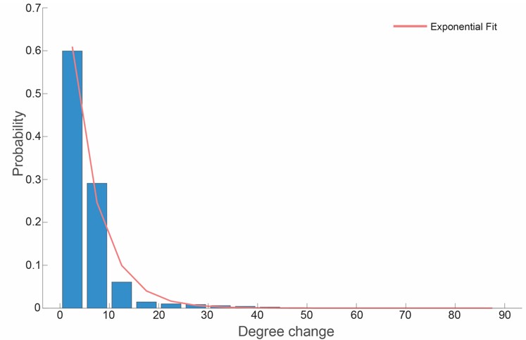
Concretely, the heuristic threshold for SPE-driven remapping (𝜃<sub>𝑟𝑒𝑚𝑎𝑝</sub>) is set to 5 bits, allowing for small miss-convergence during recall in the Amari–Hopfield model. For RPE-facilitated remapping, the threshold is set to 𝜃<sub>𝑁𝐺</sub> = 0.7, making the agent sufficiently sensitive to abrupt environmental changes and enabling it to explore some candidate contexts after RPE-facilitated remapping. This simple thresholding scheme is adequate for our largely deterministic simulation setting, where contextual switches are rare and occur abruptly in an otherwise stable and unambiguous environment.
Importantly, our goal in this work was not to achieve Bayesian optimality. Mice and likely humans in certain settings often deviate from optimal inference. Instead, we focus on the qualitative remapping-related processes that support goal-directed planning following epistemic errors. We have clarified this scope in the revised manuscript.
“In the framework of reinforcement learning, our model can be mapped onto a Bayesian-adaptive model-based architecture in which contextual state serves as the root of Monte Carlo tree search (Guez et al., 2013) in a simple, largely stable environment with noiseless and unambiguous sensory stimuli, and only occasional abrupt changes. In this setup, prediction errors arise from the agent’s lack of experience or due to abrupt environmental changes. … However, these conceptual similarities are qualitative rather than quantitative. The goal of this work is not to achieve Bayesian optimality, but rather to show qualitative remapping-related processes that support goal-directed planning following epistemic errors.”
“Note that we set the remapping threshold 𝜃<sub>𝑟𝑒𝑚𝑎𝑝</sub> = 5 bits to allow for small miss-convergence during recall in the Amari–Hopfield model.”
“Note that we set 𝜃<sub>𝑁𝐺</sub> as 0.7 to make the agents sufficiently sensitive to abrupt environmental changes and enable exploring some candidate contexts after RPE-facilitated remapping.”
(2) Improvement: start describing each task specification in explicit model-based RL terms, then explain how the environmental specification translates into agent operations. Be explicit about what about the process is inferential, in particular, sources of uncertainty.
Thank you for this important suggestion. Following your recommendation, we revised the manuscript to describe each task explicitly in model-based RL terms. For each task, we now identify the relevant sources of uncertainty, which arise either from imperfections in the agent’s internal model of the environment or from occasional abrupt switches in task rules. We also explain how the agent infers the hidden state from experience to construct an appropriate context representation, enabling the model to perform the task successfully.
(3) A lot of seemingly arbitrary model choices need additional computational and biological justification; the description of the process is fundamentally an algorithmic one, which includes a lot of if-then type of operations: the dynamics of different elements of the circuit switch between "initialization to landmark/other", "error detected/not", different forms of plasticity on/off etc and it is not discussed in way how this kind of global coordination of different processes is supposed to be orchestrated biologically; e.g. as far as I understand the sequential structure in H activity is largely hardcoded rather than an emergent property of the learning+neural dynamics.
Thank you for this important suggestion. We have made a concerted effort to clearly describe the biological context and the relevant literature motivating each of our algorithmic assumptions. Notably, as highlighted in Fig. 1F, we emphasize that the sequential structure in H activity emerges as a consequence of the agent’s exploration and learning. We also explain how the two remapping mechanisms concatenate sequence segments to support long-term planning and to predict both stimuli and rewards.
About Fig. 1F
“At the beginning of learning, hippocampal segments are not connected, and H yields only short sequences that generate immediate actions and short-term predictions. As learning continues, the three-factor Hebbian plasticity rule concatenates these segments, thereby creating longer sequences that reflect the task structure (Figure 1F).”
About “initialization to landmark/other,”
“While the history-based initialization was introduced to select contextual state based on the history input from H (episodic), the landmark-based initialization was introduced to terminate the episodes that would otherwise continue indefinitely. Biologically, the landmark-based initialization corresponds to the operation of anchoring a contextual state to salient environmental landmarks - such as an animal’s nest - that serve as clear reference points.”
About “error detected/not,”
“Based on the source of prediction errors, we consider two types of remapping: sensory prediction error (SPE)-driven remapping and reward prediction error (RPE)-facilitated remapping (Figure 1C). SPE-driven remapping is triggered when the mismatch between the predictive inputs from H to X and externally driven sensory inputs exceeds a threshold (see Materials and Methods), causing X to either transition to a different contextual state or form a new one (Figure 1D). RPE-facilitated remapping is more likely to be triggered when the agents execute an action plan following a hippocampal sequence marked by a no-good indicator. The no-good indicator indicates that the action plan, i.e. the hippocampal sequence, has recently been associated with negative reward prediction errors, possibly due to environmental changes (see Materials and Methods). It then facilitates the exploration of alternative hippocampal sequences (Figure 1E). ”
About “different forms of plasticity on/off”
“We used different learning rules for the intra-hippocampal synaptic weights depending on withinepisodic and between-episodic segments.”
“Within-episodic connections, i.e., state-coding to transition-coding synapses, are constantly updated in a reward-independent manner … This modeling is inspired by behavioral time scale plasticity in the hippocampus (Bittner et al., 2017), in which synaptic potentiation occurs for events that are close in time regardless of reward, and such plasticity is believed to support the formation of place cells, etc..”
“Between-episodic connections, i.e., transition-coding to state-coding synapses, are constantly updated in a reward-dependent manner … This is supported by the finding that dopaminergic neuromodulation gates LTP, enabling preferential consolidation of reward-associated experiences (Lisman and Grace, 2005; Takeuchi et al., 2016).”
(4) Improvement: Justify individual design choices by biology whenever possible; in the absence of such justification, provide at least a computational rationale for each such model choice. Additional justification for the neural substrate of different prediction errors.
Thank you for pointing this out. Following the advice, we have added the computational objectives behind each algorithmic component in addition to the biological motivations described above. In particular, we have completely updated Fig. 1 to help readers better understand the key remapping mechanisms in our algorithm: SPE-driven and RPE-facilitated remapping.
About the Amari-Hopfield model
“We employ the Amari–Hopfield model because it allows multiple contexts to be stably maintained and selected in response to stimuli and can be trained via Hebbian plasticity. We assume that similar computations are carried out in prefrontal and entorhinal cortical circuits in the brain.” “As one possible biological implementation, we consider that Context selection in X as the brainwide evoked potential during which bottom-up information may be integrated with top-down signals to select the current context (Mohanty et al., 2025). In this case, it takes several hundred milliseconds for the contextual states in X to settle (Massimini et al., 2005).”
About the default matrix
“This contextual state is set as a default context, ensuring that the X module assigns a unique contextual state to each environmental state. Biologically, one possible interpretation is that this default context corresponds to modality-specific innate representations in prefrontal regions (Manita et al., 2015).”
About state-coding neurons and transition-coding neurons
“The state-coding neurons receive input from X and represent the current contextual state, while the transition-coding neurons send output to X and predict the next contextual state after an action ... One possible biological grounding for this functional separation is that entorhinal cortex provide contextual inputs to CA3, and CA3 and CA1 generates predictions of next state through its recurrent architecture (Chen et al., 2024).”
About the no-good indicator
“No-good indicator is introduced to transiently suppress previously established sequences that have not been recently rewarded, without devaluing them. This no-good indicator facilitates RPEfacilitated remapping (see RPE-facilitated remapping section) that leads to exploration of different contextual states in X and sequences in H. The no-good indicator is inspired by recent findings in the ventral hippocampus, where dopamine D2-expressing neurons of the ventral subiculum selectively promote exploration under anxiogenic contexts (Godino et al., 2025).”
(5) In particular, the temporal scale at which processes unfold with reference to behavioral time scale actions is fundamentally unclear: what determines the time scale of a sequential element? What stitches them together? What is the temporal relationship between H and X operations? At what time scale do actions happen in terms of those operating scales? How does this align with what is known about hippocampal dynamics during behavior?
(6) Improvement: make the time scales of different aspects of the process explicit in the text, potentially with additional graphic support.
Thank you for the questions and suggestions. In this work, we model the agent’s behavior in an abstract grid-world environment with discrete time steps, as is common in classical RL. At each time step, the agent observes a sensory stimulus, makes a plan, and executes an action based on it. The action induces a state transition in the environment. Accordingly, the model includes a single fundamental timescale: the environmental (behavioral) time step.
The modeled brain dynamics in both X and H are similarly locked to this environmental clock. As clarified in Fig. 1F, each sequence segment corresponds to one behavioral time step. These segments are then chunked based on reward events, enabling longer-horizon planning and prediction.
The agent’s cognitive operations at each behavioral time step are summarized in Fig. S1. Briefly, the agent infers the contextual state X from the current stimulus and its stimulus history, generates a sequential action plan H with predictions using chunked sequence segments, and then follows the plan when it is sufficiently promising. In addition, when sensory or reward prediction errors occur, the agent reorganizes the synaptic-weight parameters of the context selector and sequence composer. Once the agent becomes familiar with the environment, H typically generates an extended action sequence along with predictions of future stimuli and the resulting reward. The agent then executes this sequential plan, bypassing step-by-step context estimation by X, until a prediction error triggers remapping.
The revised manuscript includes the following additions.
“For simplicity, the environment is defined in discrete time, and agents move through environmental states characterized by distinct external stimuli. The model operation relies on the environmental (behavioral) time step. At each time step, the agents perform contextual state estimation by Context selector and activate a corresponding hippocampal neuron. Then, this hippocampal neuron initiates sequential activity based on hippocampal synaptic connectivity. Each hippocampal sequence represents a planned course of action and is used to predict a series of external stimuli. … The hippocampal sequence from which actions are generated is updated upon a reward. After the action execution, the agents repeat the process by selecting the current contextual state. As the agents become familiar with the environment, hippocampal sequences that enable future predictions to become longer, and contextual state estimation by Context selector becomes less frequent. The algorithmic flow chart of our model is described in Figure S1.”
(7) As far as I understand it, the existence of splitter cells is directly inherited from the task specification, and to some extent the same can be said about the lap cells; please explain what can be understood from the model simulations that goes beyond what was put into the inputs/reward function for each experiment. Emphasize numerical results that are counterintuitive or where additional predictions about the dynamics come directly from simulating the model but would have been less obvious beforehand.
The existence of splitter cells in our model is not inherited from the task specification. Instead, it emerges directly from the hippocampal module retaining sensory history (namely, whether the agent approached from the left or right arm), independent of reward structure or other task details. When sensory history is removed from the sequence composer (and, consequently, from the context selector), splitter-cell representations disappear.
To develop lap-cell representations, immediate sensory history alone is not sufficient. The sequence composer must chunk episodic segments based on rewards to support sufficiently long action plans (i.e., history dependence) that span the multiple laps required by the task. The planning horizon - the length of action sequences - typically increases as animals learn a task. This progressive development of hippocampal sequences and their dependence on reward yields experimentally testable predictions. Notably, as we clarified in Fig. S2, the required sensory history length must also be learned adaptively: if it is too short, the agent cannot solve the task, whereas if it is too long, learning becomes unnecessarily slow.
In the revised manuscript, we explicitly described the emergent process of splitter cells and lap cells as follows.
About splitter cells
“A second contextual state at S2, X2β, was generated through SPE-driven remapping at the second visit of S2 (second trial) due to history mismatch… In our model, the transition-coding neurons exhibit right/left turn-specific firing at S2 after learning is complete (Figure 2E, I), replicating the emergence of splitter cells.”
About lap cells
“the task environment changes again and the agents are rewarded for two laps, …. Either the shortest transition, ..., or the one-lap transition, …, is no longer rewarded, which triggers another RPE-facilitated remapping and exploration. During exploration, a history mismatch occurs …, and the contextual states for the second lap … are generated. Finally, the rewarded transition of contextual states and corresponding sequence… is reinforced (Figure 3B).”
“This task can also be solved by simply preparing temporal contexts with three steps of sensory history (n=3), which is the minimal number to solve this task. (see Materials and Methods for Model-free learning). However, it takes much longer to find the correct transition for solving the 1-lap task than our model because it involves an excessive number of states (Figure S2).”
“As the agents become familiar with the environment, hippocampal sequences that enable future predictions to become longer, and contextual state estimation by Context selector becomes less frequent.”
(8) The partitioning of H subpopulation into current input vs predictive subpopulations seems to fundamentally deviate from known CA1 properties like theta phase processing, where the same neurons encode information about recent past, present, and future at different moments in time within a theta cycle. The existence of such populations (especially since they come with distinct plasticity mechanisms and projection patterns) seems like a strong avenue for validating the model experimentally.
(9) Improvement: biologically justify the two subpopulations, discuss neural signatures of this distinction that could be used to identify such neurons in experiments
We thank the reviewer for bridging our model with biological circuits.
First, we would like to clarify that we do not claim that our H module corresponds to CA1 specifically.
Rather, we assume that within the broader hippocampal loop (EC–DG–CA3–CA1–EC), subpopulations emerge that preferentially encode the current contextual states and the transitions to the next contextual states. This assumption reflects our hypothesis that the hippocampus implements a mechanism for predicting the next context given the current one. Importantly, this functional separation does not contradict known theta-phase coding in which the same neurons can represent past, present, and future information at different phases of the theta cycle.
As a possible biological grounding, we particularly emphasize the CA3–CA1 projection. Recent studies have shown that CA1 representations exhibit a temporal delay relative to CA3 activity (Chen et al., 2024), suggesting a circuit-level mechanism by which predictions of upcoming contextual states may be computed based on the current context. In this framework, state-coding and transition-coding functions could be assigned to CA3 and CA1, or dynamically expressed through their interactions. Based on our model, we make testable experimental predictions. Specifically, we predict that neural representations in CA3 and CA1 should precede contextual switching in tasks such as alternation or multiple-lap tasks, and that perturbing CA3–CA1 computations would impair task performance.
Please note, however, that our model does not characterize the sequence composer’s activity at such fine-grained neuronal timescales. Instead, we model the computation it performs in abstract time steps corresponding to the grid states (e.g., while the animal is at a corner of the maze).
We have added these points to the Discussion to clarify the biological interpretation and to suggest potential experimental validations of the proposed subpopulation distinction as follows.
“Our model posits that the Sequence composer corresponds to computations within the hippocampus. As a biologically plausible projection, we consider the CA3–CA1 circuit, where contextual inputs from regions such as the PFC and EC provide the current contextual state to CA3, enabling the recurrent CA3–CA1 architecture to generate predictions of the next contextual state. Consistent with this idea, the temporal lag in CA3→CA1 transmission suggests a functional gradient in which CA3 represents present-oriented information while CA1 carries more futureoriented predictions (Chen et al., 2024), and neurons in both CA3 and CA1 exhibit action-driven remapping and encode action-planning signals (Green et al., 2022). Our framework, therefore, predicts that changes in CA3→CA1 population activity precede behavioral switching in contextdependent alternation in Figure 2 or multi-lap tasks in Figure 3, and perturbation of this input will degrade the behavioral performance.”
“While we used an abstract, grid-like state space with discrete time, an important direction for future work is to model its activity at finer-grained neural timescales, such as theta cycles (Foster and Wilson, 2007; Wikenheiser and Redish, 2015).”
(10) The flexibility of the new solution in terms of learning contexts with variable temporal horizons seems an important feature of the model, but one poorly demonstrated in the existing numerical experiments. Could more concrete model predictions be generated by designing an experiment targeted specifically for such scenarios?
Thank you for raising this point.
As we showed in Figure S2, in environments with variable temporal horizons, our model performs better than model-free learning (Q-learning) that incorporates temporal context.
To further demonstrate this point, we added a new task in Figures 3G and H, in which the 1-lap task and the 2+ lap task are alternated. Our model exhibits rapid switching between these tasks, regardless of differences in sequence length or temporal horizon. We added the following text.
“To demonstrate the advantage of our model in a rapidly switching task that requires different history lengths, we show that an agent trained on both the 1-lap and 2-lap tasks can flexibly alternate between them in a reward-dependent manner (Figure 3G), selectively engaging hippocampal sequences of different lengths according to the current task context (Figure 3H). Together, these results illustrate how hippocampal lap-like representations emerge through learning and enable flexible context switching across tasks with distinct temporal demands.”
In such a scenario, a subjective representation of laps in the hippocampus is the key to solving the task. As we responded to points (8) and (9), neural representations, especially in CA1, are expected to bifurcate between the 1-lap and 2-lap conditions, and this bifurcation would precede and critically govern the animal’s behavior.
(11) I found figures confusing/uninformative, specifically in making it explicit what is external task structure and what is the agent's internal representation of it; as a result it is not clear what of the results is trivially inherited from the task specification and what is an emergent property of the model; e.g. Figure 2A described external transition specification according to world model but it is unclear to me if Figure 2B shows the ideal agent state representation across context or a graphical summary of what the agent actually learned from the sensory experience described in A; from the text. Figure 2F is supposed to describe a property of the emergent representation, but what is shown is another cartoon... etc.
We appreciate the reviewer’s insightful comments regarding the clarity of our figures.
To clarify the neural representation of the agent and how it links to the action, we have revised Figure 2 and the descriptions in the main text.
First, Figure 2A schematically depicts the external stimulus as being determined solely by the task. In this task, animals must keep track of the immediately preceding state (S1 or S3) to correctly choose between S4 and S5 upon reaching S2. Without such a memory of prior states, an agent would have no basis for distinguishing which action is appropriate, and therefore cannot selectively move to S4 and S5. Therefore, any reinforcement learning model that does not incorporate at least a onestep state history cannot solve the task.
To solve the task, S2 must be represented as two distinct contextual states depending on the previous state. Figure 2B therefore illustrates an example of internal representation that separates S2 into X2α and X2β: transitions from S1 to S2 are internally represented as X1 → X2α, whereas transitions from S3 to S2 are represented as X3 → X2β. Although the sensory inputs provided to the model correspond only to the task-defined states in Figure 2A, the combination of the sensory input with contextual states in Context selector successfully achieves this contextual representation of X2α and X2β (see Figure 2C, D). Also, the hippocampal neurons in Sequence composer indicate the next contextual states given the current contextual states, i.e., X2α→X4 and X2β→X5 (see Figure 2E). Thus, combining Context selector and Sequence composer successfully achieves the task requirement indicated in Figure 2B.
Regarding the reviewer’s concern that Figure 2F (now Figure 2I) appeared to be another cartoon, we have revised the panel to clearly display our result. These results demonstrate that some hippocampal neurons in our model encode the transition from X2α→X4 and X2β→X5. The updated figure clarifies that our hippocampal neurons functionally work similarly to the splitter cells in Wood et al., 2000.
(12) Improvement: use visuals and captions. Make it clear what is a cartoon, what is a model specification, and what is an actual result. Replace/complement algorithmic cartoons in Figure 1 with a description of the actual result.
Thank you for raising this point.
As we explained in the previous point (11), we added Figure 2D and Figure 2E for displaying the actual neural activity, and the corresponding annotations in the manuscript, e.g, X2α. Also, we revised the cartoons of our model description in Figure 1 to better describe our model structure.
(13) Map between model and experimental results is poorly justified: in particular the nature of sensory inputs is not clearly specified, and how the experimental manipulations (e.g. MEC input disruption) map into model manipulations is not intuitive and no justification is provided for the choices beyond that the model ends up matching the experiment by some metric. Also, not clear why a tradeoff of neural resources as implemented in the model makes sense for the clinical case and how this hypothesis deviates from alternative Bayesian accounts invoking imperfections in inference (e.g. relative strength of priors vs likelihood as reported by e.g. P.Series's group, or issues with hierarchical inference more generally along R.Jardri's work).
Thank you for raising this important point. We have revised the manuscript to clarify the mapping between model components, sensory inputs, and the experimental manipulations, and to further justify the clinical interpretation.
About sensory inputs
First, each environmental state in our model is represented as a binary (0/1) pattern. We have added Figure 2D to explicitly illustrate these sensory stimuli and how they are provided to the context-selection module.
About mapping between model components and brain circuits
Functionally, we speculate that Context selector (X) corresponds to computations carried out in the prefrontal cortex (PFC) and entorhinal cortex (EC), and Sequence composer (H) corresponds to the hippocampus. Inputs from the PFC are thought to reach the hippocampus via the EC. Therefore, suppression of MEC→hippocampus inputs in Sun et al. (2020) naturally maps onto blocking a subset of the inputs from X to H in our model.
We clarified this correspondence in the revised manuscript and now explicitly justify why this manipulation matches the biological experiment.
Relation to Bayesian theories
We agree that Bayesian accounts have provided influential explanations of psychiatric symptoms by invoking imperfections in inference, such as imbalances between priors and likelihoods (e.g., work by P. Series and colleagues) or disruptions in hierarchical inference (e.g., work by Jardri and others). Our model complements these frameworks by explicitly incorporating sequential structure and context remapping. Rather than treating priors as static or fixed-weight quantities, our model allows contextual representations to be dynamically reorganized based on prediction errors over time. In the SZ-like condition, we assume that an excessively expanded context domain increases the influence of internally generated contextual predictions, causing them to override sensory inputs and resulting in maladaptive behavior with hallucination-like percepts. Importantly, this effect reflects not only stronger priors but also excessive generation and competition of contextual states, leading to unstable and non-reproducible remapping. In contrast, in the ASD-like condition, sensory-weighted context representations limit the ability to flexibly incorporate newly introduced contexts, causing the model to perseverate on an initially learned context and thereby reproduce inflexible behavior. We added a schematic illustration in Figure 5B and expanded the Discussion to clarify this point.
“When the stimulus domain is relatively underrepresented, the reconstruction of contextual state in the Amari-Hopfield network tends to infer contextual states based on the context domain rather than the stimulus domain. Consequently, it converges to an incorrect attractor that is not assigned to the current environmental state, thereby increasing perceptual error for external stimuli (hallucination-like effects). Moreover, SPE-driven remapping and the corresponding synaptic plasticity occur more frequently. In contrast, when the stimulus domain is overrepresented, the Amari-Hopfield network rarely assigns multiple contextual states to a given environmental state, leading to an overuse of default contextual states (see Figure 5B and Materials and Methods). ”
“Our model also provides an algorithmic-level account of psychiatric symptoms by changing the relative weighting of sensory-encoding versus context-coding neurons. This implementation is analogous to Bayesian theories linking priors to psychiatric symptoms. In SZ, hallucinations and delusions have been modeled as arising from overly strong top-down priors (Powers et al., 2016) or circular inference, which leads to erroneous belief formation (Jardri et al., 2017; Jardri and Denève, 2013). In our model, we used an underrepresented stimulus domain to increase the relative influence of internally generated context representation in context selection. Crucially, this implementation does not simply strengthen priors but induces excessive generation and competition of contextual states, leading to frequent yet non-reproducible remapping of hippocampal contextual activity and a failure of learning to converge despite repeated experience. In ASD, it has been argued that abnormally high sensory precision reduces the updating of expectations (Karvelis et al., 2018) or leads to sensory-dominant perception, which has been interpreted as weak priors (Angeletos, Chrysaitis, and Seriès, 2023; Lawson et al., 2014; Pellicano and Burr, 2012). In our framework, we used an overrepresented stimulus domain to increase the relative influence of external stimulus representations in context selection. Importantly, our model captures not only sensory-dominant processing emphasized in previous studies, but also a distinctive impairment in flexibly utilizing newly introduced contexts, reflecting a failure of context reconstruction and resulting in persistent inflexible behavior. Thus, our conjunctive modeling of sensory and context processing complements Bayesian accounts of psychiatric symptoms and provides a mechanistic explanation for the role of sensory processing in maladaptive, inflexible behavior. ”
(14) Improvement: justify choices, explain in more detail relationships with computational psychiatry literature.
Thank you for pointing it out. As we explained in the previous point (13), we justified our model choice in the revised version.
Minor comments:
(1) Typos: "algorism" (pg2), duplicate Sun reference.
Thank you for finding the typo and the missing reference. We revised accordingly.
(2) Unclear statements from Methods:
-
"preparing temporal context with three histories" not sure what is meant by this.
-
"... state estimation by the context-selection module becomes less frequent." (Methods/Overview): what is the mechanism?
-
"default pattern" and failure to converge: What is the biological basis for them?
-
Why is the converter function used on some occasions but not others?
-
"new contextual state is prepared": What does that mean?
We thank the reviewer for pointing out several unclear statements in the Methods section.
- “preparing temporal context with three histories”
We now explicitly state the formal description of three histories in the Methods as follows.
“the state is defined by the recent n-step transition history of task state (i.e. 𝑠<sub>𝑘</sub><sup>(𝑛)</sup> =(𝑆<sub>𝑘</sub>,𝑆<sub>𝑘−1</sub>, ⋯,𝑆<sub>𝑘−𝑛</sub>)<sup>𝑇</sup> , where 𝑠<sub>𝑘</sub><sup>(𝑛)</sup> is the temporal context state, and 𝑆<sub>𝑘</sub> is the environmental state at time 𝑘). We changed n from 0 to 3.”
- “state estimation by the context-selection module becomes less frequent”
In our model, context selection is performed every time the agents execute an action sequence generated by Sequence composer. As learning progresses, the Sequence composer comes to predict distant future states and executes coherent action sequences based on these predictions. When no unexpected errors are encountered during execution, context estimation is suppressed, resulting in less frequent context selection. We modified the manuscript as follows.
“After the action execution, the agents repeat the process by selecting the current contextual state. As the agents become familiar with the environment, hippocampal sequences that enable future predictions to become longer, and contextual state estimation by Context selector becomes less frequent. The algorithmic flow chart of our model is described in Figure S1.”
In biological systems, it is reported that the frontal cortex shows sensory modality-specific representation without prior learning (Manita et al., 2015). We refer to these innate modalityspecific sensory representations as the default pattern. In the early stages of learning, we assume that no stable contextual representations have yet been formed in the brain, and therefore, a default pattern uniquely driven by external stimuli is used as the context representation. Even during intermediate stages of learning, the context selector may fail to converge to a specific state. In such context-uncertain environments, it has been reported that agents often rely on previously learned or habitual action choices (psychological inertia), which is evident in ASD patients.
“This contextual state is set as a default context, ensuring that the X module assigns a unique contextual state to each environmental state. Biologically, one possible interpretation is that this default context corresponds to modality-specific innate representations in prefrontal regions (Manita et al., 2015).”
“This default implementation is analogous to psychological inertia, particularly under uncertainty (Ip and Nei, 2025; Sautua, 2017), which has been reported to be more pronounced in ASD patients (Joyce et al., 2017).”
- Why is the converter function used only in some cases?
The converter function A(stim → context) was introduced to compose the default pattern (one-toone mappings between stimuli and contexts) as we described above. In other cases, the Hopfield dynamics were used to select contextual states; therefore, we did not use the converter function.
- “new contextual state is prepared”
Thank you for pointing this out.
The term “prepared” was inaccurate. We revised it to “generated”.
In the case of remapping, we assumed that X generates a new random neural activity pattern in its contextual domain and stores it as a new contextual state. We described this process as “a new contextual state is generated”.
(3) Please explain the mapping between hippocampal sequences to actions in more detail for each task.
We appreciate the reviewer’s request for clarification. Below, we provide additional explanations point by point.
Mapping between hippocampal sequences and actions
In this research, we defined action as the transition from one environmental state to another environmental state. The hippocampal sequences predict the transition of environmental states; therefore, they correspond to a set of action plans from the current environmental state. In the revised manuscript, we added the formal definition of environmental states and actions in each task.
- Why 9 attempts before rejection?
These repetitions ensure adequate exploration of the contextual states in X and the episodic sequence in H before committing to an action. Increasing the number of attempts excessively causes the reward value function  to be dominated by a single highest-scoring sequence, thereby causing excessive exploitation and narrowing behavioral variability. While the exact number 9 is not critical—the qualitative results are robust to moderate changes—we selected this value because it provides a good balance between exploration and exploitation and produces the clearest visualizations in our figures. We have clarified this in Method below.
“We set the number of attempts before rejection to nine, providing a balance between exploration and exploitation and serving as a good compromise for visualization.”
- Why all the variations on Hebbian learning?
We consider three loci of plasticity in our model: the X module, the H module, and their reciprocal connections. Within the H module, synaptic connections that link episodic segments—specifically from transition-coding neurons to state-coding neurons—are assumed to follow a reward prediction error–dependent, supervised form of Hebbian learning. This choice reflects the need to selectively reinforce transitions that lead to successful outcomes. In contrast, all other synaptic updates in the model are assumed to follow reward-independent, activity-based Hebbian learning. These learning rules support the unsupervised formation and stabilization of contextual representations and action execution.
In addition to the basic Hebbian rule, we introduced biologically motivated constraints, such as upper and lower bounds on synaptic weights and heterosynaptic depression, which weakens nonpotentiated synapses. Importantly, these mechanisms do not alter the fundamental nature of Hebbian learning but increase the stability of our model.
(4) For Q learning: please clarify "the state is defined by the recent transition history of task state.
As you suggested, we clarified the statement by adding the following sentences in Method. “To highlight the advantage of our model, we compared it to the Q-learning with temporal contexts, namely, the state is defined by the recent n-step transition history of task states (i.e. 𝑠<sub>𝑘</sub><sup>(𝑛)</sup> =(𝑆<sub>𝑘</sub>,𝑆<sub>𝑘−1</sub>, ⋯,𝑆<sub>𝑘−𝑛</sub>)<sup>𝑇</sup> , where 𝑠<sub>𝑘</sub><sup>(𝑛)</sup> is the temporal context state, and 𝑆<sub>𝑘</sub> is the environmental state at time 𝑘.”
(5) What is the purpose and biological justification for the NG addition to RW?
Thank you for raising this point. The prediction-error–based update of each sequence’s value function 𝑅 alone cannot distinguish between two fundamentally different cases:
(a) the value of a sequence has genuinely decreased, or
(b) the sequence remains useful, but it is just not appropriate in the current context. This distinction is essential for modeling context-dependent switching of behavioral strategies. To address this, we introduced the No-good (NG) indicator. NG allows the agent to temporarily mark certain sequences as unsuitable without altering their long-term value, thereby facilitating short-term exploration of alternative sequences. In other words, NG provides a mechanism for transiently suppressing a previously valid sequence in case of contextual changes, while preserving the underlying value learned in past experiences.
This mechanism is consistent with several lines of biological evidence. First, extinction learning after fear conditioning does not erase the original fear memory but instead forms a new memory trace, known to be stored in the medial PFC (Milad & Quirk, 2002). This suggests that animals may switch to a different contextual representation rather than simply downgrading the value of the conditioned stimulus, supporting the idea of temporarily suppressing a sequence without modifying its intrinsic value.
Second, recent studies in the ventral hippocampus show that dopamine D2–expressing neurons in the ventral subiculum promote exploration specifically under anxiogenic contexts (Godino et al., 2025). This finding is consistent with the short-term exploratory behavior enabled by our NG mechanism. Thus, we added the following statement to the manuscript:
“No-good indicator is introduced to transiently suppress previously established sequences that have not been recently rewarded, without devaluing them. This no-good indicator facilitates RPEfacilitated remapping … that leads to exploration of different contextual states in X and sequences in H. The no-good indicator is inspired by recent findings in the ventral hippocampus, where dopamine D2-expressing neurons of the ventral subiculum selectively promote exploration under anxiogenic contexts (Godino et al., 2025).”
Together, these biological findings provide a conceptual basis for modeling NG as a contextsensitive, transient modulation that encourages exploration without overwriting previously learned sequence values.
(6) Missing details about H network size
Thank you for pointing it out.
We used 300 neurons for H. We indicated it as below.
“We model the hippocampus with an N = 300 binary recurrent neural network.”
(7) S1 figure: learning is slower even in the early, easy phases of learning when the temporal dependence should not matter; how are learning rates calibrated across models?
Thank you for raising this point. In our model, the learning rate was fixed at 0.15, whereas the control model (now shown in Figure S2) uses a higher learning rate of 0.4, independent of temporal context.
Regarding why learning appears slower even in the early, easy phases, when the number of temporal contexts increases, the size of the state space expands. This broadening of the state space makes it more time-consuming to identify and reinforce the appropriate state transitions. This is especially evident in easy phases because the temporal context prepared in the model is excessive to the number of temporal contexts that the task requires.
Importantly, unlike the control model, which postulated a fixed number of temporal contexts, our model gradually increases the number of temporal contexts depending on prediction error. This adaptive mechanism allows the model to achieve fast learning during early, easy phases while still enabling more complex learning in later phases.
Reviewer #2 (Recommendations for the authors):
(1) "Hippocampal neurons show sequential activity...." The authors should include more classical references for hippocampal sequential activity at this point, too.
Thank you for your suggestion. We added the citations below
Skaggs and McNaughton, 1996; Wilson and McNaughton, 1993
(2) "...called remapping" also here, please reference classic work (Bostock, Muller, ...)
As suggested, we added the citations below
Bostock et al., 1991; Muller and Kubie, 1987
(3) "Several theoretical models..." What I miss here are models that explain remapping by inputs from the grid cell population, and/or the LEC (see Latuske 2017 for review), still widely considered the standard mechanism. Also, the models by Stachenfeld et al. 2017, Mattar and Daw 2019, and Leibold 2020 specifically address context dependence. Accordingly, "A comprehensive model that can explain the formation of context-dependent hippocampal sequences of various lengths through remapping, while relying on a biologically plausible learning process,..." somewhat overstates the novelty of the current paper.
Thank you for pointing this out and for suggesting relevant citations. We agree with the reviewer that inputs from MEC and LEC to the hippocampus constitute a fundamental mechanism underlying remapping. However, in our view, a key open question in the remapping field is how MEC and LEC estimate the current context and convey this information to the hippocampus in a manner that supports goal-directed behavior. While previous studies have addressed remapping at the representational level and the hippocampal sequence at planning, the overall relationship between remapping, reinforcement learning, and planning has not yet been explained within a single unified model. In this work, we propose a simple and biologically plausible model that integrates an Amari–Hopfield network for context selection with hippocampal sequences, providing an account of coordination under goal-directed behavior. To more accurately position the novelty of our contribution, we have revised the manuscript as follows.
“While previous works have explored hippocampal sequential activity for planning (Jensen et al., 2024; Mattar and Daw, 2018; Pettersen et al., 2024; Stachenfeld et al., 2017) and hippocampal remapping for contextual inference (Low et al., 2023) separately, they have yet to elucidate how these two aspects jointly enable flexible behavior. A simple biologically plausible model-based reinforcement learning model that uses the Amari-Hopfield model for context selection and hippocampal sequences of various lengths as a state-transition model for long-horizon planning, relying on remapping driven by prediction errors to form state representation, would thus provide valuable insights into the neural mechanisms underpinning context-dependent flexible behavior.”
(4) Please properly introduce nomenclature "C2α, C2β, S2,...." S is sometimes used for stimulus, sometimes for location (state?), or even action?
Thank you for pointing it out. We acknowledge that the annotation of Cn (e.g., C1, C2…) was not straightforward. Therefore, we changed the annotation to Xn (e.g., X1, X2, …) in order to indicate the contextual state of X.
We define Sn (e.g., S1, S2…) as the external input given by the environment and represented in stim. domain of X, while Xn (e.g., X1, X2…) is the subjective contextual state generated by the agent and represented in the context domain of X. As a reference, we added the neural representation of X in Figure 2D and added the following text below.
“The neural activity of X at each contextual state is shown in Figure 2D, where the environmental states (e.g., S1, S2…) are represented in the stimulus domain, and the contextual states (e.g., X1, X2α…) are represented in the context domain.”
(5) "Our model replicates this result by blocking the synaptic transmission from most of the neurons in the context domain of X to H (Figure 3F).". Does this mean the X module is hypothesized to be in the EC?
Thank you for the thoughtful question. In our model, the X module is intended as a functional abstraction that combines the roles of several brain regions known to contribute to contextual representation, including the prefrontal cortex (PFC) and the entorhinal cortex (EC). Although X is not necessarily meant to correspond to a single anatomical region, we consider it likely that the contextual information represented in X would reach the hippocampus (H) (CA3 and CA1) primarily through the EC. Thus, the experimental manipulation shown in Figure 3F—suppression of medial EC axon at the hippocampus—is interpreted in our framework as weakening the input from X to H.
We added the following texts in the Discussion section.
“We speculate that Context selector is implemented across multiple brain regions with varying degrees of resolution, including a part of the entorhinal cortex and prefrontal cortex.”
“Our model posits that the Sequence Composer corresponds to computations within the hippocampus. As a biologically plausible projection, we consider the CA3–CA1 circuit, where contextual inputs from regions such as the PFC and EC provide the current contextual state to CA3, enabling the recurrent CA3–CA1 architecture to generate predictions of the next contextual state.”
(6) Discussion "model-based reinforcement learning": Please detail where the model is here. In my understanding, the naive agent does not have a model (this would be model-free then?).
Thank you for asking.
Unlike model-free reinforcement learning, where each action is evaluated step by step, we use hippocampal sequences for multiple-step prediction and action planning. This is the “model” in our research. As you mentioned, initially, animals do not have a “model”, but Sequence composer gradually chunks the episodic segments to compose a longer sequence.
(7) "...can change the attractor dynamics in the hippocampus (34)": What is (34)? I also would doubt that one can make such absolute statements about the human hippocampus.
Thank you for pointing out the missing citation. We corrected it accordingly.
Rolls E. 2021. Attractor cortical neurodynamics, schizophrenia, and depression. Transl Psychiatry 11. doi:10.1038/s41398-021-01333-7
(8) "To the best of our knowledge, this is the first model that describes the formation of contextdependent hippocampal activity through remapping and its contribution to flexible behavior." See "Several theoretical models...".
Thank you for pointing this out. We admit that it was an overstatement. We corrected it accordingly.
“To the best of our knowledge, this is the first model that uses associative memory for describing the formation and switching of context-dependent hippocampal activity through remapping and its contribution to flexible behavior.”
(9) "We speculate that the context-selection module is implemented across multiple brain regions..." How would an attractor network be implemented over "multiple brain regions"?
We thank the reviewer for raising this important conceptual question. Context information in realistic environments is likely to have a hierarchical structure. We therefore speculate that multiple brain regions may jointly support context selection by maintaining different levels or components of this hierarchy. In particular, the prefrontal cortex (PFC), medial entorhinal cortex (MEC), and lateral entorhinal cortex (LEC) have all been implicated in representing contextual or task-state information at different levels of abstraction. These regions are known to exhibit attractor-like dynamics and to provide inputs to the hippocampus. Thus, an attractor network spanning multiple regions could arise, with different areas stabilizing distinct components of the contextual representation, depending on the timescale of memory, task demands, or sensory features.
We used the Amari–Hopfield network as a functional abstraction to explain such multi-regional interactions underlying context representation, rather than to provide a one-to-one mapping onto a specific brain region. How region-specific attractor dynamics jointly contribute to maintaining global contextual information and enabling context switches in response to prediction errors remains an important direction for future research.
Methods:
(10) "... agents move through discrete environmental states characterized by distinct external stimuli.": How is this exactly implemented? What is the neural representation of these states, xi? What is the difference to a "landmark"?
We appreciate the reviewer’s thoughtful question regarding the implementation and neural representation of environmental states. In our model, each environmental state is represented as a binary stimulus pattern provided to the stimulus-domain neurons in Context Selector. Specifically, for each state, we constructed a pattern in which half of the neurons are set to 1 and the other half to 0. We chose this design because, in the Amari–Hopfield model, memory performance is maximized when stored patterns contain approximately equal proportions of 0 and 1. For clarity, we have added an illustration of these stimulus patterns in the revised Figure 2D.
Regarding the reviewer’s question about landmarks: in our framework, a landmark denotes an environmental state for which the contextual state is uniquely determined, regardless of the preceding transition history. For simplicity in this study, we designated the initial environmental state in each task (S0 or S1) as the landmark. Importantly, in our implementation, landmarks do not differ from other states in terms of their stimulus pattern; their special role arises solely from the task structure, not from additional sensory properties.
In real environments, what constitutes a landmark likely varies depending on stimulus saliency and the agent’s prior experience. Determining how landmarks should be optimally defined or learned is an interesting direction for future work.
(11) How are different contexts represented for the same stimulus xi^stim?
We added an example of neural activity in X in Figure 2D, illustrating the distinction between the stimulus domain and the context domain. While the activity in the stimulus domain depends on the external stimulus, the contextual domain consists of uncorrelated random neural states. We exploit a key property of the Amari–Hopfield network to associate each contextual state with a given external stimulus.
(12) "...and its stimulus domain ??stim becomes identical to ??xistim ." Does that mean every stimulus is an attractor in the context net? How can that work with only 1200 neurons? Is that realistic for real-life environments? Neuron numbers would need to increase dramatically.
As you mentioned, we assigned each stimulus to a corresponding attractor in the Context selector (X). An Amari–Hopfield network with 1,200 neurons can store approximately 10–20 attractors, which is sufficient to solve the tasks considered in this study. We adopted the Amari–Hopfield network for its simplicity and conceptual clarity; however, in biological neural systems, it is not necessary to construct such rigid attractors for every stimulus. For example, modality-specific neural projections exist in the brain and are sometimes sufficient to form loose attractor states across different stimuli. In addition, the prefrontal cortex is known to support working memory, which may also serve as a form of contextual representation incorporating recent history. Thus, we propose that multiple brain regions cooperate to implement the Context selector.
(13) How are WHX and WHH initialized?
Thank you for pointing this out.
We set the initial condition of all W to 0. We added the following text in the Method section.
“Note that the initial synaptic weights of 𝑊<sup>𝐻𝑋</sup> and 𝑊<sup>𝑋𝐻</sup> are all 0.”
(14) It is unclear why the hippocampus separates into state and transition neurons. Why cannot one pattern serve both purposes?
Thank you for asking about this important point.
The reason why we prepare two kinds of hippocampal neurons is that state-coding neurons represent the current contextual state, and transition-coding neurons predict the following contextual state under the current contextual state. These two separations enable it to predict multiple scenarios under the current contextual state and to choose a sequence most suitable in the environment.
We rewrote the following sentences in the manuscript.
In result section,
“In Sequence composer, there exist two types of neurons: state-coding neurons, which represent each contextual state, and transition-coding neurons, which encode transitions to successive contextual states given the contextual state indicated by the state-coding neurons”
In Method section,
“The state-coding neurons receive input from 𝑋 and represent the current contextual state, while the transition-coding neurons send output to 𝑋 and predict the next contextual state after an action i.e., T(𝑋<sub>𝑘+1</sub>|𝑋<sub>𝑘</sub>,𝑎<sub>𝑘,𝑘+1</sub>).”
(15) "the agents execute actions according to this sequence." How are the actions defined? Are they part of the state?
We thank the reviewer for raising this important point. In our model, an action is defined as the transition from a given environmental state to the next environmental state. To avoid ambiguity, we have added a formal mathematical definition of actions for each task in the revised manuscript. In our framework, the transition-coding neurons in Sequence Composer (H) predict the upcoming environmental state, and thus the hippocampal sequence intrinsically contains the representation of an action. Consequently, the sequence generated before actions functions as the agent’s internal action planning process.
(16) "Because the input source for the state-coding neuron and the transition coding neuron differ (the former is selected from ??, while the latter is selected from ??), the same hippocampal neuron could occasionally be used for both state-coding and transition-coding across different contextual states. This is evident when an excessive number of contextual states are prepared, especially in the SZ condition. This phenomenon degrades state estimation at X (eq.3)." I have no idea what you want to convey here, .... and how is state estimation related to Equation 3?
We appreciate the reviewer’s feedback and agree that our original explanation was unclear. Our intention was to clarify why context estimation deteriorates specifically in the SZ condition.
In our model, state-coding neurons in the hippocampus represent the current contextual state, and transition-coding neurons predict the next contextual state given the current contextual state. Under normal conditions, these two sets of neurons remain sufficiently distinct, allowing accurate prediction of the upcoming contextual state, which is conveyed to X. However, when an excessively large number of contextual states are stored in the SZ condition, representations in the hippocampus begin to overlap. As a result, some hippocampal neurons are inadvertently recruited for both state-coding and transition-coding across different contextual states. This overlap disrupts the H’s ability to accurately predict the next contextual state.
This degraded prediction directly affects the state-estimation process in X (Eq.3), because Eq.3 relies on receiving an accurate predicted next state from H. When this signal becomes ambiguous, X may converge to an incorrect contextual state, potentially mimicking hallucination-like inference errors.
We have rewritten the relevant passage in the manuscript to clarify this mechanism as follows.
“When the number of contextual states increases - particularly in the SZ condition - representational overlap arises between hippocampal state-coding and transition-coding neurons.
This overlap makes the prediction of the next contextual state by the transition-coding neurons unreliable. The degraded prediction from H, in turn, corrupts the initial condition for context selection in X (Eq. 3), leading to hallucination-like behavior.”
(17) The figures hardly show simulated activity. Consider displaying more neuronal simulations to help the reader grasp the workings of the model.
Thank you for your suggestion. We indicated the neural activity of X and H in Figures 2D and 2E, respectively, to show the overview of our model.
(18) Figure 5: What is the "Hopfield count"?
Thank you for pointing this out. The definition of the Hopfield count was ambiguous. We added an explicit explanation of “context selection” and its possible outcomes (correct association, hallucination-like, and default contexts) in Fig. S1. To clarify our claim, we replaced the countbased measure with the probability of selecting hallucination-like and default contexts during context selection. Accordingly, we removed the term “Hopfield count” and revised the caption of Figure 5 as follows.
“The result of context selection (see Figure S1). The probability of wrong stimulus reconstruction (hallucination-like effects) is plotted in red, and the probability of default context usage due to failures in context reconstruction (see Materials and Methods) is plotted in blue.”
(19) Figure 6: Consider moving this upfront.
Thank you for the suggestion. We moved Fig.6 to Fig.S1 and introduced it earlier in the manuscript.
Reviewer #3 (Recommendations for the authors):
I was a bit confused about the implementation, which may not be autonomous, meaning there are numerous stages that require intervention from outside the X-H network (see Figure 6). It seems that the X network might wait to converge before providing input to H, rather than having the entire network evolve in parallel. There are also aspects to the implementation that seem rather ad hocsuch as the "no-good indicator".
Thank you for the thoughtful comments. We would like to clarify several points regarding the implementation and its biological motivation.
First, regarding the concern that the X–H interaction may not be fully autonomous:
In our framework, the convergence time of the X module under external sensory input is assumed to be on the order of several hundred milliseconds, consistent with the timescale of stimulus-evoked cortical population dynamics observed in biological systems. Especially when hippocampal input is present, X does not need to explore the full attractor landscape. Instead, it quickly settles into an attractor located near the hippocampal cue, which substantially shortens the convergence time.
Second, although our current implementation proceeds in an algorithmically sequential manner for clarity, we do not intend to imply that the brain performs these steps sequentially. Biologically, the states of X and H are expected to co-evolve and mutually constrain each other through recurrent interactions. The sequential algorithm in the model is therefore a practical choice for implementation, not a theoretical claim about strict temporal ordering in the neural system.
Finally, the “no-good indicator” is introduced to suppress hippocampal sequences transiently and thereby accelerate switching behavior. Our no-good indicator is most consistent with the biological findings on D2-expressing neurons in the hippocampus. We added the following text below.
About the no-good indicator
“The no-good indicator is inspired by recent findings in the ventral hippocampus, where dopamine D2-expressing neurons of the ventral subiculum selectively promote exploration under anxiogenic contexts (Godino et al., 2025)”
Besides the hippocampus, similar mechanisms—temporary suppression of recently visited or lowvalue attractor states—have been proposed in biological decision-making and working-memory literature, providing conceptual support for the no-good indicator in our model.
After exposure to a new context, a new memory/context is stored in the X network. As the storage of a new memory requires synaptic plasticity, this step would presumably take a significant amount of time in an animal.
Thank you for raising this important point. We agree that the formation of a new memory or context requires synaptic changes, and it is well established that processes such as tagging during wakefulness and consolidation during sleep take considerable time. However, once a context has been learned, switching between contexts can be achieved just by moving between attractors in the X network. This mechanism allows for rapid, context-dependent behavior without requiring new synaptic modifications each time. Our study focuses on this aspect of fast context-dependent switching rather than the initial memory formation.
My understanding is that the Amari-Hopfield network should be evolving in continuous time and not be binary. But there were no time constants mentioned, and the equations were not provided, and it seems that the elements of X were binary units, rather than analog. This should be clarified.
Thank you for the comment.
Although there are models with continuous firing rates and continuous time (Ramsauer et al., 2021), the original Amari-Hopfield model uses binary neurons operating in discrete time steps. As we answered the comments (5) and (6) from Reviewer 1, we considered only a discretely timestepped environment for which the timescale is arbitrary. At each environmental state where the current contextual state is selected, it typically takes about ten iterations for the conversion of the Amari-Hopfield network.
In the text, we added the following text.
“For simplicity, the environment is defined in discrete time, and agents move through environmental states characterized by distinct external stimuli.”
Figure 3 is aimed at replicating the lap cell finding of Sun et al, 2020. In panel E, a comparison is made between the data and the model. Are the cells in the model the entire population of H neurons (state and transition), or just a subset? Does the absence of the "ghosts" (the weaker off diagonal responses seen in the experimental data) imply that the network is not encoding that it is in the same location, but a different lap? Why is there not any true sequentiality (i.e., why do all H units go on at once)?
Thank you for your insightful comments. Throughout this study, we used 300 neurons for the Sequence composer (H); however, for simplicity, we constrained the model such that only a single H neuron was active at each time point. As a result, most other neurons remained silent. Accordingly, in Fig. 3E, we display only neurons with firing activity, and silent neurons are not shown.
As you correctly inferred, hippocampal neurons in our model encode lap identity rather than the same physical location across laps. This design choice reflects our focus on hippocampal neurons representing contextual states, rather than place-coding neurons, as only the former contributes directly to contextual behavior in our framework. As shown in Fig. 3E, hippocampal neurons exhibit clear sequential activity with “episode-like” representations corresponding to individual laps. Nevertheless, we believe that incorporating a mixture of context-coding neurons and place-coding neurons is an important direction for future work, as illustrated in Fig. S3.
We revised the caption of Fig. 3E as follows.
“E, The comparison of (Left) lap cells in the hippocampus in the 4-lap task (Sun et al., 2020) and (Right) our results of active neurons in the H module.”
Typo "but also makeS predictions".
Thank you for pointing this out. We revised it correctly.