Baldwin et al. described the relationship between the stratosphere and the troposphere. Changes to stratospheric circulation can, in turn, affect tropospheric weather patterns. This study notes that the North Atlantic Oscillation (NAO) was the pattern most strongly related to wintertime changes in stratospheric temperatures and circulation.

Shindell et al. described the importance of modeling stratospheric atmosphere dynamics to improve predictions of global climate conditions. They also determined that it was possible to program climate models to simulate climate patterns like the Arctic Oscillation when including greenhouse gas concentrations. This suggested that greenhouse gases can influence regional climates.

This was a pivotal paper in helping to develop a method of correcting satellite temperature data. By using satellite measurements over the early 1990s during the time of the Mount Pinatubo eruption, Reynolds and Smith were able to factor out the volcanic aerosols for a more accurate measurement of global temperatures.

This paper reviews the recent history of North Atlantic changes in convection and deep water formation. Waters are mixed downwards in the Greenland and Labrador Seas, but this study found that these locations are currently at opposite convective extremes.

The authors proposed that atmospheric forcings (such as the North Atlantic Oscillation) are influencing the location and quantity of water sinking into the deep ocean.

"Approaches to studying the ocean's role in climate can be divided into two types: understanding and modeling the ocean as part of the fully coupled climate system, and observing, quantifying, and modeling the dynamics of the ocean itself."

This comes from Lazier's chapter "The Oceans" in the book Natural Climate Variability on Decade-to-Century Time Scales, available online: https://www.nap.edu/read/5142/chapter/5#234

One of the elements of a global climate model is a simulation of CO₂ circulation.  However, models that begin in pre-industrial times include so much data that computers take a long time to complete the simulation. To decrease processing time, scientists sometimes set the start date of the simulation later, but this introduces error into the model. The authors of this paper found a way to account for this error (called the "cold-start" error) and discussed the implications for the climate models used by the IPCC. 

Levitus had previously performed a very similar study that focused on the temperature and salinity of the North Atlantic. More measurements have been collected since this study in 1989, making it possible to examine more of the world's oceans and to update the scientific understanding of what was going on in the North Atlantic.

Nitta and Yamada used global ocean temperature data to discover that, since the late 1970s, surface temperatures were rising in the tropics, particularly in the eastern Pacific and the Indian Ocean. Their research suggests the changes in ocean temperature may have contributed to a change in climate patterns, affecting the Pacific-North American in particular.

For example, if a temperature profile was taken on Feb. 19th, for each depth in that profile the authors subtracted out the average value for all Februaries over the last 50 years for each depth point. This removes the seasonal temperature changes from the data-set, allowing the authors to focus on the long term variability instead.

Antonov investigated temperature changes in the North Atlantic and North Pacific oceans within the depth range of 300 to 3000 meters over the years 1957–1981.

He found that, while the North Pacific did not change temperature in deeper areas, it cooled between 300 and 500m. On the other hand, over the same period, North Atlantic ocean temperatures increased in the 800 to 2500 meter layer.

The Intergovernmental Panel on Climate Change (IPCC) is the leading international body for the assessment of climate change. The IPCC reviews and assesses the most recent scientific, technical, and socioeconomic information relevant to the understanding of climate change.

This study utilized the 1995 IPCC report. Updated versions come out every few years, with the 5th and most recent IPCC report published in 2014.

For more information about the IPCC, visit:

https://www.ipcc.ch/index.htm

The Intergovernmental Panel on Climate Change (IPCC) noted in 1995 that humans are influencing the climate. Since the publication of this study in 2000, we have learned even more about the extent to which humans have contributed to climate change. 

In the latest report from 2013, the IPCC was “95 percent certain that humans are the main cause of current global warming.”

In 2018, oil companies like Chevron began admitting in court that human activities are changing the climate.

Read more in Vox: https://www.vox.com/energy-and-environment/2018/3/28/17152804/climate-change-federal-court-chevron

Climate scientists have been working on ways to visualize changing global temperatures. One way is to present a spiraling graphic of monthly temperature data going back to the year 1850, where a series of concentric circles represents incremental increases in global temperature.

When viewed alongside carbon dioxide concentrations emitted by fossil fuels, there is a clear correlation between temperature and carbon dioxide.

Since 2010 when this paper was published, enough evidence has accumulated that 95% of climate scientists agree that climate change is being driven primarily by human activities.

View the animation and read more in the Washington Post: https://www.washingtonpost.com/news/energy-environment/wp/2016/07/28/these-climate-spirals-perfectly-illustrate-the-human-hand-in-global-climate-change/?utm_term=.34a3c771b2e3

Has this hypothesis been proven true since this paper was published in 2000?

Use the National Oceanic and Atmospheric Administration's (NOAA) website to investigate changes in ocean temperatures since this study was published: https://www.nodc.noaa.gov/OC5/3M_HEAT_CONTENT/

The Earth is an interconnected system where conditions in the atmosphere also affect what happens in the oceans. While the authors cannot say for sure that specific climate oscillations are driving the changes in ocean heat content, it is possible to say that changing climates are likely impacting ocean heat content.

Polarity means to have two opposite or contradictory tendencies or aspects. In this case, the North Atlantic Oscillation (NAO) has both a warm phase and a cool phase, and convection (ocean mixing) differs between these conditions.

This 500-mb height (mb stands for millibar, which is a unit for measuring air pressure) is the typical height presented in weather maps. Since most weather occurs roughly around this height in the atmosphere, looking at 500-mb maps of the sky makes it possible to more accurately predict weather events.

Thompson and Wallace did not directly state that the North Atlantic Oscillation (NAO) may be part of the Arctic Oscillation (AO), but they did mention that these oscillations share many similar characteristics.

Thompson and Wallace found that changes in wintertime sea level pressures above the high northern latitudes of Europe and Asia was part of an AO, distinct from the NAO. The AO "resembles the NAO in many respects; but its primary center of action covers more of the Arctic." This means that there are aspects of the climate features which can distinguish between these two climate phenomenon.

Want to see how the 1997 event was different from the El Niño event in 2015-2016?

Check out this Washington Post article: https://www.washingtonpost.com/news/capital-weather-gang/wp/2015/08/13/el-nino-then-and-now-a-side-by-side-comparison-of-1997-and-2015/?utm_term=.48a1ef8932e3

Or read more in the Los Angeles Times: http://www.latimes.com/local/california/la-me-0822-el-nino-1997-20150822-story.html

La Niña is the counterpart to El Niño and involves cooler than average waters across the equatorial Pacific Ocean.

"Both El Niño and La Niña can alter wind and water currents across the globe, causing extreme weather that can kill thousands of people and result in billions of dollars in damage."

The 1998-1999 La Niña event was particularly extreme, causing droughts in the southwest US and thousands of deaths in regions across the globe, including China, Venezuela, Bangladesh, Honduras, and Nicaragua.

Read more in the article by LiveScience: https://www.livescience.com/49572-la-nina-events-increase-climate-change.html

What causes El Niño, how can it affect you, and why is it so hard to predict? Find out in this video from National Geographic:

https://www.youtube.com/watch?v=d6s0T0m3F8s

Reynolds helped develop a method for converting satellite data into accurate temperature measurements. One of the problems with satellite data is that it has to be corrected for anomalies such as dust and aerosols, which can make satellite measurements slightly different from reality. It is possible to get usable temperature data from satellites by accounting for this and correcting the data.

Altimetry is a technique for measuring the height of the surface below the altimeter. Satellites do this by sending a radar pulse to the surface of Earth. The time it takes for the pulse to bounce off the surface and return to the satellite is used to measure height, or altitude. Combined with precise satellite location data, such satellite measurements yield sea-surface heights.

Launched in 1992 as a joint mission of the U.S. and French space agencies, TOPEX/Poseidon was the first major oceanographic research satellite in space. It's goal was to map the topography of the ocean surface.

The sea-level pressure is the atmospheric pressure at a given location in the ocean. Because pressure and temperature are correlated, changes in temperature that result from climate change can, in turn, change sea-level pressure. 

Dickenson et al. analyzed North Atlantic water temperatures and proposed a theory that the variability in deep ocean mixing is related to the regional climate pattern (the North Atlantic Oscillation).

The restart of deep water mixing in the Labrador Sea just southwest of Greenland coincides with a change in phase of the North Atlantic Oscillation. This study notes that climate has a strong impact on the extent of deep water formation (convection) in the North Atlantic Ocean.

Convection is the movement of a fluid due to changes in density, where more dense waters sink and less dense waters rise. Subduction is the term for the downwards movement of a substance, in this case when one water mass moves below another.

The heat content of the atmosphere contributes to the warming of the ocean, so it would seem logical for the surface ocean to warm more quickly than the deep ocean (because the deep ocean is farther from the atmosphere).

However, data suggests that the heat content of the deep ocean is increasing more quickly than the surface ocean. This further suggests that deep ocean circulation is transporting warmth from the surface to greater depths.

There are also time series records of land temperatures. For the last 100 years, many countries have recorded increasing temperatures.

To learn more, check out this Carbon Brief video created by Antti Lipponen: https://www.youtube.com/watch?v=-yIHxOui9nQ

"A global climate model typically contains enough computer code to fill 18,000 pages of printed text; it will have taken hundreds of scientists many years to build and improve; and it can require a supercomputer the size of a tennis court to run."

Running a global climate model can take a long time, even with a super computer (days to weeks). Finding ways to run models more efficiently saves both time and money.

Read more in the Carbon Brief: https://www.carbonbrief.org/qa-how-do-climate-models-work

There are many assumptions that go into creating global climate models. This is because these models must simulate complex interactions between the atmosphere, oceans, land surface, ice, and the sun.

However, as information from real-world sources such as satellites and other measurements accumulates, climate models are constantly refined to increase their power, usefulness, and accuracy. Improved climate models that have been released since this paper was published have made the concern about a sudden increase in atmospheric carbon dioxide less of an issue.

For more about climate models visit Skeptical Science: https://www.skepticalscience.com/climate-models-basic.htm

To accurately predict conditions on Earth, models of ocean currents and circulation are connected, or coupled, with models of atmospheric, ocean, and sea ice dynamics.

Hansen et al. discovered that, between 1979 and 1996,Earth received somewhere between 0.5 to 0.7W/m² of extra energy. As energy can not be created nor destroyed, this extra incoming energy remains in the Earth system and contributes to climate change. 

Levitus et al. found a ∼2 × 10²³ joules warming between the mid-1950s and mid-1990s, which corresponds to a warming rate of 0.3 watts per meter squared.

Thus, the ocean appears to be absorbing nearly half of the total heat that results from the warming of the Earth.

Caused or influenced by human activities.

Warm, salty seawater from the mid-latitudes is transported northward by the Gulf Stream. Once it reaches the higher latitudes near the Labrador Sea, cold air temperatures chill the seawater. This salty, cold seawater is denser than warmer waters, so it sinks and becomes the formation zone for North Atlantic deep water.  

This density-driven process of deep ocean circulation is sometimes referred to as Thermohaline Circulation. "Thermo" refers to temperature and "haline" refers to how much salt the water contains. Both temperature and salinity are key components in determining density.

The North Atlantic is one of the few regions in the world where deep water formation occurs.

The mechanisms causing ocean temperatures to increase are likely the same for every ocean.

Examples include the radiative forcings from volcanic aerosols, stratospheric ozone depletion, greenhouse gases, and solar variability.

The western midlatitudes in this case represent the area between 30° - 45°N and 80° - 40°W. In this area the surface 300 m of the ocean has warmed by 1-2°C from the 1970s to the 1990s (Fig. 3A). This increase is even more extreme in the deeper ocean which has warmed by as much as 8°C (Fig. 3B).

After examining the data in 500 m increments, Levitus and coauthors determined that most of this warming is occurring in the top 1000 m.

In each ocean basin, there have been periods when the heat content has increased and periods when the heat has decreased. However, the overall trend shown by the data is that every ocean basin on the planet has been warming over the last 50 years.

Most of that warming has occurred after the 1950s and 1960s.

It is only in the North Atlantic that the ocean is being warmed at deeper depths. In the Pacific and Indian oceans, warming appears to only occur in the surface 1000m. 

The Labrador Sea is the region between Greenland and Canada around 60°N, 50°W that shows some of the most extreme cooling throughout the water column (Fig. 3B).

Levitus et al. found that the cooling of the Labrador Sea has consistently declined by 1W/m² for every 500m in depth, extending all the way down to 2500 m.

By examining the ocean in distinct depth increments of 500m each, the authors aimed to determine where most of the cooling and heating of the North Atlantic is occurring.

The North Atlantic ocean absorbs a lot of heat, but where is that heat being stored?

The heat that the ocean absorbs does not remain in the surface ocean, but is instead carried to deeper depths by deep ocean convection currents. From the 1970s to the 1990s, the deep water of the North Atlantic has gained more heat than the surface ocean has over the same period.

The authors calculated how much heat is being stored in the deep sea by looking at the cumulative temperature change from 1955-59 to 1970-74, as well as from 1970-74 to 1988-92.

By integrating, or combining, the temperature data for all depths between 0 and 300m and between 0 and 3000 m, the authors aimed to examine where the heat is going - into the surface ocean or the deep ocean.

The likelihood that a relationship between two or more variables is caused by something other than random chance. The data suggest there is a real difference in the temperature values between 1955-59 and 1970-74, as well as between 1970-74 and 1988-92.

A statistical test to compare the means of two groups.

For more information visit: http://www.biostathandbook.com/twosamplettest.html

The waters of the Mediterranean are extremely warm and have high levels of evaporation, causing the sea to be very salty. While Mediterranean waters are typically warmer than in the Atlantic Ocean, the high salinity causes Mediterranean waters to be slightly more dense than surface waters of the Atlantic. Because of this, water that exits the Mediterranean into the Atlantic sinks and flows out into the Atlantic at roughly 1000 m depths.

For more information about the Mediterranean Outflow and to see real Argo float depth profiles visit: http://www.euroargo-edu.org/floatdata.php?float=6901631

Ocean regions between latitudes 50°N and 70°N are subarctic.

In subarctic oceans, there is a large range of temperature variation through the year, with cold winters and moderately warm summers. These latitudes also experience deep ocean mixing due to strong winter storms.

The deep ocean of the North Atlantic cooled between the period 1970-1974 and the period 1988-1992, two decades later. While higher latitudes show this cooling most strongly, the decline in deep water temperatures appears to have occurred through much of the North Atlantic.

A series of 5 years. The later two pentads refers to the periods 1988-1992 and 1970-1974.

The North Atlantic has different water masses with distinctive temperature, salinity, and densities.

The Mediterranean Outflowoccurs at the region where the Mediterranean Sea meets the Atlantic, and has a different enough density to be distinct as it's own water mass.

This figure shows some of the water masses in the Atlantic Ocean from Antarctica (60°S) to the Northern Arctic Ocean (70°N). Image Source: http://www.atmosedu.com/Geol390/Life/OceanCirculation.html

Overall, the deep water of the North Atlantic had higher temperatures during the period 1970-1974 than during a period two decades earlier, from 1955-1959.

The change in heat content from one decade to the next is similar in scale to the shift in heat content that happens over the course of a year due to the change in seasons.

That is, the range of temperature from the highs of summer to lows in winter is similar to the extent of change from one decade to the next.

The deep ocean below 300m is disconnected from the atmosphere and appears to have little influence on climate.

The Pacific Decadal Oscillation (PDO) is typically thought of as a long-lived El Niño-like pattern of Pacific climate variability. Areas of the Pacific Ocean go through alternating patterns of warming and cooling every 10 to 30 years. 

For more information and to see a time series of PDO variability, visit: https://www.ncdc.noaa.gov/teleconnections/pdo/

The repetitive variation of a measurement over time, such as how temperature varies around a central value over time. 

While there are periods of increasing and decreasing heat content in the oceans, with swings happening roughly every two decades, the Pacific Ocean has seen an overall increase in temperature over time.

Occurring roughly every two decades.

In 1998, the North Atlantic ocean was 0.37°C (0.37°F) warmer than the 50-year average.

Has this trend continued since Levitus et al. published this study in 2000?

You can find the answer by examining ocean temperature data available from NASA: https://climate.nasa.gov/vital-signs/global-temperature/

Levitus et al. found that, as time progresses, ocean temperatures increase. Thus, time and ocean temperature are positively correlated.

Much of this ocean warming has occurred since the mid-1970s.

A relationship between two variables such that their values increase or decrease together. As time increases, the heat content of these basins also increases, suggesting these variables are positively correlated.

The measure of the statistical accuracy of an estimate. One of the most common measures is standard deviation, which can be presented as error bars (showing a margin of error) on a graph.

Because the Earth is a spinning sphere, certain wind and ocean currents have formed that make it useful to think of the Equator as a boundary between North and South Pacific waters.

To learn more about how ocean currents are driven by wind, water density differences, and tides, watch this video from the National Oceanographic and Atmospheric Administration (NOAA): https://oceanservice.noaa.gov/facts/current.html

The costs of going to sea add up: the captain, crew, and scientists must have food and income, and the ship must have power. Deploying sensors to great depths in the ocean typically requires that a ship remain stationed in place, taking up time that could be spent heading to port.

Because of the difficulty of reaching it, the deep ocean is still mostly unexplored and is considered by some to be Earth's "final frontier." In addition to studying the unique organisms that thrive deep in the ocean, scientists are also focused on examining how changes in deep sea temperatures affect global climate.

Read more in LiveScience: https://www.livescience.com/30890-ocean-deep-mysteries-exploration.html

Oceanographers typically measure distinct depth levels in the ocean, with more measurements taken in the surface ocean than in the deep ocean.

For the upper 100m, measurements are taken every 5m in depth (i.e., 0m, 5m, 10m, 15m, 20m, etc.). Between 100m and 500m, measurements are taken every 25m (100m, 125m, 150m, 175m, etc.). From 500m to 2000m those measurements are every 50m (500m, 550m, 600m, 650m, etc.). For depths greater than 2000m, then data is collected in increments of 100m (2000m, 2100m, 2200m, 2300m, etc.).

The authors combine 5 years of data into one value, typically by averaging all values. A running composite (sometimes known as a moving or running average) is calculated by creating a series of averages of different subsets of the full data set in order to compare to the original data set.

Calculating a running composite is a common technique used with time series data in order to smooth out short-term fluctuations and highlight longer-term trends or cycles.

For more information on how to calculate a moving average: http://www.statisticshowto.com/moving-average/

The authors calculated temperature anomalies by subtracting the seasonal temperature cycle from monthly data values.

Every now and then a shipboard temperature measurement can malfunction or be used incorrectly, recording temperatures far higher or far lower than what is realistic. These values need to be excluded to accurately study the oceans. To make sure these errors do not affect the study, the authors considered a particular range of data points with cutoffs at the higher and lower end of the range.

Unlike their previous work, the authors used a less strict cutoff for when data values were considered good enough to use in their analysis. This is because they found that some large-scale temperature features were mistakenly being flagged as "bad" data under the stricter cutoff, despite those features being real and measurable events in the ocean.

An anomaly is something that deviates from what is standard, normal, or expected. Here, the authors examine how temperature varies from expected values.

Using data available in the World Ocean Database, Levitus et al. looked at both annual temperature data and average season temperatures within each year (for winter, spring, summer, fall).

However, because temperature changes over the course of a year due to the changing of the seasons (summers are warm, winters are cold), this seasonality must be taken into account when studying the overall change in ocean temperatures. To "objectively analyze" the data, the natural seasonal temperature cycle was subtracted from each data point in order to focus on the trends over time.

For each monthly temperature data point, the average temperature for that month the sample was measured was subtracted. The difference between the data point and the monthly average is called an anomaly.

The authors averaged monthly oceanographic data acquired by ship-of-opportunity and research vessels into annual temperature measurements for every year from 1960 to 1990.

Scientists measure locations on Earth using longitude (180° E ↔ 180° W) and latitude (90° N ↔ 90° S).  Lines of longitude and latitude cross to create a grid across the planet.

For this study, Levitus et al. combined temperature data for every 1° longitude by 1° latitude area of the ocean. Where multiple ships frequented the same location, those multiple data points were averaged into one value for each matching depth.

The ocean is a major carrier of heat. As warm surface currents move towards the poles, they slowly release heat. Once cold and dense enough in the high latitudes, this water sinks and the deep ocean currents carry cold waters to lower latitudes.

Figure from Thompson and Seiber (2011, IJBC).

Due to Earth's tilt, the tropics receive more incoming solar radiation than the poles do, so there is excess warming in the lower latitudes. Wind and ocean currents carry this heat towards the higher latitudes.

This figure shows the balance between average net incoming solar radiation (shortwave) and the heat emitted by earth (longwave radiation) from 90° North to 90° South.

Read more about earth's energy balance here: http://www.physicalgeography.net/fundamentals/7j.html

Radiative balance is when solar energy coming to the Earth is balanced by an equal flow of heat from the Earth into space. If the Earth is in radiative balance, then global temperatures will remain relatively stable.

The study of the atmosphere and weather patterns. Meteorological data is often used to predict the weather.

Because chartered research vessels are expensive and time-consuming to organize, ship-of-opportunity programs use a combination of volunteer commercial and research vessels to collect oceanographic measurements. For example, a shipping vessel can be equipped with sampling instruments that will acquire data while it moves along a normal shipping route.  

The surface ocean is generally thought of as the top 1,000 meters (3,300 feet) of the ocean, which includes the region of rapidly changing temperatures called the 'thermocline'.

As you can see in this NOAA figure, everything below the thermocline is the deep ocean.

It is possible to think of "global warming" as "ocean warming" because so much heat from the atmosphere makes its way into the world ocean.

It is difficult to measure the temperature of the oceans because of how large and deep they are. It is also challenging to track this data over time and examine long-term trends. 

Read more in The Guardian: https://www.theguardian.com/environment/climate-consensus-97-per-cent/2017/jun/26/new-study-confirms-the-oceans-are-warming-rapidly

This figure shows how ocean temperatures have changed in each ocean basin from 0 to 3000m in depth. Due to gaps in temperature data (especially in the 1950s), Levitus et al. used 5-year averages (composites) instead of looking at annual data (as in Figure 1).

The authors found that there is an overall increase in temperatures within each ocean basin. This warming is not consistent, but instead has periods of lower temperatures and periods of higher temperatures.

How does this figure differ from Figure 1 that only looks at 0 to 300m depths?

Specific heat is the amount of heat per unit mass required to raise the temperature by one degree Celsius.

Thus, specific heat is a thermodynamic property of seawater expressing how heat content changes with temperature. A substance's specific heat also depends on temperature, pressure, and salinity.

CLIVAR stands for "Climate and Ocean: Variability, Predictability and Change." The goal of CLIVAR is to further our understanding of the oceans and climate.

For more information visit: http://www.clivar.org/about

Monotonic means to neither increase nor decrease.

As the warming is not monotonic, this means there are periods where temperature has increased and other periods where temperatures have decreased.

All of the world's oceans have been warming since at least the 1970's according to measurements by ships and research vessels.

From the data available, it appears the Atlantic and Pacific started warming before the Indian Ocean, but this result could be due to the fewer number of data points collected in the Indian Ocean.

While the whole ocean warmed 0.06 C between the 1950s and 1990s, Levitus et al. found that the surface ocean (the top 300 meters or 984 feet) warmed by 0.31 C.

All of the world's oceans combined - the Atlantic, the Pacific, the Indian - have warmed by 0.06°C overall between 1948 and 1998.

But have the oceans all warmed equally, or have some basins or depths warmed more than others?

Scientists use the "~" symbol to mean "approximately." This means the world ocean's heat content increased by approximately 2x10²³ joules.

2x10²³ joules is the same as 200,000,000,000,000,000,000,000 joules, or a 2 with 23 zeros following it.

The average.

Using satellite pictures and infrared satellite imagery, it is possible to assign hurricanes into different categories depending on characteristic patterns.

As a tropical cyclone develops, there tends to be certain characteristics depending on the intensity of the storm. Those visual characteristics in the swirls of clouds and moisture change in a predictable fashion as a storm system strengthens.

This technique has been compared to aircraft measurements in order to test its accuracy and has some of the highest accuracy in gauging hurricanes in the North Atlantic and North Pacific Oceans.

Check out NOAA's website for more information: http://www.aoml.noaa.gov/hrd/tcfaq/H1.html

The Dvorak scheme is a method of determining storm intensity based off satellite images and certain characteristics. Tropical cyclone patterns used to estimate intensity come from 1) the “shear” pattern, which examines how tilted a hurricane may be from the upper to lower atmosphere, 2) the “curved band” pattern of how the clouds swirl around a cyclone, 3) the “central dense overcast” pattern as in how thick the cloud cover appears, and 4) the “eye” pattern that examines the shape of the storm's center.

Here is an image presents some of the common patterns seen during tropical cyclone formation along with their Dvorak-assigned intensities:

A Dvorak T-Number of 1.0-2.0 is considered a tropical depression, 2.5-3.5 is a tropical storm, 4.0-4.5 represents a category 1 hurricane, 4.5-5.0 is a category 2, 5.5 is considered a category 3, with 6.0-6.5 representing category 4, and T numbers of 7.0-8.5 correspond to category 5 hurricanes.

In this study, William Gray discusses the seasonal variability in Atlantic hurricane frequency.

He found that during years with strong El Nino conditions in the Pacific, there were fewer hurricanes, hurricane days and tropical storms in the Atlantic. He also discovered that when stratospheric winds (at 30 mb in the atmosphere) were from an easterly direction, there tended to be fewer storms.

In contrast, more tropical storms and hurricanes occurred during non-El Nino years as well as when stratospheric winds blew from a westerly direction.

Thus global and regional climate oscillations in addition to upper atmosphere weather dynamics influence hurricane frequency.

Knutson and Tuleya explored how the choice of climate model and convective wind parameters simulating hurricanes can impact the model results. By running experiments examining higher carbon dioxide futures using different climate models and different wind and atmospheric assumptions, the authors looked at whether different models produced the same results.

They found that "nearly all combinations of climate model boundary conditions and hurricane model convection schemes show a CO2-induced increase in both storm intensity and near-storm precipitation rates." They also found a "gradually increasing risk in the occurrence of highly destructive category-5 storms" if global climate continued to warm.

Based on this study, it appears that most climate models tend to produce similar results regardless of differences in certain background parameters and assumptions.

For this study, William Gray examined measurements of upper atmospheric conditions which had only recently become available from over the tropical oceans. Using about a decade's worth of airplane and sensor readings, Gray noticed that cyclone storms develop under certain conditions with regard to temperatures and atmospheric moisture content.

Development of storms appears to be due to the combination of surface winds converging due to frictional forces in addition to conditions inhibiting atmospheric vertical mixing (such as specific wind shear and cloud conditions). Under certain atmospheric conditions, warm oceans and evaporation-condensation reactions of water can concentrate energy into a cyclonic system and cause a hurricane to form.

Using a simple model that takes the thermodynamic attributes of the atmosphere into account, Emanuel determined that if carbon dioxide concentrations doubled there would be a "40–50% increase in the destructive potential of hurricanes".

This is due to the well-studied heat-trapping potential of carbon dioxide which contributes to a warming climate and increasing sea surface temperatures. Warmer waters in turn alter atmospheric pressures and wind speeds. Thus on a theoretical basis using knowledge of atmospheric gases and their relationship to temperature, a warmer world is likely to produce more destructive hurricane events.

Landsea and coauthors compared the record of hurricane activity in the Atlantic with other climate records of sea level pressures, wind, climate oscillations (like the El Niño-Southern Oscillation), African West Sahel rainfall, and Atlantic sea surface temperatures.

They found that variability in the background climate state of the region affects the frequency, intensity and duration of Atlantic hurricanes.

With improved understanding of the large-scale climate conditions of the Atlantic and how regional climate changes over multi-decadal timescales should improve our ability to predict hurricane activity.

Trenberth and coauthors wrote this paper in order to summarize the environmental controls on precipitation events and to point out how climate models were not yet considering all the variables influencing precipitation.

Since "climate change is certainly very likely to locally change the intensity, frequency, duration, and amounts of precipitation" we need to be developing models which can accurately reproduce these types of changes if we want to accurately predict how the water cycle may vary as climate changes.

In this perspective piece "Uncertainty in Hurricanes and Global Warming" Trenberth notes that while the effects of human-driven climate change have already begun altering the environment in hurricane formation regions, it is not yet possible to connect changes in climate to the number of storms forming.

Trenberth suggests that instead of focusing on just the number of storms and the tracks they move along, the bigger scientific question is how hurricane attributes such as intensity and rainfall are changing in today's world.

Goldenberg and coauthors studied "The recent increase in Atlantic hurricane activity: causes and implications."

After examining hurricane data from 1944 to 2000, these authors also found that there has been an increase in cyclone activity and the number of major hurricanes since 1995. They attribute the greater storm activity on increases in North Atlantic sea-surface temperatures and decreases in vertical wind shear.

These changes in storm activity appear to coincide with changes in the climatic state of the Atlantic, specifically in how the Atlantic responds with regard to El Nino and La Nina conditions that vary on the timescales of a few decades. Due to the current climate of the North Atlantic, Goldenberg and coauthors predict "the present high level of hurricane activity is likely to persist for an additional ∼10 to 40 years."

The trends noted here appear to be real and not due to an error in the analysis, instruments, or observations.

Airplane weather measurements have been extensively compared against satellite data, especially for the North Atlantic, and has been shown to well estimate hurricane categories through satellite imagery.

As all the satellite images were analyzed in a similar fashion (the Dvorak scheme of cloud pattern comparison), the trends of increasing category 4 and 5 hurricanes are not caused by some problem with the analysis and thus appear to be driven by an environmental trend.

After examining decades worth of satellite data on storms, it is now more likely a category 4 or 5 hurricane will form than how many used to occur in the 1970's. Thus the number of intense, life-threatening storms appears to have increased over the 35 year record of satellite data analyzed in this article.

The study cited here by Kossin and Velden found that there was a latitudinal bias in the way scientists were utilizing the Dvorak scheme to estimate storm intensity. At different latitudes, atmospheric pressures remain stable at different heights (e.g. air expands in warmer temperatures, near the equator).

There was no bias in estimating atmospheric pressure around the 23°N, but estimates for the latitudes both closer to the equator and farther north to the poles needed to be reconsidered.

They found that the pressure estimates based on satellite images needed correcting, but that estimates of wind speeds was still useful and accurate enough.

Velden and co-authors came up with an algorithm based technique for examining satellite imagery and cataloging storm systems. Their "Objective Dvorak Technique" is a modified version of the original Dvorak scheme which uses patterns in winds and moisture content to rate a storm on its intensity and characteristics.

Instead of humans eye-balling characteristics, now computers do the calculations for us to determine storm behavior.

The authors are referring to the change from visual, human eye-balled categorizations of satellite images to computer-based algorithms.

The transition from humans to computers in cataloging storm system removed some of the personal subjectivity between tropical storm analysts.

Greg Holland studied a subset of global data in order to see how enhanced observational technology has improved the detection of intense tropical storms.

He found that prior to the use of satellite imagery to recognize storms, records tend to underestimate the true number of events. This may be due to the amount of storms which form and remain far offshore which did not make it into historical records. Thus in the 1960's when satellites really started getting widespread usage for tracking weather, scientists "saw" more hurricanes than previously reported.

The article they reference is "On the quality of the Australian tropical cyclone data base" where Greg Holland studied a subset of global data in order to see how enhanced observational technology has improved the detection of intense tropical storms.

He found that prior to the use of satellite imagery to recognize storms, records tend to underestimate the true number of events. This may be due to the amount of storms which form and remain far offshore which did not make it into historical records. Thus in the 1960's when satellites really started getting widespread usage for tracking weather, scientists "saw" more hurricanes than previously reported.

There appear to be more category 4 and 5 hurricanes forming in the 2000's than there were thirty years ago according to analyzed satellite data.

This trend towards an increased frequency of some of the strongest, most intense storms has also been a result of other studies and model simulations.

The authors used satellite imagery and characteristic wind and moisture patterns in order to gauge the intensity of storms and hurricanes.

This method of gauging hurricane intensity has been tested against aircraft sensor measurements and does a solid job of accurately recognizing hurricane characteristics.

As part of weather missions, certain aircraft literally penetrate to a storm's center in order to drop sensors that can transmit information about the storm back to the National Hurricane Center.

This supplies data on environmental conditions of different storms in order to directly compare against satellite images.

For more information, check out the "Hurricane Hunters" tab on NOAA"s website: https://www.noaa.gov/explainers/hurricane-forecasting

The Department of Defense in conjunction with the National Oceanic and Atmospheric Administration (NOAA) have access to a fleet of aircraft to conduct hurricane/tropical cyclone reconnaissance, general surveillance, and research missions.

The aircraft take measurements of geographic position, pressure height and altitude, wind direction and speeds, temperature and dew point temperature among others. These data are collected anywhere from every 30 seconds to every half hour while in flight. Up to five reconnaissance missions may go out in a day.

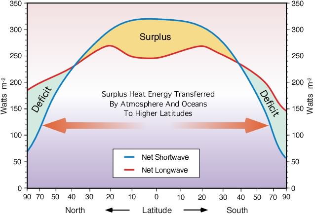
This image shows some of the types of aircraft used by the U.S. to study hurricanes: Image from NOAA's Hurricane Hunters

There has been an increase in the number of storms that reach a category 4 or 5. This increase has occurred in every ocean basin: the Pacific, Atlantic, and Indian Oceans.

There are fewer category 1 hurricanes in the 2000's relative to the other category storms than there were in the 1970's.

A monotonic decrease means that for the whole of the record, there has been a decline in the percentage of category 1 storms. There were few if any periods where percentage values were constant or increasing.

Based on the satellite data from the 1970's to 2004, it is not possible to link warming ocean temperatures with a change in the number of hurricanes per year.

While the North Atlantic may be showing an increase in hurricane days with warming temperatures, the same is not happening in other ocean basins.

The number of hurricanes and storm days in the west Pacific Ocean increased from the mid 1970's to the early 1990's before declining to 2004.

Sea surface temperatures have been increasing in the west Pacific from the 1970's to 2000's. So there is not a clear relationship between storm frequency and sea surface temperatures for this ocean region.

There have been changes to the number of hurricanes and storm days per year that occur on the order of ten years or less in the eastern Pacific Ocean.

Examining Fig. 3, the eastern Pacific (EPAC) has a maximum number of storms occurring around 1984 and again near 1993. Between 1993 and 2004, the number of hurricanes and storm days has been declining.

Check out Fig. 1 again. Temperatures in the eastern Pacific have increased from the 1970's to 1992 before beginning to decline around 1993 to 2001.

A pentad is a 5-year period of time.

"Covariability" is the measure of how much two variables vary together. In this case, the authors are looking at whether ocean temperatures and hurricanes vary together.

A confidence level is the probability that the value of a parameter falls within a specified range of values. In this case, the authors are 99% certain that there is an increasing trend in the number of North Atlantic hurricane and storm days.

Of all the ocean basins examined, only the North Atlantic had a trend of increasing hurricane and storm days from 1970 to 2004.

Between 1990 and 2000, there was a decade-long period of more frequent cyclonic storm days.

Both the number of hurricanes and the number of storms, there was no statistical trends in the data. Thus it is not possible to state that the number of hurricane and storm events has increased over the period 1970 to 2004.

Total hurricane days = number of days where surface wind speeds remained higher than 33 m s–1.

Tropical storm days = number of days where surface wind speeds remained between 18 and 33 m s–1.

The Saffir-Simpson scale utilizes a hurricanes sustained wind speeds in order to try and estimate potential property damage.

Category 3 hurricanes and higher have the potential for significant loss of life and damage.

Check out the definitions for each category at the National Hurricane Center website: https://www.nhc.noaa.gov/aboutsshws.php

The term "hurricane" is given to systems that develop over the Atlantic or the eastern Pacific Oceans. They are called "typhoons" in the western North Pacific and Philippines. Lastly, they are called "cyclones" in the Indian and South Pacific Ocean.

These authors used satellite data from 1970 to 2004 in order to examine cyclones and hurricanes in every tropical ocean basin.

They examined: 1) number of storms and hurricanes 2) number of storm days 3) hurricane intensities

Most of the data examined came in the form of best track data archived in hurricane warning centers.

Using satellite data it is possible to track the development and movement of hurricanes. The tracks that hurricanes progress upon are recorded and stored in online archives typically run by governmental agencies.

For example, the National Hurricane Center compiles past track maps which allow us to look at U.S. landfalling major hurricanes from 2001-2010:

Check out some of the other tracks and data available here: https://www.nhc.noaa.gov/data/?#tracks_all

The U.S. Department of Defense agency responsible for issuing tropical cyclone warnings for the Pacific and Indian Oceans does so through the Joint Typhoon Warning Center, which utilizes satellite data in order to estimate the risk of typhoons and hurricanes of the Pacific and Indian Oceans.

To check out if any storms are currently being watched, visit their website: http://www.metoc.navy.mil/jtwc/jtwc.html

For example from September 19th, 2018:

These authors used a statisical test called the Kendall Test (also known as the Mann Kendall Trend Test or M-K Test) in order to determine if there was a trend through time in the data.

For more information visit: http://www.statisticshowto.com/mann-kendall-trend-test/

From the 1970's to the 2000's, sea surface temperatures have been increasing through time for every ocean basin except the southwest Pacific Ocean. The statistics performed (Kendall Test) suggest this trend is real and significant.

According to a CBS News article from 2017:

Numerous studies have "confirmed the importance of sea surface temperature in controlling hurricane maximum intensity, and suggest an increase of 2-3 percent in hurricane strength per 1 Celsius degree increase in sea surface temperature under favorable conditions."

However directly connecting individual storms to the increasing sea surface temperatures related to climate change is still a difficult proposition. This is because "on top of the day-to-day intensity fluctuations due to local environmental conditions, hurricanes may also possess chaotic behaviors that cause their intensity to highly vary."

Read this article at CBS News: https://www.cbsnews.com/news/does-climate-change-affect-hurricanes/

"Interannual" means occurring between years or from one year to the next.

Thus this is stating that there is variability in hurricanes from one year to the next due to the effects of large scale climate conditions.

One of the reasons for why it is so difficult to predict a change in hurricane frequency is due to intrinsic biases and assumptions built into the climate models being utilized.

While the 2012 Intergovernmental Panel on Climate Change reports that tropical hurricanes are likely to decrease in frequency with increasing temperatures, the storms that do form are likely to see increased winds and rainfall.

This article from Climate Central in 2013 details one study by MIT researcher Kerry Emanuel which found that tropical cyclones are likely to become both stronger and more frequent in the years to come, which is contrary to previous findings.

Read the article here: http://www.climatecentral.org/news/study-projects-more-frequent-and-stronger-hurricanes-worldwide-16204

In order for a hurricane to form, there are multiple environmental conditions that must align. First off, an area of low pressure over the tropical ocean known as a "pre-existing disturbance" must form in an environment favorable for development.

Other conditions include: Ocean temperatures must be above 26°C (80°F), sufficient moisture in the air, enough distance from the equator to establish a cyclonic movement, and atmospheric conditions that support thunderstorm development are necessary for a hurricane to develop.

For more information visit the University of Rhode Island's 'Hurricanes: Science and Society' site: http://www.hurricanescience.org/science/science/hurricanegenesis/

The relationship between a change in temperature and a change in saturation vapor pressure is nonlinear, as in when plotted against each other the results do not form a straight line. This means that an increase in temperature causes an increase in vapor pressure much larger than would be the case in a linear relationship.

Here is an example of how temperature affects vapor pressure: Image from Lyndon State College.

The year 2004 was the "Year of the Four Hurricanes" when Hurricane Charley, Frances, Ivan and Jeanne made landfall in Florida and caused billions of dollars worth of damages.

Since then there have been improvements to electric grids, shelters, forecasting abilities and the ability to communicate which should hopefully save lives in future hurricanes.

The Florida newsgroup Sun Sentinel reviews these 4 hurricanes, what has been improved since, and what still needs fixing. Read their article here: http://interactive.sun-sentinel.com/2004storms/

A causal relationship means that the data suggests that one variable has a direct influence on another.

Climate models are created using complex mathematical representations of the interactions between the atmosphere, oceans, land surface, ice, and the sun. Such models are tested against real world data and once they can realistically reproduce past climate conditions, then they are used to simulate future conditions.

Different models might use different mathematical equations in their calculations, some of which may have large uncertainties involved for certain environmental interactions. As our understanding of the environment improves, the models also improve in their predictive capabilities but because of the complexity of the global Earth environment there is still more to discover about the world around us.

For more about the reliability of climate models, visit Skeptical Science: https://www.skepticalscience.com/climate-models.htm

The atmosphere is not all uniform. There are layers of the atmosphere which differ in gas concentrations, temperatures, and density.

The troposphere is the lowest layer and extends from sea level up to about 6.2 miles (10 km) into the atmosphere. This region is where weather occurs and the layer above is known as the stratosphere.

Image from the University Corporation for Atmospheric Research.

Vertical wind shear is a change in wind speed or direction with change in altitude. So if wind moves rapidly upwards or downwards, it would be a vertical shear.

Strong vertical wind shear tends to inhibit cyclone development, but may also extend the lifetimes of individual thunderstorms.

In order to be called a hurricane (or a typhoon or tropical cyclone) the storm system must reach sustained winds of 74 miles (119 km) per hour or higher.

Meteorologists use the generic term 'tropical cyclone' to describe a rotating, organized system of clouds and thunderstorms that originates over tropical or subtropical waters. These large scale air masses tend to spiral around an atmospheric region of low pressure.

Different places around the world will call these storm systems by different terms: hurricane, typhoon, or tropical cyclone.

For more information visit: https://oceanservice.noaa.gov/facts/cyclone.html

According to the National Oceanic and Atmospheric Administration (NOAA) hurricane "storms are given short, distinctive names to avoid confusion and streamline communications."

The US began using female names for hurricanes in 1953 and started including male names in 1978.

For more information visit NOAA's website: https://oceanservice.noaa.gov/facts/storm-names.html

According to the National Weather Service, the official hurricane season starts on June 1 for the Atlantic and May 15 for the Pacific, both ending on Nov. 30. August through November are peak months with a high storm likelihood.

For information about the 2018 hurricane season, check out this article from LiveScience: https://www.livescience.com/57671-hurricane-season.html

"The Ocean is essential to life on Earth. Most of Earth's water is stored in the ocean. Although 40 percent of Earth's population lives within, or near coastal regions- the ocean impacts people everywhere. Without the ocean, our planet would be uninhabitable."

Check out this NASA's Goddard video about the ocean: https://www.youtube.com/watch?v=6vgvTeuoDWY

By comparing a modeled map using every data point available and comparing that map to one that excludes outliers exceeding 3 standard deviations, the authors realized they were actually excluding some ocean temperature features that occurred. Thus by changing the data cut-off to 6 standard deviations it was possible to more accurately model ocean conditions.

Areas where heat are being stored and the ocean warmed over the two decade period between 1970-74 and 1988-92 are colored in red with positive values. Ocean regions which are releasing heat and thus becoming colder over that period are colored in blue with negative values.

Figure A focuses on the surface 300 m of the North Atlantic and suggest the higher latitudes, roughly 45°N to 70°N, were releasing heat while the regions below 45°N warmed over the two decades.

Figure B looks at where heat is accumulating over the two decades from the surface down to 3000 m. From 1970-74 to 1988-92 the Labrador Sea (southwest of Greenland) and the subarctic region were cooling while the western mid-latitudes (20°N to 45°N) warmed.

Most of the heat storage is occurring at depths below 300 m.

This figure focuses on the annual anomalies in heat content of the surface 300 m of the ocean basins. Every year from 1948 to 1998 is plotted as a bar on these charts of temperature anomalies. Positive values indicate an above-average warm year, while negative values indicate a below-average cool year.

Which ocean basins show a trend from cold, negative values to warm, positive values? Are the trends in one direction consistent over the full 50 year record or only for shorter periods of time?

Levitus and coauthors found:

• The Atlantic and Indian oceans overall show an increasing trend towards warming temperatures with time, a positive correlation.

• Temperatures were cooler before the mid-1970s and warmer after that.

• Of all the ocean basins, the North Atlantic ocean during the year 1998 saw the warmest temperatures of the last 50 years.

By broadening the cutoff criteria the authors of this study were able to distinguish real-life changes in ocean temperatures. Their previous data cutoff of 3 standard deviations (which are a measure of variance around a mean), was too strict and deleting real data points.

Broadening the pool of what was considered "good" or "realistic" data to 6 standard deviations was necessary in order to properly document temperatures that actually occurred in the oceans.

The areal extent of warming is colored in red, while the blue color represent areas that cooled between the time periods. The black contour lines are labeled with the exact extent of temperature change, where the thickest black line represents no change in temperature (0°) over the roughly 20 years between pentads.

Figure A is presenting how temperatures have changed between the late 1950s and early 1970s in the North Atlantic at a depth of 1750 m. Much of the North Atlantic appears to be warming, excluding the Mediterranean Outflow area.

Figure B presents the temperature change between the early 1970s and the 1990s. The Labrador Sea appears to have cooled substantially, with cooling also occurring in most of the rest of the North Atlantic.

Nerem and coauthors found that during the 1997–1998 El Nino event there was a 20 mm rise and subsequent fall of mean sea level was observed. As these changes occurred alongside a rise and fall of global mean sea surface temperature anomalies, their work suggests the observed mean sea level change is mostly caused by thermal expansion.

Thermal expansion means that as water warms it expands to take up more space, which causes sea levels to rise.

For more information about thermal expansion watch this video from AsapScience: https://www.youtube.com/watch?v=fuvY5YG5zA4

To be in balance, the solar heat reaching the Earth must be balanced by the amount of heat the Earth emits into space; what comes in is balanced by what goes out.

For more information, check out this NASA video: https://www.youtube.com/watch?v=DOAqECd70Ww&t=22s

Scientists measure distances in meters and not miles, where 1 meter is roughly 3 feet and 1000 meters is about 0.6 miles.

The average depth of the ocean is about 3,688 meters (12,100 ft), and reaches the deepest depth of 10,994 meters (6.831 mi) in the Mariana Trench in the West Pacific Ocean.

Check out this Tech Insider video about how deep the ocean really is: https://www.youtube.com/watch?v=UwVNkfCov1k

This group of scientists issue comprehensive assessments on climate science using the best available data at the time. The IPCC was awarded the 2007 Nobel Peace Prize for their work on climate change.

To read the most recent IPCC report visit: https://www.ipcc.ch/report/ar5/

"Underneath all the complexity of a big climate model lies a simple bedrock fact: In the long run, the Earth must balance its energy budget. However much incoming solar radiation the planet absorbs, the same amount must eventually be radiated back into space. The planet warms or cools as needed to satisfy this rule."

Read more about climate models at the American Scientist: https://www.americanscientist.org/article/clarity-in-climate-modeling

A joule is a derived unit of energy that is equal to the energy transferred to (or work done on) an object. One joule can be thought of as the work required to produce one watt of power for one second.

There are 5 ocean basins: the Atlantic Ocean, Arctic Ocean, Indian Ocean, Pacific Ocean, and Southern Ocean. These oceans are all connected and can be defined as a global or world ocean.

The average deviation from an expected value.

Density measures the degree of compactness of a substance. The density of seawater depends on the dissolved salt content as well as the temperature. A high salt content and cold temperatures make seawater more dense.

Measured or evaluated on a yearly basis or from one year to the next.