Extractionofdataandconstructionoftextualcorpus
gg
Extractionofdataandconstructionoftextualcorpus
gg
Note share test
Theseresultscanbeusefulforabetterunderstandingof theeffectsof psilocybinuse,guidingharm-reductioninitiatives.
The purpose
laborum.”

The standard Lorem Ipsum passage, used since the 1500s

Anhalonium lewinii
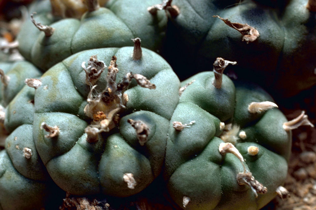
Lophophora williamsii (/loʊˈfɒfərə wɪliˈæmsiaɪ/) or peyote (/pəˈjoʊti/) is a small, spineless cactus with psychoactive alkaloids, particularly mescaline.[2] Peyote is a Spanish word derived from the Nahuatl, or Aztec, peyōtl [ˈpejoːt͡ɬ], meaning "glisten" or "glistening". Other sources translate the Nahuatl word as "Divine Messenger".[3][4] Peyote is native to Mexico and southwestern Texas. It is found primarily in the Sierra Madre Occidental, the Chihuahuan Desert and in the states of Nayarit, Coahuila, Nuevo León, Tamaulipas, and San Luis Potosí among scrub. It flowers from March to May, and sometimes as late as September. The flowers are pink, with thigmotactic anthers (like Opuntia).
Known for its psychoactive properties when ingested, peyote is used worldwide,[citation needed] having a long history of ritualistic and medicinal use by indigenous North Americans. Peyote contains the hallucinogen mescaline.[2]
psylocybiny
Psylocybina (4-PO-DMT) – organiczny związek chemiczny z grupy tryptamin, alkaloid o właściwościach psychodelicznych występujący naturalnie w setkach gatunków grzybów psylocybinowych, m.in. w Psilocybe cubensis i Psilocybe semilanceata. Psylocybina obok LSD jest najbardziej popularnym i najczęściej używanym psychodelikiem. Historia zażywania grzybów psylocybinowych sięga czterech tysięcy lat wstecz, obecnie popularnie znane są one jako halucynogenne lub magiczne grzyby. Psylocybina powoduje głębokie doznania psychodeliczne, transcendentne, mistyczne, medytacyjne, często także religijne.
Obecnie w większości krajów wpisana została na listę nielegalnych środków psychoaktywnych.
Substancja ta została opisana po raz pierwszy w latach 60. XX wieku przez Alberta Hofmanna.
Anhalonium lewinii

Infinite loading is something to consider
+1
Maecenas ultricies mi eget mauris pharetra.
To zupełnie nie tak!
Ornare arcu dui vivamus arcu felis bibendum ut.
This article is for demo purposes only.
Mauris
Who?
IPFS
Never Heard of it
notification
Where?
This is an attempt to answer the basic question of human existence
Far reaching words
Could IFPS solve the problem of Hypothes.is orphaning the links after slug changes?
Test
Test
facts
How does one ensure a fact?
post
That can be commented on like this.
This is a prototype of new engine
fuel
ty
Activity Streams Fuel.Press/YOURNAME
fuel press
Right here! You can annotate every single word/paragraph too! Just select the text and join the conversation.
For all other except clauses - which really should be the vast majority - the caught exception type must be as specific as possible. Something like KeyError, or ConnectionTimeout, etc.
!
Under the mainstream physicalist view that brain activity is, or somehow generates, the mind, the findings certainly seem counterintuitive: How can the richness of experience go up when brain activity goes down? Understandably, therefore, researchers have subsequently endeavored to find something in patterns of brain activity that reliably increases in psychedelic states. Alternatives include brain activity variability, functional coupling between different brain areas and, most recently, a property of brain activity variously labeled as "complexity," "diversity," "entropy" or "randomness" - terms viewed as approximately synonymous.
Important, it seems.
Cancer patients often develop chronic, clinically significant symptoms of depression and anxiety. Previous studies suggest that psilocybin may decrease depression and anxiety in cancer patients. The effects of psilocybin were studied in 51 cancer patients with life-threatening diagnoses and symptoms of depression and/or anxiety. This randomized, double-blind, cross-over trial investigated the effects of a very low (placebo-like) dose (1 or 3 mg/70 kg) vs. a high dose (22 or 30 mg/70 kg) of psilocybin administered in counterbalanced sequence with 5 weeks between sessions and a 6-month follow-up. Instructions to participants and staff minimized expectancy effects. Participants, staff, and community observers rated participant moods, attitudes, and behaviors throughout the study. High-dose psilocybin produced large decreases in clinician- and self-rated measures of depressed mood and anxiety, along with increases in quality of life, life meaning, and optimism, and decreases in death anxiety. At 6-month follow-up, these changes were sustained, with about 80% of participants continuing to show clinically significant decreases in depressed mood and anxiety. Participants attributed improvements in attitudes about life/self, mood, relationships, and spirituality to the high-dose experience, with >80% endorsing moderately or greater increased well-being/life satisfaction. Community observer ratings showed corresponding changes. Mystical-type psilocybin experience on session day mediated the effect of psilocybin dose on therapeutic outcomes.
Abstract
To be continued.
When?
annotation
Right here! You can annotate every single word/paragraph too! Just select the text and join the conversation.
neurogroove.info
Polish repository of 'trip raports'. It is heavily moderated, user is permitted to provide details about their substance, dosage, previous experience, set & setting and age. All the above makes NG a valid source for testing the hypothesis.
mystical experience
Mysticism scaleThis 32-item questionnaire was developed to assess primary mystical experiences (Hood et al.2001;Spilka et al.2005).
The Mysticism Scale has been exten-sively studied, demonstrates cross-cultural generalizability,and is well regarded in the field of the psychology ofreligion (Hood et al.2001; Spilka et al.2005) but has notpreviously been used to assess changes after a drug experience.
A total score and three empirically derived factors aremeasured: interpretation (corresponding to three mysticaldimensions described by Stace (1960): noetic quality,deeply felt positive mood, and sacredness); introvertivemysticism (corresponding to the Stace dimensions ofinternal unity, transcendence of time and space, andineffability); and extrovertive mysticism (corresponding tothe dimension of the unity of all things/all things are alive).
The items were rated on a nine-point scale (−4=thisdescription is extremely not true of my own experience orexperiences; 0=I cannot decide; and +4=this description isextremely true of my own experience or experiences). Forthe version of the questionnaire used 7 h after drugadministration, the participants were instructed to completethe questionnaire with reference to their experiences afterthey received the capsules that morning
Psilocybin may induce spiritual experiences in its users.
DOB
Dimethoxybromoamphetamine (DOB), also known as brolamfetamine (INN)[1] and bromo-DMA, is a psychedelic drug and substituted amphetamine of the phenethylamine class of compounds. DOB was first synthesized by Alexander Shulgin in 1967.
Its synthesis and effects are documented in Shulgin's book PiHKAL: A Chemical Love Story.
DOB
Admiral Shulgin
Alexander Theodore Shulgin (June 17, 1925 – June 2, 2014) was an American medicinal chemist, biochemist, organic chemist, pharmacologist, psychopharmacologist, and author. He is credited with introducing MDMA ("ecstasy", "mandy" or "molly") to psychologists in the late 1970s for psychopharmaceutical use and the discovery, synthesis and personal bioassay of over 230 psychoactive compounds for their psychedelic and entactogenic potential.

In 1991 and 1997, he and his wife Ann Shulgin compiled the books PIHKAL and TIHKAL (standing for Phenethylamines and Tryptamines I Have Known And Loved), from notebooks which extensively described their work and personal experiences with these two classes of psychoactive drugs. Shulgin performed seminal work into the descriptive synthesis of many of these compounds. Some of Shulgin's noteworthy discoveries include compounds of the 2C* family (such as 2C-B) and compounds of the DOx family (such as DOM).
Due in part to Shulgin's extensive work in the field of psychedelic research and the rational drug design of psychedelic drugs, he has since been dubbed the "godfather of psychedelics".
recruiting volunteers
If you feel like participating leave a comment in this thread.
It also means recognizing that our civic infrastructure was built for the normative perpetuation of a status quo that is morally wrong and fundamentally unsustainable. As a society, we don’t need to agree on policy choice, problem framing, or ideology. But can we agree to build the infrastructure needed to have those conversations? Can we move toward centering different stories?
Make no mistake: this isn’t a technology issue, but a civil rights issue. Unfortunately, there’s a lot of jargon (technical terminology, marketing hype, legalese), keeping communities from engaging in the wave of data collection and technology procurement that will shape how social services like education, welfare, and child protection are delivered for decades to come. There’s little space for the meaningful and collaborative radical reimagining of alternative futures when the public is repeatedly told that the revolution is already here and they just don’t understand it.
“Roadside Picnic” by Arkady Strugatsky
Roadside Picnic (Russian: Пикник на обочине, Piknik na obochine, IPA: [pʲɪkˈnʲik nɐ ɐˈbotɕɪnʲe]) is a science fiction novel by Soviet-Russian authors Arkady and Boris Strugatsky, written in 1971 and published in 1972. The story leads among other works of the authors on the number of translations into foreign languages and publications outside the former Soviet Union. As of 2003, Boris Strugatsky has counted 55 publications of "Picnic" in 22 countries.
The story is published in English in a translation by Antonina W. Bouis. A preface to the first American edition (MacMillan Publishing Co., Inc., New York, 1977) was written by Theodore Sturgeon. Stanislaw Lem wrote an afterword to the German edition of 1977.
The term "stalker" became a part of the Russian language and, according to the authors, became the most popular of their neologisms. In the context of the book, a stalker is a person who breaks the prohibitions, enters the Zone and takes out various artifacts from it, which he then usually sells and thereby earns a living. In Russian, after Tarkovsky's film, this term acquired the meaning of a guide who navigates in various forbidden and uncharted territories; later on, fans of industrial tourism, especially those visiting abandoned sites and ghost towns, were also called stalkers.
The 1979 film Stalker, directed by Andrei Tarkovsky, is loosely based on the novel, with a screenplay written by the Strugatsky brothers.

Stalker (1979)
Wchodziło długo, prawdziwie odurzony byłem po godzinie. Stan, w którym się znalazłem można określić jednym słowem, ale pisanym koniecznie z wielkiej litery: Spokój. Wielki Spokój, jakby nic złego nigdy się nie działo, jakby moje wnętrze było boską harmonią, idealnie zestrojoną z zachwycającym światem wokół. Myślałem i mówiłem bardzo trzeźwo: być może tak trzeźwo, jak nigdy: wyzbyty bowiem byłem z najmniejszych śladów niepewności, wstydu, nerwów, kompleksów... Było tak, jakbym znalazł w umyśle właściwe drzwiczki, tej najwygodniejszy pokój i rozłożył się w nim, delektując się (w nienarcystyczny sposób) sobą, swoim byciem i byciem, które mnie otaczało: świata, przedmiotów, światła, ludzi, Krzyśka, Andrzeja. Wszystko było dobre, a jeśli nie było - nie było godne uwagi. Zdumiewała mnie refleksja nad idiotyzmem wielkiej części moich codziennych zmartwień, wszystkich tych mniejszych i większych narcyzmów, skupienia na naskórku rzeczywistości. Andrzej w międzyczasie znalazł się w bardzo podobnym stanie, tylko, że połączonym z OEVami (opened eyes' visuals), do tego mówił dużo, gestykulując i intonując jak dziecko: "Przecież to wszystko takie proste...! Takie proste! A ludzie się przejmują!".
Mystical experience description detected.
Fajny TR, świetnie oddaje klimat pierwszego zetknięcia się z grzybami. Przypomina mi trochę moje początki; pierwszy trip był w 100% pozytywny, drugi to właśnie bad trip na tych samych zasadach, co u ciebie (zobaczenie siebie i swojego życia w boleśnie negatywnym świetle).
Hypothesis: Badtrip content is not random. Usually very personal.
Dresiarskie towarzystwo siedziało w cieniu, słyszałem niekoniecznie kulturalną rozmowę. Nie czułem wobec nich niczego negatywnego; co najwyżej współczułem prostackiej egzystencji. Na klepisku pośrodku podwórza, rzucając długie cienie, bawił się chłopiec z dużym psem, chyba owczarkiem niemieckim. Rzucał mu piłkę, klepał radośnie po tułowiu, pies się na niego rzucał, chłopiec robił uniki, śmiejąc się... Każdemu ruchowi, każdej konfiguracji towarzyszyło wydłużone, konturowe odbicie na ziemi. Nie mogłem oderwać oczu, oczarowany widowiskiem. Jak dzisiaj o tym myślę - miałem szczęście, bo widok ten uważam za wyjątkowy niezależnie, czy jestem pod wpływem, czy nie.
<3
Zdaniem psychiatrów taki stan odurzenia może być wyjątkowo niebezpieczny.
Can mushrooms be dangerous? Yes. Are mushrooms extremely dangerous as stated in this paragraph? Likely not. Source:

Wallets: This feature allows you to receive, store and spend our currency – Bit.Fuel – as well as Ethereum or any ERC-20 compatible token/coin. After a while, when you gather some fuel, you will be able to spend it on (not so) microjobs that we offer, like Website Development & implementation, courses that we will launch in the near future or everything available at our shop.
let's talk!
This publication is work in progress.
You can track changes in this thread.
Psilocybin can occasion mystical-type experienceshaving substantial and sustained personalmeaning and spiritual significance
Hypothesis.
Guy Fawkes masks

SNAFU
What does it mean?
Admiral Shulgin
Alexander Theodore Shulgin (June 17, 1925 – June 2, 2014) was an American medicinal chemist, biochemist, organic chemist, pharmacologist, psychopharmacologist, and author. He is credited with introducing MDMA ("ecstasy", "mandy" or "molly") to psychologists in the late 1970s for psychopharmaceutical use and for the discovery, synthesis and personal bioassay of over 230 psychoactive compounds for their psychedelic and entactogenic potential.
In 1991 and 1997, he and his wife Ann Shulgin compiled the books PIHKAL and TIHKAL (standing for Phenethylamines and Tryptamines I Have Known And Loved), from notebooks which extensively described their work and personal experiences with these two classes of psychoactive drugs. Shulgin performed seminal work into the descriptive synthesis of many of these compounds. Some of Shulgin's noteworthy discoveries include compounds of the 2C* family (such as 2C-B) and compounds of the DOx family (such as DOM).
Due in part to Shulgin's extensive work in the field of psychedelic research and the rational drug design of psychedelic drugs, he has since been dubbed the "godfather of psychedelics".
You are curious why we don’t hide our faces. Have you ever heard the story of Uncatchable Joe?
Two cowboys, a newcomer and an old-timer, are drinking beer in front of a saloon. Suddenly, there is a clatter of hooves, a great cloud of dust, and something moving extremely fast from one end of town to the other. The newcomer looks at the old-timer, but seeing no reaction, decides to let the matter drop. However, several minutes later, the same cloud of dust, accompanied by the clatter of hooves, rapidly proceeds in the other direction. Not being able to see what’s behind the dust, and unable to contain his curiosity any longer, the newcomer asks: “OK, what the hell was that, Bill?” / “Oh, that’s Uncatchable Joe. Nobody has ever managed to catch him, Harry.” / “Why? Is he so fast, Bill?” / “Nope, it’s just because nobody needs him, Harry.”
Source: https://medium.com/@EwardEd/the-uncatchable-joe-or-a-life-that-you-want-5825068beabc
buy
Change to get
reward
You van exchange IT for services here at fuel.press
Could I find a Freelancer who can get it done?
halucynogenne
Nieprawdą jest, że psylocybina powoduje halucynacje.
Efekty wizualne wywoływane przez psychodeliki nie polegają na widzeniu urojonych obiektów, lecz na widzeniu w obiektach rzeczywistych czegoś, czym nie są – np. drzewo może wydawać się człowiekiem, kształty i kolory mogą ulegać deformacjom, może zaniknąć poczucie skali – coś, co jest małe, może być postrzegane jako wielkie, czas może się rozciągać bądź zagęszczać.
Psylocybina
Psylocybina (4-PO-DMT) – organiczny związek chemiczny z grupy tryptamin, alkaloid o właściwościach psychodelicznych występujący naturalnie w setkach gatunków grzybów psylocybinowych, m.in. w Psilocybe cubensis i Psilocybe semilanceata. Psylocybina obok LSD jest najbardziej popularnym i najczęściej używanym psychodelikiem. Historia zażywania grzybów psylocybinowych sięga czterech tysięcy lat wstecz, obecnie popularnie znane są one jako halucynogenne lub magiczne grzyby. Psylocybina powoduje głębokie doznania psychodeliczne, transcendentne, mistyczne, medytacyjne, często także religijne.
Obecnie w większości krajów wpisana została na listę nielegalnych środków psychoaktywnych.
Substancja ta została opisana po raz pierwszy w latach 60. XX wieku przez Alberta Hofmanna.
Docs
Great example: 
Survey completion used for scientific research
I frequently talk with people who are not that concerned about surveillance, or who feel that the positives outweigh the risks. Here, I want to share some important truths about surveillance: Surveillance can facilitate human rights abuses and even genocide Data is often used for different purposes than why it was collected Data often contains errors Surveillance typically operates with no accountability Surveillance changes our behavior Surveillance disproportionately impacts the marginalized Data privacy is a public good We don’t have to accept invasive surveillance
As a prototype it hits a sweet spot: it's challenging - it's no small feat to recognize handwritten digits - but it's not so difficult as to require an extremely complicated solution, or tremendous computational power. Furthermore, it's a great way to develop more advanced techniques, such as deep learning. And so throughout the book we'll return repeatedly to the problem of handwriting recognition. Later in the book, we'll discuss how these ideas may be applied to other problems in computer vision, and also in speech, natural language processing, and other domains.Of course, if the point of the chapter was only to write a computer program to recognize handwritten digits, then the chapter would be much shorter! But along the way we'll develop many key ideas about neural networks, including two important types of artificial neuron (the perceptron and the sigmoid neuron), and the standard learning algorithm for neural networks, known as stochastic gradient descent. Throughout, I focus on explaining why things are done the way they are, and on building your neural networks intuition. That requires a lengthier discussion than if I just presented the basic mechanics of what's going on, but it's worth it for the deeper understanding you'll attain. Amongst the payoffs, by the end of the chapter we'll be in position to understand what deep learning is, and why it matters.PerceptronsWhat is a neural network? To get started, I'll explain a type of artificial neuron called a perceptron. Perceptrons were developed in the 1950s and 1960s by the scientist Frank Rosenblatt, inspired by earlier work by Warren McCulloch and Walter Pitts. Today, it's more common to use other models of artificial neurons - in this book, and in much modern work on neural networks, the main neuron model used is one called the sigmoid neuron. We'll get to sigmoid neurons shortly. But to understand why sigmoid neurons are defined the way they are, it's worth taking the time to first understand perceptrons.So how do perceptrons work? A perceptron takes several binary inputs, x1,x2,…x1,x2,…x_1, x_2, \ldots, and produces a single binary output: In the example shown the perceptron has three inputs, x1,x2,x3x1,x2,x3x_1, x_2, x_3. In general it could have more or fewer inputs. Rosenblatt proposed a simple rule to compute the output. He introduced weights, w1,w2,…w1,w2,…w_1,w_2,\ldots, real numbers expressing the importance of the respective inputs to the output. The neuron's output, 000 or 111, is determined by whether the weighted sum ∑jwjxj∑jwjxj\sum_j w_j x_j is less than or greater than some threshold value. Just like the weights, the threshold is a real number which is a parameter of the neuron. To put it in more precise algebraic terms: output={01if ∑jwjxj≤ thresholdif ∑jwjxj> threshold(1)(1)output={0if ∑jwjxj≤ threshold1if ∑jwjxj> threshold\begin{eqnarray} \mbox{output} & = & \left\{ \begin{array}{ll} 0 & \mbox{if } \sum_j w_j x_j \leq \mbox{ threshold} \\ 1 & \mbox{if } \sum_j w_j x_j > \mbox{ threshold} \end{array} \right. \tag{1}\end{eqnarray} That's all there is to how a perceptron works!That's the basic mathematical model. A way you can think about the perceptron is that it's a device that makes decisions by weighing up evidence. Let me give an example. It's not a very realistic example, but it's easy to understand, and we'll soon get to more realistic examples. Suppose the weekend is coming up, and you've heard that there's going to be a cheese festival in your city. You like cheese, and are trying to decide whether or not to go to the festival. You might make your decision by weighing up three factors: Is the weather good? Does your boyfriend or girlfriend want to accompany you? Is the festival near public transit? (You don't own a car). We can represent these three factors by corresponding binary variables x1,x2x1,x2x_1, x_2, and x3x3x_3. For instance, we'd have x1=1x1=1x_1 = 1 if the weather is good, and x1=0x1=0x_1 = 0 if the weather is bad. Similarly, x2=1x2=1x_2 = 1 if your boyfriend or girlfriend wants to go, and x2=0x2=0x_2 = 0 if not. And similarly again for x3x3x_3 and public transit.Now, suppose you absolutely adore cheese, so much so that you're happy to go to the festival even if your boyfriend or girlfriend is uninterested and the festival is hard to get to. But perhaps you really loathe bad weather, and there's no way you'd go to the festival if the weather is bad. You can use perceptrons to model this kind of decision-making. One way to do this is to choose a weight w1=6w1=6w_1 = 6 for the weather, and w2=2w2=2w_2 = 2 and w3=2w3=2w_3 = 2 for the other conditions. The larger value of w1w1w_1 indicates that the weather matters a lot to you, much more than whether your boyfriend or girlfriend joins you, or the nearness of public transit. Finally, suppose you choose a threshold of 555 for the perceptron. With these choices, the perceptron implements the desired decision-making model, outputting 111 whenever the weather is good, and 000 whenever the weather is bad. It makes no difference to the output whether your boyfriend or girlfriend wants to go, or whether public transit is nearby.By varying the weights and the threshold, we can get different models of decision-making. For example, suppose we instead chose a threshold of 333. Then the perceptron would decide that you should go to the festival whenever the weather was good or when both the festival was near public transit and your boyfriend or girlfriend was willing to join you. In other words, it'd be a different model of decision-making. Dropping the threshold means you're more willing to go to the festival.Obviously, the perceptron isn't a complete model of human decision-making! But what the example illustrates is how a perceptron can weigh up different kinds of evidence in order to make decisions. And it should seem plausible that a complex network of perceptrons could make quite subtle decisions: In this network, the first column of perceptrons - what we'll call the first layer of perceptrons - is making three very simple decisions, by weighing the input evidence. What about the perceptrons in the second layer? Each of those perceptrons is making a decision by weighing up the results from the first layer of decision-making. In this way a perceptron in the second layer can make a decision at a more complex and more abstract level than perceptrons in the first layer. And even more complex decisions can be made by the perceptron in the third layer. In this way, a many-layer network of perceptrons can engage in sophisticated decision making.Incidentally, when I defined perceptrons I said that a perceptron has just a single output. In the network above the perceptrons look like they have multiple outputs. In fact, they're still single output. The multiple output arrows are merely a useful way of indicating that the output from a perceptron is being used as the input to several other perceptrons. It's less unwieldy than drawing a single output line which then splits.Let's simplify the way we describe perceptrons. The condition ∑jwjxj>threshold∑jwjxj>threshold\sum_j w_j x_j > \mbox{threshold} is cumbersome, and we can make two notational changes to simplify it. The first change is to write ∑jwjxj∑jwjxj\sum_j w_j x_j as a dot product, w⋅x≡∑jwjxjw⋅x≡∑jwjxjw \cdot x \equiv \sum_j w_j x_j, where www and xxx are vectors whose components are the weights and inputs, respectively. The second change is to move the threshold to the other side of the inequality, and to replace it by what's known as the perceptron's bias, b≡−thresholdb≡−thresholdb \equiv -\mbox{threshold}. Using the bias instead of the threshold, the perceptron rule can be rewritten: output={01if w⋅x+b≤0if w⋅x+b>0(2)(2)output={0if w⋅x+b≤01if w⋅x+b>0\begin{eqnarray} \mbox{output} = \left\{ \begin{array}{ll} 0 & \mbox{if } w\cdot x + b \leq 0 \\ 1 & \mbox{if } w\cdot x + b > 0 \end{array} \right. \tag{2}\end{eqnarray} You can think of the bias as a measure of how easy it is to get the perceptron to output a 111. Or to put it in more biological terms, the bias is a measure of how easy it is to get the perceptron to fire. For a perceptron with a really big bias, it's extremely easy for the perceptron to output a 111. But if the bias is very negative, then it's difficult for the perceptron to output a 111. Obviously, introducing the bias is only a small change in how we describe perceptrons, but we'll see later that it leads to further notational simplifications. Because of this, in the remainder of the book we won't use the threshold, we'll always use the bias.I've described perceptrons as a method for weighing evidence to make decisions. Another way perceptrons can be used is to compute the elementary logical functions we usually think of as underlying computation, functions such as AND, OR, and NAND. For example, suppose we have a perceptron with two inputs, each with weight −2−2-2, and an overall bias of 333. Here's our perceptron: Then we see that input 000000 produces output 111, since (−2)∗0+(−2)∗0+3=3(−2)∗0+(−2)∗0+3=3(-2)*0+(-2)*0+3 = 3 is positive. Here, I've introduced the ∗∗* symbol to make the multiplications explicit. Similar calculations show that the inputs 010101 and 101010 produce output 111. But the input 111111 produces output 000, since (−2)∗1+(−2)∗1+3=−1(−2)∗1+(−2)∗1+3=−1(-2)*1+(-2)*1+3 = -1 is negative. And so our perceptron implements a NAND gate!The NAND example shows that we can use perceptrons to compute simple logical functions. In fact, we can use networks of perceptrons to compute any logical function at all. The reason is that the NAND gate is universal for computation, that is, we can build any computation up out of NAND gates. For example, we can use NAND gates to build a circuit which adds two bits, x1x1x_1 and x2x2x_2. This requires computing the bitwise sum, x1⊕x2x1⊕x2x_1 \oplus x_2, as well as a carry bit which is set to 111 when both x1x1x_1 and x2x2x_2 are 111, i.e., the carry bit is just the bitwise product x1x2x1x2x_1 x_2: To get an equivalent network of perceptrons we replace all the NAND gates by perceptrons with two inputs, each with weight −2−2-2, and an overall bias of 333. Here's the resulting network. Note that I've moved the perceptron corresponding to the bottom right NAND gate a little, just to make it easier to draw the arrows on the diagram: One notable aspect of this network of perceptrons is that the output from the leftmost perceptron is used twice as input to the bottommost perceptron. When I defined the perceptron model I didn't say whether this kind of double-output-to-the-same-place was allowed. Actually, it doesn't much matter. If we don't want to allow this kind of thing, then it's possible to simply merge the two lines, into a single connection with a weight of -4 instead of two connections with -2 weights. (If you don't find this obvious, you should stop and prove to yourself that this is equivalent.) With that change, the network looks as follows, with all unmarked weights equal to -2, all biases equal to 3, and a single weight of -4, as marked: Up to now I've been drawing inputs like x1x1x_1 and x2x2x_2 as variables floating to the left of the network of perceptrons. In fact, it's conventional to draw an extra layer of perceptrons - the input layer - to encode the inputs: This notation for input perceptrons, in which we have an output, but no inputs, is a shorthand. It doesn't actually mean a perceptron with no inputs. To see this, suppose we did have a perceptron with no inputs. Then the weighted sum ∑jwjxj∑jwjxj\sum_j w_j x_j would always be zero, and so the perceptron would output 111 if b>0b>0b > 0, and 000 if b≤0b≤0b \leq 0. That is, the perceptron would simply output a fixed value, not the desired value (x1x1x_1, in the example above). It's better to think of the input perceptrons as not really being perceptrons at all, but rather special units which are simply defined to output the desired values, x1,x2,…x1,x2,…x_1, x_2,\ldots.The adder example demonstrates how a network of perceptrons can be used to simulate a circuit containing many NAND gates. And because NAND gates are universal for computation, it follows that perceptrons are also universal for computation.The computational universality of perceptrons is simultaneously reassuring and disappointing. It's reassuring because it tells us that networks of perceptrons can be as powerful as any other computing device. But it's also disappointing, because it makes it seem as though perceptrons are merely a new type of NAND gate. That's hardly big news!However, the situation is better than this view suggests. It turns out that we can devise learning algorithms which can automatically tune the weights and biases of a network of artificial neurons. This tuning happens in response to external stimuli, without direct intervention by a programmer. These learning algorithms enable us to use artificial neurons in a way which is radically different to conventional logic gates. Instead of explicitly laying out a circuit of NAND and other gates, our neural networks can simply learn to solve problems, sometimes problems where it would be extremely difficult to directly design a conventional circuit.Sigmoid neuronsLearning algorithms sound terrific. But how can we devise such algorithms for a neural network? Suppose we have a network of perceptrons that we'd like to use to learn to solve some problem. For example, the inputs to the network might be the raw pixel data from a scanned, handwritten image of a digit. And we'd like the network to learn weights and biases so that the output from the network correctly classifies the digit. To see how learning might work, suppose we make a small change in some weight (or bias) in the network. What we'd like is for this small change in weight to cause only a small corresponding change in the output from the network. As we'll see in a moment, this property will make learning possible. Schematically, here's what we want (obviously this network is too simple to do handwriting recognition!): If it were true that a small change in a weight (or bias) causes only a small change in output, then we could use this fact to modify the weights and biases to get our network to behave more in the manner we want. For example, suppose the network was mistakenly classifying an image as an "8" when it should be a "9". We could figure out how to make a small change in the weights and biases so the network gets a little closer to classifying the image as a "9". And then we'd repeat this, changing the weights and biases over and over to produce better and better output. The network would be learning.The problem is that this isn't what happens when our network contains perceptrons. In fact, a small change in the weights or bias of any single perceptron in the network can sometimes cause the output of that perceptron to completely flip, say from 000 to 111. That flip may then cause the behaviour of the rest of the network to completely change in some very complicated way. So while your "9" might now be classified correctly, the behaviour of the network on all the other images is likely to have completely changed in some hard-to-control way. That makes it difficult to see how to gradually modify the weights and biases so that the network gets closer to the desired behaviour. Perhaps there's some clever way of getting around this problem. But it's not immediately obvious how we can get a network of perceptrons to learn.We can overcome this problem by introducing a new type of artificial neuron called a sigmoid neuron. Sigmoid neurons are similar to perceptrons, but modified so that small changes in their weights and bias cause only a small change in their output. That's the crucial fact which will allow a network of sigmoid neurons to learn.Okay, let me describe the sigmoid neuron. We'll depict sigmoid neurons in the same way we depicted perceptrons: Just like a perceptron, the sigmoid neuron has inputs, x1,x2,…x1,x2,…x_1, x_2, \ldots. But instead of being just 000 or 111, these inputs can also take on any values between 000 and 111. So, for instance, 0.638…0.638…0.638\ldots is a valid input for a sigmoid neuron. Also just like a perceptron, the sigmoid neuron has weights for each input, w1,w2,…w1,w2,…w_1, w_2, \ldots, and an overall bias, bbb. But the output is not 000 or 111. Instead, it's σ(w⋅x+b)σ(w⋅x+b)\sigma(w \cdot x+b), where σσ\sigma is called the sigmoid function* *Incidentally, σσ\sigma is sometimes called the logistic function, and this new class of neurons called logistic neurons. It's useful to remember this terminology, since these terms are used by many people working with neural nets. However, we'll stick with the sigmoid terminology., and is defined by: σ(z)≡11+e−z.(3)(3)σ(z)≡11+e−z.\begin{eqnarray} \sigma(z) \equiv \frac{1}{1+e^{-z}}. \tag{3}\end{eqnarray} To put it all a little more explicitly, the output of a sigmoid neuron with inputs x1,x2,…x1,x2,…x_1,x_2,\ldots, weights w1,w2,…w1,w2,…w_1,w_2,\ldots, and bias bbb is 11+exp(−∑jwjxj−b).(4)(4)11+exp(−∑jwjxj−b).\begin{eqnarray} \frac{1}{1+\exp(-\sum_j w_j x_j-b)}. \tag{4}\end{eqnarray}At first sight, sigmoid neurons appear very different to perceptrons. The algebraic form of the sigmoid function may seem opaque and forbidding if you're not already familiar with it. In fact, there are many similarities between perceptrons and sigmoid neurons, and the algebraic form of the sigmoid function turns out to be more of a technical detail than a true barrier to understanding.To understand the similarity to the perceptron model, suppose z≡w⋅x+bz≡w⋅x+bz \equiv w \cdot x + b is a large positive number. Then e−z≈0e−z≈0e^{-z} \approx 0 and so σ(z)≈1σ(z)≈1\sigma(z) \approx 1. In other words, when z=w⋅x+bz=w⋅x+bz = w \cdot x+b is large and positive, the output from the sigmoid neuron is approximately 111, just as it would have been for a perceptron. Suppose on the other hand that z=w⋅x+bz=w⋅x+bz = w \cdot x+b is very negative. Then e−z→∞e−z→∞e^{-z} \rightarrow \infty, and σ(z)≈0σ(z)≈0\sigma(z) \approx 0. So when z=w⋅x+bz=w⋅x+bz = w \cdot x +b is very negative, the behaviour of a sigmoid neuron also closely approximates a perceptron. It's only when w⋅x+bw⋅x+bw \cdot x+b is of modest size that there's much deviation from the perceptron model.What about the algebraic form of σσ\sigma? How can we understand that? In fact, the exact form of σσ\sigma isn't so important - what really matters is the shape of the function when plotted. Here's the shape: -4-3-2-1012340.00.20.40.60.81.0zsigmoid function function s(x) {return 1/(1+Math.exp(-x));} var m = [40, 120, 50, 120]; var height = 290 - m[0] - m[2]; var width = 600 - m[1] - m[3]; var xmin = -5; var xmax = 5; var sample = 400; var x1 = d3.scale.linear().domain([0, sample]).range([xmin, xmax]); var data = d3.range(sample).map(function(d){ return { x: x1(d), y: s(x1(d))}; }); var x = d3.scale.linear().domain([xmin, xmax]).range([0, width]); var y = d3.scale.linear() .domain([0, 1]) .range([height, 0]); var line = d3.svg.line() .x(function(d) { return x(d.x); }) .y(function(d) { return y(d.y); }) var graph = d3.select("#sigmoid_graph") .append("svg") .attr("width", width + m[1] + m[3]) .attr("height", height + m[0] + m[2]) .append("g") .attr("transform", "translate(" + m[3] + "," + m[0] + ")"); var xAxis = d3.svg.axis() .scale(x) .tickValues(d3.range(-4, 5, 1)) .orient("bottom") graph.append("g") .attr("class", "x axis") .attr("transform", "translate(0, " + height + ")") .call(xAxis); var yAxis = d3.svg.axis() .scale(y) .tickValues(d3.range(0, 1.01, 0.2)) .orient("left") .ticks(5) graph.append("g") .attr("class", "y axis") .call(yAxis); graph.append("path").attr("d", line(data)); graph.append("text") .attr("class", "x label") .attr("text-anchor", "end") .attr("x", width/2) .attr("y", height+35) .text("z"); graph.append("text") .attr("x", (width / 2)) .attr("y", -10) .attr("text-anchor", "middle") .style("font-size", "16px") .text("sigmoid function"); This shape is a smoothed out version of a step function: -4-3-2-1012340.00.20.40.60.81.0zstep function function s(x) {return x < 0 ? 0 : 1;} var m = [40, 120, 50, 120]; var height = 290 - m[0] - m[2]; var width = 600 - m[1] - m[3]; var xmin = -5; var xmax = 5; var sample = 400; var x1 = d3.scale.linear().domain([0, sample]).range([xmin, xmax]); var data = d3.range(sample).map(function(d){ return { x: x1(d), y: s(x1(d))}; }); var x = d3.scale.linear().domain([xmin, xmax]).range([0, width]); var y = d3.scale.linear() .domain([0,1]) .range([height, 0]); var line = d3.svg.line() .x(function(d) { return x(d.x); }) .y(function(d) { return y(d.y); }) var graph = d3.select("#step_graph") .append("svg") .attr("width", width + m[1] + m[3]) .attr("height", height + m[0] + m[2]) .append("g") .attr("transform", "translate(" + m[3] + "," + m[0] + ")"); var xAxis = d3.svg.axis() .scale(x) .tickValues(d3.range(-4, 5, 1)) .orient("bottom") graph.append("g") .attr("class", "x axis") .attr("transform", "translate(0, " + height + ")") .call(xAxis); var yAxis = d3.svg.axis() .scale(y) .tickValues(d3.range(0, 1.01, 0.2)) .orient("left") .ticks(5) graph.append("g") .attr("class", "y axis") .call(yAxis); graph.append("path").attr("d", line(data)); graph.append("text") .attr("class", "x label") .attr("text-anchor", "end") .attr("x", width/2) .attr("y", height+35) .text("z"); graph.append("text") .attr("x", (width / 2)) .attr("y", -10) .attr("text-anchor", "middle") .style("font-size", "16px") .text("step function"); If σσ\sigma had in fact been a step function, then the sigmoid neuron would be a perceptron, since the output would be 111 or 000 depending on whether w⋅x+bw⋅x+bw\cdot x+b was positive or negative* *Actually, when w⋅x+b=0w⋅x+b=0w \cdot x +b = 0 the perceptron outputs 000, while the step function outputs 111. So, strictly speaking, we'd need to modify the step function at that one point. But you get the idea.. By using the actual σσ\sigma function we get, as already implied above, a smoothed out perceptron. Indeed, it's the smoothness of the σσ\sigma function that is the crucial fact, not its detailed form. The smoothness of σσ\sigma means that small changes ΔwjΔwj\Delta w_j in the weights and ΔbΔb\Delta b in the bias will produce a small change ΔoutputΔoutput\Delta \mbox{output} in the output from the neuron. In fact, calculus tells us that ΔoutputΔoutput\Delta \mbox{output} is well approximated by Δoutput≈∑j∂output∂wjΔwj+∂output∂bΔb,(5)(5)Δoutput≈∑j∂output∂wjΔwj+∂output∂bΔb,\begin{eqnarray} \Delta \mbox{output} \approx \sum_j \frac{\partial \, \mbox{output}}{\partial w_j} \Delta w_j + \frac{\partial \, \mbox{output}}{\partial b} \Delta b, \tag{5}\end{eqnarray} where the sum is over all the weights, wjwjw_j, and ∂output/∂wj∂output/∂wj\partial \, \mbox{output} / \partial w_j and ∂output/∂b∂output/∂b\partial \, \mbox{output} /\partial b denote partial derivatives of the outputoutput\mbox{output} with respect to wjwjw_j and bbb, respectively. Don't panic if you're not comfortable with partial derivatives! While the expression above looks complicated, with all the partial derivatives, it's actually saying something very simple (and which is very good news): ΔoutputΔoutput\Delta \mbox{output} is a linear function of the changes ΔwjΔwj\Delta w_j and ΔbΔb\Delta b in the weights and bias. This linearity makes it easy to choose small changes in the weights and biases to achieve any desired small change in the output. So while sigmoid neurons have much of the same qualitative behaviour as perceptrons, they make it much easier to figure out how changing the weights and biases will change the output.If it's the shape of σσ\sigma which really matters, and not its exact form, then why use the particular form used for σσ\sigma in Equation (3)σ(z)≡11+e−zσ(z)≡11+e−z\begin{eqnarray} \sigma(z) \equiv \frac{1}{1+e^{-z}} \nonumber\end{eqnarray}$('#margin_387419264610_reveal').click(function() {$('#margin_387419264610').toggle('slow', function() {});});? In fact, later in the book we will occasionally consider neurons where the output is f(w⋅x+b)f(w⋅x+b)f(w \cdot x + b) for some other activation function f(⋅)f(⋅)f(\cdot). The main thing that changes when we use a different activation function is that the particular values for the partial derivatives in Equation (5)Δoutput≈∑j∂output∂wjΔwj+∂output∂bΔbΔoutput≈∑j∂output∂wjΔwj+∂output∂bΔb\begin{eqnarray} \Delta \mbox{output} \approx \sum_j \frac{\partial \, \mbox{output}}{\partial w_j} \Delta w_j + \frac{\partial \, \mbox{output}}{\partial b} \Delta b \nonumber\end{eqnarray}$('#margin_727997094331_reveal').click(function() {$('#margin_727997094331').toggle('slow', function() {});}); change. It turns out that when we compute those partial derivatives later, using σσ\sigma will simplify the algebra, simply because exponentials have lovely properties when differentiated. In any case, σσ\sigma is commonly-used in work on neural nets, and is the activation function we'll use most often in this book.How should we interpret the output from a sigmoid neuron? Obviously, one big difference between perceptrons and sigmoid neurons is that sigmoid neurons don't just output 000 or 111. They can have as output any real number between 000 and 111, so values such as 0.173…0.173…0.173\ldots and 0.689…0.689…0.689\ldots are legitimate outputs. This can be useful, for example, if we want to use the output value to represent the average intensity of the pixels in an image input to a neural network. But sometimes it can be a nuisance. Suppose we want the output from the network to indicate either "the input image is a 9" or "the input image is not a 9". Obviously, it'd be easiest to do this if the output was a 000 or a 111, as in a perceptron. But in practice we can set up a convention to deal with this, for example, by deciding to interpret any output of at least 0.50.50.5 as indicating a "9", and any output less than 0.50.50.5 as indicating "not a 9". I'll always explicitly state when we're using such a convention, so it shouldn't cause any confusion. Exercises Sigmoid neurons simulating perceptrons, part I \mbox{} Suppose we take all the weights and biases in a network of perceptrons, and multiply them by a positive constant, c>0c>0c > 0. Show that the behaviour of the network doesn't change.Sigmoid neurons simulating perceptrons, part II \mbox{} Suppose we have the same setup as the last problem - a network of perceptrons. Suppose also that the overall input to the network of perceptrons has been chosen. We won't need the actual input value, we just need the input to have been fixed. Suppose the weights and biases are such that w⋅x+b≠0w⋅x+b≠0w \cdot x + b \neq 0 for the input xxx to any particular perceptron in the network. Now replace all the perceptrons in the network by sigmoid neurons, and multiply the weights and biases by a positive constant c>0c>0c > 0. Show that in the limit as c→∞c→∞c \rightarrow \infty the behaviour of this network of sigmoid neurons is exactly the same as the network of perceptrons. How can this fail when w⋅x+b=0w⋅x+b=0w \cdot x + b = 0 for one of the perceptrons? The architecture of neural networksIn the next section I'll introduce a neural network that can do a pretty good job classifying handwritten digits. In preparation for that, it helps to explain some terminology that lets us name different parts of a network. Suppose we have the network: As mentioned earlier, the leftmost layer in this network is called the input layer, and the neurons within the layer are called input neurons. The rightmost or output layer contains the output neurons, or, as in this case, a single output neuron. The middle layer is called a hidden layer, since the neurons in this layer are neither inputs nor outputs. The term "hidden" perhaps sounds a little mysterious - the first time I heard the term I thought it must have some deep philosophical or mathematical significance - but it really means nothing more than "not an input or an output". The network above has just a single hidden layer, but some networks have multiple hidden layers. For example, the following four-layer network has two hidden layers: Somewhat confusingly, and for historical reasons, such multiple layer networks are sometimes called multilayer perceptrons or MLPs, despite being made up of sigmoid neurons, not perceptrons. I'm not going to use the MLP terminology in this book, since I think it's confusing, but wanted to warn you of its existence.The design of the input and output layers in a network is often straightforward. For example, suppose we're trying to determine whether a handwritten image depicts a "9" or not. A natural way to design the network is to encode the intensities of the image pixels into the input neurons. If the image is a 646464 by 646464 greyscale image, then we'd have 4,096=64×644,096=64×644,096 = 64 \times 64 input neurons, with the intensities scaled appropriately between 000 and 111. The output layer will contain just a single neuron, with output values of less than 0.50.50.5 indicating "input image is not a 9", and values greater than 0.50.50.5 indicating "input image is a 9 ". While the design of the input and output layers of a neural network is often straightforward, there can be quite an art to the design of the hidden layers. In particular, it's not possible to sum up the design process for the hidden layers with a few simple rules of thumb. Instead, neural networks researchers have developed many design heuristics for the hidden layers, which help people get the behaviour they want out of their nets. For example, such heuristics can be used to help determine how to trade off the number of hidden layers against the time required to train the network. We'll meet several such design heuristics later in this book. Up to now, we've been discussing neural networks where the output from one layer is used as input to the next layer. Such networks are called feedforward neural networks. This means there are no loops in the network - information is always fed forward, never fed back. If we did have loops, we'd end up with situations where the input to the σσ\sigma function depended on the output. That'd be hard to make sense of, and so we don't allow such loops.However, there are other models of artificial neural networks in which feedback loops are possible. These models are called recurrent neural networks. The idea in these models is to have neurons which fire for some limited duration of time, before becoming quiescent. That firing can stimulate other neurons, which may fire a little while later, also for a limited duration. That causes still more neurons to fire, and so over time we get a cascade of neurons firing. Loops don't cause problems in such a model, since a neuron's output only affects its input at some later time, not instantaneously.Recurrent neural nets have been less influential than feedforward networks, in part because the learning algorithms for recurrent nets are (at least to date) less powerful. But recurrent networks are still extremely interesting. They're much closer in spirit to how our brains work than feedforward networks. And it's possible that recurrent networks can solve important problems which can only be solved with great difficulty by feedforward networks. However, to limit our scope, in this book we're going to concentrate on the more widely-used feedforward networks.A simple network to classify handwritten digitsHaving defined neural networks, let's return to handwriting recognition. We can split the problem of recognizing handwritten digits into two sub-problems. First, we'd like a way of breaking an image containing many digits into a sequence of separate images, each containing a single digit. For example, we'd like to break the imageinto six separate images, We humans solve this segmentation problem with ease, but it's challenging for a computer program to correctly break up the image. Once the image has been segmented, the program then needs to classify each individual digit. So, for instance, we'd like our program to recognize that the first digit above,is a 5.We'll focus on writing a program to solve the second problem, that is, classifying individual digits. We do this because it turns out that the segmentation problem is not so difficult to solve, once you have a good way of classifying individual digits. There are many approaches to solving the segmentation problem. One approach is to trial many different ways of segmenting the image, using the individual digit classifier to score each trial segmentation. A trial segmentation gets a high score if the individual digit classifier is confident of its classification in all segments, and a low score if the classifier is having a lot of trouble in one or more segments. The idea is that if the classifier is having trouble somewhere, then it's probably having trouble because the segmentation has been chosen incorrectly. This idea and other variations can be used to solve the segmentation problem quite well. So instead of worrying about segmentation we'll concentrate on developing a neural network which can solve the more interesting and difficult problem, namely, recognizing individual handwritten digits.To recognize individual digits we will use a three-layer neural network: The input layer of the network contains neurons encoding the values of the input pixels. As discussed in the next section, our training data for the network will consist of many 282828 by 282828 pixel images of scanned handwritten digits, and so the input layer contains 784=28×28784=28×28784 = 28 \times 28 neurons. For simplicity I've omitted most of the 784784784 input neurons in the diagram above. The input pixels are greyscale, with a value of 0.00.00.0 representing white, a value of 1.01.01.0 representing black, and in between values representing gradually darkening shades of grey.The second layer of the network is a hidden layer. We denote the number of neurons in this hidden layer by nnn, and we'll experiment with different values for nnn. The example shown illustrates a small hidden layer, containing just n=15n=15n = 15 neurons.The output layer of the network contains 10 neurons. If the first neuron fires, i.e., has an output ≈1≈1\approx 1, then that will indicate that the network thinks the digit is a 000. If the second neuron fires then that will indicate that the network thinks the digit is a 111. And so on. A little more precisely, we number the output neurons from 000 through 999, and figure out which neuron has the highest activation value. If that neuron is, say, neuron number 666, then our network will guess that the input digit was a 666. And so on for the other output neurons.You might wonder why we use 101010 output neurons. After all, the goal of the network is to tell us which digit (0,1,2,…,90,1,2,…,90, 1, 2, \ldots, 9) corresponds to the input image. A seemingly natural way of doing that is to use just 444 output neurons, treating each neuron as taking on a binary value, depending on whether the neuron's output is closer to 000 or to 111. Four neurons are enough to encode the answer, since 24=1624=162^4 = 16 is more than the 10 possible values for the input digit. Why should our network use 101010 neurons instead? Isn't that inefficient? The ultimate justification is empirical: we can try out both network designs, and it turns out that, for this particular problem, the network with 101010 output neurons learns to recognize digits better than the network with 444 output neurons. But that leaves us wondering why using 101010 output neurons works better. Is there some heuristic that would tell us in advance that we should use the 101010-output encoding instead of the 444-output encoding?To understand why we do this, it helps to think about what the neural network is doing from first principles. Consider first the case where we use 101010 output neurons. Let's concentrate on the first output neuron, the one that's trying to decide whether or not the digit is a 000. It does this by weighing up evidence from the hidden layer of neurons. What are those hidden neurons doing? Well, just suppose for the sake of argument that the first neuron in the hidden layer detects whether or not an image like the following is present:It can do this by heavily weighting input pixels which overlap with the image, and only lightly weighting the other inputs. In a similar way, let's suppose for the sake of argument that the second, third, and fourth neurons in the hidden layer detect whether or not the following images are present:As you may have guessed, these four images together make up the 000 image that we saw in the line of digits shown earlier:So if all four of these hidden neurons are firing then we can conclude that the digit is a 000. Of course, that's not the only sort of evidence we can use to conclude that the image was a 000 - we could legitimately get a 000 in many other ways (say, through translations of the above images, or slight distortions). But it seems safe to say that at least in this case we'd conclude that the input was a 000.Supposing the neural network functions in this way, we can give a plausible explanation for why it's better to have 101010 outputs from the network, rather than 444. If we had 444 outputs, then the first output neuron would be trying to decide what the most significant bit of the digit was. And there's no easy way to relate that most significant bit to simple shapes like those shown above. It's hard to imagine that there's any good historical reason the component shapes of the digit will be closely related to (say) the most significant bit in the output.Now, with all that said, this is all just a heuristic. Nothing says that the three-layer neural network has to operate in the way I described, with the hidden neurons detecting simple component shapes. Maybe a clever learning algorithm will find some assignment of weights that lets us use only 444 output neurons. But as a heuristic the way of thinking I've described works pretty well, and can save you a lot of time in designing good neural network architectures.Exercise There is a way of determining the bitwise representation of a digit by adding an extra layer to the three-layer network above. The extra layer converts the output from the previous layer into a binary representation, as illustrated in the figure below. Find a set of weights and biases for the new output layer. Assume that the first 333 layers of neurons are such that the correct output in the third layer (i.e., the old output layer) has activation at least 0.990.990.99, and incorrect outputs have activation less than 0.010.010.01. Learning with gradient descentNow that we have a design for our neural network, how can it learn to recognize digits? The first thing we'll need is a data set to learn from - a so-called training data set. We'll use the MNIST data set, which contains tens of thousands of scanned images of handwritten digits, together with their correct classifications. MNIST's name comes from the fact that it is a modified subset of two data sets collected by NIST, the United States' National Institute of Standards and Technology. Here's a few images from MNIST: As you can see, these digits are, in fact, the same as those shown at the beginning of this chapter as a challenge to recognize. Of course, when testing our network we'll ask it to recognize images which aren't in the training set!The MNIST data comes in two parts. The first part contains 60,000 images to be used as training data. These images are scanned handwriting samples from 250 people, half of whom were US Census Bureau employees, and half of whom were high school students. The images are greyscale and 28 by 28 pixels in size. The second part of the MNIST data set is 10,000 images to be used as test data. Again, these are 28 by 28 greyscale images. We'll use the test data to evaluate how well our neural network has learned to recognize digits. To make this a good test of performance, the test data was taken from a different set of 250 people than the original training data (albeit still a group split between Census Bureau employees and high school students). This helps give us confidence that our system can recognize digits from people whose writing it didn't see during training.We'll use the notation xxx to denote a training input. It'll be convenient to regard each training input xxx as a 28×28=78428×28=78428 \times 28 = 784-dimensional vector. Each entry in the vector represents the grey value for a single pixel in the image. We'll denote the corresponding desired output by y=y(x)y=y(x)y = y(x), where yyy is a 101010-dimensional vector. For example, if a particular training image, xxx, depicts a 666, then y(x)=(0,0,0,0,0,0,1,0,0,0)Ty(x)=(0,0,0,0,0,0,1,0,0,0)Ty(x) = (0, 0, 0, 0, 0, 0, 1, 0, 0, 0)^T is the desired output from the network. Note that TTT here is the transpose operation, turning a row vector into an ordinary (column) vector.What we'd like is an algorithm which lets us find weights and biases so that the output from the network approximates y(x)y(x)y(x) for all training inputs xxx. To quantify how well we're achieving this goal we define a cost function* *Sometimes referred to as a loss or objective function. We use the term cost function throughout this book, but you should note the other terminology, since it's often used in research papers and other discussions of neural networks. : C(w,b)≡12n∑x∥y(x)−a∥2.(6)(6)C(w,b)≡12n∑x‖y(x)−a‖2.\begin{eqnarray} C(w,b) \equiv \frac{1}{2n} \sum_x \| y(x) - a\|^2. \tag{6}\end{eqnarray} Here, www denotes the collection of all weights in the network, bbb all the biases, nnn is the total number of training inputs, aaa is the vector of outputs from the network when xxx is input, and the sum is over all training inputs, xxx. Of course, the output aaa depends on xxx, www and bbb, but to keep the notation simple I haven't explicitly indicated this dependence. The notation ∥v∥‖v‖\| v \| just denotes the usual length function for a vector vvv. We'll call CCC the quadratic cost function; it's also sometimes known as the mean squared error or just MSE. Inspecting the form of the quadratic cost function, we see that C(w,b)C(w,b)C(w,b) is non-negative, since every term in the sum is non-negative. Furthermore, the cost C(w,b)C(w,b)C(w,b) becomes small, i.e., C(w,b)≈0C(w,b)≈0C(w,b) \approx 0, precisely when y(x)y(x)y(x) is approximately equal to the output, aaa, for all training inputs, xxx. So our training algorithm has done a good job if it can find weights and biases so that C(w,b)≈0C(w,b)≈0C(w,b) \approx 0. By contrast, it's not doing so well when C(w,b)C(w,b)C(w,b) is large - that would mean that y(x)y(x)y(x) is not close to the output aaa for a large number of inputs. So the aim of our training algorithm will be to minimize the cost C(w,b)C(w,b)C(w,b) as a function of the weights and biases. In other words, we want to find a set of weights and biases which make the cost as small as possible. We'll do that using an algorithm known as gradient descent. Why introduce the quadratic cost? After all, aren't we primarily interested in the number of images correctly classified by the network? Why not try to maximize that number directly, rather than minimizing a proxy measure like the quadratic cost? The problem with that is that the number of images correctly classified is not a smooth function of the weights and biases in the network. For the most part, making small changes to the weights and biases won't cause any change at all in the number of training images classified correctly. That makes it difficult to figure out how to change the weights and biases to get improved performance. If we instead use a smooth cost function like the quadratic cost it turns out to be easy to figure out how to make small changes in the weights and biases so as to get an improvement in the cost. That's why we focus first on minimizing the quadratic cost, and only after that will we examine the classification accuracy.Even given that we want to use a smooth cost function, you may still wonder why we choose the quadratic function used in Equation (6)C(w,b)≡12n∑x∥y(x)−a∥2C(w,b)≡12n∑x‖y(x)−a‖2\begin{eqnarray} C(w,b) \equiv \frac{1}{2n} \sum_x \| y(x) - a\|^2 \nonumber\end{eqnarray}$('#margin_501822820305_reveal').click(function() {$('#margin_501822820305').toggle('slow', function() {});});. Isn't this a rather ad hoc choice? Perhaps if we chose a different cost function we'd get a totally different set of minimizing weights and biases? This is a valid concern, and later we'll revisit the cost function, and make some modifications. However, the quadratic cost function of Equation (6)C(w,b)≡12n∑x∥y(x)−a∥2C(w,b)≡12n∑x‖y(x)−a‖2\begin{eqnarray} C(w,b) \equiv \frac{1}{2n} \sum_x \| y(x) - a\|^2 \nonumber\end{eqnarray}$('#margin_555483302348_reveal').click(function() {$('#margin_555483302348').toggle('slow', function() {});}); works perfectly well for understanding the basics of learning in neural networks, so we'll stick with it for now.Recapping, our goal in training a neural network is to find weights and biases which minimize the quadratic cost function C(w,b)C(w,b)C(w, b). This is a well-posed problem, but it's got a lot of distracting structure as currently posed - the interpretation of www and bbb as weights and biases, the σσ\sigma function lurking in the background, the choice of network architecture, MNIST, and so on. It turns out that we can understand a tremendous amount by ignoring most of that structure, and just concentrating on the minimization aspect. So for now we're going to forget all about the specific form of the cost function, the connection to neural networks, and so on. Instead, we're going to imagine that we've simply been given a function of many variables and we want to minimize that function. We're going to develop a technique called gradient descent which can be used to solve such minimization problems. Then we'll come back to the specific function we want to minimize for neural networks.Okay, let's suppose we're trying to minimize some function, C(v)C(v)C(v). This could be any real-valued function of many variables, v=v1,v2,…v=v1,v2,…v = v_1, v_2, \ldots. Note that I've replaced the www and bbb notation by vvv to emphasize that this could be any function - we're not specifically thinking in the neural networks context any more. To minimize C(v)C(v)C(v) it helps to imagine CCC as a function of just two variables, which we'll call v1v1v_1 and v2v2v_2:What we'd like is to find where CCC achieves its global minimum. Now, of course, for the function plotted above, we can eyeball the graph and find the minimum. In that sense, I've perhaps shown slightly too simple a function! A general function, CCC, may be a complicated function of many variables, and it won't usually be possible to just eyeball the graph to find the minimum.One way of attacking the problem is to use calculus to try to find the minimum analytically. We could compute derivatives and then try using them to find places where CCC is an extremum. With some luck that might work when CCC is a function of just one or a few variables. But it'll turn into a nightmare when we have many more variables. And for neural networks we'll often want far more variables - the biggest neural networks have cost functions which depend on billions of weights and biases in an extremely complicated way. Using calculus to minimize that just won't work!(After asserting that we'll gain insight by imagining CCC as a function of just two variables, I've turned around twice in two paragraphs and said, "hey, but what if it's a function of many more than two variables?" Sorry about that. Please believe me when I say that it really does help to imagine CCC as a function of two variables. It just happens that sometimes that picture breaks down, and the last two paragraphs were dealing with such breakdowns. Good thinking about mathematics often involves juggling multiple intuitive pictures, learning when it's appropriate to use each picture, and when it's not.)Okay, so calculus doesn't work. Fortunately, there is a beautiful analogy which suggests an algorithm which works pretty well. We start by thinking of our function as a kind of a valley. If you squint just a little at the plot above, that shouldn't be too hard. And we imagine a ball rolling down the slope of the valley. Our everyday experience tells us that the ball will eventually roll to the bottom of the valley. Perhaps we can use this idea as a way to find a minimum for the function? We'd randomly choose a starting point for an (imaginary) ball, and then simulate the motion of the ball as it rolled down to the bottom of the valley. We could do this simulation simply by computing derivatives (and perhaps some second derivatives) of CCC - those derivatives would tell us everything we need to know about the local "shape" of the valley, and therefore how our ball should roll.Based on what I've just written, you might suppose that we'll be trying to write down Newton's equations of motion for the ball, considering the effects of friction and gravity, and so on. Actually, we're not going to take the ball-rolling analogy quite that seriously - we're devising an algorithm to minimize CCC, not developing an accurate simulation of the laws of physics! The ball's-eye view is meant to stimulate our imagination, not constrain our thinking. So rather than get into all the messy details of physics, let's simply ask ourselves: if we were declared God for a day, and could make up our own laws of physics, dictating to the ball how it should roll, what law or laws of motion could we pick that would make it so the ball always rolled to the bottom of the valley?To make this question more precise, let's think about what happens when we move the ball a small amount Δv1Δv1\Delta v_1 in the v1v1v_1 direction, and a small amount Δv2Δv2\Delta v_2 in the v2v2v_2 direction. Calculus tells us that CCC changes as follows: ΔC≈∂C∂v1Δv1+∂C∂v2Δv2.(7)(7)ΔC≈∂C∂v1Δv1+∂C∂v2Δv2.\begin{eqnarray} \Delta C \approx \frac{\partial C}{\partial v_1} \Delta v_1 + \frac{\partial C}{\partial v_2} \Delta v_2. \tag{7}\end{eqnarray} We're going to find a way of choosing Δv1Δv1\Delta v_1 and Δv2Δv2\Delta v_2 so as to make ΔCΔC\Delta C negative; i.e., we'll choose them so the ball is rolling down into the valley. To figure out how to make such a choice it helps to define ΔvΔv\Delta v to be the vector of changes in vvv, Δv≡(Δv1,Δv2)TΔv≡(Δv1,Δv2)T\Delta v \equiv (\Delta v_1, \Delta v_2)^T, where TTT is again the transpose operation, turning row vectors into column vectors. We'll also define the gradient of CCC to be the vector of partial derivatives, (∂C∂v1,∂C∂v2)T(∂C∂v1,∂C∂v2)T\left(\frac{\partial C}{\partial v_1}, \frac{\partial C}{\partial v_2}\right)^T. We denote the gradient vector by ∇C∇C\nabla C, i.e.: ∇C≡(∂C∂v1,∂C∂v2)T.(8)(8)∇C≡(∂C∂v1,∂C∂v2)T.\begin{eqnarray} \nabla C \equiv \left( \frac{\partial C}{\partial v_1}, \frac{\partial C}{\partial v_2} \right)^T. \tag{8}\end{eqnarray} In a moment we'll rewrite the change ΔCΔC\Delta C in terms of ΔvΔv\Delta v and the gradient, ∇C∇C\nabla C. Before getting to that, though, I want to clarify something that sometimes gets people hung up on the gradient. When meeting the ∇C∇C\nabla C notation for the first time, people sometimes wonder how they should think about the ∇∇\nabla symbol. What, exactly, does ∇∇\nabla mean? In fact, it's perfectly fine to think of ∇C∇C\nabla C as a single mathematical object - the vector defined above - which happens to be written using two symbols. In this point of view, ∇∇\nabla is just a piece of notational flag-waving, telling you "hey, ∇C∇C\nabla C is a gradient vector". There are more advanced points of view where ∇∇\nabla can be viewed as an independent mathematical entity in its own right (for example, as a differential operator), but we won't need such points of view.With these definitions, the expression (7)ΔC≈∂C∂v1Δv1+∂C∂v2Δv2ΔC≈∂C∂v1Δv1+∂C∂v2Δv2\begin{eqnarray} \Delta C \approx \frac{\partial C}{\partial v_1} \Delta v_1 + \frac{\partial C}{\partial v_2} \Delta v_2 \nonumber\end{eqnarray}$('#margin_512380394946_reveal').click(function() {$('#margin_512380394946').toggle('slow', function() {});}); for ΔCΔC\Delta C can be rewritten as ΔC≈∇C⋅Δv.(9)(9)ΔC≈∇C⋅Δv.\begin{eqnarray} \Delta C \approx \nabla C \cdot \Delta v. \tag{9}\end{eqnarray} This equation helps explain why ∇C∇C\nabla C is called the gradient vector: ∇C∇C\nabla C relates changes in vvv to changes in CCC, just as we'd expect something called a gradient to do. But what's really exciting about the equation is that it lets us see how to choose ΔvΔv\Delta v so as to make ΔCΔC\Delta C negative. In particular, suppose we choose Δv=−η∇C,(10)(10)Δv=−η∇C,\begin{eqnarray} \Delta v = -\eta \nabla C, \tag{10}\end{eqnarray} where ηη\eta is a small, positive parameter (known as the learning rate). Then Equation (9)ΔC≈∇C⋅ΔvΔC≈∇C⋅Δv\begin{eqnarray} \Delta C \approx \nabla C \cdot \Delta v \nonumber\end{eqnarray}$('#margin_31741254841_reveal').click(function() {$('#margin_31741254841').toggle('slow', function() {});}); tells us that ΔC≈−η∇C⋅∇C=−η∥∇C∥2ΔC≈−η∇C⋅∇C=−η‖∇C‖2\Delta C \approx -\eta \nabla C \cdot \nabla C = -\eta \|\nabla C\|^2. Because ∥∇C∥2≥0‖∇C‖2≥0\| \nabla C \|^2 \geq 0, this guarantees that ΔC≤0ΔC≤0\Delta C \leq 0, i.e., CCC will always decrease, never increase, if we change vvv according to the prescription in (10)Δv=−η∇CΔv=−η∇C\begin{eqnarray} \Delta v = -\eta \nabla C \nonumber\end{eqnarray}$('#margin_48762573303_reveal').click(function() {$('#margin_48762573303').toggle('slow', function() {});});. (Within, of course, the limits of the approximation in Equation (9)ΔC≈∇C⋅ΔvΔC≈∇C⋅Δv\begin{eqnarray} \Delta C \approx \nabla C \cdot \Delta v \nonumber\end{eqnarray}$('#margin_919658643545_reveal').click(function() {$('#margin_919658643545').toggle('slow', function() {});});). This is exactly the property we wanted! And so we'll take Equation (10)Δv=−η∇CΔv=−η∇C\begin{eqnarray} \Delta v = -\eta \nabla C \nonumber\end{eqnarray}$('#margin_287729255111_reveal').click(function() {$('#margin_287729255111').toggle('slow', function() {});}); to define the "law of motion" for the ball in our gradient descent algorithm. That is, we'll use Equation (10)Δv=−η∇CΔv=−η∇C\begin{eqnarray} \Delta v = -\eta \nabla C \nonumber\end{eqnarray}$('#margin_718723868298_reveal').click(function() {$('#margin_718723868298').toggle('slow', function() {});}); to compute a value for ΔvΔv\Delta v, then move the ball's position vvv by that amount: v→v′=v−η∇C.(11)(11)v→v′=v−η∇C.\begin{eqnarray} v \rightarrow v' = v -\eta \nabla C. \tag{11}\end{eqnarray} Then we'll use this update rule again, to make another move. If we keep doing this, over and over, we'll keep decreasing CCC until - we hope - we reach a global minimum.Summing up, the way the gradient descent algorithm works is to repeatedly compute the gradient ∇C∇C\nabla C, and then to move in the opposite direction, "falling down" the slope of the valley. We can visualize it like this:Notice that with this rule gradient descent doesn't reproduce real physical motion. In real life a ball has momentum, and that momentum may allow it to roll across the slope, or even (momentarily) roll uphill. It's only after the effects of friction set in that the ball is guaranteed to roll down into the valley. By contrast, our rule for choosing ΔvΔv\Delta v just says "go down, right now". That's still a pretty good rule for finding the minimum!To make gradient descent work correctly, we need to choose the learning rate ηη\eta to be small enough that Equation (9)ΔC≈∇C⋅ΔvΔC≈∇C⋅Δv\begin{eqnarray} \Delta C \approx \nabla C \cdot \Delta v \nonumber\end{eqnarray}$('#margin_560455937071_reveal').click(function() {$('#margin_560455937071').toggle('slow', function() {});}); is a good approximation. If we don't, we might end up with ΔC>0ΔC>0\Delta C > 0, which obviously would not be good! At the same time, we don't want ηη\eta to be too small, since that will make the changes ΔvΔv\Delta v tiny, and thus the gradient descent algorithm will work very slowly. In practical implementations, ηη\eta is often varied so that Equation (9)ΔC≈∇C⋅ΔvΔC≈∇C⋅Δv\begin{eqnarray} \Delta C \approx \nabla C \cdot \Delta v \nonumber\end{eqnarray}$('#margin_157848846275_reveal').click(function() {$('#margin_157848846275').toggle('slow', function() {});}); remains a good approximation, but the algorithm isn't too slow. We'll see later how this works. I've explained gradient descent when CCC is a function of just two variables. But, in fact, everything works just as well even when CCC is a function of many more variables. Suppose in particular that CCC is a function of mmm variables, v1,…,vmv1,…,vmv_1,\ldots,v_m. Then the change ΔCΔC\Delta C in CCC produced by a small change Δv=(Δv1,…,Δvm)TΔv=(Δv1,…,Δvm)T\Delta v = (\Delta v_1, \ldots, \Delta v_m)^T is ΔC≈∇C⋅Δv,(12)(12)ΔC≈∇C⋅Δv,\begin{eqnarray} \Delta C \approx \nabla C \cdot \Delta v, \tag{12}\end{eqnarray} where the gradient ∇C∇C\nabla C is the vector ∇C≡(∂C∂v1,…,∂C∂vm)T.(13)(13)∇C≡(∂C∂v1,…,∂C∂vm)T.\begin{eqnarray} \nabla C \equiv \left(\frac{\partial C}{\partial v_1}, \ldots, \frac{\partial C}{\partial v_m}\right)^T. \tag{13}\end{eqnarray} Just as for the two variable case, we can choose Δv=−η∇C,(14)(14)Δv=−η∇C,\begin{eqnarray} \Delta v = -\eta \nabla C, \tag{14}\end{eqnarray} and we're guaranteed that our (approximate) expression (12)ΔC≈∇C⋅ΔvΔC≈∇C⋅Δv\begin{eqnarray} \Delta C \approx \nabla C \cdot \Delta v \nonumber\end{eqnarray}$('#margin_869505431896_reveal').click(function() {$('#margin_869505431896').toggle('slow', function() {});}); for ΔCΔC\Delta C will be negative. This gives us a way of following the gradient to a minimum, even when CCC is a function of many variables, by repeatedly applying the update rule v→v′=v−η∇C.(15)(15)v→v′=v−η∇C.\begin{eqnarray} v \rightarrow v' = v-\eta \nabla C. \tag{15}\end{eqnarray} You can think of this update rule as defining the gradient descent algorithm. It gives us a way of repeatedly changing the position vvv in order to find a minimum of the function CCC. The rule doesn't always work - several things can go wrong and prevent gradient descent from finding the global minimum of CCC, a point we'll return to explore in later chapters. But, in practice gradient descent often works extremely well, and in neural networks we'll find that it's a powerful way of minimizing the cost function, and so helping the net learn.Indeed, there's even a sense in which gradient descent is the optimal strategy for searching for a minimum. Let's suppose that we're trying to make a move ΔvΔv\Delta v in position so as to decrease CCC as much as possible. This is equivalent to minimizing ΔC≈∇C⋅ΔvΔC≈∇C⋅Δv\Delta C \approx \nabla C \cdot \Delta v. We'll constrain the size of the move so that ∥Δv∥=ϵ‖Δv‖=ϵ\| \Delta v \| = \epsilon for some small fixed ϵ>0ϵ>0\epsilon > 0. In other words, we want a move that is a small step of a fixed size, and we're trying to find the movement direction which decreases CCC as much as possible. It can be proved that the choice of ΔvΔv\Delta v which minimizes ∇C⋅Δv∇C⋅Δv\nabla C \cdot \Delta v is Δv=−η∇CΔv=−η∇C\Delta v = - \eta \nabla C, where η=ϵ/∥∇C∥η=ϵ/‖∇C‖\eta = \epsilon / \|\nabla C\| is determined by the size constraint ∥Δv∥=ϵ‖Δv‖=ϵ\|\Delta v\| = \epsilon. So gradient descent can be viewed as a way of taking small steps in the direction which does the most to immediately decrease CCC.Exercises Prove the assertion of the last paragraph. Hint: If you're not already familiar with the Cauchy-Schwarz inequality, you may find it helpful to familiarize yourself with it. I explained gradient descent when CCC is a function of two variables, and when it's a function of more than two variables. What happens when CCC is a function of just one variable? Can you provide a geometric interpretation of what gradient descent is doing in the one-dimensional case? People have investigated many variations of gradient descent, including variations that more closely mimic a real physical ball. These ball-mimicking variations have some advantages, but also have a major disadvantage: it turns out to be necessary to compute second partial derivatives of CCC, and this can be quite costly. To see why it's costly, suppose we want to compute all the second partial derivatives ∂2C/∂vj∂vk∂2C/∂vj∂vk\partial^2 C/ \partial v_j \partial v_k. If there are a million such vjvjv_j variables then we'd need to compute something like a trillion (i.e., a million squared) second partial derivatives* *Actually, more like half a trillion, since ∂2C/∂vj∂vk=∂2C/∂vk∂vj∂2C/∂vj∂vk=∂2C/∂vk∂vj\partial^2 C/ \partial v_j \partial v_k = \partial^2 C/ \partial v_k \partial v_j. Still, you get the point.! That's going to be computationally costly. With that said, there are tricks for avoiding this kind of problem, and finding alternatives to gradient descent is an active area of investigation. But in this book we'll use gradient descent (and variations) as our main approach to learning in neural networks.How can we apply gradient descent to learn in a neural network? The idea is to use gradient descent to find the weights wkwkw_k and biases blblb_l which minimize the cost in Equation (6)C(w,b)≡12n∑x∥y(x)−a∥2C(w,b)≡12n∑x‖y(x)−a‖2\begin{eqnarray} C(w,b) \equiv \frac{1}{2n} \sum_x \| y(x) - a\|^2 \nonumber\end{eqnarray}$('#margin_1246306310_reveal').click(function() {$('#margin_1246306310').toggle('slow', function() {});});. To see how this works, let's restate the gradient descent update rule, with the weights and biases replacing the variables vjvjv_j. In other words, our "position" now has components wkwkw_k and blblb_l, and the gradient vector ∇C∇C\nabla C has corresponding components ∂C/∂wk∂C/∂wk\partial C / \partial w_k and ∂C/∂bl∂C/∂bl\partial C / \partial b_l. Writing out the gradient descent update rule in terms of components, we have wkbl→→w′k=wk−η∂C∂wkb′l=bl−η∂C∂bl.(16)(17)(16)wk→wk′=wk−η∂C∂wk(17)bl→bl′=bl−η∂C∂bl.\begin{eqnarray} w_k & \rightarrow & w_k' = w_k-\eta \frac{\partial C}{\partial w_k} \tag{16}\\ b_l & \rightarrow & b_l' = b_l-\eta \frac{\partial C}{\partial b_l}. \tag{17}\end{eqnarray} By repeatedly applying this update rule we can "roll down the hill", and hopefully find a minimum of the cost function. In other words, this is a rule which can be used to learn in a neural network.There are a number of challenges in applying the gradient descent rule. We'll look into those in depth in later chapters. But for now I just want to mention one problem. To understand what the problem is, let's look back at the quadratic cost in Equation (6)C(w,b)≡12n∑x∥y(x)−a∥2C(w,b)≡12n∑x‖y(x)−a‖2\begin{eqnarray} C(w,b) \equiv \frac{1}{2n} \sum_x \| y(x) - a\|^2 \nonumber\end{eqnarray}$('#margin_214093216664_reveal').click(function() {$('#margin_214093216664').toggle('slow', function() {});});. Notice that this cost function has the form C=1n∑xCxC=1n∑xCxC = \frac{1}{n} \sum_x C_x, that is, it's an average over costs Cx≡∥y(x)−a∥22Cx≡‖y(x)−a‖22C_x \equiv \frac{\|y(x)-a\|^2}{2} for individual training examples. In practice, to compute the gradient ∇C∇C\nabla C we need to compute the gradients ∇Cx∇Cx\nabla C_x separately for each training input, xxx, and then average them, ∇C=1n∑x∇Cx∇C=1n∑x∇Cx\nabla C = \frac{1}{n} \sum_x \nabla C_x. Unfortunately, when the number of training inputs is very large this can take a long time, and learning thus occurs slowly.An idea called stochastic gradient descent can be used to speed up learning. The idea is to estimate the gradient ∇C∇C\nabla C by computing ∇Cx∇Cx\nabla C_x for a small sample of randomly chosen training inputs. By averaging over this small sample it turns out that we can quickly get a good estimate of the true gradient ∇C∇C\nabla C, and this helps speed up gradient descent, and thus learning.To make these ideas more precise, stochastic gradient descent works by randomly picking out a small number mmm of randomly chosen training inputs. We'll label those random training inputs X1,X2,…,XmX1,X2,…,XmX_1, X_2, \ldots, X_m, and refer to them as a mini-batch. Provided the sample size mmm is large enough we expect that the average value of the ∇CXj∇CXj\nabla C_{X_j} will be roughly equal to the average over all ∇Cx∇Cx\nabla C_x, that is, ∑mj=1∇CXjm≈∑x∇Cxn=∇C,(18)(18)∑j=1m∇CXjm≈∑x∇Cxn=∇C,\begin{eqnarray} \frac{\sum_{j=1}^m \nabla C_{X_{j}}}{m} \approx \frac{\sum_x \nabla C_x}{n} = \nabla C, \tag{18}\end{eqnarray} where the second sum is over the entire set of training data. Swapping sides we get ∇C≈1m∑j=1m∇CXj,(19)(19)∇C≈1m∑j=1m∇CXj,\begin{eqnarray} \nabla C \approx \frac{1}{m} \sum_{j=1}^m \nabla C_{X_{j}}, \tag{19}\end{eqnarray} confirming that we can estimate the overall gradient by computing gradients just for the randomly chosen mini-batch. To connect this explicitly to learning in neural networks, suppose wkwkw_k and blblb_l denote the weights and biases in our neural network. Then stochastic gradient descent works by picking out a randomly chosen mini-batch of training inputs, and training with those, wkbl→→w′k=wk−ηm∑j∂CXj∂wkb′l=bl−ηm∑j∂CXj∂bl,(20)(21)(20)wk→wk′=wk−ηm∑j∂CXj∂wk(21)bl→bl′=bl−ηm∑j∂CXj∂bl,\begin{eqnarray} w_k & \rightarrow & w_k' = w_k-\frac{\eta}{m} \sum_j \frac{\partial C_{X_j}}{\partial w_k} \tag{20}\\ b_l & \rightarrow & b_l' = b_l-\frac{\eta}{m} \sum_j \frac{\partial C_{X_j}}{\partial b_l}, \tag{21}\end{eqnarray} where the sums are over all the training examples XjXjX_j in the current mini-batch. Then we pick out another randomly chosen mini-batch and train with those. And so on, until we've exhausted the training inputs, which is said to complete an epoch of training. At that point we start over with a new training epoch.Incidentally, it's worth noting that conventions vary about scaling of the cost function and of mini-batch updates to the weights and biases. In Equation (6)C(w,b)≡12n∑x∥y(x)−a∥2C(w,b)≡12n∑x‖y(x)−a‖2\begin{eqnarray} C(w,b) \equiv \frac{1}{2n} \sum_x \| y(x) - a\|^2 \nonumber\end{eqnarray}$('#margin_85851492824_reveal').click(function() {$('#margin_85851492824').toggle('slow', function() {});}); we scaled the overall cost function by a factor 1n1n\frac{1}{n}. People sometimes omit the 1n1n\frac{1}{n}, summing over the costs of individual training examples instead of averaging. This is particularly useful when the total number of training examples isn't known in advance. This can occur if more training data is being generated in real time, for instance. And, in a similar way, the mini-batch update rules (20)wk→w′k=wk−ηm∑j∂CXj∂wkwk→wk′=wk−ηm∑j∂CXj∂wk\begin{eqnarray} w_k & \rightarrow & w_k' = w_k-\frac{\eta}{m} \sum_j \frac{\partial C_{X_j}}{\partial w_k} \nonumber\end{eqnarray}$('#margin_801900730537_reveal').click(function() {$('#margin_801900730537').toggle('slow', function() {});}); and (21)bl→b′l=bl−ηm∑j∂CXj∂blbl→bl′=bl−ηm∑j∂CXj∂bl\begin{eqnarray} b_l & \rightarrow & b_l' = b_l-\frac{\eta}{m} \sum_j \frac{\partial C_{X_j}}{\partial b_l} \nonumber\end{eqnarray}$('#margin_985072620111_reveal').click(function() {$('#margin_985072620111').toggle('slow', function() {});}); sometimes omit the 1m1m\frac{1}{m} term out the front of the sums. Conceptually this makes little difference, since it's equivalent to rescaling the learning rate ηη\eta. But when doing detailed comparisons of different work it's worth watching out for.We can think of stochastic gradient descent as being like political polling: it's much easier to sample a small mini-batch than it is to apply gradient descent to the full batch, just as carrying out a poll is easier than running a full election. For example, if we have a training set of size n=60,000n=60,000n = 60,000, as in MNIST, and choose a mini-batch size of (say) m=10m=10m = 10, this means we'll get a factor of 6,0006,0006,000 speedup in estimating the gradient! Of course, the estimate won't be perfect - there will be statistical fluctuations - but it doesn't need to be perfect: all we really care about is moving in a general direction that will help decrease CCC, and that means we don't need an exact computation of the gradient. In practice, stochastic gradient descent is a commonly used and powerful technique for learning in neural networks, and it's the basis for most of the learning techniques we'll develop in this book.Exercise An extreme version of gradient descent is to use a mini-batch size of just 1. That is, given a training input, xxx, we update our weights and biases according to the rules wk→w′k=wk−η∂Cx/∂wkwk→wk′=wk−η∂Cx/∂wkw_k \rightarrow w_k' = w_k - \eta \partial C_x / \partial w_k and bl→b′l=bl−η∂Cx/∂blbl→bl′=bl−η∂Cx/∂blb_l \rightarrow b_l' = b_l - \eta \partial C_x / \partial b_l. Then we choose another training input, and update the weights and biases again. And so on, repeatedly. This procedure is known as online, on-line, or incremental learning. In online learning, a neural network learns from just one training input at a time (just as human beings do). Name one advantage and one disadvantage of online learning, compared to stochastic gradient descent with a mini-batch size of, say, 202020. Let me conclude this section by discussing a point that sometimes bugs people new to gradient descent. In neural networks the cost CCC is, of course, a function of many variables - all the weights and biases - and so in some sense defines a surface in a very high-dimensional space. Some people get hung up thinking: "Hey, I have to be able to visualize all these extra dimensions". And they may start to worry: "I can't think in four dimensions, let alone five (or five million)". Is there some special ability they're missing, some ability that "real" supermathematicians have? Of course, the answer is no. Even most professional mathematicians can't visualize four dimensions especially well, if at all. The trick they use, instead, is to develop other ways of representing what's going on. That's exactly what we did above: we used an algebraic (rather than visual) representation of ΔCΔC\Delta C to figure out how to move so as to decrease CCC. People who are good at thinking in high dimensions have a mental library containing many different techniques along these lines; our algebraic trick is just one example. Those techniques may not have the simplicity we're accustomed to when visualizing three dimensions, but once you build up a library of such techniques, you can get pretty good at thinking in high dimensions. I won't go into more detail here, but if you're interested then you may enjoy reading this discussion of some of the techniques professional mathematicians use to think in high dimensions. While some of the techniques discussed are quite complex, much of the best content is intuitive and accessible, and could be mastered by anyone. Implementing our network to classify digitsAlright, let's write a program that learns how to recognize handwritten digits, using stochastic gradient descent and the MNIST training data. We'll do this with a short Python (2.7) program, just 74 lines of code! The first thing we need is to get the MNIST data. If you're a git user then you can obtain the data by cloning the code repository for this book,git clone https://github.com/mnielsen/neural-networks-and-deep-learning.git If you don't use git then you can download the data and code here.Incidentally, when I described the MNIST data earlier, I said it was
@fuelpress
- Integrate with authoring tools, allowing to inject annotations as citations, and a formatted bibliography into google/word/etc document.
this
On Fri, May 29, 2015 at 5:04 AM Apurva Jalit <apurv...@gmail.com> wrote:Hello all,I want to use the hypothesis chrome extension/bookmarklet with my own backend. Great. I have written APIs at the backend that enables actions that can be performed from the chrome extension. To test that, I used the files on my system that were installed with h chrome extension from the chrome.google.com/webstore/. I just changed the value of href on lines 18 and 25 of app.html and set it to my localhost server and everything seemed to work.That's most of it :).Sometime soon it would be nice to have a build system that makes it easy to build the extension without all the Python dependencies and the main repo. I think we should extract the Chrome extension to its own repository at some point, and the same for the main client code. But I eventually want to build a different chrome extension that internally uses hypothesis scripts for the annotation functionality. Thus I need to make it completely independent of any resources hosted on hypothes.is. To do that I certainly need to make changes in the hypothesis chrome extension source code and not use the files I have been using till now. To do that, I seek answers to the following questions. Apart from changing the server details, I also need to make some changes to the sidebar: Just add some text boxes to be able to kind of bookmark the page in addition to ability to add notes. It depends on the changes you want to make. Here are some thoughts and ideas to get you started:The Chrome extension is a small amount of code (in h/browser/chrome) for managing the state of each tab. The rest is just the vanilla client code (in h/static/scripts) and the sidebar view rendered to a static file (the h/templates/app.html served by /viewer stored into an app.html file in the extension bundle).To build everything without changes, but just using a different API server, you can run the extension build command: hypothesis-buildext. $ hypothesis-buildext --help usage: hypothesis-buildext [-h] config_uri {chrome,firefox} ... positional arguments: config_uri paster configuration URI optional arguments: -h, --help show this help message and exit browser: {chrome,firefox} chrome build the Google Chrome extension firefox build the Mozilla Firefox extension Doing this right now makes me realize we're missing documentation for two very important options for this command, --base and --assets.--base is the base URL of the server. It is the root where /api is the API service document (see https://hypothes.is/api).--assets is the base URL for static assets. For a Chrome extension, this should be chrome-extension://<extension id>/publicThe build output goes into build/chrome.Customization gets more complicated from here. Everything is tied to the Python package for building. This makes it harder for someone not familiar with Python and Pyramid, but it's also powerful.The best way to make changes to the application is to make your own Python project and add a dependency (using a requirements.txt file) on the h repository. Then, copy the .ini from h and start changing things to your needs.Examples of things to change:- Enable or disable feature flags- Set the webassets.bundles key This defaults to "h:assets.yaml" which means "the file called assets.yaml in the h package" to Pyramid. This can be a whitespace separated list of files, with precedence to those files listed first. See the assets.yaml file and then make your own, redefining any bundles you want to change. This is currently the best way to change the JavaScript or CSS without forking.- Make template overrides If you create a Python package, foo, and have an __init__.py with a function called "includeme" at module scope, you can use Pyramid's asset overrides to substitute your own templates in place of anything in h/templates.For the last of these two ideas, you will need to be familiar with Pyramid and particularly its asset system: http://docs.pylonsproject.org/projects/pyramid/en/1.5-branch/narr/assets.htmlThen there are modications you can do to the JavaScript. You can use Angular's dependency injection to override any of the built in services or controllers, but you will have to figure this out on your own.One thing that is designed to be pluggable right now is authentication. If you have no need for the user account system, or you want to handle authentication your own way, the accounts bundle is kept separate so that you can write your own JavaScript for that. It is not necessary to implement our user API. It is designed to be optional and separate from the annotation API.2. Is there a list of resources that the extension uses from the hypothesis server in the production mode? Any other files like app.html which are fetched from the server? I will need to host all such on my server too.None. The production extension bundles all its assets. Show trimmed content
Modifying own H instances
Download On-Premise Identity Server
Zoho + Worpress bridge
The Essential Guide to Microdosing Psilocybin Mushrooms
Parents have started using LSD and ‘magic’ mushrooms because they say it helps them be more present with their kids
Good read
maskach Guy’a Fawkes’a
 .
.
DOB
This article originally appeared at http://katab.asia and all the copyright belongs to them.
DOB
Dimethoxybromoamphetamine (DOB), also known as brolamfetamine (INN)[1] and bromo-DMA, is a psychedelic drug and substituted amphetamine of the phenethylamine class of compounds. DOB was first synthesized by Alexander Shulgin in 1967.
Its synthesis and effects are documented in Shulgin's book PiHKAL: A Chemical Love Story.
Bromo-DragonFLY
Bromo-DragonFLY (also known as DOB-DragonFLY or simply B-DFLY or Dragonfly) is a synthetic psychedelic substance of the substituted amphetamine and phenethylamine chemical classes. It produces an array of extremely dose-sensitive psychedelic effects when administered. It was first synthesized in 1998 by Matthew Parker from DOB-FLY.[citation needed]
Bromo-DragonFLY is extremely potent and produces unusually long effects which reportedly can last up to several days. It is considered to have one-third the potency of LSD by weight, making it remarkably potent relative to the vast majority of psychedelics.[citation needed]
Due to its high potency and unpredictable dose-response, many reports indicate that the effects of this substance may end up being overly difficult to use safely for those who are not already experienced with hallucinogens. Specifically, given that the dosage and duration of this substance have yet not been fully determined, users are advised to start at the lowest possible, intake only through the oral routes of administration, and never re-dose during any time throughout the experience.
Very little is known about the pharmacology, metabolism and toxicity about Bromo-DragonFLY in humans. It briefly gained popularity among research chemicals circa 2010 until several deaths occurred after the substance was accidentally mislabeled and sold as 2C-B-FLY, leading to its prohibition.[2]
Bromo-DragonFLY
According to anecdotal reports it was often sold as LSD on the polish street market in 2000's before the rise of N-BOM's.
Zastanawiasz się dlaczego nie zakrywamy twarzy. Słyszałeś kiedyś historię Nieuchwytnego Joe?
The Uncatchable Joe Two cowboys, a newcomer and an old-timer, are drinking beer in front of a saloon. Suddenly, there is a clatter of hooves, a great cloud of dust, and something moving extremely fast from one end of town to the other. The newcomer looks at the old-timer, but seeing no reaction, decides to let the matter drop. However, several minutes later, the same cloud of dust, accompanied by the clatter of hooves, rapidly proceeds in the other direction. Not being able to see what’s behind the dust, and unable to contain his curiosity any longer, the newcomer asks: “OK, what the hell was that, Bill?” / “Oh, that’s Uncatchable Joe. Nobody has ever managed to catch him, Harry.” / “Why? Is he so fast, Bill?” / “Nope, it’s just because nobody needs him, Harry.”
Source: https://medium.com/@EwardEd/the-uncatchable-joe-or-a-life-that-you-want-5825068beabc