Reviewer #1 (Public review):

[Editors' note: this version has been assessed by the Reviewing Editor without further input from the original reviewers. The authors have addressed the comments raised in the previous round of review.]

Summary:

In this review paper, the authors describe the concept of neural correlates of consciousness (NCC) and explain how noninvasive neuroimaging methods fall short of being able to properly characterise an unconfounded NCC. They argue that intracranial research is a means to address this gap and provide a review of many intracranial neuroimaging studies that have sought to answer questions regarding the neural basis of perceptual consciousness.

Strengths:

The authors have provided an in-depth, timely, and scholarly contribution to the study of NCCs. First and foremost, the review surveys a vast array of literature. The authors synthesise findings such that a coherent narrative of what invasive electrophysiology studies have revealed about the neural basis of consciousness can be easily grasped by the reader. The authors also succeed in describing how single-cell recordings can interface with task-design to help mitigate the impact of confounded neural activity when searching for NCCs.

The review is also, to the best of my knowledge, the first review to specifically target intracranial approaches to consciousness and to describe their results in a single article. This is a credit to the authors - as it becomes ever harder to apply strict tests to theories of consciousness using methods such as fMRI and M/EEG, it is important to have informative resources describing the results of human intracranial research so that theorists will have to constrain their theories further in accordance with such data. Additionally, the authors provide a compelling case for single-celled research in consciousness science, despite the dominance of theories situated at the system and circuit level of analysis. As far as the authors were aiming to provide a complete and coherent overview of intracranial approaches to the study of NCCs, I believe they have achieved their aim.

Weaknesses:

Overall, I feel positive about this paper. The authors have addressed my comments from my previous review and I see no significant weaknesses in the current version.

Comment on previous version:

No comments - congratulations to the authors!

Reviewer #2 (Public review):

Summary:

In this work, the authors review the study of the neural correlates of consciousness (NCCs). They discuss several of the difficulties that researchers must face when studying NCCs, and argue that several of these difficulties can be alleviated by using intracranial recordings in humans.

They describe what constitutes an NCC, and the difficulties to distinguish between an NCC proper from the prerequisites and consequences of conscious processing.

They also describe the two main types of experimental designs used to study NCCs. These are the contrastive approach (with its report and non-report variants), and the supraliminal approach, each with their own merits and pitfalls.

They discuss the limitations of non-invasive methods, such as fMRI, EEG and MEG, as well as the limitations of the use of invasive recordings in non-human animals.

After setting the stage in this way, the authors provide an extensive review on the knowledge acquired by using invasive recordings in humans. This included population level measurements in vision and in other sensory modalities, as well as single neuron level studies. The authors also discuss studies of subcortical NCCs.

The second half of this work discusses the theoretical insights gained through the use of intracranial recordings, as well as their limitations, and a perspective for future work.

Strengths:

This work offers an impressive review, which will serve as a useful reference document, both for newcomers to the study of NCC as for experienced researchers. The inclusion of non-visual and subcortical NCCs is of particular merit, as these have been understudied.

Besides serving as a review, this work includes a perspective, exploring several directions to pursue for the progress of the field.

Weaknesses:

No major weaknesses.

Appraisal of whether the authors achieved their aims:

In this work, the authors have gathered an impressive review, and have discussed several important problems in the field of study of NCCs, as well as provided a perspective on how the field could move forward.

Discussion of the likely impact of the work on the field:

This work has the potential of becoming a must read for anyone working in the field of consciousness research.

Comment on previous version:

The authors have addressed all my concerns. Once again, my compliments for a nice piece of work.

Reviewer #3 (Public review):

Summary:

This narrative review provides a clear, well-structured, and comprehensive synthesis of intracerebral recording work on the neural correlates of consciousness. It is written in an accessible manner that will be useful to a broad community of researchers, from those new to iEEG to specialists in the field.

Strengths:

The manuscript successfully integrates methodological and theoretical perspectives and offers a balanced overview of current sometimes contradicting evidence. As such, the manuscript is important as call for a concernted better exploration of NCCs using iEEG in the future.

Comments on latest version:

The current version of the manuscript is clear and complete. Kudos to the authors for their thorough revisions.

Author response:

The following is the authors’ response to the previous reviews

Reviewer 3 (Public review):

Comments on revised version:

The current version of the manuscript is clear and complete. Kudos to the authors for their thorough revisions. My only remaining point concerns the definition of "report": "We define a report as any explicit behavioral response (whether verbal, manual, or otherwise) that communicates a participant's subjective state." It would be helpful to clarify whether this definition is intended to exclude purely internal, explicit self-reports that are not externally expressed. As currently formulated, the definition appears to require overt behavioral communication. However, this raises a conceptual issue in relation to the no-report paradigm literature, where the distinction between report, metacognitive access, and overt motor/verbal expression is precisely at stake.

Could the authors specify whether "report" is meant to (i) be restricted to externally observable, behaviorally expressed reports, or (ii) extend to internally generated, explicit metacognitive judgments even when they are not communicated? Clarifying this point would help situate the manuscript more precisely within ongoing debates on the role of report in identifying neural correlates of consciousness.

We thank the reviewer for prompting us to make this subtle but important distinction explicit. We agree that the two senses of "report", i.e., (i) externally observable, behaviorally expressed reports and (ii) internally generated, explicit metacognitive judgments that are not communicated, are conceptually distinct and that this distinction is precisely at stake in the no-report paradigm literature. We fully agree that sense (ii) (disentangling NCCs from covert metacognitive access) would be a valuable direction for future research. However, because the intracranial studies reviewed in the manuscript focus exclusively on distinguishing NCCs from overt behavioral reports, our definition is intentionally restricted to sense (i).

To clarify this point in the manuscript, we added the following sentence at lines 111–114:

"Note that the no-report intracranial studies described here attempt to distinguish NCCs from externally observable, behaviorally expressed reports, and not from internally generated metacognitive judgments that are not communicated."

eLife Assessment

This useful study examines excitation/inhibition (E/I) balance in the CA3-CA1 circuit of the hippocampus. Experimental and computational modeling results are presented. The computational modeling results were viewed as a novel advance supported by solid evidence, but incomplete evidence was provided to support the paper's main experimental claims due to deficiencies in the experimental methodology and concerns about the neurobiological relevance of the experimental observations.

Reviewer #1 (Public review):

Summary:

This study uses optogenetics to activate CA3 while recordings from CA1 neurons and characterizing the excitation/inhibition (E/I) balance. They observe use-dependent alterations in the E/I balance as a result of STP and they develop a model to describe these observations. This is a very ambitious paper that deals with many issues using both experimental and modeling approaches.

Strengths:

This paper examines important principles regarding the manner in which synaptic circuitry and use-dependent synaptic plasticity can transform inputs and perform computations.

Weaknesses:

There are three issues that cause concern regarding the applicability of their slice recordings to physiological conditions and that make some aspects of their results difficult to interpret. First, they state that 2 mM added external calcium mimics calcium levels in CSF, but this is not the case. This will influence the plasticity they observe. Second, they indicate that there is a 2% decrease in activated fibers per stimulus and attribute this to ChR2 desensitization. Such use-dependent decreases in fiber activation are expected to build during their repetitive activation experiments and artifactually influence their results. Third, they do not know the responses of individual CA3 cells to stimulation. They do not know if each cell fires reliably during repetitive activation and whether each cell only fires once.

Reviewer #3 (Public review):

Summary:

This work shows experimentally and computationally that single CA1 neurons can perform mismatch detection on patterned CA3 inputs and that STP and EI balance underlie this detection.

Strengths:

It has been known that STP can enhance the EPSP when the corresponding presynaptic input exhibits abrupt changes in firing rate. This work provides experimental evidence and further computational support for the hypothesis that the basic computation through STP is useful for detecting abrupt changes in the spatial pattern of synaptic inputs at the Schaffer collaterals. Further, their results indicate the novel view that mismatch detection is most efficient when gamma-frequency bursting inputs exhibit mismatches between theta cycles. The authors included novel results in the revised manuscript to show that the effective frequency range of gamma oscillation is broad, including both slow and fast gamma bands.

In the initial submission, the dependence of mismatch detection performance on model parameters and experimental settings, such as pattern overlaps and other network parameters, was not sufficiently explored. In the revised manuscript, the authors extensively studied these points and summarized the novel results in Fig. 9. Furthermore, the authors clarified that jitters in input spikes can improve detection performance in some cases. These results show the robustness of their results against variations in external and internal conditions.

Weaknesses:

While this study shows an intriguing example of combined experimental and computational studies, some analytic results, for instance, regarding the complex contributions of jitters to detection performance, could have clarified the underlying mechanism deeper and further strengthened the manuscript.

Author response:

The following is the authors’ response to the original reviews.

We have made several major changes in response to the comments and we feel that the manuscript is considerably stronger. In brief: 1. We have added substantial content about homeostasis and EI balance to the introduction. 2. We have addressed concerns about physiological relevance by performing calculations to show that the free calcium in our solutions is well within the physiological range, by citing previous studies showing that short-term plasticity is consistent across 33-38 ℃, and by doing simulations scaled to physiological temperatures to show that the key computational effects are retained. 3. We have addressed concerns about readability by extensive text rewrites, reformatting most of the figures, and by splitting figures into smaller, more focussed ones. 4. We have organized over 20 statistical evaluations and comparisons between our model and experiments into a table. 5. We have carried out additional calculations to examine how the optimal frequency for mismatch detection depends on parameters, and to show that mismatch detection remains even in the presence of stimulus jitter. 6. We have stated more clearly how our proposed mechanism for mismatch detection is based on transient plasticity-mediated skewing of EI-balance, and have added a schematic for the last figure to show this.

Public Reviews:

Reviewer #1 (Public review):

Summary:

This study uses optogenetics to activate CA3, while recording from CA1 neurons and characterizing the excitation/inhibition (E/I) balance. They observe use-dependent alterations in the E/I balance as a result of STP, and they develop a model to describe these observations. This is a very ambitious paper that deals with many issues using both experimental and modeling approaches.

Strengths:

This paper examines important principles regarding the manner in which synaptic circuitry and use-dependent synaptic plasticity can transform inputs and perform computations.

Weaknesses:

The use of selective ChR2 expression in CA3 cells is a good approach, but there are numerous issues that cause concern regarding the applicability of their slice recordings to physiological conditions and that make some aspects of their results difficult to interpret. Experiments are not performed under physiological conditions (high external calcium and low temperature), which makes the interpretation of their findings difficult.

Calcium: We would like to reassure the reviewer that the free calcium levels in our solutions were at ~1.27 mM, well within the physiological range, since our aCSF solution used calcium buffers as well as CaCl2. We have added a section to the methods to show this calculation.

Temperature: Klyachko and Stevens (J. Neurosci 2006) show that the facilitation, augmentation and filtering properties of the CA3-CA1 network were consistent between 33 and 38 degrees C, thus spanning our conditions of ~33 degrees C. Additionally, we have performed simulations to show that the mismatch detection computations remain pronounced (or are even strengthened) when simulation rates for kinetics and channels are scaled to physiological temperatures. Using a Q10 of 2, the scaling term for kinetics is ~37% faster. The outcomes are presented in Figures 7 and 9. We now state these points at the start of the results section:

“Our bath solution had physiological levels of free ions including calcium (methods), and recordings were performed at 32-33 ℃ which has been shown in rats to yield similar short-term plasticity properties as at physiological temperatures (Klyachko and Stevens 2006b).”

We have added a new section to the discussion “Relevance to in-vivo computation” in which we enumerate the caveats but also the points of convergence between our study and physiological conditions, to strengthen the interpretability of our results.

In addition, the reliability of stimulating action potentials in CA3 pyramidal cells needs to be determined, particularly during high-frequency trains. If it is unreliable, there are alternative approaches that might prove to be superior, such as the use of somatically targeted ChR2.

We acknowledge that somatically targeted ChR2 might have slightly improved the sparseness of stimuli, but even such localized expression could lead to unreliability if the position of the soma with respect to the illumination is such that the stimulus is near threshold. Instead, we have adopted a data-driven estimation of CA3 reliability. We reanalyzed our optically-triggered field potential readouts from CA3, to estimate their reliability individually and over trains (Figure 1).

“Notably, the distribution of field amplitudes was very tight (Figure 1E), more so than the corresponding EPSPs (Figure 1H). Together with previous work using a similar optical stimulus system [6] we interpret this to say that the spiking responses from CA3 neurons to optical stimuli were consistent from trial to trial. The field response showed a slight decrease over the course of the pulse train of approximately 2% per pulse (regression fit slope=0.02, r2=0.05). We attribute this to ChR2 desensitization.”

As a further bound to any functional outcomes of CA3 spiking (un)reliability, we point out that CA3-CA1 release probability is low (p~0.2). Any reduction in CA3 reliability is equivalent to reducing the probability of synaptic release, which is already treated as a stochastic process in our simulations. We were able to compare this to experiment as follows: We explicitly modeled the effect of different synaptic volumes as a surrogate for changing p_release in Figure 6-figure supplement 1, and mapped this to our data in Figure 6 D.

“Then we compared the probability that each optical stimulus would elicit an EPSP (Figure 6 D). As expected, 15-square patterns (yellow dots) frequently gave an EPSP (77.5±11.7%), while 5-square patterns failed about half the time (51.4±16%). The simulated runs matched this (Table 1). The probability of failure reduced with increasing volume of the simulated presynaptic boutons, because larger volumes experienced smaller chemical noise (stochasticity) in synaptic release (Figure 6-figure supplement 1). We note that for the purposes of eliciting a postsynaptic response, any unreliability in optical stimulus-triggered firing of the CA3 neuron folds into the probability term for stochastic synaptic release. By matching this metric to experiment, we fine-tuned the volume scaling term for the presynaptic boutons to 0.2”

In addition, a clearer, more detailed discussion of their model that distinguishes it from previous modeling studies would be helpful (and would make it seem less incremental).

This is a good suggestion, as we regard our model as very substantially different from previous studies. We have incorporated this in the discussion as below:

“Our current model is distinct in that it is truly multiscale, closely constrained by experiment, yet runs on modest hardware. It incorporates the network, a conductance based model of a CA1 pyramidal neuron, and chemical kinetic models of a population of stochastic synapses on its dendrite.

Our network model is much reduced compared to models with exhaustive cellular and network-level detail44. Its simplicity enables extensive exploration of the network parameters and comparison with recorded activity under a series of well-controlled stimulus patterns (Figures 4-9).”

We also point out that our proposed mechanism for mismatch detection is an advance over previous ones:

“Leaving aside the obvious differences between auditory cortex and hippocampus, we frame our model as a transient differential tilt in EI balance (Figure 3, Figure 8A,B, Figure 10B), in distinction to the fresh-afferent model. This makes our model robust over a wide range of stimulus and network conditions (Figure 9), and has the functional implication that transient responses remain at about the same amplitude over a prolonged stimulus sequence (Figure 8B, Figure 10B), rather than declining.”

Reviewer #2 (Public review):

Summary:

The authors investigate EI balance in the CA3-CA1 projections, emphasizing synaptic depletion and the implied rebalancing of excitatory and inhibitory projections onto a single CA1 Pyramidal cell. They present physiological results with optical stimulation in CA3 and measuring various response features in CA1, showing signatures consistent with the adjustment of EI balance. In particular, the authors emphasize a transient effect where the neuron escapes from EI balance, which can be used for mismatch detection. They partially replicate these results in a computational model that looks at detailed properties of synaptic plasticity in CA1.

Strengths:

The authors provide compelling evidence that non-specific modulation of synaptic plasticity, combined with their differential effects on excitatory and inhibitory neurons, can be used by CA1 excitatory neurons to detect changes in the population activity of CA3 neurons. Indeed, they provide insight into the potential computational role of transient EI imbalance.

Weaknesses:

The authors observe that "little is known about how EI balance itself evolves dynamically due to activity-driven plasticity in sparsely active networks." This is an overstatement, or better an understatement, given the extensive literature on EI balance (e.g. Wen W, Turrigiano GG. Keeping Your Brain in Balance: Homeostatic Regulation of Network Function. Ann Rev Neurosci. 2024. https://doi.org/10.1146/annurev-neuro-092523-110001 PMID:38382543). This way of framing the question does a disservice to the field and fails to contextualize the current research properly.

We agree that we could have presented this better. Our focus was on short-term (<1 second) EI balance changes, but our statement did not set this context clearly. We rewritten and expanded the introduction to place our work in context of the substantial previous work on plasticity and homeostasis in EI balance.

The evidence is incomplete because the authors do not show a specific relationship between synaptic change in CA1 and EI balance adjustment, i.e., the alternative could be that this is an unspecific effect unrelated to the specific regulation of EI balance and its functional role in the hippocampus and the cortex.

We don’t quite follow this point. We have devoted Figures 2 and 3 to showing a specific relationship between short-term plasticity on CA3->CA1 synapses, and EI balance. In Figure 2 we show how E and I responses evolve over a pulse train. In Figure 3 we explicitly show the plasticity in E and I synapses, and then map it onto EI balance. In Panel 3E to G all these points come together and we show how gamma (the measure of nonlinearity of summation) evolves over a series of pulses in parallel with plasticity in E and I. We have added some new data in Figure 7A, B to show how E and I contribute to mismatch detection.

Indeed, the paper drifts from addressing EI balance to elucidating the mismatch detection.

We acknowledge that we did not sufficiently articulate the role of EI balance terms in our subsequent analysis of mismatch detection. We have added several figure panels (Figure 7A, B), added a summary schematic (Figure 10) and redone the text and discussion. With these changes we make the point that mismatch detection can be better framed as a transient shift in EI balance.

“we frame our model as a transient differential tilt in EI balance (Figure 3, Figure 8A,B, Figure 10B), in distinction to the fresh-afferent model. This makes our model robust over a wide range of stimulus and network conditions (Figure 9), and has the functional implication that transient responses remain at about the same amplitude over a prolonged stimulus sequence (Figure 8B, Figure 10B), rather than declining.”

The second shortcoming is that they do not show that the stimulation of the CA3 neurons occurs in a physiologically realistic regime.

We have responded to the concerns about calcium concentration and temperature above in the response to the first reviewer. From the text:

“Our bath solution had physiological levels of free ions including calcium (methods), and recordings were performed at 32-33 °C which has been shown in rats to yield similar shortterm plasticity properties as at physiological temperatures (Klyachko and Stevens 2006b).”

In addition, there is a concern about the mapping between physiological activity and our stimuli. It is true that the patterned stimuli we delivered were artificial. We make the point that they are nevertheless a much closer map to sparse physiological patterns than conventionally obtained through Schaffer collateral volleys:

“We use optical patterned stimuli to stimulate a cross-section of CA3 neurons with a variety of distributed patterns, theta, and other frequency rhythms. These stimuli are sparser and more dispersed than Schaffer collateral electrical stimuli which tend to stimulate adjacent fibres and in most cases are very strong.”

We have added a section to the discussion “Relevance to in-vivo computation” to more completely address these points.

Nor do they analyze what the impact will be of the excitatory transient in "mismatch detection", and CA1,

We are unsure what the reviewer means by the excitatory transient. At the level of CA3, we observe a narrow optically triggered field response for each light pulse. At the level of CA1, we monitor the responses due to activation of E and I synapses, and are able to observe peaks for each of the light pulses. We have analyzed all these features in figures 1 through 3, and they are also explicitly included in the model. Based on the reviewer’s comment we have further characterized the field responses in CA3:

“We observed a small amount of ‘ringing’ of the field response which we interpret as either CA3 spiking in a burst, or recurrent activation of the CA3 neurons (Figure 1 supplement 2). The ringing was down to ~5% within 8 ms, supporting our treatment of the optical input as a tightly time-delimited event, and setting a low bound to any contribution to patterns by recurrence.”

When this would occur at the level of the whole population, i.e., the physiological impossibility of triggering uncontrolled chaotic excitatory responses.

Again, we are unsure what population or chaotic responses the reviewer has in mind. As mentioned above we have further characterized the field readouts of population responses in CA3 and have established tight limits on recurrent activity (Figure 1-figure supplement 2). In case the reviewer is looking for the outcome at the entire CA1 network as a whole, our experiment figures 1GH,J,K,L show sharp, single peak CA1 neuronal responses.

In particular, when we consider CA3 as an attractor memory system, the range of deviations (mismatches) that a CA1 neuron can be exposed to and detect, given the model presented in this paper, might be below those generated due to CA3 pattern-completion dynamics.

While this is an interesting question for further work, our study focuses on a tighter question, that of mismatch detection downstream of the CA3. As indicated above and in Figure 1figure supplement 2, our field and patch recordings show that under our stimulus conditions, the internal dynamics of the CA3 produce minimal delayed or recurrent signals. Thus, by design, the CA3 layer in our system acts as an almost pure input layer with minimal internal dynamics. In the discussion we address some of the possibilities that may arise from pattern computations in CA3 and other upstream areas:

“We speculate that upstream areas may encode higher order stimulus features such as gaps, duration, intensity, localization, and frequency steps into distinct input patterns. Our proposed EI-balance shift mechanism could be a common end-point for all of these. This would transform quite complex mismatch detection tasks into a uniform computation of pattern change, generalizing the mechanism to stimuli which were previously considered to require a more complex network-level implementation”

In addition, the match between the model and the physiological results is not fully quantified, leaving it to the reader to make a leap of faith.

While the original version had numerous points of comparison between physiology and model, we agree that the values were scattered. In this revision we have tabulated them and performed additional statistical comparisons between model and data for a total of over 20 comparisons for the cell electrophysiology and network readouts (Table 1). We have also organized the preceding chemical kinetic comparisons in the supplements to Figure 4. We regard our study as one of very few to undertake quantitative experimental comparisons over such a range of readouts, experiments, and scales.

In addition, the manuscript suffers from poor analysis and presentation. The work could be improved by putting more effort into translating results into insightful metrics.

We acknowledge that the presentation needed improvement. We have performed a major rewrite and reorganized many of the figures. As mentioned above, we have tabulated numerous metrics (Table 1) and have characterized EI balance and its evolution due to plasticity in a pulse train (Figures 2 and 3). For higher-level metrics, the new figures now extensively explore how mismatch sensitivity depends on parameters, stimulus patterns, and repeat frequency (Figures 7, 8, 9). We have added a discussion section “Relevance to invivo computation”

Overall, the authors have not achieved their original aim to show that the observed phenomenon is relevant to computation in CA1 or the brain outside of a highly controlled in vitro setup and reductionist single cell model.

We feel that with this revision we have more clearly shown that our measurements are relevant to in-vivo computation, both through improved clarity and additional analysis. We have added a section “Relevance to in-vivo computation” in the discussion which enumerates the steps we have taken to support the relevance of our study. In the revision we have also performed several modelling extrapolations which encompass in-vivo conditions, such as testing jitter and frequency range. In a broader sense, in vitro work by design, is meant to be highly controlled so as to be able to get at mechanisms, and in our study we have delivered a range of physiologically relevant stimulus combinations to bridge the gap.

The authors combine several techniques for in vitro whole-cell patch-clamp recordings with patterned optical stimulation of the CA3 network in the mouse hippocampus, which is consistent with the state-of-the-art.

They introduce a metric of similarity between expected and observed response patterns, called gamma. The name is confusing given the wide use of the label gamma for oscillation frequencies above 20 Hz. Gamma is calculated as (E*O)/(E-O). This means that gamma approximates infinity as the difference goes to 0, to mention one of the problems. This metric is not interpretable, and it is not clear why the authors did not follow a standard approach, e.g., likelihood, correlation, or percent error.

We acknowledge the potential for confusion, however we felt it would be more confusing to change nomenclature. The metric gamma is derived from previous published work (Bhatia et al, eLife 2019) describing nonlinearities in summation, which is cited. In that study and the current one, there was no instance in which gamma became unreasonably large. It is true that the term gamma is used for many concepts, but we feel that the contexts are so different between summation nonlinearity and oscillation frequencies that confusion is unlikely. We have taken care with the wording in the text to further disambiguate the usage.

The authors aim to replicate the physiological results with an "abstract model of the hippocampal FFEI network. In practice, this is a conductance-based model of a single CA1 neuron, including chemical kinetics-based multi-step neurotransmitter vesicle release. This is an abstraction from the FFEI network that the paper starts with.

We stress that the full model was used for all simulations except synaptic chemistry parameter fitting. We have clarified this point in the text and discussion section. From the text following Figure 4:

“We used this full model, with optical stimulus, CA3, Interneurons, CA1 neuron, probabilistic connectivity, and presynaptic signaling chemistry, for all subsequent calculations in this study.”

The model has 256 integrate-and-fire CA3 neurons, 256 interneurons, plus 200 inhibitory and 100 excitatory synapses onto the CA1 neuron, in each of which we have distinct multistep transmitter release kinetics.

It raises the question whether this is the right level at which to model the computational impacts of EI imbalance on CA1 neurons. Given the highly reduced model they have elaborated, the generalization to the complete CA3-CA1 network that the authors suggest can be achieved in the discussion is overoptimistic. Network models of CA3 and C1 must be considered, together with afferents from the entorhinal cortex to accomplish this generalization.

We hope we have clarified that we do indeed base all our calculations on the full FFEI model converging onto the CA1 neuron whose connectivity influences circuit function, and we feel that this is necessary and sufficient for our goals in this study.

While the role of the recurrent CA3 network and EC would be interesting topics for future work, the scope of our study is to model the computational impact of EI imbalance in the FFEI network of CA3-> CA1 on CA1 neurons.

The authors reveal a potentially interesting physiological feature of CA1 excitatory neurons under very specific stimulus conditions.

We thank the reviewer for considering the work as interesting. We would like to clarify, however, that our stimulus conditions are actually multidimensional. Specifically, we have varied frequency, pattern, and number of inputs for burst stimuli, and we have also examined Poisson train inputs. In the model we have examined spiking responses, and theta modulated stimuli. In the revision we have also included jittered synaptic input, and obtained frequency dependence of the mismatch detection. To our knowledge this is among the more multidimensional stimulus-response and modeling studies on this system.

It could warrant follow-up studies to place EI imbalance in a physiologically realistic context.

Reviewer #3 (Public review):

Summary:

This work shows experimentally and computationally that single CA1 neurons can perform mismatch detection on patterned CA3 inputs and that STP and EI balance underlie this detection.

Strengths:

It has been known that STP can enhance the EPSP when the corresponding presynaptic input exhibits abrupt changes in firing rate. This work provides experimental evidence and further computational support for the hypothesis that the basic computation through STP is useful for detecting abrupt changes in the spatial pattern of synaptic inputs at the Schaffer collaterals. Further, their results indicate the novel view that mismatch detection is most efficient when gamma-frequency bursting inputs exhibit mismatches between theta cycles.

Weaknesses:

Their model assumes that patterned activities in CA3 do not have overlaps. However, overlaps between memory engrams have been shown. Therefore, this assumption may not hold, and whether the proposed mechanism is valid for overlapping CA3 inputs needs further clarification.

We see that our account of the methods needs clarification, since we explicitly incorporate overlap in our model. First, from the experiments themselves, we say that we expect overlap:

“This was also consistent with the observation of a wide field of excitability around individual CA3 neurons [6] (Figure 1-figure supplement 1). From this we expect that there is some overlap in the sets of CA3 neurons activated by different patterns, and this overlap increases with more stimulus squares.”

In the model, we systematically examine the effect of overlap and have added several figures to make the point (Figure 9 Bi, Figure 9Ci, Figure 4-figure supplement 6, Figure 7figure supplement 1, Figure 9-figure supplement 1).

Recommendations for the authors:

Reviewer #1 (Recommendations for the authors):

The use of selective ChR2 expression in CA3 cells is a good approach, but there are numerous issues that cause concern regarding the applicability of the slice recordings to physiological conditions and that make some aspects of the results difficult to interpret.

Weaknesses:

(1) Some aspects of this study seem somewhat incremental. There is a rich literature on the study of excitation and inhibitory synapses and the issue of EI balance. There are a great many related studies that are not cited (off the top of my head: Pouille and Scanziani 2001, Mittmann, Chadderton and Hausser 2004, Atallah and Scanziani 2009, but there are many, many more). A great many of the ideas presented in this study have already been published previously (Klyachko and Stevens, 2006, and numerous other related manuscripts).

We agree that the topic of EI balance has a very substantial literature. We have incorporated many of the mentioned articles and others in our introduction and discussion. Our study explicitly links several strands of work on EI balance with short-term plasticity and spatial patterning:

“The current study integrates several research themes of EI balance, short-term plasticity, and network computation to systematically characterize and model the properties of a network with feedforward inhibition. We complete the experiment-model-prediction-testing loop and show that differential changes on E and I synapses may provide a mechanism for single neurons to extract interesting features of spatiotemporal inputs through STP (Asopa and Bhalla 2023), while keeping mean activity steady.”

We find that our sparse optical stimulation protocol gives qualitatively distinct results, and is amenable to investigation of more complex spatial pattern dependent effects. We have explicitly discussed the mentioned paper by Klyachko and Stevens, and numerous others, to point out where our study differs. From the discussion:

“For example, studies using field electrode stimulation of the Shaffer collaterals report a sustained shift to excitation during burst input (Klyachko and Stevens 2006a). In contrast, our sparse optical patterned stimuli results in a small window of escape from EI balance around pulse 2 or 3 in a burst (Figure 3), following which both E and I undergo depression to restore balance (Figure 3, 8). Thus, spatial patterning intersects with short-term plasticity to add another layer of timing control through gating of E-I balance.”

(2) There are multiple technical issues that call into question the relevance of this study for physiological conditions and the study of STP.

(a) Their experiments were performed in elevated external calcium (2 mM) compared to physiological calcium (1.1-1.5 mM). This will have a major influence on the probability of release and short-term plasticity.

This concern does not take into account the composition of our solution, which incorporated calcium buffers to give free calcium levels of ~1.27 mM. We have provided detailed calculations in the methods section.

“Our bath solution had physiological levels of free ions including calcium (methods), and recordings were performed at 32-33 °C which has been shown in rats to yield similar short-term plasticity properties as at physiological temperatures (Klyachko and Stevens 2006b).”

(b) Their experiments were performed at reduced temperatures (32-33 {degree sign}C). This is alright for many studies, but this is an important deficiency for the particular issue of EI balance and STP, and the relevance of conclusions based on these conditions.

Klyachko and Stevens (J. Neurosci 2006) show that the facilitation, augmentation and filtering properties of the CA3-CA1 network were consistent between 33 and 38 degrees C, thus spanning our conditions of ~33 degrees C. Additionally, we have performed simulations to show that the mismatch detection computations remain pronounced (or are even strengthened) when simulation rates for kinetics and channels are scaled to physiological temperatures. Using a Q10 of 2, the scaling term for kinetics is ~37% faster. The outcomes are presented in Figures 7 and 9.

(c) I like the selective expression of ChR2 in CA3 pyramidal cells, but they have not provided any information on the effect of stimulation on the firing of CA3 cells (Extended Data Figure 1 is not enough). Is it reliable for single stimuli or stochastic?

We have used field recordings in the CA3 to put tight bounds on the properties of CA3 firing (Figure 1, Figure 1-figure supplementar 2.) The field recordings show that on average the firing is highly reliable. We explicitly characterize the probability of eliciting EPSPs through Poisson patterned stimuli in Figure 6 D. As discussed in the text (excerpted below) any stochasticity in firing folds into the parameters for p_release, and synaptic firing is itself stochastic.

We note that for the purposes of eliciting a postsynaptic response, any unreliability in optical stimulus-triggered firing of the CA3 neuron folds into the probability term for stochastic synaptic release.

Do CA3 cells fire once or multiple times?

This was a useful point, and we examined our field potential data more closely based on this.

“We observed a small amount of ‘ringing’ of the field response which we interpret as either CA3 spiking in a burst, or recurrent activation of the CA3 neurons (Figure 1-figure supplement 2). The ringing was down to ~5% by the third peak which occurred within 8 ms, supporting our treatment of the optical input as a single brief event, and setting a low bound to any contribution to patterns by recurrence.”

Are the spikes precisely timed, or do they vary?

Based on the field potentials, the spikes are precisely timed (Figure 1-figure supplement 2D, E).

“fEPSP Peak Width distribution centred around 1.2 ms, but no peak was wider than 1.6 ms, suggesting tight synchrony in case multiple CA3 neurons were spiking.”

Are there use-dependent changes in the ability of optogenetic stimulation to evoke spiking?

Yes, and this is characterized in figure 1 panel I. The decrement is about 2% per pulse.

The CA3 regions are highly interconnected with recurrent collaterals. Does stimulation during trains alter the activity in the CA3 region as a result of these collaterals?

Based on the CA3 field recordings, almost all CA3 activity is optically triggered (Figure 1figure supplement 2). Figure 1C shows narrow fEPSPs in a burst.

This would be a particularly important issue during trains. Would they have gotten more readily interpretable results if they had used a somatically targeted ChR2 variant?

We feel it is unlikely that a somatically targeted ChR2 would change outcomes. All our analysis assumes overlap of excitation of CA3 pyramidal neurons, that is, a given spot illuminates multiple cells to different degrees, and that there will be neurons which are activated by more than one spot. Somatic targeting does not eliminate activation due to scattering and out-of-focal-plane illumination.

In extended Figure 5, they show stimulus patterns used to stimulate. I need some more explanation. Are they stimulating in the cell body region only, or are they stimulating in the vicinity of dendrites?

Extended Figure 5 (now Figure 4-figure supplement 6) indicates the stimulus patterns in the model. The experimental illumination pattern was 336µm x 187.2µm oriented so that the long axis of the pattern lay along the CA3 cell body layer (methods). Sample stimulus patterns are illustrated in Figure 1 panels D, G and J. Given scatter and out-of-plane illumination we expect that dendrites will also be stimulated. This is corroborated in Figure 1figure supplement 1 where we find that in addition to a strong ‘receptive field’ at the soma, there is a dispersed region of weaker activation. We cannot say definitively whether this dispersed region is due to light scatter, out-of-plane illumination, or dendritic activation. However, even somatically targeted ChR2 would elicit multi-neuron activity due to scatter and out-of-plane soma activation.

If that is the case, there are a great many complications that arise, and it seems to be an approach that could unreliably activate a great many CA3 cells.

We have now put in a paragraph to discuss this, and to set bounds to the unreliability.

“To monitor the strength and consistency of the total resultant optogenetic activation of the CA3 layer, we used an extracellular field electrode in the CA3 stratum radiatum (Figure 1A, methods). The field response correlated well with optically-driven CA1 PC depolarization (Figure 1E-G), and scaled with the size of the pattern (Figure 1F). This was also consistent with the observation of a wide field of excitability around individual CA3 neurons (Bhatia et al. 2019) (Figure 1-figure supplement 1). From this we expect that there is some overlap in the sets of CA3 neurons activated by different patterns, and this overlap increases with more stimulus squares. Notably, the distribution of field amplitudes was very tight (Figure 1E), more so than the corresponding EPSPs (Figure 1H). Together with previous work using a similar optical stimulus system (Bhatia et al. 2019) we interpret this to say that the spiking responses from CA3 neurons to optical stimuli were consistent from trial to trial.”

We also note that any CA3 firing unreliability folds into the stochastic release terms, as discussed in an earlier point.

(d) As far as I can tell, they did not examine the effects of blocking NMDA receptors in their slice experiments. This seems like a very important experiment to perform if they really want to understand EI balance.

The reviewer is correct that we did not block NMDA receptors. While this would have teased apart contributions of NMDAR and AMPAR to the overall response, our analysis of EI balance required the intact synapse and hence this decomposition (which has been done in previous studies) was not needed for our analysis.

Based on a-d it is not clear that their conclusions regarding EI balance and STP are relevant under physiological conditions, and their findings are difficult to interpret.

We have addressed the concerns about physiological conditions when it comes to the Ca2+ levels and temperature. We do not feel that points c and d alter the interpretation of our findings.

Minor:

(3) Their model has only 1 type of interneuron, whereas there are many. CA3-interneuron synapse has very different plasticity for different types of interneurons, and different types of interneuron synapses onto different parts of the CA3 cell. They need to justify lumping all of these types of interneurons.

We agree that our model had a coarse-grained representation of interneurons as a single class. We feel this is an appropriate level of detail because it fits well for our experiments, and keeps the model tractable.

“We have, of course, simplified the network, most notably in the use of only one inhibitory interneuron class which maps to parvalbumin-positive fast-spiking interneurons with perisomatic connectivity. This level of detail was chosen as it was able to quantitatively fit a large number of observations with minimal circuit complexity.”

(4) How many parameters can they adjust in their model? It seems that with so many parameters, their model is not very good at times (extended Figure 3B and E, for example).

Our model has 6 free parameters for the network (Table 1), and another 7 parameters each for the E and I presynaptic plasticity models (Figure 4A and Supplementary Data). The presynapse plasticity parameters are directly assigned from the burst response recordings using the parameter fitting as described in the Methods. Normalized RMS differences between model and experiment for presynapse parameters are presented in Figure 4-figure supplements 1-3, panel F. Most traces lie below 0.3, which is a good fit. We have now tabulated numerous comparisons between model and experiment (Table 1). In all but 1 of 20 tests, the model value lies within the experimental range.

“Overall, we were able to quantitatively replicate almost all features of the experimental dataset in our multiscale model incorporating presynaptic signalling, postsynaptic electrophysiology, and abstracted network connectivity and responses. Between the datasets in Figure 4-figure supplements 1 to 3, Figure 5, and Figure 6, we were able to substantially constrain the parameters in our model, from chemical to cellular physiology to network.”

Additionally, we have included a new Figure 9 to systematically do parameter sweeps. From this we conclude:

“...mismatch detection in our model is robustly present and can be tuned over a wide range of network parameters and model assumptions, with the notable exception that it is absolutely dependent on the presence of STP.”

(5) They use the term short-term potentiation (STP), but plasticity is not just enhancement; there is also depression. That is why many others opt for the more inclusive "short-term plasticity".

We agree that this was unclear. We meant to use “Short Term Plasticity” and have now clarified this in the text.

Reviewer #2 (Recommendations for the authors):

The paper is poorly written and would benefit from a more careful preparation of the manuscript. In the opinion of this reviewer, it does not meet the expected quality for a paper of this type. Reviewing the paper was somewhat frustrating, requiring puzzling through details that were not well described. Also, failing to put clear labels on figures and their low quality did not help.

We have worked substantially on the readability in the revision. We have made numerous changes to the text and figure legends, and have reworked several figures, with the goal of addressing concerns about readability.

The introduction lacks proper context for EI balance and the hippocampus.

We have substantially rewritten the introduction to more clearly place our work in the context of the relevant literature. We touch upon short-term plasticity and computation, on homeostasis, on EI balance and on network correlates of plasticity such as mismatch detection.

The data analysis is superficial, and insufficient effort is put into compressing complex data into insightful metrics.

We have done substantial rewrites to address this concern. There are two kinds of metrics we have developed for this study: those that measure the goodness of fit between simulations and data (consolidated into Figure 4-figure supplements 1 to 3 and in Table 1), and those which capture high-level features such as sublinearity of summation due to EI balance (Figure 3), selectivity for mismatch detection (Figures 7 to 9), and peak frequency for mismatch selectivity (Figure 9). We have also performed additional simulations as per reviewer suggestions, which give metrics for dependence of transition detection on network parameters, and for sensitivity of mismatch detection to input spike jitter.

The only attempt to do this was the gamma measure, which left one wanting (see above).

We have responded to the points about the gamma measure above.

Figures are low-quality, labels are missing,

We have substantially reworked figures, their labels, and legends. The automated mapping from our high-resolution figures to PDF seems to have blurred many of the figures, however, links to the originals should be there in the revision.

And the analysis stays too close to the data without presenting a clear quantitative synthesis and insight.

Please see response above. We have tried to balance the process of characterizing numerous readouts and making a model that closely matches experiment, with the high-level insights by way of computational outcomes such as mismatch detection in a variety of more physiological contexts (pulse trains and theta patterned inputs, Figures 7 to 9).

Key results and mapping between physiology and the model are kept subjective and not quantified.

Please see response above. We have consolidated our comparisons between physiology and experiments into Figure 4-figure supplements 1 to 3 and Table 1.

In addition, the similarity measure gamma, which is introduced to express the relationship or the modulation of the response, is mathematically naïve and not well-motivated. It will approach infinity when expected and actual values become more and more similar. While this might be the range where sensitivity is required.

Please see response above. The metric gamma is derived from previous published work (Bhatia et al, eLife 2019) describing nonlinearities in summation, which is cited. In that study and the current one, there was no instance in which gamma became unreasonably large. It is true that the term gamma is used for many concepts, but we feel that the contexts are so different between summation nonlinearity and oscillation frequencies that confusion is unlikely. We have taken care with the wording in the text to further disambiguate the usage.

Some detailed observations:

P2: What is an "interesting" feature?

We have replaced the word “interesting” with “salient”:

“We complete the experiment-model-prediction-testing loop and show that differential changes on E and I synapses may provide a mechanism for single neurons to extract salient features of spatiotemporal inputs through STP (Asopa and Bhalla 2023), while keeping mean activity steady.”

P6 L110: However, over the pulse train, E and I underwent distinct STP profiles (Figure 1 M).

What makes them distinct?

This panel is now removed. A clearer account is presented in Figure 2D,E and F:

“The EPSC showed a trend of early potentiation followed by depression (Figure 2D, 2E), while the inhibition underwent depression from the start (Figure 2 D, Fi)”

P6 L115: Why can recurrent excitation in the CA3 segment be excluded?

We thank the reviewer for pointing us to a more detailed analysis, which is now presented in Figure 1-figure supplement 2. We have added the following text:

“We observed a small amount of ‘ringing’ of the field response which we interpret as either CA3 spiking in a burst, or recurrent activation of the CA3 neurons (Figure 1-figure supplement 2). The ringing was down to ~5% by the third peak which occurred within 8 ms, supporting our treatment of the optical input as a single brief event, and setting a low bound to any contribution to patterns by recurrence.”

P8 F2A: How are the responses normalized?

In the text we state:

“All the PSPs of an 8-pulse train were normalised to the probe pulse.”

We have added this line into the legend.

“Traces were normalised to a reference pulse 0, delivered 300ms before the burst.”

Explain why, given this normalization, the 15 square stimulation is less effective than the 5 square one.

We acknowledge this was unclear. In the revised text we explain:

“For the EPSCs, the 15-square trials had a higher reference pulse and higher stimulus overlap (discussed below), hence their normalised peak values were smaller (Figure 2E).”

F2D: Where do you show that the biphasic response is a statistically significant deviation?

Thank you for pointing out this missing analysis. We have added it in Figure 3A.

P9 149: E should be E&F.

Corrected.

P9 L150: Explain the "ii" indexing.

Corrected.

P10: It is a bit clumsy to call the measure gamma. For general observation on the equation, see the general remark above.

Please see discussion on this. We are reusing a published term.

P10 L175: How do your results and F3G show divisive inhibition?

In the current study we’re not setting out to show divisive inhibition, as that work has been published (Bhatia et al, eLife, 2019). We’ve corrected the text accordingly.

“Using responses from the reference pulse, we replicated earlier observations (Bhatia et al. 2019; Wehr and Zador 2003) showing divisive normalisation, and obtained a median gamma of 7.16 (95% CI = 4.76 - 10.2)(Figure 3G).”

Becomes

“By comparing observed vs. expected responses, we replicated earlier observations (Bhatia et al. 2019; Wehr and Zador 2003) showing sublinear summation, and obtained a median gamma of 7.16 (95% CI = 4.76 - 10.2) (Figure 3G).”

P16: How does F5 demonstrate a good match between model and physiology?

We acknowledge we left this out. In F5E we show the model and experiment distributions over different frequencies. Our previous analysis only reported frequency dependence, and now we have added the comparison of response amplitudes. We have inserted the analysis and consolidated the results into Table 1.

P18 l281: 15-square patterns (yellow dots) almost always gave an EPSP, while 5-square patterns frequently failed.

Where can I see this? It is mentioned in the caption, but legends are absent.

In the original source file and in the original confirmation pdf from eLife, the figure legend is present, and has an entry for panel C and D.

“C,D:probability of trigger to generate a peak in the EPSP trace”

In the revised version we have quantified these values and put the comparisons into Table 1:

“Then we compared the probability that each optical stimulus would elicit an EPSP (Figure 6 D). As expected, 15-square patterns (yellow dots) frequently gave an EPSP (77.5±11.7%), while 5-square patterns failed about half the time (51.4±16%). The simulated runs matched this (Table 1).”

P19 l307: Overall, we were able to replicate numerous features...

Please be specific. What exactly did you replicate? How is it statistically demonstrated?

This is a good point, we have updated the text to more systematically work through comparisons and metrics. We have also added some further metrics for features of the responses in Figures 5 and 6. As a way to organize all our comparisons we have added Table 1.

P22 l341: The transient responses must be proportional to the overlap. Please quantify this effect more precisely.

In Fig 7 panels L and O we had previously quantified the amplitude of transient responses with respect to two parameters closely related to overlap: pattern sparseness and probability of connections from CA3 to CA1. In Figure 9Bi we show that there is a complex and frequency-dependent relationship between overlap and mismatch responses. In the revision in figures 8 and 9 we have recast the “pattern sparseness” term as the more intuitive “overlap”. These are related almost linearly with a negative slope (Figure 9-figure supplement 1).

P22 l342: What does "in E" mean?

Should be Figure 7E for the original version. In the revised paper we have removed this panel.

l347: I cannot follow. How do these single traces (7C-E) show these effects?

We acknowledge that the figure and legend did not clearly indicate the timings of the transitions. We have completely redone and reduced figure 7 to simplify the presentation. The timing of transitions between patterns is now indicated using red triangles.

What does denser connectivity refer to?

Denser connectivity refers to a higher value for probability of connection between CA3 and CA1. In the revised version we have changed the figure to refer to stimulus overlap:

“None of the transitions in Figure 8D (dense stimuli, 34% overlap) were significant, but two transitions in Figure 8E were significant (sparse stimuli with 2.5% overlap, p = 1.53e-5 and 6.1e-5).”

P26: It is unreasonable to expect a reader to put this puzzle together.

We acknowledge that this is a large and complex figure. In response to the reviewer’s input we have split the figure between Figures 7 and 9, and removed some panels, so as to make it easier to navigate.

Reviewer #3 (Recommendations for the authors):

(1) Which parameters are crucial for determining the preferred frequency (i.e., gamma frequency) for mismatch detection? This point should be addressed further.

This is an interesting suggestion and we have performed additional simulations to address it. It turns out that the frequency tuning is very broad, over almost the entire gamma range from 40 to 200 Hz, and is indeed tuned by simulation parameters. We have placed these findings in Figure 9 in the new version of the paper.

(2) The meanings of horizontal and vertical color bars should be explained in the legend of Figure 2A. Do they show the average values over columns and rows? A similar question applies to Figure 3G.

We have removed the marginal heatmaps from Figures 2 and 3 as they were not contributing to the interpretation.

(3) I wonder whether the proposed mismatch detection is tolerant against timing jitters in repeated presynaptic spike patterns. This information allows us to infer the accuracy required for neural code using population spike patterns.

This is a good suggestion. We have run additional simulations to quantify this. It turns out that jitter has a clear effect on mismatch detection, and affects 5-square (low-overlap) patterns differently from high overlap (15 square) patterns. The latter see a boost in selectivity with 6 ms jitter. This comparison is now in Figure 7E ii and 7 Eiii

eLife Assessment

This study makes a valuable contribution to understanding how negative affect shapes food-choice decision making in bulimia nervosa by using a mechanistic drift diffusion model to quantify the weighting and temporal integration of tastiness and healthiness attributes. The approach is solid and has clear potential to advance understanding of the decision processes underlying pathological food choices. The evidence is strengthened by the randomised crossover design and appropriate statistical analyses. The results are consistent across different analytic approaches, increasing confidence in the robustness of the findings.

Reviewer #1 (Public review):

Summary:

Using a computational modeling approach based on the Drift and Diffusion Model (DDM) introduced by Ratcliff and McKoon in 2008, the article by Shevlin and colleagues investigates whether there are differences between neutral and negative emotional states in:

(1) The timings of the integration in food choices of the perceived healthiness and tastiness of food options in individuals with bulimia nervosa and healthy participants

(2) The weighting of the perceived healthiness and tastiness of these options.

Strengths:

By looking at the mechanistic part of the decision process, the approach has potential to improve the understanding of pathological food choices.

Comments on revised version:

I went carefully through the answers of the authors to my last concerns - they answered all my points. I am grateful that they obtained consistent results with the different analyses.

Author response:

The following is the authors’ response to the previous reviews

eLife Assessment

This study makes a valuable contribution to understanding how negative affect shapes food-choice decision making in bulimia nervosa by leveraging a mechanistic drift diffusion model to quantify the weighting of tastiness and healthiness attributes. The evidence is solid, supported by a randomized crossover design and generally appropriate statistical analyses. However, the interpretability of the findings is limited by ambiguities in the affect manipulation, particularly regarding whether neutral and negative inductions yielded reliably distinct affective states at the time of task performance in the bulimia nervosa group. Consequently, session-related differences in model parameters cannot be unequivocally attributed to negative affect rather than to uncontrolled state or contextual factors, and clearer separation of affective conditions alongside analyses aligned with the paired data structure would strengthen the conclusions.

We thank the Editor and Reviewers for their careful summary of the study's strengths and for their constructive feedback.

The eLife Assessment identified two specific limitations that qualified the strength of evidence:

(1) ambiguity regarding whether the two affect inductions yielded reliably distinct affective states in the BN group at the time of task performance, and (2) analyses that were not fully aligned with the paired data structure. We have directly addressed both concerns in this revision. We provide explicit statistical evidence confirming that neutral and negative inductions yielded distinct affective states in the bulimia nervosa group; and we have re-analyzed all DDM parameters using updated mixed-effects regressions with an unstructured covariance matrix that appropriately accounts for the paired data structure. For completeness, we have also added the requested difference-in-difference analysis. Both approaches yielded conclusions consistent with those originally reported.

In light of these revisions, we would be grateful if the Editorial Team would consider whether the strength of evidence rating might be updated from "solid" to "convincing." All changes in the revised manuscript are marked in blue.

Public Reviews:

Reviewer #1 (Public review):

Summary:

Using a computational modeling approach based on the Drift and Diffusion Model (DDM) introduced by Ratcliff and McKoon in 2008, the article by Shevlin and colleagues investigates whether there are differences between neutral and negative emotional states in:

(1) The timings of the integration in food choices of the perceived healthiness and tastiness of food options in individuals with bulimia nervosa (BN) and healthy participants (2) The weighting of the perceived healthiness and tastiness of these options.

Strengths:

By looking at the mechanistic part of the decision process, the approach has potential to improve the understanding of pathological food choices.

Weaknesses:

I thank the authors for revising their manuscript.

I still notice that the authors did not go through their manuscript to look for wordings refering to a prediction interpretation of their results while I already highlighted the inappropriateness of this wording in my two first rounds of reviews: e.g. there is still "we used zero-inflated negative binomial models to predict the three-month frequency" and I can find other statements like this. The design of their study does not allow such claims.

We thank the Reviewer for identifying cases where the term “predicted” may mislead readers about the causal nature of our claims. We have made the following edits (changes are italicized):

Methods (lines 516-518): “For these exploratory analyses, we used negative binomials to test the association between parameter estimates and the three-month frequency of retrospectively reported Objective Binge Episodes (OBE) and Subjective Binge Episodes (SBE).”

Figure 5 (lines 881-882): “Affect-induced changes in information onset were associated with more frequent subjective binge episodes.

The authors answered my major concern regarding the experimental induction towards a negative or a neutral state before running the food decision task. My concern is: BN patients already seemed to be already in a high negative state before undergoing the neutral induction, while these patients are in a lower negative state before undergoing the negative induction. It is therefore not surprising that patients seem to report a similar level of negative state after the two inductions (according to the figure of the authors' previous article). Of note is that the additional analysis the authors ran within the BN group only provides a significant result: this result shows that there has been an induction but does not rule out that patients were in the exact same magnitude of negative state to perform the task as the figure in their previously published article suggests it. The major issue is to show that:

(1) As compared to the neutral induction, there has been a higher variation in negative state after as compared to before the negative induction.

(2) The magnitude of the negative state after the negative induction is higher than the magnitude of the negative state after the neutral induction.

The first point shows that the induction worked. The second point shows that the participants are in two distinct states. Without showing the second point, it may be possible that one induction increases the negative state of participants to the same level as the one of the second induction that has not increased anything.

Within this context, how is it possible to associate, in patients, a difference in the DDM between the two sessions to a negative state (which is one of the main focus of the article) rather than to another parameter that has not been captured? A similar situation would be in an experiment studying the consequence of stress, a stressfull induction over relaxed participants attending the lab has high chances to raise the level of stress of those participants to the same level as the one that the same participants would experience after a neutral induction when these participants attend the lab with an already high level of stress. In that case, would it be approrpiate to claim that a difference at a task performed after the induction would be related to stress while the participants would be at the same level of stress when performing the task despite the fact that the induction worked ?

In the experiment performed by the authors, the additional analysis to perform would be a paired sample t-test (or the appropriate non-parametric test) to check whether the magnitude of negative state of BN patients was different between the negative and neutral conditions after the induction only. If not, associating the difference at the DDM with negative states in BN is highly misleading.

We thank the Reviewer for pressing on this point, and we apologize that our previous response did not make this sufficiently explicit. We agree with the Reviewer that two things must be demonstrated: (1) that the negative induction produced a greater change in negative affect than the neutral induction, and (2) that the magnitude of post-induction negative affect was higher following the negative induction than the neutral induction. We had included the results of analyses addressing both points in the Supplementary Materials of our previous submission, but we appreciate that we had not made this clear in our response.

Regarding point (1), the mixed-effects model in Supplementary Table S1 yielded a significant Affect Condition × Timing interaction (β = 20.43, SE = 6.35, t = 3.22, p = 0.002), confirming that negative affect increased significantly more from pre- to post-induction in the negative condition than in the neutral condition. This is further supported by within-BN-group analyses in the Supplementary Materials: the negative affect induction produced a large, significant increase in negative affect (mean difference = 20.36, SE = 4.21, t = 4.84, p < 0.0001, Cohen's d = 0.97), whereas the neutral induction was not associated with a significant change in negative affect (mean difference = 7.16, SE = 4.21, t = 1.70, p = 0.327, Cohen's d = 0.34).

Regarding point (2), we directly compared post-induction negative affect between conditions within the BN group, as requested by the Reviewer. The magnitude of negative affect was significantly higher following the negative mood induction than after the neutral mood induction (mean difference = 17.40, SE = 4.21, t = 4.13, p = 0.0003, Cohen's d = 0.83). This large effect size confirms that participants with BN were in meaningfully distinct affective states when performing the food decision task under the two conditions.

Together, these analyses establish (1) that the induction worked as intended, and (2) that the two post-induction states were both statistically and practically distinct. We have added explicit language to the manuscript to make both of these points clear (lines: 181-185):

Critically, post-induction negative affect within the BN group was significantly higher following the negative affect induction than after the neutral affect induction (mean difference = 17.40, SE = 4.21, t = 4.13, p < 0.001, Cohen's d = 0.83; see Supplementary Materials for full details), confirming that BN participants completed the food decision task under meaningfully distinct affective states across the two sessions.

I read carefully the authors' answer related to mixed models: they claim that mixed models take into account correlations within their repeated data. The specification of the structure of the covariance matrix allows to control only partly for that. I notice that the authors did not specify the structure of that matrix: the article they refer to justify the appropriateness of their analyses is not adapted. The specification of the structure of the covariance matrix needs to address, in a mixed model, the difference in handling 4 repeated data per participants that cannot be paired as compared to 4 repeated data that can be paired (two per session with one before and one after the neutral or negative priming sessions, if I count right). Of note is that a covariance structure that is left free of constraint for the fit of the model does not capture appropriately the pairing of the data: it has all chances to capture the covariance in a different way. And a covariance structure that has constraints has more chances to lead to a model that cannot be estimated because of an absence of convergence of the algorithms.

By the way, a single two-sample t-test (or a Mann-Whitney test if appropriate), and not a set of multiple paired-sample t-test as the authors suggest, would answer the goal of the authors to test for what they call the three-way interaction in their comment. This test would be performed between the two groups of participants (BN/controls) with the computation for each participant separately: (assessment after neutral induction-assessment before neutral induction)-(assessment after negative induction-assessment before negative induction). This analysis answers points 1, 2 and 4 they raise together with my point of controlling for the paired data. I would have agreed with their choice of a mixed model if they had an unbalanced dataset within each participant.

We thank the Reviewer for this clarification, and we apologize that our previous response did not adequately distinguish between two different sets of analyses: (1) analyses of DDM parameter estimates, which involved four observations per participant (2 affect conditions × 2 food types); (2) trial-level analyses of choice and response time behavior, where each participant contributed many trials per condition and the dataset is genuinely unbalanced across participants due to trial exclusions – precisely the situation where mixed-effects models with participant-level random slopes are appropriate. The concern about covariance structure applies specifically to the DDM parameter analyses, but does not apply to our trial-level analyses.

We also want to clarify a point about the task design that may have caused confusion. The Food Choice Task was administered only once per session, after the mood induction (i.e., once after negative mood induction, and once after neutral mood induction). As detailed in Figure 1, the task was not completed pre-induction. The four observations per participant in the DDM parameter analyses therefore reflect 2 affect conditions × 2 food types assessed within each condition, not a pre/post structure. This does not change how we address the concern about covariance structure, as there is still a nested feature of interest (food type within condition), but we wanted to correct this misunderstanding explicitly.

For the DDM parameter analyses, we agree with the Reviewer that the original random effects structure did not adequately account for the paired nature of the four within-person observations.

We have addressed this in two ways.

First, we re-estimated the mixed model specifying an unstructured covariance matrix using the nlme package, which places no constraints on the correlation pattern among the four withinperson observations. We acknowledge the Reviewer's point that an unconstrained covariance matrix is not guaranteed to recover the within-session pairing structure. We explored whether a more constrained specification would be preferable. Specifically, we tested a nested random effect of affect condition within subject, which would directly encode the pairing of Low-Fat and High-Fat observations within each session. However, this model failed to converge. This is not a numerical issue but a fundamental identification problem: with only two observations per session per subject, the session-level and residual variance components cannot be separately estimated. We therefore selected the unstructured model as a more conservative option. Importantly, even if the unstructured model does not explicitly encode the pairing, it is a more general mathematical formula which would not impose incorrect constraints on the correlation structure.

Consistent with our original findings, the mixed model with an unstructured covariance matrix yielded a significant three-way interaction (Group × Condition × Food Type: β = 0.28, SE = 0.12, t = 2.36, p = 0.020). All simple effects analyses have been updated to reflect the models with this covariance structure, and these are reported in the updated Supplementary Tables.

Second, following the Reviewer's suggestion (adapted to the actual design structure, in which the Food Choice Task was administered once per session after the mood induction rather than before and after), we computed a difference-in-difference score for each participant's relative attribute onset parameter (τ_s) following the affect inductions: (negative condition, high-fat − negative condition, low-fat) − (neutral condition, high-fat − neutral condition, low-fat). This score directly encodes the paired structure by construction, bypassing the covariance specification problem entirely. Consistent with the Reviewer's recommendation to use a non-parametric test where appropriate, we used a Wilcoxon rank-sum test (equivalent to Mann-Whitney U) to compare these difference scores between groups. The results confirmed that BN participants showed significantly larger food-type-specific changes in τs following negative affect induction relative to HC (W = 156, p = 0.018). We then applied this approach to all other DDM parameters (i.e., ω_taste, ω_health, α, τ_ND, and z), and report these results alongside updated mixed-effects model results in the Supplementary Materials. The conclusions drawn from the difference-in-difference analyses were consistent with those from the mixed-effects models across all parameters.

Both approaches converge on the same conclusion and we report both sets of complementary results in the manuscript: the updated mixed-effects models address the full factorial design in a single framework, while the added difference-in-difference analyses explicitly resolve the covariance specification problem by encoding the paired structure directly into each participant’s score, as the Reviewer recommended.

Reviewer #2 (Public review):

Summary:

Binge eating is often preceded by heightened negative affect, but the specific processes underlying this link are not well-understood. The purpose of this manuscript was to examine whether affect state (neutral or negative mood) impacts food choice decision-making processes that may increase likelihood of binge eating in individuals with bulimia nervosa (BN). The researchers used a randomized crossover design in women with BN (n=25) and controls (n=21), in which participants underwent a negative or neutral mood induction prior to completing a food-choice task. The researchers found that despite no differences in food choices in the negative and neutral conditions, women with BN demonstrated a stronger bias toward considering the 'tastiness' before the 'healthiness' of the food after the negative mood induction.

Strengths:

The topic is important and clinically relevant and methods are sound. The use of computational modeling to understand nuances in decision-making processes and how that might relate to eating disorder symptom severity is a strength of the study.

Weaknesses:

Sample size was relatively small, and participants were all women with BN, which limits generalizability of findings to the larger population of individuals who engage in binge eating. It is likely that the negative affect manipulation was weak and may not have been potent enough to change behavior. These limitations are adequately noted in the discussion.

We thank the reviewer for their thorough description of the strengths and weaknesses of this study.

eLife Assessment

This important study investigates frequency-dependent effects of transcutaneous tibial nerve stimulation (TTNS) on bladder function in healthy humans and, through a computational model, shows that low-frequency stimulation accelerates, and high-frequency delays, the urge to void. The integration of experimental and modeling approaches provides a solid proof-of concept foundation for clinical trials targeting urinary retention. However, concerns were raised about over-interpretation of modest effects and the limited physiological validity of the computational model, and the need for replication in clinical populations. Some conclusions, particularly in the abstract, could be further tempered to better align with the strength of the available evidence.

Reviewer #1 (Public review):

Summary:

This manuscript examines the frequency-dependent effects of transcutaneous tibial nerve stimulation (TTNS) on bladder function in healthy volunteers, supported by a conductance-based computational model of lower urinary tract (LUT) neural circuitry. The authors show that 1 Hz TTNS modestly hastens the urge to void, while 20 Hz TTNS delays it - a finding with potential therapeutic relevance for underactive bladder (UAB). A computational model incorporating spinal, brainstem, and peripheral circuit elements provides a mechanistic framework suggesting brainstem-mediated pathways underlie these frequency-dependent effects. The revised manuscript addresses the majority of concerns raised in the initial review.

Strengths:

Novelty. Demonstrating a low-frequency excitatory effect of TTNS in humans is genuinely new. The possibility of inverting the therapeutic effect of an established neuromodulation intervention by simply adjusting stimulation frequency is clinically meaningful and opens a plausible treatment avenue for UAB.

Integrated approach. Combining a controlled human pilot study with a systems-level neural model is a notable strength. The model is physiologically grounded and serves well as a proof-of-concept tool for exploring mechanistic hypotheses.<br /> Improved reproducibility. The addition of a public GitHub repository with documented code, supplementary figures detailing electrode placement and stimulation parameters, and removal of the externally derived Figure 3 all meaningfully improve transparency.

Improved statistics. The shift to Bayesian modelling with ROPE analysis is well-justified given the small sample size and more appropriate than frequentist testing in this context.

Improved presentation. Unit standardization, figure label corrections, and replacement of imprecise terminology (e.g., "paradoxical", "analytically") make the revised manuscript considerably clearer.

Remaining Concerns:<br /> Afferent-efferent disconnect. The human study measures urgency (an afferent sensory endpoint), while the model's primary output is contraction duration (an efferent motor endpoint). The authors have added discussion of this mismatch, but should state more explicitly that the two lines of evidence are complementary rather than directly comparable, and that the mechanistic link between them remains a hypothesis.

Clinical contextualization of effect size. The excitatory effect of 1 Hz TTNS is modest. A brief reference to what a minimally clinically important difference might look like in UAB or urodynamics research would help readers gauge the translational significance of the finding.

Overall Appraisal:<br /> The authors have achieved their stated aims: providing proof-of-concept human evidence for frequency-dependent TTNS effects and a plausible neural circuit explanation. The manuscript is now appropriately cautious in its claims. The open-source computational model is a useful community resource. This work is best understood as a well-scoped proof-of-concept study that credibly motivates further investigation.

Reviewer #2 (Public review):

Strengths:

The main strength of the work is to call attention to a new possibility of inverting the effect of TNS in humans by manipulating stimulation frequency, opening new indications for the therapy. This is highly relevant because of the recent popularity of TNS and its non-invasiveness, which lends itself to rapid testing and evaluation for new conditions and high willingness to adopt. The authors convincingly demonstrate a modest excitatory effect on bladder sensation with low-frequency TNS, which clearly warrants further investigation.

The high-level design of the hypotheses, concepts, and experiments are clearly articulated in both the methods and in particularly clear diagrams, letting the reader focus their attention on the most important findings.

It is rare to develop a new computational model of the lower urinary tract at a systems level, and even more so for it to incorporate circuits in the spinal cord and brainstem centers, and this work undoubtedly advances the field's ability to engineer such systems. Further, because the model is comprised of linked conductance-based point-neurons, it is an excellent tool to investigate how an arguably plausible wiring diagram for neural control of the LUT could result in stimulation frequency dependent effects on pelvic efferents. It is a proof of concept demonstrating how their mechanistic hypothesis of TNS could be implemented neurophysiologically by the nervous system. Further, the model is shared openly, which conforms to good modeling practices.

Weaknesses:

The main drawback of the work is the overinterpretation of the results. The human study and computational model are both proof-of-principle. The human study effect size is small and the sample size is modest; the computational model is poorly validated and does not generate physiologically typical urodynamic responses when simulating even healthy nominal LUT conditions. Thus, both the existence of a TNS 1Hz inhibitory effect (human study) and the mechanistic interpretation of its origin (simulations) remain provisional. For example, despite some caveats later in the work, the abstract stating there is a "frequency-dependent effect of TNS via the ability to alter urge perception and down-regulate bladder activity, corroborating model predictions," could easily be misleading, since a) the reduction in time of first urge with 1Hz stimulation was quite small relative to overall void time, b) reported intensity was essentially not impacted, and c) the model does not directly make predictions about these experiment outcome measures. Similar overreaching statements appear in the second to last paragraph of the introduction, the first paragraph of the discussion, and so on throughout the paper. Many of the analyses are bespoke to the idiosyncrasies of the dataset rather than field standards, making spurious results also more likely and the effects provisional. One example is the use of robust linear regression to identify significance in the experiment between the 1Hz and control groups AND removing outliers before the analysis, since the typical approach is to use robust regression when the outliers are left in the data. Taken together, the potential excitatory effect and mechanism are interesting, and perhaps worth further investigation, but are considerably more tentative than stated.

It remains ambiguous whether a TNS excitatory effect size shown (even if it ends up being repeatable) is clinically meaningful. The ROPE analysis is a reasonable start, but no attempt to connect the parameters chosen (e.g. 60s) to clinical outcomes were made. This is especially true given the washout results and lack of effect on perceived urgency.

There remain several reasons to treat the model results questionable. First, as the authors now note, the model under normal conditions does not generate normal function; a voiding efficiency of 15% is severely underactive. Second, the 1 Hz stimulation simulation appears to create normal voiding, suggesting that the implementation of the neural control circuits may not produce results that would generalize to other experiments. Third, analysis focuses on the model outcome of "time to void", but this outcome is not reported for the experiment, so direct comparison is not possible.

Author response:

The following is the authors’ response to the original reviews.

Public Reviews:

Reviewer #1 (Public review):

Summary:

The research investigates the frequency-dependent effects of transcutaneous tibial nerve stimulation (TTNS) on bladder function in healthy humans and via a computational model. The authors report that low-frequency (1 Hz) TTNS accelerates the urge to void, while highfrequency (20 Hz) TTNS delays it, corroborated by a computational model suggesting brainstem-mediated mechanisms. The work bridges experimental and theoretical approaches to propose a novel framework for TTNS applications in urinary retention.

Strengths:

(1) The integration of human experiments and computational modeling is a major strength. The model successfully replicates bladder dynamics and provides mechanistic insights into frequency-dependent effects.

(2) Identifies potential therapeutic applications for urinary retention, a condition with limited non-invasive treatments.

(3) Figures are clear and illustrative, and supplementary materials provide essential methodological depth.

(4) Controlled experimental design (eg., single-blinded, fluid/caffeine restrictions, etc), detailed computational model parameters and validation against animal data, transparency in data exclusion criteria and statistical adjustments.

Weaknesses:

(1) The study uses healthy participants; extrapolation to clinical populations (e.g., urinary retention patients) requires validation.

The authors have included a statement noting this and explaining that future work will explore this.

(2) The simulated bladder capacity (100-150 mL) is lower than physiological ranges (300400 mL). While the authors note this, the impact on model validity should be further addressed.

The authors acknowledge that the simulated bladder capacity and voiding efficiency of the model are lower than human physiological ranges. They have added an additional explanatory paragraph detailing this limitation and proposing the animal training data as a possible cause. Despite these limitations we do not believe this prevents the model from being used to explore proof-of-concept hypotheses (e.g., presence of frequency dependence, potential mechanistic bases) as in the present paper.

(3) The model omits nociceptive afferents, limiting its applicability to pathological conditions like overactive bladder.

The authors acknowledge that this is a limitation of the model, and have included a paragraph in the paper’s discussion detailing the limited scope of our in silico approach and clarifying the extent to which the results may be interpreted.

(4) The lack of significant differences in urge intensity between groups (despite timing differences) warrants deeper discussion. Is the primary effect on efferent activity (as suggested) rather than sensory perception?

The authors acknowledge that this is a surprising result and as such have deepened the discussion of the pilot study results, including hypothesizing as to potential explanations and suggesting further research in the area.

(5) One of the highlights of this study is the identification of the effect of low-frequency (1 Hz) tibial nerve stimulation (TNS) on facilitating bladder contraction. Although the authors have clarified this effect in healthy participants, it would strengthen the conclusion if a UAB animal model (e.g., PMCID: PMC7927909, PMC8163611, PMC7847056, PMC8799394) were used to evaluate the same effect.

The use of animal models is out with the scope of this study which aimed to act as a proof of concept work using a primarily computational approach backed by preliminary human data. The authors acknowledge that this does limit the strength of the conclusions. However, several animal models have been utilized in previous work (as cited in the publication) that demonstrate an excitatory effect of low-frequency tibial nerve stimulation. This work builds upon these previous studies to strengthen the case for a frequency dependent effect of the intervention.

Reviewer #2 (Public review):

Summary:

Tibial nerve (electrical) stimulation (TNS) has emerged over the past 15 years as a non-invasive method to treat bladder overactivity, but interestingly, new animal work has suggested that TNS could actually be used to excite the bladder when appropriately tuning the stimulation frequency, effectively inverting its effect, perhaps opening the door to treat different conditions (e.g., UAB). The present study tests how healthy people respond to low and high frequency TNS, with the authors showing that they can substantially delay people's first sensation of bladder fullness with high frequencies (20Hz, shown many times before) but also that they can slightly hasten people's first sensation with low frequencies (1Hz, new result in humans). Moreover, the authors develop a computational model of interconnected conductance-based simulated neurons arranged in a physiologically plausible circuit that reproduces some aspects of the frequency-dependent effects of TNS. Their simulations suggest that we might expect low-frequency TNS to also increase the duration of bladder contractions in humans. The study highlights a potential new research direction, optimizing TNS stimulation parameters to increase basal bladder excitability.

Strengths:

The main strength of the work is to call attention to a new possibility of inverting the effect of TNS in humans by manipulating stimulation frequency, opening new indications for the therapy. This is highly relevant because of the recent popularity of TNS and its non-invasiveness, which lends itself to rapid testing and evaluation for new conditions and a high willingness to adopt. The authors convincingly demonstrate a modest excitatory effect on bladder sensation with low-frequency TNS, which clearly warrants further investigation.

The high-level design of the hypotheses, concepts, and experiments is clearly articulated in both the methods and in particularly clear diagrams, letting the reader focus their attention on the most important findings.

It is rare to develop a new computational model of the lower urinary tract at a systems level, and even more so for it to incorporate circuits in the spinal cord and brainstem centers, and this work undoubtedly advances the field's ability to engineer such systems. Further, because the model is comprised of linked conductance-based point-neurons, it is an excellent tool to investigate how an arguably plausible wiring diagram for neural control of the LUT could result in stimulation frequency-dependent effects on pelvic efferents. It is a proof of concept demonstrating how their mechanistic hypothesis of TNS could be implemented neurophysiologically by the nervous system.

Weaknesses:

The main drawback of the work is the frequent over-interpretation of the results. The human study and computational model are both proof-of-principle studies because the experimental effect size and sample size are modest, and the computational model is poorly validated and does not generate physiologically typical cystometric responses in simulations that are designed to recapitulate nominal LUT behavior.

Despite the stated caveats about the small effect in the human study, it should be emphasized throughout that this result is most reasonably interpreted as showing the possibility that TNS can have a low-frequency excitatory effect that merits follow-up, rather than a conclusive demonstration. The effect size is small (as the authors note) and should be placed in context with some minimally clinically important difference, if possible. The result is statistically significant, but even this may be subject to revision due to the small sample and the effect of post-hoc outlier removal and data analysis choices.

Acknowledged, the authors have included caveats in the discussion making clear that the present results should be interpreted as a proof of concept rather than a definitive demonstration. We note that in combination with existing animal findings these results strengthen the case for the existence of an unexplored excitatory effect of TTNS in human beings that may have valuable clinical implications if generalised.

Given the apparent mismatch between the model and the cystometric behavior at the systems level in the "normal" case (e.g., low capacity, low voiding efficiency, omitted pressure profiles, frequency, etc.) and the absence of quantitative model validation (e.g., it was not compared directly with any experimental data from human urodynamics or rodent cystometry, beyond the initial fit to the neural data, no sensitivity analyses were performed, no goodness of fit computed, etc.) the discussion should be much more circumspect about interpreting the results at a systems level and should probably contain a paragraph explicitly detailing the limitations of the model. The subsequent interpretation should focus narrowly on the neural circuitry, rather than things like contraction duration, where the model is at its strongest. As written, the authors over-interpret what the in silico study can reasonably be used to infer about LUT function.

The authors have reworded the discussion section, including a limitations paragraph containing caveats about the interpretation of the results. We make clear that a systemslevel perspective should be maintained and that futher research is required to validate and generalise these results.

More justification is needed for why the contraction duration of the model is the central focus of analysis, when it connects only tentatively to the human study results, which focus on urgency. While not necessarily incorrect, a clearer link or motivation should be offered for how this informs our understanding of frequency-dependent TNS afferent or efferent inhibition during filling (which was the focus of the human studies and the abstract). In other words, why doesn't the model reproduce the 1Hz excitation effect of expediting void onset (or urgency in the human study), and why is it justified to look at contraction duration as a surrogate measure?

The authors acknowledge this issue, and have included an additional section to the discussion considering the disparity between afferent and efferent effects observed across the pilot study and computational experimentation. The need for further research within this area to disentangle the complex nature of the frequency dependence has been stressed.

The authors claim that "voiding behavior occurred earlier [at 1Hz stim in the model]", pointing to Figure 6A as evidence, but this panel appears to show a single example model run where 1Hz voiding occurs only ~1s earlier (display makes this very hard to estimate). This is insufficient evidence to support the claim. Later, it is stated that "TNS did not ... void much earlier". The claims should be made compatible, and all such claims should have reasonable supporting evidence.

The authors have included additional information in the supplementary materials to support the claim.

This information includes the bladder volume profile of a number of simulations under 0Hz and 1Hz conditions as well as the average void-onset time (i.e., simulated time before first void).

There are a number of reporting concerns that can be easily addressed:

(1) Human Study:

(a) To interpret the human study analysis, a fuller description of the "optional 10m inute extension" is necessary. How were participants presented with this option, how was blinding preserved, what fraction of participants accepted, and did phase 1 results influence their decisions to continue?

The authors have included additional clarification detailing how blinding was maintained during the washout period. Additionally, we have included a section in the results which details participation rates for the washout period. Given that only one participant declined participation in the washout period we do not believe it is necessary to conduct an analysis on what factors influenced participation.

(b) For reproducibility, details about the TNS parameters should be articulated, such as the method of determining "motor thresholds" (unless this is synonymous with "urge to urinate"), the shape of the stimulation pulses (e.g., biphasic, charge balanced), typical applied current, etc.

The authors have included the requested information and added two figures to the supplementary materials detailing the parameters of the equipment and the exact electrode placement used during the pilot study.

(2) The Computational Model

(a) The code availability statement for this type of work is inadequate. The model used for simulations in this work, as well as the code used to initialize (and randomize synaptic connections), needs to be hosted publicly because i) a model this intricate is extremely hard to reproduce/verify without code, ii) simulations are an essential piece of the argument, iii) hosting code requires very little overhead. Although there is an appropriate level of detail in the model description, it would not be possible to reproduce the model in any reasonable amount of time (or at all) because of the implementation-level details that are, understandably, omitted from the methods (e.g., what is a "unit", what 'exactly' do the connections in the PMC and PAG diagrams relate to, what were the final parameters used for all conductances, which parameters were "matched" to the original papers and which were not, etc.).

The authors have included a link to a public GitHub repository where any interested individuals may download and use the code on their own machines for their own purposes. The repository, which includes a readme file detailing the operation of the model, as well as the thoroughly documented code provide the necessary transparency as suggested by the reviewers. We hope that by making the code open-source in this manner further research efforts by any interested researchers will be stimulated.

(b) Critical cystometric/urodynamic values that are typically analyzed to assess healthy LUT function are detrusor pressure (timeseries) and/or post-void residual or voiding efficiency (scalars). These should be included to verify that the model is representative of the "normal" case. This is especially important because the model's "normal" behavior appears to have extremely low voiding efficiency (Figure 6A).

The authors acknowledge this limitation and as such have modified the simulation files to calculate and return: detrusor pressure, post-void residual, bladder capacity, and voiding efficiency (calculated post-hoc from these values). It should be noted however, that implementing this change required that the computational results be re-run using the new code. As such, the exact details of Figure 5 now differ slightly (though the high-level results and implications remain unchanged).

While the high-level results surrounding the frequency-dependence of TTNS and the likely brainstem specific cause of this effect remain unchanged, there were minor changes in the results of the computational projection experiments that necessitated a re-write of a portion of the results section.

Additionally, the authors have added a section exploring the low-voiding efficiency of the model at baseline and potential explanatory factors.

Recommendations for the authors:

Reviewer #1 (Recommendations for the authors):

(1) In Figure 6Cii, the high frequency is labeled as 10 Hz, but it should be 20 Hz. The authors should correct this in the figure legend.

Acknowledged, the typo has been corrected.

Reviewer #2 (Recommendations for the authors):

(1) Data and Analysis:

(a) Greater detail on analysis exclusion is warranted. What does it mean to have "greater than normal water intake"? Why was a large "urge duration" grounds for exclusion? Was its threshold set post-hoc, which group was that participant from, and does its inclusion (or not) affect the results of the analysis substantially?

The authors acknowledge the issue of data removal. As such, to address this limitation an alternative analysis was conducted. Rather than frequentist methods, a Bayesian modelling approach and post-hoc ROPE analysis was conducted which included a greater proportion of the dataset (excluding only those who did not undergo neuromodulation, or who directly met the exclusion criteria for the study). This approach was taken as bayesian methods are better suited for smaller sample sizes such as the one utilised in the present work. The ROPE analysis provides additional evidence for a real-world relevance of the effect on bladder function. Though the authors acknowledge that these results are preliminary they hope they will provide initial evidence for the translation of a novel effect of TTNS into human participants.

(b) It is my understanding that Figure 4C is a plot of G1Hz and G20Hz on the horizontal from 4A and G1Hz and G20Hz on the vertical from 4B-"before". Hopefully, this is correct, and perhaps there is some way to state more simply what data are being reported, as it took me some time to understand.

The authors confirm that figure 4C is a representation of data from figure panels A, and B. Thee horizontal axis represents the temporal “"urge onset” and the vertical axis the subjective intensity experienced at this point. To clarify this, the authors adjusted the axis labels to make clear the data being reported. Additional clarification was also added to the figure legend.

(c) The choice of units in Figure 6 makes interpretation harder than it needs to be. Although not SI units, the field commonly reports volume in ml and duration in seconds or minutes (certainly not ms). The horizontal on Figure 6A is especially confusing, since sim cycles are not clearly defined, nor is the reason for the 20ms of them, or if the 1000s of total simulation time means compute-time or simulated time. Is Figure 6A (20ms/cyc)(50000cyc)(1s/1000ms)*(1min/60s) = 16.67 min of simulated time? If so, does the model show >6 voiding events in that time under normal conditions (which probably requires some explanation, since that is unusual)? Later (L216), other terminology of "simulation run" is introduced and further complicates the interpretation of how much simulated time is passing.

Acknowledged, the authors have updated the units used in figures througout the publication to match standard SI notation (Fig 4: M³ -> ml, Fig. 5A:M³ -> ml, 20ms cycles -> seconds, ms->seconds). Authors have also updated the language used in the figure and the paper to make clear that the figure is referring to 500 seconds (16.67 mins) of simulated time.

(d) It appears that in Figure 6B that a contraction duration of 0ms means no contraction at all - unclear if that is also true for everything below the horizontal dashed line.

(e) Using p-values for analyzing differences between average model outputs (Figure 6C) is not appropriate, since one can run the model as many times as needed, making any negligible effect size statistically significant.

The authors acknowledge that the computational nature of the second analysis limits the statistical tests that may be reasonably applied. As such, they have rewritten the results and discussion section to instead compare mean differences/effect sizes without reliance on p-values specifically.

(2) Clarity and Presentation:

(a) Figure 3 should be removed since it describes an experiment not conducted in this study and whose data was used only for model fitting, not an integral component of the model concept, analysis, or results. A short description and a paper reference are sufficient.

The authors acknowledge this feedback and have removed Figure 3 from the publication. We have instead provided a reference and brief description of the data used to fit the parameters of the model.

(b) L46, based on my understanding, should read something like "...may be a frequency dependent of TTNS, where low frequencies up-regulate bladder activity while higher frequencies downregulate it."

Acknowledged, this section has been reworded to improve clarity.

(c) Generally speaking, there is nothing "paradoxical" about a frequency-dependent response to e-stim, which happens throughout the nervous system and even in the LUT with pudendal sensory stimulation. "Surprising", "useful", "underexplored", etc., are all closer to the authors' meaning.

Acknowledged, the authors have avoided the use of the term paradoxical to better represent the original intent of the research findings.

(d) I am used to "washout" rather than "runoff", but this is a journal style decision, and either is fine.

Acknowledged, the authors have replaced the use of the term runoff with washout and adjusted figure 1 to reflect this change.

(e) L51 "analytically" is a mathematical keyword reserved for closed-form solutions, which is not what the authors actually refer to. Something like "computationally" or "in silico" is closer to their meaning.

Acknowledged

(f) L172 "abnormality" should be "non-normality".

Acknowledged

(g) L148 "Like the original model", presumably referring to Gorski?

Correct, wording has been changed to make this clear.

(h) L208-220 Unclear precisely what is meant by "intensity of the voiding events" or "temporal nature of the cycle".

Acknowledged, the authors have provided additional clarification to avoid confusion.

(i) Figure 6C Is "baseline" the nominal model without stimulation, while the "all connected" is the nominal model with stimulation? And all the rest of the conditions indicate what was cut in silico?

Acknowledged, authors have reworded the figure legend to improve clarity.

eLife Assessment

This study reports important findings by showing that two classes of kinase inhibitors, which stabilise the LRRK2 enzyme in either an active (Type I) or inactive state (Type II), have distinct effects on the formation of LRRK2 filaments and their association with cellular structures. Using correlative light microscopy, cryo-electron tomography and sub-tomogram averaging, the authors provide convincing evidence that a Type I inhibitor leads to the extensive decoration of microtubules with LRRK2 in a closed-kinase conformation, and that such decoration is not seen for a type-II inhibitor. The conclusions are consistent with previous work, although the physiological relevance of the work remains somewhat limited due to reliance on overexpression and the use of a rare mutation in a single cell type.

Reviewer #1 (Public review):

[Editors' note: Given the minor nature of this revision, the editors have not sent this back to the original reviewers. The original reviews have been included.]

In this study, the authors set out to determine how two classes of kinase inhibitors, which stabilise a disease-relevant enzyme in either an active (Type I) or inactive state (Type II), influence its organisation and interactions with microtubule filaments in cells. Using the state-of-the-art in-cell structural imaging approaches, they examine how these compounds affect the formation of protein filaments and their association with microtubules, and succeed in defining the underlying structural basis for these differences.

A major strength of the work is the application of in-cell cryo-electron tomography combined with correlative imaging, which enables direct visualisation of protein organisation in a near-native cellular context. The data convincingly demonstrate that the Type I inhibitor compound stabilising the active state promotes extensive LRRK2 filament formation and microtubule bundling, whereas compounds stabilising the inactive state markedly reduce these interactions. The structural analysis further provides insight into how conformational states relate to filament organisation, including modelling of previously unresolved regions of the protein.

These findings are internally consistent and align well with prior biochemical and structural studies, many of which were performed by the same team.

There are, however, some limitations that should be noted. The experiments rely on overexpression of the I2020T mutant form of the LRRK2 protein, which is a rare variant, in a single cell type (293T cells), which may not fully reflect endogenous behaviour or wild-type LRRK2 in a physiological context. In addition, while the imaging data are compelling, the functional consequences of the observed filament formation and microtubule association remain unclear.

The study therefore provides strong descriptive and structural insight, but more limited evidence linking these observations to cellular or disease-relevant outcomes.

Overall, the authors largely achieve their aims, and the results support their central conclusion that different classes of kinase inhibitors have distinct effects on protein organisation in cells. The work represents an important advance in understanding how small molecules can reshape protein architecture in a cellular environment, with potential implications for therapeutic strategies. The methodological approach will also be of broad interest to the field, as it highlights the power of in-cell structural biology to study dynamic protein assemblies that are difficult to capture using traditional approaches.

Reviewer #2 (Public review):

Summary:

Mutations in Leucine-Rich Repeat Kinase 2 (LRRK2) are a major cause of Parkinson's disease. LRRK2 PD-related mutations all result in increased kinase activity. Therefore, LRRK2 has been the focus of the development of kinase inhibitors. So far, two classes of kinase inhibitors have been identified: type 1 LRRK2-specific inhibitors that stabilize LRRK2 in a closed active-like conformation and broad-range type 2 inhibitors that stabilize LRRK2 in an open inactive-like conformation. Basiashvili et al. used here in cell structural biology to study the effect of both type 1 and type 2 inhibitors on the localization and structural conformation of LRRK2-I2020T.

Strengths:

They showed that Type 1 and not Type 2 inhibitors induce LRRK2 filament/ on microtubules. Furthermore, they were able to build a structural map of full-length LRRK2 I2020T bound to a Type 1 inhibitor in a closed kinase confirmation. Together, this work thus confirms the data of previous studies that showed that LRRK2 Type 1 and 2 inhibitors differently affect filament formation.

Previous Weaknesses:

All conclusions are fully supported by the provided data. However, as the authors indicated themselves, the physiological relevance of LRRK2 microtubule binding is questionable. Furthermore, although the authors used a full-length LRRK2 protein, like in previously published structures, the resolution of the N-terminal domains is rather poor. Therefore, it also remains unclear what we learn from this structure compared to the previously published structures.

Reviewer #3 (Public review):

Summary:

This paper describes new insights into the effects of type-I and type-II LRRK2 inhibitors on HEK293T cells that over-express GFP-labeled LRRK2-I2020T. Using correlative light microscopy and cryo-electron tomography, a type-I inhibitor leads to the extensive decoration of microtubules with LRRK2, which is not seen for a type-II inhibitor. Subtomogram averaging reveals that LRRK2 binds to the microtubules in a closed-kinase conformation, with density for the N-terminal arms.

Strengths:

The paper is well written; the CLEM and cryo-ET appear to be done to a high standard. Consequently, I have only minor comments.

Weaknesses:

The resolution of the subtomogram averages is somewhat limited, but the authors have adequately limited the number of degrees of freedom in the fitting of their atomic models by only allowing rigid-body transformations of separate parts of LRRK2.

The authors should include FSC curves between the rigid-body fitted atomic models and the various sub-tomogram average maps.

Comment on the current version from the Reviewing Editor:

I do note that Ext Data Fig 8 does not yet contains the requested model-vs-map FSC curves. I guess this is an oversight and trust that the authors will remedy this during the production process. They might also want to explain what the black, red, green and blue FSC curves are in the current figure (or only show the black (solvent-corrected FSC) curve, together with the requested model-vs-map curve.

Author response:

The following is the authors’ response to the original reviews.

Public Reviews:

Reviewer #1 (Public review):

In this study, the authors set out to determine how two classes of kinase inhibitors, which stabilise a disease-relevant enzyme in either an active (Type I) or inactive state (Type II), influence its organisation and interactions with microtubule filaments in cells. Using the state-ofthe-art in-cell structural imaging approaches, they examine how these compounds affect the formation of protein filaments and their association with microtubules, and succeed in defining the underlying structural basis for these differences.

A major strength of the work is the application of in-cell cryo-electron tomography combined with correlative imaging, which enables direct visualisation of protein organisation in a near-native cellular context. The data convincingly demonstrate that the Type I inhibitor compound stabilising the active state promotes extensive LRRK2 filament formation and microtubule bundling, whereas compounds stabilising the inactive state markedly reduce these interactions. The structural analysis further provides insight into how conformational states relate to filament organisation, including modelling of previously unresolved regions of the protein.

These findings are internally consistent and align well with prior biochemical and structural studies, many of which were performed by the same team.

There are, however, some limitations that should be noted. The experiments rely on overexpression of the I2020T mutant form of the LRRK2 protein, which is a rare variant, in a single cell type (293T cells), which may not fully reflect endogenous behaviour or wild-type LRRK2 in a physiological context. In addition, while the imaging data are compelling, the functional consequences of the observed filament formation and microtubule association remain unclear.

The study therefore provides strong descriptive and structural insight, but more limited evidence linking these observations to cellular or disease-relevant outcomes.

Overall, the authors largely achieve their aims, and the results support their central conclusion that different classes of kinase inhibitors have distinct effects on protein organisation in cells. The work represents an important advance in understanding how small molecules can reshape protein architecture in a cellular environment, with potential implications for therapeutic strategies. The methodological approach will also be of broad interest to the field, as it highlights the power of in-cell structural biology to study dynamic protein assemblies that are difficult to capture using traditional approaches.

We thank the reviewer for their thoughtful and positive assessment of our work. We appreciate their recognition that in-cell cryo-electron tomography and correlative imaging provide a powerful approach for directly visualizing how small-molecule inhibitors reshape LRRK2 organization in a cellular environment.

We agree that the use of overexpressed LRRK2I2020T in HEK293T cells represents an important limitation of the present study. This experimental system was selected because it enabled visualization and structural analysis of inhibitor-dependent LRRK2 assemblies in cells. However, the extent to which these observations apply to endogenous LRRK2, wild-type protein, other disease-associated variants, or physiologically relevant cell types remains to be established.

We also agree that the functional consequences of inhibitor-dependent LRRK2 filament formation and microtubule association remain unresolved. The goal of the present study was to define how type I and type II kinase inhibitors alter the cellular organization and structural state of LRRK2. Our data demonstrate that these inhibitor classes have markedly different effects on LRRK2 filament formation and microtubule association in cells, and provide a structural framework for understanding these differences. Future studies will be required to determine how these assemblies influence LRRK2 signaling, microtubule-based processes, and diseaserelevant cellular phenotypes.

We thank the reviewer for highlighting both the methodological significance of this work and its potential implications for understanding how therapeutic molecules remodel protein architecture in cells.

Reviewer #2 (Public review):

Summary:

Mutations in Leucine-Rich Repeat Kinase 2 (LRRK2) are a major cause of Parkinson's disease. LRRK2 PD-related mutations all result in increased kinase activity. Therefore, LRRK2 has been the focus of the development of kinase inhibitors. So far, two classes of kinase inhibitors have been identified: type 1 LRRK2-specific inhibitors that stabilize LRRK2 in a closed active-like conformation and broad-range type 2 inhibitors that stabilize LRRK2 in an open inactive-like conformation. Basiashvili et al. used here in cell structural biology to study the effect of both type 1 and type 2 inhibitors on the localization and structural conformation of LRRK2-I2020T.

Strengths:

They showed that Type 1 and not Type 2 inhibitors induce LRRK2 filament/ on microtubules.

Furthermore, they were able to build a structural map of full-length LRRK2 I2020T bound to a Type 1 inhibitor in a closed kinase confirmation. Together, this work thus confirms the data of previous studies that showed that LRRK2 Type 1 and 2 inhibitors differently affect filament formation.

Weaknesses:

All conclusions are fully supported by the provided data. However, as the authors indicated themselves, the physiological relevance of LRRK2 microtubule binding is questionable. Furthermore, although the authors used a full-length LRRK2 protein, like in previously published structures, the resolution of the N-terminal domains is rather poor. Therefore, it also remains unclear what we learn from this structure compared to the previously published structures.

We thank the reviewer for their positive evaluation of our study and for recognizing that our conclusions are supported by the data.

We agree that the physiological relevance of LRRK2 filament formation and microtubule association remains an important open question. Our study was designed to determine how type I and type II inhibitors affect the cellular organization and structural conformation of LRRK2. We explicitly acknowledge that future studies using endogenous LRRK2, disease-relevant cellular systems, and functional assays will be necessary to determine the biological significance of inhibitor-induced microtubule association.

We also appreciate the reviewer’s comment regarding the resolution of the N-terminal domains. Although the N-terminal density does not support detailed atomic interpretation, its visualization provides information about the global organization of full-length LRRK2 within an inhibitorinduced, microtubule-associated assembly in cells. Importantly, our study does not claim highresolution structural determination of the N-terminal regions. Rather, the advance is the in-cell structural observation of full-length LRRK2^I2020T in a type I inhibitor-stabilized, closed-kinase conformation, together with density indicating that the N-terminal repeat regions adopt an organization within the microtubule-associated lattice.

We have revised the manuscript to clarify this point and to more carefully distinguish the structural information supported by the density from interpretations that would require higherresolution data.

Reviewer #3 (Public review):

Summary:

This paper describes new insights into the effects of type-I and type-II LRRK2 inhibitors on HEK293T cells that over-express GFP-labeled LRRK2-I2020T. Using correlative light microscopy and cryo-electron tomography, a type-I inhibitor leads to the extensive decoration of microtubules with LRRK2, which is not seen for a type-II inhibitor. Subtomogram averaging reveals that LRRK2 binds to the microtubules in a closed-kinase conformation, with density for the N-terminal arms.

Strengths:

The paper is well written; the CLEM and cryo-ET appear to be done to a high standard. Consequently, I have only minor comments.

Weaknesses:

The resolution of the subtomogram averages is somewhat limited, but the authors have adequately limited the number of degrees of freedom in the fitting of their atomic models by only allowing rigid-body transformations of separate parts of LRRK2.

The authors should include FSC curves between the rigid-body fitted atomic models and the various sub-tomogram average maps.

We thank the reviewer for their positive assessment of the manuscript and for recognizing the quality of the correlative imaging and in-cell cryo-electron tomography analyses.

We also appreciate the reviewer’s recognition that our interpretation of the maps was appropriately constrained by fitting domains as rigid bodies, rather than attempting unsupported high-resolution model refinement.

We thank the reviewer for highlighting this and apologize for the oversight. We have added all the missing FSC curve plots of subtomogram maps presented in this study in Extended Data Figure 8.

Recommendations for the authors:

Reviewer #1 (Recommendations for the authors):

I think the current study is OK as it is, and the authors have taken this as far as they can.

In future work, for either the authors or others in the field, it will be important to determine whether endogenous LRRK2 can be recruited to microtubules in response to compounds that stabilise the active state, particularly in cell types that are more relevant to Parkinson's disease. Does this cause a roadblock that impacts microtubule-driven transport? Establishing whether such recruitment occurs under physiological expression levels will be critical for assessing the broader relevance of the findings.

In addition, it would be valuable to evaluate whether these Type 1 compounds have detrimental cellular effects linked to altered endogenous LRRK2-driven microtubule association, and whether inhibitors that stabilise the inactive state offer a potential advantage by avoiding this phenotype.

We thank the reviewer for insightful recommendations for future studies.

Reviewer #2 (Recommendations for the authors):

(1) Figure 5: What is map C, and how is it different from the other maps? The authors indicate that the resolution of the N-terminal domains is moderate. How certain are the authors of the fit of these domains? Since map C is not provided in the supplemental, it is not possible to check this.

We apologize for this oversight. We have updated the text to reflect how the map C was calculated. Now the text reads:

“Additionally, we performed subtomogram analysis in Dynamo on a larger LRRK2^ITdecorated lattice that contained three layers of LRRK2^IT density around the microtubule; we refer to this average as map C. Refinement was focused on the central four LRRK2^IT subunits to better resolve additional protein densities within this larger lattice. In map C (Fig. 5A; Ext. Fig. 7).”

In addition, we updated the figure 5D-F to demonstrate clear fit of the N-terminal domains into the presented map. We also added an Extended Data Figure 7 to the supplemental materials to highlight the fit of the model in the map and highlight the areas that would correspond to the Nterminal domains of LRRK2. We hope these updates demonstrate a good fit and justify observations highlighted in the paper.

(2) The authors convincingly confirm that LRRK2 Type 1 and 2 inhibitors differently affect filament formation and that type 1 LRRK2-specific inhibitors stabilize LRRK2 in a closed activelike conformation. However, from the way the paper is written, it is unclear what we learn from this new structural data. How similar is the current structure compared to the previous structures? What is the novelty?

We thank the reviewer for noting that this is unclear and giving us the opportunity to highlight it in the manuscript. We have added the following sentence in the discussion:

“However, how the N-terminal repeats of LRRK2 are organized when the protein is in its closedkinase conformation remained unresolved. Stabilization of LRRK2 in a closed-kinase conformation by MLi-2 treatment and microtubule association reduces conformational heterogeneity to permit structure determination of full-length LRRK2^IT with the N-terminal repeats undocked from the catalytic core. Therefore, the key novelty of this structure is that it captures full-length LRRK2^IT in a cellular, microtubule-associated closed-kinase state and shows that kinase closure is compatible with an undocked N-terminal architecture. This distinguishes the in situ closed-kinase state from previously described in vitro intermediate active states.”

Minor comments:

(1) "Its C-terminal catalytic region is composed of WD40, Roc GTPase, Kinase and COR (RCKW) domains."

Suggest changing this to Roc GTPase, Cor, Kinase and WD40 (RCKW) domains for clarity/following of abbreviation.

We have made this change.

(2) "In the MLi-2 treated cells, LRRK2IT strands were organized around microtubules with a regularly spaced lattice, similar to the LRRK2IT strands in cells not treated without the inhibitor (Fig. 3A-E)"

Phrasing, correct the underlined portion.

We have made this change.

(3) "While average pitch. rise, and handedness of the filaments of the rate GZD-824 treated LRRK2 filaments were similar..."

Punctuation.

We have made this change.

(4) "Our results clarify the relationship between kinase conformation, repeat undocking, and microtubule association. Increased microtubule association observed for I2020T mutant favors repeat undocking, a prerequisite for kinase closure and filament assembly"

Do the authors mean undocking by the N-terminal repeats or repeatedly undocking of these domains?

We meant undocking of the domains, and have corrected the sentence to clarify this.

(5) "Together, these findings provide a structural view of full-length LRRK2 in a closed kinaseconformation and capture a resolved snapshot along its conformational continuum"

Needs a space.

We have made this change, and thank the reviewer for pointing it out.

(6) "Microtubule decoration by LRRK2IT has not been studied in cell types that endogenously express high levels of LRRK2, such as lung epithelial cells and brain-resident immune cells including microglia and macrophages44. Thus, it remains possible that aberrant LRRK2microtubule interactions occur under physiological expression conditions, potentially disrupting homeostatic intracellular transport and being further exacerbated by type I LRRK2 inhibitors, as suggested by in vitro studies23,45."

Many studies have studied the localization of endogenous LRRK2, however were not able to detect filament localization on microtubules. Moreover, to my knowledge, there is also no clear evidence that type 1 inhibitors disrupt microtubule transport in cells expressing endogenous levels of LRRK2.

Therefore, I suggest to rephrase or remove this paragraph.

We agree that the current evidence does not establish that this occurs broadly in cells. However, to our knowledge, cells or tissues with high endogenous LRRK2 expression have not yet been systematically examined in this context. We therefore present sparse decoration of hyperactive LRRK2 on microtubules as a possibility rather than a strong conclusion. We have also previously shown that type I inhibitors disrupt microtubule transport in vitro, but determining whether a similar effect occurs in cells is ongoing work and beyond the scope of the present manuscript.

Reviewer #3 (Recommendations for the authors):

(1) P4: The first section of the Results refers to LRRK2 localising to microtubules in the presence of the type-I compounds, and to the cytosol with the type-II inhibitor. Aren't microtubules in the cytosol also?

We meant cytosolic LRRK2, we have revised the text to reflect this. It now reads:

In cells treated with MLi-2, we observed LRRK2^IT in extended filaments, puncta, and diffuse in the cytosol (Fig. 1D-E; Ext. Fig 1A-D). In contrast, when cells were treated with GZD-824, LRRK2^IT was mostly localized to puncta and distributed throughout the cytosol, with reduced filament formation (Fig. 1F-G; Ext. Fig 1E-H), in agreement with our previous work [23,24,40].

(2) P4: second column, halfway down. I don't understand how the 16 and 8 neighbours are derived from Figure 3J-K. Perhaps indicate this in the figure?

Thank you for bringing this to our attention. We have added an Extended Data Figure 5 to clarify this point. The Extended data figure 5 highlights and annotates the immediate neighboring LRRK2 densities in the MLi-2- and GZD-824-treated lattices, making clear how the 16 and 8 nearest-neighbor values were assigned from the observed lattice organization.

(3) P6: first column, halfway down: perhaps make it explicit that only rigid-body fitting was performed because of the limited resolution?

We have incorporated this useful suggestion. The text now reads:

“We split this model in three parts: the WD40 and C-lobe of the kinase, the N-lobe of the kinase with ROC and COR domains, and the LRR and ANK domains, aligned and fitted each of these three to our map A (Fig. 4D-F). Given the limited resolution of the map A, we fit the model as three rigid bodies without atomic refinement.”

(4) P6: same column near the bottom: what is map C? and how was it calculated? Also, it is not clear to me from Figures 5D-F whether the statement "clearly correspond to the LRR-ANK-ARM domains" is justified by the map. From Figure 5D-F, I see a rather poor fit in a low-resolution map. This needs to be toned down or better illustrated.

We apologize for the oversight. We have updated the text to clarify how the map C was calculated. Now the text reads:

“Additionally, we performed subtomogram analysis in Dynamo on a larger LRRK2^ITdecorated lattice that contained three layers of LRRK2^IT density around the microtubule; we refer to this average as map C. Refinement was focused on the central four LRRK2^IT subunits to better resolve additional protein densities within this larger lattice. In map C (Fig. 5A; Ext. Fig. 7).”

In addition, we updated the figure 5D-F to better demonstrate the fit of the N-terminal domains into the presented map. We also added an Extended Data Figure 7 to the supplemental materials to further highlight the fit within the map and indicate the areas that correspond to the N-terminal domains of LRRK2. We hope these updates clarify how map C was calculated and better illustrate our interpretation of the additional densities.

eLife Assessment

This important study identifies inhibitory cerebellar nuclei neurons as drivers of dystonic crisis and shows that their modulation can both induce and alleviate severe motor symptoms, proposing a cerebello-thalamic circuit mechanism with clear therapeutic relevance. The evidence is convincing, supported by rigorous bidirectional optogenetic manipulations, iCNN-to-CL thalamic monosynaptic tracing, and deep brain stimulation experiments, although the specificity of the genetic strategy remains to be fully resolved. The study will be of broad interest to neuroscientists and clinicians working on movement disorders and circuit-based therapies.

Reviewer #1 (Public review):

Summary:

In this study, the authors aim to identify the neural circuit mechanisms underlying dystonic crisis, a severe and life-threatening manifestation of dystonia, and to explore potential therapeutic targets. The authors combine retrospective clinical data from pediatric patients with mechanistic experiments in a genetic mouse model of dystonia. They focus on inhibitory cerebellar nuclei neurons (iCNNs), testing whether these neurons can trigger dystonic crisis and whether their modulation can alleviate symptoms. Using optogenetics, anatomical tracing, and deep brain stimulation (DBS), the authors propose that iCNNs drive dystonic crisis via projections to the centrolateral (CL) thalamus and that this pathway can be therapeutically targeted.

Strengths:

A major strength of the study is its integrative approach, bridging human clinical observations and mechanistic animal experiments. The clinical analysis provides suggestive evidence linking cerebellar abnormalities and inhibitory signaling to dystonic crisis, which motivates the subsequent experimental work. In the mouse model, the authors use cell-type-targeted optogenetic manipulation to show that activation of iCNN pathways induces dystonic crisis-like episodes, while inhibition alleviates spontaneous crises. These bidirectional manipulations provide strong support for a causal role of iCNN activity in modulating disease severity. The identification of a monosynaptic projection from iCNNs to the CL thalamus, combined with DBS experiments showing therapeutic effects, further strengthens the proposed circuit mechanism and highlights translational relevance.

The behavioral effects reported are robust and reproducible across animals, and the use of both activation and inhibition paradigms is a notable strength. The DBS experiments are particularly compelling in demonstrating that modulation of a downstream node can mitigate symptoms induced by upstream circuit activation, supporting the functional relevance of the identified pathway.

Weaknesses:

However, several limitations temper the strength of the conclusions.

First, the specificity of the genetic and optogenetic manipulations is not absolute. The Ptf1a-based strategy targets iCNNs but also labels other neuronal populations and projections, raising the possibility that off-target effects contribute to the observed phenotypes. Although the authors argue that light spread and anatomical considerations make this unlikely, more discussion on evidence of circuit specificity would strengthen the claims.

Second, the behavioral definition and quantification of "dystonic crisis" in mice, while carefully described, remain somewhat subjective and may not fully capture the complexity of the human condition. Additional quantitative or automated behavioral analyses could increase confidence in the interpretation of these episodes and facilitate comparison across conditions. If difficult to add, please at least discuss this aspect.

Third, while the anatomical tracing suggests a projection from iCNNs to the CL thalamus, the functional contribution of this specific synaptic connection is inferred rather than directly demonstrated. The DBS experiments support involvement of the CL but do not establish whether the iCNN→CL pathway is necessary or sufficient for the observed effects. More direct circuit-level manipulations would be required to fully validate this mechanism. If difficult to perform these experiments, please at least discuss the importance of such future studies.

Finally, the translational relevance, while promising, remains somewhat speculative. The clinical data are retrospective and correlative, and the therapeutic implications of targeting this pathway in humans will require further validation.

Overall, the authors have achieved their primary aim of identifying a cerebellar inhibitory circuit that can drive and modulate dystonic crisis in a mouse model. The results support their central conclusions, although some mechanistic aspects remain incompletely resolved. The study provides a valuable contribution to the field by highlighting a previously underappreciated role of inhibitory cerebellar output neurons and suggesting a new circuit-based framework for understanding and treating severe dystonia.

Reviewer #2 (Public review):

Summary:

The role of the cerebellum in producing and modifying dystonic motor phenotypes has been of increasing recent interest to understand the pathophysiology of movement disorders, as well as to develop novel pharmacological and surgical interventions to treat these disorders. Previous rodent and human imaging studies have shown that in genetic, drug-induced, and injury-acquired dystonia, cerebellar dysfunction and output from the deep cerebellar nuclei have correlated with the development of dystonia symptoms. In some genetic dystonia patients, the strength of connections between the cerebellum, thalamus, and cortex could explain reduced penetrance or severity of symptoms in these genetically defined dystonia patients. Altogether, these studies have pointed to abnormal output from the cerebellum as a driver of abnormal motor output. Some studies have even gone as far as to suggest that no cerebellum is better than a cerebellum with abnormal output (see PMID 8491286). This indicates a critical need to understand the neural circuits underlying dystonia development, how the cerebellum drives symptom onset or severity, and if the cerebellum could be therapeutically targeted for the benefit of patients with dystonia.

Hipolito et al. use rigorous mouse genetics-based approaches to understand how a specific cell type, inhibitory projection neurons from the cerebellar nuclei, can drive dystonic phenotypes, especially severe dystonic phenotypes. The authors demonstrate a number of novel findings that further support a critical role for disturbed cerebellar output in driving dystonic phenotypes, and that disrupting this disturbed output may provide a novel therapeutic approach for dystonia. Specifically, the authors define a novel role for inhibitory neurons of the cerebellar nuclei in driving disease, and these neurons have not previously been observed to have monosynaptic connections into a specific nucleus of the thalamus. Disruption of these connections via deep-brain stimulation alleviated severe dystonic crisis with quick onset, and repeated stimulation sessions possibly had a long-term disease-modifying effect. Overall, these findings present novel insight into the circuits and mechanisms by which inhibitory neurons of the cerebellar nuclei influence dystonic states, and how these may be a viable therapeutic target for severe dystonia. My specific comments are below:

Strengths:

The manuscript uses rigorous mouse genetics techniques to provide fundamental insight into the role of inhibitory projection neurons of the cerebellar nuclei in influencing dystonic states. Solid experimental evidence is used to step-by-step illustrate circuit-level consequences of inhibitory projections of the cerebellar nuclei, and whether these can be manipulated for therapeutic benefit.

Weaknesses:

There are mild weaknesses in the approach around proving the specificity of the vGlut2 knockout, the long-term effects of silencing inhibitory projections, as well as the degree to which activation specifically drives dystonic crisis. These are addressed in my specific comments below.

Author response:

We would like to thank the reviewers for their careful analysis of our manuscript. We appreciate their insightful suggestions for improvement. We intend to address each of their comments in our revision, with the major points outlined below.

(1) Reviewers 1 and 2 both highlighted the importance of the specificity of our genetic and optogenetic manipulations in the interpretation of our results. We agree that this point is essential. We will expand our discussion to incorporate more references demonstrating the specificity of our genetic approach, the networks engaged, and potential caveats.

(2) We acknowledge the importance of validating the dystonic nature of our model as noted by Reviewer 2 and the value of more objective quantification of dystonic crisis as requested by Reviewer 1. We will discuss the potential as well as the difficulty of developing this kind of classification due to the non-stereotypic nature of dystonic movements and the lack of objective, measurable definitions even in clinical settings.

(3) Reviewers 1 and 2 also requested additional discussion of the role of the iCNN to CL thalamus projection in driving dystonic crisis. We will clarify our claims on this point to more accurately reflect what we can confidently interpret from our current experiments and discuss the value of further experiments in the future.

(4) We agree with Reviewers 1 and 2 that the effects of repeated stimulation are intriguing and deserve further investigation in the future. We will expand our discussion of this point to provide additional context and describe potential mechanisms that could explain our observed results, which may be tested in further studies.

(5) Reviewer 1 noted that the clinical dataset could be discussed in more detail to support the translational relevance of our findings. We will provide additional information on the characteristics of our patient sample and potential confounding variables.

eLife Assessment

This important study provides new insights into the neuronal dynamics of the locus coeruleus in relation to hippocampal sharp-wave ripples. Using high-temporal-resolution, multi-site electrophysiological recordings in rats, the authors present convincing evidence that ripples and locus coeruleus activity are inversely correlated to levels of arousal and noradrenaline tone is modulated by hippocampo-cortical coupling. Overall, the work will be of interest to neuroscientists studying large-scale brain coordination and memory processes.

Reviewer #1 (Public review):

[Editor's note: This version has been assessed by the Reviewing Editor without further input from the original reviewers. The authors have addressed all concerns raised by the reviewers; no further changes are required at this point.]

Summary:

The manuscript by Yang et al. investigates the relationship between multi-unit activity in the locus coeruleus, putatively noradrenergic locus coeruleus, hippocampus (HP) sharp-wave ripples (SWR) and spindles using multi-site electrophysiology in freely behaving male rats. The study focuses on SWR during quiet wake and non-REM sleep, and their relation to cortical states (identified using EEG recordings in frontal areas) and LC units.

The manuscript highlights differential modulation of LC units as a function of HP-cortical communication during wake and sleep. They establish that ripples and LC units are inversely correlated to levels of arousal: wake, i.e. higher arousal correlates with higher LC unit activity and lower ripple rates. The authors show that LC neuron activity is strongly inhibited just before SWR detected during wake. During non-REM sleep, they distinguish "isolated" ripples from SWR coupled to spindles and show that inhibition of LC neuron activity is absent before spindle-coupled ripples but not before isolated ripples, suggesting a mechanism where noradrenaline (NA) tone is modulated by HP-cortical coupling. This result has interesting implications for the roles of noradrenaline in the modulation of sleep-dependent memory consolidation, as ripple-spindle coupling is a mechanism favoring consolidation. The authors further show that NA neuronal activity is downregulated before spindles.

Strengths:

In continuity with previous work from the laboratory, this work expands our understanding of the activity of neuromodulatory systems in relation to vigilance states and brain oscillations, an area of research that is timely and impactful. The manuscript presents strong results suggesting that NA tone varies differentially depending on coupling of HP SWR with cortical spindles. The authors place their findings back in the context of identified roles of HP ripples and coupling to cortical oscillations for memory formation in a very interesting discussion. The distinction of LC neuron activity between awake, ripple-spindle coupled events and isolated ripples is an exciting result and its relation to arousal and memory opens fascinating lines of research.

Reviewer #2 (Public review):

Summary:

In this study, authors studied the synchrony between ripple events in Hippocampus, cortical spindles and Locus Coeruleus spiking. The results in this study together with the established literature on the relationship of hippocampal ripples with widespread thalamic and cortical waves, guided authors to propose a role for Locus Coeruleus spiking patterns in memory consolidation. The findings provided here, i.e. correlations between LC spiking activity and Hippocampal ripples, could provide basis for future studies probing the directional flow or the necessity of these correlations in the memory consolidation process. Hence, the paper provides enough scientific advance to highlight the elusive yet important role of Norepinephrine circuitry in the memory processes.

Strengths:

Authors were able to demonstrate correlations of Locus Coeruleus spikes with hippocampal ripples as well as with cortical spindles. Specific strength of the paper is in the demonstration that the spindles that activate with the ripples are comparatively different in their correlations with Locus Coeruleus than those which do not.

Reviewer #3 (Public review):

This manuscript examines how locus coeruleus (LC) activity relates to hippocampal ripple events across behavioral states in freely moving rats. Using multi-site electrophysiological recordings, the authors report that LC activity is suppressed prior to ripple events, with the magnitude of suppression depending on ripple subtype. Suppression is stronger during wakefulness than during NREM sleep and least pronounced for ripples coupled to spindles.

The study is technically sound and addresses a timely and important question regarding how LC activity interacts with hippocampal and thalamocortical network events across vigilance states. While the findings are interesting, they remain observational in nature.

Author response:

The following is the authors’ response to the previous reviews

Public Reviews:

Reviewer #1 (Public review):

Summary:

The manuscript by Yang et al. investigates the relationship between multi-unit activity in the locus coeruleus, putatively noradrenergic locus coeruleus, hippocampus (HP) sharp-wave ripples (SWR) and spindles using multi-site electrophysiology in freely behaving male rats. The study focuses on SWR during quiet wake and non-REM sleep, and their relation to cortical states (identified using EEG recordings in frontal areas) and LC units.

The manuscript highlights differential modulation of LC units as a function of HP-cortical communication during wake and sleep. They establish that ripples and LC units are inversely correlated to levels of arousal: wake, i.e. higher arousal correlates with higher LC unit activity and lower ripple rates. The authors show that LC neuron activity is strongly inhibited just before SWR detected during wake. During non-REM sleep, they distinguish "isolated" ripples from SWR coupled to spindles and show that inhibition of LC neuron activity is absent before spindle-coupled ripples but not before isolated ripples, suggesting a mechanism where noradrenaline (NA) tone is modulated by HP-cortical coupling. This result has interesting implications for the roles of noradrenaline in the modulation of sleep-dependent memory consolidation, as ripple-spindle coupling is a mechanism favoring consolidation. The authors further show that NA neuronal activity is downregulated before spindles.

Strengths:

In continuity with previous work from the laboratory, this work expands our understanding of the activity of neuromodulatory systems in relation to vigilance states and brain oscillations, an area of research that is timely and impactful. The manuscript presents strong results suggesting that NA tone varies differentially depending on coupling of HP SWR with cortical spindles. The authors place their findings back in the context of identified roles of HP ripples and coupling to cortical oscillations for memory formation in a very interesting discussion. The distinction of LC neuron activity between awake, ripple-spindle coupled events and isolated ripples is an exciting result and its relation to arousal and memory opens fascinating lines of research.

Weaknesses:

I regretted that the paper fell short of trying to push this line of idea a bit further, for example by contrasting in the same rats the LC unit-HP ripple coupling during exploration of a highly familiar context (as seemingly was the case in their study) versus a novel context, which would increase arousal and trigger memory-related mechanisms. Any kind of manipulation of arousal levels and investigation of the impact on awake vs non-REM sleep LC-HP ripple coordination would considerably strengthen the scope of the study.

Comments on revised version:

The authors have added methodological details to the results section after the first round of reviews, improving the manuscript readability. Some points might still be improved, for example, the authors use a delta/gamma ratio to track cortical states for example, but there is no methods section corresponding to this metric. Authors write that higher SI corresponds to a lower arousal state that is associated with "more synchronized cortical population activity, higher ripple rate and reduced LC neurons firing" but there are no references or analysis to support this statement, only examples showing changes in SI over a few minutes.

We thank Reviewer #1 for the positive evaluation of our study and for highlighting its strengths and potential avenues for future investigation.

We have specified in the Methods the calculation of SI as a delta/gamma ratio and provided the frequency ranges used for each band: “Artefact-free EEG signals were band-pass filtered using a Butterworth filter implemented in Matlab 2024a (MathWorks, Natick, MA). Subsequently, deltaband power (δ, 1–4 Hz), theta-band power (θ, 6–10 Hz), and the θ/δ power ratio were computed within contiguous 4-second epochs.”

We agree with the reviewer and have acknowledged in the Discussion that incorporating behavioral assays will be essential for achieving a mechanistic understanding of the observed network dynamics and their functional role in memory consolidation. Such experiments are beyond the scope of the present study but represent an important direction for future research. We have also revised the Discussion to avoid overstated claims and to ensure that our interpretation remains appropriately supported by the current data. Discussion (last paragraph): “Conducting behavioral assays before electrophysiological recordings, along with spatially and temporally precise modulation of LC activity during recording sessions, will be essential for achieving a mechanistic understanding of network dynamics and its functional role for memory consolidation in future investigations.”

Reviewer #2 (Public review):

Summary:

In this study, authors studied the synchrony between ripple events in Hippocampus, cortical spindles and Locus Coeruleus spiking. The results in this study together with the established literature on the relationship of hippocampal ripples with widespread thalamic and cortical waves, guided authors to propose a role for Locus Coeruleus spiking patterns in memory consolidation. The findings provided here, i.e. correlations between LC spiking activity and Hippocampal ripples, could provide basis for future studies probing the directional flow or the necessity of these correlations in the memory consolidation process. Hence, the paper provides enough scientific advance to highlight the elusive yet important role of Norepinephrine circuitry in the memory processes.

Strengths:

Authors were able to demonstrate correlations of Locus Coeruleus spikes with hippocampal ripples as well as with cortical spindles. Specific strength of the paper is in the demonstration that the spindles that activate with the ripples are comparatively different in their correlations with Locus Coeruleus than those which do not.

Weaknesses:

The claims regarding the roles of these specific interactions were mostly derived from the literature that these processes individually contribute to the memory process, without any evidence of these specific interactions being necessary for memory processes. There are also issues with the description of methods, validation of shuffling procedures and unclear presentation and the interpretation of the findings, which are described in points that follow. I believe addressing these weaknesses might improve and add to the strength of the findings.

Comments on revised version:

The authors addressed all of my major concerns during the revision. As a result, the study now provides convincing evidence as well as improved presentation of results, that makes this manuscript important to the broader field of neuroscience, beyond the specific sub-field.

We thank Reviewer #2 for the positive assessment of our work and for recognizing both its strengths and its potential to stimulate future research in this area. We agree that assessing memory function is essential for understanding how noradrenergic signalling influences the network mechanisms underlying memory consolidation. While such experiments are beyond the scope of the present study, we acknowledge this important limitation in the Discussion and identify it as a key direction for future research. Discussion (last paragraph): “Conducting behavioral assays before electrophysiological recordings, along with spatially and temporally precise modulation of LC activity during recording sessions, will be essential for achieving a mechanistic understanding of network dynamics and its functional role for memory consolidation in future investigations.”

We added more details in the Methods and expanded the Figure 4 legend to improve the results presentation.

Reviewer #3 (Public review):

This manuscript examines how locus coeruleus (LC) activity relates to hippocampal ripple events across behavioral states in freely moving rats. Using multi-site electrophysiological recordings, the authors report that LC activity is suppressed prior to ripple events, with the magnitude of suppression depending on ripple subtype. Suppression is stronger during wakefulness than during NREM sleep and least pronounced for ripples coupled to spindles.

The study is technically sound and addresses a timely and important question regarding how LC activity interacts with hippocampal and thalamocortical network events across vigilance states. While the findings are interesting, they remain observational in nature. Following revision, the manuscript has substantially improved in both presentation and interpretation of the results, and most concerns have been addressed satisfactorily. I therefore only have a few minor considerations that the authors may wish to explore further in the current study or in future work, as these directions could provide additional mechanistic insight and would likely be of considerable interest to the field.

The authors demonstrate clearly that tonic LC firing rates preceding ripples differ significantly between wake-associated ripples (highest LC firing), isolated ripples during NREM sleep (lower LC firing), and spindle-coupled ripples (lowest LC firing). They also appropriately note that baseline firing differences will naturally influence the magnitude of LC suppression, which they also observe (highest LC reduction for wake ripples, then isolated ripples and last spindle-coupled ripples).

However, this aspect could be explored further, as it may provide additional insight into the regulation of spindle-associated ripple events. Since LC activity appears to decline gradually prior to ripple occurrence (Suppl. Figure 2), it would be interesting to test whether this gradual reduction helps organize the emergence of isolated versus spindle-coupled ripples. For example, isolated ripples may occur during the initial phase of LC decline, whereas spindle-coupled ripples may preferentially emerge when LC activity reaches its lowest levels. Such a relationship could also be consistent with the stronger synchronization observed for spindle-ripple coupling.

Related to this point, it would also be informative to examine whether isolated spindles occur more randomly in time, whereas spindle-associated ripple events appear more temporally clustered. If a single isolated spindle occurs, the associated LC suppression might be more pronounced. In contrast, when multiple spindle-associated ripple events occur in succession, LC activity may already be reduced following the first event, resulting in smaller additional suppression preceding subsequent events. Exploring this possibility could help clarify how LC dynamics shape the temporal emergence of ripple-subtypes

We are grateful to Reviewer #3 for the positive evaluation of our manuscript and for the constructive comments highlighting the significance of our findings and their implications for future studies. We agree that a more comprehensive investigation of cross-regional coupling and its modulation by the LC–NE system represents an important and still insufficiently explored area of research. Further elucidating the complexity of these interactions will be essential for understanding how noradrenergic signalling shapes large-scale brain network dynamics across behavioral states. We acknowledge it in the Discussion: “A more comprehensive investigation of cross-regional coupling and its modulation by the LC–NE system represents an important and still insufficiently explored area of research. Further elucidating the complexity of these interactions will be essential for understanding how noradrenergic signaling shapes large-scale brain network dynamics across behavioral states.”

Recommendations for the authors:

Reviewer #3 (Recommendations for the authors):

Figure 4: It would be helpful to show the unshuffled data at the front (it is hidden partly behind the unshuffled data). Also, the unshuffled data are not introduced in the text for this figure. Would be helpful. Please also add color bars to improve interpretability.

To improve readability and facilitate interpretation, we revised Figure 4. Specifically, we 1) reordered the plots to present the unshuffled (ripple) data at the front; 2) expanded the figure legend to provide a more detailed description of the shuffling procedure; and 3) removed the unnecessary color fill from the box plots in panels B and C, while retaining the labels.

Figure 7: The color coding appears wrong in panel F (mean curves in F do not correspond to time traces in G). This should be checked and corrected if necessary.

We have corrected the colour coding in Figure 7.

eLife Assessment

This valuable study shows that macaque monkeys preferentially fixate regions in natural scenes that are classified as "meaningful" by a computational model - an earlier model that was developed to identify locations that are semantically informative to humans - suggesting that overt attention to structured visual content is shared across primates. However, support is incomplete for the stronger claim that macaques are guided by semantic meaning, which is confounded by lower-level visual features that co-vary with it and by methodological limitations that complicate interpretation. If the semantic interpretation were more reliably established, the significance of the findings would increase, as they would connect the human cognitive process of scene understanding to neural circuit mechanisms accessible in non-human primates.

Reviewer #1 (Public review):

Summary:

The manuscript examines whether scene meaning guides overt attention in rhesus macaques. Two monkeys freely viewed naturalistic indoor scenes, including laboratory or housing scenes described as familiar and other indoor scenes described as unfamiliar. The authors compare fixation locations with matched non-fixated control locations using predictors derived from center proximity, image salience, and a DeepMeaning model intended to capture the spatial distribution of semantic informativeness. They report that meaning predicts fixation selection beyond salience and center bias, that meaning and salience interact, that familiar scenes produce broader exploration of low-meaning regions, and that the influence of meaning increases with attentional engagement.

Strengths:

A major strength of the study is its use of natural free-viewing behavior in macaques. The experimental approach takes advantage of intrinsic gaze allocation rather than relying on a more artificial task, which makes the work a useful bridge between human scene-viewing studies and future neurophysiological studies in nonhuman primates.

The statistical analyses are extensive. The authors model fixated and matched non-fixated samples with Bayesian generalized linear mixed models, including center proximity and salience as important controls, examined interactions among predictors, and reported diagnostics for multicollinearity and model convergence. These analyses support the basic observation that the human-derived meaning maps are associated with macaque fixation allocation beyond the particular center and salience terms included in the model.

The question is interesting and timely. If meaning-like scene structure can be operationalized for macaque viewing, this would provide a useful behavioral foundation for future work on the neural mechanisms that link scene analysis, gaze allocation, and natural behavior.

Weaknesses:

The main weakness is interpretive. The manuscript often treats the DeepMeaning map as though it measures scene meaning for the monkey, but the map is ultimately human-derived. Some of the examples make this issue especially salient: regions such as clocks, phones, dining tables, or other human artifacts may be meaningful to human observers, but it is not clear that they have semantic meaning for macaques. If meaning-based guidance is argued to emerge through experience, then unfamiliar human indoor scenes that the monkeys have never encountered cannot straightforwardly be meaningful to them in the same sense that they are meaningful to humans. Predictive success for these scenes may therefore indicate sensitivity to visual or object-level structure correlated with human-rated meaning, rather than macaque semantic understanding.

A related concern is that the DeepMeaning predictor may capture forms of visual salience, objectness, or high-level image structure not captured by the particular low-level salience model. For example, a clock or phone may attract gaze because of shape, contrast, face-like configuration, object boundaries, or other mid-level features rather than because it carries semantic meaning for a macaque. The present analyses show that this model is predictive, but they do not by themselves establish that the predictive variable is semantic meaning rather than visual structure beyond Itti-Koch-style salience.

The manuscript relies heavily on fitted model parameters and derived maps, with relatively little return to the raw behavioral data. The main claims would be easier to evaluate if the authors showed more direct fixation-density maps, scene-by-scene examples, and aggregate raw relationships between fixation behavior and map values. At present, much of the argument rests on interpreting fitted coefficients, without enough behavioral visualization to show what the monkeys actually did across the stimulus set.

It is also unclear whether model performance was evaluated on held-out data. The comparison to repeated viewing of the same images is useful as a behavioral benchmark, but a second viewing may itself be affected by familiarity or memory for the image. This makes it a potentially imperfect estimate of a noise ceiling for first-pass fixation predictability. Cross-validation or held-out prediction, ideally across held-out images as well as trials, would make the predictive claims more convincing.

Although the authors describe multicollinearity as negligible, Figure S2B-C appears to show some nontrivial correlations among predictors. These correlations may matter for interpretation even if variance inflation factors fall below conventional thresholds, especially when the signs of fitted effects point in directions that may be expected from the input correlations, such as relationships involving meaning and familiarity. The manuscript would benefit from reporting these correlations quantitatively and relating them to the fitted effects.

The familiarity analysis is interesting but would benefit from further control. Familiar scenes are photographs of the monkeys' housing and laboratory environments, whereas unfamiliar scenes are other indoor environments. These categories may differ not only in familiarity but also in clutter, spatial layout, object density, color distribution, luminance, contrast, edge density, texture statistics, or the distributions of salience and meaning values. Without additional characterization of the image sets, the conclusion that familiarity itself broadens exploration should be treated cautiously.

The engagement effects also appear less consistent across the two monkeys than some of the summary language suggests. The monkey-specific results should be emphasized, and claims about engagement strengthening meaning-based guidance should be stated in proportion to the cross-animal evidence.

Finally, the manuscript sometimes uses language that sounds more mechanistic than the behavioral data can support. The negative interaction between meaning and salience is an interesting result, but terms such as competitive integration in a shared priority map go beyond what can be concluded from overt fixation selection alone. The study lacks a causal or perturbational manipulation, such as image inversion or another transformation that preserves local features while altering semantic organization. The result would be clearer if described first as a model-based association or subadditive interaction in gaze allocation, with the priority-map interpretation presented as a plausible account rather than a direct conclusion.

Reviewer #2 (Public review):

Summary:

In prior work, the authors developed an ML algorithm that computes spatial maps of "meaning": image regions that are likely to be given semantic labels by human observers. They also previously showed that "meaning" predicts fixations in humans and human infants. Here, these observations were extended to macaque monkeys, testing the hypothesis that meaning is a phylogenetically preserved driver of overt attention across primates.

Strengths:

The paper reports that fixated locations had higher values of meaning compared to nearby, non-fixated locations. Specifically, it shows that meaning values - as inferred from a neural network model - are useful in differentiating these two classes of locations, beyond the established effects of image salience and centrality on gaze. The reported results were consistent in both monkeys.

Weaknesses:

It is difficult to understand what, precisely, is meant by meaning from this paper, although the prior work from this group may offer some insight. Given that, it is not clear if "high-meaning" image locations tend to be objects, for example, or faces, or other such behaviorally relevant image features. Indeed, the utility of the meaning maps was not evaluated against other algorithms that consider more complex natural scene information. This is a particular concern as the paper does not demonstrate that meaning predicts where the viewer will look within the image; instead, it shows that meaning is one of the variables that differentiates fixated locations from nearby non-fixated locations. Because this is not a causal study by necessity, caution is also needed in interpreting the results. In our view, the most parsimonious interpretation may not be that meaning guides gaze in monkeys, but instead that people tend to name things that primate brains evolved to fixate on at the expense of neighboring locations.

Reviewer #3 (Public review):

Summary:

This novel study asks whether meaning-based guidance of overt attention, well-established in humans through the "meaning map" framework, extends to non-human primates. The authors recorded eye movements from two rhesus macaques freely viewing naturalistic indoor scenes and modeled fixation selection using DeepMeaning maps, Itti-Koch salience maps, and center proximity. They report that scene meaning robustly predicts fixation selection after controlling for salience and center bias, that meaning and salience interact competitively rather than additively, and that the influence of meaning is modulated by scene familiarity and attentional engagement. The cross-species extension of the meaning map approach is a valuable contribution, and the Bayesian GLMM framework with variance partitioning is well-suited to the question.

Strengths:

(1) The cross-species extension itself is novel and well-motivated. Nobody has applied the meaning map framework to NHP gaze behavior before. Even with the interpretive caveats I raise below, creating this methodological bridge between human scene perception research and NHP circuit neuroscience is a valuable contribution.

(2) The statistical framework is strong. The Bayesian GLMM with posterior distributions, HDIs, and probability of direction is more informative than frequentist alternatives. The variance partitioning with ΔR² is the right approach for disentangling predictor contributions. Random intercepts for scene are appropriate. The convergence diagnostics (R-hat = 1.00, ESS > 8000 across all models) are exemplary.

(3) Transparent individual-subject reporting. With N = 2, reporting each monkey separately rather than pooling or averaging is the correct choice, and the authors do this consistently. The individual differences are visible because the reporting is honest.

(4) The experimental design is excellent. 200 scenes is a substantial stimulus set by NHP standards. The inclusion of both familiar and unfamiliar environments, the repeated-viewing design for reliability estimation, and the 5-second free viewing window that yields ~15 fixations per trial all reflect thoughtful design.

(5) The familiarity and engagement analyses go beyond the basic demonstration. Even with the limitations we identified, asking how behavioral context modulates the meaning-gaze relationship is more ambitious than simply showing that the correlation exists. These analyses generate testable predictions for future work.

(6) Data and code sharing commitment. The authors plan to release raw data, preprocessing, and analysis code on OSF and GitHub.

Weaknesses:

(1) The authors' central claim is that meaning-based attentional guidance is an "evolutionarily conserved component of primate vision." This claim rests on the finding that macaque fixation patterns correlate with DeepMeaning maps. However, DeepMeaning is trained on human ratings of local scene meaning using a vision-language transformer (CoCa) pretrained on billions of human image-text pairs. What the model captures, then, is the spatial distribution of visual structure that humans judge to be semantically informative. The authors acknowledge that DeepMeaning represents "structured visual representations of scene regions containing identifiable objects and informative relationships" (lines 261-262), but this acknowledgment actually highlights the problem: regions containing identifiable objects and informative spatial relationships would plausibly attract fixations in any visual system with object-selective neurons and a bias toward structured content, regardless of whether the observer is processing "meaning" in any semantic sense. That is, the correlation between macaque gaze and DeepMeaning maps is consistent with shared object-level visual processing, but doesn't uniquely implicate shared semantic processing. The critical adversarial test from Hayes & Henderson (2022a)-where meaning maps detected the removal of semantic content via diffeomorphic scrambling while deep saliency models did not-has not been applied to macaque viewing behavior. Importantly, such a test would require new data collection (showing monkeys scrambled scenes), which may not be feasible. A more tractable approach with the existing data would be to compare DeepMeaning against some other model that captures mid-level visual structure without semantic supervision, though this would be a weaker test. Given these constraints, I would ask the authors to (a) acknowledge this limitation explicitly and temper the evolutionary conservation claim accordingly-for example, framing the result as evidence that macaques and humans share attentional biases toward visually structured scene regions, with the semantic interpretation remaining an open question-and (b) note the diffeomorphic scrambling experiment as an important future direction for establishing whether macaque attention is guided by semantic content per se.

(2) The familiar/unfamiliar scene comparison confounds long-term familiarity with systematic differences in scene content. Familiar scenes are photographs of the vivarium and laboratory; unfamiliar scenes are restaurants, bedrooms, kitchens, and offices. These two categories almost certainly differ in visual complexity, object density, spatial layout, clutter, and the types of objects present. The familiar environments (vivarium caging, lab equipment) are likely more spatially repetitive and lower in object diversity than, say, a restaurant or residential kitchen. Any difference attributed to "familiarity" could therefore reflect these systematic content differences. The negative interaction between meaning and familiarity (Monkey V: β = −0.19; Monkey I: β = −0.19), which the authors interpret as familiarity broadening exploration, could instead reflect the fact that vivarium/lab scenes have a different distribution of meaning values or a different relationship between meaning and salience than human domestic environments. The authors should address this confound directly. At minimum, comparing the distributions of meaning and salience values across the two scene categories would help the reader evaluate whether the familiarity effect can be separated from content effects. Ideally, the authors would include a subset analysis using only scenes matched on feature distributions or include scene-level summary statistics of the meaning and salience maps as covariates in the familiarity model.

eLife Assessment

This valuable study rigorously examines how motor learning is influenced by the feedback response to a previous movement error. Using a series of well-conducted experiments, the authors provide solid evidence that the learning response following a cursor jump does not depend on the timing of the perturbation and is influenced by the tonic component of the feedback responses. Further work is needed to determine whether this generalizes to other perturbation paradigms and to more fully understand the relationship between learning and the tonic and phasic components of the feedback response.

Reviewer #1 (Public review):

Summary:

The authors investigate the relationship between feedback responses and trial-to-trial learning. In their paradigm, participants were constrained to a channel trial, and a cursor was visually perturbed. Using a channel-perturbation-channel structure, the authors obtain feedback responses to the perturbation and the learning response that ensues. In Experiment 1, the authors demonstrate that temporal dynamics of the learning response (LR) are poorly linked to temporal dynamics of the feedback response (FBR). The LR responses are yoked to the start of the movement, even in cases where the FBR is very delayed. Then, in Experiments 2 and 3, the authors dissect FBR and LR responses into two components: (1) a phasic component that has a peak point mid-movement and then declines, and (2) a tonic component that grows over the movement time course and remains stable during the holding period. The authors provide evidence that LR responses are better predicted from the tonic component of the FBR than the phasic component. The idea that tonic FBR components drive learning over phasic components departs from prior models of error-based learning and provides a new theory to understand sensorimotor adaptation.

Strengths:

(1) The paper is well-written, and the contribution is important and timely. The authors provide clear experiments that change the way we conceptualize how trial-to-trial learning is driven by feedback responses to error.

(2) The paper provides solid evidence to demonstrate that feedback (FBR) and learning (LR) responses are not linked by a fixed delay, in contrast to prior models.

(3) The paper also introduces the concept that both tonic and phasic components of the FBR differentially influence the learning response. The paper provides solid evidence that the tonic forces maintained during holding still have an impact on the learning that proceeds on the next trial. This has implications for models of sensorimotor adaptation and our understanding of the physiology of learning.

Weaknesses:

While some conclusions are strong, I feel that the conclusions regarding FBR and LR relationships need additional analysis. All these concerns are elaborated below. Broadly speaking, there is a concern that some conclusions reached by the authors are linked to the particular phasic/tonic model they use to parse FBR and LR responses. Other models are not considered and could lead to differing results. Furthermore, it is assumed that LRs are scaled FBRs. This assumption excludes the possibility that LRs could be driven by FBRs and other mechanisms, which would alter the way the regression analyses are constructed. As described below, model-free analyses are warranted to corroborate the main findings. Further, the role that phasic-FBR plays in the adaptation process is understated in the Discussion despite evidence to the contrary in Figure 8. Much of the analysis is done on trial-averaged and participant-averaged responses, inflating R2 values. More analysis should be done at the trial level to better examine model performance and accuracy. And while valuable, the authors' experimental approach differs from standard force-field experiments that were initially used to test feedback error learning hypotheses. The paper could benefit from a Limitations section to discuss associated limitations.

Main Concern 1:

The decomposition of FBR and LR into phasic/tonic components is based on a specific model (i.e., Equation (1)). The notion that tonic FBR predicts phasic/tonic LR is based on responses estimated from the model. Thus, it is unclear whether critical findings (e.g., LR responses are predicted by tonic FBR) are true of the "data" or true when the "data are analyzed in the context of their model". In other words, had the authors proposed a different model to decompose the LR/FBR into tonic/phasic components, would they obtain different results?

There are many possible alternatives:

(A) In Equation (1), the phasic and tonic components are assumed to add linearly at all times to obtain the force profile. But the phasic and tonic components could be applied at separate times. The tonic component could be invoked during holding, and the phasic component could be invoked during moving. This type of model will differ from the current version, especially in how the peak force during the moving period is assigned to the phasic/tonic components.

(B) Another possibility is that the tonic and phasic components do indeed operate at the same time (like in Equation (1)), but they are separate, independent controllers. In the author's model, the tonic component is dependent on the phasic component.

(C) Another possibility is that the tonic and phasic components are linked, but not by an integral.

(D) Another possibility is that the phasic component is not a Gaussian function of time.

Concern 1-1:

While it is not possible to explore the entire model space described above, the authors should consider whether other phasic/tonic model classes could lead to qualitatively different results. The authors could also consider other phasic/tonic models if appropriate, and demonstrate that Equation (1) is superior based on an information criterion like AIC or BIC.

Concern 1-2:

I recommend that the authors pursue model-free, empirical analyses to support their findings. This would decrease the reliance on the "correctness" of a particular model. One logical choice would seem to be empirically estimating the phasic component as the peak force during the moving period and the tonic component as the average force during the holding period. In this model-free estimation of phasic and tonic commands, is it still the case that tonic FBR alone predicts LR components?

Concern 1-3:

Building on Concern 1-2, a clear case where the concern about using a model alone to estimate phasic and tonic components is in the across-subject variability analysis in Figure 7. Here, LR and FBR are compared to one another only in the context of the tonic-phasic model in Experiment 1. The result is that only the tonic FBR predicts the tonic LR. But investigating Figures 7b and 7c, it would appear that the peak force applied during the FBR during the moving period (which should reflect the phasic component in large part as in Figure 4a) would predict the peak (or average) force applied during the LR. Thus, the conclusion that tonic FBR only predicts tonic LR may be driven by how the model estimates tonic/phasic FBR/LR rather than a true property of the data. A model-free analysis, as suggested in Concern 1-2, would be helpful in addressing this concern.

Main Concern 2:

Analyses in Figures 4g, 4h, 6c, and 6d are based on relating LR and FBR components with no intercept: y = ax; the LR component is a scaled FBR component. It is unclear if the authors' conclusion would vary had a different model been used. For example, suppose that LR on trial n is partly determined by the FBR and also the sensory error (e) on trial n-1 (where c1 and c2 are constants):<br /> LR(n) = c1 FBR(n-1) + c2 e(n-1)

Another model could suppose that the LR on trial n is due to the FBR on trial n-1, and also a non-specific adaptive component that is independent of both FBR and the sensory error:<br /> LR(n) = c1 FBR(n-1) + c2

Concern 2-1:

For these alternate models, y=ax (i.e., zero intercept) is not an appropriate relationship between LR and FBR components. Had the authors allowed a non-zero intercept in Figs. 4g, 4h, 6c, and 6d, will they still observe that only tonic FBR predicts LR components? In other words, would R2 improve for phasic FBR relationships with a non-zero intercept?

Concern 2-2:

Why was a non-zero intercept allowed for the between-subject analyses in Figure 7, but not for similar analyses in Figures 4 and 6?

Main Concern 3:

The main results in Figures 4g, 4h, 6c, and 6d are based on an R2 value that is calculated on a linear fit to the mean response averaged across participants and trials. This raises the concern that the R2 value is being inflated, and it also misses the rich trial-to-trial variation and subject-to-subject variation that could be used to examine the model's accuracy. A couple of concerns here:

Concern 3-1:

As can be seen from the horizontal and vertical error bars in Figures 4g and 4h, there is considerable variability across participants. While not shown, it is almost certainly the case that there is considerable variability across trials within a participant (as alluded to in the Fig. 8 analyses). The authors should evaluate their model performance and report goodness-of-fit (or error) at the single-trial level. For example, the model could be fit to individual trial data, and the R2 values from the trial fits could be used for comparing the various relationships in Figures 4 and 6. Another idea would be to keep the alpha, beta, T and sigma estimates obtained from the average data, and then apply these parameters to individual trial responses and report the model error. Do phasic FBR commands similarly predict LR components at the trial level, or do trial-level analyses corroborate the current conclusions on tonic FBR superiority?

Concern 3-2:

The authors report on Line 200 that the R2 values of 0.635 and 0.698 have modest predictive power. It would be helpful for the authors to statistically compare the R2 values between Figures 4g and 4h. One idea would be to obtain an R2 value for each individual participant. Then the distribution of R2 values across participants could be compared between the different relationships in Figure 4g/4h (e.g., via a t-test). This would help to better support the idea that Figure 4h shows better model fits than Figure 4g. These analyses could also be conducted for the relevant parts of Figure 6 (Experiment 3). The authors should consider allow a y-intercept in this process as they do in Figure 7.

Main Concern 4:

The authors compare tonic and phasic FBR predictive power in Figure 4. There are other places where the analyses in Figures 4g and 4h should be repeated:

Concern 4-1:

Tonic and phases FBR responses appear to vary in Experiment 1 (Figure 2c), but the authors do not test whether they predict the LR component magnitudes in Figure 2d. Analyses in Figures 4e,4f, 4g, and 4h should be added to the Experiment 1 analysis.

Concern 4-2:

While I understand the rationale behind computing differences in Figure 6 to isolate the second-shift effect on FBR/LR, the authors should still perform the primary investigation in Figures 4e, 4f, 4g, and 4h on the FBR and LR responses in Figures 5b-g (without subtracting the "Maintained" component). In other words, before analyzing the contributions of the second shift in Figure 6, the authors should repeat their analysis in Figure 4 applied to the FBR and LR responses in Figure 5 (without subtracting off the maintained response). How well does Equation (1) and y=ax capture the FBR and LR responses in Figures 5b-g?

Main Concern 5:

Given current practices in human sensorimotor adaptation, the current n=10 (or n=12) group sizes appear limited in size, raising concerns on statistical power.

Concern 5-1:

The authors should consider a power analysis or provide some other justification to support their chosen sample sizes.

Concern 5-2:

It is unclear why cross-correlation analyses in Figure 2e, 3d, and 5h have error bars, but no other FBR or LR time courses have error bars. Error bars should be provided in Figures 2b, 2c, 2d, 3b, 3c, 5b, 5c, 5d, 5e, 5f, 5g, 6a, and 6b.

Concern 5-3:

The subject counts are reported as n=10 for Experiment 1, n=12 for Experiment 2, and n=12 for Experiment 13, but the subject-to-subject analysis in Figure 7 says n=33.

Main Concern 6:

I agree that the author's model suggests that LR responses are most strongly predicted by the tonic FBR component. But I feel the narrative and Discussion surrounding this point are too strong. They paint the picture that only tonic FBR is important in learning. To do this, the role that phasic FBR plays is discounted, and mixed results concerning tonic FBR are overlooked. I feel that the Discussion should be broadened to acknowledge that the authors find evidence that both tonic and phasic FBR appear to influence the learning response, with tonic FBR making the stronger contribution in this task. Here are key areas that require attention:

Concern 6-1:

Importantly, the authors downplay their result in Fig. 8h, that the phasic FBR predicts phasic LR in their Results on Line 350. This argues against the idea that only tonic FBR influence LR parameters. On Line 485, the authors state that "trial-by-trial variability in LR amplitude was explained by the tonic component of the FBR, but not by the phasic component (Fig. 8)." This is not correct. Both the tonic and phasic components of the FBR altered LR components in Figure 8.

Concern 6-2:

Again, it is stated on Line 502, that the phasic FBR component "had only a modest effect on the LR". This again seems to underplay the result. The authors should amend their Results and Discussion to better acknowledge that their data support a role for both tonic and phasic FBR contributions to LR, but the tonic component appears to make a larger contribution in their model.

Concern 6-3:

While the role of phasic FBR in determining LR amplitude appears to be understated, the role of tonic FBR is, on occasion, overstated. The Discussion should mention that there is mixed evidence for the role of tonic FBR in LR parameters. For example, in their between-subjects analysis in Figure 7f, the authors do not find that phasic LR can be predicted by tonic FBR. Thus, across subjects, no component of the FBR appears to predict phasic LR.

Concern 6-4:

To better investigate the role that both phasic FBR and tonic FBR may play in adaptation, it would be advisable for the authors to consider this hypothesis. As it stands, tonic LR or phasic LR is regressed only onto tonic FBR or phasic FBR individually. In Figures 1 (Experiment 1), 3 (Experiment 2), and 5 (Experiment 3), the authors could regress tonic LR and phasic LR onto both phasic FBR and tonic FBR simultaneously. Models where LR = c1 phasic-FBR + c2 tonic-FBR could be considered and compared against univariate models, LR = c phasic-FBR and LR = c tonic-FBR using AIC or BIC to determine whether a mixed model that predicts LR with both phasic and tonic FBR is warranted.

Irrespective of the result, the authors should be careful (Concerns 6-1 and 6-2) to state that when levels of tonic-FBR were controlled in Figure 8 (which is likely the cleanest way to look at the role phasic FBR plays in learning), phasic-FBR showed a clear influence on LR.

Major Concern 7:

On Line 577, it states the "hand was automatically returned to the starting position". Does this mean that the robot moved the hand back to the start location? If so, was the hand ever released from a force channel in between the perturbation trial and the following channel trial? A concern is that the holding forces from the perturbation trial could "bleed over" into the forces applied during the subsequent channel trial if the subject always remains in a channel trial in between the trials. Suppose we label the 3-trial structure as Channel 1 (C1) - Perturbation (P) - Channel 2 (C2). The authors should confirm that the holding forces on P are not correlated with baseline force (i.e., the channel force prior to movement onset) in C2. I do not expect there to be a strong correlation given that the learning responses in Figs. 2d, 3c, and 5e-g appear near-zero at t=-400ms, but this should still be verified.

Major Concern 8:

In Supplementary Figure 1, there appears to be an error in the "Amplitude of phasic LR (N)". In Supplementary Figure 1f, the phasic LR magnitudes appear in line with Supplementary Figure 1d, but there is a mismatch in the magnitudes for the phasic LR in Supplementary Figures 1e & 1d (the phasic LR magnitudes appear to be too low in Supplementary Figure 1e, peaking at around 0.1N when they should peak at around 0.15N).

Major Concern 9:

The authors should provide a Limitations section, highlighting unanswered concerns listed above, mixed results, and differences from prior work. These are touched upon in the Discussion section (particularly in Perspectives for future studies) but should be expanded further. At a minimum, the authors should consider including a discussion of the following points:

Differences from prior work:

9-1: There are methodological differences between this work and past studies highlighted by the authors. It could be that there are multiple error-based learning mechanisms that drive the FBR. Here, the authors find that visually-driven FBR responses do not drive LRs at a "common temporal shift". Instead, LRs are broadly expressed at the start of the movement (regardless of when the FBR was timed). However, tasks that have other components (e.g., a proprioceptive error) might invoke different learning mechanisms. For example, proprioceptive-driven FBRs might invoke LRs that have different temporal properties than visually-driven FRBs.

9-2: As noted by the authors, Reference [10] studied FBR-driven learning in muscle commands, as opposed to forces. Muscle responses may have differing temporal and/or magnitude (for phasic/tonic) components that qualitatively differ from the force-based conclusions made here. Thus, the learning mechanisms at the muscle level may differ from those observed at the force level.

9-3: While the tonic FBR is a strong predictor of the learning response in this experiment, most of the experimental conditions are done where the cursor remains deviated from the target throughout the trajectory and into the holding period. This differs from past work on feedback error learning, where feedback was veridical, and the cursor (and hand) ended on the target. This persistent displacement from the target during the prolonged holding period may influence the learning process and could enhance the tonic-FBR contribution to learning.

9-4: The authors state in the present study that subjects were told not to use "explicit strategies" and move as straight as possible to the target. For past work, participants were able to use explicit strategies during feedback and learning responses. It could be that the lack of (or reduction in) explicit responses alters single-trial learning mechanisms relative to past work.

Alternate models:

9-5: No alternate models are considered here for the tonic-phasic relationship. Other models could relate these two processes differently, which could lead to different conclusions.

9-6: It is assumed that both the tonic and phasic controllers are active at the same moment in time and sum linearly to generate the overall force output. Other models could have applied each "controller" to different phases of the reach in a differential manner (e.g., two separate controllers, a moving controller and a holding controller operating at different moments in time).

9-7: It is assumed here that the LR should be a scaled FBR: y = ax. Conclusions made here could change if the LR is due to multiple processes, FBR-driven learning only being one of them. Other models where the LR is driven by both FBR and the sensory error were not considered here.

Mixed results:

9-8: While tonic FBR was a good predictor of phasic LR at the group-level (e.g., 4g), it did not predict phasic LR between subjects (Fig. 7f) and in fact tended toward a negative relationship.

9-9: Phasic FBR predicts Phasic LR at the trial-level (Figure 8h) but not as well at the subject-level (Figure 7d).

9-10: Overall, with the exception of Figure 8, most analyses look at the relationship between LR and tonic FBR or phasic FBR separately. In Figures 4c, 4d, 6c, 6d, and 7d-g, the authors look at the marginal effect of tonic or phasic FBR on learning, but do not control for variations in the other FBR component (e.g., they look at phasic FBR on tonic LR, but do not control for tonic FR). The only analysis that controls for the other component is in Figure 8, suggesting that both tonic and phasic FBR contribute to LR.

Minor concerns

(10) I'm not sure I follow the cross-correlation analysis in Figure 3. Overall, to me, both the FBR in Figure 3b and the LR in Figure 3c look quite similar in their temporal profiles, irrespective of the shift magnitude. The authors state on Line 158 that their cross-correlation analysis "...revealed that the overall shape of the cross-correlation function changed systematically with error magnitude". However, to me, in Figure 3d, the shape of the many curves looks similar.

What is confusing to me here is including a phasic movement period and a tonic holding period inside the cross-correlation. The tonic "static" component during the holding period will likely greatly influence how well the cross-correlation is able to match the phasic peaks during the LR/FBR moving periods. In other words, the reach consists of a "movement" and a "holding" period. But the cross-correlation is blending the two together, and thus, I am not sure how reliable this measure will be for truly estimating the temporal shift between conditions. For example, if you look at the shaded gray area in Figure 3b, the "Movement period" looks almost identical in temporal properties. The "peaks" and "troughs" happen at nearly the same moment in time across all conditions. The onset of the FBR at approximately 200 ms is also identical across shift magnitudes. Thus, to me, the temporal properties of the FBR seem very similar during the moving period (where the FBR is responding to the error). But including the holding force (the tonic force after the 600ms period) seems to be causing the cross-correlation function to estimate differences at very high lags. If these differences are being driven solely by the holding forces, I am not sure this is meaningful.

It seems that the authors might want to repeat this analysis, excluding the holding force period from the calculation of the cross-correlation coefficients.

(11) It would appear that the authors have a significant main effect of their ANOVA (p=0.028) in Fig. 3f, but no post-hoc tests are reported to indicate which group means differ.

(12) When plotting FBR, a [0,600]ms period is shaded as the movement period. On Line 580, it says that feedback was provided on peak movement speed. Was any feedback provided as to the movement duration? If not, did participants complete the movement within the 600 ms window labeled as movement speed? Were movements during perturbation trials longer than non-perturbed trials?

(13) Over what time period is Equation (1) fit to the data? Is it the [-200,700]ms window shown in Figure 4a? A concern is that including too much of the "holding period" in the model fit will cause the model to be biased toward fitting the holding period well and not the moving period. This, in turn, might lead to better estimates for the beta parameter than the alpha parameter. In addition to clarifying the fitting process, the authors should also include R2 values for the moving and holding periods separately.

(14) The procedure is clear from Figure 1e, but it would be helpful on Line 91 to explain that "collapsing" FBR and LR across rightward and leftward means that the FBR and LR were negated for one of the directions (prior to collapsing).

(15) Are the "Amplitude of tonic LR (N)" supposed to be negative in Figures 6c and 6d?

(16) Overall, the parameter distributions in Figures 4e and 4f are similar to those in Supplementary Figures 1c and 1d. The FBR amplitudes look nearly identical. Only the Phasic LR amplitudes in Supplementary Figure 1d appear to be larger than the Phasic LR amplitudes in Figure 4f. Can the authors provide an intuition for why the phasic LR contributions increase when T and sigma parameters are allowed to vary between participants?

(17) There are two points where the authors should consider softening their language:

17-1: The authors state at multiple points (e.g., Line 154) that "...the waveforms of LRs remained largely similar across conditions, while their amplitudes showed only modest modulation with cursor shift magnitude". However, in Figure 3c, the LR amplitude for the 0.4 cm shift is approximately 0.2 N, and the LR amplitude for the 3 cm shift is approximately 0.3 N - a 50% increase. The authors should consider softening the language here to appreciate the variations in LR amplitude.

17-2: On Line 258, it is stated that the FBR during holding "diverged only slightly" for the 16 cm condition in Fig. 5b. This seems too strong a statement. The "Maintained" FBR holding force is about 0.2 N, and the reverse is about 0.1 N. Thus, the "Maintained" condition is doubled. While I agree that the LR diverges more than the FBR (i.e., 5b vs. 5e), I think the language choice here should be more careful.

Reviewer #2 (Public review):

Summary:

The authors find a strong trial-level relationship between tonic feedback responses and tonic learned responses.

Strengths:

The authors have performed several well-conducted experiments and thoughtful analyses to test the relationship between feedback responses and subsequent learned responses. The strength of the paper is the experimental control to probe this relationship and, eventually, oppugn the feedback error learning hypothesis.

Weaknesses:

In general, the processes studied in this manuscript and the past work have not explained the underlying mechanisms for the observed phenomena. Without knowing the mechanisms, the results are largely observational/correlational when linking feedback responses to learned responses, and there are no strong alternative hypotheses to explain the results. Most of the larger comments below stem from this theme, including:<br /> (i) what causes the phasic and tonic portions of the feedback response,<br /> (ii) justifying the phasic learned response,<br /> (iii) what are some alternative hypotheses that can explain the current results and past literature?

Suggestions to improve the paper are below.

(1) As mentioned above, it appears that there is limited mechanistic understanding of the underlying processes. For the feedback response, there is clearly a phasic and tonic component. It is not until one gets to the discussion that a potential mechanism is proposed, where presumably the phasic response may be velocity dependent, and the tonic response may be position dependent. On a somewhat related tangent, these responses somewhat mirror muscle spindles, which are known to have velocity and position-dependent responses, leading to the phasic and tonic firing during muscle stretch experiments.<br /> a) Can the authors provide more discussion on the work that they currently cite, which studied position and velocity dependent responses?<br /> b) Relatedly, did the authors put any thought into developing a model, using error inputs from the experimental trials, that can capture the feedback responses? For example, dF/dt * tau = a*pe + b*ve - cF + e, where F = force response, tau is a time constant to generate the force, a is a gain on position error (pe), b is a gain on velocity error (ve), c relates to the leak, and e is Gaussian noise. The leak would be needed to explain the equilibrium / steady state at the end of the trial. It could be very insightful if this, or some other similar flavour of model, could explain the phasic and tonic components of the feedback response. The advantage of a model in this form is that there are experimental inputs and the process evolves over time, rather than fitting static curves to the data.

(2) Aligned with past literature, the authors have characterized the early and late phases of both the feedback responses and learned responses as phasic and tonic. It is clear from the data that the feedback response data are composed of a phasic and tonic phase. However, it is less clear from the data in many of the figures that there is an actual phasic response in the learned response. Further, from a modelling perspective, it is conceivable that the fitting algorithm would partition the variance between the two components of equation 1, even though there may only be one true underlying process. This may also explain why there was no correlation between tonic feedback responses and phasic learned responses in Figure 7F.<br /> a) Can the authors provide more rationale on why the learned response would also have a phasic response? Is the assumption here that since the feedback response had a phasic response, the learned response should as well?<br /> b) Can the authors fit the learned response with only the tonic portion of the equation? Then, perform model comparison between the phasic+tonic learned response model and the tonic only learned response model using AIC/BIC, to justify whether or not a phasic portion of the model is needed to explain the data.<br /> c) Can the authors comment on the possibility that the learned response may just rise and then decay over time, without being the outcome of two distinct processes?

(3) The nicely controlled experiments do well to provide evidence against the feedback error learning hypothesis, which alone is a valuable contribution to the literature. However, the authors do not provide a strong alternative hypothesis. There is a proposal of alternative hypotheses. For example, on lines 494-498, referring to state estimation, which the authors then state could not explain all the results in the preceding paragraph. It would be beneficial to further bolster the possible explanations. Perhaps further discussion details on what the mechanisms are for the feedback responses (e.g., position or velocity dependence), and what states (position error, velocity error, motor commands, etc.) transfer into the learned response. Are they stored? Are they the outcome of a continuous process? This may be difficult given the current state of understanding in the literature, but it could substantially improve the paper.

Reviewer #3 (Public review):

I believe that the paper is excellent and very well executed. I have several reservations about the meaning of the tonic component of the feedback responses and about the more general interpretation from a computational standpoint. These aspects may not require extensive adjustments, but some key points could be discussed or better justified:

(1) It is true that most papers view adaptation as a trial-by-trial update and that several models summarise motor errors by a scalar quantity for a model fit. The importance of feedback control in visuomotor control has also been overlooked, as several studies explicitly instructed not to correct. I also agree about the fact that the temporal aspects of sensory encoding and control are often neglected in motor adaptation studies. However, there have been some developments about adaptive control in the context of force field learning to express the error signal and learning rule based on continuously evolving state variables as those formulated in online control models (Crevecoeur et al., 2020, eNeuro 7(1); Kalidindi and Crevecoeur, 2023, Curr Opin Neurobiol, 83, 102810). Could the authors consider discussing whether this framework could or not be consistent with the current dataset?

(2) The choice of a cursor jump may require more in-depth justification. From an experimental standpoint, it is clear from the authors' data that a cursor jump does evoke an aftereffect and hence the developments are clearly validated empirically. The nature of the adaptive response is less clear: indeed, cursor jumps can be represented as an external perturbation to a variable that may be independent of the hand (e.g. Kasuga et al., 2022, J Neurophysiol, 127 (2), 354-372). In contrast, a visuomotor rotation requires a change in state space representation parameters (it is not clear which ones) that is more closely related to the update of an internal model. Could the authors explain why they believe that a learning response to a cursor jump is consistent with adaptation in general?

(3) The relationship between the tonic component of the feedback response and the learning response is very clear from an experimental perspective again. However, I would suggest being very cautious about the interpretation of this effect. My concern is that it is not clear that this tonic response is irrelevant from a behavioural standpoint, and I am left wondering what the correlation with the learning response truly means. Indeed, in real-life conditions, there should be no net force produced in the end during a static phase, as the force during stabilisation is by definition zero; only the net force produced against constant external loads is required. There can be co-contraction but not net resultant force, unless external forces are applied. So if the tonic response vanishes in real conditions, should there be no learning response? This aspect is also relevant if one attempts to generalise the findings to force field learning: since velocity-dependent force fields vanish during stabilisation, how can there be a tonic component?

Author response:

We thank the reviewers for their thoughtful and constructive comments, and we plan to implement many of their suggestions to improve the paper. We agree that the manuscript would benefit from a clearer and more evidence-based presentation of how feedback responses relate to subsequent learning responses. To address this point, we will perform additional analyses and modeling, including model-free analyses of the phasic and tonic components. These analyses will allow us to test whether the tonic component remains the dominant predictor of the learning response without relying on the specific assumptions of the tonic/phasic decomposition model.

We also agree that the manuscript would benefit from a more detailed discussion of the mechanisms that may shape the temporal evolution of feedback responses and their relationship to subsequent learning. We will therefore expand the discussion of this issue and relate our findings to adaptive feedback control and continuous-time models of motor adaptation, which may provide useful frameworks for interpreting the relationship between feedback responses and learning responses.

Finally, we agree that the scope and limitations of the current experimental paradigm should be discussed more explicitly when considering the generality of our findings. We will therefore discuss whether and how the present results may generalize to broader forms of sensorimotor learning and adaptation. We will also

eLife Assessment

This valuable study analyses correlations between traits of Chinese frog species and their Red List status and finds differences between adults and larvae. Of broad relevance, this solid study makes the statement to consider different life-cycle stages when assessing species extinction risks, although many conclusions are based on limited data and thus offer hypotheses rather than direct conservation advice.

Reviewer #1 (Public review):

[Editors' note: this version has been assessed by the Reviewing Editor without further input from the original reviewers. The authors have addressed the major comments raised in the previous round of reviews, yet some inherent issues necessarily remain unresolved.]

The manuscript shows that different traits of adults and larvae correlate with Red List status. The authors argue that this shows a big gap in the conservation of amphibians and that the traits of all life stages should be taken into account in amphibian conservation. Specifically, amphibian conservation should do more for the habitats where the larvae live.

The manuscript is well written and easy to understand. The methods are sound.

Reviewer #2 (Public review):

Summary:

In this study, the authors tried to examine whether there are differences in the association between functional traits and extinction risk in adult and tadpole stages in Chinese anurans.

Strengths:

Overall, I think the basic idea of the study is interesting and important. It can be applied to other taxa with complex life cycles throughout the animal kingdom.

Original weaknesses:

I do not think the authors achieve their aims, as the results only partially support their conclusions. The study has several drawbacks that need to be clarified or revised, including the unclear threat categories for tadpoles, model selection and model averaging, the potential problem of AIC, and the omission of other important species traits.

Author response:

The following is the authors’ response to the original reviews.

eLife Assessment

This valuable study analyses correlations between traits of Chinese frog species and their Red List status, finding differences between adults and larvae and thus pointing to the importance of considering different life-cycle stages in this and possibly other animal groups when assessing species extinction risks. The current study is, however, incomplete because of unclear threat categories for tadpoles, the omission of other key species traits, and insufficient statistical analysis.

Thank you very much. We have revised the manuscript according to the reviewers' comments. The parts highlighted in red in the manuscript are the revised portions.

Public Reviews:

Reviewer #1 (Public review):

The manuscript shows that different traits of adults and larvae correlate with Red List status. The authors argue that this shows a big gap in the conservation of amphibians and that the traits of all life stages should be taken into account in amphibian conservation. Specifically, amphibian conservation should do more for the habitats where the larvae live.

The manuscript is well written and easy to understand. The methods are sound.

While the study will make an interesting contribution to conservation science, there are many things that I disagree with.

(1) I don't think that amphibian larvae and their requirements are a "blind spot" as the title suggests. When reading the manuscript, I didn't learn how conservation practice should change in response to the results.

Thank you very much for your suggestions. The description of the 'blind spot' was inappropriate, and we have revised it. Investigating the relationship between life history traits and threat status can help us understand which species are more vulnerable to extinction. Furthermore, we can predict the potential threat severity of species that have not yet been assessed. Because we still lack knowledge about the biodiversity of many taxonomic groups. For example, as of early 2024, over 34% of Chinese anuran species have been described in the last ten years, and 100 - 200 new species are still being discovered globally each year. Under these circumstances, given the current investment in biodiversity conservation, it is nearly impossible to assess the threat status of every species and develop conservation strategies. Therefore, predicting the threat status of species is very important for biodiversity conservation, as it will provide support for the subsequent formulation of specific conservation policies. Among the already described animals species, most have complex life history cycles. Moreover, species face threats not only at the adult stage; those with certain traits at other life stages may also be vulnerable to threats. For example, our study takes amphibians as an example and shows that groups with larger body sizes at the tadpole stage may face more serious threats.

(2) I wonder whether the relationship between species traits and extinction risk is of great importance for conservation. If a species is Data Deficient on the IUCN Red List, then species traits could be used to predict its Red List category. However, for other conservation projects, I don't see how this would work. How would traits be linked to captive breeding, conservation translocation, pond construction or habitat management in general? In some cases, I can envision a link between species traits and pond hydroperiod.

Thank you very much for your suggestions. Understanding the relationship between traits and threat status is of great importance for the conservation policies and the allocation of conservation resources, especially when conservation resources are insufficient. As mentioned earlier, the current conservation resources are insufficient to support us in surveying and assessing every Data Deficient (DD) species, not to mention the large number of new species being discovered each year. By predicting threat status, we can identify which groups or species should be prioritized for research, such as population size and distribution range surveys, so that specific conservation strategies can subsequently be developed.

(3) Species traits are body size and morphological traits. That makes sense. However, one of the species traits was microhabitat. I find it far-fetched to call habitat a species trait. This is standard habitat ecology. It is well known that habitats matter and that different habitat types face different threats, and consequently, the species that live in those habitats. Furthermore, habitat and morphology may be confounded. For example, tadpoles in lentic and lotic habitats have very different morphologies. So is it habitat or morphology?

Thank you very much for your suggestions. The type of habitat in which a species lives affects the threats it faces. In many studies on the relationship between extinction risk and traits, microhabitat or habitat type is widely used as a predictive variable. For example, in studies on Squamata, whether a species is distributed on islands or peninsulas has also been included as a trait. Following your suggestion, we have revised the sentences to refer to 'morphological traits and microhabitat information'. Many morphological traits of species are related to habitat selection, but not all traits associated with habitat selection have been measured or have sufficient data. Therefore, it is necessary to include microhabitat type as an independent variable. Additionally, we calculated the Variance Inflation Factor (VIF) prior to the regression analysis to ensure that the analysis was not affected by multicollinearity.

(4) I don't know how the threat status of Chinese amphibians is determined. IUCN has multiple reasons why a species can be Red Listed. One reason is range size, and another reason is population decline. Personally, I don't think they should be pooled in an analysis because they are fundamentally different reasons why a species has a high extinction risk. A reduction in population size of greater than 30% in 10 years or 3 generations is not the same thing as a small distribution range. Another issue is that IUCN developed the Green Status of species. The Green Status shows that even a species which is LC on the Red List may be significantly depleted.

Thank you very much for your valuable suggestions. The assessment method of the China Biodiversity Red List is the same as that of the IUCN Red List, both of which are based on population size and area of distribution. We fully agree with your point that analyses should be conducted according to specific threat types. Unfortunately, the full report of the latest version of the China Biodiversity Red List, released in 2023, has still not been published. Therefore, we were unable to perform the relevant analyses.

(5) The species traits in Table 1 are mostly functional/morphological and body size related (and microhabitat). While there may be correlations between traits and Red List status, it is unknown whether this is correlation or causation. In addition, it is difficult to know the conservation interventions that may be necessary now that we know that relative head with and Red List status are correlated.

Thank you for pointing out the important distinction between correlation and causation. Your comment is very insightful, and we have revised our manuscript to further clarify the scope and limitations of our study. The aim of our study is to identify which traits show statistical associations with extinction risk, thereby providing testable hypotheses for future research. We acknowledge that the mechanisms underlying the associations between certain morphological traits (e.g., head length, tympanum diameter) and extinction risk remain unclear, and these findings cannot yet be directly translated into well-established management measures. Nevertheless, the value of our study lies precisely in generating hypotheses about traits that warrant prioritized investigation of their causal mechanisms, as well as offering clues for the initial allocation of conservation resources. Following your suggestion, we have discussed the limitations of the study in the Discussion section of the manuscript.

(6) In the discussion, the authors explain why body size and other traits may affect extinction risk and whether there is a causal relationship. I agree that body size may have a direct effect because larger species are harvested more frequently (it was interesting to learn that tadpoles are harvested as well). However, as macroecological studies show, smaller species often have larger populations than larger species. Abundance may matter.

Thank you very much for your suggestion. Following your advice, we have revised the discussion section regarding body size.

(7) I found it much harder to understand why relative head length and tympanum size correlated with Red List status. I wasn't convinced by the arguments in the discussion. Typanum size may be related to hearing and anthropogenic noise. Several studies are cited which show that frogs alter their calling behaviour in response to noise. Crucially, however, they describe changes in behaviour or properties of the advertisement call, yet none show that noise has effects on population viability. If some anthropogenic stressor affects individuals, then this does not mean that it will cause a population decline. When IUCN published the second global amphibian assessment, did they list noise as a major threat to amphibians?

We appreciate your insightful comments and fully agree with your assessment. Indeed, the hypothesis that noise threatened anuran amphibians lacks direct evidence. While relevant studies indicate that anthropogenic noise causes auditory masking in anurans and reduces individual reproductive success, the IUCN has not listed noise as a primary threat to amphibians. Although acoustic communication is vital for amphibian reproduction and is susceptible to noise interference, there is currently no definitive evidence proving that noise extensively impacts amphibian survival. Therefore, in the revised manuscript, we retained it as a hypothesis to be tested and explicitly clarified that current evidence is limited to behavioral changes. Regarding the correlation with relative head length, we acknowledge that the underlying mechanism remains unclear; it may stem from phylogenetic signal residuals or unidentified ecological factors (such as diet or locomotor ability). In the Discussion, we revised this part as a correlation requiring further investigation.

(8) There are statements that the tadpole stage is the most important stage: "a critical period for amphibian survival" (line 78-79). While there is high mortality in the tadpole stage, tadpole survival is rather unlikely to affect population survival. Many population models show this. See, for example, Biek et al. 2002 in Conservation Biology. Other papers have argued that the postmetamorphic juvenile stage is most important (Petrovan and Schmidt 2009 Biological Conservation).

We greatly appreciate your comment. We agree that the original statement was overly absolute. The most critical life stage for population persistence can differ across species, and many studies have shown that other stages may be more important. Accordingly, we have revised this sentence as you suggested.

(9) The authors repeatedly make the statement that amphibian conservation should focus more on the tadpole stage. I don't understand why this statement is made. For example, a major activity in amphibian conservation is the restoration and de novo construction of ponds (see Calhoun et al. 2014 PNAS, Moor et al. 2022 PNAS). Ponds are habitats for tadpoles. Others removed fish from amphibian breeding sites because fish prey on tadpoles (and adults; see Vredenburg 2004 PNAS). Semlitsch (2002 in Conservation Biology) argued that the management of pond hydroperiod is a critical element of amphibian recovery plans. Ponds should be temporary because this effectively removes predators that consume tadpoles. Clearly, the tadpole stage is not a neglected stage in amphibian conservation.

Thank you for pointing this out. The literature you cited (Calhoun et al., 2014; Moor et al., 2022; Vredenburg, 2004; Semlitsch, 2002) convincingly demonstrates that the tadpole stage has received a certain degree of attention in amphibian conservation practice. Our original statement was indeed problematic. What we intended to convey is that information on the tadpole stage needs to be integrated into conservation assessment frameworks and conservation planning. For example, many studies on the relationship between functional traits and threat extent have not included tadpole-related information. Compared with our knowledge of adult amphibians, we know far less about tadpoles, and for many species, information on the tadpole stage is entirely lacking. Therefore, we call for tadpoles to receive greater attention in future research relative to the current situation.

Recommendations for the authors:

Reviewing Editor Comments:

Conceptual problems:

(1) Many conservation measures for amphibians target larvae; thus, globally, this is not a blind spot. If this is different in China, it would be important to point this out.

We thank the reviewer for the thoughtful comment. We recognize that the tadpole stage has indeed received attention in amphibian conservation practice, and our original statement was therefore imprecise. Our intended argument was that tadpole-stage information should be integrated into conservation assessment frameworks and conservation planning. For instance, many studies examining the relationships between functional traits and threat extent have failed to include data on tadpoles. Our understanding of tadpoles remains far more limited than that of adult amphibians, and for a large number of species, no information on the tadpole stage is available. Consequently, we advocate for substantially greater research attention to tadpoles than they currently receive. We have revised the text accordingly.

(2) While traits may be used to predict Red-List status, it is not clear how they could inform conservation measures. This should be discussed.

Thank you for your comment. The aim of our study is to identify which traits show statistical associations with extinction risk, thereby providing testable hypotheses for future research. We acknowledge that the mechanisms underlying the associations between certain morphological traits (e.g., head length, tympanum diameter) and extinction risk remain unclear, and these findings cannot yet be directly translated into well-established management measures. Nevertheless, the value of our study lies precisely in generating hypotheses about traits that warrant prioritized investigation of their causal mechanisms, as well as offering clues for the initial allocation of conservation resources. Following your suggestion, we have discussed the limitations of the study in the conclusion section of the manuscript.

(3) The Red-List categories may not be appropriate to link traits to extinction risk. It would be important to explain how these are defined for China and how this may affect the analysis (e.g. linking larval traits to larval extinction risks would be difficult if Red-List criteria do not consider larvae).

Thank you very much for your suggestions. The assessment method of the China Biodiversity Red List is the same as that of the IUCN Red List, both of which are based on population size and area of distribution. The assessment process is independent of species' morphological traits. Consequently, analyzing correlations between traits and Red List categories does not constitute circular reasoning or contain any inherent logical contradiction. On the contrary, it is precisely because the two are independent that statistically significant associations between traits and extinction risk can have predictive value and inform conservation actions. In the revised manuscript, we clarified the independence of Red List assessments and rephrase any potentially misleading wording (e.g., changing "threat category of tadpoles" to "threat category of the species (assessed based on adults)").

Methodological problems:

(4) Choice of traits. Are morphological traits sufficient (add e.g. fecundity)? Justify the use of habitat traits (also, if additional ones would be included: geographic and altitudinal ranges, habitat specificity).

Thank you for your suggestion. We fully agree that traits such as geographic range, elevational range, fecundity, and habitat specificity have important effects on extinction risk. The core objective of this study is to compare the stage-specific differences in the associations between extinction risk and morphological and microhabitat traits of adults versus tadpoles. Moreover, spatial traits such as geographic range are inherently highly correlated with the threat status of species, and including them might mask life-stage-specific signals. We will acknowledge this limitation in the discussion and identify the above-mentioned traits as important directions for future research.

(5) Model choice: models have high uncertainty, thus better use model averaging and AICc instead of AIC. Overall, the statistical analysis and model selection procedure are poorly described; only summary results are presented.

We greatly appreciate the reviewer's suggestion. Accordingly, we re-analyzed the data following your advice. In addition, the description of the methods has been supplemented.

(6) Caveats: the data only allow for correlational analysis; causation cannot be derived from observational data. Furthermore, with a limited number of species, the number of predictors should not be too large.

Thank you for your suggestion. Studying the relationship between traits and species threat status is important in conservation biology. Although such studies can only reveal statistical associations between traits and extinction risk rather than infer causality, they can generate hypotheses to facilitate future research. Additionally, this type of study can help predict the threat severity of unevaluated species, which is highly valuable for developing biodiversity conservation plans. In this study, 299 species were included in the analysis, and nine predictor variables (eight morphological traits plus one microhabitat type) were used. The ratio of sample size to number of variables was approximately 33:1, and variance inflation factor (VIF) tests indicated that multicollinearity was within an acceptable range (VIF < 5). Therefore, the risk of model overfitting is low. We will add this clarification in the revised manuscript.

Reviewer #2 (Recommendations for the authors):

(1) My first major concern is the species threat categories for tadpoles. The authors obtained the extinction risk data from the China Biodiversity Red List or IUCN. However, the assessment of threat categories, whether by the China Biodiversity Red List or IUCN, is based solely on adults. That means that the threat categories for both adults and tadpoles are the same, which can be seen in Figure 1. Since there is no specific assessment of threat categories for tadpoles, I have concerns about whether it is reasonable to relate species traits of tadpoles to the extinction risk for adults. I think it is one of the reasons why there is no study examining the association between functional traits and extinction risk in tadpole stages.

We thank the reviewer for raising this important point, as it addresses a key prerequisite issue. The Red List assessment evaluates species, not individual life stages. The threat categories of both the IUCN and China Biodiversity Red Lists are determined based on criteria such as population size and geographic range of the species. The assessment process is independent of species' morphological traits. Consequently, analyzing correlations between traits and Red List categories does not constitute circular reasoning or contain any inherent logical contradiction. On the contrary, statistically significant associations between traits and extinction risk can have predictive value and inform conservation actions. In the revised manuscript, we will explicitly clarify the independence of Red List assessments and rephrase any potentially misleading wording (e.g., changing "threat category of tadpoles" to "threat category of the species (assessed based on adults)").

(2) My second major concern is about the Data Analysis. The authors built and compared three types of models, i.e., PGLS_BM, PGLS_OU, and GLS_no_phylogeny. They claim that the OU-based PGLS model provided the best fit for both adult and tadpole datasets. Although the result seems reasonable, it is not clear how the OU-based PGLS model was obtained and what it exactly means. It seems to be a full model including all the predictor variables. However, since eight morphological traits and one microhabitat data of both adults and tadpoles were collected, there should be 29-1=511 candidate models. Unless the best model has an Akaike weight (wi) > 0.90 in all the OU-based PGLS models, it has substantial model selection uncertainty. If this is the case, the model average should be used, and weighted estimates of regression coefficients and unconditional standard errors that incorporate model selection uncertainty are better statistical methods (Burnham & Anderson, 2002).

Thank you very much for your suggestion. Species' traits are related to evolutionary relationships, with more closely related species tending to be more similar. In the original manuscript, the three models we compared (PGLS_BM, PGLS_OU, GLS_no_phylogeny) were intended to select the optimal evolutionary covariance structure. Since we were more interested in the differences between adults and tadpoles, after selecting the OU structure, we actually used a single full model that included all traits to estimate the regression coefficients for each factor. Following your advice, we have added a model averaging analysis and revised the manuscript accordingly.

(3) In addition, the Second-Order Information Criterion AICc, but not AIC, should be used for model selection. You have at least 9 variables (eight morphological traits and one microhabitat data) or 11/13 variables for the parameter estimates (Table 1). However, you have only 299 species included in the analysis (n = 299), which is relatively small compared to the number of variables (n/k << 40). Therefore, the AIC corrected for small sample size (AICc) should be used.

We greatly appreciate the reviewer's suggestion. Accordingly, we re-analyzed the data following your advice.

(4) Previous studies found that amphibian species with large body size, restricted geographic and elevational ranges, low fecundity or high habitat specificity are frequently predicted to have higher extinction risk (Cooper et al., 2008; Sodhi et al., 2008; Botts et al., 2013; Lips et al., 2003; Murray & Hose, 2005). The authors only included morphological traits and one microhabitat data point in the analyses. I wonder whether they can collect more trait data associated with extinction risk, such as geographic and elevational ranges, fecundity traits, or diet/habitat specificity, so as to gain more insight into the study.

Thank you for your suggestion. We fully agree that traits such as geographic range, elevational range, fecundity, and habitat specificity have important effects on extinction risk. The object of this study is to compare the stage-specific differences in the associations between extinction risk and morphological and microhabitat traits of adults versus tadpoles. Moreover, spatial traits such as geographic range are inherently highly correlated with the threat status of species, and including them might mask life-stage-specific signals. In the Methods, we acknowledge this limitation and identify the above-mentioned traits as important directions for future research.

eLife Assessment

This study leverages publicly available datasets to confirm, validate and extend the knowledge of the transcriptional profile of beta cells that resist destruction in Type 1 diabetes. The significance of the findings is considered valuable as they could be used for engineering stem cell-derived islets and for identifying therapeutic targets to preserve beta cell survival. The strength of the evidence is solid, in that the findings are supported by a sophisticated bioinformatic analysis pipeline and are largely consistent with and extend the existing literature.

Reviewer #1 (Public review):

Summary:

The authors have leveraged publicly available single-cell RNA sequencing datasets from isolated islets downloaded from the PANC-DB resource to study the transcriptional profile of insulin-producing beta and glucagon-producing alpha cells from pancreas donors with, or at-risk (islet autoantibody positive) of Type 1 diabetes and donors without diabetes. Their rationale is that any remaining beta cells in these donors with T1D have resisted the autoimmune attack and can therefore provide insights into the transcriptional pathways that mediate this protection. They have developed robust bioinformatic pipelines to address this hypothesis. Their analyses identify beta (and alpha) cells clustered by their differential transcriptional profiles and gene regulatory networks (GRNs), which are present in varying proportions in individuals with and without T1D. The Differentially expressed genes (DEGs) identified align with previously reported datasets. The use of the SCENIC tool, a pipeline for GRN inference using transcriptomic data, involves scoring transcription factor (TF) activity with a rank-based approach, which is considered robust to technical artefacts and adds a novel perspective to this study. Through GRN analysis and regulon score generation, the authors identify a specific cluster of beta cells, cluster 3 (C3), that is enriched in individuals with T1D. This cluster was also slightly enriched in individuals without diabetes (ND) who were > 35 years of age. Their data aligns, supports and extends upon many earlier studies identifying key protective genes, e.g. CD274 (PD-L1) and HLA-E. Together, this provides insights into the transcriptional profile of beta cells that have resisted immune-mediated destruction, which could help with the design of stem cell-derived islet therapies and guide targeted immunotherapy drug trials in the future.

Strengths:

This largely agrees with and extends previous studies from a range of groups using different tissue repositories. This strengthens the validity of the conclusions. The identification of key GRNs associated with preserved beta cells could also aid in the future design of cell and immunomodulatory-based therapies.

Weaknesses:

The regulon scores are hypothesis-generating, not proof of the mechanism by which beta cells are protected. The observation that C3 is enriched in ND >35y could indicate that it is a regulon associated with beta-cell senescence, for example. In the context of T1D, this regulon could reflect beta-cell senescence or stress, which incidentally co-occurs with survival and, as such, is not necessarily a true reflection of survival characteristics. The authors could perhaps expand upon this possibility in a revision.

The authors have leveraged valuable datasets to generate a detailed profile of residual beta cells in Type 1 diabetes and have successfully achieved their study aims. The findings are largely consistent with and extend the existing literature, highlighting key regulatory networks, some of which are supported at both the RNA and protein level (e.g., IRF1). However, a key interpretative consideration is that GRN-derived regulon activity does not distinguish between causal and reflective biological states. In particular, it remains unclear whether these networks represent mechanisms of immune protection or instead reflect underlying beta-cell states such as stress adaptation or senescence. Clarifying this distinction will be important for understanding the functional significance of these regulatory programs and their potential therapeutic relevance.

Reviewer #2 (Public review):

Summary:

This work identifies a novel beta cell population primarily present in the islets from individuals with Type 1 Diabetes (T1D). This population is defined by increased expression of previously described transcription factors, including IRF1, BCL6, JUNB, and CEBPD. The authors postulate that the activation of these genes in beta cells during immune infiltration could be protective against beta cell destruction. This hypothesis aligns with experiments in NOD mice identifying a protected beta cell population. Overall, this work provides a hypothesis for how some beta cell populations survive immune infiltration in T1D.

Strengths:

This work uses a clever analysis approach, defining regulons using SCENIC and using these to recluster the data. This approach identified a novel beta cell population enriched in islets from individuals with Type 1 Diabetes that was very stable to different clustering resolutions. The authors also took many potentially confounding technical factors into account, removing ambient RNA and doublets, and often controlling for batch effects using pseudobulk approaches.

In addition to identifying a novel cluster in one published single-cell dataset, the authors also downloaded additional single-cell datasets that included cytokine treatment of human beta cells to validate the presence of this population in other datasets. In these datasets, the authors were able to identify a similar population of cells, labeled by similar transcription factors.

Weaknesses:

While the authors use a sophisticated approach to identify a novel beta cell subpopulation, more analysis needs to be done to ensure this cluster is biologically meaningful. First, the authors did not take the duration of diabetes into account in this analysis. The duration of diabetes is important because there are different levels of immune infiltration at different stages of diabetes. It would also be important to consider age at diagnosis, as the progression of disease is very different in early vs late onset populations.

Additionally, more exploration of potential confounding factors should be done when looking at the novel population vs other populations in the dataset. This would be further strengthened by adding analysis from datasets that more directly measure transcription factor activity, like single-nucleus ATAC-seq from the different disease states.

Finally, these data can't distinguish the response to the environment (i.e., cytokines) and protective programs. Especially given the similar program in alpha cells, the response to the environment seems likely. More analysis should be done, looking for a similar signature in other populations in the data.

Reviewer #3 (Public review):

Summary:

The authors used a gene regulatory network inference-based clustering approach with existing scRNAseq data sets from cadaveric donors with T1D, auto-antibody positive, and non-diabetic donors and found a regulatory network associated with b-cell survival that is associated with increased expression of genes controlled by interferon regulatory factor 1.

Strengths:

Using established data sets of RNAseq previously performed, the authors identify an interesting population of surviving b-cells in T1D that express a key antiviral transcription factor (IRF1), antiviral genes such as GBPs and iFIT, and decreased expression of a limited number of genes that have been associated with the identity of b-cells.

Selective expression in T1D and not observed in islets from control or auto-antibody positive donors.

Expression changes, TFs identified are also identified in human islets treated with cytokines.

The lack of changes in genes associated with ER stress or the response of endocrine cells to ER stress.

Weaknesses:

The authors do an excellent job of identifying characteristics of the donors/islets in the methods; however, this needs to be addressed in the Figure Legends and Results. Specifically, the length of exposure to cytokines is critical in evaluating the comparisons made in this study.

Is it possible to evaluate sex as a variable in this analysis, and if yes, does one still observe similar changes in identity gene expression and IRF1-dependent gene expression?

Length of disease and evidence for the C3 populations? Does one observe the C3 population in alpha cells of islets with long-standing disease or in the samples that had too few b-cells to perform the analysis? Temporally, 24 h was used for ATACseq and 48 h for cytokine treatment. These are very late exposures, suggesting that secondary and tertiary effects are being compared.

Activation of stress response genes has been correlated with impaired cytokine signaling in islets (human and rodents), limiting the number of endocrine cells that are cytokine responsive. Was this observed in the authors' analysis?

Recent studies have identified induction of antiviral and antibacterial genes in islets in response to short exposures to IL-1, TNF, IFN's that are consistent with the C3 expression profile observed by the authors. While this work has mostly been performed in rodent islets, it has also been observed in human islets, and may be useful in comparing additional transcripts that may contribute to the observed profiles.

eLife Assessment

This study provides an important assessment of how body size influences the occurrence of macro-organisms in urban areas across the globe. Size in most plants, but only some animal families, was positively associated with urban affinity. The data set is impressive and the strength of evidence solid.

Reviewer #2 (Public review):

I have completed a thorough review of this paper, which seeks to use the large datasets of species occurrences available through GBIF to estimate variation in how large numbers of plant and animal species are associated with urbanization throughout the world, describing what they call the "species urbanness distribution" or SUD. They explore how these SUDs differ between regions and different taxonomic levels. They then calculate a measure of urban tolerance and seek to explore whether organism size predicts variation in tolerance among species and across regions.

The study is impressive in many respects. Over the course of several papers, Callaghan and coauthors have been leaders in using "big [biodiversity] data" to create metrics of how species' occurrence data are associated with urban environments, and in describing variation in urban tolerance among taxa and regions. This work has been creative, novel, and it has pushed the boundaries of understanding how urbanization affects a wide diversity of taxa. The current paper takes this to a new level by performing analyses on over 94000 observations from >30,000 species of plants and animals, across more than 370 plant and animal taxonomic families. All of these analyses were focused on answering two main questions:<br /> (1) What is the shape of species' urban tolerance distributions within regional communities?<br /> (2) Does body size consistently correlate with species' urban tolerance across taxonomic groups and biogeographic contexts?

Overall, I think the questions are interesting and important, the size and scope of the data and analyses are impressive, and this paper has a potentially large contribution to make in pushing forward urban macroecology specifically and urban ecology and evolution more generally.

Despite my enthusiasm for this paper and its potential impact, there are aspects that could be improved, and I believe the paper requires major revision.

Some of these revisions ideally involve being clearer about the methodology or arguments being made. In other cases, I think their metrics of urban tolerance are flawed and need to be rethought and recalculated, and some of the conclusions are inaccurate. I hope the authors will address these comments carefully and thoroughly. I recognize that there is no obligation for authors to make revisions. However, revising the paper along the lines of the comments made below would increase the impact of the paper and its clarity to a broad readership.

Major Comments:

(1) Subrealms

Where does the concept of "subrealms" come from? No citation is given, and it could be said that this sounds like an idea straight out of Middle Earth. How do subrealms relate to known bioclimatic designations like Koppen Climate classifications, which would arguably be more appropriate? Or are subrealms more socio-ecologically oriented? From what I can tell, each subrealm lumps together climatically diverse areas. It might be better and more tractable to break things in terms of continents, as the rationale for subrealms is unclear, and it makes the analyses and results more confusing. The authors rationalized the use of subrealms to account for potential intraspecific differences in species' response to urbanization, but that is never a core part of the questions or interpretation in the paper, and averaging across subrealms also accounts for intraspecific variation. Another issue with using the subrealm approach is that the authors only included a species if it had 100 observations in a given subrealm, leading to a focus on only the most common species, which may be biased in their SUD distribution. How many more species would be included if they did their analysis at the continental or global scale, and would this change the shape of SUDs?

(2) Methods - urban score

The authors describe their "urban score" as being calculated as "the mean of the distribution of VIIRS values as a relative species-specific measure of a response to urban land cover."

I don't understand how this is a "relative species-specific measure". What is it relative to? Figures S4 and S5 show the mean distribution of VIIRS for various taxa, and this mean looks to be an absolute measure. Mean VIIRS for a given species would be fine and appropriate as an "urban score", but the authors then state in the next sentence: "this urban score represents the relative ranking of that species to other species in response to urban land cover".

That doesn't follow from the description of how this is calculated. Something is missing here. Please clarify and add an explicit equation for how the urban score is calculated because the text is unclear and confusing.

(3) Methods - urban tolerance

How the authors are defining and calculating tolerance is unclear, confusing, and flawed in my opinion.

Tolerance is a common concept in ecology, evolution, and physiology, typically defined as the ability for an organism to maintain some measure of performance (e.g., fitness, growth, physiological homeostasis) in the presence versus absence of some stressor. As one example, in the herbivory literature, tolerance is often measured as the absolute or relative difference in fitness of plants that are damaged versus undamaged (e.g., https://academic.oup.com/evolut/article/62/9/2429/6853425?login=true).

On line 309, after describing the calculation of urban scores across subrealms, they write: "Therefore, a species could be represented across multiple subrealms with differing measures of urban tolerance (Fig. S4). Importantly, this continuous metric of urban tolerance is a relative measure of a species' preference, or affinity, to urban areas: it should be interpreted only within each subrealm".

This is problematic on several fronts. First, the authors never define what they mean by the term "tolerance". Second, they refer to urban tolerance throughout the paper, but don't describe the calculation until lines 315-319, where they write (text in [ ] is from the reviewer):

"Within each subrealm, we further accounted for the potential of different levels of urbanization by scaling each species' urban score by subtracting the mean VIIRS of all observations in the subrealm (this value is hereafter referred to as urban tolerance). This 'urban tolerance' (Fig. S5) value can be negative - when species under-occupy urban areas [relative to the average across all species] suggesting they actively avoid them-or positive-when species over-occupy urban areas [relative to the average across all species] suggesting they prefer them (i.e., ranging from urban avoiders to urban exploiters, respectively).<br /> They are taking a relativized urban score and then subtracting the mean VIIRS of all observations across species in a subrealm. How exactly one interprets the magnitude isn't clear and they admit this metric is "not interpretative across subrealms".

This is not a true measure of tolerance, at least not in the conventional sense of how tolerance is typically defined. The problem is that a species distribution isn't being compared to some metric of urbanness, but instead it is relative to other species' urban scores, where species may, on average, be highly urban or highly nonurban in their distribution, and this may vary from subrealm to subrealm. A measure of urban tolerance should be independent of how other species are responding, and should be interpretable across subrealms, continents, and the globe.

I propose the authors use one of two metrics of urban tolerance:

(i) Absolute Urban Tolerance = Mean VIIRS of species_i - Mean VIIRS of city centers<br /> Here, the mean VIIRS of city centers could be taken from the center of multiple cities throughout a subrealm, across a continent, or across the world. Here, the units are in the original VIIRS units where 0 would correspond to species being centered on the most extreme urban habitats, and the most extreme negative values would correspond to species that occupy the most non-urban habitats (i.e., no artificial light at night). In essence, this measure of tolerance would quantify how far a species' distribution is shifted relative to the most highly urbanized habitat available.

(ii) % Urban Tolerance = (Mean VIIRS of species_i - Mean VIIRS of city centers)/MeanVIIRS of city centers * 100%<br /> This metric provides a % change in species mean VIIRS distribution relative to the most urban habitats. This value could theoretically be negative or positive, but will typically be negative, with -100% being completely non-urban, and 0% being completely urban tolerant.

Both of these metrics can be compared across the world, as it would provide either absolute (equation 1) or relative (equation 2) metrics of urban tolerance that are comparable and easily interpretable in any region.

In summary, the definition of tolerance should be clear, the metric should be a true measure of tolerance that is comparable across regions, and an equation should be given.

(4) Figure 1: The figure does not stand alone. For example, what is the hypothesis for thermophily or the temperature-size rule? The authors should expand the legend slightly to make the hypotheses being illustrated clearer.

(5) SUDs: I don't agree with the conclusion given on line 83 ("pattern was consistent across subrealms and several taxonomic levels") or in the legend of Figure 2 ("there were consistent patterns for kingdoms, classes, and orders, as shown by generally similar density histograms shapes for each of these").

The shapes of the curves are quite different, especially for the two Kingdoms and the different classes. I agree they are relatively consistent for the different taxonomic Orders of insects.

Comments on revised version:

I believe their response is thorough and thoughtful. I still disagree with them on some fundamental points of their methodology. However, I would prefer to let my review and their response stand as is. This will allow engaged readers to see both sides of the arguments and judge for themselves whether they believe the revisions are sufficient and if my concerns are valid.

Author response:

The following is the authors’ response to the original reviews.

eLife Assessment

This study provides an important assessment of how body size influences the occurrence of macro-organisms in urban areas across the globe. Size in most plants, but only some animal families, was positively associated with urban tolerance. The data set is impressive, but the evidence for broad-scale conclusions is incomplete due to methodological issues that need to be resolved.

We have substantially revised the manuscript to resolve the methodological issues raised, including clarifying the definition, calculation, and interpretation of urban affinity (formerly named urban tolerance), and tightening the scope of our conclusions to align directly with the evidence presented.

Public Reviews:

Reviewer #1 (Public review):

Summary:

The authors integrate multiple large databases to test whether body sizes were positively associated with which species tolerate urban areas. In general, many plant families showed a positive association between body size and urban tolerance, whereas a smaller, though still non-trivial, percentage of animal families showed the same pattern. Notably, the authors are careful in the interpretation of their findings and provide helpful context for the ways that this analysis can be generative in shaping new hypotheses and theory around how urbanization influences biodiversity at large. They are careful to discuss how body size is an important trait, but the absence of a relationship between body size and urban tolerance in many families suggests a variety of other traits undergird urban success.

We appreciate this thoughtful and balanced assessment of our work and fully agree with the reviewer’s interpretation. In particular, we share the view that the heterogeneous and often weak association between body size and urban affinity across many families is an important result in its own right, underscoring that no single trait is likely to explain urban success across the tree of life. As the reviewer notes, our intention was not to present body size as a universal predictor, but rather as a widely available, integrative trait that can help reveal where general patterns do and do not emerge. We view the lack of a consistent relationship in many families as strong motivation for future work that explicitly integrates additional functional traits and ecological contexts, and we have clarified this perspective in the revised manuscript.

Strengths:

The authors aggregated a large dataset, but they also applied robust filters to ensure they had an adequate and representative number of detections for a given species, family, geography, etc. The authors also applied their analysis at multiple taxonomic scales (family and order), which allowed for a better interpretation of the patterns in the data and at what taxonomic scale body size might be important.

We thank the reviewer for highlighting these strengths of the study. Considerable effort went into assembling, harmonizing, and filtering these data across taxa, regions, and taxonomic resolutions, and we were deliberate in applying conservative thresholds to ensure that species-level urban affinity estimates were based on adequate and comparable sampling. We hope that, beyond the specific results presented here, the compiled dataset and analytical framework will serve as a valuable resource for future studies aiming to explore additional traits, taxa, or mechanisms underlying species’ responses to urbanization.

Weaknesses:

My main concern is that it is not fully clear how the measure of body size might influence the result. The authors were unable to obtain consistent measures of body size (mean, median, maximum, or sex variation). This, of course, could be very consequential as means and medians can differ quite a bit, and they certainly will differ substantially from a maximum. And of course, sex differences can be marked in multiple directions or absent altogether. The authors do note that they selected the measure that was most common in a family, but it was not clear whether species in that family that did not have that measure were removed or not. This could potentially shape the variability in the dataset and obscure true patterns. This may require additional clarity from the authors and is also a real constraint in compiling large data from disparate sources.

We appreciate this important point and agree that heterogeneity in how body size is measured (e.g., mean vs. maximum values, sex-specific measures) is a real but unavoidable challenge when compiling organismal trait data across such a broad taxonomic scope. We would like to clarify that our analytical approach was explicitly designed to minimize the influence of this heterogeneity rather than ignore it. Specifically, for each family we retained all species for which at least one body size estimate was available, rather than removing species that lacked a particular measurement type. When multiple body size measures existed for a species, we selected the measurement type that was most commonly available within that family in order to maximize comparability among species while retaining sample size. Importantly, differences among body size measurement types (including units, measurement detail, and whether values reflected means, maxima, or sex-specific estimates) were further accounted for by (i) log-transforming all body size values and (ii) centering and scaling body size values within each measurement type, which was included as a random effect in the hierarchical models. This approach reduces the influence of systematic differences among measurement types on estimated relationships with urban affinity. We have added a sentence to the methods clarifying that species with a single measurement type were not removed from analyses:

“Importantly, this procedure did not result in the exclusion of species lacking a particular body size measurement type; rather, all species with at least one available body size estimate were retained, with measurement heterogeneity explicitly accounted for through hierarchical modeling.”

We agree that variation in body size definitions may still contribute residual noise and potentially obscure weak relationships, and we now emphasize this more clearly as a limitation of large-scale trait syntheses. However, because our primary inference focuses on the presence, absence, and direction of size–urban affinity relationships across families, rather than precise effect sizes, we believe our approach provides a robust and conservative test of whether body size consistently predicts urban affinity across taxa. We highlight this point in the limitations section of our manuscript:

“One important limitation of our synthesis is the heterogeneity in how body size is measured across taxa, including differences among mean, maximum, and sex-specific estimates. While our analytical framework explicitly accounts for this variation through transformation, scaling, and hierarchical modeling with random intercepts (see Methods), residual measurement noise may still obscure weak size–urban affinity relationships. This challenge is inherent to large-scale trait syntheses that integrate data from disparate sources, and highlights the need for continued efforts to standardize trait databases and expand the availability of harmonized organismal trait data across the tree of life.”

Reviewer #2 (Public review):

I have completed a thorough review of this paper, which seeks to use the large datasets of species occurrences available through GBIF to estimate variation in how large numbers of plant and animal species are associated with urbanization throughout the world, describing what they call the "species urbanness distribution" or SUD. They explore how these SUDs differ between regions and different taxonomic levels. They then calculate a measure of urban tolerance and seek to explore whether organism size predicts variation in tolerance among species and across regions.

The study is impressive in many respects. Over the course of several papers, Callaghan and coauthors have been leaders in using "big [biodiversity] data" to create metrics of how species' occurrence data are associated with urban environments, and in describing variation in urban tolerance among taxa and regions. This work has been creative, novel, and it has pushed the boundaries of understanding how urbanization affects a wide diversity of taxa. The current paper takes this to a new level by performing analyses on over 94000 observations from >30,000 species of plants and animals, across more than 370 plant and animal taxonomic families. All of these analyses were focused on answering two main questions:

(1) What is the shape of species' urban tolerance distributions within regional communities?

(2) Does body size consistently correlate with species' urban tolerance across taxonomic groups and biogeographic contexts?

We thank the reviewer for their careful reading of the manuscript and for this generous and accurate summary of the study’s aims, scope, and contributions. We appreciate the recognition of our group’s broader body of work using large biodiversity databases to quantify species’ associations with urban environments, and we are grateful for the reviewer’s acknowledgement that this study extends those efforts to an unprecedented taxonomic and geographic scale. We agree with the reviewer’s articulation of the two core questions motivating the paper, and we have revised the manuscript to ensure that these questions are stated clearly and addressed consistently throughout.

Overall, I think the questions are interesting and important, the size and scope of the data and analyses are impressive, and this paper has a potentially large contribution to make in pushing forward urban macroecology specifically and urban ecology and evolution more generally.

Thanks! We see this work as an effort to move beyond species-by-species descriptions of urban responses toward a community- and distribution-level perspective, where the shape of species’ urban associations themselves becomes an object of study. By framing species’ distributions along an urbanization gradient as a collective property of regional species pools, our approach opens a complementary way of thinking about how urbanization filters biodiversity.

Despite my enthusiasm for this paper and its potential impact, there are aspects that could be improved, and I believe the paper requires major revision.

Some of these revisions ideally involve being clearer about the methodology or arguments being made. In other cases, I think their metrics of urban tolerance are flawed and need to be rethought and recalculated, and some of the conclusions are inaccurate. I hope the authors will address these comments carefully and thoroughly. I recognize that there is no obligation for authors to make revisions. However, revising the paper along the lines of the comments made below would increase the impact of the paper and its clarity to a broad readership.

We appreciate the detailed comments provided and have addressed each point in turn - see detailed responses below. We took these concerns seriously and undertook a substantial revision of the manuscript. In summary, we clarified the conceptual framing of “urban tolerance” (now referred to as “urban affinity”), explicitly defined the metric and its interpretation, added equations and a step-by-step methodological roadmap, and expanded justification for our regional stratification. Where appropriate, we refined language in the Results and Discussion to ensure conclusions are tightly aligned with what the metric can and cannot support. We agree that these revisions materially improve the clarity, rigor, and interpretability of the study, and we appreciate the reviewer’s perspective on how doing so strengthens the paper’s contribution and accessibility to a broad readership.

Major Comments:

(1) Subrealms

Where does the concept of "subrealms" come from? No citation is given, and it could be said that this sounds like an idea straight out of Middle Earth. How do subrealms relate to known bioclimatic designations like Koppen Climate classifications, which would arguably be more appropriate? Or are subrealms more socio-ecologically oriented? From what I can tell, each subrealm lumps together climatically diverse areas. It might be better and more tractable to break things in terms of continents, as the rationale for subrealms is unclear, and it makes the analyses and results more confusing. The authors rationalized the use of subrealms to account for potential intraspecific differences in species' response to urbanization, but that is never a core part of the questions or interpretation in the paper, and averaging across subrealms also accounts for intraspecific variation. Another issue with using the subrealm approach is that the authors only included a species if it had 100 observations in a given subrealm, leading to a focus on only the most common species, which may be biased in their SUD distribution. How many more species would be included if they did their analysis at the continental or global scale, and would this change the shape of SUDs?

We thank the reviewer for raising this point and agree that the rationale for using subrealms required clearer explanation. Next to allowing potential intraspecific differences in urban affinity across regions, our subrealm-based approach also provides a practical way to partition global biodiversity into ecologically meaningful regional assemblages while maintaining sufficient sample sizes for analysis. Urban affinity is likely to vary geographically within species due to differences in climate, habitat availability, urban form, and evolutionary history. By calculating urban affinity within subrealms rather than globally, our approach allows species to exhibit region-specific urban affinities while ensuring that comparisons are made among species co-occurring within the same regional ecological context. We have substantially revised the Methods to explicitly define subrealms, cite their origin, and clarify why this spatial stratification is appropriate for our study:

“Accounting for geographic context through subrealm stratification

To account for geographic heterogeneity in both species’ distributions and the baseline levels of urbanization, we stratified our analyses by global biogeographic subrealms (N=52; Fig. S1). Subrealms represent an intermediate hierarchical level within the One Earth [82] (https://www.oneearth.org/bioregions/) bioregionalization framework, grouping the 185 terrestrial bioregions into broader units that reflect shared species pools and ecological contexts while maintaining meaningful regional structure. This scale represents a practical compromise between analyzing data at the finer bioregion level (which would result in many regions with insufficient observations for robust analysis) and broader classifications such as continents or the 14 biogeographic realms, which aggregate ecologically distinct regions and species pools. This regionalization has been widely used in macroecological and biogeographic research to contextualize species–environment relationships because subrealms capture meaningful gradients in biotic assemblages that are not accounted for by climatic classifications alone [83,84].

This stratification allows species’ associations with urban environments to be interpreted relative to the environments available within the regions they occupy. This is important, as previous work has shown that species’ responses to urbanization are constrained by biogeographic context, because regional species pools reflect shared evolutionary, ecological, and historical filters [23]. Previous work has also shown that urban associations among species are context-dependent, and interpreting species’ responses without accounting for regional baselines conflates availability of urban environments with species’ affinity to them. This distinction is critical because identical levels of urbanization (e.g., VIIRS radiance) can have different ecological meanings across regions with different species pools and land-use histories. It avoids conflating species’ urban affinity with global differences in urban availability.”

We chose subrealms rather than Köppen climate classifications or continental units because our objective was not to partition species by climatic similarity per se, but to evaluate species’ associations with urban environments relative to the ecological and biogeographic contexts in which they occur. Climatic classifications such as Köppen are highly effective for addressing climate–species relationships, but they do not explicitly capture differences in species pools, evolutionary history, or land-use legacies that strongly shape how species interact with urbanization. Likewise, continents often aggregate ecologically disparate regions and species pools, potentially obscuring meaningful variation in baseline urbanization and species’ realized distributions.

Importantly, urban affinity in our framework is a relative, context-dependent metric, explicitly interpreted within regions. Identical levels of urbanization (e.g., VIIRS radiance values) can have different ecological meanings across regions with distinct species pools, land-use histories, and settlement patterns. Stratifying analyses by subrealm therefore avoids conflating species’ affinity to urban environments with global or continental differences in the availability and intensity of urban land cover. We have clarified this distinction and motivation in the revised Methods (see responses below).

Regarding the concern that requiring ≥100 observations per species per subrealm biases analyses toward common species: we agree that this threshold focuses the analysis on well-sampled species. This choice was intentional and follows previous work showing that such cutoffs are necessary to robustly characterize species’ responses to urbanization using occurrence data. While a global or continental analysis would indeed include additional, rarer species, it would also substantially increase uncertainty and conflate species’ responses across ecologically distinct contexts. Our study is therefore best interpreted as a macroecological synthesis of common species, which are also the taxa that disproportionately structure urban communities and drive the shape of Species Urbanness Distributions (SUDs). We now clarify this scope and limitation more explicitly in the introduction:

“Our aim is to identify broad, cross-taxonomic patterns in species’ urban affinity at a global scale, rather than to resolve the specific causal mechanisms driving urban success or failure within individual taxa or cities.”.

As well as in the discussion:

“Our synthesis complements taxon-specific, presence–absence trait studies by identifying broad, cross-taxonomic patterns that can motivate and contextualize more mechanistic analyses [17,23].”

Finally, while alternative spatial stratifications are possible, the central patterns we report particularly the skewed shape of SUDs—are robust to the use of regional context rather than absolute global metrics. Exploring how SUDs change under different spatial frameworks (e.g., continents, climate zones) is an interesting avenue for future work, but we feel is beyond the scope of the present study.

(2) Methods - urban score

The authors describe their "urban score" as being calculated as "the mean of the distribution of VIIRS values as a relative species specific measure of a response to urban land cover."

I don't understand how this is a "relative species-specific measure". What is it relative to? Figures S4 and S5 show the mean distribution of VIIRS for various taxa, and this mean looks to be an absolute measure. Mean VIIRS for a given species would be fine and appropriate as an "urban score", but the authors then state in the next sentence: "this urban score represents the relative ranking of that species to other species in response to urban land cover".

We agree that the wording in the original manuscript was unclear and conflated two distinct steps in the workflow. We have now revised the Methods to clearly distinguish between (i) the urban score, which is an absolute, descriptive summary of the mean VIIRS radiance associated with a species’ occurrence locations, and (ii) urban affinity, which is the relative, region-specific metric derived from the urban score. Specifically, we rewrote the methods to have distinct steps as subheadings, as follows: (1) urban score; (2) subrealms and why; (3) urban affinity. In the revised Methods, we explicitly define the urban score:

“an absolute descriptive summary of the urbanization levels associated with a species’ occurrence locations within a given subrealm”.

We no longer describe the urban score itself as “relative” or as a ranking among species. Relative comparisons among species arise only in the subsequent step, where species-specific urban scores are expressed relative to the regional background level of urbanization within each subrealm to derive urban affinity.

We refer the Reviewer to the revised version which we feel is much clearer (lines 428-479)!

That doesn't follow from the description of how this is calculated. Something is missing here. Please clarify and add an explicit equation for how the urban score is calculated because the text is unclear and confusing.

The previous response, where we discuss the description, hopefully clarifies this. Further, we have revised the Methods to clearly define the urban score and to include an explicit equation. In the revised manuscript, the urban score for species s is calculated as the mean VIIRS radiance across all occurrence locations of that species:

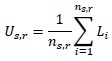
where n_sis the number of GBIF occurrence records for species s, and L_i is the VIIRS nighttime lights radiance value extracted at the location of occurrence i. We also clarify in the Methods that this urban score is an absolute summary statistic of observed urbanization at species occurrence locations

(3) Methods - urban tolerance

How the authors are defining and calculating tolerance is unclear, confusing, and flawed in my opinion.

Tolerance is a common concept in ecology, evolution, and physiology, typically defined as the ability for an organism to maintain some measure of performance (e.g., fitness, growth, physiological homeostasis) in the presence versus absence of some stressor. As one example, in the herbivory literature, tolerance is often measured as the absolute or relative difference in fitness of plants that are damaged versus undamaged

(e.g., https://academic.oup.com/evolut/article/62/9/2429/6853425?login=true).

On line 309, after describing the calculation of urban scores across subrealms, they write: "Therefore, a species could be represented across multiple subrealms with differing measures of urban tolerance (Fig. S4). Importantly, this continuous metric of urban tolerance is a relative measure of a species' preference, or affinity, to urban areas: it should be interpreted only within each subrealm". This is problematic on several fronts. First, the authors never define what they mean by the term "tolerance". Second, they refer to urban tolerance throughout the paper, but don't describe the calculation until, where they write (text in [ ] is from the reviewer): "Within each subrealm, we further accounted for the potential of different levels of urbanization by scaling each species' urban score by subtracting the mean VIIRS of all observations in the subrealm (this value is hereafter referred to as urban tolerance). This 'urban tolerance' (Fig. S5) value can be negative - when species under-occupy urban areas [relative to the average across all species] suggesting they actively avoid them-or positive-when species over-occupy urban areas [relative to the average across all species] suggesting they prefer them (i.e., ranging from urban avoiders to urban exploiters, respectively). They are taking a relativized urban score and then subtracting the mean VIIRS of all observations across species in a subrealm. How exactly one interprets the magnitude isn't clear and they admit this metric is "not interpretative across subrealms".

This is not a true measure of tolerance, at least not in the conventional sense of how tolerance is typically defined. The problem is that a species distribution isn't being compared to some metric of urbanness, but instead it is relative to other species' urban scores, where species may, on average, be highly urban or highly nonurban in their distribution, and this may vary from subrealm to subrealm. A measure of urban tolerance should be independent of how other species are responding, and should be interpretable across subrealms, continents, and the globe.

We thank the reviewer for this careful and important critique. We agree that the term “tolerance” is commonly used to describe the ability of an organism to maintain performance (e.g., fitness, growth, physiological homeostasis) in the presence of a stressor, and that our metric does not measure tolerance in this mechanistic or fitness-based sense. To address this directly and unambiguously, we have revised the manuscript to explicitly define the term “urban affinity” as opposed to urban tolerance. 

In the revised Methods, we also reorganized and clarified the calculation of urban affinity, introduced explicit notation, and provided a formal equation. Specifically, we now define urban affinity for species s in subrealm r as:

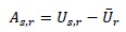
where U_s,ris the mean VIIRS radiance across all occurrence locations of species s within subrealm r, and Ū_ris the mean VIIRS radiance across all occurrence records of all species in that subrealm. This transformation centers species’ urban scores on the regional background level of urbanization, yielding a relative measure of spatial association with urban environments.

We agree with the reviewer that this metric is not interpretable as an absolute measure of affinity, and we now state this explicitly. Urban affinity values are, by construction, relative measures, interpretable only within subrealms, and they quantify whether a species tends to occur in more or less urbanized environments than is typical for that region. The magnitude of the metric therefore reflects deviation from the regional baseline, not a universal or global scale of urbanization, and is not intended to be compared directly across subrealms.

We respectfully disagree, however, that this makes the metric flawed. Rather, it reflects a deliberate analytical choice aligned with our research questions. Our goal was not to estimate absolute urban exposure or physiological performance, but to compare species’ realized spatial associations with urban environments within shared biogeographic contexts. Because baseline urbanization levels, settlement history, and species pools vary strongly across regions, a globally absolute metric would conflate species’ affinities with regional availability of urban environments. By contrast, a relative, region-centered metric allows meaningful comparisons among species that coexist within the same ecological and biogeographic setting. This approach follows a growing body of macroecological work that infers species’ environmental affinities from spatial distributions rather than direct performance measures (e.g., Callaghan et al. 2020; 2021; 2023), and we now cite these studies explicitly.

I propose the authors use one of two metrics of urban tolerance:

(i) Absolute Urban Tolerance = Mean VIIRS of species_i - Mean VIIRS of city centers Here, the mean VIIRS of city centers could be taken from the center of multiple cities throughout a subrealm, across a continent, or across the world. Here, the units are in the original VIIRS units where 0 would correspond to species being centered on the most extreme urban habitats, and the most extreme negative values would correspond to species that occupy the most non-urban habitats (i.e., no artificial light at night). In essence, this measure of tolerance would quantify how far a species' distribution is shifted relative to the most highly urbanized habitat available.

(ii) % Urban Tolerance = (Mean VIIRS of species_i - Mean VIIRS of city centers)/MeanVIIRS of city centers * 100%

This metric provides a % change in species mean VIIRS distribution relative to the most urban habitats. This value could theoretically be negative or positive, but will typically be negative, with -100% being completely non-urban, and 0% being completely urban tolerant.

Both of these metrics can be compared across the world, as it would provide either absolute (equation 1) or relative (equation 2) metrics of urban tolerance that are comparable and easily interpretable in any region.

In summary, the definition of tolerance should be clear, the metric should be a true measure of tolerance that is comparable across regions, and an equation should be given.

We thank the reviewer for this thoughtful and constructive suggestion, which raises an important conceptual issue regarding how “urban tolerance” should be defined and quantified. We agree that any such metric must be clearly defined, interpretable, and accompanied by an explicit equation, and we have revised the manuscript accordingly to clarify both our definition and its intended interpretation.

The alternative metrics proposed by the reviewer anchoring species’ distributions to city centers or to the most highly urbanized habitats represent a valid and intuitive absolute framing of urban tolerance. Indeed, a closely related approach was explored and evaluated in Callaghan et al. (2020; https://doi.org/10.1016/j.ecolind.2020.106905), where species’ occurrence-based urbanness scores derived from VIIRS night-time lights were compared against abundance-based estimates of urban tolerance using explicit urban–non-urban contrasts. That study further demonstrated that urbanness scores depend on the choice of spatial baseline (e.g., regional buffers around cities versus continental extents), and showed that different baselines capture complementary, but not identical, aspects of species–urban associations.

In the present study, we deliberately adopt a relative, regionally contextualized metric (now referred to as urban affinity), expressing each species’ mean VIIRS association relative to the background urbanization of the biogeographic subrealm in which it occurs. This choice reflects our goal of comparing species’ relative affinities to urban environments within shared ecological and biogeographic contexts. Importantly, identical VIIRS values can correspond to very different ecological conditions across regions, and anchoring all species to city centers or global urban maxima risks conflating species’ affinities with regional differences in urban availability and infrastructure.

We now make this distinction explicit throughout the manuscript, including by (i) defining urban affinity as a relative, occurrence-based measure of urban affinity (rather than physiological or fitness-based tolerance), (ii) providing an explicit equation for its calculation, and (iii) clarifying that these values are interpretable within, but not across, biogeographic subrealms. We view absolute, city-center–anchored metrics and relative, regionally normalized metrics as complementary approaches, each suited to different questions; the latter is most appropriate for the macroecological, comparative analyses pursued here.

(4) Figure 1: The figure does not stand alone. For example, what is the hypothesis for thermophily or the temperature-size rule? The authors should expand the legend slightly to make the hypotheses being illustrated clearer.

We now expanded the legend so that the figure and hypotheses presented can be understood based on just the figure and its legend; we did so by explaining the illustrated hypotheses as requested by the Reviewer. The figure legend now reads as follows:

“Fig. 1: Conceptual framework illustrating hypothesized mechanisms linking urban affinity to interspecific body-size shifts. These include dispersal and mobility constraints under habitat fragmentation [44,45], thermophily and the temperature–size rule driven by the urban heat island effect [15,30], size-biased competition and survival [94,95], and size-biased human preferences [64]. Urban fragmentation of habitat resources can select for increased mobility (e.g., larger butterflies) or reduced mobility (e.g., larger seeds) depending on isolation severity. Elevated urban temperatures favor thermophily, which often negatively correlates with size as it affects the heat balance via thermal inertia. Similarly, these higher temperatures generally favor smaller-bodied adult ectotherms because they accelerate development and reduce time available for growth (i.e., temperature-size rule). In plants, the increased CO_₂ and nutrient availability associated with anthropogenic environments due to heating- and traffic-related CO2 emissions and eutrophication provides a competitive advantage to larger plant species, and human preferences too may favor larger species (e.g., tree-lined streets), whereas smaller species may be advantaged in colonizing built infrastructure.”

(5) SUDs: I don't agree with the conclusion given on line 83 ("pattern was consistent across subrealms and several taxonomic levels") or in the legend of Figure 2 ("there were consistent patterns for kingdoms, classes, and orders, as shown by generally similar density histograms shapes for each of these").

The shapes of the curves are quite different, especially for the two Kingdoms and the different classes. I agree they are relatively consistent for the different taxonomic Orders of insects.

We agree that our original wording overstated the similarity of distributions across taxa and regions. We have revised the text to clarify that the consistency we refer to pertains primarily to central tendencies rather than identical distributional shapes. To address this directly, we conducted additional analyses comparing urban affinity distributions across subrealms for taxonomic groups with the largest sample sizes. These results, now presented in new Supplementary Figures (Fig. S2-S4), show that while distributional shapes vary among higher taxonomic groups, median values and overall spread are broadly similar within comparable taxonomic levels. We have updated the Results text and the Figure 2 legend accordingly to reflect this more precise interpretation. 

“These patterns in central tendency were broadly consistent across subrealms and taxonomic levels, although distributional shapes varied among higher taxonomic groups (Fig. 2).”

“To evaluate this more formally, we compared distributions across subrealms for groups with the largest sample sizes and found that while distributional shapes varied among higher taxa, median values and overall spread were broadly similar within comparable taxonomic levels (Fig. S2–S4).”

Figure 2 caption: “There were consistent patterns for kingdoms, classes, and orders (B) as shown by similar central tendencies despite variation in distributional shape.”

We refer the Reviewer to the revised manuscript and supplementary material, but show the kindom level in Fig S2.

More broadly, our goal in introducing Species Urbanness Distributions (SUDs) is not to argue that their exact shapes are invariant, but rather to provide a generalizable framework for describing how assemblages are structured along an urbanization gradient. In this respect, SUDs are conceptually analogous to Species Abundance Distributions (SADs), where the precise functional form has long been debated, yet the framework itself has proven extremely valuable for ecology. We therefore emphasize the utility of SUDs as a descriptive and comparative tool for quantifying community-level responses to urbanization, rather than as a claim about strict uniformity in distributional shape across taxa or regions.

Reviewer #3 (Public review):

Summary:

This paper reports on an association between body size and the occurrence of species in cities, which is quantified using an 'urban score' that can be visualized as a 'Species Urbanness

Distribution' for particular taxa. The authors use species records from the Global Biodiversity Information Facility (GBIF) and link the occurrence data to nighttime lighting quantified using satellite data (Visible Infrared Imaging Radiometer Suite-VIIRS). They link the urban score to body size data to find 'heterogeneous relationship between body size and urban tolerance across the tree'. The results are then discussed with reference to potential mechanisms that could possibly produce the observed effects (cf. Figure 1).

We thank the reviewer for this clear and accurate summary of the study. We agree that the primary contribution of this work lies in the scale and taxonomic breadth of the analysis, and in introducing a framework (Species Urbanness Distributions) for quantifying species’ relative affinities to urban environments using globally available data. We have revised the manuscript to further clarify the scope of inference and the distinction between descriptive macroecological patterns and mechanistic explanations.

Strengths:

The novelty of this study lies in the huge number of species analyzed and the comparison of results among animal taxa, rather than in a thorough analysis of what traits allow species to persist under urban conditions. Such analyses have been done using a much more thorough approach that employs presence-absence data as well as a suite of traits by other studies, for example, in (Hahs et al. 2023, Neate-Clegg et al. 2023). The dataset that the authors produced would also be very valuable if these raw data were published, both the cleaned species records as well as the body sizes. The paper could strongly add to our understanding of what species occur in cities when the open questions are addressed.

We appreciate highlighting the novelty of the taxonomic breadth and scale of our analysis. We agree that our approach is complementary to more detailed, taxon-specific trait studies based on presence–absence data. In response, we have further emphasized this distinction in the Discussion:

“Our synthesis complements taxon-specific, presence–absence trait studies by identifying broad, cross-taxonomic patterns that can motivate and contextualize more mechanistic analyses17,23.”

We also agree that the cleaned occurrence data and body size information represent a valuable resource, and all data will be made available, with the exception of some body size datasets which we are not able to make available.

Weaknesses:

I value the approach of the authors, but I think the paper needs to be revised.

In my view, the authors could more carefully validate their approach. Currently, any weakness or biases in the approach are quickly explained away rather than carefully explored. This concerns particularly the use of presence-only data, but also the calculation of the urban score.

The vast majority of data in GBIF is presence-only data. This produces a strong bias in the analysis presented in the paper. For some taxa, it is likely that occurrences within the city are overrepresented, and for other taxa, the opposite is true (cf. Sweet et al. 2022). I think the authors should try to address this problem.

We thank the reviewer for raising this important point. We fully agree that GBIF occurrence data are subject to well-known sampling biases, including uneven geographic coverage, observer effort, and taxonomic focus. These limitations are now more explicitly acknowledged in the revised manuscript. At the same time, GBIF currently represents the only global biodiversity database that allows the scope of analysis undertaken here, spanning thousands of species across multiple taxonomic groups and regions. Systematic monitoring datasets that provide presence–absence data are typically restricted to particular taxa (often vertebrates or plants) and are geographically concentrated in the Global North, which would substantially limit the taxonomic and geographic breadth of our analysis.

Importantly, our objective was not to estimate absolute species-specific responses to urbanization, but rather to examine relative patterns of urban affinity across species and families within comparable regional contexts. To address this, we structured our analyses at the subrealm level, which aggregates observations across large spatial extents and reduces sensitivity to fine-scale sampling biases associated with individual cities or urban–rural gradients. In addition, we restricted analyses to species with ≥100 observations per subrealm to focus on well-sampled taxa and reduce the influence of extremely sparse occurrence records. While these steps cannot fully eliminate sampling biases inherent to occurrence data, they substantially mitigate their influence when examining broad comparative patterns.

Recent work has also evaluated the performance of GBIF data in urban biodiversity contexts. For example, Sweet et al. (2022) compared GBIF-derived species richness patterns with independent state-level biodiversity databases across cities and surrounding regions, finding that GBIF provided comparable or broader coverage across taxa and spatial extents. Their analysis showed that species richness was consistently higher in the surrounding region than in the city itself, suggesting that GBIF data capture broad urban–regional biodiversity gradients rather than systematically overrepresenting urban occurrences. Although our analysis differs in design, these results support the use of GBIF as a valuable resource for examining large-scale biodiversity patterns.

More broadly, occurrence databases such as GBIF have become widely used for analyzing species–environment relationships at macroecological scales. While they may be insufficient for estimating precise species-specific environmental tolerances, they are informative for identifying broad patterns across taxa and regions. Our goal here is therefore to identify large-scale comparative patterns in urban affinity and generate hypotheses about trait– urbanization relationships, which can subsequently be tested with more structured monitoring datasets where available.

Another important consideration is that our analyses focus on comparative differences among species within shared taxonomic and geographic contexts, rather than absolute estimates of urban affinity. Sampling biases in occurrence databases are often structured by observer behaviour (e.g., detectability, accessibility, or taxonomic interest), meaning that species recorded by similar observer communities are likely subject to similar sampling biases. Under these conditions, relative differences among species are expected to be preserved even when absolute occurrence frequencies are biased. This logic is consistent with the widely used target-group background approach in presence-only species distribution modelling, where species recorded by similar observer groups (often within the same taxonomic group) are used to control for shared sampling bias. Previous work by Callaghan et al. (2021; https://doi.org/10.1111/gcb.15670) performed additional validation analysis comparing our distribution-based urban affinity metric with estimates derived from occupancy modelling using well-sampled European butterflies (see Fig. S5 from the Callaghan et al. 2021 paper). The strong positive relationship between these approaches suggests that the broad patterns identified here are unlikely to arise solely from sampling artifacts.

Finally, in the revised manuscript we now include additional comparisons among well-sampled taxonomic groups (see responses to other comments throughout our response document for details), which show substantial variation in urban affinity even among taxa with extensive sampling. These results suggest that the patterns reported here are unlikely to arise solely from sampling artifacts, but instead reflect meaningful ecological variation in how species interact with urban environments.

The authors should compare their results to studies focusing on particular taxa where extensive trait-based analyses have already been performed, i.e., plants and birds. In fact, I strongly suggest that the authors should compare their results to previous studies on the relationship between traits, including body size and occurrences along a gradient of urbanisation, to draw conclusions about the validity of the approach used in the current study, which has a number of weaknesses.

We agree that explicitly situating our findings within the existing trait-based urban ecology literature strengthens both interpretation and validation of our approach. We had already referenced several relevant studies (e.g., Hahs et al. 2023 and others) in the Introduction and Discussion, but we recognize that these comparisons were not sufficiently explicit. We have now added text to the Discussion directly comparing our results with previous trait-based studies across taxa:

“Our results are broadly consistent with prior taxon-specific trait-based studies (eg., Hahs et al.[17]), but also highlight that relationships between body size and urbanization vary across taxa and analytical frameworks. For example, global syntheses and regional studies have reported positive, negative, or null size–urbanization relationships depending on clade and spatial scale. A recent global analysis that compiled empirical occurrence data for multiple terrestrial faunal taxa across cities worldwide reported broadly similar body-size responses to urbanization [17]. For four of the five groups that overlap with our analysis—amphibians, bats, bees, and birds—the direction of the body-size relationship with urbanization was consistent between studies. The only exception was carabid beetles, which tended to be smaller-bodied in highly urbanized environments in that analysis, whereas we detected no significant size effect for this family. Studies on birds, for example, have found mixed results, including positive associations to urbanization in some regional assemblages [45], no global relationship in others [46] or an overall negative relationship globally [23], and negative relationships in particular clades such as raptors [40]. Such discrepancies likely arise because different studies quantify urbanization differently, focus on different spatial grains, or analyze different components of species responses (e.g., presence– absence, abundance, or occurrence distributions). Additionally, a study on multiple taxa including butterflies and moths found a positive relationship in butterfly and moth community-weighed mean body size with increases in urbanization level, similar to our findings [31]. Researchers have also found that smaller-bodied dung-associated beetles potentially benefit from urban environments, which is similar to the negative association we found between urbanization and body size in beetles [47]. Our approach complements these studies by estimating occurrence-based urban associations across thousands of taxa simultaneously, allowing comparison of how consistently body size predicts urban affinity across taxonomic groupings rather than within a single lineage. In this sense, variation among published results does not contradict our findings but instead reinforces the conclusion that body size is a context-dependent filter whose direction and strength depend on ecological setting, taxonomic scope, and the urbanization metric used.”

These additions highlight that published relationships between body size and urbanization vary widely across taxa, spatial scales, and analytical approaches. For example, prior studies have reported positive, negative, or null size–urbanization relationships depending on clade, geographic extent, and how urbanization or occurrence is quantified. Even within birds alone, the literature spans positive regional relationships, null global relationships, and negative relationships in particular clades such as raptors. We now explicitly discuss these contrasts and clarify that such discrepancies are expected because different studies measure different components of species’ responses (e.g., presence–absence vs. abundance vs. occurrence distributions), use different spatial grains, or focus on different taxonomic subsets.

We emphasize that our analysis is not intended to replace taxon-specific trait studies, but rather to complement them by providing a macroecological synthesis across thousands of species simultaneously. Importantly, the heterogeneity we observe among families is itself a key biological result, indicating that body size is not a universal predictor of urban affinity but instead a context-dependent filter whose direction and strength vary across ecological and phylogenetic settings. We now state this interpretation more clearly in the revised manuscript.

They should be be more careful in coming up with post-hoc explanations of why the pattern found in this study makes sense or suggests a particular mechanism. This reviewer considers that there is no way in which the current study can disentangle the different possible mechanisms without further analyses and data, so I would suggest pointing out carefully how the mechanisms could be studied.

We agree that our study cannot disentangle the causal mechanisms underlying species’ responses to urbanization. Our intent in discussing potential mechanisms was not to claim definitive explanations, but rather to situate our findings within existing ecological theory and to highlight plausible, non-exclusive pathways that may generate the observed patterns. To make this clearer, we have revised the Discussion to explicitly frame these interpretations as hypotheses rather than conclusions, and to emphasize that testing the underlying mechanisms will require additional data and approaches, such as targeted trait datasets, experimental manipulations, and longitudinal or within-city studies:

“Because our synthesis is correlative and macroecological in nature, the mechanisms discussed above are best viewed as hypotheses that can be evaluated through future work combining experimental, trait-based, and longitudinal data.”.

Additionally, we modified our overall goal to make it clear that this is not inherently a mechanistic study per se:

“Our aim is to identify broad, cross-taxonomic patterns in species’ urban affinity at a global scale, rather than to resolve the specific causal mechanisms driving urban success or failure within individual taxa or cities.”.

More details should be given about the methodology. The readers should be able to understand the methods without having to read a number of other papers.

We have substantially revised and expanded the Methods section to ensure that all analytical steps can be understood directly from the manuscript without requiring consultation of prior publications. In particular, we now (i) provide a clear conceptual roadmap of the workflow at the start of the Methods, (ii) define all key metrics explicitly, including equations for both the urban score and urban affinity, and (iii) clarify the interpretation, assumptions, and limitations of each step. We also added text explaining the rationale for subrealm stratification and the intended interpretation of relative values. Together, these revisions make the methodological framework fully transparent and self-contained (see revised Methods and related responses above and below).

References:

Hahs, A. K., B. Fournier, M. F. Aronson, C. H. Nilon, A. Herrera-Montes, A. B. Salisbury, C. G. Threlfall, C. C. Rega-Brodsky, C. A. Lepczyk, and F. A. La Sorte. 2023. Urbanisation generates multiple trait syndromes for terrestrial animal taxa worldwide. Nature Communications 14:4751.

Neate-Clegg, M. H. C., B. A. Tonelli, C. Youngflesh, J. X. Wu, G. A. Montgomery, Ç. H. Şekercioğlu, and M. W. Tingley. 2023. Traits shaping urban tolerance in birds differ around the world. Current Biology 33:1677-1688.

Sweet, F. S. T., B. Apfelbeck, M. Hanusch, C. Garland Monteagudo, and W. W. Weisser. 2022. Data from public and governmental databases show that a large proportion of the regional animal species pool occur in cities in Germany. Journal of Urban Ecology 8:juac002.

We have incorporated these (and additional new references) into our revised manuscript.

Recommendations for the authors:

Reviewing Editor Comments:

As you see from the general comments above and the specific recommendations below, the reviewers are impressed by your comprehensive data set and the analytic approach. However, they ask you to clarify your measures of organism size, occurrence data (vs. presence/absence and corresponding sample-bias caveats), urbanness (lighting differences between cities and regions?), urban tolerance (measure should not be relative to other species and particular regions), and region ("subrealm" vs. more commonly used defintions of world regions such as continents). They also encourage you to compare your general results with more detailed local studies to better justify using size as the only, easily available trait.

We thank the Editor for this clear synthesis of the key priorities for revision. We have carefully addressed each point and substantially revised the manuscript to improve clarity, methodological transparency, and interpretability. In particular:

We clarified how body size data were compiled, harmonized, and modeled, including explicit description of how different measurement types (mean, maximum, sex-specific) were retained and statistically accounted for through scaling and hierarchical modeling. We now state these procedures explicitly in the Methods.

We expanded the Methods and Discussion to clarify that our analyses rely on occurrence data rather than presence–absence or abundance data, and we now explicitly discuss the implications and limitations of presence-only datasets, including potential sampling biases and how these may influence inference.

We strengthened justification for using VIIRS night-time lights as a continuous proxy for urbanization, added supporting citations, and clarified that spatial heterogeneity in lighting primarily introduces additional variance rather than systematic bias. We also explicitly describe how urbanization values were calculated and interpreted.

We substantially revised the manuscript to clearly define urban affinity at the outset (including in the Abstract), distinguish it from physiological definitions of tolerance, and provide explicit equations and step-by-step descriptions of how both urban score and urban affinity are calculated and interpreted. We now emphasize that the metric is a relative, region-contextualized measure of occurrence-based urban affinity.

We added full justification, citations, and methodological explanation for the use of biogeographic subrealms, clarified how they differ from continents or climate zones, and explained why this stratification is appropriate for the ecological questions addressed. We also clarified the scope of inference and limitations of this approach.

We expanded the Discussion to explicitly compare our results with prior trait-based urban ecology studies across taxa (including birds and other groups), highlighting where results converge, diverge, and why such variation is expected across spatial scales, taxa, and analytical frameworks.

Reviewer #1 (Recommendations for authors):

(1) Abstract

(a) Please define how tolerance is being used here

We now use affinity throughout and it is defined in various places (see responses to other comments here).

(b) The abstract should clarify at what taxonomic scale body size is assessed. It is unclear in the abstract as to whether the reader expects intraspecific measures and interspecific, and at what resolution.

We have revised the abstract by adding one sentence explicitly stating the scale body size was assessed:

“We then assessed whether body size, an integrative ecological trait fundamental to space use, mobility, metabolism, and environmental sensitivity, showed consistent associations with urban affinity among species and across 371 taxonomic families. Analyses were conducted at the interspecific level and focused primarily on variation among taxonomic families (provided with this paper is an accompanying application to view results).”

(2) Results/Discussion

(a) The species urbanness distribution and comparison with the species abundance distribution is an interesting and conceptually useful contribution to urban ecology and underscores how urbanization functions on biodiversity at scale.

We thank the reviewer for this positive assessment and are encouraged that they view the Species Urbanness Distribution (SUD) as a conceptually useful contribution to urban ecology. We see SUDs as a flexible framework that can be extended in several important directions, including comparisons across additional traits, cities of differing size and configuration, and temporal analyses that track how urbanness distributions shift with ongoing urban expansion or restoration. More broadly, we hope that SUDs can provide a framework to think about a macroecological understanding of how urbanization filters biodiversity.

(b) In our Lambert et al. (2023) study that you reference, we suggest that 'exaptation' may be valuable to explore in urban areas. Although body size wasn't the trait we were considering at that time, it may be worth putting your discussion around pre-adaptation in this context.

We agree that exaptation provides a valuable conceptual lens for interpreting species’ responses to urban environments. We have revised the Discussion to explicitly frame species’ urban success in this context:

“Such traits “pre-adapted” to urban conditions allow for some species to not only persist but thrive in urban environments where most species cannot. Framing these patterns through the lens of exaptation may be particularly useful, as traits that evolved under non-urban selective pressures may incidentally confer advantages in urban environments without having arisen in response to urbanization per se (sensu Lambert et al.[4]). We therefore speculate that the skewed shape of SUDs may reflect the uneven distribution of exaptive traits across species pools, rather than widespread adaptive evolution to urban conditions. 

Consistent with this interpretation, if exaptive traits that facilitate urban persistence are unevenly distributed across species pools, most species would be expected to exhibit avoidance rather than affinity of urban environments. Indeed, we found that the median urban affinity is most often below one, indicating widespread avoidance among species.”.

(c) Given the family-scale effect, it would be helpful to discuss how often species within a family co-occur in a given geographic region, how much other traits covary with size, etc. Do we have an a priori reason to expect family to be the taxonomic resolution at which body size seems to be most varied?

Our exploratory and preliminary analyses revealed that variation in the body size– urban affinity relationship was strongest at the family level, which prompted us to focus our main analyses at this taxonomic resolution. (But we also present results on order as well). Families represent a biologically meaningful intermediate scale in taxonomy: species within families typically share broad morphological, ecological, and life-history characteristics, yet still exhibit substantial variation in body size and ecological strategies. Indeed, body size is well known to covary with multiple traits—including dispersal ability, metabolism, and space use—making it an integrative trait that captures several ecological dimensions simultaneously within and among families. These correlated traits likely contribute to the heterogeneous responses to urbanization observed among families.

Using the family level also provides a practical balance between biological relevance and statistical robustness. Many families contain sufficient numbers of species to allow independent model estimation while avoiding the strong data imbalance that would arise at higher taxonomic levels. In addition, family is a commonly used unit in macroecological trait analyses (e.g., Roy et al. 2009; Smith et al. 2004), and it often reflects major morphological and ecological similarities among species, as reflected in taxonomic identification frameworks.

Regarding co-occurrence, our analytical framework already accounts for geographic context by estimating urban affinity within subrealms. This ensures that species are compared within the same regional species pools and environmental contexts, rather than across globally disparate assemblages. Consequently, family-level effects emerge from comparisons among species that co-occur within shared biogeographic settings rather than from global taxonomic aggregation.

We have added a short clarification in the manuscript to emphasize that body size functions as an integrative trait that covaries with multiple ecological attributes, and that family-level analyses represent a balance between ecological interpretability and data availability:

“Because body size covaries with multiple ecological traits (e.g., dispersal ability and metabolic rate), we focused on family-level analyses to capture shared ecological strategies while still allowing sufficient variation among species to detect trait– environment relationships [39]”.

(d) The result that body size shows a stronger effect in plants perhaps could suggest that plant records in GBIF are more sensitive to potential collection bias, perhaps due to detectability differences or preferences for where botanists and citizen scientists collect plant data? You mention ornamental plants late, but it may be worth discussing this here, too.

We agree that this is a possible mechanism, which likely conflates detectability and ecological signal. We have expanded this point in the discusssion to better address this:

“These human-driven preferences may also influence detectability and recording effort, as larger and more conspicuous plant species are more likely to be planted, maintained, and documented in urban environments, and thus be available in GBIF for our analyses. However, we suggest that this is not purely a sampling artifact, but such processes likely interact with ecological filtering to shape the realized size structure of urban plant communities.”.

(e) I appreciate the additional taxonomic layering to the discussion. Seeing patterns at the family and order levels is helpful for generating new theory and predictions about how urbanization structures biodiversity at different taxonomic scales.

We agree that examining patterns across multiple taxonomic scales is particularly valuable for generating testable hypotheses about how urbanization structures biodiversity, as different mechanisms may emerge or break down depending on the resolution of analysis. We hope this multi-scale perspective helps stimulate new theory and predictions about the ecological processes shaping urban biodiversity across the tree of life.

(3) Methods

(a) The methodology provides a scalable, consistent, and reasonable measure of both urbanness and species-level urban tolerance. The urban tolerance measure will, of course, not be useful for certain types of research (e.g., animal behavior), but it is appropriate for the resolution of this study.

We agree that the urban affinity metric presented here is intended for broad-scale, comparative analyses and is not designed to capture fine-scale processes such as individual behavior or short-term demographic responses. Our goal was to develop a scalable and consistent measure that enables cross-taxon and cross-region comparisons at a global extent, which we believe is appropriate for addressing the questions posed in this study. We have sought to be explicit about this scope throughout the manuscript (e.g., to better alleviate Reviewer #1 concerns) and emphasize that the framework is complementary to, rather than a replacement for, more mechanistic or organism-focused approaches.

(b) I'm concerned that the authors were not able to constrain their dataset to mean, median, or maximum, not potentially sex variability in sizes. Later in the methods, the authors state that they selected the measure of size that was most common within a family. Does this mean that species within a given family that didn't have that measure of body size were removed from the analysis?

We appreciate this important point and agree that heterogeneity in how body size is measured (e.g., mean, maximum, or sex-specific estimates) is a real and unavoidable challenge in large-scale trait syntheses. Our analytical approach was explicitly designed to minimize the influence of this heterogeneity while retaining as many species as possible, rather than excluding species based on inconsistent trait metadata.

Specifically, species within a family were not removed based on the availability of a particular body size definition. All species with at least one body size estimate were retained. When multiple measures existed for a species, we selected the measurement type that was most commonly available within each family to maximize comparability while preserving sample size. Remaining heterogeneity among measurement types (including units, measurement detail, and whether values reflected means, maxima, or sex-specific estimates) was explicitly accounted for through log-transformation and metadata-aware centering and scaling, with measurement metadata included as random intercepts in the hierarchical models. We have clarified this point in the Methods:

“Importantly, this procedure did not result in the exclusion of species lacking a particular body size definition; rather, all species with at least one available body size estimate were retained, with measurement heterogeneity explicitly accounted for through metadata-aware scaling and hierarchical modeling.”

In addition, our taxonomic modeling strategy was intentionally hierarchical. Species belonging to families that did not meet the minimum threshold for family-level modeling (≥10 species) were not discarded; rather, they were included in higher-level taxonomic analyses (e.g., order- or class-level models), ensuring that available information was retained wherever statistically appropriate. This approach reflects our broader goal of maximizing data inclusion while matching inference to the resolution supported by the data.

Reviewer #2 (Recommendations for the authors):

(1) Overlap between VIIRS and GBIF data: While it would have been nice for the GBIF records and VIIRS timescales to match, the degree of mismatch isn't overly large (2010-2021 vs 2015-2021), and any bias or inaccuracies should be minimal. I am mainly making this comment as a potential counterpoint to a possible criticism from other reviewers.

We thank the reviewer for this helpful observation and agree with their assessment. While the temporal coverage of GBIF occurrence records (2010–2021) and VIIRS night-time lights data (2015–2021) does not perfectly overlap, the mismatch is relatively small and unlikely to introduce substantial bias, particularly given our focus on broad, global patterns of urban affinity rather than fine-scale temporal dynamics. We appreciate the reviewer highlighting this point as a potential counterargument to concerns about temporal alignment.

(2) Line 87: "only a select few species seem to possess traits that enable them to thrive in urban...".

This seems like an odd statement, given how many of these species have positive urban tolerance measures.

Agreed that this was oddly worded. We have revised for clarity, focusing on the magnitude of urban affinity:

“Similarly, much like the skewed distributions observed in SADs [24,26], the skewed shape of SUDs indicates that while many species exhibit some degree of urban affinity, a relatively small subset of species attain high levels of urban affinity and dominate urban environments.”

(3) Line 81: "skewed shape of SUDs suggests that traits enabling species to tolerate urban environments are both rare and specific".

Again, based on the shape of some of these curves, I'm not convinced that it is rare, and there is nothing about these curves that suggests it is something "specific". Indeed, urban tolerance could be very multivariate, and the authors' own results suggest this is indeed the case.

We have revised the sentence to retain a focus on traits while avoiding overinterpretation of adaptation from the distributional patterns alone. The revised wording emphasizes the uneven expression of high urban affinity across species without implying rarity or trait specificity:

“The skewed shape of SUDs suggests that traits enabling species to tolerate urban environments are unevenly expressed, given that only a handful of species show extreme urban affinity values, but our results suggest this is geographically widespread across taxa.”.

We also agree with the likelihood that it is multivariate, and return to this in the conclusion in a stronger sense:

“Although body size emerged as a predictor of urban affinity, we found not only substantial heterogeneity across families and orders, but also that body size filtering alone is unlikely to explain the consistently skewed SUD shape. Taken together, these patterns suggest that urban affinity likely emerges from multiple trait combinations rather than a single, universally advantageous trait, and that strong affinity to urban environments is not uniformly expressed across taxa, despite occurring broadly across regions.”.

(4) Line 100: "UHI", avoid abbreviations unless absolutely necessary.

We have removed this abbreviation throughout.

(5) Body size: focusing on one trait seems like a shot in the dark, and so it isn't too surprising that this didn't reveal a strong or consistent pattern. However, I also recognize that collecting consistent trait data across so many taxa is challenging, and size is a low-hanging fruit that correlates with multiple traits. Perhaps discuss more the range of traits you think are most likely to predict urban tolerance.

Body size is indeed the ‘easiest’ to collect, but we acknowledge that there are other traits which could be important, and body size correlates with multiple traits. We revised our discussion to be more comprehensive to discuss some of the additional traits, and be explicit about the shortfalls of body size:

“Ultimately, the heterogeneous and sometimes weak relationships between body size and urban affinity suggests that body size alone cannot explain the emergence of extreme urban exploiters and the skewed shape of SUDs. Focusing on body size as a focal trait necessarily represents a simplification of the multidimensional processes underlying species’ responses to urbanization, driven in part by data availability when conducting a taxonomically-broad synthesis. Instead, urban affinity likely depends on multivariate trait combinations [17,58] that vary among taxa [59] and ecological contexts [60]. Traits that are likely to correlate with urban affinity include dispersal capacity, behavioral flexibility, diet breadth, reproductive strategy, thermoregulatory ability, and, in plants, life history traits such as growth form, clonality, phenology, and seed size. The diversity of trait pathways through which species may persist or thrive in urban environments is consistent with the pronounced taxonomic heterogeneity we observe and helps explain why body size alone does not yield a universal pattern.”

(6) Figure S2: This figure and analysis appear to 'come out of nowhere'. I think this is distracting and tangential, and it should be removed. I have the same thoughts about Figure S3. While I do think a discussion of other traits to measure is well warranted and needed, the inclusion of "preliminary' results that aren't motivated by clear questions, appropriate context, and rigorous analysis should be discouraged.

We have removed Figure S2 and Figure S3 in response to this comment.

I hope the authors find my constructive comments useful in their revision process.

This was a very thorough and thoughtful review. We are greatly appreciative of the opportunity and guidance to improve our work!

Reviewer #3 (Recommendations for the authors):

Here is a list of a number of further points that the authors may want to address:

(1) Figure 1 somehow misses the fact that humans simply do not want very large animals in the city. We kill large predators if they come too close to cities, and the same for large herbivores such as wild boar or deer.

We agree that direct human persecution and management of large-bodied species can influence which species occur in urban environments, particularly for large predators and herbivores. Such processes represent important mechanisms shaping urban species assemblages and represent an entire field of socio-ecological dynamics. We have now clarified this point in the Discussion by noting that human–wildlife conflict, management, and persecution could contribute to observed size–urbanization relationships for some taxa, and that disentangling these mechanisms represents an important direction for future research. We added some text to highlight this point):

“Similarly, human–wildlife conflict and active management of large-bodied animals in cities may influence which species persist in urban environments, potentially constraining the upper end of the body size distribution. Taken together, these examples illustrate the importance of considering the socio-ecological context of urban species assemblages [65]”.

(2) Line 270. So you removed all data from the grid-based survey?

We did not remove all data originating from grid-based surveys or gridded products. Rather, we retained GBIF point-occurrence records and applied a standard spatial filtering step, removing only those individual observations with reported coordinate uncertainty greater than 1 km. This was done to ensure reliable alignment between species occurrence points and remotely sensed environmental layers. We have clarified this distinction in the Methods to avoid confusion:

“Due to uncertainty in matching observations with remotely-sensed products, any GBIF observation with a coordinate uncertainty > 1 km was removed. This filtering step removed individual observations with high spatial uncertainty, rather than excluding entire datasets or survey types.”.

(3) Line 278. Human population density?

Yes, we have added ‘human’ here (and elsewhere in this section) to make this clearer to the reader.

(4) Line 284. What is a pixel?

We have modified the text to make this clearer:

“VIIRS Stray Light Corrected Nighttime Day/Night Band Composites product, representing monthly composites, (i.e., this dataset in Google Earth Engine: NOAA/VIIRS/DNB/MONTHLY_V1/VCMSLCFG) with a native resolution of ~500 m². We took the median of all monthly composites for each pixel (i.e., a single grid cell of the night-time lights raster representing a fixed ground area) to calculate a pixel-level urbanization value, measured in average radiance, and used imagery from January 2015 to January 2021 to calculate this median”.

(5) Line 292. It seems to me that lighting is different in different types of cities with the same level of impervious surface, depending on local customs of how many lights are installed, left switched on, etc. I guess that petrol stations and strongly lit industrial areas both produce high levels of light, while for the industrial areas, there could be lawn or other vegetation?

We thank the reviewer for this thoughtful observation and agree that night-time lighting can vary across cities with similar levels of impervious surface due to differences in land use, infrastructure, and cultural lighting practices. We do not interpret VIIRS night-time lights as a direct measure of any single urban feature, but rather as a continuous, integrative proxy for urbanization that captures the combined footprint of human activity, infrastructure intensity, and energy use. VIIRS radiance has been repeatedly shown to correlate strongly with human population density, built infrastructure, and urban extent, while being negatively correlated with vegetation cover (e.g., EVI). It is repeatedly used in remote sensing and urban sustainability literature. This approach is widely supported in the literature, for example:

Panić et al. used night-time lights were to map spatial and temporal patterns of artificial lighting as a proxy for human population distribution and activity, distinguishing areas of urban and rural occupancy.

(https://www.ceeol.com/search/article-detail?id=1035395)

Zhou et al. used night-time light observations were to develop a globally consistent time series of annual urban extent, delineating urban clusters and quantifying global urban growth over decades. (https://doi.org/10.1016/j.rse.2018.10.015)

Chakraborty & Stokes used night-time light time series with machine learning to detect and quantify urban change processes—identifying deviations from expected radiance trends to monitor diverse urban transitions.

(https://doi.org/10.1016/j.rse.2023.113818)

Zhao et al. reviewed night-time light remote sensing was for its broad capacity to quantify human activities and socioeconomic dynamics—such as urbanization, economic change, and environmental impacts—across scales.

(https://doi.org/10.3390/rs11171971)

Zheng et al. used VIIRS nightime lights across 30 global megacities to produce a classification scheme to disentangle urban land changes into five categories, and assess global urbanization processes. (https://doi.org/10.1016/j.isprsjprs.2021.01.002)

Zhao et al. argue that nighttime lights provide a consistent dataset to model and interpret urbanization dynamics and use this to track urban dynamics in Southeast Asia. (https://doi.org/10.1016/j.rse.2020.111980)

While localized mismatches may occur (e.g., brightly lit industrial areas with surrounding vegetation), such heterogeneity is expected to introduce additional variance rather than systematic bias in the measure of urbanization, making our inference conservative. We have clarified this interpretation and added additional supporting references in the Methods:

“Previous work has shown that VIIRS night-time lights is negatively correlated with greenness measured through the Enhanced Vegetation Index (EVI) and positively correlated with human population density [69,71]. Although night-time light intensity can vary among cities with similar impervious surface due to differences in land use, infrastructure, and cultural lighting practices, at broad spatial scales it functions as an integrative proxy of urbanization [75,76,77,78,79,80], with localized heterogeneity contributing primarily to additional variance rather than systematic bias.”

(6) Line 295. How did you reconcile the spatial uncertainty of >1km with an urbanization pixel of 150m2? For how many species did you have a higher uncertainty than pixel size? In my experience, your ca. 39m accuracy is a strong assumption for GBIF data.

We would like to clarify that we do not assume species occurrence accuracy at the scale of the geohash blocks (i.e., tens of meters), and we do not interpret GBIF records as having ca. 39 m positional accuracy. The use of geohash7 (~150 m blocks) reflects a computational indexing choice, not an assumption about biological or observational precision. All GBIF observations with reported coordinate uncertainty greater than 1 km were removed prior to analysis, ensuring that retained occurrences were compatible with the effective spatial resolution of the remotely sensed urbanization data. Importantly, the effective spatial resolution of our urbanization metric remains that of the VIIRS night-time lights product (~500 m). Geohash encoding at a finer resolution was used solely to efficiently associate point occurrences with the appropriate VIIRS pixel while avoiding redundant extraction or averaging across adjacent pixels. This approach does not increase the effective spatial precision of the analysis, nor does it imply sub-pixel inference. We have clarified this in the Methods:

“The VIIRS night-time lights data, with a native resolution of ~500 m², was then matched to these blocks by assigning each geohash7 block the average VIIRS radiance value that intersects it. We do not assume positional accuracy at the scale of the geohash blocks, but geohash encoding was used solely for computational indexing, while the effective spatial resolution of the urbanization metric is that of the VIIRS data (~500 m). This approach allows us to avoid unnecessary redundancy in the data while maintaining the original VIIRS resolution”.

(7) Line 296. Why this high resolution in the species data when your light data is 500m2?

The apparent mismatch in resolution reflects a distinction between data handling resolution and analytical resolution. Species occurrence records were retained at their native point-level precision to avoid premature spatial aggregation and to ensure that each observation could be accurately matched to the appropriate VIIRS night-time lights pixel. The finer-resolution geohash encoding does not imply that species data were analyzed at that scale, nor does it increase the effective spatial resolution of the analysis. We note, however, that the reported spatial uncertainty of some GBIF records may approach or exceed the resolution of the VIIRS data. Retaining such records represents a deliberate trade-off between spatial precision and data coverage, and is necessary to maximize taxonomic and geographic representation in a global analysis of this scope. Importantly, any residual spatial uncertainty is expected to introduce additional noise rather than systematic bias, making our estimates of species–urban affinity relationships conservative.

(8) If you could show how your results match the results of Hahs et al and others with respect to occurrence and traits, this would strengthen your approach.

We agree that explicitly comparing our findings with prior trait-based studies strengthens the interpretability of our approach. We have now added text to the Discussion that directly compares our results with published analyses, including Hahs et al. (2023) and other taxon-specific studies. In particular, we highlight where our occurrencebased estimates recover similar body size–urbanization relationships (four of five taxa in Hahs et al.) and where they differ (e.g., carabids), and we discuss how such differences likely arise from variation in spatial grain, response variables, and definitions of urbanization. These additions clarify how our framework aligns with, complements, and extends existing trait-based work rather than replacing it.

(9) I wonder whether you could run your analysis with simplified data. In the end, you do not talk much about how high the urban score is, so you may also aggregate values to "highly lighted", "lighted", "some light" and "dark" and re-do the analysis, after checking how these scores correlate with e.g. impervious surface in a slightly larger area than what you used (maybe 50x50m).

Our analytical framework—and the concept of Species Urbanness Distributions (SUDs) in particular—relies on retaining the continuous nature of the underlying urbanization metric. Discretizing night-time light values would necessarily introduce arbitrary thresholds, reduce information content, and obscure subtle but ecologically meaningful variation in species’ relative affinities to urban environments. Because we focus on relative affinity patterns rather than absolute urbanization classes, maintaining a continuous metric is central to both our methodological approach and conceptual contribution. That said, we agree that exploring how continuous urban affinity scores relate to categorical urban classes or alternative urbanization proxies (e.g., impervious surface at different spatial grains) represents a valuable direction for future work. Such analyses could be particularly informative for translating continuous affinity metrics into applied conservation or urban planning contexts.

eLife Assessment

This important study investigates how the brain categorizes written words from different writing systems (e.g., alphabetic vs. non-alphabetic). The evidence supporting the authors' claims is solid and sheds light on the neural basis of language's social‑categorization function.

Reviewer #1 (Public review):

Summary:

This study demonstrates, through a series of EEG and MEG experiments, that the human brain automatically categorizes words from alphabetic and non-alphabetic languages, and it unpacks the neural mechanisms of this process from multiple angles. The work examines not only univariate repetition-suppression (RS) effects, but also how repeating or alternating languages influences the representational similarity of words within and across language categories.

Strengths:

The univariate RS effects across multiple experiments lend support to some of the main conclusions.

Comments on revised version.

The authors have made appropriate revisions and supplements in response to the issues I raised, which has largely resolved my concerns.

Reviewer #2 (Public review):

Summary:

This study investigates how the human brain categorizes visual words from distinct writing systems (alphabetic vs. non-alphabetic). Using a repetition suppression paradigm combined with electroencephalography and magnetoencephalography, the authors conducted nine experiments with independent participants to identify the neural network underlying language-based categorization, characterize its temporal dynamics, and test whether this process operates independently of linguistic properties such as semantic meaning and pronunciation.

Strengths:

The study employs a well-validated design with clear control conditions and systematically manipulates key variables including writing system, language familiarity, and native language background. The use of nine experiments with independent participant samples strengthens the reliability and replicability of the results. The work combines EEG and MEG, cross-validating findings across imaging modalities to support the reported neural effects. A combination of univariate, multivariate, and connectivity analyses is used to characterize neural responses and network interactions. Results are consistent across multiple language groups and for both familiar and unfamiliar languages, supporting the generalizability of the identified neural mechanism beyond specific languages or prior experience.

Comments on revised version.

Earlier versions of the manuscript framed these findings as more directly reflecting the social-categorization function of language. In the revised manuscript, the authors now more carefully distinguish language-based word categorization from broader claims regarding social categorization and explicitly acknowledge that the current experiments do not directly test social evaluation or intergroup processes. These revisions improve the conceptual precision of the work and address my major concern from the previous review.

The additional methodological clarifications and supplementary analyses also strengthen the manuscript. Overall, I believe the revised version provides solid evidence for rapid language-based categorization of visual words across different writing systems.

Author response:

The following is the authors’ response to the original reviews.

eLife Assessment

This important study investigates how the brain categorizes written words from different writing systems (e.g., alphabetic vs. non-alphabetic), shedding potential light on the neural basis of language's social‑categorization function. Overall, the evidence supporting the authors' claims is solid, though some analyses and key interpretations would benefit from fuller justification.

Thank you for handling our manuscript! We’ve modified the manuscript according to the reviewers’ comments and suggestions.

Public Reviews:

Reviewer #1 (Public review):

Summary:

This study demonstrates, through a series of EEG and MEG experiments, that the human brain automatically categorizes words from alphabetic and non-alphabetic languages, and it unpacks the neural mechanisms of this process from multiple angles. The work examines not only univariate repetition-suppression (RS) effects, but also how repeating or alternating languages influences the representational similarity of words within and across language categories.

Strengths:

The univariate RS effects across multiple experiments lend support to some of the main conclusions

Weaknesses:

I have reservations about the logic underlying the multivariate analyses, and I believe the implications of the control experiments merit fuller discussion.

(1) Question 1: Logic of the multivariate analyses

The original text states:

"The processing of intra-language similarity was quantified as correlation distances between neural responses to two words of the same language, which occurred more frequently and would be inhibited in the Rep-Cond (vs. Alt-Cond) due to habituation (Fig. 1c)...".

I argue that this passage conflates two levels. Building a representational dissimilarity matrix (RDM) is a data-analysis step; it cannot be equated with a cognitive computation. Hence, there is no sense in which this computation occurs "more frequently" in one condition. RDM construction rests on the pairwise similarity of activity patterns, so even if a task engaged no cognitive computation of representational similarity, we could still compute an RDM. Conversely, if a task factor alters the RDM, we must explain how that factor changes the underlying neural patterns, not claim that it triggers specific cognitive processing. Therefore, I neither understand what "more frequent processing" the authors refer to, nor accept their account of the multivariate results.

The multivariate result pattern, briefly, is that distances between words, both within and across languages, are larger under the repetition condition. One plausible interpretation is that a word representation comprises two parts: language-type (alphabetic vs. non-alphabetic) and fine-grained identity features (visual shape, orthography, semantics, phonology, etc.). Repetition of language type may, via RS, reduce the weight of the first component, thereby increasing the relative contribution of fine-grained features and amplifying inter-word differences. This could explain the multivariate findings.

Thank you for these insightful comments regarding the logic of the multivariate analyses. In the revision, we’ve elaborated the rationale underlying our experimental design. Specifically, we’ve explained why the processing of intra-language similarity is expected to occur more frequently in the repetition condition (Rep-Cond) than in the alternation condition (Alt-Cond) whereas the reverse is true for the processing of inter-language difference. Importantly, we’ve clarified that the processing of intra-language similarity was assessed rather than defined by conducting the multivariate analyses. The multivariate analyses were conducted to assess correlation distances between neural responses to pairs of words, either within the same language or across different languages. We explained what smaller intra-language correlation distances and larger inter-language correlation distances mean for language-base categorization of words (see Page 7-8).

We appreciate the alternative account of the observed neural repetition suppression (RS) effects in terms of language-type versus fine-grained identity (visual shape, orthography, semantics, phonology, etc.) feature processing. We included a paragraph in the revised Discussion to discuss how possible the early neural RS effect can be attributed to the processing of the fine-grained identity features of visual words. This discussion allowed us to clarify that the early neural RS effects related to visual words of familiar and unfamiliar languages highlight the early spontaneous language-based categorization as a unique process of visual words of alphabetic and non-alphabetic languages. However, our results do not exclude the possibility that the processing of the linguistic properties of visual words may contribute to the long-latency RS effect (see Page 37-38).

Page 7-8

“The processing of intra-language similarity occurs when two words of the same language are perceived repeatedly with short interstimulus intervals. Because words of the same language were repeatedly presented in the Rep-Cond and words of two different languages were displayed in the Alt-Cond, the processing of intra-language similarity occurred more frequently and would be inhibited in the Rep-Cond (vs. Alt-Cond) due to habituation (Fig. 1c). By contrast, the processing of inter-language difference takes place when two words of different languages are perceived with short interstimulus intervals. Since words of different languages appeared more frequently in the Alt-Cond (vs. Rep-Cond), we would expect RS of the processing of inter-language difference in the Alt-Cond (vs. Rep-Cond). The neural processing of intra-language similarity was quantified as correlation distances between neural responses to two words of the same language whereas the neural processing of inter-language difference was assessed as correlation distances between neural responses to two words of two different languages. The correlation distances from the multivariate analyses were further employed to assess how words of one language are clustered and how far words of two languages are separated in a two-dimensional (2D) space during language-based word categorization. Enhanced language-based word categorization is associated with smaller intra-language correlation distances, which reflect more densely clustered words of the same language, and larger inter-language correlation distances, which manifest further separated words of two different languages.”

Page 37-38

“How possible are the early neural RS effects within 200 ms after word onset observed in our study related to the processing of low-level perceptual features or high-level linguistic (e.g., orthography, semantics, phonology) properties of visual words? Our analyses of the ERPs to scrambled Chinese and English words in Experiment 2 did not show significant RS effect. Because only low-level visual features were preserved in the scrambled words, the ERP results provided no evidence that the early RS effects on the neural response to words can be attributed to habituation of perception of the low-level perceptual features. Furthermore, we found that the RS effects on the neural response to radicals and letters in Experiment 3 took place in a delayed time window and exhibited different scalp distributions (i.e., over the central region for radicals and occipital regions for letters) compared with the neural RS effects related to words. Thus the early RS effects on the neural response to words cannot be interpreted as habituation of perception of the middle-level units of Chinese and English words (i.e., radicals and letters) either. In addition, the early neural RS effects were similarly observed for both familiar (i.e., Chinese and English) and unfamiliar (i.e., Korean and Italian) languages and occurred earlier than the time window in which the processing of the linguistic properties of visual words takes place (Marinkovic et al., 2003; Hodgson et al., 2021; Zhu et al., 2022). Therefore, the early neural RS effects identified in our work were unlikely to be associated with the processing of the linguistic (e.g., orthography, semantics, phonology) properties of visual words since these properties of unfamiliar languages were unknown to the participants. Taken together, our findings of the early neural RS effects highlight an early word-level representation of alphabetic vs. non-alphabetic languages which distinguishes words from letters/radicals but is similar for familiar or unfamiliar languages. Our results, however, do not exclude the possibility that the processing of the linguistic properties of visual words may contribute to the long-latency RS effect around 300 ms after word onset. Further processing of the linguistic properties of visual words of familiar languages may follow the early language-based categorization of visual words, though this should be tested in future research.”

(2) Question 2:

For unlearned languages, people cannot distinguish lexical from sub-lexical levels. What, then, determines (i) the RS-effect difference between letters and radicals in familiar languages and words in unlearned ones, and (ii) the similarity of repetition effects between words in unlearned and familiar languages? An explicit account is needed.

Thank you for this suggestion. In the revised manuscript, we’ve included a dedicated paragraph addressing these two issues. Specifically, we’ve provided a more precise account of the differences in repetition suppression (RS) effects between words and letters/radicals in familiar languages, as well as the similar RS effects observed for unlearned and familiar languages. We believe that our findings of the early neural RS effects highlight an early word-level representation of alphabetic vs. non-alphabetic languages which distinguishes words from letters/radicals but is similar for familiar or unfamiliar languages (see Page 37-38).

Page 37-38

“How possible are the early neural RS effects within 200 ms after word onset observed in our study related to the processing of low-level perceptual features or high-level linguistic (e.g., orthography, semantics, phonology) properties of visual words? Our analyses of the ERPs to scrambled Chinese and English words in Experiment 2 did not show significant RS effect. Because only low-level visual features were preserved in the scrambled words, the ERP results provided no evidence that the early RS effects on the neural response to words can be attributed to habituation of perception of the low-level perceptual features. Furthermore, we found that the RS effects on the neural response to radicals and letters in Experiment 3 took place in a delayed time window and exhibited different scalp distributions (i.e., over the central region for radicals and occipital regions for letters) compared with the neural RS effects related to words. Thus the early RS effects on the neural response to words cannot be interpreted as habituation of perception of the middle-level units of Chinese and English words (i.e., radicals and letters) either. In addition, the early neural RS effects were similarly observed for both familiar (i.e., Chinese and English) and unfamiliar (i.e., Korean and Italian) languages and occurred earlier than the time window in which the processing of the linguistic properties of visual words takes place (Marinkovic et al., 2003; Hodgson et al., 2021; Zhu et al., 2022). Therefore, the early neural RS effects identified in our work were unlikely to be associated with the processing of the linguistic (e.g., orthography, semantics, phonology) properties of visual words since these properties of unfamiliar languages were unknown to the participants. Taken together, our findings of the early neural RS effects highlight an early word-level representation of alphabetic vs. non-alphabetic languages which distinguishes words from letters/radicals but is similar for familiar or unfamiliar languages. Our results, however, do not exclude the possibility that the processing of the linguistic properties of visual words may contribute to the long-latency RS effect around 300 ms after word onset. Further processing of the linguistic properties of visual words of familiar languages may follow the early language-based categorization of visual words, though this should be tested in future research.”

Reviewer #2 (Public review):

Summary:

This study investigates how the human brain categorizes visual words from distinct writing systems (alphabetic vs. non-alphabetic) as a neural basis for the social-categorization function of language. Using a repetition suppression paradigm combined with electroencephalography and magnetoencephalography, the authors conducted nine experiments with independent participants to identify the neural network underlying language-based categorization, characterize its temporal dynamics, and test whether this process operates independently of linguistic properties such as semantic meaning and pronunciation.

Strengths:

(1) The study employs a well-validated design with clear control conditions and systematically manipulates key variables, including writing system, language familiarity, and native language background. The use of nine experiments with independent participant samples strengthens the reliability and replicability of the results.

(2) The work combines EEG and MEG, cross-validating findings across imaging modalities to support the reported neural effects. A combination of univariate, multivariate, and connectivity analyses is used to characterize neural responses and network interactions.

(3) Results are consistent across multiple language groups and for both familiar and unfamiliar languages, supporting the generalizability of the identified neural mechanism beyond specific languages or prior experience.

Weaknesses:

The authors provide compelling evidence that the identified neural network supports the categorization of words by language, including computations of intra-language similarity and inter-language difference. However, the conceptual framing of this finding as directly reflecting the social-categorization function of language may be premature. While the task captures spontaneous language categorization, it does not involve social evaluation or intergroup processes. The connection to social categorization is inferred from prior literature rather than demonstrated within the current experimental design. Clarifying this distinction would strengthen the conceptual precision of the manuscript.

Thank you for this important comment. In the revised Introduction and Discussion, we’ve clarified several related issues. First, prior research suggests that language can serve as a socially relevant category cue. Second, these findings imply that rapid categorization of words by language may occur in the human brain. Third, although our results identify a neural network supporting such rapid language-based categorization of visual words, they do not directly test how this process relates to social categorization of people (see Page 3-4; Page 39). Highlighting these points help delineate the scope of our findings and point to important directions for future research.

Page 3-4

“The social-categorization function of language revealed in these behavioral studies implicates that rapid categorization of words of different languages may occur in the human brain. Furthermore, the findings of infant studies (e. g., Liberman et al., 2017b) suggest that the neural process involved in categorization of words of different languages may develop even prior to the processing of linguistic properties (e.g. semantic meanings) of words. Nevertheless, up to date, there has been little neuroimaging research examining the neural mechanisms underlying automatic and fast categorization of words of different languages.”

Page 39

“Finally, it should be noted that the current work was initiated by the previous behavioral findings which suggest that language can serve as a socially relevant category cue but focused on the neural mechanisms underlying rapid language-based categorization of visual words. Although the previous findings suggest that the language-based categorization of visual words provides a cognitive basis of social categorization of people, our work did not directly test whether and how the neural processes involved in the language-based categorization of visual words are linked to social evaluation or intergroup processes which are critical for social categorization of people. To clarify this issue should promote deep comprehension of the neural mechanisms underlying the social-categorization function of language but is beyond the scope of the current study. Future research should investigate the connection between language-based categorization of words and social categorization based on other social cues (e.g., faces), which is pivotal to understanding of social interactions in real-world situations.”

Recommendations for the authors:

Reviewer #2 (Recommendations for the authors):

(1) Revise the conceptual framing to clarify the relationship between the experimental results and the proposed social-categorization function of language. If the authors wish to retain the emphasis on social categorization in the title or discussion, they should explicitly explain how the observed neural mechanisms of language-based word categorization link to social evaluation, intergroup processes, or real-world social categorization. This clarification would strengthen the conceptual coherence and justify the use of social categorization within the current study's scope.

Thank you for this and the following suggestions. In the revised Introduction and Discussion, we’ve clarified the following point: First, the findings of prior behavioral studies suggest a social-categorization function of language. Second, based on these behavioral findings, we predicted automatic and fast categorization of words by language. Our study tested this prediction using neuroimaging and investigated the neural mechanisms of language-type-based categorization of visual words. This is the main goal of our work. Third, to examine how the observed neural mechanisms of language-based word categorization link to social evaluation, intergroup processes, or real-world social categorization is important but beyond the scope of the current work. However, this is a very important question. Future research should test the connection between the neurocognitive processes involved in social categorization of people and the neural categorization of visual words by language revealed in our study. Consistently, the title of our paper “Neural categorization of visual words of alphabetic and non-alphabetic languages” and Discussion focus on contributions of our findings to understanding of the neural categorization of visual words by language rather than its connection to social categorization of people. Above all, we’ve clarified in the revision that our study was initiated by the findings of social function of language but was limited to the neural processing of visual words (see Page 3-4; Page 39). Thanks again for this comment.

Page 3-4

“The social-categorization function of language revealed in these behavioral studies implicates that rapid categorization of words of different languages may occur in the human brain. Furthermore, the findings of infant studies (e. g., Liberman et al., 2017b) suggest that the neural process involved in categorization of words of different languages may develop even prior to the processing of linguistic properties (e.g. semantic meanings) of words. Nevertheless, up to date, there has been little neuroimaging research examining the neural mechanisms underlying automatic and fast categorization of words of different languages.”

Page 39

“Finally, it should be noted that the current work was initiated by the previous behavioral findings which suggest that language can serve as a socially relevant category cue but focused on the neural mechanisms underlying rapid language-based categorization of visual words. Although the previous findings suggest that the language-based categorization of visual words provides a cognitive basis of social categorization of people, our work did not directly test whether and how the neural processes involved in the language-based categorization of visual words are linked to social evaluation or intergroup processes which are critical for social categorization of people. To clarify this issue should promote deep comprehension of the neural mechanisms underlying the social-categorization function of language but is beyond the scope of the current study. Future research should investigate the connection between language-based categorization of words and social categorization based on other social cues (e.g., faces), which is pivotal to understanding of social interactions in real-world situations.”

(2) Clarify the consistency between the reported model order (5 ms lag) and the sampling rate after downsampling (250 Hz, corresponding to 4 ms per time point). If a discrepancy exists, clearly explain how the time-series data were processed.

We clarified in the revision (see Page 53) that “because down-sampling was not applied to the GCA analyses, a 5-ms lag was used for prediction of the neural activity in one brain region using the neural activity in another brain region”.

(3) For the representational similarity analysis (RSA), report reliability measures for the representational dissimilarity matrices (e.g., split-half reliability) to verify that the observed effects are stable given the number of trials per condition.

Following this suggestion, we’ve conducted split-half reliability analyses and reported the results in the revised supplementary materials. The reliability analyses are also mentioned in the revised Discussion (see Page 40).

Page 40

“In conclusion, our EEG and MEG results revealed robust RS effects in the early neural responses to visual words of the same language. The reliability of these RS effects was confirmed across words of different familiar and unfamiliar languages, in samples of speakers with different native languages, and through split-half reliability analyses (see Supplementary Materials, Fig. S19). These effects were supported by the bilateral neural networks whose activity reflected computations of correlation distances between word pairs, capturing both intra-language similarity and inter-language differences during the categorization of visual words in alphabetic and non-alphabetic languages. Together, these findings advance our understanding of spontaneous, language-based neural categorization of visual words as a key basis of the social-categorization function of language.”

(4) Provide complete statistical information for all significant results reported in the supplementary materials, including relevant test statistics (e.g., t-values, cluster p-values) in figure legends or a supplementary results table to improve transparency.

Complete statistical information has been provided in the revised supplementary materials (see Tables S4 and S5).

(5) Streamline the presentation of the nine experiments in the main text to emphasize the core conceptual and methodological logic, potentially using a schematic overview or flowchart to improve readability.

As suggested, we’ve included an overview of the nine experiments in the revised Introduction. This overview helps understanding of the core conceptual and methodological issues in our work (see Page 6).

Page 6

“In nine experiments we recorded EEG/MEG signals from Chinese, English, and German speakers when viewing words of an alphabetic language and a non-alphabetic language (English and Chinese words, or Italian and Korean words) or of two alphabetic languages (English and German) in the Rep-Cond and Alt-Cond. We recorded EEG signals from Chinese participants to examine temporal neural dynamics of spontaneous language-based word categorization in Experiment 1. The similar paradigm was employed in Experiments 2 and 3 to investigate whether perceptual features or radical/letters of words are sufficient to generate spontaneous language-based categorization of visual words. The results in Experiment 1 were replicated in native English and German speakers in Experiments 4 and 5, respectively. Neural dynamics of categorization of words of two unlearned languages were further investigated in Chinese participants in Experiment 6. Finally, the neural networks supporting the spontaneous categorization of words of two learned or unlearned languages were localized using MEG in Chinese and English speakers in Experiments 7-9, respectively.”

(6) Strengthen the transition between the discussion of the social-categorization function of language and the neural mechanisms of visual word categorization in the introduction.

Following this suggestion, we’ve modified the Introduction to strengthen the transition between the discussion of the social-categorization function of language and research on neural mechanisms of visual word categorization (see Page 3-4).

Page 3-4

“The social-categorization function of language revealed in these behavioral studies implicates that rapid categorization of words of different languages may occur in the human brain. Furthermore, the findings of infant studies (e. g., Liberman et al., 2017b) suggest that the neural process involved in categorization of words of different languages may develop even prior to the processing of linguistic properties (e.g. semantic meanings) of words. Nevertheless, up to date, there has been little neuroimaging research examining the neural mechanisms underlying automatic and fast categorization of words of different languages.”

(7) Briefly define the repetition suppression (RS) paradigm when first mentioned (i.e., reduced neural response to repeated stimuli from the same category, reflecting categorical processing) to improve accessibility for non-specialist readers.

The RS paradigm is now defined in Introduction when being mentioned for the first time in the manuscript (see Page 5-6).

Page 5-6

“The present study investigated neural dynamics of categorization of visual words of two different (an alphabetic versus a non-alphabetic, or two different alphabetic) languages by combining EEG/MEG with a repetition suppression (RS) paradigm adopted from previous studies of social categorization of faces (Zhang et al., 2023b; Zhou et al., 2020). RS refers to the attenuation in neural responses to a repeated occurrence of stimuli that engage common neuronal populations or processes due to habituation (Grill-Spector et al., 2006). The RS paradigm consisted of an alternating condition (Alt-Cond), in which visual words of two different languages were presented alternately, and a repetition condition (Rep-Cond), in which words of one language were presented repeatedly (Fig. 1a). Neural responses to stimuli of the same category were attenuated in the Rep-Cond compared to Alt-Cond due to habituation and this RS effect disentangles the neural activities underlying categorization of faces and body silhouettes of a specific social group.”

(8) Report detailed participant demographic information, including exact age range/mean age and gender ratio for each experiment, to meet standard reporting practices in neuroscience.

We’ve modified Table S1 to include the information about exact age range/mean age and gender ratio in each experiment.

(9) Correct minor typographical and grammatical errors, including These finding (line 59) and Chinse (line 223).

These and other grammatical errors have been corrected in the revision.

eLife Assessment

This valuable study compares auditory cortex responses to sounds and cochlear implant stimulation measured with surface electrode grids in rats. Beyond the reduced frequency resolution of cochlear implants observed previously, this study suggests key discrepancies between neuronal representations of cochlear stimulations and natural sounds. The evidence for this result is solid but could be strengthened with a clarification of the methodology and an adaptation of the claim to the actual precision of the measurements. This study is of interest to researchers in the auditory neuroscience field and clinicians implementing treatments with cochlear implants.

Reviewer #1 (Public review):

Summary

This manuscript addresses an important question in auditory neuroscience and neuroprosthetics: whether cortical responses to cochlear implant stimulation resemble those evoked by natural acoustic stimulation, or whether electrical stimulation engages a distinct cortical representation. The authors use high-density intracranial EEG recordings in rats to compare responses to pure tones in normal-hearing animals with responses to single-channel cochlear implant stimulation in deafened animals. They combine analyses of event-related potentials, high-gamma activity, trial-by-trial variability, PCA/TCA-based dimensionality reduction, and decoder-based measures of stimulus information.

Strengths

A major strength of the study is the question it addresses. Understanding how electrical cochlear stimulation is represented centrally is highly relevant for cochlear implant design, fitting strategies, and rehabilitation. The comparison between acoustic and electrical stimulation, including within-animal comparisons in a subset of cases, is valuable because it directly addresses whether implant-evoked activity can be interpreted within the framework of normal acoustic tonotopy.

The methodological approach is also a strength. Dense cortical surface recordings provide simultaneous access to spatial and temporal features of auditory cortical responses. The combination of PCA, TCA, and decoder analyses gives complementary views of the data, and the information-transfer analysis provides an interesting way to ask whether representations learned from acoustic stimulation generalize to electrical stimulation.

Weaknesses:

The main weakness is that the evidence for spatial organization remains difficult to interpret. In Figure 2, the authors argue that both tone-evoked and cochlear implant-evoked responses are spatially organized, but the slope analyses are not significant for the cochlear implant condition. The revised vector-strength analysis supports the presence of non-random spatial structure, but this is not the same as demonstrating a clear graded cochleotopic organization. The manuscript would be strongest if it consistently distinguished between non-random spatial structure, coarse topography, and true graded tonotopy or cochleotopy.

A related issue is that some figure titles and interpretive statements still appear stronger than the data justify. For example, the TCA results in Figure 7 are described as revealing topographically organized latent spatial factors, but the statistical support appears strongest for normal-hearing high-gamma responses, with weaker or non-significant results in other conditions. These data remain interesting, but they would be better framed as evidence for weak or coarse spatial structure rather than robust topographic organization across all modalities.

The decoder analyses are improved, especially with the added tone-to-tone control. This control supports the conclusion that poor acoustic-to-CI transfer is not simply a failure of the TCA/LDA pipeline. However, the analysis remains model-dependent, and the absolute information transfer values are low. It would be helpful either to include an analogous analysis using raw ERP/high-gamma features or to explain more explicitly why the TCA-based approach is the appropriate primary test. The data support poor generalization between acoustic and implant-evoked cortical responses, but claims about perceptual qualities should remain speculative because perception is not directly measured in these experiments.

Finally, although methodological reporting is much improved, some verification remains indirect. The authors provide useful implantation criteria and cite prior validation of their deafening approach, but the manuscript would be clearer if it explicitly distinguished between validation performed in the present animals and validation based on previous cohorts. This distinction is important because surgical variability, implantation efficacy, and deafening completeness can influence the interpretation of cochlear implant experiments.

Comments on revised version.

The revised manuscript is considerably improved. The authors have clarified several methodological details, added a statistical framework that better accommodates both paired and unpaired animals, provided a clearer account of animal cohorts, added peripheral ECAP/forward-masking data to support the cochlear specificity of implant stimulation, and included a useful positive control for the cross-modal decoder analysis. These additions make the manuscript stronger and help readers interpret the main findings more confidently.

The results support the conclusion that acoustic and cochlear implant stimulation evoke cortical responses with different properties. In particular, acoustic responses support better single-trial stimulus decoding than cochlear implant responses, and decoders trained on acoustic responses transfer poorly to implant-evoked responses. The evidence for spatial organization is more nuanced. The cochlear implant condition shows evidence of non-random spatial structure, but not a clear graded cochleotopic map. The normal-hearing condition is also less visually clear than might be expected from prior tonotopy studies, although the added analyses and comparisons to previous work help contextualize this result. Overall, the study makes a valuable contribution, provided that the claims about spatial organization and perceptual interpretation remain appropriately cautious.

The revision addresses several important concerns from the original version. The use of mixed-effects models better matches the partially paired experimental design. The expanded Methods improve reproducibility. The new cohort schematic helps clarify which animals contributed to behavioral and neural datasets. The ECAP forward-masking measurements add useful peripheral validation, and the within-modality decoder control strengthens the interpretation of the poor cross-modal transfer result. Together, these changes substantially improve the manuscript.

The work is likely to be of interest to auditory neuroscientists, cochlear implant researchers, and neuroengineers. Even where some conclusions require cautious wording, the dataset and analytical framework may be useful for future studies aiming to relate cortical responses to implant programming, perceptual learning, or closed-loop neuroprosthetic approaches.

Overall, the revised manuscript is stronger and addresses an important problem with useful methods and analyses. The results most convincingly show that acoustic responses support better single-trial decoding than acute cochlear implant responses, and that acoustic-trained decoders generalize poorly to implant-evoked activity. The evidence for robust spatial organization, especially in the cochlear implant condition, is more limited and should be presented with appropriate caution.

Reviewer #2 (Public review):

Summary:

This article reports measurements of iEEG signals on the rat auditory cortex during cochlear implant or sound stimulation in separate groups of rats. The observations indicate some spatial organization of cochlear implant stimuli, but that is very different from cochlear implants.

Strengths:

The study includes interesting analyses of the sound and cochlear implant representation structure based on decoders.

Weaknesses:

The observation that responses to cochlear implant stimulation (stimulation) is spatially organized is not new (e.g. Adenis et al. 2024)

The claim that spatial and temporal dimensions contribute information about the sound is also not new there is a large literature on this topic.

The analyses supporting the claim that there is a mismatch between cochlear implant and sound representation are still unclear, particularly in Fig. 8.

Reviewer #3 (Public review):

Summary:

Through micro-electroencephalography, Hight and colleagues studied how the auditory cortex in its ensemble respond to cochlear implant stimulation compared to the classic pure tones. Taking advantage of a double implanted rat model (Micro-ECoG and Cochlear Implant), they tracked and analyzed changes happening in the temporal and spatial aspects of the cortical evoked responses in both normal hearing and cochlear-implanted animals. After establishing that single trial responses were sufficient to encode the stimuli properties, the authors then explored several decoder architectures to study the cortex ability to encode each stimuli modality in a similar or different manner. They conclude that a) intracranial EEG evoked responses can be accurately recorded and did not differed between normal hearing and cochlear-implanted rats; b) Although coarsely spatially organized, CI-evoked responses had higher trial-by-trial variability than pure tones; c) Stimulus identity is independently represented by temporal and spatial aspect of cortical representations and can be accurately decoded by various means from single trials; d) and that Pure tones trained decoder can't decode CI-stimulus identity accurately.

Strength:

The model combining micro-eCoG and cochlear implantation and the methodology to extract both the Event Related Potentials (ERPs) and High-Gammas (HGs) is very well designed and appropriately analyzed. Likewise, the PCA-LDA and TCA-LDA are powerful tools that take full advantage of the information provided by the cortical ensembles.

The overall structure of the paper, with a paced and exhaustive progress through each step and evolution of the decoder is very appreciable and easy to follow. The exploration of single trial encoding and stimulus identity through temporal and spatial domains is providing new avenues to characterize the cortical responses CI stimulations and their central representation. The fact that single trials suffice to decode the stimulus identity regardless of their modality is of great interest and noteworthy. Although the authors confirm that iEEG remains difficult to transpose in clinic, the insights provided by the study confirm the potential benefit of using central decoders to help in clinic settings.

Weakness:

The conclusion of the paper, especially the concept of distinct cortical encoding for each modality, is unfortunately partially supported by the results as the authors ignored fundamental limitations of CI related stimulation.

First, the authors stimulated in a Monopolar mode which, albeit being clinically relevant, notoriously generates a high current spread in rodent models. Comparing the averaged BF maps for iEEG (Fig-2A, C), BFs ranged from 4 to 16kHz with a predominance of 4kHz BFs. The lack of BFs at higher frequencies might reveal a potential location mismatch between the frequency range sampled at the level of the cortex (low to medium frequencies) and the frequency range covered by the CI inserted mostly in the first turn-and-a-half of the cochlea (high to medium frequencies). Looking at Fig-2F (and to some extend 2A) most of CI electrodes elicited responses around the 4kHz regions and averaged maps show a predominance of CI-3-4 across cortex (Fig-2C, H and Sup Fig. 3) from areas with 4kHz BF to areas with 16kHz BF. It is doubtful that CI-3-4 are located near the 4kHz region based on Müller's work (1991) on the frequency representation in the rat cochlea. Moreover, Supplemental figure 3 shows that only a couple of CI electrodes are predominately represented at the level of the cortex. Thus, it seems possible that current spread ended stimulating indistinctly higher turns of the cochlea or even the modiolus in a non-specific manner, greatly reducing (or smearing) the place-coding/frequency resolution of each electrode, which in turn could explain the coarse topographic (or coarsely tonotopic according to the manuscript) organization of the cortical responses.

Second, although the authors acknowledge that post-lingual CI users always have an adaptation period, their conclusion is based on measurements that are relatively "early" in the CI-use timeline so to speak since iEEG were collected a) acutely right after mono-aural implantation and stimulation, b) under anesthesia, c) using unmodulated pulse train fixed at 900pps regardless of the electrode used and thus lacking any temporal information shifts in relationship to electrode cochleotopic placement. Basically, all CI electrodes had the same rate whereas you would expect basal CI electrodes to be amplitude modulated at higher frequencies than apical electrodes.

As much as the reviewer likes the overall approach with the use of PCA-LDA and TCA, and agrees that information transfer seems inexistant at time of measurement, authors should be more careful in their strong conclusion that two distinct encoding exist. The non-overlapping between sound and electric stimulation representations might exist only transiently and this should be acknowledged a bit more in the discussion. Without repetition of iEEG measurement at later period with chronic use of the CI, it is not possible to definitively claim that two distinct, non-overlapping coding co-exist at all times.

Nevertheless, the reviewer wants to reiterate that the study proposed by Hight et al. is well constructed, relevant to the field and that the overall proposal of improving patient performances and help their adaptation in the first months of CI use by studying central responses should be pursued as it might help establish new guidelines or create new clinical tools.

Author response:

The following is the authors’ response to the original reviews

Summary of revision for all referees:

We thank referees for their constructive comments. To address their concerns, we now performed additional statistical analyses integrating both paired and unpaired data, performed positive controls for comparisons between NH- and CI- evoked iEEG measurements, developed tools for measuring and collected new experimental data on forward masking ECAP measurements in CI implanted rats (N=3), and reworked both manuscript text and figures to improve clarity. These most significant changes are summarized here, and a complete list of responses to reviewers and corresponding changes will follow.

Summary of major changes to revised manuscript:

(1) Statistical treatment of paired vs unpaired recordings using mixed-effects models (updates to all manuscript figures that compare NH vs CI); this largely confirmed the results reported in our original submission.

(2) New analysis, controlling for information-theoretic cross-modality comparison (i.e., training with tone- and testing with cochlear implant-evoked iEEG measures, Fig. 8).

(3) Clarification of methods (Supplemental Fig. 2 & manuscript text)

(4) Additional experiments testing peripheral tuning of our 8-channel CI rodent model via forward masking ECAP measures across 3 animals (N=3, Supplemental Fig. 1)

(5) Detailed response addressing robustness of tonotopy in NH and CI animals

Public Reviews:

Reviewer #1 (Public Review):

Strengths:

The study poses a timely, clinically relevant question with clear implications for CI strategy. The analytical toolkit is appropriate: µECoG captures mesoscale patterns; TCA offers a transparent separation of spatial and temporal structure; and mutual-information decoding provides an interpretable measure of single-trial discriminability. Within-subject recordings in a subset of animals, in principle, help isolate modality effects from inter-animal variability. Where analyses are most direct, the acoustic condition yields higher single-trial decoding accuracy, which is a meaningful and clearly presented result.

We appreciate the comments on the strengths of our analytic approaches.

Weaknesses:

Parts of the statistical treatment do not match the data structure: some comparisons mix paired and unpaired animals but are analysed as fully paired, raising concerns about misestimated uncertainty.

Please see our response to specific comment #2 above. In short, we agree with this critique of our original analyses, and in our revised manuscript we re-analyzed all NH vs. CI comparisons using linear mixed effects models that incorporate both paired and unpaired observations within a single framework. This allows us to include all animals, account for within-animal dependence for paired experiments (normal hearing and cochlear implant data from the same animal when available), and to align the statistical tests with the data shown in the figures. In almost every case, the mixed effects models confirm our original conclusions. Two comparisons that were previously nonsignificant now reach criterion for statistical significance (Fig. 2E, p=0.048 and Fig. 6F, p=0.027). We updated the manuscript to report these values and to clarify the use of mixed effects modeling in the methods under the section titled, “Linear mixed effects modeling.”

Methodological reporting is incomplete in places; essential parameters for both acoustic and electrical stimulation, as well as objective verification of implantation and deafening, are not described with sufficient detail to support confident interpretation or replication.

Please see our response to comment #5 below. We have revised our manuscript to now include this information in the methods.

Figure-level clarity also undermines the message. In Figure 2, non-significant slopes for CI, repeated identification of a single "best channel," mismatched axes, and unclear distinctions between example and averaged panels make the assertion of spatial organisation unconvincing; importantly, the normal-hearing panels also do not display tonotopy as clearly as expected, which weakens the key contrast the paper seeks to establish.

This is an important point, thanks- please see responses to comment #1 above. We note that conventional tonotopic maps in auditory cortex are characteristic frequency maps, i.e., maps of topographic organization for responses to lowest-threshold stimuli (often presented around 20-50 dB SPL). Our maps were constructed from stimuli presented at 70 dB SPL, thus blunting crisp tonotopy to some degree. Furthermore, we quantified spatial organization using a previously published method from the Polley lab (Romero & Hight et al. 2020), in which local tonotopic gradient vectors (magnitude and direction) were computed from GCaMP responses at each pixel and projected onto a unit circle. Mean vector strength across all pixels was then compared to a shuffled distribution as a measure of tonotopic organization. We applied the same procedure to our iEEG best-frequency and best-channel maps. Both map types yielded mean vector strengths that were substantially larger than those derived from shuffled maps (p < 10^-10), indicating that our maps have a consistent tonotopic (for BFs) or cochleotopic (for CI channels) organization that is highly unlikely to arise by chance. This is now included in our revised manuscript.

Finally, the decoding claims would be strengthened by simple internal controls, such as within modality train/test splits and decoding on raw ERP/high-gamma features to demonstrate that poor cross-modal transfer reflects genuine differences in the underlying responses rather than limitations of the modelling pipeline.

Please see our response to comment #12 below. In short, we have now included this analysis in revised Figure 8.

Reviewer #2 (Public Review):

Strengths:

The study includes interesting analyses of the sound and cochlear implant representation structure based on decoders.

We appreciate the comment on how interesting our analyses are, thanks!

Weaknesses:

The observation that responses to cochlear implant stimulation (stimulation) are spatially organized is not new (e.g., Adenis et al. 2024).

We agree that it is not particularly novel to report that there is spatial organization to cochlear implant stimulation. However, we believe that our direct comparisons (when possible, within animal) between normal-hearing and cochlear implant modality maps is unusual in the literature, including asking how decoders based on one set of responses might apply to responses evoked from the other modality. Adenis et al. (2024) is a fantastic study of pulse shape and monopolar vs bipolar stimulation modes with a 6-channel implant in guinea pig, but as far as we can tell this study does also not compare normal hearing maps prior to deafening and implantation to the cochlear implant maps in the same animals.

The claim that spatial and temporal dimensions contribute information about the sound is also not new; there is a large literature on this topic. Moreover, the results shown here are extremely weak. They show similar levels of information in the spatial and temporal dimensions, and no synergy between the two dimensions. This is however, likely the consequence of high measurement noise leading to poor accuracy in the information estimates, as the authors state.

Good point, please see our response to comment #1 below.

The main claim of the study - the mismatch between cochlear implant and sound representation - is not supported. The responses to each modality are measured in different animals. The authors do not show that they actually can compare representations across animals (e.g., for the same sounds). Without this positive control, there is no reason to think that it is possible to decode from one animal with a decoder trained on another, and the negative result shown by the authors is therefore not surprising.

Good point, thanks- please see our response to comment #2 below, where we describe this new control we have added.

Reviewer #3 (Public Review):

Strengths:

The model combining micro-eCoG and cochlear implantation and the methodology to extract both the Event Related Potentials (ERPs) and High-Gammas (HGs) is very well designed and appropriately analyzed. Likewise, the PCA-LDA and TCA-LDA are powerful tools that take full advantage of the information provided by the cortical ensembles. The overall structure of the paper, with a paced and exhaustive progress through each step and evolution of the decoder, is very appreciable and easy to follow. The exploration of single-trial encoding and stimulus identity through temporal and spatial domains is providing new avenues to characterize the cortical responses to CI stimulations and their central representation. The fact that single trials suffice to decode the stimulus identity regardless of their modality is of great interest and noteworthy. Although the authors confirm that iEEG remains difficult to transpose in the clinic, the insights provided by the study confirm the potential benefit of using central decoders to help in clinic settings… the reviewer wants to reiterate that the study proposed by Hight et al. is well constructed, relevant to the field, and that the overall proposal of improving patient performances and helping their adaptation in the first months of CI use by studying central responses should be pursued as it might help establish new guidelines or create new clinical tools.

We thank the Reviewer for the positive comments about the thoroughness of our analyses and clear organization of our manuscript.

Weaknesses:

The conclusion of the paper, especially the concept of distinct cortical encoding for each modality, is unfortunately partially supported by the results, as the authors did not adequately consider fundamental limitations of CI-related stimulation. First, the reviewer assumed that the authors stimulated in a Monopolar mode, which, albeit being clinically relevant, notoriously generates a high current spread in rodent models.

Thanks, this is an important potential concern. Please see our response to comment #5 of Referee 1 and responses to comment #3 below. We agree that monopolar stimulation would be expected to be less spatially specific than bipolar or multipolar modes. However, we chose monopolar stimulation because it is the main clinical configuration in human CI users and therefore most relevant for translational purposes. For our revised manuscript, we made new ECAP measurements of peripheral (spatial and temporal) tuning via a forward masking paradigm and demonstrate that monopolar is effectively tuned (Supplemental Fig. 2). Together with additional single-animal maps in Supplementary Figure 3, together with our vector-strength analysis (Response Fig. 2), demonstrate that even under acute monopolar stimulation we observe structured cochleotopic organization in cortex, rather than the extremely low-pass patterns one might expect if monopolar spread was a major contaminant.

Second, comparing the averaged BF maps for iEEG (Figure 2A, C), BFs ranged from 4 to 16kHz with a predominance of 4kHz BFs. The lack of BFs at higher frequencies hints at a potential location mismatch between the frequency range sampled at the level of the cortex (low to medium frequencies) and the frequency range covered by the CI inserted mostly in the first turn-and-a-half of the cochlea (high to medium frequencies). Looking at Figure 2F (and to some extent 2A), most of the CI electrodes elicited responses around the 4kHz regions, and averaged maps show a predominance of CI-3-4 across the cortex (Figure 2C, H) from areas with 4kHz BF to areas with 16kHz BF. It is doubtful that CI-3-4 are located near the 4kHz region based on Müller's work (1991) on the frequency representation in the rat cochlea.

Please see our responses to comment #3 below.

Taken together with the Pearsons correlations being flat, the decoder examples showing a strong ability to identify CI-4 and 3 and the Fig-8D, E presenting a strong prediction of 4kHz and 8kHz for all the CI electrodes when using a pure tone trained decoder, it is possible that current spread ended stimulating indistinctly higher turns of the cochlea or even the modiolus in a non-specific manner, greatly reducing (or smearing) the place-coding/frequency resolution of each electrode, which in turn could explain the coarse topographic (or coarsely tonotopic according to the manuscript) organization of the cortical responses. Thus, the conclusion that there are distinct encodings for each modality is biased, as it might not account for monopolar smearing. To that end, and since it is the study's main message and title, it would have benefited from having a subgroup of animals using bipolar stimulations (or any focused strategy since they provide reduced current spread) to compare the spatial organization of iEEG responses and the performances of the different decoders to dismiss current spread and strengthen their conclusion.

Please see our responses to comment #4 below as well as our responses related to monopolar vs bipolar stimulation. We agree that for future studies, it will be important to do a heads-on comparison of the differences between bipolar and monopolar stimulation depending on electrode location and stimulation intensity.

Recommendations for the authors:

Reviewer #1 (Recommendations for the authors):

We thank the reviewer for commenting on the strengths of our manuscript, including appreciating the power and timeliness of our approach.

(1a) Figure 2 does not convincingly support the claim that "tone-evoked and CI-evoked iEEG measurements are spatially organized," particularly for CI data: Figure 2C repeatedly highlights the same "best channel," and the slopes in Figures 2B and 2G are non-significant; there are also discrepancies between panels (A vs. C, F vs. H) and mismatched frequency ranges (0-16 kHz vs. up to 32 kHz), which should be clarified as exemplar versus averaged displays and harmonized in scale.

(First we note that Reviewer 3 also raised related concerns about the robustness of tonotopy in our iEEG data.) We address these by comparing our maps to previously published tonotopic maps, and using an established quantitative analysis of tonotopic strength from Romero & Hight et al. (2020).

First, to place our tone-evoked iEEG maps in context, we overlaid them on the same spatial scale and orientation as both single-unit tonotopy in rat primary auditory cortex (A1) from Polley et al. (2006) and iEEG maps obtained with the same surface array in Insanally et al. (2016). The rostral–caudal and dorsal–ventral axes and cortical extents are matched across panels. Our best-frequency maps (Figure 2C) qualitatively recapitulate the high-to-low frequency gradient and spatial layout reported in both of these prior studies, supporting our claim that tone-evoked iEEG captures canonical mesoscale tonotopy. We have updated the manuscript results section to directly reference these two studies, “The area and orientations of tone-evoked maps qualitatively match those published from single unit recordings (Polley et al. 2006) and published using similar iEEG arrays (Insanally et al. 2016).”

Second, to quantify tonotopy in a way that is directly comparable to previous work, we reproduced the analysis of Romero & Hight et al. (2020), who examined tone-evoked GCaMP signals (Romero & Hight et al. (2020)). In that paper, local tonotopic gradient vectors (magnitude and direction) were computed at each pixel and projected onto a unit circle; the mean vector strength across all pixels was then compared to a shuffled distribution as a measure of tonotopic organization. We applied the same procedure to our iEEG best-frequency and best-channel maps (Fig. 2C-E). Both map types yielded mean vector strengths that were substantially larger than those derived from shuffled maps (p < 10^-10), indicating that our maps have a consistent tonotopic (for BFs) or cochleotopic (for CI channels) organization that is highly unlikely to arise by chance. We cite this paper for these analyses related to Figure 2.

(1b) Figure 2C repeatedly highlights the same ‘best channel’

We agree that many CI-evoked maps are dominated by a single channel, as seen in our exemplar and in the additional animals shown in new Supplemental Fig. 3. In Fig. 2C, channel 5 emerges as the dominant best channel, as CI-evoked activity in this animal is broad and is strongest for channel 5 (Fig. 2A). This reflects a feature of iEEG signals rather than a plotting artifact. Biophysically, iEEG reflects spatially summed local field potentials that low-pass filter underlying neural activity; these far-field signals aggregate excitatory and inhibitory processes and are not expected to show the sharp single-neuron tuning seen in spike recordings. As a result, broad peaks centered on the most strongly driven channels are expected. We have added text in the results section discussing these limitations, overall maps reduced from iEEG responses were similar in size and orientation compared to single unit maps, “albeit at coarser gradients likely due to aggregate recordings of excitatory and inhibitory activity and low-pass filtering due to potentials originating far from recording sites.” We also added in the results section the comparison of spatial correlations (Fig. 2B,G) at the extremes of stimulus separation “electrode separations (CI 1 vs ≥5 electrodes, ERP: p=0.01, HG: p=0.04)” as analyzed by linear mixed effects models.

(1c) Mismatched frequency ranges

We constricted the range of frequencies plotted in some panels (e.g., Fig. 2C from 1.4-32 kHz to 1.4-16 kHz) to emphasize the compressed range of tonotopic gradients and patterns.

(1d) The slopes in Figures 2B and 2G are non-significant

We agree that non-significant group-level slopes indicate that CI-evoked tonotopy is weaker than tone-evoked tonotopy, and we now emphasize this point. At the same time, the data exhibit systematic structure: for both ERP and HG, mean spatial correlations decline monotonically with increasing CI channel separation (Fig. 2B,G). We also directly compared spatial correlations at the extremes of stimulus separations (1 vs. ≥5-channel separation) and found a significant difference. This is updated in the manuscript as: “At the extremes, the spatial correlations were always higher for small vs. large tone separations (NH 0.5 vs ≥3.5 octaves, ERP: p<10^-4, HG: p<10^-4 Student’s one-tailed t-test) and electrode separations (CI 1 vs ≥5 electrodes, ERP: p=0.01, HG: p=0.04).”. Together with the strong deviation from shuffled maps in the vector-strength analysis (Fig. 2E), we argue that analysis of spatial correlations indicates that CI-evoked maps are not random but reflect a coarse underlying gradient. In addition, as tone-evoked maps exhibit tonotopy, we asked if CI stimulation itself is at least spatially tuned in the periphery. Using ECAPs with a forward-masking paradigm (new Supplemental Fig. 1), we show that probe-evoked ECAPs are significantly more suppressed by adjacent than by distant maskers (N = 3), demonstrating functional spatial tuning of CI electrodes in the cochlea. We have also replotted these results in comparison with the same measurements from a human CI user (Author response image 1). This supports the interpretation that peripheral input is spatially specific and that the weaker cortical cochleotopy likely reflects the properties and resolution of iEEG and acute CI stimulation rather than a complete absence of spatial organization. Overall, the new comparative figures and analyses are intended to make transparent that (i) iEEG robustly captures tonotopy for acoustic tones, and (ii) CI-evoked CI-evoked responses exhibit coarser, but statistically non-random, cochleotopic organization.

Author response image 1.

Here, we compare data from the new Supplemental Figure 1C,D with human data (N=1) for spatial & temporal tuning in the periphery, as assessed by forward masking ECAP measurements. A) Spatial tuning functions were averaged across all probe electrodes and 3 animals (left) and 1 human subject (right) (black, mean; gray: s.e.m..; orange, average of individual subjects). B) Temporal tuning functions were averaged across all probe electrodes and 3 animals (left) and 1 human subject (right) (black, mean; gray, s.e.m.; orange, average of individual subjects). Note: human subject is the first-author, a long-term cochlear implant user (>10 years) with significant open set speech perception.

(2) The statistical approach is inappropriate where pairing is incomplete: a Student's paired two-tailed t-test is used despite not all data being paired; a linear mixed-effects model would be more suitable, whereas an unpaired test risks reduced power.

We agree with this suggestion. As the reviewer notes (also raised by Reviewer 3), our original analyses did not fully exploit the partially paired structure of the data. In the initial submission we used paired t-tests when animals contributed both normal-hearing (NH) and CI measurements, which meant that animals with only NH or only CI data were excluded from those tests.

To address this, we have re-analyzed all NH vs. CI comparisons using linear mixed-effects models that incorporate both paired and unpaired observations within a single framework. This approach allows us to (i) include all available animals, (ii) appropriately account for within-animal dependence when both conditions are present, and (iii) align the statistical tests with the data shown in the figures. In nearly all cases, the mixed-effects models confirm our original conclusions. Two comparisons that were previously non-significant are now significant in the positive direction: Fig. 2E (p = 0.048) and Fig. 6F (p = 0.027, linear mixed-effects models). We have updated the manuscript to report these values and to clarify the use of mixed-effects modeling in the methods under the section titled, “Linear mixed effects modeling.”

(3a) Given the surgical complexity, objective verification of implantation and deafening is needed (e.g., eABRs for implant function and post-deafening ABR thresholds)”

We agree that objective verification of both implant placement and deafening is critical, particularly given the surgical complexity of multichannel CI implantation in rats. Note that we previously extensively documented deafness in our cochlear implant rats with eABRs, histology of hair cell counts, and behavior (turning the implant off and seeing performance drop to chance). As we argued in Glennon et al. Nature 2023, the primary outcome measure and definition of deafness is behavioral, as anatomical and physiological markers are correlates of functional deafness but ultimately deafness must be defined in terms of behavioral performance. This is described in more detail below.

We agree that objective verification of both implant placement and deafening is critical, particularly given the surgical complexity of multichannel CI implantation in rats. Note that we previously extensively documented deafness in our cochlear implant rats with eABRs, histology of hair cell counts, and behavior (turning the implant off and seeing performance drop to chance). As we argued in Glennon et al. Nature 2023, the primary outcome measure and definition of deafness is behavioral, as anatomical and physiological markers are correlates of functional deafness but ultimately deafness must be defined in terms of behavioral performance. This is described in more detail below.

Implant placement: Our primary concern during surgery is to ensure that the CI array is correctly positioned along the cochlear spiral toward the apex. As shown in Author response image 2, once the bulla is opened and the cochleostomy is made at the junction of the temporal bone and the stapedial artery, the orientation of the cochlear spiral is clearly visible under the surgical microscope. We advance the 8-channel array only in the apical direction, and we require that all 8 electrodes pass through the cochleostomy. A complete insertion of all 8 electrodes cannot be achieved with a basal-ward trajectory, so full insertion provides a strong anatomical confirmation that the array is directed apically. The white band on the array, visible just basal to the cochleostomy (Author response image 2), serves as a consistent visual marker of complete insertion. We have added text and this figure to the Methods to clarify these criteria, “We required that all eight electrodes pass through the cochleostomy, confirming that the array was inserted in the direction of the apex.”

Verification of deafening: We also share the reviewer’s concern about confirming profound hearing loss, particularly because some CI animals were presented acoustic tones to drive individual channels. We used the same mechanical-only deafening procedure described and validated in our previous work (King et al., 2016; Glennon et al., 2023), which was chosen to minimize systemic side-effects and maximize post-surgical survival, validated in three ways:

- Histology: In N=4 deafened animals, inner hair cell loss was ~50% and outer hair cell loss was near complete at almost 100% in all animals.

- Physiology: For N=14 rats, acoustic ABRs were substantial before deafening but statistically similar to baseline noise after deafening.

- Behavior: For N=16 deafened rats, behavioral performance with implant on was d′: 1.7±0.1, but when implant was turned off in a subset of sessions, performance dropped to chance (d′: −0.05±0.1, P < 0.0001).

Author response image 2.

Visual confirmation of a successful electrode insertion. The direction of an 8-channel array being implanted toward the apex is clear under microscope. Full insertion of all 8 channels is further confirmed by the white band’s (located after basal electrode) proximity to the cochleostomy.

This combination of histological, physiological, and behavioral evidence indicates that the mechanical-only deafening protocol produces profound hearing loss, with no functionally relevant residual hearing at intensities equal to or greater than those used in our study (70 dB SPL). Given this prior validation under identical surgical and experimental conditions, we are confident that our CI animals were effectively deafened and that the iEEG responses we report are driven by the implant rather than by residual acoustic hearing. We now clarify this in the Methods and explicitly cite our validation: “(mechanical only, as described and validated in Glennon et al. 2023).

(3b) One CI animal did not learn the task (Fig. 1C), potentially reflecting implantation efficacy.

Good point, thanks. For both humans and rats, cochlear implant performance can be highly variable, reflecting a number of factors in terms of device performance, training efficacy and motivation, or other technical or biological sources of heterogeneity. We note however that not all animals included in this study were behaviorally trained, and wanted to show the full range of variable performance for the subset of animals that were trained (N=4 typical hearing and N=3 cochlear implant rats, one of the 4 trained animals lost the implant before it could be re-trained on the cochlear implant version of the task). We now highlight this range of performance variability in the results section and explain why N=4 normal-hearing and N=3 cochlear implant rats.

(4) The behavioural paradigm and cohort accounting are unclear: Figure 1C shows four NH-trained rats, yet subsequent analyses include only two NH-trained animals, which is confusing.

We have now clarified the relation between the behavioral cohort and the iEEG cohort in the revised manuscript. The key point is that the animals in Figure 1C are defined by their behavioral training history (NH vs CI training), whereas inclusion in the iEEG analyses is defined by the specific stimuli collected during acute recordings, and these two categorizations are not always the same. In total, four rats underwent both iEEG recordings and behavioral training. Of these four, three were subsequently deafened, implanted with chronic CIs, and trained on the CI-driven task (Fig. 1C). With respect to the acute iEEG experiments, we obtained tone-only iEEG in 1 animal, CI-only iEEG in 2 animals, and both tone- and CI-evoked iEEG in 1 animal.

Thus, the “NH-trained” label in Figure 1C refers to behavioral training status, not to the stimulus conditions used during iEEG recordings. All iEEG measurements were acute and performed immediately after surgery (for CI animals) or in the normal-hearing condition, before any CI behavioral training. Consequently, the behavioral cohort in Figure 1C is larger than the subset of animals that contributed to specific iEEG contrasts in later figures, which explains why some panels include only two NH animals.

To clarify this, we have added a new Supplementary Figure 2 that provides a timeline for each animal, indicating when behavioral training occurred, when deafening and implantation occurred, and which stimulus conditions (tones vs CI) were used for each iEEG recording. We kept this figure in the Supplementary section because the focus of the manuscript is on evoked iEEG measurements rather than behavior, but the revised text now explicitly refers to this schematic when describing the cohorts “The combinations of animals that underwent behavioral training and acute iEEG measurements are shown in Supplemental Fig. 2.”

(5) Methods lack essential details: specify acoustic stimulus types and intensities, CI stimulation parameters (e.g., current/charge per phase, phase width, rate, loudness setting), and the recording state (awake vs. anaesthetised), which is only implied in the discussion.

We agree that these details are essential, and Reviewer 3 raised similar concerns about methodological clarity. We have now expanded the Methods to specify the acoustic stimuli, CI stimulation parameters, and recording state.

Acoustic stimuli: We now describe the acoustic stimulus set in the Methods, which references Insanally et al. (2016). Briefly, tones were pure sinusoids spanning frequencies from 1.4 to 32 kHz (half octave spaced), presented at 70 dB SPL with a duration of 50 ms with 2ms cosine-squared ramps and at a pseudorandom sequence of 1.25 Hz. These parameters are now updated in the methods under “Stimulus presentation for cortical sensory mapping in normal hearing rats.”

CI stimulation parameters: CI stimulation used standard clinical-style monopolar mappings. We now specify in the Methods that pulses were biphasic, charge-balanced, with 8 µs interphase gaps and 25 µs /phase (total pulse width = 58 µs); stimulation rate was 900 pulses per second (pps); and current amplitude (and thus charge per phase) was set individually for each electrode based on its ECAP threshold. All stimulation levels were within normal and safe limits: charge densities remained below the Shannon limit and within the electrochemical “water window.”

Loudness setting: In this study, CI stimuli were presented primarily at a single level—each electrode was stimulated at its ECAP threshold level for the tone-to-CI mapping experiments. We have added these details in the methods under the “Stimulus presentation for cortical sensory mapping in cochlear implanted rats” subsection.

Recording state: All iEEG recordings reported in the manuscript were acute and performed under anesthesia. This is now stated explicitly at the start of the Methods section.

(6) Plasticity and training effects warrant further consideration: although the manuscript reports no difference between naïve and trained rats, Figure 3 suggests greater across-trial variability for CI than NH that is not evident in the trained subset; examining relationships among behavioural performance, decoder performance, across-trial variability, and training duration would strengthen interpretation.

We agree that plasticity and training effects are central questions for cochlear implant research and that iEEG is well suited to study how cortical representations evolve with CI use. However, the current dataset was collected mainly to compare cortical encoding of acoustic versus CI stimulation under matched, acute conditions (not necessarily after behavioral training with the implant, and we note that most studies of physiological responses to cochlear implant function in non-human species also do not incorporate aspects of training). All CI-evoked iEEG recordings were obtained immediately after implantation, before any CI-based behavioral training. As a result, any training effects reflected in the iEEG data can only arise from prior normal-hearing training, not from experience with CI stimuli themselves. Only a small subset of animals (N = 3 of 10) underwent behavioral training with cochlear implants, and their training histories (duration, performance levels, CI hardware status) are not uniform. This yields insufficient statistical power to meaningfully examine correlations among behavioral performance, decoder performance, across-trial variability, and training duration. While we note the reviewer’s observation that across-trial variability appears qualitatively different in the small, trained subset, we do not believe the current data justify strong conclusions about training-related plasticity.

(7) Differentiating the CI rats stimulated directly or through the microphone of the speech processor -at least in the figures - would be useful to allow the reader to assess whether both stimulation strategies give rise to similar results.

We agree that it is important to distinguish between rats stimulated directly via CI hardware and those stimulated acoustically through a speech processor. We now show in new Supplementary Figure 2, which animals received direct electrical stimulation and which were driven acoustically through the processor microphone. We also now plot tonotopic and cochleotopic maps for all CI animals in Supplementary Figure 3, with the stimulation mode indicated for each animal. As discussed in our response to comment #2 of Reviewer 3, we also provide validation that acoustic tones can be used to selectively drive individual electrodes via the speech processor. However, the sample sizes for the two stimulation strategies are small (N = 4 rats with direct CI stimulation, N = 3 rats with acoustic CI stimulation). For this reason, we have chosen not to draw strong statistical conclusions about differences between direct vs acoustic CI stimulation in the present manuscript.

(8) Typographical error at the end of the introduction ("To this end we have designed and manufactured..."), and in the first paragraph of the Discussion ("...that both that...").”

Thanks, we have updated the manuscript accordingly.

(9) Inconsistent terminology: use a single form (e.g., "normal-hearing") throughout.

Good suggestion, thanks. We have updated all main manuscript to only use normal-hearing. We found and changed two instances in which we used the acronym NH in lieu of normal-hearing, once early in the results section and once in the legend for Figure 3.

(10) In Figure 3D (temporal), there appears to be an extra data point for the NH-trained group.

Thank you for flagging this mis-labeling, which Reviewer 3 also pointed out. We have switched the appropriate data point in Figure 3D from ‘trained’ to ‘naïve’.

(11) In Figure 4D, the yellow line is not defined; based on Figure 6D, it likely represents shuffled/chance performance and should be labeled accordingly (including beneath the chance line on the plots).

We have updated Figure 6 to indicate that the yellow line does indeed reflect shuffled/chance.

(12) Figure 8 would benefit from a control demonstrating that poor cross-modal decoding reflects train-test distribution differences rather than weak decoders (e.g., train on a subsample of NH and test on held-out NH), and from reporting decoding on raw ERP/HG features in addition to TCA-derived data.

Good suggestion, thanks; we have now added this control. We agree that a positive control is necessary to show that poor tone→CI decoding reflects differences of underlying representations rather than a failure of the decoder or modeling approach. (Reviewer 2 raised the same point.)

To validate our cross‑modal analysis pipeline, we re‑implemented the full procedure used in Figure 8, but instead of training on tone‑evoked responses and testing on CI‑evoked responses, we trained and tested on independent sets of tone‑evoked trials from the same animals (tone→tone). For each tone in each animal, we withheld 10 trials as a test set. Using the remaining trials, we fit the original TCA model to obtain spatial and temporal factors (Fig. 8A). We then fixed these factors and re‑optimized only the trial factors on the withheld tone‑evoked trials (Fig. 8B). The LDA decoder was trained on the trial factors from the original TCA fit and tested on the re‑optimized trial factors from the withheld trials, using the same classification pipeline as in the main analysis.

As shown in the top panels of Figure 8C,D, this positive control yielded robust tone→tone generalization: predicted tone frequencies closely matched the actual tones, decoder performance was significantly above chance, and prediction errors were tightly clustered around the true stimulus, indicating that the decoder was tuned to tone frequency. In contrast, when we trained on tone‑evoked responses and tested on CI‑evoked responses, information transfer was markedly reduced (Fig. 8E-G).

These results demonstrate that the TCA+decoder pipeline can reliably transfer information across independent tone‑evoked datasets, confirming that the method captures shared structure when it exists. The poor cross‑modal transfer between tone‑ and CI‑evoked activity therefore is unlikely to be due to a weak decoder or to a failure of the modeling pipeline, but instead reflects a genuine mismatch between CI and sound representations in auditory cortex. We have updated Figure 8 and the Results section to describe this positive control analysis and clarify the interpretation.

(13) Perception and interpretation of signals are mentioned several times in the introduction, although perception is not explored in the manuscript (only neuronal processing). This might be confusing.

We appreciate the need to distinguish between neuronal encoding and perception. We also feel we have been careful not to invoke relationships to perception when presenting analyses on iEEG measurements, but we did identify an opportunity to further clarify this distinction between neuronal processing and perception by adding text in the intro, as follows “for the auditory system to interpret patterns of evoked neural activity and inform downstream auditory areas.”

(14) Figure 1C. Why is the performance of CI rats so much lower than what was previously published (Glennon et al., 2023)? Did the training duration change?

The three animals that were behaviorally trained on the normal-hearing (pre-deafening) and cochlear implant task (post-deafening) are within the distribution of the full set of animals from Glennon et al. (2023). However, we note that for Glennon et al. (2023), as one of our behavioral criterion was days to d’ > 1, animals were trained daily until reaching that level and not included in the initial data set if they did not reach that level. However, as we were including animals in this study of iEEG responses that were not trained at all, we felt it appropriate to include this third animal as well, that was trained just for 3 days before recordings were made. The two other animals were trained for 9 and 13 days. We have now included this information in the methods.

(15) The p-values = 0.5 should be given with an additional digit.

We previously rounded to the nearest single decimal digit, for all p-values greater than 0.10. We have updated the figures and manuscript text to ensure precision at least to the second digit.

Reviewer #2 (Recommendations for the authors):

We thank the Reviewer for their thoughtful comments on our study.

(1) Less noisy recording methods based on spike detection would provide stronger claims.

We agree that spike recordings, particularly isolated single-unit activity, are powerful for testing hypotheses about sensory encoding in auditory cortex, and we plan to incorporate such approaches in future work. However, our decision to use iEEG arrays in the present study was deliberate and central to the scientific and translational goals of the project.

First, iEEG and related population-level approaches such as scalp EEG (e.g., Lalor and Foxe, 2010; O’Sullivan et al., 2015) and fNIRS (e.g., Bortfeld et al., 2009; Peelle, 2017) are widely used in humans and have been highly successful in decoding sound- and speech-evoked responses, revealing fundamental principles of how sound and speech are encoded in the human brain. Because speech is uniquely human and cochlear implants are primarily designed to restore speech perception, aligning our recordings with clinically relevant, human-used modalities enhances the translational relevance of our work.

Second, iEEG arrays provide distinct advantages over modern multi- and single-unit electrophysiology. Even with high-density probes, the spatial sampling of neuronal activity does not match the coverage of the 60-channel iEEG arrays used here, which span large extents of auditory cortex. One might instead consider optical methods such as calcium imaging to interrogate topographical encoding at single-neuron and mesoscale resolutions, as has been done in normal-hearing mice (Romero and Hight et al., 2019). However, calcium signals are intrinsically slow, limiting access to the temporal precision that is critical for CI encoding, and these tools are unlikely to be available in humans in the foreseeable future, substantially reducing their translational value.

Using iEEG arrays, we show that CI-evoked responses are topographically organized, consistent with prior work (Klinke et al. 1999, Bierer and Middlebrooks 2002, Middlebrooks and Bierer 2002, including Adenis et al., 2024 now referenced in the manuscript). Our study extends these findings by exploiting simultaneous recordings across both spatial and temporal domains, which are essential for several key analyses (Figs. 3-8), including quantification of trial-by-trial variability, decoding of stimulus identity from single trials, and cross-modal comparisons between normal-hearing and CI-evoked iEEG responses.

Thus, we believe that the strength of this study is due to, rather than in spite of, its use of iEEG arrays. This approach uniquely allows us to test hypotheses about CI encoding across cortical topography and time using a modality that is directly translatable to human research and clinical practice. In response to the reviewer’s concern, we have also (i) improved the statistical treatment of our data (by adopting linear mixed-effects models that incorporate both paired and unpaired observations), (ii) added additional positive controls (see response to comment #2), and (iii) collected new data that further validate our rodent CI model. Together, these additions strengthen the support for our conclusions while preserving the key advantages of the iEEG-based approach.

(2) A positive control is necessary to claim the mismatch between CI and sound representations.

We agree. We now have added a positive control specifically designed to validate our cross-modal analysis pipeline in our revised manuscript. As also suggested by Reviewer 1, the goal was to test whether our method can successfully transfer information when the training and test datasets are matched in modality (tone→tone), thereby ensuring that the observed failure of cross-modal transfer (tone→CI) is not an artifact of the analysis.

To do this, we re-implemented the full pipeline used in Figure 8, but instead of training on tone-evoked responses and testing on CI-evoked responses, we trained and tested on independent sets of tone-evoked trials from the same animals. For each tone in each animal, we withheld 10 trials as a test set. Using the remaining trials, we fit the original TCA model to obtain spatial and temporal factors (Fig. 8A). We then fixed these factors and re-optimized only the trial factors on the withheld tone-evoked trials (Fig. 8B). The LDA decoder was trained on the trial factors from the original TCA fit and tested on the re-optimized trial factors from the withheld trials, using the same classification pipeline as elsewhere in the manuscript.

As shown in the top panels of Figure 8C,D, this positive control yielded robust tone→tone generalization: predicted tone frequencies closely matched the actual tones, decoder performance was significantly above chance, and prediction errors were tightly clustered around the true stimulus, indicating that the decoder was tuned to tone frequency. In contrast, when we trained on tone-evoked responses and tested on CI-evoked responses, information transfer was markedly reduced and not different from shuffled controls (Fig. 8E-G).

These results demonstrate that the TCA+decoder pipeline can reliably transfer information across independent tone-evoked datasets, confirming that the method captures shared structure when it exists. The poor cross-modal transfer between tone- and CI-evoked activity therefore cannot be attributed to a failure of the modeling pipeline but instead reflects a mismatch between CI and sound representations in auditory cortex. We have updated Figure 8, the methods, and the results section to include this new important analysis.

Reviewer #3 (Recommendations for the authors):

We thank reviewer 3’s appreciation for study design and the appropriateness of analyses taken. We also appreciate the recognition of noteworthiness, specifically that stimulus identity can be decoded on a single-trial basis and of the potential benefit of using central decoders in clinical settings.

(1a) Animal heterogeneity: It is difficult to keep track of the animals used in this study, and some received a different protocol of stimulation (sounds through the speech processor vs. direct stimulation) and were also trained in a behavioral task using different target stimuli (4kHz vs. 22.6kHz, also no mention of the CI electrode used as a target).

We have now clarified the animal cohorts and stimulation protocols in our revised manuscript. We added a new Supplementary Figure 2 that schematizes, for each animal if it underwent behavioral training with pure tones in the normal-hearing condition, if tone-evoked iEEG measurements were collected, if CI-evoked iEEG measurements were collected (and whether stimulation was direct or via the speech processor), and if it subsequently received CI-based behavioral training. Regarding the behavioral targets, we now specify in the Methods that for normal-hearing training, the target stimulus was a 22.6-kHz pure tone. For CI-trained animals, the target was either CI channel 3 (n = 2 rats) or CI channel 4 (n = 1 rat). Details about stimuli targets during behavior have been added to the methods section under “Behavioral training for tone and implant channel detection.”

(1b) There is no comparison of the CI maps from rats tested with the speech processor and directly stimulated. How different were they? Was the frequency allocation of each electrode the same for each animal? Since data might already have intrinsic variability because of the grid placement, the mechanical deafening, and the cochlear implantation in each animal, such heterogeneity in the 'background' and stimulation protocol might blur the authors' results.

Our study focuses on cortical encoding of single-channel CI stimulation, so it is indeed important to ensure that the stimuli are effectively delivered by a single electrode, regardless of whether they are driven acoustically via the speech processor or by direct electrical stimulation.

Stimulation mode and frequency allocation: The project began with single-channel stimulation achieved by presenting pure tones to the speech processor (N=3 animals) and later transitioned to direct programmatic control of individual electrodes (N=4 animals) to simplify the experimental setup. In both cases, the goal was to activate only one CI channel at a time.

For the programming speech-processor animals, the validation protocol described in Glennon et al. (2023) is as follows:

- Set the number of active channels in the processor to 1 (the clinical default is 8) to avoid spectral spread across electrodes.

- Disabled all additional signal-processing strategies (e.g., Scan, ASC, ADRO, SNR-NR, WNR).

- Used customized frequency allocation tables that mapped narrow frequency bands to individual electrodes, as shown in Glennon et al., 2023, Extended Data Fig. 2.

To confirm that a given tone drove only the intended electrode, we recorded tone-evoked electrodograms—measurements of the output at each electrode—and verified that only the targeted channel was active (Glennon et al., 2023, Extended Data Fig. 2). Thus, although the initial CI drive was acoustic, the effective stimulation at the array was restricted to a single electrode with a well-defined frequency allocation.

For the direct-stimulation animals, we used the same underlying frequency allocations to choose which electrode to stimulate, but the pulses were delivered programmatically rather than via the speech processor. In both modes, the center frequency associated with each electrode was therefore defined consistently across animals, and stimulation was confined to one channel at a time.

Comparison of maps across stimulation modes: We now explicitly indicate the stimulation mode (speech-processor vs direct) for each CI animal in Supplementary Figure 2 and plot the maps for all animals in Supplementary Figure 3. Qualitatively, the spatial organization of CI-evoked maps is similar across the two stimulation strategies; we do not observe systematic differences in map structure that would suggest large biases introduced by the stimulation mode. However, the sample sizes for each group are small (N = 3 speech-processor, N = 4 direct). For this reason, we have not performed formal between-mode statistics and instead treat stimulation mode as a source of minor heterogeneity, alongside inevitable variability from grid placement, mechanical deafening, and cochlear insertion. Given the electrodogram validation (Glennon et al., 2023, Extended Data Fig. 2) and consistent frequency allocation tables, we are confident that both approaches produce single-channel activation with comparable effective frequency assignments.

(1c) The number of animals used is also confusing. The authors report 7 NH and 7 CI animals (14 total), 4 NH and 3 CI were trained before being implanted (so 3 naïve NH and 4 naïve CI remain). Figure 1C reports that only 3 trained NH performed with the CI (let us call them 3 NH->CI). But then Figure 1E reports only 1 trained NH->CI and only 1 trained NH and 3 naïve NH that got implanted later. On the other hand, Figure 1E reports only 1 true naïve CI animal, the 3 others being naïve NH that got implanted. For the sake of clarity, I would encourage the authors to provide a timeline of the procedures/stimulation protocols coupled with a schematic distribution of the animals.

To address this, we have added a new Supplementary Figure 2 that provides, for each individual animal a chronological timeline (NH recordings, deafening, implantation, CI recordings); if it was behaviorally trained in the NH condition, the CI condition, or both; if CI stimulation was delivered via the speech processor or by direct electrical stimulation; and which stimulus conditions (tone-evoked iEEG, CI-evoked iEEG) were collected. This schematic makes it clear how the reported totals arise (7 NH and 7 CI for iEEG; 4 NH-trained and 3 CI-trained behaviorally) and shows which specific animals contribute to each panel in Figure 1 and to the later iEEG analyses. We now reference Supplementary Figure 2 in the Results when introducing the cohorts to guide readers through animal accounting.

(2a) Methods and statistics: Deafening is only mechanical, with no direct or postmortem proof that deafening was complete. The authors cite previous studies, but that would have been a good control to have since mechanical deafening isn't as accepted as the chemical deafening, like Neomycin, especially when some of your animals were stimulated with pure tones through the speech processor.”

We agree that rigorous verification of deafening is essential, particularly when some CI animals are driven acoustically through the speech processor. Ototoxic approaches (e.g., systemic or local neomycin) are one established method, but their effectiveness can be sensitive to dose and delivery, and they introduce systemic side-effects that can complicate long-term survival and recovery.

Our laboratory has used the mechanical deafening procedure since it was first described in King et al. (2016) and more recently in Glennon et al. (2023). In King et al., mechanical and ototoxic methods were combined, and we found that ototoxic methods provided no more additional robustness in deafening compared to mechanical lesion. Instead, the additional time required for ototoxic drug application reduced survival times in what was already a very complex and long surgical procedure for bilateral deafening and unilateral cochlear implantation.

In Glennon et al. (2023) we intentionally employed mechanical-only deafening to minimize side-effects while still achieving profound hearing loss in implanted animals. Glennon et al. (2023) provides an extensive validation of this mechanical-only protocol under the same surgical and experimental conditions as the present study. As we mentioned in our response to comment #3a of Referee 1, we assessed deafness through three measures:

Histology: In N=4 deafened animals, inner hair cell loss was ~50% and outer hair cell loss was near complete at almost 100% in all animals.

Physiology: For N=14 rats, acoustic ABRs were substantial before deafening but statistically similar to baseline noise after deafening.

Behavior: For N=16 deafened rats, behavioral performance with implant on was d′: 1.7±0.1, but when implant was turned off in a subset of sessions, performance dropped to chance (d′: −0.05±0.1, P < 0.0001).

This convergent anatomical, physiological, and behavioral evidence demonstrates that the mechanical procedure produces profound deafness, with no functionally relevant residual hearing at levels ≥90 dB SPL. Also as we mentioned in response to comment #3a of Referee 1, we believe that the behavioral criterion is most essential and also least common in the literature. Because the tones used to drive the speech processor in the current study were presented at 70 dB SPL, we have no reason to believe that residual acoustic hearing contributed to any of the CI-evoked responses we report.

We now cite these validation data explicitly in the methods under the section “Bilateral sensorineural hearing loss” as follows “(mechanical only, as described and validated in Glennon et al. 2023)” to make clear why we consider the mechanical-only approach sufficient for ensuring deafness in the present experiments.

(2b) What motivated the selection of 15 Principal Components for the PCA? That might need to be justified, maybe by scree plot or variance plot (Eigen Values or CEV), as if too many PCs are selected, you are at risk of losing information. Side comment for TCA: why is it important that the number of latent factors exceeds the number of tones or stimuli? Is there a way to justify this statement?

We thank the reviewer for raising this point. Our choice of 15 components/latent factors was motivated by both theoretical and empirical considerations, which are now made explicit in the manuscript.

For the PCA analyses, we selected 15 principal components for two reasons. First, because our decoder must discriminate between 10 tone conditions, we reasoned that providing at least as many dimensions as stimuli would be beneficial, while also allowing for the possibility that some components may carry little or no stimulus-selective information. We therefore chose a modest number of components that exceeded the number of tones (10) but avoided unnecessarily high dimensionality. Second, we empirically examined the variance explained as a function of the number of components. As shown in the new scree plots (Supplemental Fig. 4A), the cumulative variance explained enters a near-linear, low-slope regime beyond ~15 PCs, indicating diminishing returns for including additional components. Thus, 15 PCs capture a substantial fraction of the stimulus-related variance while minimizing the risk of overfitting and retaining a consistent dimensionality across animals.

For the TCA analyses, we used 15 latent factors to match the dimensionality used in PCA and to ensure that the latent space was sufficiently flexible to represent the 10 tone conditions without being under-parameterized. In practice, increasing the number of TCA components reduces reconstruction error (Williams et al., 2018), but with diminishing improvement beyond a certain point. We therefore systematically evaluated model error as a function of the number of latent factors and found that error decreased rapidly up to ~15 components and then plateaued (Supplemental Fig. 4B). This pattern parallels the PCA scree plots and supports 15 as a reasonable trade-off between model flexibility and parsimony.

We have updated the Results clarify these choices, as follows “The number of components (15) was chosen based on PCA scree plots (Supplemental Fig. 4A), which showed that explained variance entered a near‑linear, low‑slope regime beyond this point demonstrating a similar plateau in reconstruction error (Supplemental Fig. 4B).”

(2c) Legend of Figure 2E, J states that a Student's paired t-test was used, meaning that only the 'linked' points of the graph were used (thus, comparing only animals that got tested NH then implanted). This is usually the same across the manuscript. Why not include all the points with an unpaired t-test? Otherwise, why are all the points plotted if they serve no purpose? This choice should be justified.

We agree with this concern, which was also raised by Reviewer 1. We have revised our statistical approach accordingly in our revised manuscript. In the original submission, we used paired t-tests when animals contributed both normal-hearing (NH) and CI data, which meant that animals with only NH or only CI measurements were excluded from those comparisons even though they were shown in the plots.

To address this, we have re-analyzed all normal-hearing vs. CI comparisons using linear mixed-effects models that include both paired and unpaired data within a single framework. This approach ensures that every plotted data point contributes to the statistical tests, properly accounts for within-animal dependence when both conditions are present, and avoids the loss of power that would arise from either paired-only or purely unpaired tests.

The mixed-effects results are consistent with our original interpretations, with two comparisons becoming significant in the updated analysis: Fig. 2E (p = 0.048) and Fig. 6F (p = 0.027). We have updated the Results and figure legends to describe the use of mixed-effects models and to report these revised p-values. Together with the new tonotopy and cochleotopy analyses described above, these changes strengthen the statistical support for our conclusions without altering the overall interpretation of the data.

(2d) Side comment: There are inconsistencies on the bar plots of Figure 6C (Missing a purple point) and Figure 3D (Temporal has 3 purple points).

Thank you for flagging this mis-labeling (which Reviewer 1 also noticed). We have correctly updated the appropriate data point from trained to naive for Fig. 3D and from naive to trained for Fig. 6C.

(3a) Pure tones and CI-evoked responses maps: It is the reviewer's understanding that Figure 2 is an averaged representation for all animals. Why is the tonotopic shift so dim for ERPs? The averaged maps aren't very convincing. How were the gradients on an animal-to-animal basis since Figure 2D is only an example animal? Also, everything has been evaluated at 70dB, where selectivity might not be best. It would have been easier to follow the tonotopic gradient at the CFs where contrasts are higher.

We agree that the strength and interpretation of tonotopy/cochleotopy in our iEEG data needed to be presented more clearly. Reviewer 1 raised closely related concerns, and we have substantially expanded the analyses and explanations in response. Here we highlight the points that address your specific questions.

Single-animal vs. averaged maps: We included both exemplar maps and population summaries in Figure 2. The panels analogous to Figure 2D show single-animal best-frequency (BF) or best-channel maps; these were chosen because they exhibit clear, interpretable gradients. In the exemplar shown, there is a local high-frequency (HF) region along the medial edge of the array that transitions to lower frequencies toward the rostral edge. For CI-evoked best-channel maps in the same animal, we observe a parallel pattern in which basal electrodes (e.g., electrode 8, representing higher frequencies) occupy the HF region and apical electrodes (e.g., electrode 1, lower frequencies) occupy the LF region.

Averaged ERP maps, by contrast, necessarily blur some of this structure because iEEG is a summed field potential and animal-to-animal differences in array placement, cochlear insertion depth, and anatomy introduce variability. We have softened the language in the text to reflect that ERP-based tonotopy is coarse and weaker at the population level, while emphasizing that robust gradients are evident in single animals and in HG-based measures.

Quantitative assessment across animals: To move beyond visual impressions, we added quantitative analyses that mirror those used in Romero and Hight et al. (2020) for calcium imaging data (Romero and Hight et al. 2020 and Fig. 2). For each map we computed local tonotopic gradient vectors at every pixel and summarized their magnitude/direction on a unit circle, then compared the mean vector strength to shuffled maps. Applied to our BF and best-channel maps, this analysis shows that both are significantly more ordered than shuffled controls (p < 10^-10), indicating that the maps are tonotopic/cochleotopic rather than random, despite the apparent dimness of the gradients in some averaged ERP plots. These new results are described in the revised manuscript and shown in Romero and Hight et al. 2020 and Fig. 2.

Effect of intensity (70 dB SPL) and “dim” gradients: We agree that stimulus level influences the apparent sharpness of tonotopy. Higher intensities tend to broaden tuning and compress the dynamic range of BF maps. As we now discuss in more detail (adapted from our response to Reviewer 1), tones were presented at 70 dB SPL, so we expect maps to emphasize mid-frequency regions (around 8 kHz) and to show somewhat broader tuning than maps derived at threshold. For CI stimulation, we used ECAP thresholds to set intensity, which is effective in our preparation because animals can robustly discriminate individual electrodes and these electrodes evoke clear cortical activity (King et al., 2015; Glennon et al., 2023).

In summary, we clarified which panels in Figure 2 show single-animal exemplars vs population summaries, added quantitative analyses demonstrating spatial correlations are greater for adjacent stimuli compared to far-apart stimuli, and expanded the discussion of how recording modality and stimulus level influence the visibility of tonotopic gradients. These changes are intended to make the evidence for tonotopy/cochleotopy in our iEEG data (and its limitations) more transparent.

(3b) Since new experiments might not be available, it is the reviewer's suggestion to add a supplementary figure showing a couple of animal examples following the format of Figures 2A and 2C that have more contrasted gradients to strengthen the group data. In the case of the CI-evoked responses map, this might also provide another argument to dismiss the potential monopolar smearing.

Good suggestion, thanks. We now include a new Supplementary Figure 3 that shows additional single-animal examples for both tone-evoked and CI-evoked maps, following the same format as Figure 2C.

Regarding monopolar stimulation, we agree that monopolar configurations are expected to be less spatially specific than bipolar or multipolar modes because current returns to an extracochlear reference electrode, potentially broadening the spread of excitation. We nevertheless chose monopolar stimulation because it is the predominant clinical configuration in human CI users and therefore most relevant for translational purposes. We acquired ECAP measurements of peripheral (spatial and temporal) tuning via a forward masking paradigm and demonstrate that monopolar is effectively tuned (Supplemental Fig. 2). Together with additional single-animal maps in Supplementary Figure 3, together with our vector-strength analysis (Romero and Hight et al. 2020 and Fig. 2), demonstrate that even under acute monopolar stimulation we observe structured cochleotopic organization in cortex, rather than the fully smeared patterns one might expect if monopolar spread completely dominated.

We also note that all CI-evoked iEEG measurements were made acutely, immediately after implantation and before any CI-based behavioral experience. It is possible that with longer-term use and plasticity, cortical cochleotopy could become sharper than what we observe here under acute conditions. In this sense, our data provide a conservative baseline showing that even at the earliest stages of CI use, monopolar stimulation already engages tonotopically selective regions of auditory cortex. A longitudinal comparison of acute versus chronic maps would be an interesting direction for future work but is beyond the scope of the current study.

(3c) Side comments: The legends of Figures 2D and 2I should mention that this is an animal example and not group data, as the rest of the figures are group data.

Thank you for this suggestion to improve figure clarity. We have updated all of our figures, where appropriate, to indicate whether data are single or groups of animals.

(3d) In general, some of the legends should be revised because they are sometimes too "strong". As an example, Figure 3B, D legend states: "Variability of iEEG measurements across trials (root mean square, rms) was consistently higher for cochlear implant-evoked compared to tone-evoked activity", despite three of the statistical tests being non-significant. The manuscript is correct, on the other hand.

Good point. We revised the legend for Figure 3 to be consistent with the figure and the manuscript.

(3e) The example spatial map given in Figure 3A for CI might not be the best choice since it is showing a pretty reliable trial-by-trial response, while your group data proves the opposite.

We understand the reviewer’s concern and agree that the exemplar CI map in Figure 3A appears relatively reliable on a trial-by-trial basis. This example was chosen deliberately from an animal in which we had both NH- and CI-evoked iEEG recordings, so that the reader could visually compare the two conditions within the same preparation. In this animal, as in the group data, the differences between NH and CI trial-by-trial responses are subtle rather than dramatic.

Our group-level analysis shows that the RMS error across trials is consistently higher for CI-evoked than for NH-evoked responses, but the absolute differences are small (< 0.1) and relatively uniform across animals. The spatial maps plotted in Figure 3A are representative of this pattern: both conditions show reasonably robust evoked responses, with CI responses nonetheless showing slightly greater variability. To avoid implying a stronger qualitative difference than is supported by the data, we have revised the text to emphasize that (i) CI-evoked responses remain clearly detectable on single trials, and (ii) the key effect is a small but consistent increase in variability across animals, as captured by the RMS error metrics, “We noted that the differences were qualitatively subtle (Fig. 3A, right panel), they were consistent across animals (Fig. 3B).”

(4a) Decoders for CI stimulation Regarding CI stimulation, Pearson's correlations were truncated at a spacing of 5 electrodes. Likewise, none of the LDA classifiers show prediction for channels past CI-6. Again, that choice should be justified, or the missing channels should be presented.

We truncated the correlation between electrodes at 5 because beyond that, the estimated means are significantly noisy. These estimated means are noisy because the number of data are significantly reduced, also significantly increasing the standard error. For example, for the maximum stimulus spacing, the number of pairwise correlations is at maximum the number of animals tested (i.e., N=7). We believe it’s important to be transparent, so we have included the non-truncated version of the figure here in this public review (Author response image 3). We leave the figures in the manuscript untouched but have updated the Figure 2 legend justify this selection of data.

Author response image 3.

Expanded figures for spatial correlations and LDA performance. A) The same data from manuscript Figure 2 are re-plotted but with expanded x-axes to include up to 4.5 octaves and 7 channels. Due to the smaller numbers of data at these points, the estimates for the mean spatial correlations are noisier. In all cases, the mean correlations are significantly higher for the first data point compared to the last 3 (NH, ERP p<0.001; NH, HG p<0.001; CI, ERP p=0.005; and CI, HG p=0.39, linear mixed effects models). B) The same data from manuscript figure 4 are re-plotted but with expanded x-axes to include up to ±3.5 octaves and ±6 channels.

(4b) Finally, retrained PCA-LDA on spatial-only and temporal-only for CI are absent in Figure 3D. Since the authors were pretty consistent in showing both NH and CI alongside in the rest of the paper, it would be coherent to add the CI counterpart to Figure 3D, or maybe with a supplementary figure.

We agree that consistency can be improved by including classifiers for CI-evoked measurements, though presumably for Fig. 6C and not Fig. 3D. Figure 6 has been updated accordingly.

eLife Assessment

This valuable study explores the role of Pink1 in regulating mitochondria-organelle contacts and glial function, advancing our understanding of the mechanisms underlying neurodegenerative diseases. The findings highlight key genes and cellular processes that are critical in maintaining neuronal health, with implications for glial biology and Parkinson's disease research. The methodology and data are solid. This work will be of significant interest to researchers in neuroscience, cell biology, and neurodegenerative diseases.

Reviewer #1 (Public review):

Summary:

This study investigates the impact of Pink1 loss on glial function and neuronal health in a Drosophila model, highlighting the role of mitochondria-organelle contacts and key genes such as Ccz1, Vps13, Mon1, and Rab7. The work provides insights into cellular processes underlying neurodegenerative diseases, with a focus on glia-neuron interactions.

Comments on revised version:

I have reviewed the revised manuscript and the authors' responses to previous comments. The authors have addressed the key concerns raised by the reviewers, including validation of the Mz-GAL4 line and additional control experiments. The remaining issues caused by experimental constraints are understandable in this study.

However, several concerns remain. Notably, some key results were removed due to the use of inadequately characterized fly lines, and the lack of follow-up experiments to address these issues raises concerns regarding the validity and reliability of the findings. Furthermore, the absence of experiments examining Rab7-mediated membrane trafficking or the interactions between mitochondria and lysosomes in the Pink1 mutant presents a limitation. These missing elements reduce the clarity and interpretability of Figure 5 for readers.

On a positive note, the data showing that reducing Vps35/Vps13 enhances neuronal function and rescues Pink1 mutant phenotypes in ensheathing glia contributes meaningfully to the overall narrative.

Despite these limitations, this research addresses an important question in neuroscience using the Drosophila model. It provides a novel perspective on Parkinson's disease and neurodegeneration by exploring mechanisms underlying Pink1 loss and suggesting a role for mitochondria-organelle interactions in ensheathing glia, potentially regulated via Vps35/Vps13-mediated pathways.

Overall, the current version presents a clear and meaningful contribution to the field.

Reviewer #2 (Public review):

Summary:

This study proposes a novel role for ensheathing glia (EG) in a Pink1-model of Parkinson's disease and shows that this cell population exhibits the highest number of DEG in a pre-symptomatic stage. In the olfactory system, there seems to be morphological changes in this cell-type that resembles an 'activated' state and the authors further show that the neuronal loss of Pink1 is responsible for this defect. The authors go on to show that manipulation of Pink1 in EG also leads to some defects in the visual system and in the dopaminergic neurons (DAN) that innervate the mushroom body (MB), and performed a screen based on the 'on-transient' defect of the ERG to identify potential genes that may modulate the function of EG in synaptic regulation. They focus on several genes related to vesicle trafficking including Vps13, and Vps35 and performed some additional experiments in the visual system and MB to propose the role of vesicle/lipid trafficking in EG as an important factor for PD pathogenesis.

Strengths:

The study proposes functional and mechanistic connections between several genes that have been linked to PD (PINK1, VPS35 and VPS13A/C). I feel that the data presented in Figure 1-Figure 3C are performed with rigor and are convincing/novel. The selection of Drosophila to study the questions is also a strength and the lab has extensive experiences in this field and model organism.

Weaknesses:

In this revised manuscript, a number of concerns raised by this and the other reviewer was addressed. The authors now admitted that some of the genetic reagents used in their screen and follow up assays were inappropriately utilized, and changed the latter half of the paper (Fig 3D-F4) quite significantly (e.g. now only 1 gene is considered as a hit in Fig3D, analysis of several genes in Fig4 have been removed and replaced by some experiments performed on Vps35). The transition between Figure 3D and Figure 4 is quite abrupt, and they don't seem to follow up on the CG17660 (the single hit from their screen, which is not further validated so it is not clear whether this genetic reagent is clean or not) and the effect of Vps35 RNAi in synaptic phenotype. Therefore, there is still a weakness in Figure 3D-Figure 4, which weakens the paper, especially since the new model diagram the authors provided in Figure 5 is not really investigated at the molecular level.

Author response:

The following is the authors’ response to the original reviews.

Public Reviews:

Reviewer #1 (Public review):

Summary:

This study investigates the impact of Pink1 loss on glial function and neuronal health in a Drosophila model, highlighting the role of mitochondria-organelle contacts and key genes such as Ccz1, Vps13, Mon1, and Rab7. The work provides insights into cellular processes underlying neurodegenerative diseases, with a focus on glia-neuron interactions. While the findings are promising, the study lacks critical controls, detailed mechanistic evidence, and explanatory figures to strengthen its claims.

Strengths:

(1) The study addresses an important topic in neuroscience, exploring the mechanisms of Pink1 loss, which has implications for Parkinson's disease and neurodegeneration.

(2) The focus on mitochondria-organelle contacts and their regulation by Rab7-mediated pathways is novel and provides a potential mechanism for neuronal dysfunction.

(3) The identification of key genes (Ccz1, Vps13, Mon1, Rab7) and their potential roles in Pink1-related pathways adds valuable knowledge to the field.

(4) The manuscript uses a combination of genetic tools, Drosophila models, and functional assays to approach the problem from multiple angles.

Weaknesses:

(1) Specificity of Mz-Gal4: The study lacks validation of Mz-Gal4 specificity, as it may also drive expression in a few neurons or other types of glia. Additional control experiments using nls-GFP with Elav, Repo, or Draper antibody staining or alternative glial drivers would be helpful.

We have addressed this issue of Gal4 driver specificity based on new experiments in the revised manuscript.

(2) DLG staining is central to the story but is not well-supported by high-resolution Z-stack imaging, which should be included in the supplementary figures.

We have included these in the supplement.

(3) The manuscript does not confirm whether the candidate RNAi (Ccz1, Vps13, Mon1, Rab7) directly influence Rab7-mediated membrane trafficking or mitochondria-lysosome contacts in Pink1 mutants.

This is indeed the case. These more mechanistic experiments were not yet performed.

(4) Using ERG as a readout for EG effects in the antenna is not a direct or appropriate assay. Alternative functional assays relevant to antenna glia should be considered.

We made the assumption that ensheating glial function is conserved across brain regions and now make this explicit in the reworded manuscript.

(5) A graphical explanation of the interactions and functions of the candidate genes in Pink1 KO mutants is missing. This would greatly enhance the manuscript's clarity.

We have included such a scheme in the new manuscript.

(6) The study lacks details on sample sizes, effect sizes, and reproducibility, which are necessary for robust conclusions.

We have included these essential data in the reworked document.

(7) There are repeated words on page 3 ("olfactory Olfactory Receptor Neurons") and a lack of explanation in Figure 3C regarding the most up-regulated and down-regulated genes and the significance of large red dots.

We have included the requested information.

Reviewer #2 (Public review):

Summary:

This study proposes a novel role for ensheathing glia (EG) in a Pink1-model of Parkinson's disease and shows that this cell population exibits the highest number of DEG in a pre-symptomatic stage. In the olfactory system, there seems to be morphological changes in this cell-type that resembles an 'activated' state and the authors further show that the neuronal loss of Pink1 is responsible for this defect. The authors go on to show that manipulation of Pink1 in EG also leads to some defects in the visual system and in the dopaminergic neurons (DAN) that innervate the mushroom body (MB), and performed a screen based on the 'on-transient' defect of the ERG to identify potential genes that may modulate the function of EG in synaptic regulation. They focus on several genes related to Rab7/Vps13, and performed some additional experiments in the visual system and MB to propose the role of vesicle/lipid trafficking in EG as a important factor for PD pathogenesis.

Strengths:

The study proposes functional and mechanistic connections between several genes that have been linked to PD (PINK1, VPS13A/C). I feel that the data presented in Figure 1 and Fig3A-C are performed with rigor and are convincing/novel. The selection of Drosophila to study the questions is also a strength and the lab has extensive experiences in this field and model organism.

Weaknesses:

There is one fundamental concern I have with the genetic experiments performed in this paper (especially in Fig 3D and Fig4, see major issue #1), and I feel that there is a bit of a disconnect between the EG 'activation' phenotype the author show in the olfactory system and the other two neuronal systems (visual system, MB DAN) that the authors investigate see major issue #2). Also, there are quite a bit of information that is not provided in the manuscript (see major issues #3 and #4), which makes me difficult to judge the rigor and interpretation of several experiments.

Major Concern #1: A number of lines used in this study are referred to as "RNAi" lines but when I look at the actual genotypes of reagents listed in the table in the METHODS section, many are actually NOT RNAi lines. Quite a few lines, including lines that the authors use as RNAi against Ccz1, Rab7 and Mon1, are gRNA lines for the TKO (TRiP-CRISPR knockout) system. While these reagents can theoretically knock-out these genes in somatic cells if used in combination with UAS-Cas9, there is no mention that UAS-Cas9 was used in this work throughout the manuscript. Hence, when these lines are just crossed to GAL4 with or without the Pink1 mutant, they shouldn't be having any effects. Similarly, the strongest hit from their screen was a TOE (TRiP-CRISPR Over Expression) gRNA against PIG-A, which could allow overexpression of PIG-A if there is a UAS-dCas9::VP64. However, I also do not see any mention that such activator was introduced into the crossing scheme. Considering that 3 of the 4 'hits' from their screen are not RNAi lines, I am quite skeptical of the study. Similarly, except for Vps13, all reagents used in Fig4 are TKO gRNA lines. Therefore, if this experiment was conducted without an UAS-Cas9, most of the data shown here are problematic. Also, note that several of the 'RNAi' lines listed in the Table in the METHODS section are actually MiMIC alleles. While some MiMIC lines could function as strong LOF alleles (if they are inserted in the exon or in an intron of the gene in the same orientation as the gene), some of the lines are not expected to affect gene function (e.g. FASN2 and CG17712, MiMICs are in introns and face the opposite orientation). Hence, the rationale of including these reagents in the screen doesn't make much sense. The description of the modifier screen should be much more detailed in the RESULTS and METHODS section and if the UAS-Cas9/dCas9::VP64 transgenes were not introduced when the TKO/TOE reagents were utilized, what can be concluded?

In addition, for the 4 genes that the authors further study in Fig4, there are many other reagents that the authors can use, including mutant alleles, previously characterized RNAi lines (e.g. Vps13) and dominant negative/constitute active lines (e.g. especially for Rab7). The authors should validate their results with independent reagents to really convincingly show that the same conclusions can be drawn for the Vps13/Rab7 related genes since this is the key takeaway message of this paper.

Also, they do not show whether the manipulation of these genes in a wild-type background (they only show what happens in Pink1 mutants) affect ERG and MB DAN synapse morphology. If these manipulations alone dramatically affect these phenotypes, it would be very difficult to interpret their data.

We sincerely thank the reviewer for spotting this major oversight regarding the use of the TKO (TRiP-CRISPR knockout) and TOE (TRiP-CRISPR Over Expression) systems and the MiMIC alleles. As the reviewer pointed out, these lines were not used as intended, therefore our results and conclusions regarding the genetic interactions between Pink1 and several genes (PIG-A, Rab7, Ccz1, CG10646, Mon1, FASN2, CG17712), are incorrect and based on a technical mistake. These results were removed from the manuscript. While our mistake compromises the data regarding PIG-A, Rab7, Ccz1, CG10646, Mon1, FASN2, CG17712, it does not affect the results and conclusions for most of the genes of the screening and for Vps13 where we did use RNAi lines.

Also, in the reworked manuscript, we provide additional evidence that modulation of vesicle trafficking proteins involved in mitochondria–endoplasmic reticulum (ER) membrane interactions, such as Vps13 and Vps35, influences neuronal function and rescues Pink1 mutant phenotypes when selectively downregulated in EG.

Major Concern #2: In Figure 1, the authors show some morphological evidence that EG are 'activated' in Pink1 mutants, but whether the same phenomenon occurs in the visual system and in the MB is not shown. Since all of the studies in Fig3D and Fig4 are done in the visual system and MB, it is not clear whether the visual system and MB phenotypes are related to 'activation' of EG.

Also, in the RNA-seq data in Fig1A and Fig3C, is there any molecular evidence that EG are indeed 'activated'? The only evidence that the authors show to state that EG are 'activated' in young Pink1 null animals is based on increased CD8::GFP staining in the olfactory system.

The authors cannot draw a strong conclusion that indeed EG are 'activated' based on these data (e.g. perhaps the expression level of CD8::GFP is just increased). Additional evidence that the EG are 'activated' could be provided by looking at the increase in Draper intensity (as reported by Doherty et al. and MacDonald et al. that the authors cite), not only in the olfactory system, but also in the visual system and in the MB. It would also be informative if the authors can look at morphology of the EG in the visual system and MB to convincingly that the data shown in Fig4 is relevant to EG 'activation'.

In line with the identification of DEG across the ensheating glia cluster in our single cell sequencing (where we did not distinguish between EG of different brain regions) we made the assumption that EG-(dys) function is consistent in the Pink1 mutant and conserved across brain regions. Nonetheless, to make clear that we did not consistently analyze EG morphology in the different brain regions that we probed in functional assays, we added a note in the manuscript. Furthermore, we also toned down our conclusion that the EG in Pink1 mutants are in an activated state: we note the similarity in phenotype in Pink1 mutants and situations of neuronal damage (where EG are activated) but added that the phenotype in Pink1 mutants may also be the result of the mere upregulation of GFP expression/fluorescence.

Major Concern #3: In Fig3, there is no clear explanation why they focus on the ON transients and ignore the OFF transients, and also why the difference in the depolarization is not quantified in Fig4.

We included this explanation in the reworked manuscript: In the Drosophila ERG, the sustained depolarization primarily reflects phototransduction in photoreceptors (and is defective when photoreceptors degenerate), whereas the ON and OFF transients arise from second-order lamina neurons and are widely used as readouts of signal transfer. We wanted to assess function and focused on the ON transient because in general it provides an onset-locked, more robust readout of function (Vilinsky & Johnson, 2012).

Major Concern #4: While the authors claim that mz709-GAL4 is a EG specific driver, do the authors know that this is indeed true in the tissues and stages that are studied here? The Ito et al,. paper that is cited in the METHOD section has only looked at the expression of this reporter in embryonic and larval stages. The authors need to that the authors should validate their findings with an additional EG specific driver and/or provide additional data that mz709-GAL4 is indeed specific to EG in the adult fly brain and eye. If mz709-GAL4 is expressed in other cell-types, the interpretation of many of the data in this paper becomes quite questionable. I believe the data in Fig3B is suggesting that mz709-GAL4 is indeed specific to glia cells and not expressed in neurons, but whether this driver is truly specific to EG (and not in other glial types), especially in the visual system (including the lamina as well as in the eye), is not obvious.

We labelled animals that express UAS-HisTag-eGFP (used also in our paper) under control of MZ709-Gal4 with anti-Elav (a neuronal marker) and find no significant overlap (see below “recommendation for authors”), consistent with MZ709-Gal4 not driving expression in neurons. This is consistent with previous published work: Indeed, MZ709-Gal4 has been amply used in adult flies and shown to be ensheating glia-specific (Doherty et al., 2009; Li et al., 2023; Sehgal et al.,2018). In the lamina neuropil of the Drosophila eye, MZ709-Gal4 is expressed in the marginal glia (Stenesen et al., 2019) which are neuropil-associated glia and are equivalent to generic ensheathing glia (Kremer et al., 2017). MZ709-Gal4 is also expressed also in satellite glia (Stenesen et al., 2019), but these glia enwrap the cell bodies of the lamina neurons and not the neuropil where synapses reside.

Recommendations for the authors:

Reviewing Editor Comments:

We strongly encourage you to very carefully edit this manuscript. The reviewers made many probing comments that you should consider carefully.

Reviewer #1 (Recommendations for the authors):

(1) Validate the specificity of Mz-Gal4 by performing experiments with nls-GFP and Elav antibody staining to ensure there is no neuronal overlap. Additionally, consider using alternative glial-specific drivers, such as Repo-Gal4 or WG-Gal4, to confirm the findings.

We expressed HisTag-eGFP (used also in our paper) under control of MZ709-Gal4 and labelled fly brains with anti-Elav (a neuronal marker). We do not observe significant overlap between the labels indicating MZ709-Gal4 does not express Gal4 in neurons (Supplementary figure 1).

As indicated, these observations are consistent with previous published work. MZ709-Gal4 has been amply used in adult flies and shown to be ensheating glia-specific (Doherty et al., 2009; Li et al., 2023; Sehgal et al., 2018; Stahl et al., 2018). In the lamina neuropil of the Drosophila eye, MZ709-Gal4 is expressed in the marginal glia (Stenesen et al., 2019) which are neuropil-associated glia and are equivalent to generic ensheathing glia (Kremer et al., 2017). MZ709-Gal4 is also expressed also in satellite glia (Stenesen et al., 2019), but these glia enwrap the cell bodies of the lamina neurons and not the neuropil where synapses reside.

(2) Include high-resolution Z-stack imaging of DLG staining to strengthen the assessment of synaptic integrity and ensure the robustness of the conclusions. These images should be added to either the main or supplementary figures.

We included 2 supplementary figures (2 and 3) showing Z stacks that were used to delineate regions of interest at the MBs for the quantification of dopaminergic neuron afferents invasion. Our approach is identical to the one we used in Kaempf et al. 2026 (Kaempf et al., 2026).

(3) Demonstrate whether the candidate RNAi (Ccz1, Vps13, Mon1, Rab7) directly influence Rab7-mediated membrane trafficking or mitochondria-lysosome contacts in Pink1 mutants. Use an appropriate method to confirm changes in organelle contacts in response to the RNAi treatments.

Ccz1, Mon1 and Rab 7 were removed due to the technical mistake we made. We did confirm and maintain that Vps35 and Vps13 downregulation in EG rescues neuronal defects in Pink1 mutants. In the reworked manuscript we present a possible mechanism that involves the role of Vps35 and Vps13 in regulating ER-mitochondrial contacts, in line with our previous work (Valadas et al., 2018), while not ruling out possible other mechanisms.

(4) Provide an alternative functional assay or evidence to support the use of ERG as a readout for EG effects in the antenna. Consider using a more direct assay relevant to antenna glia function.

We agree that a more direct functional assay of antennal glia would be a nice addition (e.g., single-sensillum recordings or glial/ORN Ca²⁺ imaging). However, implementing such assays would require new experimental pipelines and substantial additional data generation that is beyond our current ability and the scope of this revision.

(5) Add a graphical illustration explaining the proposed mechanism of how Ccz1, Vps13, Mon1, and Rab7 function in Pink1 KO mutants, highlighting their interactions and roles within specific cell types.

We included a schematic of our working model in Figure 5.

(6) Clarify Figure 3C by explaining the most up-regulated and down-regulated genes and the significance of the large red dots. This will enhance the interpretability of the data.

We expanded the legend to this figure: The large red dots represent the genes that rescue Pink1^KO-WS phenotype when downregulated, the dark green dots are the 50 top most deregulated genes (magnitude of deregulation) in EG in Pink1^KO-WS compared to controls, while the light green dots represent whole the genes detected in our cell-type specific transcriptomic experiment.

(7) Correct repeated words on page 3 ("olfactory Olfactory Receptor Neurons") for clarity and consistency.

Of course, sorry for this.

(8) Ensure that sample sizes, effect sizes, and the number of replicates are explicitly stated for all experiments. This information is essential for evaluating the robustness and reproducibility of the findings.

We made sure we consistently added all this information in the revised manuscript.

(9) Verify and ensure that all data, reagents, and code used in the study are accessible and appropriately documented, in adherence with eLife's publishing policies.

We made sure all data, reagents and code are available and/or properly described.

By addressing these recommendations, the authors will significantly improve the clarity, rigor, and reproducibility of the manuscript.

Reviewer #2 (Recommendations for the authors):

Minor Points.

(1) All figures seem to lack titles.

We fixed this error.

(2) In the abstract, the authors say that Rab7 and Vps13 are mutated in PD patients but I couldn't find the reference/information for Rab7 (the authors do refer to papers that linked VPS13A/C variants to PD but no mention about RAB7A/B being linked to PD). Please discuss this in the paper or modify the abstract accordingly.

We removed this statement for rab7 from the paper.

(3) When referring to the human gene, Pink1 should be written as PINK1 according to the HGNC nomenclature rules.

We made this change.

(4) The authors say Vps13 has two mammalian orthologs but actually it has four (VPS13A/B/C/D). I guess two of the four is linked to PD so the authors should modify there statement to reflect this.

This is a misinterpretation of what we meant and we have clarified our intention: Drosophila possesses 3 paralogues of Vps13 - Vps13, Vps13B, and Vps13D - which we also detected in our screening (Neuman et al., 2025; Velayos-Baeza et al., 2004; Vonk et al., 2017). Among these Vps13 is most similar to human VPS13A and VPS13C (Hanna et al., 2023; McEwan & Ryan, 2022).

(5) The abbreviation 'CNS' is used in the first page of the intro but I don't see it being spelled out as "central nervous system".

We have spelled out central nervous system in the first page of the introduction.

(6) On the top of page 5, the authors state that they confirmed that the 'synaptic area of DAN show a decrease in aged (25 days) animals' but data is not shown. If they want to make a statement like this, I believe such data should be included in supplemental data. Since the phenotype in the aged animal is not relevant to this study, one could remove this statement regarding the aged animals if they prefer not to show the data.

The decreased synaptic area of DAN in 25-day old Pink1 mutants is shown in figure 2C-D of the manuscript and is consistent with data shown in (Kaempf et al., 2026).

eLife Assessment

This important study reveals intriguing connections between chromosome breakage and DNA elimination during programmed genome rearrangement in the ciliate Tetrahymena thermophila. By developing a novel FISH approach that distinguishes germline and somatic telomeres, the authors provide compelling evidence that chromosome breakage removes germline telomeres along with hundreds of kilobases of germline-limited sequences. By disrupting a single chromosome breakage site, they further showed that DNA elimination was globally affected, which opens up a new direction for mechanistic studies. Thus, this work reveals additional similarity between the programmed DNA elimination in ciliates and nematodes that underlies the transition from germline to somatic telomeres.

Reviewer #1 (Public review):

Summary:

In this study entitled "Linking Germline Telomere Removal to Global Programmed DNA Elimination in Tetrahymena Genome Differentiation" Nagao and colleagues examine the fate of germline chromosome ends during somatic genome differentiation in the ciliate Tetrahymena thermophila. During sexual reproduction, a new somatic genome is created from a zygotic, germline-derived genome by extensive programmed DNA elimination events. It has been known for some time that the terminii of the germline chromosomes are eliminated, but the exact process and kinetics of the elimination events has not been thoroughly investigated. The authors first use germline-specific telomere probes to show that the loss of these chromosome ends occurs with similar timing as other DNA elimination events. By comparative analysis of the assembled germline and somatic genomes, the authors find the ends of each of the germline chromosomes are composed of few hundred kilobases of micronuclear limited sequences (MLS) that are removed starting around 14 hours after the start of conjugation, which initiates sexual development. They then develop an in-situ hybridization assay to track the fate of one end of chromosome 4 while simultaneously following the adjacent macronuclear destined sequence (MDS) retained in the new somatic genome. This allows the authors to more clearly show that these adjacent chromosomal segments are initially amplified in the developing genome before the terminal MLS is eliminated. Finally, they mutate the chromosome breakage sequence (CBS) that normally separates the MLS terminus from the adjacent MDS region as show that strains that develop with only one mutant chromosome can produce viable sexual progeny, but it appears that both the MLS and the MDS from the mutant chromosome are lost. If both chromosome copies have the CBS mutation, the cells arrest during development and do not eliminate many germline limited sequences and fail to produce viable progeny. Overall, this study provides many new insights into the fate of germline chromosome ends during somatic genome remodeling and suggests extensive coordination of different DNA elimination events in Tetrahymena.

Strengths:

Overall, the experiments were well executed with appropriate controls. The findings are generally robust. Importantly, the study provides several novel findings. First, the authors provide a fairly comprehensive characterization of the size of the MLS at the end of each germline chromosome. They also report on the highly repetitive composition of these chromosome terminii. Second, the authors develop a novel method to study the fate of chromosome terminii during development and use it conclusively track the elimination of these terminii. Third, the authors show that the elimination of these terminii appears to occur concurrently with most other DNA elimination events during somatic genome differentiation. And fourth, the authors show that failure to separate these eliminated sequences from the normally retained chromosome alters the fate of these adjacent MDS and loss of the cells ability to produce viable progeny. The authors initially hypothesized that DNA elimination may be blocked due to inappropriate silencing of genes in the MDS region when the CBS is mutant, but gene expression analysis showed that this is not the case.

Weaknesses:

After revising the manuscript based on the initial reviewers' critique, most weaknesses have been addressed. On weakness remaining is that since the authors only mutated the end of one germline chromosome, it is not clear whether the elimination of the MDS adjacent to the terminal MLS on chromosome 4 when the CBS is mutated is a general phenomenon, i.e. would happen at all chromosome ends, or is unique to the situation at Chromosome 4R. Knowing whether it is a general phenomenon or not would provide important insight into the authors findings. The authors did attempt to look at other chromosome ends, but technical limitations currently stymie this effort.

The other weakness is that it remains unclear how failure to carry out DNA elimination appears to induce a checkpoint during development, but this open question is not unique to this study.

Comments on revised version.

The authors have significantly improved the study. The addition of the RNA-seq analysis allowed these researchers to show that their initial hypothesis - that loss of a CBS leads to inappropriate gene silencing in the neighboring MDS region - appears not to be the case. I do not have further suggestions for the authors.

Reviewer #2 (Public review):

Summary:

Mochizuki and colleagues investigated how the germline (MIC) telomere was removed during programmed genome rearrangement in the developing somatic nucleus (MAC). Using an optimized oligo-FISH procedure, the authors demonstrated that MIC telomeres were co-eliminated with a large region of MIC-limited sequences (MLS) demarcated on the opposite side by a sub-telomeric chromosome breakage site (CBS). This conclusion was corroborated by the latest assembly of the Tetrahymena MIC genome. They further employed CRISPR-Cas9 mutagenesis to disrupt a specific sub-telomeric CBS (4R-CBS). In the uniparental progeny (mutant X WT), DNA elimination of the sub-telomeric MLS was not affected, but the adjacent MAC-destined sequence (MDS) may be co-eliminated. However, in the biparental progeny (mutant X mutant), global DNA elimination was arrested, revealing previously unrecognized connections between chromosome breakage and DNA elimination. It also paves the way for future studies into the underlying molecular mechanisms. The work is rigorous, well-controlled, and offers important insights into how eukaryotic genomes demarcate genic regions (retained DNA) and regions derived from transposable element (TE; eliminated DNA) during differentiation. The identification of chromosome breakage sequences as a critical architectural element of the genome separating TE-derived regions from functional genes is a key conceptual contribution.

Strengths:

New method development: Oligo-FISH in Tetrahymena. This allows high-resolution visualization of critical genome rearrangement events during MIC-to-MAC differentiation. This method will be a very powerful tool in this area of study.

The conclusion is strongly supported by integrated analyses of PCR-based assays, as well as cytological, genomic, and transcriptomic data.

Rigorous genetic analysis of the role played by 4R-CBS in separating the fate of sub-telomeric MLS (elimination) and MDS (retention).

Reviewer #3 (Public review):

Programmed DNA elimination (PDE) is a process that removes a substantial amount of genomic DNA during development. While it contradicts the genome constancy rule, an increasing number of organisms have been found to undergo PDE, indicating its potential biological function. Single-cell ciliates have been used as a prominent model system for studying PDE, providing important mechanistic insights into this process. Many of those studies have focused on the excision of internally eliminated sequences (IES) and the subsequent repair using non-homologous end joining (NHEJ). These studies have led to the identification of small RNAs that mark retained or eliminated regions and the transposons that generate double-strand breaks.

In this manuscript, Nagao and Mochizuki examined the other type of breaks in ciliates that are healed with telomere addition. They specifically focused on the sequences at the ends of the germline (MIC) chromosomes, which have received relatively less attention due to the technical challenges associated with the highly repetitive nature of the sequences. The authors used the Tetrahymena model and developed a set of new tools. They used a novel FISH strategy that enables the distinction between germline and somatic telomeres, as well as the retained and eliminated DNA near the chromosome ends. This allows them to track these sequences at the cellular level throughout the development process, where PDE occurs. They also analyzed the more comprehensive germline and somatic genomes and determined at the sequence level the loss of subtelomeric and telomere sequences at all chromosome ends. Their result is reminiscent of the PDE observed in nematodes, where all germline chromosome ends are removed and remodeled. Thus, the finding connects two independent PDE systems, a protozoan and a metazoan, and suggests the convergent evolution of chromosome end removal and remodeling in PDE.

The majority of sites (8/10) at the junctions of retained and eliminated DNA at the chromosome ends contain a chromosome breakage sequence (CBS). The authors created a set of mutants that modify the CBS at the ends of chromosome 4R. CBS regions are challenging for CRISPR due to their AT-rich sequences, making the creation of the 4R-CBS mutants a significant breakthrough. They used the FISH assay to determine if PDE still occurs in these mutant strains with compromised CBS. Surprisingly, they found that instead of blocking PDE, its adjacent retained DNA is now eliminated, suggesting a co-elimination event when the breakage is impaired. Furthermore, in biparental mutant crosses, no PDE occurred, and no viable progeny were produced, indicating that the removal of chromosome ends is crucial for proper PDE and sexual progeny development. Overall, the work demonstrates a critical role for 4R-CBS in separating retained and eliminated DNA.

Author response:

The following is the authors’ response to the original reviews.

(1) We bioinformatically examined the repeat compositions of MLSs (Figure 3B), which clearly indicated that all MLSs are composed of repetitive sequences to a much greater extent than the rest of the genome.

(2) We confirmed the blockage of chromosome breakage by the 4R-CBS mutations using a telomere-anchored PCR assay (Figure 5C-E).

(3) We examined the effect of the 4R-CBS mutations on the expression of genes encoded in 4R-MDS by RNA-seq (Figure 9). This analysis unexpectedly revealed that gene expression from 4R-MDS is not significantly affected in the mutants, allowing us to extend our discussion.

(4) We added two authors, Alix Lemoine and Tomoko Noto, who performed the experiments for these revisions.

Public Reviews:

Reviewer #1 (Public review):

Summary:

In this study, Nagao and Mochizuki examine the fate of germline chromosome ends during somatic genome differentiation in the ciliate Tetrahymena thermophila. During sexual reproduction, a new somatic genome is created from a zygotic, germline-derived genome by extensive programmed DNA elimination events. It has been known for some time that the termini of the germline chromosomes are eliminated, but the exact process and kinetics of the elimination events have not been thoroughly investigated. The authors first use germline-specific telomere probes to show that the loss of these chromosome ends occurs with similar timing as other DNA elimination events. By comparative analysis of the assembled germline and somatic genomes, the authors find that the ends of each of the germline chromosomes are composed of a few hundred kilobases of micronuclear limited sequences (MLS) that are removed starting around 14 hours after the start of conjugation, which initiates sexual development. They then develop an in situ hybridization assay to track the fate of one end of chromosome 4 while simultaneously following the adjacent macronuclear destined sequence (MDS) retained in the new somatic genome. This allows the authors to more clearly show that these adjacent chromosomal segments are initially amplified in the developing genome before the terminal MLS is eliminated. Finally, they mutate the chromosome breakage sequence (CBS) that normally separates the MLS terminus from the adjacent MDS region, to show that strains that develop with only one mutant chromosome can produce viable sexual progeny, but it appears that both the MLS and the MDS from the mutant chromosome are lost. If both chromosome copies have the CBS mutation, the cells arrest during development and do not eliminate many germline-limited sequences and fail to produce viable progeny. Overall, this study provides many new insights into the fate of germline chromosome ends during somatic genome remodeling and suggests extensive coordination of different DNA elimination events in Tetrahymena.

Strengths:

Overall, the experiments were well executed with appropriate controls. The findings are generally robust. Importantly, the study provides several novel findings. First, the authors provide a fairly comprehensive characterization of the size of the MLS at the end of each germline chromosome. I'm not sure whether this has been published elsewhere. Second, the authors develop a novel method to study the fate of chromosome termini during development and use it to conclusively track the elimination of these termini. Third, the authors show that the elimination of these termini appears to occur concurrently with most other DNA elimination events during somatic genome differentiation. And fourth, the authors show that failure to separate these eliminated sequences from the normally retained chromosome alters the fate of these adjacent MDS and the loss of the cells' ability to produce viable progeny.

Weaknesses:

It appears the authors did extensive analysis of the MLS chromosome ends, but did not provide too much information related to their composition. If this has not been published elsewhere, it would be useful to describe the proportion of unique and repetitive sequences and provide more information about the general composition of the chromosome ends. Such information would help the reader understand the nature of these MLS and how they may or may not differ from other eliminated sequences.

We now calculated the proportions of unique and repetitive sequences for each MLS, and these data are included in Figure 3B and described in the main text of the revised manuscript. A more comprehensive analysis of chromosome-end composition, including detailed characterization in the context of the complete MIC genome assembly, is beyond the scope of the current study and will be presented in a future publication.

Although the development of the novel FISH probes for large chromosome ends allowed for these novel discoveries, the signal in several images was visible, but often quite faint. I'm not sure there is anything the authors could do to improve the signal-to-noise ratio, but one needs to stare at the images carefully to understand the findings.

We have submitted higher-resolution images for the revised manuscript, which we believe much improve the visibility of faint signals.

One main weakness in the opinion of this reviewer is that the authors did very little to understand why, when a terminal MLS and the adjacent MDS fail to get separated because of failure in chromosome breakage, both segments are eliminated. The authors propose that possibly essential genes in the MDS get silenced, and the resulting lack of gene expression is the issue, but this and other possibilities were not tested. The study would provide more mechanistic insight if they had tried to assess whether the MDS on the CBS mutant chromosome becomes enriched in silencing modifications (e.g., H3K9me3). Alternatively, the authors could have examined changes in gene expression for some of the loci on the neighbouring MDS.

The 4R-CBS mutation causes two distinct defects that should be considered separately: (1) co-elimination of 4R-MLS and the adjacent 4R-MDS during uniparental transmission of the 4R-CBS mutation; and (2) a global block of DNA elimination during biparental transmission of the 4R-CBS mutation.

For the first defect, 4R-MLS and 4R-MDS may simply co-segregate into the nuclear compartment where DNA elimination occurs when the chromosome break that normally separates 4R-MLS from 4R-MDS is blocked. In this scenario, no additional process, such as spreading of scnRNA production, heterochromatin formation, or gene silencing, would be required to induce co-elimination. This point was not clearly stated in the previous manuscript, and we have now added a discussion of it to the revised manuscript.

The possibility of gene silencing within 4R-MDS was raised as a potential explanation for the second defect. To test this possibility, we performed RNA-seq analysis of wild-type and 4R-CBS mutant cells to determine whether gene expression from 4R-MDS is affected by mutations at 4R-CBS. Contrary to our expectations, we found that genes in 4R-MDS are not significantly down-regulated in 4R-CBS mutant cells compared with other genes. This result suggests that the DNA elimination defect in these cells cannot be explained by silencing of genes located within 4R-MDS. We have added these RNA-seq data to Figure 9 and described them in the Results section. We have also revised the Discussion to propose alternative possibilities that may guide future investigations.

The other main weakness is that since the authors only mutated the end of one germline chromosome, it is not clear whether the elimination of the MDS adjacent to the terminal MLS on chromosome 4 when the CBS is mutated is a general phenomenon, i.e., would happen at all chromosome ends, or is unique to the situation at Chromosome 4R. Knowing whether it is a general phenomenon or not would provide important insight into the authors' findings.

As was described in the manuscript, the short (CBS = 15 nt) target within AT-rich and repetitive regions prevent designing gRNAs specifically targeting some of the chromosome end CBSs. We tried to mutate the CBS sequences of the left end of the chromosome 3 (3L) and the left end of the chromosome 5 (5L) by the strategy we used to mutate 4R-CBS but failed. Therefore, to systematically mutate other chromosome-end CBSs, we need to establish a different strategy, such as combining template-based repairing to CRISPR-induced DSB. We have explained this technical limitation and stated that “Our data support a critical role for 4R-CBS in separating 4R-MLS from 4R-MDS, but it remains unclear whether all MIC chromosome ends are strictly CBS-dependent for their elimination.” in Discussion (Page 12).

Reviewer #2 (Public review):

Summary:

Nagao and Mochizuki investigated how the germline (MIC) telomere was removed during programmed genome rearrangement in the developing somatic nucleus (MAC). Using an optimized oligo-FISH procedure, the authors demonstrated that MIC telomeres were co-eliminated with a large region of MIC-limited sequences (MLS) demarcated on the opposite side by a sub-telomeric chromosome breakage site (CBS). This conclusion was corroborated by the latest assembly of the Tetrahymena MIC genome. They further employed CRISPR-Cas9 mutagenesis to disrupt a specific sub-telomeric CBS (4R-CBS). In uniparental progeny (mutant X WT), DNA elimination of the sub-telomeric MLS was not affected, but the adjacent MAC-destined sequence (MDS) may be co-eliminated. However, in biparental progeny (mutant X mutant), global DNA elimination was arrested, revealing previously unrecognized connections between chromosome breakage and DNA elimination. It also paves the way for future studies into the underlying molecular mechanisms. The work is rigorous, well-controlled, and offers important insights into how eukaryotic genomes demarcate genic regions (retained DNA) and regions derived from transposable elements (TE; eliminated DNA) during differentiation. The identification of chromosome breakage sequences as barriers preventing the spread of silencing (and ultimately, DNA elimination) from TE-derived regions into functional somatic genes is a key conceptual contribution.

Strengths:

New method development: Oligo-FISH in Tetrahymena. This allows high-resolution visualization of critical genome rearrangement events during MIC-to-MAC differentiation. This method will be a very powerful tool in this area of study.

Integration of cytological and genomic data. The conclusion is strongly supported by both analyses.

Rigorous genetic analysis of the role played by 4R-CBS in separating the fate of sub-telomeric MLS (elimination) and MDS (retention). DNA elimination in ciliates has long been regarded as an extreme form of gene silencing. Now, chromosome breakage sequences can be viewed as an extreme form of gene insulators.

Weaknesses:

The finding of global disruption of DNA elimination in 4R-CBS mutant progeny is highly intriguing, but it's mostly presented as a hypothesis in the Discussion. The authors propose that the failure to separate MLS from MDS allows aberrant heterochromatin spreading from the former into the latter, potentially silencing genes required for DNA elimination itself. While supported by prior literature on heterochromatin feedback loops, the specific targets silenced are not identified. While results from ChIP-seq and small RNA-seq can greatly strengthen the paper, the reviewer understands that direct molecular characterization may be beyond the scope of the current work.

As mentioned in our reply to Reviewer #1’s comment above, we performed RNA-seq on wild-type and 4R-CBS mutant cells at 13.5 hpm and 15 hpm and found that genes in 4R-MDS are not significantly downregulated in 4R-CBS mutant cells (Figure 9), suggesting that the DNA elimination defect in these cells cannot be explained by aberrant heterochromatin spreading. Therefore, the link between the chromosome break at 4R-CBS and general DNA elimination remains elusive and will be a very interesting subject for our future research. We have added these results and revised the discussion in the manuscript.

Reviewer #3 (Public review):

Programmed DNA elimination (PDE) is a process that removes a substantial amount of genomic DNA during development. While it contradicts the genome constancy rule, an increasing number of organisms have been found to undergo PDE, indicating its potential biological function. Single-cell ciliates have been used as a prominent model system for studying PDE, providing important mechanistic insights into this process. Many of those studies have focused on the excision of internally eliminated sequences (IES) and the subsequent repair using non-homologous end joining (NHEJ). These studies have led to the identification of small RNAs that mark retained or eliminated regions and the transposons that generate double-strand breaks.

In this manuscript, Nagao and Mochizuki examined the other type of breaks in ciliates that were healed with telomere addition. They specifically focused on the sequences at the ends of the germline (MIC) chromosomes, which have received relatively less attention due to the technical challenges associated with the highly repetitive nature of the sequences. The authors used the Tetrahymena model and developed a set of new tools. They used a novel FISH strategy that enables the distinction between germline and somatic telomeres, as well as the retained and eliminated DNA near the chromosome ends. This allows them to track these sequences at the cellular level throughout the development process, where PDE occurs. They also analyzed the more comprehensive germline and somatic genomes and determined at the sequence level the loss of subtelomeric and telomere sequences at all chromosome ends. Their result is reminiscent of the PDE observed in nematodes, where all germline chromosome ends are removed and remodeled. Thus, the finding connects two independent PDE systems, a protozoan and a metazoan, and suggests the convergent evolution of chromosome end removal and remodeling in PDE.

The majority of sites (8/10) at the junctions of retained and eliminated DNA at the chromosome ends contain a chromosome breakage sequence (CBS). The authors created a set of mutants that modify the CBS at the ends of chromosome 4R. CBS regions are challenging for CRISPR due to their AT-rich sequences, making the creation of the 4R-CBS mutants a significant breakthrough. They used the FISH assay to determine if PDE still occurs in these mutant strains with compromised CBS. Surprisingly, they found that instead of blocking PDE, its adjacent retained DNA is now eliminated, suggesting a co-elimination event when the breakage is impaired. Furthermore, in biparental mutant crosses, no PDE occurred, and no viable progeny were produced, indicating that the removal of chromosome ends is crucial for proper PDE and sexual progeny development. Overall, the work demonstrates a critical role for 4R-CBS in separating retained and eliminated DNA.

We appreciate Reviewer 3’s assessment.

Recommendations for the authors:

Reviewing Editor Comments:

All reviewers agree that this study makes an important contribution to the field; however, they also offered several suggestions for how the manuscript could be improved. In particular, we draw your attention to the comments from Reviewer #1, who suggests that the manuscript could benefit from additional information on the general composition of germline chromosome ends, where available.

As noted in our response to Reviewer #1 in the Public Reviews above, we have included an analysis of the fraction of repetitive sequences for each MLS as Figure 3B in the revised manuscript, highlighting the highly repetitive nature of MLSs compared with the rest of the genome.

Reviewer #1 (Recommendations for the authors):

As mentioned in the weaknesses section, the authors could provide more information regarding the nature of the sequences that make up the terminal MLS. There have been reports that these are highly repetitive; is that the case? Also, did the authors identify common repeats that are not internal to mic chromosomes that could be used to track all terminal segments of the five chromosomes? This would complement their mic-telomere probe.

As noted in our response to Reviewer #1’s Public Review above, we have added an analysis of the fraction of repetitive sequences for each MLS as Figure 3B in the revised manuscript, which confirms that MLSs are highly repetitive.

Apart from the moderately conserved Telomere Associated Sequence (TAS), described by Kirk and Blackburn (1995) and of unknown function, we were unable to identify any obvious shared repeats unique to MLSs that could support the development of pan-MLS-specific probes.

One major weakness is that the authors did little to determine the cause of the elimination of the adjacent MDS along the 4R-MLS when the CBS was mutated. It would really improve the study if the authors could show that:

(1) Gene expression of genes on the MDS is reduced in 4r-CBS mutant progeny.

(2) Heterochromatin modifications are unexpectedly acquired on the MDS in mutants relative to wild-type chromosomes.

(3) Do scnRNA specific to the MDS region appear in the mutant progeny during development, but not in wild-type crosses?

Any data that would help support the authors' hypothesis regarding how the MDS region is eliminated when the CBS is mutant would definitely strengthen the conclusions of the study.

As noted in our response to Reviewer #1’s Public Review above, we performed RNA-seq on wild-type and 4R-CBS mutant cells at 13.5 hpm and 15 hpm. Our analysis showed that genes within the 4R-MDS are not significantly downregulated in 4R-CBS mutant cells (Figure 9), suggesting that the DNA elimination defect in these cells cannot be attributed to aberrant heterochromatin spreading. Therefore, the connection between the chromosome break at 4R-CBS and general DNA elimination remains unclear and represents an important avenue for future investigation. We have incorporated these results and revised the discussion accordingly in the updated manuscript.

The other main weakness is that by mutating the CBS of only one chromosome arm, one can't know whether the loss of the MDS with the MLS in the mutants is generalizable for all chromosome arms or is unique to 4R. The authors noted that they were unable to make any other mutated CBSs. Another way to try to get to this question is to try to rescue the mutant by inserting a new CBS into the 4R arm such that some MLS remains linked to the 4R-MDS and see whether removing the mic telomere is the issue, or would a block of MLS attached to the 4R-MDS be sufficient to cause its elimination. I'm not sure where to exactly put the new CBS, but worth thinking about.

To introduce a new CBS into 4R-MLS, we would need to insert a CBS-containing construct into the MIC by homologous recombination during conjugation and then select engineered transformants using a drug resistance marker expressed from the derived MAC. However, because 4R-MLS is still eliminated in the progeny of 4R-CBS mutants, the introduced marker would be lost from the MAC even if homologous recombination were successful. Therefore, although the strategy suggested by this reviewer is very interesting, several technical innovations are required to make such experiments feasible, leaving this approach for a future project.

It seems somewhat curious that the mutation of the CBS completely blocks nuclear development. In Paramecium, the failure to complete internal DNA elimination events can lead to alternative telomere addition. The caveat being that, in Paramecium, telomere addition appears more promiscuous than in Tetrahymena. It would be helpful to know how absolute the failure to produce progeny is in these mutants. Is it zero progeny in 10⁶, 10⁷, 10⁸ ..... mated cells? Can the authors provide a possible lowest possible frequency?

The viability tests were performed using bulk mating of 2.5 × 10⁴ cells for each cross. Because ~70-80% of mating pairs complete the conjugation process and produce exconjugants under our standard culture conditions, and because we did not detect any 6-mp-resistant progeny from MUT x MUT crosses, we estimate that the probability of obtaining viable progeny in these crosses was less than 1 progeny per ~2 × 10⁴ mating pairs. The number of cells used for the viability assay is described in the “Viability Test of Sexual Progeny” section of Materials and Methods and the estimated frequency of progeny production from the mutants has been mentioned in Results section in the revised manuscript.

The one implication of the study is that chromosome breakage and DNA elimination, two different events, are coupled. In most mutants that block scnRNA-directed DNA elimination, both IES excision and chromosome breakage occur. In the study by McDaniel, SL. et al (2016). DRH1, a p68-related RNA helicase, is required for chromosome breakage in Tetrahymena. Biology Open pii: bio.021576. doi: 10.1242/bio.021576, germline knockouts of DRH1 could complete IES excision, but not chromosome breakage, indicating that the processes can be uncoupled. It may be useful for the authors to discuss this previous work in relation to their finding that failure in chromosome breakage can lead to DNA elimination of neighboring sequences.

So far, DRH1 is the only gene reported to be required for chromosome breakage without affecting DNA elimination in Tetrahymena. However, McDaniel SL et al. (2016) examined chromosome breakage at only two CBSs (distinct from 4R-CBS), and thus it remains unclear how broadly chromosome breakage, including that at 4R-CBS, is affected in the absence of DRH1. In addition, McDaniel SL et al. (2016) assessed DNA elimination at three different IESs using PCR, whereas our study examined elimination of the repetitive Tlr1 transposon using FISH. Therefore, without further analysis of the similarities and differences in chromosome breakage and DNA elimination phenotypes between DRH1 knockout cells and 4R-CBS mutants, it is difficult to draw meaningful conclusions. Accordingly, we have limited ourselves to stating the following in the Discussion of the revised manuscript: “Moreover, chromosome breakage can be inhibited without disrupting DNA elimination, as shown in cells lacking zygotic expression of the p68-like RNA helicase Drh1 (McDaniel et al., 2016).”

Minor corrections:

Page 7, line 3: the text "......inducing chromosome break" should either be "......inducing chromosome breaks" or "......inducing a chromosome break".

Corrected as “inducing a chromosome break”.

Page 13, line 13: "......large block...." should be "......large blocks......".

Corrected as suggested.

Reviewer #2 (Recommendations for the authors):

The authors can experimentally validate that chromosome breakage at 4R-CBS is indeed disrupted by the mutations. A PCR-based assay testing de novo telomere addition is a standard tool. In addition, MLS-linked telomere should only appear transiently during conjugation in WT cells.

Because it was previously unknown whether de novo telomere addition occurs at the ends of MLSs upon chromosome breakage, we tested this using a PCR-based assay. We detected telomere-added chromosome ends of 4R-MLS and 3L-MLS, which were undetectable until 10.5 hpm, appeared at 12 hpm, and gradually decreased by 18 hpm in wild-type cells (WT × WT cross). Importantly, the appearance of the telomere-added 4R-MLS end, but not the 3L-MLS end, was blocked in 4R-CBS mutants (Mut x Mut crosses), strongly supporting that the 4R-CBS mutations specifically disrupt chromosome breakage at 4R-CBS. These new data are shown in Figure 5C–E and described in the Results section.

The high FISH background during conjugation may be caused by the abundant presence of dsRNA, which is resistant to RNase A treatment but may be degraded by RNase III.

The high FISH background was observed in the parental MAC at 9 and 12 hpm (Figure 2, 4, and S2) where dsRNA accumulation was not detected in the previous studies (Woo et al. 2016; Shehzada et al. 2024). In contrast, the MIC at 3 hpm and the new MAC at 9 and 12 hpm, where strong dsRNA accumulation was detected, showed much weaker background FISH signals (Figure 2, 4, and S2). Therefore, we believe that dsRNA is not the main cause of the high FISH background.

It is likely that the long MIC telomere is treated as IES and targeted for DNA elimination. Indeed, telomere-specific scnRNA is abundantly produced during conjugation (http://www.ncbi.nlm.nih.gov/pubmed/19460867).

We have cited the suggested literature and the following description has been added in Discussion to relate the reported telomere-derived scnRNAs to the abundant scnRNAs produced from MIC chromosomal ends: “In addition, telomere-complementary scnRNAs were reported to be produced specifically during conjugation (Cao et al. 2009).”

Global disruption of DNA elimination may be a direct effect (DNA excision machinery affected) or indirect (unrepaired DSB and checkpoint activation).

It has been reported that unrepaired DSBs caused by loss of Ku80 (Tku80) do not block DNA elimination in Tetrahymena (Lin et al. 2012). Therefore, checkpoint activation by unrepaired DSBs, if it occurs, is unlikely to explain the DNA elimination defect observed in the progeny of 4R-CBS mutants. Nonetheless, this direct-versus-indirect issue would be relevant when considering whether disruption of specific 4R-MDS-encoded genes in 4R-CBS mutants could cause the DNA elimination defect. Our new RNA-seq analysis, however, suggests that this possibility is unlikely. Therefore, we did not add further discussion of this direct-versus-indirect issue.

Minor points:

The zoom-in boxes in most images are barely visible.

We have modified the zoom-in boxes to make them clearer.

Page 13: scnRNA precursors (Cai et al., 2025) (Cai et al., in press). Is it one paper or two?

They are two papers and the latter was published reacently. We have updated the citation.

Reviewer #3 (Recommendations for the authors):

The manuscript is well-written, with clear data, thoughtful discussion, and concise presentation. I have only a few minor comments below.

For Figure 4 and others, the right panel shows the stats and percentages, with positive and negative labels. It's a bit confusing at first glance. I think it can be clarified what positive and negative mean in the legend.

The legends of Figure 4, Figure 6 and Supplementary Figure S2, have been modified as “The presence (Positive) or absence (Negative) of the 4R-MLS FISH signal in new MAC (An) in 50 cells per time point was examined.”

The quality of the FISH images is low at their current resolution. It is difficult to get a clear view.

In the initial version, some images were in low resolution when we combined them into a single pdf file for review. In the revised manuscript, the images have been replaced with high-resolution images.

The co-elimination of neighboring 4R-MDS when 4R-CBS is mutated, can this be viewed as a fail-safe mechanism to ensure the elimination of the chromosome ends? Regardless, the result begs the question of the significance of end removal and remodeling of PDE. Some speculations in the discussion might be helpful.

Because the neighboring 4R-MDS contains approximately 100 predicted genes, its co-elimination would likely be too risky to evolve as a fail-safe mechanism for ensuring chromosome-end elimination in every generation. Instead, we interpret this as an erroneous process that can still be compensated for through endoreplication of the remaining, normally processed 4R-MDS from the non-mutated copy.

We further speculate that the connection between chromosome breakage at 4R-CBS and the essential PDE process may serve as an evolutionary pressure to preserve the 4R-CBS locus in a chromosome breakage-competent state. We have added the following discussion to the revised manuscript (Page 15): “The observed link between chromosome breakage at 4R-CBS and the essential DNA elimination process may reflect the biological significance of MLSs and the importance of their removal from the MAC. Coupling these processes may have evolved as a mechanism to ensure that only functional chromosome-end CBS loci are preferentially transmitted to future generations.”

Figure 1, legend, line 3, "the sexual reproduction process", do you mean "the sexual reproduction proceeds or initiates"?

We meant “conjugation” = “the sexual reproduction process”. To make this clearer, we have revised the legend as “conjugation, which is the sexual reproduction process of Tetrahymena”.

eLife Assessment

This valuable study presents convincing data demonstrating that alpha herpesvirus triggers nuclear export of HDACs, which are then degraded in an MDM2-dependent manner. This virus-driven process leads to histone hyperacetylation and activation of the DNA damage response, which promotes viral replication.

Reviewer #1 (Public review):

[Editors' note: this version has been assessed by the Reviewing Editor without further input from the original reviewers. The authors have addressed the comments raised in the previous round of review.]

Summary:

In this study, the authors propose that HSV-1 infection degrades the class I histone deacetylases HDAC1 and HDAC2. The MDM2 E3 ubiquitin ligase from the DNA damage response pathway is responsible for ubiquitinating these HDACs that are subsequently degraded via proteasomes. The authors hypothesize that HDAC degradation will cause hyperacetylation of viral chromatin and enable viral gene transcription.

Strengths:

The ubiquitination of HDAC1 & HDAC2 by Mdm2 and the mapping studies are clear.

Reviewer #2 (Public review):

Summary:

The authors discovered that HDAC1/2 are degraded in HSV-1 and PRV infections. They attempted to establish a new mechanism by which HDAC1/2 are translocated to the cytoplasm to be degraded in HSV-1 infection, and the degradation causes changes in histone acetylation to affect the DDR pathway.

Strengths:

(1) Interesting findings of HDAC1/2 degradation during HSV-1 and PRV infection, and it may impact more than the virology field.

(2) Significant work to identify the ubiquitin site in HDAC1/2 and K63 linkage.

Author response:

The following is the authors’ response to the previous reviews

Public Reviews:

Reviewer #1 (Public review):

Summary:

In this study, the authors propose that HSV-1 infection degrades the class I histone deacetylases HDAC1 and HDAC2. The MDM2 E3 ubiquitin ligase from the DNA damage response pathway is responsible for ubiquitinating these HDACs that are subsequently degraded via proteasomes. The authors hypothesize that HDAC degradation will cause hyperacetylation of viral chromatin and enable viral gene transcription.

Strengths:

The ubiquitination of HDAC1 & HDAC2 by Mdm2 and the mapping studies are clear.

Comments on revised version:

The authors enhanced their manuscript by more supportive data and providing clarification and the necessary corrections. However, a few more issues pertain:

(1) In Figure 4j at 2 h post-infection we typically see the input virus and not progeny virus production. The input seems to have about 1-log difference that is expected to impact the results.

We sincerely appreciate the reviewer's valuable comments regarding the timing notation. It should be noted that the "2 h" indicated in Figure 4j does not refer to two hours after the start of viral infection, but rather to two hours following medium replacement—after the virus has completed adsorption and internalization at 37°C (typically taking 2 hours), with this moment defined as the new time zero point (t = 0 h). Thus, this corresponds to approximately 4 hours post-infection (4 hpi). All subsequent sampling time points (4, 6, 12, and 24 h) are consistently defined according to this same system. This temporal framework aligns with previous studies: Nobe et al. (mBio 2025; DOI: 10.1128/mbio.00280-25) have clearly demonstrated that newly generated viral particles can be detected as early as 4 hours after HSV-1 infection, supporting the possibility of early progeny virus production at this time point in our experiment. We have accordingly revised the figure legend for Figure 4j to explicitly state the time reference ("t = 0 h defined as time of medium replacement post-adsorption") and added detailed procedural descriptions in the Methods section regarding adsorption, medium change, and sample collection time points to ensure clarity and reproducibility of the timing protocol.

(2) Figs 1A, 1E, 2H it seems unclear why ICP4 becomes detectable at 12 h post-infection in HeLa cells? How about other a-genes? How about other cells? ICP4 is typically detectable within 2-3 h post-infection.

We sincerely appreciate the valuable comments provided by the reviewers. Regarding the observation that ICP4 was detected only after 12 hours post-infection in HeLa cells, we re-evaluated our experimental conditions and reviewed relevant literature. The results indicate that at a higher multiplicity of infection (MOI = 5), ICP4 can indeed be reliably detected in HeLa cells as early as 2 hours post-infection (Author response image 1). Notably, Fouad S. El-Mayet et al. reported that under MOI = 1, ICP4 could not be detected until 8 hours after HSV-1 infection of mouse neuroblastoma Neuro-2A cells Figure 5A (Fouad S. El-Mayet et al., Antiviral Research, 2024, DOI: 10.1016/j.antiviral.2024.105870), although their early protein VP16 showed positive expression as early as 4 hours post-infection. This time difference is closely related to cell type: Neuro-2A is a highly susceptible neuronal cell line for HSV-1, exhibiting significantly faster viral gene expression kinetics compared to epithelial-derived HeLa cells. In contrast, HeLa cells are human cervical cancer epithelial cells with relatively low efficiency in initial transcriptional activation of HSV-1 and higher baseline expression levels of endogenous antiviral factors (such as interferon-stimulated genes), which may lead to a marked delay in the expression of early immediate-early genes like ICP4.

Author response image 1.

(3) In responses 2-2, Fig 5K: An infection without transfection has not been included. This is important to understand kinetics of infection in transfected cells.

We sincerely appreciate the reviewer's insightful identification of this critical oversight. In all relevant experiments, we have strictly included empty vector transfection controls—serving as a baseline reference for each transfection group to eliminate potential influences from the transfection procedure itself and the vector background on viral replication, gene expression, and signaling pathways. The failure to clearly label this control in previous figure legends and main figures was indeed an omission in our presentation; we have now fully addressed this in the revised manuscript: all figures involving transfections (including Figures 3L, 3M, 5K, etc.) now explicitly indicate the "empty vector" control, and we have added detailed explanations in the figure legends and methods section regarding its role as an internal transfection control and procedural comparator. Once again, we thank the reviewer for their high level of professionalism in helping us enhance the completeness and scientific rigor of our data presentation.

(4) Why HDAC1 with deleted NES does not accumulate or looks like it is degraded? Why then ICP4 does not accumulate?

We sincerely apologize for the lack of clear labeling of the FLAG-HDAC1 ΔNES protein band in Author response image 2. This omission may have led reviewers to misinterpret its expression level as abnormal. After re-evaluation and improved annotation, Author response image 2 now clearly indicates the FLAG-HDAC1 ΔNES band its migration position corresponds to the expected molecular weight (slightly smaller than wild-type FLAG-HDAC1), and the band intensity is comparable to that of the empty vector and wild-type groups, indicating stable intracellular expression of this mutant protein without significant degradation. Therefore, its inhibitory effect on HSV-1 replication is not due to protein instability, but rather results from subcellular localization defects caused by the loss of nuclear export signal (NES): the ΔNES mutation causes HDAC1 to abnormally retain within the nucleus, ultimately leading to significant downregulation of ICP4 transcription and impaired protein accumulation.

Author response image 2.

Reviewer #2 (Public review):

Summary:

The authors discovered that HDAC1/2 are degraded in HSV-1 and PRV infections. They attempted to establish a new mechanism by which HDAC1/2 are translocated to the cytoplasm to be degraded in HSV-1 infection, and the degradation causes changes in histone acetylation to affect the DDR pathway.

Strengths:

(1) Interesting findings of HDAC1/2 degradation during HSV-1 and PRV infection, and it may impact more than the virology field.

(2) Significant work to identify the ubiquitin site in HDAC1/2 and K63 linkage.

Comments on revised version:

The authors added experiments to address the previous comments. The added knockdown and overexpression experiments provided sufficient support for the proposed mechanism. The conclusions are now strengthened. However, a few essential controls are still missing.

(1) Figure 3K: How does the expression level of Flag-HDAC1 variants compare to the endogenous HDAC1 level? The stripe probed by Flag antibody should be reprobed by HDAC1 antibody. Also, how does the K74R mutant affect histone acetylation? Moreover, the numbers between the panels are hard to read and have not been explained.

We sincerely thank the reviewers for their insightful and constructive feedback. In response to the comment on Figure 3K, we performed antibody re-probing of the Flag-immunoprecipitated or Flag-immunoblotted membranes with a validated HDAC1-specific antibody. Consistent with robust transfection and expression, both wild-type Flag-HDAC1 and its mutants including K74R exhibited markedly elevated total HDAC1 protein levels relative to vector control, confirming efficient exogenous expression and protein stability. To directly assess functional consequences, we evaluated global histone acetylation status in parallel samples and found that the K74R mutant induces significantly greater deacetylation than wild-type Flag-HDAC1, as demonstrated by pronounced reductions in H3K56ac and H4K8 acetylation levels. Finally, to improve clarity and readability, we have revised the lane annotations in Figure 3K—increasing font size, enhancing contrast, and ensuring consistent alignment—and fully documented these modifications in the updated figure legend.

(2) Figure 3M and 3L: DNA transfection per se frequently stimulates cell reactions that inhibit HSV-1 replication. Is the HSV-1 only sample transfected by empty vector or untransfected?

We sincerely appreciate the reviewer's insightful identification of this critical oversight. In all relevant experiments, we have strictly included empty vector transfection controls serving as a baseline reference for each transfection group to eliminate potential influences from the transfection procedure itself and the vector background on viral replication, gene expression, and signaling pathways. The failure to clearly label this control in previous figure legends and main figures was indeed an omission in our presentation; we have now fully addressed this in the revised manuscript: all figures involving transfections (including Figures 3L, 3M, 5K, etc.) now explicitly indicate the "empty vector" control, and we have added detailed explanations in the figure legends and methods section regarding its role as an internal transfection control and procedural comparator. Once again, we thank the reviewer for their high level of professionalism in helping us enhance the completeness and scientific rigor of our data presentation.

(3) Figure 4G-4J: What is the MDM2 knockdown efficiency?

During the construction of the MDM2 knockdown cell lines, we first systematically validated the knockdown efficiency by qRT-PCR. As shown in Figure 4A, compared to the control group (shCtrl), MDM2 mRNA levels were reduced by approximately 60% in shMDM2 cells, and protein expression also showed a corresponding significant decrease, confirming that the cell line had been successfully established and exhibited stable gene silencing effects.

(4) Figure 5F and line 400-401: "thereby preventing HDAC1 degradation-markedly impaired HSV-1 replication (Fig. 5F)." However, viral replication is not demonstrated in Figure 5F.

We sincerely appreciate the reviewer for pointing out the error in the figure legend numbering. Upon verification, the experimental data referred to in lines 400–401 of the original text and in Figure 5F actually correspond to the revised new Figure 5J. We apologize for failing to update the figure references in the main text during the revision process due to an oversight. We have now uniformly corrected all relevant descriptions in the text to "Figure 5J" and conducted a comprehensive review of all figure numbers, table numbers, and cross-references throughout the manuscript to confirm there are no other similar errors.

(5) Figure 5K: also need a control of empty vector. Furthermore, how does the HDAC1 ΔNES expression affect histone acetylation and DDR responses?

We sincerely thank the reviewers for their thoughtful and constructive feedback on Figure 5K. With regard to the empty vector control: all pertinent experiments in this study were performed with rigorous inclusion of an appropriate empty vector control (pCMV-Flag or its isogenic backbone), serving as the definitive negative control. The prior absence of this control in the figure representation was unintentional and reflects an oversight in data presentation—not in experimental design—and we offer our sincere apologies. We have now incorporated the empty vector control bands into Figure 5K and revised the figure legend to explicitly identify and describe this control. In addition, per the reviewers’ recommendation, we conducted a comprehensive assessment of HDAC1 ΔNES function, specifically examining its impact on global histone acetylation and canonical DNA damage response (DDR) activation. Quantitative immunoblotting and immunofluorescence analyses revealed that HDAC1 ΔNES expression leads to significantly greater reduction in H3K56ac and H4K8 acetylation compared with wild-type HDAC1. Moreover, upon induction of DNA damage, HDAC1 ΔNES-expressing cells exhibit attenuated DDR signaling, evidenced by diminished γH2AX focus formation, reduced CHK2 phosphorylation (p-CHK2), and blunted p53 stabilization and activation consistent with impaired DDR initiation or propagation (see Author response image 3). Collectively, these data indicate that nuclear retention of HDAC1 due to NES deletion not only potentiates its chromatin-targeted deacetylase activity but also contributes to suppression of DDR signaling, likely through epigenetic modulation of damage-sensing chromatin domains.

Author response image 3.

(6) Statements listed below are better moved to discussion after all data being presented. They are quite a stretch when looking at each figure by itself.

(i) Line 268-270: "Together, these findings indicate that HSV-1 selectively degrades class I HDACs, resulting in widespread histone hyperacetylation that fosters a chromatin state conducive to viral replication". ----may be okay for a statement.

(ii) Line 291-292: "providing initial evidence that HSV-1 infection promotes DDR activation through downregulation of HDAC1 expression"

(iii) Line 331-333: "Together, these results indicate that HSV-1 infection promotes K63-linked polyubiquitination of HDAC1/2 at conserved lysine residues, ultimately leading to their proteasomal degradation."

(iv) Line 334-336 is a repeated sentence.

We sincerely thank the reviewers for their thoughtful and constructive feedback. As noted, statements of mechanistic interpretation are not appropriate in the Results section; accordingly, we have relocated all such statements to the Discussion section. Furthermore, we have conducted a comprehensive line-by-line review of the manuscript to ensure that (i) every mechanistic inference is directly supported by experimental data presented in the Results, and (ii) integrative interpretations particularly those linking molecular observations to broader biological implications are confined exclusively to the Discussion.

eLife Assessment

This important study establishes an environmental sampling workflow for the discovery of bacteriophages capable of infecting antibiotic-resistant pathogens. The authors convincingly demonstrate the effectiveness of the approach, even with the limited sampling scheme and the current challenges in viral taxonomy. This study will interest researchers working on bacterial infections, environmental microbiology, and phage-based alternatives for addressing antimicrobial resistance.

Reviewer #1 (Public review):

[Editors' note: this version has been assessed by the Reviewing Editor without an additional round of formal review from the original reviewers. The authors have addressed the comments raised in the previous round of review.]

Summary:

In the manuscript "Pathogen-Phage Geomapping to Overcome Resistance," Do et al. present an impressive demonstration of using geographical sampling and metagenomics to guide sample choice for enrichment in human-associated microbes and the pathogen of interest to increase the chances of success for isolating phages active against highly resistant bacterial strains. The authors document many notable successes (17!) with highly resistant bacterial isolates and share a thoughtfully structured phage discovery effort, potentially opening the door to similar geomapping efforts across the field. While the work is methodologically strong and valuable for the community, there are a few areas where additional clarification and analysis could better align the claims with the data presented.

Strengths:

(1) The manuscript describes a well-executed and transparent example of overcoming a major obstacle in therapeutic virus identification, providing a practical success story that will resonate with researchers in microbiology and medicine.

(2) Many phage researchers have anecdotally experienced a similar phenomenon, that a particular wastewater treatment plant always seems to have the pathogens you need. Quantifying this with metagenomics modernizes and adds evidence to this phenomenon in a way that could help researchers reproduce this success in a methodical way.

(3) The methodology of combining environmental sampling, viral screening, and host-range analysis is clearly articulated and reproducible, offering a valuable blueprint for others in the field.

(4) The data are presented with appropriate analytical rigor, and the results include robust sequencing and metagenomic profiling that deepen understanding of local viral communities.

(5) The 17 successes yielding 35 phages have a lot of phylogenetic novelty beyond what the Tailor labs have typically found with previous methods.

(6) The work highlights a practical and innovative solution to an increasingly important clinical problem, supporting the development of personalized antiviral strategies.

Reviewer #2 (Public review):

Summary:

The manuscript by Do and colleagues aims to develop a workflow for isolating and identifying bacteriophages with potential applications in phage therapy against antibiotic-resistant pathogens. The workflow integrates geΦmapping as a strategy to identify potential phage sources, ΦHD as a device for phage concentration, and RΦ as a phage library constructed from the initial sampling, resulting in the discovery of 36 new phages. The paper is overall interesting, and the proposed method appears robust and effective.

Strengths:

The methods proposed combined state-of-the-art strategies to solve an ever-increasing problem of antibiotic resistance. The methods are robust, and the controls are appropriate. The integration of environmental sampling, concentration strategies, and downstream genomic characterization is a clear strength and provides a potentially scalable framework for identifying candidate therapeutic phages. The manuscript is clearly written overall, and the results support the main conclusions.

Comments on revised version:

The manuscript has been adequately improved and adjusted according to the comments. There are minor points such as Table S10 is labelled in the top of the page as Table S11. Also, is a little unconventional to cite result figures and tables in the introduction.

For the question 10, regarding why some of the most abundant vOTUs in the 5L sample were not detected in the concentrate. The answer does not satisfy, as it focuses on why very low abundant vOTUs will not be detected, but the question is why some of the most abundant vOTUs were not detected. This does not affect the results or interpretation made.

Author response:

The following is the authors’ response to the original reviews.

Public Reviews:

Reviewer #1 (Public review):

(1) The central concept of geomapping as a broadly applicable strategy is wonderfully supported by the 17 successes documented in the paper. While this is actually, of course, a strength, the study does not include a comparative analysis across multiple sites with varying sampling outcomes for different bacterial types, which would be necessary to validate this claim more generally.

We thank the reviewer for the point, and it is well taken. We addressed this below, where we give a full discussion.

(2) Some elements, such as beta diversity comparisons and the metagenomics analysis of viral dark matter, would benefit from additional statistical analysis and clearer context.

The reviewer is quite correct as to the importance of bringing statistical analysis to our metagenomic analysis. To that end, we performed statistical analysis on our metagenomic datasets. We performed statistical analysis on our metagenomic datasets. We approached this using MetaPop to analyze viral metagenomic sequence data at the interpopulation (macrodiversity) level. MetaPop's macrodiversity analysis includes raw population abundance, normalized population abundance, and α-diversity calculations. With normalized population abundance tables, we were able to generate heatmaps to view feature-level distinction between samples and biomes. Furthermore, we were able to calculate β-diversity based on Bray-Curtis dissimilarity. PCoA was performed, and to assess robustness, 2,000 features were randomly subsampled and analysis repeated across 1,000 bootstrap iterations. Resulting ordinations were aligned to a reference with Procrustes alignment. Mean coordinates and standard deviations were calculated for each sample, and scatter plots were generated. Supplementary Tables 6 and 8 and Supplementary Figure 4 have been added.

(3) Claims about therapeutic cocktails would be better framed as speculative and/or moved to the discussion section.

We thank the reviewer for their point, and it is well taken. Please see our more detailed response to this earlier in this reply.

(4) The manuscript could be strengthened by elaborating on the scope and composition of the phage and bacterial isolate collections, which are important for interpreting the broader significance of the findings.

We thank the reviewer for their point. We have added further details on the bacterial and phage isolate collections so the readers may draw the proper conclusions.

Reviewer #2 (Public review):

Weaknesses:
>

While the authors acknowledge several limitations, some aspects require clearer framing or additional clarification. The proposed workflow focuses exclusively on aquatic environments as sources of phages, which may limit the diversity of hosts and phage types recoverable using this approach. Some interpretations, particularly regarding taxonomic classification and sampling saturation, would benefit from more cautious wording given current limitations in viral taxonomy and the observed data.

The reviewer makes an excellent point. To try and address this, we made several edits to the main text of the discussion section to reframe and add clarification to our limitations. We also mention the limitation of our strategy to aquatic environments. Lastly, we addressed the final sentence below.

Recommendations for the authors:

Reviewer #1 (Recommendations for the authors):

(1) To really demonstrate geomapping success would require more comparisons: choosing a variety of locations with and without high host levels and then analyzing the yes or no outcomes in terms of whether phages were found. This manuscript demonstrates 17 substantial and significant successes, very much worth sharing, but I am not sure it answers the central question posed in the title and abstract. This could potentially be accomplished through analysis of existing data related to the attempts, or it may be important to state this limitation in the discussion.

We thank the reviewer for their insightful comment on the generalizability of our geomapping strategy and their emphasis on adding more comparisons to support the claim. While we did not test the 17 bacterial isolates (XΦROs) across multiple sites with varied host levels, we did incorporate an initial, broad preliminary screening panel designed to assess the presence and diversity of phage against multiple pathogens and laboratory strains across different sampled environments after site comparisons with the geomap (Fig. 2G). In another instance, we did without the guidance of the geomap (Supp. Fig. 2I). In each case, highly polluted waters located in densely populated areas (wastewater, Brays Bayou, and Buffalo Bayou) had higher success rates in phage recovery compared to other less polluted sites (Clear Creek, Galveston seawater, Hamilton Pool Preserve, and Pedernales Falls). This trend is consistent with previous reports [16,51]. The screening step functioned as an initial comparison and allowed us to gauge phage availability across different genera of bacteria prior to a focused geomap-guided phage hunt. In the geomap-guided experiment, we compared a low host-availability control site (Clear Creek) with two high host-availability sites (wastewater and Brays Bayou). More comparisons, especially incorporating even more sites with varied host availability, would strengthen the claim but not be invalid without it.

In an ideal situation, we would perform the exact additional experiments proposed by the reviewer. However, we ran into logistical issues. As it turns out, phage quantities in various sites vary with weather, specifically rainfall (a finding that we intend to touch on in a future manuscript). As such, this variable must be matched. Even with the long summers of Texas, we were unable to perform multiple, serial PhiHD runs at multiple sites with similar weather conditions. As such we rely on the strength of preliminary screening (16S and plating for phage) to provide a clear guide as to where to place PhiHD experiments.

We would still contend that the consistency between preliminary screening results and subsequent successful geomapping-guided discoveries (finding phages against 17 different isolates) gives sufficient evidence that geomapping is an effective strategy for identifying productive sampling sites. However, we acknowledge the excellent point of the reviewer and we have edited the main text to include this in the limitations, so that the reader may make their own evaluation.

(2) Line 44: 24% of infections >> perhaps better to describe as isolates, as many infections contain multiple isolates of different types. More background in terms of the number of infections in general, comprising the 24% on the bacterial side, and also a description of the 350 phages in terms of known hosts, would be very interesting to add.

This is an excellent suggestion that would add valuable background to the introduction and provide context for phage laboratories interested in the volume of cases handled by TAILΦR and the isolates they receive. We changed the main text to include information regarding this suggestion. We also provided a three extra tables to show 1) TAILΦR’s number of distinct case counts with number of bacterial isolates received, 2) TAILΦR’s phage library, and 3) number of isolates with NO phage. Please see Supp. Tables 1-3.

(3) Line 92: To add a statistical test to the beta diversity comparisons beyond visual inspection of the location of the points on an ordination, I suggest adding a PERMANOVA.

The reviewer makes an excellent point, and we agree that visual inspection should be backed up by rigorous statistics where possible. As such, we performed an analysis of molecular variance (AMOVA, done in Mothur) to compare samples derived from brackish, sea, fresh, and sewage. AMOVA showed statistical significance between the samples and confirms our visual inspection of the β-analysis. The text has been altered to reflect AMOVA data.

(4) Line 112 (related to point 2 and Fig 1A): How many isolates in the collection for which 24% did not have a phage, and 35% were Pseudomonas?

Related to changes in point 2, we added a supplementary table to provide insight into the number of bacterial isolates without a phage. In total, 104 (24% of 435 isolates in the TAILOR library) have no phage, and 35 belong to Pseudomonas aeruginosa.

(5) Line 141: How is it known that Pseudomonas phage concentration increased by 95x? There could be unknowns / difficult to cultivate or phages without the right host. Consider describing as yields rather than the absolute concentrations.

We appreciate the reviewer’s point that not all Pseudomonas phages are accounted for due to host specificity and potential unknowns. We agree completely that all we have are surrogates. We tracked the concentration of phages that infected our indicator strain Pseudomonas aeruginosa PAO1. We selected PAO1 because of its broad susceptibility profile and its role as a permissive host for isolating a wide range of Pseudomonas phages. While we acknowledge that not all Pseudomonas phages will be detected, PAO1 captures a wide breadth of Pseudomonas phages, enabling consistent comparisons between samples. Our concentration changes reflect a within-sample comparison between unprocessed material and the processed material. Aligned with reviewer’s concern, the values should not be taken as an estimate of absolute phage concentration in the samples. Rather, the values are method-dependent estimates of enrichment efficiency for PAO1-infecting phages. In tandem with PAO1-infecting phages, the concentration of other viral-like particles infecting other organisms is most likely increased with each concentration step. We have revised the entire manuscript to mention “phage yield,” rather than associate an increase to a concentration.

(6) Line 224: 39.1% viruses> I believe this refers to vOTUs rather than viruses.

The reviewer is correct; we appreciate the catch! We corrected the text to “vOTUs.”

(7) Lines 224-230: How does this relate to the expected ~70% Dark Matter?

As observed in many viral metagenomic studies, our dataset is also dominated by viral dark matter. Between 60.9% (outlier/singles from vCONTact2) and 66.5% (unclassified from PhaGCN) of vOTUs are in this group. To proceed with caution, we edited the main text to draw attention to the large percentage of viral dark matter in our metagenomic dataset. Although a substantial fraction of vOTUs is unknown, the remaining identifiable sequences provide some biological context, enable validation of sampling strategies and comparative analyses between samples.

(8) Line 241: there are many perspectives on whether phage treatment should involve cocktails. If a phage is immunogenic and leads to antibody production that can neutralize other phages, one phage could ruin the game for others. Consider presenting this as a perspective, rather than a ground truth, and consider moving to discussion

This is a very insightful input on this perspective. Our intent was not to present this as a definitive conclusion, but rather to highlight a broader need for a more diverse phage library. This is not limited to phage cocktail generation. We changed the introductory sentence to this paragraph to encompass a broader need for phage diversity and succinctly lead into the next sentence.

(9) Figure 2b contains an R2 value of 0.7, and 2c has R2=0.76. Where does this come from? Maybe a PERMANOVA? Please describe in legend and/or methods+results.

Thank you for catching this! β-diversity calculations were based on Bray-Curtis dissimilarity. We have adjusted the methods and results to incorporate this information.

(10) The Rphi library is mentioned in several places, would be wonderful to have a bit more description of this collection.

We thank the reviewer for their sharp eye, we definitely wanted to ensure the reader understands the significance of this. We added some descriptor sentences to better highlight and introduce the RΦ-library.

(11) Consider adding a central success to the abstract, the fact that phages were found for 17 recalcitrant strains of various ESKAPE pathogens, yielding 35 phages after standard phage hunting and experimental evolution approaches had failed.

We appreciate the reviewer for their emphasis on highlighting the success of our manuscript and made the appropriate changes. We added altered the last sentence to the abstract, and added another sentence to summarize our success.

Reviewer #2 (Recommendations for the authors):

(1) Figures 1C and 1D require a more detailed description.

We thank the reviewer for noticing this. We have altered the figure legend to be more descriptive.

(2) Raw and assembled sequencing data should be submitted to a public repository, and the accession numbers should be provided.

We have uploaded the raw and assembled sequencing data to a public repository, and the accession numbers are provided in Supp. Table 9 and 12. For raw metagenomic shotgun sequences, BioProject accession is PRJNA1308632 (Supp. Table 2).

(3) Line 89: The text states that the rarefaction curves plateaued; however, by definition, a plateau implies that the curve no longer increases. In the presented data, all curves continue to rise at the final sampling point. This does not affect the conclusions but suggests that sampling saturation has not been fully reached.

This is a great observation by our reviewer. We agree with this point as the curves do not reach a complete plateau. We have revised the text to use more accurate language and clarify sampling depth.

(4) Figure 2D: The heatmap normalized by Z-score within the selected taxa may give a biased impression of enrichment of certain taxa in specific environments, when in fact it only indicates enrichment relative to the other pathogenic taxa included in the analysis.

The reviewer raises a great point, and we should have pointed this out directly. To avoid potential misinterpretations, we have revised main text to explicitly state that the heatmap displays relative enrichment to the other pathogenic taxa.

(5) Given the variable taxonomic resolution achieved by 16S rRNA sequencing (genus or family level), it would be important to highlight that some detected taxa include non-pathogenic members. For example, Vibrio is common in seawater, yet only a few species are pathogenic to humans.

We agree with this! We added a sentence to emphasize this point.

(6) Figure 2G: The color scale bar is uniform across all panels; please adjust for accurate comparison.

For more accurate comparisons between different samples and phage concentrations, we added a second color to assist with visualization.

(7) The PCoA figures should specify which distance metric was used.

We want to thank the reviewer for the catch, we should have mentioned that. Our PCoA was calculated based on Bray-Curtis dissimilarity. We have adjusted the main text and methods section to mention it.

(8) Figure 3: The meaning of the colors in panels A and B should be clarified.

We thank the reviewer for their keen eye. We changed the figure and figure legend to clarify. The colors on the map and PCoA represent influents from various wastewater treatment plants around Texas.

(9) The manuscript jumps from Supplementary Figure 2 to Figure 6. In general, the order and referencing of supplementary materials are confusing. Supplementary tables and figures should not be intercalated within the same file.

We thank the reviewer for their patience and apologize for the confusion. This occurred as we had multiple revisions to the manuscript and we did not update the sequence of the figures. To address the reviewer’s comment, we separated the supplementary tables and figures into apart. We also ensured that each main and supplementary figures and table were mentioned sequentially in the main text.

(10) It is unclear why some vOTUs were observed in the 5 L collection but not in the concentrated sample (10/24; Supplementary Figure 3E). One would expect that the most abundant vOTUs in the 5 L sample should also be easily detected in the concentrate.

The reviewer brings up a fantastic point. One would certainly expect that the most abundant vOTUs in the 5L samples would also be detected in the concentrated sample.

We have several suspicions as to why several vOTUS were not detected in our concentrated samples. Because we used shallow shotgun metagenomic sequencing, as compared to deep sequencing, we may have obscured our ability to detect and quantify low-abundance taxa. Consequently, dominant taxa occupying a large portion of sequencing reads may have masked the detection of rarer species/vOTUs. Lower sequencing depth results in fewer total reads per sample and reduced sensitivity for rare, infrequent species/vOTUs to be detected. When their abundance falls below detecting limits, they may appear absent from a data set.

Furthermore, we reached out to Novogene, who we outsourced for library preparation and shotgun metagenomic sequencing. According to Novogene, not all genetic material in a sample is used during their library preparation. The maximum amount of DNA to build a PCR-free metagenomic library at each time is approximately 1.5 µg of DNA. Although we submitted 184.4 µg of DNA (from the 400L-concentrate) and 25.6 µg of DNA (from the 5L-sample), we suspect only a fraction of the material was used for library preparation and subsequently sequenced. This may have limited the representation of low abundance vOTUs.

(11) Line 227: The statement that "but only 33.5% of viruses could be classified to the family-level" requires caution. Since the traditional Siphoviridae, Podoviridae, and Myoviridae families were abolished, many viruses currently lack family-level classification. Therefore, this taxonomic level may not be ideal for assessing novelty, as many viruses closely related to known types remain unassigned.

We appreciate the reviewer for bringing up this topic. We recognize the current limitation in the viral metagenomic landscape. Many viruses lack-family level classification due to ICTV taxonomic restructuring and the lack of reference genomes present in a database. A large fraction of viral sequences constitute “viral dark matter.” From a single metagenomic dataset, viral dark matter ranges from 60-90% of vOTUs. Within our own dataset, it is also dominated by viral dark matter. Between 60.9% (outlier/singles from vCONTact2) and 66.5% (unclassified from PhaGCN) of vOTUs are in this group. Although a substantial fraction of vOTUs is unknown, the remaining identifiable sequences provide some biological context, enable validation of sampling strategies and comparative analyses between samples. To complement vCONTact2 results, we utilized PhaGCN to classify each vOTU as a means to compare taxa derived from each sampled biome from one another and not to assess novelty of the metagenomic dataset. We aimed to provide measurable and interpretable context to our metagenomes. However, due to the substantial variability and uncertainty in the field and our dataset, we revised the text to highlight the large fraction of unclassified sequences and their implications.

(12) Supplementary Figure 5: The legend does not clearly explain the two inner rings. One may correspond to GC skew, but this should be explicitly stated.

Well spotted! We have made the appropriate corrections.

(13) Line 325: The reference to "50 mL samples" is unclear-please specify which samples this refers to.

eLife Assessment

This important study uses a feedback-driven recurrent neural network framework to explore the dynamics underlying learning of BCI decoder perturbations. With convincing evidence, the authors demonstrate that behavioral learning trajectories that match those of primates learning within-manifold and outside-manifold perturbations are likely tied to the dynamical controllability of the network and input-driven learning. This work is likely to motivate a new generation of BCI and learning experiments combining large-scale neural recordings with latent dynamical systems analyses.

Reviewer #1 (Public review):

Summary:

Gurnani et al. explore how dynamical properties of neural networks influence capacity for and mechanisms of learning. Specifically, they focus on Brain Computer Interface (BCI) learning, in which manipulations are applied to a decoder that maps neural activity onto computer cursors. This paradigm was introduced by Sadtler et al. 2014, and has become an influential part of the neuroscience motor learning literature. A particularly fascinating outcome of that body of work is the observation that "within-manifold" perturbations (WMPs), which preserve covariance structure in the neural population, are easier to learn than "outside-manifold" perturbations (OMPs), which break this. Since deep network parameter access is challenging (to say the least) in monkey experiments, the intuition for this split in learnability is ripe for modeling and theory work. Indeed, the authors here introduce a feedback-driven recurrent neural network model whose output drives a simulation of a neural decoder commonly used in BCI studies like the Sadtler paper. While there have now been several modeling studies exploring how neural networks could solve this task, the feedback control perspective gives the authors' new model an interesting niche. Overall, this is a thoroughly done and well-written modeling study, and a solid contribution to the literature on within- and outside-manifold perturbations.

Strengths:

Reframing the OMP and WMP learning from a feedback-driven dynamical systems perspective, not just a geometric one, is an interesting take. The controllability analysis (along with the clear difference in input-driven and recurrence-driven learning) is quite a cool result that helps better frame what might be happening in the primate brain during similar tasks.

Weaknesses:

Some of the more interesting aspects, especially the controllability) and the differences between input-driven and recurrence-driven learning could be further developed, either by showing more analyses or running more comparisons. A few sections could benefit from some additional clarity on the strength and significance of results.

Reviewer #2 (Public review):

Summary:

The constraints on learning in the brain remain elusive. Using BCIs, Sadtler et al. demonstrated that the brain can rapidly learn new decoders that lie within the intrinsic neural manifold (short-term adaptation), while showing substantial difficulty learning decoders that lie outside the manifold. This finding suggests that neural manifolds impose constraints on learning. However, even among within-manifold decoders, there was considerable variability in learning rates that could not be explained solely by geometric factors.

Here, Gurnani et al propose that, in addition to manifold structure, neural dynamics (i.e., the flow field across states) impose critical constraints on learning. To test this idea, the authors trained RNNs that received real-time feedback (e.g., position error signals) during a BCI task in which the network controlled a cursor. The authors showed that short-term adaptation to a new decoder is facilitated by plasticity in sensory inputs, and that pre-existing dynamics influence the speed of adaptation across different decoders. These findings may explain previously unresolved constraints observed in BCI learning and suggest an important role for neural dynamics in constraining sensorimotor learning in the brain.

Strengths:

Overall, the work is highly impactful and is likely to motivate a new generation of BCI and learning experiments combining large-scale neural recordings with latent dynamical systems analyses. The paper is clearly written, and I only have minor comments, primarily for clarification.

Weaknesses:

There are no major weaknesses. Please see below for minor comments.

(1) If I understand correctly, most analyses do not distinguish between the preparatory phase and the movement phase. Given that the preparatory phase is largely controlled by feedforward input, I suspect that most of the dynamical constraints underlying learning variability arise during the movement phase. Is this correct? If so, could the authors clarify or directly test this distinction?

(2) P4: Position vs. velocity decoders: It would be helpful to describe whether and how the choice of velocity versus position decoders influences whether perturbations are learnable, and whether input-driven constraints arising in this task are similar.

(3) The variance criteria used to screen decoder perturbations may themselves covary with learning rate, behavioral asymmetry, and overlap with controllable subspaces. A quantification of this relationship would help contextualize the findings and inform the design of future BCI experiments.

(4) To support the comparison between Figures 3 and 7, and the conclusion that Figure 3 better matches the experimental data, which is an important point of the manuscript, could the authors provide quantitative values from the experimental data (e.g., how large is the change in variance within oPCs, etc)?

(5) Figure 8h: Is the variability in learning rates in models with different controller networks explained by the same dynamical constraints described in Figure 6? Demonstrating consistent dynamical constraints across model architectures would strengthen the paper's central conclusion.

(6) Figure 8f: Why does feedforward controllability differ between conditions? This is mentioned in the text, but no explanation is provided.

Author response:

We thank the reviewers for such positive and constructive feedback, and for their enthusiasm about our use of controllability and dynamical systems perspectives to understand learning variability. We are glad to see that they believe this work will be “highly impactful” and “directly motivate new learning experiments”. We agree that these findings suggest new experimental tests of dynamical constraints on learning, in BCIs and motor control as well as other computations that depend on neural dynamics, such as decision-making tasks. Combined with new tools for data-driven identification of latent dynamics, we are excited to see how dynamical constraints can help understand learning outcomes across different tasks, brain areas, and individuals.

Based on reviewer comments, we identified three sets of analyses that will improve the clarity and strength of evidence for our primary conclusions.

(1) As the reviewers identified, a central contribution of this study is to show that continuous within-class variability becomes explainable by considering underlying dynamical structure. We realize this was insufficiently emphasized in Figure 6. All regression models included group-specific intercepts, so improvements from dynamical features reflect prediction beyond class-level differences. To quantify this directly, we compared against an intercept-only model and evaluated prediction of within-class residual variability (mean-subtracted). Geometric features did not improve performance beyond class means, whereas dynamical features significantly improved prediction (p<10^-5 for both behavioral measures). Moreover, only dynamical features predicted within-class residual variability (cross-validated R^² = 0.19 and 0.30 for learning speed and hit-rate change, respectively; p < 10<sup-8</sup>). We will add these analyses and revise the text to clarify this point.

Author response image 1.

Cross-validated R² for (left) learning speed and (right) change in hit rate, for true behavioral outcomes (total variability, blue) and after subtracting class means for OMPs and WMPs (residual variability, orange).

(2) We appreciate the reviewers’ comments to clarify what changes in neural structure are small, and to provide a quantitative comparison to changes observed in the primate BCI experiments.

We referred to published analyses of within-manifold perturbations (WMPs) in the primate BCI experiments, which reported <10% reduction in fractional variance within the intrinsic manifold for most sessions (Golub et al., 2017). (No comparable analysis was reported for OMP sessions.) For adaptation to WMPs, changes in variance within the intrinsic manifold in RNN models with input plasticity closely matched experimental observations (75th percentile: 94% of pre-learning variance in the model versus 90% in data), whereas recurrent plasticity RNN models produced substantially larger departures (78%). In fact, the entire distribution with recurrent plasticity was shifted to larger changes than those observed in most primate WMP sessions. A second comparison based on covariance changes along BCI dimensions (Figure 5 in [1]) yielded a similar conclusion. The authors estimated ~5-20% changes in covariance along both the intuitive and perturbed decoder dimensions during WMP sessions. For our RNN models trained with input plasticity, we observed similar changes: changes along the perturbed decoder were <10% although changes along the intuitive decoder were ~40%. We borrowed the terminology of “small” from the experimental findings in [1], where comparisons were made to alternative learning hypotheses (with predicted changes as >10-fold higher). These analyses now provide more quantitative evidence that neural reorganization under input plasticity is largely consistent with primate neural data. We will add these comparisons as a supplementary figure in the revised manuscript.

Author response image 2.

Proportion of maps with normalized variance in intrinsic manifold (IM) above a certain minimum value. Results with training RNNs on WMPs, with either input plasticity (blue) or recurrent plasticity (orange), overlaid on primate data from Golub et al, 2017 (black). Dashed lines indicate the 75th percentile value.

We agree with reviewers that under input plasticity, both statistical and dynamical changes are relatively modest, particularly when compared to the behavioral changes. Rather than focusing on the magnitude of these changes, our regression analyses in Figure 6 highlight that the dynamical changes are a better predictor of continuous variability of behavioral outcomes. Moreover, OMPs are misaligned with both the intrinsic manifold and the controllable subspace. Thus, mean OMP learning performance alone cannot disentangle the contribution of these different sources of misalignment. By showing that variability within each class is explained by considering dynamics (Figure 4, Figure 6), and using the dissociation between task manifold and controllable subspace by varying controller architecture (Figure 8), we provide evidence that dynamical constraints provide a more comprehensive picture of learning variability, beyond categorical differences.

(3) Finally, we tested whether the same dynamical features explain learning variability across the alternative controller architectures in Figure 8. They remained predictive of learning speed (cross-validated R² of 0.35 and 0.33 for low-D and high-D controller networks respectively), supporting the generality of the proposed dynamical constraints. We will add this analysis to the revised manuscript.

As per reviewer suggestions, we will also perform additional analyses to examine the relationship of learning outcomes to initial behavioral metrics for different decoders, assess flowfield changes during the preparatory phase, report the relevant statistics for stated comparisons, and clarify that learning with only one set of inputs (either feedforward or feedback) was poorer.  We will also clarify several points raised by the reviewers, including:

(i) the compatibility of overlapping confidence intervals of WMP/OMP learning outcomes with prior experimental data in Sadtler et al, 2014;

(ii) the distinction between flow-field changes in the full neural state space (Figure 5D) and along behavioral readout dimensions (Figure 5E);

(iii) that autonomous dynamics contribute to controllability and how differences in pre-trained autonomous dynamics across controller architectures could indirectly vary feedforward controllability (Figure 8); and

(iv) the relationship between controllability and reachable manifolds in position-decoder BCIs.

References:

(1) [Golub et al, 2017]   Golub, M.D., Sadtler, P.T., Oby, E.R., Quick, K.M., Ryu, S.I., Tyler-Kabara, E.C., Batista, A.P., Chase, S.M. and Yu, B.M., 2018. Learning by neural reassociation. Nature neuroscience, 21(4), pp.607-616.

(2) [Sadtler et al, 2014]   Sadtler, P.T., Quick, K.M., Golub, M.D., Chase, S.M., Ryu, S.I., Tyler-Kabara, E.C., Yu, B.M. and Batista, A.P., 2014. Neural constraints on learning. Nature, 512(7515), pp.423-426.

eLife Assessment

This important study employed a multi-stage behavioural paradigm of increasing cognitive complexity to investigate the role of inhibitory interneurons in the medial prefrontal cortex (mPFC) in avoidance behaviour in mice. The authors used imaging and optogenetic techniques combined with this behavioural task to show that mPFC interneurons are necessary for encoding but not executing avoidance under threat. The evidence supporting these claims is compelling, and findings will be of interest to researchers in behavioural and systems neurosciences.

Reviewer #1 (Public review):

Summary:

This study investigates the role of the medial prefrontal cortex (mPFC) in generating goal-directed actions under threat, using a progressive behavioral paradigm, neural recordings, and optogenetic inhibition in mice. The authors demonstrate that while mPFC GABAergic neurons strongly encode cues, actions, and errors, particularly under high cognitive demand, this neural activity is not causally required for executing avoidance behaviors. By rigorously controlling for movement and arousal, the researchers found that much of the observed mPFC signaling actually reflects baseline behavioral states rather than the generation of the actions themselves. This dissociation between encoding and causality challenges traditional views of mPFC as an executive controller of action and provides a nuanced understanding of its role in evaluative and contextual processing.

Strengths:

The behavioral paradigm employed in this study is one of its greatest strengths, offering a rigorous, progressive, and well-controlled framework to dissect the neural mechanisms underlying avoidance under threat. This three-phase task design is particularly well-suited to tease apart the contributions of learning, discrimination, and cognitive load to both behavior and neural activity.

By tracking movement (speed, rotations) and including it as a covariate in statistical models, the authors also underscore the need to control for movement and baseline activity when interpreting cortical signals, which is relevant for all studies of brain-behavior relationships, ensuring that behavioral changes are not due to general arousal or motor activity.

Finally, the study combines multiple advanced techniques-fiber photometry, single-cell calcium imaging (miniscopes), and two distinct optogenetic inhibition methods-to provide a comprehensive look at both neural encoding and causal necessity.

Comments on revised version.

The authors adequately addressed all of the reviewers' comments and made great improvements to the manuscript, particularly enhancing the methods and figures to significantly improve clarity and readability.

Reviewer #2 (Public review):

Summary:

The manuscript by Sajid et al. describes a comprehensive behavioral, imaging and optogenetic dataset investigating the role of the mPFC in avoidance and escape behaviors. Although many movement- and task-related variables are encoded by mPFC GABAergic neurons, the main conclusion is that they are unlikely to control behavioral output.

Strengths:

The manuscript is generally well executed and plausible in its conclusions. It provides an alternative viewpoint to many articles describing the involvement of mPFC to behavior, based on a complex multi-stage behavioral paradigm acquired and analyzed in an unbiased way.

Weaknesses:

This reviewer sees two weaknesses.

(1) In some cases, the explained variance, marginal and conditional, is low, suggesting the models only modestly capture the complexity in the data.

(2) The manuscript is challenging to read due to the comprehensive and unbiased presentation style.

Comments on revised version.

The authors did a good job at addressing the reviewers' comments. One minor additional suggestion is to add references for the statement in the last paragraph of the discussion for the mPFC lesion studies.

Author response:

The following is the authors’ response to the original reviews.

Public Reviews:

Reviewer #1 (Public review):

The authors conclude that mPFC is not required for avoidance, based on the minimal behavioral effects of optogenetic inhibition. While this interpretation is supported by the data, the choice of viral constructs could lead to an underestimation of the mPFC's role for other reasons. First, the choice of viral constructs could lead to an underestimation of the mPFC's role for several reasons. Specifically, the efficacy of eArch3.0 inhibition was not verified beyond histology, and its non-cell-type-specific nature could lead to disinhibition or compensatory activity in downstream regions. Although the authors' use of visual cortex (VI) inhibition as a control suggests that broad cortical inhibition does not impair avoidance, subcortical compensation cannot be ruled out. Additionally, Vgat-ChR2 targets only GABAergic neurons, potentially missing glutamatergic contributions. Addressing these limitations in the Discussion section would strengthen the manuscript.

We thank the reviewer for these points. First, although we did not perform direct electrophysiological verification of eArch3.0 efficacy in mPFC in the present study, this construct has been extensively validated in prior work and is widely used to produce robust neuronal inhibition. In our experiments, the lack of behavioral effect with eArch3.0 inhibition converged with the results obtained using the independent Vgat-ChR2 approach, which we directly validated, supporting the conclusion that mPFC inhibition does not impair avoidance under these conditions. Our results are also consistent with previous studies showing that mPFC lesions do not impair avoidance behavior.

Second, we agree that manipulating mPFC activity will necessarily influence downstream circuits, including subcortical regions, given the interconnected nature of these networks. Our goal was to test whether inhibiting mPFC activity alters avoidance behavior, not to isolate it from its targets. In this context, the absence of behavioral effects indicates that avoidance behavior can be supported without mPFC activity. While compensation is always a possibility, this usually reveals some impairment while compensation occurs, but we did not observe those effects. Our results are consistent with the idea that subcortical circuits normally mediate these behaviors.

Finally, regarding Vgat-ChR2, activating GABAergic neurons is a well-established approach to suppress cortical activity, as these interneurons provide strong inhibition onto local glutamatergic neurons. Thus, this manipulation is expected to broadly reduce excitatory output in cortex. Indeed, the robust suppression of cortical activity we observed with GABAergic activation makes it unlikely that major glutamatergic contributions were missed.

These points are in the paper, including the Discussion.

Reviewer #2 (Public review):

(1) There are few details on the linear mixed models in the methods. This section could be improved by including a mathematical description. More importantly, the reader never learns how accurately the models capture the data. Given that most conclusions rely on the models, it seems central to address this point carefully. For example, what is the explained variance, marginal, and conditional? Were the nested models compared to non-nested ones (e.g., AIC), what are the specific outputs of the likelihood ratio tests briefly mentioned in the methods?

Model structure was defined a priori by the experimental design and hypotheses rather than selected through model comparison, but we verified the contribution of key model components (e.g., covariates, interactions, and random effects) using likelihood ratio tests comparing models. Regarding model performance, we now report for each model the marginal and conditional R² values (Nakagawa), which quantify variance explained by fixed effects alone and by the full mixed model including random effects. In addition, likelihood ratio test results for all fixed effects and interactions (χ² statistics) were already reported in the manuscript.

(2) For several figures, there is a disconnect with the main text, in the sense that it is difficult to understand how statements in the main text connect with specific figure panels or bars in their graphs. This is particularly the case for the most complex figures, e.g., Figures 3, 4, and their supplements. It would be beneficial to introduce subfigure labels (A1, etc) and state explicitly in the main text what figure panel is described (in parentheses). Alternatively, breakdown the figures into multiple ones, decreasing ambiguity. This is important because it will help the reader better assess the strength of the results.

We have significantly revised the manuscript to reduce ambiguity and thank the reviewer for each of their (28) requests, which we have implemented in full. We also added additional figure references to the Results to assist with readability. This has significantly improved clarity and readability.

(3) It does not appear that the code and data used to produce the figures are made available. That would be very beneficial, given the complexity of the analysis and dataset collection procedures. It would also help readers better understand the results and probe their validity.

As usual, we will share the full dataset in the VOR at Dryad after the revision is completed.

Reviewer #3 (Public review):

The main weakness, in my view, lies in the Results section. In the figures, the authors do not present any raw data, and the plots are shown as mean {plus minus} SEM without displaying the distribution of individual data points.

We thank the reviewer for the recommendations. Individual data points are shown where appropriate (e.g., Fig. 1). However, most of our analyses involve repeated-measures, hierarchical data with multiple levels (cells and sessions nested within animals), where simple point overlays can be misleading or difficult to interpret without explicit linking across levels. We therefore use mean ± SEM visualizations for clarity in these summary figures, while preserving the full hierarchical structure in the statistical analysis through mixed-effects models. All data will be made available in the VOR to allow full inspection of the underlying distributions.

It is both a strength and a weakness that the authors do not attempt to guide the reader through the Results section and instead present the findings with very little emphasis on the key outcomes of the GLM. While this approach is arguably the most transparent way to report results, it also makes the section quite difficult to follow and may discourage readers.

I would recommend rewriting the Results section to make it more accessible to a broader audience. A similar issue applies to the figures: presenting all plots reflects a commendable commitment to transparency, but it would greatly benefit from a clearer narrative. As it stands, it is difficult to grasp the message of each figure by simply browsing through them.

The full description (complexity) of the models is entirely in the legends and supplemental figures. This was done to make the results easier to follow. We have made all the changes noted above to facilitate readability while assuring there is enough transparency to assess the data. We think readability has significantly improved.

Recommendations for the authors:

Reviewer #2 (Recommendations for the authors):

Below are a few specific suggestions related to the main weaknesses mentioned above.

(1) P4 L9: The sentence starting with "However, most ..." sounds more like a statement than a contrast with the previous sentence. Therefore, please delete "However" and please add references to justify the statement.

Done.

(2) P8: Definition of movement peaks. It would be great to have three videos illustrating the mouse behavior in the three different movement peaks. This would allow the reader to better understand the differences between no peaks 3 sec prior, more than 5 seconds, and one example that does not fit these two categories. In addition, what percentage of all peaks to the no peaks 3 sec prior and more than 5 sec represent?

We added the percentages. The “3 sec prior” represent ~23% and the “5 sec” represent ~31%. However, we do not think adding a single video of one movement per these 3 cases would be useful as the dataset is composed of thousands of these movements.

(3) P8: Last paragraph. When you state that you performed a linear fit between DF/F and movement, do you mean speed? In addition, the statement "integrating both signals over a 200 ms window" is incomplete. How is the window selected? Is the window 200 ms around movement onset or movement peak speed?

Yes, the movement variable used in the linear fit corresponds to speed. Regarding the 200 ms window, this analysis does not focus on specific behavioral events such as movement onset or peak speed. Instead, both ΔF/F and speed signals were segmented into consecutive 200 ms windows across the entire recording session, and the linear relationship was computed across these paired segments. Thus, the analysis captures the overall relationship between neural activity and ongoing movement, rather than eventaligned dynamics. We have revised the text to clarify both the use of speed and the implementation of the 200 ms window.

(4) P14: Discussion of AA19 and AA39 tasks: It would be helpful to clearly specify what percentage of actions you would expect given no learning, is it the 23% action dashed line indicated in the top panel of Figure 2B?

The expected percentage of actions under no learning is not fixed, as it depends on the rate of spontaneous (non–cue-driven) crossings. In these tasks, we estimate this baseline using behavior during the noUS condition, where the action rate is ~23% (Fig. 2B). In the AA19 and especially AA39 tasks, this baseline decreases because spontaneous inter-trial crossings (ITCs) are progressively reduced, leading to lower expected action rates under no-learning conditions. Thus, the 23% baseline derived from noUS is lower in the AA19/39 tasks. In other studies, we explicitly included NoCS (no-cue) trials to estimate chance performance; however, in the present design we rely on the noUS baseline and the observed changes in ITC rate. We have clarified this point in the text.

(5) P15 L2: "Considering tone intensity (Fig. 2B), CS1 avoids latencies increased at medium and high intensities but not a low intensity." This is confusing. Are you referring to the AA39 triangles under CS1 in the middle panel, left? They are all above the dashed reference line. So the plot seems to contradict the statement. If you are referring to AA19, the red dots also seem to show the opposite of the statement.

The dashed reference line reflects latency during the noUS condition and is included for visual reference; however, these values are not directly comparable to those in the AA tasks, as noUS latencies are largely unconstrained and reflect baseline behavior rather than learned responding. The statement in the text refers specifically to changes across AA conditions, consistent with our analysis approach throughout the manuscript, where values are compared to the immediately preceding condition. In this case, we are referring to AA39 (triangles) relative to AA19 (circles). Under this comparison, CS1 avoidance latencies increase at medium and high intensities, but not at low intensity, consistent with the statistical contrasts. We have revised the text to clarify the points.

(6) P17: "Movement and neural measures subtract the baseline from the other three windows at a trial level." Do you mean to say that for each measure, the baseline was subtracted? How is baseline defined (over which time window)?

The baseline is defined in that same paragraph as the −0.5 to 0 s pre-CS window. To improve clarity, we have revised the text to explicitly restate this definition in the sentence describing baseline subtraction.

(7) P17: "Fig. 2-Supplement 2A,B shows model-derived marginal means of movement averaged across tone intensities." Some explanation needs to be provided, since the previous figures show a dependence of behavior on tone intensity. Are you doing this based on Fig. 2-S1?

Yes, these results are derived from the same model of the full data shown in Fig. 2–S1. In this particular analysis, tone intensity was included in the model but not retained when computing marginal means and contrasts, effectively averaging across intensity levels. The rationale for this approach is that tone intensity was primarily used to increase behavioral variability, particularly error rates, which are otherwise low in this task. Averaging across intensity therefore improves statistical power and allows us to more clearly isolate the effects of the primary factors of interest. We have clarified this point in the text.

(8) P18: "Orienting magnitude was strongly dependent on tone intensity...". However, in Figure 2-S2, there is no information about tone intensity. So how is the reader supposed to see this? Same issue on P19 when discussing the action window. Generally, the description of Figure 2-S1 and S2 is difficult to follow and should be improved. It is not clear that all panels are referred to in the text.

We have revised the start of the Movement section to clarify how tone intensity is treated across analyses and figures. Specifically, tone intensity is included as a factor in all statistical models; however, for clarity of presentation, it is sometimes collapsed in figures to reduce dimensionality and to emphasize other task-related factors. This manipulation was introduced primarily to increase behavioral variability (particularly error rates), thereby improving sensitivity for estimating the effects of the other task variables.

We have also clarified when we reference Fig. 2–S2 legend that, although intensity is not displayed in the figure for visualization purposes, it is included in the underlying model and its effects are reported in the supplement.

(9) P22, 23: Windows are mentioned, but not defined or indicated in figures.

We have clarified in the text that the same time windows defined for movement analyses (baseline, orienting, action, and from-action) were also used for the neural analyses.

(10) P22: "Covariates were standardized within each window so that estimated marginal means reflected ΔF/F at average covariate values." It is unclear what was done exactly. What do you mean by "standardized"? Maybe give an example here and elaborate in the methods.

By “standardized within each window,” we mean that covariates were z-scored within each analysis window (i.e., each covariate was transformed to have a mean of 0 and a standard deviation of 1 within that window). This ensures that estimated marginal means correspond to ΔF/F evaluated at the average covariate values within each window. We have clarified this in the Methods and Results.

(11) P24-25: Indicating spurious action on Figure 3-S2 (and in Figure 3) would help the reader follow the argument in the main text.

We clarified this in the legends by indicating that actions not classified as AA, PA, Escape, or PA Error are spurious actions.

(12) P25: "After controlling for ..., but this includes the effects of aversive stimulation." The second part of this sentence was not clear.

We have clarified this sentence to indicate that avoidance errors are followed by aversive stimulation (i.e., errors are punished).

(13) P34L3: "Classs" -> "Class".

Fixed.

(14) P42 top paragraph: There are two references to Figure 5-S1 panel D, but there is no panel D on the figure.

Fixed.

(15) P57: The sentence starting with "Random effects were specified ..." is very difficult to follow.

We have revised this sentence to improve clarity by separating the description of the random-effects structure from the model syntax.

(16) P57: The windows analyzed are finally defined at the bottom of this page. The information also needs to be included early in the results to improve comprehension.

This is now included in the main text when windows are first used in the movement section.

(17) P58: Several R packages are mentioned by name, but without specifying that they are R packages, which would facilitate reading.

We added R.

(18) P58 top paragraph: "Tuckey's correction", do you mean "Tukey's HSD test"?

We thank the reviewer for noting this. We used Holm-adjusted p-values for multiple comparisons (as implemented in emmeans) and have revised the text.

(19) P63: "features extracted from F/F" do you mean "DF/F"?

Yes, fixed.

(20) Figure 1B speed plots: it is not possible to visualize the lines at the movement peak because they overlap completely. You can either add an inset on the left of the peak (for each panel), magnifying that region, or play with the transparency of the traces to improve visibility. There is a similar issue in Figure 5A, B. (Alternatively, if it is not possible to solve the issue graphically, explicitly state that traces overlap.)

We have fixed this by making some traces dashed in Figure1 and 1-S1, which reveals the underlying traces. We also stated that the peak speed completely overlaps. In Figure 5, we stated that traces overlap as expected; transparency or dashing does not work well with the colors used in Figure 5 and in fact the overlap emphasizes the similarity of the movements.

(21) Legend 1A: abbreviation CCF not defined. Is it anterior to the left? Abbreviation WM not defined. The right panels are unclear. The legend states that they show a schematic of the location of the optical fibers, but that was not clear. Do the dots indicate the location of the fibers? Is the green region indicative of V1? Same for dark gray in the mPFC panel. What are the lighter grey regions and the blue region? Does 'lateral' mean 'lateral from midline'? Please clarify these points.

CCF is defined in Methods, and the typesetting process will adjust abbreviations as needed per the journal. We have defined MW and clarified all the other points in the legend.

(22) 1B: "peaks taken at a fixed interval > 5 s", this is a bit confusing. If the interval is fixed, the exact time interval should be given. If it is > 5 s, then this suggests that it is not fixed. Do you mean "at intervals > 5 s"?

Yes, fixed.

(23) Figure 1-S1C: is the area the integral of the z-scored DF/F above zero DF/F? If so, it should have units of seconds (integral over dt of a dimensionless variable). Similarly, the Peak is a z-score value? In addition, is the time to peak in seconds? What is zero? Peak time of movement?

We thank the reviewer for raising these points. We have clarified the terminology in the text and figure. Specifically, “area” was inaccurately labeled and refers to the mean z-scored ΔF/F within each analysis window (not a time integral). Peak values correspond to the maximum z-scored ΔF/F within the window, and time to peak is reported in seconds relative to the alignment point. We have also clarified the definition of time zero and included these definitions in Methods.

(24) Figure 2-S1: It is not clear if this figure is obtained by averaging across all animals. Please explain in the legend.

We clarified that values represent averages across mice.

(25) Figure 2-S2: Are the speeds in A and B in units of cm/s (vertical axis)? This needs to be indicated.

We have clarified in the figure legend that movement speed is expressed in cm/s.

(26) Figure 5A, scale bar: It looks like a Delta is missing in front of F because the label reads 0.5 F/F instead of 0.5 DF/F. I am unclear why there are three colored traces for the speed panels. If the colors denote neuron classes, does this mean they were recorded in different sessions, allowing the authors to distinguish activation speed for each class separately?

We fixed the scale bar typo. The speed traces in the bottom panels are shown to illustrate that movement is highly similar across activation types within each avoidance mode, indicating that the observed large differences in neural activity cannot be attributed to differences in movement. Minor differences in the speed traces arise because activation types are composed of neurons that can be recorded in the same or different sessions, and each activation type may not be present in every session. We added several sentences to this section that should fully clarify the issue.

(27) Figure 4-S1 legend B: Please indicate why the two panels are missing for the PA case (for the confused reader).

We have clarified in the legend that panels are not shown for correct CS2 passive avoids because these trials do not involve an action, and therefore from-action alignment cannot be defined.

(28) Figure 5-S A, B: Units missing for speed.

Fixed.

Reviewer #3 (Recommendations for the authors):

I cannot assess the scientific validity of the study design as it is too far away from my direct field of expertise. But I found the authors' arguments convincing, and the results sound pretty consistent with the little I know of the field. The recording methods are good and the statistical analysis robust. So my only recommendation for the authors would be to work on the figures to improve clarity.

Thank you. We have introduced various changes that we hope will facilitate readability for a wider audience while preserving the necessary details.

eLife Assessment

This important study demonstrates that paternal diet influences not only testicular morphology but also placental and fetal development, supporting a role for paternal contributions to offspring health. The study also considers potential links between the microbiome and male reproductive health. By combining transcriptomic and histological analyses across multiple tissues, the evidence supporting the central conclusions of the study is convincing.

Reviewer #1 (Public review):

[Editors' note: this version has been assessed by the Reviewing Editor without further input from the original reviewers. The authors have addressed the comments raised in the previous round of review.]

Summary:

Morgan et al. studied how paternal dietary alteration influenced testicular phenotype, placental and fetal growth using a mouse model of paternal low protein diet (LPD) or Western Diet (WD) feeding, with or without supplementation of methyl-donors and carriers (MD). They found diet- and sex-specific effects of paternal diet alteration. All experimental diets decreased paternal body weight and the number of spermatogonial stem cells, while fertility was unaffected. WD males (irrespective of MD) showed signs of adiposity and metabolic dysfunction, abnormal seminiferous tubules and dysregulation of testicular genes related to chromatin homeostasis. Conversely, LPD induced abnormalities in the early placental cone, fetal growth restriction and placental insufficiency, which was partly ameliorated by MD. The paternal diets changed placental transcriptome in a sex-specific manner and led to a loss of sexual dimorphism in the placental transcriptome. These data provide a novel insight on how paternal health can affect the outcome of pregnancies, which is often overlooked in prenatal care.

Strengths:

The authors have performed a well-designed study using commonly used mouse models of paternal underfeeding (low protein) and overfeeding (Western diet). They performed comprehensive phenotyping at multiple timepoints including of the fathers, the early placenta and late gestation feto-placental unit. The inclusion of both testicular and placental morphological and transcriptomic analysis is a powerful non-biased tool for such exploratory observational studies. The authors describe changes in testicular gene expression revolving around histone (methylation) pathways that are linked to altered offspring development (H3.3 and H3K4), which is in line with hypothesised paternal contributions to offspring health. The authors report sex differences in control placentas that mimic those in humans, providing potential for translatability of the findings. The exploration of sexual dimorphism (often overlooked) and its absence in response to dietary modification is novel and contributes to the evidence-base for the inclusion of both sexes in developmental studies.

Comments on revised version:

The authors have done a great job addressing my concerns. The description of the data analysis and the figures are now much clearer. The inclusion of the potential links between the microbiome and male reproductive fitness is informative and improves the flow of the discussion.

Reviewer #2 (Public review):

Summary:

The authors investigated the effects of a low-protein diet (LPD) and a high sugar- and fat-rich diet (Western diet, WD) on paternal metabolic and reproductive parameters and feto-placental development and gene expression. They did not observe significant effects on fertility; however, they reported gut microbiota dysbiosis, alterations in testicular morphology, and severe detrimental effects on spermatogenesis. In addition, they examined whether the adverse effects of these diets could be prevented by supplementation with methyl donors. Although LPD and WD showed limited negative effects on paternal reproductive health (with no impairment of reproductive success), the consequences on fetal and placental development were evident and, as reported in many previous studies, were sex-dependent.

Strengths:

This study is of high quality and addresses a research question of great global relevance, particularly in light of the growing concern regarding the exponential increase in metabolic disorders, such as obesity and diabetes, worldwide. The work highlights the importance of a balanced paternal diet in regulating the expression of metabolic genes in the offspring at both fetal and placental levels. The identification of genes involved in metabolic pathways that may influence offspring health after birth is highly valuable, strengthening the manuscript and emphasizing the need to further investigate long-term outcomes in adult offspring.

The histological analyses performed on paternal testes clearly demonstrate diet-induced damage. Moreover, although placental morphometric analyses and detailed histological assessments of the different placental zones did not reveal significant differences between groups, their inclusion is important. These results indicate that even in the absence of overt placental phenotypic changes, placental function may still be altered, with potential consequences for fetal programming.

Comments on revised version:

The authors have adequately addressed all my previous comments.

Author response:

The following is the authors’ response to the previous reviews

Public Reviews:

Reviewer #1 (Public review):

Summary:

Morgan et al. studied how paternal dietary alteration influenced testicular phenotype, placental and fetal growth using a mouse model of paternal low protein diet (LPD) or Western Diet (WD) feeding, with or without supplementation of methyl-donors and carriers (MD). They found diet- and sex-specific effects of paternal diet alteration. All experimental diets decreased paternal body weight and the number of spermatogonial stem cells, while fertility was unaffected. WD males (irrespective of MD) showed signs of adiposity and metabolic dysfunction, abnormal seminiferous tubules and dysregulation of testicular genes related to chromatin homeostasis. Conversely, LPD induced abnormalities in the early placental cone, fetal growth restriction and placental insufficiency, which was partly ameliorated by MD. The paternal diets changed placental transcriptome in a sex-specific manner and led to a loss of sexual dimorphism in the placental transcriptome. These data provide a novel insight on how paternal health can affect the outcome of pregnancies, which is often overlooked in prenatal care.

Strengths:

The authors have performed a well-designed study using commonly used mouse models of paternal underfeeding (low protein) and overfeeding (Western diet). They performed comprehensive phenotyping at multiple timepoints including of the fathers, the early placenta and late gestation feto-placental unit. The inclusion of both testicular and placental morphological and transcriptomic analysis is a powerful non-biased tool for such exploratory observational studies. The authors describe changes in testicular gene expression revolving around histone (methylation) pathways that are linked to altered offspring development (H3.3 and H3K4), which is in line with hypothesised paternal contributions to offspring health. The authors report sex differences in control placentas that mimic those in humans, providing potential for translatability of the findings. The exploration of sexual dimorphism (often overlooked) and its absence in response to dietary modification is novel and contributes to the evidence-base for the inclusion of both sexes in developmental studies.

Comments on revised version:

The authors have done a great job addressing my concerns. The description of the data analysis and the figures are now much clearer. The inclusion of the potential links between the microbiome and male reproductive fitness is informative and improves the flow of the discussion.

Reviewer #2 (Public review):

Summary:

The authors investigated the effects of a low-protein diet (LPD) and a high sugar- and fat-rich diet (Western diet, WD) on paternal metabolic and reproductive parameters and feto-placental development and gene expression. They did not observe significant effects on fertility; however, they reported gut microbiota dysbiosis, alterations in testicular morphology, and severe detrimental effects on spermatogenesis. In addition, they examined whether the adverse effects of these diets could be prevented by supplementation with methyl donors. Although LPD and WD showed limited negative effects on paternal reproductive health (with no impairment of reproductive success), the consequences on fetal and placental development were evident and, as reported in many previous studies, were sex-dependent.

Strengths:

This study is of high quality and addresses a research question of great global relevance, particularly in light of the growing concern regarding the exponential increase in metabolic disorders, such as obesity and diabetes, worldwide. The work highlights the importance of a balanced paternal diet in regulating the expression of metabolic genes in the offspring at both fetal and placental levels. The identification of genes involved in metabolic pathways that may influence offspring health after birth is highly valuable, strengthening the manuscript and emphasizing the need to further investigate long-term outcomes in adult offspring.

The histological analyses performed on paternal testes clearly demonstrate diet-induced damage. Moreover, although placental morphometric analyses and detailed histological assessments of the different placental zones did not reveal significant differences between groups, their inclusion is important. These results indicate that even in the absence of overt placental phenotypic changes, placental function may still be altered, with potential consequences for fetal programming.

Comments on revised version:

The authors have adequately addressed all my previous comments.

We would like to thank the Editor and Reviewers for their consideration and thoughtful comments.

Recommendations for the authors:

Reviewer #1 (Recommendations for the authors):

It was a little difficult seeing exactly what had changed in the manuscript without going back to the original version as not all changes were marked yellow in the revised version. In future, I would recommend clearly labelling all changes to aid the referee.

We apologise to the reviewer for the difficulty in seeing where the changes had been made. We acknowledge their comments for subsequent manuscripts and thank them for their time, consideration and comments.

Small comments:

(1) I noted the description of the statistical analysis now includes the addition of paternal age/diet duration in the generalised mixed model for the late gestation cohort. Was this also done for the early gestation cohort? If not, why not?

For the data presented in Figure 6, each data point was obtained from a separate male. As such, we were not able to factor in male effects, as no male sired more than one litter (Figure 6A). Additionally, only one conceptus per male was analysed for ECP area and development meaning paternal age effects could not be accounted for.

(2) The legend of Figure 2 states that "Data were analysed using either a one-way ANOVA with Holm-Sidak post hoc tests for multiple comparison respectively". Is some text missing here?

We thank the reviewer for spotting this typographical error. This has now been corrected and reads “Data were analysed using a one-way ANOVA with Holm-Sidak post hoc tests for multiple comparison”.

(3) Figure 1 remains low resolution in the reviewer's copy. If possible, it would be good to upload a higher resolution figure during production of the article.

We apologies that the resolution of this figure was still low for the Reviewer. We have checked the dpi and it is 300x300. However, we will ensure the quality is as high as possible during production.

Reviewer #2 (Recommendations for the authors):

One minor remaining issue: the caption of Figure 3 still contains the phrase "non-fasting metabolic status", which should be deleted from this sentence.

We thank the reviewer for spotting this typographical mistake. This has now been corrected.

eLife Assessment

This study presents a valuable finding on the direct cytotoxic effects of DuoHexaBody-CD37 in diffuse large B-cell lymphoma through antibody clustering, independent of complement. The central findings are supported by solid evidence, although some mechanistic details, including the specific Fc receptor requirements for crosslinking-mediated cytotoxicity, remain unresolved. As the findings are based primarily on in vitro models, further validation would be required to support broader translational conclusions. The previous review comments were addressed by the authors and have improved the work.

Joint Public Review:

[Editor's Note: The previous reviewers comments were felt to be addressed by the reviewers and myself and have improved the work.]

In this study, the authors suggest that DuoHexaBody-CD37, a biparatopic CD37-targeting antibody, can induce direct cytotoxicity in diffuse large B-cell lymphoma (DLBCL) cells through antibody clustering and SHP-1 activation, independent of complement. They further propose that DuoHexaBody-CD37 inhibits cytokine-mediated pro-survival signalling, suggesting a broader role for CD37-directed therapy in disrupting tumour supportive signalling networks.

A strength of the study is the systematic in vitro characterisation of signalling responses to DuoHexaBody-CD37 across both malignant and normal B-cells. The inclusion of phosphoproteomic profiling and mutant constructs provides mechanistic detail, and the findings may be of interest to researchers working on antibody therapeutics in lymphoma.

However, the evidence supporting key mechanistic processes - particularly the specific subtype requirement for Fc receptor crosslinking - is incomplete and would benefit from further functional validation. While CD37 has been explored previously as a therapeutic target, this study does add mechanistic insight into direct cytotoxicity and cytokine modulation. Nevertheless, the exclusive reliance on in vitro systems makes the translational relevance unclear.

Overall, the study provides valuable insight into CD37-mediated signalling in lymphoma cells, but the evidence remains incomplete to support broader conclusions about therapeutic impact. The additional mechanistic data included during revision are informative, but the precise basis of the observed cytotoxic effects remains incompletely defined.

Author response:

The following is the authors’ response to the original reviews.

Public Reviews:

Joint Public Review:

In this study, the authors suggest that DuoHexaBody-CD37, a biparatopic CD37-targeting antibody, can induce direct cytotoxicity in diffuse large B-cell lymphoma (DLBCL) cells through antibody clustering and SHP-1 activation, independent of complement. They further propose that DuoHexaBody-CD37 inhibits cytokinemediated pro-survival signalling, suggesting a broader role for CD37-directed therapy in disrupting tumour supportive signalling networks.

A strength of the study is the systematic in vitro characterisation of signalling responses to DuoHexaBodyCD37 across both malignant and normal B-cells. The inclusion of phosphoproteomic profiling and mutant constructs provides mechanistic detail, and the findings may be of interest to researchers working on antibody therapeutics in lymphoma.

However, the evidence supporting key mechanistic processes - particularly the role of SHP-1 in mediating cytotoxicity and the requirement for Fc receptor crosslinking - is incomplete and would benefit from further functional validation. While CD37 has been explored previously as a therapeutic target, this study does add mechanistic insight into direct cytotoxicity and cytokine modulation. Nevertheless, the exclusive reliance on in vitro systems makes the translational relevance unclear. Overall, the study provides valuable insight into CD37-mediated signalling in lymphoma cells, but the evidence remains incomplete to support broader conclusions about therapeutic impact.

Recommendations for the authors:

Reviewer #1 (Recommendations for the authors):

In the manuscript, Singh and colleagues reveal a new mechanism via which DuoHexaBody-CD37 induces DLBCL cytotoxicity, which is independent of external factors, such as the effector cells and the complement system. As cited by the authors, the induction of B cell death has previously been demonstrated for antibodies directed against B cells, including anti-CD37 (otlertuzumab). Furthermore, the majority of these observations are made using in vitro systems, and it is not clear if this phenomenon happens in vivo or not?

Thank you for pointing this out. We would like to refer to previous report that have demonstrated potent anti-tumor activity of DuoHexaBody-CD37 in vivo in cell line- and patient-derived xenograft models from different B-cell malignancy subtypes [PMID: 32341336]. Moreover, DuoHexaBody-CD37 ex vivo activity has been shown in primary tumor cell samples from a large cohort of newly diagnosed (ND) and relapsed/refractory (RR) patients with a broad range of B-cell malignancies, including chronic lymphocytic leukemia (CLL) and B-cell non-Hodgkin lymphoma, including diffuse large B-cell lymphoma (DLBCL) [PMID: 33324950]. We refer to these data in the introduction.

The presented data suggest that DuoHexaBody-CD37 relies on Fc crosslinking for its optimal cytotoxic activity. Investigating which FcγR is needed for this purpose would have been useful, as FcγRIIb, for instance, has been shown to be important in supporting the therapeutic function of mAbs like anti-CD40.

We thank you for this suggestion. To further investigate the role of specific FcγRs in effector cell-mediated Fc cross-linking, PBMC-mediated direct cytotoxicity was compared across various immune cell subsets: B cells (FcγRIIb), NK cells (FcγRIIIa, IIc), monocytes (FcγRI, IIa/b, IIIb), and T cells (no confirmed FcγR expression). Notably, all immune cells subsets expressing FcγRs exhibited similar or enhanced cytotoxicity against DLBCL cells compared to the total PBMC pool. These results indicate that DuoHexaBody-CD37 induced killing is independent of specific FcγR subtypes. We have added these new data to new Figure 1C.

Specific comments:

(1) Line 92:93: The authors should also cite the following reference for rituximab: https://pubmed.ncbi.nlm.nih.gov/19620786/ .

We have added this reference to the revised paper (ref. 31).

(2) Figure 1 and 2: Since cell death was only observed in the presence of crosslinking in Figure 1, Figure 2 should also investigate the clustering and internalization of CD37 in the presence of the same secondary antibody. It is likely that DuoHexaBody-CD37 will induce receptor internalization upon crosslinking.

To further investigate internalization, we compared the surface availability of CD37 with and without Fc-mediated crosslinking of DuoHexaBody-CD37 across cell lines. Little to no decrease in the surface availability of CD37 upon Fc-mediated crosslinking (new Supplementary Figure 2) was observed.

In addition, we performed cluster analysis studies in lymphoma cells treated with DuoHexabody-CD37 in the absence and presence of Fc-crosslinking (and respective isotype controls). We observed that DuoHexabodyCD37 by itself was already sufficient to induce CD37 clustering, which was further enhanced by Fc-crosslinking (new Figure 2A, B).

(3) Figure 3A: the Y-axes should be clearly labelled.

Done.

(4) Figure 6: What is the reason for the selective use of different cell lines in Figure 6? Additionally, only 1 donor has been used for the IL-6 analysis.

The reviewer is indeed correct in noticing that only one cell line has been used for the IL-6 analysis. We observed that HBL-1 cells were the only cell line that were sensitive to IL-6 treatment, in contrast to IL-4 and IL-21. We have added this sentence to the discussion to explain this better: “p-STAT3 downregulation upon DuoHexaBody-CD37 treatment in presence of IL-6 requires further investigation in additional IL-6-responsive cell lines, as HBL1 was the only IL-6-responsive lymphoma cell line tested in this study.”

The data shown in Figure 6 are results from at least three independent experiments (each dot is an independent experiment, not a donor).

Reviewer #2 (Recommendations for the authors):

Singh et al uncover a novel mechanism of action for the DuoHexaBody-CD37 against DLBCL, whereby it is shown to induce direct cytotoxicity independent of complement and to activate the phosphatase SHP-1. DuoHexaBody-CD37 is also shown to reduce cytokine induced JAK/STAT signalling in DLBCL cells.

Strengths:

The authors provide novel insight into CD37 targeting across normal B cells, DLBCL and Burkitt lymphoma cells, which have the potential to inform clinical translation.

Weaknesses:

The mechanisms behind differences in signalling and apoptosis between normal B cells, Burkitt lymphoma, and DLBCL cells with CD37 targeting require further clarification. In particular, the contribution of SHP-1 to this effect is not clear and indeed is increased in both normal b cells and DLBCL cells.

Key points that require addressing are below:

(1) Viability of Burkitt lines was less affected than DLBCL in Figure 1- this should be compared with surface CD37 expression in these same lines to determine whether this accounts for the effect. This difference is a key finding for clinical translation.  

We thank the reviewer for this suggestion and we have now performed flow cytometry analysis across DLBCL and Burkitt cell lines upon staining with two different anti-CD37 antibodies (WR17, M-B371) to quantify membrane CD37 expression (new Supplementary Figure 1B). These data show that CD37 expression levels are not directly related to DuoHexaBody-CD37 mediated cytotoxicity in the studied B cell lines. 

(2) pSHP1 is increased in both normal B cells (lines 169-171, Figure 3C) and DLBCL and yet the authors state specific upregulation of pSHP1 in DLBCL as a reason for induced cytotoxicity in DLBCL (lines 183-185). This requires clarification and experimental confirmation. The authors should investigate normal B cells in the cytotoxicity assays as in Figure 1 for comparison. The authors should also confirm the importance of SHP-1 in this apoptosis process using specific SHP pharmacological agents, which are commercially available.

To analyze the role of SHP1 mediated signaling in induced cytotoxicity of DLBCL, SHP1 knock outs (KO) were generated in HBL1 and OciLy7 cell lines using CRISPR Cas9 technology (new Supplementary figure 5A). The wild type and SHP-1 KO cell lines were then compared for differences in cytotoxicity after treatment with DuoHexaBody-CD37 with and without Fc-crosslinker. No differences in cytotoxicity were observed between the wild type and knock out cell lines (new Supplementary figure 5B), indicating that DuoHexaBody-CD37induced SHP1 signaling does not play a direct role in the increased cytotoxicity. We have added these new data to the results and rephrased the role of SHP-1 in the revised manuscript. 

(3) It would be informative to assess caspase activation and PARP cleavage across normal B cells, DLBCL and Burkitt under these conditions for clarity on apoptosis induction.

We thank the reviewer and we agree it would be informative to confirm apoptosis induction in the cell lines upon DuoHexaBody-CD37 treatment. We addressed this question by flow cytometric analysis of different lymphoma cell lines stained with/without Annexin V (apoptosis marker) and 7AAD (late apoptotic/necrotic marker) in presence or absence of DuoHexaBody-CD37, with and without Fc-crosslinking. These experiments demonstrate that Fc-crosslinking DuoHexaBody-CD37 leads to the induction of apoptosis across DLBCL cell lines (new Supplementary Figure 1A).

(4) The regulation of JAK/STAT signalling by SHP-1 should be mentioned in the introduction and discussion as this is a key finding of the manuscript.

Based on the new data on the role of SHP-1 (Suppl. Fig. 5), we have rephrased the text on the SHP1 in the discussion of the revised paper: “DuoHexaBody-CD37 treatment also led to an increase in SHP1 mediated signaling, however we could not confirm a direct role of SHP1 signaling in DuoHexaBody-CD37-mediated cytotoxicity. DLBCL cells may undergo signal rewiring upon SHP1 knockdown by altered levels of p‑AKT, p‑STAT3, and p‑STAT6, or SHP2 may compensate for the loss of SHP1. It is currently unclear what the biological implications are of the increased SHP1 signaling observed upon treatment with DuoHexaBody-CD37 in DLBCL cells.”

(5) The authors state that DuoHexabody-37 is particularly effective at downregulating STAT signalling in the presence of IL-6 (lines 302-303) however, this is not statistically significant in the results section. There is a trend for a reduction, however, further experimental repeats would clarify this.

We agree with the reviewer, and rewrote the text on IL-6 in the discussion: “p-STAT3 downregulation upon DuoHexaBody-CD37 treatment in presence of IL-6 requires further investigation in additional IL-6-responsive cell lines, as HBL1 was the only IL-6-responsive lymphoma cell line tested in this study.”

eLife Assessment

This valuable study re-evaluates a published simulation model on the role of heterozygote advantage in shaping MHC diversity. By modifying key modeling assumptions, the author argues that the original conclusions depend on a narrow and potentially unrealistic parameter range. While the work is in principle solid, the robustness of this claim is viewed differently by the reviewers. The manuscript further proposes an alternative modeling framework in which expansion of the MHC gene family allows homozygotes to outperform heterozygotes, thereby challenging the idea that heterozygote advantage alone can account for high allelic diversity at MHC loci. The topic is highly relevant for eco-immunology and evolutionary genetics, although it is not clear yet how well the model generalizes to other genes with different patterns of haplotype diversity in the population and different degrees of heterozygous advantage.

Reviewer #1 (Public review):

The manuscript "Heterozygote advantage cannot explain MHC diversity, but MHC diversity can explain heterozygote advantage" explores two topics. First, it is claimed that the recently published by Mattias Siljestam and Claus Rueffler conclusion (in the following referred to as [SR] for brevity) that heterozygote advantage explains MHC diversity does not withstand an even very slight change in ecological parameters. Second, a modified model that allows an expansion of MHC gene family shows that homozygotes outperform heterozygotes. This is an important topic and could be of potential interest to the readership of eLife if the conclusions are valid and non-trivial.

The resubmitted manuscript addresses several questions from my previous review. In particular, there is a more detailed description of how the code of Siljestam and Rueffler ([SR]) was used for the simulations and the calculation of the factor 2.7 x 10^43 that is the key to the alleged breakdown of the numerical reasoning presented by in [SR].

Yet I think that important aspects of my critique of the first statement of the manuscript about the flaws of [SR] model remain unanswered. I guess the discussion becomes rather general about the universality and robustness of various types of models to parameter changes. My point is that none of the models is totally universal. The model in [SR] is not phenomenological as none of the parameters or functional forms were derived empirically. Instead, it is a proof of principle demonstration that inevitably grossly simplifies the actual immune response. The choice of constants and functions used in Eqs. (1-5) is dictated by the mathematical convenience and works in a limited range of parameter values. It is shown in [SR] that for 3 pathogens and reasonable "virulence " \nu, the alleles branch. These conclusions are supported by the analytically derived Adaptive Dynamics branching criteria (7), which, contrary to the statement is the cover letter (" It is clear from Fig. 4 of Siljestam and Rueffler that the branching condition is far from sufficient for high MHC diversity.") is perfectly confirmed by the simulation data shown in Fig. 4.

The mathematical simplicity of the [SR] model generates various artifacts, such as the mentioned by the Author reduction of the "condition" by an enormous factor 2.7 x 10^43 and the resulting decrease in the "survival" induced by the addition of a new pathogen. This occurs at the very large value of \nu=20, whose effect is enormous due to the Gaussian form of (1), which, once again, was chosen for the mathematical convenience. In reality, a new pathogen cannot reduce the "survival" by such a factor as it would wipe out any resident population. So to compensate for such an artifact, the additional factor c_max was introduced to buffer such an excess. There is no reason to fix c_max once for an arbitrary number of pathogens, because varying c_max basically reflects the observation that a well-adapted individual must have a reasonable survival probability. At the same time, there are many ways in which the numerical simulation may break down when the survival rates become of the order of 10^(-43) instead of one, so it comes to no surprise that the diversification, predicted by the adaptive dynamics, does not readily occur in the scenario with an addition or removal of the 8th pathogen with a very high virulence \nu=20.

I have doubts that the reported breakdown of the [SR] model with fixed c_max remains observable with less extreme values of m and \nu (say, for \nu=7 and m=3 plus or minus 1 used in Fig. 3 in the manuscript).

So I still find the claim that " the phenomenon that leads to high diversity in the simulations of Siljestam and Rueffler depends on finely tuned parameter values" is not well substantiated.

Reviewer #2 (Public review):

Summary:

This study addresses the population genetic underpinnings of the extraordinary diversity of genes in the MHC, which is widespread among jawed vertebrates. This topic has been widely discussed and studied, and several hypotheses have been suggested to explain this diversity. One of them is based on the idea that heterozygote genotypes have an advantage over homozygotes. While this hypothesis lost early on support, a reason study claimed that there is good support for this idea. The current study highlights an important aspect that allows us to see results presented in the earlier published paper in a different light, changing strongly the conclusions of the earlier study, i.e., there is no support for a heterozygote advantage. This is a very important contribution to the field. Furthermore, this new study presents an alternative hypothesis to explain the maintenance of MHC diversity, which is based on the idea that gene duplications can create diversity without heterozygosity being important. This is an interesting idea, but not entirely new.

Strength:

(1) A careful re-evaluation of a published model, questioning a major assumption made by a previous study.

(2) A convincing reanalysis of a model that, in the light of the re-analysis-loses all support.

(3) A convincing suggestion for an alternative hypothesis.

Weakness:

(1) The title of the study is catchy, but it is explained only in the very end of the paper.

Author response:

The following is the authors’ response to the current reviews.

Reviewer #1:

Yet I think that important aspects of my critique of the first statement of the manuscript about the flaws of [SR] model remain unanswered.

I believe that I have fully addressed the points in the earlier review. The reviewer had doubted that my results were correct, attributing them to “a poor setup of the model” on my part. The reviewer stated that if I were correct about the factor of >10⁴³ change in cmax, this would “naturally break down all the estimates and conclusions made in Siljestam and Rueffler” (S&R).

It appears that the reviewer is now convinced that my results represent a faithful analysis of the models on which S&R based their claims. The reviewer now contends that these results, including the factor of >10⁴³, present no difficulties for the claims of S&R after all. In fact, this enormous factor of >10⁴³ is now claimed to support the conclusions of S&R by invalidating my conclusions. I respond to these new and very different arguments in what follows.

As I stated in the first round of review, the issue is not the enormity of this factor per se, but the fact that the compensatory adjustment of cmax conceals the true effects of changes in other parameters. These effects are large; small changes to the parameter values mostly eliminate the diversity that the model is claimed to explain.

The model in [SR] is not phenomenological as none of the parameters or functional forms were derived empirically. Instead, it is a proof of principle demonstration that inevitably grossly simplifies the actual immune response.

The hidden sensitivity of the results of S&R to paramater values is sufficient to invalidate them as a proof of principle. The manuscript goes further and explains how the problem "is not specific to the details of the models of Siljestam and Rueffler, but is inherent in the phenomenon invoked to allow high diversity" because "any change that affects condition by as much as the difference between MHC heterozygotes and homozygotes will eliminate high equilibrium diversity". This general principle addresses all of the reviewer's points.

In reality, a new pathogen cannot reduce the "survival" by such a factor as it would wipe out any resident population. So to compensate for such an artifact, the additional factor cmax was introduced to buffer such an excess. There is no reason to fix cmax once for an arbitrary number of pathogens, because varying cmax basically reflects the observation that a well-adapted individual must have a reasonable survival probability.

This is not a legitimate reason for making compensatory, diversity-promoting adjustments to cmax when evaluating sensitivity to other parameters. If the number of pathogens or their virulence changes, cmax obviously does not automatically change along with it. If the population or species consequently goes extinct, then it goes extinct. If it persists, it does so with the same value of cmax.

The possibility of extinction arguably puts a minimum value on cmax, but it does not restrict it to a range of values that conveniently leads to high MHC diversity. In the examples that I analyzed, slightly decreasing the number of pathogens or their virulence, which increases survivability, eliminates diversity. This phenomenon obviously cannot be dismissed on the grounds that survivability would be too low for the species to exist.

S&R in effect assume that the condition of the most fit homozygote remains fixed, regardless of the number of pathogens, their virulence, and myriad other differences between species. It is this assumption that is without justification.

At the same time, there are many ways in which the numerical simulation may break down when the survival rates become of the order of 10^(-43) instead of one

I am not sure what is meant by “the numerical simulation may break down”. Numerical error is not a tenable explanation of the lack of diversity observed in that simulation. The outcome is exactly what is expected from purely theoretical considerations: conditions of all genotypes fall on the steep part of the curve, making the mechanism proposed by S&R largely inoperative, so a pair of alleles forming a fit heterozygote comes to predominate. The numerical simulation is actually superfluous.

Low survival rates are completely irrelevant to the effect of decreasing the number of pathogens or their virulence, which does not lower survival rates, but does eliminate diversity.

so it comes to no surprise that the diversification, predicted by the adaptive dynamics, does not readily occur in the scenario with an addition or removal of the 8th pathogen with a very high virulence \nu=20.

Whether or not it surprising, the lack of diversity is a problem for the claims of S&R, as there is no reason to expect the number of pathogens to have just the right value to produce high diversity. Furthermore, for many combinations of values of the other parameters (e.g., my v=19.5 and 20.5 examples), no number of pathogens leads to high diversity.

Again, the general principle mentioned above makes the details that the reviewer refers to irrelevant. Nonetheless, some additional remarks are in order:

(1) This comment ignores the fact that removal of a pathogen, or a slight decrease in “virulence”, eliminates diversity without lowering survival rates.

(2) Small increases or decreases in v (virulence) eliminate diversity without having such large effects on condition.

(3) In the example emphasized by the reviewer, mean survival rates are nowhere near as low as 10^-43. Only homozygotes have such low fitness.

(4) The adaptive dynamics predict the low diversity seen in the simulations, contrary to what the reviewer seems to suggest. Elimination of diversity is not an artifact of the simulation.

(5) v\=20 was chosen because it is most favorable to the model of S&R in that it yields the highest diversity. Indeed, S&R only observed realistically high diversity with the narrow gaussians that the reviewer objects to. With lower values of v, diversity is much lower, but even this meager diversity is eliminated by small changes in parameter values (see below). If narrow gaussians and large effects of pathogens somehow invalidate results, then they invalidate the high-diversity results of S&R.

I have doubts that the reported breakdown of the [SR] model with fixed cmax remains observable with less extreme values of m and \nu (say, for \nu=7 and m=3 plus or minus 1 used in Fig. 3 in the manuscript).

These doubts are unwarrented. With the suggested parameter values, for example, increasing or decreasing m by 1 reduces the effective number of alleles to around 1 or 2. This can easily be checked using the simulation code of S&R, as detailed in my initial response and now in a Supplementary Text. Even without this result, the general principle mentioned above tells us that considering other regions of parameter space cannot rescue the conclusions of S&R.

So I still find the claim that " the phenomenon that leads to high diversity in the simulations of Siljestam and Rueffler depends on finely tuned parameter values" is not well substantiated.

What is unsubstantiated is the claim of S&R that “For a large part of the parameter space, more than 100 and up to over 200 alleles can emerge and coexist”. As my manuscript illustrates, this is an illusion created by the adjustment of one parameter to compensate for changes in others.

The reviewer even acknowledges that “the choice of constants and functions...works in a limited range of parameter values”. Furthermore, the manuscript explains why this problem is inherent to the general phenomenon, not specific to the details of the model or parameter values.

The following is the authors’ response to the original reviews.

Public Reviews:

Reviewer #1 (Public review):

It appears obvious that with no or a little fitness penalty, it becomes beneficial to have MHC-coding genes specific to each pathogen. A more thorough study that takes into account a realistic (most probably non-linear in gene number) fitness penalty, various numbers of pathogens that could grossly exceed the self-consistent fitness limit on the number of MHC genes, etc, could be more informative.

The reviewer seems to be referring to the cost of excessively high presentation breadth. Such a cost is irrelevant to the inferior fitness of a polymorphic population with heterozygote advantage compared to a monomorphic population with merely doubled gene copy number. It is relevant to the possibility of a fitness valley separating these two states, but this issue is addressed explicitly in the manuscript.

An addition or removal of one of the pathogens is reported to affect "the maximum condition", a key ecological characteristic of the model, by an enormous factor 10^43, naturally breaking down all the estimates and conclusions made in [RS]. This observation is not substantiated by any formulas, recipes for how to compute this number numerically, or other details, and is presented just as a self-standing number in the text.

It is encouraging that the reviewer agrees that this observation, if correct, would cast doubt on the conclusions of Siljestam and Rueffler. I would add that it is not the enormity of this factor per se that invalidates those conclusions, but the fact that the automatic compensatory adjustment of c</sub>max</sub> conceals the true effects of removing a pathogen, which are quite large.

I am not sure why the reviewer doubts that this observation is correct. The factor of 2.7∙10⁴³ was determined in a straightforward manner in the course of simulating the symmetric Gaussian model of Siljestam and Rueffler with the specified parameter values. A simple way to determine this number is to have the simulation code print the value to which c</sub>max</sub> is set, or would be set, by the procedure of Siljestam and Rueffler for different parameter values. I have in this way confirmed this factor using the simulation code written and used by Siljestam and Rueffler. A procedure for doing so is described in the new Supplementary Text S1. In addition, I now give a theoretical derivation of this factor in Supplementary Text S2.

This begs the conclusion that the branching remains robust to changes in cmax that span 4 decades as well.

That shows at most that the results are not extremely sensitive to c</sub>max</sub> or K. They are, nonetheless, exquisitely sensitive to m and v. This difference in sensitivities is the reason that a relatively small change to m leads to such a large compensatory change in c</sub>max</sub>. It is evident from Fig. 4 of Siljestam and Rueffler that the level of diversity is not robust to these very large changes in c</sub>max</sub>, which include, as noted above, a change of over 43 orders of magnitude.

As I wrote above, there is no explanation behind this number, so I can only guess that such a number is created by the removal or addition of a pathogen that is very far away from the other pathogens. Very far in this context means being separated in the x-space by a much greater distance than 1/\nu, the width of the pathogens' gaussians. Once again, I am not totally sure if this was the case, but if it were, some basic notions of how models are set up were broken. It appears very strange that nothing is said in the manuscript about the spatial distribution of the pathogens, which is crucial to their effects on the condition c.

I did not explicitly describe the distribution of pathogens in antigenic space because it is exactly the same as in Siljestam and Rueffler, Fig. 4: the vertices of a regular simplex, centered at the origin, with unity edge length.

The number in question (2.7∙10⁴³) pertains to the Gaussian model with v\=20. As specified by Siljestam and Rueffler, each pathogen lies at a distance of 1 from every other pathogen, so the distance of any pathogen from the others is indeed much greater than 1/v. This condition holds, however, for most of the parameter space explored by Siljestam and Rueffler (their Fig. 4), and for all of the parameter space that seemingly supports their conclusions. Thus, if this condition indicates that “basic notions of how models are set up were broken”, they must have been broken by Siljestam and Rueffler.

...the branching condition appears to be pretty robust with respect to reasonable changes in parameters.

It is clear from Fig. 4 of Siljestam and Rueffler that the branching condition is far from sufficient for high MHC diversity.

Overall, I strongly suspect that an unfortunately poor setup of the model reported in the manuscript has led to the conclusions that dispute the much better-substantiated claims made in [SD].

The reviewer seems to be suggesting that my simulations are somehow flawed and my conclusions unreliable. I have addressed the reasons for this suggestion above. Furthermore, I have confirmed the main conclusion—the extreme sensitivity of the results of Siljestam and Rueffler to parameter values--using the code that they used for their simulations, indicating that my conclusions are not consequences of my having done a “poor setup of the model”. I now describe, in Supplementary Text S1, how anybody can verify my conclusions in this way.

Reviewer #2 (Public review):

(1) The statement that the model outcome of Siljestam and Rueffler is very sensitive to parameter values is, in this form, not correct. The sensitivity is only visible once a strong assumption by Siljestam and Rueffler is removed. This assumption is questionable, and it is well explained in the manuscript by J. Cherry why it should not be used. This may be seen as a subtle difference, but I think it is important to pin done the exact nature of the problem (see, for example, the abstract, where this is presented in a misleading way).

I appreciate the distinction, and the importance of clearly specifying the nature of the problem. However, as I understand it, Siljestam and Rueffler do not invoke the implausible assumption that changes to the number of pathogens or their virulence will be accompanied by compensatory changes to c</sub>max</sub>. Rather, they describe the adjustment of c</sub>max</sub> (Appendix 7) as a “helpful” standardization that applies “without loss of generality”. Indeed, my low-diversity results could be obtained, despite such adjustment, by combining the small change to m or v with a very large change to K (e.g., a factor of 2.7∙10⁴³). In this sense there is no loss of generality, but the automatic adjustment of c</sub>max</sub> obscures the extreme sensitivity of the results to m and v.

(2) The title of the study is very catchy, but it needs to be explained better in the text.

I have expanded the end of the Discussion in the hope of clarifying the point expressed by the title.

Recommendations for the authors:

Reviewer #1 (Recommendations for the authors):

I would like to suggest to the author that they provide essential details about their simulations that would justify their claims, and to communicate with Mattias Siljestam and Claus Rueffler whether claims of the lack of robustness could be confirmed.

The models simulated were modified versions of those of Siljestam and Rueffler. Thus, only the modifications were described in my manuscript. I have added a more detailed description of how c</sub>max</sub> was set in the simulations concerned with sensitivity to parameter values. In addition, the new Supplementary Text S1, which describes confirmation of the lack of robustness using the code of Siljestam and Rueffler, should remove any doubt about this conclusion.

Reviewer #2 (Recommendations for the authors):

I have no further recommendations. The manuscript is well written and clear.

Thank you.

Reviewer #3 (Recommendations for the authors):

(1) Since this is a full report and not just a letter to the editor, it would benefit from a bit more introduction of what the MHC actually is and what the current understanding of its evolution is. Currently, it assumes a lot of knowledge about these genes that might not be available to every reader of eLife.

I have added some more information to the opening paragraph. I would also note that this report was submitted as a “Research Advance”, which may only need “minimal introductory material”.

(2) Some more recent literature on MHC evolution should be added, e.g., the review by Radwan et al. 2020 TiG, a concrete case of MHC heterozygote advantage by Arora et al. 2020 MolBiolEvol, and a simulation of MHC CNV evolution by Bentkowski et al. 2019 PLOSCompBiol.

I have cited some additional literature.

(3) Since much of the criticism hinges on the cmax parameter, its biological meaning or role (or the lack thereof) could be discussed more.

I am not sure what I can add to what is in the first paragraph of the Discussion.

(4) I find it difficult to grasp how the v parameter, which is intended to define pathogen virulence, if I understand it correctly, can be used to amend the breadth of peptide presentation. Maybe this could be illustrated better.

I have attempted to make this clearer. The parameter v actually controls the breadth of peptide detection conferred by an allele, which, if not identical to the breath of presentation, is certainly affected by it. The basis of the “virulence” interpretation seems to be that narrower detection breadth can, according to the model, only decrease peptide detection probability, which increases the damage done by pathogens.

(5) Please check sentences in lines 279ff on peptide detection and cost of . There seem to be words missing.

There was an extraneous word, which I have removed. Thank you for pointing this out.

eLife Assessment

This study reports important findings by showing that two classes of kinase inhibitors, which stabilise the LRRK2 enzyme in either an active (Type I) or inactive state (Type II), have distinct effects on the formation of LRRK2 filaments and their association with cellular structures. Using correlative light microscopy, cryo-electron tomography and sub-tomogram averaging, the authors provide convincing evidence that a Type I inhibitor leads to the extensive decoration of microtubules with LRRK2 in a closed-kinase conformation, and that such decoration is not seen for a type-II inhibitor. The conclusions are consistent with previous work, although the physiological relevance of the work remains somewhat limited due to reliance on overexpression and the use of a rare mutation in a single cell type.

Reviewer #1 (Public review):

In this study, the authors set out to determine how two classes of kinase inhibitors, which stabilise a disease-relevant enzyme in either an active (Type I) or inactive state (Type II), influence its organisation and interactions with microtubule filaments in cells. Using the state-of-the-art in-cell structural imaging approaches, they examine how these compounds affect the formation of protein filaments and their association with microtubules, and succeed in defining the underlying structural basis for these differences.

A major strength of the work is the application of in-cell cryo-electron tomography combined with correlative imaging, which enables direct visualisation of protein organisation in a near-native cellular context. The data convincingly demonstrate that the Type I inhibitor compound stabilising the active state promotes extensive LRRK2 filament formation and microtubule bundling, whereas compounds stabilising the inactive state markedly reduce these interactions. The structural analysis further provides insight into how conformational states relate to filament organisation, including modelling of previously unresolved regions of the protein.

These findings are internally consistent and align well with prior biochemical and structural studies, many of which were performed by the same team.

There are, however, some limitations that should be noted. The experiments rely on overexpression of the I2020T mutant form of the LRRK2 protein, which is a rare variant, in a single cell type (293T cells), which may not fully reflect endogenous behaviour or wild-type LRRK2 in a physiological context. In addition, while the imaging data are compelling, the functional consequences of the observed filament formation and microtubule association remain unclear.

The study therefore provides strong descriptive and structural insight, but more limited evidence linking these observations to cellular or disease-relevant outcomes.

Overall, the authors largely achieve their aims, and the results support their central conclusion that different classes of kinase inhibitors have distinct effects on protein organisation in cells. The work represents an important advance in understanding how small molecules can reshape protein architecture in a cellular environment, with potential implications for therapeutic strategies. The methodological approach will also be of broad interest to the field, as it highlights the power of in-cell structural biology to study dynamic protein assemblies that are difficult to capture using traditional approaches.

Reviewer #2 (Public review):

Summary:

Mutations in Leucine-Rich Repeat Kinase 2 (LRRK2) are a major cause of Parkinson's disease. LRRK2 PD-related mutations all result in increased kinase activity. Therefore, LRRK2 has been the focus of the development of kinase inhibitors. So far, two classes of kinase inhibitors have been identified: type 1 LRRK2-specific inhibitors that stabilize LRRK2 in a closed active-like conformation and broad-range type 2 inhibitors that stabilize LRRK2 in an open inactive-like conformation. Basiashvili et al. used here in cell structural biology to study the effect of both type 1 and type 2 inhibitors on the localization and structural conformation of LRRK2-I2020T.

Strengths:

They showed that Type 1 and not Type 2 inhibitors induce LRRK2 filament/ on microtubules. Furthermore, they were able to build a structural map of full-length LRRK2 I2020T bound to a Type 1 inhibitor in a closed kinase confirmation. Together, this work thus confirms the data of previous studies that showed that LRRK2 Type 1 and 2 inhibitors differently affect filament formation.

Weaknesses:

All conclusions are fully supported by the provided data. However, as the authors indicated themselves, the physiological relevance of LRRK2 microtubule binding is questionable. Furthermore, although the authors used a full-length LRRK2 protein, like in previously published structures, the resolution of the N-terminal domains is rather poor. Therefore, it also remains unclear what we learn from this structure compared to the previously published structures.

Reviewer #3 (Public review):

Summary:

This paper describes new insights into the effects of type-I and type-II LRRK2 inhibitors on HEK293T cells that over-express GFP-labeled LRRK2-I2020T. Using correlative light microscopy and cryo-electron tomography, a type-I inhibitor leads to the extensive decoration of microtubules with LRRK2, which is not seen for a type-II inhibitor. Subtomogram averaging reveals that LRRK2 binds to the microtubules in a closed-kinase conformation, with density for the N-terminal arms.

Strengths:

The paper is well written; the CLEM and cryo-ET appear to be done to a high standard. Consequently, I have only minor comments.

Weaknesses:

The resolution of the subtomogram averages is somewhat limited, but the authors have adequately limited the number of degrees of freedom in the fitting of their atomic models by only allowing rigid-body transformations of separate parts of LRRK2.

The authors should include FSC curves between the rigid-body fitted atomic models and the various sub-tomogram average maps.

eLife Assessment

This solid paper reports on the use of artificial intelligence to assess bone marrow adipose tissue in the skull. The method employing MRI is novel and that approach allows for the identification of genetic loci that regulate this trait as well as others using data from the UK biobank. Overall this is an important contribution although the authors should consider several points: 1-validation of the T1-weighted MRI signal intensity; 2-further discussion of the sex differences; and 3-cross-trait linkage disequilibrium score regression (LDSC) for osteoporosis, Parkinson's disease, and cognitive function.

Reviewer #1 (Public review):

The authors of this study developed a method to quantify calvarial bone marrow from MRI head scans, enabling the study of its composition in large datasets of adults, usually collected to study the brain. Bone marrow intensity can be semi-quantitatively measured in T1-weighted MRI scans due to the greater signal intensity of fat than watery red marrow. This is an ingenious use of the MRI-produced information for other important phenotypes, such as bone structure and marrow content. Different head types were tested for complying with the model, which is notable.

The model was also successfully validated using several publicly available MRI resources - real data - in (1) a dataset consisting of 30 individuals that were scanned 10 times each at 3-day intervals, and (2) the monozygotic (MZ) twin data from the Human Connectome Project cohort. Then the authors applied this validated method to head-MRI scans from the UK Biobank (n=33,042) to extract information on the spatial distribution of bone marrow adiposity (BMA) in the calvaria, allowing a GWAS to identify associated genes.

The authors revealed high heritability and identified 41 genetic loci significantly associated with the BMA trait, including six sex-specific loci. Of note, statistics estimate that 99% of BMA trait-influencing variants are shared with BMD (497 of 500 variants), which may mean these results demonstrate the biological relevance to bone health. Some of the BMA genes were found related to the Wnt pathway, including WNT16, WNT4, NXN; this is a "positive control", since the Wnt/β-catenin signaling pathway was suggested as an important determinant of BMA. Also, associations in genes (BMP4, DLX5, LGR4, LRP4, SFRP4) that are known to specifically influence adiposity, are encouraging. Integrating mapped genes with bone marrow single-cell RNA-seq data revealed patterns of adipogenic lineage differentiation and lipid loading.

The study also investigated the genetic overlap between BMA and twelve (or 13) "brain and body" traits and identified significant genetic correlations with BMI, cognitive ability, and Parkinson's disease.

In sum, since MRI head scans present a hitherto unexplored opportunity to address unresolved aspects of bone marrow biology, this study is both timely and innovative.

There are, however, some assumptions, findings, and their interpretation, which require more critical focus.

Sex-specificity is well described and studied here. Men have higher BMA than women, but post-menopausal women catch up in the BMA values. The authors believe that calvarial marrow has a number of features that make it particularly well-suited to the study of BMA process - which is clinically important in other bone sites. It has a simple "sandwiched" structure that they are able to model. This is true only to some extent: a condition called "Hyperostosis frontalis interna", of unknown etiology (described by Smith & Hemphill in 1956) - is characterized by irregular overgrowth of the inner table of the frontal bone (symmetric/bilateral). Although not of clinical significance, typically benign, studies report a prevalence of 12%; However, it's most common in postmenopausal women - where prevalences up to 49% in women over the age of 65 - have been reported. Thus, sexual dimorphism is obvious and the effect of estrogen is likely shared with whichever bone - and marrow - age-related pathology. So, for women not using HRT, this new layer of the bone might interfere with the calvarial BMA readings and in turn, affect the BMA-related analyses. The authors suspect that the effect of BMA on BMD may be biased in women; they should comment on those "with low BMD and high BMA" given that hyperostosis frontalis might be an issue. A strong effect of SNPs in the ESR1 chromosomal region might be akin to the above concern.

Then, there is a perfect overlap of the BMA SNPs that are shared with BMD (497 of 500 variants), which may prove a "face validity" of the MRI-derived BMA. However, the BMD in the study was heel-derived eBMD - which is a good proxy for osteoporosis and is mostly driven by trabecular bone. Thus, there might be a concern that the BMA metrics capture some trabecular BMD.

Next, integrating mapped genes with existing bone marrow single-cell RNA-sequencing data revealed patterns of adipogenic lineage differentiation and lipid loading. The problem here is that the scRNAseq studies of the Bone Marrow niche are overwhelmingly mouse. The authors might wish to justify why they are relevant to humans (in the absence of the human-specific scRNAseq).

For genetic correlation analysis, the authors selected 7 body and 6 brain traits. The latter traits reflect cognition (general cognitive ability and educational attainment) and brain-related disorders. This selection might seem arbitrary. The interpretation of genetic correlation with cognitive ability, education, and Parkinson's disease was attributed to the recently discovered vascular channels that link calvarial bone marrow to the meninges. This is a fascinating hypothesis, which requires functional proof. However, there might be simpler explanations. Thus, the diploe and the inner table of the calvarium are drained by the same veins as the dura. From the anatomy textbook, we know that diploic veins connect the pericranial and endocranial venous system through the skull.

Reviewer #2 (Public review):

Summary:

This study develops a new artificial intelligence method for high-throughput analysis of skull bone marrow from MRI data, which may be useful for large-scale biological analyses. Using this method, the authors then attempt to estimate skull bone marrow adiposity (BMA) using T1-weighted signal intensity from MRI scans of ~33,000 people, followed by genome-wide association analysis; however, the approach is inadequate because T1-weighted signal intensity is not validated for measurement of bone marrow adiposity. If it could be validated, the study would be an important advance in understanding of bone marrow adiposity and skeletal biology.

Strengths:

This paper is well-written, and the figures are nicely presented. The neural network method used for analysing skull bone marrow is innovative, and the authors validate this through several approaches. Therefore, the authors have achieved the aim of developing a method for large-scale analysis of skull bone marrow from MRI data.

The GWAS is reasonably well-powered and addresses potential ethnicity differences, with one GWAS done across white males and females, and a separate GWAS in non-white participants. The methodology also conforms to common GWAS standards, including for mapping genetic variants to candidate genes. Moreover, the study further investigates the biological roles of these genes by analysing their expression in single-cell RNA sequencing data.

Weaknesses:

The fundamental weakness is that T1-weighted MRI signal intensity (T1W) is used as an estimate of BMA, but it has never been validated for this. The authors show that this T1W parameter measures something that is heritable and can be compared between subjects, but they don't show that it actually measures (or even estimates) calvarial BMA. There is an attempt to do so by comparing the T1W parameter with data from quantitative T1 images: the authors show a reasonable correlation with some of the quantitative T1 image data. However, this still does not show that the parameter is measuring BMA; it could be measuring some other biological characteristic, but this remains unclear. So, there is a need to validate the T1W parameter against an established measure of BMA, such as the bone marrow fat-fraction or proton density fat fraction measured from multi-echo MRI analysis.

Without validating this BMA measurement method, it is not possible to interpret the GWAS or other findings reported in the study.

A less critical weakness is that the GWAS has been done only on a single cohort, without replicating the findings in a follow-up cohort. For example, the authors could repeat their analysis on the remaining ~50,000 UK Biobank imaging participants for whom MRI data is now available. However, this would be pointless without knowing what biological characteristic(s) the T1W parameter is actually reflecting.

[UPDATE, June 2026: since writing this review in September 2024, the reviewer has changed their opinion and now has confidence in the reliability of the T1W method used to estimate BMA. The reviewer would like to explain that their original critiques were based largely on previous discussions with a colleague with expertise in magnetic resonance and medical physics, who was extremely negative about use of T1W signal intensity to estimate BMA; this colleague’s criticisms may not have been objective, and clouded the reviewer’s overall impression of the present study. The reviewer and others have since completed BMA analysis using dual-echo MRI data in the UK Biobank; the findings of these studies, both for genetic and pathophysiological associations, are largely consistent with the findings of the present study, underscoring the reliability of the T1W-based BMA estimates.]

Reviewer #3 (Public review):

Summary:

This manuscript, "Estimating bone marrow adiposity from head MRI and identifying its genetic 2 architecture", brings together the groups of Drs. Kaufmann and Hughes in a tour de force work to develop an artificial neural network that localizes calvaria bone marrow in T1-weighted MRI head scans, with the goal of studying its composition in several large MRI datasets, and to model sex-dimorphic age trajectories, including the effect of menopause.

Strengths:

Bone marrow adiposity is a very active tissue with far-reaching implications for tissue crosstalk and human health than we had initially recognized. Although MRI has been used to measure BM, studies such as the one by these two groups are still lacking whereas very large datasets are analyzed using advanced AI machine learning tools coupled with genetic studies and a specific pathology. The groups had to develop new methods and new AI machine-learning tools for the imaging analyses.

Weaknesses:

Some aspects of the work that authors could add additional clarification.

(1) Imaging Limitations: The authors provide an excellent overview and references supporting the use of MRI as a method for assessing marrow fat, particularly with some specific modifications. However, MRI images can be affected by various factors, including the presence of other tissues as well as specific MRI settings, which are much harder to precisely control when using different datasets.

(2) The specific density of cranial bones as it relates to the types of bone marrow: Cranial bones are extremely dense structures, which naturally interfere with MRI imaging. While it is thought that cranial bones have mostly "red bone marrow", this is only true for a short time in humans. How sensitive is their system in differentiating between red and yellow BM?

(3) Both items above are further complicated by aging, but aging is not a linear event as we have learned. There are specific bursts of aging in humans around the age of 45 and early 60s. How do the system and model predict or incorporate these peaks of aging? It seems from the data shown that aging is reflected more as a linear phenomenon. Is this because additional aging datasets are needed?

(4) The authors describe in richness of detail their AI learning programming and how it extracted the data from datasets. The authors also show some important correlations with specific genes, SNPs. What is not clear is how conditions such as anemia for example. An expected finding would be that patients with chronic anemia have lower bone marrow (BM) signal intensity on MRI scans than healthy people. This is because the signal intensity of BM depends on the fat-to-cell ratio in the tissue. Furthermore, patients with a host of musculoskeletal disorders ranging from osteopenia to osteoporosis, sarcopenia, and osteosarcopenia will also have altered MRI scans. When using such large datasets how did the authors control or exclude these pathological conditions, or were all these conditions likely present?

(5) Some of the genes and SNPs although significant showed very small correlations. What is their likely physiological significance?

(6) The authors could use this excellent manuscript to expand their discussion to include the need for studies like theirs to be also complemented by multi-OMICS studies that will include proteomics and lipidomics of BM, bones, and muscles.

Author response:

We thank the reviewers for their constructive reviews, we are working on a response and revised manuscript which we will submit when complete.

eLife Assessment

This study provides conditionally useful evidence that amino acid starvation and other stresses induce RNF25-dependent ubiquitination of RPS27A/eS31, extending this pathway beyond A-site-trapping conditions and implicating GCN1. However, incomplete and largely indirect evidence was provided to support key mechanistic claims-notably competition between RNF25 and GCN2 for GCN1 and a role in resolving ribosome collisions. Additional direct and orthogonal evidence is required to substantiate these conclusions.

Reviewer #1 (Public review):

Summary:

In this manuscript, the authors investigate ubiquitylation of RPS27A/eS31 by the E3 ligase RNF25 in response to translational stress. Previous studies have identified RPS27A/eS31 ubiquitylation at Lys113 under conditions where translation factors are trapped in the ribosomal A-site. Here, the authors extend this work by testing whether additional translational stress conditions, including amino acid deprivation, induce RPS27A/eS31 ubiquitylation. They further show that GCN1 is required and explore a possible competition between RNF25 and GCN2 for GCN1.

Strengths:

This study expands on the range of stress conditions leading to RPS27A/eS31 ubiquitylation, reporting that it occurs in a variety of conditions associated with ribosome stalling, including amino acid deprivation. These observations are useful because they suggest that the RNF25 pathway may not require translation factors trapped in the ribosomal A-site, but may instead respond more broadly to translational perturbations associated with ribosome collisions.

Weaknesses:

The evidence supporting several of the major claims is incomplete, and additional controls and orthogonal approaches would greatly strengthen the evidence presented. In particular:

(1) It is unclear whether the different conditions used to induce translational stress lead to ribosome stalling or collisions. The model presented by the authors seems to rely on ribosomal collisions, but this is not shown. In addition, further investigating amino acid deprivation beyond the removal of Arg or Lys would strengthen the paper.

(2) Ubiquitylation of RPS27A/eS31 by RNF25 is used throughout the paper as a readout of RNF25 activity and is assumed to be on Lys113 based on previous work, but is not formally shown here.

(3) Rescue experiments of the different mutants used in this study with wild-type and different domain deletions (i.e., ΔRWD for RNF25, ΔRWD-binding for GCN1) would help confirm specificity and strengthen the mechanistic claims.

(4) The conclusion that RPS27A/eS31 ubiquitylation supports translation (Figure 4) is based entirely on polysome/monosome ratios, which are difficult to interpret without additional assays of translation output, elongation, or collision.

(5) The idea that RNF25 competes with GCN2 for GCN1 binding is interesting, and related models have recently been proposed in RNA damage. The effect of GCN2 KO on RNF25-dependent ubiquitylation appears modest, and the data would be strengthened by rescue experiments with wild-type GCN2 and GCN2 mutants defective in GCN1 binding. The authors propose: "that the RNF25 pathway acts as a first line of defence to resolve ribosome collisions, outcompeted by GCN2 binding to GCN1 under acute stress." This model would suggest a further increase in RPS27A/eS31 ubiquitylation upon Arg/Lys deprivation in GCN2 KO cells, since this is the condition in which GCN2 is expected to be activated and engaged with GCN1 (i.e., when it would be competing with RNF25), but no further increase in RPS27A ubiquitylation is observed. It is therefore not clear that these data support the proposed model. Contributing to this may be the fact that many of these assays are performed in a USP16 KO background, which may make it difficult to assess changes in RPS27A/eS31 ubiquitylation.

(6) Given that several RWD domain proteins can interact with GCN1, and that DRG2 KO appears to affect RPS27A/eS31 ubiquitylation (Figure S5), the data do not support the GCN2-specific title. The results are more consistent with a broader, incompletely characterized network of GCN1-associated RWD domain-containing proteins that seems to affect RNF25-dependent ubiquitylation rather than with a demonstrated RNF25-GCN2 competition mechanism. Further characterization of GCN2-dependent ISR activation (p-eIF2a and ATF4 WB) in the absence of RNF25 in Arg/Lys starvation will help shed light on the RNF25-GCN2 competition. The authors use K113R, but this is not shown to prevent RNF25 engagement with GCN1, so a RNF25 KO should be used.

Overall, the study contains useful observations, but the mechanistic claims are not yet fully supported.

Reviewer #2 (Public review):

Summary:

The authors show that deprivation of Arginine and Lysine induces a ~50% increase in the ratio of ubi-RPS27A to RPS27A, and this induction requires E3 ubiquitin ligase RNF25. The authors show ZAKalpha and EDF1 are not required for steady state or ribosome stalling-induced ubi-RPS27A, while GCN1 is required. The ratio of polysomes to monosomes is increased in RNF25 knockdown cells or when translation is activated by ISRIB in a RPS27A K113R mutant cell line. GCN2 KO cells indicate elevated levels of ubi-RPS27A, and overexpression of the GCN2 RWD domain reduces levels of ubi-RPS27A.

Strengths:

(1) The authors identified a novel pathway to sense amino acid deprivation, indicated by ubi-RPS27A, previously implicated in ribosome stalling.

(2) The authors find antagonism between two proteins known to act downstream of GCN1, giving insight into how signaling occurs from an upstream sensor of ribosome stalling to multiple downstream pathways.

Weaknesses:

(1) The authors suggest that, based on increased Polysome/Monosome ratios, there is more disome stalling in RNF25 KD cells and RPS27A K113R cells treated with ISRIB, but this readout is very indirect and could be driven by other changes in the cell other than ribosome stalling.

(2) While the authors propose that GCN2 and RNF25 compete for binding to GCN1, no evidence was shown that RNF25 binds to GCN1 in cells, nor that the interaction increases when GCN2 is absent.

(3) The use of USP16 to enhance the detection of ubi-RPS27A in many experiments brings the question of whether USP16 KO may alter the protein levels of any known regulators of ribosome collisions? (i.e. ZNF598, GCN1, EDF1, ZAKalpha, etc.) If USP16 KO causes changes in other important regulators of collisions, the authors could be identifying genetic interactions with USP16 in their experiments throughout the paper.

(4) In Figure 5E, the expression level of the GCN2 3K RWD domain looks to be lower than the WT RWD domain; perhaps this could be what is driving the smaller decrease of ubi-RPS27A seen with GCN2 3K vs WT.

Reviewer #3 (Public review):

Summary:

This study examines the role of RNF25 in translational quality control. Previous work indicated that RNF25 is activated by ribosomes stalled with defective elongation or termination factors bound in the A-site. Here, the authors provide evidence that RNF25 is activated by other treatments that evoke ribosome stalling, including amino acid starvation, where the A-site may be empty, leading to ubiquitination of RPS27A in a manner requiring the ISR collision sensor Gcn1, but not EDF1 and ZAKα, involved in the RQC and RSR surveillance pathways. They present some evidence from polysome profiling that RNF25 and its ubiquitination of RPS7A help resolve ribosome collisions and support translation elongation in basal conditions. They further show that KO of Gcn2 increases RPS27A ubiquitination in basal conditions, but not in amino acid-starved cells, and that RPS27A ubiquitination was reduced on overexpressing the WT RWD domain of Gcn2 but not a variant harboring substitutions of residues predicted to bind Gcn1. Based on these findings, they propose a model that, in response to ribosome stalling induced by various stresses, Gcn1 recruits RNF25 via the latter's RWD domain to ubiquitinate RPS27A and thereby resolve ribosome stalling and promote continued elongation. If collisions increase even further, GCN1 recruits GCN2 instead of RNF25 to elicit the ISR.

Strengths:

The data is convincing that a variety of triggers leading to diverse stalled ribosomal states, including amino acid limitation, can activate RNF25, suggesting that activation of this pathway does not require the presence of trapped protein factors in the ribosomal A-site but is a more general response to ribosome collisions. It is also convincing that Gcn1 is required for RNF25 activation under all of these conditions, which is consistent with previous findings that Gcn1 is required for RNF25 function in the presence of trapped elongation or termination factors. The finding that EDF1 and ZAK are not needed for RNF25 activation in amino acid starvation conditions is of interest for EDF1, given the recent claim that it is required for full ISR activation.

Weaknesses:

The evidence presented from polysome profiling that RNF25 helps resolve naturally occurring ribosome collisions in basal conditions is not compelling, as eliminating RNF25 could be increasing the rate of initiation rather than increasing stalled ribosomes as the means of increasing the P/M ratio. The Rps27A-K113R mutation could have the same effect of increasing initiation, which could have been obscured by inhibiting the ISR with ISRIB.

The evidence that RNF25 competes with Gcn2 for Gcn1 binding is also not compelling. While it's convincing that Rps27A-Ubi is elevated in basal conditions on eliminating Gcn2, loss of GCN2 would be expected to increase ribosome loading on mRNAs, potentially elevating the frequency of collisions and thereby stimulating RNF25 activity indirectly.

It's also quite puzzling and left unexplained why they observed no further increase in Rps27A-Ubi on -Arg/-Lys starvation in the cells lacking Gcn2. Why wouldn't -Arg/-Lys starvation lead to further stalling and RNF25 activation in the absence of Gcn2? (Since Gcn2 KO increases Rps27A-Ubi in the presence +Arg/+Lys conditions, it can't be that Gcn2 is required for RNF25 function.) The same puzzling and unresolved observation was made in the cells lacking DRG2. One possible explanation for this conundrum is that low-level RNF25 abundance limits further activation.

The quantitative effects of overexpressing the Gcn2 RWD domain on Rps27A-Ubi, constituting their other evidence presented to support the competition model, are quite small in magnitude.

Author response:

Public Reviews:

Reviewer #1 (Public review):

Summary:

In this manuscript, the authors investigate ubiquitylation of RPS27A/eS31 by the E3 ligase RNF25 in response to translational stress. Previous studies have identified RPS27A/eS31 ubiquitylation at Lys113 under conditions where translation factors are trapped in the ribosomal A-site. Here, the authors extend this work by testing whether additional translational stress conditions, including amino acid deprivation, induce RPS27A/eS31 ubiquitylation. They further show that GCN1 is required and explore a possible competition between RNF25 and GCN2 for GCN1.

Strengths:

This study expands on the range of stress conditions leading to RPS27A/eS31 ubiquitylation, reporting that it occurs in a variety of conditions associated with ribosome stalling, including amino acid deprivation. These observations are useful because they suggest that the RNF25 pathway may not require translation factors trapped in the ribosomal A-site, but may instead respond more broadly to translational perturbations associated with ribosome collisions.

We wish to point out that our study in fact suggests that the RNF25 pathway is activated by translation factors in the A-site, in agreement with what has been previously proposed, and in addition by stalling conditions that are assumed to not trap translation factors in the A-site. We do not exclude that these conditions might be sampled by A-site binding quality control factors before recognition by RNF25.

Weaknesses:

The evidence supporting several of the major claims is incomplete, and additional controls and orthogonal approaches would greatly strengthen the evidence presented.

We appreciate adding more controls to further substantiate our novel findings. In the course of the revisions we will focus our work on those experiments that do not merely reproduce established facts in the field.

In particular:

(1) It is unclear whether the different conditions used to induce translational stress lead to ribosome stalling or collisions. The model presented by the authors seems to rely on ribosomal collisions, but this is not shown. In addition, further investigating amino acid deprivation beyond the removal of Arg or Lys would strengthen the paper.

We thank the reviewer for the comment. It is correct that we don’t formally show collisions.

However, the conditions we use have been previously established in the field to induce ribosome stalls and/or collisions, which we may not have pointed out clearly enough. In the revised version, we will include all relevant citations, i.e. for ternatin (Oltion et al., 2023): collisions, anisomycin (Juszkiewicz et al., 2018, Sinha et al., 2020): collisions, emetine (Sinha et al., 2020): collisions, didemnin B (Juszkiewicz et al., 2018, Stoneley et al., 2022): accumulation of ubi-eS10 and changes in polysome profiles indicative of collisions, MMS (Stoneley et al., 2022): changes in polysome profiles indicative of stalls or collisions, starvation -Arg/-Lys (Darnell et al., 2018, Stoneley et al., 2022): accumulation of collided ribosomes only upon GCN2 inhibition, indicative of collisions.

Secondly, we do not claim to induce collisions when describing the inhibition data (Figure 1 and Figure S1) and were careful to say that we use ‘conditions that cause ribosome stalling’.

Thirdly, we conclude on collisions when interpreting the data on amino acid starvation (and in our model (Figure 6)), based on our data demonstrating that RNF25 activity in RPS27A/eS31 ubiquitylation is dependent on GCN1 (Figure 3), an established sensor of collided disomes (Pochopien et al., 2021). This conclusion is thus based on the current knowledge in the field.

We will carefully screen the text for potential points of overinterpretation or confusion between stalling and collisions.

To address the request of further investigating amino acid deprivation beyond the removal of Arg or Lys, we will include an additional experiment in which we will deplete another amino acid.

(2) Ubiquitylation of RPS27A/eS31 by RNF25 is used throughout the paper as a readout of RNF25 activity and is assumed to be on Lys113 based on previous work, but is not formally shown here.

It is established that Lys113 is the main target of RNF25, not only by our work (Montellese et al., 2020), but also by recent work of other groups to which we had referred in our manuscript (Gurzeler et al., 2023, Oltion et al., 2023, Zhao et al., 2026).

To experimentally address this point, we will add an experiment testing ubiquitylation of RPS27A/eS31 in cells carrying the K113R mutation.

(3) Rescue experiments of the different mutants used in this study with wild-type and different domain deletions (i.e., ΔRWD for RNF25, ΔRWD-binding for GCN1) would help confirm specificity and strengthen the mechanistic claims.

Minimally, we will include rescue experiments for RNF25 (using WT, DRWD and enzymatically dead mutant) and, if possible, also for GCN1, which might be more challenging due to its large size and anticipated problems with cloning, cell line generation and protein expression.

(4) The conclusion that RPS27A/eS31 ubiquitylation supports translation (Figure 4) is based entirely on polysome/monosome ratios, which are difficult to interpret without additional assays of translation output, elongation, or collision.

It is correct that we base our conclusion on polysome profiles and agree that these are an indirect measure of translation output. However, this assay is well established in the field to show dysregulation of polysome/monosome ratio upon ribosome stalling (Garzia et al., 2017), (Wu et al., 2020), (Chatterjee et al., 2024), (Gurzeler et al., 2023).

Elongation defects would be expected to lead to stalls and/or collisions (which we conclude on). However, we cannot exclude that there is more initiation when RPS27A/eS31 carries the K113R mutation, although this is hard to rationalize mechanistically and experimentally challenging to exclude. Therefore, to address the point, we will add a sentence that we cannot exclude indirect effects on initiation but consider these unlikely.

(5) The idea that RNF25 competes with GCN2 for GCN1 binding is interesting, and related models have recently been proposed in RNA damage. The effect of GCN2 KO on RNF25dependent ubiquitylation appears modest, and the data would be strengthened by rescue experiments with wild-type GCN2 and GCN2 mutants defective in GCN1 binding. The authors propose: "that the RNF25 pathway acts as a first line of defence to resolve ribosome collisions, outcompeted by GCN2 binding to GCN1 under acute stress." This model would suggest a further increase in RPS27A/eS31 ubiquitylation upon Arg/Lys deprivation in GCN2 KO cells, since this is the condition in which GCN2 is expected to be activated and engaged with GCN1 (i.e., when it would be competing with RNF25), but no further increase in RPS27A ubiquitylation is observed. It is therefore not clear that these data support the proposed model. Contributing to this may be the fact that many of these assays are performed in a USP16 KO background, which may make it difficult to assess changes in RPS27A/eS31 ubiquitylation.

We thank the reviewer for the comment. We measure on average a 50% increase in the level of ubiquitinated RPS27A/eS31 in GCN2 KO cells. Considering the large number of ribosomes in a cell (~10⁷ per HeLa cell), this 50% increase (from 12.5 to 25% ubiquitinated RPS27A/eS31) amounts to an estimated number of 1,25 x 10⁶ of RPS27A/eS31 molecules that get additionally modified, which is clearly a substantial difference, especially compared to the naturally very low levels of RNF25 (in the range of 23’000 molecules (Itzhak et al., 2016)).

We respectfully disagree that performing experiments in USP16 KO background makes it difficult to assess RPS27A/eS31 ubiquitination. On the contrary. The natural levels of RPS27A/eS31 ubiquitination in WT cells are very low, making quantification sensitive to background fluctuations (see Figure S1). Therefore, in our experience, the usage of USP16 KO makes the quantitative analysis of RPS27A/eS31 ubiquitination robust, allowing us to analyse both increase and decrease in the levels of ubiquitination. We agree that with increasing collisions, the level of ubiquitinated RPS27A/eS31 reaches a plateau in USP16 KO, which may limit the observable increase. Therefore, the substantial 50% increase might indeed underestimate the effect as compared to WT cells. Still, the measurable increase is substantial and robust.

To experimentally address the point of the reviewer, we will try generating GCN2 KO cells in a WT background, i.e. in absence of USP16 KO, to strengthen our model.

(6) Given that several RWD domain proteins can interact with GCN1, and that DRG2 KO appears to affect RPS27A/eS31 ubiquitylation (Figure S5), the data do not support the GCN2specific title. The results are more consistent with a broader, incompletely characterized network of GCN1-associated RWD domain-containing proteins that seems to affect RNF25-dependent ubiquitylation rather than with a demonstrated RNF25-GCN2 competition mechanism. Further characterization of GCN2-dependent ISR activation (p-eIF2a and ATF4 WB) in the absence of RNF25 in Arg/Lys starvation will help shed light on the RNF25-GCN2 competition. The authors use K113R, but this is not shown to prevent RNF25 engagement with GCN1, so a RNF25 KO should be used.

While we fully agree that our data point at a broader network of competition on GCN1, we wished to avoid an overstatement on other pathways than GCN2, since our experimental evidence on DRG2 is limited at the moment. As it stands, changing the title of the manuscript to a more general message, would indeed fuel the view that our claims are incomplete. But we are glad to reconsider this suggestion if further supporting evidence can be obtained in the course of the revision work.

The reviewer suggests experiments on competition of RNF25 with GCN2. In contrast to the expectation of the reviewer, we do not expect KO of RNF25 to manifest in defects in ISR activation due to the low expression levels of RNF25. In the revised manuscript, we will make clearer that our model refers to competition in the other direction, i.e., of GCN2 with RNF25, which our data supports. The reverse competition of RNF25 with GCN2 is expected to be inefficient to enable a robust activation of the ISR by GCN1 when needed. In addition, other pathways (such as DRG2) might also contribute to the resolution of collisions in the absence of RNF25, affecting the level of ISR activation.

We feel that further working out these competitive relationships will be interesting to perform in future work. Currently, it is also not clear whether all involved RWD-containing factors bind GCN1 with the same affinity, which is important to consider for the effectiveness of a mutual competition model as suggested by the reviewer.

Reviewer #2 (Public review):

Summary:

The authors show that deprivation of Arginine and Lysine induces a ~50% increase in the ratio of ubi-RPS27A to RPS27A, and this induction requires E3 ubiquitin ligase RNF25. The authors show ZAKalpha and EDF1 are not required for steady state or ribosome stalling-induced ubiRPS27A, while GCN1 is required. The ratio of polysomes to monosomes is increased in RNF25 knockdown cells or when translation is activated by ISRIB in a RPS27A K113R mutant cell line. GCN2 KO cells indicate elevated levels of ubi-RPS27A, and overexpression of the GCN2 RWD domain reduces levels of ubi-RPS27A.

Strengths:

(1) The authors identified a novel pathway to sense amino acid deprivation, indicated by ubiRPS27A, previously implicated in ribosome stalling.

(2) The authors find antagonism between two proteins known to act downstream of GCN1, giving insight into how signaling occurs from an upstream sensor of ribosome stalling to multiple downstream pathways.

Weaknesses:

(1) The authors suggest that, based on increased Polysome/Monosome ratios, there is more disome stalling in RNF25 KD cells and RPS27A K113R cells treated with ISRIB, but this readout is very indirect and could be driven by other changes in the cell other than ribosome stalling.

We thank the reviewer for this important comment. We intentionally used ISRIB in Figure 4F, G to avoid possible effects on initiation, and the results are consistent with our model. While we agree that ISRIB itself might have indirect consequences, these should be the same for the control (WT cells) and the assay condition (K113R cells). We also show the data without ISRIB, which show a similar trend but are less robust (Figure 4D, E). It is very hard to exclude other possible effects which would selectively affect K113R cells in presence of ISRIB.

(2) While the authors propose that GCN2 and RNF25 compete for binding to GCN1, no evidence was shown that RNF25 binds to GCN1 in cells, nor that the interaction increases when GCN2 is absent.

The idea of RNF25 binding to GCN1 is based on a previously published work (Oltion et al., 2023, Seidel et al., 2026, Zhao et al., 2026). We will design additional experiments to potentially confirm the interaction between RNF25 and GCN1.

(3) The use of USP16 to enhance the detection of ubi-RPS27A in many experiments brings the question of whether USP16 KO may alter the protein levels of any known regulators of ribosome collisions? (i.e. ZNF598, GCN1, EDF1, ZAKalpha, etc.) If USP16 KO causes changes in other important regulators of collisions, the authors could be identifying genetic interactions with USP16 in their experiments throughout the paper.

Indeed, we can’t exclude the effect of USP16 KO on the expression levels of other collision sensors. We will experimentally confirm the levels of other ribosome collision sensors in USP16 KO cells.

(4) In Figure 5E, the expression level of the GCN2 3K RWD domain looks to be lower than the WT RWD domain; perhaps this could be what is driving the smaller decrease of ubi-RPS27A seen with GCN2 3K vs WT.

We thank the reviewer for pointing at this issue, which we will experimentally address in the revised version.

Reviewer #3 (Public review):

Summary:

This study examines the role of RNF25 in translational quality control. Previous work indicated that RNF25 is activated by ribosomes stalled with defective elongation or termination factors bound in the A-site. Here, the authors provide evidence that RNF25 is activated by other treatments that evoke ribosome stalling, including amino acid starvation, where the A-site may be empty, leading to ubiquitination of RPS27A in a manner requiring the ISR collision sensor Gcn1, but not EDF1 and ZAKα, involved in the RQC and RSR surveillance pathways. They present some evidence from polysome profiling that RNF25 and its ubiquitination of RPS7A help resolve ribosome collisions and support translation elongation in basal conditions. They further show that KO of Gcn2 increases RPS27A ubiquitination in basal conditions, but not in amino acid-starved cells, and that RPS27A ubiquitination was reduced on overexpressing the WT RWD domain of Gcn2 but not a variant harboring substitutions of residues predicted to bind Gcn1. Based on these findings, they propose a model that, in response to ribosome stalling induced by various stresses, Gcn1 recruits RNF25 via the latter's RWD domain to ubiquitinate RPS27A and thereby resolve ribosome stalling and promote continued elongation. If collisions increase even further, GCN1 recruits GCN2 instead of RNF25 to elicit the ISR.

Strengths:

The data is convincing that a variety of triggers leading to diverse stalled ribosomal states, including amino acid limitation, can activate RNF25, suggesting that activation of this pathway does not require the presence of trapped protein factors in the ribosomal A-site but is a more general response to ribosome collisions. It is also convincing that Gcn1 is required for RNF25 activation under all of these conditions, which is consistent with previous findings that Gcn1 is required for RNF25 function in the presence of trapped elongation or termination factors. The finding that EDF1 and ZAK are not needed for RNF25 activation in amino acid starvation conditions is of interest for EDF1, given the recent claim that it is required for full ISR activation.

Weaknesses:

(1) The evidence presented from polysome profiling that RNF25 helps resolve naturally occurring ribosome collisions in basal conditions is not compelling, as eliminating RNF25 could be increasing the rate of initiation rather than increasing stalled ribosomes as the means of increasing the P/M ratio. The Rps27A-K113R mutation could have the same effect of increasing initiation, which could have been obscured by inhibiting the ISR with ISRIB.

Our results indicate that P/M ratio increases upon ISRIB treatment of K113R cells compared to WT cells, aligning with the idea that ISRIB enhances initiation, causing increased loading of ribosomes on mRNA and consequent increased frequency of collisions. As outlined above, we agree that this experiment is indirect and results might be affected by secondary effects. However, we cannot rationalize how inhibition of the ISR by ISRIB would specifically obscure the effect for the K113R mutation but not the WT.

(2) The evidence that RNF25 competes with Gcn2 for Gcn1 binding is also not compelling. While it's convincing that Rps27A-Ubi is elevated in basal conditions on eliminating Gcn2, loss of GCN2 would be expected to increase ribosome loading on mRNAs, potentially elevating the frequency of collisions and thereby stimulating RNF25 activity indirectly.

We have not made sufficiently clear that we did not intend to claim that RNF25 efficiently competes with GCN2 (see also response to reviewer 1), which we do not expect due to the low levels of RNF25. Our manuscript is focussed on competition in the reverse direction, i.e. of GCN2 with RNF25.

We agree that loss of GCN2 may increase ribosome loading on mRNA similar to ISRIB treatment, which could lead to more collisions by enhanced translation and hence increased Rps27A-Ubi. At the same time, however, this does not exclude that loss of GCN2 contributes more directly at the level of RNF25 recruitment. Therefore, the experiment also supports the competition model, and both effects together may contribute to the observed increase in ubiquitylated RPS27A/eS31. Without other evidence, the experiment would remain inconclusive.

Therefore, to directly test the competition model, we had overexpressed the GCN1-binding RWD domain of GCN2, which leads to decreased levels of ubiquitinated RPS27A/eS31, lending direct support to the competition model of GCN2 with RNF25, which is consistent with similar models recently proposed by two other manuscripts (Seidel et al., 2026, Zhao et al., 2026).

(3) It's also quite puzzling and left unexplained why they observed no further increase in Rps27AUbi on -Arg/-Lys starvation in the cells lacking Gcn2. Why wouldn't -Arg/-Lys starvation lead to further stalling and RNF25 activation in the absence of Gcn2? (Since Gcn2 KO increases Rps27A-Ubi in the presence +Arg/+Lys conditions, it can't be that Gcn2 is required for RNF25 function.) The same puzzling and unresolved observation was made in the cells lacking DRG2. One possible explanation for this conundrum is that low-level RNF25 abundance limits further activation.

Over all of our experiments, we have observed that RPS27A-Ubi reaches a plateau of about 30% to 35% of total RPS27A in the USP16 KO background (GCN2 deletion or amino acid starvation). This plateau indeed limits seeing further increases. We do not know the underlying reason but note that under these conditions about one third of 40S subunits carry ubiquitin on RPS27A/eS31. As the reviewer suggests, RNF25 is expressed at low levels (in the range of 23’000 molecules, (Itzhak et al., 2016); see point 5 of reviewer 1), likely rendering it the limiting factor for further ubiquitination events.

To circumvent the plateau issue, we will attempt to generate GCN2 KO cell lines in the WT background for the starvation experiments (see also response to reviewer 1, point 5).

(4) The quantitative effects of overexpressing the Gcn2 RWD domain on Rps27A-Ubi, constituting their other evidence presented to support the competition model, are quite small in magnitude.

We respectfully disagree with the reviewers’ comment concerning the magnitude of the effect. There is a ~27% decrease in ubiquitination, which is substantial considering the number of 40S ribosomal subunits and possible consequences of such change. It should also be noted that this is a transient transfection experiment not hitting all cells of the population. We will repeat the experiment, optimizing the expression of the negative control construct.

Cited literature:

Chatterjee S, Naeli P, Onar O, Simms N, Garzia A, Hackett A, Coyle K, Harris Snell P, McGirr T, Sawant TN et al. (2024) Ribosome Quality Control mitigates the cytotoxicity of ribosome collisions induced by 5-Fluorouracil. Nucleic Acids Res 52: 12534-12548

Darnell AM, Subramaniam AR, O'Shea EK (2018) Translational Control through Differential Ribosome Pausing during Amino Acid Limitation in Mammalian Cells. Mol Cell 71: 229-243 e11

Garzia A, Jafarnejad SM, Meyer C, Chapat C, Gogakos T, Morozov P, Amiri M, Shapiro M, Molina H, Tuschl T et al. (2017) The E3 ubiquitin ligase and RNA-binding protein ZNF598 orchestrates ribosome quality control of premature polyadenylated mRNAs. Nat Commun 8: 16056

Gurzeler LA, Link M, Ibig Y, Schmidt I, Galuba O, Schoenbett J, Gasser-Didierlaurant C, Parker CN, Mao X, Bitsch F et al. (2023) Drug-induced eRF1 degradation promotes readthrough and reveals a new branch of ribosome quality control. Cell Rep 42: 113056

Itzhak DN, Tyanova S, Cox J, Borner GH (2016) Global, quantitative and dynamic mapping of protein subcellular localization. Elife 5

Juszkiewicz S, Chandrasekaran V, Lin Z, Kraatz S, Ramakrishnan V, Hegde RS (2018) ZNF598 Is a Quality Control Sensor of Collided Ribosomes. Mol Cell 72: 469-481 e7

Montellese C, van den Heuvel J, Ashiono C, Dorner K, Melnik A, Jonas S, Zemp I, Picotti P, Gillet LC, Kutay U (2020) USP16 counteracts mono-ubiquitination of RPS27a and promotes maturation of the 40S ribosomal subunit. Elife 9  

Oltion K, Carelli JD, Yang T, See SK, Wang HY, Kampmann M, Taunton J (2023) An E3 ligase network engages GCN1 to promote the degradation of translation factors on stalled ribosomes. Cell 186: 346-362 e17

Pochopien AA, Beckert B, Kasvandik S, Berninghausen O, Beckmann R, Tenson T, Wilson DN (2021) Structure of Gcn1 bound to stalled and colliding 80S ribosomes. Proc Natl Acad Sci U S A 118

Seidel AS, Nemcekova L, Grønbæk-Thygesen M, Shi X, Ramalho S, Mordente KC, Bekker-Jensen S, Haahr P (2026) RNF25 restrains GCN2 hyperactivation to sustain protein synthesis and cell proliferation in response to RNA damage. bioRxiv

Sinha NK, Ordureau A, Best K, Saba JA, Zinshteyn B, Sundaramoorthy E, Fulzele A, Garshott DM, Denk T, Thoms M et al. (2020) EDF1 coordinates cellular responses to ribosome collisions. Elife 9

Stoneley M, Harvey RF, Mulroney TE, Mordue R, Jukes-Jones R, Cain K, Lilley KS, Sawarkar R, Willis AE (2022) Unresolved stalled ribosome complexes restrict cell-cycle progression after genotoxic stress. Mol Cell 82: 1557-1572 e7

Wu CC, Peterson A, Zinshteyn B, Regot S, Green R (2020) Ribosome Collisions Trigger General Stress Responses to Regulate Cell Fate. Cell 182: 404-416 e14

Zhao S, Palma-Chaundler CS, Engel CM, Cordes J, Nixdorf D, Luo MY, Kaya S, Suryo Rahmanto A, van den Heuvel D, Mackens-Kiani T et al. (2026) RNF25 confers mRNA damage tolerance by curbing activation of the integrated stress response. Mol Cell 86: 1275-1292 e12

eLife Assessment

Using a genetic screen in C. elegans, Benbow et al., identify mutations in alpha-tubulin genes that suppress Tau-induced neurodegenerative phenotypes. The results provide solid support the authors' claim that the tubulin mutants protect against neurodegeneration without altering tau aggregation and hyperphosphorylation. While precise mechanisms of protection by tubulin mutants remain to be established, the results are valuable for understanding the underlying cellular mechanisms of Tauopathies and for the development of therapeutic interventions.

Reviewer #1 (Public review):

Summary:

This study identifies mutations in alpha-tubulin that suppress Tau-induced neurodegeneration using the C. elegans model of Tauopathy, suggesting a potentially interesting role for microtubule properties in modulating Tau toxicity. These missense mutations cluster in the C-terminal Tau-interacting helix 12 region of alpha-tubulin genes (tba-1, tba-2, and mec-12). Further analysis, particularly using the strongest suppressor tba-2, shows that it rescues Tau-induced behavioral deficits and neuronal loss without significantly altering bulk tau-phosphorylation, aggregation, or binding to soluble tubulin. The authors suggest that altered microtubule properties underlie the neuroprotective effects, and manipulating microtubule properties may have therapeutic potential.

Strengths:

The study is conceptually interesting as it shows that Tau-induced neurotoxicity can, in this model, be partially uncoupled from canonical pathological hallmarks such as Tau-hyperphosphorylation and aggregation. The identification of multiple independent mutations in the same structural region of three alpha-tubulin genes provides support for the functional relevance of helix 12 in modulating Tau-induced toxicity. The authors demonstrate significant rescue of behavioral deficits (using motility and manual thrashing assays) and neuronal loss in both WT-tau and FTLD-associated TauV337M in combination with mutant alpha-tubulins, suggesting a general mechanism for tubulin-regulated modulation of Tau-toxicity. Moreover, the correlation between mutant tubulin expression levels and the extent of rescue supports a causal relationship.

Weaknesses:

One of the major claims of this manuscript is that altered microtubule properties suppress Tau toxicity. The only supporting evidence in this context provided by the authors is reduced taxol-stabilized microtubule mass, which does not fully explain neuronal loss or the rescue of behavioral deficits. What remains unclear is whether these mutations alter microtubule dynamics, catastrophe, lattice stability, or axonal transport.

The authors show that mutant tba-2 reduces total tau levels by ~45%. This level of reduction is likely significant but underexplored in the manuscript. Why are the Tau levels reduced? How is Tau getting cleared- is there enhanced autophagy or ubiquitin-proteasome pathway getting upregulated in tba-2 + Tau animals? Or one or more of the Tau species not detectable by the antibodies used in this study? The observation that the mec-12 mutant rescues Tau-induced phenotypes without altering Tau levels suggests that suppression can occur through Tau-independent mechanisms. This raises an important unresolved question regarding the extent to which suppression is Tau-dependent vs Tau-independent across different mutant alpha-tubulin genes, complicating the interpretation of the rescue phenotypes.

Given that Tau primarily associates with the microtubule lattice in vivo, measuring interactions with soluble tubulin may not fully capture biologically relevant binding dynamics and therefore does not exclude the possibility that these mutations alter tau-microtubule interactions at the lattice level or may affect the binding of other MAPs/regulators, thereby altering stability or trafficking.

A large body of conclusions is drawn from behavioral rescue and biochemical assays. This limits the understanding of how molecular changes in tubulin might affect cellular mechanisms of neuroprotection. Are there changes in the neuronal microtubule organization, Tau localization, or its redistribution in the mutant alpha-tubulin background? Are there differences in soluble vs oligomeric vs insoluble Tau in mutant tba-2 and mec-12 animals?

The suppression of behavior in the co-pathology model is interesting but mechanistically insufficient, mainly because the underlying basis of suppression is not examined in these models. Moreover, it remains unclear whether tubulin-Tau genetically interacts with Aβ or TDP-43, and what cellular mechanisms account for the partial rescue observed in these co-pathology models.

Reviewer #2 (Public review):

Summary:

The manuscript by Benbow et al. identifies, through a genetic screen, key tubulin mutants that, with high confidence, rescue tau-mediated ND phenotypes. This manuscript is well written, and the experimental results strongly support the authors' claims that these tubulin mutants can rescue ND-linked phenotypes in C. elegans while having little to no direct effect on Tau aggregation.

Strengths:

Benbow et al. use a relatively unbiased forward genetic screen to identify mutations associated with phenotypes that suppress tauopathy-related defects. The authors then logically focus on the various α-tubulin missense mutations identified in H12, which are known to localize to the external face of microtubules. The authors also carefully compare their established tauopathy-associated phenotypes in the WT TauH model, with and without specific α-tubulin mutations, using appropriate controls throughout. Lastly, the authors provide partial mechanistic insight into the α-tubulin mutant-mediated rescue, showing that these effects are independent of tau aggregation and tau phosphorylation, and instead suggest that the α-tubulin mutations may confer altered microtubule assembly properties based on the sedimentation assays.

Weaknesses:

While the claims are largely supported by the experimental outcomes, the authors at times do not provide enough detail in the text for readers to interpret the data sets independently. In addition, some claims appear to be slightly overstated relative to the data or the degree of error associated with those data.

Author response:

Public Reviews:

Reviewer #1 (Public review):

Summary:

This study identifies mutations in alpha-tubulin that suppress Tau-induced neurodegeneration using the C. elegans model of Tauopathy, suggesting a potentially interesting role for microtubule properties in modulating Tau toxicity. These missense mutations cluster in the C-terminal Tau-interacting helix 12 region of alpha-tubulin genes (tba-1, tba-2, and mec-12). Further analysis, particularly using the strongest suppressor tba-2, shows that it rescues Tau-induced behavioral deficits and neuronal loss without significantly altering bulk tau-phosphorylation, aggregation, or binding to soluble tubulin. The authors suggest that altered microtubule properties underlie the neuroprotective effects, and manipulating microtubule properties may have therapeutic potential.

Strengths:

The study is conceptually interesting as it shows that Tau-induced neurotoxicity can, in this model, be partially uncoupled from canonical pathological hallmarks such as Tau-hyperphosphorylation and aggregation. The identification of multiple independent mutations in the same structural region of three alpha-tubulin genes provides support for the functional relevance of helix 12 in modulating Tau-induced toxicity. The authors demonstrate significant rescue of behavioral deficits (using motility and manual thrashing assays) and neuronal loss in both WT-tau and FTLD-associated TauV337M in combination with mutant alpha-tubulins, suggesting a general mechanism for tubulin-regulated modulation of Tau-toxicity. Moreover, the correlation between mutant tubulin expression levels and the extent of rescue supports a causal relationship.

Weaknesses:

One of the major claims of this manuscript is that altered microtubule properties suppress Tau toxicity. The only supporting evidence in this context provided by the authors is reduced taxol-stabilized microtubule mass, which does not fully explain neuronal loss or the rescue of behavioral deficits. What remains unclear is whether these mutations alter microtubule dynamics, catastrophe, lattice stability, or axonal transport.

We agree with Reviewer #1’s critique that the evidence presented does not fully explain neuronal loss and requires further investigation. This first manuscript characterized the mutations discovered through forward genetic screening techniques and provided data to support the positive correlation mutant expression and level of suppression. We believe the studies and data presented here help to formulated the next testable hypotheses, and guide the next lines of experimentation. We are encouraged by Reviewer #1’s assessment that exploration of microtubule dynamics, catastrophe, lattice stability and axonal transport will be critical to testing the hypothesis that mutant tubulin drives suppression of tau toxicity through changes to microtubule properties. These suggestions are highly relevant and align with our priorities as we recently submitted an application for a 5-year research award to support these key questions.

To address this specifically, the reviewer recommended “The microtubule-dependent axonal transport should be examined in tubulin mutants and compared with mutant tubulin + Tau conditions. Imaging of mitochondrial or synaptic vesicle markers, along with appropriate quantifications (velocity or run length), may provide a functional readout linking microtubule changes to neuronal survival.”

We agree with the reviewer that these experiments will be highly valuable to further understand the mechanisms underlying suppression, and we have planned to complete these experiments upon receipt of funding that would directly support the completion of these experiments.

The authors show that mutant tba-2 reduces total tau levels by ~45%. This level of reduction is likely significant but underexplored in the manuscript. Why are the Tau levels reduced? How is Tau getting cleared- is there enhanced autophagy or ubiquitin-proteasome pathway getting upregulated in tba-2 + Tau animals? Or one or more of the Tau species not detectable by the antibodies used in this study? The observation that the mec-12 mutant rescues Tau-induced phenotypes without altering Tau levels suggests that suppression can occur through Tau-independent mechanisms. This raises an important unresolved question regarding the extent to which suppression is Tau-dependent vs Tau-independent across different mutant alpha-tubulin genes, complicating the interpretation of the rescue phenotypes.

We think the reviewer has addressed an important point that there may be both tau-dependent and tau-independent mechanisms at work here, and we will add greater nuance to this in our discussion. Additionally, we agree these two potential mechanistic pathways merit further exploration. To address this, we have planned to conduct experiments using reporter C. elegans lines crossed with our mutant tubulin/tau-transgenic lines to detect potential upregulation of these pathways as mechanisms for tau clearance.

Given that Tau primarily associates with the microtubule lattice in vivo, measuring interactions with soluble tubulin may not fully capture biologically relevant binding dynamics and therefore does not exclude the possibility that these mutations alter tau-microtubule interactions at the lattice level or may affect the binding of other MAPs/regulators, thereby altering stability or trafficking.

In the discussion we acknowledge the limitation of only examining the binding affinity between soluble tubulin and tau and intend to complete further studies with polymerized microtubules containing mutant α-tubulin. We will expand discussion of this in the text. Similar to reviewer 1, we have also concluded that the next line of experimentation will focus on mutant alpha-tubulin effects on the microtubule polymer such as changes to MAP interactions, stability and trafficking. We have applied for and hope to receive funding to address these questions in the near future.

To address this concern specifically, we plan to conduct these experiments using C. elegans extracts to polymerize microtubules and subsequently test the binding of recombinant human tau. These co-sedimentation experiments are expected to be included in the revised manuscript.

A large body of conclusions is drawn from behavioral rescue and biochemical assays. This limits the understanding of how molecular changes in tubulin might affect cellular mechanisms of neuroprotection. Are there changes in the neuronal microtubule organization, Tau localization, or its redistribution in the mutant alpha-tubulin background? Are there differences in soluble vs oligomeric vs insoluble Tau in mutant tba-2 and mec-12 animals?

The reviewer raises relevant questions regarding elucidation of the mechanisms underlying mutant tubulin-mediated suppression at the cellular level. To address this concern we will analyze the cellular distribution of tau in neurons from mutant and non-mutant C. elegans.

Ultimately, our goals are to identify and connect the underlying biochemical mechanisms with the observed prevention of cell death as Reviewer 1 has identified. Their suggestion to explore cellular-level changes such as mutant tubulin effects on tau distribution is highly relevant. We therefore plan to test this directly by imaging neurons in C. elegans strains expressing fluorescently labeled tau and/or immunohistochemical techniques to stain for tau in C. elegans neurons.

The suppression of behavior in the co-pathology model is interesting but mechanistically insufficient, mainly because the underlying basis of suppression is not examined in these models. Moreover, it remains unclear whether tubulin-Tau genetically interacts with Aβ or TDP-43, and what cellular mechanisms account for the partial rescue observed in these co-pathology models.

In agreement with Reviewer #1’s assessment, we have concluded these data, while interesting, do not substantially expand our understanding apart from the existing data. Without additional information regarding the underlying mechanisms, they do not provide substantial novel insights and we have therefore chosen to remove the co-pathology data sets from the revised version of the manuscript to refine the scope of the data and hypotheses discussed in this work.

Reviewer #2 (Public review):

Summary:

The manuscript by Benbow et al. identifies, through a genetic screen, key tubulin mutants that, with high confidence, rescue tau-mediated ND phenotypes. This manuscript is well written, and the experimental results strongly support the authors' claims that these tubulin mutants can rescue ND-linked phenotypes in C. elegans while having little to no direct effect on Tau aggregation.

Strengths:

Benbow et al. use a relatively unbiased forward genetic screen to identify mutations associated with phenotypes that suppress tauopathy-related defects. The authors then logically focus on the various α-tubulin missense mutations identified in H12, which are known to localize to the external face of microtubules. The authors also carefully compare their established tauopathy-associated phenotypes in the WT TauH model, with and without specific α-tubulin mutations, using appropriate controls throughout. Lastly, the authors provide partial mechanistic insight into the α-tubulin mutant-mediated rescue, showing that these effects are independent of tau aggregation and tau phosphorylation, and instead suggest that the α-tubulin mutations may confer altered microtubule assembly properties based on the sedimentation assays.

Weaknesses:

While the claims are largely supported by the experimental outcomes, the authors at times do not provide enough detail in the text for readers to interpret the data sets independently. In addition, some claims appear to be slightly overstated relative to the data or the degree of error associated with those data.

We appreciate the feedback regarding the need for additional clarity for independent analysis of the datasets. We will revise the figures and text to increase clarity for the readers. We will review statements and edit language in accordance with their degrees of error as appropriate.

The authors measure tau binding affinities using soluble tubulin but do not assess tau binding to assembled microtubules. This is an important limitation, as the physiologically relevant interaction involves α/β-tubulin heterodimers, either free or incorporated into the microtubule lattice. Furthermore, the binding analysis appears to focus only on the D429N α-tubulin mutant, which further limits physiological relevance, as β-tubulin, which is also required for normal tau binding, is not explicitly considered.

We acknowledge that the limited conclusions may be drawn from soluble tubulin interactions with tau and additional analysis with polymerized microtubules will be useful in understanding tau-microtubule binding affinity. The analysis was completed with isolated pools of tubulin from C. elegans, not recombinant mutant tubulin, so this is a heterogenous mixture of tubulin composed of α/β heterodimer subunits, and a mixture of the mutant isotype within the larger pool of wild type isotypes. While this further complicating the analysis, and is the likely source of variability, it incorporates the normal heterodimer subunit biochemistry.

Given that tau prominently binds the microtubule lattice we agree with the reviewers that the assessment that experiments with polymerized microtubules containing mutant tubulin would offer a greater understanding of the effects of mutant alpha-tubulin on microtubule properties and potential mechanisms of toxic tau suppression. To test this directly we intend to complete co-sedimentation experiments using C. elegans extracts from wild type and mutant tubulin expressing C. elegans incubated with recombinant human tau.

In conclusion, the thoughtful commentary and suggestions from reviewers will help improve the manuscript. We plan to complete the following experiments to address their concerns.

(1) Assess tau localization in mutant tba-2 and mec-12 C. elegans as compared to tau-transgenic C. elegans without tubulin mutations. We plan to use immunohistochemical techniques and/or imaging of Dendra2-labeled tau to assess the sub-compartmental distribution of tau in C. elegans neurons. This addresses Reviewer #1’s question of whether the mutant tubulin changes tau localization in neurons.

(2) Assess changes mutant-tubulin driven changes to tau affinity for polymerized microtubules. To address both reviewers concerns regarding the limitations of biding experiments with tau and soluble tubulin, We plan to use C. elegans extracts to tests whether microtubule polymers containing mutant alpha-tubulin alter tau-microtubule co-sedimentation.

(3) Using C. elegans reporter lines we plan to assess whether tau clearance occurs in tba-2 mutant tubulin C. elegans through the upregulation of autophagy or ubiquitin degradation pathways.

(4) Evaluate the neuroprotective effects of mutant alpha-tubulin in cholinergic neurons using a C. elegans strain expressing a fluorescent label specifically in cholinergic neurons.

We plan to make textual revisions to increase clarity, aid in independent analysis of the presented datasets, and better address the possibility of both tau-dependent and tau-independent mechanisms. We appreciate the Reviewers attentive reading and thoughtful feedback for the improvement of this manuscript.

eLife Assessment

This potentially valuable study describes the development of protein binders targeting DELE1, a protein involved in activating the integrated stress response when mitochondria are perturbed (the mitoISR pathway. The strategy appears to be successful, as several designed proteins were shown to bind DELE1, disrupt DELE1 oligomerization, and attenuate ISR activation. However, the demonstration of the utility of these inhibitory binders is incomplete, particularly given the limited biological outcomes examined in the current study, thus limiting the significance of the paper in its current form.

Reviewer #1 (Public review):

Summary:

The protein DELE1 is a critical component to signal mitochondrial stress to the cytosol: under stress conditions, a truncated form of DELE1, termed DELE1(CTD) accumulates in the cytosol as an oligomer, binds the HRI kinase, which triggers the integrated stress response.

Leveraging the structural knowledge of the DELE1(CTD) oligomer, this study attempts to interfere with the oligomerization process, using an AI-designed protein that binds to the DELE1(CTD) oligomerization interface. The starting hypothesis is that such a binder shall selectively inhibit the DELE1-signalled mitochondrial stress response. The authors use established AI pipelines (RFdiffusion) to make a series of such binders, characterize them with biochemical methods and a crystal structure of the binder in its free state. When over-expressing the binders in HEK293T cells, the authors report that mitochondrial stress - induced with a drug - does indeed not lead to triggering the stress response, confirming their starting hypothesis.

The work is an elegant demonstration of how AI-designed proteins can specifically interfere with cellular mechanisms.

The conclusions of the work are mostly well supported by data; there are some mechanistic gaps, however, about the interaction mechanisms.

Strengths:

The study is a nice combination of (i) a clear structure-derived hypothesis on how to interfere with a signalling mechanism, (ii) state-of-the-art protein design tools, (iii) a mostly robust biochemical characterization, and (iv) cellular experiments to demonstrate the effects of the binders.

Weaknesses:

The crystal structure of the binder5, while confirming its AlphaFold model, does not provide direct evidence of the binding mode to DELE1. Direct structure determination, using crystallography (which may require cleaving the MBP domain) would make their mechanistic arguments stronger.

The demonstration that the binders do not inhibit the DELE1-HRI interaction is interesting; however, the underlying mechanism, in particular where the DELE1-HRI binding occurs, is not explored.

While this study opens perspectives on how to interfere with DELE1-signalling, it is unlikely that these binders are actually useful for medical applications (compared to small-molecule drugs), as acknowledged in the manuscript.

Reviewer #2 (Public review):

Summary:

Previous structural analyses of DELE1 by the authors revealed that the first α-helix within the TPR repeat domain provides the oligomeric interface of DELE1, and that DELE1 octamer formation is required for maximal ISR activation. Based on these findings, the authors designed peptides intended to bind this oligomeric interface and showed that these peptides interfere with DELE1 oligomerization in vitro and attenuate ISR activation in cultured cells.

Strengths:

The series of in-vitro data sets showing direct binding of the designed peptides to DELE1 and inhibitory effects on its oligomerization are convincing.

Weaknesses:

The physiological (or experimental) significance of inhibiting the DELE1-HRI-ISR pathway using these peptides has not been clearly demonstrated, particularly given that the very limited cell biological outcomes are tested in the current manuscript.

Reviewer #3 (Public review):

Significance of the findings and the strength of evidence:

The article presented by Yang et al. describes the development of protein binders targeting the C-terminal domain of the protein DELE1, which is involved in the mitochondrial integrated stress response (mitoISR) pathway. It was shown earlier that DELE1 is imported into the mitochondria and cleaved by the inner mitochondrial membrane protease OMA1, resulting in an N-terminal and C-terminal domain, the latter being transported back into the cytosol, where it interacts and activates the kinase HRI. HRI, in turn, phosphorylates eIF2α, resulting in selective translation of mRNAs encoding proteins involved in stress signalling, such as the transcription factor ATF4. ATF4 activates expression of genes involved in amino acid balance, redox homeostasis and proteostasis. The C-terminal domain of DELE1 (DELE1CTD) was structurally and functionally characterized by earlier by cryo-EM by Jie Yang and co-workers. These studies suggest that it forms an octamer with D4 symmetry consisting of two tetramers arranged in a tail-to-tail arrangement. In this octamers two interfaces were identified, one between the monomers in the tetramers and one connecting the tetramers to form the octamer. In this earlier work, it was also shown by mutational studies that interrupting the first interface has an impact on the OMA1-DELE1-HRI-eIF2α-ATF4 pathway upon mitochondrial stress in human cells. To this end, the authors concluded in the current manuscript that it might be interesting and also of therapeutic interest to develop a protein binder that binds DELE1 and disrupts oligomer formation. The authors set up a de novo protein design approach using RFdiffusion to design a protein scaffold and ProteinMPNN to design the side chains to create protein binders targeting the α-helix α1 in DELE1CTD that is directly involved in the formation of the first interface forming the tetramer. As I am not an expert in protein design, I cannot judge the quality of this data. The candidates were evaluated by AlphaFold3 to confirm complexes formed between the designs and DELE1CTD. In the end, 12 designed protein binders were selected for further analyses. These proteins were recombinantly produced in E. coli and purified. The proteins DELE1 full-length (DELE1fl) and DELE1CTD were produced as MBP-fusion proteins to improve solubility and stability. Co-expression studies with mbp-delet1CTD revealed that 11 out of the 12 binders co-eluted with MBP-DELE1CTD from a size-exclusion chromatography column, indicating complex formation. Without the presence of the binders, MBP-DELE1CTD elutes as a higher oligomer, suggesting that the binders interfere with oligomerisation. Further analyses included the impact of the presence of selected binders on stress-induced ISR. The authors found that different binders had a slightly different impact on the outcome upon treatment with stressors, and also compared two different stressors. This was concluded by assessing the ATP4 protein level by immunoblotting. The interaction of selected binders with DELE1CTD was subsequently confirmed by co-immunoprecipitation experiments. To evaluate whether the impact of the binders is restricted to mitochondrial stress studies, eliciting endoplasmic reticulum stress showed no effect on ATF4 levels. The presence of the binders furthermore impaired recovery of tubulated mitochondria following mitochondrial stress induction, resulting in more fragmented mitochondria. The authors determined a crystal structure of one binder at a resolution of 2.6 Å and performed AlphaFold3 predictions to model the complex between binders and DELE1CTD. The interface is characterized by many hydrophobic residues. From this data, they concluded some interface mutants and tested those concerning their impact on the interaction. Indeed, mutation of these hydrophobic side chains to charged residues interfered with complex formation. Finally, the authors show that binder binding to DELE1CTD does not interfere with the binding of HRI kinase. Overall, the methodology applied is state-of-the-art, and the manuscript is well-written. The design of protein binders targeting DELE1 involved in mitochondrial stress signalling is interesting for basic science to study stress signalling, but also therapeutically. However, as ISR has a positive impact on disease development and ageing, but also a negative one, depending on the degree of activated ISR, a therapeutic use would need to be precisely applied. The study has some weaknesses, and particularly the structural data seems to have severe issues.

eLife Assessment

This study presents a valuable finding that coordinated changes in epigenetic modifications and three-dimensional chromatin architecture may drive primary trastuzumab resistance in HER2+ breast cancer. Moreover, this manuscript identifies SGK1 as a potential therapeutic target. The evidence supporting the claims of the authors is solid, although the inclusion of a more direct validation of the key findings using tumor samples from patients with clinical trastuzumab resistance would have strengthened the study. The work will be of interest to scientists or clinicians working in the field of BCs.

Reviewer #1 (Public review):

Summary:

This study investigates epigenetic and three-dimensional chromatin alterations associated with primary trastuzumab resistance in HER2-positive breast cancer using integrated CUT&Tag, RNA-seq, and Micro-C analyses in JIMT1 (resistant) and SKBR3 (sensitive) cell models. The authors identify widespread remodeling of histone modification landscapes, chromatin compartment organization, and promoter-enhancer looping, highlighting SGK1 as a candidate epigenetically activated mediator associated with intrinsic resistance. The manuscript provides a technically solid and extensive multi-omic resource for the study of HER2-positive breast cancer resistance states.

Strengths:

The study integrates multiple state-of-the-art epigenomic and chromatin conformation approaches, including CUT&Tag, RNA-seq, and Micro-C, generating a comprehensive dataset that will likely be valuable to the field. The analyses are generally technically rigorous and well executed, and the manuscript is overall clearly written. The integration of chromatin architecture, enhancer activity, transcriptional regulation, and histone modification profiling provides an informative overview of large-scale epigenomic remodeling associated with resistant versus sensitive HER2-positive breast cancer states. The identification of SGK1-associated chromatin activation and enhancer rewiring is particularly interesting and supported by multiple orthogonal datasets.

The inclusion of both intrinsic and acquired trastuzumab resistance models also strengthens the study conceptually, even if the biological interpretation remains somewhat complex.

Weaknesses:

The major limitation of the study is that many of the central mechanistic conclusions remain largely correlative. Although coordinated changes in chromatin architecture, histone modifications, enhancer activity, and SGK1 expression are observed, direct evidence demonstrating that these epigenetic alterations causally drive SGK1 activation or trastuzumab resistance is currently lacking.

In addition, the interpretation of SGK1 as a broader trastuzumab-resistance driver is somewhat weakened by the analyses in the acquired resistant SKBR3_HR model, where SGK1-associated chromatin and transcriptional changes appear largely absent. This raises the possibility that SGK1 dependency may reflect a lineage- or model-specific vulnerability intrinsic to JIMT1 cells rather than a generalizable resistance mechanism.

The study also remains descriptive in several sections. Numerous chromatin interactions and compartment changes are cataloged without sufficient biological contextualization or mechanistic integration. As a result, parts of the manuscript currently read more as a comprehensive epigenomic profiling resource than a fully mechanistic study of resistance biology.

Finally, the translational impact is limited by the lack of patient-level validation linking SGK1 activation to trastuzumab response or clinical outcome in HER2-positive breast cancer cohorts.

Reviewer #2 (Public review):

Summary:

Duan, Hua et al. used CUT&Tag and Micro-C to investigate that in primary trastuzumab-resistant HER2+ breast cancer cells, promoter H3K4me3 rather than H3K27me3 is strongly correlated with transcriptional activity. Resistant cells also exhibited more abundant promoter-enhancer loops and enriched cohesin at loop anchors, accompanied by shifts in A/B compartment status. Through multi-omics integration, the authors identified SGK1 as a key gene showing elevated promoter H3K4me3 levels, enhancer activation, strengthened chromatin loops, and upregulated transcription in resistant cells, and validated SGK1 as a potential therapeutic target. These findings reveal the coordinated interplay between three-dimensional chromatin architecture and epigenetic modifications, offering important insights into trastuzumab resistance in HER2+ breast cancer.

Strengths:

Previous investigations into trastuzumab resistance have largely focused on genetic mutations or individual epigenetic modifications. In contrast, this study moves beyond genetic or single epigenetic views by integrating histone modifications and 3D chromatin architecture into a unified framework, proposing a synergistic model of promoter H3K4me3, enhancer activation, and chromatin looping that underlies non-genetic resistance. It provides a new conceptual basis for understanding non-genetic resistance mechanisms. Secondly, using high-resolution epigenomic and conformational mapping together with bidirectional in vitro and in vivo functional validation, it establishes a solid link between epigenetic changes and phenotypes, and demonstrates that SGK1 inhibition suppresses tumor growth in a xenograft model, revealing clear translational potential.

Weaknesses:

(1) All findings are based on a single pair of cell lines, JIMT1 and SKBR3, which does not allow exclusion of cell line‑specific effects. The authors did not examine SGK1 expression levels, promoter H3K4me3 status, or relevant chromatin loops in tumor tissues from patients with clinical trastuzumab resistance. Consequently, whether the conclusions can be extrapolated to actual patient populations remains unclear, which limits the clinical relevance of the findings. It is recommended that the authors directly validate the key findings using tumor samples from patients with clinical trastuzumab resistance or analyze the correlation between SGK1 expression levels and disease-free survival or pathological complete response using data from public databases for HER2+ breast cancer patients, which would help address the current limitation of lacking clinical sample validation and the uncertainty regarding the association of SGK1 with patient prognosis and treatment response.

(2) In the Discussion, the authors propose that SGK1 may assume the role of AKT to sustain mTOR activation, thereby bypassing the dependence on HER2 signaling following trastuzumab inhibition. Although this hypothesis is supported by published literature, the present study provides no direct signaling evidence, such as examining phosphorylation changes of SGK1, AKT, mTOR, or their downstream effectors.

eLife Assessment

This manuscript provides a timely and important statistical re-evaluation of a paper by Epp et al., on the discordance of BOLD and CMRO2 measures. The authors present a convincing case based on rigorous re-analysis of the data that these previous results arise predominantly from uncertainty in measurement, rather than physiological features. These findings have implications that are of importance to all studies of brain function using BOLD FMRI.

Reviewer #1 (Public review):

The study by Epp et al. has indeed gotten a lot of attention. As so often in the fMRI literature, some voices had taken the results out of proportion as if this result would suggest that we cannot trust fMRI. This is so, while informed researchers are aware of the capabilities and challenges of BOLD as a measure of neural activity. The paper was discussed and criticized on many aspects from various angles. E.g. with respect to unestablished models of estimating CMRO2, the 40% figure is being overestimated by the mask definition, and expected neuronal and vascular effects underlying the discordance.

The first publications of these discussions are being shared now. E.g. Chen et al. https://doi.org/10.1038/s41593-026-02288-y. The manuscript at hand augments this discussion. Specifically, the manuscript provides a direct statistical refutation of the recently proposed widespread physiological sign reversal between BOLD and CMRO2.

By reanalyzing a high-profile dataset, the authors demonstrate that the previously reported 40% discordance rate is an artifact of statistical uncertainty rather than a genuine physiological phenomenon. This critical re-evaluation restores some confidence in the canonical interpretation of BOLD signals that was recently challenged. It highlights the necessity of rigorous statistical validation in quantitative fMRI.

The following points should be addressed:

(1) Absence of evidence is taken as evidence of absence

The group-level significance analysis, summarized in the horizontal bar chart and cortical surface maps, labels non-significant voxels as 'CMRO2 not reliable', and the discussion concludes that positive BOLD responses are predominantly concordant with metabolism.

The paper treats voxels with non-significant CMRO2 effects as 'statistically uncertain' rather than as potentially reflecting genuine null metabolic changes, conflating absence of evidence with evidence of absence. Because the 77.2% of voxels shown as light orange could reflect either real null metabolism or insufficient power, the paper cannot distinguish between these. This ambiguity matters because a genuine null metabolic response to positive BOLD would itself be physiologically interesting and would not straightforwardly support 'predominant concordance'.

(2) Contextualization in other current literature

I feel that the introduction of the paper could also consider the embedding of the current literature about biophysical processes in the negative areas.

The negative responses have partly been discussed in the literature on quantitative physiology: e.g., Bohraus et al have been able to pinpoint the source of negative CMRO2 in positively activated voxels to large veins (https://doi.org/10.1016/j.celrep.2023.113341). Huber et al. have found that the neurovascular coupling (arterial venous weighting) is different in positively and negatively activated brain areas, making the interpretation of derived parameters on physiology hard.

(3) Stylistic comments.

In places, the tone of the language could be revised to ensure that it is perceived as making a constructive contribution to the discussion.

Reviewer #2 (Public review):

Summary:

The rebuttal aims to provide a statistical re-evaluation of Epp et al. to investigate the effects of CMRO2 uncertainty on concordance/discordance analysis between BOLD signal responses and CMRO2 change estimates based on an R2 framework. The authors observe markedly higher variance in CMRO2 compared to BOLD, which raises concerns about sign classification purely based on group means/medians.

Strengths:

The study is well motivated, and the analytical pipeline is rigorous and has been provided. Overall, the manuscript provides several thoughtful and rigorous analyses that contribute meaningfully to the ongoing discussion surrounding neurovascular coupling and CMRO₂ estimation.

Weaknesses:

Some aspects of the analytical framework could be improved, as well as the discussion of the caveats of the methods of this and the original paper.

(1) The binomial framework discussed on line 110 and described on line 321 reduces continuous ΔBOLD and ΔCMRO2 measurements to binary concordant/discordant labels, which may overemphasize unstable sign flips near zero effect sizes while discarding potentially meaningful magnitude information. The authors acknowledge that this overly strict approach yields very few meaningful voxels. A better justification or explanation of what we are meant to take away from this, other than the variability in the measurement, which is also explored elsewhere, would be helpful to the reader.

(2) In the methods, in the section entitled: Voxel Selection: BOLD Activation Mask, the authors describe their more traditional univariate statistical method as compared to the PLS approach used in the Epp paper. While I appreciate why the authors chose this approach, which simplifies interpretation, is it possible that this led to a lower number of discordant voxels? If yes, then I would suggest this be also added in the discussion of how the original Epp paper's methodological choices led to the very large percentage of discordant voxels.

(3) In the original paper, it looks to me like the discordant voxels have low CBF change and low rOEF. The gadolinium-based CBV measurement used to calculate OEF is a measure of total blood volume, while the blood volume that contributes to BOLD resides predominantly in veins and capillaries. Given the long PLD of the ASL acquisition and the total blood volume measurement, it seems to me that it is possible that discordant voxels may have high arterial blood volume, leading to overly large CBV measurement and an underestimation of CBF at this PLD (especially given their young age, for which I would expect ATT to be closer to 1-1.5s based on recent literature). While this is not currently discussed in this paper, it might be relevant to discuss how acquisition choices could bias some voxels towards erroneous CMRO2 estimates, which in turn would lead to these voxels being identified as discordant.

(4) In the methods, on line 267, the authors describe how they calculated ΔCMRO2 and how it differs from the original paper. A short discussion of how this choice is likely to affect the variance estimates would be warranted, given that the original paper seems to have chosen their method for the explicit purpose of decreasing error propagation. Especially, I wonder if this difference could account for the observation that "77.2% of voxels showed no statistically significant group-level ΔCMRO₂ effect".

eLife Assessment

This useful study employs longitudinal widefield cortical imaging to investigate how bilateral vision loss reshapes spontaneous activity across the mouse cortex over time, revealing a state-dependent alteration in the locomotion-related modulation of visual cortical activity. The work provides solid support for its main findings and offers a thorough characterization of the large-scale reorganization of cortical dynamics following adult vision loss. However, the mechanistic interpretation remains limited, as the conclusions are based on a single abrupt and irreversible manipulation without sham controls and on a recording approach that cannot resolve the cell-type-specific mechanisms invoked in the discussion.

Reviewer #1 (Public review):

Summary:

In this study, the authors perform longitudinal mesoscale calcium imaging of visual and other cortical areas following binocular enucleation (blinding through the removal of the eyes) in adult mice. The study is observational and exploratory, and analyzes changes in the frequency distribution of calcium signals during locomotion and quiescence as a function of time after enucleation. They also analyze correlations between calcium signals in different brain regions to ask how apparent connectivity between regions changes over time. The main conclusions are (1) that there are multiple timescales of plasticity; (2) that the coupling between locomotion and activity in visual areas flips sign after enucleation, and (3) that correlations between brain areas are modulated by this long-lasting plasticity. Overall, the data are likely to be useful to researchers studying the impact of injury and catastrophic loss of sensory inputs on brain reorganization, but it is hard to draw firm conclusions from the observations provided beyond the very general conclusions listed above.

Strengths:

(1) The longitudinal imaging of multiple brain areas simultaneously allows the investigators to follow plastic changes in the same animals over time, to address questions about how apparent connectivity and brain state modulation unfold after injury.

(2) The data suggesting a flip in sign of the coupling between movement and "activity" in visual areas is interesting and potentially novel.

Weaknesses:

(1) The mesoscale imaging has limitations. In particular, the authors use words/phrases such as "activity" and "functional connectivity" without ever discussing what the measures they provide with this approach (frequency distribution of summed calcium fluctuations, and the correlation between this measure across brain areas) actually mean, or how they approximate spike-based measures or cellular-resolution Ca signals. The manuscript would benefit from an in-depth discussion of these limitations.

(2) In general, the figures are difficult to follow. In many cases, what is being plotted is hard to extract without a lot of work, and metrics are not well-justified. For example, they calculate the R value between movement power and spectral power of the Ca signal to quantify changes across time in the coupling between movement and activity (Figure 2). But from the example given, this does not look like a continuous relationship, and though R values are significant its not clear that this correlation is a good way of quantifying the change in sign they attempt to document. Figure 7 is impossible to read, and areas quantified are not indicated. The reader should not have to work this hard to figure out what they are plotting.

(3) It would be reassuring to rule out an effect of repeated imaging on the metrics they describe here. Longitudinal imaging of the same duration without enucleation would be the best control. Alternatively, they do have multiple baseline measurements that they collapse into one value in most of their plots.

(4) The discussion is very long. They spend a lot of time trying to relate their findings to the larger literature on visual deprivation, but because of differences in paradigms (enucleation, laser ablation, visual deprivation, binocular vs monocular) and differences in measures (see point 1), it's hard to draw conclusions. In my view, the manuscript would benefit from less speculation about plasticity mechanisms and more discussion of the strengths and weaknesses of their approach.

Reviewer #2 (Public review):

Summary:

This study uses cortex-wide mesoscopic calcium imaging to investigate how adult vision loss induced by bilateral enucleation alters spontaneous cortical activity across behavioral states, including quiescence, locomotion, and anesthesia. The authors perform longitudinal imaging over two time scales, spanning days to weeks and weeks to months after enucleation, enabling them to track the changes of cortical reorganization.

The main findings are that oscillatory activity in V1 undergoes a strong reversal in its relationship to behavioral state. Before enucleation, V1 activity is positively correlated with locomotion and negatively correlated with quiescence, whereas after vision loss, this pattern reverses. State-transition dynamics are similarly altered: locomotion onset shows reduced V1 activation, while cessation of locomotion is associated with increased activity after enucleation, while it caused suppression during baseline. In addition, the authors report an increase in slow-wave (0.1-4 Hz) activity in V1 after enucleation, starting in the first week and lasting over many weeks. Although these effects show partial recovery over time, many abnormalities persist for weeks to months.

At the network level, the study reveals altered large-scale cortical organization, including reduced functional connectivity involving V1 that appears to remain impaired.

Strengths:

Overall, the work provides a thorough characterization of how adult vision loss reshapes cortical dynamics, particularly with respect to behavioral-state modulation.

Weaknesses:

However, there is also a lack of clarity due to the way the data are presented. Moreover, the study remains largely descriptive, as it does not address the mechanisms underlying these changes or their functional significance, making it difficult to interpret the broader implications of the observed cortical reorganization.

Reviewer #3 (Public review):

Summary:

The authors track cortical activity across the dorsal cortex of head-fixed mice for up to ten weeks following bilateral eye removal, asking how the cortex reorganizes over an extended period after vision loss. They report a rapid and long-lasting reversal of the normal relationship between movement and visual cortex activity, together with a delayed, weeks-long window of enhanced slow-wave activity during rest and a persistent reorganization of large-scale cortical correlations.

Strengths:

The longitudinal scope is the work's strength. Tracking the same animals over a ten-week window after sensory loss is technically demanding and rarely done, and it yields a temporal picture that short studies cannot provide. The observation that the movement-related activation of the visual cortex inverts within a day and only partially recovers over weeks is striking and has not been documented at this timescale. The analysis is internally consistent across two protocols (short- and long-term) and frames the changes by behavioral state, focusing on rest versus movement. This is a useful analysis that the field has not systematically applied to studies of deprivation.

Weaknesses:

The manipulation is unusually severe: removing both eyes eliminates patterned vision, non-image-forming light input, and all residual retinal signals abruptly and irreversibly, in contrast to the milder and often reversible manipulations the discussion draws on. Without a sham-surgery control, the early effects cannot be cleanly separated from the surgery itself.

The language of "plasticity" runs ahead of what the data actually measure, since the study quantifies spontaneous activity and pairwise correlations but does not assess receptive fields, evoked responses, synaptic changes, or the causal manipulation of any candidate circuit. The discussion nevertheless attributes findings to specific interneuron circuits, molecular pathways, and thalamocortical reorganization, none of which are tested in this study.

The imaging method also constrains what can be claimed: widefield calcium signals are dominated by superficial-layer and excitatory output and cannot resolve the cell-type-specific mechanisms invoked in the discussion. Because the key findings lie in the low-frequency band where vascular contamination is greatest, the hemodynamic correction, particularly in the deprived state, where vascular tone itself may be altered, deserves more validation than it currently receives.

Finally, the presentation relies heavily on group-level heatmaps in the main figures, with raw traces, spectrograms, and per-animal trajectories at the key inflection points (day 1, week 1, week 10) largely absent. This makes it difficult to judge whether the reported patterns are coherent across animals.

eLife Assessment

This is a valuable paper that compares various deep learning models, trained with different objective functions, on their ability to predict fMRI data collected during naturalistic video gameplay. The data and analysis provide solid within-distribution evidence that models trained with PPO and imitation learning outperform untrained models and standard convolutional networks. However, the evidence for brittleness in out-of-distribution encoding remains incomplete, as the claim that this stems from the networks' training rather than from alternative causes-like overfitting of ridge regression parameters-is not yet fully supported.

Reviewer #1 (Public review):

Summary:

This study uses an encoding model approach to compare a range of different deep learning models in predicting functional MRI data, collected while participants played the game "Super Mario Bros" inside the scanner. The fMRI data is rich, within-subject data, with around 15 hours of gameplay for each of five participants who took part in the study. A range of models are compared, including deep RL models (PPO), behaviour cloning (imitation learning), supervised visual models (ResNet), and untrained but structurally equivalent models. The main metric of model comparison is brain prediction (i.e., cross-validated R^2, and within-subject generalisation to out-of-distribution gameplay), rather than focussing on which model features are being encoded.

The core results are:

(1) The deep RL and imitation learning models show a modest improvement in prediction accuracy relative to the untrained and visual models (around a 1-2% increase in R^2). Notably, this is against a background in which the untrained model - essentially random projections of the gameplay pixels - can explain around 6 or 7% of the variance in fMRI data (Figure 2). So, the improvement in model fit is a small (but significant) one, and a major driver of prediction scores appears to be low-level visual stimulation as opposed to gameplay prediction.

(2) There is little variation across layers in prediction accuracy in the trained models. In the untrained model, prediction accuracy drops across layers. This suggests that the prediction accuracy in this untrained model results from its (early-layer) representations being closer to what is presented on screen - as the random weights move the untrained model's representation away from sensory features, it becomes less predictive of the brain. In a trained model, meaningful representations are maintained in deeper layers - and interestingly, there is no clear correspondence between layers of the model and layers of the visual pathway.

(iii) There is a noticeable improvement in brain prediction by both the deep RL and imitation models with model training. In other words, the 1-2% increase in R^2 mentioned in point (i) is a result of the training, rather than any other factor.

(iv) None of the models, including the untrained model, perform well in generalising to out-of-distribution data held out from the training/evaluation. This leads to the claim that the brain's encoding representations are 'brittle'.

Strengths:

(1) A major strength of the dataset is that it contains rich, extended naturalistic gameplay data within individual subjects. This mirrors some of the advantages seen in other naturalistic datasets (e.g., natural scenes dataset, storybook listening, video watching) - but there are very few examples of such data where the subject is controlling or generating the behaviour in the naturalistic task. This allows potentially new questions to be asked about how these representations are learned across time, within individual participants.

(2) A further strength of the manuscript is the clarity with which the aims and hypotheses are articulated in the introduction, and evaluated/discussed throughout the paper. This provides a clear set of objective criteria against which to evaluate the performance of the resulting models; the paper is also written in a very clear and honest way, in that some of the a priori hypotheses are not supported - this makes for a more transparent report than one written in an a posteriori manner.

(3) Finally, although the results in comparing different models are perhaps not as impressive as one might have hoped, the authors have been quite careful in making the models comparable in terms of their architecture and number of parameters, etc. This means that any variation in prediction is likely attributable to the different objective functions used to train the models, rather than other features of the model architecture.

Weaknesses:

(1) The work is currently framed as "training neural networks from scratch...leads to brittle brain encoding" - but I'm not sure that the results fully support this. First, the brittleness is still present in the untrained network (i.e., random projections of pixels), as shown in Figure 5b. This implies that the brittleness may not be a consequence of the network training, but of overfitting to the encoding (ridge regression) model of the fMRI data (as the authors acknowledge when presenting these results). I would instead encourage the authors to shift the emphasis slightly towards the (modest) improvement in prediction using the RL/imitation objectives, and/or the (similarly modest) improvement in prediction with training, rather than foregrounding the brittleness of the encoding.

(2) While the analyses of how model prediction improves with training are nice, it is a shame that there is no consideration of how prediction improves (or otherwise) across the training of the participants. Do participants improve across the 15 hours of gameplay - or do they, for instance, become more predictable by the imitation learning model? Is this more true in the naïve participants than those with extensive past experience of Mario? And does this in any way lead to better alignment with model predictions across sessions? These all seemed like natural questions that could benefit from the unique longitudinal nature of this dataset, and it seemed a shame that they were not touched upon at all.

(3) While there is little variation between the models in terms of predictive performance, it is currently a little unclear whether this is simply due to fitting a set of highly parameterised models to the data, or because the models are themselves fundamentally similar in their representations. One way to address the latter point might be to perform some kind of RSA or CKA (Kornblith et al, arXiv 2019; Williams et al, bioRxiv 2024) across the layer representations within-model, and between-models, to ask how similar (or different) the learned representations are between the different models used for fMRI prediction.

Reviewer #2 (Public review):

Summary:

This paper aims to test whether training models to play video games from visual inputs through reinforcement learning leads to better matches to human visual encoding during gameplay, compared to models with the same architecture and training images but with different training objectives. The authors find a slight advantage for the RL model, but encoding performance and generalization overall are weak and variable.

Strengths:

This was a reasonable hypothesis to test, and the model comparisons adequately represent other possibilities for training a model of the given architecture. The ResNet proxy is a particularly interesting way to benefit from a larger model's pre-training while still using the same constrained architecture and training set.

Weaknesses:

I always prefer to see learning curves for models on the tasks they were trained on, just to contextualize their performance on the brain encoding results, but they are not shown here.

The paper misses some of the relevant literature that has performed similar comparisons across learning objectives for visual encoding models, such as https://arxiv.org/abs/2112.02027 and https://pmc.ncbi.nlm.nih.gov/articles/PMC10569538/

The authors end up advocating for the idea that large-scale pre-training is needed in order to build good visual encoders for matching human data. In many ways, this was already known (given that brain encoding scores scale with imagenet performance, which requires at least a moderate amount of general-purpose image training to achieve). However, they also note that "the brain encoding performance of the ResNet model was not significantly different from that of the Untrained model." I would assume that an ImageNet-trained ResNet would be in the direction of the type of large-scale pre-trained model the authors advocate for (even when not trained for action generation), yet their results don't support this direction being the solution. Are their results about Resnet not surpassing an untrained model consistent with prior work, and if not, why not? How do they view this in light of their argument for the use of larger models?

Reviewer #3 (Public review):

Summary

In this paper, the authors have 5 human subjects learn to play Super Mario Bros while undergoing fMRI for 15 hrs each. They compare a reinforcement learning (RL) model (PPO), an imitation learning (IL) model, and a vision model (ResNet) in their ability to play the game, match human behavior, and, critically, explain human brain activity.

The key findings can be summarized as follows:

(1) RL, IL, and vision models explain similar amounts of variance in the BOLD signal (Fig 2a), with a significant but small trend of RL > IL > ResNet (Tab 1).

(2) Untrained models with the same architecture explain a smaller but very similar amount of variance (Figure 2a, Table 1).

(3) The brain maps across all models (and layers) are strikingly similar, with the strongest effects in visual, parietal, and motor regions (Figures 2b, 2d; Supplementary Material II).

(4) Behavioral and neural performance are correlated across model checkpoints (but not levels), such that later checkpoints in training have better behavioral and neural encoding performance (Figures 3 & 4), although the neural effect plateaus pretty quickly.

(5) Out-of-distribution performance is quite poor, both behaviorally (Figure 5a) and neurally (Figure 5b).

I believe this work will be of interest to neuroscientists, cognitive scientists, and AI researchers alike. There has been a growing trend in neuroscience to adopt AI models as cognitive models of complex perception and action, while at the same time, AI researchers are increasingly looking at the brain for inspiration. The key finding of this paper -- that these models fail to generalize to out-of-distribution levels -- questions the core assumptions of this whole enterprise.

Strengths:

Unlike previous studies applying machine learning to naturalistic game-play, the authors take great care to make sure their models are evaluated on an equal footing, using equivalent or similar architectures/number of parameters and training data.

While the number of subjects (5) is relatively small, the amount of data per subject (15 hours) is impressive, which is important for fitting the imitation learning & ResNet models and for obtaining reliable encoding performance for each individual subject. The authors employed a train/val/test split and held out sets, the gold standard in the literature.

Overall, the paper was well-written and easy to follow. The figures clearly illustrate the main findings.

Weaknesses:

(1) Missing statistical tests

I think the main weakness of the paper is that many of the claims are qualitative in nature and lack appropriate statistical tests, for example:

- "The conv3 layer has the highest brain encoding score";<br /> - "Robust association between task performance and brain encoding" ;<br /> - "Level patterns strongly predict brain encoding";<br /> - "Brain encoding performance was severely degraded";<br /> - "Effect of training on brain encoding was apparent".

While these effects are indeed qualitatively visible in the figures, it is unclear which of these differences are significant (with the notable exception of Table 1). I believe the paper would benefit substantially if these effects were quantified and every claim were supported by the appropriate statistical tests. As an example, with the exception of Table 1 and the corresponding paragraph, I could not find any p-values in the results section.

(2) Missing model performance and human-likeness

Also absent from the results is an assessment of model performance on the task and similarity to human performance/behavior. From Figures 3 and 4, we can see that the game score of PPO is around 500-1000 - how does that compare to the humans? We can also see that the imitation scores for IL are around 0.4-0.7, but what does that mean? Such results would be crucial to assess if the models have indeed learned to play the games and/or imitate the humans, and therefore, whether they would be good candidates as cognitive models (before even looking at brain activity). At minimum, plotting the human versus model game scores (see e.g. Tomov et al. 2023 Neuron, Figure 2) would be helpful; or, if you'd like to dig deeper, showing that human actions are more valuable or more likely under those models (see e.g. Cross et al. 2022 Neuron, Figure 2). It might also be helpful to look at imitation scores for the RL model and game performance of the imitation model -- I suspect they will both be bad, but they can at least serve as informative baselines for their counterparts.

(3) Possible undertraining

Relatedly, one possible explanation for why the Untrained model does so well is that all the models may be effectively undertrained. For example, while there are no training curves in the paper, it seems from the spacing of the checkpoint game scores (x-axis on Figure 3c) that the RL model may not have converged yet (it would be helpful if those were somehow colored by training epoch). Showing training curves would be helpful (i.e., something similar to Figure 3a, except with performance on the y-axis).

Additionally, it would be great to provide more details regarding the PPO training protocol. How many episodes? How many steps per episode? How many steps for all of the training? Similarly, for the imitation learning model: batch size, number of epochs, optimizer, scheduler, etc.

(4) Mysterious poor encoding performance of Untrained and ResNet models on the held-out set

Critically, and related to that, I'm a little confused about the Untrained model results on the held-out set (Figure 5b, top row on the right). Why should those be any different from the test set results with the Untrained model (Figure 2a, right, fourth row from the top)? It makes sense why the other models are worse on the held-out set -- they have never been trained on any frames from those levels. However, the untrained model has not been trained on *any* frames from *any* levels, including the test set and the held-out set.

The same is true for the ResNet model, which is pre-trained on a completely separate data set and yet similarly shows worse performance on the held-out set compared to the test set.

This cannot be explained by the ridge regression, which has no parameters or hyperparameters fitted on either the test set or the held-out set.

The big discrepancy in the untrained model & ResNet results between the test and the held-out set makes think that there is something substantially different about the levels in that held-out set; that they are truly out of distribution compared to the other 20 levels (e.g., maybe they're the last 2 hardest levels and look completely differently? e.g. ResNet proxy in Fig 5c shows worse performance than the mean, which is indicative of an anti-correlation). Alternatively, it may be some issue with the analysis pipeline. The poor generalization results are central to the claims of the paper, so I believe this should be clarified.

(4) Brittleness conclusion rationale

I'm not quite on board with the author's rationale that "[poor model performance on the out-of-distribution levels] demonstrates that the models we tested are limited in scope and may not provide a valid inference of brain-like processing, as human behavior remains robust and generalizable across levels".

For one, unlike the models, humans were actually trained on those levels, so it would not be surprising if they perform just as well on them as on the other levels (but do they? Again, it would be great to see some behavioral data from the humans and the models).

Second, as the authors themselves show, task performance and human-likeness do not really correlate with neural encoding across levels (Fig 4a & b, respectively), so even if model performance remained "robust and generalizable" on the held-out levels, that will not necessarily translate to good neural encoding.

Thirdly, and perhaps most importantly, unless the test set and held-out set were sampled exclusively from the practice phase when the subjects have mastered all the levels (that doesn't seem to be the case, but the authors should clarify), then the humans are continuously learning, which means that their own internal representations of the game are evolving. That's not the case for the models, which I assume are in "inference mode" when their representations are extracted for neural encoding. That is, their weights are frozen. So there's a fundamental mismatch between the mode in which humans are operating (continuously learning and executing) and the mode in which the models are operating (just executing). While this is true for all the levels, it may partially account for the discrepancy in the held-out set specifically.

eLife Assessment

This study adds important data on the transcriptional identity of the motor neurons innervating eye muscles in larval zebrafish, and shows how disruption to a specific gene, sim1a, impairs the movements of the eye. The evidence supporting the claims is convincing, with bulk and single-cell RNA sequencing as well as functional testing of the vestibulo-ocular reflex. This work will be of interest to developmental biologists and eye movement specialists.

Reviewer #1 (Public review):

This study adds important data identifying how ocular motor neurons are transcriptionally specified and identifies additional genes important in ocular motor neuron function. The evidence supporting the claims is convincing, with bulk and single-cell RNA sequencing as well as functional testing of the vestibulo-ocular reflex. This work will be of interest to developmental biologists and eye movement specialists.

Gershowitz, Hamling, et al investigate genes that specify specific cell populations within cranial motor nuclei III and IV, which control eye movements, by bulk and single-cell RNA sequencing, confirmatory in situ hybridization, and functional studies of vestibulo-ocular reflex in knock-out animals. They take advantage of the timing difference in the generation of dorsal versus ventral cells to selectively mark early-born (dorsal) vs late-born (ventral) cells using the Kaede photolabile protein. They used bulk RNASeq to identify differentially expressed genes between the two populations (which innervate different extraocular muscles). They next used single-cell RNASeq to further identify specific subpopulations of motor neurons and identify 3 main clusters, which broadly map to dorsal CNIII, CNIV, and ventral CNIII. They show that the differentially expressed genes identify subpopulations of neurons, rather than reflecting temporal changes related to cell age via a series of in situ hybridizations across ages. Finally, they show that knock-out of Sim1a, which is unregulated in dorsal nIII neurons, leads to decreased vestibulo-ocular reflex, despite a normal number of neurons in nIII. They tested the knock-out of two other differentially expressed genes, nav2a and onecut1, but found both normal cell number and normal vestibulo-ocular reflex.

The conclusions of this paper are well supported by the data. As the authors acknowledge, additional experiments would add to the interpretation. Since the Sim1a mutants have normal cell numbers, the authors hypothesize that axon guidance may be disrupted, leading to the phenotype. This could be relatively easily assessed using the Isl1-GFP transgenic line and examining innervation patterns in the extraocular muscles. Additionally, testing horizontal eye movements and eye movements in response to visual, rather than vestibular, inputs would further refine the phenotypes and perhaps identify eye movement abnormalities in the mutant fish with normal VOR.

More information on why these specific genes were prioritized for functional testing would be helpful, as it is unclear why these three genes were the top candidates.

The authors should also include a discussion of other subtypes of oculomotor neurons, beyond which muscle they innervate. For example, there are oculomotor neurons that form single neuromuscular junctions on fast, singly-innervated fibers, and there is a separate pool of motor neurons that innervate the slow, multiply-innervated fibers. It would be interesting to note if there were any gene expression differences within the clusters that might represent this subdivision of neurons.

This data is likely to be of great use to the field in further studies of cranial motor neuron biology.

Reviewer #2 (Public review):

Summary:

The goal of the work is to identify genes that are uniquely expressed in subsets of eye muscle-innervating motor neurons, as a way to identify candidate genes for strabismus, a congenital vision disorder in humans. The author's previous work identified birth-order differences that correlate with the positions of neurons in the oculomotor (cranial nerve III) motor nucleus. Here, they use Kaede photoconversion to distinguish early- from late-born neurons and identified transcriptional differences between them by bulk RNA sequencing of FACS-sorted cells. Separately, they used single-cell RNA-Seq to sequence the transcriptomes of 89 extraocular motor neurons. They find signatures of early-born mIII, late-born mIII, and mIV neurons. While there is some overlap in gene expression, some of the differentially expressed genes are confirmed by HCR as being unique to one of these three populations of extraocular motor neurons.

The authors test the functions of three differentially expressed genes in the vestibulo-ocular reflex by measuring the speed of rotation of the eye in response to the larval fish being tilted 15° from horizontal. One mutant, in the sim1a transcription factor, has markedly slowed responses. Although this is a global knock-out, the authors argue that this defect in the vestibulo-ocular reflex is due to a loss of sim1a function specifically in dorsal mIII neurons because sim1a is not expressed in the two upstream neurons in the vestibulo-ocular reflex circuit.

Strengths:

(1) This is the first time that transcriptional differences between and within extraocular muscle-innervating neurons have been described during development. In identifying differentially expressed genes that correspond with anatomical, functional, and temporal subdivisions of these neurons, they support the idea that gene expression programs established early in development underlie the functional differences amongst these neurons.

(2) The combination of bulk RNA-Seq and single-cell RNA-Seq strengthens the identification of sim1a-expressing early-born mIII neuron subtype.

(3) The work identifies candidate genes for strabismus.

Weaknesses:

(1) The authors show that sim1a is only expressed in mIII neurons and no other cells in the vestibulo-ocular reflex, as evidence that the phenotype in sim1a mutants is due to loss of its expression specifically in mIII neurons. However, as the authors note in the discussion, sim1a has other functions in zebrafish, including global calcium homeostasis via specification of the corpuscles of Stannius. The loss of this, or of some other sim1a function, could be indirectly responsible for the slow vestibulo-ocular response in sim1a mutants.

(2) The authors perform the vestibulo-ocular response test in sim1a mutants at 7 dpf, which is within a day of when the mutants die, raising the concern that the slowed response is due to a dire systemic condition. The argument that nav2 mutants also die at 7 dpf but have a normal response is weak, since death does not always take a single course.

(3) The evaluation of the sim1a mutant phenotype is limited to the vestibulo-ocular reflex. The authors do not explore whether the oculomotor neuron innervation of target extraocular muscles is affected in sim1a mutants.

eLife Assessment

This paper presents a valuable theoretical model of cell breakout from spheroids, a situation relevant to tissue invasion and metastasis; a helpful feature of the model is to include the extracellular matrix as a network of springs. The paper explains the interesting observation that fluid-like spheroids made of soft cells appear experimentally more able to remodel the extracellular matrix (ECM) while they generically display smaller mechanical stress, by invoking feedback loops between shape, strain, stress, and adhesion. While the theoretical evidence is solid, the model suffers from topological limitations inherent to the vertex model and leaves open questions regarding the means by which cells achieve cell-level stress amplification. The connection between the model's assumptions and known molecular mechanisms could be developed further.

Reviewer #1 (Public review):

Summary:

In this article, the authors couple a 3d vertex model to the extracellular matrix and include activity through contractile springs at the edge. They study, sequentially, the distribution of shear stresses in liquid and solid spheroids, the correlation between stress and cell shape, and the spatial distribution of stresses. The authors find that stresses are higher in solid spheroids (somewhat unsurprisingly), but that the stress distributions are wider in the fluid spheroids. Moreover, stress and shape are not correlated with each other in solids (that seems to be due to vertex model peculiarities), but they are for liquids. In contrast, for solids, the stresses are concentrated at the interface.

The authors attribute a lot of the phenomenology to strain-stiffening properties of vertex models as being akin to a network model (correctly in my opinion). Then they strain individual cells and confirm this link, though I missed any explanation of how they did this. Would it have to be within a medium for computational consistency?

Finally, they generate an extended vertex model, where they replace the single face linking cells with a double face and mechanoresponsive springs. This allows for stronger coupling of individual cell motion to eventual movement out of the spheroid.

Strengths:

Coupling a three-dimensional vertex model to the extracellular matrix, modelled as a crosslinked fiber model, is a computational tour-de-force. Adding activity through fluctuations at the interface is also of the correct symmetry (stresses), instead of the self-propulsion which has been used by other authors, and which is not compatible with Newton's 3rd law. This also allows for accurate back-and-forth mechanical coupling between the cells and the ECM.

I would like to highlight that deriving vertex model stress tensors in full three dimensions is an open problem due to the complex topology. Any progress is valuable, and decomposing things into tetrahedra like here will allow for connections with, in particular, finite element approaches. Therefore, adding some of these results (eq. 13) to the main text would strengthen the paper in my opinion.

Adding the nonlinear springs to the VM in the 3rd act is a good idea, and a first step to mechanical feedback. One might argue that at this point, removing the vertex model part would even be an option.

Weaknesses:

The paper is written in a very qualitative manner, with all of the model equations and analysis hidden in the supplementary information. I do not understand this choice, as it makes things fuzzy and hard to read. The conclusion is also very long and simply reiterates the previous points.

At the same time, this paper is rather thin on new results and reads more like a handful of new simulations carried out using the method established in [10] (from largely the same authors). Moving some of the actual results to the main text would help, in particular, the 3d stress formulation and the definitions of different measures.

Vertex models also have a very clear limitation: They cannot model the transition from a confluent to a non-confluent tissue, and individual cells or groups of cells leaving the spheroid. Even having a surface and having significant deformations of the surface are numerically dicey, so the current model is at the edge of what is feasible. The model as written can only do "invasion" by a single cell moving outward, and then another following it a bit (or not).

I strongly suspect that further progress on 3d cell models will need particle-based models or models where cells are fully meshed surfaces (some of which are in development currently).

However, none of these problems is mentioned anywhere in the text. The authors also do not review the increasingly broad zoology of other models.

Reviewer #2 (Public review):

Summary:

The manuscript concerns the mechanisms by which cells in a spheroid embedded in the extracellular matrix can escape, either as single or multiple cells.

Strengths:

Overall, the manuscript is well written and easy to follow. The claims are mostly justified by the data. Some data can be better analyzed and presented to strengthen the conclusion.

Weaknesses:

(1) The description around Figure 2c is not exactly well supported by their results. While values close to 0 for sigma3 dot g3 for solid-like spheroids indicate little correlation between the direction of maximum stress and maximum elongation, this analysis alone does not imply that highly stressed cells are necessarily less globular. The dot product combines the magnitudes of the two vectors and the angle between them. For the distribution graph, it would be useful to have the cumulative frequency equal 1.

(2) One of the central claims of the paper is that morphology alone is not a reliable indicator of mechanical state. Since the authors compute cellular stresses and cellular shape in their simulation (i.e., Figure 3a and b), can the authors directly plot these two quantities for individual cells in solid-like and fluid-like spheroids?

(3) There is experimental evidence showing the solid stress inside a spheroid is higher than at the periphery (e.g., https://www.nature.com/articles/ncomms14056). How does this cellular stress relate to these experimental measurements, since they are opposite to what is simulated here (i.e., the authors find max shear stress is lowest in the center and increases towards the boundary, which is opposite to what is measured?

(4) It's worth pointing out that stress fibers aren't really prominent in cells in 3D spheroids. Nonetheless, cells moving on collagen fibers would have stress fibers and utilize contractile actomyosin bundles to generate traction forces.

(5) In section 2D, it talks about the result that as the kcc associated with the boundary cell is decreased 10-fold for every 5 percent strain decrease in the fiber target spring length, can this result be shown? I have a hard time seeing where this came from.

(6) The results of single-cell vs. two-cell breakouts shown in Figure 5 b and c are very qualitative and should be accompanied by some quantitative comparison.

Reviewer #3 (Public review):

Summary:

The authors describe a mathematical and computational approach used to compute stresses and cellular deformations in a multicellular spheroid embedded in a fiber network. This approach is then used to predict stress and cellular anisotropy distributions in "solid-like" and "fluid-like" spheroids. Simulations show that shear stresses in solid-like spheroids are large and concentrated at the boundary of the spheroid, yet cells do not align with the direction of the largest shear. Conversely, shear stresses in fluid-like spheroids are smaller and uniformly distributed in the spheroid. In this case, cellular elongation is more likely to be aligned with the direction of the largest shear stress. The model and simulations also predict a nonlinear stress-strain relationship that is indicative of strain stiffening. This strain-stiffening is more pronounced in fluid-like spheroids. In an extension of the preliminary polyhedral vertex model, in which cellular interfaces are shared, the authors incorporate mechanical cell-cell interactions via adhesion springs between neighboring vertices. Using this extension, they show that cell breakout is more likely to occur in fluid-like spheroids, where cells are more likely to elongate and stiffen, allowing for larger forces to be exerted on the surrounding fiber network. Furthermore, the authors state that anisotropic cell-cell adhesion is required for multicell streaming during breakout.

Strengths:

The modeling and computational approach used in this research is this work's biggest strength. Treating the embedded spheroid as a set of polyhedra, where each polyhedron represents a single cell, is a mechanically robust, yet still tractable way to model multicellular spheroids in three dimensions. Starting with expressions for constraining cell volume and surface area as well as a surface energy term, the authors derive an expression for an averaged stress tensor for each polyhedron. This allows the authors to approximate the stress in each polyhedral cell that is caused by cellular deformations during mechanical interactions with the extracellular fiber matrix. This is a clever and robust approach that is based on fundamental mechanical principles that allow one to make reasonable predications about the mechanical state of the spheroid under a variety of conditions.

Weaknesses:

The weakness of the manuscript is the exposition. There are significant pieces of critical information missing from the manuscript that would make the presented work significantly more understandable and better support the authors' claims. Most importantly, many necessary details of the model are missing. I was able to get a better understanding of some of these details by reading the authors' earlier work (ref [10] in the submitted manuscript), and for this reason, I do feel that this work has value. However, several descriptions must be added for the paper to be more readily understandable. These include (1) a better explanation of what drives motion, in particular in the case where no external fiber network is present. (2) What physically distinguishes fluid-like spheroids from solid-like spheroids? Simply stating the value of the parameters s0 with no explanation is not sufficient. (3) An explanation of how histograms in Figure 2 are calculated is necessary. Are these histograms based on one simulation or several simulations? (4) The experimental results are briefly mentioned, but significantly more connection between these results and the numerical results of the cell breakout model is needed. (5) The description of the model that incorporates variable cell-cell attachments and cell breakout is very terse and needs more detail. Moreover, while the description of the results of this model is strong, the figure that illustrates cell breakout (Figure 5) is difficult to interpret. Addressing these and other issues will make the current manuscript, which presents an interesting model and result, much stronger and easier to read.

Author response:

Public Reviews:

Reviewer #1 (Public review):

Summary:

In this article, the authors couple a 3d vertex model to the extracellular matrix and include activity through contractile springs at the edge. They study, sequentially, the distribution of shear stresses in liquid and solid spheroids, the correlation between stress and cell shape, and the spatial distribution of stresses. The authors find that stresses are higher in solid spheroids (somewhat unsurprisingly), but that the stress distributions are wider in the fluid spheroids. Moreover, stress and shape are not correlated with each other in solids (that seems to be due to vertex model peculiarities), but they are for liquids. In contrast, for solids, the stresses are concentrated at the interface. The authors attribute a lot of the phenomenology to strain-stiffening properties of vertex models as being akin to a network model (correctly in my opinion). Then they strain individual cells and confirm this link, though I missed any explanation of how they did this. Would it have to be within a medium for computational consistency?

We thank the reviewer for this helpful comment. The current manuscript already describes this procedure in Sec. II.C, “Cell strain-stiffening with volume-preserving deformations,” where we state that individual cells are taken from the final spheroid configuration and then strained by imposing a prescribed volume-preserving deformation along their principal elongation axis. Figure 4 then compares the original and strained cells and shows the resulting increase in maximum shear stress.

We agree, however, that this point was not explained clearly enough. In the revised manuscript, we will make explicit that this is a single-cell deformation test designed to isolate the intrinsic strain-stiffening response of the vertex-model cell. The cell does not need to remain embedded in a surrounding medium for this specific test, since the goal is not to simulate the full coupled cell–ECM dynamics, but rather to measure how the stress of an individual vertex-model cell changes under imposed strain.

Indeed, single cells can exhibit strain stiffening as presumably can a spheroid. However, given that we are studying strain stiffening in the context of single/few cell breakout, we also plan to measure the stress in the breakout cells in the extended vertex model to determine the extent of strain stiffening given the surrounding medium of fibers and cells.

Finally, they generate an extended vertex model, where they replace the single face linking cells with a double face and mechanoresponsive springs. This allows for stronger coupling of individual cell motion to eventual movement out of the spheroid.

Strengths:

Coupling a three-dimensional vertex model to the extracellular matrix, modelled as a crosslinked fiber model, is a computational tour-de-force. Adding activity through fluctuations at the interface is also of the correct symmetry (stresses), instead of the self-propulsion which has been used by other authors, and which is not compatible with Newton's 3rd law. This also allows for accurate back-and-forth mechanical coupling between the cells and the ECM.

I would like to highlight that deriving vertex model stress tensors in full three dimensions is an open problem due to the complex topology. Any progress is valuable, and decomposing things into tetrahedra like here will allow for connections with, in particular, finite element approaches. Therefore, adding some of these results (eq. 13) to the main text would strengthen the paper in my opinion.

Adding the nonlinear springs to the VM in the 3rd act is a good idea, and a first step to mechanical feedback. One might argue that at this point, removing the vertex model part would even be an option.

Weaknesses:

The paper is written in a very qualitative manner, with all of the model equations and analysis hidden in the supplementary information. I do not understand this choice, as it makes things fuzzy and hard to read. The conclusion is also very long and simply reiterates the previous points.

At the same time, this paper is rather thin on new results and reads more like a handful of new simulations carried out using the method established in [10] (from largely the same authors). Moving some of the actual results to the main text would help, in particular, the 3d stress formulation and the definitions of different measures.

We thank the reviewer for this constructive criticism. We agree that the main text was too qualitative and that placing most of the equations and definitions in the Supplement made the manuscript harder to read. In the revised version, we will move the essential technical material into the main text, including the 3D cell stress formulation, the definitions of maximum shear stress and cell-shape anisotropy, and the stress–shape alignment measure. Longer derivations and implementation details will remain in the Supplement.

We will also shorten and reorganize the Discussion/Conclusion to avoid reiterating previous points. Finally, we will revise the presentation to make the new contributions beyond Ref. [10] clearer: the 3D polyhedral-cell stress formulation, the stress-distribution and spatialpatterning analyses, the single-cell strain-stiffening test, and the extended adhesion-spring model used to distinguish single-cell from multi-cell breakout. These changes should make the paper less qualitative and make the main results more visible in the body of the manuscript.

Vertex models also have a very clear limitation: They cannot model the transition from a confluent to a non-confluent tissue, and individual cells or groups of cells leaving the spheroid. Even having a surface and having significant deformations of the surface are numerically dicey, so the current model is at the edge of what is feasible. The model as written can only do "invasion" by a single cell moving outward, and then another following it a bit (or not).

I strongly suspect that further progress on 3d cell models will need particle-based models or models where cells are fully meshed surfaces (some of which are in development currently).

However, none of these problems is mentioned anywhere in the text. The authors also do not review the increasingly broad zoology of other models.

We thank the reviewer for raising this important limitation of standard vertex models. We agree that a strictly confluent 3D vertex model is not designed to fully capture the transition from a confluent tissue to freely migrating detached cells, and we will make this limitation explicit in the revised Discussion. However, the standard 3D vertex model can still capture collective spheroid deformation, surface remodeling, and local protrusive deformations prior to complete breakout. Thus, it remains useful for studying the mechanical state of the spheroid and the onset of outward deformation before full cell detachment.

At the same time, we clarify that this very limitation motivated the extended vertex model introduced in Sec. II.D and Supplement G. In this model, cells no longer share interfaces as in a standard confluent vertex model; instead, neighboring cells interact through explicit, tunable cell– cell adhesion springs. This allows us to represent, in a coarse-grained mechanical way, the separation of a boundary cell from the spheroid and the motion of a follower cell behind it. Thus, while the model does not describe full post-detachment migration, it partially addresses the confluent-to-nonconfluent transition at the level needed to study the mechanical onset of breakout.

We will revise the manuscript to make this distinction clearer and state that our goal is to identify minimal mechanical ingredients for incipient breakout—strain stiffening, adhesion weakening, and adhesion anisotropy—rather than to provide a complete model of long-time invasion.

We will also note that the current Introduction already discusses several existing modeling approaches, including cellular automaton simulations, a 2D Voronoi model, phenotypeswitching/ECM-remodeling models, and the prior 3D vertex–fiber framework. However, we agree that this discussion should be broadened, and we will add a more explicit comparison with particlebased, phase-field, cellular Potts, and fully meshed deformable-surface models, which may be better suited for later-stage non-confluent migration.

Reviewer #2 (Public review):

Summary:

The manuscript concerns the mechanisms by which cells in a spheroid embedded in the extracellular matrix can escape, either as single or multiple cells.

Strengths:

Overall, the manuscript is well written and easy to follow. The claims are mostly justified by the data. Some data can be better analyzed and presented to strengthen the conclusion.

Weaknesses:

(1) The description around Figure 2c is not exactly well supported by their results. While values close to 0 for sigma3 dot g3 for solid-like spheroids indicate little correlation between the direction of maximum stress and maximum elongation, this analysis alone does not imply that highly stressed cells are necessarily less globular. The dot product combines the magnitudes of the two vectors and the angle between them. For the distribution graph, it would be useful to have the cumulative frequency equal 1.

We thank the reviewer for pointing this out. We agree that the interpretation of Fig. 2c should be stated more carefully. In our calculation, the vectors used in the dot product are normalized eigenvectors of the stress tensor and the gyration tensor. Thus, the plotted quantity measures only directional alignment between the principal stress direction and the cell elongation axis, not the magnitudes of stress or shape anisotropy. We will revise the text to make this explicit.

We also agree that Fig. 2c alone does not support statements about whether highly stressed cells are more or less globular. It only quantifies alignment between stress and shape directions. To address this, we will add or refer to an additional analysis, such as the correlation between maximum shear stress and cell-shape anisotropy, or the shape-anisotropy distribution conditioned on high-stress cells.

Finally, we agree that the distribution in Fig. 2c should be normalized more clearly. In the revised figure, we will plot the distribution as a probability density or cumulative distribution with total probability equal to one, and we will update the caption accordingly.

(2) One of the central claims of the paper is that morphology alone is not a reliable indicator of mechanical state. Since the authors compute cellular stresses and cellular shape in their simulation (i.e., Figure 3a and b), can the authors directly plot these two quantities for individual cells in solidlike and fluid-like spheroids?

We thank the reviewer for this helpful suggestion. We agree that a direct cell-by-cell comparison of cellular stress and cellular shape would strengthen the central claim that morphology alone is not a reliable indicator of mechanical state. In the revised manuscript, we plan to add scatter plots of maximum shear stress versus cell-shape anisotropy for individual cells in both solid-like and fluid-like spheroids.

(3) There is experimental evidence showing the solid stress inside a spheroid is higher than at the periphery (e.g., https://www.nature.com/articles/ncomms14056). How does this cellular stress relate to these experimental measurements, since they are opposite to what is simulated here (i.e., the authors find max shear stress is lowest in the center and increases towards the boundary, which is opposite to what is measured?

We thank the reviewer for raising this important point. We agree that the comparison with experimental stress measurements in compressed spheroids should be clarified.

The main distinction is that the cited experiments measure local pressure, or isotropic compressive stress, from the volume change of embedded elastic beads. In contrast, Fig. 3 in our manuscript shows the cellular maximum shear stress, which reflects the deviatoric part of the cell stress tensor. These quantities do not necessarily have the same spatial profile: a region can be under high isotropic compression while having low shear stress. The loading conditions are also different. The experiments apply external osmotic/mechanical compression to the whole spheroid, whereas our simulations consider active cell–ECM coupling through contractile linker springs at the spheroid boundary. Thus, the elevated boundary shear stress in our model reflects local cell– ECM force transmission, not internal hydrostatic pressure. We indeed will revise the manuscript to make this distinction explicit, cite this experimental work, and avoid implying that maximum shear stress is directly comparable to measured solid pressure. Where appropriate, we will also discuss the isotropic component of the simulated cell stress tensor as a more direct comparison to pressure-based measurements.

(4) It's worth pointing out that stress fibers aren't really prominent in cells in 3D spheroids. Nonetheless, cells moving on collagen fibers would have stress fibers and utilize contractile actomyosin bundles to generate traction forces.

We thank the reviewer for this clarification. We did not intend to imply that prominent stress fibers are generally present in cells within the interior of 3D spheroids. The relevant statements in the manuscript were meant to refer to strained boundary cells or cells engaging collagen fibers during mesenchymal-like motion. We will revise the wording in Secs. II.C and II.D to make this distinction explicit and avoid suggesting that bulk spheroid cells generally contain prominent stress fibers.

(5) In section 2D, it talks about the result that as the kcc associated with the boundary cell is decreased 10-fold for every 5 percent strain decrease in the fiber target spring length, can this result be shown? I have a hard time seeing where this came from.

We thank the reviewer for this comment. The 10-fold decrease in kcc for every 5% decrease in the fiber target spring length was meant as a phenomenological adhesion-weakening protocol, not as a directly measured law. We agree that this was not made clear enough. In the revised manuscript, we will explicitly state this.

(6) The results of single-cell vs. two-cell breakouts shown in Figure 5 b and c are very qualitative and should be accompanied by some quantitative comparison.

We thank the reviewer for this helpful suggestion. We agree that the current presentation of Fig. 5b,c is too qualitative. In the revised manuscript, we plan to add a quantitative comparison between the single-cell and two-cell breakout cases. Specifically, we plan to track the displacement of the pulled boundary cell, the separation between this leader cell and its neighboring/follower cell, and the distance between the follower cell and the remaining spheroid as the fiber target length is decreased.

Reviewer #3 (Public review):

Summary:

The authors describe a mathematical and computational approach used to compute stresses and cellular deformations in a multicellular spheroid embedded in a fiber network. This approach is then used to predict stress and cellular anisotropy distributions in "solid-like" and "fluid-like" spheroids. Simulations show that shear stresses in solid-like spheroids are large and concentrated at the boundary of the spheroid, yet cells do not align with the direction of the largest shear. Conversely, shear stresses in fluid-like spheroids are smaller and uniformly distributed in the spheroid. In this case, cellular elongation is more likely to be aligned with the direction of the largest shear stress. The model and simulations also predict a nonlinear stress-strain relationship that is indicative of strain stiffening. This strain-stiffening is more pronounced in fluid-like spheroids. In an extension of the preliminary polyhedral vertex model, in which cellular interfaces are shared, the authors incorporate mechanical cell-cell interactions via adhesion springs between neighboring vertices. Using this extension, they show that cell breakout is more likely to occur in fluid-like spheroids, where cells are more likely to elongate and stiffen, allowing for larger forces to be exerted on the surrounding fiber network. Furthermore, the authors state that anisotropic cellcell adhesion is required for multicell streaming during breakout.

Strengths:

The modeling and computational approach used in this research is this work's biggest strength. Treating the embedded spheroid as a set of polyhedra, where each polyhedron represents a single cell, is a mechanically robust, yet still tractable way to model multicellular spheroids in three dimensions. Starting with expressions for constraining cell volume and surface area as well as a surface energy term, the authors derive an expression for an averaged stress tensor for each polyhedron. This allows the authors to approximate the stress in each polyhedral cell that is caused by cellular deformations during mechanical interactions with the extracellular fiber matrix. This is a clever and robust approach that is based on fundamental mechanical principles that allow one to make reasonable predications about the mechanical state of the spheroid under a variety of conditions.

Weaknesses:

The weakness of the manuscript is the exposition. There are significant pieces of critical information missing from the manuscript that would make the presented work significantly more understandable and better support the authors' claims. Most importantly, many necessary details of the model are missing. I was able to get a better understanding of some of these details by reading the authors' earlier work (ref [10] in the submitted manuscript), and for this reason, I do feel that this work has value. However, several descriptions must be added for the paper to be more readily understandable.

These include

(1) A better explanation of what drives motion, in particular in the case where no external fiber network is present.

We thank the reviewer for pointing this out. We agree that the source of motion should be described more clearly. In the embedded simulations, motion arises from overdamped dynamics driven by the forces from the total mechanical energy, including spheroid mechanics, fibernetwork elasticity, and active contractile linker springs at the boundary. The shortening of the linker-spring target lengths provides the active cell–ECM pulling, while effective fluctuations promote cell-shape fluctuations and rearrangements.

When no external fiber network is present, these linker-mediated cell–ECM forces are absent. The spheroid then evolves only through vertex-model mechanical relaxation, surface tension, cell rearrangements, and effective fluctuations. We will clarify that this no-network case is a control for the intrinsic spheroid stress state, not a simulation of ECM-driven invasion.

(2) What physically distinguishes fluid-like spheroids from solid-like spheroids? Simply stating the value of the parameters s0 with no explanation is not sufficient.

We thank the reviewer for pointing out that the physical distinction between solid-like and fluid-like spheroids was not sufficiently explained. We agree that simply stating the values of s_0 is not adequate.

In this 3D vertex model, the target shape index s_0 controls the mechanical cost of cell rearrangements. Below the rigidity transition (s_0 < s_0^), neighbor exchanges are associated with finite energy barriers, leading to slow structural relaxation and solid-like behavior. Above the transition (s_0 > s_0^), these barriers become very small or vanish, allowing cells to readily move past one another and continuously reorganize their local neighborhood structure. The resulting tissue exhibits fluid-like behavior with efficient stress relaxation through cell rearrangements.

This distinction was characterized in detail in Ref. [9], where the bulk 3D vertex model was shown to undergo a rigidity transition at approximately (s_0^*=5.39), based on the decay of the neighbor-overlap function and cell trajectories. The solid-like value used here lies below this transition, whereas the fluid-like value lies above it. We acknowledge that the present manuscript only briefly summarized this point, mainly in Supplementary Material A. In the revised manuscript, we will add a clearer explanation in the main text of how the target shape index controls the state of the spheroid and why the selected values correspond to solid-like and fluidlike regimes.

(3) An explanation of how histograms in Figure 2 are calculated is necessary. Are these histograms based on one simulation or several simulations?

We thank the reviewer for pointing out that this was not sufficiently clear. The histograms in Fig. 2 are obtained by pooling cell-level quantities from multiple independent simulations, not from a single realization. As listed in Table I, we use 30 independent realizations. We plan to state this explicitly in the revised figure caption and main text.

(4) The experimental results are briefly mentioned, but significantly more connection between these results and the numerical results of the cell breakout model is needed.

We agree. In the current manuscript, the experimental data are used mainly to motivate the single-cell and streaming-like breakout modes shown in Fig. 5. We plan to revise Sec. II.D and the Fig. 5 caption to make the connection more explicit: the MEF spheroid experiments show the invasion modes that motivate the model, while the extended vertex model tests minimal mechanical ingredients capable of producing analogous single-cell and follower-cell breakout.

(5) The description of the model that incorporates variable cell-cell attachments and cell breakout is very terse and needs more detail. Moreover, while the description of the results of this model is strong, the figure that illustrates cell breakout (Figure 5) is difficult to interpret. Addressing these and other issues will make the current manuscript, which presents an interesting model and result, much stronger and easier to read.

We thank the reviewer for this constructive assessment. We agree that the extended model with variable cell–cell attachments was described too tersely and that Fig. 5b,c was difficult to interpret in its current qualitative form.

To make Fig. 5 more quantitative, we plan to add measurements comparing the single-cell and two-cell breakout cases. Specifically, we plan to track the displacement of the pulled boundary cell, the separation between this leader cell and its neighboring/follower cell, and the distance between the follower cell and the remaining spheroid as the fiber target length is decreased.

eLife Assessment

The authors combine experiments and mathematical modeling to determine how the infectivity of human cytomegalovirus scales with the viral concentration in the inoculum, i.e., considering the multiplicity of infection (MOI). They propose and test different model assumptions to explain a mechanism termed "apparent cooperativity" of virions based on an observed super-linear increase of the number of infected cells with increasing inocula. The authors present a solid study showing valuable findings for virologists and quantitative scientists working on the analysis and interpretation of viral infection dynamics for which quantitative knowledge of MOI is needed.

Reviewer #1 (Public review):

Summary:

In this paper, the authors conduct both experiments and modeling of human cytomegalovirus (HCMV) infection in vitro to study how the infectivity of virus (measured by cell infection) scales with the viral concentration in the inoculum. A naïve thought would be that this is linear in the sense that doubling the virus concentration (and thus the total virus) in the inoculum would lead to double the fraction of infected cells. However, the authors show convincingly that this is not the case for HCMV, using multiple strains, two different target cells, and repeated experiments. In fact, they find that for some regimens (inoculum concentration) infected cells increase faster than the concentration of the inoculum, which they term "apparent cooperativity". The authors then provided possible explanations for this phenomenon and construct mathematical models and simulations to implement these explanations. They show that these ideas do help explain the cooperativity, but can't be conclusive as to what is the correct explanation. In any case, this advances our knowledge of the system and it is very important when quantitative experiments involving MOI are performed.

Strengths:

Careful experiments using state-of-the-art methodologies and advancing multiple competing models to explain the data.

Weaknesses:

Minor weaknesses in explaining the implementation of the model. However, some specific assumptions, which to this reviewer were unclear, could have substantial impact on the results. For example, whether cell infection is independent or not. This is expanded below.

In the revised version, the authors address almost all of these minor weaknesses, strengthening the paper and its reproducibility.

Suggestions to clarify the study:

In the revised version, the authors carefully consider these suggestions and provide further details, clarifications and even some new results. Regarding the question of how infection of a cell with one virus could lead to lower probability for a secondary infection, I think that it is possible that infected cells activate antiviral programs that lead, for example, to lower expression of surface receptors. This has been considered at least in hepatitis C virus infection. However, this is a minor point.

Overall, I think the revised version provides a sound study with relevant conclusions, and I thank the authors for their thoughtful consideration of my previous comments.

Reviewer #2 (Public review):

In their article, Peterson et al. wanted to show to what extent the classical "single hit" model of virion infection, where always the same quantity of virion is required to infect a cell, does not match with empirical observations based on human cytomegalovirus in vitro infection model, and how this would have practical impacts in experimental protocols.

Strengths:

- The use of a very simple and robust experimental assay, where they infected cells with serially diluted virions and measured the proportion of infected cells with flow cytometry. This convincingly showed how the proportion of infected cells differed from a "single hit" model which they simulated using a simple mathematical model ("power-law model"), and better fitted a model where virions need to cooperate to infect cells.

- The use of different cell types and virus strains, which allows to draw some generalizations.

- The exploration of the mechanisms that could explain this apparent cooperation, using biologically plausible simulations.

- The practical consequences that this phenomenon has for lab virologists as well as modelers.

Weaknesses:

- The impossibility to discriminate between biological mechanisms is an important limitation of this study and calls for developing experimental designs able to further understand this question.

- The outcome of the virion clumping remains highly sensitive to the choice of the clumps size distribution, which is itself very complicated to estimate, especially at high dilution.

- The impossibility to directly fit the mathematical models to the data limit them to a qualitative discussion.

Overall, this work is very valuable as it raises the general question of how the estimate of infectivity can be biased if extrapolated from a single virus titer assay. The observation that HCMV virions often cooperate and that this cooperation varies between context seems robust. The putative biological explanations would require further exploration.

This topic is very well known in the case of segmented viruses and the semi-infectious particles, leading to the idea of studying "sociovirology", but to my knowledge this is the first time that it was explored for a non-segmented virus, and in the context of MOI estimation.

Author response:

The following is the authors’ response to the current reviews.

Public Review:

Reviewer #1 (Public review):

Suggestions to clarify the study:

In the revised version, the authors carefully consider these suggestions and provide further details, clarifications and even some new results. Regarding the question of how infection of a cell with one virus could lead to lower probability for a secondary infection, I think that it is possible that infected cells activate antiviral programs that lead, for example, to lower expression of surface receptors. This has been considered at least in hepatitis C virus infection. However, this is a minor point.

Yes, the possibility that infection of a cell by a virion would reduce chance of infection by another virion was allowed in our model. However, such as a process will not result in apparent cooperativity (n>1) in our model, and thus, is irrelevant to the issue of apparent cooperativity we identified.

Reviewer #2 (Public review):

In their article, Peterson et al. wanted to show to what extent the classical "single hit" model of virion infection, where always the same quantity of virion is required to infect a cell, does not match with empirical observations based on human cytomegalovirus in vitro infection model, and how this would have practical impacts in experimental protocols.

Strengths:

The use of a very simple and robust experimental assay, where they infected cells with serially diluted virions and measured the proportion of infected cells with flow cytometry. This convincingly showed how the proportion of infected cells differed from a "single hit" model which they simulated using a simple mathematical model ("power-law model"), and better fitted a model where virions need to cooperate to infect cells.

The use of different cell types and virus strains, which allows to draw some generalizations.

The exploration of the mechanisms that could explain this apparent cooperation, using biologically plausible simulations.

The practical consequences that this phenomenon has for lab virologists as well as modelers.

Thank you.

Weaknesses:

The impossibility to discriminate between biological mechanisms is an important limitation of this study and calls for developing experimental designs able to further understand this question.

The outcome of the virion clumping remains highly sensitive to the choice of the clumps size distribution, which is itself very complicated to estimate, especially at high dilution.

The impossibility to directly fit the mathematical models to the data limit them to a qualitative discussion.

Overall, this work is very valuable as it raises the general question of how the estimate of infectivity can be biased if extrapolated from a single virus titer assay. The observation that HCMV virions often cooperate and that this cooperation varies between context seems robust. The putative biological explanations would require further exploration.

This topic is very well known in the case of segmented viruses and the semi-infectious particles, leading to the idea of studying "sociovirology", but to my knowledge this is the first time that it was explored for a non-segmented virus, and in the context of MOI estimation.

Thank you. We would note, however, that inability to discriminate between alternative models is not a weakness per se. It shows that our work goes beyond a somewhat typical approach in mathematical modeling to offer a single explanation for a phenomenon in question (rather than focusing on discriminating between alternatives that is often hard to do).

Recommendations for the authors:

Reviewer #2 (Recommendations for the authors):

(1) I now understand better the graphical abstract. I think my eye was too much attracted by the increase in specific infectivity that you see for more than 1 genome/cell, which is not the point of your paper. I am wondering if you should not guide even more the reader, by pointing out that the fact that the initial decline in specific infectivity represents apparent cooperativity.

Let’s hope that the readers are smart enough to understand what to focus their eyes on. At the end, this is a graphical abstract that is not supposed to have too much text explaining where to look.

(2) For your one-inflated geometric distribution, I agree that the estimations would remain very hypothetical because you would have to make many assumptions, however I think a hurdle model where you would fit the P(clump size = 1)=f1 and P(clump size = (i) following a one-truncated geometric distribution would be more appropriate because it would lead to a distribution closer to your PDF from figure S11C.

The issue is that our data are not in clump sizes but in diameter of the clump D. This is why we opted for using a mixture of continuous distributions, not a mixture of discrete distributions. We are sharing the DLS data, so others are welcome to do another try of fitting other types of distribution to the data.

(3) For the DLS data, I understand your choice to include all the datapoints, however I find the interpretation confusing: if I understand correctly, you consider that f1, the fraction of the smaller distribution, represents clumps of one virion. However, its median size is 10 times smaller than a virion. So, the number of clumps with one virion would be overestimated. I think it would be helpful for the reader to clarify this aspect, either in the results around lines 503-512, or in the discussion. Could it be that at higher dilution, what is represented by this smaller distribution would almost only be debris because the virions are so rare?

When fitting a mixture of two log-normal distributions f₁ represents the proportion of clumps of larger size (as was described in the materials and methods). The actual estimated value of f₁ is not highly relevant in calculating change in PDF of the distribution only for D>=d (230nm) as shown in Suppl Fig S11C. But we now realize that this variable f₁ may be confused with a variable f₁ used to denote the fraction of clumps with virion size=1 (in Fig 5C). We now mention that in the caption of Supp Fig S10.

(4) For the dashed diagonal lines of fig 2, what I don't understand is the choice of the intercept that seems a bit random. I was wondering if it would not be more helpful to make it so that the dashed line intersects the observation for 1 genome/cell, which could then be interpreted as a deviation from the "single hit" model extrapolated outside of 1 genome/cell?

The diagonal lines in Fig 2 are exactly the same in ALL panels, as are the x/y axes ranges; the slope of the line (equals to 1) allows visually to see when the regression (shown by think black lines) deviates from slope=1, i.e., indicates apparent cooperativity. We will keep the lines are they are. Thank you for the suggestion, though.

The following is the authors’ response to the original reviews.

Reviewer #1 (Public review):

Summary:

In this paper, the authors conduct both experiments and modeling of human cytomegalovirus (HCMV) infection in vitro to study how the infectivity of the virus (measured by cell infection) scales with the viral concentration in the inoculum. A naïve thought would be that this is linear in the sense that doubling the virus concentration (and thus the total virus) in the inoculum would lead to doubling the fraction of infected cells. However, the authors show convincingly that this is not the case for HCMV, using multiple strains, two different target cells, and repeated experiments. In fact, they find that for some regimens (inoculum concentration), infected cells increase faster than the concentration of the inoculum, which they term "apparent cooperativity". The authors then provided possible explanations for this phenomenon and constructed mathematical models and simulations to implement these explanations. They show that these ideas do help explain the cooperativity, but they can't be conclusive as to what the correct explanation is. In any case, this advances our knowledge of the system, and it is very important when quantitative experiments involving MOI are performed.

Strengths:

Careful experiments using state-of-the-art methodologies and advancing multiple competing models to explain the data.

Weaknesses:

There are minor weaknesses in explaining the implementation of the model. However, some specific assumptions, which to this reviewer were unclear, could have a substantial impact on the results. For example, whether cell infection is independent or not. This is expanded below.

Suggestions to clarify the study:

(1) Mathematically, it is clear what "increase linearly" or "increase faster than linearly" (e.g., line 94) means. However, it may be confusing for some readers to then look at plots such as in Figure 2, which appear linear (but on the log-log scale) and about which the authors also say (line 326) "data best matching the linear relationship on a log-log scale".

This is a good point. We included a clarification to indicate that linear on the log-log scale relationship does not imply linear relationship on the linear-linear scale. We wrote:

“Because most data did not exhibit a linear relationship between virion concentration and infection probability we fitted the models to subsets of data best matching a linear relationship on a log-log scale. Note that linear relationship on log-log scale may still be nonlinear (on linear-linear scale) when n!=1.”

(2) One of the main issues that is unclear to me is whether the authors assume that cell infection is independent of other cells. This could be a very important issue affecting their results, both when analyzing the experimental data and running the simulations. One possible outcome of infection could be the generation of innate mediators that could protect (alter the resistance) of nearby cells. I can imagine two opposite results of this: i) one possibility is that resistance would lead to lower infection frequencies and this would result in apparent sub-linear infection (contrary to the observations); or ii) inoculums with more virus lead to faster infection, which doesn't allow enough time for the "resistance" (innate effect) to spread (potentially leading to results similar to the observations, supra-linear infection).

In our models we assumed cells to be independent of each other (see also responses to other similar points). Because we measure infection in individual cells, assuming cells are independent is a reasonable first approximation. However, the reviewer makes an excellent point that there may be some between-cell signaling happening in the culture that “alerts” or “conditions” cells to change their “resistance”. It is also possible that at higher genome/cell numbers, exposure of cells to virions or virion debris may change the state of cells in the culture, and more cells become “susceptible” to infection. This is a good point that we now list in Limitations subsection of Discussion; it is a good hypothesis to test in our future experiments. We write:

“Accrued damage model is also consistent with the idea that at higher genome/cell values, the inoculum itself (including cell and/or virion debris) may impact overall susceptibility of all cells in the well, for example, making them more susceptible to infection. It may be expected, though, that exposing cells to debris would increase cell resistance to infection; this would result in n < 1 that we did not observe at small genomes/cell values.”

(3) Another unclear aspect of cell infection is whether each cell only has one chance to be infected or multiple chances, i.e., do the authors run the simulation once over all the cells or more times?

Each cell has only one chance to be infected. Algorithm 1 clearly states that; we will add an extra sentence in “Agent-based simulations” to indicate this point.

(4) On the other hand, the authors address the complementary issue of the virus acting independently or not, with their clumping model (which includes nice experimental measurements). However, it was unclear to me what the assumption of the simulation is in this case. In the case of infection by a clump of virus or "viral compensation", when infection is successful (the cell becomes infected), how many viruses "disappear" and what happens to the rest? For example, one of the viruses of the clump is removed by infection, but the others are free to participate in another clump, or they also disappear. The only thing I found about this is the caption of Figure S10, and it seems to indicate that only the infected virus is removed. However, a typical assumption, I think, is that viruses aggregate to improve infection, but then the whole aggregate participates in infection of a single cell, and those viruses in the clump can't participate in other infections. Viral cooperativity with higher inocula in this case would be, perhaps, the result of larger numbers of clumps for higher inocula. This seems in agreement with Figure S8, but was a little unclear in the interpretation provided.

This is a good point. We did not remove the clump if one of the virions in the clump manages to infect a cell, and indeed, this could be the reason why in some simulations we observe apparent cooperativity when modeling viral clumping. We have explored this in the revision and found that it does not really impact how infection rate scales with the genomes/cell (e.g., see Suppl Fig S8).

(5) In algorithm 1, how does P_i, as defined, relate to equation 1?

These are unrelated because eqn.(1) is a phenomenological model that links infection per cell to genomes per cell. P_i in algorithm 1 is “physics-inspired” potential barrier.

(6) In line 228, and several other places (e.g., caption of Table S2), the authors refer to the probability of a single genome infecting a cell p(1)=exp(-lambda), but shouldn't it be p(1)=1-exp(-lambda) according to equation 1?

Indeed, it was a typo, p(1)=1-exp(-lambda) per eqn 1. Thank you, it has been corrected in the revised paper.

(7) In line 304, the accrued damage hypothesis is defined, but it is stated as a triggering of an antiviral response; one would assume that exposure to a virion should increase the resistance to infection. Otherwise, the authors are saying that evolution has come up with intracellular viral resistance mechanisms that are detrimental to the cell. As I mentioned above, this could also be a mechanism for non-independent cell infection. For example, infected cells signal to neighboring cells to "become resistance" to infection. This would also provide a mechanism for saturation at high levels.

We do not know how exposure of a cell to one virion would change its “antiviral state”, i.e., to become more or less resistant to the next infection. If a cell becomes more resistant, there is no possibility to observe apparent cooperativity in infection of cells, so this hypothesis cannot explain our observations with n>1. Whether this mechanism plays a role in saturation of cell infection rate at lower than 1 value when genome/cell is large is unclear but is a possibility. We added this point to Discussion in revision (see our text above that includes this point).

(8) In Figure 3, and likely other places, t-tests are used for comparisons, but with only an n=5 (experiments). Many would prefer a non-parametric test.

We repeated the analyses in Fig 3 with Mann-Whitney test, results were the same, so we would like to keep results from the t-test in the paper.

Reviewer #1 (Recommendations for the authors):

(1) The strains of HCMV used have a fluorescent reporter "in place of the US11 gene". Can you provide a brief comment on whether and how this gene deletion affects HCMV replication?

US11 is a resident ER protein that is considered an "immune evasion factor". It promotes ERAD of MHC I and has no observable effect on replication of HCMV in cultured cells (Berger 2000 JVI, Wiertz 1996 Cell). We now add this information in Materials and methods section of the paper. We write:

“All BAC clones were modified to express green fluorescent protein (GFP) or the monomeric red fluorescent protein mCherry (mCherry) with En passant recombineering by replacing US11 with the eGFP or mCherry gene, respectively. US11 is a resident ER protein that is considered an “immune evasion factor”. It promotes ERAD of MHC I and has no observable effect on replication of HCMV in cultured cells [27, 28]. Infectious HCMV was recovered by electroporation of BAC-DNA into MRC5 cells which were then co-cultured with either HFFCs (TB and TR) or HFF-tet cells (ME).”

(2) I didn't understand what the section "Virus titer assays" refers to. When was this used? How or why is this different from the "Virus stock dilution and dose-response assay"? Also in this section, you refer to NHDF cells - can you provide more information about these? And how does a different type of cell affect the titer assay (here measured as infected cells), since this is one of the main points of your paper?

Apologies for the confusion. In Ryckman lab we routinely generate viral stock and titrate it using a specific cell type, Normal (or neonatal) Human Dermal Fibroblasts (NHDF). This way, the titer of the stock is consistent between experiments by different researchers in the lab. We then use standard 10-fold dilutions to define the number of infectious units per mL of the stock. We now name this subsection as “Quantification of viral stock infectivity using standard 10-fold dilutions”. After the stock was quantified, we then used that stock in our actual experiments with very small dilution factor df that allowed us to detect deviations of the rate of infection from single hit model.

(3) In many places, "powerlaw" is written. This is usually written as two words, "power law".

Because powerlaw comes together with “model”, we decided to use “power-law model”.

(4) Line 75: "have" instead of "has"?

(5) Line 84: "with" repeated.