Author Response
Reviewer #1 (Public Review):
This study examines the factors underlying the assembly of MreB, an actin family member involved in mediating longitudinal cell wall synthesis in rod-shaped bacteria. Required for maintaining rod shape and essential for growth in model bacteria, single molecule work indicates that MreB forms treadmilling polymers that guide the synthesis of new peptidoglycan along the longitudinal cell wall. MreB has proven difficult to work with and the field is littered with artifacts. In vitro analysis of MreB assembly dynamics has not fared much better as helpfully detailed in the introduction to this study. In contrast to its distant relative actin, MreB is difficult to purify and requires very specific conditions to polymerize that differ between groups of bacteria. Currently, in vitro analysis of MreB and related proteins has been mostly limited to MreBs from Gram-negative bacteria which have different properties and behaviors from related proteins in Gram-positive organisms.
Here, Mao and colleagues use a range of techniques to purify MreB from the Gram-positive organism Geobacillus stearothermophilus, identify factors required for its assembly, and analyze the structure of MreB polymers. Notably, they identify two short hydrophobic sequences-located near one another on the 3-D structure-which are required to mediate membrane anchoring.
With regard to assembly dynamics, the authors find that Geobacillus MreB assembly requires both interactions with membrane lipids and nucleotide binding. Nucleotide hydrolysis is required for interaction with the membrane and interaction with lipids triggers polymerization. These experiments appear to be conducted in a rigorous manner, although the salt concentration of the buffer (500mM KCl) is quite high relative to that used for in vitro analysis of MreBs from other organisms. The authors should elaborate on their decision to use such a high salt buffer, and ideally, provide insight into how it might impact their findings relative to previous work.
Response 1.1. MreB proteins are notoriously difficult to maintain in a soluble form. Some labs deleted the N-terminal amphipathic or hydrophobic sequences to increase solubility, while other labs used full-length protein but high KCl concentration (300 mM KCl) (Harne et al, 2020; Pande et al., 2022; Popp et al, 2010; Szatmari et al, 2020). Early in the project, we tested many conditions and noticed that high KCl helped keeping a slightly better solubility of full length MreBGs, without the need for deleting a part of the protein. In addition, concentrations of salt > 100 mM would better mimic the conditions met by the protein in vivo. While 50-100 mM KCl is traditionally used in actin polymerization assays, physiological salt concentrations are around 100-150 mM KCl in invertebrates and vertebrates (Schmidt-Nielsen, 1975), around 50-250 in fungal and plant cells (Rodriguez-Navarro, 2000) and 200-300 mM in the budding yeast (Arino et al, 2010). However, cytoplasmic K+ concentration varies greatly (up to 800 mM) depending on the osmolality of the medium in both E. coli (Cayley et al, 1991; Epstein & Schultz, 1965; Rhoads et al, 1976), and B. subtilis, in which the basal intracellular concentration of KCl was estimated to be ~ 350 mM (Eisenstadt, 1972; Whatmore et al, 1990). 500 mM KCl can therefore be considered as physiological as 100 mM KCl for bacterial cells. Since we observed plenty of pairs of protofilaments at 500 mM KCl and this condition helped to avoid aggregation, we kept this high concentration as a standard for most of our experiments. Nonetheless, we had also performed TEM polymerization assays at 100 mM in line with most of MreB and F-actin in vitro literature, and found no difference in the polymerization (or absence of polymerization) conditions. This was indicated in the initial submission (e.g. M&M section L540 and footnote of Table S2) but since two reviewers bring it up as a main point, it is evident we failed at communicating it clearly, for which we apologize. This has been clarified in the revised version of the manuscript. We have also almost systematically added the 100 mM KCl concentration too as per reviewer #2 request and to conciliate our salt conditions with those used for some in vitro analysis of MreBs from other organisms (see also response to reviewer #2 comments 1A and 1B = Responses 2.1A, 2.1B below). We then decided to refer to the 100 mM KCl concentration as our “standard condition” in the revised version of the manuscript, but we compile and compare the results obtained at 500 mM too, as both concentrations are within the physiological range in Bacillus.
Additionally, this study, like many others on MreB, makes much of MreB's relationship to actin. This leads to confusion and the use of unhelpful comparisons. For example, MreB filaments are not actin-like (line 58) any more than any polymer is "actin-like." As evidenced by the very beautiful images in this manuscript, MreB forms straight protofilaments that assemble into parallel arrays, not the paired-twisted polymers that are characteristic of F-actin. Generally, I would argue that work on MreB has been hindered by rather than benefitted from its relationship to actin (E.g early FP fusion data interpreted as evidence for an MreB endoskeleton supporting cell shape or depletion experiments implicating MreB in chromosome segregation) and thus such comparisons should be avoided unless absolutely necessary.
Response 1.2. We completely agree with reviewer #1 regarding unhelpful comparisons of actin and MreB, and that work on MreB has been traditionally hindered from its relationship to eukaryotic actin. MreB is nonetheless a structural homolog of actin, with a close structural fold and common properties (polymerization into pairs of protofilaments, ATPase activity…). It still makes sense to refer to a protein with common features, common ancestry and widely studied as long as we don’t enclose our mind into a conceptual framework. This said, actin and MreB diverged very early in evolution, which may account for differences in their biochemical properties and cellular functions. Current data on MreB filaments confirm that they display F-actin-like and F-actin-unlike properties. We thank the reviewer for this insightful comment. We have revised the text to remove any inaccurate or unhelpful comparison to actin (in particular the ‘actin-like filaments’ statement, previously used once)
Reviewer #2 (Public Review):
The paper "Polymerization cycle of actin homolog MreB from a Gram-positive bacterium" by Mao et al. provides the second biochemical study of a gram-positive MreB, but importantly, the first study examines how gram-positive MreB filaments bind to membranes. They also show the first crystal structure of a MreB from a Gram-positive bacterium - in two nucleotide-bound forms, finally solving structures that have been missing for too long. They also elucidate what residues in Geobacillus MreB are required for membrane associations. Also, the QCM-D approach to monitoring MreB membrane associations is a direct and elegant assay.
While the above findings are novel and important, this paper also makes a series of conclusions that run counter to multiple in vitro studies of MreBs from different organisms and other polymers with the actin fold. Overall, they propose that Geobacillus MreB contains biochemical properties that are quite different than not only the other MreBs examined so far but also eukaryotic actin and every actin homolog that has been characterized in vitro. As the conclusions proposed here would place the biochemical properties of Geobacillus MreB as the sole exception to all other actin fold polymers, further supporting experiments are needed to bolster these contrasting conclusions and their overall model.
Response 2.0. We are grateful to reviewer #2 for stressing out the novelty and importance of our results. Most of our conclusions were in line with previous in vitro studies of MreBs (formation of pairs of straight filaments on a lipid layer, both ATP and GTP binding and hydrolysis, distortion of liposomes…), to the exception of the claimed requirement of NTP hydrolysis for membrane binding prior to polymerization based on the absence of pairs of filaments in free solution or in the presence of AMP-PNP in our experimental conditions (which we agree was not sufficient to make such a bold claim, see below). Thanks to the reviewer’s comments, we have performed many controls and additional experiments that lead us to refine our results and largely conciliate them with the literature. Please see the answer to the global review comments - our conclusions have been revised on the basis of our new data.
- (Difference 1) - The predominant concern about the in vitro studies that makes it difficult to evaluate many of their results (much less compare them to other MreB/s and actin homologs) is the use of a highly unconventional polymerization buffer containing 500(!) mM KCL. As has been demonstrated with actin and other polymers, the high KCl concentration used here (500mM) is certain to affect the polymerization equilibria, as increasing salt increases the hydrophobic effect and inhibits salt bridges, and therefore will affect the affinity between monomers and filaments. For example, past work has shown that high salt greatly changes actin polymerization, causing: a decreased critical concentration, increased bundling, and a greatly increased filament stiffness (Kang et al., 2013, 2012). Similarly, with AlfA, increased salt concentrations have been shown to increase the critical concentration, decrease the polymerization kinetics, and inhibit the bundling of AlfA filaments (Polka et al., 2009).
A more closely related example comes from the previous observation that increasing salt concentrations increasingly slow the polymerization kinetics of B. subtilis MreB (Mayer and Amann, 2009). Lastly, These high salt concentrations might also change the interactions of MreB(Gs) with the membrane by screening charges and/or increasing the hydrophobic effect.
Given that 500mM KCl was used throughout this paper, many (if not all) of the key experiments should be repeated in more standard salt concentration (~100mM), similar to those used in most previous in vitro studies of polymers.
Response 2.1A. As per reviewer #2 request, we have done at 100 mM KCl too most experiments (TEM, cryo-EM, QCMD and ATPase assays) initially performed at 500 mM KCl only. The KCl concentration affects both membrane binding and filament stiffness as anticipated by the reviewer but the main conclusions are the same. The revised version of the manuscript compiles and compares the results obtained at both high and low [KCl], both concentrations being within the physiological range in Bacillus. Please see point 1 of the response to the global review comments and the first response to reviewer 1 (Response 1.1) for further elaboration.
Please note that in Mayer & Amann, 2009 (B. subtilis MreB), light scattering in free solution was inversely proportional to the KCl concentration, with the higher light scattering signal at 0 mM KCl (!), a > 2-fold reduction below 30 mM KCl and no scatter at all at 250 mM, suggesting a “salting in” phenomenon (see also the “Other Points to address” answers 1A and 2, below) (Mayer & Amann, 2009). Since no effective polymer formation (e.g. polymers shown by EM) was demonstrated in these experiments, it cannot be excluded that KCl was simply preventing aggregation of B. subtilis MreB in solution, as we observe. For all their other light scattering experiments, the ‘standard polymerization condition’ used by Mayer & Amann was 0.2 mM ATP, 5 mM MgCl2, 1 mM EGTA and 10 mM imidazole pH 7.0, to which MreB (in 5 mM Tris pH 8.0) was added. No KCl was present in their ‘standard’ polymerization conditions.
This would test if the many divergent properties of MreB(Gs) reported here arise from some difference in MreB(Gs) relative to other MreBs (and actin homologs), or if they arise from the 400mM difference in salt concentration between the studies. Critically, it would also allow direct comparisons to be made relative to previous studies of MreB (and other actin homologs) that used much lower salt, thereby allowing them to definitively demonstrate whether MreB(Gs) is indeed an outlier relative to other MreB and actin homologs. I would suggest using 100mM KCL, as historically, all polymerization assays of actin and numerous actin homologs have used 50-100mM KCL: 50mM KCl (for actin in F buffer) or 100mM KCl for multiple prokaryotic actin homologs and MreB (Deng et al., 2016; Ent et al., 2014; Esue et al., 2006, 2005; Garner et al., 2004 ; Polka et al., 2009 ; Rivera et al., 2011 ; Salje et al., 2011). Likewise, similar salt concentrations are standard for tubulin (80 mM K-Pipes) and FtsZ (100 mM KCl or 100mM KAc in HMK100 buffer).
Response 2.1B. We appreciate the reviewer’s feedback on this point. Please note that, although actin polymerization assays are historically performed at 50-100 mM KCl and thus 100 mM KCl was used for other bacterial actin homologs (MamK, ParM and AlfA), MreB polymerization assays have previously been reported at 300 mM KCl too (Harne et al., 2020; Pande et al., 2022; Popp et al., 2010; Szatmari et al., 2020), which is closer to the physiological salt concentration in bacterial cells (see Response 1.1), but also in the absence of KCl (see above). As a matter of fact, we originally wanted to use a “standard polymerization condition” based on the literature on MreB, before realizing there was none: only half used KCl (the other half used NaCl, or no monovalent salt at all) and among these, KCl concentrations varied (out of 8 publications, 2 used 20 mM KCl, 2 used 50 mM KCl and 4 used 300 mM KCl).
- (Difference 2) - One of the most important differences claimed in this paper is that MreB(Gs) filaments are straight, a result that runs counter to the curved T. Maritima and C. crescentus filaments detailed by the Löwe group (Ent et al., 2014; Salje et al., 2011). Importantly, this difference could also arise from the difference in salt concentrations used in each study (500mM here vs. 100mM in the Löwe studies), and thus one cannot currently draw any direct comparisons between the two studies.
One example of how high salt could be causing differences in filament geometry: high salts are known to greatly increase the bending stiffness of actin filaments, making them more rigid (Kang et al., 2013). Likewise, increasing salt is known to change the rigidity of membranes. As the ability of filaments to A) bend the membrane or B) Deform to the membrane depends on the stiffness of filaments relative to the stiffness of the membrane, the observed difference in the "straight vs. curved" conformation of MreB filaments might simply arise from different salt concentrations. Thus, in order to draw several direct comparisons between their findings and those of other MreB orthologs (as done here), the studies of MreB(GS) confirmations on lipids should be repeated at the same buffer conditions as used in the Löwe papers, then allowing them to be directly compared.
Response 2.2. We fully agreed with reviewer #2 that the salts could be affecting the assay and did cryo-EM experiments also in the presence of 100 mM KCl as requested. The results unambiguously showed countless curved liposomes on the contact areas with MreB (Fig. 2F-G and Fig. 2-S5), very similar to what was reported for Thermotoga and Caulobacter MreBs by the Lowe group. Our results therefore confirm the previous findings that MreBs can bend lipids, and suggest that, indeed, high salt may increase filament stiffness as it has been shown for actin filaments. We are very grateful to reviewer #2 for his suggestion and for drawing our attention to the work of Kang et al, 2013. The different bending observed when varying the salt concentration raise relevant questions regarding the in vivo behavior of MreB, since KCl was shown to vary greatly depending on the medium composition. The manuscript has been updated accordingly in the Results (from L243) and Discussion sections (L585-595).
- (Difference 3) - The next important difference between MreB(Gs) and other MreBs is the claim that MreB polymers do not form in the absence of membranes.
A) This is surprising relative to other MreBs, as MreBs from 1) T. maritime (multiple studies), E.coli (Nurse and Marians, 2013), and C. crescentus (Ent et al., 2014) have been shown to form polymers in solution (without lipids) with electron microscopy, light scattering, and time-resolved multi-angle light scattering. Notably, the Esue work was able to observe the first phase of polymer formation and a subsequent phase of polymer bundling (Esue et al., 2006) of MreB in solution. 2) Similarly, (Mayer and Amann, 2009) demonstrated B. subtilis MreB forms polymers in the absence of membranes using light scattering.
Response 2.3A. The literature does convincingly show that Thermotoga MreB forms polymers in solution, without lipids (note that for Caulobacter MreB filaments were only reported in the presence of lipids, (van den Ent et al, 2014)). Assemblies reported in solution are bundles or sheets (included in at the earlier time points in the time-resolved EM experiments reported by Esue et al. 2006 mentioned by the reviewer – ‘2 minutes after adding ATP, EM revealed that MreB formed short filamentous bundles’) (Esue et al, 2006). However, and as discussed above (Response 2.1A), the light scattering experiments in Mayer et Amann, 2009 do not conclusively demonstrate the presence of polymers of B. subtilis MreB in solution (Mayer & Amann, 2009). We performed many light scattering experiments of B. subtilis MreB in solution in the past (before finding out that filaments were only forming in the presence of lipids), and got similar scattering curves (see two examples of DLS experiments in Author response image 1) in conditions in which NO polymers could ever been observed by EM while plenty of aggregates were present.
Author response image 1.
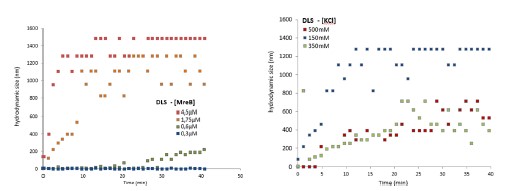
We did not consider these results publishable in the absence of true polymers observed by TEM. As pointed out on the interesting study from Nurse et al. (on E. coli MreB) (Nurse & Marians, 2013), one cannot rely only on light scattering only because non-specific aggregates would show similar patterns than polymers. Over the last two decades, about 15 publications showed polymers of MreB from several Gram-negative species, while none (despite the efforts of many) showed a single convincing MreB polymer from a Gram-positive bacterium by EM. A simple hypothesis is that a critical parameter was missing, and we present convincing evidence that lipids are critical for Geobacillus MreB to form pairs of filaments in the conditions tested. However, in solution too we do occasionally see pairs of filaments (Fig 2-S2), and also sheet-like structures among aggregates when the concentration of MreB is increased (Fig. 2-S2 and Fig. 3-S2). Thus, we agree with the reviewer that it cannot be claimed that Geobacillus MreB is unable to polymerize in the absence of lipids, but rather that lipids strongly stimulate its polymerization, condition depending.
B) The results shown in figure 5A also go against this conclusion, as there is only a 2-fold increase in the phosphate release from MreB(Gs) in the presence of membranes relative to the absence of membranes. Thus, if their model is correct, and MreB(Gs) polymers form only on membranes, this would require the unpolymerized MreB monomers to hydrolyze ATP at 1/2 the rate of MreB in filaments. This high relative rate of hydrolysis of monomers compared to filaments is unprecedented. For all polymers examined so far, the rate of monomer hydrolysis is several orders of magnitude less than that of the filament. For example, actin monomers are known to hydrolyze ATP 430,000X slower than the monomers inside filaments (Blanchoin and Pollard, 2002; Rould et al., 2006).
Response 2.3B. We agree with the reviewer. We have now found conditions where sheets of MreB form in solution (at high MreB concentration) in the presence of ADP and AMP-PNP. However, we have now added several controls that exclude efficient formation of polymers in solution in the presence of ATP at low concentrations of MreBGs (≤ 1.5 µM), the condition used for the malachite green assays. At these MreB concentrations, pairs of filaments are observed in the presence of lipids, but very unfrequently in solution, and sheets are not observed in solution either (Fig. 2-S2A, B). Yet, albeit puzzling, in these conditions Pi release is reproducibly observed in solution, reduced only ~ 2 to 3-fold relative to Pi release in the presence of lipids (Fig. 5A and Fig. 5-S1). A reinforcing observation is when the ATPase assays is performed at 100 mM KCl (Fig. 5A). In this condition MreB binding to lipids is increased relative to 500 mM KCl (Fig. 4-S4C), and the stimulation of the ATPase activity by the presence of lipids is also stronger that at 500 mM (Fig. 5-S1A). Further work is needed to characterize in detail the ATPase activity of MreB proteins, for which data in the literature is very scarce. We can’t exclude that MreB could nucleate in solution or form very unstable filaments that cannot be seen in our EM assay but consume ATP in the process. At the moment, the significance of the Pi released in solution is unknown and will require further investigation.
C) Thus, there is a strong possibility that MreB(Gs) polymers are indeed forming in solution in addition to those on the membrane, and these "solution polymers" may not be captured by their electron microscopy assay. For example, high salt could be interfering with the absorption of filaments to glow discharged lacking lipids.
Response 2.3C. We appreciate the reviewer’s insight about this critical point. Polymers presented in the original Fig. 2A were obtained at 500 mM KCl but we had tested the polymerization of MreB at 100 mM KCl as well, without noticing differences. We have nonetheless redone this quantitatively and used these data for the revised Fig. 2A, as we are now using 100 mM KCl as our standard polymerization condition throughout the revised manuscript. We also followed the other suggestion of the reviewer and tested glow discharged grids (a more classic preparation for soluble proteins) vs non-glow discharged EM grids, as well as a higher concentration of MreB. Grids are generally glow-discharged to make them hydrophilic in order to adsorb soluble proteins, but the properties of MreB (soluble but obviously presenting hydrophobic domains) made difficult to predict what support putative soluble polymers would preferentially interact with. Septins for example bind much better to hydrophobic grids despite their soluble properties (I. Adriaans, personal communication). Virtually no double filaments were observed in solution at either low or high [MreB]. The fact that in some conditions (high [MreB], other nucleotides) we were able to detect sheet-like structures excluded a technical issue that would prevent the detection of existing but “invisible” polymers here. We have added these new data in Fig. 2-S2.
As indicated above, the reviewer’s comments made us realize that we could not state or imply that MreB cannot polymerize in the absence of lipids. As a matter of fact, we always saw some random filaments in the EM fields, both in solution and in the presence of non-hydrolysable analogues, at very low frequency (Fig. 2A). And we do see now sheets at high MreB concentration (Fig. 2-S2B). We could be just missing the optimal conditions for polymerisation in solution, while our phrasing gave the impression that no polymers could ever form in the absence of ATP or lipids. Therefore, we have:
1) analyzed all TEM data to present it as semi-quantitative TEM, using our methodology originally implemented for the analysis of the mutants
2) reworked the text to remove any issuing statements and to indicate that MreBGs was only found to bind to a lipid monolayer as a double protofilament in the presence of ATP/GTP but that this does not exclude that filaments may also form in other conditions.
In order to definitively prove that MreB(Gs) does not have polymers in solution, the authors should:
i) conduct orthogonal experiments to test for polymers in solution. The simplest test of polymerization might be conducting pelleting assays of MreB(Gs) with and without lipids, sweeping through the concentration range as done in 2B and 5a.
Response 2.3Ci. Following reviewer #2 suggestion, we conducted a series of sedimentation assays in the presence and in the absence of lipids, at low (100 mM) and high (500 mM) salt, for both the wild-type protein and the three membrane-anchoring mutants (all at 1.3 µM). Sedimentation experiments in salt conditions preventing aggregation in solution (500 mM KCl) fitted with our TEM results: MreB wild-type pelleting increased in the presence of both ATP and lipids (Fig. R1). The sedimentation was further increased at 100 mM KCl, which would fit our other results indicating an increased interaction of MreB with the membrane. However, in addition to be poorly reproducible (in our hands), the approach does not discriminate between polymers and aggregates (or monomers bound to liposomes) and since MreB has a strong tendency to aggregate, we believe that the technique is ill-suited to reliably address MreB polymerization and prefer not to include sedimentation data in our manuscript. The recent work from Pande et al. (2022) illustrates well this issue since no sedimentation of MreB (at 2 µM) was observed in solution in conditions supporting polymerization (at 300 mM KCl): ‘the protein does not pellet on its own in the absence of liposome, irrespective of its polymerization state’, implying that sedimentation does not allow to detect MreB5 filaments in solution (Pande et al., 2022).
ii) They also could examine if they see MreB filaments in the absence of lipids at 100mM salt (as was seen in both Löwe studies), as the high salt used here might block the charges on glow discharged grids, making it difficult for the polymer to adhere.
See above, Response 2.3C
iii) Likewise, the claim that MreB lacking the amino-terminus and the α2β7 hydrophobic loop "is required for polymerization" is questionable as if deleting these resides blocks membrane binding, the lack of polymers on the membrane on the grid is not unexpected, as these filaments that cannot bind the membrane would not be observable. Given these mutants cannot bind the membrane, mutant polymers could still indeed exist in solution, and thus pelleting assays should be used to test if non-membrane associated filaments composed of these mutants do or do not exist.
Response 2.3Ciii. This is a fair point, we thank the reviewer for this remark. We did not mean to state or imply that the hydrophobic loop was required for polymerization per se, but that polymerization into double filaments only efficiently occurs upon membrane binding, which is mediated by the two hydrophobic sequences. We tested all three mutants by sedimentation as suggested by reviewer #2. In the salt condition that limits aggregation (500 mM KCl) the mutants did not pellet while the wild-type protein did (in the presence of lipids) (Fig. R2 below), in agreement with our EM data. We tested the absence of lipids on the mutant bearing the 2 deletions and observed that the (partial) sedimentation observed at low KCl concentration was ATP and lipid dependent (Fig. R3).
Given our concerns about MreB sedimentation assays (see above, Response 2.3Ci), we prefer not to include these sedimentation data in our manuscript. Instead, we tested by TEM the possible polymerization of the mutants in solution (we only tested them in the presence of lipids in the initial submission). No filaments were detected in solution for any of the mutants (Fig. 4-S3A).
A final note, the results shown in "Figure 1 - figure supplement 2, panel C" appear to directly refute the claim that MreB(Gs) requires lipids to polymerize. As currently written, it appears they can observe MreB(Gs) filaments on EM grids without lipids. If these experiments were done in the presence of lipids, the figure legend should be updated to indicate that. If these experiments were done in the absence of lipids, the claim that membrane association is required for MreB polymerizations should be revised.
The TEM experiments show were indeed performed in the presence of lipids. We apologize for this was not clearly stated in the legend. To prevent all confusion, we have nevertheless removed these images in this figure since the polymerization conditions and lipid requirement are not yet presented when this figure is referred to in the text. We have instead added a panel with the calibration curve for the size exclusion profiles as per request of reviewer #3. The main point of this figure is to show the tendency of MreBGs to aggregate: analytical size-exclusion chromatography shows a single peak corresponding to the monomeric MreBGs, molecular weight ~ 37 KDa, in our purification conditions, but it can readily shift to a peak corresponding to high MW aggregates, depending on the protein concentration and/or storage conditions.
- (Difference 4) - The next difference between this study and previous studies of MreB and actin homologs is the conclusion that MreB(Gs) must hydrolyze ATP in order to polymerize. This conclusion is surprising, given the fact that both T. Maritima (Salje · 2011, Bean 2008) and B. subtilis MreB (Mayer 2009) have been shown to polymerize in the presence of ATP as well as AMP-PNP.
Likewise, MreB polymerization has been shown to lag ATP hydrolysis in not only T. maritima MreB (Esue 2005), eukaryotic actin, and all other prokaryotic actin homologs whose polymerization and phosphate release have been directly compared: MamK (Deng et al., 2016), AlfA (Polka et al., 2009), and two divergent ParM homologs (Garner et al., 2004; Rivera et al., 2011). Currently, the only piece of evidence supporting the idea that MreB(Gs) must hydrolyze ATP in order to polymerize comes from 2 observations: 1) using electron microscopy, they cannot see filaments of MreB(Gs) on membranes in the presence of AMP-PNP or ApCpp, and 2) no appreciable signal increase appears testing AMPPNP- MreB(Gs) using QCM-D. This evidence is by no means conclusive enough to support this bold claim: While their competition experiment does indicate AMPPNP binds to MreB(Gs), it is possible that MreB(Gs) cannot polymerize when bound to AMPPNP.
For example, it has been shown that different actin homologs respond differently to different non-hydrolysable analogs: Some, like actin, can hydrolyze one ATP analog but not the other, while others are able to bind to many different ATP analogs but only polymerize with some of one of them.
Response 2.4. We agree with the reviewer, it is uncertain what analogs bind because they are quite different to ATP and some proteins just do not like them, they can change conditions such that filaments stop forming as well and be (theoretically) misleading. This is why we had tested ApCpp in addition to AMP-PNP as non-hydrolysable analog (Fig. 3A). As indicated above, our new complementary experiments (Fig. 3-S1B-D) now show that some rare (i.e. unfrequently and in limited amount) dual polymers are detected in the presence of ApCpp (Fig. 3A) and at high MreB concentration only in the presence of AMP-PNP (Fig. 3-S1B-D), suggesting different critical concentrations in the presence of alternative nucleotides. We have dampened our conclusions, in the light of our new data, and modified the discussion accordingly.
Thus, to further verify their "hydrolysis is needed for polymerization" conclusion, they should:
A. Test if a hydrolysis deficient MreB(Gs) mutant (such as D158A) is also unable to polymerize by EM.
Response 2.4A. We thank the reviewer for this suggestion. As this conclusion has been reviewed on the basis of our new data (see previous response), testing putative ATPase deficient mutants is no longer required here. The study of ATPase mutants is planned for future studies (see Response 3.10 to reviewer #3).
B. They also should conduct an orthogonal assay of MreB polymerization aside from EM (pelleting assays might be the easiest). They should test if polymers of ATP, AMP-PNP, and MreB(Gs)(D158A) form in solution (without membranes) by conducting pelleting assays. These could also be conducted with and without lipids, thereby also addressing the points noted above in point 3.
Response 2.4B. Please see Response 2.3Ci above.
C. Polymers may indeed form with ATP-gamma-S, and this non-hydrolysable ATP analog should be tested.
Response 2.4C. It is fairly possible that ATP-γ-S supports polymerization since it is known to be partially hydrolysable by actin giving a mild phenotype (Mannherz et al, 1975). This molecule can even be a bona fide substrate for some ATPases (e.g. (Peck & Herschlag, 2003). Thus, we decided to exclude this “non-hydrolysable” analog and tested instead AMP-PNP and ApCpp. We know that ATP-γ-S has been and it is still frequently used, but we preferred to avoid it for the moment for the above-indicated reasons. We chose AMPPNP and AMPPCP instead because (1) they were shown to be completely non-hydrolysable by actin, in contrast to ATP-γ-S; (2) they are widely used (the most commonly used for structural studies; (Lacabanne et al, 2020), (3) AMPPNP was previously used in several publications on MreB (Bean & Amann, 2008; Nurse & Marians, 2013; Pande et al., 2022; Popp et al., 2010; Salje et al, 2011; van den Ent et al., 2014)and thus would allow direct comparison. AMPPCP was added to confirm the finding with AMP-PNP. There are many other analogs that we are planning to explore in future studies (see next Response, 2.4D).
D. They could also test how the ADP-Phosphate bound MreB(Gs) polymerizes in bulk and on membranes, using beryllium phosphate to trap MreB in the ADP-Pi state. This might allow them to further refine their model.
Response 2.4D. We plan to address the question of the transition state in depth in following-up work, using a series of analogs and mutants presumably affected in ATPase activity, both predicted and identified in a genetic screen. As indicated above, it is uncertain what analogs bind because they are quite different to ATP and some may bind but prevent filament formation. Thus, we anticipate that trying just one may not be sufficient, they can change conditions and be (theoretically) misleading and thus a thorough analysis is needed to address this question. Since our model and conclusions have been revised on the basis of our new data, we believe that these experiments are beyond the scope of the current manuscript.
E. Importantly, the Mayer study of B. subtilis MreB found the same results in regard to nucleotides, "In polymerization buffer, MreB produced phosphate in the presence of ATP and GTP, but not in ADP, AMP, GDP or AMP-PNP, or without the readdition of any nucleotide". Thus this paper should be referenced and discussed
Response 2.4E. We agree that Pi release was detected previously. We have added the reference (L121)
- (Difference 5) - The introduction states (lines 128-130) "However, the need for nucleotide binding and hydrolysis in polymerization remains unclear due to conflicting results, in vivo and in vitro, including the ability of MreB to polymerize or not in the presence of ADP or the non-hydrolysable ATP analog AMP-PNP."
A) While this is a great way to introduce the problem, the statement is a bit vague and should be clarified, detaining the conflicting results and appropriate references. For example, what conflicting in vivo results are they referring to? Regarding "MreB polymerization in AMP-PNP", multiple groups have shown the polymerization of MreB(Tm) in the presence of AMP-PNP, but it is not clear what papers found opposing results.
Response 2.5A. Thanks for the comment. We originally did not detail these ‘conflicting results’ in the Introduction because we were doing it later in the text, with the appropriate references, in particular in the Discussion (former L433-442). We have now removed this from the Discussion section and added a sentence in the introduction too (L123-130) quickly detailing the discrepancies and giving the references.
-
For more clarity, we have removed the “in vivo” (which referred to the distinct results reported for the presumed ATPase mutants by the Garner and Graumann groups) and focus on the in vitro discrepancies only.
-
These discrepancies are the following: while some studies showed indeed polymerization (as assessed by EM) of MreBTm in the presence of AMPPNP, the studies from Popp et al and Esue et al on T. maritima MreB, and of Nurse et al on E. coli MreB reported aggregation in the presence of AMP-PNP (Esue et al., 2006; Popp et al., 2010) or ADP (Nurse & Marians, 2013), or no assembly in the presence of ADP (Esue et al., 2006). As for the studies reporting polymerization in the presence of AMP-PNP by light scattering only (Bean & Amann, 2008; Gaballah et al, 2011; Mayer & Amann, 2009; Nurse & Marians, 2013), they could not differentiate between aggregates or true polymers and thus cannot be considered conclusive.
B) The statement "However, the need for nucleotide binding and hydrolysis in polymerization remains unclear due to conflicting results, in vivo and in vitro, including the ability of MreB to polymerize or not in the presence of ADP or the non-hydrolyzable ATP analog AMP-PNP" is technically incorrect and should be rephrased or further tested.
i. For all actin (or tubulin) family proteins, it is not that a given filament "cannot polymerize" in the presence of ADP but rather that the ADP-bound form has a higher critical concentration for polymer formation relative to the ATP-bound form. This means that the ADP polymers can indeed polymerize, but only when the total protein exceeds the ADP critical concentration. For example, many actin-family proteins do indeed polymerize in ADP: ADP actin has a 10-fold higher critical concentration than ATP actin, (Pollard, 1984) and the ADP critical concentrations of AlfA and ParM are 5X and 50X fold higher (respectively) than their ATP-bound forms(Garner et al., 2004; Polka et al., 2009)
Response 2.5Bi. Absolutely correct. We apologize for the lack of accuracy of our phrasing and have corrected it (L123).
ii. Likewise, (Mayer and Amann, 2009) have already demonstrated that B. subtilis MreB can polymerize in the presence of ADP, with a slightly higher critical concentration relative to the ATP-bound form.
Response 2.5Bii. In Mayer and Amann, 2009, the same light scattering signal (interpreted as polymerization) occurred regardless of the nucleotide, and also in the absence of nucleotide (their Fig. 10) and ATP-, ADP- and AMP-PNP-MreB ‘displayed nearly indistinguishable critical concentrations’. They concluded that MreB polymerization is nucleotide-independent. Please see below (responses to ’Other points to address’) our extensive answer to the Mayer & Amann recurring point of reviewer #2
Thus, to prove that MreB(Gs) polymers do not form in the presence of ADP would require one to test a large concentration range of ADP-bound MreB(Gs). They should test if ADP- MreB(Gs) polymerizes at the highest MreB(Gs) concentrations that can be assayed. Even if this fails, it may be the MreB(Gs) ADP polymerizes at higher concentrations than is possible with their protein preps (13uM). An even more simple fix would be to simply state MreB(Gs)-ADP filaments do not form beneath a given MreB(Gs) concentration.
We agree with the reviewer. Our wording was overstating our conclusions. Based on our new quantifications (Fig. 3-S1B, D), we have rephrased the results section and now indicate that pairs of filaments are occasionally observed in the presence of ADP in our conditions across the range of MreB concentration that could be tested, suggesting a higher critical concentration for MreB-ADP (L310-312). Only at the highest MreB concentration, sheet- and ribbon-like structures were observed in the presence of ADP (Fig. 3-S2B).
Other Points to address:
1) There are several points in this paper where the work by Mayer and Amann is ignored, not cited, or readily dismissed as "hampered by aggregation" without any explanation or supporting evidence of that fact.
We have cited the Mayer study where appropriate. However, we cannot cite it as proof of polymerization in such or such condition since their approach does not show that polymers were obtained in their conditions. Again, they based all their conclusions solely on light scattering experiments, which cannot differentiate between polymers and aggregates.
A) Lines 100-101 - While the irregular 3-D formations seen formed by MreB in the Dersch 2020 paper could be interpreted as aggregates, stating that the results from specifically the Gaballah and Meyer papers (and not others) were "hampered by aggregation" is currently an arbitrary statement, with no evidence or backing provided. Overall, these lines (and others in the paper) dismiss these two works without giving any evidence to that point. Thus, they should provide evidence for why they believe all these papers are aggregation, or remove these (and other) dismissive statements.
We apologize if our statements about these reports seemed dismissive or disrespectful, it was definitely not our intention. Light scattering shows an increase of size of particles over time, but there is no way to tell if the scattering is due to organized (polymers) or disorganized (aggregation) assemblies. Thus, it cannot be considered a conclusive evidence of polymerization without the proof that true filaments are formed by the protein in the conditions tested, as confirmed by EM for example. MreB is known to easily aggregate (see our size exclusion chromatography profiles and ones from Dersch 2020 (Dersch et al, 2020), and note that no chromatography profiles were shown in the Mayer report) and, as indicated above, we had similar light scattering results for MreB for years, while only aggregates could be observed by TEM (see above Response 2.3A). Several observations also suggest that aggregation instead of polymerization might be at play in the Mayer study, for example ‘polymerization’ occurring in salt-less buffer but ‘inhibited’ with as low as 100 mM KCl, which should rather be “salting in” (see below). We did not intend to be dismissive, but it seemed wrong to report their conclusions as conclusive evidence. We thought that we had cited these papers where appropriate but then explained that they show no conclusive proof of polymerization and why, but it is evident that we failed at communicating it clearly. We have reworked the text to remove any issuing and arbitrary statement about our concerns regarding these reports (e.g. L93 & L126).
One important note - There are 2 points indicating that dismissing the Meyer and Amann work as aggregation is incorrect:
1) the Meyer work on B. subtilis MreB shows both an ATP and a slightly higher ADP critical concentration. As the emergence of a critical concentration is a steady-state phenomenon arising from the association/dissociation of monomers (and a kinetically limiting nucleation barrier), an emergent critical concentration cannot arise from protein aggregation, critical concentrations only arise from a dynamic equilibrium between monomer and polymer.
- Critical concentration for ATP, ADP or AMPPNP were described in Mayer & Amann (Mayer & Amann, 2009) as “nearly indistinguishable” (see Response 2.5Bii)
- Protein aggregation depends on the solution (pH and ions), protein concentration and temperature. And above a certain concentration, proteins can become instable, thus a critical concentration for aggregation can emerge.
2) Furthermore, Meyer observed that increased salt slowed and reduced B. subtilis MreB light scattering, the opposite of what one would expect if their "polymerization signal" was only protein aggregation, as higher salts should increase the rate of aggregation by increasing the hydrophobic effect.
It is true that at high salt concentration proteins can precipitate, a phenomenon described as “salting out”. However, it is also true that salts help to solubilize proteins (“salting in”), and that proteins tend to precipitate in the absence of salt. Considering that the starting point of the Mayer and Amann experiment (Mayer & Amann, 2009) is the absence of salt (where they observed the highest scattering) and that they gradually reduce this scattering by increasing KCl (the scattering is almost abolished below 100 mM only!) it is plausible that a salting-in phenomenon might be at play, due to increased solubility of MreB by salt. In any case, this cannot be taken as a proof that polymerization rather than aggregation occurred.
B) Lines 113-137 -The authors reference many different studies of MreB, including both MreB on membranes and MreB polymerized in solution (which formed bundles). However, they again neglect to mention or reference the findings of Meyer and Amann (Mayer and Amann, 2009), as it was dismissed as "aggregation". As B. subtilis is also a gram-positive organism, the Meyer results should be discussed.
We did cite the Mayer and Amann paper but, as explained above, we cannot cite this study as an example of proven polymerization. We avoided as much as possible to polemicize in the text and cited this paper when possible. Again, we have reworked the text to avoid any issuing or dismissive statement. Also, we forgot mentioned this study at L121 as an example of reported ATPase activity, and this has now been corrected.
2) Lines 387-391 state the rates of phosphate release relative to past MreB findings: "These rates of Pi release upon ATP hydrolysis (~ 1 Pi/MreB in 6 min at 53{degree sign}C) are comparable to those observed for MreBTm and MreB(Ec) in vitro". While the measurements of Pi release AND ATP hydrolysis have indeed been measured for actin, this statement does not apply to MreB and should be corrected: All MreB papers thus far have only measured Pi release alone, not ATP hydrolysis at the same time. Thus, it is inaccurate to state "rates of Pi release upon ATP hydrolysis" for any MreB study, as to accurately determine the rate of Pi release, one must measure: 1. The rate of polymer over time, 2) the rate of ATP hydrolysis, and 3) the rate of phosphate release. For MreB, no one has, so far, even measured the rates of ATP hydrolysis and phosphate release with the same sample.
We completely agree with the reviewer, we apologize if our formulation was inaccurate. We have corrected the sentence (L479). Thank you for pointing out this mistake.
3) The interpretation of the interactions between monomers in the MreB crystal should be more carefully stated to avoid confusion. While likely not their intention, the discussions of the crystal packing contacts of MreB can appear to assume that the monomer-monomer contacts they see in crystals represent the contacts within actual protofilaments. One cannot automatically assume the observations of monomer-monomer contacts within a crystal reflect those that arise in the actual filament (or protofilament).
We agree, we thank the reviewer for his comments. We have revamped the corresponding paragraph.
A) They state, "the apo form of MreBGs forms less stable protofilaments than its G- homologs ." Given filaments of the Apo form of MreB(GS) or b. subtilis have never been observed in solution, this statement is not accurate: while the contacts in the crystal may change with and without nucleotide, if the protein does not form polymers in solution in the apo state, then there are no "real" apo protofilaments, and any statements about their stability become moot. Thus this statement should be rephrased or appropriately qualified.
see above.
B) Another example: while they may see that in the apo MreB crystal, the loop of domain IB makes a single salt bridge with IIA and none with IIB. This contrasts with every actin, MreB, and actin homolog studied so far, where domain IB interacts with IIB. This might reflect the real contacts of MreB(Gs) in the solution, or it may be simply a crystal-packing artifact. Thus, the authors should be careful in their claims, making it clear to the reader that the contacts in the crystal may not necessarily be present in polymerized filaments.
Again, we agree with the reviewer, we cannot draw general conclusions about the interactions between monomers from the apo form. We have rephrased this paragraph.
4) lines 201-202 - "Polymers were only observed at a concentration of MreB above 0.55 μM (0.02 mg/mL)". Given this concentration dependence of filament formation, which appears the same throughout the paper, the authors could state that 0.55 μM is the critical concentration of MreB on membranes under their buffer conditions. Given the lack of critical concentration measurement in most of the MreB literature, this could be an important point to make in the field.
Following reviewer’s #2 suggestion, we have now estimated the critical concentration (Cc=0.4485 µM) and reported it in the text. (L218).
5) Both mg/ml and uM are used in the text and figures to refer to protein concentration. They should stick to one convention, preferably uM, as is standard in the polymer field.
Sorry for the confusion. We have homogenized to MreB concentrations to µM throughout the text and figures.
6) Lines 77-78 - (Teeffelen et al., 2011) should be referenced as well in regard to cell wall synthesis driving MreB motion.
This has been corrected, sorry for omitting this reference.
7) Line 90 - "Do they exhibit turnover (treadmill) like actin filaments?". This phrase should be modified, as turnover and treadmilling are two very different things. Turnover is the lifetime of monomers in filaments, while treadmilling entails monomer addition at one end and loss at the other. While treadmilling filaments cause turnover, there are also numerous examples of non-treadmilling filaments undergoing turnover: microtubules, intermediate filaments, and ParM. Likewise, an antiparallel filament cannot directionally treadmill, as there is no difference between the two filament ends to confer directional polarity.
This is absolutely true, we apologize for our mistake. The sentence has been corrected (L82).
8) Throughout the paper, the term aggregation is used occasionally to describe the polymerization shown in many previous MreB studies, almost all of which very clearly showed "bundled" filaments, very distinct entities from aggregates, as a bundle of polymers cannot form without the filaments first polymerizing on their own. Evidence to this point, polymerization has been shown to precede the bundling of MreB(Tm) by (Esue et al., 2005).
We agree with reviewer #2 about polymers preceding bundles and “sheets”. However, we respectfully disagree that we used the word aggregation “throughout the paper” to describe structures that clearly showed polymers or sheets of filaments. A search (Ctrl-F: “aggreg”) reveals only 6 matches, 3 describing our own observations (L152, 163/5, and 1023/28), one referring to (Salje et al., 2011) (L107) but citing her claim that they observed aggregation (due to the N-terminus), and the last two (L100, L440) refer (again) to the Gaballah/Mayer/Dersch publications to say that aggregation could not be excluded in these reports as discussed above (Dersch et al., 2020; Gaballah et al., 2011; Mayer & Amann, 2009).
9) lines 106-108 mention that "The N-terminal amphipathic helix of E. coli MreB (MreBEc) was found to be necessary for membrane binding. " This is not accurate, as Salje observed that one single helix could not cause MreB to mind to the membrane, but rather, multiple amphipathic helices were required for membrane association (Salje et al., 2011).
Salje et al showed that in vivo the deletion of the helix abolishes the association of MreB to the membrane. This publication also shows that in vitro, addition of the helix to GFP (not to MreB) prompts binding to lipid vesicles, and that this was increased if there are 2 copies of the helix, but they could not test this directly in vitro with MreB (which is insoluble when expressed with its N-terminus). This prompted them to speculate that multiple MreBs could bind better to the membrane than monomers. However, this remained to be demonstrated. Additional hydrophobic regions in MreB such as the hydrophobic loop could participate to membrane anchoring but are absent in their in vitro assays with GFP.
The Salje results imply that dimers (or further assemblies) of MreB drive membrane association, a point that should be discussed in regard to the question "What prompts the assembly of MreB on the inner leaflet of the cytoplasmic membrane?" posed on lines 86-87.
We agree that this is an interesting point. As it is consistent with our results, we have incorporated it to our model (Fig. 6) and we are addressing it in the discussion L573-575.
10) On lines 414-415, it is stated, "The requirement of the membrane for polymerization is consistent with the observation that MreB polymeric assemblies in vivo are membrane-associated only." While I agree with this hypothesis, it must be noted that the presence or absence of MreB polymers in the cytoplasm has not been directly tested, as short filaments in the cytoplasm would diffuse very quickly, requiring very short exposures (<5ms) to resolve them relative to their rate of diffusion. Thus, cytoplasmic polymers might still exist but have not been tested.
This is also an interesting point. Indeed if a nucleated form, or very short (unbundled) polymers exist in the cytoplasm, they have not been tested by fluorescence microscopy. However, the polymers that localize at the membrane (~ 200 nm), if soluble, would have been detected in the cytoplasm by the work of reviewer #2, us or others.
11) lines 429-431 state, "but polymerization in the presence of ADP was in most cases concluded from light scattering experiments alone, so the possibility that aggregation rather than ordered polymerization occurred in the process cannot be excluded."
A) If an increased light scattering signal is initiated by the addition of ADP (or any nucleotide), that signal must come from polymerization or multimerization. What the authors imply is that there must be some ADP-dependent "aggregation" of MreB, which has not been seen thus far for any polymer. Furthermore, why would the addition of ADP initiate aggregation?
We did not mean that ADP itself would prompt aggregation, but that the protein would aggregate in the buffer regardless of the presence of ADP or other nucleotides. The Mayer & Amann study claims that MreB “polymerization” is nucleotide-independent, as they got identical curves with ATP, ADP, AMPPNP and even with no nucleotides at all (Fig. 10 in their paper, pasted here) (Mayer & Amann, 2009).
Their experiments with KCl are also remarkable as when they lowered the salt they got faster and faster “polymerization”, with the strongest light scattering signal in the absence of any salt. The high KCl concentration in which they got almost no more “polymers” was 75 mM KCl, and ‘polymerization was almost entirely inhibited at 100 mM’ (Fig. 7, pasted below). Yet the intracellular level of KCl in bacteria is estimated to be ~300 mM (see Response 1.1)
B) Likewise, the statement "Differences in the purity of the nucleotide stocks used in these studies could also explain some of the discrepancies" is unexplained and confusing. How could an impurity in a nucleotide stock affect the past MreB results, and what is the precedent for this claim?
We meant that the presence of ATP in the ADP stocks might have affected the outcome of some assays, generating the conflicting results existing in the literature. We agree this sentence was confusing, we have removed it.
12) lines 467-469 state, "Thus, for both MreB and actin, despite hydrolyzing ATP before and after polymerization, respectively, the ADP-Pi-MreB intermediate would be the long-lived intermediate state within the filaments."
A) For MreB, this statement is extremely speculative and unbiased, as no one has measured 1) polymerization, 2) ATP hydrolysis, and 3) phosphate release. For example, it could be that ATP hydrolysis is slow, while phosphate release is fast, as is seen in the actin from Saccharomyces cerevisiae.
We agree that this was too speculative. This has been removed from the (extensively) modified Discussion section. Thanks for the comment.
B) For actin, the statement of hydrolysis of ATP of monomer occurring "before polymerization" is functionally irrelevant, as the rate of ATP hydrolysis of actin monomers is 430,000 times slower than that of actin monomers inside filaments (Blanchoin and Pollard, 2002; Rould et al., 2006).
We agree that the difference of hydrolysis rate between G-actin and F-actin implies that ATP hydrolysis occurs after polymerization. We are afraid that we do not follow the reviewer’s point here, we did not say or imply that ATP hydrolysis by actin monomers was functionally relevant.
13) Lines 442-444. "On the basis of our data and the existing literature, we propose that the requirement for ATP (or GTP) hydrolysis for polymerization may be conserved for most MreBs." Again, this statement both here (and in the prior text) is an extremely bold claim, one that runs contrary to a large amount of past work on not just MreB, but also eukaryotic actin and every actin homolog studied so far. They come to this model based on 1) one piece of suggestive data (the behavior of MreB(GS) bound to 2 non-hydrolysable ATP analogs in 500mM KCL), and 2) the dismissal (throughout the paper) of many peer-reviewed MreB papers that run counter to their model as "aggregation" or "contaminated ATP stocks ." If they want to make this bold claim that their finding invalidates the work of many labs, they must back it up with further validating experiments.
We respectfully disagree that our model was based on “one piece of suggestive data” and backed-up by dismissing most past work in the field. We only wanted to raise awareness about the conflicting data between some reports (listed in response 2.5a), and that the claims made by some publications are to be taken with caution because they only rely on light scattering or, when TEM was performed, showed only disorganized structures.
This said, we clearly failed in proposing our model and we are sorry to see that we really annoyed the reviewer with our suspicion that the work by Mayer & Amann reports aggregation. As indicated above, we have amended our manuscript relative to this point. We also agree that our suggestion to generalize our findings to most MreBs was unsupported, and overstated considering how confusing some result from the literature are. We have refined our model and reworked the text to take on board the reviewer’s remarks as well as the new data generated during the revision process.
We would like to thank reviewer #2 for his in-depth review of our manuscript.
Reviewer #3 (Public Review):
The major claim from the paper is the dependence of two factors that determine the polymerization of MreB from a Gram-positive, thermophilic bacteria 1) The role of nucleotide hydrolysis in driving the polymerization. 2) Lipid bilayer as a facilitator/scaffold that is required for hydrolysis-dependent polymerization. These two conclusions are contrasting with what has been known until now for the MreB proteins that have been characterized in vitro. The experiments performed in the paper do not completely justify these claims as elaborated below.
We understand the reviewer’ concerns in view of the existing literature on actin and Gram-negative MreBs. We may just be missing the optimal conditions for polymerisation in solution, while our phrasing gave the impression that polymers could never form in the absence of ATP or lipids. Our new data actually shows that MreBGs at higher concentration can assemble into bundle- and sheet-like structures in solution and in the presence of ADP/AMP-PNP. Pairs of filaments are however only observed in the presence of lipids for all conditions tested. As indicated in the answers to the global review comments, we have included our new data in the manuscript, revised our conclusions and claims about the lipid requirement and expanded on these points in the Discussion.
Major comments:
1) No observation of filaments in the absence of lipid monolayer can also be accounted due to the higher critical concentration of polymerization for MreBGS in that condition. It is seen that all the negative staining without lipid monolayer condition has been performed at a concentration of 0.05 mg/mL. It is important to check for polymerization of the MreBGS at higher concentration ranges as well, in order to conclusively state the requirement of lipids for polymerization.
Response 3.1. 0.05 mg/ml (1.3µM) is our standard condition, and our leeway was limited by the rapid aggregation observed at higher MreB concentrations, as indicated in the text. We have now tested as well 0.25 mg/ml (6.5 µM - the maximum concentration possible before major aggregation occurs in our experimental conditions). At this higher concentration, we see some sheet-like structures in solution, confirming a requirement of a higher concentration of MreB for polymerization in these conditions (see the answers to the global review comments for more details)
We thank the reviewer for pushing us to address this point. We have revised our conclusions accordingly.
2) The absence of filaments for the non-hydrolysable conditions in the lipid layer could also be because the filaments that might have formed are not binding to the planar lipid layer, and not necessarily because of their inability to polymerize.
Response 3.2. This is a fair point. To test the possibility that polymers would form but would not bind to the lipid layer we have now added additional semi-quantitative EM controls (for both the non-hydrolysable ATP analogs and the three ‘membrane binding’ deletion mutants) testing polymerization in solution (without lipids) and also using plasma-treated grids. These showed that in our standard polymerization conditions, virtually no polymers form in solution (Fig. 3-S1B and Fig. 4-S4A). Albeit at very low frequency, some dual protofilaments were however detected in the presence of ADP or AMP-PNP at the high MreB concentration (Fig. 3-S1D). At this high MreB concentration, the sheet-like structures occasionally observed in solution in the presence of ATP were frequent in the presence of ADP and very frequent in the presence of AMP-PNP (Fig. 3-S2B). We have revised our conclusions on the basis of these new data: MreBGs can form polymeric assemblies in solution and in the absence of ATP hydrolysis at a higher critical concentration than in the presence of ATP and lipids.
See the answers to the global review comments (point 2) and Response 2.3C to reviewer #2 for more details.
3) Given the ATPase activity measurements, it is not very convincing that ATP rather than ADP will be present in the structure. The ATP should have been hydrolysed to ADP within the structure. The structure is now suggestive that MreB is not capable of hydrolysis, which is contradictory to the ATP hydrolysis data.
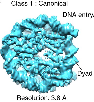
Response 3.3. We thank the reviewer for her insightful remarks about the MreB-ATP crystal structure. The electron density map clearly demonstrates the presence of 3 phosphates. However, as suggested by the reviewer, the density which was attributed to a Mg2+ ion was to be interpreted as a water molecule. The absence of Mg2+ in the crystal could thus explain why the ATP had not been hydrolyzed.
References
Arino J, Ramos J, Sychrova H (2010) Alkali metal cation transport and homeostasis in yeasts. Microbiology and molecular biology reviews 74: 95-120
Bean GJ, Amann KJ (2008) Polymerization properties of the Thermotoga maritima actin MreB: roles of temperature, nucleotides, and ions. Biochemistry 47: 826-835
Cayley S, Lewis BA, Guttman HJ, Record MT, Jr. (1991) Characterization of the cytoplasm of Escherichia coli K-12 as a function of external osmolarity. Implications for protein-DNA interactions in vivo. Journal of molecular biology 222: 281-300
Dersch S, Reimold C, Stoll J, Breddermann H, Heimerl T, Defeu Soufo HJ, Graumann PL (2020) Polymerization of Bacillus subtilis MreB on a lipid membrane reveals lateral co-polymerization of MreB paralogs and strong effects of cations on filament formation. BMC Mol Cell Biol 21: 76
Eisenstadt E (1972) Potassium content during growth and sporulation in Bacillus subtilis. Journal of bacteriology 112: 264-267
Epstein W, Schultz SG (1965) Cation Transport in Escherichia coli: V. Regulation of cation content. J Gen Physiol 49: 221-234
Esue O, Wirtz D, Tseng Y (2006) GTPase activity, structure, and mechanical properties of filaments assembled from bacterial cytoskeleton protein MreB. Journal of bacteriology 188: 968-976
Gaballah A, Kloeckner A, Otten C, Sahl HG, Henrichfreise B (2011) Functional analysis of the cytoskeleton protein MreB from Chlamydophila pneumoniae. PloS one 6: e25129
Harne S, Duret S, Pande V, Bapat M, Beven L, Gayathri P (2020) MreB5 Is a Determinant of Rod-to-Helical Transition in the Cell-Wall-less Bacterium Spiroplasma. Curr Biol 30: 4753-4762 e4757
Kang H, Bradley MJ, McCullough BR, Pierre A, Grintsevich EE, Reisler E, De La Cruz EM (2012) Identification of cation-binding sites on actin that drive polymerization and modulate bending stiffness. Proceedings of the National Academy of Sciences of the United States of America 109: 16923-16927
Lacabanne D, Wiegand T, Wili N, Kozlova MI, Cadalbert R, Klose D, Mulkidjanian AY, Meier BH, Bockmann A (2020) ATP Analogues for Structural Investigations: Case Studies of a DnaB Helicase and an ABC Transporter. Molecules 25
Mannherz HG, Brehme H, Lamp U (1975) Depolymerisation of F-actin to G-actin and its repolymerisation in the presence of analogs of adenosine triphosphate. Eur J Biochem 60: 109-116
Mayer JA, Amann KJ (2009) Assembly properties of the Bacillus subtilis actin, MreB. Cell motility and the cytoskeleton 66: 109-118
Nurse P, Marians KJ (2013) Purification and characterization of Escherichia coli MreB protein. The Journal of biological chemistry 288: 3469-3475
Pande V, Mitra N, Bagde SR, Srinivasan R, Gayathri P (2022) Filament organization of the bacterial actin MreB is dependent on the nucleotide state. The Journal of cell biology 221
Peck ML, Herschlag D (2003) Adenosine 5 '-O-(3-thio)triphosphate (ATP-gamma S) is a substrate for the nucleotide hydrolysis and RNA unwinding activities of eukaryotic translation initiation factor eIF4A. Rna 9: 1180-1187
Popp D, Narita A, Maeda K, Fujisawa T, Ghoshdastider U, Iwasa M, Maeda Y, Robinson RC (2010) Filament structure, organization, and dynamics in MreB sheets. The Journal of biological chemistry 285: 15858-15865
Rhoads DB, Waters FB, Epstein W (1976) Cation transport in Escherichia coli. VIII. Potassium transport mutants. J Gen Physiol 67: 325-341
Rodriguez-Navarro A (2000) Potassium transport in fungi and plants. Biochimica et biophysica acta 1469: 1-30
Salje J, van den Ent F, de Boer P, Lowe J (2011) Direct membrane binding by bacterial actin MreB. Molecular cell 43: 478-487
Schmidt-Nielsen B (1975) Comparative physiology of cellular ion and volume regulation. J Exp Zool 194: 207-219
Szatmari D, Sarkany P, Kocsis B, Nagy T, Miseta A, Barko S, Longauer B, Robinson RC, Nyitrai M (2020) Intracellular ion concentrations and cation-dependent remodelling of bacterial MreB assemblies. Sci Rep-Uk 10
van den Ent F, Izore T, Bharat TA, Johnson CM, Lowe J (2014) Bacterial actin MreB forms antiparallel double filaments. eLife 3: e02634
Whatmore AM, Chudek JA, Reed RH (1990) The Effects of Osmotic Upshock on the Intracellular Solute Pools of Bacillus subtilis. Journal of general microbiology 136: 2527-2535


 Supplementary Experiment Figure 1. EEG results of Supplementary Experiment 1. (a) Mean rating scores of happy intensity related to happy and neutral expressions of faces with awardee or actor/actress identities. (b) ERPs to faces with awardee or actor/actress identities at the frontal electrodes. The voltage topography shows the scalp distribution of the P570 amplitude with the maximum over the central/parietal region. (c) Mean differential P570 amplitudes to happy versus neutral expressions of faces with awardee or actor/actress identities. The voltage topographies illustrate the scalp distribution of the P570 difference waves to happy (vs. neutral) expressions of faces with awardee or actor/actress identities, respectively. Shown are group means (large dots), standard deviation (bars), measures of each individual participant (small dots), and distribution (violin shape) in (a) and (c).
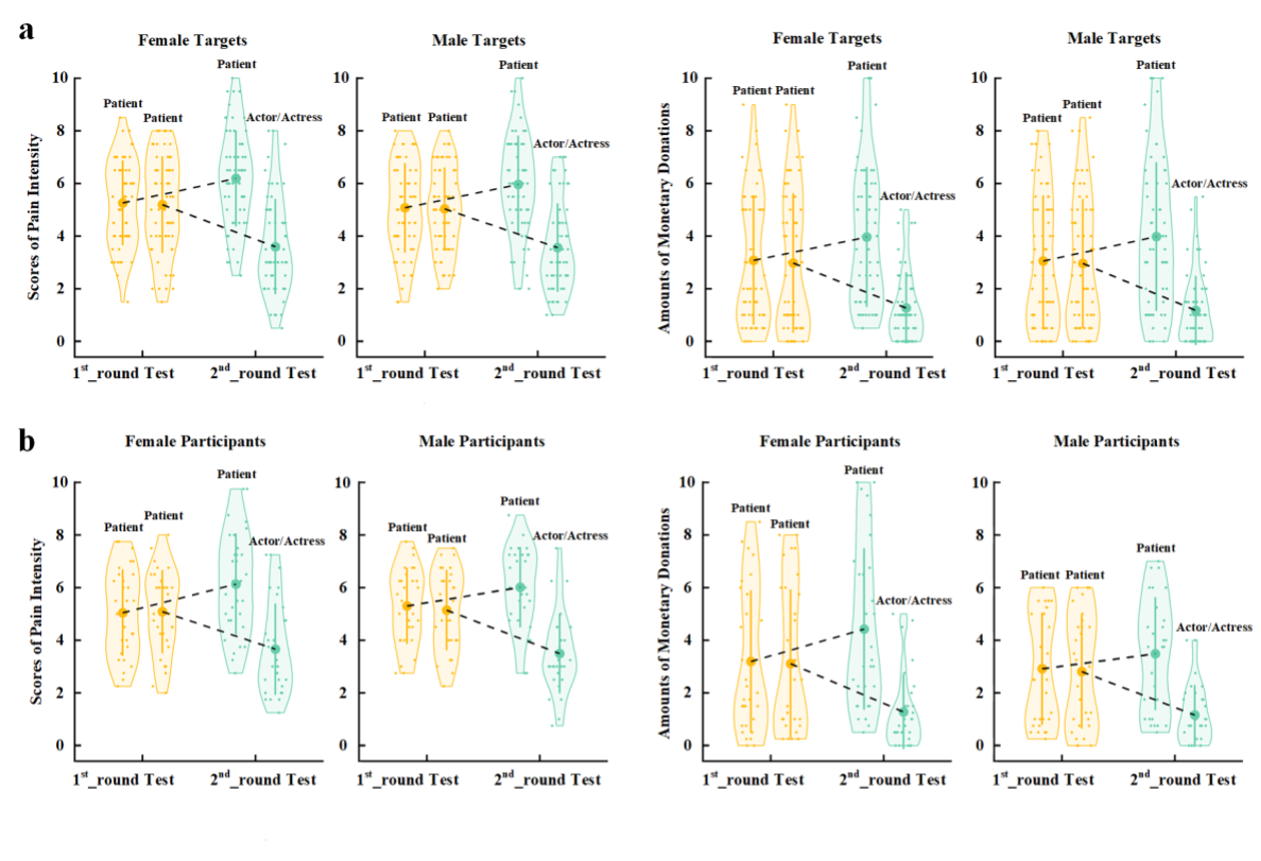 Figure legend: (a) Scores of pain intensity and amount of monetary donations are reported separately for male and female target faces. (b) Scores of pain intensity and amount of monetary donations are reported separately for male and female participants.