Author response:
The following is the authors’ response to the original reviews
eLife Assessment
This study provides a useful analysis of the changes in chromatin organization and gene expression that occur during the differentiation of two cell types (anterior endoderm and prechordal plate) from a common progenitor in zebrafish. Although the findings are consistent with previous work, the evidence presented in the study appears to be incomplete and would benefit from more rigorous interpretation of single-cell data, more in-depth lineage tracing, overexpression experiments with physiological levels of Ripply, and a clearer justification for using an explant system. With these modifications, this paper will be of interest to zebrafish developmental biologists investigating mechanisms underlying differentiation.
We sincerely thank the editor and the reviewers for their valuable time and efforts. Their insightful comments were greatly appreciated and have been largely addressed in the revised manuscript. We are confident that these revisions have enhanced the overall quality and clarity of our paper.
Reviewer #1 (Public review):
Summary:
During vertebrate gastrulation, mesendoderm cells are initially specified by morphogens (e.g. Nodal) and segregate into endoderm and mesoderm in part based on Nodal concentrations. Using zebrafish genetics, live imaging, and single-cell multi-omics, the manuscript by Cheng et al presents evidence to support a claim that anterior endoderm progenitors derive primarily from prechordal plate progenitors, with transcriptional regulators goosecoid (Gsc) and ripply1 playing key roles in this cell fate determination. Such a finding would represent a significant advance in our understanding of how anterior endoderm is specified in vertebrate embryos.
We would like to thank reviewer #1 for his/her comments and positive feedbacks about our manuscript.
Strengths:
Live imaging-based tracking of PP and endo reporters (Figure 2) is well executed and convincing, though a larger number of individual cell tracks will be needed. Currently, only a single cell track (n=1) is provided.
We thank the reviewer for the positive comments and the valuable suggestion. As the reviewer suggested, we re-performed live imaging analyses on the embryos of Tg(gsc:EGFP;sox17:DsRed). We tracked dozens of cells during their transformation from gsc-positive to sox17-positive. Furthermore, we performed quantification of the RFP/GFP signal intensity ratio in these cells over the course of development (Please see the revised Figure 2D and MovieS4).
Weaknesses:
(1) The central claim of the paper - that the anterior endoderm progenitors arise directly from prechordal plate progenitors - is not adequately supported by the evidence presented. This is a claim about cell lineage, which the authors are attempting to support with data from single-cell profiling and genetic manipulations in embryos and explants. The construction of gene expression (pseudo-time) trajectories, while a modern and powerful approach for hypothesis generation, should not be used as a substitute for bona fide lineage tracing methods. If the authors' central hypothesis is correct, a CRE-based lineage tracing experiment (e.g. driving CRE using a PP marker such as Gsc) should be able to label PP progenitor cells that ultimately contribute to anterior endoderm-derived tissues. Such an experiment would also allow the authors to quantify the relative contribution of PP (vs non-PP) cells to the anterior endoderm, which is not possible to estimate from the indirect data currently provided. Note: while the present version of the manuscript does describe a sox17:CRE lineage tracing experiment, this actually goes in the opposite direction that would be informative (sox:17:CRE-marked descendants will be a mixture of PP-derived and non-PP derived cells, and the Gsc-based reporter does not allow for long-term tracking the fates of these cells).
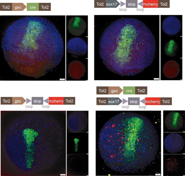
We sincerely thank the reviewer for the professional comments and the constructive suggestions. As the reviewer indicated, utilizing the single-cell transcriptomic trajectory analyses on zebrafish embryos and Nodal-injected explants system, along with the live imaging analyses on Tg(gsc:EGFP;sox17:DsRed) embryos, we revealed that anterior endoderm progenitors arise from prechordal plate progenitors. To further verify this observation, we conducted two sets of lineage-tracing assays. Initial evidence came from the results of co-injecting sox17:Cre and gsc:loxp-STOP-loxp-mcherry plasmids. We observed RFP-positive cells at 8 hpf, demonstrating the presence of cells that had expressed both genes. To explicitly follow the proposed lineage, we then implemented a reciprocal strategy, as suggested by the reviewer, that constructed and co-injected sox17:loxp-STOP-loxp-mcherry and gsc:Cre plasmids. The appearance of RFP-positive cells in the anterior dorsal region at 8 hpf provides direct evidence for a transition from gsc-positive to sox17-positive identity. These results are now included in the revised manuscript (Please see Author response image 1 and Figure S4E). However, in accordance with the reviewer's caution, we acknowledge that this does not prove this is the sole origin of anterior endoderm. Consequently, we have revised the text to clarify that our findings demonstrate that anterior endoderm can be specified from prechordal plate progenitors, without claiming that it is the only source.
Author response image 1.
Characterization of anterior endoderm lineage by Cre-Lox recombination system.
(2) The authors' descriptions of gene expression patterns in the single-cell trajectory analyses do not always match the data. For example, it is stated that goosecoid expression marks progenitor cells that exist prior to a PP vs endo fate bifurcation (e.g. lines 124-130). Yet, in Figure 1C it appears that in fact goosecoid expression largely does not precede (but actually follows) the split and is predominantly expressed in cells that have already been specified into the PP branch. Likewise, most of the cells in the endo branch (or prior) appear to never express Gsc. While these trends do indeed appear to be more muddled in the explant data (Figure 1H), it still seems quite far-fetched to claim that Gsc expression is a hallmark of endoderm-PP progenitors.
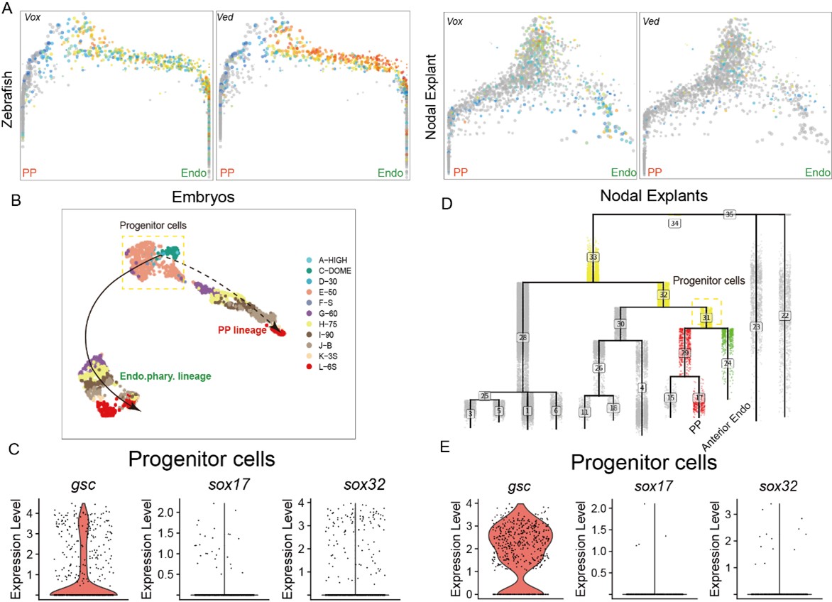
We thank the reviewer for pointing out this issue. Our initial analysis proposed that the precursors of the prechordal plate (PP) and anterior endoderm (endo) more closely resemble a PP cell fate, as their progenitor populations highly express PP marker genes, such as gsc. The gsc gene is widely recognized as a PP marker[1]. The reviewer pointed out that in our analysis, these precursor cells do not initially exhibit high gsc expression; rather, gsc expression gradually increases as PP fate is specified.
The reason for this observation is as follows: First, for the in vivo data, we used the URD algorithm to trace back all possible progenitor cells for both the PP and anterior endo trajectory. As mentioned in the manuscript, the PP and anterior endo are relatively distant in the trajectory tree of the zebrafish embryonic data. Consequently, this approach likely included other, confounding progenitor cells that do not express gsc (like ventral epiblast, Author response image 2). However, we further investigated the expression of gsc and sox17 along these two trajectories. The conclusion remains that gsc expression is indeed higher than sox17 in the progenitor cells common to both trajectories (Author response image 2). Combined with the live imaging analysis presented in this study, which shows that gsc expression increases progressively in the PP, this supports the notion that the progenitor cells for both PP and anterior endoderm initially bias towards a PP cell fate.
On the other hand, in our previously published work using the Nodal-injected explant system, which specifically induces anterior endo and PP, the cellular trajectory analysis also revealed that the specifications of PP and anterior endo follow very similar paths. Therefore, we proceeded to analyze the Nodal explant data. Similarly, when using URD to trace the differentiation trajectories of PP and anterior endo cells, a small number of other progenitor cells were also captured. This explains why a minority of cells do not express gsc—these are likely ventral epiblast cells (Author response image 2). However, based on the Nodal explant data, gsc is specifically highly expressed in the progenitor cells of the PP and anterior endo. Its expression remains high in the PP trajectory but gradually decreases in the endoderm trajectory (Figure 1H).
Author response image 2.
(A) The expression of ventral epiblast markers in PP and anterior Endo URD trajectory. (B) The expression of gsc, sox32 and sox17 in the progenitors of PP and anterior endo in embryos and Nodal explants.
(3) The study seems to refer to "endoderm" and "anterior endoderm" somewhat interchangeably, and this is potentially problematic. Most single-cell-based analyses appearing in the study rely on global endoderm markers (sox17, sox32) which are expressed in endodermal precursors along the entire ventrolateral margin. Some of these cells are adjacent to the prechordal plate on the dorsal side of the gastrula, but many (most in fact) are quite some distance away. The microscopy-based evidence presented in Figure 2 and elsewhere, however, focuses on a small number of sox17-expressing cells that are directly adjacent to, or intermingled with, the prechordal plate. It, therefore, seems problematic for the authors to generalize potential overlaps with the PP lineage to the entire endoderm, which includes cells in ventral locations. It would be helpful if the authors could search for additional markers that might stratify and/or mark the anterior endoderm and perform their trajectory analysis specifically on these cells.
We thank the reviewer for these comments and suggestions. We fully agree with the reviewer's point that the expression of sox32 and sox17 cannot be used to distinguish dorsal endoderm from ventral-lateral endoderm cells. However, during the gastrulation stage, all endodermal cells express sox32 and sox17, and there are currently no specific marker genes available to distinguish between them.
After gastrulation ends, the dorsal endoderm (i.e., the anterior endoderm) begins to express pharyngeal endoderm marker genes, such as pax1b. Therefore, in the analysis of embryonic data in vivo, when studying the segregation of the anterior endoderm and PP trajectory, we specifically used the pharyngeal endoderm as the subject to trace its developmental trajectory.
In the case of Nodal explants, Nodal specifically induces the fate of the dorsal mesendoderm, which includes both the PP and pharyngeal endoderm (anterior endoderm). Precisely for this reason, we consider the Nodal explant system as a highly suitable model for investigating the mechanisms underlying the cell fate separation between anterior endoderm and PP. Thus, in the Nodal explant data, we included all endodermal cells for downstream analysis.
To avoid any potential confusion for readers, we have revised the term "endoderm" in the manuscript to "anterior endoderm" as suggested by the reviewer.
(4) It is not clear that the use of the nodal explant system is allowing for rigorous assessment of endoderm specification. Why are the numbers of endoderm cells so vanishingly few in the nodal explant experiments (Figure 1H, 3H), especially when compared to the embryo itself (e.g. Figures 1C-D)? It seems difficult to perform a rigorous analysis of endoderm specification using this particular model which seems inherently more biased towards PP vs. endoderm than the embryo itself. Why not simply perform nodal pathway manipulations in embryos?
We sincerely thank the reviewer for raising this important question. In our study of the fate separation between the PP and anterior endoderm, we initially analyzed zebrafish embryonic data. However, when reconstructing the transcriptional lineage tree using URD, we observed that these two cell trajectories were positioned relatively far apart on the tree. Yet, existing studies have shown that the anterior endoderm and PP are not only spatially adjacent but also both originate from mesendodermal progenitor cells[2-4], and they share transcriptional similarities[5]. Therefore, as the reviewer pointed out, when tracing all progenitor cells of these two trajectories using the URD algorithm, it is easy to include other cell types, such as ventral epiblast cells (Author response image 2). For this reason, we concluded that directly using embryonic data to dissect the mechanism of fate separation between PP and anterior endoderm might not yield highly accurate results.
In contrast, our group’s previous work, published in Cell Reports, demonstrated that the Nodal-induced explant system specifically enriches dorsal mesendodermal cells, including anterior endoderm, PP, and notochord[5]. Thus, we considered the Nodal explant system to be a highly suitable model for investigating the mechanism of fate separation between PP and anterior endoderm. Ultimately, by analyzing both in vivo embryonic data and Nodal explant data, we consistently found that the anterior endoderm likely originates from PP progenitor cells—a conclusion further validated by live imaging experiments.
Regarding the reviewer’s concern about the relatively low number of endodermal cells in the Nodal explant system, we speculate that this is because the explants predominantly induce anterior endoderm. Since endodermal cells constitute only a small proportion of cells during gastrulation, and anterior endoderm represents an even smaller subset, the absolute number is naturally limited. Nevertheless, the anterior endodermal cells captured in our Nodal explants were sufficient to support our analysis of the fate separation mechanism between anterior endoderm and PP. Finally, to further strengthen the findings from scRNA-seq analyses, we subsequently performed live imaging validation experiments using both zebrafish embryos and the explant system.
(5) The authors should not claim that proximity in UMAP space is an indication of transcriptional similarity (lines 207-208), especially for well-separated clusters. This is a serious misrepresentation of the proper usage of the UMAP algorithm. The authors make a similar claim later on (lines 272-274).
We would like to extend our gratitude to the reviewer for their insightful comments. We have revised the descriptions regarding UMAP throughout the manuscript as suggested (Please see the main text in revised manuscript).
Reviewer # 1 (Recommendations For The Authors):
- Pseudotime trajectories constructed from single-cell snapshots are not true "lineage" measurements. Authors should refrain from referring to such data as lineage data (e.g. lines 99, 100, 103, 109, 112, 127, etc). Such models should be referred to as "trajectories", "hypothetical lineages", or something else.
We are grateful to the reviewer for this comment. Following their recommendation, we have revised the terminology from "transcriptional lineage tree" to "trajectory" across the entire manuscript (Please see main text in revised manuscript).
- The live imaging data presented in Figure 2 (and supplemental figures) are compelling and do seem to show that some cells can switch between PP and endo states. However, the number of cells reported is still too low to be able to ascertain whether or not this is just a rare/edge-case phenomenon. Tracks for just a single cell are reported in Figure 2C-D. This is insufficient. Tracks for many more cells should be collected and reported alongside this current sole (n=1) example. The choice of time window for these live imaging experiments should also be better explained. These live imaging experiments are being performed at or after 6hpf, but authors claim in the text that "... the segregation between PP and Endo has already occurred by 6hpf." (lines 126-127). Why not perform these live imaging experiments earlier, when the initial fate decision between PP and endo is supposedly occurring?
We sincerely appreciate the reviewer’s insightful questions and constructive feedback. In response, we have made several important revisions. First, the reviewer noted that our original manuscript tracked only a single cell and suggested increasing the number of tracked cells. Following this recommendation, we repeated the live-imaging experiments and expanded the number of tracked endodermal cells (Please see the revised Movie S4 and Figure 2D). The experimental conditions were kept identical to the previous setup, and these cells consistently exhibited a gradual transition from a gsc+ fate to a sox17+ endodermal fate. In addition, the reviewer recommended performing live imaging at an earlier time point (Movie S5). Accordingly, we conducted additional experiments initiating live imaging at around 5.7 hours and observed the onset of a sox17 expression in gsc+ cells at approximately 6 hpf, which is consistent with our single-cell transcriptomic analysis.
- The sections devoted to lengthy descriptions of GO terms (lines 131-146, 239-254) and receptor-ligand predictions (lines 170-185) are largely speculative. Consider streamlining.
Thanks for the reviewer's comment. We have streamlined the content related to the GO analysis as suggested (Please see Lines 128-132, 157-167, 221-225).
- The use of a "Nodal Activity Score" (lines 212-226) is clever but might actually be less informative than showing contributions from individual nodal target genes. The combining of counts data from 29 predicted nodal targets means that the contribution (or lack of contribution) from each gene becomes masked. The authors should include supplementary dot plots that break down the score across all 29 genes, allowing the reader to assess overall contributions and/or sub-clusters of gene co-expression patterns, if present.
Thank you very much for the reviewer's positive feedback on our use of the "Nodal Activity Score" and the valuable suggestions provided. Following the recommendation, we analyzed the expression of the 29 Nodal direct targets used in our study across the WT, ndr1 knockdown (kd), and lft1 knockout (ko) groups. We found that the known axial mesoderm genes, such as chrd, tbxta, noto, and gsc, contributed significantly to the Nodal score. The newly conducted analysis has been included in the Supplementary Information (Please see Figure S7L).
- The differential expression trends being reported for srcap (line 251) do not appear to be significant. Are details and P-values for these DEG tests reported somewhere in the manuscript?
We thank the reviewer for raising this question. Based on the reviewer's comment, we performed statistical tests (Wilcoxon test) to compare the expression of srcap in PP and Endo. Our analysis revealed that while srcap expression is slightly higher in PP than in Endo, this difference is not statistically significant. The specific p-value and fold change have been indicated in the revised figure (Please see Figure 4J and S7H). Based on this analysis, we revised our description to state that srcap expression is slightly higher in the PP compared to in the anterior endoderm.
- Following the drug experiments with the drug AU15330 (lines 254-263), authors have only reported #s of endodermal cells, which seem to have increased, which the authors suggest indicates a fate switch from PP to endo. However, the authors have not reported whether the numbers of PP cells decreased or stayed the same in these embryos. This would be helpful information to include, as it is very difficult to discern quantitative trends from the images presented in Fig 4H and 4L.
Thank the reviewer for his/her comments and suggestions. Following the reviewer's suggestions, we performed Imaris analysis on the HCR staining results from the DMSO (control), 1μM AU15330-treated, and 5μM AU15330-treated groups. Our analysis focused on the number of frzb-positive cells (PP), and the comparison revealed that treatment with AU15330 significantly reduces the PP cell number. These findings have been incorporated into the revised manuscript and supplementary information (Please see Figures S7J and S7K).
Reviewer #2 (Public review):
Summary:
During vertebrate gastrulation, the mesoderm and endoderm arise from a common population of precursor cells and are specified by similar signaling events, raising questions as to how these two germ layers are distinguished. Here, Cheng and colleagues use zebrafish gastrulation as a model for mesoderm and endoderm segregation. By reanalyzing published single-cell sequencing data, they identify a common progenitor population for the anterior endoderm and the mesodermal prechordal plate (PP). They find that expression levels of PP genes Gsc and ripply are among the earliest differences between these populations and that their increased expression suppresses the expression of endoderm markers. Further analysis of chromatin accessibility and Ripply cut-and-tag is consistent with direct repression of endoderm by this PP marker. This study demonstrates the roles of Gsc and Ripply in suppressing anterior endoderm fate, but this role for Gsc was already known and the effect of Ripply is limited to a small population of anterior endoderm. The manuscript also focuses extensively on the function of Nodal in specifying and patterning the mesoderm and endoderm, a role that is already well known and to which the current analysis adds little new insight.
We would like to thank the reviewer #2 for the constructive comments and positive feedback regarding our manuscript.
Strengths:
Integrated single-cell ATAC- and RNA-seq convincingly demonstrate changes in chromatin accessibility that may underlie the segregation of mesoderm and endoderm lineages, including Gsc and ripply. Identification of Ripply-occupied genomic regions augments this analysis. The genetic mutants for both genes provide strong evidence for their function in anterior mesendoderm development, although these phenotypes are subtle.
We thank the reviewer for recognizing our work, and we greatly appreciate the constructive suggestions from the reviewer.
Weaknesses:
The use of zebrafish embryonic explants for cell fate trajectory analysis (rather than intact embryos) is not justified. In both transcriptomic comparisons between the two fate trajectories of interest and Ripply cut-and-tag analysis, the authors rely too heavily on gene ontology which adds little to our functional understanding. Much of the work is focused on the role of Nodal in the mesoderm/endoderm fate decision, but the results largely confirm previous studies and again provide few new insights. Some experiments were designed to test the relationship between the mesoderm and endoderm lineages and the role of epigenetic regulators therein, but these experiments were not properly controlled and therefore difficult to interpret.
We sincerely thank the reviewer for the comments. As we previously answered, in our study of the fate differentiation between the PP and the anterior endoderm, we initially analyzed zebrafish embryonic data. However, when we used URD to reconstruct the transcriptional trajectory tree, we found that these two cell trajectories were distantly located on the tree. Existing studies have shown that the anterior endoderm and the PP are not only spatially adjacent but also both originate from mesendodermal progenitor cells and share transcriptional similarities[2-4]. Therefore, when tracing all progenitor cells of these two trajectories using the URD algorithm, it is easy to include other cell types, such as ventral mesendodermal cells (Please see Author response image 2A). Based on this, we believe that directly using embryonic data to decipher the mechanism of fate differentiation between the PP and the anterior endoderm may not yield sufficiently precise results. In contrast, our group’s previous study published in Cell Reports demonstrated that the Nodal-induced explant system can specifically enrich dorsal mesendodermal cells, including the anterior endoderm, PP, and notochord[5]. Thus, we consider the Nodal explant system as an ideal model for studying the fate differentiation mechanism between the PP and the anterior endoderm. Ultimately, through comprehensive analysis of in vivo embryonic data and Nodal explant data, we consistently found that the anterior endoderm likely originates from PP progenitor cells—a conclusion further validated by live imaging experiments.
Regarding the GO analysis, we have streamlined it as suggested by the reviewers. In the revised manuscript, we analyzed the expression of specific genes contributing to key GO functions. Additionally, in the revised version, we conducted more live imaging experiments and quantitative cell assays. We designed gRNA for srcap using the CRISPR CAS13 system to knock down srcap, which further corroborated the morpholino knockdown results, showing consistency with the morpholino data. We also performed Western blot validation of the SWI/SNF complex's response to the drug AU15330, confirming the drug's effectiveness. We hope these additional experiments adequately address the reviewers' concerns.
Reviewer #2 (Recommendations For The Authors):
(1) In the introduction, the authors state that mesendoderm segregates into mesoderm and endoderm in a Nodal-concentration dependent manner. While it is true that higher Nodal signaling levels are required for endoderm specification, A) this is also true for some mesoderm populations, and B) Work from Caroline Hill's lab has shown that Nodal activity alone is not determinative of endoderm fate. Although the authors cite this work, it is conclusions are not reflected in this over-simplified explanation of mesendoderm development. The authors also state that it is not clear when PP and endoderm can be distinguished transcriptionally, but this was also addressed in Economou et al, 2022, which found that they can be distinguished at 60% epiboly but not 50% epiboly.
We sincerely thank the reviewer for raising this question and reminding us of the conclusions drawn from that excellent study. As the reviewer pointed out, Economou et al. demonstrated that Nodal signaling alone is insufficient to determine the cell fate segregation of mesendoderm[6]. However, their study primarily focused on the fate segregation of the ventral-lateral mesendoderm lineage. In contrast, we believe that the mechanisms underlying dorsal mesendoderm specification may differ.
First, it is well-studied that in zebrafish embryos, the most dorsal mesendoderm is initially specified by the activity of the dorsal organizer. Notably, the Nodal signaling ligands ndr1 and ndr2 begin to be expressed in the dorsal organizer as early as the sphere stage[7]. In our study, through single-cell transcriptomic trajectory analysis and live imaging analysis, we observed that the cell fate segregation of the dorsal mesendoderm can be traced back to the shield stage.
Second, the regulatory mechanisms governing dorsal mesendoderm fate differentiation may differ from those of the ventral-lateral mesendoderm. For instance, the gsc gene is exclusively expressed in the dorsal mesendoderm and is absent in the ventral-lateral mesendoderm. Given that gsc is a critical master gene, its overexpression in the ventral side can induce a complete secondary body axis. Similarly, ripply1, identified in our study, is also expressed early and specifically in the dorsal mesendoderm. Overexpression of ripply1 in the ventral side similarly induces a secondary body axis, albeit with the absence of the forebrain[5]. In this study, we found that gsc and ripply1 as the repressor, collectively inhibited dorsal (anterior) endoderm specified from PP progenitors.
In summary, our study focuses on the regulatory mechanisms of fate segregation in the dorsal (anterior) mesendoderm, which differs from the mechanisms of ventral-lateral mesendoderm lineage segregation reported by Economou et al. We believe that this distinction represents a key novelty of our work.
(2) As noted in the manuscript, Warga and Nusslein-Volhard determined long ago that PP and anterior endoderm share a common precursor. It is surprising that this close relationship is not apparent from the lineage trees in whole embryos but is apparent in lineage trees from explants. The authors speculate that the resolution of the whole embryo dataset is insufficient to detect this branch point and propose explants as the solution, but it is not clear why the explant dataset is higher resolution and/or more appropriate to address this question.
We sincerely thank the reviewer for their thoughtful comments. As we mentioned previously, our investigation of fate differentiation between the PP and the anterior endoderm initially involved the analysis of zebrafish embryonic data. However, when we used URD to reconstruct the transcriptional trajectory tree, we observed that these two cell trajectories were located far apart. Previous elegant studies, as the reviewer mentioned, have shown that the anterior endoderm and the PP are not only spatially adjacent but also both originate from mesendodermal progenitor cells and share transcriptional similarities[2,3,8]. Consequently, when tracing all progenitor cells of these two trajectories using the URD algorithm, other cell types—such as ventral mesendodermal cells—are easily included. Based on this, we believe that directly using embryonic data to elucidate the mechanism of fate differentiation between the PP and the anterior endoderm may lack sufficient precision.
In contrast, our group’s previous study published in Cell Reports demonstrated that the Nodal-induced explant system specifically enriches dorsal mesendodermal cells, including the anterior endoderm, PP, and notochord[5]. Therefore, we consider the Nodal explant system as an ideal model for studying the mechanism underlying fate differentiation between the PP and the anterior endoderm. Through comprehensive analyses of both in vivo embryonic and Nodal explant data, we consistently found that the anterior endoderm likely originates from PP progenitor cells—a conclusion further supported by live imaging experiments.
(3) Much of the analysis of DEGs between the lineages of interest is focused on GO term enrichment. But this logic is circular. The endoderm lineage is defined as such because it expresses endoderm-enriched genes, therefore the finding that the endoderm lineage is enriched for endoderm-related GO terms adds no new insights.
We thank the reviewer for these comments. As the reviewers suggested, in the revised manuscript, we indicated specific genes associated with key GO terms (Please see Figure 4B). Additionally, we have streamlined the content related to the GO analysis as suggested.
(4) The authors describe the experiment in Figure S4 as key evidence that Gsc+ cells can give rise to endoderm, but no controls are presented. Only a few cells are shown that express mCherry upon injection of sox17:cre constructs. Is mCherry also expressed in the occasional cell injected with Gsc:lox-stop-lox-mCherry in the absence of cre? Although they report 3 independent replicates, it appears that only 2 individual embryos express mCherry. This very small number is not convincing, especially in the absence of appropriate controls.
We thank the reviewer for raising this question. Following the reviewer's suggestion, we injected gsc:loxp-stop-loxp-mCherry into zebrafish embryos at the 1-cell stage as a control. After performing at least three independent replicates and analyzing no fewer than 100 embryos, we did not observe any mCherry-positive cells. Additionally, we co-injected gsc:loxp-stop-loxp-mCherry with sox17:cre and increased the sample size. Furthermore, we constructed plasmids of sox17:loxp-stop-loxp-mCherry and gsc:cre, and upon injection at the 1-cell stage, we observed RFP-positive cells at 8 hpf (Please see Author response image 1 and Figure S4E). Together with our live imaging data, these experiments collectively demonstrate that anterior endodermal cells can originate from PP progenitors.
(5) The authors spend a lot of effort demonstrating that PP and anterior endoderm are Nodal dependent. First, these data (especially Figures 3E and 3I) are not very convincing, as the differences shown are very small or not apparent. Second, this is already well-known and adds nothing to our understanding of mesoderm-endoderm segregation.
We sincerely thank the reviewer for their insightful questions. First, the reviewer mentioned that in the initial version of our manuscript, the effects of ndr1 knockdown and lefty1 knockout on Nodal signaling and cell fate—particularly prechordal plate (PP) and anterior endoderm (endo)—in Nodal-induced explants were not very pronounced. We recognize that the negative feedback mechanism between Nodal and Lefty signaling may explain why Nodal acts as a morphogen, regulating pattern formation through a Turing-like model[9]. Therefore, knocking down a Nodal ligand gene, such as ndr1 in this study, or knocking out a Nodal inhibitor, such as lft1, may only have a subtle impact on Nodal signaling[10].
Accordingly, in this study, we performed extensive pSmad2 immunofluorescence analysis and observed that although the overall intensity of Nodal activity did not change dramatically, there was a statistically significant difference. Importantly, this subtle variation in Nodal signaling strength is precisely what we intended to capture, since PP and anterior endoderm are highly sensitive to Nodal signaling[11], and even minor differences may bias their fate segregation.
This leads directly to the reviewer’s second concern. While numerous studies suggest that the strength of Nodal signaling influences mesendodermal fate—with high Nodal promoting endoderm and lower concentrations inducing mesoderm—most of these studies focus on ventral-lateral mesendoderm development[4,6,10]. In contrast, the mechanisms underlying dorsal mesendoderm fate specification differ, which is a key innovation of our study.
Previous work by Bernard Thisse and colleagues demonstrated that even a slight reduction in Nodal signaling, achieved by overexpressing a Nodal inhibitor, is sufficient to cause defects in the specification of PP and endoderm[11]. This indicates that PP and endoderm require the highest levels of Nodal signaling for proper specification. Moreover, the most dorsal mesendoderm, PP and anterior endoderm are not only spatially adjacent but also share similar transcriptional states, making the regulation of their fate separation particularly challenging to study.
The Dr. C.P. lab made important contributions to this issue, showing that the duration of Nodal exposure is critical for segregating PP and anterior endoderm fates: prolonged Nodal signaling promotes expression of the transcriptional repressor Gsc, which directly suppresses the key endodermal transcription factor Sox17, thereby inhibiting anterior endoderm specification[3]. They also found that tight junctions among PP cells facilitate Nodal signal propagation[8]. However, their studies revealed that Gsc mutants do not exhibit endodermal phenotypes, suggesting that additional factors or mechanisms regulate PP versus anterior endoderm fate separation[3].
In our study, we first observed that subtle differences in Nodal concentration may bias the fate choice between PP and anterior endoderm. Given that ndr1 knockdown and lft1 knockout mildly reduce or enhance Nodal signaling, respectively, we reasoned that using these two perturbations in a Nodal-induced explant system combined with single-cell RNA sequencing could generate transcriptomic profiles under slightly reduced and enhanced Nodal signaling. This approach may help identify key decision points and transcriptional differences during PP and anterior endoderm segregation, ultimately uncovering the molecular mechanisms downstream of Nodal that govern their fate separation.
(6) The authors claim that scrap expression differs between the 2 lineages of interest, but this is not apparent from Figure 4J-K. Experiments testing the role of SWI/SNF and scrap also require additional controls. Can scrap MO phenotypes be rescued by scrap RNA? Is there validation that SWI/SNF components are degraded upon treatment with AU15330?
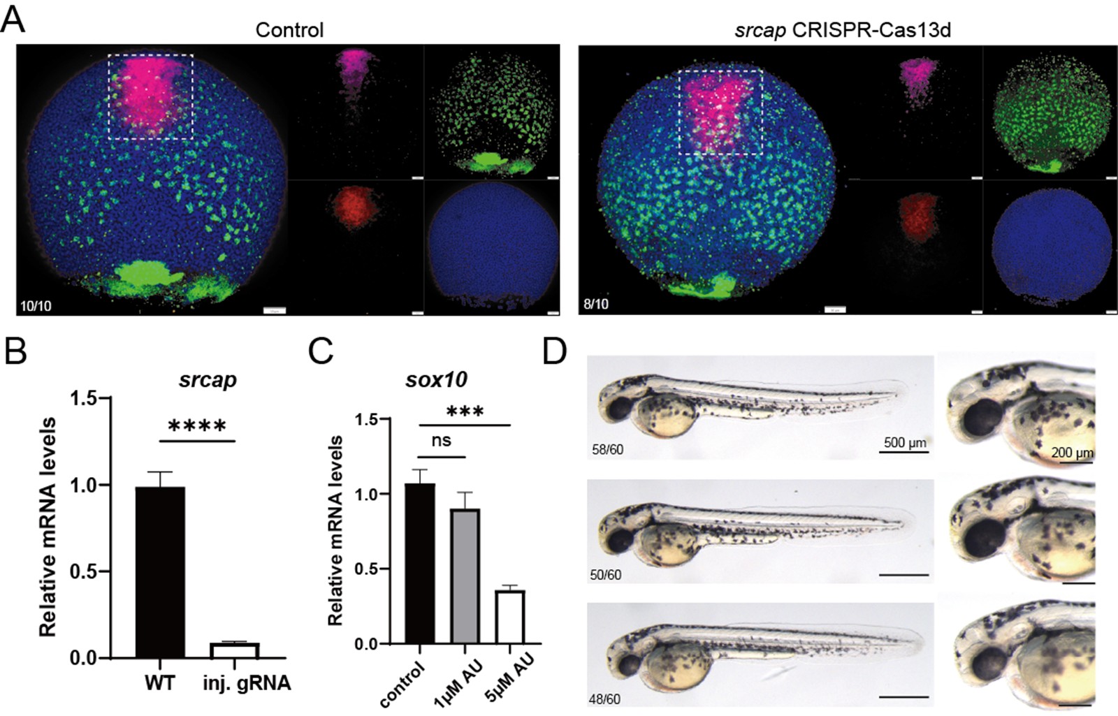
We are very grateful for the reviewers' questions. Using single-cell data from zebrafish embryos and Nodal explants, we compared the expression of srcap in the PP and anterior Endo cell populations. We found that srcap expression showed a slight increase in PP compared to anterior Endo, but the difference was not statistically significant (Please see Figure 4J and S7H). Therefore, we modified our description in the revised manuscript. However, we speculate that this slight difference might influence the distinct cell fate specification between PP and anterior endo. In the original version of the manuscript, we reported that either treatment with AU15330, an inhibitor of the SWI/SNF complex, or injection of morpholino targeting srcap—a key component of the SWI/SNF complex—enhanced anterior endo fate while reducing PP cell specification. During this round of revision, we initially attempted to follow the reviewer’s suggestion to co-inject srcap mRNA along with srcap morpholino to rescue the phenotype. However, we found that the length of srcap mRNA exceeds 10,000 bp, and despite multiple attempts, we were unable to successfully obtain the srcap mRNA. Therefore, we were unable to perform the rescue experiment and instead adopted an alternative approach to validate the function of srcap. We aimed to use anthor knockdown approach (CRISPR/Cas system) to determine whether a phenotype similar to that observed with morpholino knockdown could be achieved. Using the CRISPR/Cas13 system, we designed gRNA targeting srcap, knocked down srcap, and examined the cell specification of PP and anterior endo. We found that, consistent with our previous results, knocking down srcap obviously reduced PP cell fate while increasing anterior endo cell fate (Author response image 3). Additionally, the reviewer raised the question of whether the SWI/SNF complex is degraded after AU15330 treatment. Following the reviewer’s suggestion, we attempted to perform Western blot analysis on BRG1, one of the components of the SWI/SNF complex. However, despite multiple attempts, we were unable to achieve successful detection of the BRG1 protein by the antibody in zebrafish. Several studies have reported that knockdown or knockout of brg1 leads to defects in neural crest cell specification in zebrafish[12,13]. Therefore, alternatively, we treated zebrafish embryos at the one-cell stage with 0 μM (DMSO), 1 μM, and 5 μM AU15330, and examined the expression of sox10 and pigment development around 48 h. We found that treatment with 1 μM AU15330 reduced sox10 expression and pigment production, though not significantly, whereas treatment with 5 μM AU15330 significantly disrupted neural crest cell development. Thus, this experiment demonstrates that AU15330 is functional in zebrafish. (Author response image 3).
Author response image 3.
(A) Characterization of anterior endoderm and PP cells following CRISPR-Cas13d-mediated srcap knockdown. (B) Validation of srcap mRNA expression by RT‑qPCR following CRISPR‑Cas13d knockdown. (C) RT‑qPCR shows the expression of sox10 after treatment with increasing concentrations of AU15300. (D) Morphology of zebrafish embryos at 48 hpf after treatment with increasing concentrations of AU15300.
(7) The authors conclude from their chromatin accessibility analysis that variations in Nodal signaling are responsible for expression levels of PP and endoderm genes, but they do not consider the alternative explanation that FGF signaling is playing this role. Such a function for FGF was established by Caroline Hill's lab, and the authors also show in Figure S5G that FGF signaling in enriched between these cell populations.
Thank you very much for raising this issue. As the reviewer pointed out, Caroline Hill's lab has conducted elegant work demonstrating that FGF signaling plays a crucial role in the separation of ventral-lateral mesendoderm cell fates[4,6]. In contrast, our study primarily focuses on studying the mechanisms underlying the separation of dorsal mesendoderm cell fates. However, our research also reveals that FGF signaling significantly regulates the fate separation of the dorsal mesendoderm, as inhibiting FGF signaling suppresses PP cell specification while promoting anterior Endo fate. In our previously published work, we found that Nodal signaling can directly activate the expression of FGF ligand genes[5]. Therefore, we hypothesize that Nodal signaling, acting as a master regulator, activates various downstream target genes—including FGF—and how FGF signaling regulates the cell fate separation of the dorsal mesendoderm warrants further investigation in our further studies.
(8) When interpreting the results of their Ripply cut-and-run experiment, the authors again rely heavily on GO term analysis and claim that this supports a role for Ripply as a transcriptional repressor. GO term enrichment does not equal functional analysis. It would be more convincing to intersect DEGs between WT and ripply-/- embryos with Ripply-enriched loci.
Thanks for raising this important issue and the constructive suggestion. In response to the reviewer's valid concern regarding the GO term analyses from our CUT&Tag data, we implemented a more stringent filtering strategy. We identified peaks enriched in the treatment group and applied differential analysis, selecting genes with a log<sub>2</sub>FoldChange > 3, padj < 0.05, and baseMean > 30 as high-confidence Ripply1 binding targets. A GO enrichment analysis of these genes revealed significant terms related to muscle development, consistent with Ripply1's established role in somite development, thereby validating our approach. We supplemented the related gene list in the revised manuscript. Moreover, within this refined analysis, we found that sox32 met our binding threshold, while sox17 did not. Furthermore, as suggested, we examined mespbb—a known Ripply1-repressed gene—which was present, and gsc, a Nodal target used as a negative control, which was absent. This confirms the specificity of our analysis (Figure 6 and Figure S11). Consequently, our revised analyses support a model in which Ripply1 directly binds the sox32 promoter. Given that Sox32 is a known upstream regulator of sox17, this binding provides a plausible direct mechanism for the observed regulation of sox17 expression. We have updated the figures and text accordingly. We attempted to generate ripply1<sup>-/-</sup> mutants but found that homozygous loss results in embryonic lethality.
(9) The way N's are reported is unconventional. N= number of embryos used in the experiment, n= number of embryos imaged. If an embryo was not imaged or analyzed in any way, it cannot be considered among the embryos in an experiment. If only 4 embryos were imaged, the N for that experiment is 4 regardless of how many embryos were stained. Authors should also report not only the number of embryos examined but also the number of independent trials performed for all experiments.
Thank you very much for the reviewer's suggestion. As suggested, we have revised the description regarding the number of embryos and experimental replicates in the figure legends.
(10) The authors should avoid the use of red-green color schemes in figures to ensure accessibility for color-blind readers.
Thanks for the suggestions. We have updated the figures in our revised manuscript and adjusted the color schemes to avoid red-green combinations.
Reviewer #3 (Public Review):
Summary:
Cheng, Liu, Dong, et al. demonstrate that anterior endoderm cells can arise from prechordal plate progenitors, which is suggested by pseudo time reanalysis of published scRNAseq data, pseudo time analysis of new scRNAseq data generated from Nodal-stimulated explants, live imaging from sox17:DsRed and Gsc:eGFP transgenics, fluorescent in situ hybridization, and a Cre/Lox system. Early fate mapping studies already suggested that progenitors at the dorsal margin give rise to both of these cell types (Warga) and live imaging from the Heisenberg lab (Sako 2016, Barone 2017) also pretty convincingly showed this. However, the data presented for this point are very nice, and the additional experiments in this manuscript, however, further cement this result. Though better demonstrated by previous work (Alexander 1999, Gritsman 1999, Gritsman 2000, Sako 2016, Rogers 2017, others), the manuscript suggests that high Nodal signaling is required for both cell types, and shows preliminary data that suggests that FGF signaling may also be important in their segregation. The manuscript also presents new single-cell RNAseq data from Nodal-stimulated explants with increased (lft1 KO) or decreased (ndr1 KD) Nodal signaling and multi-omic ATAC+scRNAseq data from wild-type 6 hpf embryos but draws relatively few conclusions from these data. Lastly, the manuscript presents data that SWI/SNF remodelers and Ripply1 may be involved in the anterior endoderm - prechordal plate decision, but these data are less convincing. The SWI/SNF remodeler experiments are unconvincing because the demonstration that these factors are differentially expressed or active between the two cell types is weak. The Ripply1 gain-of-function experiments are unconvincing because they are based on incredibly high overexpression of ripply1 (500 pg or 1000 pg) that generates a phenotype that is not in line with previously demonstrated overexpression studies (with phenotypes from 10-20x lower expression). Similarly, the cut-and-tag data seems low quality and like it doesn't support direct binding of ripply1 to these loci.
In the end, this study provides new details that are likely important in the cell fate decision between the prechordal plate and anterior endoderm; however, it is unclear how Nodal signaling, FGF signaling, and elements of the gene regulatory network (including Gsc, possibly ripply1, and other factors) interact to make the decision. I suggest that this manuscript is of most interest to Nodal signaling or zebrafish germ layer patterning afficionados. While it provides new datasets and observations, it does not weave these into a convincing story to provide a major advance in our understanding of the specification of these cell types.
We sincerely thank the reviewer for their thorough and thoughtful assessment of our work. The reviewer acknowledged several strengths of our study, such as the use of multiple technical approaches to demonstrate that anterior endoderm differentiates from PP progenitor cells, and recognized the value of the newly added single-cell omics data. The reviewer also raised some concerns regarding the initial version of our work, including the SWI/SNF remodeler experiments and the Ripply1 gain-of-function experiment. In the revised manuscript, we have supplemented these parts with additional control experiments to better support our conclusions. We hope that our updated manuscript adequately addresses the points raised by the reviewer.
Major issues:
(1) UMAPs: There are several instances in the manuscript where UMAPs are used incorrectly as support for statements about how transcriptionally similar two populations are. UMAP is a stochastic, non-linear projection for visualization - distances in UMAP cannot be used to determine how transcriptionally similar or dissimilar two groups are. In order to make conclusions about how transcriptionally similar two populations are requires performing calculations either in the gene expression space, or in a linear dimensional reduction space (e.g. PCA, keeping in mind that this will only consider the subset of genes used as input into the PCA). Please correct or remove these instances, which include (but are not limited to):
p.4 107-110
p.4 112
p.8 207-208
p.10 273-275
We would like to thank the reviewer for raising this question. The descriptions of UMAP have been revised throughout the manuscript in accordance with the reviewer's suggestion (Please see the main text in the revised manuscript).
(2) Nodal and lefty manipulations: The section "Nodal-Lefty regulatory loop is needed for PP and anterior Endo fate specification" and Figure 3 do not draw any significant conclusions. This section presents a LIANA analysis to determine the signals that might be important between prechordal plate and endoderm, but despite the fact that it suggests that BMP, Nodal, FGF, and Wnt signaling might be important, the manuscript just concludes that Nodal signaling is important. Perhaps this is because the conclusion that Nodal signaling is required for the specification of these cell types has been demonstrated in zebrafish in several other studies with more convincing experiments (Alexander 1999, Gritsman 1999, Gritsman 2000, Rogers 2017, Sako 2016). While FGF has recently been demonstrated to be a key player in the stochastic decision to adopt endodermal fate in lateral endoderm (Economou 2022), the idea that FGF signaling may be a key player in the differentiation of these two cell types has strangely been relegated to the discussion and supplement. Lastly, the manuscript does not make clear the advantage of performing experiments to explore the PP-Endo decision in Nodal-stimulated explants compared to data from intact embryos. What would be learned from this and not from an embryo? Since Nodal signaling stimulates the expression of Wnts and FGFs, these data do not test Nodal signaling independent of the other pathways. It is unclear why this artificial system that has some disadvantages is used since the manuscript does not make clear any advantages that it might have had.
We sincerely thank the reviewers for their valuable comments. As mentioned in our manuscript, although a substantial number of studies have reported on the mechanisms governing the segregation of mesendoderm fate in zebrafish embryos—including the Dr. Hill laboratory’s work cited by the reviewers, which demonstrated the involvement of FGF signaling in the ventral mesendoderm fate specification—research on the regulatory mechanisms underlying anterior mesendoderm differentiation remains relatively limited. This is largely due to the challenges posed by the close physical proximity and similar transcriptional states of anterior mesendoderm cells, as well as their shared dependence on high levels of Nodal signaling for specification.
Several studies from the Dr. C.P. Heisenberg’s laboratory have attempted to elucidate the fate segregation between anterior mesendoderm cells, namely the prechordal plate (PP) and anterior endoderm (endo) cells. They found that PP cells are tightly connected, facilitating the propagation of Nodal signaling[8]. Prolonged exposure to Nodal activates the expression of Gsc, which acts as a transcriptional repressor to inhibit sox17 expression, thereby suppressing endodermal fate[3]. However, they also noted that Gsc mutants do not exhibit endoderm developmental defects, suggesting the involvement of additional factors in this process.
The reviewer inquired about our rationale for using the Nodal-injected explant system. In our investigation of the fate separation between the PP and the anterior endo, we initially analyzed zebrafish embryonic data. Using URD to reconstruct the transcriptional lineage tree, we found that these two cell types were positioned distantly from each other. However, existing literature indicates that the anterior endoderm and PP are not only spatially adjacent but also derive from common mesendodermal progenitors and exhibit transcriptional similarities[2,8]. As the reviewer noted, when tracing all progenitor cells of these two lineages using URD, it is easy to inadvertently include other cell types—such as ventral epiblast cells—which may compromise the accuracy of the analysis. We therefore concluded that directly using embryonic data to dissect the mechanism of fate separation between PP and anterior endoderm might not yield highly precise results.
By contrast, our group’s earlier study published in Cell Reports demonstrated that the Nodal-induced explant system specifically enriches dorsal mesendodermal cells, including anterior endo, PP, and notochord[5]. This makes the Nodal explant system a highly suitable model for studying the fate separation between PP and anterior endo. Ultimately, by analysing in vivo embryonic data and Nodal explant data, we consistently found that the anterior endoderm likely originates from PP progenitors—a conclusion further supported by live imaging experiments.
As we answered above, we first used the analyses of single-cell RNA sequencing and live imaging to demonstrate that anterior endoderm can originate from PP progenitor cells. Understanding the mechanism underlying the fate segregation between these two cell populations became a key focus of our research. We began by applying cell communication analysis to our single-cell data to identify signaling pathways that may be involved. This analysis specifically highlighted the Nodal-Lefty signaling pathway. Since Lefty acts as an inhibitor of Nodal signaling, we hypothesized that differences in Nodal signaling strength might regulate the fate of these two cell populations. By overexpressing different concentrations of Nodal mRNA and examining the fates of PP and anterior Endo cells, we confirmed this hypothesis.
Thus, we propose that even subtle differences in Nodal signaling levels may influence anterior mesendoderm fate decisions. To test this, we generated systems with slightly reduced Nodal signaling (via ndr1 knockdown) and slightly elevated Nodal signaling (via lft1 knockout). Using these models, we precisely captured the critical stage of fate segregation between PP and anterior endo cells and identified a novel transcriptional repressor, Ripply1, which works in concert with Gsc to suppress anterior endoderm differentiation.
(3) ripply1 mRNA injection phenotype inconsistent with previous literature: The phenotype presented in this manuscript from overexpressing ripply1 mRNA (Fig S11) is inconsistent with previous observations. This study shows a much more dramatic phenotype, suggesting that the overexpression may be to a non-physiological level that makes it difficult to interpret the gain-of-function experiments. For instance, Kawamura et al 2005 perform this experiment but do not trigger loss of head and eye structures or loss of tail structures. Similarly, Kawamura et al 2008 repeat the experiment, triggering a mildly more dramatic shortening of the tail and complete removal of the notochord, but again no disturbance of head structures as displayed here. These previous studies injected 25 - 100 pg of ripply1 mRNA with dramatic phenotypes, whereas this study uses 500 - 1000 pg. The phenotype is so much more dramatic than previously presented that it suggests that the level of ripply1 overexpression is sufficiently high that it may no longer be regulating only its endogenous targets, making the results drawn from ripply1 overexpression difficult to trust.
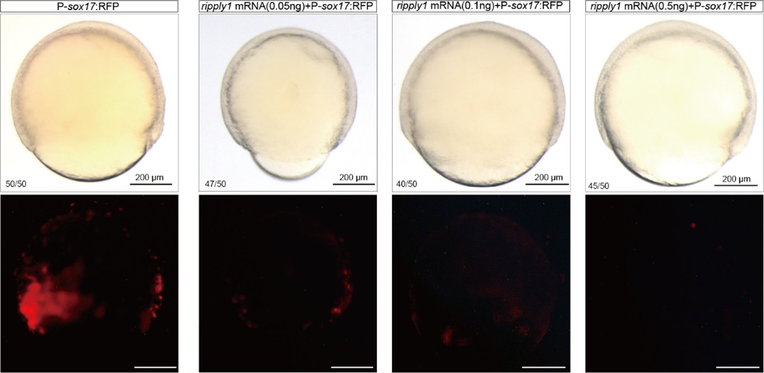
We sincerely thank the reviewer for raising this question. First, we apologize for not providing a detailed description of the amount of HA-ripply1 mRNA injected in our previous manuscript. We injected 500 pg of HA-ripply1 mRNA at the 1-cell stage and allowed the embryos to develop until 6 hpf for the CUT&Tag experiment. In the supplementary materials, we included a bright-field image of an 18 hpf-embryo injected with HA-ripply1 mRNA, which morphologically exhibited severe developmental abnormalities. The reviewer pointed out that the amount of ripply1 mRNA we injected might be excessive, potentially leading to non-specific gain-of-function effects. The injection dose of 500 pg was determined based on conclusions from our previous study. In that study, injecting 24 pg of ripply1 mRNA into one cell of zebrafish embryos at the 16–32 cell stage was sufficient to induce a secondary axis lacking the forebrain[5]. From this, we estimated that an injection concentration of approximately 500–1000 pg would be appropriate at the 1-cell stage, so that after several rounds of cell division, each cell gained 20-30 pg mRNA at 32 cell stage. Additionally, we conducted supplementary experiments injecting 100 pg, 250 pg, and 500 pg of ripply1 mRNA, and observed 500 pg of ripply1 mRNA led to a dramatic suppression of endoderm formation (Author response image 4).
Finally, our study focuses on the mechanism of cell fate segregation in the anterior mesendoderm, primarily during gastrulation. The embryos injected with ripply1 mRNA underwent normal gastrulation, and our CUT&Tag experiment was performed at 6 hpf. Therefore, we believe that the amount of ripply1 mRNA injected in this study is appropriate for addressing our research question.
Author response image 4.
Different concentrations of ripply1 mRNA were injected into zebrafish embryos at the one-cell stage, with RFP fluorescence labeling sox17-positive cells.
(4) Ripply1 binding to sox17 and sox32 regulatory regions not convincing: The Cut and Tag data presented in Fig 6J-K does not seem to be high quality and does not seem to provide strong support that Ripply 1 binds to the regulatory regions of these genes. The signal-to-noise ratio is very poor, and the 'binding' near sox17 that is identified seems to be even coverage over a 14 kb region, which is not consistent with site-specific recruitment of this factor, and the 'peaks' highlighted with yellow boxes do not appear to be peaks at all. To me, it seems this probably represents either: (1) overtagmentation of these samples or (2) an overexpression artifact from injection of too high concentration of ripply1-HA mRNA. In general, Cut and Tag is only recommended for histone modifications, and Cut and Run would be recommended for transcriptional regulators like these (see Epicypher's literature). Given this and the previous point about Ripply1 overexpression, I am not convinced that Ripply1 regulates endodermal genes. The existing data could be made somewhat more convincing by showing the tracks for other genes as positive and negative controls, given that Ripply1 has known muscle targets (how does its binding look at those targets in comparison) and there should be a number of Nodal target genes that Ripply1 does not bind to that could be used as negative controls. Overall this experiment doesn't seem to be of high enough quality to drive the conclusion that Ripply1 directly binds near sox17 and sox32 and from the data presented in the manuscript looks as if it failed technically.
We sincerely thank the reviewer for raising this question. We apologize that the binding regions of sox17 marked in our previous analysis were incorrect, and we have made the corresponding revisions in the latest version of the manuscript.
The reviewer noted that our CUT&Tag data contain considerable noise. To address this, we further refined our data processing: we annotated all peaks enriched in the treatment group and performed differential analysis, selecting genes with log<sub>2</sub>FoldChange > 3, padj < 0.5, and baseMean > 30 as candidate targets of Ripply1 binding. Subsequent GO enrichment analysis of these genes revealed significant enrichment of muscle development-related GO terms, which is consistent with previously reported roles of Ripply1 in regulating somite development. Therefore, we believe our filtering method effectively removes a large number of noise peaks and their associated genes.
Under these screening criteria, we found that sox32 meets the threshold, while sox17 does not. In addition, following the reviewer’s suggestion, we examined mespbb—a known gene repressed by Ripply1—and gsc, a Nodal target gene, as a negative control.
Based on these new analyses, we have revised our figures and text accordingly. Our data now support the possibility that Ripply1 may directly bind to the promoter region of sox32. Since sox32 acts as a direct upstream regulator of sox17, this binding could influence sox17 expression (Figure 6 and Figure S11).
Finally, we would like to note that studies have reported Ripply1 as a transcriptional repressor, which may function by recruiting other co-factors, such as Groucho, to form a complex[14,15]. This might explain why our CUT&Tag data detected Ripply1 binding to a broad set of genes.
(5) "Cooperatively Gsc and ripply1 regulate": I suggest avoiding the term "cooperative," when describing the relationship between Ripply1 and Gsc regulation of PP and anterior endoderm - it evokes the concept of cooperative gene regulation, which implies that these factors interact with each biochemically in order to bind to the DNA. This is not supported by the data in this manuscript, and is especially confusing since Ripply1 is thought to require cooperative binding with a T-box family transcription factor to direct its binding to the DNA.
We sincerely thank the reviewer for raising this important issue. The reviewer pointed out that the term "Cooperatively" may not be entirely appropriate in the context of our study. In accordance with the reviewer's suggestion, we have replaced "Cooperatively" with "Collectively" in the relevant sections.
(6) SWI/SNF: The differential expression of srcap doesn't seem very remarkable. The dot plots in the supplement S7H don't help - they seem to show no expression at all in the endoderm, which is clearly a distortion of the data, since from the violin plots it's obviously expressed and the dot-size scale only ranges from ~30-38%. Please add to the figure information about fold-change and p-value for the differential expression. Publicly available scRNAseq databases show scrap is expressed throughout the entire early embryo, suggesting that it would be surprising for it to have differential activity in these two cell types and thereby contribute to their separate specification during development. It seems equally possible that this just mildly influences the level of Nodal or FGF signaling, which would create this effect.
Thank the Reviewer for this question. As suggested, we performed Wilcoxon tests to compare srcap expression between PP and Endo populations. The analysis shows that while srcap expression is moderately elevated in PP compared to in Endo, this difference is not statistically significant. The corresponding p-value and fold change have now been included in the revised figure (Please see Figure 4J and S7H). Although the transcriptional level of srcap shows no significant difference between PP and anterior endoderm, our subsequent experiments—using AU15330 (an inhibitor of the SWI/SNF complex) and injecting morpholino targeting srcap, a key component of the SWI/SNF complex—demonstrated that its inhibition indeed promotes anterior endoderm fate while reducing PP cell specification. Therefore, we propose that subtle differences in the SWI/SNF complex may regulate the fate specification of PP and anterior endoderm through two mechanisms. First, as mentioned in our study, these chromatin remodelers modulate the expression of master regulators such as Gsc and Ripply1, thereby influencing cell fate decisions. Second, as noted by the reviewer, these chromatin remodelers may affect the interpretation of Nodal signaling, ultimately contributing to the divergence between PP and anterior endoderm fates.
The multiome data seems like a valuable data set for researchers interested in this stage of zebrafish development. However, the presentation of the data doesn't make many conclusions, aside from identifying an element adjacent to ripply1 whose chromatin is open in prechordal plate cells and not endodermal cells and showing that there are a number of loci with differential accessibility between these cell types. That seems fairly expected since both cell types have several differentially expressed transcriptional regulators (for instance, ripply1 has previously been demonstrated in multiple studies to be specific to the prechordal plate during blastula stages). The manuscript implies that SWI/SNF remodeling by Srcap is responsible for the chromatin accessibility differences between these cell types, but that has not actually been tested. It seems more likely that the differences in chromatin accessibility observed are a result of transcription factors binding downstream of Nodal signaling.
We thank the reviewer for recognizing the value of our newly generated data. Through integrative analysis of single-cell data from wild-type, ndr1 kd, and lft1 ko groups of Nodal-injected explants at 6 hours post-fertilization (hpf), we identified a critical branching point in the fate segregation of the prechordal plate (PP) and anterior endoderm (Endo), where chromatin remodelers may play a significant role. Based on this finding, we performed single-cell RNA and ATAC sequencing on zebrafish embryos at 6 hpf. Analysis of this multi-omics dataset revealed that transcriptional repressors such as Gsc, Ripply1, and Osr1 exhibit differences in both transcriptional and chromatin accessibility levels between the PP and anterior Endo. Subsequent overexpression and loss-of-function experiments further demonstrated that Gsc and Ripply1 collaboratively suppress endodermal gene expression, thereby inhibiting endodermal cell fate. Previous studies have reported that for the activation of certain Nodal downstream target genes, the pSMAD2 protein of the Nodal signaling pathway recruits chromatin remodelers to facilitate chromatin opening and promote further transcription of target genes[16]. Therefore, our data provide chromatin accessibility profiles for Gsc and Ripply1, offering a valuable resource for future investigations into their pSMAD2 binding sites.
Minor issues:
Figure 2 E-F: It's not clear which cells from E are quantitated in F. For instance, the dorsal forerunner cells are likely to behave very differently from other endodermal progenitors in this assay. It would be helpful to indicate which cells are analyzed in Fig F with an outline or other indicator of some kind. Or - if both DFCs and endodermal cells are included in F, to perhaps use different colors for their points to help indicate if their fluorescence changes differently.
Thank you for the reviewer's suggestion. In the revised version of the figure, we have outlined the regions of the analyzed cells.
Fig 3 J: Should the reference be Dubrulle et al 2015, rather than Julien et al?
Thanks, we have corrected.
References:
Alexander, J. & Stainier, D. Y. A molecular pathway leading to endoderm formation in zebrafish. Current biology : CB 9, 1147-1157 (1999).
Barone, V. et al. An Effective Feedback Loop between Cell-Cell Contact Duration and Morphogen Signaling Determines Cell Fate. Dev. Cell 43, 198-211.e12 (2017).
Economou, A. D., Guglielmi, L., East, P. & Hill, C. S. Nodal signaling establishes a competency window for stochastic cell fate switching. Dev. Cell 57, 2604-2622.e5 (2022).
Gritsman, K. et al. The EGF-CFC protein one-eyed pinhead is essential for nodal signaling. Cell 97, 121-132 (1999).
Gritsman, K., Talbot, W. S. & Schier, A. F. Nodal signaling patterns the organizer. Development (Cambridge, England) 127, 921-932 (2000).
Kawamura, A. et al. Groucho-associated transcriptional repressor ripply1 is required for proper transition from the presomitic mesoderm to somites. Developmental cell 9, 735-744 (2005).
Kawamura, A., Koshida, S. & Takada, S. Activator-to-repressor conversion of T-box transcription factors by the Ripply family of Groucho/TLE-associated mediators. Molecular and cellular biology 28, 3236-3244 (2008).
Sako, K. et al. Optogenetic Control of Nodal Signaling Reveals a Temporal Pattern of Nodal Signaling Regulating Cell Fate Specification during Gastrulation. Cell Rep. 16, 866-877 (2016).
Rogers, K. W. et al. Nodal patterning without Lefty inhibitory feedback is functional but fragile. eLife 6, e28785 (2017).
Warga, R. M. & Nüsslein-Volhard, C. Origin and development of the zebrafish endoderm. Development 126, 827-838 (1999).
References:
(1) Steinbeisser, H., and De Robertis, E.M. (1993). Xenopus goosecoid: a gene expressed in the prechordal plate that has dorsalizing activity. C R Acad Sci III 316, 959-971.
(2) Warga, R.M., and Nusslein-Volhard, C. (1999). Origin and development of the zebrafish endoderm. Development (Cambridge, England) 126, 827-838. 10.1242/dev.126.4.827.
(3) Sako, K., Pradhan, S.J., Barone, V., Inglés-Prieto, Á., Müller, P., Ruprecht, V., Čapek, D., Galande, S., Janovjak, H., and Heisenberg, C.P. (2016). Optogenetic Control of Nodal Signaling Reveals a Temporal Pattern of Nodal Signaling Regulating Cell Fate Specification during Gastrulation. Cell reports 16, 866-877. 10.1016/j.celrep.2016.06.036.
(4) van Boxtel, A.L., Economou, A.D., Heliot, C., and Hill, C.S. (2018). Long-Range Signaling Activation and Local Inhibition Separate the Mesoderm and Endoderm Lineages. Developmental cell 44, 179-191.e175. 10.1016/j.devcel.2017.11.021.
(5) Cheng, T., Xing, Y.Y., Liu, C., Li, Y.F., Huang, Y., Liu, X., Zhang, Y.J., Zhao, G.Q., Dong, Y., Fu, X.X., et al. (2023). Nodal coordinates the anterior-posterior patterning of germ layers and induces head formation in zebrafish explants. Cell reports 42, 112351. 10.1016/j.celrep.2023.112351.
(6) Economou, A.D., Guglielmi, L., East, P., and Hill, C.S. (2022). Nodal signaling establishes a competency window for stochastic cell fate switching. Developmental cell 57, 2604-2622 e2605. 10.1016/j.devcel.2022.11.008.
(7) Schier, A.F., and Talbot, W.S. (2005). Molecular genetics of axis formation in zebrafish. Annual review of genetics 39, 561-613. 10.1146/annurev.genet.37.110801.143752.
(8) Barone, V., Lang, M., Krens, S.F.G., Pradhan, S.J., Shamipour, S., Sako, K., Sikora, M., Guet, C.C., and Heisenberg, C.P. (2017). An Effective Feedback Loop between Cell-Cell Contact Duration and Morphogen Signaling Determines Cell Fate. Developmental cell 43, 198-211.e112. 10.1016/j.devcel.2017.09.014.
(9) Muller, P., Rogers, K.W., Jordan, B.M., Lee, J.S., Robson, D., Ramanathan, S., and Schier, A.F. (2012). Differential diffusivity of Nodal and Lefty underlies a reaction-diffusion patterning system. Science (New York, N.Y.) 336, 721-724. 10.1126/science.1221920.
(10) Rogers, K.W., Lord, N.D., Gagnon, J.A., Pauli, A., Zimmerman, S., Aksel, D.C., Reyon, D., Tsai, S.Q., Joung, J.K., and Schier, A.F. (2017). Nodal patterning without Lefty inhibitory feedback is functional but fragile. eLife 6. 10.7554/eLife.28785.
(11) Thisse, B., Wright, C.V., and Thisse, C. (2000). Activin- and Nodal-related factors control antero-posterior patterning of the zebrafish embryo. Nature 403, 425-428. 10.1038/35000200.
(12) Eroglu, B., Wang, G., Tu, N., Sun, X., and Mivechi, N.F. (2006). Critical role of Brg1 member of the SWI/SNF chromatin remodeling complex during neurogenesis and neural crest induction in zebrafish. Developmental dynamics : an official publication of the American Association of Anatomists 235, 2722-2735. 10.1002/dvdy.20911.
(13) Hensley, M.R., Emran, F., Bonilla, S., Zhang, L., Zhong, W., Grosu, P., Dowling, J.E., and Leung, Y.F. (2011). Cellular expression of Smarca4 (Brg1)-regulated genes in zebrafish retinas. BMC developmental biology 11, 45. 10.1186/1471-213X-11-45.
(14) Kawamura, A., Koshida, S., Hijikata, H., Ohbayashi, A., Kondoh, H., and Takada, S. (2005). Groucho-associated transcriptional repressor ripply1 is required for proper transition from the presomitic mesoderm to somites. Developmental cell 9, 735-744. 10.1016/j.devcel.2005.09.021.
(15) Kawamura, A., Koshida, S., and Takada, S. (2008). Activator-to-repressor conversion of T-box transcription factors by the Ripply family of Groucho/TLE-associated mediators. Mol Cell Biol 28, 3236-3244. 10.1128/MCB.01754-07.
(16) Ross, S., Cheung, E., Petrakis, T.G., Howell, M., Kraus, W.L., and Hill, C.S. (2006). Smads orchestrate specific histone modifications and chromatin remodeling to activate transcription. EMBO J 25, 4490-4502. 10.1038/sj.emboj.7601332.