eLife Assessment

This important study examines the role of TNF in modulating energy metabolism during parasite infection. The authors perform an elegant set of studies combining genetics, small molecule perturbation, and phenotypic experiments to highlight a role for glycolysis and glucose transport in control of parasitemia. This solid work integrates an interesting set of observations that will be of interest to the Plasmodium and pathogenesis communities with an expanded set of experiments.

Reviewer #2 (Public review):

[Editors' note: this version has been assessed by the Reviewing Editor without further input from the original reviewers.]

Summary:

The premise of the manuscript by Matteucci et al. is interesting and elaborates a mechanism via which TNFa regulates monocyte activation and metabolism to promote murine survival during Plasmodium infection. The authors show that TNF signaling (via an unknown mechanism) induces nitrite synthesis, which (via yet an unknown mechanism), and stabilizes the transcription factor HIF1a. Furthermore, that HIF1a (via an unknown mechanism) increases GLUT1 expression and increases glycolysis in monocytes. The authors demonstrate that this metabolic rewiring towards increased glycolysis in a subset of monocytes is necessary for monocyte activation including cytokine secretion, and parasite control.

Strengths:

The authors provide elegant in vivo experiments to characterize metabolic consequences of Plasmodium infection, and isolate cell populations whose metabolic state is regulated downstream of TNFa. Furthermore, the authors tie together several interesting observations to propose an interesting model.

Weaknesses:

The authors show that TNFa induces GLUT1 in monocytes, but do not show a direct role for GLUT1 or glucose uptake in monocytes in host resistance to infection.

Author response:

The following is the authors’ response to the previous reviews

We thank the reviewers for their careful evaluation and constructive comments throughout the two rounds of revision. We hope that the revisions have satisfactorily addressed all concerns and that the manuscript is now suitable for publication.

This novel contribution highlights the role of this pro-inflammatory factor in the pathogenesis of and resistance to Plasmodium chabaudi infection in mice. While aspects of this response have been previously described, this study is the first to link the TNF–iNOS–HIF-1α axis to the in vivo mediation of malaria disease through its involvement in glucose metabolism. Despite well-documented metabolic alterations during malaria, including hypoglycemia and hyperlactatemia, the mechanisms underlying these changes and their relationship to host immune responses remain poorly understood. Addressing this gap is essential for elucidating how metabolic adaptation shapes disease outcomes during Plasmodium infection.

In response to the reviewer’s comments, we have revised the Abstract, Introduction, and Discussion to clearly distinguish between:

Previously established mechanisms (TNF–iNOS–HIF-1α–glycolysis axis), and

The novel contribution of our study (its in vivo integration during Plasmodium infection and association with host resistance).

Public Reviews:

Reviewer #2 (Public review):

Summary:

The premise of the manuscript by Matteucci et al. is interesting and elaborates a mechanism via which TNFa regulates monocyte activation and metabolism to promote murine survival during Plasmodium infection. The authors show that TNF signaling (via an unknown mechanism) induces nitrite synthesis, which (via yet an unknown mechanism), and stabilizes the transcription factor HIF1a. Furthermore, that HIF1a (via an unknown mechanism) increases GLUT1 expression and increases glycolysis in monocytes. The authors demonstrate that this metabolic rewiring towards increased glycolysis in a subset of monocytes is necessary for monocyte activation including cytokine secretion, and parasite control.

Strengths:

The authors provide elegant in vivo experiments to characterize metabolic consequences of Plasmodium infection, and isolate cell populations whose metabolic state is regulated downstream of TNFa. Furthermore, the authors tie together several interesting observations to propose an interesting model regarding

Weaknesses:

The main conclusion of this work - that "Reprogramming of host energy metabolism mediated by the TNF-iNOS-HIF1a axis plays a key role in host resistance to Plasmodium infection" is unsubstantiated. The authors show that TNFa induces GLUT1 in monocytes, but never show a direct role for GLUT1 or glucose uptake in monocytes in host resistance to infection (nor the hypoglycemia phenotype they describe).

We thank the reviewer for this important comment and for highlighting the need to clarify the mechanistic link between TNF-driven metabolic rewiring and host resistance to Plasmodium infection. As noted in our first revision, our primary objective was to investigate how TNF integrates systemic and cellular metabolic responses during infection in vivo. We demonstrate that glucose uptake is significantly increased in spleen and liver during infection in a partially TNF-dependent manner, and that TNF promotes GLUT1 expression (main glucose transporter in immune cells) and glycolysis specifically in monocytic cells. Importantly, to directly address the role of TNF signaling in myeloid cells, we also observed the same phenotype (higher parasitemia, but absence of hypothermia and hypoglycemia) in mice with conditional deletion of TNF receptor 1 in lysozyme M–expressing cells (TNFR1^ΔLyz2) (Figure 4P–R), thereby validating in a cell-specific context the findings previously observed in mice with global TNFR1 deficiency. Together, these findings support a functional link between TNF signaling in monocytes, induction of GLUT1-dependent glucose metabolism, and the regulation of both systemic metabolic responses and host resistance during experimental malaria.

While we agree that we do not demonstrate a cell-intrinsic role for GLUT1 in monocytes, multiple lines of evidence in our study support the functional relevance of glycolytic metabolism downstream of the TNF–iNOS–HIF-1α axis.

(1) First, we show that Pc infection results in a marked increase in glucose uptake in the spleen and liver, but not in skeletal muscle or adipose tissues (Figure 2K), and that this effect is absent in TNFR-/- mice (Figure 2L), indicating a TNF-dependent and tissue-specific metabolic reprogramming. We have also clarified in the Discussion that this process appears to be insulin-independent and likely driven by pro-inflammatory signals.

(2) Second, we show that the TNF–iNOS–HIF-1α axis. induces GLUT1 expression in monocytic cells (Figures 4M, 5D, 6L). This supports a model in which these cells contribute to observed systemic metabolic changes.

(3) Third, we also observed a similar phenotype—characterized by higher parasitemia but absence of hypothermia and hypoglycaemia-in mice with conditional deletion of TNF receptor 1 in lysozyme M–expressing cells (TNFR1^ΔLyz2) (Figure 4P–R), thereby validating in a cell-specific context the findings previously observed in mice with global TNFR1 deficiency. These findings indicate that disruption of glycolysis phenocopies key aspects of the TNF-driven metabolic and immunological response to infection. 

(4) Finally, we demonstrate that glycolytic metabolism is functionally relevant for host resistance. Pharmacological inhibition of glycolysis in vivo using 2-DG led to increased parasitemia (Figure 6O), resembling the impaired parasite control observed in HIF-1α^ΔLyz2, TNFR-/-, and iNOS-/- mice. These findings indicate that disruption of glycolysis phenocopies key aspects of the TNF–iNOS–HIF-1α axis deficiency, supporting the conclusion that this pathway is required to sustain glycolytic metabolism and effective parasite control during infection.

About the hypoglycemia phenotype and resistance, our previous study (PMID: 29805094) demonstrates that TNF-driven inflammation regulates systemic glucose metabolism during Plasmodium chabaudi infection. We showed that infection-induced hypoglycemia correlates with TNF levels and is associated with changes in parasite development. Specifically, leukocytes primed with IFNγ display increased expression of glucose metabolism and inflammatory genes, and TNFα-induced hypoglycemia is linked to the accumulation of non-proliferative trophozoite forms, whereas parasite replication (schizogony) occurs during host feeding. These findings indicate that blood glucose availability, regulated by TNF, directly influences parasite growth dynamics and infection outcome. Although the cellular mechanisms were not addressed in that study, our current work builds on these findings by identifying the TNF-iNOS–HIF-1α axis as a driver of GLUT1-dependent glycolysis in monocytes, linking systemic metabolic changes to a cell-intrinsic mechanism that contributes to host resistance. 

We agree that directly establishing the cell-intrinsic contribution of GLUT1 would require dedicated genetic approaches (e.g., conditional deletion in monocytes), which are beyond the scope of the present study. 

Comments on revisions:

The demonstration that the established TNF-iNOS-HIF-1α-glycolysis axis operates in vivo during P. chabaudi infection is valuable and relevant. However, it constitutes contextual validation and must be carefully described as such. This distinction, i.e., "what has already been shown vs. what is new" is not consistently reflected in the framing of the manuscript raising overstatement concerns. This is particularly evident in the abstract and other conclusive statements, where mechanistic novelty is implied, even when the underlying pathways/mechanisms are already known. To improve the manuscript, all sentences that refer to already established findings should be accurately described as such.

For example, the abstract states: "Here, we show that TNF signaling hampers physical activity, food intake, and energy expenditure while enhancing glucose uptake by the liver and spleen as well as controlling parasitemia in P. chabaudi-infected mice." In this sentence, the effects of TNF signaling on physical activity, food intake, energy expenditure, glucose metabolism and control of parasitemia are unequivocally established and therefore do not, in themselves, constitute new findings. Feeding behavior, not cell-intrinsic metabolism, may drive glycemic differences.

We thank the reviewer for this comment and for highlighting the importance of distinguishing systemic metabolic effects from cell-intrinsic mechanisms. We have now revised the manuscript to more consistently distinguish between previously established mechanisms and our novel findings, particularly in the Abstract and other summary statements, to avoid any potential overstatement.

We also would like to emphasize that, in both the Introduction and Discussion, we explicitly acknowledge that key components of the TNF–iNOS–HIF-1α–glycolysis axis have been previously described. In the Introduction, we cite studies demonstrating that TNF can induce glucose uptake and metabolic reprogramming in immune cells (refs. 14–17), as well as the role of HIF-1α as a central regulator of glycolysis and inflammation in myeloid cells (refs. 21–28). Similarly, in the Discussion, we detail prior evidence that TNF induces iNOS-derived RNI (refs. 51–54), that RNI stabilizes HIF-1α (ref. 52), and that HIF-1α drives the expression of glycolytic genes including GLUT1 (refs. 55–57). We also cite studies showing that TNF contributes to parasite control and glucose metabolism in malaria (refs. 58–61).

Importantly, while these pathways have been described in other contexts, their integration and functional relevance in vivo during Plasmodium infection, particularly in the context of host systemic metabolism and monocytic cell function, have not been previously demonstrated. Our study addresses this gap by showing that this axis operates during P. chabaudi infection and links inflammatory signaling to both cellular metabolic reprogramming and organismal metabolic changes.

Specifically, we demonstrate that TNF signaling drives increased glucose uptake in spleen and liver in a tissue-specific manner, promotes GLUT1 expression and glycolysis in monocytic cells, and that disruption of this axis (genetically or pharmacologically via glycolysis inhibition) impairs parasite control. In addition, we provide evidence connecting these cellular processes to systemic metabolic alterations, including hypoglycemia.

The authors propose that TNF signaling leads to GLUT1 upregulation (in inflammatory monocytes, MO-DCs, and within the liver and spleen) during Plasmodium infection, and that this results in increased glucose uptake contributing to systemic hypoglycemia. While this is an intriguing hypothesis, we urge the authors to consider an alternative explanation that, at present, is not adequately ruled out. Given that glycemia serves as a central functional readout in the manuscript, this distinction is essential to clarify.

The observed regulation of glycemia is likely not a direct consequence of increased glucose uptake by immune cells or by tissues but may instead reflect broader differences in disease severity across genotypes. The iNOS KO, TNFR KO, and HIF-1ΔLyz2 mice likely experience a dampened inflammatory response, which would blunt infection-induced anorexia and help preserve overall metabolic homeostasis. This alternate interpretation is supported by the authors' metabolic cage data showing increased physical activity in TNFR KO mice and the elevated food intake shown in Figure 2B.

We thank the reviewer for this important point regarding the potential contribution of feeding behavior and systemic energy balance to the observed metabolic phenotypes. In fact, this possibility has been explicitly already incorporated into the revised manuscript. Also, we have revised the Discussion to explicitly state that the hypoglycemia observed during infection likely reflects both systemic changes in energy balance and TNF-driven metabolic reprogramming in immune cells, rather than a single isolated mechanism. Specifically, we have had already added the following statement to the Discussion:

“Although restored physical activity, food consumption and energy expenditure in knockout mice may contribute to the observed systemic metabolic parameters by altering energy balance, these effects are not mutually exclusive with the TNF-driven, cell-intrinsic metabolic mechanisms described here”.

In addition, we note that under naive conditions, we did not observe differences between genotypes in physical activity, food intake, energy expenditure, respiratory exchange ratio, or glycemia. These findings support that baseline metabolic parameters are comparable and that the differences observed during infection arise in the context of TNF-dependent inflammatory responses. During infection, although TNFR-deficient mice display increased food intake and activity, these differences arise in the context of altered inflammatory signaling. Therefore, rather than being mutually exclusive, behavioral and metabolic changes are likely coordinated downstream of TNF signaling.

Furthermore, our data using pharmacological inhibition of glycolysis (2-deoxy-D-glucose) demonstrate that disruption of glycolytic metabolism results in increased parasitemia and reduced lactate levels, recapitulating key aspects of the phenotype observed in TNFR-/-, iNOS-/-, and HIF-1αΔLyz2 mice. This supports a functional role for glycolytic metabolism in host response, beyond differences in feeding behavior.

Since anorexia and energy expenditure are tightly coupled to the inflammatory milieu, it is plausible that these behavioral and systemic differences-not monocyte nor tissue GLUT1 expression per se-are the primary contributors to the observed glycemic patterns. To support their current interpretation, the authors should perform a pair-feeding experiment in which (at least) TNFR KO mice are restricted to the same food intake as infected WT controls. This would help disentangle whether differences in glycemia truly reflect immune-driven metabolic rewiring or are secondary to differences in caloric intake.

We thank the reviewer for this suggestion. We agree that pair-feeding experiments would provide an additional layer of control to isolate the contribution of caloric intake. However, we note that:

(1) Baseline metabolic equivalence in naive animals argues against intrinsic differences in energy balance.

(2) The observed phenotypes occur in the context of infection-driven inflammation, where anorexia is itself a TNF-dependent host response.

(3) Our data support a model in which behavioral changes and metabolic rewiring are integrated components of the host response rather than independent variables.

Importantly, our data already support a role for TNF-driven metabolic rewiring beyond feeding behavior, as inhibition of glycolysis with 2-deoxy-D-glucose recapitulates the impaired parasite control observed in genetic models. In addition, as discussed in the manuscript, systemic factors such as food intake are not mutually exclusive with cell-intrinsic metabolic mechanisms.

We therefore consider that pair-feeding experiments are beyond the scope of the present study.

The contribution of monocyte-specific glucose metabolism to host resistance remains unresolved.

We appreciate the authors' effort to address the mechanistic role of glycolysis in host resistance using in vivo 2-deoxyglucose (2DG) treatment. However, I would like to point out that while this experiment is informative, it does not fully resolve the specific concern raised regarding the cell-intrinsic role of TNF-induced glycolysis in monocytes. 2DG acts systemically, inhibiting glycolysis across a wide range of cell types-including hepatocytes, endothelial cells, lymphocytes, and myeloid populations. Therefore, the observed increase in parasitemia following 2DG treatment may reflect the broad importance of glycolysis for host defense, or alternatively, may result from elevated circulating glucose levels induced by 2DG (PMID: 35841892), which could enhance parasite growth by increasing nutrient availability. Therefore, this experiment does not allow for a specific conclusion about the requirement for TNF-driven metabolic reprogramming in monocytes.

We thank the reviewer for this comment regarding the interpretation of the 2-deoxyglucose (2DG) experiments. We agree that systemic 2DG treatment does not allow cell-specific conclusions, as it broadly inhibits glycolysis across multiple cell types. Accordingly, these data are interpreted as supporting a role for glycolysis in host defense at the organismal level, rather than as direct evidence for a monocyte-intrinsic requirement of TNF-driven metabolic reprogramming.

At the same time, our study includes cell-specific analyses that support the engagement of this pathway in myeloid populations. In particular, we observe increased GLUT1 expression in CD11b⁺ cells within both the liver and spleen during infection, with marked upregulation in monocyte-derived dendritic cells (MODCs). Importantly, this induction is not observed in the corresponding knockout models, supporting the idea that TNF signaling is required for this metabolic adaptation in these cells in vivo. Consistent with this, we validated that both parasitemia and systemic glucose levels in TNFR1^ΔLyz2 mice phenocopy those observed in TNFR-deficient animals, reinforcing the contribution of myeloid TNF signaling to the metabolic and disease outcomes.

In addition, our in vitro data demonstrate increased GLUT1 expression in WT monocytes but not in cells lacking components of the TNF–iNOS–HIF-1α axis, further supporting a pathway-specific effect. Given that GLUT1 is the primary glucose transporter in immune cells, these combined in vivo and in vitro findings, together with the 2DG experiments, provide strong evidence supporting our proposed model. 

We agree that directly establishing a monocyte-intrinsic role would require targeted genetic approaches, which are beyond the scope of the present study.

eLife Assessment

This valuable study characterizes the emergence of the membrane-associated periodic cytoskeleton (MPS) in the axons of human motor neurons derived from induced pluripotent stem cells. Super-resolution imaging of beta-II spectrin provides convincing evidence for the patterned assembly of spectrin-poor gaps and spectrin-rich MPS in the medial region of the axons and its enhancement by the kinase inhibitor staurosporine. The data advocates against gap formation by axonal degeneration or cytoskeleton disassembly in a continuous MPS. Instead, a continuous MPS may result from nascent MPS patches and their maturation, a model that would benefit from live imaging for validation.

Reviewer #1 (Public review):

The authors have presented a revised version of their investigation into the Membrane Associated Periodic Skeleton (MPS) in iPSC derived human motor neurons. As mentioned in the earlier report, the main observations reported in this article-occurrence of patch and gap arrangement of MPS-is very interesting. The real puzzle is whether, and if so how, this structure coarsens over time to produce continuous MPS.

Following suggestions from reviewers, the authors attempted live cell imaging, but the results were not consistent enough and the authors point out difficulties in obtaining sufficient numbers and possible artefacts of over-expression. This investigation would have been much stronger with live cell imaging data on the dynamics of patch and gap structures.

Reviewer #2 (Public review):

Summary:

In this manuscript, Gazal et al., describe the presence of unique gaps and patches of BetaII-spectrin in medial sections of long human motor neuron axons. BII-spectrin, along with Alpha-spectrin forms horizontal linkers between 180nm spaced F-actin rings in axons. These F-actin rings along with the spectrin linkers form membrane periodic structures (MPS) which are critical for maintenance of the integrity, size and function of axons. The primary goal of the authors was to address if long motor axons, particularly those carrying familial mutations associated with the neurodegenerative disorder ALS, show defects in gaps and patches of BetaII-spectrin ultimately leading to degradation of these neurons.

Strengths:

The experiments are well designed and the authors have used the right methods and cutting-edge techniques to address the questions in this manuscript. The use of human motor neurons and the use of motor neurons with different familial ALS mutations is a strength. The use of isogenic controls is a positive. The induction of gaps and patches by the kinase inhibitor staurosporine and their rescue by Latrunculin A is novel and well executed. The use of biochemical assays to explore the role of calpains is appropriate and well designed. The use of STED imaging to define the periodicity of MPS in the gaps and patches of spectrin is a strength.

Weaknesses:

Primary weakness is the lack of rigorous evaluation to validate the proposed model of spectrin capture from the gaps into adjacent patches by the use of photobleaching and live-imaging. Another point is the lack of investigation into how gaps and patches change in axons carrying the familial ALS mutations as they age, since 2 weeks is not a timepoint when neurodegeneration is expected to start.

Comment on revised version.

The authors have given a point-by-point response to all the reviewer's concerns. They have also addressed concerns which I raised adequately. I have no further concerns.

Reviewer #3 (Public review):

Summary:

Gazal et al present convincing evidence supporting a new model of MPS formation where a gap-and-patch MPS pattern coalesces laterally to give rise to a lattice covering the entire axon shaft.

Strengths:

(1) This is a very interesting study that supports a change in paradigm in the model of MPS lattice formation.

(2) Knowledge on MPS organization is mainly derived from studies using rat hippocampal neurons. In the current manuscript, Gazal et al use human IPS-derived motor neurons, a highly relevant neuron type to further the current knowledge on MPS biology.

(3) The quality of the images provided, specifically of those involving super-resolution is of high standards, supporting adequately the conclusions of the authors.

Weaknesses:

(1) The main concern raised by the manuscript is the assumption that staudosporine-induced gap and patch formation recapitulates the physiological assembly of gaps and patches of betaII-spectrin.

(2) One technical challenge that limits a more compelling support of the new model of MPS formation, is that fixed neurons are imaged, which precludes the observation of patch coalescence.

Author response:

The following is the authors’ response to the original reviews.

eLife Statement

This valuable study characterizes the emergence of the membrane-associated periodic cytoskeleton (MPS) in the axons of human motor neurons derived from induced pluripotent stem cells. Super-resolution imaging of beta-II spectrin provides convincing evidence for the patterned assembly of spectrin-poor gaps and spectrin-rich MPS in the medial region of the axons and its enhancement by the kinase inhibitor staurosporine. The data advocates against gap formation by cytoskeleton disassembly in a continuous MPS. Instead, a continuous MPS may result from nascent MPS patches and their maturation, a model that would benefit from live imaging for validation.

(R1) We thank the reviewers and editor for their constructive and thoughtful feedback. We are pleased the reviewers found our evidence to be convincing and that our study provides a valuable framework for understanding the complex dynamics of MPS assembly.

Public Reviews:

Reviewer #1 (Public review):

Summary:

Ever since the surprising discovery of the membrane-associated Periodic Skeleton (MPS) in axons, a significant body of published work has been aimed at trying to understand its assembly mechanism and function. Despite this, we still lack a mechanistic understanding of how this amazing structure is assembled in neuronal cells. In this article, the authors report a "gap-and-patch" pattern of labelled spectrin in iPSC-derived human motor neurons grown in culture. The mid-sections of these axons exhibit patches with reasonably well-organized MPS that are separated by gaps lacking any detectable MPS and having low spectrin content. Further, they report that the intensity modulation of spectrin is correlated with intensity modulations of tubulin as well. However, neurofilament fluorescence does not show any correlation. Using DIC imaging, the authors show that often the axonal diameter remains uniform across segments, showing a patch-gap pattern. Gaps are seen more abundantly in the midsection of the axon, with the proximal section showing continuous MPS and the distal segment showing continuous spectrin fluorescence but no organized MPS. The authors show that spectrin degradation by caspase/calpain is not responsible for gap formation, and the patches are nascent MPS domains. The gap and patch pattern increases with days in culture and can be enhanced by treating the cells using the general kinase inhibitor staurosporine. Treatment with the actin depolymerizing agent Latrunculin A reduces gap formation. The reasons for the last two observations are not well understood/explained.

(R2) We thank the reviewer for the detailed and accurate description of the data shown and its relevance to further our understanding of MPS assembly mechanism and function.

Strengths:

The claims made in the paper are supported by extensive imaging work and quantification of MPS. Overall, the paper is well written and the findings are interesting. Although much of the reported data are from axons treated with staurosporine, this may be a convenient system to investigate the dynamics of MPS assembly, which is still an open question.

(R3) We thank the reviewer for the positive comments on the manuscript and the convenience of the experimental system developed to further study the dynamics of MPS assembly. We hope others turn into motor neurons to explore cortical cytoskeleton biology and hopefully shed light into their susceptibility in various degenerative diseases.

Weaknesses:

Much of the analysis is on staurosporine-treated cells, and the effects of this treatment can be broad. The increase in patch-gap pattern with days in culture is intriguing, and the reason for this needs to be checked carefully. It would have been nice to have live cell data on the evolution of the patch and gap pattern using a GFP tag on spectrin. The evolution of individual patches and possible coalescence of patches can be observed even with confocal microscopy if live cell super-resolution observation is difficult.

(R4) Because staurosporine may hit various kinases relevant to the phenomenon under study we did not elaborate too deeply on the likely targets in the discussion. We have, however, included the possibility that the relevant kinase in this matter could be PKC, in light of the new study published while our manuscript was under revision (Heller et al., 2025) (see second last paragraph in the Discussion section). Staurosporine represented a convenient initial approach that allowed us to find the phenomenon, and we are now conducting new studies dissecting the molecular pathways involved. However, the extent of such studies lies beyond the scope of the present report.

See R16 regarding possible live-imaging experiments using tagged βII-spectrin constructs.

Some more comments:

(1) Axons can undergo transient beading or regularly spaced varicosity formation during media change if changes in osmolarity or chemical composition occur. Such shape modulations can induce cytoskeletal modulations as well (the authors report modulations in microtubule fluorescence). The authors mention axonal enlargements in some instances. Although they present DIC images to argue that the axons showing gaps are often tubular, possible beading artefacts need to be checked. Beading can be transient and can be checked by doing media changes while observing the axons on a microscope.

(R5) As we acknowledge this possibility, we believe that, even if they occurred, they could not contribute to our observations of gaps-and-patches phenomenon since this latter subsisted long (hours and days) after any gross manipulation of media. Moreover fixed samples, when observed under DIC, confocal or STED did not evidence such beadings. We do refer to a characteristic local enlargement that was very localized and very low in numbers (see Fig.1C and E, and Suppl. Fig1C and E), so we don't believe these are transient, and do not resemble the structure referred to as beading. Structurally, beading is essentially different since it appears in rows of consecutive “beads” in long stretches, where round, small enlargements of axonal caliber are arranged in a consecutive manner, resembling pearls on a string. As mentioned by the reviewer, the beading phenomena can occur transiently when drastically changing media osmolarity (rarely done in cell culture manipulations) or non-tranciently when axons are undergoing degeneration. Indeed, to prevent gross changes in osmolarity, our routine fixation is a 4% PFA and 4% sucrose in PBS. In any case, we did not observe signs of beading in the cultures used for this study.

(2) Why do microtubules appear patchy? One would imagine the microtubule lengths to be greater than the patch size and hence to be more uniform.

(R6) Our stainings are for tubulin protein isoforms beta-III and alpha-II. That is, they would label microtubules, but free tubulin as well. Hence we don't think this is evidence for “patchy microtubules”. The slight decrease in intensity for tubulin within gaps is indeed something to investigate, and can indicate that tubulin prefers to accumulate within patches.

(3) Why do axons with gaps increase with days in culture? If patches are nascent MPS that progressively grow, one would have expected fewer gaps with increasing days in culture. Is this indicative of some sort of degeneration of axons?

(R7) We agree with the apparent discrepancy. However, one has to take into account that these axons are still elongating even at 2 weeks in culture and beyond. Hence, at any time point, there is a new axonal compartment recently added, and hence, with low βII-spectrin and no organized MPS. Also, the dynamical evolution of the gaps-and-patches structure has to take into account the rate of βII-spectrin supply and transport. If supply is somehow lower than a given threshold, it is expected that there will be more gaps, given the new, more distant parts of the axons have a lower supply of βII-spectrin. To explore this formally, we are working on simulations of these multifactorial dynamic systems to better understand this, that together with key experimental observations would enhance our understanding into our model of MPS assembly in growing axons. However, findings for this project will be the subject of another manuscript.

(4) It is surprising that Latrunculin A reduces gap formation induced by staurosporine (also seems to increase MPS correlation) while it decreases actin filament content. How can this be understood? If the idea is to block actin dynamics, have the authors tried using Jasplakinolide to stabilize the filaments?

(R8) The results with the co-treatment with Latrunculin A and Staurosporine are indeed intriguing, and provide clear evidence that the gap-and-patch pattern arises from local assembly of the MPS, requiring newly formed actin filaments. On the other hand, the fact that F-actin within the pre-formed MPS seems unaffected is not surprising. There are many different populations of F-actin in axons (i.e. MPS rings, longitudinal filaments, actin patches, actin trails), all of which have a different rate of monomer turnover. Latrunculin A affects filaments indirectly. The target of Latrunculin A is not actin filaments, but free monomers. Monomer sequestration ultimately affects actin filaments: filaments are constantly exchanging monomers, but, devoid of free monomers, filaments get shorter and eventually disappear. The drastic decrease in global F-actin in LatA-treated axons reflects that. The fact that F-actin in the MPS is preserved shows that these filaments are stable -if they are not losing monomers in the time frame of the treatment, the filament remains unaffected. This subject is extensively covered in the 8th paragraph of the Discussion section.

We have not used Jasplakinolide. The expected outcome will not mimic that of Latrunculin A since Jasplakinolide has a different mechanism of action (i.e. it binds -and stabilizes- the actin filament).

(5) The authors speculate that the patches are formed by the condensation of free spectrins, which then leaves the immediate neighborhood depleted of these proteins. This is an interesting hypothesis, and exploring this in live cells using spectrin-GFP constructs will greatly strengthen the article. Will the patch-gap regions evolve into continuous MPS? If so, do these patches expand with time as new spectrin and actin are recruited and merge with neighboring patches, or can the entire patch "diffuse" and coalesce with neighboring patches, thus expanding the MPS region?

(R9) We agree with the reviewer's interpretation. A virtue of our experimental model and our interpretations of the observations in fixed cells is that it gives rise to informative questions such as the ones posed by the reviewer. See R16 regarding possible live-imaging experiments using tagged βII-spectrin constructs.

Reviewer #2 (Public review):

Summary:

In this manuscript, Gazal et al. describe the presence of unique gaps and patches of BetaII-spectrin in medial sections of long human motor neuron axons. BII-spectrin, along with Alpha-spectrin, forms horizontal linkers between 180nm spaced F-actin rings in axons. These F-actin rings, along with the spectrin linkers, form membrane periodic structures (MPS) which are critical for the maintenance of the integrity, size, and function of axons. The primary goal of the authors was to address whether long motor axons, particularly those carrying familial mutations associated with the neurodegenerative disorder ALS, show defects in gaps and patches of BetaII-spectrin, ultimately leading to degradation of these neurons.

(R10) We thank the reviewer for the detailed and accurate description of the data shown.

Strengths:

The experiments are well-designed, and the authors have used the right methods and cutting-edge techniques to address the questions in this manuscript. The use of human motor neurons and the use of motor neurons with different familial ALS mutations is a strength. The use of isogenic controls is a positive. The induction of gaps and patches by the kinase inhibitor staurosporine and their rescue by Latrunculin A is novel and well-executed. The use of biochemical assays to explore the role of calpains is appropriate and well-designed. The use of STED imaging to define the periodicity of MPS in the gaps and patches of spectrin is a strength.

(R11) We thank the reviewer for the positive comments on the manuscript, the techniques used and the proposed model.

Weaknesses:

The primary weakness is the lack of rigorous evaluation to validate the proposed model of spectrin capture from the gaps into adjacent patches by the use of photobleaching and live imaging. Another point is the lack of investigation into how gaps and patches change in axons carrying the familial ALS mutations as they age, since 2 weeks is not a time point when neurodegeneration is expected to start.

(R12) See R16 regarding possible live-imaging experiments using tagged βII-spectrin constructs.

We don't discard the notion that axons carrying familial ALS mutations will show defects in MPS formation and/or stability when observed at longer culture times, or under culture conditions that promote neuronal aging (Guix et al., 2021). Thus, we continue to work with these cells, but the goal of such project lies well beyond the primary message of the present manuscript, as we discuss in the second paragraph of the Discussion section.

Reviewer #3 (Public review):

Summary:

Gazal et al present convincing evidence supporting a new model of MPS formation where a gap-and-patch MPS pattern coalesces laterally to give rise to a lattice covering the entire axon shaft.

Strengths:

(1) This is a very interesting study that supports a change in paradigm in the model of MPS lattice formation.

(2) Knowledge on MPS organization is mainly derived from studies using rat hippocampal neurons. In the current manuscript, Gazal et al use human IPS-derived motor neurons, a highly relevant neuron type, to further the current knowledge on MPS biology.

(3) The quality of the images provided, specifically of those involving super-resolution, is of a high standard. This adequately supports the conclusions of the authors.

(R13) We thank the reviewer for the positive comments on the manuscript, the techniques used and the proposed model.

Weaknesses:

(1) The main concern raised by the manuscript is the assumption that staudosporine-induced gap and patch formation recapitulates the physiological assembly of gaps and patches of betaII-spectrin.

(R14) Along the project, various gaps-and-patches parameters were measured in different conditions and stainings. In all these examinations the only parameter that changed considerably was their abundance. While this suggests that the gaps-and-patches features are comparable between control and staurosporine-treated cells, we acknowledge as a general caution regarding negative data—that subtle qualitative differences cannot be entirely ruled out. We have now emphasized this possibility in the 9th paragraph of the Discussion section.

(2) One technical challenge that limits a more compelling support of the new model of MPS formation is that fixed neurons are imaged, which precludes the observation of patch coalescence.

(R15) See R16 regarding possible live-imaging experiments using tagged βII-spectrin constructs.

Recommendations for the authors:

Reviewing Editor Comments:

The reviewers all agree that the work would strongly benefit from live imaging to assess the maturation dynamics of the gap/patch pattern.

(R16) Reviewers agreed that some of the conclusions of our manuscript would benefit from live imaging for validation. Various anticipated technical and biological challenges made these approaches not to be conducted for this initial study on human motor neurons. Just to mention the most important, from previous work of our labs, these cells themselves are difficult to transfect at 2 weeks in culture. Also, ectopically expression of tagged βII-spectrin escapes normal expression control and it has been noticed that ectopic expression yields to protein localization that does not necessarily reflect the endogenous distribution, or that produces cellular responses that precludes the observation of the phenomena under study. These difficulties in studying over-expressed tagged βII-spectrin have been reported in the field, with mentions that the analysed axons were those expressing “low levels of the construct” (Boyer et al., 2026; Zhong et al., 2014; Zhou et al., 2022). Taking this into account, we did not anticipate that, for the goals of the present project, live-imaging was to be included. However, given the positive comments and reception of our conclusions, we sought to try to perform this challenging and risky approach. To that end, we used a C-terminus tagged mouse βII-spectrin-GreenLantern plasmid to transfect our cells (a kind gift from Dr. Subjohit Roy, UCSD, USA). After 3 rounds of differentiating cells and trying various combinations of plasmid quantity, lipofectimine-to-DNA ratios and times of transfection (amongst other parameters), we have got an extremely low efficiency of transfection, and the few expressing neurons showed a distribution of βII-spectrin-GreenLantern that did not match our observations of immunolocalization of endogenous βII-spectrin. Taking all these into account, the present version of the manuscript will not include live-cell imaging on expressed tagged βII-spectrin. Given that reviewers found that some statements in the initial submission would have been better supported by live-imaging, we made changes in the manuscript so as to acknowledge the limitations of concluding dynamic mechanisms from fixed samples (see for example last sentences on 5th paragraph of the Discussion section). Having said so, we hope to be able, in the future, to overcome these experimental challenges and be able to establish live-imaging of βII-spectrin in neurons. For example, to avoid unregulated transgene expression, Heller and colleagues recently generated a βII- spectrin-mNeonGreen conditional knock-in (cKI) mice, consisting of a LoxP- flanked alternative final exon of endogenous βII-spectrin with a C- terminal mNeonGreen fusion that is expressed upon Cre expression (Heller et al., 2025). The implementation and further development of such approaches will be very helpful in new studies on the dynamics of βII-spectrin and the MPS as a whole. However, the scale of work needed to accomplish those approaches represent stand-alone projects.

Reviewer #1 (Recommendations for the authors):

In the section "The MPS is absent in beta-II spectrin gaps, the authors mention that the presence of MPS in patches suggests that the axons are not undergoing degeneration. I don't think this is a good criterion to use, despite the citations they take support from.

(R17) We agree with the reviewer's suggestion: in virtue of the unlikely connection between the cited developmental axon degeneration process in sensory neurons and the possible axon degeneration of long term cultures of human-iPSCs-derived motor neurons studied here, we have eliminated the sentence of reference

The authors show that degradation by proteases does not happen in their case. In this regard, they may want to discuss the recent article by Heller et al, Science 2025 (https://doi.org/10.1126/science.adn6712) and Hofmann et al, Sci. Rep., 2022 (https://doi.org/10.1038/s41598-022-18562-5)

(R18) By western blot analysis, we did not see evident changes in proteolysis-derived fragments. However it is likely that even when finding phenotypes with protease inhibitors, protein fragments accumulation is below the sensitivity of western blots. We were expecting gross changes observable by western blot in the case proteolysis explained gap formation.

Calpain and Caspase activity has been shown to be relevant in different aspects of MPS biology. To the works cited by the reviewer, now one has to add the very recent work by Fei and colleagues (Fei et al., 2026). We have modified part of the Discussion section to analyse our results in this broader context.

Briefly, Hofmann and colleagues found that acute treatment with calpain inhibitors right before axotomy lead to an increase in percentage of periodic βII-spectrin (referred by authors as “periodicity”) in the regenerated axons in a 2-hour period. Interestingly, the βII-spectrin patches they describe at distal portions did not increase in number, but they increased in size. This indicates that in the particular situation of axonal regeneration calpain activity puts a brake into MPS formation within patches. This invited us to re-examine our own protease inhibition experiments, and measured patch length in this. The new results are shown in Supplementary Fig. 6 and and further analysed in the Discussion section. In summary, our changes were much less notable than the ones found in regenerating axons, but follow the same trend: protease inhibitors made patches longer.

On the other hand, Heller and colleagues found in live-imaging studies that calpain activity contributes to the steady-state dynamics of βII-spectrin exchange in a mature MPS lattice. More recently, Fei and colleagues found that caspase or calpain inhibition does not change the steady-state organization of a mature MPS lattice when observing treated axons after fixation samples. Fei and colleagues find a relevant role for calpains whenever massive endocytosis (of any kind) is engaged experimentally. Interestingly, all these studies, including ours, examined calpains roles in MPS in different scenarios. When looked in detail, we don’t believe that these are contradictory results among them, and a complete picture of calpains (and caspases) roles in MPS assembly, growth, maintenance and remodeling will have to take into account all the above mentioned results, including ours. All these analyses are now included in the Discussion section.

Minor comments:

(1) "Recently, it was proposed that this continuous MPS organization arises from the coalescence of discontinuous "patches" of incomplete MPS units that originate in the distal axon and migrate proximally (Zhong et al. 2014)." Please check the citation. Should it be Hoffman et al. 2022?

(R19) The reviewer is correct. The proper citation has now been included.

(2) Is there an established link between ALS and spectrin? I would suggest decreasing the emphasis on this as no clear conclusions are achieved.

(R20) As stated in the text, the study of ALS mutations is justified from two aspects: one aspect is that there are several tubulin and other cytoskeletal proteins whose mutations are linked to ALS (Castellanos-Montiel et al., 2020) and microtubules dynamics has been shown to affect the cortical skeleton (Qu et al., 2017). Second, since human motor neurons are affected in ALS, we thought that a complete characterization of the βII-spectrin cortical cytoskeleton in these cells should include ALS-related mutations. We have now included an a basic MPS description in TDP43 and SOD1 mutation (Suppl. Fig. 5).

The aspect of ALS-related mutations only occupies two short paragraphs in the main text and some panels in Supplementary information. To follow the suggestions by the Reviewer, we have downplayed the relative relevance of these results in the text, without compromising the amount of data we show.

(3) There is a typo in the approximate symbol used for 150 kDa in the section where calpain and caspase activity is reported.

(R21) Typo corrected.

(4) Please add the Latrunculin concentration used in the main text, as it makes it easier for the reader.

(R22) Done.

(5) In the Discussion, paragraph starting with "We further showed ...", there is a typo where Zhong et al is cited.

(R23) Corrected.

(6) Supplementary Figure 1B: attachment instead of 'atachment'.

(R24) Corrected.

(7) Include DIVs or time in the schematic. It is easier for the reader to understand.

(R25) We have now included time references in schematics of Suppl. Fig1B.

(8) Supplementary Figure 1C

Unable to distinguish βII-spectrin and βIII-tubulin in the merged image. Separate figure panels will help.

(R26) The merged images in the reconstructions are merely to better show the tracing individual axons at such low magnification. Relevant portions with only βII-spectrin channels are shown in C1 and C2. Separated individual channels are shown elsewhere across the manuscript.

(9) Supplementary Figure 4D

Why is there so much cleavage product for αII-spectrin across DMSO and treatment? It varied over batches as well. Doesn't this mean that αII-spectrin is going through more proteolytic cleavage? Why?

(R27) The amount of cleavage product for αII-spectrin is not a surprise to us. For instance, although calpains and caspases can potentially process both α- and β-spectrin, in in vivo scenarios where calpain activity is triggered there are much more fragments of α-spectrin being produced (Czogalla & Sikorski, 2005). On the other hand, our staining of cleaved-αII-spectrin by the SNTF antibody by immunofluorescence (Fig4C) parallels the findings by western blot -high levels of cleaved-αII-spectrin across treatments. A similar strong staining using this antibody has been recently shown in the intact axon (Heller et al., 2025). It will be interesting in the future to address if these fragments have any biological significance beyond being mere byproducts of αII-spectrin processing.

Reviewer #2 (Recommendations for the authors):

Suggestions for improving the quality of the manuscript:

(1) Live imaging in combination with FRAP assays will help define whether the capture of spectrin from gaps into patches is true. Fixed neurons only provide static information and may not reflect real-time physiological effects.

(R28) See R16 regarding possible live-imaging experiments using tagged βII-spectrin constructs.

(2) Could the presence of F-actin trails in axons facilitate the formation of patches? Will the use of formin/Arp2/3 inhibitors rescue the effect of staurosporine, similar to Latrunculin A?

(R29) Very interesting suggestion. It is likely that different pools of F-actin contribute to the dynamic of MPS formation, and actin trails are definitely worth investigating in this context.

(3) Figure 8 lacks a latrunculin A treated condition? Why is this not present?

(R30) The quantification of that treatment was excluded for space and readability. We have now included the values of group LatA + DMSO in Fig8Cand D and rearranged the whole figure.

(4) Does neuronal stimulation have any effect (KCl treatment) on gaps and patches?

(R31) Very interesting suggestion. Unfortunately, we have not examined whereas neuronal stimulation affects any parameter of the gaps-and-patches structure.

(5) Please check the manuscript for typos and reference insertion points in the text. More than a couple were noted.

(R32) We have corrected typos.

Reviewer #3 (Recommendations for the authors):

This is a very interesting study that supports a change in paradigm in the model of MPS lattice formation.

(1) One major concern is the assumption that staudosporine-induced gap and patch formation recapitulates the physiological assembly of gaps and patches of betaII-spectrin, solely based on their morphological similarity. This should be further discussed in the manuscript. Further analysis of additional cytoskeleton components, including microtubules in staurosporine-treated neurons, could also be provided.

(R33) See R14.

(2) In Figure 1E, betaIII-tubulin and NF-H seem to accumulate in betaII-spectrin-rich axonal enlargements. If these are patches, how do you reconcile this finding with Figure 2C-D, where NF-M and alphaII-tubulin are not specifically enriched in betaII-spectrin patches?

(R34) We actually show that axonal enlargements and patches are structurally unrelated, in many aspects. We mention these axonal enlargements as a way to perform an exhaustive characterization of all βII-spectrin features found in these axons.

(3) One technical challenge that limits a more compelling support of the new model of MPS formation is that fixed neurons are imaged, which precludes the observation of patch coalescence. This should be further discussed in the revised version of the manuscript.

(R35) The limitation of the experimental approach is now further discussed (see for example last sentences on 5th paragraph of the Discussion section).

(4) On a more general note, the title of some of the Results sub-sections could be revised to convey the findings of those sub-sections and not the Methods that were used (example: "Quantitave and Qualitative analyses of betII-spectrin distribution....").

(R36) According to the suggestion, we have changed the title of this subsection.

References

Boyer, N. P., Sharma, R., Wiesner, T., Parperis, C., Delamare, A., Pelletier, F., Jullien, N., Bhatt, A. M., Parra-Rivas, L. A., Kearney, P. J., Shavarebi, F., Leterrier, C., & Roy, S. (2026). Spectrin condensates provide a nidus for assembling the axonal membrane-associated periodic skeleton. iScience, 29(1), 114454. https://doi.org/10.1016/j.isci.2025.114454

Castellanos-Montiel, M. J., Chaineau, M., & Durcan, T. M. (2020). The Neglected Genes of ALS: Cytoskeletal Dynamics Impact Synaptic Degeneration in ALS. Frontiers in Cellular Neuroscience, 14, 594975. https://doi.org/10.3389/fncel.2020.594975

Czogalla, A., & Sikorski, A. F. (2005). Spectrin and calpain: A “target” and a “sniper” in the pathology of neuronal cells. Cellular and Molecular Life Sciences: CMLS, 62(17), 1913–1924. https://doi.org/10.1007/s00018-005-5097-0

Guix, F. X., Capitán, A. M., Casadomé-Perales, Á., Palomares-Pérez, I., López Del Castillo, I., Miguel, V., Goedeke, L., Martín, M. G., Lamas, S., Peinado, H., Fernández-Hernando, C., & Dotti, C. G. (2021). Increased exosome secretion in neurons aging in vitro by NPC1-mediated endosomal cholesterol buildup. Life Science Alliance, 4(8), e202101055. https://doi.org/10.26508/lsa.202101055

Heller, E., Kurup, N., & Zhuang, X. (2025). The membrane skeleton is constitutively remodeled in neurons by calcium signaling. Science (New York, N.Y.), 389(6760), eadn6712. https://doi.org/10.1126/science.adn6712

Qu, Y., Hahn, I., Webb, S. E. D., Pearce, S. P., & Prokop, A. (2017). Periodic actin structures in neuronal axons are required to maintain microtubules. Molecular Biology of the Cell, 28(2), 296–308. https://doi.org/10.1091/mbc.E16-10-0727

Zhong, G., He, J., Zhou, R., Lorenzo, D., Babcock, H. P., Bennett, V., & Zhuang, X. (2014). Developmental mechanism of the periodic membrane skeleton in axons. eLife, 3, e04581. https://doi.org/10.7554/eLife.04581

Zhou, R., Han, B., Nowak, R., Lu, Y., Heller, E., Xia, C., Chishti, A. H., Fowler, V. M., & Zhuang, X. (2022). Proteomic and functional analyses of the periodic membrane skeleton in neurons. Nature Communications, 13(1), 3196. https://doi.org/10.1038/s41467-022-30720-x

eLife Assessment

This manuscript describes convincing and very interesting findings that substantially advance our understanding of a major research question on the role of Cx32 hemichannels in the Schwann cell paranode. It provides an interdisciplinary integration of imaging, in silico approaches, and functional data. This important study proposes a new mechanism with profound physiological relevance and provides new insights into glial modulation of electrical conduction in sensory/motor myelinated nerves.

Reviewer #1 (Public review):

The manuscript by Butler et al. explores a novel physiological role for connexin 32 (Cx32) hemichannels in Schwann cells of peripheral nerves. Building on the authors' prior work on CO₂-sensitive gating of connexin hemichannels, this study proposes that axonal activity-dependent mitochondrial CO₂ production promotes the opening of Cx32 hemichannels in adjacent Schwann cells, a process regulated by carbonic anhydrase (CA) activity and AQP1. This work reveals a new form of intercellular communication that may contribute to the regulation of conduction velocity.

The authors aimed to determine whether CO₂ acts as an activity-dependent signal in peripheral nerves through activation of Cx32 hemichannels in myelinating Schwann cells. The study is strengthened by the use of complementary techniques, including in silico approaches, pharmacological manipulation, dye uptake assays, calcium imaging, adenoviral delivery of dominant-negative Cx32 constructs targeted to Schwann cells, and extracellular recordings in isolated sciatic nerves. Together, these methods allow the authors to connect molecular mechanisms with tissue-level function.

The study has a few technical limitations, and some aspects of the interpretation require caution. Limitations in antibody specificity complicate interpretation of the precise distribution of the signaling pathway components studied here. Dye uptake into the outer myelin layer is consistent with hemichannel opening, but it does not by itself prove that Cx32 directly mediates the observed permeability changes. Similarly, Ca²⁺ signals associated with Cx32 activation could reflect direct Ca²⁺ permeability through Cx32 or secondary activation of other Ca²⁺ entry or release pathways. Finally, hemichannel opening is assessed primarily using FITC uptake, which may not fully capture the complexity of Cx32 gating or distinguish between different conductive states.

Overall, the authors provide substantial evidence that activity-dependent CO₂ production can influence Schwann cells through a pathway involving CA, AQP1, and Cx32. The results support the broad conclusions of the study, although some direct mechanistic links require further validation. The work is likely to have an important impact because it proposes a novel role for CO₂ as a local signaling molecule in peripheral nerves and may provide new insight into how Schwann cells detect axonal activity and regulate peripheral nerve physiology.

Comments on revised version.

The authors have addressed all of my concerns. The manuscript is now much improved and reads very well. Congrats to all the research team.

Author response:

The following is the authors’ response to the original reviews.

Public Reviews:

Reviewer #1 (Public review):

The manuscript by Butler et al. explores a novel physiological role for connexin 32 (Cx32) hemichannels in Schwann cells at peripheral nerves. Building on the authors' prior work on CO₂ - sensitive gating of connexins, this study proposes that mitochondrial CO₂ production dependent on neuronal activity promotes the opening of Cx32 hemichannels in the paranode, which in turn modulates neuronal activity by reducing conduction velocity. This hypothesis is addressed using a multifaceted approach that includes immunofluorescence microscopy, dye uptake assays, calcium imaging, computational modeling, and extracellular recordings in isolated sciatic nerves.

Among the strengths of the study are the interdisciplinary integration of imaging, in silico approaches, and functional data. Also, this study proposes a new mechanism with profound physiological relevance. Specifically, Butler et al. provide new insights into glial modulation of electrical conduction in sensory/motor myelinated nerves.

In the current state, the study has some limitations. The evidence linking Cx32 to the observed dye uptake and conduction velocity changes relies primarily on pharmacological inhibition with carbenoxolone, which lacks specificity. The imaging data show overlapping marker signals that preclude the anatomical distinction between nodes and paranodes. FITC uptake, while convincing to test Cx32 hemichannel gating, lacks spatial-temporal information and validation of distribution and localization to viable intracellular compartments. Moreover, while the findings are intriguing, functional proof that Cx32 regulates conduction velocity through ATP release or other downstream effects remains incomplete. Further work using targeted genetic tools, live-tissue imaging, and additional controls would strengthen the mechanistic conclusions.

Overall, the manuscript offers compelling preliminary evidence that supports a new role for Cx32 in peripheral nerve physiology and raises important questions for future investigation.

We thank the reviewer for their comments and agree that the evidence for involvement of Cx32 is indirect. We have now used viral expression of Cx32^DN in SCs to remove CO₂ sensitivity from the endogenous Cx32 to strengthen this link. We have reviewed our presentation of the morphology in terms of the node/paranode/juxtaparanode distribution and adjusted accordingly. We have added new data using GCaMP transduced into Schwann cells that provides the live-tissue imaging that the reviewer requests.

Reviewer #2 (Public review):

Summary:

This article aims to demonstrate that local production of CO₂ at the axonal node opens Cx32 hemichannels in the Schwann cell paranode, and that CO₂ diffuses through the AQP1 channel to reach Cx32 and trigger its opening. The authors also present evidence supporting a physiological role for this regulatory mechanism. They propose that CO₂-dependent Cx32 activation mediates activity-dependent Ca²⁺ influx into the paranode, and by increasing the leak current across the myelin sheath, it contributes to a slowing of action potential conduction velocity.

The study presents a very interesting and novel mechanism for the physiological regulation of Cx32 hemichannels. The findings are relevant to the field, and the methods and results are of good quality, with some improvements in interpretation and explanation required, and some minor experimental suggestions.

Strengths:

The article is solid in terms of the novelty of the findings and relevance for the physiology of myelinated axons. In addition, it is of major interest for the Connexin field because it explores a physiological way to open Cx32 hemichannels. The experiments are well elaborated, and most of them are sufficient for the main points described by the authors. The finding that nervous activity will trigger the mechanism of hemichannel opening by CO2 is probably the most relevant biological mechanism derived from this article.

Weaknesses:

Throughout the manuscript, the authors interpret their findings as if the described mechanism specifically occurs in the node and paranode regions. However, there is no direct evidence identifying the precise site of CO₂ production or the activation site of Cx32 hemichannels. Therefore, statements such as the one in the title ("activity-dependent CO₂ production in the axonal node opens Cx32 in the Schwann cell paranode") should be reconsidered or removed, as they may be misleading and are not essential to the interpretation of the data. In addition, the participation of aquaporin AQP1 as the main conduit for CO2 diffusion through the plasma membrane could have another interpretation.

We thank the reviewer for their comments and agree that we do not have direct evidence for the site of CO₂ production or the site of activation of Cx32 hemichannels. This direct evidence is extremely difficult to obtain, and we therefore depend on indirect arguments. Mitochondria represent the major source of CO₂, and their distribution will therefore indicate where CO₂ is likely to be produced. We agree that this is not essential to the interpretation of the data and have adjusted the text as recommended. We have added a section to the Discussion to consider this point in more detail. The reviewer alludes to a reported interaction between AQP1 and NaV1.8 as a possible alternative interpretation. We can confidently rule this out as the AQP1 blocker has no effect on the compound action potential.

Recommendations for the authors:

Reviewer #1 (Recommendations for the authors):

Main comments:

(1) While the imaging system used in this study is technically capable of resolving nodes and paranodes, interpretation depends critically on marker specificity and tissue orientation. In some figures, markers such as Caspr or KCNA2 appear to partially overlap with KCNQ2 or the putative axonal node, which could reflect biological proximity but may also result from incomplete spatial separation in the z-dimension or the curvature of teased fibers. Similarly, Cx32 immunoreactivity or FITC signal is occasionally seen within nodal gaps, raising questions about how accurately this data supports the author's hypothesis. Additionally, while the authors claim that AQP1 is localized in nodes, the data suggest the opposite. Clarifying these patterns using fluorescence intensity line scans or additional nodal markers such as Nav1.6 or Ankyrin G would help distinguish overlapping signals from true domain-specific localization and reinforce the spatial conclusions of the study.

We have changed our presentation of the localisation studies. We have concentrated on colocalization of Cx32 and AQP1 (now Fig 2) and moved the other studies to supplements to this figure. While we have retained the same images of Cx32 and AQP1 localisation, we have emphasized that these are SIM images and thus higher resolution than conventional LSM images, and also from a single optical plane. We have also clarified that the colocalization studies are restricted to analysis of the node/paranode regions.

(2) To strengthen the conclusion that Cx32 specifically mediates the observed dye uptake, additional data or an alternative approach would be valuable. One feasible, though technically demanding, strategy would be the use of AAV-mediated delivery of Cx32-targeting shRNA directly into the sciatic nerve, ideally under a Schwann cell-specific promoter. This approach could achieve localized, cell-type-specific knockdown of Cx32 within a relevant time frame. Alternatively, the authors are encouraged to consider using additional pharmacological inhibitors to exclude the contribution of other conduction pathways, such as pannexin channels. These complementary strategies would reduce the interpretive ambiguity associated with non-specific blockade.

We agree that this is desirable and have used Cx32^DN under the control of the Mpz promoter (delivered by AAV via intranerval injection). This approach has several advantages -the Cx32^DN subunit coassembles with endogenous Cx32^WT and the heteromeric assemblies lack CO₂ sensitivity (first shown in Butler & Dale, 2023; and this strategy used with Cx26 to demonstrate its role in the control of breathing van de Wiel, 2020). This is a new figure (Fig 9). We have included supplemental figures with Fig 9 to document the coassembly of Cx32^DN with Cx32^WT by FRET.

These new data test a very specific hypothesis: that CO₂ binding to Cx32 is responsible for the CO₂ sensitivity of the nerve. We find by comparing transduced and non-transduced fibres in the same nerve that Cx32^DN essentially abolishes activity dependent loading of FITC into the Schwann cells.

(3) Related to FITC experiments: Assuming the hypothesis of the authors is correct and CO2 release is restricted to the node, one should expect that if the major source of CO2 is in the nodal mitochondria, the hemichannels adjacent to the node will open first, assuming the spatial-temporal diffusion of CO2. To demonstrate this point, I would strongly suggest performing tissue imaging with real-time dye uptake. This approach should capture the FITC wave starting from the Cx32 channel opening in the paranode, as expected. Visualization of uptake in fixed and sectioned tissue is not the ideal approach to detect functional hemichannel opening in intact, viable cells, and at this point, they do not demonstrate that the uptake occurs in the node. From my perspective, if real-time experiments using isolated axons are feasible, it would make this paper more solid.

The suggested method is not practical as the FITC in solution will be fluorescent and thus obscure the entry of FITC into the paranode. We have however expressed GCaMP8 under the control of the Mpz promoter, and this is expressed at paranodes and gives a CO₂ and activity-dependent Ca²⁺ signal at the paranode. This gives a real time measure of the effect of CO₂ on the nerve. The GCaMP8 signal is enhanced by AZ and blocked by TC AQP1-1 (see below).

(4) In Figure 5, Supplement 1, the authors present data using GRAB-ATP to suggest that Cx31.3 hemichannels do not release ATP under CO₂ stimulation. However, control experiments with GRAB-ATP alone (without Cx31.3 expression) are not shown, and parallel conditions with Cx32-expressing cells are lacking. Including these controls would strengthen the manuscript. Finally, testing the permeability of Cx31.3 to FITC directly, using the same conditions as in the main experiments, would clarify whether the discrepancy reflects differences in molecular permselectivity or CO₂ sensitivity.

Figure 5 supplement 1, does show GRAB_ATP alone without Cx31.3 expression (in the box plot). However, we have now added raw traces for this to the figure in panel B. CO₂-dependent and voltage dependent ATP release via Cx32 has been previously shown in two papers (Butler & Dale 2023, Frontiers Cell Neurosci; Lovatt et al 2025, J Biol Chem). The Cx32^DN result (above) further eliminates any contribution of Cx31.3.

(5) Suggestion: It would be valuable to explore whether the proposed mechanism is conserved across both motor and sensory neurons, as this would broaden its physiological relevance. Since the sciatic nerve contains both fiber types, selective analysis or comparative data could clarify whether hemichannel activity is differentially regulated or restricted to a specific neuronal subtype.

This is a great idea, but well beyond the scope of this paper. In an ex vivo preparation it would be very difficult to selectively stimulate the sensory vs motor fibres.

Suggestions to improve data presentation and other minor comments:

(1) Reduce/reorganize the figures to make the paper straightforward. For example, (a) immunofluorescence data showing the CO2 signaling machinery could be represented in one single figure; (b) Figure 1 could include all the findings and keep it as a final figure to summarize what the authors claim.

We thank the reviewer for these suggestions. We prefer to keep Fig 1 up front to have our hypothesis clear for the reader to assist their interpretation as they go through the paper. We have altered the balance of figure supplements and main figures that document the immunolocalisation studies to concentrate on the main areas of novelty (AQP1 and Cx32 colocalisation and CA localisation).

(2) The following phrase in the Results section is incomplete: "There was colocalization between Cx32 and CytC in the Schwann cell paranode, and (Fig 2, mean; 95% confidence interval, M1: 0.314; 0.198, 0.431 and M2: 0.261; 0.165, 0.357)."

We have corrected this

Additionally, the three values for M1 and M2 should be clearly defined and contextualized. In the current state, I couldn't understand them.

The three values are mean and lower and upper 95% confidence limit:

M1: mean 0.314; 95% CI, 0.198 to 0.431

We have now made this clearer in the text.

(3) It is unclear whether the authors calculate Manders' coefficients across the whole image or selectively at the node/paranode. Clarifying this would help interpret the specificity of co-localization claims.

The Manders’ coefficients were selectively calculated at the node/paranode and we have amended the text to clarify this.

(4) It is possible that mislocalization of CytC and SFXN1 could reflect antibody unspecificity or post-isolation alterations in protein distribution (e.g., apoptosis or stress). The authors briefly discussed this observation, but it could be a good idea to consider the use of an additional antibody to validate mitochondria localization.

Apoptosis or stress is unlikely as the isolated nerves were fixed immediately after isolation with little dissection prior to fixation.

The SFXN1 antibody was validated by Fowler et al 2013, and IP-HTMS confirmed SFXN1 as an interacting partner with Cx32. In this paper they also described SFXN1 as being present at the plasma membrane, the speculation being that it was taken there by Cx32.

We think this is probably a valid result and we have further cited the Fowler et al 2013 paper in our discussion of this point.

(5) Figure 4: The legend states: "Arrow heads indicate the node, and arrows depict the outer myelin." However, no arrows are visible in the figure. Please check.

Corrected.

(6) Figure 5: Keep consistency: Include in panel N that trpa1 inhibitor is in the presence of 70mmHg PCO2, as indicated for cbx in the same panel.

Done

(7) Figure 5 Supplement 1: Normalization using 1 concentration of ATP could not be appropriate if the sensor-dependent signal is not linear. If possible, authors should make a concentration-response curve and fit the data using the appropriate equation.

Over the range we are measuring ATP (low µM) GRAB_ATP is approximately linear to allow a single point calibration -we documented this in Butler and Dale 2023. This is also shown in the original paper describing GRAB_ATP (Wu et al 2022 Neuron). We have clarified this point in the methods by referring to these papers.

(8) Figure 6: The increase in FITC signal could represent a basal uptake over time. Authors should clarify the magnitude/rate of the basal uptake. Another option is showing a picture of the uptake using the control frequency at a time of 10 min. Legend: It is not clear in panel C if this picture corresponds to frequency stimulation. If so, it would be beneficial to specify the time.

Could dye loading in this Fig simply be time dependent rather than stimulation dependent? Our data show that this is not the case -the dye loading controls of Fig 5A were exposed to FITC for 10 mins at 35 mmHg PCO₂ -very little loading is apparent. We now explicitly make this point in the text. Our use of Cx32^DN also eliminates this explanation, by demonstrating the necessity of CO₂ binding to Cx32 for dye loading to occur.

As there is no panel C in this figure, we assume the referee means panel B and have added the frequency of stimulation and time duration used to achieve the loading.

(9) Please revise the legend of Figure 7. It seems to refer to a previous version of the manuscript's figure.

Thanks for pointing this out. We omitted giving a letter to one of the panels and we have corrected this so that legend and figure now correspond.

(10) Figures 10 and 11. Please consider including a bright field image or indicating with an arrow where the node and/or paranode is located.

The old Fig 11 has been omitted. The old Fig 11 is now Fig 10. Unfortunately, we cannot add a bright field image as we did not save these in this experiment.

(11) Figure 11. The authors could consider doing this experiment in the presence of Cx32 blockers to strengthen their conclusion.

We have decided to remove this figure as it the information it contains is shown in the new GCaMP8 figure (Fig 12).

(12) Figure 12: Calcium signal increases in different areas beyond the ROI. Not clear that the calcium signal is restricted to the node, as shown in previous figures. Please clarify if the preparation is different.

We agree that this is a limitation – there is a lot of out of focus light due to Fluo4 being membrane permeable and loading many fibres within the nerve (potentially both axon and Schwann cell). Importantly, this phenomenon occurs in the in-focus ROI (for which we show BF image).

As we think this is basically a limitation of using Fluo4-AM, we have now produced better data using GCaMP8 under the Mpz promoter (new Fig 12). This expresses at the paranode and in far fewer fibres so the resolution of the recordings is better. We have added these new data into the main body of the paper and relegated the Fluo4 data as a figure supplement to Fig 12 that provides independent supporting information.

(13) Figure 13: Please indicate the stimulation frequency. The authors could consider attaching Figure 7 Supplement 1 to this figure to make the manuscript straightforward.

Frequency now indicated.

With regard to the original Figure 7 supplement 1 -thanks for this suggestion. After consideration, we have split this up and attached it as figure supplements to the relevant figures (Figure 6 and Figure 8). We have added equivalent data to Fig 7 (effect of H₂O₂). We think this simplifies presentation for the readers.

(14) Figure 7 Supplement 1 and Figure 8 Supplements: Please indicate trace colors in panel A of these figures. Also, correct the spelling issue in the legend of Figure 8 Supplement 1 (for panel B).

Corrected

(15) Statistical clarifications: The authors should specify which experimental groups were included in some statistical analysis where p-values are reported, but the information about which groups are compared is missing.

Corrected

Reviewer #2 (Recommendations for the authors):

(1) Localization of CO₂ production and Cx32 activation

Throughout the manuscript, the authors interpret their findings as if the described mechanism specifically occurs in the node and paranode regions. However, there is no direct evidence identifying the precise site of CO₂ production or the activation site of Cx32 hemichannels. Therefore, statements such as the one in the title ("activity-dependent CO₂ production in the axonal node opens Cx32 in the Schwann cell paranode") should be reconsidered or removed, as they may be misleading and are not essential to the interpretation of the data.

We agree that we have not shown this -and now exercise more caution in the description of the results and discuss this point.

(2) Figures 2 and 3 - Cx32, mitochondria, and AQP1 localization

In Figures 2 and 3, it is difficult to clearly discern the localization of Cx32, mitochondria, and AQP1 in the nodal and paranodal regions. The addition of zoomed-in images and 3D reconstructions (or at least orthogonal views) would greatly help clarify whether these components are indeed localized to the axon or Schwann cell, and whether they are specifically enriched in nodal or paranodal domains. As currently presented, the images suggest that all components of this "triad" are broadly distributed within the cells, not restricted to, nor particularly enriched in, nodal or paranodal areas. This observation further supports the concern raised in point 1.

We have revised our presentation of the localisation more clearly and added a section to the discussion to consider this point more fully. We now explicitly mention that these are SIM images and in a single optical plane, therefore colocalization is genuine. We have also clarified that the calculation of Manders’ coefficients was performed only at the node/paranode regions. However, we accept that these components are distributed more widely than the node/paranode.

(3) Figure 5 - Clarify legend labels

In the graph shown in Figure 5, the legend would benefit from more descriptive labeling of the experimental groups. For clarity, indicate that FCCP was applied alone, and that HCO30031 was co-applied with high PCO₂, to simplify interpretation for the reader.

Corrected

(4) Additional experiment to block mitochondrial CO₂ production

An experiment should be added to completely or significantly inhibit mitochondrial CO₂ production, for example, by combining FCCP treatment with a TCA cycle inhibitor such as fluoroacetate. This would more directly demonstrate that CO₂ generation is required for hemichannel opening during FCCP treatment. It is important to control for this because FCCP can increase ROS production as a result of compensatory metabolic activity (i.e., increased NADH/FADH₂ generation). Since Cx32 hemichannels are known to be modulated by ROS, and can also regulate mitochondrial ROS production, it is crucial to distinguish the role of CO₂ from that of ROS in these experiments.

Thanks for this great comment, as it gave us the idea of linking activity-dependent (rather than FCCP-evoked) gating of Cx32 to the TCA cycle and, as the reviewer says, CO₂ generation more directly. As fluoroacetate is only effective at inhibiting the TCA cycle in glial cells, we used H₂O₂ at 50 µM which is highly effective at blocking aconitase in neurons (Tretter & Adam-Vizi, 2000). This greatly reduced FITC dye loading in response to activity. We now include these data in the paper (Fig 7).

We note that our new data with Cx32^DN further establishes the link to CO₂ as opposed to ROS.

Furthermore, to complement the experiments involving carbonic anhydrase (CA) manipulation, additional controls or mechanistic validation may be necessary to support the conclusions drawn.

We think that our use of Cx32^DN greatly strengthens our conclusions that CO₂ is the messenger from the axon that gates Cx32 in the paranode.

(5) AQP1 and Na⁺ channel interaction - alternative interpretation

It has been reported that AQP1 interacts with voltage-gated Na⁺ channels, influencing action potential generation. For example, in AQP1 knockout mice, current injection-evoked action potentials show a reduced peak inward current, suggesting impaired Nav1.8 function (Zhang et al., J. Biol. Chem., 2010; doi: 10.1074/jbc.M109.090233). This raises the possibility that the observed effects of AQP1 inhibition (e.g., with TC AQP1-1) could also result from altered Na⁺ channel activity, not just impaired CO₂ transport. I suggest that this alternative interpretation be acknowledged and discussed, as the current data do not rule it out.

While constitutive KO of AQP1 does alter action potential generation in DRGs and an interaction between AQP1 and Nav1.8 has been documented, we do not think that this is a viable alternative interpretation of our data. We have measured the CAP during all our manipulations including the use of TC AQP1-1, and its amplitude is unaltered (see Fig 8 fig supplement 1 and Fig 13D). Our data therefore shows that, in the context of our experiments, application of the AQP1 blocker, TC AQP1-1, does not alter Na⁺ channel activity. The difference between our data and the evidence from AQP1 knock-out may arise from the nature of an acute application of an antagonist (short term effect without changing protein expression) and constitutive knock out, which is likely to have longer term effects. We have added some discussion to address this point (last few lines, Page 9).

(6) Figures 11A and 12C - Add heat map calibration

In Figures 11A and 12C, the changes in Ca²⁺ signals are difficult to interpret. In some areas, color changes appear to occur outside of cellular structures. I recommend including a heat map calibration scale for both figures to facilitate the interpretation of the signal intensity and localization.

We agree that these data are limited by the technique used, and as mentioned above we now have GCaMP8 data that has better resolution and strengthens our conclusions.

eLife Assessment

This study presents a useful methodological advance that better enables the simultaneous measurement of gene expression and chromatin accessibility in individual cells. The evidence supporting the improved detection of gene expression is solid. The method has the potential to be more broadly impactful if it were expanded to include orthogonal validation strategies. This method will be of interest to those studying transcription and gene regulation.

Reviewer #1 (Public review):

In the manuscript entitled "Flexible and high-throughput simultaneous profiling of gene expression and chromatin accessibility in single cells," Soltys and colleagues present easySHARE-seq, a method described as an improvement upon SHARE-seq for the simultaneous measurement of RNA transcripts and chromatin accessibility.

The authors demonstrate the utility of easySHARE-seq by profiling approximately 20,000 nuclei from the murine liver, successfully annotating cell types and linking cis-regulatory elements to target genes. The authors claim that easySHARE-seq supports longer read lengths potentially enabling better variant discovery or allele-specific signal assessment, though they do not provide direct evidence to support these specific claims.

A key strength of the protocol is enhanced sequencing efficiency, achieved by shortening the Index 1 read from 99 to 17 nucleotides. This reduction does not come at a significant cost to barcode diversity, retaining approximately 3.5 million combinations. Additionally, the approach allows for the sequencing of a sub-library to assess quality prior to final barcoding and sequencing which seems quite clever.

While the increase in RNA transcript recovery is substantial, it appears to come at a cost: there is a notable decrease in ATAC fragments per cell compared to the original SHARE-seq (and other platforms). Likely as a result, the dimensionality reduction (UMAP) shows good resolution for RNA profiles but relatively poor resolution for accessibility profiles. Furthermore, the presented data suggests potential ambient RNA contamination; specifically, the detection of Albumin in HSCs and B cells is likely an artifact of the protocol rather than a biological signal.

Overall, the study is well-presented and represents a promising advance. However, there are significant shortcomings that should be addressed, particularly regarding "leaky" transcript recovery and reduced ATAC performance.

Reviewer #2 (Public review):

Aims:

The authors sought to optimize SHARE-seq, a multimodal single-cell method, to improve the simultaneous profiling of gene expression and chromatin accessibility. Their goal was to enhance barcode design for better sequencing efficiency and cost savings, while improving overall data quality. They then applied their optimized method, easySHARE-seq, to study liver sinusoidal endothelial cells (LSECs) to demonstrate its utility in examining gene regulation and spatial zonation.

Strengths:

The improved barcode design is an advance, increasing the proportion of sequencing reads dedicated to biological information rather than barcode identification. This modification offers practical benefits in terms of sequencing costs and read length, potentially reducing alignment errors. The method also demonstrates improved RNA detection compared to the original SHARE-seq protocol. The biological applications showcase how simultaneous measurement of both modalities enables analyses that would be practically impossible with single-modality approaches, particularly in examining how chromatin states change along developmental or spatial trajectories.

Weaknesses:

There is a notable reduction in chromatin accessibility detection compared to the original SHARE-seq method, likely limiting the use of the method in certain situations.

Overall:

The authors achieve their aim of creating an optimized protocol with improved barcode design and enhanced RNA detection. The method represents a useful advance for specific experimental contexts where the trade-offs are appropriate.

Author response:

The following is the authors’ response to the original reviews.

Public Reviews:

Reviewer #1 (Public review):

In the manuscript entitled "Flexible and high-throughput simultaneous profiling of gene expression and chromatin accessibility in single cells," Soltys and colleagues present easySHARE-seq, a method described as an improvement upon SHARE-seq for the simultaneous measurement of RNA transcripts and chromatin accessibility.

The authors demonstrate the utility of easySHARE-seq by profiling approximately 20,000 nuclei from the murine liver, successfully annotating cell types and linking cisregulatory elements to target genes. The authors claim that easySHARE-seq supports longer read lengths potentially enabling better variant discovery or allele-specific signal assessment, though they do not provide direct evidence to support these specific claims.

A key strength of the protocol is enhanced sequencing efficiency, achieved by shortening the Index 1 read from 99 to 17 nucleotides. This reduction does not come at a significant cost to barcode diversity, retaining approximately 3.5 million combinations. Additionally, the approach allows for the sequencing of a sub-library to assess quality prior to final barcoding and sequencing which seems quite clever.

While the increase in RNA transcript recovery is substantial, it appears to come at a cost: there is a notable decrease in ATAC fragments per cell compared to the original SHARE-seq (and other platforms). Likely as a result, the dimensionality reduction (UMAP) shows good resolution for RNA profiles but relatively poor resolution for accessibility profiles. Furthermore, the presented data suggests potential ambient RNA contamination; specifically, the detection of Albumin in HSCs and B cells is likely an artifact of the protocol rather than a biological signal.

Overall, the study is well-presented and represents a promising advance. However, there are significant shortcomings that should be addressed, particularly regarding "leaky" transcript recovery and reduced ATAC performance.

Recommendations:

(1) To provide a comprehensive view of the current field, the authors should include Scale Biosciences (Scale Bio) in their discussion of available commercial platforms.

We added Scale Biosciences to the relevant part in the introduction.

(2) A head-to-head comparison with the 10x Genomics Multiome platform would be of significant interest to the single-cell genomics community and would better contextualize the performance of easySHARE-seq.

We agree that a comparison to the 10x Multiome technology would be of interest in the community. Therefore, we included such a dataset profiling murine liver nuclei in the comparison in Figure 1 E&F as well as Suppl. Fig. 1 L&M. The resulting comparison remains consistent - easySHARE-seq compares favourably to other multiomic technique in RNA-seq data quality (UMIs/cell) but not in ATAC-seq data quality (fragments/cell).

(3) Optimizing ATAC Performance: I strongly suggest exploring methods to improve ATAC sensitivity. As the authors note, the improvement in RNA recovery may result from fewer processing steps and stronger fixation. It would be valuable to test if decreasing fixation back to 2% (as in the original SHARE-seq) recovers ATAC data quality, and to determine if the fixation level or the number of steps is the key variable in preserving transcripts.

We thank the reviewer for this suggestion. We agree that knowing the specific step(s) impacting ATAC-seq data quality would be highly valuable. Unfortuantely, we are not in a position to perform the additional wetlab experiments. It remains an area of improvement as we develop the technique further. We can confirm, however, that our early trials showed that the extent of fixation is negatively correlated with ATAC-seq data recovery.

(4) The authors allude to the possibility of scaling this assay using a barcoded poly(T). Explicit inclusion or demonstration of this capability would dramatically increase interest in this protocol. Perhaps ATAC could be scaled using a barcoded Tn5?

We thank the reviewer for this suggestion. Since we cannot perform further experiments, we expanded and clarified on upscaling this assay in our Supplementary Notes and referred to them in the text.

We also added a paragraph specifically discussing the use of barcoded Tn5 in the Supplementary Notes.

(5) The number of HSCs and B cells expressing Albumin is problematic and suggests significant ambient RNA issues that need to be addressed or computationally corrected.

We thank the reviewer for pointing out this potential issue. We have used ‘decontX’ to estimate and ‘de-contaminate’ our UMI counts. We have added a histogram of estimated fraction of contaminated counts per nuclei to Suppl. Fig. 1. We have used the decontaminated counts to re-generate the analysis in Fig. 2 B&C and Suppl. Fig. 2 F. This filtering step did not change the results of these analyses; in fact it strengthened the results and improved clarity. We have added the relevant information to the Methods section and codebase and discussed the results and implications in the Supplementary Notes which we briefly summarize here:

“As reported in Suppl. Fig. 10, decontX identifies mean contaminated counts of 9.6% and median contaminated counts of 1.4%, suggesting that few cells that are heavily contaminated strongly inflate the overall estimation of contaminated counts. This could be due to 1) doublets or b) wrongly assigned cell types. The authors of decontX report contamination values of 1-4% in commercial droplet-based protocols and 11-14% in plate-based protocols, suggesting that easySHARE-seq performs better than other plate-based assays.”

We again want to thank the reviewer for this suggestion. It has improved the manuscript.

Reviewer #2 (Public review):

Aims:

The authors sought to optimize SHARE-seq, a multimodal single-cell method, to improve the simultaneous profiling of gene expression and chromatin accessibility. Their goal was to enhance barcode design for better sequencing efficiency and cost savings, while improving overall data quality. They then applied their optimized method, easySHARE-seq, to study liver sinusoidal endothelial cells (LSECs) to demonstrate its utility in examining gene regulation and spatial zonation.

Strengths:

The improved barcode design is an advance, increasing the proportion of sequencing reads dedicated to biological information rather than barcode identification. This modification offers practical benefits in terms of sequencing costs and read length, potentially reducing alignment errors. The method also demonstrates improved RNA detection compared to the original SHARE-seq protocol. The biological applications showcase how simultaneous measurement of both modalities enables analyses that would be practically impossible with single-modality approaches, particularly in examining how chromatin states change along developmental or spatial trajectories.

Weaknesses:

There is a notable reduction in chromatin accessibility detection compared to the original SHARE-seq method, likely limiting the broad use of the method. While the authors are transparent about this tradeoff, additional discussion would be helpful regarding how this affects data interpretation. Comparisons showing consistency between easySHARE-seq and SHARE-seq chromatin accessibility patterns at the single-cell level would strengthen confidence in the method.

Overall:

The authors achieve their aim of creating an optimized protocol with improved barcode design and enhanced RNA detection. The method represents a useful advance for specific experimental contexts where the tradeoffs are appropriate. Recommendations for the authors:

Recommendations for the authors:

Reviewer #1 (Recommendations for the authors):

Figure 1F appears identical to Supplementary Figure 1M. This should be corrected if this is in error.

Fixed.

Reviewer #2 (Recommendations for the authors):

The following comments are intended to strengthen the work.

(1) scATAC-seq Performance and Data Consistency

While I appreciate the authors' transparency regarding scATAC-seq performance, the extent of underperformance warrants greater emphasis. Additionally, does the average ATAC-seq signal recapitulate previously published results? At the single-cell level, how consistent are easySHARE-seq and SHARE-seq data? I suspect that increased dropout in scATAC-seq may distort consistency between datasets. This should be explicitly discussed in terms of data interpretation.

We thank the reviewer for this suggestion. We have cross-referenced the open chromatin regions in this study and we summarise the result at the end of the ‘benchmarking’ paragraph. We have further expanded on the limitations in our study in the ATAC-seq data given the lower data quality in the relevant part of the discussion. We should note that a direct comparison between SHARE-seq and this study is challenging due to different sample tissues.

(2) LSEC Biological Investigations

The biological investigations could be strengthened (though this may reflect my limited expertise with LSECs).

(a) Enhancer analysis depth

While the authors quantify potential enhancers through RNA-ATAC correlations within individual cells and identify genes regulated by multiple enhancers, a deeper exploration of enhancer biology would strengthen the manuscript. Potential questions include: Do genes sharing correlated enhancer activity also show correlated expression? How do enhancer number and strength relate to gene expression levels? How do RNA-ATAC correlations scale with ATAC peak height? Are stronger enhancers more tightly linked to gene expression? Perhaps the authors explored these questions without finding significant patterns, but this should be clarified.

We thank the reviewer for this suggestions. We performed several analyses aimed at exploring enhancer biology with this dataset. We added a simple comparison for UMIs per gene between genes with at least one associated peak compared to those without in Suppl. Fig. 3I. We provide the corresponding plot for fragments per peak in Suppl. Fig. 3J. We also explored the relationship between gene expression and chromatin accessibility; here, we found that gene expression levels do not correlate with peak heights of chromatin accessibility (possibly because chromatin accessibility signals were somewhat binary). The corresponding plot has been added to Suppl. Fig. 3K. We added a small paragraph discussing these findings in the main text.

(b) Correlation magnitude interpretation

The reported correlation values are extremely small. Does this reflect weak biological linkages or primarily experimental noise? If experimental noise, how does variation in detection per gene influence the confidence in this type of analysis?

We thank the reviewer for raising this potential issue. We identify a total of 40,957 significant peak-gene associations with a mean Spearman correlation of 0.1 (± 0.056; Suppl. Fig. 3E). This analytical workflow to identify these gene-peak associations was first described alongside SHARE-seq in Ma et al.. For context, they reported significant peak-gene associations to have a mean Spearman correlation of 0.026 (± 0.015; Ma et al. Table S4).

Generally, we hypothesize that these low correlation values in this type of analysis are the results of sparseness of single-cell data, especially in chromatin accessibility. Therefore, the power to detect gene–peak associations increases with cell number (Ma et al., Fig. 3B) and the limited cell numbers in the analysis in this study likely results in an enrichment of the most strongly correlated associations among those detected. We have added a comparison of UMIs per gene for genes with and without a significant gene-peak correlation, illustrating this dynamic (Suppl. Fig. 3I). Furthermore, we have described this relationship and limitation in the relevant part of the results section.

(c) Zonation analysis framing

The zonation analysis is compelling, but the authors should more explicitly emphasize that defining pseudotime and examining chromatin state dynamics is only possible because both modalities are measured simultaneously. And more detail on the Monocle3 pseudotime analysis is needed, as it is unclear how this was really done.

We expanded our description on the pseudotime analysis using Monocle in the relevant section in the Methods. Furthermore, we explicitly point out that this type of analysis relies on simultaneous measurements of both modalities at the end of the results section.

eLife Assessment

This important study provides new insights into the neuronal dynamics of the locus coeruleus in relation to hippocampal sharp-wave ripples. Using high-temporal-resolution, multi-site electrophysiological recordings in rats, the authors present convincing evidence that ripples and locus coeruleus activity are inversely correlated to levels of arousal and noradrenaline tone is modulated by hippocampo-cortical coupling. Overall, the work will be of interest to neuroscientists studying large-scale brain coordination and memory processes.

Reviewer #1 (Public review):

Summary:

The manuscript by Yang et al. investigates the relationship between multi-unit activity in the locus coeruleus, putatively noradrenergic locus coeruleus, hippocampus (HP) sharp-wave ripples (SWR) and spindles using multi-site electrophysiology in freely behaving male rats. The study focuses on SWR during quiet wake and non-REM sleep, and their relation to cortical states (identified using EEG recordings in frontal areas) and LC units.

The manuscript highlights differential modulation of LC units as a function of HP-cortical communication during wake and sleep. They establish that ripples and LC units are inversely correlated to levels of arousal: wake, i.e. higher arousal correlates with higher LC unit activity and lower ripple rates. The authors show that LC neuron activity is strongly inhibited just before SWR detected during wake. During non-REM sleep, they distinguish "isolated" ripples from SWR coupled to spindles and show that inhibition of LC neuron activity is absent before spindle-coupled ripples but not before isolated ripples, suggesting a mechanism where noradrenaline (NA) tone is modulated by HP-cortical coupling. This result has interesting implications for the roles of noradrenaline in the modulation of sleep-dependent memory consolidation, as ripple-spindle coupling is a mechanism favoring consolidation. The authors further show that NA neuronal activity is downregulated before spindles.

Strengths:

In continuity with previous work from the laboratory, this work expands our understanding of the activity of neuromodulatory systems in relation to vigilance states and brain oscillations, an area of research that is timely and impactful. The manuscript presents strong results suggesting that NA tone varies differentially depending on coupling of HP SWR with cortical spindles. The authors place their findings back in the context of identified roles of HP ripples and coupling to cortical oscillations for memory formation in a very interesting discussion. The distinction of LC neuron activity between awake, ripple-spindle coupled events and isolated ripples is an exciting result and its relation to arousal and memory opens fascinating lines of research.

Weaknesses:

I regretted that the paper fell short of trying to push this line of idea a bit further, for example by contrasting in the same rats the LC unit-HP ripple coupling during exploration of a highly familiar context (as seemingly was the case in their study) versus a novel context, which would increase arousal and trigger memory-related mechanisms. Any kind of manipulation of arousal levels and investigation of the impact on awake vs nonREM sleep LC-HP ripple coordination would considerably strengthen the scope of the study.

Comments on revised version.

The authors have added methodological details to the results section after the first round of reviews, improving the manuscript readability. Some points might still be improved, for example, the authors use a delta/gamma ratio to track cortical states for example, but there is no methods section corresponding to this metric. Authors write that higher SI corresponds to a lower arousal state that is associated with "more synchronized cortical population activity, higher ripple rate and reduced LC neurons firing" but there are no references or analysis to support this statement, only examples showing changes in SI over a few minutes.

Reviewer #2 (Public review):

Summary:

In this study, authors studied the synchrony between ripple events in Hippocampus, cortical spindles and Locus Coeruleus spiking. The results in this study together with the established literature on the relationship of hippocampal ripples with widespread thalamic and cortical waves, guided authors to propose a role for Locus Coeruleus spiking patterns in memory consolidation. The findings provided here, i.e. correlations between LC spiking activity and Hippocampal ripples, could provide basis for future studies probing the directional flow or the necessity of these correlations in the memory consolidation process. Hence, the paper provides enough scientific advance to highlight the elusive yet important role of Norepinephrine circuitry in the memory processes.

Strengths:

Authors were able to demonstrate correlations of Locus Coeruleus spikes with hippocampal ripples as well as with cortical spindles. Specific strength of the paper is in the demonstration that the spindles that activate with the ripples are comparatively different in their correlations with Locus Coeruleus than those which do not.

Weaknesses:

The claims regarding the roles of these specific interactions were mostly derived from the literature that these processes individually contribute to the memory process, without any evidence of these specific interactions being necessary for memory processes. There are also issues with the description of methods, validation of shuffling procedures and unclear presentation and the interpretation of the findings, which are described in points that follow. I believe addressing these weaknesses might improve and add to the strength of the findings.

Comments on revised version.

The authors addressed all of my major concerns during the revision. As a result, the study now provides convincing evidence as well as improved presentation of results, that makes this manuscript important to the broader field of neuroscience, beyond the specific sub-field.

Reviewer #3 (Public review):

This manuscript examines how locus coeruleus (LC) activity relates to hippocampal ripple events across behavioral states in freely moving rats. Using multi-site electrophysiological recordings, the authors report that LC activity is suppressed prior to ripple events, with the magnitude of suppression depending on ripple subtype. Suppression is stronger during wakefulness than during NREM sleep and least pronounced for ripples coupled to spindles.

The study is technically sound and addresses a timely and important question regarding how LC activity interacts with hippocampal and thalamocortical network events across vigilance states. While the findings are interesting, they remain observational in nature. Following revision, the manuscript has substantially improved in both presentation and interpretation of the results, and most concerns have been addressed satisfactorily. I therefore only have a few minor considerations that the authors may wish to explore further in the current study or in future work, as these directions could provide additional mechanistic insight and would likely be of considerable interest to the field.

The authors demonstrate clearly that tonic LC firing rates preceding ripples differ significantly between wake-associated ripples (highest LC firing), isolated ripples during NREM sleep (lower LC firing), and spindle-coupled ripples (lowest LC firing). They also appropriately note that baseline firing differences will naturally influence the magnitude of LC suppression, which they also observe (highest LC reduction for wake ripples, then isolated ripples and last spindle-coupled ripples). However, this aspect could be explored further, as it may provide additional insight into the regulation of spindle-associated ripple events. Since LC activity appears to decline gradually prior to ripple occurrence (Suppl. Figure 2), it would be interesting to test whether this gradual reduction helps organize the emergence of isolated versus spindle-coupled ripples. For example, isolated ripples may occur during the initial phase of LC decline, whereas spindle-coupled ripples may preferentially emerge when LC activity reaches its lowest levels. Such a relationship could also be consistent with the stronger synchronization observed for spindle-ripple coupling.

Related to this point, it would also be informative to examine whether isolated spindles occur more randomly in time, whereas spindle-associated ripple events appear more temporally clustered. If a single isolated spindle occurs, the associated LC suppression might be more pronounced. In contrast, when multiple spindle-associated ripple events occur in succession, LC activity may already be reduced following the first event, resulting in smaller additional suppression preceding subsequent events. Exploring this possibility could help clarify how LC dynamics shape the temporal emergence of ripple-subtypes

Author response:

The following is the authors’ response to the original reviews.

Reviewer #1 (Public review):

Summary:

The manuscript by Yang et al. investigates the relationship between multi-unit activity in the locus coeruleus, putatively noradrenergic locus coeruleus, hippocampus (HP), sharp-wave ripples (SWR), and spindles using multi-site electrophysiology in freely behaving male rats. The study focuses on SWR during quiet wake and non-REM sleep, and their relation to cortical states (identified using EEG recordings in frontal areas) and LC units.

The manuscript highlights differential modulation of LC units as a function of HP-cortical communication during wake and sleep. They establish that ripples and LC units are inversely correlated to levels of arousal: wake, i.e., higher arousal correlates with higher LC unit activity and lower ripple rates. The authors show that LC neuron activity is strongly inhibited just before SWR is detected during wake. During non-REM sleep, they distinguish "isolated" ripples from SWR coupled to spindles and show that inhibition of LC neuron activity is absent before spindle-coupled ripples but not before isolated ripples, suggesting a mechanism where noradrenaline (NA) tone is modulated by HP-cortical coupling. This result has interesting implications for the roles of noradrenaline in the modulation of sleep-dependent memory consolidation, as ripple-spindle coupling is a mechanism favoring consolidation. The authors further show that NA neuronal activity is downregulated before spindles.

Strengths:

In continuity with previous work from the laboratory, this work expands our understanding of the activity of neuromodulatory systems in relation to vigilance states and brain oscillations, an area of research that is timely and impactful. The manuscript presents strong results suggesting that NA tone varies differentially depending on the coupling of HP SWR with cortical spindles. The authors place their findings back in the context of identified roles of HP ripples and coupling to cortical oscillations for memory formation in a very interesting discussion. The distinction of LC neuron activity between awake, ripple-spindle coupled events and isolated ripples is an exciting result, and its relation to arousal and memory opens fascinating lines of research.

Weaknesses:

I regretted that the paper fell short of trying to push this line of idea a bit further, for example, by contrasting in the same rats the LC unit-HP ripple coupling during exploration of a highly familiar context (as seemingly was the case in their study) versus a novel context, which would increase arousal and trigger memory-related mechanisms. Any kind of manipulation of arousal levels and investigation of the impact on awake vs non-REM sleep LC-HP ripple coordination would considerably strengthen the scope of the study.

We agree that conducting specific behavioral tests before electrophysiological recordings, as well as manipulating arousal during the recording session, would strengthen the study. These experiments are planned for future work, and we acknowledged this point in the discussion.

We added the following text in the Discussion: “Conducting behavioral assays prior to electrophysiological recordings, along with spatially and temporally precise modulation of LC activity during recording sessions, will be essential for achieving a mechanistic understanding of network dynamics and its functional role for memory consolidation in future investigations.”

The main result shows that LC units are not modulated during non-REM sleep around spindle-coupled ripples (named spRipples, 17.2% of detected ripples); they also show that LC units are modulated around ripple-coupled spindles (ripSpindles, proportion of detected spindles not specified, please add). These results seem in contradiction; this point should be addressed by the authors.

The detection of coupled events - spindle-coupled ripples (spRipple) and ripple-coupled spindles (ripSpindle) - was performed independently, although, some overlap cannot be excluded. We found that LC suppression was generally weak around both types of coupled events. Specifically, LC suppression around spRipples and ripSpindles reached significance (exceeding the 95% confidence interval) in 4 sessions (from 3 rats) and 3 sessions (from 2 rats), respectively, out of a total of 20 sessions (from 7 rats).

We revised the manuscript by providing additional information in the Results section and adding a Supplementary Figure 5 showing a significant correlation (Pearson r = 0.72, p = 0.0003) between the modulation index (MI) for spRipple and ripSpindle.

Results are displayed per recording session, with 20 sessions total recorded from 7 rats (2 to 8 sessions per rat), which implies that one of the rats accounts for 40% of the dataset. Authors should provide controls and/or data displayed as average per rat to ensure that results are now skewed by the weight of that single rat in the results.

High-quality recordings from the LC in behaving rats are technically challenging and relatively rare; therefore, we included all valid datasets in analysis. The average modulation index (MI), calculated per animal and per session, fell within a consistent range (Supplementary Figure 3) despite variability in the number of recording sessions (2–8 sessions per rat).

In its current form, the manuscript presents a lack of methodological detail that needs to be addressed, as it clouds the understanding of the analysis and conclusions. For example, the method to account for the influence of cortical state on LC MUA is unclear, both for the exact methods (shuffling of the ripple or spindle onset times) and how this minimizes the influence of cortical states; this should be better described. If the authors wish to analyze unit modulation as a function of cortical state, could they also identify/sort based on cortical states and then look at unit modulation around ripple onset? For the first part of the paper, was an analysis performed on quiet wake, non-REM sleep, or both?

The LC activity around rippled was modulated at multiple temporal scales. First, we observed a relatively sharp drop in the LC firing rate ~ 2 s before the ripple onset. When computing peri-ripple LC activity over a longer time window ([–12, 12] sec), we observed a rather slow decrease in the LC firing rate beginning as early as 10 s before the ripple onset (Supplementary Figure 2).

Considering two temporal scales, we hypothesized that slow modulation of LC activity might be related to fluctuations of the global brain state. We quantified the ongoing cortical state using a synchronization index (SI), calculated as a power ratio (1–4 Hz/30–90 Hz) of the EEG within 4-s windows and computed the corresponding ripple and LC-MUA rates. Figure 3A (in the main manuscript) illustrates that a higher SI (more synchronized cortical population activity) corresponded to a lower arousal state and reduced LC tonic firing; this brain state was associated with a higher ripple activity. As shown in the new Figure 3B, the LC firing rate was negatively correlated with the SI and ripple rate. Thus, slow LC modulation was likely driven by cortical state transitions.

To correct for the influence of the global brain state on the peri-ripple LC activity, we generated surrogate events by jittering the times of detected ripples. First, we confirmed that triggering the hippocampal LFP on the surrogate events lacked the ripple-specific frequency component (main Figure 3C) and the SI state did not differ around ripples and surrogate events (main Figure 3D). Plotting the LC activity around surrogate evens captured its state-dependent dynamics (Figure 3 or Supplementary Figure 2, orange trace). To extract state-independent peri-ripple LC modulation, we subtracted the state-related LC activity (orange trace) from the ripple-triggered LC activity (blue trace). The resulting trace yielded a corrected estimate of ripple-associated LC activity that was largely free from the confounding influence of cortical state transitions (main Figure 3E).

In the Results subsection “LC-NE neuron spiking is suppressed around hippocampal ripples”, we reported LC modulation without accounting for the cortical state (main Figure 2). The state-dependent effects were instead examined in the subsequent Results subsection, “LC firing and ripple occurrence are state-dependent and inversely related” we report state-corrected LC modulation (main Figure 3). Finally, in the Results subsection “Peri-ripple LC modulation depends on the cortical–hippocampal interaction,” we characterized LC activity around ripples across different cortical states (quite awake and NREM sleep).

We revised Methods and Results to provide more methodological details and a rationale for each analysis, as requested.

Reviewer #2 (Public review):

Summary:

In this study, the authors studied the synchrony between ripple events in the Hippocampus, cortical spindles, and Locus Coeruleus spiking. The results in this study, together with the established literature on the relationship of hippocampal ripples with widespread thalamic and cortical waves, guided the authors to propose a role for Locus Coeruleus spiking patterns in memory consolidation. The findings provided here, i.e., correlations between LC spiking activity and Hippocampal ripples, could provide a basis for future studies probing the directional flow or the necessity of these correlations in the memory consolidation process. Hence, the paper provides enough scientific advances to highlight the elusive yet important role of Norepinephrine circuitry in the memory processes.

Strengths:

The authors were able to demonstrate correlations of Locus Coeruleus spikes with hippocampal ripples as well as with cortical spindles. A specific strength of the paper is in the demonstration that the spindles that activate with the ripples are comparatively different in their correlations with Locus Coeruleus than those that do not.

Weaknesses:

The claims regarding the roles of these specific interactions were mostly derived from the literature that these processes individually contribute to the memory process, without any evidence of these specific interactions being necessary for memory processes. There are also issues with the description of methods, validation of shuffling procedures, and unclear presentation and the interpretation of the findings, which are described in the points that follow. I believe addressing these weaknesses might improve and add to the strength of the findings.

We believe that our responses to the Reviewer 1 and Reviewer 2, corresponding revisions of the manuscript and new figures adequately addressed all issues raised by the Reviewer 2.

Reviewer #3 (Public review):

Summary:

This manuscript examines how locus coeruleus (LC) activity relates to hippocampal ripple events across behavioral states in freely moving rats. Using multi-site electrophysiological recordings, the authors report that LC activity is suppressed prior to ripple events, with the magnitude of suppression depending on the ripple subtype. Suppression is stronger during wakefulness than during NREM sleep and is least pronounced for ripples coupled to spindles.

The study is technically competent and addresses an important question regarding how LC activity interacts with hippocampal and thalamocortical network events across vigilance states.

Weaknesses:

The results are interesting, but entirely observational. Also, the study in its current form would benefit from optimization of figure labeling and presentation, and more detailed result descriptions to make the findings fully interpretable. Also, it would be beneficial if the authors could formulate the narrative and central hypothesis more clearly to ease the line of reasoning across sections.

We improved the presentation of results by incorporating additional figures and expanding the detail in the figure captions. In the main text, we clarified specific hypotheses and provided a rationale underlying each analysis.

Comments:

(1) Stronger evidence that recorded units represent noradrenergic LC neurons would reinforce the conclusions. While direct validation may not be possible, showing absolute firing rates (Hz) across quiet wake, active wake, NREM, and REM, and comparing them to published LC values, would help.

We added the requested data and a Supplementary Figure 1 in the revised manuscript: “The average firing rates of LC single units were 1.70 ± 0.21 Hz during wakefulness, 0.51 ± 0.07 Hz during NREM sleep, and 0.014 ± 0.01 Hz during REM sleep (Supplementary Figure 1). Firing rates differed significantly across arousal states, with the highest activity during wakefulness, reduced activity during NREM sleep, and minimal activity during REM sleep (one-way ANOVA: F(2,38) = 39.8, p < 0.0001). This firing pattern is characteristic of LC-NE neurons and is consistent with existing literature.”

(2) The analyses rely almost exclusively on z-scored LC firing and short baselines (~4-6 s), which limits biological interpretation. The authors should include absolute firing rates alongside normalized values for peri-ripple and peri-spindle analyses and extend pre-event windows to at least 20-30 s to assess tonic firing evolution. This would clarify whether differences across ripple subtypes arise from ceiling or floor effects in LC activity; if ripples require LC silence, the relative drop will appear larger during high-firing wake states. This limitation should be discussed and, if possible, results should be shown based on unnormalized firing rates.

We agree with the reviewer that a longer pre-event window provides a clearer estimate of baseline LC activity. However, given that both ripples and spindles are brief oscillatory events, we tested a range of time windows and found that a 12-s interval adequately captures baseline LC activity dynamics. Accordingly, we included plots with extended pre-event windows (−12 to 12 s), as requested.

We added in the revised manuscript absolute firing rates for well-isolated LC single units. Because the number of neurons contributing to LC multi-unit activity (LC-MUA) is unknown, we avoided averaging absolute firing rates for this signal. For LC-MUA, we implemented a normalization approach in which firing rates (50-ms bins) around ripple or spindle are scaled to a baseline period preceding the trigger event (−12 to −10 s). Importantly, unlike z-scoring, this normalization method preserves baseline differences across behavioral states. As shown in Author response image 1A and new Figure 5 in the main manuscript, baseline LC firing rates were highest prior to awake ripples and lowest prior to sleep spindles. During ripples occurring in wakefulness, LC activity did not decrease to the levels observed during sleep. In contrast, during NREM sleep, LC activity was downregulated during both ripples and spindles, although it did not reach complete silence around either oscillatory event.

Author response image 1B illustrates a slow downward drift in the LC firing rate preceding either ripple or spindle. The slow LC dynamics likely reflected gradual transitions toward more synchronized brain state, which is optimal for ripple generation. In contrast, event-specific LC modulation had faster dynamics (Author response image 1B, highlighted interval) and was largely absent in cases where spRipples and ripSpindles were not associated with LC suppression (Author response image 1C).

To minimize the influence of global state fluctuations and emphasize event-related dynamics, we therefore presented the main results using state-corrected and z-scored PETHs.

Please also refer to our response to Reviewer 1 regarding the two temporal scales of LC modulation.

Author response image 1.

LC modulation around sleep oscillations. (A) Peri-event LC-MUA during awake and NREM sleep. LC activity and the range of peri-event LC modulation differed across behavioral states; it was overall higher preceding ripples occurring in wakefulness than in NREM sleep, and it was the lowest around sleep spindles. Despite the state-dependent differences in the firing rate, LC modulation was observed around all oscillatory events. During wakefulness, LC activity did not decrease to the levels observed during NREM sleep. During NREM sleep, LC activity was down-regulated around both ripples and spindles, and the LC firing did not completely cease around either oscillatory event. (B) Peri-event LC-MUA around isolated oscillatory events. LC activity exhibited fast peri-event dynamics (highlighted interval) superimposed on slower, state-dependent fluctuations. (C) Peri-event LC-MUA around coupled oscillatory events. Fast peri-event LC modulation was absent, while slow fluctuations were preserved around coupled oscillatory events. For all plots, LC-MUA firing rate was scaled to a pre-event baseline interval [-12 to -10 sec] to preserve baseline differences in LC activity across behavioral states. Bin size: 50 ms. isoRipple – isolated ripple, isoSpindle – isolated spindle, spRipple - spindle-coupled ripple, ripSpindle - ripple-coupled spindle.}

(3) Because spindles often occur in clusters, the timing of ripple occurrence within these clusters could influence LC suppression. Indicate whether this structure was considered or discuss how it might affect interpretation (e.g., first vs. subsequent ripples within a spindle cluster).

We did not consider spindle clusters and classified the event as ripple-coupled spindle if the ripple occurred between the spindle on and offset.

(4) While the observational approach is appropriate here, causal tests (e.g., optogenetic or chemogenetic manipulation of LC around ripple events and in memory tasks) would considerably strengthen the mechanistic conclusions. At a minimum, a discussion of how such approaches could address current open questions would improve the manuscript.

We agree that conducting causal tests would strengthen the study. We added the following text in the Discussion: “Conducting behavioral assays prior to electrophysiological recordings, along with spatially and temporally precise modulation of LC activity during recording sessions, will be essential for achieving a mechanistic understanding of network dynamics and its functional role for memory consolidation in future investigations.”

(5) Please show how "Synchronization Index" (SI) differs quantitatively across behavioral states (wake, NREM, REM) and discuss whether it could serve as a state classifier. This would strengthen interpretations of the correlations between SI, ripple occurrence, and LC activity.

We plotted the awake state-normalized SIs for awake and NREM sleep. Due to small number of REM sleep episodes, SI for REM sleep is not shown. The average SI during NREM sleep was significantly higher than during awake state, consistent with the well-established dominance of low-frequency (1-4 Hz) oscillatory power and reduced high-frequency (30-90 Hz) power during NREM sleep.

Although SI could potentially serve as a behavioral state classifier, we have chosen not to address this point to maintain the focus in the discussion on new results.

Author response image 2.

Synchronization index differentiates behavioral states.

(6) The current use of SI to denote a delta/gamma power ratio is unconventional, as "SI" typically refers to phase-locking metrics. Consider adopting a more standard term, such as delta/gamma power ratio. Similarly, it would be easier to follow if you use common terminology (AUC) to describe the drop in LC-MUA rather than using "MI" and "sub-MI".

The ranges of delta and gamma bands might vary across studies; therefore, we prefer using SI, as defined here and in our previous publications (Novitskaya et al., 2016; Yang et al., 2019, 2021). We calculated the modulation index (MI) as the area under the curve of the peri-event time histogram within the 1 second preceding ripple onset. To avoid potential confusion with the AUC calculated over the entire signal window, we opted to use MI.

(7) The logic in Figure 3 is difficult to follow. The brain state (delta/gamma ratio) appears unchanged relative to surrogate events (3C), while LC activity that is supposedly negatively correlated to delta/gamma changes markedly (3D-E). Could this discrepancy reflect the low temporal resolution (4-s windows) used to calculate delta/gamma when the changes occur on a shorter time scale?

We appreciate the reviewer’s question. We revised the results and Figure 3 legend to clarify this point. The main Figures 3E and 3F show the 'state-corrected' peri-ripple LC activity. The purpose of generating ‘surrogate’ events was precisely to capture the component of LC activity dynamics that can be explained by cortical state fluctuations alone. As shown in Supplementary Figure 2, the orange trace represents LC activity aligned to surrogate events and, as the Reviewer noted, shows a clear decrease, yet at a slower time scale. We interpret this surrogate-aligned signal as the LC modulation attributable specifically to cortical state fluctuations. Importantly, shuffled events were associated with similar SIs (cortical state), but absent HPC LFP power increase in the ripple range (140-250 Hz), as shown in the main Figures 3C and 3D, respectively. To isolate the peri-event LC dynamics, we subtracted the state-related component (Figure 3, orange trace) from the ripple-triggered LC activity (blue trace). This correction yielded an estimate of ripple-associated LC activity that is largely independent of the confounding influence of ongoing cortical state.

Please, see our detailed response to the Reviewer 1 about multiple time scales of LC dynamics.

(8) There are apparent inconsistencies between Figures 4B and 4C-D. In B, it seems that the difference between the 10th and 90th percentile is mostly in higher frequencies, but in C and D, the only significant difference is in the delta band.

We repeated this analysis, clarified inconsistency, and revised Figure 4 legend.

(9) Because standard sleep scoring is based on EEG and EMG signals, please include an example of sleep scoring alongside the data used for state classification. It would also be relevant to include the delta/gamma power ratio in such an example plot.

We replaced ‘standard’ with ‘previously established” sleep scoring procedure and added a Supplementary Figure 4 showing representative NREM sleep and wake episodes with corresponding EEG and SI.

(10) Can variability in modulation index (subMI) across ripple subsets reflect differences in recording quality? Please report and compare mean LC firing rates across subsets to confirm this is not a confounding factor.

We agree that considering recording quality and unit stability over time as potential confounding factors is important. We therefore carefully evaluated each dataset to ensure the absence of significant drift in the LC firing rate. However, we find that comparing mean LC firing rates across subsets of ripples, as suggested by the Reviewer, is insufficient to control for recording stability, as LC activity varies substantially across behavioral states. At present, we are not aware of a robust method to fully eliminate variability related to recording quality and unit stability over time.

(11) Figure 6B: If the brown trace represents LC-MUA activity around random time points, why would there be a coinciding negative peak as relative to real sleep spindles? Or is it the subtracted trace?

We have revised Figure 7 (original Figure 6) and its legend to improve clarity and readability.

(12) On page 8, lines 207-209, the authors write "Importantly, neither the LC-MUA rate nor SIs differed during a 2-sec time window preceding either group of spindles". It is unclear which data they refer to, but the statement seems to contradict Figure 6E as well as the following sentence: "Across sessions, MI values exceeded 95% CI in 17/20 datasets for isoSpindles and only 3/20 for ripSpindles". This should be clarified.

We have revised the corresponding text to improve clarity and readability.

(13) The results in Figures 5C and 6F do not align. It seems surprising that ripple-coupled spindles show a considerably higher LC modulation than spindle-coupled ripples, as these events should overlap. Could the discrepancy be due to Z-score normalization as mentioned above? Please include a discussion of this to help the interpretation of the results.

In the original manuscript, Figure 6F was mistakenly labelled for ripple-coupled (ripSpindles) and isolated (isoSpindles) spindles. Now it has been corrected.

Please, also see our response to the Reviewer 1 weaknesses.

(14) The text implies that 8 recordings came from one rat and two each from six others. This should be confirmed, and it should be explained how the recordings were balanced and analyzed across animals.

Since high-quality recordings from LC in behaving animals are challenging and rare, we used all valid sessions. We addressed the same point in our response to the Reviewer 1 weaknesses.

Recommendations for the authors:

Reviewer #1 (Recommendations for the authors):

Below are some suggestions for clarification/information that are needed to improve the paper's readability (and the understanding of the analysis and methods).

(1) The authors describe a consistently negative correlation between cortical EEG synchronization index and ripple rate or LC-MUA, show an example in Figure 3A, and report a range of r values in the text with a mention of p < 0.01. The reported p-value is presumably the highest p-value for the correlations - please specify. Visualization of the results might be improved by adding example correlations (also true for later correlations in Figure 6).

We revised the result description accordingly and included correlation plots in Figures 3 and 7.

(2) Description of statistical testing is missing for Figure 3C (nothing in the text or the figure legend); there is also no statistics section in the methods. For Figure 4, the statistics are reported for the Friedman test but not the post-hoc tests. Exact p-value and statistics should be reported for the comparison of LC-MUA rate and SI in the 2 s preceding spindles.

We have added the statistical results requested and revised figure legends by providing additional information. We added the Statistic Analysis section in the Methods.

Figure 3D (original Fig.3C): “Average Synchronization Index (SI) around ripples and shuffled events. The cortical state preceding shuffled events and ripples was comparable, as confirmed by the absence of significant differences in SI (Wilcoxon signed-rank test; shuffled: Z = -0.20, p = 0.84; ripples: Z = 0.14, p = 0.88). Cortical synchrony increased following both events (shuffled: Z = -3.50, p = 0.00044; ripples: Z = -3.66, p = 0.00026). Similar cortical state dynamics surrounding shuffled events and ripples indicate that the surrogate events adequately capture the cortical state associated with ripple occurrence.

Figure 6: Intra-ripple frequency (A) and peak amplitude (B) for different ripple types. Boxwhisker plots show the median, the 1st and 3rd quartiles, and min/max. Gray dots show data from individual rats. *** - p < 0.001 for post hoc pairwise comparisons (Wilcoxon signed-rank tests with Holm–Bonferroni correction for multiple comparisons).

We revised the Results accordingly: “The ripple subtypes differed in the intra-ripple frequency (Friedman test, chi2 = 35.62, p < 0.0001, post hoc pairwise comparisons were performed using Wilcoxon signed-rank tests with Holm–Bonferroni correction for multiple comparisons. awRipple vs isoRipple: p = 0.00003 awRipple vs spRipple: p = 0.00004 isoRipple vs spRipple: p = 0.0002}), with awRipples being the fastest and spRipples the slowest (Figure 6A).There was no difference in the ripple peak amplitude (Friedman test, $\chi$2 = 3.7, p = 0.16; Figure 6B).”

(3) The method description of ripple-spindle coupling detection is missing.

We have added the description of ripple-spindle coupling detection in the Methods.

(4) Based on Figure 6D, the authors report that ripple-coupled spindles are significantly shorter than isolated spindles. What are the measurements reported on lines 206-207, and how do they relate to the averaged spectrograms shown in Figure 6D?

Spindle duration was calculated as the time between spindle onset and offset (as described now in the Methods and Figure 7 legend). Ripple-coupled spindle was considered if at least one ripple occurred between the spindle onset and offset. The duration of ripple-coupled and uncoupled spindles was statistically compared (the stats is reported in text). In Figure 7E, the peri-event averaged EEG spectrograms are plotted for isolated and ripple-coupled spindles, highlighting the difference in the event duration.

(5) None of the color scales have legends (Figures 2A, B, C, Figure 3D, etc.).

We have added the color scales on all Figures.

(6) Description of what is represented in the box plots is missing.

We have added the description.

(7) Figure 4C, D, legend for the color code is missing.

We have added color scales legends.

(8) Figure 5A legend, assuming this should read intra-ripple frequency instead of inter-ripple.

We corrected the typo.

(9) Figure 5E, while LC units are not modulated before, it could still be informative to overlay the z-scored firing rate on the same graph for comparison.

Figure 6E (original Figure 5E) shows overlay for awRipples and isoRipples.

(10) The discussion states a 4s resolution for cortical state quantification (line 237), but the methods mention 2.5s (line 382).

We corrected this discrepancy.

(11) Results, p.5, line 138, Methods and materials, p.13, line 423: 30% in result text but 20% in method, please correct.

We corrected this discrepancy.

(12) The manuscript cites the biorxiv version of Osorio-Forero et al., but the paper has been published since then; please update.

We updated this reference.

(13) Results, p.2, line 70. The average duration of a session is presented in seconds. Minutes or hours would be more meaningful to the reader.

We consider this suggestion as optional.

(14) Figure 2C is not referenced.

We added the reference to Figure 2C.

(15) Reference missing line 406.

We added the reference.

(16) Lines 352-356: There seems to be an error in the sentence (an extra verb, or an "and" missing somewhere).

We have corrected this sentence.

(17) Figure 3C "synchronization".

We corrected this typo.

Reviewer #2 (Recommendations for the authors):

(1) Line 94 states that "A significant peri-ripple decrease in LC-SUA"; however, which test and how many samples were used are unclear.

We revised this text as follows: “A significant peri-ripple (± 6 s) decrease in LCSUA, detected by the firing suppression exceeding 2 SDs, was observed in 13 of 15 cases (n = 4 rats).”

(2) Line 96 states that "we calculated the modulation onset, duration, and magnitude". Please define modulation before presenting the comparisons.

We now illustrate the extraction of quantitative variables in Figure 2D.

(3) Line 119 states that "we generated surrogate time series for each session by shuffling ripple onset times" which gives the impression that ripple events were shuffled throughout the sleep; however, the method section states that it was jittered within a specific time window for each event. Please clarify the matter.

We have substantially revised this section to improve clarity and readability.

(4) Line 120 states that "Comparisons of SI values before and after ripples and surrogate events confirmed that surrogate events preserved the cortical states in which ripples occurred". Ripple power doesn't seem to be different in pre vs post in the shuffled data (Figure 3B). If ripple timing was randomized, please clarify the observation shown in Figure 3C that the shuffled events had higher SI after than before, as also seen in the real SI data? Please also elaborate what specific groups were significantly different in before vs after bars; data, shuffle, or both?

We have substantially revised this section to improve clarity and readability.

(5) Line 113 and Figure 3A: Because both LC activity and HPC ripples were correlated to SI, the direct relationship between LC and HPC independent of SI (a covariate) was not clear. The authors might be able to conduct a partial correlation analysis to show this effect.

We appreciate this suggestion and added the correlation plots in Figures 3 and 7. After careful consideration, we believe that the suggested partial correlation analysis does not contribute substantially beyond the main findings already presented.

(6) Figure 5A: Inter-ripple frequency needs definition, not provided in the paper nor in the reference paper. The value (180 Hz) suggests a time interval of around 5 ms, which I fail to understand.

We apologize for this typo. In Figure 6A (original Fig.5A), intra-ripple frequency is plotted. We have corrected this typo in the text and figure legend.

(7) Figure 5D: Comparison between aw and sp ripples should also be shown. Please explain the dashed line at 10 (y-axis) a.u.

Figure 6E (original Fig.5E) shows LC activity around awRipples and isoRipples.

(8) Figure 5E: Legend states aw and iso ripples, but the caption says NREM sleep. Please clarify this matter.

We have revised Figure 6 legend (original Figure 5).

(9) Figure 6B: If the spindle time is permuted randomly, why is LC activity in the permuted data still modulated by the spindle times? Can you test the significance of the modulation index of the shuffled data?

The LC modulation around shuffled time points was not significant. Figure 7C shows LC modulation dynamics around spindles; brown trace showing state-corrected LCMUA trace (after subtraction of LC-MUA around shuffled events).

(10) Line 203: Is the unit in Hz (events per second) correctly calculated or shown? ~15 events per second seems arbitrarily large.

We corrected the units for the event rate. We report the mean oscillatory frequency of spindles ~15 Hz, not events per second.

(11) Line 207 states that "neither the LC-MUA rate nor SIs differed during a 2-sec time window preceding either group of spindles"; however, from Figure 6E, the average trace and errors around them (errors need to be stated clearly, for e.g., SEM or SD) show that they are non-overlapping and different. I suspect tests such as the rank-sum test, which test the difference in the central tendencies (as opposed to the KS test, which tests the overall trend in the distribution of the continuous data), might reveal the difference between these values.

We compared the absolute (not normalized) LC-MUA rate and SI during 2 sec time window preceding spindle onset and did not find any statistical differences. In Figure 7F, the difference during ~ 2 sec before the spindle onset is due to the z-score normalization to their own baseline.

We revised the Result text to improve clarity.

(12) Line 209: Modulation seems to be greater in ripp-spindles as shown in fig 6E-F, yet, the text and the interpretation are the opposite i.e,. iso spindles had greater modulation. Hence, authors might have to provide further clarifications or analyses.

We corrected the labelling in all plots.

(13) Line 316: Claims of "suppression of noradrenergic system facilitating the generation of hippocampal ripples and sleep spindles by memory synchrony" are not fully supported by data, as the data seem to be correlational. Also, claims of "preserved LC activity during ripples coinciding with sleep spindles suggest a role for NE in facilitating cross-regional communication underlying memory-related information transfer" lack clarity and contradict the earlier mechanism. Both "suppression" as well as "preservation" of LC neurons are proposed to mechanistically support memory synchrony and/or consolidation in two different brain states (awake and sleep). The authors might need to clarify how both suppression as well as preservation (which I assume is not an activation or positive modulation) of LC neurons can help in memory synchrony or consolidation.

We revised this part of discussion by making it less speculative.

Reviewer #3 (Recommendations for the authors):

I would recommend that the authors optimize their figure and result presentation, as the current version of the manuscript is unclear in several places, limiting the interpretation of results.

We substantially revised the manuscript to improve the results presentation and readability.

(1) Multiple results are described but not shown quantitatively. Please plot quantifications and statistics (mean {plus minus} error and individual values) in relevant figures. For example, the results referenced on p. 4 (l. 113-116), p. 5 (l. 129-133, 143-147), p. 6 (l. 159161), p. 7 (l. 188-190), and p. 8 (l. 203-207) should be supported by explicit data plots.

We have revised the manuscript to ensure all results are supported by quantitative and statistical analyses. We revised figures and legends and added new plots showing individual datapoints.

(2) Improvements in figures and descriptions are needed. Below are some examples I found:

(a) All figures with color scales lack labeling of the color axis, i.e., measure and unit.

We have revised the figures accordingly.

(b) Use precise labeling of axes such as "ripple-band power" and "LC-MUA firing rate", rather than just "power" and "firing rate".

We have revised the figures accordingly.

(c) Figure 1: Indicate behavioral state (wake vs. sleep) in the example trace.

We have indicated the behavioral state (quiet awake) in the figure legend.

(d) Define "peri-ripple" windows explicitly (e.g., {plus minus}6 s or {plus minus}30 s).

We have revised the text and figure legends accordingly.

(e) Clarify how "modulation magnitude" is calculated (line 96).

We now illustrate the extraction of quantitative variables in Figure 2D

(f) Figure 2C: The white overlaid mean trace lacks Y-axis labeling.

We have added y-axis labeling.

(g) Figure 3A: The labeling of "amplitude" is confusing when referring to firing frequency.

We have corrected the figure labelling.

(h) Figure 4B: Is the X-axis time from ripple onset?

We have corrected the figure labelling.

(i) Figure 4C-D lacks an X-axis or color legend.

We have added x-axis and color legend.

(j) Figures 5-6: Include tonic firing rates and time scales.

We have added in the main text the time scales and average firing rates for LC single units and also show it in Supplementary Figure 1. Because the number of neurons contributing to LC multi-unit activity (LC-MUA) is unknown, we avoided averaging absolute firing rates for this signal. For LC-MUA, we implemented a normalization approach in which firing rates (50-ms bins) around ripple were scaled to a baseline period preceding the trigger event (−12 to −10 s). Importantly, unlike z-scoring, this normalization method preserved baseline differences across behavioral states, as shown in new Figure 5.

(k) Add tonic firing rate baselines where relevant.

We have added the Supplementary Figure 1 and new Figure 5 showing the difference in the LC baseline firing rate across behavioral states.

(3) Minor Comments to add more clarity

(a) Clarify "spike train" selection criteria (Methods, p. 4, line 93).

We revised the text as follows: “In six out of twenty LC-MUA recordings, we could reliably isolate spikes from a total of 15 single units (LC-SUA, n = 4 rats).”

(b) Define "EEG transients" (p. 4, line 109) and support with data.

We revised the text as follows: “Indeed, transient spectral changes in the prefrontal EEG coincided with the occurrence of hippocampal ripples (Figure 2B).”

(c) You refer to Figure 3E as a histogram (p. 5, line 128), but I believe it shows an average trace.

We have corrected this typo.

(d) Standard sleep scoring procedures normally involve EMG measurements (p. 6, line 154).

We have replaced ‘standard’ with “previously established”.

(e) Explain how surrogate shuffling preserves the distribution of behavioral states.

We revised the text as follows: “We first verified that hippocampal LFPs (140– 250 Hz) triggered on these surrogate events lacked the ripple-specific frequency component (Figure 3C), and that the SI state did not differ between real ripples and surrogate events (Figure 3D).”

(f) You refer to inter-ripple frequency (p. 6, line 168), which suggests time between ripples. Do you mean the "intra-ripple" or simply ripple frequency?

We have corrected this typo.

(g) Ensure all references cited in the text (e.g., p. 12, line 406) are included in the bibliography.

We have updated the bibliography.

(h) On p. 10, line 304-305 authors refer to observations related to offline memory consolidation. However, the present study does not contain any behavioral memory data.

We have revised the Discussion to make it less speculative about the role of describe LC dynamics for offline memory consolidation.

References

Novitskaya Y, Sara SJ, Logothetis NK, Eschenko O (2016) Ripple-triggered stimulation of the locus coeruleus during post-learning sleep disrupts ripple/spindle coupling and impairs memory consolidation. Learn Mem 23:238-248.

Yang M, Logothetis NK, Eschenko O (2019) Occurrence of Hippocampal Ripples is Associated with Activity Suppression in the Mediodorsal Thalamic Nucleus. J Neurosci 39:434-444.

Yang M, Logothetis NK, Eschenko O (2021) Phasic activation of the locus coeruleus attenuates the acoustic startle response by increasing cortical arousal. Sci Rep 11:1409.

eLife Assessment

This work presents fundamental findings on the probability of use and access of inseticide-treated nets and evaluates the effectiveness of different distribution strategies in six African countries. The authors propose a sophisticated methodological framework that accounts for many sources of uncertainty, providing compelling strength of evidence.

Reviewer #1 (Public review):

[Editors' note: this version has been assessed by the Reviewing Editor without further input from the original reviewers. The authors have addressed the comments raised in the previous round of review.]

This paper aims to improve the accuracy of predictions of the impact of ITN strategies by developing a method to estimate duration of ITN access and use over time on a subnational scale from cross-sectional survey data and the numbers ITNs received annually. The subnational estimates are then input into a mathematical model to predict clinical cases under different ITN distribution strategies.

Strengths:

The approach is novel and addresses a useful and timely topic. It makes use of available routine data, and has considered all of the relevant components of ITN distributions.

The authors have made revisions, particularly to the methods, appendices and title - leaving the paper easier to follow, and with a clear, consistent aim. The assumptions are clearly stated.

Reviewer #2 (Public review):

Summary:

The authors design a custom Bayesian model to estimate the probabilities of access, use and use given access of insecticide-treated nets in six African countries, providing sub-national estimates and inferring the average duration of ITN use and access. An individual-based model was employed to simulate malaria epidemics and estimate the effectiveness of different ITN distribution strategies. The study finds that the mean probability of use or access did not reach 80% (a universal coverage formerly targeted by WHO) for any of the regions even for biennial campaigns, demonstrates that switching from triennial to biennial distribution campaigns increases population use by 7.9%, and evaluates the impact of employing more efficient ITNs on P. falciparum prevalence.

Strengths:

The authors developed a data-driven model that accounts for data collection imperfections and sources of uncertainty while differentiating between ITN use and access. They developed a methodology to infer the timing of mass campaign from publicly available data instead of assuming fixed dates. The probability of use given access allows determining the regions where ITN distribution is least effective. This work can help better inform future interventions by identifying regions where increasing mass campaign frequency or employing better ITNs are most effective. Finally, in addition to insights on ITN access and use for the six countries analyzed, the paper contributes with a methodological framework that can likely be extended to other countries.

Author response:

The following is the authors’ response to the original reviews.

Public Reviews:

Reviewer #1 (Public review):

This paper aims to improve the accuracy of predictions of the impact of ITN strategies by developing a method to estimate duration of ITN access and use over time on a subnational scale from cross-sectional survey data and the numbers ITNs received annually. The subnational estimates are then input into a mathematical model to predict clinical cases under different ITN distribution strategies.

Strengths:

The approach is novel and addresses a useful and timely topic. It makes use of available routine data, and has considered all of the relevant components of ITN distributions.

The authors have made revisions, particularly to the methods, appendices and title - leaving the paper easier to follow, and with a clear, consistent aim. The assumptions are clearly stated.

Weaknesses:

The weaknesses are shared with other models of a similar complexity - it is not easy for a casual reader to fully understand the model or the implications of the assumptions which were required to be made. That routine data is used is good for availability, but data quality may be an issue in some places.

Reviewer #2 (Public review):

Summary:

The authors design a custom Bayesian model to estimate the probabilities of access, use and use given access of insecticide-treated nets in six African countries, providing sub-national estimates and inferring the average duration of ITN use and access. An individual-based model was employed to simulate malaria epidemics and estimate the effectiveness of different ITN distribution strategies. The study finds that the mean probability of use or access did not reach 80% (a universal coverage formerly targeted by WHO) for any of the regions even for biennial campaigns, demonstrates that switching from triennial to biennial distribution campaigns increases population use by 7.9%, and evaluates the impact of employing more efficient ITNs on P. falciparum prevalence.

Strengths:

The authors developed a data-driven model that accounts for data collection imperfections and sources of uncertainty while differentiating between ITN use and access. They developed a methodology to infer the timing of mass campaign from publicly available data instead of assuming fixed dates. The probability of use given access allows determining the regions where ITN distribution is least effective. This work can help better inform future interventions by identifying regions where increasing mass campaign frequency or employing better ITNs are most effective. Finally, in addition to insights on ITN access and use for the six countries analyzed, the paper contributes with a methodological framework that can likely be extended to other countries.

Weaknesses:

Since the models employed are rather complex, the methodology description may be hard to follow for some readers. In addition, the models assume many hypotheses, including exponential decay of ITN use/access and narrow prior distributions. It is worth noting that, in the revised version of the manuscript, the authors justified the choice of exponential decay and narrow prior distributions, and made a significant effort to clarify the methodology and the model equations.

Comments on revised version:

I appreciate the improvements made to the text. The methodology description is much clearer now. I have no further suggestions.

We thank the reviewers and editors for their constructive and insightful comments throughout the review process.

Recommendations for the authors:

Reviewer #1 (Recommendations for the authors):

P8 'Improving ITN use' L218 

The numbers do not seem add up to me. "...increases across all settings of 14.5% (95% CrI:14.5, 14.6), from 41.7%% to 49.6%. Greater increases are predicted to be seen for ITN use with mean use across all settings increasing from 58.0% to 66.2%, an increase of 19.5% CrI (95% CrI:19.5, 19.6)."

Thank you for highlighting this. We have reviewed all reported results on mean use, access and use given access. The previous text reported a mixture of absolute and relative % changes, as well as a mixture of raw mean estimates across all regions and population-weighted means across regions. In the extract above we had inadvertently mixed different metrics. Given administrative-one regions can vary notably in population between different countries, we have ensured estimates are now consistently reported as population-weighted means, so that countries with finer-scaled administrative-one regions, such as Burkina Faso, do not artificially bias a raw mean estimate across all sub-national regions. We have also reported % changes as absolute percentage-point increases throughout, rather than relative ones to improve clarity.

Methods p18: There is notation in the text which does not seem to be explained. It is in the appendices, but the appendices should be optional extra information rather than essential for understanding. 

We have reviewed the text in the main methods to check notation explanations. Following this, we have removed a use of subscript $i$, which is only used in the appendices to explicitly indicate region-specific parameters, and have clarified that lambda is a decay parameter.

There are assumptions made and these are clearly explained in the text. However, how much the highlighted results rest on the assumptions was not clear, and there was little on this in the discussion. 

For example, it might seem disappointing that changing from triennial to biennial ITN campaigns would only lead to an increase from 41.7% to 49.6%. The most important assumptions driving this could be clearer. Additionally, after reading I was not sure what the likely consequences of the assumption that ITN are used continuously were.

We have added some additional text “to the discussion to clarify the modest predicted increase under biennial campaigns may, in part, be influenced by our assumed exponential loss function, and have highlighted that larger increases in mean use could plausibly be predicted under alternative ITN loss functions”. However, we have also commented that our mean use estimates are broadly in agreement with time series modelled estimates by Bertozzi-Villa et al. (2021) who utilised a sigmoidal/smooth-compact loss function.

In relation to the assumption of continuous use, we have added additional text in the ‘Historical use, access and retention times’ methods section to clarify that “if ITN use were systematically higher during high-transmission rainy seasons, our assumption of continuous use may underestimate the protective impact of ITNs during these periods”. As stated at the start of that paragraph, the data available from DHS surveys was too infrequent to investigate seasonal fluctuations.

P14 The text seems to imply that current transmission intensity is the only criterion for decisions about interventions. However, it is likely that the reasons for the current intensity, such as vectorial capacity, historical transmission and interventions should also play a role. The wording could reflect this.

We have added additional text to clarify that current transmission intensity should not be treated as the only criterion for deprioritisation decisions:

“However, current incidence should be considered alongside the factors that gave rise to that transmission intensity, with caution exercised when deprioritising mass campaigns in areas where historically higher transmission may currently be suppressed by high ITN access, high use given access, or other interventions.”

Minor points 

There are several definite numbers in the first paragraph of the Introduction - these are estimates rather than the absolute truth, but the wording does not acknowledge that there is uncertainty.

We have made minor edits to clarify that these values are estimates rather than exact quantities. Measures of uncertainty, such as credible intervals were not always possible to source; for example, some of these are median estimates inferred from figures in Bertozzi-Villa et al. (2021).

L634 typo - logisitic 

Now corrected.

L1731 typo https://https://

Now corrected.

L881 "access at random" - perhaps not the easiest for non-modelers

We have re-written this to clarify “when ITNs in a household can provide access to more individuals than the number of users, access is assigned at random to non-users within each household under our framework”.

Appendix 1, table 1: Using alpha for both age and also overdispersion on use or access is of course valid, but I found it a little confusing.

To avoid confusion, we have added the following clarification in brackets:

“Meanwhile, the overdispersion parameter, $\alpha_i^0$ (unrelated to the notation for ITN age), controls the variability of the probability of individual access around the mean”

I suspect that the model was actually fitted in Stan via the R interface rstan (L589, L1151 and elsewhere).

We have now clarified this throughout.

eLife Assessment

This convincing contribution addresses a question of practical importance: when collecting tilt-series data, what is the optimal angular step size between successive tilt images? The work provides valuable practical insights into cryo-ET data acquisition by demonstrating that balancing two competing demands - sufficient dose per individual tilt image and fine angular sampling - is essential to achieve high-quality tomographic reconstructions. They demonstrate that tilt-series acquired with finer increments (1-3 degrees) yield superior alignment accuracy and improved template-matching performance,

Reviewer #1 (Public review):

This work addresses a question of practical importance that had never been systematically analysed in the cryo-ET field: when collecting tilt-series data, what is the optimal angular step size between successive tilt images? Due to the upper limit in electron exposure (100 - 150 e⁻/Ų), this question is important, since finer angular sampling improves attainable reconstruction resolution (Crowther criterion) but reduces the signal-to-noise ratio of each individual image, potentially compromising both image quality and the ability to computationally align successive frames. To address this, the authors designed a thorough benchmarking study comparing five tilt increments (1{degree sign}, 2{degree sign}, 3{degree sign}, 5{degree sign}, and 10{degree sign}) while keeping the total dose and tilt range constant. They evaluated the consequences at every stage of the cryo-ET workflow - from raw image quality and tilt-series alignment, through template matching for ribosome detection, to high-resolution subtomogram averaging - with the goal of providing the community with an evidence-based recommendation for data acquisition.

The manuscript is well written, and the experimental design is carefully thought out. The work provides valuable practical insights into cryo-ET data acquisition by demonstrating that balancing two competing demands - sufficient dose per individual tilt image and fine angular sampling - is essential to achieve high-quality tomographic reconstructions. The identification of a practical optimum at 3{degree sign} tilt increment is the key contribution of the work. It will be interesting to see in the future whether this optimum shifts for smaller molecular targets, and how emerging tilt interpolation strategies such as cryoTIGER may interact with the choice of experimental angular increment.

The conclusions of this paper are mostly well supported by data, but some aspects of data analysis need to be clarified and/or extended, including:

(1) Line 109: The authors state that the tilt range was kept at {plus minus}60{degree sign} relative to the lamella plane. Assuming a typical lamella pre-tilt of ~10{degree sign}, the absolute stage tilt would approach its mechanical limit. Two clarifications would be appreciated: (a) What was the average pre-tilt across all lamellae? (b) How many dark tilt images, if any, were excluded during tomogram reconstruction?

(2) Line 148: "When analysing tomographic volumes, we found that tomograms from data with a smaller increment displayed higher SNR values (see Fig. 2B)." It would be helpful to specify which comparisons are statistically meaningful (e.g. Mann-Whitney U test?). While the difference between 1{degree sign} and 2{degree sign} appears pronounced, the differences between 2{degree sign}, 3{degree sign}, and 5{degree sign} seem minimal. From my point of view, reporting the mean SNR values +/- standard deviations for each condition would already indicate some significance. Furthermore, since SNR is expected to depend on lamella thickness, it should be clarified whether the average lamella thickness is comparable across the five datasets.

(3) Line 167: "Indeed, the variation in maximum resolution correlates with lamella thickness across all datasets (see Fig. 2F)." The reported R² values of 0.30 (1{degree sign}), 0.38 (2{degree sign}), 0.66 (3{degree sign}), 0.61 (5{degree sign}), and 0.60 (10{degree sign}) reveal a notably weak linear relationship for the finer tilt increments. It is also difficult to assess whether the lamella thickness distributions are comparable across conditions from the current figures - visually, the 1{degree sign} dataset appears to be based on thinner lamellae, while the 10{degree sign} dataset appears to include thicker samples. A histogram of lamella thickness distributions for each condition, provided as supplementary material, would greatly aid interpretation. Given this thickness dependency, reporting mean +/- standard deviation of lamella thickness per condition is highly appreciated.

(4) Figure 4: It should be specified which tomogram subsets were used for the Rosenthal-Henderson analysis, whether lamella thickness was taken into account in the subset selection, and whether ribosomes too close to the lamella edges were excluded. Finally, linear fits should be displayed across the full x-axis range for all tilt increments to facilitate direct visual comparison.

(5) General: Were ribosomes located at the lamella edges excluded from the analysis? As demonstrated in the authors' own prior work (Tuijtel et al., Science Advances, 2024), Ga-FIB milling induces structural damage at the lamella surfaces. To exclude the influence on the STA results, particles near the lamella edges should be removed prior to analysis, and the criteria for this exclusion should be stated explicitly.

The aim of the authors was to provide the cryo-ET community with an evidence-based recommendation for the choice of tilt increment, and they largely succeeded in this goal. The identification of 3{degree sign} as a practical optimum - balancing sufficient dose per tilt image for effective per-particle refinement with fine enough angular sampling for accurate tilt-series alignment - is well supported by the data and consistent across the multiple quality metrics employed. The conclusion that coarser increments (5{degree sign} and 10{degree sign}) compromise tomogram quality, template matching accuracy, and STA resolution is robust and clearly demonstrated. However, the conclusion rests entirely on a single biological system using ribosomes as the sole molecular target, which are exceptionally favourable due to their abundance, size, and electron contrast. Whether the identified optimum holds for smaller, lower-abundance, or lower-contrast targets remains an open question.

In future, it would be particularly interesting to test whether emerging tilt interpolation strategies, such as cryoTIGER, which is particularly intriguing, can effectively compensate for coarser experimental angular sampling in post-processing. Here, the optimal experimental increment may shift, and the interaction between these two approaches represents a promising direction for future work. More broadly, as cryo-ET datasets grow larger and public repositories expand, the practical tradeoffs between acquisition time, data storage, and structural quality identified here will become increasingly relevant to the field.

Reviewer #2 (Public review):

The determination of macromolecular structures directly within their native cellular environment is becoming increasingly routine, making standardized data collection strategies essential. In this manuscript, Tuijtel et al. provide a timely and valuable contribution by benchmarking key acquisition parameters and establishing practical guidelines for in situ cryo-electron tomography (cryo-ET). Critically, the authors present a systematic framework for optimizing data collection to achieve the highest attainable resolution.

Using Dictyostelium cells as a model system, the authors generate multiple datasets at a constant total dose while varying the tilt increment. They demonstrate that tilt-series acquired with finer increments (1-3 degrees) yield superior alignment accuracy and improved template-matching performance, resulting in higher-quality reconstructions than those collected with coarser increments (5 degrees or above). Furthermore, the authors show that for subtomogram averaging, a 3-degree tilt increment outperforms all other conditions tested, particularly after per-particle refinement as implemented in M.

Overall, the manuscript is clearly written, and the conclusions are well supported by the data presented. I have no major concerns. There are some minor points that the authors should address, including:

(1) The phrase "electron optical density distribution" (line 31, Introduction) should be revised to "electrostatic potential" or "Coulomb potential distribution," which more accurately reflects what is measured in cryo-EM/ET.

(2) The authors state that the maximum tolerable electron dose is approximately 100-150 e⁻/Ų (line 34, Introduction). This is an oversimplification, as bacterial specimens, for example, have been shown to tolerate doses of 200 e⁻/Ų or higher (see Breigel et al., PNAS, 2009; https://www.pnas.org/doi/10.1073/pnas.0905181106#T1). The statement should be revised to reflect this variability.

(3) Lines 56-57: The authors do not cite their own prior work benchmarking tilt-series acquisition strategies on in vitro samples. This earlier study provides important context and should be referenced and briefly discussed.

Author response:

Response to Reviewer #1

Our work builds upon the foundations of what we term the “CM family”, specifically the Connectome Model (CM) introduced by Kovács et al.. This was a deliberate choice, as our objectives substantially overlap with those of works in this family. Moreover, we wished to avoid reinventing the wheel—starting instead from a solid body of work with validations we found convincing (thereby inheriting this solidity) and, importantly, addressing the same research community using a “familiar” conceptual language. We therefore wish to clarify how our contributions indeed constitute new conceptual insights into the genomic specification of neural circuitry.

The function implemented by a neural circuit clearly depends on how information propagates between its nodes and connections; the contribution of synapses—their number and properties—cannot be neglected when understanding, manipulating, or designing such function. To the best of our understanding, in Kovács et al., the primary objects of interest are binary connectomes (presence or absence of synapses) or weighted connectomes where “in the occasion of multiple [genetic] rules contributing to the same link”, “the weight of each link correspond[s] to the number of rules involved”. In Barabási et al., a “relaxed” version of the CM directly provides weights for an artificial neural network without explicitly specifying how each weight might result from the combination of a specific number of synapses and their respective properties. The random variable formalism and the introduction of conductances that we propose precisely add this further—yet important—element of complexity and representational detail: synaptic multiplicity. This extends existing models with the hope of laying the groundwork for what could, in the distant future, become a technology capable of producing neural circuits genetically programmed to implement a defined function.

Regarding the proposed validation, we acknowledge its limitations, but we clarify that at the time this work was conducted, to the best of our knowledge, no public datasets existed to perform validation as the reviewer envisions. We therefore did the best that was materially feasible: we assumed the biological correctness of the model (also based on the validations accompanying the models upon which ours was built) and verified, through simulation, that it could be used to obtain genetic variables of interest capable of producing neural agents able to solve a pre-specified task—even with the additional constraint of genetic rules derived from experimental data.

Response to Reviewer #2

We address the points raised by Reviewer #2 in the following paragraphs.

Regarding point (1), we agree with the reviewer that considering single-gene expression features is a simplification, especially in the case of chemical synapses. However, as with the CM, our model can also be extended to account for combinatorial rules. One possibility is to add columns to the X matrix, as many as there are gene expression patterns of interest. For each new column, a function would be defined to compute the expression feature from the expression features of the genes involved in the pattern, and this function would be used to populate the values of the new columns. The O matrix would likewise be updated with the corresponding new probabilities. While such extension is possible, it is important to note that this gives rise to the problem of combinatorial explosion of genetic rules, with the consequent construction of matrices whose dimensionality becomes difficult to handle. Moreover, the biological plausibility of the model would then shift toward how these functions are defined, along with the interpretation of the values contained in the X matrix. Depending on the use case of our model, one possible solution to the combinatorial explosion problem could be to consider only expression patterns valid for synapse formation by extracting this information from available experimental data, thereby restricting the number of rules. We acknowledge that this problem remains open and will require more precise formulations and future work.

Regarding point (2), Equation (11) can be derived from the assumption that the various synapses between two neurons behave as resistors in parallel. Accepting this, the equivalent conductance Guv, as denoted in the paper, can be expressed as the sum of all conductances between neurons u and v. Moving to the random variable formalism and having defined 𝒢 as the random variable representing the “signed conductance of a synapse randomly selected from the ones that connect neurons u and v”, the equivalent conductance (as a random variable) becomes ℬ·𝒢. Recall that ℬ is the random variable representing the number of synaptic connections between two neurons of interest. At this point, under the further assumption that the random variables ℬ and 𝒢 are independent, the expectation of the equivalent conductance can be calculated as the product of the expected values of ℬ and 𝒢. Equation (11) follows immediately from this. We acknowledge that these assumptions may not correspond to biological reality, but we consider them a reasonable starting point for addressing the problem.

Finally, we explain the reasons why the baselines suggested by the reviewer are not included in the work. We did not train classical MLPs because the main objective of the work was not to develop new bio-inspired architectures aimed at generically improving the performance of neural networks in RL, and we deemed it an additional source of confusion to propose a comparison that would suggest this direction. The main objective of the work is instead to contribute to the modeling of synaptogenesis and to lay the groundwork for—or advance the state of knowledge of—what will be a future technology that allows us to manipulate it (synaptogenesis). A similar reasoning applies to a potential baseline in which the weight matrix is constructed from Equation (7). Again, the interest is not in verifying that conductances provide a performance advantage, but rather that they are a necessary element for a sufficient level of biological plausibility. Beyond this, the exclusive and direct use of matrix B in the simulation of synaptogenesis introduces a quantization problem as described in the Appendix.

Response to Reviewer #3

We believe the concerns raised by the reviewer regarding the weaknesses of the work are legitimate. We wish to emphasize that all claims made in the paper were made in good faith, with the intent to generate enthusiasm for the discipline while avoiding excess or the assertion of anything incorrect or untruthful. Given that the work is inherently interdisciplinary, we recognize that reader expectations depend on their reference community, and we clarify that our primary area of expertise is AI, and that the biological claims were therefore made from this perspective.

eLife Assessment

This important work employed a recent functional muscle network analysis to evaluate rehabilitation outcomes in post-stroke patients. The research direction is relevant and supported by solid evidence from gross motor function assessment. The framework is a step toward standardized assessment of motor recovery in the rehabilitation process, but future studies would focus on linking functional recovery to muscle interaction biomarkers to provide more physiologically grounded interpretations.

Reviewer #1 (Public review):

This study addresses an important clinical challenge by proposing muscle network analysis as a tool to evaluate rehabilitation outcomes. The research direction is relevant and the findings suggest further research.

The revised manuscript included additional methodological details and a supplementary comparison with conventional NMF.

Comments on latest version:

No additional comments.

Reviewer #2 (Public review):

This study presents an important analysis of how interactions between muscles can serve as biomarkers to quantify therapeutic responses in post-stroke patients. To do so, the authors employ an information-theoretical metric (co-information) to define muscle networks and perform cluster analysis.

Comments on revised version.

Thank the authors for the carefully revised article. I have no further comments.

Author response:

The following is the authors’ response to the previous reviews

Public Reviews:

Reviewer #1 (Public review):

While the revised manuscript includes additional methodological details and a supplementary comparison with conventional NMF, it would be great if the authors could add the point below as limitations in the manuscript or change the title and abstract accordingly, since core issues remain:

(1) The study claims to evaluate rehabilitation outcomes without demonstrating that patients actually improved functionally

(2) The comparison with existing methods lacks the quantitative rigor needed to establish superiority

(3) The added value of this complex framework over much simpler alternatives has not been demonstrated

The strength of evidence supporting the main claims remains incomplete. I would encourage the authors to consider discussing these points

(1) including or adding a limitation section about functional outcome measures that go beyond clinical scale scores, (2) providing/discussing quantitative benchmarks showing their method outperforms alternatives on specific, predefined metrics, and (3) clarifying the clinical pathway by which these biomarkers would inform treatment decisions.

We thank the reviewer for their thoughtful consideration of our study, and now better understand their perspective on the limitations of the study. We now see the importance of the aspects of functional recovery the reviewer has highlighted in the context of our work, as the clinical measure we focused on (i.e. FMA-UE) does not capture recovery at activities and participation-levels of the ICF model. Although the FMA-UE is a gold standard measure for assessing post-stroke recovery, it is limited in scope to gross motor functions.

To more accurately describe the aspects of functional recovery the biomarkers in our study reflected, we have extensively revised the terminology used throughout the paper. For example, in the abstract we now include “…From these patterns, we derived new biomarkers that stratified patients by gross motor impairment severity and therapeutic responsiveness, each associated with unique physiological signatures.” and go on in the abstract to now highlight the limited scope of the evidence towards functional recovery more broadly also: “Future research should employ this framework to identify biomarkers of activities- and participation-related functional recovery.” In the rest of this paper, we also make this distinction clear, for example at the beginning of the results section: “The cohort of stroke survivors overall experienced a statistically significant increase at FMA-UE (Pre-treatment: 43.1±13.2, Post-treatment: 49.1±13.6 (t= -7.84, p<0.001)), representing a clinically important effect from rehabilitation on the gross motor functions of the upper-extremity (Page et al., 2012).” Finally, we have now added a limitations section, as the reviewer advised, where we specifically detail the scope of evidence provided in this study and how future research could build on it:

“Limitations

Although the FMA-UE is a gold standard measure of post-stroke treatment outcomes (Meyer et al., 1975; Page et al., 2012), it does not capture the impact of rehabilitation on patients' ability to perform activities-of-daily-living or to participate in daily life. Hence, interpretations of the identified biomarkers are currently limited to gross motor function impairment and recovery. Future research should employ this framework to quantify biomarkers that correspond to other important aspects of patients' recovery (e.g. functional independence, subjective experiences), thus offering a more complete evidence base for its clinical utility.”

With these changes, we believe this manuscript more accurately describes the scope of the biomarkers analysed and hence no longer offers incomplete evidence towards stated claims.

Regarding the reviewers second and third points concerning the validity and advantages of this framework against current approaches, in this study we applied a framework that builds on two previous papers (O’Reilly & Delis, 2022; O’Reilly & Delis, 2024). In both of these papers, we compared basic aspects of the framework to the current prevailing approach and most relevant comparative for this line of research in muscle synergy analysis, that is non-negative matrix factorisation (NNMF).

To briefly outline this existing foundation of evidence, in O’Reilly & Delis, 2022 we dedicated most of the discussion section (i.e. sections 4.1 and 4.2) along with a supplementary materials document to comparisons with this approach. In section 4.1, we illustrate the continuity of this framework with what has come before in simpler methodologies such as NNMF and then went on in section 4.2 to show the novel insights and opportunities that can generated from our framework. Additionally, in the corresponding supplementary materials of that paper, we directly compared our framework with three different models from the established NNMF approach (i.e. spatial, temporal and space-time) by applying them to the same datasets, again highlighting points of congruence and additional utility with our framework. Building on this work, in O’Reilly & Delis, 2024, we also ensured that developments of this framework both align with previous research and credibly improve upon them methodologically. For example, Fig.5 and Fig.6 and associated text of that paper illustrates a direct comparison of our framework with the NNMF methodology, showing that it provides additional functional and physiological relevance and predictive capacity to the components extracted. Further, in the results of that paper we also directly compared the generalisability of the extracted components when extracted using our chosen dimensionality reduction approach vs other approaches promoted in the neurosciences more generally (e.g. non-negative Canonical-Polyadic (CP) tensor decomposition (Williams et al (2018)), showing that we extracted more robust components across participants and tasks.

This previous work directly supports the credibility of basic aspects of the framework and its outputs compared to other established approaches. We have directed readers towards this previous research in the methods section of the current study: “Further comparisons with conventional approaches can be found in our previous work developing this framework (O’Reilly & Delis, 2022; O’Reilly & Delis, 2024).”

Continuing, and building on the credibility of these basic aspects of the framework, as the reviewer previously suggested, we have included additional supplementary material in the current study illustrating how the biomarkers generated from our approach could not be found using conventional methods. In these supplementary analyses, we employed a much simpler but conceptually aligned pipeline involving NNMF and agglomerative clustering on the same dataset and directly compared the outputs, highlighting commonalities and where our approach improves significantly upon this established approach. The advancements we demonstrate here also address recognised limitations in the current NNMF approach for clustering activation coefficients (see Scano et al 2017), a point we now highlight directly in the revised manuscript:

“Enhanced interpretability of extracted components and clusters.

As our framework maps muscle interactions to a specific task parameter, we yield population-level motor components that correspond more consistently to meaningful biomechanical and physiological functions that can be interpreted across the dimensions of the specified task parameter. The proposed clustering approach also offers enhanced interpretability, addressing key limitations in the application of clustering approaches to the activation space of conventional muscle synergy analysis (e.g. different activation timings) (Scano et al., 2017).”

Taken together, we believe the extensive comparisons made in our previous work on this framework and direct comparisons made in this study provide sufficient evidence towards its added value for the field beyond current approaches.

References

Ó’Reilly D, Delis I. A network information theoretic framework to characterise muscle synergies in space and time. Journal of Neural Engineering. 2022 Feb 1;19(1):016031.

O'Reilly D, Delis I. Dissecting muscle synergies in the task space. Elife. 2024 Feb 26;12:RP87651.

Williams et al. (2018) Unsupervised discovery of demixed, low-dimensional neural dynamics across multiple timescales through tensor component analysis. Neuron 98:1099–1115.

There are specific, relatively minor points, that require attention

The authors write: "we did not focus on such complementary evidence in this study." This is a weakness for a paper claiming to provide "biomarkers of therapeutic responsiveness." The FMA-UE threshold defines responders, but there's no independent validation that patients actually functioned better in daily life. Can you please clarify?

See above for our response on this important aspect of the reviewer’s commentary.

Maybe I missed the exact point about this, but with the added NMF plot, the authors list 'lower dimensionality' among their framework's advantages, but the basis for this claim is not clear because given that 12 network components were extracted compared to 11 "conventional" synergies. Can you please clarify, as it is not clear. You claim 'lower dimensionality' as an advantage of the proposed framework (in the Supplementary Materials), yet you extracted 12 components (5 redundant + 7 synergistic networks) compared to 11 synergies from the conventional NMF approach, which does not support a clinical / outcome advantage of this method. Please clarify.

We agree with the reviewer that this statement is confusing given that overall, across separate decompositions for redundant and synergistic networks compared to the single decomposition using NNMF, there are more dimensions to consider in our frameworks output. For this reason, we have removed this statement from the updated manuscript.

Reviewer #2 (Public review):

This study presents an important analysis of how interactions between muscles can serve as biomarkers to quantify therapeutic responses in post-stroke patients. To do so, the authors employ an information-theoretical metric (co-information) to define muscle networks and perform cluster analysis.

I thank the authors for improving the clarity of the Methods section; the newly added Figure 5 is very helpful.

One minor suggestion is that the authors should avoid overloading the notation "m" for both the EEG measurement and the matrix of II values (Eq. 1.1), which I now realise was the source of some of my initial confusion. I suggest that the authors use separate notation for these two quantities.

We thank the reviewer for their consideration and positive outlook on our study. In the updated manuscript, we have adjusted the notation for equation 1.1 so that it doesn’t cause confusion with earlier text.

Recommendations for the authors:

Reviewer #1 raised critical concerns about the method's ability to identify functional improvements resulting from rehabilitation protocols. In this regard, the study's translational impact remains limited, and the authors should address these limitations in a revised version. The Reviewing Editor and both reviewers agree that the "Strength of Evidence" of the manuscript cannot be improved without a major revision, given the above-mentioned aspects.

eLife Assessment

This valuable study reports evidence that items maintained in working memory can bias attention in an oscillatory manner, with the attentional capture effect fluctuating at theta frequency. The study provides solid evidence that this dynamic attentional bias is associated with oscillatory neural mechanisms, particularly in the alpha and theta bands, as measured by EEG. The study will be relevant for researchers studying attention, working memory, and neural oscillations, particularly those interested in how memory and perception interact over time.

Reviewer #1 (Public review):

Summary

In the presented paper, Lu and colleagues focus on how items held in working memory bias someone's attention. In a series of three experiments, they utilized a similar paradigm in which subjects were asked to maintain two colored squares in memory for a short and variable time. After this delay, they either tested one of the memory items or asked subjects to perform a search task.

In the search task, items could share colors with the memory items, and the authors were interested in how these would capture attention, using reaction time as a proxy. The behavioral data suggest that attention oscillates between the two items. At different maintenance intervals, the authors observed that items in memory captured different amounts of attention (attentional capture effect).

This attentional bias fluctuates over time at approximately the theta frequency range of the EEG spectrum. This part of the study is a replication of Peters and colleagues (2020).

Next, the authors used EEG recordings to better understand the neural mechanisms underlying this process. They present results suggesting that this attentional capture effect is positively correlated with the mean amplitude of alpha power. Furthermore, they show that the weighted phase lag index (wPLI) between the alpha and theta bands across different electrodes also fluctuates at the theta frequency.

Strengths

The authors focus on an interesting and timely topic: how items in working memory can bias our attention. This line of research could improve our understanding of the neural mechanisms underlying working memory, specifically how we maintain multiple items and how these interact with attentional processes. This approach is intriguing because it can shed light on neuronal mechanisms not only through behavioral measures but also by incorporating brain recordings, which is definitely a strength.

Subjects performed several blocks of experiments, ranging from 4 to 30, over a few days depending on the experiment. This makes the results - especially those from behavioral experiments 2 and 3, which included the most repetitions - particularly robust.

Comments on revision:

The authors have adequately addressed my concerns. No further comments.

Author response:

The following is the authors’ response to the previous reviews

Public Reviews:

Reviewer #1 (Public review):

Weaknesses

(1) One of the main EEG results is based on the weighted phase lag index (wPLI) between oscillations in the alpha and theta bands. In my opinion, this is problematic, as wPLI measures the locking of oscillations at the same frequency. It quantifies how reliably the phase difference stays the same over time. If these oscillations have different frequencies, the phase difference cannot remain consistent. Even worse, modeling data show that even very small fluctuations in frequency between signals make wPLI artificially small (Cohen, 2015).

In response authors stated : "Additionally, the present study referenced previous research by using the wPLI index as a measure of cross-frequency coupling strength31,64-66"

Unfortunately, after checking those publications, we can see that in paper 31 there is no mention of "wPLI" or "PLV." In 64 and 65, the authors use wPLI, but only to measure same-frequency coherence, whereas cross-frequency coupling is computed by phase-amplitude coupling or cross-frequency coupling also known as n:m-PS. In 66, I cannot find any cross-frequency results, only cross-species analysis. This is very problematic, as it indicates that the authors included references in their rebuttal without verifying their relevance.

31 de Vries, I. E. J., van Driel, J., Karacaoglu, M. & Olivers, C. N. L. Priority Switches in Visual Working Memory are Supported by Frontal Delta and Posterior Alpha Interactions. Cereb Cortex 28, 4090-4104, doi:10.1093/cercor/bhy223 (2018).<br /> 64 Delgado-Sallent, C. et al. Atypical, but not typical, antipsychotic drugs reduce hypersynchronized prefrontal-hippocampal circuits during psychosis-like states in mice: Contribution of 5-HT2A and 5-HT1A receptors. Cerebral Cortex 32, 870 3472-3487 (2022).

65 Siebenhühner, F. et al. Genuine cross-frequency coupling networks in human resting-state electrophysiological recordings. PLoS Biology 18, e3000685 (2020).

66 Zhang, F. et al. Cross-Species Investigation on Resting State Electroencephalogram. Brain Topogr 32, 808-824, doi:10.1007/s10548-019-00723-x (2019).

We thank the reviewer for this critical methodological correction. We fully agree that the weighted phase lag index (wPLI) is designed for same-frequency phase synchronization and is not appropriate for cross-frequency coupling (CFC). In our original rebuttal, we incorrectly cited references that did not support the use of wPLI for CFC. We apologize for this error and have thoroughly revised our analysis and manuscript.

What we have done:

(1) Replaced wPLI with proper 1:2 cross-frequency phase synchrony (CFS).

We now compute 1:2 CFS using the phase-locking value (PLV) between theta (4–7 Hz) and alpha (8–14 Hz) oscillations, following established methodologies (Siebenhühner et al., 2020, PLoS Biol; Palva et al., 2005, J Neurosci). Specifically, for each electrode pair we compute:

.The factor 2 accounts for the 1:2 frequency ratio (theta:alpha = 1:2).

(2) Updated all relevant sections – Methods (“Interregional connectivity”), Results (Figure 8, Figure 9), Discussion, and Figure legends – replacing “wPLI” with “1:2 CFS (PLV)” and providing the correct formula and citations.

(3) Corrected the reference list to include the appropriate methodological papers (Siebenhühner et al., 2020; Palva et al., 2005) and removed irrelevant citations.

We believe this revision fully resolves the reviewer’s concern. Notably, the empirical results remained qualitatively unchanged (PLV and wPLI gave highly consistent values due to the absence of zero‑lag artifacts in cross‑frequency coupling), so the main conclusions of the paper are unaffected.

(2) Another result from the electrophysiology data shows that the attentional capture effect is positively correlated with the mean amplitude of alpha power. In the presented scatter plot, it seems that this result is driven by one outlier. Unfortunately, Pearson correlation is very sensitive to outliers, and the entire analysis can be driven by an extreme case. I extracted data from the plot and obtained a Pearson correlation of 0.4, similar to what the authors report. However, the Spearman correlation, which is robust against outliers, was only 0.13 (p = 0.57) indicating a non-significant relationship.

Cohen, M. X. (2015). Effects of time lag and frequency matching on phase based connectivity. Journal of Neuroscience Methods, 250, 137-146

We thank the reviewer for raising this important statistical issue. We have conducted a thorough robustness analysis and revised our interpretation accordingly.

What we have done:

(1) Removed the original scatter plot (Figure 7) to avoid overinterpretation. No replacement figure is provided; instead, all results are reported in text.

(2) Conducted leave‑one‑out cross‑validation.

The Pearson correlation remained positive across all 24 iterations (range: 0.183–0.497, mean r = 0.430 ± 0.055), confirming that no single participant solely drove the direction of the effect.

(3) Reported Spearman rank correlation (r = 0.13, p = 0.57), which is more robust to univariate outliers.

(4) Acknowledged the sensitivity – p‑values from leave‑one‑out iterations ranged from 0.0158 to 0.4025, indicating that statistical significance is not fully robust to sample composition.

(5) Revised the text to present this as preliminary evidence rather than a definitive conclusion. Specifically, we state: “Thus, we interpret this as preliminary evidence that occipital alpha activity may be associated with the priority state within VWM, warranting replication in larger samples.” The Discussion also includes a dedicated limitation paragraph.

eLife Assessment

This important study identifies the cribriform plate as a key neuroimmune interface that shapes myeloid cell responses during neuroinflammation. Using imaging, flow cytometry, and single-cell approaches in a mouse model of EAE, the authors provide convincing evidence that dendritic cells and macrophages accumulate in PDPN-rich niches and have transcriptional features consistent with tolerogenic or immunosuppressive states. The work is technically strong and novel, and future studies will be needed to define the functional consequences of these myeloid cell states in autoimmunity.

Reviewer #1 (Public review):

Summary:

Laaker et al. investigates the immunological role of the cribriform plate during neuroinflammation using the EAE model. The authors combine immunohistochemistry, flow cytometry and single-cell RNA sequencing to characterize CD11b+CD11c+ myeloid cells that accumulate at podoplanin (PDPN)-rich meningeal-lymphatic niches surrounding olfactory nerve bundles. They identified distinct populations of migratory dendritic cells (DCs) and macrophages retained at the cribriform plate that exhibit transcriptional signatures consistent with immune tolerance, reduced interferon signaling, and programmed cell death, including Pdcd1 (PD-1) expression. In parallel, CCR2+ monocytes and alternatively activated (M2-like) Arg1+/CHI3L3+ macrophages integrate into this niche, suggesting the establishment of a locally immunosuppressive myeloid network.

Strengths:

(1) Overall, the study postulates a novel model in which the cribriform plate functions as a specialized perineural immune interface that reshapes myeloid phenotypes during neuroinflammation.

(2) Suggests broader relevance for shaping peripheral immunity and therapeutic targeting. If DCs are being "tuned" at this exit site, it could influence what reaches cervical lymph nodes and how peripheral responses are set during CNS autoimmunity; the authors explicitly position this as relevant to CNS autoimmunity and possibly other CNS diseases (while acknowledging the need for human validation).

(3) Technical sound and highly original work. Convergent multi-method support: the central narrative is backed by immunohistochemistry + flow cytometry + scRNA-seq, rather than a single assay. The headline conclusion (tolerogenic/suppressive skew at the cribriform plate during EAE) is explicitly built from these combined modalities.

Comments on revised version.

All my points were adequately addressed by the authors.

Reviewer #2 (Public review):

Summary:

In this article, Laaker et al described diverse populations of macrophages and dendritic cells found in and around the cribriform plate in a context of a neuroinflammation caused by an autoimmune disease (EAE). The authors utilize elegant histochemical staining and a nifty approach to sort doublets to interrogate cells that are in contact with one another, presumably in vivo. Notably, they uncover a population of CD11c+CD11b+ cells interacting with M2 macrophages and PDPN+ fibroblasts and lymphatics. These cells are heterogenous but some of these DCs express PD-1 and transcriptional profiling suggests they may have immunosuppressive behavior. Altogether, this article explains well the complexity of cell populations found around the cribriform plate during inflammation and are suggestive of different interactions that trigger these different phenotypes from immune cells.

Strengths:

Beautiful images of a unique CNS: peripheral interface that support a novel scRNA approach to understanding how different cell populations engage in functional interactions in vivo.

Weaknesses:

It is unclear how the sorted populations reflect in vivo interactions, or a propensity to form aggregates during ex vivo processing. Future work will be needed to address which poplanin expressing cells are most relevant.

Author response:

The following is the authors’ response to the original reviews.

Reviewer #1 (Public review):

(1) (Figure 1): Quantification of CSF1R-GFP⁺ and CD11c-eYFP⁺ cells in PDPN⁺LYVE-1^- vs. PDPN⁺LYVE-1⁺ regions. “This would demonstrate selective accumulation or retention of myeloid cells at the cribriform plate niche."

We thank the reviewer for this important suggestion. The representative images in Figure 1(Bottom) establish the partial justification for the cell sorting and sequencing strategy in Figure 3, which relies heavily on myeloid cells in contact with PDPN. Importantly, our previous publication Hsu et al. 2022 has quantified elevated Cd11c+ cells in contact with the Cribriform lymphatic niche. Figure 1 in this context seeks to show PDPN as an additional and broader marker for the meningeal and lymphatic tissue at the brain's border. Because PDPN represents more surface area, PDPN+Lyve-1- regions would likely show more immune cell accumulation but our primary argument is simply that myeloid cells also accumulate in both PDPN regions. As a result we argue the quantification of cells in Lyve-1+ and negative regions is not necessary. We have added a sentence to the text which explains the intention of the figure.

“Additionally, while PDPN labels the cribriform plate lymphatic vasculature, it also defines the meningeal-immune interface at the border of both the olfactory bulb and olfactory nerve bundles.”

(2) While the PostContact-seq strategy is innovative (Figure 3), additional justification is needed to demonstrate that tissue dissociation did not artificially disrupt PDPN-myeloid contacts. The relatively small proportion of live PDPN-rich doublets (~2.5% total aggregates and ~18% PDPN+ within total aggregates) raises questions about representativeness compared with in situ observations. The authors should also more explicitly elaborate on why PostContact-seq was favored over alternative approaches such as PIC-seq.

We acknowledge this important methodological concern. We have expanded the Methods section and added a dedicated paragraph in Results addressing the following:

Tissue dissociation controls: Dissociation protocols were used specifically to minimize cell-cell adhesion. Unfortunately, we cannot perform parallel dissociations of naive (non-EAE) cribriform plates for scRNAseq because PDPN⁺-containing doublets are essentially non-existent. This is also supporting the representativeness compared to in situ observation. Doublets are significantly enriched in EAE tissue compared to naive controls, arguing against artifactual aggregate formation.

Representativeness of ~2.5% doublets: While the absolute proportion of doublets is modest, this is consistent with in situ observations where myeloid-PDPN contacts are spatially restricted to the outer perineural and meningeal niche rather than globally distributed. We argue this is simply the enrichment of a rare interaction rather than a limitation.

PostContact-seq vs. PIC-seq: “PIC-seq (Giladi et al., 2020) sequences intact doublets and relies on specialized deconvolution tools to parse apart data. PostContact-seq leverages the cellular contact signatures post-dissociation, making it a more accessible system. However, we now explicitly discuss this comparison in the Results and acknowledge PIC-seq as a complementary future approach in discussion.

(3) (Figure 4B): Clarification of integration across four methods; consideration of CellChat/NicheNet: The authors stated that results regarding cell-cell interactions were integrated across four intercellular communication methodologies (Figure 4B), but this integration is not clearly described in either the Results or Method sections. This needs clarification. Moreover, the interaction analysis in Figure 4B seems to rely on TALKIEN, which does not incorporate prior ligand-receptor knowledge. Given the availability of widely used tools, such as CellChat and NicheNet, the authors may consider cross-referencing their findings.

We have revised the Methods sections to clearly describe our strategy for the TALKIEN analysis. Importantly, TALKIEN does integrate ligand receptor libraries from four sources: CellChat, CellPhoneDB, iCellNet, and the Ramilowsky datasets to generate its figures. Interactions reported in Figure 4B are those supported by this analysis, and we updated the text accordingly.

(4) Pseudotime trajectory analysis of CCR2⁺ monocyte differentiation.

"A pseudotime trajectory analysis may be valuable to test whether CCR2⁺ monocytes preferentially differentiate into CHI3L3⁺ macrophages, PD-1⁺ DCs, or other subsets."

We thank the reviewer for this insightful suggestion. We added a complete pseudotime analysis (Author response image 1). The pseudotime analysis tracks a continuous developmental trajectory starting from cDC2 and early macrophage populations (Pseudotime = 0, dark purple) and progressing through the main macrophage body toward an activated terminal state (Pseudotime = 16, yellow). Crucially, the trajectory correctly excludes non-continuous lineages such as resident microglia and lymphoid cells. This progression is functionally validated by the transient upregulation of the recruitment marker CCR2 during intermediate stages, which subsequently downregulates as cells transition into a mature phenotype.

Author response image 1.

(5) FACS-based validation of macrophage immunosuppressive signatures.

"Validation using the same post-contact vs. no-contact sorting strategy would strengthen the conclusions."

This is an excellent suggestion and will be the topic of future detailed investigation focusing on the cellular and molecular reprograming of the immunosuppressive microenvironment at the cribriform plate.

(6) Identity of CD45IV⁺ cells in contact with PDPN⁺ cells (Figure 6B-C); gating strategy; tissue co-labeling. "Provide a gating strategy demonstrating that these are CD11b⁺CD11c⁺ DCs... whether dying cells are PD-1⁺... co-labeling for PD-1, cleaved caspase-3, and CD11c-eYFP."

A full gating strategy (now Figure S5) demonstrate sequential gating from Cells → Doublet → PDPN doublet → CD11b⁺ CD11c ⁺ → CD45IV⁺ (intravascular exclusion positive) within the doublet gate.

(7) (Figures 1F-H): Morphological differences of CD11c⁺ cells.

We have added commentary to the Results section noting that “CD11c⁺ cells in the olfactory bulb parenchyma display a ramified, microglia-like morphology consistent with tissue-resident or parenchymal surveillance cells, whereas those infiltrating the cribriform plate perineural niche show a rounded, non-ramified morphology more consistent with recently recruited monocyte-derived DCs or macrophages.” This morphological distinction aligns with our scRNAseq-defined population differences and supports the notion that the cribriform plate niche shapes distinct myeloid states.

Reviewer #1 (Recommendations for the authors):

(1) (Figure 1C): MHCII counts vs. MFI discrepancy

Thank you for catching this. The text has been corrected to reflect that we counted number of cells in the PDPN+ region of the cribriform plate

(2) Proximity ligation assay (PLA) for macrophage-fibroblast ligand-receptor pairs

We appreciate this suggestion. PLA validation of all predicted pairs is beyond the scope of this revision, and we are primarily interested in interactions occurring in vivo and in situ. Future studies will investigate properties of these cells using PLA.

(3) (Figure 2E vs 2G): Inconsistent quantification strategies; CSF1R-GFP/CD11c-eYFP validation of CHI3L3⁺/Arg1⁺ cells

Arg1 signal was more broadly expressed and it was hard to distinguish 1 cell vs 2 cells in close proximity. Which is why we elected to use %Arg1 in PDPN+ regions. Conversely CHI3L3 staining revealed more easily identifiable single cells for quantification. Nonetheless both methods achieve the purpose of outlining that these cells increase in number a the cribriform plate lymphatic regions.

(4) (Figure 3E): Pro-inflammatory features of migratory DCs vs. suppressive interpretation.

"Pdcd1lg2, Cd80, Cd83 are associated with T-cell activation — how does this align with an immunosuppressive niche?"*

This is an excellent point that we now explicitly address in the Discussion. The co-expression of Pdcd1lg2 (PD-L2), Cd80, and Cd83 by migratory DCs likely reflects a tolerogenic activation state rather than a conventional immunostimulatory one. PD-L2 co-expression with costimulatory molecules has been documented in tolerogenic DCs that can engage T cells while simultaneously delivering inhibitory signals via the PD-1/PD-L2 axis (inhibiting rather than amplifying T-cell responses). Furthermore, the lower abundance of migratory DCs in post-contact samples relative to no-contact samples may reflect that cells expressing this immunological synapse machinery are preferentially undergoing programmed cell death (consistent with Figure 6 findings), leaving a post-contact population enriched for the macrophage-dominated tolerogenic signature. We now discuss this interpretation explicitly.

(5) (Figure 5F-G): Gating strategy for PD-1⁺ DCs — PDPN inclusion

The gating strategy has been clarified in Figure S6 (new figure) and the Methods section. PD-1⁺ DCs shown in Figures 5F-G were gated from the PDPN⁺ doublet fraction specifically, paralleling the outlined scRNAseq approach. We have added PDPN as an explicit gate in the updated Figure S6A

(6) (Figure 5H): Discrepancy between text and data — "lowest genes" in PD-1neg DCs.

We apologize for this error. The text has been corrected: the data in Figure 5H show that chemokines, ISGs, and MHC genes are among the highest expressed in PD-1⁺ DCs (not PD-1^-), consistent with the heatmap shown. This aligns with the interpretation that PD-1⁺ DCs, while tolerogenic, retain antigen-presentation and chemokine-signaling capacity.

(7) Figure 6 reference errors in Results text

Corrected throughout — all references to cell death/apoptosis data now correctly cite Figure 6.

Reviewer #2 (Public review):

(1) Sorted populations — in vivo interactions vs. ex vivo aggregation artifacts

As detailed in our response to Reviewer 1 (Weakness 2), due to the non-detectable doublet frequency in non-EAE mice, we believe that PDPN⁺ doublet enrichment is EAE-dependent. We also used cold dissociation conditions. We also note that the transcriptional signatures recovered from PDPN⁺ doublets are not simply a mix of independently sorted PDPN⁺ and myeloid single-cell transcriptomes, they contain unique interaction-associated gene programs (e.g., elevated Pdcd1, tolerogenic markers) not present in non-contact controls, arguing for biologically meaningful contact rather than artifactual aggregation.

(2) PDPN as stromal vs. lymphatic endothelial cells — which is most relevant?

We have clarified throughout the manuscript that PDPN in IHC marks at least two distinct populations at the cribriform plate: (1) PDPN⁺LYVE-1⁺ lymphatic endothelial cells and (2) PDPN⁺LYVE-1^- meningeal fibroblasts/perineural sheath cells. It is hard to dissociate which is most relevant in the present study.

(3) Descriptive nature; lack of functional correlates; implications need further discussion.

We appreciate this honest assessment. We agree that functional experiments (e.g., conditional deletion of DC populations at the cribriform plate, blockade of PD-1/PD-L1 axis, lymphatic ablation) will be critical for establishing causality and are ongoing in the laboratory. In this revision, we have:

(1) Added a pseudotime analysis as a computational functional inference.

(2) Refined the Discussion to explore functional implications, including how tolerogenic conditioning at the cribriform plate may limit cervical lymph node priming, parallels with perineural immunosuppression in cancer, and therapeutic opportunities (e.g., modulating this niche to enhance or dampen CNS autoimmunity).

Reviewer #2 (Recommendations for the authors):

(1) (Figure 1E): What does PDPN thickness increase represent?

We have added clarification to the Results and Discussion. Based on our data, the increased PDPN⁺ layer thickness during EAE most likely reflects a combination of: (1) increased PDPN expression per cell (supported by elevated MFI in flow cytometry), (2) cellular hypertrophy of existing PDPN⁺ cells. However we cannot fully discriminate between these mechanisms with the current data and acknowledge this as a limitation.

(2) (Figure 2A): In Figure 2A, can the authors provide a healthy control example to pair with 2A? Is the Chi3L3 expression "below" the plate...in the mucosa, associated with EAE, or the same in steady state? The images in 2D are hard to appreciate at the current size.

Healthy (naive) control images are included in Figure 2D for direct comparison with EAE tissue, we added zoomed images of each panel to provide clearer context for the disease-associated changes in myeloid cell distribution and M2 marker expression.

(3) What is the denominator for the quantification in 2E? Is this per unit area? If so, is it the PDPN area or the total cribriform plate region area? If the area of PDPN increases (as the authors show), then the potential area that can hold YM1+ cells also increases, so the absolute number of cells comparison isn't that fair.

We have added this distinction to the results.

(4) The same goes for 2G; however, in G, the quantification is "% Arg1+" ----percentage of what? The increase in Arg1 expression is striking, but it's also striking how similar the PDPN network appears between healthy and EAE in Figure 2F.

We have added this distinction to the results And added a label of quantification to Figure 2G.

(5) Are these increases in Arg1+ cells occurring in the meninges of EAE mice? Or is this specific to perineural areas at the cribriform plate? In a sagittal plane, are these cells clustered tightly at the cribriform plate, or do they extend outward along the ON tracts?

These are clustered tightly in the meningeal regions and along ON tracts. We do not have any sagittal sections available for further proper analysis.

(6) In Figure 2, some panels are labeled "merge" -what does this mean? The DAPI label within the figure is also impossible to see.

Figure labels have been adjusted. Merge is a common label which identifies panels with all channels merged together in a series.

(7) Figure 3: The authors sort cells that interact with PDPN+ CD31+ double-positive cells before the scRNAseq analysis. However, it's not clear from these data that the PDPN expansion observed in their histochemistry is on stromal or endothelial cells. As the authors note, PDPN "also efficiently labels meningeal layers surrounding them along the olfactory nerve layer, including fibroblasts and their associated extracellular matrix (ECM)". Can the authors more clearly explain the rationale for using CD31 in this gating strategy?

We sorted for CD11b+CD45+ (immune), CD31+ (endothelial), PDPN+ (meningeal fibroblasts). CD31 was used to isolate myeloid cells and endothelial cells at the brain’s borders.

(8) Also, without having to do scRNAseq, could the authors compare the interacting populations for cells stuck with PDPN+CD31neg cells? Figure 3B indicates that a good number of these PDPN+CD31neg cells are present in the sort.

We did not isolate PDPN+CD31- cells from our sort, in our experience these are mostly fibroblasts though. Future studies will look at cells which adhere specifically to PDPN+CD31- aggregates.

(9) The interacting cells seem to have a particular affinity for the sorted endothelial cells. However, it's not clear if these cells are simply seizing an opportunity to stick together once the cells are mechanically separated and spun down, or were together in vivo. The authors should determine how many of these cell types are maintaining an in vivo contact or simply are efficient at making new contacts ex vivo. One approach would be to take EAE tissues from CD45.1 and CD45.2 congenic animals and mechanically separate them together. Then the composition of doublets can be analyzed for the frequency of CD45.1/2 doublets or CD45.1 and CD45.2 single positive doublets....and also which cell types are contributing to these doublets. This will test how much of this interaction is driven by ex vivo stickiness or in vivo, and also give some idea about the inherent ability of these immune cells to find and engage PDPN cells.

This is a limitation of the current study, and you have provided an excellent experiment and one we have added to discussion.

(10) Figure 4: I'm confused about Figure 4. If I'm reading this correctly, these are the same data from Figure 3 that were sorted for CD31 positivity. If that's the case, how are there fibroblasts in these data? Does this represent an aggregation of endothelial, fibroblast, AND immune? (CD31, PDPN, and CD11c).

Yes we suspect that endothelial, fibroblast, AND immune aggregates are highly heterogeneous. Without negative sorting/gating we are left with high number of immune cells in or sorting paradigm.

(11) The authors comment on the relatively unclear biological significance of PD1 expression by DCs (non-T cells) and note their previous report on PD1 ligand expression in this cribriform region. Do the authors detect differential PD1 ligand expression in this current study (singlet vs aggregate)?

We have not detected any significant difference in CD274 expression between non-interactor and interactor populations.

(12) Are the FACS data Supplemental Figure 2 on singlet vs doublet DCs performed after Liberase treatment? The FACS plots for both doublet and singlet populations look very different in how they are rendered, with large cell numbers in the 10^-4 range for the doublet groups. Why is this?

No liberase treatment was given in these experiments, we have updated the figure legend.

(13) It seems like the figure labeling has gone awry. On page 9, what should be Figure 5 is being called Figure 4...and further on, Figure 5 is being used for Figure 6 ("Blood derived" data)---this makes it pretty confusing.

This has been corrected. Thank you.

(14) On page 10, the authors have written "Lowest genes in PD-1- DCs included chemokines CXCL9, CXCL10, IL-12b, interferon-stimulated genes (Ifit1, Ifit2 and Ifit3) and several MHC-related genes (H2-M2, H2-Eb2, H2-DMb2)". Is this correct? Based on my reading of the figure, "5H" is that not PD-1+ DCs instead of PD-1- DCs? Also, there is a typo, "Cxck10".

Thank you for pointing this out. We have corrected.

(13) It's not clear what the statement "...these data support that Pdcd1 expression in migratory DCs exhibits an immunosuppressive gene signature..." means. The PD-1 marker cannot "exhibit" anything by itself. Is this intended to say that migratory DCs expressing PD1 exhibit an immunosuppressive phenotype?

Yes this is a better way to say it, it has been corrected.

(14) Figure 6: These are really cool data about the influx of peripherally derived cells to the cribriform plate during EAE. However, it would be more meaningful to have other compartments to compare with. What is the IV+ percentage within the CNS or meninges more generally? And also, how do these CD11c+ CD11b+ aggregates differ in IV+ from "singlets"? The authors show that T cells are caught in the scRNA aggregates. Are these IV+? Can the authors provide additional discussion about the relevance of the Ghost+ data? What does this really mean? In Figure 6, Olfactory is misspelled 2x in A...and the "D" in CD45 is missing from B.

Spelling mistakes have been corrected, thank you. Future investigations will compare IV+ recruitment and aggregations to dural and other brain regions. We suspect that some of the IV+ populations are T cells but our experiments do not allow for this distinction. We have added additional information regarding our interpretation of the Ghost+ data.

(15) The title of the paper indicates that a suppressive myeloid network is assembled, and certainly, there is gene and protein expression data that are consistent with the presence of "suppressive" cells. However, can the authors demonstrate that this "network" is performing a suppressive function in vivo?

This is a great point. Our IHC is highly indicative of classical M2 phenotype accumulating at meningeal regions around the olfactory bulb. One experiment we are interested in is local ablation of macrophages at the CP, to determine their role in EAE disease progression.

(16) At the end of the discussion, the authors state, "They describe unique DC populations at the cribriform plate, one displaying pro-inflammatory and migratory features while the PDPN-associated population displayed more immunoregulatory characteristics". This seems a little bit misleading, or at least not giving the macrophages their due. A good part of the migratory DCs (as put in the figures) are associated with the Arg1+/Chi3l3+ macrophages. It's possible that suppression -if it's happening- could come from one or both cell types.

We have removed that line and altered the discussion to more accurately reflect the results with respect to DCs and Macrophages.

(17) In this study, the authors focus on dendritic cell and macrophage populations in the context of autoimmune disease and chronic CNS inflammation. In a recent study, the authors show an important recruitment of immune cells in the cribriform plate during a CNS infection by Mycobacterium tuberculosis. Do Arg1+/Chil3l3+ macrophage and tolerogenic DC populations still exist in this context? It would significantly strengthen the field's understanding of how the cells of the cribriform behave in different conditions if you could describe whether these cells are context-specific or is it really specific to cribriform plate tissue?

This is an excellent suggestion and will be the focus of future investigations.

We believe these revisions substantially strengthen the manuscript and directly address major concerns raised by both reviewers. We remain committed to the functional follow-up studies that both reviewers rightly identify as the natural next chapter of this work.

eLife Assessment

This important study investigates how distinct honey bee viruses differentially alter flight performance through interactions with octopamine signaling pathways. The combination of behavioral flight assays, pharmacological perturbation, and transcriptomic analyses provides solid evidence that virus-specific effects on flight are associated with octopamine signaling. However, some of the stronger mechanistic conclusions regarding direct regulation of octopamine signaling remain incomplete without more specific validation of receptor-level effects and direct quantification of octopamine levels or signaling activity.

Reviewer #1 (Public review):

Summary:

Kaku and Flenniken investigate the mechanistic pathways through which specific viral infections alter the flight capabilities of honey bees. Building on their previous discovery that DWV impairs flight while SBV unexpectedly enhances it, the authors hypothesized that these behavioral shifts are driven by interactions with the insect's octopamine (OA) signaling pathway, which is responsible for the "fight-or-flight" neurohormonal stress response and energy mobilization. To test this, the authors experimentally infected adult honey bees with DWV or SBV and pharmacologically manipulated the OA pathway using either octopamine supplementation or epinastine (EP), an OA-receptor antagonist. They then evaluated the bees' flight performance (distance, duration, and speed) on custom flight mills and profiled their gene expression using qPCR and RNA sequencing.

Strengths:

A major strength of this study is the high prevalence of preexisting background DWV and SBV infections in the honey bee cohorts, which meant there were no completely "virus-free" control groups. However, the authors successfully mitigated this limitation by rigorously quantifying viral RNA copies for every individual bee via qPCR and utilizing these viral abundances as continuous variables in powerful linear mixed-effect models.

Weaknesses:

The primary weakness lies in the methodology used for targeted pharmacological manipulations, as well as the lack of OA quantification across different treatments. Thus, their claims are not sufficiently supported by the current data.

(1) The authors utilize Epinastine to block octopamine signaling, describing it as a highly specific OA receptor antagonist. However, pharmacological inhibitors often lack absolute specificity. Epinastine might bind to other octopamine receptor subtypes present in honey bee neural and flight muscle tissues, or it could potentially cross-react with tyramine and dopamine receptors. Without further genetic validation (e.g., RNA interference targeting specific receptors), it is difficult to definitively conclude that the altered flight performance is solely due to the blockade of the specific Oβ−2R pathway.

(2) As a natural neurotransmitter, insects have evolved highly efficient "cleanup" mechanisms. OA is rapidly cleared from the synaptic cleft via reuptake transporters and quickly inactivated by enzymes such as N-acetyltransferase (NAT) or Monoamine Oxidase (MAO). Consequently, an injection of OA produces only a transient "pulse" of activity. It is often a poor "tool" for inducing prolonged physiological effects compared to synthetic formamidines like Amitraz.

(3) The study relies heavily on transcriptomics and quantitative PCR to measure the mRNA expression of key synthesizing enzymes, namely tyrosine decarboxylase (tdc) and tyramine β-hydroxylase (tβh), to infer the activation or suppression of the octopamine pathway. However, changes in enzyme synthesis at the RNA level are often insufficient to accurately reflect the true physiological levels of biogenic amines. To robustly prove the authors' hypothesis of a "feedback loop that regulates intracellular OA concentrations", direct quantification of actual octopamine and tyramine titers in the bees (e.g., using high-performance liquid chromatography or mass spectrometry) is necessary.

Reviewer #2 (Public review):

Summary:

This highly original and well-designed study provides insight into how honeybee picorna-like viruses, Deformed wing virus ( DWV) and Sacbrood virus (SBV), affect flight performance, and reveals the role of the octopamine (OA) pathway in virus-honeybee interactions. The authors used a flight mill to quantify the flight performance of bees with different levels of DWV and SBV. Bees were treated with OA and/or epinastine (EP) - an OA receptor antagonist; the study also quantified virus loads and expression of two key genes involved in OA biosynthesis.

The results showed that reduced flight performance associated with high DWV levels could be alleviated by OA administration. In contrast, increased levels of SBV had the opposite effect, leading to enhanced flight performance. This suggests distinct physiological responses to DWV and SBV infections. Administration of EP had led to a reduction of flight performance in SBV-infected bees, indicating the involvement of the OA pathway.

The authors also quantified levels of mRNAs of enzymes involved in OA synthesis, tyrosine decarboxylase (TDC) and tyramine beta-hydroxylase (TbH), and concluded that DWV induced expression of TbH, while SBV upregulated expression of TDC. Furthermore, the study identified upregulated and downregulated genes in response to SBV, DWV and DWV in combination with OA.

Strengths:

The study reported opposing effects of infections of related viruses, SBV and DWV, on honeybee flight performance, and identified the central role of the octopamine (OA) signaling pathway in the effect of viruses on honeybee flights.

These findings were achieved by using a combination of approaches, including experimental measurement of flight distance, virus infections, and introduction of OA and EP. Experimental work with honeybees is technically challenging and requires specialized expertise, which makes the results produced in this study more valuable.

DWV and SBV are among the most important honeybee pathogens affecting honeybee health and threatening the pollination service. Therefore, an understanding of the mechanisms underlying DWV and SBV pathogenesis has the potential to develop novel approaches to mitigate the negative impact of these viruses.

Weaknesses:

No weaknesses were identified by this reviewer.

Author response:

Reviewer #1 (Public review):

Summary:

Kaku and Flenniken investigate the mechanistic pathways through which specific viral infections alter the flight capabilities of honey bees. Building on their previous discovery that DWV impairs flight while SBV unexpectedly enhances it, the authors hypothesized that these behavioral shifts are driven by interactions with the insect's octopamine (OA) signaling pathway, which is responsible for the "fight-or-flight" neurohormonal stress response and energy mobilization. To test this, the authors experimentally infected adult honey bees with DWV or SBV and pharmacologically manipulated the OA pathway using either octopamine supplementation or epinastine (EP), an OA-receptor antagonist. They then evaluated the bees' flight performance (distance, duration, and speed) on custom flight mills and profiled their gene expression using qPCR and RNA sequencing.

Strengths:

A major strength of this study is the high prevalence of preexisting background DWV and SBV infections in the honey bee cohorts, which meant there were no completely "virus-free" control groups. However, the authors successfully mitigated this limitation by rigorously quantifying viral RNA copies for every individual bee via qPCR and utilizing these viral abundances as continuous variables in powerful linear mixed-effect models.

Weaknesses:

The primary weakness lies in the methodology used for targeted pharmacological manipulations, as well as the lack of OA quantification across different treatments. Thus, their claims are not sufficiently supported by the current data.

We thank Reviewer #1 for these comments.

(1) The authors utilize Epinastine to block octopamine signaling, describing it as a highly specific OA receptor antagonist. However, pharmacological inhibitors often lack absolute specificity. Epinastine might bind to other octopamine receptor subtypes present in honey bee neural and flight muscle tissues, or it could potentially cross-react with tyramine and dopamine receptors. Without further genetic validation (e.g., RNA interference targeting specific receptors), it is difficult to definitively conclude that the altered flight performance is solely due to the blockade of the specific Oβ−2R pathway.

We thank the reviewer for this thoughtful comment and agree that pharmacological approaches have inherent limitations with respect to receptor specificity. However, among the available octopamine receptor antagonists, epinastine is considered one of the most selective compounds for insect octopamine receptors. Roeder et al. (1998) reported that epinastine exhibits affinities for octopamine receptors that are at least four orders of magnitude greater than those for other insect biogenic amine receptors, including dopamine, tyramine, histamine, and serotonin receptors.

Honeybees encode four β-adrenergic-like receptors AmOARβ1- AmOARβ4) and one αadrenergic-like receptor (AmOARα1). Our transcriptomic analyses indicated that expression of AmOARβ2 was substantially higher than that of other octopamine receptor genes. Specifically, AmOARβ4 transcripts were not detected in our RNA-seq datasets, while AmOARβ1 and AmOARβ3 were expressed at very low levels in most samples (Supplementary Table S9; Figure S5). Although AmOARα1 transcripts were detected in some samples, expression levels were consistently lower than those of AmOARβ2. These observations support the interpretation that the physiological effects observed following epinastine treatment are primarily mediated through disruption of AmOARβ2 signaling. We agree that receptor-specific genetic approaches would provide valuable complementary evidence. RNAi-mediated knockdown of AmOARβ2 is an attractive future direction; however, RNAi efficacy in honey bees is variable and influenced by factors including transcript turnover rates. In addition, dsRNA treatments can induce sequence independent antiviral effects that could confound interpretation in studies involving viral infection (Flenniken and Andino, 2013). We have revised the manuscript to more explicitly acknowledge these limitations and to clarify the basis for our interpretation of the epinastine experiments.

(2) As a natural neurotransmitter, insects have evolved highly efficient "cleanup" mechanisms. OA is rapidly cleared from the synaptic cleft via reuptake transporters and quickly inactivated by enzymes such as N-acetyltransferase (NAT) or Monoamine Oxidase (MAO). Consequently, an injection of OA produces only a transient "pulse" of activity. It is often a poor "tool" for inducing prolonged physiological effects compared to synthetic formamidines like Amitraz.

We thank the reviewer for this important point regarding the pharmacokinetics of octopamine. We agree that octopamine is rapidly metabolized and cleared under physiological conditions and that exogenous administration is unlikely to precisely mimic endogenous signaling dynamics. Our goal was not to induce a prolonged pharmacological activation of octopamine signaling comparable to that produced by synthetic agonists such as amitraz, but rather to determine whether increasing octopaminergic signaling could mitigate the flight impairments associated with DWV infection. Octopamine was administered either by injection or through feeding (Lines 86-89), both of which resulted in significant improvements in flight performance in DWV-infected bees (Figure 2). The observation that two independent delivery methods produced similar outcomes supports the conclusion that enhanced octopaminergic signaling can partially rescue the DWV-associated flight phenotype. We have revised the manuscript to clarify this distinction and to acknowledge that exogenous octopamine administration likely produces transient elevations in signaling rather than sustained receptor activation.

(3) The study relies heavily on transcriptomics and quantitative PCR to measure the mRNA expression of key synthesizing enzymes, namely tyrosine decarboxylase (tdc) and tyramine βhydroxylase (tβh), to infer the activation or suppression of the octopamine pathway. However, changes in enzyme synthesis at the RNA level are often insufficient to accurately reflect the true physiological levels of biogenic amines. To robustly prove the authors' hypothesis of a "feedback loop that regulates intracellular OA concentrations", direct quantification of actual octopamine and tyramine titers in the bees (e.g., using high-performance liquid chromatography or mass spectrometry) is necessary.

We thank the reviewer for this comment and agree that octopamine and tyramine quantification would strengthen the mechanistic interpretation of our findings. Previous studies have successfully quantified OA in honey bees using HPLC-based approaches, including KayaZee et al. (2022, eLife), who measured OA in honey bee muscle tissue (both naturally occurring levels and levels post-treatment with 10 mM OA), and Cook et al. (2017, J. Exp. Bio) who quantified OA in pooled honey bee brain samples.

Prior to submission, we inquired with our institutional mass spectrometry facility regarding the feasibility of measuring OA in individual honey bee samples. The expected concentrations of OA in our samples was below their limit of detection, so we did not pursue these analyses at that time.

We are exploring the possibility of analyzing a subset of samples at external facilities that may have the sensitivity required to quantify OA and tyramine in honey bee tissues. However, our initial discussions indicate that such analyses would require substantial resources, with estimated costs of approximately $5,000–10,000 for 12–15 samples. While we acknowledge that direct measurements of OA and tyramine would provide valuable complementary evidence, the current study relies on multiple independent lines of evidence including gene expression analyses, OA supplementation experiments, and behavioral measurements that collectively support a role for octopaminergic signaling in mediating the observed effects.

Reviewer #2 (Public review):

Summary:

This highly original and well-designed study provides insight into how honeybee picorna-like viruses, Deformed wing virus (DWV) and Sacbrood virus (SBV), affect flight performance, and reveals the role of the octopamine (OA) pathway in virus-honeybee interactions. The authors used a flight mill to quantify the flight performance of bees with different levels of DWV and SBV. Bees were treated with OA and/or epinastine (EP) - an OA receptor antagonist; the study also quantified virus loads and expression of two key genes involved in OA biosynthesis.

The results showed that reduced flight performance associated with high DWV levels could be alleviated by OA administration. In contrast, increased levels of SBV had the opposite effect, leading to enhanced flight performance. This suggests distinct physiological responses to DWV and SBV infections. Administration of EP had led to a reduction of flight performance in SBVinfected bees, indicating the involvement of the OA pathway.

The authors also quantified levels of mRNAs of enzymes involved in OA synthesis, tyrosine decarboxylase (TDC) and tyramine beta-hydroxylase (TbH), and concluded that DWV induced expression of TbH, while SBV upregulated expression of TDC. Furthermore, the study identified upregulated and downregulated genes in response to SBV, DWV and DWV in combination with OA.

Strengths:

The study reported opposing effects of infections of related viruses, SBV and DWV, on honeybee flight performance, and identified the central role of the octopamine (OA) signaling pathway in the effect of viruses on honeybee flights.

These findings were achieved by using a combination of approaches, including experimental measurement of flight distance, virus infections, and introduction of OA and EP. Experimental work with honeybees is technically challenging and requires specialized expertise, which makes the results produced in this study more valuable.

DWV and SBV are among the most important honeybee pathogens affecting honeybee health and threatening the pollination service. Therefore, an understanding of the mechanisms underlying DWV and SBV pathogenesis has the potential to develop novel approaches to mitigate the negative impact of these viruses.

Weaknesses:

No weaknesses were identified by this reviewer.

We thank Reviewer #2 for these comments

eLife Assessment

In this study, the authors propose a role for the Huntingtin protein in the organization of the Golgi apparatus and examine the effect of polyQ aggregates at the Golgi. The observations are interesting and potentially important for the field; however, the key claim that polyQ HTT functionally disrupts the Golgi (Golgipathy) is incompletely supported by the data.

Reviewer #1 (Public review):

Summary:

The authors aim to characterize Huntingtin (HTT) aggregates in various cells and tissues and propose that mutant polyQ HTT (mHTT) assembles at the Golgi apparatus, thereby impairing Golgi organization and function. They further suggest that such Golgi defects might contribute to disease pathology, including neurodegeneration.

Strengths:

The study spans a wide range of disciplines, including genetics, cell biology, neuroscience, and systems biology, and employs diverse methodologies such as iPSC, 3D SIM microscopy, omics approaches, organoid culture, electrophysiology, and antisense depletion.

Weaknesses:

While the breadth of techniques is impressive, the central premise of the work-the structural and functional relationship between polyQ assemblies and the Golgi apparatus-is not supported by sufficiently rigorous cell biological evidence.

A major concern is that much of the cell biology data remains descriptive and lacks mechanistic depth. The findings are fragmented and not integrated into a coherent molecular or cellular model. Instead of building a logical progression of experiments, the study presents a collection of observations that appear disconnected and, at times, driven more by technical capability than by hypothesis-driven design.

Critically, the key claim that polyQ HTT functionally disrupts the Golgi (Golgipathy) is not convincingly demonstrated. Many observations could be more simply explained by the polyQ HTT localization to the Golgi and known Golgi sensitivities to perturbations (e.g., starvation or Brefeldin A treatment), rather than by a specific mechanistic role of polyQ HTT.

The manuscript also suffers from issues in organization and clarity, including imprecise descriptions and figures that are difficult to interpret.

Major Concerns:

(1) Golgi localization

The localization of polyQ HTT relies entirely on the antibody 3B5H10, which is foundational to the study. However, previous reports using the same antibody have described predominantly cytosolic localization. This discrepancy must be addressed rigorously by independent validation using alternative antibodies or tagged, exogenously expressed polyQ HTT constructs that should be shown to colocalize with 3B5H10 signals.

Furthermore, the Golgi is identified solely using GM130, a cis-Golgi and ER exit site marker. This raises ambiguity: does polyQ HTT associate with the entire Golgi or only recruit GM130? Could the observed signal correspond to a sub-Golgi compartment?

If polyQ HTT is indeed Golgi-associated, several key observations become expected rather than novel. For example, in Figure 4I-M, sensitivity to Brefeldin A is unsurprising, as Golgi structure collapses upon such treatment; in Figure 4N-O, co-fragmentation with the Golgi is expected under Golgi-disrupting conditions.

(2) 3D rendering

The extensive use of 3D rendering appears unnecessary and, in some cases, misleading. The rendered images do not provide additional insight beyond conventional 2D fluorescence images. Serial 2D fluorescence sections should be more objective in representing the 3D organization. In Figure 2A and Figure 5A, red line features in 3D beige polyQ HTT structures resemble unrelated biological structures, such as vasculature, which is inappropriate.

There is also an inconsistency in rendering. For example, fine mesh-like structures are shown in some figures (e.g., Figure 2A, Figure 4A), whereas others appear as amorphous aggregates (e.g., Figure 5A, Figure S2B), without explanation.

(3) Quantification of area and volume

The manuscript extensively quantifies the area and volume of polyQ assemblies (e.g., Figure 2B, C and Figure 3B, C, E, G, H). These measurements are not reliable. First, the structures appear filamentous and likely below the diffraction limit. Second, fluorescence signals are broadened by the point spread function (PSF), artificially inflating measured dimensions. Last, even with 3D SIM (~100 nm resolution), fine structural details remain unresolved. Thus, these quantitative measurements lack physical meaning and might not be used to support conclusions.

(4) Interpretation of structural features (Figure 2A)

Descriptions such as "parallel spindles" and "ring-like assemblies" are not clearly supported by the data. The terminology is ambiguous, and the claimed structures are not discernible. The use of the term "interaction" with the nuclear membrane is also inappropriate. At best, the data suggest colocalization, which itself is not convincingly demonstrated.

(5) Mitotic fragmentation (Figure 2E)

The conclusion that polyQ assemblies fragment during mitosis lacks proper controls. It is unclear whether these cells exhibited intact "fabric-like" assemblies during interphase, or the observed structures were already fragmented prior to mitosis.

(6) Fixation-induced fragmentation (Figure 2F)

The claim that fixation-induced fragmentation reflects a unique dynamic property of polyQ assemblies is likely an overinterpretation. This phenomenon may simply represent a fixation artifact. Therefore, it cannot be used as evidence for in-cellulo structural dynamics.

(7) Nuclear localization claims (Figure 5A)

The assertion that polyQ assemblies "almost completely occupy the nucleus" is not supported. The images are more consistent with perinuclear localization, typical of the Golgi region. There is no clear evidence for nucleoplasmic distribution.

(8) Drug treatment and data interpretation (Figure 3D-E)

The x-axis in Figure 3E is non-linear, which is inappropriate unless explicitly justified. Furthermore, the rationale for using Onjisaponin F is unclear. What is its known mechanism? Does it affect Golgi organization? Without this context, observed effects may reflect Golgi perturbation rather than specific effects on polyQ assemblies.

Reviewer #2 (Public review):

Summary:

In this study, the authors report the hitherto unobserved types of HTT assemblies observed in human fibroblasts and iPCS-derived neurons in 2D and 3D culture, applying a state-of-the-art confocal microscopy imaging with near 64 nm resolution to decode their structures. They further demonstrate that these assemblies closely contact with various types of Golgi ribbons, stacks, vesicles, and Golgi-derived clathrin-coated vesicles but not mitochondria. They also used single-cell RNAseq to show some interesting findings that supported the suggested defects in Golgi-related function, specifically by downregulation of various cellular processes related to Golgi and vesicle transport functions. They also replicate mHTT nuclear accumulations in striatal neurons, which is considered to be a hallmark of HD pathology, by using long-term neuronal culture. Furthermore, the assemblies showed differential responses to glucose starvation and to autophagy enhancer treatment by onjisaponin F for mutant HTT assemblies, but not for the healthy siblings, in fibroblasts and neurons. Onjisaponin F treatment did not reverse nuclear deposition. They also showed that ASO shortens these polyQ assemblies but does not change neuronal firings that are detected by HD-MEA. Notably, they also used human brain samples to show the existence of polyQ assemblies in fetal and child brain samples. This part is impressive.

Overall, this work reports a novel polyQ assembly, which was previously reported as a pathogenic factor, has not been reported before for HTT, is related to Golgi activities and vesicular transport, and is dismantled in HD patient cells. The intensive immunostaining and super-resolution scanning are impressive and definitely strengthened by the impact of the findings. The scRNAseq data adds another layer to the observed Golgi impairments and their suggested relationship to Golgi function. The drug testing for polyQ assemblies, especially polyQ assemblies in HD cells, is preliminary. However, the data in this study are enough to support the existence of polyQ assemblies in human cells and their specific relationships with the Golgi apparatus.

Strengths:

In this study, the authors used the cells from a large HD family and fetal/child brain samples to decode the structure of endogenous polyQ assemblies. This part is impressive. The intensive staining and super-resolution scanning are amazing. The spatial relationships of polyQ assemblies with the Golgi apparatus and mitochondria are well illustrated.

Weaknesses:

Although they used healthy sibling cells as a control, an isogenic control (genetic correction of the mutant gene) is lacking. Based on the Golgipathy of mHTT, they did a drug screening. The drug testing for polyQ assemblies is preliminary. More rigorous validation, such as scRNA seq and proteomic analysis, etc., is necessary to reach a systemic conclusion.

Author response:

Reviewer #1 (Public review):

Weaknesses:

While the breadth of techniques is impressive, the central premise of the work-the structural and functional relationship between polyQ assemblies and the Golgi apparatus-is not supported by sufficiently rigorous cell biological evidence.

A major concern is that much of the cell biology data remains descriptive and lacks mechanistic depth. The findings are fragmented and not integrated into a coherent molecular or cellular model. Instead of building a logical progression of experiments, the study presents a collection of observations that appear disconnected and, at times, driven more by technical capability than by hypothesis-driven design.

Critically, the key claim that polyQ HTT functionally disrupts the Golgi (Golgipathy) is not convincingly demonstrated. Many observations could be more simply explained by the polyQ HTT localization to the Golgi and known Golgi sensitivities to perturbations (e.g., starvation or Brefeldin A treatment), rather than by a specific mechanistic role of polyQ HTT.

The manuscript also suffers from issues in organization and clarity, including imprecise descriptions and figures that are difficult to interpret.

We thank the Reviewer for their time, valuable comments, and recognition of our technical expertise and resources. With our specialized background in pathology and super-resolution microscopy, our research heavily relies on structurally precise histological methods to address these fundamental biological questions. Furthermore, our laboratory maintains one of the largest repositories of patient-derived and healthy control fibroblasts, as well as iPSC lines, within the Huntington's disease (HD) research community. Because these patient-derived and engineered cell models express endogenous mutant HTT (mHTT) within an authentic genetic background, they provide a uniquely powerful system for decoding HD pathogenesis.

We appreciate the Reviewer’s comment regarding hypothesis-driven design. Classically, a hypothesis-driven approach relies on well-established, highly stable experimental platforms. However, a key finding of our study is the highly fragile and volatile nature of polyQ assemblies, particularly when subjected to post-fixation and oxidative stress. Because these structures can behave unpredictably under stress, we utilized an unbiased, data-driven approach leveraging our high-resolution imaging pipeline to explore polyQ assemblies in both healthy and HD cells.

Importantly, hypothesis-driven and data-driven methods are complementary rather than mutually exclusive. For instance, if a real-time tracking method were developed to endogenously label native HTT in living cells, it would open the door for direct hypothesis testing regarding polyQ assembly mechanics. Despite the current technical limitations of the field, our study successfully overcomes these challenges to reveal the spatial tomography and unique dynamics of polyQ assemblies directly within patient-derived cells. We fully discussed the limitations of this research in the discussion section.

We appreciate the Reviewer’s critical assessment regarding the functional disruption of the Golgi apparatus (Golgipathy). To rigorously investigate this phenomenon, we employed a comprehensive suite of methodologies ranging from live-cell imaging to single-cell RNA sequencing. Our findings build directly upon a well-established body of literature. We previously demonstrated that mutant huntingtin (mHTT) disrupts Golgi function within the neural tubes of human cortical organoids (hCO) (Liu et al., 2024), aligning with broader neurodevelopmental defects observed in HD (Barnat et al., 2020). Furthermore, prior independent studies have confirmed that both HTT knockdown and the presence of mHTT impair Golgi-to-plasma membrane trafficking, notably in primary fibroblasts from homozygous Htt^140Q/140Q knock-in mice (Brandstaetter et al., 2014); mHTT also affects post-Golgi trafficking of proteins (del Toro et al., 2006). Backed by this literary consensus and our own multi-modal data, which Reviewer 2 also noted as sufficient, we are confident that our manuscript provides a robust, multi-layered demonstration of mHTT-induced Golgipathy.

In this study, we found that polyQ assemblies and the Golgi form a Golgi-polyQ complex mediated by ARF1 and ARFIP2. Thus, the structural coupling of polyQ assemblies with the Golgi apparatus under starvation, during the cell cycle, is rational.

Based on the reviewer suggestion, we will completely revise the entire manuscript. Hopefully, this revision will meet the requirement of smoothness and clarity.

Major Concerns:

(1) Golgi localization

The localization of polyQ HTT relies entirely on the antibody 3B5H10, which is foundational to the study. However, previous reports using the same antibody have described predominantly cytosolic localization. This discrepancy must be addressed rigorously by independent validation using alternative antibodies or tagged, exogenously expressed polyQ HTT constructs that should be shown to colocalize with 3B5H10 signals.

Despite historical inconsistencies across existing publications (Barnat et al., 2020; Hickman et al., 2022; Shen et al., 2019; Tousley et al., 2019), we noticed that the immunostaining results of multiple HTT antibodies are consistent with our data (DiFiglia et al., 1995; Ko et al., 2001; Velier et al., 1998; Wheeler et al., 2000). Although these pioneering studies lacked modern 3D high-resolution imaging and standardized staining protocols, their reported 2D distribution patterns heavily resemble our results. For instance, transmission electron microscopy (TEM) immunolabeling originally revealed that HTT localizes along Golgi cisternae (DiFiglia et al., 1995) and formed organized and parallel fibrils (DiFiglia et al., 1997). Furthermore, immunostaining with a panel of distinct antibodies, including MV2, 3, 4, 5, 6, and 1F8, demonstrated characteristic Golgi-like distribution patterns for HTT (Ko et al., 2001). In addition, our polyQ antibody immunostaining in human fetal brain, which is reflective of polyQ assembly, is nearly identical to the staining results of Barnat et al., publication in Science (Barnat et al., 2020).

We have carefully checked two early publications, which reported that 3B5H10 only binds expanded polyQ but does not bind a normal polyQ (non-disease causing), which displays a part of a neuron that has a cytosolic diffuse pattern of HTT in 3B5H10 staining (Legleiter et al., 2009; Miller et al., 2011). Based on our extensive experience with HTT immunohistochemistry, we hypothesize that this diffuse signal may reflect nonspecific background artifacts, often caused by high antibody concentrations, poor tissue fixation, inadequate post-incubation washing, or the presence of effete cells, or premature fragmentation of the polyQ tract prior to staining. Interestingly, Miller et al. utilized a rapid tissue-perfusion and sectioning protocol originally published in Brain Research Bulletin (Ko et al., 2001), which is optimized to preserve intact polyQ assemblies. When reviewing the original Brain Research Bulletin study (Ko et al., 2001), we noted that the immunostaining profiles for polyQ-containing HTT peptides (specifically using antibodies MW2, MW3, MW4, MW5, and 1F8) are entirely consistent with our data, yet completely diverge from the patterns reported by the Muchowski group (Legleiter et al., 2009; Miller et al., 2011) (please see Ko et al., 2001.Legleiter et al., 2009; Miller et al., 2011). Furthermore, contrary to the Muchowski group's claims, subsequent biophysical evidence by Owens et al. (2015) independently confirmed that 3B5H10 binds to both normal and expanded polyQ sequences in huntingtin exon 1 fusion proteins (Owens et al., 2015). Together, these observations strongly support the validity of our staining profiles.

Several antibodies, including MV1, 1C2, and 3B5H10, were previously reported to recognize the expanded, pathogenic polyQ tracts of HTT (Khoshnan et al., 2002; Miller et al., 2011; Wang et al., 2008). However, emerging studies reveal that these antibodies actually bind both short and long polyQ sequences (Klein et al., 2013; Owens et al., 2015). Because a standard antibody Fab epitode typically spans only 5 to 15 amino acids (or 3 to 4 sugar residues), and normal HTT polyQ repeats range from 18 to 24, it is theoretically impossible for an antibody to exclusively target expanded polyQ while sparing normal polyQ.

We previously noticed that 3B5H10 antibody immunostaining signals are located in the long projection of striatal neurons. As we did not notice an intact neuron in the two publications, we have no idea about the 3B5H10 antibody signals in the neuronal projections of those images.

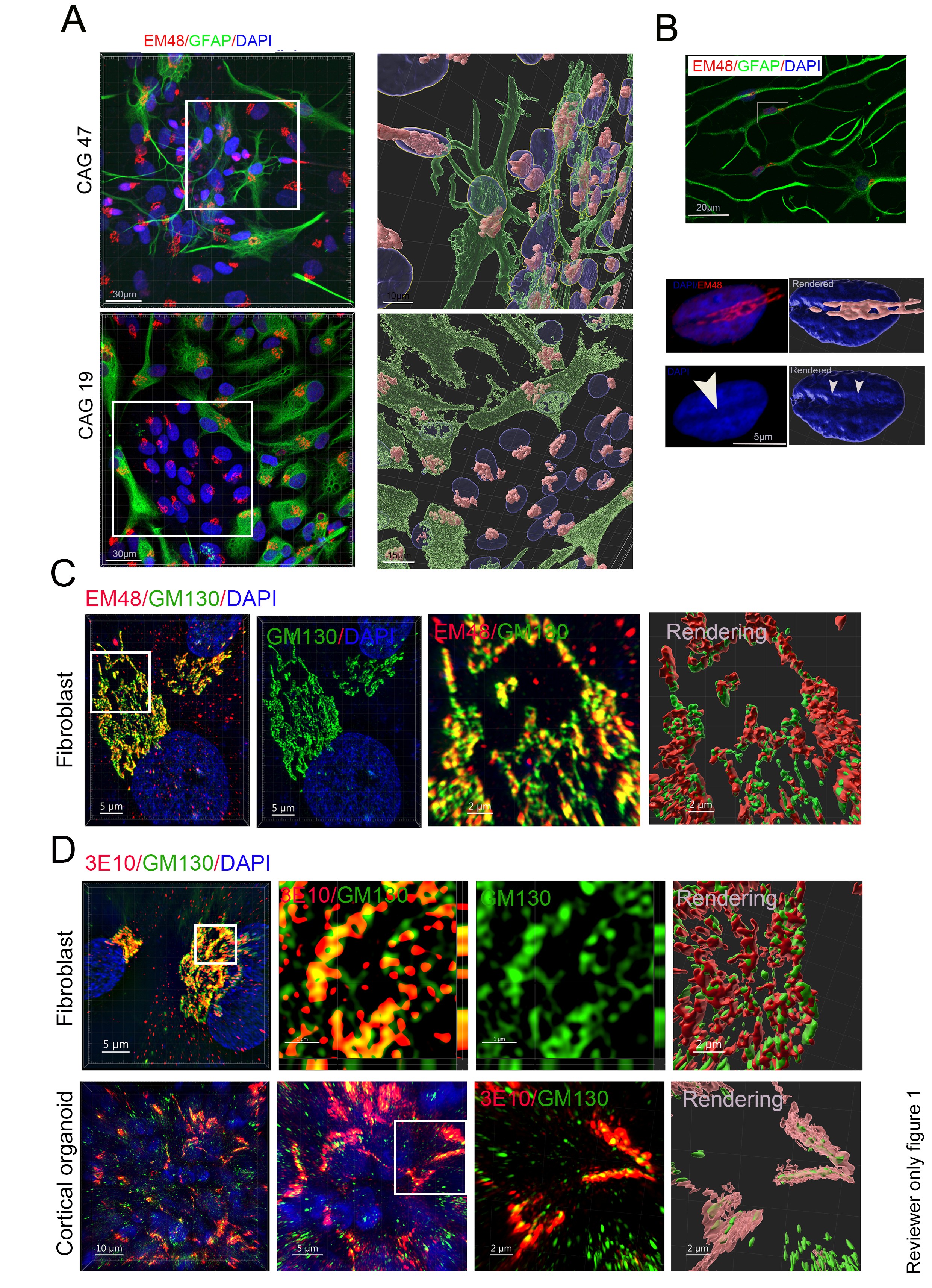
We investigated whether the polyQ assemblies detected by the 3B5H10 antibody contain full-length or large fragments of huntingtin (HTT). To test this, we selected two distinct HTT antibodies: EM48, which binds the first 256 amino acids (excluding the polyQ stretch), and 3E10, which targets the HDA region (amino acids 1171–1177). In patient fibroblasts, the immunostaining patterns for both EM48 and 3E10 were nearly identical to those observed with 3B5H10. These results demonstrate that the polyQ assemblies in fibroblasts are primarily composed of HTT proteins (see Author response image 1). We will include the results of EM48 and 3E10 immunostaining in the revised version.

Author response image 1.

(A) GFAP and EM48 antibodies staining of the astrocytes derived from HD patient and healthy sibling iPSCs showed polyQ assembly in the astrocytes derived from iPSC. (B). The spindle of polyQ assembly formed a dent on the nuclear surface of astrocytes. (C, D) Coimmunostaining of GM130 antibody with 3E10 or EM48 antibody in fibrobalsts revealed that polyQ assemblies contain great amount of HTTs. The middle and right panel are the sectional view boxed region (D) and the boxed region are a magnified part or rendering part (C, D) .

We also check whether the transfected exogenous HTT fragment of the first exon can be recruited into polyQ assemblies. We transfected fibroblasts with three vectors of the HTT first exon containing 19, 23, and 74 CAGs, respectively. The exogenous HTT fragments of the first exon did not significantly recruit into endogenous polyQ assemblies-Golgi complexes of fibroblasts (please refer to Reviewer only figure 5). We will include this part in the revised version.

In the cover letter, we told the editor that we have been studying this structure for over ten years. The results have been stable for over ten years.

Furthermore, the Golgi is identified solely using GM130, a cis-Golgi and ER exit site marker. This raises ambiguity: does polyQ HTT associate with the entire Golgi or only recruit GM130? Could the observed signal correspond to a sub-Golgi compartment?

Thank you for highlighting the precise sub-Golgi localization of GM130 as resolved by electron microscopy. We agree that transmission electron microscopy (TEM) demonstrates GM130 is restricted to the cis-Golgi network, intercisternal regions, and tubular structures, and is absent from the trans-Golgi (Nakamura et al., 1995). Given that individual Golgi cisternae measure approximately 20 nm in width, resolving cis- versus trans-Golgi sub-compartments exceeds the physical resolution limits of our microscopy system. Consequently, GM130 was utilized here as a robust, widely accepted pan-Golgi marker rather than a tool for sub-compartmental differentiation. To specifically evaluate the trans-Golgi network (TGN), we tracked Clathrin+ vesicles, which actively sort at the TGN (Klumperman, 2011). Our Clathrin staining confirms that polyQ assemblies localize to both the cis- and trans-Golgi compartments, as clearly demonstrated in the new lateral view projections provided in revised Figure 4C.

If polyQ HTT is indeed Golgi-associated, several key observations become expected rather than novel. For example, in Figure 4I-M, sensitivity to Brefeldin A is unsurprising, as Golgi structure collapses upon such treatment; in Figure 4N-O, co-fragmentation with the Golgi is expected under Golgi-disrupting conditions.

We agree that our data demonstrate the formation of a functionally coupled polyQ assembly–Golgi complex. Physically and structurally, the dynamics of polyQ assemblies are intrinsically linked to Golgi dynamics under distinct physiological states, including cell cycle progression and energy deprivation. This structural coupling is mediated by ADP-ribosylation factor 1 (ARF1). Specifically, the polyQ tract of HTT interacts with ARFIP2, which is one of the key effector proteins that physically bind active ARF1. Mechanistically, ARF1 is recruited to the Golgi membrane upon GDP-to-GTP exchange catalyzed by guanine nucleotide-exchange factors (GEFs). Consequently, treatment with Brefeldin A (BFA)—which inhibits ARF1 activation—effectively decouples the polyQ assemblies from both intact and fragmented Golgi structures.

Regarding the question of novelty, we define experimental novelty based on generating entirely unprecedented, empirical data that either confirms or redefines biological expectations, rather than evaluating conceptual expectations themselves. We believe the uncovering of this real-time, stimulus-responsive coupling mechanism provides fundamentally novel insights into HTT biology.

(2) 3D rendering

The extensive use of 3D rendering appears unnecessary and, in some cases, misleading. The rendered images do not provide additional insight beyond conventional 2D fluorescence images. Serial 2D fluorescence sections should be more objective in representing the 3D organization.

Thanks for pointing out the 3D rendering. While 3D rendering provides an essential spatial approximation of fluorescently labeled architectures, it offers significantly more precise structural information than conventional 2D or serial section imaging alone (Cao et al., 2023; Han et al., 2021; Hexige et al., 2015). A primary objective of our study was to evaluate these subcellular features within their intact, native three-dimensional context rather than relying solely on two-dimensional cross-sections. Crucially, without complete volumetric rendering, it is mathematically and visually challenging to accurately delineate complex morphological features, such as the nuclear gorge or true intranuclear accumulation. Consequently, 3D volumetric analysis and rendering are entirely indispensable for the accurate interpretation of the structural data presented in this study.

In Figure 2A and Figure 5A, red line features in 3D beige polyQ HTT structures resemble unrelated biological structures, such as vasculature, which is inappropriate.

We would like to clarify that there is no vasculature present within the referenced 3D rendering. The features the reviewer is highlighting are artifacts of the pseudo-coloring used exclusively to mask and visualize the surface tomography. In volumetric 3D rendering, pseudo-colors are assigned strictly to enhance visual clarity and contrast for the reader; they carry no intrinsic biological meaning or cellular identity. Furthermore, from a structural standpoint, the narrow red features in the rendered image are orders of magnitude smaller than true microvasculature. Functional microvessels possess a minimum diameter of 6 to 45 micrometers and exhibit a defined vascular lumen, endothelial cells, a basement membrane, pericytes, and a tunica intima. Therefore, based on both the scale of the image and established histological criteria, these features cannot biologically or structurally represent vasculature.

There is also an inconsistency in rendering. For example, fine mesh-like structures are shown in some figures (e.g., Figure 2A, Figure 4A), whereas others appear as amorphous aggregates (e.g., Figure 5A, Figure S2B), without explanation.

The selection of opacity and color masks in our 3D volumetric reconstructions is systematically chosen to optimize the visual clarity and spatial relationships between intersecting sub-cellular structures. For example, as shown in the fourth and fifth panels, an opaque blue mask was applied to clearly define the outer surface tomography. Conversely, in the third panel, a semi-transparent blue mask was utilized for the nucleus. This transparency is methodologically necessary because a subset of polyQ fragments is embedded within or localized directly inside the nuclear envelope; a transparent mask allows for the unambiguous visualization of these internal structures. Similarly, the inset in Figure 5A illustrates the distinct intranuclear occupancy pattern of polyQ, which also necessitates a transparent nuclear boundary. Collectively, these volumetric rendering strategies provide critical spatial and structural depth that cannot be captured by conventional 2D cross-sections or unconstructed serial imaging.

(3) Quantification of area and volume

The manuscript extensively quantifies the area and volume of polyQ assemblies (e.g., Figure 2B, C and Figure 3B, C, E, G, H). These measurements are not reliable. First, the structures appear filamentous and likely below the diffraction limit. Second, fluorescence signals are broadened by the point spread function (PSF), artificially inflating measured dimensions. Last, even with 3D SIM (~100 nm resolution), fine structural details remain unresolved. Thus, these quantitative measurements lack physical meaning and might not be used to support conclusions.

We appreciate the reviewer’s thoughtful critique regarding the quantification of area and volume. Our measurements are derived from immunofluorescent signals captured via structured illumination microscopy (SIM) and confocal imaging. If the reviewer's concern is that antibody-labeled structures do not perfectly match the absolute physical dimensions of native polyQ assemblies due to the linkage error of the primary-secondary antibody complex, we agree conceptually.

However, our imaging pipeline is optimized to minimize these discrepancies. Our SIM resolution reaches approximately 64 nm. Given that the total observed thickness of the fluorophore-labeled polyQ assemblies exceeds 200 nm, these structures reside well within the detectable range of our super-resolution system, minimizing diffraction-induced overestimation. Regarding the point spread function (PSF) and optical distortion, we emphasize that all comparative quantifications across experimental groups were conducted under identical imaging parameters and thresholds, ensuring a standardized baseline. Furthermore, our acquisition systems (Leica, Nikon, and Zeiss) utilize advanced deconvolution algorithms specifically designed to mitigate PSF-related blur. While we observed that deconvolution yielded negligible baseline improvements when using high-numerical-aperture objectives (63x) or 100x, oil immersion), it validates that our raw high-resolution scanning was already highly optimized.

We acknowledge that an immunolabeled complex is not structurally identical to a naked, pure polyQ tract. Nonetheless, indirect immunofluorescence remains the most robust method to evaluate spatial distribution in situ. Indeed, cryo-EM studies have highlighted that native polyQ tracts are highly flexible and structurally dynamic, making them exceptionally difficult to resolve in their native state (Guo et al., 2018). Intriguingly, we observed that antibody-bound polyQ assemblies remain structurally stable for several weeks with minimal fragmentation, suggesting that antibody binding may structurally stabilize these highly flexible regions. Consequently, indirect immunolabeling provides an indispensable framework for capturing these assemblies within the cellular environment.

(4) Interpretation of structural features (Figure 2A)

Descriptions such as "parallel spindles" and "ring-like assemblies" are not clearly supported by the data. The terminology is ambiguous, and the claimed structures are not discernible. The use of the term "interaction" with the nuclear membrane is also inappropriate. At best, the data suggest colocalization, which itself is not convincingly demonstrated.

Please refer to Fig. 2A (middle upper), Fig. 2F, and Fig. 4C for “parallel spindles”. Please refer to Fig. 5I, J, and Fig.S3C (right panel) for additional clear “ring-like assemblies”. Due to the unique spatial distribution of the 'ring-like assemblies', observing multiple rings within a single spindle is technically challenging. Accordingly, we have tempered our statement in the revised manuscript to accurately reflect this limitation. Furthermore, it is important to note that the visualized structures represent the fluorescent signal from secondary antibodies rather than direct imaging of the proteins themselves. Consequently, we cannot definitively confirm whether this immunostaining pattern precisely replicates the native state of polyQ assemblies within the cellular environment.  

(5) Mitotic fragmentation (Figure 2E)

The conclusion that polyQ assemblies fragment during mitosis lacks proper controls. It is unclear whether these cells exhibited intact "fabric-like" assemblies during interphase, or the observed structures were already fragmented prior to mitosis.

We thought that we had displayed enough non-mitotic cells in this study (Fig. 2A, D, Fig. 4A, F). Most of the cells in this study are non-mitotic cells (G1+S+G2). Thus, we consider the control of non-mitotic cells to be redundant here.

(6) Fixation-induced fragmentation (Figure 2F)

The claim that fixation-induced fragmentation reflects a unique dynamic property of polyQ assemblies is likely an overinterpretation. This phenomenon may simply represent a fixation artifact. Therefore, it cannot be used as evidence for in-cellulo structural dynamics.

By definition, a laboratory artifact refers to any unintended structural detail, distortion, or error introduced by experimental equipment or the preparation process. We contend that the observed phenomenon represents a native chemical characteristic of the HTT polyQ domain inside cells following paraformaldehyde (PFA) fixation, rather than a technical artifact. Similar structural features have been documented by other investigators in tissue samples (Ferrante et al., 1997). A classic textbook example of an artifact is the lamina lucida of the basal lamina, which is artificially generated during electron microscopy tissue processing and does not exist in living tissue. In contrast, the fragmentation of polyQ assemblies occurs naturally both in living cells subjected to stress and during post-fixation processing.

(7) Nuclear localization claims (Figure 5A)

The assertion that polyQ assemblies "almost completely occupy the nucleus" is not supported. The images are more consistent with perinuclear localization, typical of the Golgi region. There is no clear evidence for nucleoplasmic distribution.

Please refer to the rendering image in the upper left inner insert of HD neurons (the blue [transparent] is the nucleus and the pink white is polyQ). The almost complete occupation of the nucleus is crystal clear in these images (rendered inner inserts, upper left). In iPSC-induced HD neurons, it is not only distributed in the nucleus but also in the cytoplasm. Based on your description, you might refer to the cytoplasmic polyQ assemblies but not the nucleus in the rendering image of the upper left (left panel). We will add a label in the revised version for clarity (white arrows for nuclear accumulation). In this manuscript, we have enough figures that clearly show the nuclear accumulation. Please also refer to Fig. 7 and Fig. S2 for additional images of nuclear accumulation.

(8) Drug treatment and data interpretation (Figure 3D-E)

The x-axis in Figure 3E is non-linear, which is inappropriate unless explicitly justified. Furthermore, the rationale for using Onjisaponin F is unclear. What is its known mechanism? Does it affect the Golgi organization? Without this context, observed effects may reflect Golgi perturbation rather than specific effects on polyQ assemblies.

We appreciate the reviewer pointing out Figure 3E. In this experiment, Huntington's disease (HD) fibroblasts were cultured in a low-glucose medium for the first 72 hours, which accounts for the linear trend observed across the first four data points. Following this 72-hour period, the cells were switched to a high-glucose medium and cultured for an additional 48 hours to evaluate subsequent dynamic changes in the polyQ assemblies. To improve visual clarity, we have color-coded these distinct treatment conditions in the revised manuscript, using red to denote low-glucose treatment and green to denote high-glucose treatment.

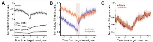
Regarding the choice of Onjisaponin treatment (a concern also raised by another reviewer), Onjisaponin is an active component derived from Radix Polygalae (Yuan Zhi). Previous literature indicates that Onjisaponin B enhances autophagy, accelerates the degradation of mutant α-synuclein and huntingtin in vitro, and activates the AMPK-mTOR signaling pathway (Wu et al., 2013). To optimize our experimental model, we screened multiple variants—specifically Onjisaponin B, D, and F. We determined that Onjisaponin F exhibits remarkably low cytotoxicity while maintaining a robust autophagy-enhancing capacity in both human fibroblasts and iPSC-derived neurons. Consequently, Onjisaponin F was selected for our human cell line experiments (please refer to the Reviewer only image 3). While we did not previously assess Golgi apparatus alterations under Onjisaponin F treatment, we recognize the value of this metric. We are currently evaluating changes to both the Golgi apparatus and neuronal firing rates following Onjisaponin F exposure, and this new dataset will be integrated into our revision.

Reviewer #2 (Public review):

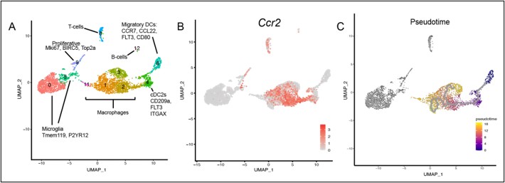
[…] Overall, this work reports a novel polyQ assembly, which was previously reported as a pathogenic factor, has not been reported before for HTT, is related to Golgi activities and vesicular transport, and is dismantled in HD patient cells. The intensive immunostaining and super-resolution scanning are impressive and definitely strengthened by the impact of the findings. The scRNAseq data adds another layer to the observed Golgi impairments and their suggested relationship to Golgi function. The drug testing for polyQ assemblies, especially polyQ assemblies in HD cells, is preliminary. However, the data in this study are enough to support the existence of polyQ assemblies in human cells and their specific relationships with the Golgi apparatus.

We sincerely thank the reviewer for their time, dedication, and insightful evaluation of our manuscript. We agree that the drug screening component represents an initial phase of discovery, and we appreciate the opportunity to clarify this in our text. As the reviewer notes, executing high-throughput or exhaustive drug screenings in human brain organoids is exceptionally resource- and time-intensive due to prolonged culture requirements. We will provide more mechanistic and physiological details of these drug in the future.

Strengths:

In this study, the authors used the cells from a large HD family and fetal/child brain samples to decode the structure of endogenous polyQ assemblies. This part is impressive. The intensive staining and super-resolution scanning are amazing. The spatial relationships of polyQ assemblies with the Golgi apparatus and mitochondria are well illustrated.

Weaknesses:

Although they used healthy sibling cells as a control, an isogenic control (genetic correction of the mutant gene) is lacking. Based on the Golgipathy of mHTT, they did a drug screening. The drug testing for polyQ assemblies is preliminary. More rigorous validation, such as scRNA seq and proteomic analysis, etc., is necessary to reach a systemic conclusion.

References

Barnat, M., Capizzi, M., Aparicio, E., Boluda, S., Wennagel, D., Kacher, R., Kassem, R., Lenoir, S., Agasse, F., Braz, B.Y., et al. (2020). Huntington's disease alters human neurodevelopment. Science 369, 787-793.

Brandstaetter, H., Kruppa, A.J., and Buss, F. (2014). Huntingtin is required for ER-to-Golgi transport and for secretory vesicle fusion at the plasma membrane. Dis Model Mech 7, 1335-1340.

Cao, L., Ma, L., Zhao, J., Wang, X., Fang, X., Li, W., Qi, Y., Tang, Y., Liu, J., Peng, S., et al. (2023). An unexpected role of neutrophils in clearing apoptotic hepatocytes in vivo. Elife 12.

del Toro, D., Canals, J.M., Gines, S., Kojima, M., Egea, G., and Alberch, J. (2006). Mutant huntingtin impairs the post-Golgi trafficking of brain-derived neurotrophic factor but not its Val66Met polymorphism. J Neurosci 26, 12748-12757.

DiFiglia, M., Sapp, E., Chase, K., Schwarz, C., Meloni, A., Young, C., Martin, E., Vonsattel, J.P., Carraway, R., Reeves, S.A., et al. (1995). Huntingtin is a cytoplasmic protein associated with vesicles in human and rat brain neurons. Neuron 14, 1075-1081.

DiFiglia, M., Sapp, E., Chase, K.O., Davies, S.W., Bates, G.P., Vonsattel, J.P., and Aronin, N. (1997). Aggregation of huntingtin in neuronal intranuclear inclusions and dystrophic neurites in brain. Science 277, 1990-1993.

Ferrante, R.J., Gutekunst, C.A., Persichetti, F., McNeil, S.M., Kowall, N.W., Gusella, J.F., MacDonald, M.E., Beal, M.F., and Hersch, S.M. (1997). Heterogeneous topographic and cellular distribution of huntingtin expression in the normal human neostriatum. J Neurosci 17, 3052-3063.

Guo, Q., Bin, H., Cheng, J., Seefelder, M., Engler, T., Pfeifer, G., Oeckl, P., Otto, M., Moser, F., Maurer, M., et al. (2018). The cryo-electron microscopy structure of huntingtin. Nature 555, 117-120.

Han, X., Ma, L., Gu, J., Wang, D., Li, J., Lou, W., Saiyin, H., and Fu, D. (2021). Basal microvilli define the metabolic capacity and lethal phenotype of pancreatic cancer. J Pathol 253, 304-314.

Hexige, S., Ardito-Abraham, C.M., Wu, Y., Wei, Y., Fang, Y., Han, X., Li, J., Zhou, P., Yi, Q., Maitra, A., et al. (2015). Identification of novel vascular projections with cellular trafficking abilities on the microvasculature of pancreatic ductal adenocarcinoma. J Pathol 236, 142-154.

Hickman, R.A., Faust, P.L., Marder, K., Yamamoto, A., and Vonsattel, J.P. (2022). The distribution and density of Huntingtin inclusions across the Huntington disease neocortex: regional correlations with Huntingtin repeat expansion independent of pathologic grade. Acta Neuropathol Commun 10, 55.

Khoshnan, A., Ko, J., and Patterson, P.H. (2002). Effects of intracellular expression of anti-huntingtin antibodies of various specificities on mutant huntingtin aggregation and toxicity. Proc Natl Acad Sci U S A 99, 1002-1007.

Klein, F.A., Zeder-Lutz, G., Cousido-Siah, A., Mitschler, A., Katz, A., Eberling, P., Mandel, J.L., Podjarny, A., and Trottier, Y. (2013). Linear and extended: a common polyglutamine conformation recognized by the three antibodies MW1, 1C2 and 3B5H10. Hum Mol Genet 22, 4215-4223.

Klumperman, J. (2011). Architecture of the mammalian Golgi. Cold Spring Harb Perspect Biol 3.

Ko, J., Ou, S., and Patterson, P.H. (2001). New anti-huntingtin monoclonal antibodies: implications for huntingtin conformation and its binding proteins. Brain Res Bull 56, 319-329.

Legleiter, J., Lotz, G.P., Miller, J., Ko, J., Ng, C., Williams, G.L., Finkbeiner, S., Patterson, P.H., and Muchowski, P.J. (2009). Monoclonal antibodies recognize distinct conformational epitopes formed by polyglutamine in a mutant huntingtin fragment. J Biol Chem 284, 21647-21658.

Liu, Y., Chen, X., Ma, Y., Song, C., Ma, J., Chen, C., Su, J., Ma, L., and Saiyin, H. (2024). Endogenous mutant Huntingtin alters the corticogenesis via lowering Golgi recruiting ARF1 in cortical organoid. Mol Psychiatry.

Miller, J., Arrasate, M., Brooks, E., Libeu, C.P., Legleiter, J., Hatters, D., Curtis, J., Cheung, K., Krishnan, P., Mitra, S., et al. (2011). Identifying polyglutamine protein species in situ that best predict neurodegeneration. Nat Chem Biol 7, 925-934.

Nakamura, N., Rabouille, C., Watson, R., Nilsson, T., Hui, N., Slusarewicz, P., Kreis, T.E., and Warren, G. (1995). Characterization of a cis-Golgi matrix protein, GM130. J Cell Biol 131, 1715-1726.

Owens, G.E., New, D.M., West, A.P., and Bjorkman, P.J. (2015). Anti-PolyQ Antibodies Recognize a Short PolyQ Stretch in Both Normal and Mutant Huntingtin Exon 1. Journal of Molecular Biology 427, 2507-2519.

Paulson, H.L., Bonini, N.M., and Roth, K.A. (2000). Polyglutamine disease and neuronal cell death. Proc Natl Acad Sci U S A 97, 12957-12958.

Shen, M., Wang, F., Li, M., Sah, N., Stockton, M.E., Tidei, J.J., Gao, Y., Korabelnikov, T., Kannan, S., Vevea, J.D., et al. (2019). Reduced mitochondrial fusion and Huntingtin levels contribute to impaired dendritic maturation and behavioral deficits in Fmr1-mutant mice. Nat Neurosci 22, 386-400.

Tousley, A., Iuliano, M., Weisman, E., Sapp, E., Richardson, H., Vodicka, P., Alexander, J., Aronin, N., DiFiglia, M., and Kegel-Gleason, K.B. (2019). Huntingtin associates with the actin cytoskeleton and alpha-actinin isoforms to influence stimulus dependent morphology changes. PLoS One 14, e0212337.

Velier, J., Kim, M., Schwarz, C., Kim, T.W., Sapp, E., Chase, K., Aronin, N., and DiFiglia, M. (1998). Wild-type and mutant huntingtins function in vesicle trafficking in the secretory and endocytic pathways. Exp Neurol 152, 34-40.

Wang, C.E., Tydlacka, S., Orr, A.L., Yang, S.H., Graham, R.K., Hayden, M.R., Li, S., Chan, A.W., and Li, X.J. (2008). Accumulation of N-terminal mutant huntingtin in mouse and monkey models implicated as a pathogenic mechanism in Huntington's disease. Hum Mol Genet 17, 2738-2751.

Wheeler, V.C., White, J.K., Gutekunst, C.A., Vrbanac, V., Weaver, M., Li, X.J., Li, S.H., Yi, H., Vonsattel, J.P., Gusella, J.F., et al. (2000). Long glutamine tracts cause nuclear localization of a novel form of huntingtin in medium spiny striatal neurons in HdhQ92 and HdhQ111 knock-in mice. Hum Mol Genet 9, 503-513.

Wu, A.G., Wong, V.K., Xu, S.W., Chan, W.K., Ng, C.I., Liu, L., and Law, B.Y. (2013). Onjisaponin B derived from Radix Polygalae enhances autophagy and accelerates the degradation of mutant alpha-synuclein and huntingtin in PC-12 cells. Int J Mol Sci 14, 22618-22641.

eLife Assessment

This important study builds on previous work from the same authors to present a conceptually distinct workflow for cryo-EM reconstruction that uses 2D template matching to enable high-resolution structure determination of small (sub-50 kDa) protein targets. The paper describes how density for small-molecule ligands bound to such targets can be reconstructed without these ligands being present in the template. However, the evidence described for the claim that this technique improves the alignment of the reconstruction of small complexes compared to standard techniques is incomplete. The authors could better evaluate the effects of model bias on the reconstructed densities, as suggested by reviewer #1.

Reviewer #1 (Public review):

Summary:

This paper describes an application of the high-resolution cryo-EM 2D template matching technique to sub-50kDa complexes. The paper describes how density for ligands can be reconstructed without having to process cryo-EM data through the conventional single particle analysis pipelines.

Strengths:

Improved insights in which particles contribute to the density of ligands that is absent from the templates are valuable.

Weaknesses:

Although the convenient visualisation of small molecules bound to protein targets of a known structure would be relevant for the pharmaceutical industry, the evidence described for the claim that this technique "significantly" improves alignment of reconstruction of small complexes is incomplete. In a revised paper, the authors are encouraged to better evaluate the effects of model bias on the reconstructed densities.

In the revised version, the refinement of atomic occupancies in the 2DTM-generated maps has been insightful: densities only come back at values ranging from 0.55-0.80, whereas residues included in the template remain at 1, suggesting that the 2DTM-reconstruction does suffer from model bias. Their newly added Omega calculations, which are helpful, also suggest that model bias is present in the 2DTM-based reconstructions. These observations therefore contradict the first subsection heading of the Results, which claims "unbiased reconstruction of omitted residues".

Both the Omega analysis and the refined atomic occupancies provide insights into the "real-space aspect" of the model bias. The question to what extent the model bias affects the map in Fourier space remains unanswered. The authors base some of their claim in the paper on FSC curves in Figures 1b and 3b, but these will suffer from the same model bias. To assess this, I had requested the authors to reconstruct an OMIT map and to assess its resolution using FSCs. The authors have indeed performed a careful reconstruction of an OMIT map, which is currently shown in Figure 5. I liked how they implemented this, as described in detail in the Methods section. However, the measurement of how much model bias is present in this OMIT map by FSC calculations is still pending. This could be done in two ways, and I would encourage the authors to present the results of both in (hopefully a last) revised version of their manuscript. My original suggestion was to calculate a map-to-model FSC for the OMIT map and the full reference. This should be compared with a similar map-to-model FSC on the map where only the ligand was omitted. Alternatively, they can use the cisTEM FSC_uncorr procedure on the OMIT half-reconstructions and compare the resulting curve with the one presented in Figure 1b.

The reason that I am keen to see these FSCs is because high-resolution model bias is a fundamental danger of the 2DTM approach. It will therefore also be in the interest of the authors to quantify the extent to which it happens. For now, I have kept the above public review and short assessment the same as they were, but I will consider raising the assessment after the suggested experiments (which I hope will be relatively easy to do!) are incorporated.

Reviewer #3 (Public review):

Summary:

Due to the low SNR of cryo-EM micrographs necessitated by radiation damage, determining the structure of proteins smaller than 50 kDa is exceedingly challenging, such that only a handful have been solved to date. This work aims to improve the reconstruction of small proteins in single-particle cryo-EM by using high-resolution 2D template matching, an algorithm previously used to locate and align macromolecules in situ, to align and reconstruct small proteins. This approach uses an existing macromolecular structure, either experimentally determined or predicted by AlphaFold, to simulate a noise-free 3D reference and generates whitened projections, crucially including high-spatial-frequency information, to align particles by the orientation with maximal cross-correlation. They demonstrate the success of this approach by generating a 3D reconstruction from an existing dataset of a 41.3 kDa protein kinase that had previously evaded attempts at high-resolution structure determination. To alleviate concerns that this is purely from template bias, they demonstrate clear density at two regions that were not present in the template: 6 residues in an alpha helix and an ATP in the ligand binding pocket. The latter is particularly important for its implications in determining structures of ligand-bound proteins for drug discovery. They also produce a composite omit map from 36 partial-deletion reconstructions spanning the entire protein, demonstrating a reconstruction can be obtained without template bias. Additionally, the authors provide an update to the classic calculation in Henderson 1995 to predict the minimum molecular mass of a protein that can be solved by single-particle cryo-EM.

Strengths:

I am in no doubt that this technique can be used to gain valuable insights into the structures of small proteins, and this is an important advancement for the field. It is complementary to single-particle cryo-EM and provides an extra tool for the experimentalist that may work better in certain cases. For cases where only a small region of the structure is of interest, such as in drug screening, this method provides a simple workflow to screen many structures.

The claim that using high-spatial frequency information is essential for aligning small proteins is a valuable insight. A recent pre-print published at a similar time to this manuscript used high-resolution information in standard ab-initio reconstruction to generate a high-resolution reconstruction from the same dataset, supporting the claims made in the manuscript.

The theoretical section outlined in the appendix is also theoretically sound. It uses the same logic as Henderson, but applies more up-to-date knowledge, such as incorporating dose-weighting and altering the cross-correlation based noise estimation. This update is valuable for understanding factors preventing us from reaching the theoretical limit.

Weaknesses:

The applicability of this technique to more than a single target was not demonstrated. Nor was it compared to more recent strategies for processing SPA data from small molecules, such as Blush regularization or HR-HAIR. Additionally, although the authors have demonstrated convincingly that their method selects a stack of high-quality particles, it is less clear whether it performs better than RELION when using the same stack of particles, particularly in the ATP binding pocket. This places this method as a complementary technique, and whether it outperforms those methods for a wide variety of molecules is yet to be determined. The method presented here also introduces template bias, so only parts of the reconstruction not in the initial template are free of template bias. Producing a full reconstruction through a composite omit map is computationally expensive, meaning that unless this method outperforms modern SPA methods, its major use case will be ligand binding studies instead of 3D reconstructions.

Author response:

The following is the authors’ response to the original reviews.

eLife Assessment

This important study builds on previous work from the same authors to present a conceptually distinct workflow for cryo-EM reconstruction that uses 2D template matching to enable highresolution structure determination of small (sub-50 kDa) protein targets. The paper describes how density for small-molecule ligands bound to such targets can be reconstructed without these ligands being present in the template. However, the evidence described for the claim that this technique “significantly” improves the alignment of the reconstruction of small complexes is incomplete. The authors could better evaluate the effects of model bias on the reconstructed densities.

We have addressed both concerns. Regarding the claim that 2DTM “significantly” improves alignment, the most direct evidence is the controlled comparison in Fig. 3: using the same particle stack and the same reconstruction software (RELION), 2DTM-derived orientations yield a 3.1 Å reconstruction whereas RELION auto-refinement of the same particles yields 3.7 Å. Because the orientations are the only variable, this comparison directly demonstrates that 2DTM produces more accurate alignments.

We further evaluated RELION auto-refinement with initial low-pass filters of 3, 5, 10, and 15 Å (Fig. 3c); the final resolution remained between 3.7 and 4.0 Å across all conditions, indicating that the achievable resolution difference reflects a fundamental distinction between the two approaches. 2DTM directly leverages high-resolution signal in the template during alignment, which is particularly advantageous for small particles.

To assess whether this improvement extends beyond the ligand pocket, we constructed a composite omit map (Fig. 5) assembled from 36 reconstructions, each generated using a template with a different subset of residues deleted. The composite shows that density can be recovered at distributed locations across the kinase, including peripheral and surface-exposed regions further away from the alignment center. Recovery varies across sites, with some regions exhibiting weaker or fragmented density, consistent with local differences in structural heterogeneity and residual alignment error. Together, these results indicate that the orientation estimates support global density recovery rather than being confined to the ligand-binding region.

Regarding model bias, we have strengthened both the quantitative and visual analyses. Specifically, we have (i) updated the template-bias metric Ω in Fig. 4, (ii) added grouped occupancy refinement showing that omitted residues 222–227 refine to 0.55–0.80 (mean 0.72), ATP to 0.61, and Mn to 0.28, while template-included control residues 150–155 remain near 1.0 (0.88–1.00; mean 0.96), and (iii) completed the composite omit map described above. Together, these results provide consistent evidence that densities corresponding to omitted regions are not driven by the template and can be recovered from the data, while template-included regions show some, albeit limited evidence of overfitting, as expected.

Reviewer #1 (Public review):

Summary:

This paper describes an application of the high-resolution cryo-EM 2D template matching technique to sub-50kDa complexes. The paper describes how density for ligands can be reconstructed without having to process cryo-EM data through the conventional single particle analysis pipelines.

Strengths:

This paper contributes additional data (alongside other papers by the same authors) to convey the message that high-resolution 2D template matching is a powerful alternative for cryo-EM structure determination. The described application to ligand density reconstruction, without the need for extensive refinements, will be of interest to the pharmaceutical industry, where often multiple structures of the same protein in complex with different ligands are solved as part of their drug development pipelines. Improved insights into which particles contribute to the best ligand density are also highly valuable and transferable to other applications of the same technique.

Weaknesses:

Although the convenient visualisation of small molecules bound to protein targets of a known structure would be relevant for the pharmaceutical industry, the evidence described for the claim that this technique “significantly” improves alignment of reconstruction of small complexes is incomplete. The authors are encouraged to better evaluate the effects of model bias on the reconstructed densities in a revised paper.

We thank the reviewer for these constructive comments. We have updated the template-bias metric Ω in Fig. 4 and added two further quantitative controls: grouped occupancy refinement of omitted residues and a composite omit map spanning the entire protein. Full details are provided in our responses to Comments 1 and 2 below.

Reviewer #1 (Recommendations for the authors):

Main Comments

(1) For the 1ATP structure: Q-scores for deleted residues/ligands are worse than the Q-scores for residues in the template. This means that the reconstructed map must suffer from template bias. Another indication of this bias is that the density for the ATP (and the omitted residues) appears to be weaker than the density for the residues in the template (although this is not easy to assess from the figures). The authors should perform additional experiments to quantify this bias.

(a) One option could be to do what the X-ray crystallographers call an OMIT map, and omit allresidues, a few at a time, from the template in multiple 2DTM runs. They could then assemble a density map from all the omitted residues together and measure the resolution of the omit map against the known template by FSC.

(b) Another insightful experiment would be to take the various 2DTM reconstructed maps describedin the paper and perform a refinement of the atom occupancies of all residues in the structure. Residues included in the template should refine to values close to 1. In the absence of bias, the occupancies of the omitted residues should be 1 too; if the reconstructed map were completely biased, those occupancies would refine to 0. Therefore, the refined occupancies of omitted residues could perhaps serve as a measure for the amount of bias in the reconstructed map.

We thank the reviewer for these detailed and constructive suggestions. We agree that the lower Q-scores for omitted regions indicate weaker density and that template bias exists at residues that are included in the template. To quantify this more directly, we corrected the template-bias metrics at the omitted region (mask from the full–omit template difference) in Fig. 4.

Following the reviewer’s suggestion, we performed Phenix real-space grouped occupancy refinement against the omit reconstruction using the docked full model. The results are shown in Table. S2. We refined occupancies for the omitted residues (chain E 222–227), ATP, Mn, and template-included control residues (chain E 150–155), while excluding waters. The omitted residues refined to occupancies of 0.55–0.80 (mean 0.72), ATP to 0.61, and Mn to 0.28, whereas the control residues remained near 1.0 (0.88–1.00; mean 0.96). These results indicate substantial recovery of density in the omitted regions, but also some degree of bias.

The substantially lower refined occupancy of Mn²⁺ may reflect genuine partial occupancy in the dataset. While compact features can be especially sensitive to residual alignment error, we cannot conclude from the present analysis that alignment effects alone account for the weak Mn²⁺ density.

Finally, we have constructed a composite omit map to assess density recovery across the protein. We generated 36 omit templates, each deleting ∼10 non-overlapping residues scattered across the structure (including peripheral and surface-exposed regions). For each template, an independent 2DTM search and reconstruction was performed. Local density patches were extracted within 3 Å of the omitted atoms (with neighboring residues excluded as described in Methods) and assembled into a composite map (Fig. 5). The composite map shows that density can be recovered at distributed locations across the protein and is not restricted to the central binding pocket. Recovery is variable across sites, with some regions exhibiting weaker or fragmented density, consistent with local differences in signal-to-noise, structural heterogeneity, and residual alignment error.

(2) The claim that 2DTM leads to “Improved” reconstruction (title) and “alignment and reconstruction [...] can be significantly improved” (abstract) is not supported by the data presented in the paper. The smallest single particle structure to resolutions sufficient for de novo atomic modelling is currently the ACA2 complex, with an ordered mass of less than 40 kDa, which was reconstructed using Blush regularisation in RELION. This paper should be referenced, and statements about single particle analysis (SPA) not working for sub-50 kDa complexes should be toned down. In general, I would say that 2DTM and SPA are not competing techniques, and the paper would be better if it focused on the intrinsic advantages of 2DTM (like ease-of-use for screening of pharmaceutical compounds) and useful findings described that make 2DTM better, e.g., excluding thick ice.

We thank the reviewer for this important perspective and have added the Blush regularization reference Kimanius et al. (2024) to the revised manuscript, noting that the 40 kDa Aca2–RNA complex was reconstructed to 2.5 Å resolution using this approach (at L451). Furthermore, Blush regularization could be applied to reconstructions derived from 2DTM-based particle stacks, and a combination of both approaches may yield further improvements.

We agree that 2DTM and SPA are complementary rather than competing techniques and have revised the manuscript to reflect this. We have also toned down claims in the abstract, which now states that 2DTM “reconstructed a previously intractable ∼43 kDa kinase complex and improved the density of its ligand-binding site” rather than making broad claims about SPA limitations. In the discussion, we now describe 2DTM as broadening possibilities for structural studies of targets “that have remained difficult to reconstruct” rather than implying they are impossible by SPA.

Regarding the intrinsic advantages of 2DTM: beyond ligand screening, the composite omit map (Fig. 5, described in Comment 1) demonstrates that 2DTM-derived orientations support density recovery throughout the entire protein, including peripheral and surface-exposed residues, using roughly an order of magnitude fewer particles than conventional SPA workflows.

(3) Given the uncertainties about the amount of template bias in the reconstructed 2DTM densities, I have trouble interpreting the predictions in Table 1. Where would the 1ATP structure lie in Figure 8? How much bias would there be in a 2DTM reconstruction at SNR n = SNR s? Could the authors perform tests on simulated data to confirm these predictions? At the point of SNR n = SNR s, how would a 2DTM reconstruction look, and what would refined occupancies for deleted residues be?

(This may reflect a misunderstanding on my part, but I don’t really see how the SNR n = SNR s is completely dependent on the number of orientations searched (through Equation 1). In Figure 8, is the full search in a 4k x 4k micrograph, or inside a particle box? And what are the relevant search ranges? Perhaps as a consequence of this misunderstanding, I do not understand how one would decide on the amount of noise in the simulated data for these tests.)

We thank the reviewer for this important question and agree that this point needed clearer explanation. In our framework, is the expected alignment-noise level from maximizing many cross correlations, where N_s is the total number of sampled hypotheses in the 5D search (in-plane angle, out of-plane angles, and x, y shifts), not only the number of orientations. Thus, the relevant search is the per-particle alignment search window (full or constrained), not a full 4k×4k micrograph area.

At SNR_n = SNR_s, the true-match and noise-maxima levels are at a threshold; one could imagine if SNR_s is only slightly larger than SNR_n, the correct pose is favored on average, so with sufficiently large particle numbers real omitted-region density should accumulate, but with residual pose errors that attenuate high-frequency amplitudes (effectively a large positive B-factor). In that regime, sharpening (negative-B correction) can improve visibility once signal is accumulated. Therefore, we expect partial recovery rather than fully unbiased recovery at this threshold, with omitted-region occupancies remaining between 0 and 1 and below template-included controls (consistent with our measured values), and improving as SNR_s − SNR_n and particle number increase. Simulations at this exact threshold would require a very large particle number to achieve sufficient statistics, and we leave this to future work. We have added this clarification to the Supporting Information.

(4) The strong (> 5 sigma!!) and ubiquitous difference densities in Figure 9A imply that the authors have a serious problem with their forward model, which could explain some of the effects of model bias discussed above. I recommend they investigate these differences in detail. It would be good to see negative and positive densities in different colours to understand these differences better. The text speaks about incomplete capture of the solvent background, but the difference densities appear to be of much higher spatial frequencies than those typical for background/solvent effects (e.g., 15-20A). It may thus also be helpful to analyse these differences in Fourier space.

We thank the reviewer for this important point. In our previous analysis, we did not incorporate an appropriate protein mask when generating the difference map, which contributed to widespread residual densities. We have now regenerated the map using the program diffmap.exe (https: //grigoriefflab.umassmed.edu/diffmap) with a protein soft mask and moved it to the Supplementary Information (Fig. Figure 1—figure supplement 4, contour SD = 20). With this controlled setup, the strongest coherent residual densities localize to the omitted ATP pocket and residues 222–227, consistent with recovery of omitted features. We have revised the figure/text accordingly and clarified that remaining diffuse residuals are likely due to forward-model mismatch (including solvent/background representation). We also added to the manuscript that improved template generation may be achieved by incorporating recent methods that learn environment-aware scattering factors directly from experimental cryo-EM maps.

Other Comments

(1) P.1: Alongside reference 2, a reference to the 1.2 Å apoferritin structure from the Stark group should be included.

We have added the reference at L30.

(2) P.2: “commond line tool”

We have corrected the typo.

(3) P.2-3: Robust reconstruction of the ATP binding pocket: Auto-refinements in RELION without alignments do not exist, and corresponding statements need to be removed from the manuscript. If one wants to skip alignments, then there is no refinement left to be done. In that case, one should just perform a reconstruction of the 2 halves (e.g., using relion reconstruct) and then run a standard RELION postprocessing.

We agree with the reviewer and have revised the manuscript accordingly. Technically, RELION’s relion refine with the --skip align flag runs an iterative loop that re-estimates the per-particle noise model (spectral noise σ²) and computes the gold-standard FSC between half-maps, but it does not modify the particle orientations or translations. As the reviewer correctly points out, this is effectively a 3D reconstruction followed by postprocessing, not a refinement. We have updated the text to replace “skip-alignment auto-refinement” with “3D reconstruction without angular refinement” to accurately reflect what was performed.

(4) P.3: What are “first-quadrant p-values” and “three-quadrant p-values”?

We apologize for the ambiguity and now define these terms explicitly in the revised text (with citation to the p-value paper). After transforming z-score and SNR to probit coordinates, “first-quadrant” (1Q) p-values use only candidate points with both coordinates > 0 (i.e., both probit-zscore and probitSNR are positive). “Three-quadrant” (3Q) p-values include candidates where at least one coordinate is > 0 (equivalently, all points except the quadrant where both are < 0).

(5) P.5: In Equation (2), it is unclear what Q means from the main text. Would it be better to leave Equation (2) for the Appendix, and only show Equation (3) in the main text?

Thank you for this suggestion. We kept Equation (2) in the main text to preserve the continuity of the derivation, but we now define Q(k,N_i) explicitly at first use as the normalized exposure-weighting transfer function (following Grant 2015). The detailed derivation and assumptions remain in the Supporting Information.

(6) P.6: “Remaining gaps”: this section considers differences between 200 keV and 300 keV electron beam energies. The main practical effect for cryo-EM data sets is that the current detectors are designed for detecting 300 keV electrons, and their DQE is thus a lot worse at 200 keV. The entire paper doesn’t mention detectors. Perhaps because they are assumed to be perfect, but it is still far from the case.

Also, why were defocus searches not performed if the thickness of micrographs was up to 1500 A?

The conclusion of this section states “Considering all these factors...”, but it then claims standard single particle analysis still remains an outstanding challenge. This concluding statement makes no sense, as this whole section was about 2DTM.

Thank you for this comment. We agree and have revised the text to make these points explicit. First, we now state clearly that detector response (DQE) is generally more favorable at 300 keV than at 200 keV, which contributes to the experimental–theoretical gap. Second, we clarify why we did not perform a defocus search in 2DTM: after CTF/thickness filtering, the retained micrographs are predominantly in the thin-ice regime, so expected defocus spread is smaller, while adding a defocus dimension substantially increases computational cost. We also tested downstream refinement (including CTF/beam-tilt related refinement in cisTEM) and did not observe measurable improvement for this dataset (data not included in the manuscript). Finally, we revised the concluding sentence in this subsection to refer specifically to 2DTM-based alignment limits rather than standard SPA, so the section scope is now consistent.

(7) P.7: Data-driven refinement of AlphaFold3 models: it might be worth pointing out that removing residues a few at a time from AF3 models and checking their reconstructed density by 2DTM would come at a considerable computational cost.

We agree. We have demonstrated residue-level omission validation using the X-ray template via a composite omit map (Fig. 5), confirming that the approach is feasible. We have updated the Discussion to reflect this: extending the composite omit approach to AlphaFold3-based templates remains computationally expensive — each omission design requires an independent 2DTM search and downstream reconstruction — and we present this as an important direction for future work.

(8) Figure 1: What is “full FSC” and what is “particle FSC”?

Thank you for pointing this out. We have clarified the terminology in the figure legend and text using cisTEM and Frealign definitions (Grant et al., 2018). What was previously labeled “Full FSC” is now referred to as the uncorrected FSC (FSC_uncor), computed within a generous mask. “Particle FSC” denotes the solvent-corrected FSC, obtained from FSC_uncor using the mask-volume correction factor f as described in the cisTEM/Frealign framework (Grant et al., 2018).

(9) Figure 3: Why were particles in class 5 discarded? The 2DTM approaches described in this paper are all about carefully selecting good particles, yet now the authors use standard 3D classification to throw away another 156 particles. This seems to be an arbitrary choice. How different would the results have been if these had been included in the reconstruction? Alternatively, did these few particles have any 2DTM metrics that would justify their exclusion?

We thank the reviewer for raising this point. Class 5 contained only 156 particles (∼2% of the dataset). While the 2DTM p-value and SNR metrics provide principled criteria for particle selection, they are not perfect, and a small number of suboptimal particles may still pass these filters. To address the reviewer’s concern, we repeated the reconstruction including all five classes. The resulting map achieved a resolution of 3.7 Å, identical to the reconstruction without class 5, confirming that including these particles does not affect the results. We have clarified this point in the manuscript.

(10) Figure 4C: What are the negative sample thicknesses here? Why use an inset?

The negative sample thickness values are artifacts of the CTF-based thickness estimation algorithm in ctffind5. This algorithm fits oscillations in the 1-D power spectrum arising from the interaction between the CTF and the specimen’s finite thickness (a sinc-modulated envelope). When the ice is very thin or the power spectrum is noisy, the optimizer can converge to a physically meaningless negative value. Of the 2,488 total micrographs across both sessions (after CTF score filtering, 2,314 retained), 136 (∼5.9%) returned negative thickness estimates. We have revised Figure 1—figure supplement 1c (previously Figure 4c) to show only the physically meaningful positive thickness values without the inset, which gives a clearer view of the unimodal distribution peaked near 350–400 Å.

Reviewer #2 (Public review):

Summary:

In this manuscript, Zhang et al describe a method for cryo-EM reconstruction of small (sub50kDa) complexes using 2D template matching. This presents an alternative, complementary path for high-resolution structure determination when there is a prior atomic model for alignment. Importantly, regions of the atomic model can be deleted to avoid bias in reconstructing the structure of these regions, serving as an important mechanism of validation.

The manuscript focuses its analysis on a recently published dataset of the 40kDa kinase complex deposited to EMPIAR. The original processing workflow produced a medium resolution structure of the kinase (GSFSC ∼4.3 Å, though features of the map indicate ∼6-7 Å resolution); at this resolution, the binding pocket and ligand were not resolved in the original published map. With 2DTM, the authors produce a much higher resolution structure, showing clear density for the ATP binding pocket and the bound ATP molecule. With careful curation of the particle images using statistically derived 2DTM p-values, a high-resolution 2DTM structure was reconstructed from just 8k particles (2.6 Å non-gold standard FSC; ligand Q-score of 0.6), in contrast to the 74k particles from the original publication. This aligns with recent trends that fewer, higher-quality particles can produce a higher-quality structure. The authors perform a detailed analysis of some of the design choices of the method (e.g., p-value cutoff for particle filtering; how large a region of the template to delete).

Overall, the workflow is a conceptually elegant alternative to the traditional bottom-up reconstruction pipeline. The authors demonstrate that the p-values from 2DTM correlations provide a principled way to filter/curate which particle images to extract, and the results are impressive. There are only a few minor recommendations that I could make for improvement.

We appreciate the positive assessment. In response to the bias-related concerns raised elsewhere, we have: (i) updated the template-bias metric Ω reported in Fig. 4, (ii) added grouped occupancy refinement showing that omitted residues 222–227 refine to a mean occupancy of 0.72 while template-included control residues remain near 1.0, and (iii) assembled a composite omit map (Fig. 5) from 36 partial-deletion reconstructions spanning the entire protein. These additions are described in the revised Results and in the rebuttal below.

Reviewer #2 (Recommendations for the authors):

(1) On page 3, “Finally, by comparing Figure 2a and b, we observed that deleting IP20 strongly reduced signal at several residues.” Looking at Figure 2a and 2b, it was unclear which residues they were referring to.

We have revised the text to explicitly list the affected residues. In the updated Figure 2, we now label the omitted residues with the lowest backbone Q-scores in the structural views (column 2) and include per-residue backbone Q-score plots (column 4), making the comparison between panels (a) and (b) quantitative. For example, when IP20 is additionally deleted (Fig. 2b), residues Phe54, Gly55, Lys72, Glu127, Glu170, and Asp184 all fall below a backbone Q-score of 0.5, compared with only Ser53 and Glu127 in the within-3 Å deletion alone (Fig. 2a).

(2) Figure 1a. Both the published density map and the text “Template” are gray, but the 2DTM template density map is yellow.

Thank you for catching this inconsistency. We have updated Figure 1a so that the 2DTM template density is now rendered in gray, consistent with the X-ray crystal structure (PDB) coloring. The published single-particle map is shown in wheat and the 2DTM reconstruction in blue, providing a clear three-way color distinction.

(3) Figure 1b. I would recommend the x-axis label of “spatial frequency” instead of “resolution” (which is overloaded). Furthermore, the fact that this is not a GSFSC should be clearly labeled in the figure to prevent confusion with a standard GSFSC.

We agree with both suggestions. The x-axis has been relabeled “Spatial Frequency (1/Å)” in the revised figure. We have also added a note in the figure caption stating that these FSC curves are not gold-standard FSCs, as the reconstruction uses orientations determined by template matching rather than independent half-set refinement.

(4) Figure 2: The usage of the negative sign in the labels “-3 Å”, “-5 Å” to indicate within a given radius is a bit confusing. “Within 3 Å”, perhaps?

Thank you for this suggestion. We have changed the labels in Figure 2 from “−3 Å” and “−5.5 Å” to “Within 3 Å” and “Within 5.5 Å.” We have also added a fourth column to Figure 2 showing per-residue backbone Q-scores for each deletion experiment, with omitted residues distinguished by color and marker shape. The residues with the lowest backbone Q-scores among the omitted set are circled in red and correspond to the labeled residues in the structural views.

(5) Figure 4c: Why does the sample thickness histogram go to negative values (-20,000 A)?

As noted in our response to Reviewer 1, the negative thickness values are artifacts of the ctffind5 thickness estimation, which fits a sinc-modulated envelope to the 1-D power spectrum. For micrographs with very thin ice or noisy power spectra, the fit can converge to unphysical negative values. These account for ∼5.9% of micrographs. We have revised Figure 1—figure supplement 1 (originally Fig. 4c) to display only positive thickness values, removing the inset and providing a clearer histogram.

(6) Figured 4d: Should the label be “(Before Filtering)” instead of After?

Yes, thank you for catching this. The original Figure 4d was mislabeled—it showed particle counts before filtering but was titled “After Filtering.” We have corrected the labels: Figure 1—figure supplement 1d (originally Fig. 4d) now reads “Before Filtering” and Figure 1—figure supplement 1e (originally Fig. 4e) reads “After Filtering.”

(7) Supplementary Note 1: Please provide units for d, p, D, and k max in equation S4 and the preceding text.

We have added units to the text preceding Eq. S4: d = 1/k_max is the high-resolution alignment limit (Å), k_max is the maximum spatial frequency (Å ⁻¹), p = d/2 is the ideal pixel size (Å/pixel), and D is the particle diameter (Å).

(8) What does the map-model FSC look like with the template as the model vs. the AF3 structure as the model?

We have computed the map–model FSC for both the X-ray crystallographic template (PDB 1ATP) and the AlphaFold3-predicted template against their respective 2DTM reconstructions (Fig. Figure 6—figure supplement 1). Both curves cross the FSC = 0.143 threshold at ∼2.3 Å. We note that the map–model FSC in this context should be interpreted with caution, because the vast majority of the structure lies outside the omitted region and is present in the template, so template bias in those regions will dominate the map–model FSC and obscure differences in the small omitted region.

Reviewer #3 (Public review):

Summary:

Due to the low SNR of cryo-EM micrographs necessitated by radiation damage, determining the structure of proteins smaller than 50 kDa is exceedingly challenging, such that only a handful have been solved to date. This work aims to improve the reconstruction of small proteins in single-particle cryo-EM by using high-resolution 2D template matching, an algorithm previously used to locate and align macromolecules in situ, to align and reconstruct small proteins. This approach uses an existing macromolecular structure, either experimentally determined or predicted by AlphaFold, to simulate a noise-free 3D reference and generates whitened projections, crucially including high-spatial-frequency information, to align particles by the orientation with maximal cross-correlation. They demonstrate the success of this approach by generating a 3D reconstruction from an existing dataset of a 41.3 kDa protein kinase that had previously evaded attempts at high-resolution structure determination. To alleviate concerns that this is purely from template bias, they demonstrate clear density at two regions that were not present in the template: 6 residues in an alpha helix and an ATP in the ligand binding pocket. The latter is particularly important for its implications in determining structures of ligand-bound proteins for drug discovery. Additionally, the authors provide an update to the classic calculation in Henderson 1995 to predict the minimum molecular mass of a protein that can be solved by single-particle cryo-EM.

Strengths:

I am in no doubt that this technique can be used to gain valuable insights into the structures of small proteins, and this is an important advancement for the field. The ability to determine the structure of ligands in a binding site is particularly important, and this paper provides a method of doing that which outperforms traditional single-particle cryo-EM processing workflows.

The claim that using high-spatial frequency information is essential for aligning small proteins is a valuable insight. A recent pre-print published at a similar time to this manuscript used high-resolution information in standard ab-initio reconstruction to generate a high-resolution reconstruction from the same dataset, supporting the claims made in the manuscript.

The theoretical section outlined in the appendix is also theoretically sound. It uses the same logic as Henderson, but applies more up-to-date knowledge, such as incorporating dose-weighting and altering the cross-correlation-based noise estimation. This update is valuable for understanding factors preventing us from reaching the theoretical limit.

Weaknesses:

Given that this technique creates template bias, only parts of the reconstruction not in the template can be trusted, unlike standard single-particle processing, where the independent half-maps from separate, ab initio templates are used to generate a 3D reconstruction. Although, in principle, one could perform the search many times such that every residue has been omitted in at least one search, this will be extremely computationally intensive and was not demonstrated in this manuscript. It is therefore currently only realistically applicable when only a small portion of the sub-50 kDa protein is of interest.

The applicability of this technique to more than a single target was also not demonstrated, and there are concerns that it may not work effectively in many cases. The authors note in the results that “the ATP density was consistently recovered more robustly than nearby residues” and speculate that this may be because misalignments disproportionately blur peripheral residues. Since the region of interest in a structure is not necessarily in the center, this may need further investigation. The implications of this statement may also be unclear to the reader. For example, can this issue be minimized by having the region of interest centered in the simulated volume?

In Figure 3, the authors demonstrate that it is not solely improved particle filtering and a noise-free reference that improves alignment, but that the high spatial frequency information is important. This information is very valuable since it can be applied to other, more standard methods. However, this key figure is not as clear or convincing as it could be. The FSC curves are possibly misleading, since the reduced resolution could be explained by reduced template bias when auto-refining with a map initially low-pass filtered to 10 A. Moreover, although the helix reconstruction does look slightly better using the 2DTM angles, the improvement in density for ATP in the binding pocket is not clear. A qualitative argument only clear in one out of two cases is not as convincing as a quantitative metric across more examples.

We address these concerns in three ways: (i) we quantify template bias using Phenix real-space grouped occupancy refinement: omitted residues 222–227 refine to occupancies of 0.55–0.80 (mean 0.72) and ATP to 0.61, while template-included control residues 150–155 remain near 1.0 (mean 0.96), confirming that recovered density is genuine rather than a template artifact; (ii) we have now completed a composite omit-map experiment (Fig. 5), in which 36 partial-deletion templates, each omitting ∼10 non-overlapping residues, were used to perform independent 2DTM searches and reconstructions; local density patches from all 36 reconstructions were assembled into a composite map showing density recovery at distributed locations across the protein, including peripheral and surface-exposed regions, although recovery is variable across sites; and (iii) we have expanded the discussion to clarify that, while the primary scope of this work is omitted-region validation for the ligand-binding site, the composite omit-map result demonstrates that the approach generalizes beyond the central pocket.

Reviewer #3 (Recommendations for the authors):

In addition to the comments on the public review, I have some more specific suggestions that could improve the manuscript.

(1) Another recent pre-print posted on BioRxiv shortly before this manuscript (Kim et al. Highresolution ab initio reconstruction enables cryo-EM structure determination of small particles) determined a high-resolution structure of the same protein from the same dataset, as well as determining the structures of other small proteins. Since both manuscripts rely on high-spatial frequency information, I think that the paper strengthens the claims in this manuscript and should be cited.

We thank the reviewer for this suggestion. We agree that the recent preprint by Kim et al. strengthens the relevance of high-spatial-frequency information for small-particle cryo-EM reconstruction. We have now added this work to the revised manuscript and included a brief discussion comparing its ab initio strategy with our 2DTM-based approach.

(2) The claim in the abstract that “we were able to reconstruct previously intractable targets under 50 kDa and improve the density of the ligand-binding sites in the reconstructions” should be altered to make it clear that this is only a single previously intractable target.

We agree. The revised abstract now reads “. . . we reconstructed a previously intractable ∼43 kDa kinase complex and improved the density of its ligand-binding site” making clear that a single target is demonstrated in this work.

(3) Q-scores in the manuscript were sometimes used to quantify the improvement in map to model fit for the ATP binding pocket, but never for the 6 residues of the alpha helix. They were also not reported in every case for the ATP-binding pocket. This could lead a reader to think it is only being reported when the Q-score matches the expectation. For transparency, I would suggest either using Q-scores in every comparison or in no cases and simply relying on the qualitative result.

We agree with the reviewer. In the revised manuscript, we now report Q-scores consistently for both ATP and residues 222–227 across all conditions: individual residue Q-scores for the omitted residues 222–227 in Fig. 1 are reported in the main text and figure caption; per-residue backbone Q-score plots for all deletion experiments in Fig. 2 are shown as the fourth column of each panel; Fig. 3 (RELION reconstruction) does not include Q-scores as the focus is on orientation accuracy rather than map-model fit; and average Q-scores for all four particle selection conditions in Fig. 4 are listed in Figure 4—source data 1.

(4) The sigma values used for viewing the maps should also be stated in several figures, particularly Figure 3 and Figure 6.

We have added contour levels (σ) to the captions of Fig. 3 and Fig. 4 (originally Fig. 6) in the revised manuscript.

(5) I have a slight concern about how well this method applies away from the region centered in the alignment. If parts on the periphery of the structure are removed, do these also reconstruct? Is it required that the omitted region be centered in the simulation of the 3D volume for each alignment? If so, this should be clearly stated.

2DTM determines particle orientations by matching the full projected template to the image, so alignment is driven by the global structure rather than a localized region. As a result, the recovered orientations define the reconstruction throughout the entire particle, not only near the center. The omitted region does not need to be centered in the template volume. Any region of the protein can be omitted and its density evaluated after reconstruction.

To directly test whether peripheral regions are recovered in the same manner as central ones, we performed a composite omit-map experiment. We generated 36 omit templates, each deleting ∼10 non-overlapping residues distributed across the entire protein, including peripheral and surface-exposed regions. For each template, an independent 2DTM search and reconstruction was performed. Local density patches corresponding to the omitted regions were then extracted and assembled into a composite map (Fig. 5). The resulting map shows density at distributed locations across the protein, indicating that density recovery is not restricted to regions near the alignment center and that peripheral regions can be reconstructed under the same alignment framework, although the quality of recovery varies across sites.

(6) I was confused by the difference between the FSCs in Figure 1 and Figure 3. I understand Figure 1 is from cisTEM and Figure 3 from RELION, but I expected the unmasked FSC and full FSC to be similar. Do the authors have any insights into why there is such a large difference? I would also consider removing the FSCs in Figure 3, since the reduced resolution may only be due to reduced template bias, meaning including this may be misleading.

Thank you for raising this point. The apparent discrepancy arises from multiple differences between the two figures: different FSC definitions, different half-maps (reconstructed with different software and slightly different particle sets), and different masks.

In cisTEM (Fig. 1), two FSC curves are reported: the uncorrected FSC (FSC_uncor), measured within a spherical mask, and the “Particle FSC”, which applies an analytical solvent-fraction correction (Grant et al., 2018) to account for solvent dilution within the mask. The Particle FSC crossed the 0.143 threshold at ∼2.6 Å, whereas FSC_uncor crossed at ∼3.0 Å. In Fig. 3, RELION postprocess applied phase-randomization correction with a soft mask, yielding ∼3.1 Å. However, the Fig. 3 FSC was computed on different half-maps (RELION skip-alignment reconstruction of 7,197 particles after 3D classification) with a different mask.

To directly compare the two packages, we computed the FSC on the same cisTEM half-maps using both methods (Figure 3—figure supplement 1). The cisTEM Particle FSC (spherical mask + solvent correction) gave ∼2.6 Å, while RELION image handler with a tight 3D protein mask gave ∼2.7 Å. These two approaches converge to a similar resolution through different mechanisms: cisTEM compensates for a generous spherical mask using the solvent-fraction correction, while RELION uses a tight mask that excludes most solvent directly. This confirms that when the same half-maps are used, the two packages give consistent results and the apparent discrepancy between Figs. 1 and 3 is primarily due to differences in the reconstruction and particle set, not the FSC calculation.

We agree with the reviewer that the FSC values in Figure 3 should be interpreted with caution. In this case, the particle orientations are not independently refined but are instead inherited from the 2DTM alignment, so the two half-maps are not strictly independent. We have added clarifying language in the revised manuscript to make this point explicit (Fig. 1 caption).

(7) I would also like to see how RELION auto-refinement performs with different low-pass filtering. This could strengthen the argument that high-resolution information is necessary from the start to successfully align small particles.

We thank the constructive suggestion from the reviewer. We performed RELION auto-refinement on the same 7,197-particle stack using different initial low-pass filter resolutions (--ini high) of 3, 5, 10, and 15 Å. The resulting post-processed resolutions were:

Author response table 1.

The results show that varying the initial low-pass filter has minimal effect on the final resolution. This is expected because RELION uses a gold-standard, maximum-likelihood framework in which the resolution used for alignment is determined iteratively from the data via a probability distribution, rather than being fixed by the initial reference. After the first iteration, the reference is updated from the data, and higher-resolution information is incorporated only to the extent supported by the definition of the current reconstruction. Consequently, differences in the initial low-pass filter have limited impact on the final refinement outcome.

This behavior contrasts with 2DTM, where alignment is performed by direct cross-correlation against a fixed template. In this case, high-resolution features in the template contribute directly to the scoring function and can improve alignment accuracy.

To directly test the importance of high-resolution information for 2DTM alignment, we performed an additional experiment in which 2DTM was run on bin4x images (2.234 Å/pixel), and the detected particle coordinates were used to extract particles from the corresponding bin2x images (1.117 Å/pixel) for reconstruction. Despite using the same bin2x images for reconstruction, the bin4x-aligned particles yielded a map in which ATP density was lost and backbone density for residues 222–227 was visibly degraded compared to the bin2x-aligned reconstruction (Fig. Figure 1—figure supplement 3). This demonstrates that access to high-spatial-frequency information during template matching is critical for accurate alignment of small particles.

(8) The caption in Figure 3 should be more descriptive about what is being shown in each panel.

We have substantially expanded the Figure 3 caption. It now describes each panel explicitly: (a) 3D classification results with particle counts, percentages, and per-class resolutions; (b) side-by-side comparison of reconstructions using 2DTM orientations versus RELION auto-refine, including full maps, zoomed binding-pocket views with the atomic model overlaid, orientation distributions, and FSC curves with reported resolutions; and (c) a table of RELION auto-refinement resolution as a function of the initial low-pass filter setting. We also added a new panel (c) showing that including all five classes yields the same 3.7 Å resolution, addressing the concern about Class 5 exclusion.

(9) Figures 4 and 5 may be better suited as supplementary figures.

We agree. Figures 4 and 5 have been moved to the Supplementary Information in the revised manuscript.

(10) In Figure 4c, it is difficult to understand why the thickness distribution plot goes negative, especially to such a high magnitude as 1.5 microns.

We agree this was confusing. The negative values are fitting artifacts from ctffind5’s thickness estimation, which fits a sinc-modulated envelope to the power spectrum. When the ice is very thin or the spectrum is noisy, the optimizer can converge to unphysical negative values (affecting ∼5.9% of micrographs). We have revised Figure 1—figure supplement 1c (previously Figure 4c) to show only positive thickness values, which now clearly displays the unimodal distribution peaked at 350–400 Å.

(11) In Figure 5d, the micrograph looks a lot like a cross-grating grid used for calibration instead of crystalline ice or a fractured film.

We agree. We have updated the caption for Figure 1—figure supplement 2d (originally Figure 5d) to read “Cross-grating calibration grid”

(12) Figure 6 was very surprising to me if I am interpreting it correctly. It is not stated in the caption what omega is, but I am assuming it is a measurement of template bias. It is very surprising that the template bias drops when using more particles by reducing the p-value from 8.0 to 7.0. This goes against what I understood from Lucas et al. 2023, so I am curious as to why this is the case.

We thank the reviewer for this question and apologize for the unclear presentation. We have revised Fig. 4 (previously Figure 6) and its caption to define Ω explicitly and updated the Ω values. We also identified that the mask used in the original computation was too loose; the revised mask is now constrained to the omitted region only (ATP, Mn²⁺, and residues 222–227), derived from the difference between the full and omit templates and shown in Figure 4—figure supplement 1. Ω is adapted from the template-bias metric introduced in (Lucas et al., 2023) and measures how much of the density in the omitted region is attributable to using the full template rather than the omit template. Specifically, for each particle selection condition we reconstruct two maps using orientations and particles derived from independent 2DTM searches with the full and omit templates (V_full and V_omit, respectively). Ω is the fractional reduction in density within the omission mask: . In the revised Fig. 4, Ω increases from 46% (p-value = 8.0) to 48% (p-value = 7.0), consistent with the expectation that including more, lower-quality particles increases the relative contribution of the template to the reconstruction. The Ω values are 48% for the SNR = 7.5 and 53% for the tilt conditions.

(13) It would be useful if the in-house Python script used to calculate template bias could be made publicly available.

We agree. The template-bias calculation (measure-template-bias) is now included in the publicly available Python package at https://github.com/kekexinz/2DTM_postprocess_tool, and can also be accessed in the official cisTEM repository at https://github.com/timothygrant80/cisTEM. The package also contains the extract-particles and filter-particles tools described in the Methods section.

(14) The p-value used is said to be a three-quadrant p-value instead of a one-quadrant p-value. Although I assume this is simply replacing an ‘and’ statement with an ‘or’ statement, the exact difference could be made clearer to the reader.

We have now defined these terms explicitly in the revised Methods. After probit transformation of z-score and SNR, the first-quadrant (1Q) p-value requires both values to be > 0 (logical AND), whereas the three-quadrant (3Q) p-value requires at least one to be > 0 (logical OR). The 3Q criterion is therefore looser, retaining more candidates—which is beneficial for small targets that may score well on one metric but not both.

(15) I was, perhaps naively, surprised that z-scores could not be used. It was my understanding that by removing the rotationally invariant component from the cross-correlation, the z-score would down-weight low-resolution information compared to the cross-correlation. Given that the manuscript suggests low-resolution alignment can cause getting stuck in local minima, this is surprising to me. The authors note it led to the rejection of most particles; were there simply too many false positives when a lower threshold was used?

The reviewer is correct that subtracting the angular mean removes the rotationally invariant component of the cross-correlation. However, the resulting z-score primarily measures how strongly a specific orientation stands out relative to other orientations. In other words, it reflects the orientation discriminability (closely related to Fisher information) rather than the absolute correlation strength. For small particles the cross correlation often varies only weakly across orientations, so CC_max− CC_avg remains small even when the absolute correlation is significant. As a result, using the z-score alone as a selection criterion led to the rejection of many true particles.

Theoretical Section Improvements

(a) The discussion on beam-induced motion could be improved by separating it into initial motion (e.g., cryo-crinkling, buckling) that can be eliminated through grid design, and pseudo-Brownian motion, which cannot. Pseudo-Brownian motion will become much more significant for small proteins (based on reference 5, for a 10 kDa protein, this would be a MSD of ∼0.1 A 2/e−/A 2, or a B-factor of over 2 A 2/e−/A 2), and Bayesian Polishing is unlikely to correct this perfectly, given that it imposes a smoothness of motion between nearby particles. The impact of not correcting for this could be quantified more explicitly.

We thank the reviewer for this helpful suggestion. As noted, pseudo-Brownian motion of particles within irradiated ice introduces stochastic displacements that accumulate with dose and are expected to be more significant for small particles. Based on the analysis in (Mcmullan et al., 2015), and scaling with particle size, this effect can be aproximated as a dose-dependent mean-squared displacement (MSD) of ∼0.1 Ų per (e⁻/Ų) for a ∼10 kDa particle. Over a typical total exposure of 40–60 e⁻/Ų, this corresponds to an accumulated RMS displacement of ∼2–2.5 Å, sufficient to attenuate high-resolution signal.

In practice, such motion acts as an additional high-frequency attenuation in Fourier space, analogous to an envelope function, reducing the coherent signal available for template matching. While Bayesian polishing can partially correct beam-induced motion, it assumes spatially smooth trajectories between nearby particles and therefore may not fully compensate for stochastic, particle-specific motion.

Within the theoretical framework presented here, this effect can be interpreted as an additional frequency-dependent damping of the signal (B-factor). Its primary consequence would be to reduce the effective signal-to-noise ratio at high spatial frequencies and therefore shift the detectable molecular-weight limit somewhat upward, without altering the structure of the derivation. We have added text in the manuscript to clarify this point and to indicate the expected magnitude of this effect.

(b) The inclusion of inelastic scattering assumes an energy filter is being used, and this should be clearly stated.

We have added this clarification in the inelastic scattering paragraph of the Supplementary Information.

(c) The reasons for not including other factors, such as DQE and the temporal and spatial coherence envelope functions, could be stated.

We have added a note in the dose-weighting section clarifying that these instrument-dependent attenuation factors were not explicitly included, and that they could be incorporated as additional frequency-dependent weighting terms without changing the structure of the derivation.

(d) The flexibility and heterogeneity in protein structures, especially at high spatial frequencies, must also be a reason for a gap from experiment to theory, but this is not clearly stated.

We agree. We have added a statement in the “Remaining gaps” section noting that structural flexibility and conformational heterogeneity act as an additional envelope that attenuates high-resolution signal relative to the rigid-particle model assumed in our derivation.

Additional Minor Comments

(15) It is noted in the discussion that 2DTM-based single-particle alignment simplifies the processing pipeline. Although true, I think stating the computation time would be useful for the reader.

We have added computation times to the Discussion. For a typical single-particle dataset of ∼2,000 micrographs (5k × 4k pixels), a 2DTM search without defocus refinement completes in approximately one day on 64 NVIDIA A6000 GPUs. Once particles are located with their orientations and positions, a single 3D reconstruction is sufficient without further refinement, eliminating the iterative 2D classification, ab initio modeling, 3D classification and refinement steps of a conventional pipeline.

(16) There are some formatting issues with e−/A 2, sometimes losing the minus sign.

Thank you for catching this. We have corrected all instances to consistently use e⁻/Ų throughout the manuscript.

eLife Assessment

This is an important study that applies a new chromatin profiling technique to the study of cellular responses to low oxygen. The authors provide convincing evidence for distinct kinetic phases of the response and identify many new putative regulators of the response. This work will be of broad interest to those studying low oxygen responses and transcriptional regulation.

Reviewer #1 (Public review):

Summary:

The manuscript by Singh et al. presents an application of MOA-seq to better define transcriptional control underlying the hypoxia response in human endothelial cells. This group's previously described MOA-seq technique allows for precise, identity-agnostic mapping of occupied sites of DNA-binding proteins across the epigenome and over time. Here, they applied MOA-seq to HUVECs under normal oxygen conditions or variable lengths of hypoxia treatment, comparing changes in occupancy over time and associating these changes with corresponding transcriptome alterations. This approach revealed thousands of dynamically occupied sites comprising 10 major kinetic clusters that appear to define distinct subsets and phases of the hypoxia response. Analysis of DNA motifs in these dynamically occupied regions captured the known major roles of HIF1A in the hypoxia response and also implicated new HIF1A-associated regulators. Importantly, they also identified many potential HIF1A-independent candidate TFs that act at HREs, which has been an outstanding question in the field. Additionally, this study identified ~7K additional sites not previously defined as regulatory elements by ENCODE.

Strengths:

Overall, this study is well executed and described, providing new biological insights as well as a rich data resource for the field. As MOA-seq was previously developed for use in plants, this work demonstrates the application of this method in mammalian cells and highlights its utility in identifying new potential regulatory sites not captured by DNase-seq or ATAC-seq. The conclusions made by the authors are well supported by the results, with the caveat that extensive use of DNA motif identification and ontology analyses invariably leads to some uncertainty regarding factor identity and gene network properties.

Weaknesses:

There are several areas where the clarity of presentation could be improved:

(1) Given the importance of the methodology, the methods section needs more detail on how the extent of MNase digestion is chosen to achieve optimal results with MOA-seq. This is described to some extent in the description of control library preparation, but not for the experimental samples.

(2) The abstract describes this approach as "native cistrome profiling" but this is misleading since formaldehyde fixation is used.

(3) Species- and field-specific jargon and abbreviations need to be clarified on first usage. For example, on page 9: "Downsampling analysis was carried out for two sets of published reference peaks; the CTCF cCRE peak midpoints and for the ERG motif under the ERG ReMap ChIP-seq peaks." The different categories of cCREs were not clearly defined, nor will it be clear what the term ReMap refers to for those outside the field. The sentence after this refers to IDR, which also should be defined.

(4) Figure 4C: Are these motifs examined under MOA sites specifically or anywhere in the genes in question?

(5) Figure 5B shows that up-DEGs with diff-MOA footprints tend to show more losses of footprints. Do the authors interpret this as a loss of repressor binding?

Reviewer #2 (Public review):

Summary:

Singh et al. apply MOA-seq to map transcription factor occupancy genome-wide in HUVECs across a hypoxia time course. The study provides a well-validated, high-resolution view of cistrome dynamics and identifies both HIF1A-associated and independent regulatory programs.

Major Comments:

Methodological validation is strong. MOA-seq's ability to map protein-bound DNA at near-nucleotide resolution without factor-specific antibodies is a genuine advance, and the cross-validation against independent ChIP-seq and ENCODE datasets is convincing. As noted, future work with additional biological replicates could further strengthen confidence in the smaller kinetic clusters.

Imaging-based validation would strengthen the key biological claims. The kinetic clustering and pathway enrichments are computationally inferred. Orthogonal approaches, for example, live-cell fluorescence imaging of HIF1A nuclear translocation to confirm the proposed temporal binding waves, would provide independent experimental support.

eLife Assessment

This paper addresses a key question regarding the molecular mechanisms underlying GABA and glutamate release from co-releasing neurons projecting from the entopeduncular nucleus (EPN) to the lateral habenula (LHb) in mice. The authors conclude that the two neurotransmitters are released from separate vesicle pools and rely on distinct molecular machinery; these conclusions contrast with previous functional studies at the same synapse, suggesting that GABA and glutamate are co-packaged within the same vesicles. The study employs useful electrophysiological and imaging approaches, however, a key limitation is the use of Cre lines that also label a purely glutamatergic EPN population projecting to the LHb. This inadequate methodology complicates the interpretation of the data and weakens the central conclusions regarding neurotransmitter co-release mechanisms.

Reviewer #1 (Public review):

Summary:

White et al. explore the role of synaptotagmin isoforms in mediating neurotransmitter release from EPN terminals in the LHb. The authors show a relatively high expression of Syt2 and Syt3 in the EPN relative to other Syt isoforms. The authors then perform a series of experiments to show that Syt2 preferentially regulates glutamatergic transmission while Syt3 regulates GABAergic transmission.

Strengths:

Interesting, timely topic.

Weaknesses:

While interesting, the study is rather preliminary. There are a number of issues the authors need to address.

Reviewer #2 (Public review):

Summary:

This is an important study of the molecular mechanisms of GABA vs. glutamate release by coreleasing neurons that project from the EPN to LHB. The conclusion is that separate pools of vesicles release each transmitter and use different molecular machinery to do so. This is in contrast to and in disagreement with functional studies of the same synapse that conclude that the transmitters are copackaged.

As detailed below, the study has a major flaw. It uses an incorrect Cre line, which is also expressed in a purely glutamatergic population in the EPN that also projects to the LHB. In addition, there is little quantification and validation of important tools and no histological confirmation of the sites of expression of viral-encoded proteins.

Strengths:

The strength of the study is in the importance of the question addressed and in the ambition of the tools used.

Weaknesses:

(1) The study uses Vglut2-IRES-Cre mouse to gain control over EPN to LHB projections. However, as has been shown by several groups, this line is not exclusive to the EPN co-releasing population. It is also expressed in glutamatergic EPN PV neurons that project solely to the EPN. Therefore, all of the studies here are contaminated with analysis of a purely glutamatergic Vglut2+ projection. This calls into question all the conclusions about the differential localization and function of synaptic proteins.

(2) It is unclear from the paper, but it seems that some experiments may have been done with no Cre control, which likely led to contamination in neighboring brain regions, some of which project to LHB as well.

(3) Histology: There is no histology shown for the mice used in the study. This is a crucial point. We need to see that the injection was clean and specific for each mouse used in the study (although, given the use of Vglut2-Cre, it cannot be specific to the coreleasing population). Whole-brain histology is necessary.

(4) ASO KO: Unfortunately, there is little validation of the ASO KO. The effects shown in Figure S2 show a very small effect, if any. There appear to be no statistics. The functional effects in the main figure are also relatively subtle.

(5) Other concerns: There are many typos and errors, including in important claims.

eLife Assessment

The authors have presented a study which addresses a recognised gap in the literature, the emergence of the neural correlates of cognitive and affective empathy in children; they introduce a task for measuring both positive and negative empathy in a relatively large group of children aged 3-5. The task was combined with functional near-infrared spectroscopy to examine brain regions involved in the task. The findings are interpreted as providing evidence for the earlier emergence of cognitive than affective empathy. The study represents a valuable contribution to understanding the development of cognitive function, but in its current form, the strength of support for the conclusion is incomplete due to limited support for the comparison to the adult literature and a need to more clearly justify the pre-selected brain regions, their links to empathy and the justification of the hypotheses.

Reviewer #1 (Public review):

Public Review

This paper presents an fNIRS neuroimaging study with a relatively large sample of preschool children (aged 3-5) that measures both positive and negative empathy within a single task. Children watch emotional events and are asked questions about both their own emotions and the emotions of others, allowing the authors to distinguish between affective and cognitive empathy. The authors propose "foundational" models of affective and cognitive empathy and argue that their findings support the idea that cognitive empathy emerges before affective empathy in early childhood.

Strengths:

The paper addresses a valuable question by measuring both positive and negative empathy within a single cognitive task. The use of fNIRS with a relatively large preschool sample is commendable, and the pre-registered design strengthens the contribution. The task itself is innovative, well-suited to this age group, and achieves high compliance, which is essential and notably difficult with young children. Overall, the methods are appropriate, and the empirical work is valuable.

Weaknesses:

The main concerns relate to the framing of the paper rather than the empirical work itself.

The introduction contains several claims that are overstated or inaccurate. The statement that "we know very little about the development of this fundamental social skill during the first years of life" does not reflect the state of the field; empathy in early development has been quite extensively studied (e.g., Davidov et al., Malti et al., Uzefovsky et al., Decety et al., Feldman et al., among others). The view that emotional contagion directly develops into affective empathy is based on early theoretical accounts that have since been challenged by empirical evidence (see Davidov et al., 2025). The claim that cognitive empathy does not require theory of mind is also overstated - it is hard to see how theory of mind, the understanding that others have thoughts, beliefs, and emotions that may differ from our own, would not be required for cognitive empathy. Furthermore, the introduction neglects recent and directly relevant work (e.g., Zach et al., 2025; Uzefovsky et al., 2020; Davidov et al., 2021).

Most critically, the claim that "no neuroimaging studies have yet investigated brain regions supporting empathy in preschoolers" is inaccurate. Multiple studies have examined brain regions supporting empathy in children within this age range, including work using fNIRS and studies of positive empathy (e.g., Decety et al., 2018; Light et al., 2009; Levy et al., 2019; Bray et al., 2022; Brink et al., 2011). This is also not the first study to measure brain activation in response to positive and negative emotional events in children (e.g., Cheng et al., 2014; Light et al., 2009). These novelty claims need to be corrected.

The use of "explicit" to describe cognitive empathy and "implicit" or "spontaneous" to describe affective empathy is problematic. Affective empathy can be expressed quite explicitly, through facial expressions, verbal statements, and gestures, and framing it as spontaneous overlooks the motivational dimensions of empathy (e.g., Zaki and colleagues). The authors' use of "foundational affective empathy model" and "foundational cognitive empathy model" as though these are established concepts is not well supported by the current evidence base.

The conclusions in the discussion go beyond what the data can support. The question of whether cognitive or affective empathy emerges first cannot be adequately addressed with a cross-sectional sample aged 3-5, an age at which affective empathy is likely already well established and cognitive empathy is expected to be developing around the lower end of this range. The cross-sectional design further limits what can be inferred about developmental trajectories during a period of substantial individual variability. Together, these issues make the developmental-precedence conclusions difficult to sustain. The claim that the results demonstrate "the first time that this brain specialisation for stimuli of different emotional valence may be rooted in childhood" is also inaccurate, as there is prior evidence for brain specialisation of emotional valence in early childhood (e.g., Grossmann et al., 2007).

Appraisal:

The empirical contribution, the task design, the fNIRS data, and the analyses are sound and have value for the field. However, in its current form, the paper does not achieve what it sets out to do. The novelty claims are undermined by the omission of a substantial body of relevant prior work, and the developmental conclusions are not adequately supported by the cross-sectional design and age range studied. The abstract similarly overstates the support this study provides for the early emergence of cognitive over affective empathy.

Impact:

With appropriate revision, this work could make a meaningful contribution. The task is well-designed for studying empathy in young children and could be useful to other researchers in the field. The fNIRS data from a large preschool sample are a valuable resource. However, the contribution needs to be framed accurately, both in terms of what is genuinely novel relative to the existing literature and in terms of what conclusions the data can and cannot support.

Reviewer #2 (Public review):

Summary:

Authors examined neural substrates for cognitive empathy (conceptually understanding others' emotions) versus affective empathy (automatically sharing others' emotions) development in 3-5-year-old toddlers, and argued that cognitive empathy emerges earlier than affective empathy, challenging the predominant view that affective empathy develops earlier. The authors developed an empathy test for toddlers while measuring their brain activity with fNIRS (particularly in MPFC, STG, DLPFC, and TPJ) and heart rate. They found different brain region activation in cognitive versus affective empathy tasks, as well as age-related changes in the activation of right MPFC and right TPJ.

Strengths:

This work investigated the development of different components of empathy, which is a quite understudied topic. The authors developed an age-appropriate task for toddlers to measure their cognitive empathy and affective empathy, which is likely useful for future research in this field. Their methods are sound, and give a relatively large sample; the results look interesting and relatively solid, except for certain details in the reporting of methods and results.

Weaknesses:

(1) My major concern is the roles of brain regions hypothesized and found in this paper (MPFC, STG, DLPFC, and TPJ) - the authors seemed to have omitted a large portion of the literature on this topic. Prior works have found that these brain regions may be involved in more than one process, or involved in processes that are common to both cognitive and affective empathy (see Schurz et al., 2021). In particular, MPFC seems to be indicated more often in cognitive empathy, and STG may be involved in both cognitive empathy and intermediate processes, which is contradictory to what the author claimed and hypothesized. Relatedly, when the authors made statements like "these results highlight that regions underpinning affective and cognitive empathy in preschoolers largely resemble those documented in adults" (without proper citations), I found it unconvincing due to the disagreements in the past adult research about brain regions related to empathy, which were not quite discussed in the current paper. It may be helpful if the authors do a more thorough literature review and provide a more comprehensive view of how their results fit in the existing literature.

(2) Given the disagreement in the past research about the roles of these brain regions, I feel like the authors' hypotheses may be insufficiently justified, and their claim that cognitive empathy develops earlier than affective empathy is a bit overly strong - would it be possible that these brain regions' different rates/patterns of development are irrelevant to specific components of empathy? Given that behavioral data did not show any age difference, and that each brain region can engage in many functions besides empathy (e.g., generic social and emotional processing), I would be more cautious when interpreting these results.

(3) It would be helpful if the authors report certain parts of their methods and results in more detail.<br /> a) During the cognitive/affective empathy tasks, it is not explicitly clear which part of the fNIRS data were included in the analysis.<br /> b) When the authors did FDR corrections, they should include the q values and adjusted p values. I was also confused about how the FDR correction was conducted - were analyses performed on all 10 ROIs or only the hypothesized regions? I think if the authors have hypotheses about specific regions, they should test their hypotheses first, and then everything else would be exploratory analyses.<br /> c) Additionally, it is unclear what brain template was used and what procedure was followed to map channels of fNIRS data to the template.

References:

Schurz, M., Radua, J., Tholen, M. G., Maliske, L., Margulies, D. S., Mars, R. B., ... & Kanske, P. (2021). Toward a hierarchical model of social cognition: A neuroimaging meta-analysis and integrative review of empathy and theory of mind. Psychological bulletin, 147(3), 293.

eLife Assessment

This study presents a valuable finding that the Par polarity complex, but not Crumbs or Scrib, regulates morphological remodeling during the naive-to-primed transition of pluripotent stem cells, with later effects on differentiation and neural tube organoid lumen formation. The evidence is incomplete, as the developmental significance of the PAR KO phenotype requires clearer framing and deeper characterization, and the proposed signaling pathway is currently presented more strongly than the data support. The work will be of interest to developmental and stem cell biologists studying polarity, pluripotent-state transitions, epithelialization, and lumen formation.

Reviewer #1 (Public review):

The study by He and colleagues aims to investigate the molecular mechanisms driving key cell potency transitions, particularly the naïve-to-primed pluripotency transition. The authors explore the relationship between cell polarity and stemness using stem cell models combined with a comprehensive panel of experiments, including pharmacological inhibition and co-culture/conditioned medium rescue approaches. Overall, the study provides interesting observations and contributes to the understanding of the molecular mechanisms dynamically regulating stem cell differentiation.

However, several conceptual and interpretational aspects could be strengthened:

First, the Introduction would benefit from being more focused on what is currently known regarding cell polarity during early embryogenesis and pluripotent stem cell transitions, rather than emphasizing later neurogenesis events. Such reorientation would better match the main topic of the manuscript and improve the conceptual coherence of the study.

Similarly, Figure 6, where the authors attempt to provide clinical relevance through neural organoid formation experiments, feels somewhat disconnected from the central theme of the naïve-to-primed transition. Although this section is interesting on its own, there is already extensive literature describing polarization and morphogenetic events occurring much earlier during pluripotent state transitions. Therefore, the developmental relevance of the neural differentiation phenotypes could be better contextualized in relation to earlier morphogenetic events associated with pluripotency progression.

The manuscript contains a substantial amount of experimental work; however, several results would benefit from deeper discussion. For example, in Figure 1, what is the rationale behind ZO1 downregulation being observed specifically in primed PAR knockout cells but not under naïve culture conditions? In addition, in Figure 3, the authors perform co-culture and conditioned medium experiments between wild-type and knockout cells. While the authors focus on the secreted protein fraction that rescues the phenotype, they also mention that other fractions display rescuing activity. Could the authors briefly discuss what additional components may contribute to this rescue effect? For example, could other molecules within these fractions also converge on AKT signaling regulation?

Importantly, transitions in cell potency are frequently associated with coordinated morphogenetic changes. For example, during mouse embryogenesis, naïve pluripotent inner cell mass cells progressively polarize into a rosette-like structure with apical domain specification before lumen formation and epithelialization during progression toward the primed epiblast state. This developmental context could help strengthen the biological interpretation of the study.

There are also several claims throughout the manuscript that appear to be overinterpreted or insufficiently quantified. For example, in Figure 1, the authors state that CDH1 expression is uniform; however, this is difficult to appreciate from the images shown, and quantitative analysis would be necessary to support this conclusion.

Another example appears in Figure 2, where the authors claim that "heatmap analysis revealed that transcriptomic profiles of PAR knockout cells progressively diverged from wild type from day 3 onwards". This conclusion is not fully supported by the presented data for two reasons: (1) transcriptomic divergence is more appropriately assessed through principal component analysis, clustering, or distance-based methods rather than by visual inspection of a heatmap alone; and (2) although some genes displayed in panel E begin to show genotype-associated differences from day 3, the overall transcriptomic structure shown in the PCA and heatmap remains primarily dominated by temporal progression rather than genotype.

In this context, it remains unclear whether PAR knockout cells truly retain a more naïve pluripotent transcriptomic identity. To support this claim, the authors should compare the knockout transcriptome directly against a naïve pluripotent population. The phenotype observed in the knockout cells may instead represent an incomplete or aberrant primed transition rather than maintenance of naïve pluripotency itself. Intermediate morphogenetic states, such as rosette-like epithelial stages, could also explain the observed phenotype.

Strengthening this aspect of the study would substantially improve its developmental and in vivo relevance, which currently appears somewhat limited. In particular, it would be interesting to determine whether this mechanism operates during embryogenesis itself. The authors could consider relatively simple but informative experiments, such as perturbing PAR signaling or Furin activity during embryo culture.

Along the same lines, some statements in the manuscript appear overly speculative. For example, the statement that "these findings may reveal a developmental compensation mechanism during embryogenesis, whereby normal cells rescue defective cells or increase their own proportion" extends well beyond the experimental evidence presented. Such claims invoke concepts related to cell competition, abnormal cell recognition, or developmental quality control mechanisms in vivo, none of which are directly demonstrated in this study. The authors are encouraged either to substantially tone down these statements or move them to the Discussion as speculative possibilities.

Another important conceptual point concerns the relationship between PAR complex regulation and Lefty signaling. If this mechanism indeed reflects a physiological or homeostatic process operating during embryogenesis, what would be the developmental rationale for the PAR complex regulation of Lefty? Lefty is well known for its role during gastrulation and anterior epiblast patterning. It would therefore be interesting if the authors could further discuss potential links between these developmental contexts.

Minor points:

(1) The authors state that PAR knockout cells do not exhibit major differences in self-renewal capacity; however, they simultaneously claim that these cells remain in a more naïve-like state. This interpretation requires clarification, as naïve pluripotent cells are typically associated with increased clonogenicity, enhanced self-renewal, and expression of markers such as alkaline phosphatase and SSEA1 compared to primed cells. The relationship between the observed phenotype and the proposed "naïve-like" state should therefore be discussed more carefully.

(2) The authors generated several independent knockout clones, but appear to use only one clone for downstream analyses after observing similar morphogenetic phenotypes. Is this sufficient to account for potential clonal heterogeneity? Would the use of pooled clones provide a more robust experimental system?

(3) The rescue experiments using pathway inhibitors are interesting; however, the interpretation again relies primarily on colony morphology. Readers may question whether these experiments truly represent rescue of the naïve-to-primed transition itself without additional transcriptomic or molecular characterization.

(4) In Figure 4, the manuscript could be strengthened by integrating transcriptomic analyses from pharmacological treatments with the secreted-factor and co-culture datasets.

(5) The authors could better clarify the context of Furin downregulation in the knockout cells. Is this a direct consequence of altered transcriptional regulation by the PAR complex, or could it instead represent a secondary consequence of impaired progression through the primed pluripotent transition?

Reviewer #2 (Public review):

Summary:

The study demonstrated that Par, but not other polarity genes, Crumbs or Scrib, regulates cell polarity during PSC transition to primed state as well as neural tube formation.

Strengths:

The use of KO convinces the role of Par in NPT. Scrib and Crumbs KO data are informative to the field. The conditioned medium experiment is informative. They suggested the potential secreted factors over 50kDa are responsible for maintaining the polarity of NPT in Par KO.

Weaknesses:

Most importantly, how Par is important for PSC maintenance and differentiation is not clear. The data provided are dome shape formation, endoderm lineage tendency, and neural tube formation reduction. The manuscript lacks a core message of the physiological importance of Par. Is Par critical of PSC maintenance? Is Par critical for neural system development?

Secondly, AKT-FURIN-...... axis still lacks supportive data. Various inhibitors were used to rescue the Par KO. But the link between each component in the axis is missing and rather superficial.

Author response:

Reviewer #1 (Public review):

The study by He and colleagues aims to investigate the molecular mechanisms driving key cell potency transitions, particularly the naïve-to-primed pluripotency transition. The authors explore the relationship between cell polarity and stemness using stem cell models combined with a comprehensive panel of experiments, including pharmacological inhibition and co-culture/conditioned medium rescue approaches. Overall, the study provides interesting observations and contributes to the understanding of the molecular mechanisms dynamically regulating stem cell differentiation.

However, several conceptual and interpretational aspects could be strengthened:

(1) First, the Introduction would benefit from being more focused on what is currently known regarding cell polarity during early embryogenesis and pluripotent stem cell transitions, rather than emphasizing later neurogenesis events. Such reorientation would better match the main topic of the manuscript and improve the conceptual coherence of the study.

We thank the reviewer for this constructive suggestion. We fully agree that the Introduction should be more tightly focused on the current understanding of cell polarity during early embryogenesis and pluripotent stem cell transitions, rather than on later neurogenesis events.

Accordingly, we will revise the Introduction in the following ways:

(1) Reduce the discussion on later neurogenesis and move some of those details to the Discussion section where they more appropriate.

(2) Expand the background on early embryonic development and pluripotent stem cell transitions by citing key recent and classical references, including but not limited to: cell polarity establishment in the preimplantation embryo, apical–basal polarity during lineage specification, polarity remodeling in naïve-to-primed pluripotent stem cell transition, the role of PAR complex in early mouse development.

(3) Refocus the Introduction to clearly state: what is known about polarity in early embryogenesis and pluripotent states, what remains unknown, and how our study addresses that gap.

(2) Similarly, Figure 6, where the authors attempt to provide clinical relevance through neural organoid formation experiments, feels somewhat disconnected from the central theme of the naïve-to-primed transition. Although this section is interesting on its own, there is already extensive literature describing polarization and morphogenetic events occurring much earlier during pluripotent state transitions. Therefore, the developmental relevance of the neural differentiation phenotypes could be better contextualized in relation to earlier morphogenetic events associated with pluripotency progression.

We thank the reviewer for this insightful comment. We agree that the neural organoid experiments in Figure 6 are somewhat disconnected from the central theme of the naïve-to-primed transition, and that extensive literature already exists on polarization events occurring earlier during pluripotent state transitions.

In the revised manuscript, we will better contextualize these findings by explicitly discussing how the neural differentiation phenotypes relate to the earlier morphogenetic events associated with pluripotency progression, rather than presenting them as a standalone observation. We will also incorporate relevant references to bridge this gap and strengthen the developmental relevance of our neural organoid data.

(3) The manuscript contains a substantial amount of experimental work; however, several results would benefit from deeper discussion. For example, in Figure 1, what is the rationale behind ZO1 downregulation being observed specifically in primed PAR knockout cells but not under naïve culture conditions? In addition, in Figure 3, the authors perform co-culture and conditioned medium experiments between wild-type and knockout cells. While the authors focus on the secreted protein fraction that rescues the phenotype, they also mention that other fractions display rescuing activity. Could the authors briefly discuss what additional components may contribute to this rescue effect? For example, could other molecules within these fractions also converge on AKT signaling regulation?

We thank the reviewer for recognizing the substantial experimental work in our manuscript and for providing these thoughtful suggestions to improve the depth of our discussion. We agree that deeper discussion of several key results will strengthen the manuscript. In the revised version, we will address the specific points as follows:

(1) Regarding ZO1 expression in Figure 1:

Our primary focus is actually on ZO1 localization rather than its total expression level. In our experiments, RNA-seq and immunofluorescence analysis revealed that the total expression level of ZO1 does not change significantly in PAR knockout cells. However, ZO1 localization is markedly altered in PAR knockout primed cells. Specifically, in wild-type primed cells, ZO1 is predominantly localized at the cell membrane, whereas this specific membrane accumulation is not observed in PAR knockout primed cells. Furthermore, this phenomenon is observed specifically under primed state and does not occur under naïve culture conditions. This is likely due to the differential requirement for PAR complex components in maintaining tight junction integrity during distinct pluripotency stages.

(2) Regarding the rescue activity of other fractions in Figure 3:

In our experiments, we found that beyond the secreted protein fraction, the WT CM-Exosome fraction exhibited limited rescue efficacy, particularly during the later stages of NPT. Based on our literature review, we suggest that these exosomal components may still contribute to the observed rescue effect, potentially through the delivery of functional proteins, miRNAs, or other signaling modulators that converge on AKT signaling regulation. This discussion will provide a more comprehensive understanding of the paracrine communication between wild-type and knockout cells, while acknowledging the limited contribution of exosomes relative to the secreted protein fraction.

(4) Importantly, transitions in cell potency are frequently associated with coordinated morphogenetic changes. For example, during mouse embryogenesis, naïve pluripotent inner cell mass cells progressively polarize into a rosette-like structure with apical domain specification before lumen formation and epithelialization during progression toward the primed epiblast state. This developmental context could help strengthen the biological interpretation of the study.

We sincerely thank the reviewer for providing this valuable developmental context. The example of naïve pluripotent inner cell mass cells progressively polarizing into rosette-like structures with apical domain specification before lumen formation and epithelialization during progression toward the primed epiblast state is highly insightful and directly relevant to our study.

In the revised manuscript, in the Introduction section, we will incorporate this developmental perspective to strengthen the biological interpretation of our findings. Specifically, we will place greater emphasis on the role of Par complex-mediated cell polarity in coordinating both pluripotency transitions and morphogenetic changes during early embryogenesis. We believe this contextualization will significantly improve the framing of our study and better connect our in vitro observations to in vivo developmental processes.

(5) There are also several claims throughout the manuscript that appear to be overinterpreted or insufficiently quantified. For example, in Figure 1, the authors state that CDH1 expression is uniform; however, this is difficult to appreciate from the images shown, and quantitative analysis would be necessary to support this conclusion.

We thank the reviewer for this important comment. We agree that the claim that "CDH1 expression is uniform" in Figure 1 is overinterpreted based on the images shown, and we apologize for the lack of quantitative support.

Upon re-examination, we realize that our focus should be on CDH1 localization rather than its expression level or uniformity. In the updated manuscript, we will rephrase the statement about uniformity and instead present appropriate quantitative analysis (e.g., RNA-seq or fluorescence quantification across multiple cells) to better support our conclusions regarding CDH1 distribution. We will also adjust our data presentation to more clearly reflect the localization changes we observe.

(6) Another example appears in Figure 2, where the authors claim that "heatmap analysis revealed that transcriptomic profiles of PAR knockout cells progressively diverged from wild type from day 3 onwards". This conclusion is not fully supported by the presented data for two reasons: (1) transcriptomic divergence is more appropriately assessed through principal component analysis, clustering, or distance-based methods rather than by visual inspection of a heatmap alone; and (2) although some genes displayed in panel E begin to show genotype-associated differences from day 3, the overall transcriptomic structure shown in the PCA and heatmap remains primarily dominated by temporal progression rather than genotype.

We thank the reviewer for this careful and constructive critique. We apologize for the imprecise claim regarding the heatmap analysis in Figure 2. We agree that 1) transcriptomic divergence should be assessed by PCA, clustering, or distance-based methods rather than by visual inspection of a heatmap alone, and 2) the overall transcriptomic structure shown in PCA and heatmap remains primarily dominated by temporal progression rather than genotype.

In fact, our main point in this figure was to show that differentially expressed genes (DEGs) between PAR KO and WT become more numerous and more pronounced from day 3 onwards, and the supporting data for this claim are presented in Supplemental Figure 2 A–B. The number of DEGs between PAR knockout and wild-type cells is 480 at day 1, 523 at day 3, 1088 at day 4, and 1893 at day 6. Furthermore, we focused on specific genes within particular signaling pathways, and their expression levels began to show significant differences between PAR knockout and wild-type cells from day 3 onwards.

We realize that our original wording was misleading. In the revised manuscript, we will rephrase our conclusion to more accurately reflect what the data actually show, focusing on the timing and extent of differential gene expression rather than suggesting a global divergence of transcriptomic profiles.

(7) In this context, it remains unclear whether PAR knockout cells truly retain a more naïve pluripotent transcriptomic identity. To support this claim, the authors should compare the knockout transcriptome directly against a naïve pluripotent population. The phenotype observed in the knockout cells may instead represent an incomplete or aberrant primed transition rather than maintenance of naïve pluripotency itself. Intermediate morphogenetic states, such as rosette-like epithelial stages, could also explain the observed phenotype.

We apologize for the confusion caused by our imprecise wording. We realize that our original manuscript may have inadvertently suggested that Par knockout cells retain a naïve pluripotent transcriptomic identity, which was not our intended claim.

To clarify, Par knockout naïve cells lose their naïve identity and differentiate toward a primed state during the NPT process described in this manuscript. Unlike wild-type primed cells, PAR-knockout primed cells exhibit altered morphology: they cannot establish or maintain the typical flat morphology, and possess distinct expression profile. In terms of naïve identity, key naïve markers (e.g., Esrrb or Oct4) are downregulated to comparable levels in both wild-type and Par knockout primed cells. Although the two cell types differ in their overall expression profiles, several core primed markers (e.g., Fgf5 or T) show normal expression in both groups. Collectively, these results indicate that Par knockout naïve cells do lose their naïve identity and undergo differentiation toward a primed state during NPT, even though the final primed states of the two cell populations are distinct.

In the revised manuscript, we will:

(1) Revisit and revise our wording to avoid any misinterpretation that Par knockout cells retain a naïve identity.

(2) Directly compare the transcriptome of Par knockout cells against a true naïve pluripotent population (e.g., naïve ESCs) to further support our conclusion that the knockout cells are not maintaining naïve pluripotency, but rather exhibit an aberrant primed state with morphological abnormalities.

(3) Discuss the possibility that the observed phenotype may represent an intermediate morphogenetic state (e.g., rosette-like epithelial stages) rather than genuine naïve pluripotency maintenance.

(8) Strengthening this aspect of the study would substantially improve its developmental and in vivo relevance, which currently appears somewhat limited. In particular, it would be interesting to determine whether this mechanism operates during embryogenesis itself. The authors could consider relatively simple but informative experiments, such as perturbing PAR signaling or Furin activity during embryo culture.

We thank the reviewer for this constructive and forward-looking suggestion. We agree that the current manuscript focuses primarily on in vitro cellular mechanisms, and we have not sufficiently explored the developmental and in vivo relevance of our findings. We acknowledge that this aspect of the study is currently somewhat limited.

In the revised manuscript, we will:

(1) Explicitly acknowledge this limitation in the Discussion section.

(2) Incorporate more background on early embryogenesis, particularly regarding pluripotency transitions and morphogenetic changes during early development, to better contextualize our in vitro observations.

(3) We will attempt to use embryo-like models to investigate whether the PAR complex–Furin–Lefty–FAK signaling axis also operates during embryogenesis itself. As the reviewer suggested, simple but informative experiments—such as perturbing PAR signaling or Furin activity during embryo culture—would be valuable next steps to determine the in vivo relevance of our proposed mechanism. We will include these as important future perspectives.

(9) Along the same lines, some statements in the manuscript appear overly speculative. For example, the statement that "these findings may reveal a developmental compensation mechanism during embryogenesis, whereby normal cells rescue defective cells or increase their own proportion" extends well beyond the experimental evidence presented. Such claims invoke concepts related to cell competition, abnormal cell recognition, or developmental quality control mechanisms in vivo, none of which are directly demonstrated in this study. The authors are encouraged either to substantially tone down these statements or move them to the Discussion as speculative possibilities.

We thank the reviewer for this important critique. We agree that our original statement—"these findings may reveal a developmental compensation mechanism during embryogenesis, whereby normal cells rescue defective cells or increase their own proportion"—is overly speculative and extends beyond the experimental evidence presented in our study. We also acknowledge that it was inappropriate to directly extrapolate from in vitro cellular mechanisms to in vivo developmental rules without proper justification.

In the revised manuscript, we will:

(1) Substantially tone down this claim from the Results section.

(2) Move this speculation to the Discussion section, where we will explicitly present it as a speculative possibility rather than a conclusion supported by our data. We will also clearly state that concepts such as cell competition, abnormal cell recognition, or developmental quality control mechanisms remain to be tested in future studies.

(10) Another important conceptual point concerns the relationship between PAR complex regulation and Lefty signaling. If this mechanism indeed reflects a physiological or homeostatic process operating during embryogenesis, what would be the developmental rationale for the PAR complex regulation of Lefty? Lefty is well known for its role during gastrulation and anterior epiblast patterning. It would therefore be interesting if the authors could further discuss potential links between these developmental contexts.

We thank the reviewer for raising this important conceptual point. In our manuscript, we have indeed demonstrated that the PAR complex regulates Lefty signaling under the conditions of this study, and we are aware from the literature that Lefty signaling plays a critical role during early embryogenesis, particularly in gastrulation and anterior epiblast patterning.

However, we admit that we have not deeply considered the potential pathways and developmental rationale for PAR complex-mediated regulation of Lefty in the context of embryogenesis. This is an important gap in our current discussion.

In the revised manuscript, we will:

(1) Review and incorporate relevant literature to better understand and discuss the potential links between PAR complex regulation and Lefty signaling during early embryonic development, including possible connections to gastrulation and anterior patterning.

(2) Offer speculative but informed perspectives on the developmental rationale for such regulation, while clearly distinguishing between what our data directly show and what remains to be explored in future studies.

Minor points:

(1) The authors state that PAR knockout cells do not exhibit major differences in self-renewal capacity; however, they simultaneously claim that these cells remain in a more naïve-like state. This interpretation requires clarification, as naïve pluripotent cells are typically associated with increased clonogenicity, enhanced self-renewal, and expression of markers such as alkaline phosphatase and SSEA1 compared to primed cells. The relationship between the observed phenotype and the proposed "naïve-like" state should therefore be discussed more carefully.

We thank the reviewer for this comment, which addresses a similar concern as Point 7 mentioned above. Consistently, we do not claim that PAR knockout cells remain in a more "naïve-like" state. Our actual conclusion is that PAR knockout naïve cells undergo differentiation toward the primed state during NPT. However, due to loss of cell polarity, PAR knockout primed cells fail to establish and maintain the typical flat morphology and instead form dome-shaped colonies. Importantly, these dome-shaped colonies do not retain the characteristics of the naïve state, such as increased clonogenicity, enhanced self-renewal, or expression of alkaline phosphatase and SSEA1.

In the revised manuscript, we will:

(1) Revise our wording to avoid any misinterpretation that PAR knockout primed cells maintain a naïve-like identity.

(2) Explicitly clarify that the observed dome-shaped morphology represents an aberrant primed state rather than a naïve or naïve-like state.

(3) Discuss more carefully the relationship between the observed phenotype and the absence of typical naïve state features.

(2) The authors generated several independent knockout clones, but appear to use only one clone for downstream analyses after observing similar morphogenetic phenotypes. Is this sufficient to account for potential clonal heterogeneity? Would the use of pooled clones provide a more robust experimental system?

We thank the reviewer for raising this important concern regarding clonal heterogeneity. We agree with the reviewer that our current approach using only one representative knockout clone for downstream mechanistic analyses after confirming similar morphogenetic phenotypes across multiple independent clones is not sufficient to fully exclude potential clonal heterogeneity.

To address this issue, we will perform additional experiments in the revised study. Specifically, we will use another independent knockout clone (ParKO6) to repeat the key mechanistic analyses. The following experiments will be carried out:

(1) ParKO6 and wild-type ESCs will be subjected to NPT. During the NPT process, cells will be treated with an AKT inhibitor (MK2206), a FAK inhibitor (PF562271), or WT CM. We will observe whether the morphological defects of ParKO6 cells are rescued, and RT-qPCR will be performed to characterize the molecular features of ParKO6 cells under these conditions.

(2) After treatment with the AKT inhibitor (MK2206), FAK inhibitor (PF562271), or WT CM, immunofluorescence (IF) will be used to detect p-FAK levels in ParKO6 cells.

(3) Following the same treatments, Western blotting (WB) will be performed to detect FURIN and LEFTY protein levels in ParKO6 cells.

These additional experiments will allow us to confirm that the observed results are not due to clone-specific artifacts from the originally used clone.

(3) The rescue experiments using pathway inhibitors are interesting; however, the interpretation again relies primarily on colony morphology. Readers may question whether these experiments truly represent rescue of the naïve-to-primed transition itself without additional transcriptomic or molecular characterization.

We thank the reviewer for this important comment. We apologize for the lack of clarity in our original manuscript, which may have led to the misunderstanding that our interpretation of the rescue experiments relied solely on colony morphology.

In fact, we did perform molecular characterization on a subset of cells rescued by pathway inhibitors, and these data are presented in Supplemental Figure 2 D–E. We realize that our description of these results was insufficiently clear, and we failed to properly highlight this molecular evidence in the main text.

In the revised manuscript, we will revise our wording to clearly state that the rescue effects are supported not only by morphological observations but also by molecular characterization.

(4) In Figure 4, the manuscript could be strengthened by integrating transcriptomic analyses from pharmacological treatments with the secreted-factor and co-culture datasets.

We thank the reviewer for this constructive suggestion.

In our current manuscript (Figure 4), we have indeed performed an integrated transcriptomic analysis comparing pharmacological treatment and secreted-factor treatment, and we demonstrated that both treatments converge on the FAK signaling.

Regarding the co-culture dataset, we did not include it in the integrated analysis presented in Figure 4. This is because, based on our data in Figure 3, we concluded that the rescue effect observed in co-culture is primarily mediated through secreted factors. Therefore, the secreted-factor transcriptomic data already capture the key signaling pathways responsible for the co-culture rescue effect.

We will clarify this rationale explicitly in the revised manuscript to avoid any confusion.

(5) The authors could better clarify the context of Furin downregulation in the knockout cells. Is this a direct consequence of altered transcriptional regulation by the PAR complex, or could it instead represent a secondary consequence of impaired progression through the primed pluripotent transition?

We thank the reviewer for this important mechanistic question.

Based on our experimental data, we conclude that Furin downregulation in PAR knockout cells is a direct consequence of altered transcriptional regulation by the PAR complex, rather than a secondary consequence of impaired progression through the primed pluripotent transition. Our evidence is as follows:

(1) Transcriptomic analysis revealed that PAR knockout leads to a significant reduction in Furin RNA levels.

(2) Western blot analysis confirmed that PAR knockout also results in a significant reduction of FURIN protein levels.

(3) Importantly, treatment with an AKT inhibitor (upstream of the proposed pathway) significantly upregulated both Furin RNA and protein levels in PAR knockout cells. In contrast, treatment with a FAK inhibitor or WT CM (downstream) did not significantly alter Furin expression.

These data collectively indicate that Furin downregulation is directly linked to PAR complex-mediated transcriptional regulation, rather than being an indirect consequence of defective primed state transition. We will clarify this rationale in the revised manuscript.

Reviewer #2 (Public review):

Summary:

The study demonstrated that Par, but not other polarity genes, Crumbs or Scrib, regulates cell polarity during PSC transition to primed state as well as neural tube formation.

Strengths:

The use of KO convinces the role of Par in NPT. Scrib and Crumbs KO data are informative to the field. The conditioned medium experiment is informative. They suggested the potential secreted factors over 50kDa are responsible for maintaining the polarity of NPT in Par KO.

Weaknesses:

(1) Most importantly, how Par is important for PSC maintenance and differentiation is not clear. The data provided are dome shape formation, endoderm lineage tendency, and neural tube formation reduction. The manuscript lacks a core message of the physiological importance of Par. Is Par critical of PSC maintenance? Is Par critical for neural system development?

We thank the reviewer for this critical comment, which helps us better articulate the core message of our study.

In our manuscript, we have provided clear evidence regarding the role of the PAR complex in pluripotent stem cell (PSC) maintenance and differentiation:

(1) Regarding PSC maintenance:

The PAR complex is not critical for PSC maintenance under self-renewing conditions. Specifically, PAR knockout does not significantly affect the expression levels of pluripotency genes (Figure 1 B–C and Supplemental Figure 1 C). Moreover, PAR knockout PSCs can be continuously cultured for at least 30 passages without notable changes in cell morphology or proliferation capacity (Figure 1 D–F). These findings are consistent with previous literature, which demonstrates that the core function of the PAR complex is to establish and maintain cell polarity, rather than directly regulating the transcriptional network of pluripotency genes.

(2) Regarding PSC differentiation:

The PAR complex is important for proper differentiation. PAR knockout leads to multiple differentiation defects, including: Failure to establish normal cell morphology during (NPT) (Figure 1 G–K). Impaired formation of proper three-germ-layer structures during embryoid body (EB) and teratoma differentiation (Figure 5 F–G). In particular, the type and quantity of ectodermal tissues are significantly reduced. Consistent with our findings, previous literature has reported that PAR complex deficiency leads to neural developmental defects in mouse embryos, resulting in mid-gestation embryonic lethality.

(3) Regarding neural system development:

The PAR complex is critical for neural development. During neural stem cell (NSC) differentiation, PAR knockout cells exhibit a significantly reduced efficiency of Nestin-positive cells and fail to form the classical rosette structures (Supplemental Figure 5 B–C). During neural tube organoid induction, PAR knockout cells show significantly impaired lumen formation and spontaneous elongation efficiency. Moreover, during subsequent maturation, PAR knockout cells fail to differentiate into neurons, leading to a marked reduction in neural tube organoid maturation efficiency (Figure 6 B–E).

These findings are consistent with previous literature showing that in zebrafish embryonic development, mislocalization of the PAR complex leads to neural tube abnormalities while PAR complex deficiency results in severe hydrocephalus; in mouse embryonic development, PAR complex deficiency causes neural developmental defects leading to embryonic lethality; and disruption of the PAR complex impairs the formation of apical tight junctions in the neuroepithelium and subsequent neuroepithelial tissue polarization, resulting in neural tube closure defects in humans.

In the revised manuscript, we will incorporate classical literature to discuss the essential roles of the PAR complex in early embryonic development, thereby providing a broader developmental context for our findings.

(2) Secondly, AKT-FURIN-...... axis still lacks supportive data. Various inhibitors were used to rescue the Par KO. But the link between each component in the axis is missing and rather superficial.

We thank the reviewer for this critical comment. We acknowledge that the proposed AKT–FURIN–LEFTY–ECM-integrin–FAK signaling axis has certain limitations, particularly that the connection between LEFTY and ECM-integrin lacks direct experimental support. Therefore, in the revised manuscript, we will de-emphasize the role of ECM and integrin and revise the signaling axis to AKT–FURIN–LEFTY–FAK.

We believe the current data and previous publications support this revised signaling axis well. Accordingly, we have summarized the relevant information as follows. In addition, we plan to perform additional experiments to further support the new signaling axis, which are also included in the following text.

(1) AKT-FAK

We found that Par KO cells exhibit defects during NPT, and these defects can be rescued by AKT inhibitor (MK2206), FAK inhibitor (PF562271), and WT CM. Through transcriptomic analysis, we found that both AKT inhibitor and WT CM share similar expression profiles with WT and converge on FAK signaling. Notably, through Western blotting analysis, we found that Par KO led to upregulated p-AKT levels, which were effectively suppressed by MK2206 treatment, but WT CM did not decrease p-AKT levels. In contrast, through immunofluorescence analysis, we found that FAK signaling was hyperphosphorylated in Par knockout primed cells compared to WT primed cells, and MK2206, WT CM, and PF562271 all effectively reduced p-FAK levels. Given that both MK2206 and WT CM attenuated the elevated p-FAK, we propose that all three treatments restore the flat monolayer morphology by regulating FAK signaling homeostasis, with WT CM acting downstream of AKT signaling. The relevant data are presented in Figure 1G-I, Figure 2F, Figure S2C, Figure 3H-I, Figure 4A-D, and Figure S4A.

(2) AKT-LEFTY

Through integrated proteomic and transcriptomic analysis, we identified a set of functional proteins. Overexpression screening revealed that LEFTY exhibited the most significant rescue effect in Par KO cells during NPT. Proteomic analysis revealed that the protein levels of LEFTY were significantly higher in WT CM compared to KO CM, suggesting that WT cells modulate FAK signaling via secretion of LEFTY proteins. It is therefore reasonable to infer that MK2206 rescues the defects in Par KO primed cells through upregulation of LEFTY expression. Western blotting analysis confirmed this, showing that MK2206 significantly increased LEFTY protein levels in Par KO primed cells. The relevant data are presented in Figure 4E, Figure 4H and Figure S4C-D.

(3) LEFTY-FAK

Proteomic analysis indicated that WT CM treatment supplied extracellular LEFTY to Par KO ESCs, thereby rescuing the phenotypic defects of Par KO primed cells, and significantly reduced p-FAK levels in these cells. Concordantly, LEFTY overexpression also reduced p-FAK in Par KO primed cells. These results are consistent with the reported role of LEFTY in suppressing FAK signaling (Alowayed et al., 2016). The relevant data are presented in Figure 4D, Figure 4F, and Figure S4D-E.

(4) AKT-FURIN

LEFTY proprotein requires FURIN-mediated cleavage for secretion and function (Dubois et al., 2001). Through transcriptomic analysis, we found that Par KO downregulated Furin mRNA expression, while MK2206 treatment restored its expression levels. Through Western blotting analysis, we found that MK2206 increased FURIN protein abundance and cleaved LEFTY levels. The relevant data are presented in Figure 4G-H.

(5) FURIN-LEFTY

To validate the role of FURIN in LEFTY maturation, we treated WT cells with BOS318, a highly specific and potent inhibitor of FURIN that irreversibly binds to the protease by mimicking its natural substrate (Ivachtchenko et al., 2024). BOS318 induced WT primed cells to adopt a dome-shaped morphology resembling Par KO primed cells, confirming that inhibition of FURIN prevents LEFTY secretion and function, leading to defective primed cell morphology. The relevant data are presented in Figure 4I-J. To further strengthen the role of FURIN in regulating LEFTY, we will treat wild-type cells with BOS318 and examine the expression changes of LEFTY.

(6) ECM/integrin

Integrated analysis of both transcriptomic and proteomic data revealed that Par KO leads to significant enrichment of pathways associated with ECM and integrin (Figures 2D, 3F, 3K, and S4B). Notably, both MK2206 and WT CM treatment co-upregulated the ECM-receptor interaction pathway (Figure 4C). The FAK signaling pathway serves as a central node that integrates upstream inputs from both PKC and AKT pathways while transducing extracellular cues derived from ECM-integrin interactions into intracellular signaling cascades (Sakthivel et al., 2025). We therefore propose that secreted LEFTY acts as an extracellular signal that activates specific ECM receptors and modulates integrin complexes, thereby regulating FAK phosphorylation and maintaining normal cell adhesion and morphology. However, this speculation still lacks direct experimental evidence. We will endeavor to perform additional experiments to support this proposed connection in the future. Nevertheless, we have decided to de-emphasize the role of ECM and integrin in the AKT–FURIN–LEFTY–FAK signaling axis in the current manuscript.

References

Alowayed, N., Salker, M. S., Zeng, N., Singh, Y., & Lang, F. (2016). LEFTY2 Controls Migration of Human Endometrial Cancer Cells via Focal Adhesion Kinase Activity (FAK) and miRNA-200a. Cellular Physiology and Biochemistry, 39(3), 815-826. https://doi.org/10.1159/000447792

Dubois, C. M., Blanchette, F., Laprise, M.-H., Leduc, R., Grondin, F., & Seidah, N. G. (2001). Evidence that Furin Is an Authentic Transforming Growth Factor-β1-Converting Enzyme. The American Journal of Pathology, 158(1), 305-316. https://doi.org/10.1016/s0002-9440(10)63970-3

Ivachtchenko, A. V., Khvat, A. V., & Shkil, D. O. (2024). Development and Prospects of Furin Inhibitors for Therapeutic Applications. International Journal of Molecular Sciences, 25(17). https://doi.org/10.3390/ijms25179199

Sakthivel, K., Kotowska, A., Fan, Z., Portner, E. J., Merry, C., Nordenfelt, P., Simonsen, A. C., Wright, A. J., & Swaminathan, V. S. (2025). Integrin‐Piezo1 Axis Drives ECM Remodeling and Invasion of 3D Breast Epithelium. Advanced Science. https://doi.org/10.1002/advs.202509932

eLife Assessment

In light of the diverse functions associated with the Dorsal Raphe Nucleus across vertebrate species, this important study presents findings on the role of serotonin in promoting behavioral quiescence through the regulation of neuromotor populations. Combining optogenetics with brain-wide activity analyses, the study provides convincing evidence of interest to researchers in neuromodulation and translational medicine fields.

Reviewer #1 (Public review):

The wide-ranging serotonergic projections emerging from the Dorsal Raphe nucleus (DRN) is suggestive of a central role in regulating brain-wide activity and behavioural states. DRN activity has been associated to diverse functions, ranging from mood, motivation and pain regulation to sleep and cognitive flexibility. Its far-reaching connectivity made it challenging to assess the brain-wide effect of its activation, especially during behaviour.

The present study by Qi et al. addresses these challenges by combining state-of-the-art tracking microscopy with the whole-brain accessibility of the larval zebrafish model. To investigate the effect of DRN activation, the authors leveraged the Tg(tph2:ChrimsonR) line to optogenetically activate tph2-positive neurons in the DRN, while monitoring changes in brain-wide activity, locomotion and auditory-stimuli evoked responses.

Optogenetic activation had a suppressing effect on locomotion, which the authors distinguished from inducing sleep by the maintenance of posture and its sleep disturbing effect of nighttime stimulations. Further, the authors report a distinct effect of DRN activation on motor-related, but not auditory-related neuronal subspaces, identified by demixed principal component analysis.

In addition, rather than affecting all motor-correlated neurons similarly, tph2+ DRN-mediated suppression focused on neurons encoding high-amplitude or turning motion.

In summary, the work of Qi et al. provides solid evidence for a predominant role of the DRN in wake-state motor suppression by aptly combining the vast data-acquisition possibilities of the larval zebrafish model with computational methods to extract relevant information.

The brain-wide scope of the analysis is a key strength, reducing bias, confirming the involvement of known motor and auditory regions, and providing a valuable dataset for future analyses.

While the results well support the conclusion of the authors, certain biological and technical aspects demand discussion.

Comments on revised version.

The authors successfully addressed my points.

Reviewer #2 (Public review):

Summary:

The authors examine the effects of activating the dorsal raphe nucleus serotonergic system using a combination of calcium imaging and optogenetics in freely moving larval zebrafish. Their findings show that optogenetic stimulation induces a state of behavioral quiescence.

They further investigate whether this state corresponds to sleep or reduced motor activity. Analyses of posture and sleep-related paradigms indicate that serotonergic activation primarily suppresses motor output rather than promoting sleep. Notably, this suppression appears to be bout type-dependent, with stronger effects on neurons associated with larger tail amplitudes and turning angles.

In addition, auditory stimulation experiments reveal no significant impact of serotonin on sound encoding.

Strengths:

The study combines advanced experimental techniques with state-of-the-art analytical methods, enabling precise and compelling insights into the role of serotonergic modulation. The experiments and analyses are well aligned with the questions being addressed, and the results appear robust and reliable.

Moreover, the implementation of experiments that combine calcium imaging and optogenetics in freely moving animals is technically challenging and appears well justified in the context of the research questions.

Weaknesses:

While the authors discuss different quiescent states mediated by serotonin reported in previous studies, more thorough attempt to determine whether the observed state corresponds to any of the previously described forms of quiescence, or represents a subset or variant of them, would strengthen the manuscript. This would help better integrate the findings with the existing literature.

While addressing these questions may require substantial further work, potentially beyond the scope of the present study, the availability of whole-brain data provides an opportunity to at least explore or discuss these possibilities. In particular, it would be interesting to examine the recruitment of regions not directly stimulated but known to be associated with other neuromodulatory systems or promoting glial activation (e.g., the locus coeruleus).

Author response:

The following is the authors’ response to the original reviews.

In response to the reviewers’ comments, we have made revisions to the manuscript. Specifically, we have:

(1) Increased the sample size in the whole-brain imaging and demixed principal component analysis (dPCA) analyses presented in Figures 1 and 3, strengthening the statistical support for our conclusions;

(2) Revised the presentation of Figure 3B to clarify that the displayed dPC1 traces were scaled for visualization purposes only (dPC1 / max(dPC1)), rather than normalized for quantitative comparison across animals;

(3) Expanded the main text and supplementary figures to provide more intuitive explanations and geometric illustrations of dPCA and hyperbolic space analysis, and clarified the interpretation of correlation matrices and principal-angle analyses to improve readability;

(4) Substantially expanded the sections on Bayesian multidimensional scaling and hyperbolic embedding, including additional methodological details and validation analyses to strengthen the computational framework and its interpretation;

(5) Expanded the Discussion to incorporate recent studies and discuss potential mechanisms underlying DRN 5-HT-mediated motor suppression.

We believe that these revisions have substantially strengthened the manuscript and addressed the major concerns raised during peer review.

Reviewer #1 (Public review):

The wide-ranging serotonergic projections emerging from the Dorsal Raphe nucleus (DRN) are suggestive of a central role in regulating brain-wide activity and behavioural states. DRN activity has been associated with diverse functions, ranging from mood, motivation and pain regulation to sleep and cognitive flexibility. Its far-reaching connectivity made it challenging to assess the brain-wide effect of its activation, especially during behaviour.

The present study by Qi et al. addresses these challenges by combining state-of-the-art tracking microscopy with the whole-brain accessibility of the larval zebrafish model. To investigate the effect of DRN activation, the authors leveraged the Tg(tph2:ChrimsonR) line to optogenetically activate tph2-positive neurons in the DRN, while monitoring changes in brain-wide activity, locomotion and auditory-stimuli evoked responses.

Optogenetic activation had a suppressing effect on locomotion, which the authors distinguished from inducing sleep by the maintenance of posture and its sleep disturbing effect of nighttime stimulations. Further, the authors report a distinct effect of DRN activation on motor-related, but not auditoryrelated neuronal subspaces, identified by demixed principal component analysis.

In addition, rather than affecting all motor-correlated neurons similarly, tph2+ DRN-mediated suppression focused on neurons encoding high-amplitude or turning motion.

In summary, the work of Qi et al. provides solid evidence for a predominant role of the DRN in wake-state motor suppression by aptly combining the vast data-acquisition possibilities of the larval zebrafish model with computational methods to extract relevant information.

The brain-wide scope of the analysis is a key strength, reducing bias, confirming the involvement of known motor and auditory regions, and providing a valuable dataset for future analyses.

While the results well support the conclusion of the authors, certain biological and technical aspects demand discussion.

We thank you for the positive and thoughtful evaluation of our work. We also appreciate your constructive comments on the biological and technical aspects of the study. We have carefully considered these concerns and addressed them point-by-point below, with corresponding revisions to the manuscript.

Reviewer #1 (Recommendations for the authors):

(1) Further samples required:

Figure 1D relies on n=3 with lots of variability; the author should add more Ns to illustrate their point (typically 10-15 fish used per study to show reliability across fish).

Figure 3 also relies only on 5 fish in each condition; the authors should increase to 10-15 to show variability.

Thank you for this valuable suggestion. To address this concern, we have increased the sample size in the revised manuscript. Specifically, the number of animals in Figure 1D has been increased from n = 3 to n = 5, and additional statistical analyses have been included to strengthen the quantitative support for our conclusions. Note that the error bars are plotted as standard deviation (SD), which may make the variability appear larger. In Figure 3, the number of animals was also increased from n = 5 to n = 8.

In addition, our findings are consistent with previous work showing a strong association between elevated dorsal raphe nucleus (DRN) activity and reduced locomotion in zebrafish [1, 2, 3]. Importantly, across animals, the variance explained by the dPCA components and the rapid modulation of whole-brain state remain highly consistent, supporting the robustness and reproducibility of our observations.

Given this increased sample size together with consistency across animals and convergence with prior studies, we believe the current dataset provides sufficient statistical and biological support for our conclusions.

(2) Further steps to be added to the analysis to fully support the claim:

It appears that the individual brains are registered and individually clustered into areas by combining highly-correlated nearby neurons.

dPCA is then computed for individual brains. Evidence for our interpretation of individual dPCA spaces:

(1) Figure 3A depicts separate dPCs for different fish.

(2) Line 488–489 describes normalization of the value range of dPCs to compare across fish, which implies separate dPCs.

While the authors normalize the projections onto the principal components, the dPCA spaces remain individual, as does the meaning of their components. It is thus questionable how to conclude from data across fish in a rigorous manner.

Instead, we recommend that the authors build voxels for each individual’s brain and calculate dPCA across all brains, not individual ones, so that components could become truly comparable across the brains of given individuals.

We thank the reviewer for this important comment. We would like to clarify that our analysis does not aim to construct a shared dPCA space across animals or to quantitatively compare dPC scores between individuals. In this analysis, dPCA was performed separately for each fish to capture the dominant low-dimensional population dynamics within each individual brain.

The purpose of Figure 2 is to demonstrate that DRN activation induces a rapid and robust transition in whole-brain activity, rather than to define a common population subspace across animals.

We also attempted to register and pool data across animals for a joint analysis, as suggested by the reviewer. However, our dataset includes zebrafish at slightly different developmental stages (6–12 dpf). Although the behavioral effects of DRN activation (including motor suppression and global brain-state modulation) were robust across this age range, developmental differences introduced substantial anatomical variability in brain size and morphology, which reduced registration accuracy and made voxel-wise correspondence across animals unreliable.

We realize that our previous description of “normalization” may have caused confusion. To clarify, the dPC1 traces shown in Figure 2 were only scaled for visualization by dividing each fish’s projection by its maximum value (dPC1 / max(dPC1)), so that trajectories from different fish could be displayed on the same axis. This scaling does not alter the underlying dPCA space, does not constitute normalization for cross-animal comparison, and was not used for any quantitative analysis.

Importantly, despite being computed independently for each fish, we observed a consistent temporal pattern across animals: DRN activation was reliably accompanied by a rapid transition captured by dPC1 in each individual fish. We have revised the Methods and corresponding text in the manuscript to make this distinction explicit and avoid ambiguity.

Reviewer #2 (Public review):

Summary:

The authors examine the effects of activating the dorsal raphe nucleus serotonergic system using a combination of calcium imaging and optogenetics in freely moving larval zebrafish. Their findings show that optogenetic stimulation induces a state of behavioral quiescence.

They further investigate whether this state corresponds to sleep or reduced motor activity. Analyses of posture and sleep-related paradigms indicate that serotonergic activation primarily suppresses motor output rather than promoting sleep. Notably, this suppression appears to be bout type-dependent, with stronger effects on neurons associated with larger tail amplitudes and turning angles.

In addition, auditory stimulation experiments reveal no significant impact of serotonin on sound encoding.

We thank the reviewer for the careful and thoughtful summary of our work.

Strengths:

The study combines advanced experimental techniques with state-of-the-art analytical methods, enabling precise and compelling insights into the role of serotonergic modulation. The experiments and analyses are well aligned with the questions being addressed, and the results appear robust and reliable.

Moreover, the implementation of experiments that combine calcium imaging and optogenetics in freely moving animals is technically challenging and appears well justified in the context of the research questions.

We thank you for the positive assessment of our work and for recognizing the technical and analytical strengths of our experimental approach.

We address the reviewer’s specific comments in detail below.

Weaknesses:

While the analytical techniques employed are sophisticated and appear to be appropriately applied, their presentation makes the manuscript difficult to follow. Although the explanations are provided in the Methods section, including more guidance in the main text, such as how to interpret each analytical approach and what outcomes would be expected under different scenarios, would help readers who are less familiar with these techniques.

Providing this context would better guide the reader in navigating the figures, broaden the accessibility of the work, and ultimately increase its impact.

We thank you for this important suggestion. To improve clarity and accessibility, we have revised the main text to provide more intuitive explanations of both demixed principal component analysis (dPCA) and hyperbolic space analysis, with additional emphasis on how to interpret their outputs and what different outcomes imply biologically.

Additionally, we have included new supplementary figures (Figure S2 and Figure S6) with geometric illustrations and simplified examples to provide a more visual and conceptual understanding of these methods. We hope these revisions make the analytical framework easier to follow and improve the accessibility and impact of the manuscript.

While the authors discuss different quiescent states mediated by serotonin reported in previous studies, their interpretation is limited to stating that “a common feature shared by these distinct behavioral states is a pronounced reduction in movement,” and consequently proposing that activation of dorsal raphe nucleus is not sufficient to specify a particular behavioral state, but rather plays a primary role in driving motor suppression.

In my view, a more thorough attempt to determine whether the observed state corresponds to any of the previously described forms of quiescence, or represents a subset or variant of them, would strengthen the manuscript. This would help better integrate the findings with the existing literature.

For example, given that the authors have access to whole-brain activity data, it would be valuable to examine and discuss whether there are shared patterns of activation with previously reported quiescent states.

Thank you for the insightful suggestion. To address this, we compared our whole-brain activity patterns with key neural signatures reported in previously characterized zebrafish quiescent states.

A recent study reported that exposure to conspecific alarm substance (CAS) induces a quiescent but vigilant state associated with elevated DRN 5-HT activity and low-frequency synchronized forebrain activity [3]. In our dataset, although DRN 5-HT activation similarly induced robust locomotor suppression, we did not detect comparable low-frequency synchronized forebrain dynamics during the stimulation period. These results suggest that while DRN 5-HT activation is sufficient to induce motor suppression, it does not recapitulate the full neural signature of CAS-induced vigilant quiescence. We have incorporated this comparison and its interpretation into the Discussion section of the revised manuscript.

Following the termination of optogenetic stimulation, we observed a gradual recovery of locomotory speed, consistent with the behavior in an earlier study [3], although our recovery was much faster. Interestingly, whole brain imaging also revealed a transient increase in forebrain activity. This elevated forebrain activity gradually returned to baseline as locomotor activity recovered. In accordance with the reviewer’s suggestion, we propose that these forebrain dynamics represent a common motif that facilitates the transition out of the DRN-induced quiescent state (Author response image 1.).

The manuscript largely avoids discussing the mechanisms underlying the observed motor suppression. For instance, is this effect driven directly by serotonin release onto target neurons? Is it mediated by glial activity, as suggested in other studies? Are additional neuromodulatory systems being recruited?

While addressing these questions may require substantial further work, potentially beyond the scope of the present study, the availability of whole-brain data provides an opportunity to at least explore or

Author response image 1.

Forebrain activity increases following termination of DRN optogenetic stimulation. (A) Following the termination of optogenetic stimulation of DRN 5-HT neurons, locomotor speed in Tg(tph2:ChrimsonR) zebrafish gradually recovered and returned to control levels. (B) Neural activity in forebrain regions showed a transient increase immediately after stimulation offset and gradually returned to baseline as locomotor activity recovered. discuss these possibilities. In particular, it would be interesting to examine the recruitment of regions not directly stimulated but known to be associated with other neuromodulatory systems or promoting glial activation (e.g., the locus coeruleus).

We thank you for this important suggestion. In the revised Discussion, we now frame our findings in relation to several candidate mechanisms.

Our results are most consistent with a direct neuromodulatory action of serotonin on downstream motor-related circuits. This is supported by the known projection patterns of DRN 5-HT neurons [4], which target midbrain and hindbrain regions involved in motor control, as well as by prior serotonin imaging studies showing elevated 5-HT levels in hindbrain regions during low-motor states, where inhibitory HTR1-family receptors are enriched [5]. In addition, recent voltage imaging studies have shown that DRN serotonergic neurons are embedded within a broader motor-state-dependent circuit, in which they are dynamically regulated by local GABAergic inputs [6]. We have incorporated a discussion of these potential mechanisms into the revised Discussion.

Reviewer #2 (Recommendations for the authors):

(1) Lines 91-97 page 2.

“dPCA separates neural population activity into components tied to specific experimental variables, allowing us to isolate DRN-dependent changes (Methods). Components associated with DRN activation explained significantly more variance in Tg(tph2:ChrimsonR) zebrafish than in controls (Fig. 3A), indicating a strong serotonergic impact on brain-wide neural activity. The small stimulation-related variance in controls likely reflected visual responses to laser.”

Directly stimulated neurons are not included, as stated in the Methods, but I think it would be better to mention this explicitly in the main text.

We thank you for this helpful suggestion. We agree that explicitly stating this point in the main text improves clarity. In our analysis, neurons directly stimulated by the laser were excluded (as described in the Methods) to ensure that the identified components reflect whole brain responses rather than direct optogenetic activation. We have now added a clarifying sentence in the Results section to make this explicit.

(2) Lines 113 - 115 page 3.

“To examine how DRN 5-HT neuron activation affects sensorimotor processing (Fig. 4C), we next recorded whole-brain neural activity in head-fixed, tail-free larvae embedded in agarose to capture transient calcium signals with minimal motion artifacts.”

Lines 117-119 page 3.

“Because head-fixed larvae rarely enter natural sleep, we applied 1 mM mepyramine, a sleep-promoting antihistamine, to induce a sleep-like state (41), which markedly changed auditory responses (Fig. 4E, Fig. S2C)”

Why not perform these experiments in freely moving fish instead? To what extent do movements in freely moving animals affect segmentation? Is it actually problematic to apply dPCA in that case? You used it in the previous section.

We thank the reviewer for raising this important point. In principle, freely moving preparations would provide a more natural behavioral context. However, reliable application of dPCA requires stable neuron identification and accurate trial alignment across time, both of which are substantially compromised in freely moving larvae due to motion-induced imaging noise and segmentation errors.

In our hands, whole-brain calcium imaging in freely moving fish introduces significant variability in segmentation and signal extraction, which in turn leads to unstable and noisy low-dimensional decompositions, preventing robust estimation of task-related components. By contrast, the head-fixed preparation enables consistent neuron tracking and precise alignment to sensory stimuli, which are critical for dPCA.

We have now clarified in the manuscript that all dPCA analyses were performed on head-fixed animals.

(3) Line 117 page 3.

Why do you use cosine similarity? Are the results different when using other metrics?

I can see the matrix, but what exactly are you looking for in it to support the claim ”DRN activation preserved the structure of the auditory population code”? I think explaining some of these concepts more clearly, or at least providing expectations or interpretations for the different metrics and analyses, would make the manuscript easier to follow.

We thank you for this question. Cosine similarity is widely used to quantify similarity between population activity patterns because it captures relative activity across neurons while ignoring overall gain.

In our analysis, each trial is a population activity vector, and the cosine similarity matrix encodes pairwise relationships between these vectors. We assess preservation of the auditory population code by testing whether this similarity structure (i.e., the geometry of population responses) remains consistent across conditions. We have expanded the text to clarify how these matrices are constructed and interpreted.

In addition, we computed alternative similarity measures based on Pearson correlation, which is equivalent to the cosine similarity of two vectors after they have been centered (subtracting the mean of each vector) (Author response image 2A). We further quantified pairwise trial distances using the Euclidean chord distance on the unit hypersphere, defined as

D_ij = √2(1−C_ij), where C_ij is Pearson correlation; smaller distances indicate higher similarity (Author response image 2B). Both alternative measures yielded qualitatively consistent results, showing that DRN 5-HT neuron activation preserves the similarity structure across trials.

(4) Figure 4D.

If “significant alignment between DRN activation and motor-related neural subspaces, with the sound related subspace being nearly orthogonal” is correct, shouldn’t there be some visible overlap between blue and red, and little to no overlap with yellow? This is not easy to see. Perhaps plotting all three in a single panel would help.

We thank you for this helpful suggestion. We would like to clarify that the “alignment” we refer to is defined in terms of the angle between neural subspaces, rather than the spatial overlap of neurons. In other words, significant alignment indicates that the corresponding population activity patterns occupy similar directions in a high-dimensional activity space.

As a result, even statistically significant aligned subspaces (see further exposition below) do not necessarily involve overlapping sets of neurons with large PC weights. This distinction is important because subspace geometry is defined at the population level and cannot be directly inferred from spatial overlap in low-dimensional visualizations. In addition, the visualization shown in Fig. 4D highlights only brain regions containing neurons with relatively high weights for illustrative purposes.

We also note that the current visualization is based on a maximum intensity projection of a 3D volume, which can create the appearance of overlap in two dimensions even when the underlying neurons are spatially segregated in three dimensions. To provide a clearer spatial reference, we have re-plotted the three subspaces in a three-dimensional representation.

(5) Figure 4F.

Do the arrows represent the values for each combination? This is not clear to me. Perhaps it could be clarified in the paragraph. Most of the values, including those being compared, are around 87 plus minus 2 degrees, i.e., mostly orthogonal. Does this imply no overlap between patterns (again, this is hard to see in Figure 4D)? The values are different from the null model but still close to orthogonal. The phrase “significant alignment between DRN activation and motor-related neural subspaces” could be interpreted as strong alignment, but the values do not seem to support that, do they?

Author response image 2.

Alternative similarity measures reveal preserved trial-to-trial similarity structure. (A) Trial-by-trial similarity matrix quantified using Pearson correlation. Higher correlation indicates greater similarity between trials (B) Pairwise trial distances quantified using the Euclidean chord distance on the unit hypersphere (D_ij = √2(1−C_ij)), where smaller distances indicate greater similarity between trials.

Author response image 3.

Three-dimensional visualization of DRN activation-, motor-, and sound-related subspaces. Threedimensional rendering of the high-weight neurons in the DRN 5-HT activation, motor-related, and sound-related subspaces. Colors are consistent with Figure 4D.

We thank the reviewer for this important clarification.

We agree that the phrase “alignment” could be interpreted as implying strong spatial overlap in the anatomical space, which is not what we intend to convey. In our analysis, “alignment” refers to a statistically significant deviation from a null distribution.

In high-dimensional spaces, random vectors are expected to be nearly orthogonal, with angles tightly concentrated around 90°. To demonstrate this phenomenon, we conducted simulations using random vectors over a range of dimensionalities (100–10,000 dimensions) and observed that the expected angle distribution over 1000 trials becomes progressively more concentrated around 90° as the dimensionality increases (Author response image 4). Therefore, even modest deviations from 90° reflect a systematic bias and indicate structured overlap beyond chance. So, “significantly aligned” means the motor–DRN angle is significantly less than the random baseline, and “significantly orthogonal” for sound–DRN means the angle is significantly closer to 90° than the random baseline. We will revise the text to clarify this point and avoid potential misinterpretation.

Regarding Figure 4D, we agree that the meaning of the arrows was not sufficiently clear. The arrows represent the mean angle, computed across all fish, between the DRN 5-HT activation subspace and the motor-related subspace (left), and between the DRN 5-HT activation subspace and the sound-related subspace (right). We will update the figure legend to explicitly define these elements.

Author response image 4.

Random vectors become increasingly orthogonal in high-dimensional spaces. Simulated distributions of pairwise angles between random vectors across different dimensionalities (100–10,000 dimensions; 1000 repetitions per dimensionality). As dimensionality increases, the angle distribution becomes increasingly concentrated around 90°.

(6) Lines 125 - 126 page 5.

“After detecting bouts, we computed each bout’s direction and amplitude and classified them into 12 types.”

It would be interesting to see how the distribution of bouts looks in the direction-amplitude space, in order to better visualize the 12 bout types (perhaps using different colors). It might also be useful to include examples of the 12 bout types in the supplementary material.

We thank you for this helpful suggestion. To better visualize the distribution of bouts and the definition of the 12 bout types, we have added a new supplementary figure showing the distribution of all bouts in the direction–amplitude space, with each bout color-coded according to its assigned category, consistent with the scheme used in the main text.

We further quantified the frequency of each bout type across the dataset, which comprises 1,493 bouts from 7 animals. Among these, 4 animals exhibited all 12 bout types and were therefore included in subsequent regression analyses that require complete coverage of all categories.

In addition, we have included examples of representative bout types in the supplementary material. These additions improve the clarity and interpretability of the bout classification scheme.

(7) Lines 131 - 133 page 5.

“Some neurons exhibited activity related to all bout types with similar amplitudes, yielding low coefficient variability, whereas others responded selectively to specific bout types - typically those with larger tail amplitudes and turning angles - exhibiting higher variability in regression coefficients (Fig. 5B).”

I would appreciate some quantification of “typically.”

We thank you for this suggestion. Fig. 5B (bottom) shows a neuron with large variability in regression coefficients across bout types, quantified by the coefficient of variation (CV). Bout types with large amplitudes and turning angles (e.g., type 12) have larger regression coefficients than others. We will remove “typically” from the text.

(8) Lines 546 - 547 page 15.

“Fish whose baseline tail movements were insufficient to cover all 12 bout types were excluded from further analysis.”

It would be useful to report the number or proportion of animals that did not exhibit all 12 bout types. Which types of bouts are less frequently observed?

Thank you for this helpful suggestion. In the full dataset (n = 7 fish), 4 animals exhibited all 12 bout types. We have now added a supplementary figure showing the occurrence probability of each bout type across all animals.

(9) Line 147 page 5.

Honestly, the Bayesian multi-dimensional scaling is difficult to follow, and it is not clear what new insight it provides. I assume that ”hyperbolic geometry indicates complex hierarchical organization” is the main point, but its meaning in this context is not sufficiently explained. This paragraph would benefit from being rewritten for clarity or potentially removed if it does not contribute essential information.

We appreciate your insightful comments. In response, we have substantially expanded the section on Bayesian multidimensional scaling. First, we now provide an intuitive exposition (see Figure S6) of hyperbolic geometry and multidimensional scaling, clarifying why this framework constitutes a powerful approach for uncovering the geometric and functional organization of neuronal populations. Second, we show that multidimensional scaling in a curved hyperbolic space more accurately captures the correlation structure among neurons than embeddings in a flat Euclidean space. Third, and most notably, we find that the inferred curvature of the hyperbolic embedding space tightly scales with the degree of quiescence: fish in which dorsal raphe nucleus (DRN) stimulation nearly abolished locomotor activity exhibit the largest curvatures (new Figure 5F). Collectively, these computational analysis indicate that the curvature of the embedding space serves as a quantitative signature of the quiescent state.

References

(1) J. C. Marques, M. Li, D. Schaak, D. N. Robson, J. M. Li, Internal state dynamics shape brainwide activity and foraging behaviour. Nature 577, 239–243 (2020).

(2) V. Choudhary, C. R. Heller, S. Aimon, L. de Sardenberg Schmid, D. N. Robson, J. M. Li, Neural and behavioral organization of rapid eye movement sleep in zebrafish. bioRxiv pp. 2023–08 (2023).

(3) Y. Zhao, C.-X. Huang, Y. Gu, Y. Zhao, W. Ren, Y. Wang, J. Chen, N. N. Guan, J. Song, Serotonergic modulation of vigilance states in zebrafish and mice. Nature Communications 15, 2596 (2024).

(4) Z. Song, C.-X. Huang, H. Zhang, C. Ye, N. Guan, J. Song, Integrated single-cell atlases unveil the operation principles of whole-brain 5-ht neuronal subsystems. Science Advances 11, eadv8128 (2025).

(5) R. Haruvi, R. Barbara, I. Shainer, A. Rosenberg, L. Moshe, D. Malamud, J. Toledano, D. Braun, H. Baier, T. Kawashima, Global and compartmentalized serotonergic control of sensorimotor integration underlying motor adaptation. BioRxiv pp. 2024–09 (2024).

(6) T. Kawashima, Z. Wei, R. Haruvi, I. Shainer, S. Narayan, H. Baier, M. B. Ahrens, Voltage imaging reveals circuit computations in the raphe underlying serotonin-mediated motor vigor learning. Neuron (2025).

eLife Assessment

This important study reports characterisation of hepatocyte molecular pathways affected by a glycyrrhizin derivative in both in vivo and in vitro mouse models of alcohol-associated liver disease. The authors show convincing evidence indicating that IPP delta isomerase 1 (Idi1) is an intermediate in these pharmacological effects, via the binding of the glycyrrhizin derivative to an upstream regulator of Idi1, HSD11B1. The findings would be of interest to immunologists and pharmacologists interested in liver inflammation and its amelioration.

Reviewer #1 (Public review):

Summary:

In this article by Xiao et al. the authors aimed to identify the precise targets by which magnesium isoglycyrrhizinate (MgIG) functions to improve liver injury in response to ethanol treatment. The authors found through a series of in-vivo and molecular approaches that MgIG treatment attenuates alcohol-induced liver injury through a potential SREBP2-IdI1 axis. The revised manuscript adds to a previous set of literature showing MgIG improves liver function across a variety of etiologies, and also provides mechanistic insight into its mechanism of action. All major weaknesses were addressed in the revised submission.

Strengths:

(1) The authors use a combination of approaches from both in-vivo mouse models to in-vitro approaches with AML12 hepatocytes to support the notion that MgIG does improve liver function in response to ethanol treatment.

(2) The authors use both knockdown and overexpression approaches, in-vivo and in-vitro, to support most of the claims provided.

(3) Identification of HSD11B1 as the protein target of MgIG, as well as confirmation of direct protein-protein interactions between HSD11B1/SREBP2/IDI1 is novel.

Comments on revision:

The authors addressed all my concerns. No additional comments.

Reviewer #2 (Public review):

Summary:

In this manuscript, the authors investigated magnesium isoglycyrrhizinate (MgIG)'s hepatoprotective actions in chronic-binge alcohol-associated liver disease (ALD) mouse models and ethanol/palmitic acid-challenged AML-12 hepatocytes. They found that MgIG markedly attenuated alcohol-induced liver injury, evidenced by ameliorated histological damage, reduced hepatic steatosis, and normalized liver-to-body weight ratios. RNA sequencing identified isopentenyl diphosphate delta isomerase 1 (IDI1) as a key downstream effector. Hepatocyte-specific genetic manipulations confirmed that MgIG modulates the SREBP2-IDI1 axis. The mechanistic studies suggested that MgIG could directly target HSD11B1 and modulate the HSD11B1-SREBP2-IDI1 axis to attenuate ALD. This manuscript is of interest to the research field of ALD.

Strengths:

The authors have performed both in vivo and in vitro studies to demonstrate the action of magnesium isoglycyrrhizinate on hepatocytes and an animal model of alcohol-associated liver disease.

My first question: All the treatment arms (A-control, MgIG-25 mg/kg, MgIG-50 mg/kg) showed significant body weight loss compared to the untreated controls (Supplemental Figure 1A), but the body weight significantly increased in the treatment arms (A-control and MgIG-50 mg/kg) compared to the untreated controls (Figure 1E). Why?

My second question: Mice with MgIG (25 mg/kg) showed the lowest body weight, compared to either A-control or MgIG (50 mg/kg) treatment. According to the authors' explanation, the MgIG (25 mg/kg) caused bodyweight loss are attributed to inter-individual variability, differences in metabolic adaptation, or sample size-related variation. Did these differences happen in MgIG (25 mg/kg) only? or in all other groups? The mouse group assignment should be randomized; however, a large variation in bodyweight was seen in MgIG (25 mg/kg) group. It is not convincing for the author to select MgIG (50 mg/kg) group for subsequent animal experiments, because of a large variation in MgIG (25 mg/kg) group, and because that MgIG (50 mg/kg) group demonstrated more consistent and stable improvements across multiple parameters. The author should reanalyze and compare all the raw data between MgIG (50 mg/kg) group and MgIG (25 mg/kg) group, and address the issues being pointed out and justify rationale for the animal group assignment.

The author's response did not answer my question. If the authors believe it could be experimental constraints associated with the MgIG formulation, then it is questionable for this MgIG formulation used in all other associated experiments. The experiments, at least those the MgIG formulation associated experiments, need to be repeated.

The author explained the relative expression was normalized to GAPDH (fold change), but they did not answer my question. My question is for Figure 5B. in Figure 5B (left, Hsd11b1-KD), scramble control showed over 100 (unit), however, in Figure 5B (right, Hsd11b1-OE), scramble control showed only 0.5-1 (unit). The data seemed that authors used same scramble control for both KD and OE? If yes, they should provide more details of the KD and OE experiments and explain why this happened. If they used plasmid for OE control, they also need to clarify it. In addition, qPCR is not a good assay to show the success of KD or OE, Western blotting should be done as convincing data to show the success of KD or OE.

Comments on revised version.

In this revision, all the issues are addressed.

Author response:

The following is the authors’ response to the previous reviews

Public Reviews:

Reviewer #1 (Public review):

The authors addressed all my concerns.

We sincerely appreciate your recognition of our efforts to address the reviewers' suggestions and improve the manuscript.

Reviewer #2 (Public review):

(1) All the treatment arms (A-control, MgIG-25 mg/kg, MgIG-50 mg/kg) showed significant body weight loss compared to the untreated controls (Supplemental Figure 1A), but the body weight significantly increased in the treatment arms (A-control and MgIG-50 mg/kg) compared to the untreated controls (Figure 1E). Why?

We appreciate the reviewer’s careful observation regarding the apparent discrepancy between Supplemental Figure 1A and Figure 1E. We apologize for any confusion caused by the presentation of these data.

We would like to clarify that Supplemental Figure 1A and Figure 1E represent two different parameters. Supplemental Figure 1A shows absolute body weight, whereas Figure 1E presents the liver-to-body weight ratio (LW/BW), as indicated in the revised figure legend.

In the NIAAA alcohol-fed model, chronic ethanol exposure typically results in reduced body weight gain or relative body weight loss compared with normal diet-fed control mice, which is consistent with the findings shown in Supplemental Figure 1A. In the preliminary dose-finding study, all alcohol-fed groups (EtOH groups, MgIG 25 mg/kg, and MgIG 50 mg/kg) exhibited lower absolute body weight compared with the untreated control group, which is a common feature of ethanol-induced liver injury models.

By contrast, Figure 1E reflects changes in the LW/BW ratio rather than total body weight. Ethanol feeding induces hepatomegaly and hepatic steatosis, thereby increasing the LW/BW ratio. Although the LW/BW ratio in the MgIG-treated group remained higher than that in the untreated control group, MgIG treatment significantly reduced the ethanol-induced increase in LW/BW ratio compared with the EtOH group, consistent with its hepatoprotective effects and reduced hepatic lipid accumulation. We hope this clarification could well answer this concern. Thank you very much!

(2) Mice with MgIG (25 mg/kg) showed the lowest body weight, compared to either A-control or MgIG (50 mg/kg) treatment. According to the authors' explanation, the MgIG (25 mg/kg) caused bodyweight loss are attributed to inter-individual variability, differences in metabolic adaptation, or sample size-related variation. Did these differences happen in MgIG (25 mg/kg) only? or in all other groups? The mouse group assignment should be randomized; however, a large variation in bodyweight was seen in MgIG (25 mg/kg) group. It is not convincing for the author to select MgIG (50 mg/kg) group for subsequent animal experiments, because of a large variation in MgIG (25 mg/kg) group, and because that MgIG (50 mg/kg) group demonstrated more consistent and stable improvements across multiple parameters. The author should reanalyze and compare all the raw data between MgIG (50 mg/kg) group and MgIG (25 mg/kg) group, and address the issues being pointed out and justify rationale for the animal group assignment.

We appreciate the reviewer’s careful evaluation regarding the variability observed in the MgIG (25 mg/kg) group and the rationale for dose selection.

Supplemental Figure 1A presents data from our preliminary dose-finding study (n=5 per group, independent cohort), in which all alcohol-fed groups showed expected body weight loss relative to the normal-diet control, as is typical in the NIAAA model. The 25 mg/kg group exhibited numerically greater variability (likely due to inter-individual metabolic differences and small sample size), but no statistically significant difference was observed among the three alcohol-fed groups (A-control, 25 mg/kg, and 50 mg/kg) in final body weight (one-way ANOVA with post-hoc test).

Mice were randomized by initial body weight and age prior to diet feeding. To address the reviewer’s concern, we have now included Supplementary Table Body weight-raw data with individual animal body weight data (raw values, mean ± SD) for both the dose-finding and main experiments, together with statistical comparisons. We selected 50 mg/kg for all subsequent experiments because it provided more consistent and statistically significant improvements across multiple key parameters (ALT, AST, TG, TC, NAS score, Oil Red O staining, and LW/BW ratio) compared with 25 mg/kg. The 25 mg/kg group showed greater variability in several indices, which is why it was not chosen for mechanistic studies.

To further clarify this point, we have added detailed descriptions of the randomization procedure and dose-selection rationale in the revised Methods section. Please refer to Page 5, line 106-108 and Page 10, line 276-277. In addition, we will provide the original data on mouse body weight changes, together with the corresponding statistical analyses, in the supplementary materials to further enhance transparency and facilitate reference.

(3) The author's response did not answer my question. If the authors believe it could be experimental constraints associated with the MgIG formulation, then it is questionable for this MgIG formulation used in all other associated experiments. The experiments, at least those the MgIG formulation associated experiments, need to be repeated.

We sincerely appreciate the reviewer’s concern regarding the potential impact of the MgIG formulation on the reliability of the associated experiments.

As clarified in our previous response, the commercially available MgIG preparation used in this study is a clinically approved injectable formulation (5 mg/mL). During the preliminary in vitro dose-ranging experiments, achieving the highest testing concentration (1.0 mg/mL) required the addition of a relatively larger volume of stock solution, which slightly reduced the effective culture medium volume and may have contributed to minor effects on cell status. Consistently, CCK-8 and LDH assays showed a slight reduction in cell viability only at the highest concentration tested.

Importantly, this phenomenon was observed exclusively in the 1.0 mg/mL group. All subsequent functional and mechanistic experiments were performed using the optimized non-toxic concentration (0.25 mg/mL), at which MgIG consistently and significantly improved IL-6, Acc1, Scd1, and other relevant parameters in a dose-dependent manner (P < 0.05), without detectable cytotoxicity.

In addition, vehicle controls with volume-matched conditions were included for the high-concentration (1 mg/mL) condition to exclude potential confounding effects caused by solvent volume differences. The protective effects observed at 0.25 mg/mL were highly reproducible and were further supported by multiple independent lines of evidence, including RNA-seq analysis, enzyme activity assays, and knockdown/overexpression experiments, all of which demonstrated consistent mechanistic trends.

Therefore, we believe that the current data obtained using the optimized concentration remain reliable and interpretable, and that the formulation-related issue observed at the highest concentration does not affect the validity of the main conclusions. Nevertheless, to further address the reviewer’s concern, we are willing to provide additional replicate data for the 1.0 mg/mL cell viability/toxicity assays, as well as repeat qPCR analyses under volume-matched vehicle control conditions in the Supplementary File . Please refer to Supplementary Figure 2E.

(4) The author explained the relative expression was normalized to GAPDH (fold change), but they did not answer my question. My question is for Figure 5B. in Figure 5B (left, Hsd11b1-KD), scramble control showed over 100 (unit), however, in Figure 5B (right, Hsd11b1-OE), scramble control showed only 0.5-1 (unit). The data seemed that authors used same scramble control for both KD and OE? If yes, they should provide more details of the KD and OE experiments and explain why this happened. If they used plasmid for OE control, they also need to clarify it. In addition, qPCR is not a good assay to show the success of KD or OE, Western blotting should be done as convincing data to show the success of KD or OE.

We apologize that our previous response did not fully clarify the details of Figure 5B. The left panel of Figure 5B shows the Hsd11b1 knockdown experiment using Hsd11b1 siRNA with scramble siRNA as the corresponding control, whereas the right panel shows the Idi1 overexpression experiment using the Idi1 expression plasmid with empty vector as the corresponding control. These are two independent experiments with separate control groups, rather than a shared scramble control. We recognize that the labeling and figure presentation may have caused confusion, we have revised the legend for Figures 3B, 3C and Figures 5B, 5C as suggested.

For both experiments, relative mRNA expression levels were normalized to GAPDH and analyzed independently using the 2^{^−ΔΔCt} method relative to their respective controls. Therefore, the numerical values shown in the two panels are not directly comparable. The apparent difference in baseline expression levels reflects independent normalization and the intrinsic expression characteristics of different genes, rather than the use of the same control group or any data inconsistency.

We have confirmed that transfection efficiencies were consistent with expectations and did not significantly affect cell viability.

We also agree with the reviewer that protein-level validation would provide stronger evidence for the success of knockdown and overexpression. Accordingly, we have performed Western blot analyses for Hsd11b1 knockdown and Idi1 overexpression and will include these data in the revised manuscript to complement the qPCR results (Please refer to revised Supplementary Figure 3C and 4D).

eLife Assessment

Tropical single-island endemic bird populations are particularly vulnerable to climate change. This study investigates genetic evidence of how such species dealt with climate change in the past as a possible predictor of how they will respond in the future, which could provide an important example for the fields of conservation genetics and island biogeography. The authors' integration of genomics and habitat modeling is commendable, but we find that the support for their conclusions is currently inadequate: some model parameter choices do not seem to reflect the biology of the studied species or to be well founded, which can cause misalignment of modeled dynamics with glaciation windows crucial for interpreting the study's results against its claims.

Reviewer #1 (Public review):

Summary:

The authors combine PSMC and habitat modeling to try to connect habitat change during the Last Glacial Period to changes in Ne.

Strengths:

Observing how tropical single-island endemic bird species responded to habitat change in the past may help inform conservation interventions for these particularly vulnerable species. The combination of genomics and habitat modeling is a good idea-this sort of interdisciplinary thinking is what is needed to tackle these complex questions. Additionally, the use of PSMC makes it possible to perform this analysis on poorly-studied species with only a single genome available.

Room for Improvement:

A paper was cited to support the idea, but why coalescent Ne is a better predictor of extinction risk than current genomic diversity or current Ne isn't explicitly explained in this paper.

Differing PSMC parameters may also impact results: the differences between passerines and non-passerines was one of their main results. They explain why they chose different mutation rates for the two groups, but they do not provide any analysis to show this difference was not driven by the different mutation rates used for the two groups.

For five of the species tested, PSMC parameter differences led to different results, but the species shown in table S4 are different from what is listed in the manuscript.

Ecosystems are highly complex; there may also be other variables influencing past demographic change other than those explored here. Results should be interpreted with caution.

Reviewer #2 (Public review):

Summary and strengths:

In this manuscript, Karjee and colleagues used coalescent based effective population size reconstruction (PSMC) from single genomes to understand past population trends in island birds and related this to life history traits and glacial patterns. In this analysis they chose to use a generation time of 2 years for passerines and 1 year for non-passerines. Non-passerine birds include Amazona vittata which only reaches sexual maturity at 3-5 years; Amazona guildingii which reaches sexual maturity at ~5 years; Amblyornis subalaris at 7 years etc. This means that the choice of generation time is very poorly matched to the species biology of many of the focal systems. What this will do is to "squash" the PSMC plot, meaning that population trends will not match with when they actually occurred. As a result, glaciation windows are not correctly placed. It is my opinion that the results are not interpretable in the current form.

The authors must adjust the generation time to roughly the median period between average age of sexual maturity and age of death. It should represent the time when an individual has had 50% of their offspring. After which all analyses must be repeated.

Author response:

The following is the authors’ response to the original reviews.

eLife Assessment

Tropical single-island endemic bird populations are particularly vulnerable to climate change. The authors investigate genetic evidence of how such species dealt with climate changes in the past as a possible predictor for how they will respond to change in the future, which could provide an important example for the fields of conservation genetics and island biogeography. The authors' integration of genomics and habitat modeling is commendable, but we find that the support for their conclusions is incomplete: at times, the results presented appear to contradict each other, the authors do not fully account for key variables, and the limited taxonomic scope may cause problematic biases for the conclusion.

We thank the editors for supporting the premise of this study and highlighting the importance of the study approach. Based on the lacuna identified by the editors and the reviewers, we have modified the manuscript and details of the same are given below. We believe that these revisions have now substantially improved the flow and scope of the manuscript and have addressed the concerns raised by the reviewers.

Reviewer #1 (Public review):

Summary:

The authors combine PSMC and habitat modeling to try to connect habitat change during the Last Glacial Period to changes in Ne.

Strengths:

Observing how tropical single-island endemic bird species responded to habitat change in the past may help inform conservation interventions for these particularly vulnerable species. The combination of genomics and habitat modeling is a good idea - this sort of interdisciplinary thinking is what is needed to tackle these complex questions. Additionally, the use of PSMC makes it possible to perform this analysis on poorly-studied species with only a single genome available.

Room for Improvement:

Why coalescent Ne is a better predictor of extinction risk than current genomic diversity, or current Ne, isn't explicitly explained. PSMC in particular has many caveats, and some are not acknowledged or adequately addressed by the authors. For example, the authors note that population structure is a confounding factor with PSMC, but that it is not a problem in this instance. They do not provide compelling evidence for why this would be the case, they simply state that the species studied are all single-island endemics. However, single-island endemic species are not necessarily panmictic; this is even less likely to be true for species studied here that inhabit a large geographic area (ie, Australian species). Differing PSMC parameters may also impact results: the differences between passerines and non-passerines were one of their main results, but they do not provide any analysis to show that this difference was not driven by the different mutation rates used for the two groups.

Parameters for many steps are not described, and choices that are described (such as the PSMC parameters) are not always fully explained. It is unclear why all data was mapped to the autosomes rather than removing reads that map to the sex chromosomes first. Using all the data, the reads belonging to the sex chromosomes could potentially map to other areas of the genome. It does not seem like a mapping quality filter was used, so these potential spurious alignments would not have been removed prior to analysis.

There are points where the results are described in ways that appear to potentially differ from the supplementary figures. The authors state that even for species where PSMC results differed between models, "trends of Ne increase or decrease from the LIG to LGM were robust across all three PSMC models considered." The figures in the supplement for Pachycephala philippinensis, Rhynochetos jubatus, and Zosterops hypoxanthus appear to potentially contradict this statement, but it is difficult to tell, as the time period observed is not clearly marked on the graphs. How this robustness of trends was determined is not explained, leaving the precision of the analysis unclear.

Table 1 also includes some information that contradicts what is in the Supplementary Tables, leading to a lack of clarity. Centropus unirufus, Chaetorhynchus papuensis, and Cnemophilus loriae are not included in Supplementary Table 4. Table 1 says Eulacestoma nigropectus, Paradisaea rubra, and Parotia lawesii did not undergo PSMC analysis, but Supplementary Table 4 says PSMC and modeling trends matched for these species. Table 1 says Rhagologus leucostigma underwent both PSMC and climate modeling, but Supplementary Table 4 says "NA" as if it was missing one of these analyses.

Additionally, some of the results appear to contradict each other. For example, they show that there is no impact of habitat change in larger-bodied species, but also that larger-bodied species saw a decrease in Ne during the LGP. In another example, they state that when a species saw an increase in habitat during the LGP, they also had an increase in Ne. However, they also state that this was not the case for non-passerines.

Ecosystems are highly complex; there may also be other variables influencing past demographic change other than those explored here. Results should be interpreted with caution.

We thank the reviewer for their comments, which has helped us in improving the scope of the manuscript while also removing errors in the supporting information. We have improved the section of the manuscript which addressed the drawbacks of PSMC in our revised version. Details and rational for parameter choice are now included in the revised manuscript.

We performed additional PSMC analyses for a subset of the samples (n = 5), wherein the scaffolds mapping to the sex chromosome were removed only after mapping the reads. We compared the new approach suggested by the reviewer to our original approach and no differences in the PSMC pattern were observed, highlighting the robustness of the results (Supplementary Information Fig. S3).

Additionally, we have included multiple box-plot and tables in the revised manuscript that helps with interpreting the changes in effective population size. The details of the revisions are presented below in the “Recommendations for the authors” section. We believe that these changes have improved the scope of the manuscript and removed any redundancies and conflicts.

Reviewer #2 (Public review):

Summary and strengths:

In this manuscript, Karjee and colleagues used coalescent-based effective population size reconstruction (PSMC) from single genomes to understand past population trends in island birds and related this to life history traits and glacial patterns. This concept is fairly new, as there are still relatively few multiple PSMC synthesis studies. I also thought that the focus on island endemics was unique and adds value to this paper. I enjoyed seeing a paper focused on South East Asia and think that this could help contribute to our knowledge of the important biodiversity within this region.

Major weaknesses:

My biggest concern with this paper is that the analyses are limited to 20-30 species, and significant taxonomic bias is present (there are multiple species of passerine but only 1-2 representatives of other groups). While this is not an issue alone, many of the life history traits or geographical traits are conflated with phylogenetic diversity (e.g., there are no large-bodied passerines). Thus, it is my opinion that the impact of these drivers of past population size is conflated and cannot be disentangled with the current data. The authors themselves state that the core hypothesis surrounding Ne and habitat availability is not supported by their entire dataset (only seen in Passerines). This was not clear enough in the abstract, and conclusions cannot be drawn here as the impact of taxonomy cannot be separated from data richness, traits, etc. The PSMC analysis was done according to the most recent recommendations, and this part of the manuscript is fairly robust. However, in several places, it is incorrectly stated that the PSMC measures or can infer genetic diversity; PSMC only infers past effective population size. It cannot measure genetic diversity in the past. I cannot review the habitat reconstruction modelling as I am a conservation genomics specialist.

Appraisal:

I am not convinced about the findings within the paper. I do not think that the results are sufficiently supported at this time, largely due to the conflation of taxonomy with other variables. As this type of comparison is new, I do think that there is a chance for reasonable impact on the field of genomics and island biogeography if the manuscript's constraints are addressed. I do not see scope for impact on conservation at this time and find the conclusions in the abstract regarding conservation relevance to be unfounded.

We thank the reviewer for highlighting the unique and robust analytical approaches we have taken in this study. We agree with the reviewer that our sample size currently is small. However, we do observe a robust correlation between habitat fluctuation and change in effective population size. Further, the study also highlights the predicament of tropical island endemics, which are currently understudied and future studies are necessary to safeguard the biodiversity. We have highlighted this while also addressing the concerns in the revised version of the manuscript.

Recommendations for the authors:

Reviewer #1 (Recommendations for the authors):

Overall:

This starts with a great premise - looking at how tropical single-island endemic bird species dealt with climate changes in the past may be a predictor of how they will respond to change in the future. Since these species are at high risk of extinction in the face of climate change, tailored approaches to conservation are a good idea. While the premise is solid, I have some questions and recommendations. At times while reading, I did feel a bit confused, which may be due to the fact that this isn't my exact area of expertise. However, if I'm confused, that means a reader from a general audience is also likely to be confused. Some results appear to be conflicting, some claims about data seem possibly inaccurate, and some major limitations are not acknowledged or fully addressed.

Below I've noted areas that I feel could benefit from revisions. That being said, I liked the integration of habitat modeling and genomics! These sorts of multifaceted approaches are necessary when it comes to unraveling the complex dynamics involved in ecology and evolution.

Crucial Issues to Address:

(1) Line 75: With the lower sea levels and habitat change, you say animals can disperse across barriers of land and sea. When it comes to these single-island endemics, were they always confined to a single island? Is there no possibility of introgression with ancient populations of birds on other islands during these periods?

We thank the reviewers for identifying the potential artifact in effective population size estimates that may occur due to hybridization/introgression. Most of our species belong to small and oligotypic families as has been addressed in the discussion section already, making them likely to be newly arisen lineages rather than refugial ones. There is scant information available in the literature on where the species in our dataset originated from, and further species-specific studies are required to identify signatures of hybridization/introgression. However, we have included this caveat in the revised version of the manuscript (line numbers: 73-78 and 303–305).

(2) Lines 149-151 "However, in these species as well, trends of Ne increase or decrease from the LIG to LGM were robust across all three PSMC models considered." Please double-check this claim. Some of your figures in the supplement appear to contradict this. In particular, Pachycephala philippinensis, Rhynochetos jubatus, and Zosterops hypoxanthus appear to differ a bit in the time frame described, but it is difficult to tell-I would recommend adding some shading on the graphs to indicate the time period observed. If there was a way you determined this that is more precise than eyeballing the figures like I did, this should also be explained.

We thank the reviewer for this comment and have reworded the sentence by cross verifying with the PSMC graphs. In addition, we have calculated the precise values of effective population size at the Last Interglacial (LIG) and Last Glacial Maximum (LGM) for each species using custom scripts and used these to evaluate whether the change in Ne during the Last Glacial Period (LGP) was significantly different for the three PSMC settings used. A table depicting these effective population size changes from LIG to LGM are also included in the revised version of the manuscript (Supplementary table S4; line numbers: 145­-156 and 345-357).

(3) Lines 280-292: Issues with PSMC that are not acknowledged here are my largest concern. The situation being investigated does not necessarily meet all the assumptions PSMC makes (ie, neutral evolution and panmixia), which should be explained in this section. I'll point out the two issues I think should be acknowledged and addressed: First, selection is a confounding factor with PSMC, which is not mentioned here. While that's likely not an issue due to the size of the genome, this is still something that should be stated and explained. Second, the following statement is what I take the most issue with: "Population structure is thus a confounding factor. However, this is unlikely to be a problem given that all our species are single-island endemics". This needs justification. You state that in the past, islands could be connected (see my first comment regarding line 75), so it seems unlikely that 1) migration between past populations on other islands never happened, and 2) there is no population structure *on* the island.

We thank the reviewer and have modified the PSMC caveats section of the revised version of the manuscript (line numbers: 289-307).

(4) Line 310: Mapping all the data to the autosomes seems inappropriate to me. The sex chromosome reads could potentially map to other areas of the genome. Unless this information was accidentally left out of the methods section, it doesn't seem like any mapping quality filter was used, so spurious alignments aren't being removed. To remove sex chromosome data, I would instead align data to the whole genome, remove all reads that map to the sex chromosomes, and then map the remaining reads to the autosomes.

As mentioned earlier, for a subset of the species (n =5), we directly mapped raw reads files onto the genome and then called SNPs on only autosomal regions using the SAMtools mpileup-bcftools pipeline, after which we performed PSMC as above (Supplementary Information Fig. S3). We did not observe and significant difference between the two approaches. Further, only high-quality mapped reads were used for SNP calling as mentioned in the previous version of the manuscript (line numbers: 338-343; Supplementary Information Fig. S3).

(4) Table 1 includes some information that contradicts what is in the Supplementary Tables: Centropus unirufus, Chaetorhynchus papuensis and Cnemophilus loriae are not included in Supplementary Table 4. Table 1 says Eulacestoma nigropectus, Paradisaea rubra, and Parotia lawesii did not undergo PSMC analysis, but Supplementary Table 4 says PSMC and modeling trends matched for these species. "Pseudorectes ferrugineus" and "Rhynochetos jubatus" are spelled differently in Supplementary Table 4. Table 1 says Rhagologus leucostigma underwent both PSMC and climate modeling, but Supplementary Table 4 says "NA" as if it was missing one of these analyses.

We thank the reviewer for identifying the errors and we have corrected for these in the revised version of the manuscript. Please see the detailed changes for these comments outlined below

Centropus unirufus, Chaetorhynchus papuensis and Cnemophilus loriae are not included in Supplementary Table S4 (Now Supplementary table S2): we have added these species to the revised table S2.

Table 1 says Eulacestoma nigropectus, Paradisaea rubra, and Parotia lawesii did not undergo PSMC analysis, but Supplementary Table 4 says PSMC and modeling trends matched for these species: The genomes for these samples were obtained from museums and exhibited high error rates. Hence, we excluded these samples from further analysis. However, the supplementary table S2 was not updated, and we have corrected this error in the revised version of the manuscript.

"Pseudorectes ferrugineus" and "Rhynochetos jubatus" are spelled differently in Supplementary Table 4 (Now table S2): we have corrected the typographical error in the revised manuscript.

Table 1 says Rhagologus leucostigma underwent both PSMC and climate modeling, but Supplementary Table 4 (Now table S2) says "NA" as if it was missing one of these analyses: This was a typographical error, and we have updated it to “mismatch”.

Major Issues to Address:

(1) Lines 97-99: "Information on tropical, single-island endemics' demographic responses to past climate change can inform conservation efforts, owing to the genomic signatures that predispose a species to extinction". This needs more explanation. For example, why couldn't we just look at these genomic signatures instead of recreating demographic responses? I'm not sure I fully understand what you mean here.

We thank the reviewer for this comment and have modified the introduction to highlight the importance of demographic history in predicting species extinction. Comparison of genomic diversity and demographic history of over 200 mammalian genomes, highlights the importance of demographic history in predicting species endangerment and extinction risk (Wilder et al., 2023) (line numbers: 99-104).

(2) Line 181-182: Whether or not a species was a passerine was an important predictor of Ne only in combination with the change in habitat from LIG to LGM". This is a major finding, but "respond positively to habitat change" (line 183) is a bit ambiguous. Were they responding to habitat expansion? Habitat contraction? Increase in rainfall? What is the change happening? Not all habitat changes are equal.

We thank the reviewer for this comment and have modified this section for clarity in the revised results and discussion section of the manuscript. We observed a positive correlation between effective population size and availability of suitable habitat. Further, we observed precipitation of the warmest quarter to be the largest contributing bioclimatic variable for all but one Caribbean species (line numbers: 172-­191; 196-211).

(3) Line 184-185: "The interaction between habitat change and body mass (β = 10.05, 95% CI: [-0.3, 24.41) suggests that there is no impact of habitat change in larger species." Doesn't this contradict the earlier finding of larger-bodied species seeing a decrease in Ne? Or do you mean the decrease in Ne was not due to habitat change?

We have edited this section for clarity. With the inclusion of additional species, we observed a significant positive relationship between body size and effective population size (line number: 191-193).

(4) Lines 206-207: "Our results also reveal that both passerine and non-passerine island endemics have entered the Holocene with low genetic diversity." How does this align with the statement that passerines responded positively to habitat change?

The observation that passerines respond positively to habitat change is based on a systematic analysis of the last glacial period. However, a close look at the entire species’ demographic history reveals the often the Ne is at the lowest following the LGM, and coinciding with the advent of Holocene, the current interglacial. We have therefore modified the sentence in the revised version of the manuscript (line numbers: 213-214).

(5) Line 215: If we already know flightless birds and endemics are particularly prone to extinction, what is the benefit of this study? Be clear about how your method can be used in a way that is better than what people are already doing. It would be good to explicitly explain why coalescent Ne is a better predictor of extinction risk than current genomic diversity or current Ne.

We thank the reviewer for this comment and have modified this section in the revised version of the manuscript (line numbers: 221-224).

(6) Line 259-261: "Habitat change in the LGP was positively associated with Ne fluctuations (Figure 3, β = 9.45), that is, species which showed an increase in habitat in the LGP also showed a concurrent increase in Ne." Is this true in all instances? I thought you found it had no effect for some, or did I misunderstand?

We thank the reviewers for pointing this out. Species which showed an increase in habitat in the LGP did not always show a concurrent increase in Ne. Our results instead reflect an overall trend and this is clarified in the revised version of the manuscript (line numbers: 268-269).

Lines 328-330: Could the different mutation rates used for passerines and non-passerines be driving the differences found between the two groups?

The difference in the mutation rate is low and using the passerine specific mutation rate for non-passerines only shifts the PSMC graph slightly. As our analysis is considering the change in Ne across the LGP, this shift is minimal and does not affect the overall results.

How are you connecting the demographic changes to species traits? I'm a bit confused about that, so I think some further explanation would be beneficial.

We have modified the discussion to highlight the role of species traits in shaping the species response to habitat modification and ultimately the change in effective population size. We have included this in the revised version of the manuscript (line numbers: 437­-439).

Minor Issues to Address:

(1) Lines 165-168: "Habitat change was poorly associated with change in Ne for the 20 species for which both PSMC and ENM analyses were possible (Cramer's V = 0.15). However, passerine species only showed a strong association (Cramer's V = 0.96), while non-passerines showed a weak negative association (Cramer's V = -0.15)." This is phrased in a way that is a bit confusing. I'd consider rephrasing for clarity.

We have modified this section in the revised version of the manuscript (line numbers: 167­-170).

(2) Line 177: The confidence interval says "16.27, -2.61". I think it's supposed to be -16.27?

We have corrected the typographical error in the revised version of the manuscript.

(3) Line 185-187: "Finally, the random intercept for Country (sd (Intercept)) showed a marginal positive influence (β = 0.85, 95% CI: [0.04, 2.24])". What does this mean? This needs further explanation.

We modified this sentence in the revised version of the manuscript (line number: 189-191).

(4) Line 204: landbridge is misspelled as "landbride".

We have fixed the typographical error.

(5) Line 310: What were your Trimmomatic parameters?

We have included the parameters used for Trimmomatic in the revised version of the manuscript (line numbers: 324-326).

(6) Line 311: What were your bwa parameters?

We used default parameters for bwa alignment and this is included in the revised version of the manuscript (line numbers: 328-329).

(7) Line 322-324: Why did you choose those specific parameters for PSMC? Splitting up the first time window makes sense (as shown in Hilgers 2025), but why did you choose t=5, r=1, and 84 atomic time intervals? Did you choose these parameters independently, or did you decide to use them because they were used by Nadachowska-Brzyska et al? Either way, that information is important to state.

The parameter selection followed the suggestions based on both Hilgers et al. 2025 and Nadachowska-Brzyska et al. 2016. The information is included in the revised version of the manuscript (line numbers: 345-350).

(8) Lines 325-326: What did you use for bootstrapping? If not Psmcfa, why?

We have used “splitfa” to generate files for bootstrap analysis and have included this information in the revised version of the manuscript (line numbers: 350-351).

(9) Lines 350-354: Please explain the reasoning behind using the different resolution and worldclim for Amazona guildingii.

Based on the reviewer’s comment, we have re-run the habitat model with the same resolution for Amazona guildingii and include this in the revised version of the manuscript.

(10) Line 412-413: "For the response variable i.e., the change in Ne, a Bernoulli distribution with a logit link because it is a binary response variable." I think this sentence might be missing some words.

We have fixed the typographical error in the revised version of the manuscript (line numbers: 444-445).

(11) Figure 1 is difficult to read, especially the top left panel. I would consider presenting this differently.

We have supplemented Figure 1 with boxplots of effective population size values estimated during the Last Interglacial and the Last Glacial Maximum which should aid in clarity.

Reviewer #2 (Recommendations for the authors):

The authors state that they intentionally chose to remove several avian species that would be suitable for this analysis, because they were subject to larger studies elsewhere. This seems like an unnecessary constraint, and it is my opinion that the authors need to add this data in. I am not aware of what species were excluded, but I hope this will increase the non-passerine proportion of their dataset to help them robustly address their questions. An alternative solution would be for the authors to only include passerines, but this will come at the expense of statistical power with the current dataset and so would also require an increase in sample size. Overall, I recommend including more non-passerine species with traits similar to your passerine species.

This was a typographical error from the previous versions of the manuscript arising from the fact that we excluded museum species from our samples. We have modified this sentence in the revised version of the manuscript as well as included one new species (Melanocharis versteri) in our study panel (line number: 311-314).

It was not clear how or if PSMC bootstrapping was included in the comparisons across species, i.e. how did you include bootstrapping when you turned PSMC into a response variable within your statistical analysis? Failing to account for it would introduce measurement error into the data, and I would suggest that the authors explore how to incorporate this.

We thank the reviewer for this comment and have calculated the precise values of effective population size during the LIG and the LGM using custom scripts to generate boxplots. These boxplots were used to investigate if effective population size values were significantly different during the LGP for all three PSMC parameter settings. Non-significant results were treated as “no change” in effective population size for further statistical analyses. The bootstrap values were used for this analysis, in addition to circumventing the issue of selection on the genome.

I would also like to see a greater discussion on what aspects of the PSMC curve were used for comparisons and the limitations therein. These cross-species comparisons are still relatively new, and I think they will add value to this paper.

In our study, the change in Ne from LIG to LGM is considered. We have elaborated this in the revised version of the manuscript. Addition analysis, depicting the changes in Ne as box plots were also included to help understand the fluctuations in Ne.

Lines 164-168, which refer to your core hypothesis, are really unclear. What was actually found here? Please rephrase.

We have rephrased the sentence for clarity in the revised version of the manuscript (line numbers: 169­-172).

PSMC measures effective population size, not genetic diversity. Please change throughout.

Based on the reviewer’s comment we have changed this in the revised version of the manuscript.

I was surprised to see some references to conservation within the abstract of the paper. It is important that this is also included in the discussion so that the authors ensure their logic is accessible to managers. It would also be good to discuss the risks of using PSMC to inform conservation from just one genome, as I see these being quite high.

We thank the reviewer for this comment and have included both pros and cons of using PSMC in the revised version of the manuscript (line numbers: 229-237).

As this paper is based on public reference genomes, it is best practice that the original notes or reference genome papers are cited to acknowledge the data holders.

We thank the reviewer for this comment and have included a supplementary table (Supplementary Table S7) acknowledging all the data holders.

eLife Assessment

This useful study provides a systematic comparison of sex-biased enteroendocrine hormone expression in Drosophila and suggests that gut-derived peptides may contribute to female-biased triglyceride levels. The revised manuscript includes helpful textual clarifications and an integrative model, but the evidence remains incomplete, because the proposed role of Tk is still over-interpreted relative to authors' stated criterion for statistical significance against both parental controls. The work will be of interest to researchers studying sex differences in metabolism, but the central mechanistic claims require either stronger experimental support or more careful qualification.

Reviewer #1 (Public review):

Summary of goals:

The authors' stated goal (line 226) was to compare gene expression levels for gut hormones between males and females. As female flies contain more fat than males, they also sought to identify hormones that control this sex difference. Finally, they attempted to place their findings in the broader context of what is already known about established underlying mechanisms.

Strengths:

(1) The core research question of this work is interesting. The authors provide a reasonable hypothesis (neuro/entero-peptides may be involved) and well-designed experiments to address it.

(2) Some of the data are compelling, especially positive results that clearly implicate enteropeptides in sex-biased fat contents.

Comments on revised version:

There are small but useful improvements in the revised manuscript. Textual revisions have helped clarify some points, and I particularly appreciate the model (Figure 5). It gives a broader overview of fat storage regulation, even if new insights are limited to a generic statement that this phenomenon is complex (e.g. line 261).

One crucial sticking point is again the handling of statistics. As the authors now explain, peptide knockdown effects are significant only if the experimental group differs from both parental controls (lines 191-194). By this definition (which is indeed the field standard and I also agree with), Tk knockdown had no significant effect (Figure 3B). The authors partially acknowledge this, initially calling the result a trend (line 198), but in many other places in their manuscript (e.g. lines 258-259, line 333) including in the Abstract (line 30) they (misre)present it as if it were significant. I have a huge problem with this, and it is the reason why I evaluate the strength of the evidence as Incomplete.

Overall, I do not think it is meaningful for authors to undergo a new (second) revision if they do not carry out experiments to address key points.

Author response:

The following is the authors’ response to the original reviews.

Public Reviews:

Reviewer #1 (Public review):

Summary of goals:

The authors' stated goal (line 226) was to compare gene expression levels for gut hormones between males and females. As female flies contain more fat than males, they also sought to identify hormones that control this sex difference. Finally, they attempted to place their findings in the broader context of what is already known about established underlying mechanisms.

Strengths:

(1) The core research question of this work is interesting. The authors provide a reasonable hypothesis (neuro/entero-peptides may be involved) and well-designed experiments to address it.

(2) Some of the data are compelling, especially positive results that clearly implicate enteropeptides in sex-biased fat contents (Figures 1 and 3).

We thank the Reviewer for this overall positive assessment of our work.

Weaknesses:

(1) The greatest weakness of this work is that it falls short of providing a clear mechanism for the regulation of sex-biased fat content by AstC and Tk. By and large, feminization of neurons or enteroendocrine cells with UAS-traF did not increase fat in males (Figure 2). The authors mention that ecdysone, juvenile hormone or Sex-lethal may instead play a role (lines 258-270), but this is speculative, making this study incomplete.

Figure 2 shows pan-neuronal or EE-specific expression of the female-specific Tra isoform (UAS-traF) did not explain sex differences in mRNA levels of EE cell-derived factors (we did not test body fat in this figure). We therefore agree that we did not pinpoint the upstream regulator of this difference, and suggest in our revised manuscript that identifying this regulator(s) will be an important future direction of our work.

“Another important task for future studies will be to elucidate how sex differences in neuropeptide expression are established. The first step in understanding these mechanisms will be to determine which factors specify the sex bias in neuropeptide mRNA levels. Because our data shows that sex determination gene tra does not regulate the sex bias in neuropeptide expression in either the brain or the gut, the role of other factors that influence sexual identity and sexual differentiation must be assessed. One strong candidate is the steroid hormone ecdysone, as virgin females have higher ecdysone titers than males. Ecdysone plays a role in regulating sexual differentiation and development, and contributes to male-female differences in multiple aspects of intestinal physiology (e.g., intestinal stem cell proliferation) and brain development. Another candidate is juvenile hormone, which has been shown to regulate sexual maturation in Drosophila and other insects. While it remains unclear whether juvenile hormone titers differ between virgin males and females, juvenile hormone regulates many aspects of gut physiology in mated females (e.g., intestinal lipid accumulation, ISC proliferation) and influences brain development. Other than hormones, it is possible that sex determination gene Sex-lethal plays a role in regulating the sex difference in mRNA levels of EE cell-derived hormones, as tra-independent effects of Sex-lethal have been described in the brain.”

(2) Related to the above point, the cellular mechanisms by which AstC and Tk regulate fat content in males and females are only partially characterized. For example, knockdown of TkR99D in insulin-producing neurons (Figure 4E) but not pan-neuronally (Figure 4B) increases fat in males, but Tk itself only shows a tendency (Figure 3B). In females, the situation is even less clear: again, Tk only shows a tendency (Figure 3B), and pan-neuronal, but not IPC-specific knockdown of TkR99D decreases fat.

We thank the Reviewer for raising this point. In terms of general data interpretation, unless the ‘experimental genotype’ (e.g., cell type-specific gain/loss of a gene) shows a significant difference in gene expression or body fat (e.g., lower body fat/gene expression) from both control genotypes (UAS control, GAL4 control), the cell type-specific manipulation of a gene is not considered to have a biologically meaningful effect as it does not differ in phenotype from the parental strains.

To ensure reader clarity on this issue we added the following text:

“For these data, cell type-specific Tra overexpression was considered to have a significant effect on EE cell-expressed hormones only if the experimental genotype (e.g., tissue-GAL4>UAS-tra^F) significantly differed from both parental strains (e.g., tissue-GAL4>+ and +>UAS-tra^F) with the same direction of effect.”

“For all fat storage data, cell type-specific RNAi was considered to have a significant effect on fat storage only if the experimental genotype (e.g., tissue-GAL4>UAS-RNAi) significantly differed from both parental strains (e.g., tissue-GAL4>+ and +>UAS-RNAi) with the same direction of effect.”

Thus, in Figure 3B our data shows that gut-specific loss of Tk caused a trend toward decreased body fat in females ((p^GAL4=0.1109 and p^UAS=0.0118) with no effect in males (p^GAL4<0.0001 and p^UAS=0.5704).

In Figure 4B our data shows that pan-neuronal loss of TkR99D caused a significant decrease in female body fat ((p^GAL4<0.0001 and p^UAS<0.0001) with no effect in males ((p^GAL4>0.9999 and p^UAS>0.9999).

In Figure 4E our data shows that IPC-specific loss of TkR99D caused a significant increase in male body fat ((p^GAL4<0.0001 and p^UAS=0.0003) with no effect in females ((p^GAL4=0.0321 and p^UAS=0.0724).

To summarize our findings for the reader, in our revised manuscript we added text to the Results section:

“This suggests a role for gut-derived AstC and a potential role for gut-derived Tk in regulating female body fat, whereas gut-derived AstC or Tk do not play a role in regulating male body fat.”

“These findings are interesting for several reasons. For example, in males, loss of EE cell-derived Tk and loss of TkR99D across neurons had no effect on fat storage, in contrast to the greater fat storage observed with IPC-specific TkR99D loss. This suggests that Tk derived from outside of the gut, and likely in the head, regulates fat storage via effects on TkR99D in the IPC. Future experiments will be needed to test this model, and to determine how Tk affects IPC biology. Further studies will also be needed to understand why IPC but not pan-neuronal loss of TkR99D causes an effect on body fat. Possible explanations include greater knockdown in the IPC using Dilp2-GAL4 or that Tk mediates opposing effects on body fat via effects on additional neuron groups with pan-neuronal TkR99D loss. In females, more work will be needed to identify the neurons upon which Tk acts to regulate body fat, and to test the relative contributions of EE cell- and brain-derived Tk in regulating body fat.”

(3) The text sometimes misrepresents or contradicts the Results shown in the figures. UAS-traF expression in neurons or enteroendocrine cells did sometimes alter fat contents (Figure 2H, S), but the authors report that sex differences were unaffected (lines 164-166). On the other hand, although knockdown of Tk in enteroendocrine cells caused no significant effect (Figure 3B), the authors report this as a trend towards reduction (lines 182-183). This biased representation raises concerns about the interpretation of the data and the authors' conclusions.

In Figure 2 we show the effects of UAS-traF expression in either EE cells or in neurons on mRNA levels of EE cell-derived factors (not body fat). Figure 2H shows the effect of UAS-traF in EE cells on Tk mRNA levels in the head, and Figure 2S shows the effect of pan-neuronal UAS-traF on NPF mRNA levels in the head.

We thank the Reviewer for pointing out we should comment on the significant findings in 2H and 2S even though the direction of effect does not contribute to the sex difference in mRNA levels. In our revised manuscript we added the following text to this effect:

“However, we note that Tra expression in EE cells further augments the male bias in head Tk mRNA levels (Figure 2H), whereas Tra expression in female neurons paradoxically decreases NPF mRNA levels in the head (Figure 2S).”

(4) The authors find that in males, neuropeptide expression in the head is higher (Figure 1F-J). This may also play an important role in maintaining lower levels of fat in males, but this finding is not explored in the manuscript.

We thank the Reviewer for pointing this out.

In response to an earlier comment, one of the phrases we added to the revised manuscript was to acknowledge that the increased body fat we observed due to IPC-specific loss of TkR99D in males was likely mediated by Tk in the head, as there was no significant effect of loss of EE cell-derived Tk on body fat in males.

“These findings are interesting for several reasons. For example, in males, loss of EE cell-derived Tk and loss of TkR99D across neurons had no effect on fat storage, in contrast to the greater fat storage observed with IPC-specific TkR99D loss. This suggests that Tk derived from outside of the gut, and likely in the head, regulates fat storage via effects on TkR99D in the IPC. Future experiments will be needed to test this model, and to determine how Tk affects IPC biology.”

Appraisal of goal achievement & conclusions:

The authors were successful in identifying hormones that show sex bias in their expression and also control the male vs. female difference in fat content. However, elucidation of the relevant cellular pathways is incomplete. Additionally, some of their conclusions are not supported by the data (see Weaknesses, point 3).

Impact:

It is difficult to evaluate the impact of this study. This is in great part because the authors do not attempt to systematically place their findings about AstC/Tk in the broader context of their previous studies, which investigated the same phenomenon (Wat et al., 2021, eLife and Biswas et al., 2025, Cell Reports). As the underlying mechanisms are complex and likely redundant, it is necessary to generate a visual model to explain the pathways which regulate fat content in males and females.

We agree with the Reviewer that sex differences in fat storage are complex. We were also surprised that our findings regarding EE cell-derived hormones did not contribute to sex differences in the Akh- and insulin-producing cells. This suggests the regulation of sex differences in body fat is highly complex and involves many different factors. In our revised manuscript, we added text to this effect, and a graphical abstract to synthesize our past and new findings together into a single model.

“Interestingly, these effects were not mediated by the IPC or APC, cells that we have previously shown contribute to the sex difference in fat storage. Taken together, our data provide additional insight into the highly complex mechanism(s) by which unmated female flies achieve higher fat storage than male flies (Fig. 5).”

Reviewer #2 (Public review):

Summary:

This manuscript by Biswas and Rideout investigates sex differences in the expression and function of hormones derived from Drosophila enteroendocrine cells (EE). The authors report that while whole-body and head expression of several EE hormones (AstA, AstC, Tk, NPF, Dh31) is male-biased, gut-specific expression of AstC, Tk, and NPF is female-biased. Intriguingly, this sex-specific effect is not dependent on Tra - a surprising and important result. The authors then used an RNAi-based approach to demonstrate that gut-derived AstC and Tk promote fat storage specifically in females. Similar effects are observed when their receptors are knocked down in neurons. In addition, the authors were able to demonstrate that while Tk promotes female body fat via the insulin-producing cells. Together, these findings suggest that EE cell-derived hormones contribute to sex-specific fat storage regulation.

We thank the Reviewer for their positive assessment of our paper.

Strengths:

Overall, I find the paper quite interesting. While the findings are brief, they reveal novel aspects of the sex-specific lipid storage program that I believe are important. As noted by the authors in the discussion, there are many open questions, including how these neuronal effects translate into systemic sex-specific regulation of lipid storage. Regardless, I find the results to be convincing - this paper will serve as the launching point of many future studies.

Weaknesses:

My main criticisms are focused on two points:

(1) If the sex specific differences are eliminated by tra overexpression, what else might be responsible? As the authors note, the differences in 20E titers might be responsible. I would encourage the authors to simply feed adult flies with food containing 20E and determine if this alters sex-specific 20E expression.

We agree that there are many candidates (e.g., ecdysone, juvenile hormone) that might contribute to sex differences in mRNA levels of EE cell-derived hormones. We suggest this is an important future direction of our work.

“Another important task for future studies will be to elucidate how sex differences in neuropeptide expression are established. The first step in understanding these mechanisms will be to determine which factors specify the sex bias in neuropeptide mRNA levels. Because our data shows that sex determination gene tra does not regulate the sex bias in neuropeptide expression in either the brain or the gut, the role of other factors that influence sexual identity and sexual differentiation must be assessed. One strong candidate is the steroid hormone ecdysone, as virgin females have higher ecdysone titers than males. Ecdysone plays a role in regulating sexual differentiation and development, and contributes to male-female differences in multiple aspects of intestinal physiology (e.g., intestinal stem cell proliferation) and brain development. Another candidate is juvenile hormone, which has been shown to regulate sexual maturation in Drosophila and other insects. While it remains unclear whether juvenile hormone titers differ between virgin males and females, juvenile hormone regulates many aspects of gut physiology in mated females (e.g., intestinal lipid accumulation, ISC proliferation) and influences brain development. Other than hormones, it is possible that sex determination gene Sex-lethal plays a role in regulating the sex difference in mRNA levels of EE cell-derived hormones, as tra-independent effects of Sex-lethal have been described in the brain.”

(2) I'm quite intrigued by the discovery that Tra does not eliminate the sex-specific differences. There are quite a few recent studies demonstrating that fruitless influences sex-specific neuronal function - here to I would encourage the authors to examine whether this aspect of the sex-determination pathway is involved in the lipid accumulation phenotype.

We thank the Reviewer for raising this point. Transcripts derived from the fruitless-P1 promoter, which is largely responsible for the production of male-specific Fru^M proteins in the CNS, are spliced by Tra. Therefore, while we cannot definitively rule out a role for fruitless, it is less likely given that the Tra expression in males (which would eliminate Fru^M proteins in males) did not have a significant effect. In the revised manuscript, we added text to clarify this important point.

“Future studies will also need to test additional members of the sex determination pathway. While sex differences in expression of EE cell-derived hormones does not involve tra, and is therefore unlikely to involve known tra targets such as fruitless, without further experiments we cannot fully rule out these additional sex determination pathway members.”

Reviewer #1 (Recommendations for the authors):

(1) The authors should explain why they focused on AstA, AstC, Tk, NPF and Dh31 but not Bursicon, CCHamides 1 and 2, and sNPF, especially since the latter four are also important entero-peptides.

We thank the Reviewer for raising this point. In our revised manuscript we clarify that evaluating sex differences in all EE cell-derived hormones will be an important future direction of our work.

“In particular, we focused on hormones known to influence whole-body fat metabolism, though an important future direction of this work will be to assess sex differences in all EE cell-expressed hormones.”

(2) The authors initially compare peptide gene expression in males vs. females (Figure 1), but all subsequent comparisons (Figures 2-4) are experimental group vs. controls. It is necessary to directly compare males vs. females for these experiments as well, since the sex-biased difference is the focus of the paper. This may also help with variable performance of controls for some experiments (e.g. Figure 2), which makes interpreting these data difficult.

We thank the Reviewer for making this point. In terms of general data interpretation, as with our response to an earlier point, unless the ‘experimental genotype’ (e.g., cell type-specific gain/loss of a gene) shows a significant difference in gene expression or body fat (e.g., lower body fat) from both control genotypes (UAS control, GAL4 control), the cell type-specific manipulation of a gene is not considered to have a biologically meaningful effect as it does not differ in phenotype from the parental strains.

To ensure reader clarity on this issue we added the following text to the Results section:

“For all fat storage data, cell type-specific RNAi was considered to have a significant effect on fat storage only if the experimental genotype (e.g., tissue-GAL4>UAS-RNAi) significantly differed from both parental strains (e.g., tissue-GAL4>+ and +>UAS-RNAi) with the same direction of effect.”

In terms of comparing the sexes, all of our analyses used a two-way ANOVA and tested for a sex:genotype interaction. This allowed us to test whether males and females showed a statistically distinct response to the different genetic manipulations. To ensure clarity for readers, we include p-values for all the sex:genotype interactions in figure legends.

(3) The organization of Figure 1 is unintuitive because the authors change the order of peptides in the last row of panels (Figure 1 K-O). The authors should keep the same order, so that every column corresponds to the same peptide, to make the figure easier for readers to follow.

We thank the Reviewer for pointing out that we should make every row the same order of EE cell-derived peptides. We made this change in our revised manuscript.

(4) The authors should explain why mRNA levels in whole-body samples are so highly skewed towards males (sometimes approaching 3-fold expression), whereas in the constituting tissues (head, guts), the differences are much milder and also in opposite directions. How do the big differences in favor of males in Figure 1A-E come about? Does the inclusion of the VNC skew expression levels so much?

We thank the Reviewer for suggesting we clarify several points around the anatomical focus of sex differences in mRNA levels of EE cell-derived hormones. In our revised manuscript we explain that while male-biased mRNA levels in heads suggest that sex-biased expression in whole bodies may be attributed to expression in heads, that other tissues may contribute to the male-biased expression. We further state this is an interesting area for future investigation.

“For most peptides, the male bias was due to a higher mRNA level in the head and not the fat body (Figure S1A-E); however, TkR99D mRNA levels were higher in male fat bodies with no difference in head mRNA levels (Figure S1C). We therefore cannot rule out a contribution of additional anatomical sites to the male bias in expression of EE cell-expressed hormones, which is an interesting area for future investigation.”

(5) The authors use voila-GAL4 as a driver for enteroendocrine cells, but this line is also expressed in sensory cells. The authors should at least mention the expression pattern of this line at first mention (line 165).

We thank the Reviewer for raising this point, we added text to this effect in the revised manuscript:

“We found that sex differences in mRNA levels of AstA, AstC, Tk, NPF, and Dh31 were unaffected when we used either voila-GAL4 (Figure 2A-2J) which expresses in EE and sensory cells, or elav-GAL4 (Figure 2K-2T) which expresses in neurons and neuropeptide-producing cells, to drive Tra expression in these cells.”

(6) Figure legends for Figures 2, 3 and 4 should be simplified and condensed to more concisely describe the panels. There is a lot of redundant repetition, which can easily be avoided by organizing the panels into groups (for example, in Figure 2, A-E should get a single legend entry rather than separate ones).

We thank the Reviewer for this suggestion, we shortened our legends in the revised manuscript.

(7) The authors refer to triglyceride contents as 'fat storage', but triglycerides can also be carried through the hemolymph via lipoproteins. The authors should use a more factual expression like 'total triglycerides'.

We thank the Reviewer for this comment. Circulating lipoproteins in Drosophila carry primarily diacylglycerol, phosphatidylethanolamine, and sterol, with only a small fraction of triacylglycerol (PMID 22844248). Nevertheless, to ensure we are clear we added text in the Methods section to clarify that “fat storage” refers to whole-body triacylglycerol.

“Triglyceride is the main form of stored fat in the body, with very little in the circulation. We therefore refer to whole-body triglyceride levels as ‘fat storage’ or ‘body fat’.”

(8) The authors should justify their use of unmated flies for their experiments (line 324) and comment if they expect similar findings and mechanisms in mated flies, especially since nutritional and energy demands are greater in mated females.

We added text to the methods to justify our use of unmated females to uncover the genetic mechanisms that contribute to sex differences in body fat.

“We used unmated flies to identify genetic factors that regulate the sex difference in body fat; mated females were not used to avoid mating-induced changes in physiology mediated by additional factors (e.g., Sex-peptide) and behavioral changes due to altered food preferences.”

(9) Are there any additional AstC and/or Tk receptors that could also play a role? The authors should comment on why they focused on AstC-R2 and TkR99D alone.

We thank the Reviewer for this interesting point. We added text in our revised manuscript to acknowledge that we tested the primary known receptors for AstC and Tk, other receptors may contribute to their effects.

“We therefore predicted that loss of AstC-R2 and TkR99D in these cells would reproduce the reduced fat storage we observed in females with loss of EE cell-derived AstC and Tk, though we cannot fully rule out effects of Tk and AstC mediated by other receptors as we did not test these additional receptors.”

(10) The authors cite Song et al. 2014 to justify using R57C10-GAL80 to restrict expression patterns to the gut (lines 177-179), but upon checking that paper,r I could not find that Song et al. used this approach. Please scrutinize this and remove the reference if it is incorrect.

We thank the Reviewer for pointing out that Song et al. did not specify how they achieved gut-specific Tk-GAL4; we removed this reference.

Reviewer #2 (Recommendations for the authors):

(1) Line 70 - the statement "In males, body fat is maintained..." seems too generic. I would suggest a small edit - "In males, body fat levels are maintained...".

This is a good suggestion, thank you, we made the appropriate adjustment.

“In males, body fat levels are maintained by higher expression and activity of two catabolic pathways that promote fat breakdown.”

(2) Lines 78-81 - These statements suggest an either/or scenario, but I assume this is more a function of balance and equilibrium, where females have more ISS signaling that maintains elevated fat, while bmm pushes homeostasis in males toward catabolism. The authors should include more nuanced statements.

We thank the Reviewer for this suggestion. In our revised manuscript we adjusted the text as follows:

“Together, these studies have defined a model of the sex difference in fat storage in which females maintain higher levels of fat storage in part due to a higher relative activity level for anabolic pathway IIS, whereas males have lower fat storage due to higher relative activity of catabolic effectors such as bmm and Akh.”

(3) Please provide all RRID numbers for the listed BDSC strains - the RRID numbers can be found at the bottom of the BDSC page for each strain.

We thank the Reviewer for this suggestion, we added the RRID to the Methods.

(4) Please cite the most recent FlyBase manuscript published in Genetics. Ideally, a statement under the fly husbandry section noting that Flybase was used as a resource throughout the study.

Thank you for this suggestion, we made the requested change to properly acknowledge this critical community resource.

“We acknowledge FlyBase as an essential resource providing genetic, genomic, and functional data and tools that supported this study.”

eLife Assessment

The authors use single molecule imaging and in vivo loop-capture genomic approaches to investigate estrogen mediated enhancer-target gene activation in human cancer cells. Their results, which are supported by solid evidence and will be important for the field, suggest that ER-alpha can, in a temporal delay, activate a non-target gene TFF3, which is in proximity to the main target gene TFF1, through an indirect mechanism as the estrogen responsive enhancer does not loop with the TFF3 promoter. The mechanism of activation may involve condensate formation, however, more future work is needed to fully support a condensate based model. This work will be of interest to those studying transcriptional gene regulation and hormone-aggravated cancers.

Reviewer #1 (Public review):

[Editors' note: this version has been assessed by the Reviewing Editor without further input from the original reviewers. The authors have addressed the comments raised in the previous round of review.]

Summary:

The manuscript by Bohra et al. describes the indirect effects of ligand-dependent gene activation on neighboring non-target genes. The authors utilized single-molecule RNA-FISH (targeting both mature and intronic regions), 4C-seq, and enhancer deletions to demonstrate that the non-enhancer-targeted gene TFF3, located in the same TAD as the target gene TFF1, alters its expression when TFF1 expression declines at the end of the estrogen signaling peak. Since the enhancer does not loop with TFF3, the authors conclude that mechanisms other than estrogen receptor or enhancer-driven induction are responsible for TFF3 expression. Moreover, ERα intensity correlations show that both high and low levels of ERα are unfavorable for TFF1 expression. The ERa level correlations are further supported by overexpression of GFP-ERa. The authors conclude that transcriptional machinery used by TFF1 for its acute activation can negatively impact the TFF3 at peak of signaling but once, the condensate dissolves, TFF3 benefits from it for its low expression.

Strengths:

The findings are indeed intriguing. The authors have maintained appropriate experimental controls, and their conclusions are well-supported by the data.

Reviewer #3 (Public review):

Summary:

In this manuscript Bohra et al. measure the effects of estrogen responsive gene expression upon induction on nearby target genes using a TAD containing the genes TFF1 and TFF3 as a model. The authors propose that there is a sort competition for transcriptional machinery between TFF1 (estrogen responsive) and TFF3 (not responsive) such that when TFF1 is activated and machinery is recruited, TFF3 is activated after a time delay. The authors attribute this time delay to transcriptional machinery that was being sequestered at TFF1 becomes available to the proximal TFF3 locus. The authors demonstrate that this activation is not dependent on contact with the TFF1 enhancer through deletion, instead they conclude that it is dependent on a phase-separated condensate which can sequester transcriptional machinery. Although the manuscript reports an interesting observation that there is a dose dependence and time delay on the expression of TFF1 relative to TFF3, there is much room for improvement in the analysis and reporting of the data. Most importantly there is no direct test of condensate formation at the locus in the context of this study: i.e. dissolution upon the enhancer deletion, decay in a temporal manner, and dependence of TFF1 expression on condensate formation. Using 1,6' hexanediol to draw conclusion on this matter is not adequate to draw conclusions on the effect of condensates on a specific genes activity given current knowledge on its non-specificity and multitude of indirect effects. Thus, in my opinion the major claim that this effect of a time delayed expression of TFF3 being dependent on condensates in not supported by the current data.

Strengths:

The depends of TFF1 expression on a single enhancer and the temporal delay in TFF3 is a very interesting finding.

The non-linear dependence of TFF1 and TTF3 expression on ER concentration is very interesting with potentially broader implications.

The combined use of smFISH, enhancer deletion, and 4C to build a coherent model is a good approach.

Author response:

The following is the authors’ response to the previous reviews

We are pleased that Reviewer 3 appreciated our findings and found the temporal lag between the expression of TFF1 and TFF3 during signaling particularly interesting. The reviewer also advised us not to overemphasize that this lag arises from phase separation of ERα at the TFF1 locus, as the use of 1,6-hexanediol alone is not sufficient to conclusively establish whether ERα condensates undergo liquid–liquid phase separation.

We agree with this assessment and have revised the manuscript accordingly. Specifically, we have modified the title to remove reference to phase separation and have updated the text throughout the manuscript to avoid claiming that the observed condensates are a result of phase separation.

The revised title is:

“Ligand-dependent Enhancer Activation Indirectly Modulates Non-target Promoters in a Chromatin Domain.”

With these changes, we are proceeding with the version of record using revised version of the manuscript.

Thank you for your continued support.

eLife Assessment

This important study investigates how infestation by the small brown planthopper (Laodelphax striatellus) reshapes rice carbohydrate allocation and demonstrates that host-derived glucose enhances insect fecundity and imidacloprid tolerance, through the activation of conserved nutrient-sensing and endocrine pathways. Across extensive and complementary approaches, including plant manipulations, glucose supplementation, RNAi, pharmacological inhibition, rescue experiments, and biochemical assays, the authors provide strong evidence that glucose activates the TOR-juvenile hormone-vitellogenin axis to promote reproduction and co-regulates GST-mediated detoxification via both TOR-JH signaling and GCL-GSH metabolism. The mechanistic framework is coherent and well supported by hierarchical validation and functional assays. While minor weaknesses exist regarding the generalizability of the findings and the identification of upstream initiating signals, the work provides a compelling framework linking nutrient sensing to pest adaptation.

Reviewer #2 (Public review):

Summary:

Zhang and colleagues investigate the molecular mechanisms by which the small brown planthopper (SBPH, Laodelphax striatellus) manipulates host rice carbohydrate metabolism to enhance its own fitness. Using a combination of molecular, pharmacological, and biochemical approaches, they demonstrate that SBPH infestation induces systemic glucose reallocation in rice, as evidenced by the upregulation of glucose levels in aerial tissues and simultaneous reduction in root glucose levels. Notably, host-derived glucose acts as a central signaling molecule, driving two key adaptive traits: enhanced fecundity via the glucose-TOR-JH-Vg signaling cascade, and increased imidacloprid tolerance through synergistic metabolic (GCL-GSH) and regulatory (TOR-JH-GST) pathways targeting GST activity. These findings uncover a sophisticated resource-manipulation strategy in SBPH and identify nutrient-sensing and detoxification pathways as potential targets for pest control.

Strengths:

(1) The study addresses a gap in plant-insect coevolution research by identifying glucose as a dual-function signaling molecule that coordinates SBPH reproduction and insecticide tolerance, providing valuable insights into how herbivores exploit host nutritional signals.

(2) The experimental design is well structured and multifaceted, integrating RNAi, RT-qPCR, Western blotting, pharmacological inhibition, and biochemical assays. The use of appropriate controls (e.g., osmotic controls with mannitol and hydrolase-inhibitor rescue experiments) strengthens the causal interpretation of the results.

(3) The mechanistic framework is clear and well-supported. The authors delineate two interconnected molecular cascades (glucose-TOR-JH-Vg for fecundity and GCL-GSH/TOR-JH-GST for tolerance) with hierarchical validation (e.g., rescue experiments with JHA), ensuring the reliability of conclusions.

Weaknesses:

(1) The study focuses exclusively on SBPH without validating whether the observed phenomena and mechanisms are conserved in closely related planthopper species (e.g., brown planthopper Nilaparvata lugens). This limitation restricts the generalizability of the findings to other economically important rice pests.

(2) The specific upstream signals that trigger glucose reallocation in rice (e.g., SBPH salivary effectors or oviposition-associated factors) are not identified. Although this represents a complex and independent research direction, the absence of such information limits the depth and completeness of the mechanistic framework and leaves open questions regarding the initiation of host metabolic manipulation.

(3) Insecticide tolerance assays are limited to imidacloprid. Extending these analyses to one or two additional commonly used insecticides (e.g., thiamethoxam) would help determine whether the glucose-mediated detoxification pathway is specific to imidacloprid or reflects a broader resistance mechanism, thereby strengthening conclusions regarding the generality of the GST activation cascade.

(4) Given the study's potential implications for pest management, the manuscript would benefit from a brief discussion of possible practical applications, such as manipulating rice glucose metabolism through breeding strategies or developing small-molecule inhibitors targeting the TOR-JH axis. Including such perspectives would enhance the translational relevance of the work by linking mechanistic insights to real-world pest control strategies.

Comments on revised version.

The authors have comprehensively and satisfactorily addressed all my comments. The revised manuscript shows significant improvement in quality. I have no further questions or suggestions.

Author response:

The following is the authors’ response to the original reviews.

Reviewer #1 (Public review):

Summary:

The authors investigate how infestation of rice plants by the small brown planthopper (Laodelphax striatellus), an important pest in rice cultivation, alters host plant carbohydrate metabolism and how these changes affect insect physiology and fitness. They show that planthopper infestation leads to a density-dependent increase in glucose levels in rice plants, which the authors suggest results from a redistribution of carbohydrates from roots to shoots. Elevated glucose levels in plants are reflected by increased glucose contents in the insects themselves, an effect that is particularly pronounced in gravid females and associated with enhanced fecundity.

In addition, the authors demonstrate that increased glucose availability enhances tolerance of the small brown planthopper to the neonicotinoid insecticide imidacloprid. These findings suggest that insect-mediated changes in plant carbohydrate allocation may benefit insect fitness in multiple ways, including increased reproductive output and enhanced tolerance to insecticides, both of which are relevant for understanding insect population dynamics in agroecosystems.

Beyond these physiological observations, the authors aim to elucidate the underlying molecular mechanisms. They propose that glucose functions not only as a nutritional resource but also as a signaling molecule. Specifically, they show that increased glucose availability is associated with activation of the Target of Rapamycin (TOR) pathway, a conserved nutrient-sensing signaling pathway regulating growth and metabolism across eukaryotes. Activation of TOR signaling is linked to increased juvenile hormone levels, which in turn stimulate vitellogenesis and likely contribute to increased fecundity. Furthermore, elevated juvenile hormone levels are associated with increased expression of glutathione S-transferases, suggesting a mechanism contributing to enhanced detoxification capacity. Independent of this pathway, increased glucose availability also leads to higher expression of glutamate-cysteine ligase, the rate-limiting enzyme in glutathione synthesis. Together, these mechanisms provide a non-exclusive explanation for the observed increase in imidacloprid tolerance and form the basis of the authors' proposed mechanistic framework linking glucose availability to reproduction and detoxification.

We appreciate the reviewer for the thoughtful and positive summary of our work. We greatly appreciate the careful reading and the constructive recognition of our key findings, including the density‑dependent increase in glucose levels in rice plants, the resulting enhancement of planthopper fecundity, and the link between glucose availability and imidacloprid tolerance.

We are also grateful that the reviewer highlighted our proposed mechanistic model, in which glucose acts as a signaling molecule to activate the TOR pathway, leading to increased juvenile hormone levels, enhanced vitellogenesis, and upregulation of detoxification-related enzymes such as glutathione S‑transferases and glutamate‑cysteine ligase.

We have carefully addressed all other comments from the previous public reviews in the point‑by‑point response below.

Strengths:

A major strength of the manuscript is its substantial mechanistic depth and the extensive use of complementary experimental approaches that converge on a coherent mechanistic interpretation. The authors combine plant manipulations, dietary supplementation, injection assays, RNAi-mediated gene silencing, pharmacological inhibition, and rescue experiments to systematically test the role of glucose as a signaling molecule linking plant-derived nutrition to insect reproduction and insecticide tolerance. Results obtained from independent experimental strategies are highly consistent, and the different datasets collectively support the central conclusions of the study.

The role of glucose is supported by multiple lines of evidence demonstrating that increased glucose availability, whether induced by prior planthopper feeding, dietary supplementation, or direct injection, consistently results in elevated glucose levels in insects, increased oviposition, and enhanced expression of vitellogenesis-related genes (LsVg and LsVgR). The specificity of this effect is further strengthened by experiments using alternative carbohydrates that release glucose upon enzymatic cleavage, as well as inhibitor and rescue experiments, supporting the interpretation that glucose acts beyond a purely nutritional role.

The authors further establish a mechanistic link between glucose availability, TOR signaling, juvenile hormone regulation, and vitellogenesis. Activation of TOR signaling by glucose, demonstrated at the level of protein phosphorylation, together with RNAi knockdown and pharmacological inhibition, allows causal placement of TOR upstream of juvenile hormone signaling. Consistent reductions in juvenile hormone titers, vitellogenesis-related gene expression, and oviposition following TOR inhibition, as well as rescue of reproductive output by juvenile hormone analog treatment, provide strong functional support for a glucose-TOR-juvenile hormone axis regulating fecundity. The absence of additive effects following combined knockdown of TOR and juvenile hormone synthesis components further supports the interpretation that these factors act within the same signaling cascade.

Similarly, the authors provide a detailed mechanistic analysis of glucose-mediated effects on imidacloprid tolerance. Functional assays demonstrate that glutathione S-transferases contribute to detoxification in this species and that increased glucose availability enhances GST activity, glutathione synthesis, and overall glutathione levels. Transcriptomic analyses and targeted RNAi experiments further identify specific GSTs contributing to insecticide tolerance and indicate that glucose enhances detoxification through both TOR-dependent and TOR-independent mechanisms. The combined knockdown experiments, which produce additive effects on mortality, provide particularly strong support for the involvement of multiple interacting glucose-dependent pathways.

We appreciate the reviewer for the highly positive and thorough recognition of our work's strengths, including the mechanistic depth, convergent experimental approaches, and the proposed glucose–TOR–JH signaling cascade.

Weaknesses:

While I am impressed by the mechanistic depth of the study and the clarity with which the authors dissect the underlying physiological pathways, I am less convinced by the current conceptual framing of the phenomenon as a sophisticated adaptive strategy "co-opted" by the small brown planthopper. The data convincingly demonstrate that glucose availability activates conserved nutrient-sensing and endocrine pathways, including TOR signaling and juvenile hormone regulation, which in turn affect reproduction and detoxification capacity. However, these pathways are deeply conserved and likely operate in many insects in response to nutritional status. As such, the results may reflect a general physiological response to elevated carbohydrate availability rather than a species-specific, evolved strategy. Relatedly, herbivory-induced changes in plant carbohydrate allocation appear to be relatively common across plant-insect systems, and it would be helpful to discuss how specific (or general) the observed phenomenon is likely to be.

In particular, I encourage the authors to more clearly distinguish between (i) a conserved nutrient-responsive signaling cascade and (ii) an adaptive mechanism that evolved specifically under selection imposed by insecticide exposure. The presented data strongly support the former interpretation, whereas evidence for the latter is less clear. The increased tolerance to imidacloprid appears to arise as a consequence of enhanced metabolic and detoxification capacity under elevated glucose conditions, rather than as a trait shaped directly by insecticide-driven selection. Framing this phenomenon as an adaptation to insecticide stress may therefore overextend the conclusions that can be drawn from the data. A more cautious discussion acknowledging that glucose-mediated activation of conserved metabolic and endocrine pathways may incidentally enhance insecticide tolerance, without necessarily having evolved under insecticide selection, would strengthen the conceptual clarity of the manuscript.

We fully agree with the concerns raised regarding the evolutionary framing, conceptual definitions. We have thoroughly revised the manuscript to avoid overstatements about adaptive evolution, distinguish between conserved nutrient-responsive pathways and species-specific adaptations, supplement key definitions and literature, and address the study limitations and future directions in Discussion.

While I am impressed by the mechanistic depth of the study and the clarity with which the authors dissect the underlying physiological pathways, I am less convinced by the current conceptual framing of the phenomenon as a sophisticated adaptive strategy "co-opted" by the small brown planthopper.

We appreciate this comment. We replaced “how herbivorous insects exploit host nutritional signals for adaptation” with “how herbivorous insects respond to host nutritional signals to modulate their fitness traits”.

Additionally, we uniformly revised overstated terms such as exploit, co-opt, and adaptive strategy throughout the manuscript to utilize, and nutrient-responsive mechanism, respectively, clarifying that our findings reflect a conserved physiological response of insects to host nutritional signals rather than specialized adaptive evolution under insecticide stress, thus avoiding overstatement of evolutionary adaptation.

The specific revisions are as follows:

(1) “exploit” was revised to “utilize”;

(2) “manipulation” was revised to “change”;

(3) “manipulated resource is exploited” was revised to “nutritional change is utilized”;

(4) The first sentence of the Discussion section “Our study reveals a sophisticated adaptive strategy whereby SBPH actively manipulates host plant carbohydrate metabolism to simultaneously augment its reproductive capacity and insecticide tolerance.” was revised to: “Our study reveals a conserved nutrient-responsive mechanism whereby SBPH infestation elicits a carbohydrate metabolism shift in rice, and the insect subsequently utilizes host-derived glucose to simultaneously augment its reproductive capacity; concurrently, this glucose-mediated pathways enhances insecticide tolerance.”; t)

(5) The second sentence of the Discussion section “we identify host-derived glucose as a central resource co-opted by SBPH and delineate two interconnected molecular cascades through which it exerts dual fitness benefits” was revised to: “we identify host-derived glucose as a central signaling molecule that modulates two interconnected molecular cascades exerting dual fitness benefits”.

The data convincingly demonstrate that glucose availability activates conserved nutrient-sensing and endocrine pathways, including TOR signaling and juvenile hormone regulation, which in turn affect reproduction and detoxification capacity. However, these pathways are deeply conserved and likely operate in many insects in response to nutritional status. As such, the results may reflect a general physiological response to elevated carbohydrate availability rather than a species-specific, evolved strategy. Relatedly, herbivory-induced changes in plant carbohydrate allocation appear to be relatively common across plant-insect systems, and it would be helpful to discuss how specific (or general) the observed phenomenon is likely to be.

Thank you for your comments and insights; we fully agree with your perspective. Accordingly, we have made the following revisions in the Abstract, Introduction, and Discussion of our manuscript:

(1) The sentence “Our findings establish host-derived glucose as a central signaling molecule that SBPH exploits to simultaneously optimize reproduction and insecticide resistance.” has been modified to “Our findings establish host-derived glucose as a central signaling molecule that SBPH utilizes to modulate conserved pathways for simultaneous optimization of reproduction and insecticide resistance.”.

(2) We added the following citation in the Introduction: “and sugar-promoted TOR activation has also been reported in Drosophila [29]”.

(3) We revised the sentence “However, direct evidence for glucose-mediated TOR activation in insects and its functional connection to JH signaling and reproduction is lacking” by specifying “insects” as “hemipteran insects”.

(4) In the Discussion, we revised “its sensitivity to glucose has remained elusive” to “sugar-promoted TOR activation has been reported in Drosophila [29], and our study extends this conserved regulatory mechanism to hemipteran insects”.

(5) We added the phrase “This nutrient-responsive cascade might be conserved across insect species” at the end of the fourth paragraph of the Discussion.

(6) Additionally, we added the following statement in the Discussion: “Notably, studies have shown that brown planthopper (Nilaparvata lugens) infestation can reshape sugar distribution in rice by altering the expression of rice sugar transporters, yet the mechanism through which planthoppers regulate these transporters remains unresolved [9]”.

These revisions align with our data and support the reviewer’s view.

In particular, I encourage the authors to more clearly distinguish between (i) a conserved nutrient-responsive signaling cascade and (ii) an adaptive mechanism that evolved specifically under selection imposed by insecticide exposure. The presented data strongly support the former interpretation, whereas evidence for the latter is less clear. The increased tolerance to imidacloprid appears to arise as a consequence of enhanced metabolic and detoxification capacity under elevated glucose conditions, rather than as a trait shaped directly by insecticide-driven selection. Framing this phenomenon as an adaptation to insecticide stress may therefore overextend the conclusions that can be drawn from the data. A more cautious discussion acknowledging that glucose-mediated activation of conserved metabolic and endocrine pathways may incidentally enhance insecticide tolerance, without necessarily having evolved under insecticide selection, would strengthen the conceptual clarity of the manuscript.

We appreciate the professional comments and fully agree with your perspective. Accordingly, we have made the following revisions in the Discussion section:

(1) The sentence “Our study reveals a conserved nutrient-responsive mechanism whereby SBPH infestation elicits a carbohydrate metabolism shift in rice, and the insect subsequently utilizes host-derived glucose to simultaneously augment its reproductive capacity and insecticide tolerance.” has been revised to:

“Our study reveals a conserved nutrient-responsive mechanism whereby SBPH infestation elicits a carbohydrate metabolism shift in rice, and the insect subsequently utilizes host-derived glucose to augment its reproductive capacity; concurrently, this glucose-mediated activation of conserved metabolic pathways incidentally enhances insecticide tolerance.”

(2) Original sentence: “The insect then exploits this manipulated nutritional landscape, deriving dual benefits of increased fecundity and enhanced insecticide tolerance.”

Revised to:

“The insect then exploits this manipulated nutritional landscape to increase fecundity, and the concurrent activation of conserved pathways by glucose incidentally enhances insecticide tolerance.”

To remove the phrase “dual benefits,” which could imply that tolerance is an actively obtained adaptive advantage.

(3) Original sentence:

“Parallel to fecundity enhancement, SBPH utilizes host glucose to bolster its tolerance to the insecticide imidacloprid by supporting a novel dual-pathway model for GST activation, entailing both metabolic fueling and transcriptional regulation.”

Revised to:

“Parallel to fecundity enhancement, the activation of conserved metabolic and endocrine pathways by host-derived glucose incidentally bolsters SBPH tolerance to the insecticide imidacloprid, which is mediated by a novel dual-pathway model for GST activation involving both metabolic fueling and transcriptional regulation.”

To clarify that the enhancement of insecticide tolerance is an incidental consequence of pathway activation, not a direct utilization strategy.

Reviewer #1 (Recommendations for the authors):

(1) Line 26 (Abstract): "how herbivorous insects exploit host nutritional signals for adaptation remains unclear." I am not sure that what is described here constitutes exploitation of a signal for adaptation. The authors convincingly unravel mechanisms by which insects benefit from elevated glucose, but the wording implies an evolved adaptation to insecticide pressure. Given that herbivore effects on nutrient allocation are likely widespread, I would recommend more cautious phrasing and clearer separation between physiological mechanisms and evolutionary interpretations.

We appreciate this comment. We replaced “how herbivorous insects exploit host nutritional signals for adaptation” with “how herbivorous insects respond to host nutritional signals to modulate their fitness traits”.

Additionally, we uniformly revised overstated terms such as exploit, co-opt, and adaptive strategy throughout the manuscript to utilize, and nutrient-responsive mechanism, respectively, clarifying that our findings reflect a conserved physiological response of insects to host nutritional signals rather than specialized adaptive evolution under insecticide stress, thus avoiding overstatement of evolutionary adaptation.

The specific revisions are as follows:

(1) “exploit” was revised to “utilize”;

(2) “manipulation” was revised to “change”;

(3) “manipulated resource is exploited” was revised to “nutritional change is utilized”;

(4) The first sentence of the Discussion section “Our study reveals a sophisticated adaptive strategy whereby SBPH actively manipulates host plant carbohydrate metabolism to simultaneously augment its reproductive capacity and insecticide tolerance.” was revised to: “Our study reveals a conserved nutrient-responsive mechanism whereby SBPH infestation elicits a carbohydrate metabolism shift in rice, and the insect subsequently utilizes host-derived glucose to simultaneously augment its reproductive capacity; concurrently, this glucose-mediated pathways enhances insecticide tolerance.”;

(5) The second sentence of the Discussion section “we identify host-derived glucose as a central resource co-opted by SBPH and delineate two interconnected molecular cascades through which it exerts dual fitness benefits” was revised to: “we identify host-derived glucose as a central signaling molecule that modulates two interconnected molecular cascades exerting dual fitness benefits”;

(6) The phrase “This nutrient-responsive cascade might be conserved across insect species” was added at the end of the fourth paragraph in the Discussion section;

(2) Line 37 (Abstract): To improve readability, please define "LsGST" on first use

We appreciate this comment and have added taxonomic definitions for LsGSTe1 and LsGSTo1 at their first appearance in the Abstract: “LsGSTe1 (SBPH epsilon class GST) and LsGSTo1 (SBPH omega class GST)”.

(3) Lines 38-39 (Abstract): The repeated framing as "signal exploitation" may not be fully justified, since glucose is simultaneously a key energetic resource that could plausibly fuel parts of the observed response. Clarifying what is meant by "signal" versus "resource" in this context would improve conceptual clarity.

We appreciate this comment. Following your suggestion, we revised the description related to “signal exploitation”, and the sentence “Our findings establish host-derived glucose as a central signaling molecule that SBPH exploits to simultaneously optimize reproduction and insecticide resistance.” has been modified to “Our findings establish host-derived glucose as a central signaling molecule that SBPH utilizes to modulate conserved pathways for simultaneous optimization of reproduction and insecticide resistance.”.

In addition, we have emphasized the signaling role of glucose in both the Results and Discussion sections. Through mannitol osmotic control treatments, hydrolase inhibition assays, and rescue experiments, we excluded the possibility that glucose acts merely as an energy source and confirmed its signaling function in regulating the JH pathway via TOR phosphorylation. These experiments clearly distinguish its signaling role from its nutritional/energetic role.

(4) Lines 39-41 (Abstract): The phrase "nutrient-based control strategies" is difficult to interpret without at least a brief example or explanation. A short clarification would help readers understand the applied implications.

We fully agree with and appreciate this comment. We added a concrete example in the Abstract: “, such as disrupting insect nutrient-sensing pathways or modulating host carbohydrate metabolism”.

We also added a new section “The identification of the glucose‑TOR‑JH axis as a key regulator of SBPH fecundity and insecticide tolerance provides novel strategies for eco-friendly, nutrient-based pest control. Firstly, varieties that limit SBPH-induced glucose redistribution would reduce reproduction and insecticide tolerance without yield loss. Secondly, small-molecule inhibitors targeting TOR phosphorylation or JH synthesis can serve as biopesticides or synergists to improve insecticide efficacy, as they would suppress the glucose-mediated incidental enhancement of insecticide tolerance. Finally, optimized fertilization and irrigation can reduce shoot glucose accumulation and suppress SBPH outbreaks. These strategies offer sustainable alternatives to traditional insecticides and help mitigate insecticide resistance of SBPH.” in the Discussion, detailing three practical strategies (rice breeding, small-molecule inhibitor, agronomic management) to clarify the applied meaning of nutrient-based control strategies.

(5) Line 68 (Introduction): The statement that glucose is "the dominant transportable carbon source" in plants seems inaccurate; sucrose is generally considered the main transport sugar. Consider revising.

We appreciate this professional comment. According to the literature, glucose can be transported in plants but is not the primary sugar involved; sucrose is the main transported form. We have therefore removed the word “dominant”, and the revised description is consistent with current knowledge.

(6) Line 82 (Introduction): The claim that "direct evidence for glucose-mediated TOR activation in insects...is lacking" may not be correct. For example, Kim & Neufeld (2015) report sugar-promoted TOR activation in Drosophila (Nat. Commun., doi: 10.1038/ncomms7846). This may also relate to statements later in the manuscript (e.g., around line 506).

We apologize for this oversight during our initial literature review and sincerely appreciate this professional comment. We have added the relevant citation in the Introduction: “and sugar-promoted TOR activation has also been reported in Drosophila [29]”. (of the revised manuscript)

Furthermore, we revised the sentence “However, direct evidence for glucose-mediated TOR activation in insects and its functional connection to JH signaling and reproduction is lacking” by specifying “insects” as “hemipteran insects”. (of the revised manuscript)

In addition, we modified the corresponding statement in the Discussion section: the phrase “its sensitivity to glucose has remained elusive” was revised to “sugar-promoted TOR activation has been reported in Drosophila [29], and our study extends this conserved regulatory mechanism to hemipteran insects”. (of the revised manuscript)

These revisions could clarify that our innovative contribution lies in extending this conserved mechanism from Drosophila to hemipteran insects, rather than reporting the first discovery of glucose-induced TOR activation. Accordingly, we have adjusted the reference numbering for all subsequent citations in the manuscript.

(7) Line 176 (and elsewhere): Mannitol is used as an osmotic control; it would be helpful to briefly explain why osmolarity is expected to be a relevant confound in these assays and how osmotic effects might otherwise influence the measured outcomes.

We greatly appreciate this valuable comment. We have added the following paragraph to the Discussion section: “Given that osmotic pressure, a key determinant of plant cell turgor pressure, can disrupt insect homeostasis and impair fitness when insects ingest hyperosmotic plant sap [47,48], we rigorously excluded confounding effects of rice osmotic pressure in this study.”.

Two relevant references [47, 48] have been cited to support this statement, and we have adjusted the reference numbering for all subsequent citations in the manuscript.

(8) Line 464 ff.: The statement that co-option of plant defenses by insects is an "emerging paradigm" seems overstated; classic examples such as sequestration of plant toxins have been known for decades. A more nuanced phrasing may be appropriate.

We appreciate this comment and agree with your perspective. We have revised “emerging paradigm” to “classic paradigm” for greater objectivity.

(9) Lines 491-492: This passage is somewhat confusing with respect to framing: here, elevated glucose is described as a plant stress response, whereas elsewhere (including title/abstract) it is presented as manipulation by the insect. Clarifying whether the authors view elevated glucose primarily as a plant response that insects benefit from, versus an actively induced manipulation, would improve consistency.

We greatly appreciate your professional comment. We have revised the relevant statement from: “Given that elevated sugar levels might enhance plant stress resistance [46,47], our study reveals an intriguing ecological paradox: the plant's potential attempt to mount a stress response via glucose accumulation is effectively co-opted by the insect to enhance its own fitness and resilience.”

To: “Notably, studies have shown that brown planthopper (Nilaparvata lugens) infestation can reshape sugar distribution in rice by altering the expression of rice sugar transporters, yet the mechanism through which planthoppers regulate these transporters remains unresolved [9]. Given that elevated sugar levels might enhance plant stress resistance [49,50], our study reveals an intriguing ecological paradox that SBPH infestation likely manipulates glucose distribution via unidentified pathways to boost its own fitness and resilience.”

(10) Discussion (general): In addition to the demonstrated glutathione/GST mechanisms, elevated glucose could plausibly support detoxification in other ways (e.g., providing a substrate for conjugation in phase II metabolism). It may be worth briefly acknowledging such additional routes, even if not tested here.

We appreciate this comment. We added the following text in the GST pathway section of the Discussion: “Beyond the GCL-GSH-GST and TOR-JH-GST pathways characterized in this study, elevated glucose may also enhance insecticide detoxification through additional routes (e.g., providing carbon skeletons for phase II xenobiotic conjugation reactions or fueling energy-dependent detoxification processes in insect midgut and fat body), which warrant further experimental verification.”, objectively acknowledging other potential pathways and listing them as future research directions.

Reviewer #2 (Public review):

Summary:

Zhang and colleagues investigate the molecular mechanisms by which the small brown planthopper (SBPH, Laodelphax striatellus) manipulates host rice carbohydrate metabolism to enhance its own fitness. Using a combination of molecular, pharmacological, and biochemical approaches, they demonstrate that SBPH infestation induces systemic glucose reallocation in rice, as evidenced by the upregulation of glucose levels in aerial tissues and a simultaneous reduction in root glucose levels. Notably, host-derived glucose acts as a central signaling molecule, driving two key adaptive traits: enhanced fecundity via the glucose-TOR-JH-Vg signaling cascade, and increased imidacloprid tolerance through synergistic metabolic (GCL-GSH) and regulatory (TOR-JH-GST) pathways targeting GST activity. These findings uncover a sophisticated resource-manipulation strategy in SBPH and identify nutrient-sensing and detoxification pathways as potential targets for pest control.

Strengths:

(1) The study addresses a gap in plant-insect coevolution research by identifying glucose as a dual-function signaling molecule that coordinates SBPH reproduction and insecticide tolerance, providing valuable insights into how herbivores exploit host nutritional signals.

(2) The experimental design is well structured and multifaceted, integrating RNAi, RT-qPCR, Western blotting, pharmacological inhibition, and biochemical assays. The use of appropriate controls (e.g., osmotic controls with mannitol and hydrolase-inhibitor rescue experiments) strengthens the causal interpretation of the results.

(3) The mechanistic framework is clear and well-supported. The authors delineate two interconnected molecular cascades (glucose-TOR-JH-Vg for fecundity and GCL-GSH/TOR-JH-GST for tolerance) with hierarchical validation (e.g., rescue experiments with JHA), ensuring the reliability of conclusions.

We thank the reviewer for recognizing the novelty of the scientific question, rigor of the experimental design, and clarity of the mechanistic framework in our study. We fully agree with the limitations raised regarding the generality of the findings, identification of upstream signals, range of insecticides tested, and translational applications for pest management. We have supplemented the manuscript with discussions of our study limitations and future research directions, added a section on the application of our findings in pest control, and provided key future directions such as identification of upstream signal identification, validation of generality and expansion of insecticide testing.

Weaknesses:

(1) The study focuses exclusively on SBPH without validating whether the observed phenomena and mechanisms are conserved in closely related planthopper species (e.g., brown planthopper Nilaparvata lugens). This limitation restricts the generalizability of the findings to other economically important rice pests.

We appreciate this valuable comment. We have added a subsection titled “Limitations and Future Research Directions” in the Discussion section, explicitly stating that this study focuses exclusively on SBPH and the broader generality of the mechanism remains to be verified. Among the future directions outlined, “verifying the conservation of the glucose‑TOR‑JH axis in other economically important rice planthoppers” is designated as the first key research priority, and cross‑species validation experiments are planned accordingly.

(2) The specific upstream signals that trigger glucose reallocation in rice (e.g., SBPH salivary effectors or oviposition-associated factors) are not identified. Although this represents a complex and independent research direction, the absence of such information limits the depth and completeness of the mechanistic framework and leaves open questions regarding the initiation of host metabolic manipulation.

We greatly appreciate this insightful comment. We have incorporated this issue as a key future research direction in the Discussion section. Specifically, we added the following statement: “Notably, the upstream signals (e.g., specific salivary effectors secreted by SBPH or oviposition-associated plant response factors) that trigger glucose reallocation in rice remain uncharacterized and represent a key direction for future in-depth research.”

In addition, we have added a subsection titled “Limitations and Future Research Directions” in the Discussion, which includes the third point: “(3) Identifying the specific SBPH salivary effectors and plant signaling pathways that trigger glucose reallocation in rice, to complete the mechanistic framework of host metabolic changes manipulated by herbivores.”

(3) Insecticide tolerance assays are limited to imidacloprid. Extending these analyses to one or two additional commonly used insecticides (e.g., thiamethoxam) would help determine whether the glucose-mediated detoxification pathway is specific to imidacloprid or reflects a broader resistance mechanism, thereby strengthening conclusions regarding the generality of the GST activation cascade.

We greatly appreciate this comment. Related discussion was added in the subsection titled “Limitations and Future Research Directions” as following:

Expanding assays to other commonly used rice insecticides (e.g., thiamethoxam, pymetrozine, triflumezopyrim) to validate whether the glucose-mediated detoxification pathway confers broad-spectrum tolerance.

(4) Given the study's potential implications for pest management, the manuscript would benefit from a brief discussion of possible practical applications, such as manipulating rice glucose metabolism through breeding strategies or developing small-molecule inhibitors targeting the TOR-JH axis. Including such perspectives would enhance the translational relevance of the work by linking mechanistic insights to real-world pest control strategies.<br />

We greatly appreciate your professional comment. We have added a standalone paragraph in the Discussion section to discuss the novel strategies for SBPH control provided by this study, as follows: “The identification of the glucose‑TOR‑JH axis as a key regulator of SBPH fecundity and insecticide tolerance provides novel strategies for eco-friendly, nutrient-based pest control. Firstly, varieties that limit SBPH-induced glucose redistribution would reduce reproduction and insecticide tolerance without yield loss. Secondly, small-molecule inhibitors targeting TOR phosphorylation or JH synthesis can serve as biopesticides or synergists to improve insecticide efficacy, as they would suppress the glucose-mediated incidental enhancement of insecticide tolerance. Finally, optimized fertilization and irrigation can reduce shoot glucose accumulation and suppress SBPH outbreaks. These strategies offer sustainable alternatives to traditional insecticides and help mitigate insecticide resistance of SBPH.”

eLife Assessment

This valuable study demonstrates that alpha herpes viruses trigger nuclear export of HDACs, which are then degraded in an MDM2-dependent manner. This virus-driven process leads to histone hyperacetylation and activation of the DNA damage response, which promotes viral replication. The presented evidence is mostly solid, but the mechanistic conclusions could be further strengthened with additional controls.

Reviewer #1 (Public review):

Summary:

In this study, the authors propose that HSV-1 infection degrades the class I histone deacetylases HDAC1 and HDAC2. The MDM2 E3 ubiquitin ligase from the DNA damage response pathway is responsible for ubiquitinating these HDACs that are subsequently degraded via proteasomes. The authors hypothesize that HDAC degradation will cause hyperacetylation of viral chromatin and enable viral gene transcription.

Strengths:

The ubiquitination of HDAC1 & HDAC2 by Mdm2 and the mapping studies are clear.

Comments on revised version:

The authors enhanced their manuscript by more supportive data and providing clarification and the necessary corrections. However, a few more issues pertain:

(1) In Figure 4j at 2 h post-infection we typically see the input virus and not progeny virus production. The input seems to have about 1-log difference that is expected to impact the results.

(2) Figs 1A, 1E, 2H it seems unclear why ICP4 becomes detectable at 12 h post-infection in HeLa cells? How about other a-genes? How about other cells? ICP4 is typically detectable within 2-3 h post-infection.

(3) In responses 2-2, Fig 5K: An infection without transfection has not been included. This is important to understand kinetics of infection in transfected cells.

(4) Why HDAC1 with deleted NES does not accumulate or looks like it is degraded? Why then ICP4 does not accumulate?

Reviewer #2 (Public review):

Summary:

The authors discovered that HDAC1/2 are degraded in HSV-1 and PRV infections. They attempted to establish a new mechanism by which HDAC1/2 are translocated to the cytoplasm to be degraded in HSV-1 infection, and the degradation causes changes in histone acetylation to affect the DDR pathway.

Strengths:

(1) Interesting findings of HDAC1/2 degradation during HSV-1 and PRV infection, and it may impact more than the virology field.

(2) Significant work to identify the ubiquitin site in HDAC1/2 and K63 linkage.

Comments on revised version:

The authors added experiments to address the previous comments. The added knockdown and overexpression experiments provided sufficient support for the proposed mechanism. The conclusions are now strengthened. However, a few essential controls are still missing.

(1) Figure 3K: How does the expression level of Flag-HDAC1 variants compare to the endogenous HDAC1 level? The stripe probed by Flag antibody should be reprobed by HDAC1 antibody. Also, how does the K74R mutant affect histone acetylation? Moreover, the numbers between the panels are hard to read and have not been explained.

(2) Figure 3M and 3L: DNA transfection per se frequently stimulates cell reactions that inhibit HSV-1 replication. Is the HSV-1 only sample transfected by empty vector or untransfected?

(3) Figure 4G-4J: What is the MDM2 knockdown efficiency?

(4) Figure 5F and line 400-401: "thereby preventing HDAC1 degradation-markedly impaired HSV-1 replication (Fig. 5F)." However, viral replication is not demonstrated in Figure 5F.

(5) Figure 5K: also need a control of empty vector. Furthermore, how does the HDAC1 NES expression affect histone acetylation and DDR responses?

(6) Statements listed below are better moved to discussion after all data being presented. They are quite a stretch when looking at each figure by itself.

(i) Line 268-270: "Together, these findings indicate that HSV-1 selectively degrades class I HDACs, resulting in widespread histone hyperacetylation that fosters a chromatin state conducive to viral replication". ----may be okay for a statement.

(ii) Line 291-292: "providing initial evidence that HSV-1 infection promotes DDR activation through downregulation of HDAC1 expression"

(iii) Line 331-333: "Together, these results indicate that HSV-1 infection promotes K63-linked polyubiquitination of HDAC1/2 at conserved lysine residues, ultimately leading to their proteasomal degradation."

(iv) Line 334-336 is a repeated sentence.

Author response:

The following is the authors’ response to the original reviews.

Reviewer #1 (Public review):

Summary:

In this study, the authors propose that HSV-1 infection degrades the class I histone deacetylases HDAC1 and HDAC2. The MDM2 E3 ubiquitin ligase from the DNA damage response pathway is responsible for ubiquitinating these HDACs that are subsequently degraded via proteasomes. The authors hypothesize that HDAC degradation will cause hyperacetylation of viral chromatin and enable viral gene transcription.

Strengths:

The ubiquitination of HDAC1 & HDAC2 by Mdm2 and the mapping studies are clear.

Weaknesses:

(1) Degradation of HDACs is observed late, at least 12-24 h post-infection (1 PFU/cell). Viral genes have been transcribed by that point, and the virus has replicated its genome. The kinetics do not match the proposed model.

We sincerely thank the reviewers for their insightful and constructive feedback. The original low‑MOI condition introduced asynchronous infection and obscured early events. We repeated the time course at high MOI (MOI = 5) in HeLa cells. Under these synchronized conditions, HDAC1/2 degradation is detectable by 2 hpi and pronounced by 4‑6 hpi—preceding viral DNA replication (~3‑4 h) and coinciding with true late gene expression (ICP4). These data (Author response image 1) show that HDAC1/2 depletion is an early, virus‑directed event, not a late consequence.

Author response image 1.

(2) The authors need to connect these findings with their story. As of now, these findings are correlative. For example, what is the impact of MDM2 depletion on viral gene expression and progeny virus production? Leptomycin B is not specific to the HDAC cytoplasmic translocation, and its effect on the infection could be due to its effect on ICP27.

We generated stable MDM2 knockdown HeLa cells. MDM2 depletion reduced progeny virus titers at 24 hpi and suppressed ICP0, ICP8, and gB expression at both RNA and protein levels (Figure 4G‑J). HDAC1/2 degradation was abolished (Figure 4B). Thus MDM2‑dependent HDAC1/2 proteolysis is essential for the lytic transcriptional cascade.

To bypass LMB’s broad CRM1 inhibition, we constructed an HDAC1 mutant lacking the nuclear export signal (HDAC1‑ΔNES) that remains nuclear during infection. In HDAC1/2 double‑knockdown cells, re‑expression of HDAC1‑ΔNES failed to rescue viral replication compared to wild‑type HDAC1, and overexpression of HDAC1‑ΔNES in control cells more strongly inhibited progeny yield (Figure 5K). This genetic approach confirms that HDAC1 nuclear export is specifically required for its proviral function, independent of ICP27.

Author response image 2.

(3) The time point when the inhibitors were added to the cultures has not been stated in any experiment. If inhibitors were added with the virus, viral gene expression would be blocked.

We sincerely thank the reviewers for identifying this critical oversight. Unless otherwise specified, All inhibitors were added at 1 hpi (post‑adsorption) unless otherwise noted. Time‑of‑addition experiments for MG‑132, LMB, and berzosertib are now included (Author response image 3, Figure 2K ,5A).

Author response image 3.

(4) The authors need to present late gene expression data in all the experiments where drugs have been used.

In all drug-treated experimental conditions, we have performed comprehensive qRT-PCR analyses—quantifying mRNA levels of at least one immediate-early gene (ICP0), one early gene (ICP8), and one late gene (gB or gC)—to establish a temporally resolved viral gene expression profile across the entire replication cycle. This systematic assessment allows us to rigorously determine whether the observed inhibitory effects are global or selectively restricted to specific kinetic classes of viral genes. Consistent with this design, both LMB and berzosertib significantly suppressed the mRNA expression of ICP0, ICP8, and gB in HSV-1–infected cells (Author response image 4), indicating that their antiviral activity likely stems from interference with an upstream regulatory node common to the transcriptional activation of immediate-early, early, and late viral genes.

Author response image 4.

(5) Figure 1A, ICP4 is not detected up to 12 hours post-infection of HeLa cells with 1 PFU/cell. This cannot be true.

This observation stems from technical artifacts in the original Western blot images—primarily insufficient signal intensity and suboptimal dynamic range. Therefore, we re-conducted the time-course experiment, systematically collecting samples at each time point and moderately increasing the sample loading volume while ensuring protein integrity. Optimized Western blot analysis confirmed robust ICP4 protein expression beginning at 12 hours post-infection, with progressive accumulation over time. Consequently, we have replaced all ICP4-related Western blot panels in Figure 1A, Figure 1E, and Figure 2H with newly acquired, rigorously exposure-calibrated images exhibiting high signal-to-noise ratios and unambiguous temporal resolution.

(6) Leptomycin B blocks nuclear/cytoplasmic shuttling of ICP27 that brings viral mRNAs to the cytoplasm to be translated. So, the effect of LMB is not specific to the HDACs.

This is a critical point. As outlined in our response to Reviewer 2, we will address this issue through three complementary experimental approaches: (1) generation of an HDAC1 nuclear export signal (NES)–deficient mutant to genetically abrogate its nuclear export (Figure 5K); (2) rigorous nuclear-cytoplasmic fractionation coupled with immunoblotting to quantitatively assess HDAC1 subcellular distribution and site-specific ubiquitination. Importantly, our fractionation data confirm that HDAC1 ubiquitination is predominantly cytoplasmic (Figure 5F). Collectively, these experiments will rigorously distinguish direct HDAC1 modulation from indirect, LMB-mediated off-target effects—thereby ensuring the mechanistic specificity and interpretability of our conclusions.

(7) The key experiment is to use the degradation-resistant form of HDAC1 to evaluate its impact on viral gene transcription.

Based on their comments, we systematically evaluated the effects of overexpression of wild-type (WT) HDAC1 and its ubiquitination site mutant K74R (anti-degradation form) on the transcription of HSV-1 viral genes and the yield of progeny viruses. Specifically, we measured the mRNA levels of representative immediate-early genes (ICP0), early genes (ICP8), and late genes (gB), and simultaneously determined the viral titer (Figure 3L). The results showed that compared with the empty vector control, overexpression of HDAC1 WT significantly inhibited the transcription of viral genes at all stages and reduced the yield of progeny viruses; while overexpression of HDAC1 K74R exhibited a stronger inhibitory effect - its inhibition of viral gene transcription and viral replication was significantly higher than that of HDAC1 WT (Figure 3M). This result provides key functional validation for the core mechanism that "HSV-1 promotes its own replication by targeting the degradation of HDAC1/2 to relieve the epigenetic inhibition of its genome".

(8) In the experiment where Mdm2 was depleted, the authors need to demonstrate the effect on the infection. ICP4 expression is not enough. How about growth curves? After Mdm2 depletion, ICP4 expression increases, which may contradict the authors' findings. An analysis of alpha and gamma gene expression is important.

We sincerely apologize to the reviewers for the error in Figure 4B, which arose from an oversight during experimental execution and data validation. We have rigorously repeated the experiment and confirmed that MDM2 knockdown robustly suppresses ICP4 protein expression—directly contradicting the erroneous upregulation depicted in the original figure. To fully characterize the functional consequences of MDM2 depletion on HSV-1 replication, we performed a multi-step viral growth assay and quantified mRNA levels of canonical viral genes by quantitative RT–PCR: consistent with the corrected ICP4 data, MDM2 knockdown significantly impaired progeny virus production and concurrently reduced transcript abundance of the immediate-early gene ICP0 and the early gene ICP8 (Figure 4G, 4H, 4I and 4J). We are profoundly grateful to the reviewers for identifying this critical discrepancy and for affording us the opportunity to provide a thorough correction and mechanistic clarification. In response, we have revised Figure 4B, updated all related text and figure legends, and conducted a comprehensive cross-check of all data, figures, and textual content across the manuscript.

(9) Why did the authors analyze a liver HSV-1 infection and not a more relevant skin infection?

We sincerely apologize for the lack of sufficient detail in our prior response, which may have inadvertently increased the reviewers’ evaluation burden. Prior to in vivo experimentation, we conducted a systematic tissue tropism profiling of HSV-1–infected mice, quantifying viral protein expression across multiple organs by Western blot (WB) (Author response image 5). This unbiased, multi-modal assessment demonstrated that the liver exhibited both the highest viral protein abundance and the greatest viral genomic load, coupled with the most pronounced and histologically reproducible pathology—including dense inflammatory infiltration, hepatocyte vacuolar degeneration, and sharply demarcated foci of necrosis. Importantly, HSV-1 infection induced a robust and coordinated downregulation of HDAC1 and HDAC2 protein levels specifically in the liver; this effect was neither as pronounced nor as consistent in other tissues examined. In contrast, although the skin serves as the natural portal of entry for HSV-1, it displayed consistently low and highly heterogeneous viral protein expression in this systemic model—rendering it unsuitable for rigorous virological or immunological quantification. Accordingly, grounded in these empirical findings and aligned with established practices in models of disseminated herpesvirus infection [1]—where the liver is routinely prioritized as the primary site of pathogenesis and immune interrogation—we designated the liver as the principal organ for in-depth analysis of viral replication dynamics and host innate and adaptive immune responses.

Author response image 5.

Reviewer #1 (Recommendations for the authors):

(1) It is an HDAC class and not cluss. All figures need correction.

We sincerely apologize to the reviewers for this oversight and confirm that the error has been duly corrected in the revised manuscript.

(2) The authors need to quantify cells with H2AX in the nucleus in HSV-1 and PRV infections. Some blots from the analysis of the ATM signaling are not of great quality.

As recommended, we performed quantitative immunofluorescence analysis to assess nuclear γ-H2AX foci formation in infected cells. Consistent with activation of the DNA damage response, γ-H2AX levels increased markedly in a time- and dose-dependent manner following HSV-1 or PRV infection. In addition, the immunoblot images for ATM signaling pathway components (Fig. 2H and 2I) have been replaced with higher-resolution.

Reviewer #2 (Public review):

Summary:

The authors discovered that HDAC1/2 are degraded in HSV-1 and PRV infections. They attempted to establish a new mechanism by which HDAC1/2 are translocated to the cytoplasm to be degraded in HSV-1 infection, and the degradation causes changes in histone acetylation to affect the DDR pathway.

Strength:

(1) Interesting findings of HDAC1/2 degradation during HSV-1 and PRV infection, and it may impact more than the virology field.

(2) Significant work to identify the ubiquitin site in HDAC1/2 and K63 linkage.

We sincerely thank you for your positive assessment of this work and for your thoughtful, constructive feedback. Below, we provide point-by-point responses to each of your comments.

Weaknesses:

(1) Insufficient evidence to support the mechanism described by the authors.

(2) Expansion of the conclusion to alphaherpesvirus without studying the intended mechanism in PRV infection.

Overall, there may be a correlation between HDAC1/2 level, ATM/ATR phosphorylation, and HDAC1 translocation during the HSV-1 infection. However, core evidence supporting the mechanism that a) HDAC1 export causes its degradation, b) degradation of HDAC1 causes histone acetylation changes and DRR activation has not been sufficiently demonstrated.

In direct response to the central concern raised—that “the core experimental evidence supporting the proposed mechanistic model remains insufficient”—we have performed two complementary sets of rigorous validation experiments. Specifically, we addressed the two key mechanistic steps: (a) HDAC1 nuclear export is required for its ubiquitin–proteasome-dependent degradation; and (b) HDAC1 degradation drives histone hyperacetylation and consequent activation of the DNA damage response (DDR). Our new data robustly substantiate both causal links.

To establish causality between HDAC1 nuclear export and degradation, we employed a dual experimental approach: (i) generation of an HDAC1 nuclear export signal (NES) loss-of-function mutant (HDAC1-ΔNES), which specifically abrogates CRM1-mediated nuclear export without affecting protein stability or catalytic activity; and (ii) high-fidelity subcellular fractionation coupled with ubiquitin pull-down and quantitative immunoblotting, enabling precise quantification of HDAC1 distribution and site-specific ubiquitination across nuclear and cytoplasmic compartments. Consistent with our model, wild-type HDAC1 underwent pronounced cytoplasmic accumulation and polyubiquitination following HSV-1 infection, demonstrating that nuclear export is both necessary and sufficient for HDAC1 degradation.

To determine whether HDAC1 degradation functionally triggers downstream DDR activation, we generated stable HDAC1/2-knockdown HeLa cell lines using validated siRNA constructs. Loss of HDAC1/2 led to significant increases in H3 and H4 acetylation levels and robust induction of canonical DDR markers—including γ-H2AX foci formation, ATM phosphorylation, and ATR phosphorylation—phenocopying the effects observed during HSV-1 infection. These gain-of-function data confirm that HDAC1/2 depletion alone is sufficient to recapitulate the epigenetic and DDR phenotypes, thereby solidifying the mechanistic hierarchy: HDAC1 export → degradation → histone hyperacetylation → DDR activation.

(2) Expansion of the conclusion to alphaherpesvirus without studying the intended mechanism in PRV infection.

Our prior work demonstrates that both porcine pseudorabies virus (PRV) and herpes simplex virus type 1 (HSV-1) elicit highly concordant phenotypic outcomes—including marked depletion of HDAC1/2 proteins, elevated acetylation of histones H3 (K9/K27/K56) and H4 (K8/K12), and robust activation of the DDR pathway—as evidenced by parallel assays across both viral systems. While mechanistic dissection was primarily pursued in the HSV-1 model—due to its well-established tractability for biochemical and genetic interrogation—PRV and HSV-1 are evolutionarily closely related α-herpesviruses sharing extensive conservation in genome organization, replication machinery, and key immune-modulatory effectors. Critically, all core phenotypes described herein were independently validated in PRV-infected cells (Figure 1A/B,1E/F,2A/B), thereby providing direct experimental support for generalizing the findings to the α-herpesvirus genus. Accordingly, the title’s scope is both empirically justified and scientifically precise.

Reviewer #2 (Recommendations for the authors):

Major issues:

(1) Line 26: "we uncover a novel mechanism by which alphaherpesviruses exploit the DDR pathway". A mechanism has not been clearly described. The authors showed DNA damage, phosphorylation of DDR components, and viral inhibition by berzosertib in Figure 2. The authors seem to imply that DDR activation is the result of HDAC1/2 degradation, but causation has not been established. Do nondegradable HDAC1/2 identified in Figure 3 affect the ATM/ATR pathways?

We acknowledge that causal inference required further experimental substantiation. To address this, we first established stable HDAC1/2-knockdown HeLa cell lines using validated siRNA constructs. Loss of HDAC1/2 resulted in marked elevation of histone acetylation marks—including H3K9ac, H3K27ac, H4K8ac, and H4K12ac—and robust induction of canonical DDR markers, specifically γ-H2AX foci formation, ATM phosphorylation, and ATR phosphorylation (Figure 1H and 2J). These phenotypes closely recapitulated those induced by HSV-1 infection, supporting a gain-of-function relationship. Critically, these data demonstrate that HDAC1/2 depletion alone is sufficient to drive both histone hyperacetylation and DDR activation—thereby reinforcing the proposed mechanistic cascade: HDAC1 nuclear export → proteasomal degradation → histone hyperacetylation → DDR pathway engagement. Second, to directly test whether HDAC1 degradation is functionally required for DDR activation during infection, we compared the effects of ectopically expressing wild-type HDAC1 WT versus the degradation-resistant mutant HDAC1 K74R in HSV-1-infected cells. Consistent with our model, HDAC1 WT expression partially attenuated both DDR activation and viral replication, whereas HDAC1 K74R exerted significantly stronger suppression of both endpoints—indicating that blocking HDAC1 degradation potently restrains the virus-induced DDR response and impairs viral fitness (Figure 3K and 3M). Collectively, these complementary loss- and gain-of-function experiments provide convergent evidence for a causal role of HDAC1 degradation in orchestrating the DDR during α-herpesvirus infection.

(2) Line 30: "Strikingly, viral infection promoted nuclear export of HDAC1/2, followed by MDM2-mediated K63-linked polyubiquitination and proteasomal degradation in the cytoplasm". In Figure 5A, strong staining of HDAC1 is present in the nucleus, while a small fraction seems to be detected in the cytoplasm at 24 h infection with the vehicle treatment. Compared to vehicle treated mock infection, the HSV-1-infected cell has more HDAC1 staining, not less. The authors need to explain the contradictory results before reaching such a conclusion.

With regard to the apparent discrepancy in HDAC1 subcellular localization depicted in Figure 5A, we have rigorously re-evaluated the immunofluorescence data. All samples were reimaged under strictly identical acquisition parameters—including exposure time, laser power, detector gain, and objective magnification—to eliminate technical variability. Quantitative analysis was performed on ≥100 randomly selected, non-overlapping cells per condition, with nuclear and cytoplasmic fluorescence intensities measured independently and normalized to yield the nuclear-to-cytoplasmic (N/C) ratio—a robust, internally controlled metric of HDAC1 redistribution. Complementing this, biochemical validation was carried out via subcellular fractionation followed by quantitative Western blotting, which confirmed a significant decrease in nuclear HDAC1 and concomitant accumulation in the cytoplasmic fraction at 24 h post-HSV-1 infection (p < 0.001 vs. vehicle-treated mock control). These findings fully corroborate our original model (Figure 5B and 5C). The elevated nuclear signal previously observed in Figure 5A arose from localized contrast enhancement applied during image processing—an artifact unrelated to biological abundance—and has now been replaced in the revised figure with raw, unprocessed images. Full details of imaging protocols, quantification methods, and statistical analyses are provided in the updated figure legend and Methods section. We sincerely apologize for any confusion this may have caused.

(3) In Figure 5, LMB blocks the export of HDAC1 and has negative effects on HSV-1. LMB nonspecifically blocks the nuclear export of many factors. HSV-1 sensitivity to LMB has been investigated (PMID: 23740995). Is ICP27 involved in HDAC1 translocation? To clarify the causation, can the authors separate the nuclear and cytoplasmic fractions to detect the HDAC1/2 ubiquitination status? Does the K74R mutant prevent viral replication?

This is a critical point. As outlined in our response to Reviewer 2, we will address this issue through three complementary experimental approaches: (1) generation of an HDAC1 nuclear export signal (NES)–deficient mutant to genetically abrogate its nuclear export (Author response image 2, Figure 5K); (2) rigorous nuclear-cytoplasmic fractionation coupled with immunoblotting to quantitatively assess HDAC1 subcellular distribution and site-specific ubiquitination. Importantly, our fractionation data confirm that HDAC1 ubiquitination is predominantly cytoplasmic (Figure 5F). Collectively, these experiments will rigorously distinguish direct HDAC1 modulation from indirect, LMB-mediated off-target effects—thereby ensuring the mechanistic specificity and interpretability of our conclusions.

Furthermore, to functionally validate the physiological relevance of HDAC1 degradation in HSV-1 replication, we systematically evaluated the impact of HDAC1 WT versus its ubiquitination-resistant K74R mutant on viral gene expression and progeny production. Using qRT–PCR, we quantified mRNA levels of representative immediate-early (ICP0), early (ICP8), and late (gB) viral genes (Figure 3L); parallel plaque assays measured infectious virus yield. Strikingly, HDAC1 K74R overexpression conferred significantly stronger suppression of viral transcription across all kinetic classes and reduced progeny titers to a greater extent than HDAC1 WT (Figure 3M). These gain-of-function data provide compelling functional evidence supporting the central model that “HSV-1 promotes its own replication by inducing proteasomal degradation of HDAC1/2 to alleviate epigenetic repression of its genome.”

(4) Figure 1E: The elevation of H4K8 and H4K12 seems to correlate to the disappearance of HDAC1/2 in the time points given. However, changes in H3K9, H3K27, and H3K56 occur between 0 and 6 hours, when HDAC1/2 levels show minimum changes. How are the experiments repeated? Can the bands be quantitated to better reflect a correlation?

In direct response to the concerns raised, we have rigorously refined our experimental approach and expanded the dataset to strengthen mechanistic interpretation:First, to address the temporal heterogeneity inherent in low-multiplicity infections (MOI = l)—a condition that can obscure early virus–host regulatory dynamics—we performed synchronized time-course experiments in HeLa cells at a high multiplicity of infection (MOI = 5). Under these optimized conditions, HDAC1 and HDAC2 degradation is robustly detectable by 2 hours post-infection and reaches near-complete loss by 4–6 hours. Critically, this degradation kinetics precedes the onset of viral DNA replication (initiated at ~3–4 h) and coincides with the expression of true late viral proteins (e.g., ICP4), confirming that HDAC1/2 clearance is an active, early viral strategy—not a passive consequence of late-stage infection. These revised data position HDAC1/2 depletion as a causal, upstream regulator of the immediate-early-to-late transcriptional switch (Author response image 1).

Second, to enable rigorous quantitative correlation, we conducted densitometric analysis of all histone acetylation marks (H3K9ac, H3K27ac, H3K56ac, H4K8ac, H4K12ac) and HDAC1/2 protein levels across three independent biological replicates. Quantified values are presented as mean ± SD beneath each corresponding blot panel in Figure 1, and kinetic profiles are visualized using normalized line graphs. Strikingly, the rapid hyperacetylation of H3K9, H3K27, and H3K56 during 0–6 hours exhibits strong temporal concordance with HDAC1 depletion—supporting a direct functional link between HDAC1 loss and locus-specific histone hyperacetylation on the viral genome. see Author response image 1

Minor points:

(1) Materials and Methods: How are mouse live tissues harvested, maintained, and infected?

We sincerely apologize for the omission of methodological details in the original manuscript. In response to your insightful and constructive comments, we have comprehensively revised the "Methods" section (lines 92 to 102), adding detailed steps for in vitro processing of mouse tissues, including precise time points for sample collection after infection, and strictly defined in vitro infection conditions for herpes simplex virus type 1. These additions have significantly enhanced the reproducibility of the experiments, the rigor of the analysis, and the transparency of the techniques. We are deeply grateful for your thorough, meticulous, and highly valuable review comments, which have greatly improved the scientific quality of our work.

(2) Figure 1A: class, not cluss.

We sincerely apologize to the reviewers for this oversight and confirm that the error has been duly corrected in the revised manuscript.

(3) Figure 2A, 2B: need a control to indicate which cells are infected.

Regarding Figure 2A and 2B, we wish to clarify that the primary antibody against total H2AX was a mouse monoclonal antibody, whereas the anti-γ-H2AX antibody was a rabbit polyclonal antibody. Due to species incompatibility in multiplex immunofluorescence staining, simultaneous detection of γ-H2AX and viral proteins (e.g., HSV-1 ICP0 or PRV gB) using conventional two-color labeling was not feasible in those initial experiments. To rigorously address this concern, we performed additional, carefully controlled validation experiments: we conducted parallel immunofluorescence assays using the same rabbit anti-γ-H2AX antibody together with mouse monoclonal antibodies against HSV-1 ICP0 and PRV gB—employing appropriate species-matched secondary antibodies and stringent controls. As shown in the newly included data (Author response image 6), γ-H2AX foci intensity and nuclear signal intensity increased progressively in a time- and infection-dose-dependent manner, correlating robustly with viral antigen expression. These results provide direct, orthogonal support for our original conclusion that HSV-1 and PRV infection induce DNA damage signaling in host cells.

Author response image 6.

(4) Figure 4D, 4E; Why so small?

We sincerely apologize for the confusion arising from the original figure layout. Figure 4D and 4E have now been revised to ensure accurate labeling, consistent scale bars, proper orientation, and full alignment with the corresponding descriptions in the text and legend.

(5) Does the level of endogenous MDM2 change under the experimental conditions of Figure 4?

As demonstrated in Figure 4C—representing an endogenous co-immunoprecipitation assay—the protein level of endogenous MDM2 is markedly increased following viral infection. This result is consistently observed across biological replicates and is quantified in the accompanying immunoblot analysis (Figure 4C, lower panel), confirming robust upregulation of MDM2 expression under the experimental conditions.

(6) Line 359: "Our results are consistent across multiple cell types, including HeLa, 3D4/21, and murine liver". This statement is misleading. Only HeLa cells were used in Figures 3-5, which attempted to explain the mechanisms.

We sincerely thank the reviewers for their careful reading and for identifying the inaccurate statements in the manuscript. All such statements have been revised, and the entire text has been systematically reviewed to ensure consistency, accuracy, and clarity across all sections.

Reviewer #3 (Public review):

The authors state that infection of cells by the alphaherpesviruses HSV-1 or PRV leads to a proteosome-dependent reduction in levels of HDAC1 and HDAC2 and that this leads to chromatin hyperacetylation, a DNA damage response, and greater replication of these viruses. Previously, other authors reported no change in levels of HDAC1 and HDAC2 after HSV-1 infection of human cells, but this paper is neither cited nor commented on in this new submission. The experiments are poorly designed. For instance, most of the time points analysed are way beyond the time needed for HSV-1 replication and are therefore not biologically relevant. The infections are done with a dose of virus that does not ensure that all cells are infected synchronously, but rather infection spreads from cell to cell with multiple rounds of replication. Some essential controls are missing. Additionally, this reviewer feels that the data presented do not support the conclusions drawn. Currently, links are not established between a reduction in HDAC1/ 2 and other phenomena such as hyperacetylation of histones, a DDR, and altered virus replication. The paper does not identify which HSV or PRV protein(s) induce reduction in HDACs, nor how the HDACs mediate antiviral activity; what are the HSV-1 or PRV protein targets? Lastly, the paper is not well prepared, and it does not adequately refer to prior literature.

We sincerely thank the reviewers for their thoughtful, constructive, and highly valuable feedback. We deeply regret the shortcomings in our original submission—including incomplete literature coverage, insufficient mechanistic clarification, and gaps in experimental rigor—and fully acknowledge that these limitations affected the clarity and impact of our work. In response, we have comprehensively revised the manuscript: (i) expanded the literature review to incorporate key prior studies; (ii) added new experimental data—including time-resolved HDAC1/2 degradation assays, MDM2 knockdown/rescue experiments, and viral mutant analyses—to robustly substantiate the proposed mechanism; and (iii) rewritten the Results and Discussion sections to present a more precise, logically coherent, and evidence-based narrative. We are profoundly grateful for the reviewers’ time, expertise, and guidance, which have significantly strengthened this study.

Reviewer #3 (Recommendations for the authors):

Major points

(1) Failure to cite prior literature, incorrect in-text citations, and mistakes in the bibliography.

(a) The authors do not refer to highly relevant prior literature. For instance, a proteomic study of HSV-1-infected human cells showed that HDAC1 and HDAC2 were stable during high MOI. (Soh et al., Cell Rep, 2020. 33, 108235). This paper must be cited, and the difference between the findings of these authors and the current submission must be addressed.

We sincerely thank the reviewers for bringing to our attention the study by Soh et al. (Cell Reports, 2020, 33: 108235). After a thorough review, we found that the paper titled "Temporal Proteomic Analysis of Herpes Simplex Virus 1 Infection Reveals Cell-Surface Remodeling via pUL56-Mediated GOPC Degradation" does not report any changes in the protein abundance of HDAC1 or HDAC2 in its full text and supplementary data. We did not detect any significant differential expression or degradation of HDAC1/2 in the main figures, supplementary figures, quantitative proteomic data tables (Supplementary Tables S1–S3), or through a full-text keyword search of the original literature.

Furthermore, the other study that the reviewers might have in mind (Zhang et al., Cell Reports, 2019, 27: 1425–1438, DOI: 10.1016/j.celrep.2019.04.042) is about vaccinia virus (VACV) rather than HSV-1. It reports the degradation of HDAC5 and a transient downregulation of HDAC1 in the later stage of infection (see Figure 6E), but this downregulation did not reach statistical significance and was restored at subsequent time points. The study explicitly states that its findings do not apply to the HSV-1 infection system.

Therefore, the study by Soh et al. (2020) does not provide experimental evidence that HDAC1/2 remain stable under high MOI HSV-1 infection. We have added this clarification in the revised manuscript and will more rigorously distinguish the specificity of HDAC regulation in different herpesviruses and poxviruses in the discussion section to avoid cross-reference confusion. We are grateful to the reviewers for their insightful questions, which prompted us to conduct a systematic review of the relevant literature.

(b) In several instances, citations given in the text are not relevant to the statement made. For example, consider line 64 reference 12, line 67 reference 14, and line 76 reference 22. The sentence preceding reference 12 is about the control of cellular gene expression by modulation of chromatin: the title of reference 12 is "Functional interaction between class II histone deacetylases and ICP0 of herpes simplex virus type 1". The sentence preceding reference 14 is about type IV HDACs (HDAC11), but the title of reference 14 is "Seneca Valley virus 3C protease cleaves HDAC4 to antagonize type I interferon signaling". HDAC4 is a type II HDAC. The sentence preceding reference 22 is HDAC1 facilitates STAT1 phosphorylation and enhances interferon-stimulated gene (ISG) activation, thereby restricting influenza A virus replication. The title of reference 22 is "Positive role of promyelocytic leukemia protein in type I interferon response and its regulation by human cytomegalovirus". I have not examined every citation, so there may be other examples of this. A thorough check of every statement and associated reference is needed.

We sincerely apologize for the oversight in verifying and updating the accuracy of the cited references. All citations have now been thoroughly reviewed and corrected to ensure full alignment between each statement and its supporting source. We are deeply grateful to the reviewers for their careful scrutiny and constructive feedback, which greatly strengthened the rigor and reliability of our manuscript.

(c) The reference list is a mess. There are some references in which the given name of the authors is written, and the family name is abbreviated (incorrect), whereas in others the family name is written and the given name(s) are abbreviated (correct). I suspect this reflects the fact that in Mandarin, the family name is given first and the given names thereafter, whereas in English it is the other way round. But the inconsistency is careless, and modern reference management programs, such as EndNote, should eliminate these errors.

We apologize for the errors in the original reference list and confirm that it has now been comprehensively revised: all entries have been uniformly reformatted in EndNote using the target journal’s official citation style; author names have been standardized to surname followed by initials (e.g., “Smith J”) in strict adherence to indexing and bibliographic standards; and all instances of underlined text, typographical inconsistencies, and grammatically incomplete sentences have been systematically identified and corrected.

Overall, the failure to cite relevant literature, the incorrect citations, and the incorrectly prepared bibliography are indicative of an unacceptable level of care in the preparation of this paper. As another example, consider lines 94-99. Why is the text underlined? And the last sentence is incomplete and does not make sense.

The underlining in lines 94–99 was originally intended to highlight the experimental treatment protocols applied to the mice; however, we acknowledge that this formatting choice was inappropriate for a formal manuscript and could impair readability and professionalism. We have therefore removed all underlining in this section and revised the text to clearly and explicitly describe the mouse treatment procedures in complete, grammatically correct sentences.

(2) Virus infections have been done at 1 pfu/cell. This is a strange choice because the Poisson distribution shows that not all cells will be infected, and so after a first round of replication, the virus will spread sequentially from an infected cell to an uninfected cell. The fact that the level of HSV-1 protein gB is still increasing from 36-48 h pi (Fig. 1B) indicates that infection was very likely much less than 1 pfu/cell. Ditto for PRV (Figure 1). All infections must be redone at high moi (5-10 pfu/cell) so that the contribution of HDAC1 / 2 or the influence of specific pharmacological agents on the replication of virus in a single cycle can be determined. This is important because soluble factors released from infected cells can influence subsequent replication in the other cells. The release of these factors, or their influence on the uninfected cells, might be affected by the knockdown of HDACs or the addition of drugs tested. These concerns are largely eliminated by a high MOI (5-10 pfu/cell) so that all cells are infected synchronously.

In direct response to the concerns raised, we have rigorously refined our experimental approach and expanded the dataset to strengthen mechanistic interpretation:First, to address the temporal heterogeneity inherent in low-multiplicity infections (MOI = 1)—a condition that can obscure early virus–host regulatory dynamics—we performed synchronized time-course experiments in HeLa cells at a high multiplicity of infection (MOI = 5). Under these optimized conditions, HDAC1 and HDAC2 degradation is robustly detectable by 2 hours post-infection and reaches near-complete loss by 4–6 hours (see Author response image 1). Critically, this degradation kinetics precedes the onset of viral DNA replication (initiated at ~3–4 h) and coincides with the expression of true late viral proteins (e.g., ICP4), confirming that HDAC1/2 clearance is an active, early viral strategy—not a passive consequence of late-stage infection. These revised data position HDAC1/2 depletion as a causal, upstream regulator of the immediate-early-to-late transcriptional switch.

(3) A one-step growth curve for HSV-1 in human cells is about 12 h. So most of the time points measured (e.g., 24, 3,6 and 48 h pi) are not biologically relevant.

In response, we have repeated the HSV-1 one-step growth curve experiment under rigorously controlled high-MOI conditions (2 PFU/cell) and extended the kinetic sampling to include precise, biologically informative time points: 0, 1, 2, 4, 6, 8, 12, and 24 hours post-infection—thereby capturing the complete early-to-late replication cascade while excluding late-phase secondary spread (Figure 2L,4J and 5J).

Figure 2L,4J and 5J

(4) Figure 2I and Figure 5F show that the titer of HSV-1 obtained after infection of cultured cells reaches ~10e10 pfu/cell. This is extraordinarily high in comparison to a large body of HSV literature. Usually, the titer would be between 10e7 and 10e8 pfu/cell. The authors should explain what feature of their cell culture system enables production of infectious virus up to at least 100-fold greater than that of other investigators. The data shown in Figures 2I and 5F for "vehicle" look identical. If this is the same experiment, this should be stated, and it would be much better to show different data sets.

First, we clarify that while the “vehicle” control data in Figure 2I and Figure 5F appear visually similar, they derive from independent biological replicates conducted on separate days under identical experimental conditions—not from the same assay (Author response image 7). Second, regarding the elevated viral titers (~10^10 PFU/cell) observed in our assays relative to typical literature values (10^7–10^8 PFU/cell), we confirm that the virus stock used is HSV-1 strain F (generously provided by Dr. Chun-Fu Zheng, University of Calgary, Canada), with a validated starting TCID₅₀ of ~10^7/mL. All infections were performed in standard growth medium (DMEM + 10% FBS), ruling out medium-related artifacts. Critically, our initial time-course design extended beyond the single-cycle window—leading to secondary spread and cumulative amplification. To address this, we rigorously re-optimized the assay: using a high MOI of 2 PFU/cell and sampling precisely at 0, 1, 2, 4, 6, 8, 12, and 24 hours post-infection, we consistently recapitulated the kinetics and magnitude of viral production(Figure 2L, 4J and 5J). We sincerely apologize for the oversight in our original experimental design and thank the reviewers for prompting this essential refinement.

Author response image 7.

(5) Throughout the manuscript, there is little consideration given to the timing of the reduction in HDAC1/2 seen by immunoblotting, or the other changes such as hyperacetylation and DDR activation, in relation to the replication kinetics of the virus. These changes must occur early after infection to be able to influence virus replication. If they affect virus replication, what is the mechanism? At which stage during virus infection are they acting? What are the virus targets in HSV-1 or PRV-infected cells?

First, we acknowledge the reviewers’ important point that the temporal relationship between HDAC1/2 depletion (as detected by immunoblotting), concomitant histone hyperacetylation, DDR activation, and HSV-1 replication kinetics was not explicitly addressed in the original manuscript. As these host modifications must occur early post-infection to mechanistically influence viral replication, we have now performed time-resolved immunoblotting following high-MOI HSV-1 infection (MOI =5) and confirmed that HDAC1/2 protein levels begin to decline within 2–4 hours post-infection—well before the onset of robust viral DNA synthesis (typically detectable after 4–6 hpi) (see Author response image 1). Second, consistent with our prior work [2] and independent reports [3], the DDR can activate the cGAS–STING pathway, leading to upregulation of type I interferons and proinflammatory cytokines—established antiviral effectors. Notably, our previous study demonstrated that pharmacological or genetic inhibition of BRD4 induces DDR-dependent cGAS–STING activation and potently suppresses PRV replication [4]. In contrast, α-herpesviruses—including HSV-1 and PRV—actively subvert this antiviral axis by targeting HDAC1 and HDAC2 for MDM2-mediated K63-linked polyubiquitination and proteasomal degradation. This targeted depletion promotes histone hyperacetylation, chromatin decompaction, and a transcriptionally permissive environment that facilitates efficient viral gene expression and replication. Finally, regarding the reviewers’ question about the specific viral determinant responsible for HDAC1/2 degradation, we fully agree that identifying the viral effector(s) is critical. Our ongoing studies are focused on systematically evaluating HSV-1 structural and non-structural proteins—including the E3 ubiquitin ligase activity of ICP0, the tegument protein VP16, and the viral kinase US3—to determine which factor(s) directly mediate MDM2 recruitment and HDAC1/2 ubiquitination. These experiments are underway and will be reported in future work.

(6) The manuscript does not demonstrate that a reduction in HDAC1 or HDAC2 is responsible for the changes in hyperacetylation. The virus induces many changes in the cell; others could also directly affect hyperacetylation. What about the activity of acetylases?

To rigorously establish causality between HDAC1/2 depletion and histone hyperacetylation, we performed loss-of-function experiments using siRNA-mediated knockdown of HDAC1 and HDAC2 in uninfected cells. Immunoblotting analysis revealed a significant increase in acetylation levels of histone H3 (at lysines K9, K27, and K56) and histone H4 (at K8 and K12) upon HDAC1/2 depletion (Figure 1H)—mimicking the hyperacetylation pattern observed during HSV-1 infection. Importantly, no corresponding increase in histone acetyltransferase (HAT) activity was detected in HDAC1/2-knockdown cells, as assessed by in vitro HAT assays using nuclear extracts and confirmed by unchanged expression levels of major HATs (p300). These data demonstrate that HDAC1/2 loss alone is sufficient to drive global histone hyperacetylation, independent of alterations in acetyltransferase activity—and thus support a direct mechanistic link between viral-induced HDAC1/2 degradation and the observed epigenetic changes.

(7) The study needs to make knockout cell lines, lacking HDAC1 or HDAC2 or both HDACs, and then test virus replication after high MOI in these cells. If a difference is seen, the missing HDAC should then be reintroduced into the knockout cell line under an inducible promoter, and the replication of the virus checked in these cells with or without induction of the HDAC. Furthermore, HDACs have many interacting partners; so to prove that it is the histone deacetylase activity of the HDAC that is causing a change in replication, cell lines that inducibly express each HDAC (derived from the corresponding knockout cell line) with the key residues needed for catalytic activity mutated, should be constructed, and the replication of the virus tested. As an example, HDAC4 is antiviral - but does this is independent of the histone deacetylase activity (Lu et al., PNAS 2019).

To effectively address this comment, we successfully constructed HDAC1 single knockdown, HDAC2 single knockdown, and HDAC1/HDAC2 double gene co-knockdown cells using siRNA technology mediated by transfection reagents. We first confirmed that co-knockdown of HDAC1/2 robustly enhances histone H3/H4 acetylation and activates the DNA damage response (DDR), as evidenced by increased phosphorylation of H2AX (γH2AX), ATM, and ATR—consistent with the epigenetic and DDR phenotypes observed during HSV-1 infection (Figure 1H and 2J). To further clarify the functional significance of HDAC1 degradation and its subcellular localization during HSV-1 infection, we reconstituted HDAC1 in HDAC1 stably knockdown cells with: (i) wild-type HDAC1 (HDAC1-WT), (ii) a degradation-resistant mutant with ubiquitination site mutations (HDAC1-K74R), and (iii) a nuclear retention mutant lacking the nuclear export signal (HDAC1-ΔNES). The analysis of viral replication kinetics revealed that HDAC1 knockdown significantly increased the yield of progeny HSV-1; however, the reconstitution of HDAC1-WT completely reversed this phenotype, restoring the viral titer to the level of the unknockdown control. Crucially, both HDAC1-K74R and HDAC1-ΔNES exhibited stronger anti-HSV-1 replication activity than HDAC1-WT (Figure 5K), indicating that blocking the ubiquitin-dependent degradation of HDAC1 or forcing its retention in the nucleus can more effectively inhibit viral proliferation. In conclusion, these genetic data strongly support the model that HSV-1 actively promotes the nuclear export and K48-linked ubiquitination-mediated proteasomal degradation of HDAC1 to relieve its transcriptional repression on viral gene expression, thereby optimizing its replication environment (Figure 5K). These findings demonstrate that HSV-1 exploits HDAC1 degradation—and its subsequent cytoplasmic translocation—as a proviral strategy, and that preserving nuclear HDAC1 activity is intrinsically restrictive to viral replication. Regarding the reviewers’ critical point on enzymatic specificity, we agree that definitive attribution to HDAC catalytic activity requires catalytically dead mutants (e.g., HDAC1-H141A/Y303F) expressed in isogenic HDAC1/2 knockout backgrounds under tightly regulated inducible systems. While such comprehensive genetic rescue experiments are technically demanding and beyond the scope of the current study, they represent a key focus of our ongoing work. Specifically, we are now systematically evaluating: (i) how HSV-1–mediated HDAC1 degradation mechanistically elevates histone acetylation at viral and host genomic loci; and (ii) the basis for functional divergence among HDAC family members—including differential expression, subcellular partitioning, interacting partners, and substrate selectivity—in regulating herpesviral replication. We deeply appreciate the reviewers’ insightful guidance, which has significantly strengthened the mechanistic rigor and conceptual framework of this study.

(8) Figure 1C & D. The RT-qPCR data do not include analysis of a housekeeping gene against which the levels of mRNA for HDAC1 /2 can be compared. This is an essential missing control. The fact that the mRNA for gB is still increasing also confirms that the virus is still spreading, so the initial infection was most unlikely to have been at 1 pfu/cell.

We confirm that all RT-qPCR data presented in Figure 1C and 1D were normalized to the endogenous control β-actin, and we have now explicitly stated this in both the Methods section and the corresponding figure legend. Regarding the observation that gB mRNA levels continue to rise over time, we agree that this reflects ongoing viral gene expression and progeny production—consistent with productive HSV-1 infection. However, this does not contradict our use of MOI = 1. In lytic herpesvirus infections, a single infectious particle initiates a cascade of gene expression, DNA replication, and assembly of new virions; therefore, increasing gB transcript levels across the time course are expected and reflect successful progression through the viral life cycle—not incomplete or suboptimal infection. Critically, Figures 1C and 1D were designed specifically to assess whether HSV-1 infection alters HDAC1/2 transcriptional regulation. The stable, MOI-independent expression of HDAC1/2 mRNA—despite progressive gB accumulation—demonstrates that the observed reduction in HDAC1/2 protein (shown in Figure 1A–B) is not due to transcriptional repression but rather results from post-translational mechanisms, such as virus-induced proteasomal degradation. This distinction strengthens our central conclusion: HSV-1 modulates host epigenetic machinery primarily via targeted protein destabilization, not transcriptional silencing.

(9) Figure 1G. The authors should explain how intranasal infection with HSV-1 leads to infection of the liver 5 days later. HSV-1 is neurotropic, not hepatotropic. Which types of liver cells are infected? Are they the same cells as the cells in which there are changes in acetylation? No evidence is presented to show that infection and acetylation changes are linked.

We sincerely apologize for the lack of sufficient detail in our prior response, which may have inadvertently increased the reviewers’ evaluation burden. Prior to in vivo experimentation, we conducted a systematic tissue tropism profiling of HSV-1–infected mice, quantifying viral protein expression across multiple organs by WB (Author response image 8). This unbiased, multi-modal assessment demonstrated that the liver exhibited both the highest viral protein abundance and the greatest viral genomic load, coupled with the most pronounced and histologically reproducible pathology—including dense inflammatory infiltration, hepatocyte vacuolar degeneration, and sharply demarcated foci of necrosis. Importantly, HSV-1 infection induced a robust and coordinated downregulation of HDAC1 and HDAC2 protein levels specifically in the liver; this effect was neither as pronounced nor as consistent in other tissues examined. In contrast, although the skin serves as the natural portal of entry for HSV-1, it displayed consistently low and highly heterogeneous viral protein expression in this systemic model—rendering it unsuitable for rigorous virological or immunological quantification. Accordingly, grounded in these empirical findings and aligned with established practices in models of disseminated herpesvirus infection [1]—where the liver is routinely prioritized as the primary site of pathogenesis and immune interrogation—we designated the liver as the principal organ for in-depth analysis of viral replication dynamics and host innate and adaptive immune responses.

Author response image 8.

(10) Figure 1G. The 3 replicates show large variations from one sample to another at the same time point. Consider H3K9, H4K12, H3K56, for instance. A statistical analysis is needed to determine if these changes are significant, but this was not included.

We sincerely appreciate the valuable suggestion from the reviewers. To address this, we performed quantitative densitometric analysis on all Western blot images presented in the manuscript. The band intensities were normalized to each sample as a reference, and the relative protein levels were further normalized to the value of the control (time zero or untreated) sample, which was set to 1.0. The resulting normalized quantification values are now displayed directly beneath each blot lane in Figures 1–5.

(11) Lines 233-5 and 254-8. These summary statements are not supported by the data presented. The authors have not established that these phenomena are linked.

To directly address this point, we successfully constructed HDAC1/HDAC2 double gene co-knockdown cells using siRNA technology mediated by transfection reagents. We found that dual knockdown of HDAC1 and HDAC2 robustly enhanced histone H3/H4 acetylation and activated the DDR, as indicated by markedly increased phosphorylation of γH2AX, ATM, and ATR—phenotypes that closely recapitulate those observed during HSV-1infection (Figures 1H and 2J). These findings collectively establish a mechanistic link whereby HSV-1–mediated degradation of HDAC1/HDAC2 promotes histone H3/H4 acetylation and consequent DDR activation.

(12) Line 246. Comet assay. A description of what is being measured is needed here. To virologists, comet assays often look at plaque morphology.

We acknowledge the omission in our original description and have added the requisite clarification at line 258.

(13) Figure 2I. Are these changes due to off-target effects of the drug? Cell viability assays are needed. And the authors should include an infection by a different virus that is not affected. Finally, the addition of the drug to cells lacking the target protein should be included - does this still influence virus replication?

We sincerely thank the reviewers for their insightful suggestions. First, we assessed cell viability across all experimentally applied concentrations of Berzosertib using the CCK-8 assay and confirmed that none compromised cellular metabolic activity (Figure. 2K and 5A). Second, to control for virus-specific effects, we employed vesicular stomatitis virus (VSV) — a pathogen whose replication is independent of DDR activation — as a mechanistically distinct comparator. Consistent with this, Berzosertib treatment exerted no significant effect on VSV-GFP replication kinetics (Author response image 9), thereby excluding off-target contributions to the observed phenotypes.

Author response image 9.

(14) Figure 3A. MG-132 is clearly antiviral - look at the big reduction in ICP4 - so the changes in HDAC1/2 levels +/- drug likely simply reflect different degrees of infection. The 24 and 36 h pi timepoints are too late to be biologically relevant.

While it is well established that MG132 exhibits broad-spectrum antiviral activity—including inhibition of Classical swine fever virus (CSFV) [5], Hepatitis B virus (HBV) [6], and, to a lesser extent, Hepatitis C virus (HCV) and Hepatitis E virus (HEV) replication in vitro—its primary and most rigorously validated application in mechanistic virology and cell biology remains the pharmacological inhibition of the 26S proteasome. By specifically blocking the chymotrypsin-like activity of the proteasome core particle, MG132 induces rapid accumulation of polyubiquitinated substrates, thereby enabling researchers to: (i) determine whether a given protein is degraded via the ubiquitin–proteasome system (UPS); (ii) assess the kinetics of its turnover; and (iii) distinguish UPS-mediated degradation from alternative pathways such as autophagy–lysosomal degradation [7]. Critically, MG132 is not used here as an antiviral agent per se, but as a precise biochemical tool to interrogate the degradation mechanism of HDAC1/2 during HSV-1 infection.

(15) Figure 4. Since HDAC1 is degraded during infection, and the ligase responsible is claimed to be MDM2, HDAC1-MDM2 interaction would lead to the degradation of HDAC1/2, so less HDAC would be seen interacting with MDM2. To address this, the interaction analysis should be done in the presence of a proteosomal inhibitor such as MG132.

We sincerely thank the reviewer for this insightful suggestion. To clarify: during HSV-1 infection, HDAC1 undergoes proteasomal degradation, a process that is strictly dependent on virus-induced ubiquitination—specifically, K48-linked polyubiquitination—which targets HDAC1 for recognition and binding by the E3 ubiquitin ligase MDM2. This ubiquitin-dependent interaction is a prerequisite for subsequent HDAC1 degradation via the 26S proteasome. While proteasome inhibition (e.g., with MG132) stabilizes HDAC1 protein levels and is routinely applied during co-immunoprecipitation (co-IP) sample preparation to prevent artifactual degradation, it concurrently dampens the physiological ubiquitination signal required for efficient MDM2–HDAC1 engagement. Consequently, although HDAC1 abundance increases under MG132 treatment, the functional ubiquitin-mediated interaction between HDAC1 and MDM2 is attenuated—not enhanced—making MG132-treated conditions suboptimal for interrogating the physiologically relevant E3–substrate interaction. Critically, our co-IP experiments—performed in the absence of MG132 but with careful attention to rapid lysis, cold buffers, and protease inhibitors—still robustly detect HDAC1–MDM2 association despite ongoing degradation, thereby providing direct biochemical evidence that HDAC1 engages MDM2 in a ubiquitin-dependent manner during active infection.

(16) Figure 5. Lines 325-7. HSV replication is nuclear but requires export of mRNA and nascent capsids from the nucleus. So if any of these virus processes are influenced by leptomycin B, of course, the virus titer will be reduced. The link claimed is not proven。

To better enhance the relevance of the article and further clarify the functional significance of HDAC1 degradation and its subcellular localization during HSV-1 infection, we reintroduced: (i) wild-type HDAC1 (HDAC1-WT), (ii) a degradation-resistant mutant with ubiquitination site mutations (HDAC1-K74R), and (iii) a nuclear retention mutant lacking the nuclear export signal (NES) (HDAC1-ΔNES) into HDAC1 stably knockdown cells. The analysis of viral replication kinetics revealed that HDAC1 knockdown significantly increased the yield of progeny viruses of HSV-1; however, the reintroduction of HDAC1-WT completely reversed this phenotype, restoring the viral titer to the level of the unknockdown control. Crucially, both HDAC1-K74R and HDAC1-ΔNES exhibited stronger anti-HSV-1 replication activity than HDAC1-WT (Figure 5K), indicating that blocking the ubiquitin-dependent degradation of HDAC1 or forcing its retention in the nucleus can more effectively inhibit viral proliferation. In summary, these genetic evidences strongly support the mechanism model that HSV-1 actively promotes the nuclear export and K48-linked ubiquitination-mediated proteasomal degradation of HDAC1 to relieve its transcriptional inhibition on viral gene expression, thereby optimizing its own replication environment.

References：

(1) B. Stefano et al., Two Fatal Cases of Acute Liver Failure Due to HSV-1 Infection in COVID-19 Patients Following Immunomodulatory Therapies. Clin Infect Dis 73, (2020).

(2) L. Guo-Li et al., Inhibition of PARP1 Dampens Pseudorabies Virus Infection through DNA Damage-Induced Antiviral Innate Immunity. J Virol 95, (2021).

(3) L. Tuo, C. Zhijian J, The cGAS-cGAMP-STING pathway connects DNA damage to inflammation, senescence, and cancer. J Exp Med 215, (2018).

(4) W. Jiang et al., BRD4 inhibition exerts anti-viral activity through DNA damage-dependent innate immune responses. PLoS Pathog 16, (2020).

(5) C. Yuming et al., MG132 Attenuates the Replication of Classical Swine Fever Virus in vitro. Front Microbiol 11, (2020).

(6) W. Yi, L. Xiao-Liang, Y. Yong-Sheng, T. Zheng-Hao, Z. Guo-Qing, Inhibition of hepatitis B virus production in vitro by proteasome inhibitor MG132. Hepatogastroenterology 60, (2013).

(7) H. Tianhua et al., Lipid peroxidation triggered by the degradation of xCT contributes to gasdermin D-mediated pyroptosis in COPD. Redox Biol 77, (2024).

eLife Assessment

This manuscript reports on the application of ribosome profiling (EZRA-seq and eRF1-seq) and massively parallel reporter assays (MPRA) to identify and characterize sequence elements that regulate translation termination. The authors conclude that a GA-rich element upstream of stop codons is associated with ribosome pausing during translation termination; in contrast, C-rich sequences upstream of stop codons abolish termination pausing. While the overall findings of this study are useful and the identification of GA-rich elements upstream of stop codons is compelling, support for several other claims remains incomplete. Specifically, the evidence that the MPRA results mirror the ribosome profiling, that a C-rich sequence preceding the stop codon promotes termination slippage in cellular mRNAs, and that Rps26 interferes with mRNA interactions to regulate translation termination would benefit from further support.

Reviewer #2 (Public review):

Summary:

This paper presents results interpreted to indicate that sequences upstream of stop codons capable of base-pairing with the 3' end of 18S rRNA prolong the dwell time of 80S ribosomes at stop codons in a manner impeded by Rps26 in the 40S subunit exit channel, which leads to the proper completion of termination and ribosome recycling and prevents spurious translation of 3'UTR sequences by one or more unconventional mechanisms.

Strengths:

The standard 80S and selective eRF1 80S ribosome profiling data obtained using EZRA-Seq are of high quality, allowing the authors to detect an enrichment for purine-rich sequences upstream of stop codons at sites where termination is relatively slow and ribosomal complexes are paused with eRF1 still engaged in the A site.

Weaknesses:

There are many weaknesses in the experimental design and interpretation of results that undermine several of the final conclusions of the study described in the abstract, as described in detail below.

(1) It's not indicated how far upstream of the stop codon the sequences were searched to find the enriched motifs in Figs. 1C and 2D. If it's further upstream of -15 then the sequence would generally not be found in the exit channel of a terminating ribosome positioned with the stop codon in the A site in the manner expected from their final model of mRNA:18S rRNA pairing. (This would be analogous to the occurrence of the Shine-Dalgarno within 15 nt of the initiation codon for most mRNAs in E. coli.) They could have depicted nucleotide percentages at each nucleotide from -1 to -15 for the high and low pause stop codons to better facilitate consideration of their proposed mechanism of termination pausing involving the 3' end of 18S rRNA.

(2) lines 234-242: Their reporter data in Fig. 4B suggest that only the presence of GGG triplets at any location in the 9 nt substantially prevents downstream translation. If their interpretation about these G-rich sequences promoting termination by forming G-quadruplexes is correct, then this would have little to do with the purine-rich motifs identified by the profiling experiments (and their proposed function in base-pairing with rRNA), as the purine-rich motifs do not feature GG bases (as shown in Fig. 2D in particular). The authors point out that the MPRA can sample sequence space not represented in living cells. While true, this doesn't change the fact that it failed identify sequences conforming to the purine rich motifs found by the profiling experiments and identified instead sequences capable of forming G-quadruplexes that may well function by a different mechanism than that employed in cells. The authors cannot persist in claiming that the MPRA results confirm the findings of the profiling experiments regarding the purine-rich motif. Also, the claim of enrichment for C-rich sequences in the MPRA results is not compelling as only 3 of the 11 triplets showing the smallest M/P ratios contain more than 1 C and three of them contain no Cs. Also, there was no evidence for depletion of C's upstream of the stop codons with low pause scores from the ribosome profiling data in Fig. 1, so it's inaccurate to claim "mirroring" of results from the ribosome profiling and MPRA data on this point as well.

(3) lines 256-260: I still contend that the different results shown in Fig. 4E for the C-rich and GA-rich sequences are not compelling as results for only a single sequence of each type are shown, which might not be typical of the entire class. In fact, the GA-rich sequence has two GG's and could form a G-quadruplex, whereas the GA-rich motifs identified by ribosome profiling and eRF1-seq do not exhibit consecutive GGs, such that the single G-rich sequence chosen for analysis might function by G-quadruplex mediated stalling rather than base-pairing with the 3' end of 18S rRNA, as they actually suggested in their rebuttal. Even the second GA-rich sequence analyzed in Fig. S3G has two GGs. Thus, while the results in Fig. 4 provide support for the notion that C-rich sequences preceding the stop codon promote stop codon read-through, it's important to note that no evidence was obtained by ribosome-profiling in Fig. 1 that the increased 3'UTR translation seen for low-pause stop codons is associated with C-rich sequences. It's unclear why they would be unable to observe this in the manner they document for the eRF1-Seq data in Fig. 2D for the three C-rich triplets enriched at stop codons lacking eRF1 peaks.<br /> - lines 278-282: These differences are quite small and could arise from the different sequences of the GFP-HiBit fusion proteins, as observed in Fig. 4C (top two control constructs), precluding mechanistic interpretations.

(4) Notwithstanding their claim in the rebuttal, I still find no definition of the GA-rich and C-rich mRNAs described in Fig. 5C in the Methods or legends, nor whether the compilation is restricted to -15 from the stop codons. In addition, if expression of the mutant 18S rRNA is sufficient to alter the height of the termination peaks as shown in Fig. 5C and to alter reporter expression in Fig. 5D, I see no reason why they cannot carry out the pause score/motif enrichment of Fig. 1C to determine if they see the expected diminished enrichment for the GA-motif shown there on expressing the mutant 18S vs. the WT 18S control strain. If not, this would undermine their interpretation of the results in Figs. 5C-D as favoring base-pairing between the 3' end of 18S rRNA and sequences upstream of the stop codon.

(5) I still find a significant shortcoming in their failure to analyze the 18S rRNA 3' end biochemically to show that the expected ~15% with the mutant sequence. Stating simply that they followed a previous protocol is not sufficient to document their success in this notoriously challenging experimental approach.

(6) lines 382-384: The level of the control protein RACK1 is diminished in testis polysomes, and it's unclear that the ratio of Rps26:RACK1 is actually lower in testis polysomes in the manner claimed.

(7) lines 414-427: I still contend that the authors should have quantified the ratio of the stop codon peak to the adjacent coding sequences in Figures 7E to establish that Rps26 OE decreased the stop codon peaks selectively on the GA-rich cohort of mRNAs. In addition, they still have not explained why the C-rich reporter behaves like the GA-rich reporter in Fig. 7F in showing reduced HiBiT expression on Rps26 OE when it should be unaffected. As such, the reporter data do not support the conclusion reached from the data in Fig. 7E.

(8) Notwithstanding their rebuttal I still contend that the failure to measure Rps26 association with 80S ribsoomes or polysomes and show that it is depleted by the shRNA knockdown and increased by Rps26 OE is a significant shortcoming, especially since their interpretation of the OE data depends on the occurrence of 40S subunits lacking Rps26 in unstressed WT cells, which seems improbable based on the prior work on yeast.

(9) Overall, examining the claims in the revised Abstract, I feel that I am in agreement with the claim "We identify a sequence motif upstream of the stop codon that promotes termination pausing,.." but disagree that the function of this motif was "validated by massively paralleled reporter assays", for the reasons stated above in point 2. Regarding the statement "Unexpectedly, reduced termination pausing increases the likelihood of stop codon slippage, giving rise to proteins with heterogenous C-terminal extensions." , I believe it would be more cautious to say that "reduced pausing is associated with stop codon read-through accompanied by frameshifting" since the MRPA did not provide compelling evidence for causality for the reasons described in point 3 above. Regarding the statement "Mechanistically, we show that sequence-dependent termination pausing arises from post-decoding mRNA scanning by the 3' end of 18S rRNA", I find this statement too strong in view of the shortcomings described above in points 4-5 and think it would be more correct to say that their findings are consistent with (rather than showing) this point, and also think they should add qualifying statements to the manuscript acknowledging the limitations of these experiments. I further contend that there are shortcomings in the experiments leading to the conclusion that the stoichiometry of Rps26... modulates mRNA:rRNA interactions, described above in points 6-9. Finally, in the last sentence, the claims that termination pausing is shaped by ribosome heterogeneity, and cell type-specific translational control is too strong.

Reviewer #3 (Public review):

Summary:

This study from Jia et al carried out a variety of analyses of terminating ribosomes, including the development of eRF1-seq to map termination sites, identification of a GA-rich motif that promotes ribosome pausing, characterization of tissue-specific termination dynamics, and elucidation of the regulatory roles of 18S rRNA and RPS26. Overall, the study is thoughtfully designed, and its biological conclusions are well supported by complementary experiments. The tools and datasets generated provide valuable resources for researchers investigating the mechanisms of RNA translation.

Strengths:

(1) The study introduces eRF1-seq, a novel approach for mapping translation termination sites, providing a methodological advance for studying ribosome termination.

(2) Through integrative bioinformatic analyses and complementary MPRA experiments, the authors demonstrate that GA-rich motifs promote ribosome pausing at termination sites and reveal possible regulatory roles of 18S rRNA in this process.

(3) The study characterizes tissue-specific ribosome termination dynamics, showing that the testis exhibits stronger ribosome pausing at stop codons compared to other tissues. Follow-up experiments suggest that RPS26 may contribute to this tissue specificity.

Weaknesses:

The biological significance of ribosome pausing regulation at translation termination sites or of translational readthrough, for example across different tissue types, remains unclear. Nevertheless, this question lies beyond the primary scope of the current study.

Comments on the latest version:

The authors addressed my comments by revising the claims in the manuscript.

Author response:

The following is the authors’ response to the original reviews.

We thank the Editor and Reviewers for their careful evaluation of our manuscript and for the constructive feedback. We agree with eLife’s overall assessment that, while profiling terminating ribosomes provides important insights into termination dynamics, additional clarification of the underlying mechanisms was needed. In response, we have focused our revision on three major conceptual points:

(1) We have moderated our interpretation regarding the contribution of putative mRNA:rRNA interactions to sequence-specific termination pausing and clarified the limitations of the current evidence.

(2) We have refined and clarified our model for the role of Rps26 in regulating translation termination.

(3) We have expanded and strengthened the discussion of tissue-specific termination pausing, including its potential implications and current uncertainties.

Public Reviews:

Reviewer #1 (Public review):

Summary:

The authors use high-resolution ribosome profiling (Ezra-seq) and eRF1 pulldown-based ribosome profiling (eRF1-seq) developed in their lab to identify a GA rich sequence motif located upstream of the stop codon responsible for translation termination pausing. They then perform a massively parallel assay with randomly generated sequences to further characterize this motif. Using mouse tissues, they show that termination pausing signatures can be tissue-specific. They use a series of published ribosome structures and 18S rRNA mutants, and eS26 knockdown experiments to propose that the GA rich sequence interacts with the 3′-end of the 18S rRNA.

Strengths:

(1) Robust ribosome profiling data and clear analyses clarify the subtle behavior of terminating ribosomes near the stop codon.

(2) Novel termination or "false termination" sites revealed by eRF1-seq in the 5′-UTR, 3′-UTR, and CDS highlight a previously underappreciated facet of translation dynamics.

Weakness:

(1) Modest effects seen in ABCE1 knockdown do not seem to add up to the level of regulation. The authors state "ABCE1 regulates terminating ribosomes independent of the sequence context" on pg 9, and "ABCE1 modulates termination pausing independent of the mRNA sequence context" in the figure caption for Figure S4. Given the modest effect of the knockdown, such phrasing is most likely not supported. Further clarification of "ABCE1 plays a generic role in translation termination" is necessary.

We acknowledge that the modest effects observed for ABCE1 are likely influenced by incomplete knockdown in HEK293 cells. Importantly, the increased ribosome density occurred at all stop codons rather than in a sequence-dependent manner, supporting the conclusion that ABCE1 functions broadly in termination rather than acting in a sequence-specific context. We have revised the manuscript to clarify this point and to temper our interpretation accordingly.

(2) The authors propose that the GA rich sequence element upstream of the stop codon on the mRNA could potentially base pair with the 3′-end of the 18S rRNA. In the PDBs the authors reference in their paper and also in 3JAG, 3JAH, 3JAI (structures of terminating ribosomes with the stop codon in the A-site and eRF1), the mRNA exiting the ribosome and the 3′-end of the 18S rRNA are about 25-30 A apart. In addition, a segment of eS26 is wedged in between these two RNA segments. This reviewer noted this arrangement in a random sampling of 5 other PDBs of mammalian and human ribosome 80S structures. How do the authors anticipate the base pairing they have proposed to occur in light of these steric hindrances? RpsS26 is known to be released by Tsr2 in yeast during very specific stresses. Is it their expectation that termination pausing in human/mammalian cells happens during stressful conditions only?

We agree that structural rearrangements in the absence of Rps26 remain speculative. In the revised manuscript, we have removed overly definitive language and clarified that, while Rps26 dissociation has been reported under stress conditions, its stoichiometry is unlikely to be exclusively stress-dependent. We now present this aspect as a working model supported by indirect evidence rather than a demonstrated structural mechanism.

(3) The authors say, "It is thus likely that mRNA undergoes post-decoding scanning by 18S rRNA." (pg. 10). It is unclear what the authors mean by "scanning." Do they mean that the mRNA gets scanned in a manner similar to scanning during initiation? There is no evidence presented to support that particular conclusion.

We appreciate the comment regarding the term “18S rRNA scanning.” We recognize that this wording may have been misleading and have revised the relevant text to more accurately describe post-decoding mRNA–rRNA interactions without implying an active scanning mechanism.

(4) Role of termination pausing in the testis is highly speculative. The authors state: "It is thus conceivable that the wide range of ribosome density at stop codons in testis facilitates functional division of ribosome occupancy beyond the coding region." It is unclear what type of functional division they are referring to.

We agree that the functional significance of testis-specific termination dynamics remains unclear. As multiple reviewers raised this concern, we have substantially expanded the discussion of tissue-specific termination pausing, explicitly outlining current limitations and framing this as an important direction for future investigation.

Reviewer #2 (Public review):

Summary:

This paper presents results interpreted to indicate that sequences upstream of stop codons capable of base-pairing with the 3' end of 18S rRNA prolong the dwell time of 80S ribosomes at stop codons in a manner impeded by Rps26 in the 40S subunit exit channel, which leads to the proper completion of termination and ribosome recycling and prevents spurious translation of 3'UTR sequences by one or more unconventional mechanisms.

Strengths:

The standard 80S and selective eRF1 80S ribosome profiling data obtained using EZRA-Seq are of high quality, allowing the authors to detect an enrichment for purine-rich sequences upstream of stop codons at sites where termination is relatively slow and ribosomal complexes are paused with eRF1 still engaged in the A site.

Weaknesses:

There are many weaknesses in the experimental design, interpretation of results, and description of assay design and assumptions, the data obtained, and the interpretation of results, all of which detract from the scientific quality and significance of this work. In fact, a large proportion of paragraphs in the text and figure panels present some difficulty either in understanding how the experiment or data analysis was conducted or what the authors wish to conclude from the results, or that stem from an overinterpretation of findings or failure to consider other equally likely explanations.

We appreciate the reviewer’s thoughtful evaluation and constructive suggestions. We recognize that our original description of the MPRA and reporter assay results may have lacked sufficient clarity, particularly regarding the sequence motifs associated with termination pausing. In the revised manuscript, we have carefully rewritten these sections to clarify the experimental design, data interpretation, and relationship between sequence context and termination dynamics. We believe these revisions address the reviewer’s concerns and improve the overall clarity of the manuscript.

Reviewer #3 (Public review):

Summary:

This study from Jia et al carried out a variety of analyses of terminating ribosomes, including the development of eRF1-seq to map termination sites, identification of a GA-rich motif that promotes ribosome pausing, characterization of tissue-specific termination dynamics, and elucidation of the regulatory roles of 18S rRNA and RPS26. Overall, the study is thoughtfully designed, and its biological conclusions are well supported by complementary experiments. The tools and datasets generated provide valuable resources for researchers investigating the mechanisms of RNA translation.

Strengths:

(1) The study introduces eRF1-seq, a novel approach for mapping translation termination sites, providing a methodological advance for studying ribosome termination.

(2) Through integrative bioinformatic analyses and complementary MPRA experiments, the authors demonstrate that GA-rich motifs promote ribosome pausing at termination sites and reveal possible regulatory roles of 18S rRNA in this process.

(3) The study characterizes tissue-specific ribosome termination dynamics, showing that the testis exhibits stronger ribosome pausing at stop codons compared to other tissues. Follow-up experiments suggest that RPS26 may contribute to this tissue specificity.

Weaknesses:

The biological significance of ribosome pausing regulation at translation termination sites or of translational readthrough, for example, across different tissue types, remains unclear. Nevertheless, this question lies beyond the primary scope of the current study.

We thank the reviewer for the positive assessment of our work. We agree that tissue-specific differences in termination pausing were insufficiently described in the original submission. In response, and in light of similar concerns from other reviewers, we have expanded the relevant sections in the main text and Discussion. We now more clearly articulate both the biological context and the current limitations, identifying tissue-specific regulation of termination as an open question and future research direction.

Reviewer #4 (Public review):

Summary:

This manuscript by Qian and colleagues utilizes ribosome profiling, and reporter assays to dissect translation termination. Unfortunately, the data do not support the conclusions of the paper, controls are missing and several assays are not well validated and do not reproduce previous findings from others.

Specific comments:

Translation termination has been studied in several organisms including mammalian cells and yeast. In those cases what is analyzed is not the peak height at the stop codon, but rather the difference in the ribosome density before and after the stop. Thus, analyzing peak height is not validated. I understand that this is relevant only for the ribosome profiling experiments (and Ezra-seq) not the RF1 profiling. But much of the data was acquired that way.

Moreover, the data do not reproduce previous findings and no effort is made to connect them to previous data. Previous data has shown that stop codon efficacy varies. This is not reproduced (S1C). Similarly, an effect from the +1 residue is not reproduced. The data isn't even stratified by different stop codons as previous work has shown that different surrounding residues have different effects in the context of different stop codons. Thus, none of the sequencing data is validated or trusted and does not reproduce previous findings.

The GA-rich sequence identified by Ezra-Seq and RF1 seq is not the same and it differs from previous sequences (Wangen &Green).

The authors claim that the majority of Rf1 peaks is at stop codons, but that is not true. It is only about 30% of the peaks. Also, not all mRNAs have peaks at the stop codons. That is at best problematic. Finally, there are mRNAs that are known to "suffer" from NMD, what do these look like in the Ezra-Seq and RF1-Seq? How about mRNAs that have programmed frameshifts? This raises questions on the validity of the eRF1 data.

Figure 4: First, instead of M/P ratio, one should analyze M/M+P, to normalize out differences in the loading and effects from collisions, which are guaranteed to occur here, but not considered or analyzed. Second, the data are analyzed as if what matters are codons in the P and E site (and beyond, where there are definitely NOT recognized codons). While there is evidence for some interactions, one would think that an additional analysis based on sequence would be helpful. Also, the supplemental data indicates that very rarely are there reciprocal changes (as should be the case), and as seen for stop codons.

Regarding the HiBit reporter assay: The two sequecnes clearly have effects on translation without considering stop codon context (Figure 4C), which need to be taken into account. Also, the effect from the sequences varies in the context of the assay in 4C and 4D (2-fold vs .5 fold), further questioning the assay. Moreover, the authors claim that re-initiation cannot account for Hibit levels, but that is clearly incorrect. The western in Figure 4E does not reproduce the data in 4D. While Hibit goes up (as in 4D, the putative GFP-fusion goes down. Finally, while the second reading frame should be more efficient is not explained and further argues for an artifact. Previous work (and work herein) suggests that read-through occurs equally in each reading frame. No controls for these assays are presented: e.g. stimulation by antibiotics, ABCE1 depletion, etc.

Figure 5 has similar problems. I don't understand how the Figure in 5A is made, but when you overlay the cited structures on Rps26, the molecules are identical. I guess the authors used some fantasy to build non-existing sequences differently into the structure. There is no basis for that. In panel C and the same in Figure 7, the number of analyzed mRNAs varies. This could influence the outcome and the EXACT same set of mRNAs should be analyzed. But the main problem here is that the authors need to analyze readthrough and not peak height as detailed above. Essential controls are missing that show what fraction of the 18S rRNA is mutated. Previous work has shown that 2 nt truncated 18S rRNA is actively degraded. It is hard to believe how 15% of altered ribosomes can abolish 100% of the effect from the C-rich sequences. Important validation is missing: the authors should analyze rRNA sequences in their ribo-seq dataset to demonstrate that they have the mutated rRNAs, and that these enrich and de-enrich as predicted.

In Figure 5-7 the authors develop a model that the sequence selectivity arises from base pairing between 18S rRNA and the mRNA. If so, then they should really stratify the data by number of WC pairs that can be formed. And only WC pairs, as GU pairs have a totally different geometry that will likely be discriminated against in this context. Also, the mutation is in a part of the helix that has no effect (Figure S3G). Thus, the data within the manuscript are inconsistent.

Figure 6 does not agree with published data (Li et al., Nature 2022). Previous work did not show testis-depletion of Rps26 in purified ribosomes. This is the critical difference as the authors here did not purify ribosomes. Also, another Rps is an essential control, even if purified ribosomes are used. The validity of this dataset is thus questionable . Depletion from polysomes is hard to believe, as overall there is less signal in the polysomes.

Figure 7 has similar problems as figure 5. Different pools of mRNAs are analyzed; peak height is not validated. Overexpression of Rps26 is not shown, as only Myc is shown, not Rps26. Beyond that, increased occupancy in ribosomes needs to be shown for the effect to come from ribosomes. Given how sick the cells are it is most likely that all effects are secondary and arise from whatever else is going on in the overexpression or depletion of Rps26. No controls are presented to show specific effects from Rps26.

The authors need to check Rli1/ABCE levels in their cells. Their data have features that are indicative of low ABCE1 levels. These include a very small effect from ABCE1 depletion. These could be responsible for some of the effects they observe.

We appreciate the reviewer’s engagement with our study and the opportunity to clarify several points.

With respect to perceived inconsistencies with prior literature, we emphasize that our findings do not contradict established principles of translation termination. Rather, enabled by the development of eRF1-seq, we provide higher-resolution insight into termination dynamics that extends existing models. We have revised the manuscript to better contextualize our findings within prior studies and to avoid overstating novelty where continuity exists.

Regarding the analysis of ribosome profiling data, we note that peak height and read density are widely used metrics for inferring ribosome dwell time and pausing. Nevertheless, we recognize that our original presentation may not have sufficiently explained this analytical framework. In the revised manuscript, we have clarified the rationale and interpretation of peak-based analyses, particularly in Figures 5 and 7 involving 18S rRNA mutants and Rps26 perturbation.

Finally, we appreciate the reviewer’s comments concerning base pairing. We have carefully revised both the Results and Discussion sections to present mRNA–rRNA interactions as a supported but not definitively proven mechanistic model, clearly distinguishing experimental evidence from inference.

We are grateful for the reviewers’ thoughtful feedback. We believe the revisions have strengthened the manuscript by clarifying interpretations, moderating mechanistic claims, and expanding discussion of tissue-specific regulation, while preserving the central contributions of the study.

Recommendations for the authors:

Reviewer #1 (Recommendations for the authors):

(1) Some minor typos are present in the main text and methods section.

We thank the Reviewer’s attention to detail in reviewing our manuscript. We have now thoroughly revised the main text and methods section.

(2) S1I is missing or unlabelled.

We are glad to have this opportunity to fix this mistake. Both S1I and S5D have now been added to the revised figures.

(3) Could the authors clarify in the main text whether crosslinking was a step in the eRF1-seq protocol? Pg 5: "Without crosslinking, ribosomal proteins were minimally pulled down by the eRF1 antibody, confirming the transient nature of eRF1 binding."

Yes, crosslinking is needed for eRF1-seq. We tried no-crosslinking but very little was pulled down, as stated in the sentence in Page 5.

(4) Are termination events in the 5′-UTR or the CDS, as seen in the eRF1-seq data, also influenced by the GA-rich sequence? If the data is disaggregated into those two buckets, can you still pull out the motif?

Yes, stop codons in 5’UTR and CDS share the same feature. However, the number of 5’UTR stop codons captured by eRF1-seq are too few to generate reliable sequence motif analysis.

(5) Could the authors please clarify what peaks/fractions they are using as the monosome in Figure 4A? From the manner in which the red boxes are drawn on the sucrose gradient profile traces, it seems that the 40S, 60S, 80S monosome and half of the disome peak are included in the monosome fraction.

The red box shown in Figure 4A is a bit misleading. For the massive paralleled reporter assay, we selected ribosome fractions based on the sucrose gradient tracing corresponding to monosome and polysomes, respectively. However, the fraction accuracy is not absolute as the fraction tube corresponding to monosome could contain traces of subunits as well as disomes. In practice, 40S and 60S are less concerned than disome, but the primary component is 80S ribosome.

(6) On page 13, please cite references for Normal mode analysis.

Normal Mode Analysis (NMA) using the Anisotropic Network Model (ANM) is a computationally efficient method for predicting large-scale, functional, and directional protein motions near equilibrium. We have followed the Reviewer’s suggestion by citing a review paper in the field of structural biology (Bahar, I. et al. 2005).

Reviewer #2 (Recommendations for the authors):

(1) The authors interpret the height of RPF peaks at stop codons in their Ribo-Seq data as an indication of pausing by ribosomes during termination, resulting from slow or inefficient decoding of the stop codon and peptide release; although it could equally result from slow recycling of the 60S subunit by ABCE1 following peptide release. Arguing against the latter possibility, they show later in the study that shRNA knockdown of ABCE1 has little effect on the stop codon RPF peaks; however, because the ABCE1 depletion does not elicit collisions near the stop codon in the manner observed in other studies, it appears that the ABCE1 depletion was insufficient to impair recycling substantially. The authors also don't attempt to support their interpretation by showing that depletion of eRF1 increases the stop codon peaks and produces collisions just upstream of the stop codon. They never specify with any precision whether it is stop codon recognition by eRF1, peptide hydrolysis, or recycling of the 60S subunit from the post-termination complex that is delayed, which is very unsatisfying.

We agree with the Reviewer that the RPF density at stop codons only reflects the dwell time of terminating ribosomes. In fact, it is not possible to dissect molecular details from Ribo-seq data sets, same as interpreting other pausing events. Regarding ABCE1, we did observe the increased termination peak in cells with ABCE1 knockdown (Figure S4C). The lack of collisions is perhaps due to incomplete depletion of ABCE1. Notably, ABCE1 depletion selectively increased ribosome density at the –15 nt position, whereas the forward-shifted –12 nt peak was largely unaffected (Figure S4D). These results suggest that ABCE1 primarily facilitates late-stage termination or ribosome splitting, and its absence delays pre-termination progression. Nevertheless, the main focus of the study is to decipher the sequence context of termination pausing, which seems to be irrelevant to ABCE1. We thank the Reviewer for understanding.

(2) They found enrichment for a GA-rich motif in the mRNAs with the largest stop codon peaks, which they attribute to its effect in slowing down some aspect of termination or ribosome recycling to increase the dwell time of the terminating ribosomes. They found no motif, however, in mRNAs containing the smallest RPF peaks at stop codon peaks, which presumably terminate more rapidly; even though they conclude later in the study from their massively parallel reporter assays (MPRA) that "C-richness" in the 9 nt 5' of stop codons enables rapid termination. The mRNAs with high pause scores at the stop codon that are enriched for the GA motif also show lower RPFs in 3'UTRs compared to the low pause score mRNAs, which they interpret to mean that long-lived termination complexes produce more efficient peptide termination and ribosome recycling, while short-lived complexes fail to be recycled and continue translation into the 3'UTR. However, because the 3'UTR reads are in all three frames, this could not occur simply by stop codon readthrough but would also require a frameshift upstream or at the stop codon itself to prevent termination and continued translation into the 3'UTR; and it could also arise from unconventional reinitiation by unrecycled post-termination complexes, which has been seen by others on inhibition of 60S recycling. The authors' interpretation is too simplistic.

We thank the Reviewer’s summary about the sequence features controlling ribosome dwell time at stop codons uncovered by eRF1-seq. We are fully aware of the complex scenarios about 3’UTR translation, however, unconventional reinitiation cannot explain the results of the reporter assay shown in Figure 4D. Unlike frameshifting that generates prolonged products with mixed C-termini, reinitiation is associated with a new start. In Figure 4D, we observed products with C-terminal fused HiBiT, which cannot be explained by reinitiation. We thank the Reviewer for understanding.

(3) They obtain support for the role of a GA-motif in pausing at stop codons from their selective ribosome profiling of eRF1-bound 80S ribosomes present at stop codons, finding a related GA-motif enriched at stop codons with high occupancies of eRF1-bound RPFs. However, once again, there is no C-rich motif enriched upstream of stop codons with low eRF1-bound RPF occupancies, at odds with later claims for such a motif. They ultimately propose that the GA motif pauses terminating ribosomes by base-pairing with the 3' end of 18S rRNA in the ribosome mRNA exit channel, principally utilizing two UU residues at the penultimate bases in the 18S rRNA that presumably base-pair with either A or G residues in the GA motif.

The Reviewer might be confused by the results from Ribo-seq and massively paralleled reporter assay (MPRA). Ribo-seq data sets are limited to endogenous sequences that were shaped during evolution. In contrast, MPRA uses completely randomized sequences that offer unbiased analysis of sequence elements. The lack of C-rich motif in eRF1-seq data sets is due to the under-representation of such sequence elements in human genome. Perhaps this sequence bias is beneficial for termination fidelity by minimizing 3’UTR translation. We have further clarified this point in the revised manuscript.

(4) They claim to have obtained independent confirmation of this last idea from their massively parallel reporter analysis (MPRA), in which sequences upstream of the stop codon of a uORF were randomized to determine those that appear to prevent translation downstream of the uORF and thereby place the mRNA in the monosome fraction versus those that allow downstream translation by any mechanism including leaky scanning of the uORF start codon, stop codon readthrough, or reinitiation (the assay doesn't distinguish between these mechanisms) and place the mRNA in the polysome fraction. In actuality, their results showed that the presence of only GGG triplets at any location in the 9 nt substantially prevents downstream translation, whereas only CCG and CCC proline codons enable downstream translation by one or more mechanisms. In view of their final model, it's very difficult to understand why GGG at any position would be able to base-pair with the U-U residues in the 18S rRNA when the stop codon is in the A site, and also why the many other triplets with two G's, two A's or an A and G base-all consistent with the GA-rich motif identified earlier-would not act similarly. Similarly, it's also puzzling that CCG and CCC can exert their effects at multiple positions upstream of the stop codon, and why the 7 other codons with two C's do not act similarly. Thus, it's unconvincing that a specific C-rich motif (which they refer to repeatedly but never identify) or even C-richness upstream of the stop codon confers elevated downstream translation. It's also important to note that the MPRA does not report on pausing at stop codons explicitly, only on whether ribosomes can be found downstream of the uORF stop codon, and assigning this outcome to the presence or absence of pausing during termination requires an ad hoc assumption that the authors have not identified as such.

The Reviewer brought up excellent points in this comment regarding the MPRA result. Indeed, MPRA does not report ribosome pausing events as pointed out by the Reviewer. Additionally, MPRA is not designed to distinguish mechanisms underlying translational readthrough. As we mentioned above, both MPRA and Ribo-seq bear different experimental features that partly explain the similar, but not identical sequence motif uncovered by two assays. The prominent GGG motif identified by MPRA is intriguing, reminiscent of our prior study focusing on translation initiation (Jia et al. NSMB 2020). We propose that G-rich sequences upstream of stop codons form G-quadruplexes that block ribosome movement, resulting in monosome enrichment. Supporting this notion, the GGG motif was not identified by eRF1-seq, echoing the importance of using complementary experimental procedures in drawing conclusions.

(5) They claim to confirm their conclusions from the profiling and MPRA data by measuring translation of the HiBiT sequence inserted downstream of the stop codon of the uORF in two reporters in which the upstream 9 nt contain either a single C-rich sequence or a single G-rich sequence. It's unclear how or why these two particular sequences were chosen. The G-rich sequence does not conform closely to either of the GA-motifs captured in the sequence LOGOs of Figures 1-2, and as noted above, there was no C-rich motif ever identified in these analyses. Thus, it's unclear whether the different effects of these two sequences are representative of sequences that pause or do not pause terminating ribosomes that they identified by the genome-wide analyses. In addition, given that the exact position of the GG or CC sequences relative to the stop codon doesn't seem to matter based on the MPRA data, it is actually possible to find the same number of base pairs with the 3' end of 18S rRNA for both of the two GA-rich and C-rich sequences analyzed in these reporter assays by sampling different registers of pairing between the mRNA and 18S rRNA. What is needed instead is be a systematic analysis using both the polysome:monosome assay, and the HiBiT translation assay of sequences that can pair perfectly with the 18S rRNA or contain increasing numbers of mismatches predicted to destabilize the putative helix that would be formed, and to determine whether the stability of the helices thus formed is highly correlated with the presence of the reporter mRNA in monosomes and with low HiBiT translation.

We appreciate the Reviewer’s effort to improve our manuscript. The sequences inserted into the reporters were chosen based on several considerations. First, we chose the GA-motif rather than the G-rich sequences because the former represents physiological sequence element uncovered by eRF1-seq. As mentioned above, the G-rich sequences could form G-quadruplex artifacts. Second, the C-rich sequences were uncovered by both eRF1-seq (Figure 2D) and MPRA (Figure 4b). Third, only sequences top ranked were selected for the reporter assay. For the positional effects of inserted sequence elements, it is important to note that the proposed mRNA:rRNA interaction is not static because of the continuous mRNA movement along the channel. Instead of using sequences with perfect pairing, we have conducted experiments by placing the C-rich sequences at different positions of the insert. As shown in Figure S3H, the position relative to the stop codon does not seem to matter. In the revised manuscript, we have rephrased several sentences in the main text to avoid confusion.

(6) They attempt to support their model by overexpressing a mutant 18S rRNA with mutations of the penultimate U-U residues to G-G, and present evidence that this decreases the stop codon RPF peaks on mRNAs rich in GA sequences upstream of the stop codons, and has the opposite effect on mRNAs that are C-rich; however, they never indicate the criteria used to assign mRNAs to these two bins, and whether it is based on the GA-rich motifs/LOGOs identified by genome-wide analysis or on the few triplets turned up by the MPRA. Clearly, it would be far better to conduct the same analysis of motif enrichment for high and low pause scores that produced the motif in Figure 1C and determine if the motif for high pausing switches from the GA-rich motif for WT 18S rRNA to a C-rich motif for the mutant, and vice versa for the low pause score mRNAs. It should also be noted that the C-rich sequence used in the reporter can form only 2 base pairs with the mutant 18S rRNA when the mRNA's C-C dinucleotide base pairs with the new G-G dinucleotide in rRNA, but it can actually form 4 base pairs with the WT 18S rRNA sequence in a different pairing register, undermining their interpretation of these data. Note also that there was no analysis done to determine what proportion of 40S subunits actually contain the mutant 18S rRNA, which is expected to be only a minor fraction under the best circumstances, and cannot simply be taken for granted, requiring a direct analysis of the sequences of the 3' ends of 18S rRNA in the cells expressing the mutant 18S.

The Reviewer’s comment on 18S rRNA mutants are insightful. Given the low percentage of ribosomes incorporated with the rRNA mutants, it is not feasible to conduct motif analysis based on ribosome pausing at stop codons. As shown in Figure 5C, stop codon peaks are still evident after 18S mutant transfection albeit less prominent than the wild type. Notably, introducing 18S rRNA mutants into cells is not an easy task, and we have followed closely the protocol published previously (Burman and Mauro. NAR 2012) to obtain meaningful data. We believe (and hope the Reviewer will concur) that the experiment using the 18S rRNA mutants offers critical evidence in support of the mechanism.

(7) They attempt to implicate Rps26 in the pausing by depleting or overexpressing (OE) the protein and comparing pausing at stop codons between the same two ill-defined GA-rich and C-rich bins of mRNAs mentioned above and by assaying the HiBit reporters. Again, they haven't determined whether the amount of Rps26 in mature 40S subunits is reduced or elevated compared to WT cells, and their interpretation of the OE data actually depends on the occurrence of 40S subunits lacking Rps26 in unstressed WT cells, which seems improbable and requires direct confirmation. Also, they haven't quantified the 80S peaks at the stop codons relative to the CDS reads immediately 5' of the stop codons, which varies with Rps26 OE versus the WT control, and doing so might well contradict their conclusion. Moreover, the C-rich and GA-rich HiBiT reporters behave identically rather than oppositely in response to Rps26 OE, which the authors fail to acknowledge or comment on.

The Reviewer might be confused by the role of Rps26 partly due to the lack of clarity in our original description of the results. In yeast, Rps26 can dissociate from fully assembled 80S ribosomes under stress (Yang, et al. Sci Adv 2022). Therefore, although quantifying the Rps26 in mature 40S subunits is informative, it does not infer the composition of 80S ribosomes in cells with Rps26 depletion or overexpression. As pointed out by the Reviewer, we also noticed that, in cells with Rps26 depletion or overexpression, mRNAs with C-rich sequences showed no difference of ribosome density at stop codons. This is quite expected because C-rich sequences have minimal interaction with the 3’ end of rRNA. As a result, Rps26 depletion or overexpression is not supposed to affect ribosome dwell time at stop codons with upstream C-rich sequences. In contrast, only stop codons preceded with GA-rich sequences are influenced by Rps26 heterogeneity. In the revised manuscript, we have clarified this confusion in the main text.

Additional specific comments

(8) In the Summary statement: "We identify a sequence motif upstream of the stop codon that contributes to termination pausing, which was confirmed by massively paralleled": This is unjustified, as the MPRA showed only that a GGG triplet inserted anywhere in 9 nt 5'of the stop codon reduces ribosomes from traversing a stop codon either by blocking leaky scanning or reinitiation after an upstream uORF, and it is unclear why the position of this triplet does not matter nor why other GA-rich sequences capable of base pairing with the 3' end of 18S rRNA were not identified in the MPRA.

As mentioned above, eRF1-seq and MPRA assays are complementary with advantages and disadvantages. Nevertheless, the Reviewer’s comments are well-taken and we have rephrased the Abstract of the revised manuscript.

(9) A supplementary figure explaining EZRA-Seq would be very helpful.

Since EZRA-seq methodology has been published (Mao, et al. NSMB 2023), we think a citation makes more sense. We thank the Reviewer for understanding.

(10) The bottom plots/histograms of Figure 1A are very unclear. What is the y-axis of the bottom histogram, and relative to what elongating ribosomes have been analyzed?

We apologize for the confusion in the histograms of Figure 1A. We stratified all mappable reads into footprints of initiating, elongating, and terminating ribosomes. Like many Ribo-seq results, the majority of footprints are of 29 nt length. If all three ribosome groups are of the same conformation, they are expected to have the same size distribution of the footprint length with the same bar height. It is true for initiating ribosomes (left) but not terminating ribosomes (right). We have now rephrased the figure legend in the revised manuscript.

(11) Page 5: "A close inspection of stop codon footprints revealed an additional peak at -12 nt, which becomes more prominent when the reads are shorter (Figure 1B)." No explanation is offered for this finding. Do forward-shifted termination complexes have an empty A site owing to dissociation of eRF1? If so, they would be undetectable in eRF1-Seq data.

Previous toe-printing assays have shown that eRF1 induces a forward movement of terminating ribosomes, shifting the leading edge from +13 nt to +15 nt (Pisarev, et al. Cell 2007). Moreover, single-molecule analyses have identified distinct pre- and post-termination phases catalyzed by eRF1 (Lawson, et al. Science 2023). Together, these observations suggest that the two 5’ end peaks correspond to pre- and post-terminating ribosome states, with the latter likely adopting a rotated conformation. We have revised the relevant paragraph in the main text.

(12) Page 5: ". It is possible that the two distinct 5' end peaks represent pre- and post-terminating ribosomes, with the latter assuming the rotated conformation. We could not rule out the possibility that these terminating ribosomes have the stop codons at the P-site prior to disassembly." The logic here is difficult to follow.

We have revised the relevant paragraph in the main text.

(13) Figure 1C: provide coordinates relative to the stop codon on this motif.

The motif analysis is position-independent and there is no coordinate on the logo plot.

(14) Page 6: "This was not due to biased downstream sequences as the +4 nucleotide minimally affected the 3'UTR translation (Figure S1C)." The logic here is unclear.

We have rephrased this sentence to “This effect could not be explained by downstream sequence bias, as the identity of the +4 nt had minimal impact on 3’UTR translation (Figure S1C).”

(15) Page 6: "Like Ribo-seq, we also observed a forward shifting of post-terminating ribosomes from eRF1-seq (Figure 2C). " But by definition, they will have eRF1 in the A site, so why are they 26nt vs 29nt?

Like many Ribo-seq results, the majority of footprints are of 29 nt length. However, ribosome populations with smaller footprint sizes are of physiological meanings, likely due to conformation changes.

(16) Page 6 "In agreement with the Ribo-seq data sets, eRF1-seq revealed that not all the mRNAs exhibited eRF1 peaks at the annotated stop codons (Figure 2B), echoing the wide range of termination pausing." It should be determined whether eRF1 occupancy is correlated with 80S occupancy at stop codons in the standard Ribo-Seq. And if not, why?

As shown in Figure 2B, there is a strong correlation between eRF1-seq and Ribo-seq in terms of termination pausing. However, the pausing index will be different between these two data sets due to distinct normalization. We thank the Reviewer for understanding.

(17) Figure 2D: The plot on the left doesn't specify how far upstream the triplets can be from the stop codon. Is the LOGO significantly more similar to that shown in Fig. 1C than expected by chance alone?

In Figure 2D, the codon frequency analysis is position independent. Similarly, the sequence logo in Figure 1C and Figure 2D is also position independent.

(18) Page 7: ". Notably, three different stop codons show similar pausing features and sequence motifs (Figure S1G and S1I)." The figure citations here are incorrect.

We apologize for the missing Figure S1I, which was also pointed out by Reviewer #1. We have now updated Figure S1 in the revised manuscript.

(19) Page 7: The term "false termination" is a poor descriptor if termination doesn't occur.

We have followed the Reviewer’s suggestion by replacing “false termination” with “failed termination”.

(20) Page 8: "Consistent with previous reports 27, mutating the stop codon UAG abolished the reinitiation event that drives out-of-frame HiBiT translation (Figure 3E)." How is HiBit assayed? No details are given in the legend. This result doesn't confirm any of the actual eIF1 peaks upstream of stop codons, just that REI can occur at some level 5' of stop codons; and the eRF1 peak at the HiBit stop codon would be 3' of the peak at the main stop codon.

HiBiT assay is a standard reporter like luciferase and Promega offers a detection kit, as described in the methods section. The result shown in Figure 3E is to confirm stop codon-associated reinitiation, which suggests that ribosomes migrated from the stop codon could contain eRF1 before reaching a start codon for reinitiation. We have revised this paragraph to avoid confusion.

(21) Figure 4A: Unclear what position 0 to 6 in the bottom heat map corresponds to in the inserted 9 nt sequences. Are these codon positions vs. nucleotide positions? The legend lacks explanatory information.

Figure 4A shows nucleotide positions (x axis) grouped by 3nt to reflect codon information (y axis). For the inserted 9nt random sequences, the last two nucleotides cannot be used because of the fixed nucleotides downstream of the insert. The same analysis has been reported in our prior study (Jia, et al. NSMB 2020).

(22) Page 8: "For instance, codons enriched in frame 2 belong to NUA and NUG, another indication of in-frame stop codons (Figure S3B, bottom panel). " Need more or better explanation here.

We have rephrased this sentence in the main text. “Codons enriched in alternative reading frames were also informative; for example, codons enriched in frame 2 predominantly belong to NUA and NUG, consistent with frameshifted presentations of in-frame stop codons (Figure S3B, bottom panel).”

(23) "This is likely due to the faster turnover of these mRNAs because of 3'UTR translation". Need more or better explanation here.

MPRA in Figure S3C showed that mRNA variants containing C-rich downstream sequence were depleted from both monosome and polysome fractions. Since 3’UTR translation is well-established to induce mRNA decay, it is possible that these sequences are under-represented due to mRNA turnover. We have added more explanations in this paragraph in the revised manuscript.

(24) " Figure 4B: The logic and assumptions of this assay are not explained. How do ribosomes traverse the uORF, by leaky scanning or by stop codon read-through that is impeded by a ribosome stalled at the uORF stop codon? Presumably, it can't be read through as the uORF is out of frame and translation would likely terminate quickly.

The rationale of Figure 4B is very similar to Figure 4A, except for the presence of the stop codon UAG. Under efficient termination, a monosome enrichment is expected, which could be promoted by termination pausing or structural hinderance by G-rich sequences. In contrast, stop codon readthrough or reinitiation would lead to polysome enrichment. We have thoroughly revised this paragraph in the main text.

(25) Figure 4B results: It's unclear why M/P ratios are so low in Figure 4B vs Figure 4A as all constructs in 4B contain a stop codon and should have the high M/P ratios seen for the constructs in panel (A) with stop codons inserted. It's also unclear why the high M/P ratio should be so limited to GGG triplets vs. other triplets that conform to the GA-rich motifs identified above, and also why this triplet would not function at codon position 6. Similarly, it's unclear why only CCG and CCC and not CCU and CCA have an effect, and why only 3 of 9 codons with 2 or more C's have the effect, all suggesting that specific sequences and not just C-rich sequences are promoting read-through. Yet, no C-rich motif was discernible in the profiling experiments above.

We appreciate the Reviewer’s careful reading of our manuscript. In profiling experiments shown in Figure 2, we did observe C-rich codons albeit with variations. Possible reasons include sequence differences between human genome and randomized sequence combinations. In addressing the Reviewer's question 23, we have thoroughly revised this paragraph in the main text.

(26) Page 9: "These results are in line with the sequence specificity in termination pausing revealed by Ribo-seq and eRF1-seq." This is unjustified as the results in 4B are restricted to only GGG triplets rather than numerous triplets that equally conform to the AAGAAGA motif defined above.

We apologize for the overstatement in this sentence. In addressing the Reviewer's question 23 and 24, we have thoroughly revised this paragraph in the main text.

(27) Page 9: "This result is congruent with the MPRA assay, suggesting that the C-rich coding sequence preceding the stop codon not only reduces termination pausing, but also promotes downstream translation." This is unjustified as the single C-rich sequence chosen for the analysis in Figure 4C is not representative of the two C-rich triplets identified in Figure 4B, showing strong evidence of read-through.

In Figure 4C, both C-rich and GA-rich sequences were chosen from shared elements between eRF1-seq and MPRA as they represent physiological sequences associated with termination pausing. The reporter assay is crucial in linking the lack of termination pausing with 3’UTR translation. We thank the Reviewer for understanding.

(28) The analyses in Figures 4C-D suffer from a lack of the no-stop codon controls to allow the standard quantification of read-through as a percentage of continuous translation in the zero frame in the absence of a stop codon.

The Reviewer might have missed the no-stop codon control in Figure 4C, which contains reporters with (bottom) and without (top) UAG stop codon. In Figure 4D, it is not feasible to include no-stop codon control for frameshifting reporters as the HiBiT value will be out-of-chart several orders of magnitude.

(29) Page 10: "Therefore, the C-rich coding sequence triggers ribosome sliding at the stop codon, resulting in 3'UTR translation in all three reading frames." Sliding is an imprecise term. It is presumably a stop codon readthrough accompanied by frameshifting.

We agree with the Reviewer’s suggestion and have replaced the word of “sliding” with “readthrough”.

(30) Page 10: The citation to Figure S3H is incorrect, as there is no panel H.

We are glad to have this opportunity to fix this error. We have now added panel H into the Figure S3 in the revised manuscript.

(31) Page 10: "When the ribosome occupancy in the CDS was normalized, loss of ABCE1 led to a modest increase of stop codon peaks (Figure S4C)". Is this increase reproducible in replicates and statistically significant, as it seems very slight?

The increased ribosome peak at stop codons in cells lacking ABCE1 is not significant, partly due to incomplete depletion of ABCE1 as shown in Figure S4A. Since ABCE1 is not the focus of this study, we did not attempt to knock out ABCE1, which could cause cellular toxicity.

(32) Page 11: "Notably, the elevated ribosome density occurred at all stop codons, an indication of global effects." Where are the data substantiating this claim?

We apologize for the confusion here. In the revised manuscript, we have deleted this sentence from the main text.

(33) Page 11: "A closer look revealed that silencing ABCE1 increased the ribosome density at the -15 nt position". This claim is not convincing in the 29 nt read data, where it should be observed.

We agree with the Reviewer that the increased ribosome density at the -15 nt position is more evident for shorter footprints. We have revised the sentence in the main text.

(34) Page 11: "Since the 3' end of 18S rRNA contains a highly conserved U-rich sequence (GAUCAUUA), the GA- rich sequence element of mRNA could follow U:A and U:G base pairing near the exit site" (Figure 5A and S5A). By contrast, the C-rich sequence motif on mRNA would escape the 18S rRNA checkpoint, resulting in faster mRNA passthrough." This seems simplistic, as there would also be three G-A or A-G mispairings with 18S rRNA at other positions of the (G/A)AAGAAGA motif. Also unclear what the C-rich motif actually is, making it impossible to determine how many pairings it could make with the 18S rRNA sequence.

Unlike base pairing on RNA structures, the putative rRNA:mRNA interaction is dynamic because of the continuous movement of mRNA along the ribosome channel. In fact, perfect base pairing might not be instrumental. Therefore, the difference between GA-rich and C-rich sequences is reflected in the accumulated effect. As mentioned above, the C-rich sequences are derived from both eRF1-seq and MPRA.

(35) Figure S5B: Showing this sequence is misleading. While not described, it is presumably the DNA sequence of the plasmid, not the rRNA sequence, as there is 100% of the mutant sequence. They need to sequence the 3' end of rRNA isolated from ribosomes to confirm the presence of mutant ribosomes at appreciable levels.

The Reviewer is correct that the sequences shown in Figure S5B are from the plasmids. To avoid such confusion, we have removed the sequences in the updated Figure S5B.

(36) Page 12: "When mRNAs are stratified based on the sequence motif upstream of stop codons, we found that overexpression of the 18S mutant reduced the differential termination pausing between GA-rich and C-rich sequences (Figure 5C)". It is not explained what GA-rich or C-richness means precisely. Moreover, the same kind of analysis done in Figure 1C should have been conducted here to determine the LOGOs for high and low pausing for WT vs mutant 18S rRNA.

We understand why the Reviewer repeatedly ask about the GA-rich and C-rich sequences, partly due to the lack of clarity in our original description of the analysis. The GA-rich transcripts were defined as those have the upstream 15-nt sequence with G or A nucleotides more than 65% (9 nt); whereas C-rich transcripts were defined as those with C more than 40% (6 nt). We have now updated the methods section in the revised manuscript.

(37) Page 12: "Notably, the 3' end sequence of 18S rRNA is highly conserved (Figure S5D)". There is no Figure S5D in the figures.

We are glad to have this opportunity to fix this error. We have now added panel D and E into Figure S5 in the revised manuscript.

(38) Page 13: "Further supporting the sequence specificity of termination pausing, testis mRNAs with prominent stop codon peaks are enriched with GA-sequences upstream of the stop codon (Figure S6C). The same group of mRNAs, however, barely exhibit termination pausing in liver." Again, motif analysis of high and low pausing should have been done here.

The motif analysis in mouse tissue samples is less informative because GA-rich sequences will be over-represented in testis, whereas the same group will be under-represented in liver. We had to select the shared mRNAs for comparative analysis. We thank the Reviewer for understanding.

(39) Page 13: "While liver exhibited a similar distribution of Rps26 and RACK1 in polysome fractions, testis showed an evident depletion of Rps26 in polysome (Figure 6C). Notably, a substantial amount of Rps26 is present in the ribosome-free fraction of testis." They failed to normalize Rps26 levels in polysomes for bulk polysome levels, as indicated by the A260 tracings to determine if polysomes are depleted of Rps26, or rather, there is less polysomal Rps26 simply because polysomes are less abundant.

We agree with the Reviewer’s notion regarding different polysome traces between testis and liver. Because the polysome volume is difficult to normalize, we used RACK1, a constitutive component of ribosome, to quantify the amount of polysome.

(40) Page 14: "Indeed, normal mode analysis (NMA) by anisotropic network models suggests that, in the absence of Rps26, both the -3 to -9 extension of the mRNA and the 3' end of 18S rRNA can twist and approximate to each other with improved mutual parity (Figure 7B)." It is unclear what this means.

Normal Mode Analysis (NMA) by Anisotropic Network Model (ANM) is a coarse-grained computational method used to study biomolecular dynamics by modeling proteins as a network of nodes connected by springs. Unlike the Gaussian Network Model (GNM), ANM calculates the full 3D directional preference of motion, enabling characterization of conformational changes, domain movements, and flexibility in large macromolecules. We have added a citation (Bahar, I. et al. 2005) in the revised manuscript.

(41) Page 14: "To investigate whether Rps26 haploinsufficiency affects ribosome dynamics at stop codons, we knocked down Rps26 from HEK293 cells using shRNA (Figure S7A)". Haploinsufficiency properly refers to a heterozygous null/WT genotype, not shRNA knockdown.

The Reviewer is correct in terms of haploinsufficiency. We have replaced the word of “haploinsufficiency” with “reduced Rps26 levels” in the revised manuscript.

(42) Page 14: "The reciprocal change echoes the tissue-specific differences in initiation and termination (Figure 6A). " It's unclear why these peaks should be reciprocally related mechanistically, so examining changes in their ratio may not be incisive. Rps26 KD could reduce the efficiency of termination independently of pausing. And does Rps26 KD affect eRF1 occupancies in parallel with 80S occupancies?

A prior study reported that Rps26 regulates translation initiation by recognizing Kozak sequence elements (Ferretti, et al. NSMB 2017). We therefore speculate that the role of Rps26 in termination might be correlated, although we don’t have direct evidence. We have further clarified this point in the discuss section of the revised manuscript.

(43) Page 14: "The increased termination pausing, once again, primarily occurs at stop codons preceded by GA-rich sequences (Figure 7C)". No statistical analysis of replicates was done to see if the increase is significant, as it is quite small. They could have stratified mRNAs according to the number of base-pairs they can form with 18S rRNA rather than using this nebulous GA-richness, and see if the conclusion still holds.

The metagene analysis shown in Figure 7C is standard for comparison of ribosome footprint distribution. We agree that the increase of termination peak at stop codons preceded by GA-rich sequences is not as striking as it should be, this is an underestimate because only a small fraction of ribosomes have sub stoichiometry of Rps26.

(44) Page 14: "Remarkably, when mRNAs are stratified based on the sequence motif upstream of stop codons, we found that overexpression of Rps26 reduced the ribosome density (>50%) at stop codons preceded by the GA-sequence (Figure 7E)." They failed to normalize reads to the CDS occupancies to control for fewer ribosomes reaching the stop codons, especially considering that depletion of elongating 80S appeared to occur just upstream of stop codons on Rps26 OE. The same problem exists for the C-rich mRNAs. Also, their interpretation of the effects of Rps26 OE depends on there being Rps26-lacking 40S subunits in WT unstressed cells, which seems unlikely and has not been established directly. Finally, they didn't show increased Rps26 content in 40S subunits on Rps26 OE, which is also required.

This question is the same as #7, which we have fully addressed in this letter (page 7).

(45) Page 15: "To affirm the mechanistic connection between stop codon pausing and termination fidelity, we conducted HiBiT reporter assays that showed increased 3'UTR translation in cells with Rps26 overexpression (Figure 7F)." But both the C-rich and GA-rich reporters show increased expression on Rps26 OE. Why should that be if the C-rich sequences don't base pair with 18S rRNA in WT cells and are unaffected by Rps26 depletion? These data suggest that some other mechanism underlies the increased expression of the GA-rich reporters seen on Rps26 OE.

The Reviewer’s concern is valid, and we agree that additional mechanisms might contribute to the increased reporter expression. The simplest explanation is that Rps26 overexpression promotes ribosome biogenesis, which globally increases mRNA translation. Supporting this notion, more polysome could be observed in cells with Rps26 overexpression (Figure S7E).

(46) Page 15: "Without pausing at stop codons, terminating ribosomes are likely to undergo incomplete dissociation, resulting in continuous translation in 3'UTR." The language here is imprecise. Are they proposing reinitiation by unrecycled 80S ribosomes, or stop codon read-through with or without frameshifting, or both?

This question is the same as #2, which we have fully addressed in this letter (page 3).

(47) Page 15: "Importantly, lack of termination pausing leads to stop codon-associated random translation, giving rise to mixed C-terminal extension." Again, what does this mean? Read-through generally accompanied by frameshifting?

Stop codon-associated random translation differs from ribosome readthrough, reinitiation, or frameshifting. We have extensively clarified this confusion in the revised manuscript.

(48) Page 16: "For terminating ribosomes, the prolonged dwell time at stop codons offers an extended window for eRF1 loading, peptide cleavage, and ribosome recycling." This sentence is confusing because the eRF1-Seq data suggest that the pause occurs after eRF1 decodes the stop codon, with delayed peptide cleavage and recycling.

We thank the Reviewer’s effort to improve our manuscript. We have rephrased the entire paragraph in the revised manuscript.

Reviewer #3 (Recommendations for the authors):

The manuscript is well-written, and the conclusions are overall well-supported by the data. I have only a few relatively minor questions and comments:

(1) For termination sites overlapping with coding regions, the lack of 3-nt periodicity downstream of these sites could result from overlapping translation of multiple ORFs, rather than indicating that translation readthrough events can happen in multiple frames. Could the authors clarify this interpretation?

We appreciate the Reviewer’s positive comments on our manuscript. The Reviewer is correct that overlapping ORFs would result in the lack of 3-nt periodicity. Although it is common for overlapping ORFs near the canonical start codons, ORFs overlapping the canonical stop codons are rare. Nevertheless, we have rephrased the statement in the revised manuscript.

(2) The observation that multiple eRF1-seq peaks are located within CDS regions suggests that eRF1 may compete with A-site tRNAs during elongation. This is an interesting finding. Do the authors think this competition could lead to premature termination, or is it more likely to represent elongation pausing? Additionally, do the authors observe corresponding ribosome pausing peaks at these sites in conventional Ribo-seq data?

The Reviewer’s comment on eRF1-seq peaks in CDS is insightful. We agree that pre-mature termination is possible because of competition. However, we do not observe corresponding ribosome pausing peaks in regular Ribo-seq, presumably due to low frequency of which events.

(3) Regarding the regulation of ribosome pausing across tissue types, how robust are these results? For example, are the tissue-specific effects (such as stronger pausing in the testis) consistent among different mice or across age groups, given that many aspects of translational regulation are known to change with aging?

We found that tissue-specific distribution of ribosome footprints is highly reproducible, especially liver and testis. Notably, the lack of termination peaks in liver is also reported by other independent studies (Gobert, et al. PNAS 2020), arguing that such effect is not a result of sequencing bias. We haven’t compared mice with different ages, but aging-associated translational regulation is an interesting topic awaits further investigation.

Reviewer #4 (Recommendations for the authors):

(1) Translation termination has been studied by ribose in several organisms, including mammalian cells and yeast. In those cases, what is analyzed is not the peak height at the stop codon, but rather the difference in the ribosome density before and after the stop. Thus, analyzing peak height is not validated. I understand that this is relevant only for the ribosome profiling experiments (and Ezra-seq), not the RF1 profiling. But the large majority of the data was acquired that way.

With due respect, we disagree with the Reviewer’s point regarding how to study ribosome dynamics at stop codons. Comparing footprint density before and after stop codons does not infer dynamics of terminating ribosomes. By establishing eRF1-seq, we are for the first time able to analyze ribosome behaviors at stop codons, which represents a significant advancement of technological development.

(2) Moreover, the data do not reproduce previous findings, and no attempt is made to connect them to previous data. Previous data have shown that stop codon efficacy varies. This is not reproduced (S1C). Similarly, an effect from the +1 residue is not reproduced. The data isn't stratified by different stop codons, and previous work has shown that different surrounding residues have different effects in the context of different stop codons. Thus, none of the sequencing data is validated or trusted and does not reproduce previous findings.

We are certainly aware of previous findings regarding stop codon readthrough. We would like to emphasize that our findings do not contradict established principles of translation termination. Rather, enabled by the development of eRF1-seq, we provide new insights into termination dynamics that extend existing models.

(3) The GA-rich sequence identified by Ezra-Seq and RF1 seq is not the same, and it differs from previous sequences (Wangen &Green).

We don’t quite understand why the Reviewer is preoccupied with prior studies without accepting new results obtained from newly developed technology. The GA-rich sequences identified by Ezra-Seq and eRF1-seq are similar, albeit not identical. This is simply because eRF1-seq offers much higher resolution to reveal termination pausing than regular Ribo-seq.

(4) The authors claim that the majority of Rf1 peaks are at stop codons, but that is not true. It is only about 30% of the peaks. Also, not all mRNAs have peaks at the stop codons. That is, at best, problematic. Finally, there are mRNAs that are known to "suffer" from NMD. What do these look like in the Ezra-Seq and RF1-Seq? How about mRNAs that have programmed frameshifts? The eRF1 data is invalid.

The Reviewer is confused about the eRF1 peak density versus frequency, which has totally different meanings. Additionally, the Reviewer seems to be surprised that not all mRNAs have peaks at the stop codons. The differential ribosome dynamics at stop codons is an exciting feature previously unappreciated, rather than problematic. Regarding programmed frameshifting, we argue that such events are rare in mammalian cells.

(5) Figure 4 has many flaws; it is hard to know where to start. First, instead of the M/P ratio, one should analyze M/M+P, to normalize out differences in the loading and effects from collisions, which are guaranteed to occur here, but not considered or analyzed. Second, the data are analyzed as if what matters are codons in the P and E site (and beyond, where there are definitely NOT recognized codons). While there is evidence for some interactions, one would think that an additional analysis based on sequence would be helpful. Also, the supplemental data indicate that very rarely are there reciprocal changes (as should be the case), as seen for stop codons. Thus, the assay is at best questionable and likely worse.

The Reviewer appears to be unfamiliar with massively parallelled assay, which has been widely used to uncover sequence elements crucial in translational regulation. We urge the Reviewer to read our prior study using MPRA to investigate alternative translation initiation (Jia, et al. NSMB 2020). The similar approach has also been used to decipher 5’ UTR sequence elements in mRNA engineering (Sample, et al. Nat Biotech 2019).

(6) Things do not look up for the HiBit reporter assay. The two sequences clearly have effects on translation without considering stop codon context (Figure 4C), which need to be taken into account. Also, the effect from the sequences varies in the context of the assay in 4C and 4D (2-fold vs. 5-fold), further questioning the assay. Moreover, the authors claim that re-initiation cannot account for Hibit levels, but that is clearly incorrect. The western in Figure 4E does not reproduce the data in 4D. While Hibit goes up (as in 4D, the putative GFP-fusion goes down. Finally, while the second reading frame should be more efficient, it is not explained and further argues for an artifact. Previous work (and work herein) suggests that read-through occurs equally in each reading frame.

The Reviewer is confused about the HiBiT-based reporter assay shown in Figure 4C-4E. First, we have included important controls, i.e., same reporters without stop codons, to normalize sequence variation. Second, Figure 4C and 4D used totally different reporters and it is not appropriate to directly compare their values. Third, re-initiation events would not generate fusion proteins containing the N-terminal GFP. The Reviewer is encouraged to re-examine the results presented in Figure 4.

(7) No controls for these assays are presented: e.g., stimulation by antibiotics, ABCE1 depletion, etc.

We are not sure which assay the Reviewer is referring to. For reporter assays shown in Figure 4, we focused on effects of cis-sequence elements, rather than trans-acting factors. We thank the Reviewer for understanding.

(8) Figure 5 has similar problems. I don't understand how Figure 5A is made, but when one overlays the cited structures on Rps26, the molecules are identical. I guess the authors chose to build non-existing sequences differently into the structure. There is no basis for that. In panel C, and the same in Figure 7, the number of analyzed mRNAs varies. This could influence the outcome, and the EXACT same set of mRNAs should be analyzed. But the main problem here is that the authors need to analyze readthrough and not peak height, as detailed above. Essential controls are missing that show what fraction of the 18S rRNA is mutated. Previous work has shown that 2 nt-truncated 18S rRNA is actively degraded. It is hard to believe how 15% of altered ribosomes can abolish 100% of the effect from the C-rich sequences. Important validation is missing: the authors should analyze rRNA sequences in their ribo-seq dataset to demonstrate that they have the mutated rRNAs, and that these enrich and de-enrich as predicted.

The Reviewer’s comment on Figure 5A is baseless. As indicated in the Figure legend, Figure 5A was made from the existing cryoEM structure (PDB: 6ZMW). Regarding 18S rRNA mutants, we simply followed prior studies (Burman and Mauro. NAR 2012) and there is no evidence indicating degradation of such rRNA mutants. Given the low percentage of ribosomes incorporated with the rRNA mutants, the observed effect on termination pausing represent an underestimation, rather than an overstatement.

(9) In Figures 5-7, the authors develop a model that the sequence selectivity arises from base pairing between 18S rRNA and the mRNA. If so, then they should really stratify the data by the number of WC pairs that can be formed. And only WC pairs, as GU pairs have a totally different geometry that will likely be discriminated against in this context. Also, the mutation is in a part of the helix that has no effect (Figure S3G). Thus, the data within the manuscript are inconsistent.

As the Reviewer might be aware, GU pairs are commonly found in tRNA and rRNA structures. Since both WC and GU pairs contribute to mRNA:rRNA interaction, there is no point to stratify sequences based on different pairing format. Additionally, we would like to point out that the putative mRNA:rRNA interaction is not static, considering the continuous movement of mRNA along the ribosome channel.

(10) Figure 6 does not agree with published data (Li et al., Nature 2022). Previous work did not show testis depletion of Rps26 in purified ribosomes. This is the critical difference, as the authors here did not purify ribosomes. Also, another Rps is an essential control, even if purified ribosomes are used. This dataset should not be shared. Depletion from polysomes is hard to believe, as overall, there is less signal in the polysomes.

The Reviewer finally made a good point regarding Rps26 in testis. In our study, we did not separate different cell types such as spermatocytes and therefore we do not know which cell type dominantly influences termination pausing.

Regarding varied Rps26 levels in different tissues, we noticed different polysome between testis and liver. Because the polysome volume is difficult to normalize, we used RACK1, a constitutive component of ribosome, to quantify the amount of polysome.

(11) Figure 7 has similar problems to Figure 5. Different pools of mRNAs are analyzed; peak height is not validated. Overexpression of Rps26 is not shown, as only Myc is shown, not Rps26. Beyond that, increased occupancy in ribosomes needs to be shown for the effect to come from ribosomes. Given how sick the cells are, it is most likely that all effects are secondary and arise from whatever else is going on in the overexpression or depletion of Rps26. No controls are presented to show specific effects from Rps26.

We are surprised that the Reviewer ignored the supplementary data that shows Rps26 levels. Regarding controls, it is not appropriate to use different ribosomal proteins because every ribosomal protein has its won functionality. We acknowledge that experiments by gene knockdown is not perfect, but the results are still informative especially when different mRNA pools from the same cells are compared.

(11) The authors need to check Rli1/ABCE levels in their cells. Their data have features that are indicative of low ABCE1 levels. These include a very small effect from ABCE1 depletion. These could be responsible for some of the effects they observe.

Once again, we are surprised that the Reviewer ignored the supplementary data that already shows ABCE1 levels in cells with or without ABCE1 knockdown (Figure S4A). Constantly addressing the Reviewer’s lack of careful reading of our manuscript is frustrateing. Nevertheless, we have thoroughly revised the entire manuscript by clarifying interpretations, moderating mechanistic claims, and expanding relevant discussion.

eLife Assessment

Plasmodesmata are channels that allow cell-cell communication in plants; based on the functional similarities between facilitated transport at plasmodesmata and into the nucleus, the authors present the bold and potentially transformational hypothesis that nuclear pore complex proteins (NUPs) might be involved in plasmodesmata function. Here, the authors localize a subset of NUPs to plasmodesmata using proteomics and fluorescent imaging. They acknowledge many limitations to their work, including potential artifacts and the lack of functional validation of multiple NUPs, which may complicate the interpretation of their mostly solid results. Further experiments will be necessary to fully test this fundamental hypothesis about the function of NUPs at plasmodesmata.

Reviewer #1 (Public review):

Summary:

Plasmodesmata are channels that allow cell-cell communication in plants; based on the functional similarities between facilitated transport within plasmodesmata and into the nucleus, the authors speculate that nuclear pore complex proteins might be involved in plasmodesmata function. In this manuscript, they localize nuclear pore complex proteins to plasmodesmata using proteomics and heterologous overexpression. They also document a possible plasmodesmata transport defect in a mutant affecting one nuclear pore complex protein.

Strengths:

The main strength of this manuscript is the interesting and novel hypothesis. This work could open exciting new directions in our understanding of plasmodesmata function and cell-cell communication in plants. They also localized many NUPs (12/35 Arabidopsis NUPs).

Weaknesses:

The main weakness of this manuscript is that the data are solid, but could benefit from further controls. The authors appropriately and frequently acknowledge caveats to their data, which include: 1) that the proteomics preparations cannot completely purify plasmodesmata; 2) heterologous expression does not allow them to assess the function of the fluorescently-tagged NUPs; 3) some NUPs may be overexpressed, especially in the heterologous system, which can lead to localization artefacts; 4) ER-localized proteins can appear partially localized to plasmodesmata.

Comments on revised version.

In the revised version of the manuscript, the authors have addressed my main concerns from the previous review and they acknowledge the caveats and alternative interpretations to their results in the text. However, although some important controls have been added, the rationale for why different NUPs were used in different control experiments is often unclear, and it is also unclear why specific NUPs (corresponding to different locations in the nuclear pore complex) were selected for each experiment. This includes:

a) Expression level analysis via proteomics: NUP62 (core FG NUP)<br /> b) Colocalization with known PD protein: HOS1 (outer ring)<br /> c) Colocalization with ER marker: NUP43 (outer ring)<br /> d) Complementation assays: CPR5 (membrane anchor) - only the rationale for this choice is articulated clearly (lines 224-228).

However, they have not systematically conducted all controls for one NUP, nor explained why they selected specific different NUPs, corresponding to different localizations within the complex, for the control experiments.

Generally, the manuscript needs careful proofreading. There are a number of typos, misused punctuation, sentence fragments, etc.

- As one example, see the legend for Figure 5: there are two different definitions of white arrowheads, yet green are not defined; there is a sentence fragment on line 1320 ("And aniline blue."); there is double punctuation on line 1321 "localization.,"; and red arrows are defined as "mCherry-HDEL specific localization., without overly with other markers" yet in several cases, they point to either 1) regions of only mCherry-HDEL in cells not expressing NUP43-mVenus (both red arrows in the second row of images, which are biologically meaningless and potentially misleading) or 2) red arrows pointing to sites where mCherry-HDEL and NUP43-mVenus are colocalized (top two red arrows in the first row of images, which are biologically meaningful yet incorrectly interpreted by the authors). These are just a small example set of the proofreading required.

Reviewer #2 (Public review):

Summary:

The authors aim to address whether nuclear pore complex components localize and function at PD in plant cells to mediate cell-to-cell communication.

Strengths:

(1) Novelty and Significance:

The core hypothesis, drawing parallels between PD and NPC transport, is highly original and addresses a critical gap in understanding plant intercellular communication. The idea that phase-separated domains formed by FG-NUPs could act as diffusion barriers at PD offers an alternative and plausible explanation for their complex transport properties, including size exclusion and facilitated translocation. This could fundamentally change how we view PD transport and function.

(2) Comprehensive Evidence:

The study employs a rigorous and diverse set of experimental approaches, including a comprehensive bioinformatic analysis of both moss and Arabidopsis NUPs in available PD proteomic datasets, extensive imaging analysis of Nup localization in vivo, and functional transport assays using a loss-of-function nup mutant (cpr5). The transport assay is particularly important to provide functional evidence linking CPR5 to PD-mediated transport. The finding that callose levels were not significantly different in cpr5 mutants under these conditions is helpful and supports a distinct, callose-independent mechanism of transport regulation.

(3) Objectivity:

The authors are forthright in discussing the limitations and potential artifacts of their own data, clearly distinguishing between observations and definitive conclusions.

Weaknesses:

While the claims are generally justified as hypotheses or consistent observations, the authors themselves extensively detail the caveats, which are worth reiterating for clarity:

(1) Potential Overexpression Artifacts in Localization:

Although efforts were made to control expression levels, the authors acknowledge that transient overexpression could still lead to NUP accumulation at PD, either as a physiologically irrelevant accumulation under excess conditions or due to mis-targeting. Note that they provided data showing Nup62 PD localization at a near native level.

(2) CPR5 Mutant Interpretation:

While cpr5 mutants exhibited reduced macromolecular transport, the authors state that they cannot exclude that the reduced transport is due to secondary effects in the cpr5 mutants, which show rather severe phenotypic defects. This is an important distinction, as CPR5 has known roles in defense responses and hormone signaling that could indirectly influence PD integrity, independent of callose deposition. The lack of effect on small molecule transport is a good control, but the broader pleiotropic effects of cpr5 mutants remain a consideration.

(3) Conceptual Distinction between NPC and PD:

The authors correctly point out that while similarities exist, the physical assembly of NUPs at PD must differ from that at the NPC due to the presence of the desmotubule and smaller cytoplasmic sleeve width at PD. Moreover, nucleocytoplasmic transport depends on kayropherin proteins (importins) that interact with the NPC central channel to complete the transport. Yet the role of karyopherins in this case is not clear. Therefore, the proposed "PD pore complex" may bear some NPC features, but not identical.

Reviewer #3 (Public review):

Summary:

This manuscript presents a step towards testing the hypothesis that plasmodesmata have homology to nuclear pores. The similarities between the two structures have long been noted as both structures allow the transport of proteins and nucleic acids and both structures are composed of curved membranes. The manuscript has identified nuclear pore proteins (NUPs) in plasmodesmal protein fractions and uses live imaging in a non-endogenous system and functional assays of a mutant to propose that this might be a bone fide association.

The conclusions the authors seek to draw are that: NUPs are present in plasmodesmal protein fractions; NUPs localise at plasmodesmata; NUPs might form a pore-gating complex at plasmodesmata, regulating non-specific (2xGFP) and specific (SHR) transport through plasmodesmata.

The authors then use these conclusions to propose the possibility that phase separation mediates transport through plasmodesmata. If there is phase separation at plasmodesmata or a nuclear pore-like complex, it would revolutionise the community. However, this data is insufficient to act as a cornerstone for such a discovery.

Strengths:

The strength of the manuscript lies in the boldness and novelty of the idea.

Weaknesses:

The weaknesses lie in the lack of resolution over the specificity of the plasmodesmal association of the NUPs. The authors' own assessments of their data suggest they agree with this - in their abstract alone they point out that the transport defects they observe might be off-target effects and suggest there is a requirement in the future to determine whether the NUPs are bona fide PD components.

Across the proteomic and live imaging experiments, the authors have tried to make their initial conclusions stronger by comparing the NUP localisation and accumulation with ER proteins. Thus, they have demonstrated that there are some differences in the localisations between the NUPs and an ER-lumen marker, although there are also many similarities. Indeed, for CPR5 they have demonstrated that the protein in ER located and their imaging shows a very clear association with ER beyond the plasmodesmata. Residence in the ER does not prevent the possibility that the protein has a plasmodesmal function, but it does raise questions of specificity of the localisation at the plasmodesmata (and nuclear envelope) when it is evident throughout the ER. The authors acknowledge the possibility that PD accumulation is artefactual, so they are aware of this.

In my initial review I suggested that super-resolution imaging of an ER marker would help interpret the structures revealed by CPR5 in Figure 6. The authors indicated that because the localisation of NUPs looked different to the ER luminal marker that this wasn't a priority. However, they have shown that CPR5 is an ER-resident protein and so I disagree with this conclusion. I think this experiment would provide valuable information regarding whether there is any specificity in CPR5 accumulation at plasmodesmata.

Regarding the proteomic identification of NUPs in plasmodesmal fractions, the authors place significant weight on their own metric for PD enrichment, the PD score. As I understand it, this a metric derived from addition of two factors: a two component enrichment score that is the difference between intensity of peptides of a given protein in the PD fraction and cell wall fraction, added to the difference between intensity of peptides of a given protein in the PD fraction and total cell fraction, and a feature score that is a factor that describes representation of protein domains contained in said given protein in the plasmodesmal fraction relative to the representation of that domain in proteins in the whole proteome. The features chosen for analysis are not indicated and the feature factor, as I understand it is a score common to all proteins with a given feature. While each of the factors carries a measure of meaning and information, I do not understand how adding them is mathematically or biologically meaningful.

Regarding the possibility that there is a pore-gating complex at plasmodesmata. If NUPs are specifically located at plasmodesmata, this is a strong hypothesis. The authors approach this functionally by assaying for protein and dye movement through plasmodesmata in the cpr5 mutants. These experiments suggest that cpr5 mutants have reduced transport through plasmodesmata for both proteins, but not for a smaller dye. In their introduction the authors identify how PD structure can modify transport capacity so there are many technical and biological phenomena that could explain these data. Further, as the authors themselves acknowledge, altered protein movement might also arise from an off-target developmental phenotype. Many proteins have been shown to have no association with plasmodesmata but an indirect effect on their function. This hasn't been investigated and so cannot be ruled out.

Author response:

The following is the authors’ response to the original reviews.

eLife Assessment

Plasmodesmata are channels that allow cell-cell communication in plants; based on the functional similarities between facilitated transport within plasmodesmata and into the nucleus, the authors speculate that nuclear pore complex proteins might be involved in plasmodesmata function. If supported, this would transform our understanding of cell-to-cell communication in plants. The authors localize nuclear pore complex proteins to plasmodesmata using proteomics and heterologous overexpression; however, the data are incomplete since key controls for localization, functionality, and expression level of fluorescent protein fusions are absent.

Thank you for the constructive reviews. We have tried to address the comments as outlined below. Specifically, we added new data to the manuscript with respect to the assessment of the protein levels of three independent stable Arabidopsis lines expressing NUP62-GFP from its own promoter using mass spectrometry quantification. These experiments were carried out to evaluate whether the observed PD localization of NUP62-GFP to peripheral puncta might be an artifact caused by inadvertent overexpression and resulting mistargeting. Quantitative analysis shows no indication for significant overexpression of NUP62-GFP.

To assess whether the localization of NUPs is distinct from localization of an ER marker, we have now included a comparison of the NUP43-mVenus localization with that of the mCherry-HDEL luminal ER marker, revealing distinct localization patterns. The peripheral puncta thus do not appear to be due to simple ER accumulation.

To evaluate whether the CPR5-mCitrine fusion is functional, we tested whether the fusion construct was able to complement the loss-of-function cpr5-1 mutant. In two independent complementation lines (cpr5-1/CPR5:CPR5-mCitrine), the roots of 14-d old seedlings were significantly longer compared to the cpr5-1 mutant, and four-week-old plants showed a more WT-like growth phenotype. Although we did not detect CPR5-mCitrine fluorescence, the construct appears to be able to restore the wild type phenotype, indicating that the lines express a functional CPR5 protein.

We have restructured the figures and provided additional information in the figure legends.

Public Reviews:

Reviewer #1 (Public review):

Summary:

Plasmodesmata are channels that allow cell-cell communication in plants; based on the functional similarities between facilitated transport within plasmodesmata and into the nucleus, the authors speculate that nuclear pore complex proteins might be involved in plasmodesmata function. In this manuscript, they localize nuclear pore complex proteins to plasmodesmata using proteomics and heterologous overexpression. They also document a possible plasmodesmata transport defect in a mutant affecting one nuclear pore complex protein.

Strengths:

The main strength of this manuscript is the interesting and novel hypothesis. This work could open exciting new directions in our understanding of plasmodesmata function and cell-cell communication in plants. They also localized many NUPs (12/35 Arabidopsis NUPs).

Weaknesses:

The main weakness of this manuscript is that the data are incomplete. While the authors appropriately and frequently acknowledge caveats to their data, two controls are essential to interpret the results that fluorescently-tagged NUPs localize to the plasmodesmata: (1) assessment of the expression level of these fluorescently-tagged NUPs to determine whether the plasmodesmata localization might be an overexpression artefact;

As we outlined in the manuscript, we also considered the possibility that the peripheral localization could be a consequence of overexpression, in particular in the transient expression system. To be able to control the levels, NUP genes were expressed under the control of the b-estradiol-inducible XVE promoter which allows for b-estradiol dose dependent gene expression (Bashandy et al., 2015; Schlücking et al., 2013). We assessed the dependence of localization on expression levels by studying NUP localization under conditions of reduced estradiol concentrations for induction and shortened incubation time. We validated that the fluorescence was substantially reduced relative to the standard estradiol concentration experiments, however we still detected both nuclear and peripheral localization of the NUPs (Figure 4C-F).

We also considered that in stable transformants the expression of one extra copy of a NUP62-GFP fusion under the control of the native promoter could cause a moderate overexpression and as a consequence lead to artifactual accumulation in the periphery (Figure 3C-E).

To evaluate the level of NUP62-GFP fusion protein relative to untransformed controls, we quantified the levels of NUP62 in three independent transgenic fluorescent WT/NUP62p:NUP62-GFP Arabidopsis lines and in Arabidopsis WT using mass spectrometry (new Figure 3F). The new data indicate that there is no significant increase in NUP protein amounts in the lines expressing the fusion construct relative to WT.

We now write in the revised manuscript (line 200-205):

“NUP62 protein abundance in two-week-old cotyledons of the stable NUP62p:NUP62-GFP transformants was not statistically different to NUP62 protein levels in WT (Figure 3F). Notably, the punctate fluorescence at the cell periphery, encompassing both PD-associated and non-PD-associated localization, were not detectable or absent in roots and young leaves of four-day-old seedlings (Figure 3D). However, it cannot be excluded that the GFP fusion impacts NUP62 localization.” We provide a new Method section for the mass spec analysis of the cotyledons in lines 582-590.

The use of antibodies in wild type tissue would be a potential way to avoid overexpression when trying to detect the localization of NUPs in planta. To investigate the localization of NUPs at physiological expression levels, we attempted to immunolocalize NUPs using antibodies. However, the anti-NUP antibodies available to us were not optimized for immunolocalization and we were unable to detect any fluorescence in the cells at the NPC nor the periphery.

(2) assessment of the function of the fluorescently-tagged NUPs, either by molecular complementation of a knockout mutant phenotype or by biochemical methods to test whether the fluorescently-tagged NUP incorporates into nuclear pore complexes. Conducting these experiments for even one fluorescently-tagged NUP would substantially strengthen this manuscript.

We agree with the reviewer that validation of the functionality of NUP fusion proteins would be valuable. Previously, C-terminally fused Arabidopsis NUPs, such as NUP93a-GFP, GP210-GFP, NUP58-GFP were reported to localize to the nuclear envelope when stably expressed in transgenic Arabidopsis lines (Tamura et al., 2010). As reported for transmembrane NUP GP210 and CPR5 fusion proteins (Gu et al., 2016; Tamura et al., 2010), C-terminally fused GP210 and CPR5 localized to the nuclear envelope but not to the nucleoplasm when expressed heterologously in N.benthamiana (see Figure 3-figure supplement 1). We found several soluble NUPs to also localize to the nucleoplasm (PpNUP98.1, PpNUP62, AtNUP62, AtHOS1) (Figure 1-figure supplement 1, Figure 3, Figure 3-figure supplement 1). Previous studies have reported that several FG NUPs (i.e. NUP98a/b or NUP62) and Y-complex NUPs (i.e. HOS1, NUP96, and NUP107) have been found to also localize in the nucleoplasm rather than specifically to the nuclear envelope when expressed as fusion proteins (Chen et al., 2023; Gallemí et al., 2016; Huang et al., 2024; Lazaro et al., 2012). Of note, for NUP98a, Gallemi and colleagues (2016) discussed the localization to the nucleoplasm as confirmation that, like vertebrate NUP98, Arabidopsis NUP98a is a dynamic NUP rather than just a key structural element of the NPC. HOS1 was reported to interact with ICE1, CO, FVE, and HDA6 in the nucleoplasm (Dong et al., 2006; Jung et al., 2012; Lazaro et al., 2012), indicating that HOS1 might dynamically shuttle between the nuclear pore and nucleoplasm, which could also explain the observed nucleoplasmic localization. In Drosophila, the FG-NUPs NUP98, NUP62, and NUP50 localized in the NPC, and also in the nucleoplasm and interacted with genes (Kalverda et al., 2010). The nucleoplasmic localization could thus have a functional relevance. Yet we cannot rule out, whether soluble NUPs mislocalize in overexpression conditions as we state multiple times in the manuscript.

For this revision, we generated two new independent transgenic Arabidopsis lines stably expressing CPR5-mCitrine under control of its own promoter in the cpr5-1 mutant background (cpr5-1/CPR5p:CPR5-mCitrine). The roots were significantly longer in the two independent transgenic cpr5-1/CPR5p:CPR5-mCitrine Arabidopsis lines compared to the cpr5-1 mutant, and four-week-old plants showed a more WT-like growth phenotype (new Figure 7-figure supplement 1, G–I). However, we could not detect fluorescence in the 10-14 day old seedlings, which could be due to a variety of reasons, such as cleavage of the FP and degradation of the FP without accumulating elsewhere in the cells.

In the new manuscript we write in lines 275-283:

“To assess whether the CPR5-mCitrine fusion protein is functional in Arabidopsis, we tested whether CPR5p:CPR5-mCitrine (including all introns) expression in the cpr5-1 mutant background results in a rescue of the severe growth phenotype of the cpr5-1 loss-of-function mutant (Bowling et al., 1997). Indeed, roots were significantly longer in the two independent transgenic cpr5-1/CPR5p:CPR5-mCitrine Arabidopsis lines compared to the cpr5-1 mutant, and four-week-old plants showed a more WT-like growth phenotype (Figure 7-figure supplement 1, G–I). However, we could not detect fluorescence in 10-14 day old seedlings, which could be due to a variety of reasons, such as cleavage of the FP and degradation of the FP without accumulating elsewhere in the cells. The lack of fluorescence in the transgenic lines requires further investigation.“

Reviewer #2 (Public review):

Summary:

The authors aim to address whether nuclear pore complex components localize and function at PD in plant cells to mediate cell-to-cell communication.

Strengths:

(1) Novelty and Significance:

The core hypothesis, drawing parallels between PD and NPC transport, is highly original and addresses a critical gap in understanding plant intercellular communication. The idea that phase-separated domains formed by FG-NUPs could act as diffusion barriers at PD offers a plausible and sophisticated explanation for their complex transport properties, including size exclusion and facilitated translocation. This could fundamentally change how we view PD function.

(2) Comprehensive Evidence:

The study employs a rigorous and diverse set of experimental approaches, including a comprehensive bioinformatic analysis of both moss and Arabidopsis NUPs in available PD proteomic datasets, extensive imaging analysis of Nup localization in vivo, and functional transport assays using a loss-of-function nup mutant (cpr5). The transport assay is particularly important to provide functional evidence linking CPR5 to PD-mediated transport. The finding that callose levels were not significantly different in cpr5 mutants under these conditions is helpful and supports a distinct, callose-independent mechanism of transport regulation.

(3) Objectivity:

The authors are forthright in discussing the limitations and potential artifacts of their own data, clearly distinguishing between observations and definitive conclusions.

Weaknesses:

While the claims are generally justified as hypotheses or consistent observations, the authors themselves extensively detail the caveats, which are worth reiterating for clarity:

(1) Potential Overexpression Artifacts in Localization:

Although efforts were made to control expression levels, the authors acknowledge that transient overexpression could still lead to NUP accumulation at PD, either as a physiologically relevant accumulation under excess conditions or due to mis-targeting, or even as storage depots. The resolution of confocal microscopy also does not allow for a definitive conclusion on the nature of the location.

We would like to add that in addition to the experiments using estradiol-controlled transient overexpression for localizing NUP fusions, we also provided localization data obtained from Arabidopsis transformants that stably express one extra copy of a NUP62-GFP fusion under the control of the native promoter. In cotyledons, NUP62-GFP localized to the nucleus and in the periphery, and in many cases to PD (Figure 3C-E). In the course of the revision we tested whether the extra copy of NUP62 could cause overexpression that might lead to artifactual accumulation in the periphery.

To evaluate the level of NUP62-GFP fusion protein relative to untransformed controls, we quantified the levels of NUP62 in three independent transgenic fluorescent WT/NUP62p:NUP62-GFP Arabidopsis lines and in Arabidopsis WT using mass spectrometry (new Figure 3F). The new data indicate that there is no significant increase in NUP protein amounts in the lines expressing the fusion construct relative to WT.

We now write in the revised manuscript (lines 200-205):

“NUP62 protein abundance in two-week-old cotyledons of the stable NUP62p:NUP62-GFP transformants was not statistically different to NUP62 protein levels in WT (Figure 3F). Notably, the punctate fluorescence at the cell periphery, encompassing both PD-associated and non-PD-associated localization, were not detectable or absent in roots and young leaves of four-day-old seedlings (Figure 3D). However, it cannot be excluded that the GFP fusion impacts NUP62 localization.“ We provide a new Method section for the mass spec analysis of the cotyledons in lines 582-590.

(2) Proteomics Purity:

The authors note that the presence of NUPs in PD fractions/proteomics cannot definitively rule out contamination, as PD cannot currently be purified to absolute homogeneity and is often contaminated with other organelles, including the nucleus.

We would like to add that despite their low abundance in plant cells, NUPs were found to be enriched in cell wall, and PD fractions relative to total cell extracts (revised Figure 2-supplement 2). To evaluate whether NUP enrichment might be a consequence of contamination by nuclear fractions, for the revision, we evaluated the enrichment of nucleolar proteins and histones. As shown in the revised Figure 2–figure supplement 2, other nuclear proteins did not show a significant enrichment, supporting the notion that NUPs were specifically enriched in PD fractions, consistent with the localization of NUP-FP fusions. We note however, that these data do not demonstrate unambiguously that NUPs are bona fide PD components.

(3) CPR5 Mutant Interpretation:

While cpr5 mutants exhibited reduced macromolecular transport, the authors state that they cannot exclude that the reduced transport is due to secondary effects in the cpr5 mutants, which show rather severe phenotypic defects. This is an important distinction, as CPR5 has known roles in defense responses and hormone signaling that could indirectly influence PD integrity, independent of callose deposition. The lack of effect on small molecule transport is a good control, but the broader pleiotropic effects of cpr5 mutants remain a consideration.

We agree with the assessment of the reviewer. The mutant is compromised in many ways and thus the effects we observe could be indirect. This is stated also in the manuscript (lines 314-317).

(4) Conceptual Distinction between NPC and PD:

The authors correctly point out that while similarities exist, the physical assembly of NUPs at PD must differ from that at the NPC due to the presence of the desmotubule and smaller cytoplasmic sleeve width at PD. Moreover, nucleocytoplasmic transport depends on karyopherin proteins that interact with the NPC central channel to complete the transport. Yet the role of karyopherins in this case is not clear. Therefore, the proposed "PD pore complex" may bear some NPC features, but not be identical.

Reviewer 2 summarized the key concerns that we highlighted and discussed in the manuscript, which addressed differences in PD and NPC architecture. In particular, we noted that one of the major differences in PD is the presence of the desmotubule (in lines 370-372). We also highlighted that we did not detect all NUPs at PD (in lines 375-376). While a negative result, this observation may also be consistent with differences regarding the assembly of NUPs in or near PD vs the NPC. We fully agree with the reviewer that the proposed “PD pore complex” may be not identical to the NPC, and we also discussed that the NUPs seen at PD could represent sites of accumulation in the ER near PD.

Reviewer #3 (Public review):

Summary:

This manuscript presents a step towards testing the hypothesis that plasmodesmata have homology to nuclear pores. The similarities between the two structures have long been noted as both structures allow the transport of proteins and nucleic acids, and both structures are composed of curved membranes. The manuscript has identified nuclear pore proteins (NUPs) in plasmodesmal protein fractions and uses live imaging in a non-endogenous system and functional assays of a mutant to propose that this might be a bona fide association.

The conclusions the authors seek to draw are that: NUPs are present in plasmodesmal protein fractions; NUPs localise at plasmodesmata; NUPs might form a pore-gating complex at plasmodesmata, regulating non-specific (2xGFP) and specific (SHR) transport through plasmodesmata

The authors then use these conclusions to propose the possibility that phase separation mediates transport through plasmodesmata. If there is phase separation at plasmodesmata or a nuclear pore-like complex, it would revolutionise the community. However, this data is insufficient to act as a cornerstone for such a discovery.

Strengths:

The strength of the manuscript lies in the boldness and novelty of the idea.

Weaknesses:

The weaknesses lie in the lack of informative controls. The authors' own assessments of their data suggest they agree with this - in their abstract alone, they point out that the transport defects they observe might be off-target effects, and suggest there is a requirement in the future to determine whether the NUPs are bona fide PD components.

Across the proteomic and live imaging experiments, the conclusions could be stronger if they compared the NUP localisation and accumulation with ER proteins - the question of whether NUPs behave like other ER proteins is not addressed. As NUPs reside in the nuclear envelope, continuous with the ER, and the ER traverses plasmodesmata, a comparison between the NUPs and ER proteins would be extremely informative.

We agree with the comments of the reviewer. To assess whether NUPs show localization patterns that are similar to ER proteins, we transiently co-expressed NUP43-mVenus fusions with the mCherry-HDEL luminal ER marker in N.benthamiana. Comparison of the localization patterns reveals distinct patterns of NUP43-mVenus and mCherry-HDEL (see the new Figure5, new Figure 5-figure supplement 1). NUP43-mVenus appears to be associated with the ER, however restricted to subregions that partially overlay with aniline blue-labeled pit fields (new Figure 5, new Figure 5-figure supplement 1).

In the new version of the manuscript, we write (lines 209-214):

“We assessed whether NUP localization is distinct from ER localization in N. benthamiana leaves that heterologously co-expressed NUP43-mVenus and the ER luminal marker mCherry-HDEL. The localization patterns of NUP43-mVenus and of the mCherry-HDEL luminal ER marker were clearly distinct (Figure 5, Figure 5-figure supplement 1). NUP43-mVenus may be associated to the ER, however restricted to subregions of the ER, which partially overlay with aniline blue-labeled pit fields (Figure 5, Figure 5-figure supplement 1).”

Regarding the proteomic identification of NUPs in plasmodesmal fractions, the authors place significant weight on their own metric for PD enrichment, the PD score. As I understand it, this a metric derived from addition of two factors: a two component enrichment score that is the difference between intensity of peptides of a given protein in the PD fraction and cell wall fraction, added to the difference between intensity of peptides of a given protein in the PD fraction and total cell fraction, and a feature score that is a factor that describes representation of protein domains contained in said given protein in the plasmodesmal fraction relative to the representation of that domain in proteins in the whole proteome. The features chosen for analysis are not indicated, and the feature factor, as I understand it, is a score common to all proteins with a given feature. While each of the factors carries a measure of meaning and information, I do not understand how adding them is mathematically or biologically meaningful.

The feature score was defined based on PD proteome analysis previously described (Gombos et al., 2023). Features of known PD proteins were extracted and weighted against the entire Arabidopsis proteome. Structural features included Pfam domains PF00722 (GHL), PF06955 (XET_C), PF08372 (PRT_C), PF00335 (Tetraspanin), and PF00168 (C2 domain). Subcellular localization features included plasma membrane (PM), endoplasmic reticulum (ER), extracellular space (EX), and cell wall (CW). Functional features were assigned according to MapMan categories bin 10, 15, 26, and 30. To clarify the approach, we added a more detailed explanation to the feature score in the Methods of the revised manuscript.

We agree with the reviewer that experimental values and feature factors represent two distinct, independent parameters. The PD score aims to identify proteins that are not only experimentally enriched in the plasmodesmal fraction but also share structural features characteristic of bona fide plasmodesmata-associated proteins, reducing the number of false positive candidates driven by either parameter alone in PD proteome lists. From a mathematical standpoint, we combined the two normalized factors in the PD score by summation, treating them as contributing equally to a protein’s PD association tendency.

Conclusion:

The conclusions of the study are not fully supported in the absence of ER controls. Of note, the imaging is ambiguous because the proteins do not show a discrete plasmodesmal association. This is a localisation reminiscent of cortical ER association and needs to be further investigated to determine whether it is a true and specific plasmodesmal association.

We agree with the reviewer’s comments. In the revised version of the manuscript, we have now included a comparison of the NUP43-mVenus localization with that of the mCherry-HDEL luminal ER marker, which reveals distinct localization patterns (see new Figure5, new Figure 5-figure supplement 1). NUP43-mVenus may be associated with the ER; however, NUP43 is restricted to subregions of the ER, which partially overlay with aniline blue-labeled pit fields (new Figure 5, new Figure 5-figure supplement 1). Whether NUP localization is distinct from cortical ER requires further investigation.

The conclusions drawn from Figure 1, Figure Supplement 4 are confusing. The text describing this data says that "NUPs were enriched in cell wall and PD fractions compared to total cell extract, while the abundance of other nuclear envelope proteins was unaffected by the PD purification and showed no enrichment in PD fractions". However, the data show that there is no difference in the normalised protein intensity for the NUPs across TC, CW, and PD fractions. The only sample that shows enrichment in PDs is the PDLP/MCTPs.

To address this point, we rephrased the text (line 146-152). Among all NUPs identified in our PD proteome, 75% were more abundant in PD fractions (Figure 2-figure supplement 2), exceeding the proportions observed in TC (60%) and CW (~50%) fractions. In contrast, other nuclear proteins such as nuclear envelope proteins, nucleolar proteins, or histones showed PD intensities that fell within or overlapped the ranges observed in TC or CW. The native abundance of NUPs was lower compared to that of proteins from other compartments, which may explain why the enrichment significance was not statistically significant (p = 0.24 for PD vs. TC). By comparison, the corresponding p-values for other nuclear compartment proteins were higher, ranging from 0.5 to 0.9.

Regarding the possibility that there is a pore-gating complex at plasmodesmata. If NUPs are specifically located at plasmodesmata, this is a strong hypothesis. The authors approach this functionally by assaying for protein and dye movement through plasmodesmata in the cpr5 mutants. These experiments suggest that cpr5 mutants have reduced transport through plasmodesmata for both proteins, but not for a smaller dye. They infer that the latter finding suggests that the cpr5 mutant has no alterations in plasmodesmal number, but this is completely unsupported - in their introduction, the authors identify how PD structure can modify transport capacity, so there are many technical and biological phenomena that could explain these data.

We wrote in the manuscript: “The cpr5 mutants showed no detectable defect in small molecule transport indicative of WT-like PD density and preservation of the capability to mediate small molecule transport as shown by ‘Drop-ANd-See’ trans-leaf diffusion assays.”

Indeed, we did not study PD density by e.g. quantification of a PD-marker fluorescence. Theoretically, PD density might be changed and permeabilities adjusted by unknown mechanisms to allow for WT-like small molecule transport. Strikingly, we observed transport differences for larger cargo. As we cannot exclude potential changes in PD density, we have rewritten and deleted the conclusion on PD density and now write: “The cpr5 mutants showed no detectable defect in small molecule transport indicative of preservation of the capability to mediate small molecule transport as shown by ‘Drop-ANd-See’ trans-leaf diffusion assays”. (Lines 310-312)

I note for their DANS assays that the diffusion of dye from ad- to abaxial surface varies in the path followed (indicated by the asymmetry of the surfaces) and is not consistent within a leaf, let alone between leaves. This presents challenges in quantification and data interpretation that have not been addressed, and so the data cannot be confidently concluded to be an indicator of a different phenomenon rather than a less sensitive measure of the same.

Indeed, in our hands, the spread of the small molecule dye did not proceed radially and was very often asymmetrical. Therefore, we quantified the fluorescent area by identifying pixels with fluorescence above a threshold, instead of determining a diameter of the fluorescent area. We describe the analysis in the figure legend and briefly mention it in the method section.

“Fluorescent areas on the abaxial side were identified using auto threshold and Fiji YEN-algorithm with user modifications. The same threshold setting was used for the adaxial side. The extent of dye diffusion was quantified by the ratio between the areal spread of fluorescence on the abaxial side and the areal spread of fluorescence on the adaxial side.” (Figure 7)

Furthermore, to avoid any positional artifacts in the comparison between different plants and genotypes, we only assessed the 4th leaf and 24 hours later the 5th leaf with the same labelling position on the leaf.

Further, as the authors themselves acknowledge, altered protein movement might also arise from an off-target developmental phenotype. Many proteins have been shown to have no association with plasmodesmata but an indirect effect on their function. This hasn't been investigated and so cannot be ruled out.

Recommendations for the authors:

Reviewer #1 (Recommendations for the authors):

This is a really interesting hypothesis, but the support is incomplete.

(1) P. 5 "Although the single insertion Arabidopsis lines tested here should have FG-NUP62-GFP levels closer to native conditions than the heterologous overexpression of FG-NUP62-mVenus in N. benthamiana, it cannot be excluded that the levels in tested lines are still higher than the native levels, or that the fluorescence protein fused to the NUP affects localization." I appreciate the authors' cautious interpretation of their results, but they could exclude both of these possibilities. The first is relatively easy: test the expression level of the transgene compared to endogenous NUP expression; although transcript and protein levels are not tightly correlated, this can give some estimate of whether the transgene is overexpressed. The second would be to conduct complementation assays of a knockout mutant. I understand that this would be difficult if nup mutants are lethal, but it is pretty common practice to transform heterozygotes and isolate homozygotes expressing fluorescent protein to conduct complementation assays. Anyhow, there is a defect in the cpr5 mutants that the authors could assess in complementation assays. Alternatively, the authors could use biochemical approaches to determine whether FP-tagged NUPs are incorporated into nuclear pore complexes. These three experiments, even for only one NUP, would provide compelling evidence that the authors are localizing a functional NUP fusion protein at near-native expression levels. This is essential to support their speculation that NUPs play a biological role in PD.

Thank you for these three important recommendations: the quantification of NUP FP expression, the complementation of a mutant phenotype with NUP FP expression, and the assessment whether NUP FPs are incorporated into the NPC.

First, to evaluate the abundance of NUP62-GFP fusion protein relative to untransformed controls, we quantified the abundance levels of NUP62 in three independent transgenic fluorescent WT/NUP62p:NUP62-GFP Arabidopsis lines and in Arabidopsis WT using mass spectrometry (new Figure 3F). The new data indicate that there is no significant increase in NUP protein amounts in the lines expressing the fusion construct relative to wild type.

We now write in the revised manuscript (line 200-205):

“NUP62 protein abundance in two-week-old cotyledons of the stable NUP62p:NUP62-GFP transformants was not statistically different to NUP62 protein levels in WT (Figure 3F). Notably, the punctate fluorescence at the cell periphery, encompassing both PD-associated and non-PD-associated localization, were not detectable or absent in roots and young leaves of four-day-old seedlings (Figure 3D). However, it cannot be excluded that the GFP fusion impacts NUP62 localization.” We provide a new Method section for the mass spec analysis of the cotyledons in lines 582-590.

Second, to tested whether a NUP fusion is functional we assessed whether CPR5-mCitrine can complement the cpr5-1 mutant phenotype in complementation lines. We generated two new independent transgenic Arabidopsis lines stably expressing CPR5-mCitrine under control of its own promoter in the cpr5-1 mutant background (cpr5-1/CPR5p:CPR5-mCitrine). The roots were significantly longer in the two independent transgenic cpr5-1/CPR5p:CPR5-mCitrine Arabidopsis lines compared to the cpr5-1 mutant, and four-week-old plants showed a more WT-like growth phenotype (new Figure 7-figure supplement 1, G–I). However, we could not detect fluorescence in the 10-14 day old seedlings, which could be due to a variety of reasons, such as cleavage of the FP and degradation of the FP without accumulating elsewhere in the cells.

In the new manuscript we write in lines 275-283:

“To assess whether the CPR5-mCitrine fusion protein is functional in Arabidopsis, we tested whether CPR5p:CPR5-mCitrine (including all introns) expression in the cpr5-1 mutant background results in a rescue of the severe growth phenotype of the cpr5-1 loss-of-function mutant (Bowling et al., 1997). Indeed, roots were significantly longer in the two independent transgenic cpr5-1/CPR5p:CPR5-mCitrine Arabidopsis lines compared to the cpr5-1 mutant, and four-week-old plants showed a more WT-like growth phenotype (Figure 7-figure supplement 1, G–I). However, we could not detect fluorescence in 10-14 day old seedlings, which could be due to a variety of reasons, such as cleavage of the FP and degradation of the FP without accumulating elsewhere in the cells. The lack of fluorescence in the transgenic lines requires further investigation.”

Third, to assess whether NUP FP fusions are also detectable specifically in nuclei, we have provided example images for potential nuclear localization of NUP62-GFP in the stable Arabidopsis line (Figure 3C), and for AtGP210-mVenus, AtNUP98b-mVenus, AtCPR5-mCitrine, and At NUP43-mCitrine in transient expression experiments in N. benthamiana (Figure 3-figure supplement 1).

(2) The rationale for experiments was sometimes unclear. For example, why study Physcomitrium NUPs, then switch to Arabidopsis? Why use heterologous overexpression lines for SIM, rather than the stable Arabidopsis line for NUP62-GFP?

Our initial work focused on the PD proteome in Physcomitrium patens. We had identified NUPs in PD-enriched fractions of the moss (Gombos et al., 2023). To evaluate whether this was a specific feature of the moss, or a technical artifact of PD enrichment in moss extracts, we extended the study to Arabidopsis thaliana and subsequently focused on the higher plant. The text in the manuscript reflects this flow.

The NUP62-GFP stable transgenic Arabidopsis line was generated after the SIM experiments with CPR5-mCitrine. We plan to follow the suggestion of the reviewer to perform SIM experiments with the stable Arabidopsis NUP62p:NUP62-GFP lines.

(3) The organization of the figures was confusing. Why present transient Physco NUP localization, and also Arabidopsis proteomics in Figure 1? Why split the results on transient localization of Arabidopsis NUPs in benth across Figures 2 & 3?

We reorganized the Figures and created a separate proteome main figure (now Figure 2 with 2 figure supplements). We classified Arabidopsis NUPs in FG-NUPs and structural NUPs. Thus, we present the data also in two separate Figures: Figure 3 and supplements, dedicated to FG-NUPs, and Figure 4, dedicated to structural NUPs. According to the NPC, FG-NUPs play a direct role in transport facilitation, setting them apart from the structural NUPs.

(4) Why are several NUPs localized to the interior of the nucleus and not restricted to the nuclear membrane (e.g., Figure 1 Sup 1 top two rows, Figure 2)? How does this unusual nuclear localization alter the authors' interpretation of their results?

We observed that the transmembrane NUPs tested localized to the nuclear envelope and not to the nucleoplasm (see Figure 3-figure supplement 1 for example AtGP210 and AtCPR5). We found several soluble NUPs to also localize to the nucleoplasm (PpNUP98.1, PpNUP62, AtNUP62, AtHOS1). Previous studies had reported that several FG NUPs (i.e. NUP98a/b or NUP62) and Y-complex NUPs (i.e. HOS1, NUP96, and NUP107) also localized in the nucleoplasm rather than specifically to the nuclear envelope when expressed as fusion proteins (Chen et al., 2023; Gallemí et al., 2016; Huang et al., 2024; Lazaro et al., 2012). Of note, for NUP98a, Gallemi and colleagues (2016) discussed the localization to the nucleoplasm as confirmation that, like vertebrate NUP98, Arabidopsis NUP98a is a dynamic NUP rather than just a key structural element of the NPC. HOS1 was reported to interact with ICE1, CO, FVE, and HDA6 in the nucleoplasm (Dong et al., 2006; Jung et al., 2012; Lazaro et al., 2012), indicating that HOS1 might dynamically shuttle between the nuclear pore and nucleoplasm, which could also explain the observed nucleoplasmic localization. In Drosophila, the FG-NUPs NUP98, NUP62, and NUP50 localized in the NPC, and also in the nucleoplasm and interacted with genes (Kalverda et al., 2010). The nucleoplasmic localization could thus have a functional relevance. Yet we cannot rule out, whether soluble NUPs mislocalize in overexpression conditions as we state multiple times in the manuscript.

(5) Figure legends are insufficiently detailed. Figure legends should be sufficiently detailed to explain the figure without consulting the main text. For example,

(a) Figure 1A, 3C don't describe the cell type or even the organism that is being imaged. Are Physco proteins expressed in Physco? Arabidopsis? Benth? Leaves?

We added the missing information including cell types and organism.

(b) In Figure 1 Supplement 3, many abbreviations are not defined (HC, MC, etc).

We now define the abbreviations in the figure legend.

(c) In Figure 2B, the legend says "At least 15 images from 3 biological replicates were analyzed for each NUP", but there are MANY more than 15 datapoints in Figure 2B. What do the points represent?

We obtained at least three independent replicates for each data set we show here. We analyzed 15 ROIs derived from three biological replicates of AtNUP50b. In the other cases, a larger number of experiments was performed resulting in more ROIs being analyzed.

(d) For all microscopy images, are they single images or reconstructions (e.g., maximum projections)?

We now specify single confocal optical section or maximum projections.

Reviewer #2 (Recommendations for the authors):

(1) PD index shall be measured for data in Figures 3D and 3E.

To address this question, we have performed PD index quantification for the data in Figures 4D and 4E and added the information to the main text (lines 178-184):

“In leaves transiently expressing NUP43-mCitrine or CPR5-FP fusions, the fluorescence intensity correlated with the estradiol concentration used, with decreased fluorescence intensity for samples where 2µM estradiol was applied versus the intensity in samples exposed to 20µM estradiol (Figure 4 D,E). Notably, the fluorescence ratio between periphery and nucleus did not differ significantly after expression induction by 2 µM compared to 20 µM β-estradiol (Figure 4F) and PD localization was not eliminated (example for localization of NUP43-mCitrine in Figure 4C; PD index(NUP43, 2µM) = 1.42, PD index(CPR5, 2µM) = 1.40).”

(2) The expression level of the native promoter-driven Nup62-GFP shall be measured and compared with the native level using RT-qPCR. Even if this turns out to be an overexpression line, it would still be useful to support the hypothesis.

To evaluate the level of NUP62-GFP fusion protein relative to untransformed controls, we quantified the levels of NUP62 in three independent transgenic fluorescent WT/NUP62p:NUP62-GFP Arabidopsis lines and in Arabidopsis WT using mass spectrometry (new Figure 3F). The new data indicate that there is no significant increase in NUP protein amounts in the lines expressing the fusion construct relative to WT.

We now write in the revised manuscript (line 200-205):

“NUP62 protein abundance in two-week-old cotyledons of the stable NUP62p:NUP62-GFP transformants was not statistically different to NUP62 protein levels in WT (Figure 3F). Notably, the punctate fluorescence at the cell periphery, encompassing both PD-associated and non-PD-associated localization, were not detectable or absent in roots and young leaves of four-day-old seedlings (Figure 3D). However, it cannot be excluded that the GFP fusion impacts NUP62 localization.“ We provide a new Method section for the mass spec analysis of the cotyledons in lines 582-590.

(3) Last sentence in the introduction: Nup136 has been considered as the plant homolog of Nup153.

In the manuscript we wrote:

“The majority of the FG-NUPs were conserved, with only three FG-NUPs lost in the green lineage (NUP153, POM121, NUP358).“

As the FG-NUP136 is the plant homolog to NUP153, we now write (lines 90-92):

“The majority of the FG-NUPs were conserved, with two FG-NUPs apparently lost in the green lineage (POM121, NUP358).“

Reviewer #3 (Recommendations for the authors):

(1) Generally, my interpretation of the images in this manuscript is that many of the localisations are not clean and discrete plasmodesmal associations and are rather more consistent with cortical ER association. As the ER is a component of plasmodesmata, the ER is continuous with the nuclear envelope, and the authors also predict and show ER localisation of one of their key NUPs, CPR5 in Figure 4B. This is not necessarily surprising. However, what becomes essential is that the authors need to determine whether NUPs behave any differently from other ER proteins. To that end, I think co-localisations with ER-located proteins would be helpful in interpreting these ambiguous localisations.

To address this point, we performed additional colocalization experiments using an ER marker. In the new version of the manuscript, we now include a comparison of the NUP43-mVenus localization with that of the mCherry-HDEL luminal ER marker, which reveals distinct localization patterns (see new Figure5, new Figure 5-figure supplement 5-1). NUP43-mVenus may be associated with the ER; however, NUP43 is restricted to subregions of the ER, which partially overlay with aniline blue-labeled pit fields (new Figure 5, new Figure 5-figure supplement 1).

(2) The super-resolution images of CPR5 show some clear structures peripheral to plasmodesmata. However, again, I would like to see what an ER protein looks like at this location, as the ER feeds into the plasmodesmata. Is this a specific structure or a general feature of the localisation of an ER protein?

Since mCherry-HDEL (see above) did not show a similar localization or enrichment at PD, we did not perfrom SIM analyses with the marker.

(3) The authors support their use of the PD score using validated PD proteins as the positive control and contaminants from mitochondria and other organelles as the negative control. No mention is made of where ER proteins are classified. The ER passes through plasmodesmata but might also represent a contaminating pool. As NUPs reside in the nuclear envelope, continuous with the ER, a comparison between the NUPs and ER proteins would be extremely informative.

To evaluate a potential enrichment of ER proteins in the plasmodesmata fraction, we analyzed ER protein enrichment and added the new data as a graph in Figure 2-figure supplement 2. ER-resident proteins did not show significant enrichment in the cell wall fraction relative to total cell extract, while displaying a slight but consistent enrichment in the plasmodesmata fraction. Notably, NUPs enrichment was higher in both cell wall fraction and plasmodesmata fraction compared to transmembrane ER-resident proteins. While ER membrane co-purification cannot be entirely excluded, the enrichment of NUPs in the plasmodesmata fraction may not be due to desmotubule membrane carryover alone. The analysis was incorporated into the revised manuscript (lines 152-155).

(4) Regarding the data analysis and use of the Kruskal-Wallis test, the Kruskal-Wallis test tests differences in the distribution of the data, not differences in the mean or median values. In many cases, it can be inferred that the median changes when the data distribution does, but this is not as confident an inference for means. There are other methods available to compare the means of such datasets.

We used the Kruskal–Wallis test for statistical comparison of more than two nonparametric data sets. However, we did not state in the manuscript that we performed a Dunns´ test for the post hoc pairwise comparison after the Kruskal-Wallis test. In the revised manuscript, we added this information in the Methods, Results and Figure legends. For the bombardment experiment data, we now added mean bootstrapping, as used previously in this context (Johnston and Faulkner, 2021). Mean bootstrap analysis for the bombardment data set was performed with n=5000 resamples and we provide the p values and confidence intervals in the figure legend (Figure 7 B):

“Mean fluorescent cell counts: n_(WT) = 2.67, n_(cpr5-T3) = 1.59, n_(cpr5-1) = 0.68; median fluorescence cell counts: n_(WT) = 2, n_(cpr5-1) = 0, n_(cpr5-T3) = 1. Based on Bonferroni-corrected Dunn´s test for pairwise comparison after Kruskal-Wallis test: a indicates significant difference to WT with p(_cpr5-1) < 10^-15; b indicates significant difference to WT with p_(cpr5-T3) = 0.0004; c indicates p(cpr5-1 vs. cpr5-T3) = 0.0002. Mean bootstrap analysis according to (Johnston and Faulkner, 2021) with 95% confidence interval (CI) and bootstrap resampling of B = 5000: CI_{WT vs. cpr5-1} [1 x 10^-5 , 0.001], p_(cpr5-1) = 0002 ; CI_{WT vs. cpr5-T3} [1 x 10^-5 , 0.001], p_(cpr5-T3) = 0.0002; CI_{cpr5-1 vs. cpr5-T3}, p_{(cpr5-1 vs. cpr5-T3)} = 0.0002 [1 x 10^-5 , 0.001].“

(5) The comments that estradiol induction prevents over-expression, or allows for controlled expression, are not experimentally supported or widely established outside this manuscript. I suggest they tone this claim down.

As outlined above the reduction in estradiol concentration lead to reduced fluorescence intensity for the NUP-FP fusions as one would expect; here notably with a reduction at both nuclei and periphery (Figure 4C-F). The system has been used previously in the Simon lab, from whom we obtained the constructs. There is substantial literature regarding the use of the b-estradiol-inducible XVE promoter system, specifically for b-estradiol dose-dependent gene expression in N. benthamiana leaves (Bashandy et al., 2015; Bleckmann et al., 2010; Borghi, 2010; Schlücking et al., 2013). We assessed the dependence of localization on expression levels by studying NUP localization with a lower estradiol concentration for induction and shortened incubation time. Interestingly, despite the apparent lower expression, we still find NUPs at PD.

References

Bashandy H, Jalkanen S, Teeri TH. 2015. Within leaf variation is the largest source of variation in agroinfiltration of Nicotiana benthamiana. Plant Methods 11:47. DOI: https://doi.org/10.1186/s13007-015-0091-5

Bleckmann A, Weidtkamp-Peters S, Seidel CAM, Simon R. 2010. Stem Cell Signaling in Arabidopsis Requires CRN to Localize CLV2 to the Plasma Membrane. Plant Physiology 152:166–176. DOI: https://doi.org/10.1104/pp.109.149930

Borghi L. 2010. Inducible gene expression systems for plants. In: Hennig L, Köhler C (Eds). Plant Developmental Biology: Methods and Protocols. Humana Press. p. 65–75. DOI: https://doi.org/10.1007/978-1-60761-765-5_5

Bowling SA, Clarke JD, Liu Y, Klessig DF, Dong X. 1997. The cpr5 mutant of Arabidopsis expresses both NPR1-dependent and NPR1-independent resistance. The Plant Cell 9:1573–84.

Chen G, Xu D, Liu Q, Yue Z, Dai B, Pan S, Chen Y, Feng X, Hu H. 2023. Regulation of FLC nuclear import by coordinated action of the NUP62-subcomplex and importin β SAD2. Journal of Integrative Plant Biology 65:2086–2106. DOI: https://doi.org/10.1111/jipb.13540

Dong C-H, Agarwal M, Zhang Y, Xie Q, Zhu J-K. 2006. The negative regulator of plant cold responses, HOS1, is a RING E3 ligase that mediates the ubiquitination and degradation of ICE1. Proceedings of the National Academy of Sciences 103:8281–8286. DOI: https://doi.org/10.1073/pnas.0602874103

Gallemí M, Galstyan A, Paulišić S, Then C, Ferrández-Ayela A, Lorenzo-Orts L, Roig-Villanova I, Wang X, Micol JL, Ponce MR, Devlin PF, Martínez-García JF. 2016. DRACULA2 is a dynamic nucleoporin with a role in regulating the shade avoidance syndrome in Arabidopsis. Development 143:1623–1631. DOI: https://doi.org/10.1242/dev.130211

Gombos S, Miras M, Howe V, Xi L, Pottier M, Kazemein Jasemi NS, Schladt M, Ejike JO, Neumann U, Hänsch S, Kuttig F, Zhang Z, Dickmanns M, Xu P, Stefan T, Baumeister W, Frommer WB, Simon R, Schulze WX. 2023. A high-confidence Physcomitrium patens plasmodesmata proteome by iterative scoring and validation reveals diversification of cell wall proteins during evolution. New Phytologist 238:637–653. DOI: https://doi.org/10.1111/nph.18730

Gu Y, Zebell SG, Liang Z, Wang S, Kang B-H, Dong X. 2016. Nuclear pore permeabilization is a convergent signaling event in effector-triggered immunity. Cell 166:1526-1538.e11. DOI: https://doi.org/10.1016/j.cell.2016.07.042

Huang P, Zhang X, Cheng Z, Wang X, Miao Y, Huang G, Fu Y-F, Feng X. 2024. The nuclear pore Y-complex functions as a platform for transcriptional regulation of FLOWERING LOCUS C in Arabidopsis. The Plant Cell 36:346–366. DOI: https://doi.org/10.1093/plcell/koad271

Johnston MG, Faulkner C. 2021. A bootstrap approach is a superior statistical method for the comparison of non-normal data with differing variances. New Phytologist 230:23–26. DOI: https://doi.org/10.1111/nph.17159

Jung J-H, Seo PJ, Park C-M. 2012. The E3 ubiquitin ligase HOS1 regulates Arabidopsis flowering by mediating CONSTANS degradation under cold stress. Journal of Biological Chemistry 287:43277–43287. DOI: https://doi.org/10.1074/jbc.M112.394338

Kalverda B, Pickersgill H, Shloma VV, Fornerod M. 2010. Nucleoporins directly stimulate expression of developmental and cell-cycle genes inside the nucleoplasm. Cell 140:360–371. DOI: https://doi.org/10.1016/j.cell.2010.01.011

Lazaro A, Valverde F, Piñeiro M, Jarillo JA. 2012. The Arabidopsis E3 ubiquitin ligase HOS1 negatively regulates CONSTANS abundance in the photoperiodic control of flowering. The Plant Cell 24:982–999. DOI: https://doi.org/10.1105/tpc.110.081885

Schlücking K, Edel KH, Köster P, Drerup MM, Eckert C, Steinhorst L, Waadt R, Batistič O, Kudla J. 2013. A new β-estradiol-inducible vector set that facilitates easy construction and efficient expression of transgenes reveals CBL3-dependent cytoplasm to tonoplast translocation of CIPK5. Molecular Plant 6:1814–1829. DOI: https://doi.org/10.1093/mp/sst065

Tamura K, Fukao Y, Iwamoto M, Haraguchi T, Hara-Nishimura I. 2010. Identification and characterization of nuclear pore complex components in Arabidopsis thaliana. The Plant Cell 22:4084–4097. DOI: https://doi.org/10.1105/tpc.110.079947

eLife Assessment

This study presents fundamental results on the presence of the Entner-Doudoroff pathway in cyanobacteria. In contrast to an earlier study, compelling evidence is given that Synechocystis PCC 6803 lacks both an Entner-Doudoroff pathway and a related bypass but contains a promiscuous aldolase. This study successfully reconciles data from different studies and lessons learned from a previous misconception.

Reviewer #1 (Public review):

Summary:

Some of the authors proposed in a PNAS paper in 2016 the occurrence of the Entner-Doudoroff (ED) pathway in cyanobacteria and plants, on the basis of several lines of biochemical and genetic evidence. However, more recent results indicated that one of the two specific enzymes of the ED pathway (EDD) is missing in Synechocystis PCC 6803. The authors carried out additional experiments, which demonstrated that EDD is missing, and one of the enzymes (ED aldolase) is a promiscuous enzyme which seems to be involved in proline metabolism and is not actually participating in the ED pathway as initially believed. The results described in this paper are strong evidence that this new interpretation is appropriate, and therefore, it corrects the previous proposal, providing an honest description of the reasons why the authors had reached the wrong conclusion about the existence of the ED pathway in cyanobacteria and plants.

Strengths:

Thorough reanalysis of the experimental results obtained in previous studies, which led to the publication of the PNAS paper in 2016.

New experimental evidence to confirm that enzymes previously considered as participating in the ED actually are not catalyzing the ED biochemical reactions, but are involved in other metabolic pathways. Also, the authors completely discarded the occurrence of the GDH/GK shunt in Synechocystis PCC 6803. Generally speaking, the manuscript is very clearly written, with a precise description of the previous findings, the mistakes which took place in the 2016 paper, and the strategies they have used to address those issues, in order to reach a thoroughly revised vision of the glucose metabolic pathways in Synechocystis PCC 6803. In this regard, the drawings shown in Figures 1 and 7 are very helpful for the reader to follow the story and understand the possible metabolic transformations depending on the working hypothesis.

Also, I commend the authors for openly describing previous mistakes. In this paper, they reassess past observations in light of more recent findings and to integrate the information in this manuscript. The scientific conclusions are solid and very interesting, and besides, they use the opportunity to offer valuable advice to researchers. This is especially focused on the importance of careful biochemical characterization of enzymes, which should always be carried out when studying proteins which have been identified as a specific enzyme on the basis of sequence homology. In a similar way, they found that an insertional mutant was the cause of the absence of specific metabolites, which had been attributed to particularities of a metabolic pathway in that mutant, when it was actually due to a nucleotide insertion; this could have been easily prevented by confirming the correct generation of the mutant by DNA sequencing.

Weaknesses:

The authors propose that EDA might be involved in the PEP-pyruvate-OAA node, or in the proline metabolism, but this requires further experimental work for clarification; what their results indicate clearly is that this enzyme is not actually catalyzing the transformation of KDPG to GAP, which is the second specific enzyme of the ED pathway. But the real physiological function in this cyanobacterium is still unconfirmed.

Another aspect which could be improved is that the recombinant expression of some genes was carried out in E. coli; even if this is a useful and valid research strategy, in studies like this (where there is a strong focus on the physiological function of enzymes in the original organism, Synechocystis PCC 6803), I think it would have been more appropriate to express the 6803 genes in another cyanobacterium easily amenable for genetic transformation and gene expression, which would produce the protein in a physiological environment more similar to another cyanobacterium (compared to E. coli, which is an heterotrophic bacterium). I am not sure this would change any of the obtained results, but it certainly would confer additional robustness to the enzymatic results.

Bibliography:

I think the list of papers used in this manuscript is complete and up to date. However, I do miss recent papers which addressed one aspect that was proposed in the original 2016 PNAS paper: the authors wrote, "We therefore suggest that Prochlorococcus might oxidize glucose via the ED pathway under mixotrophic conditions, as shown for Synechocystis." Recent studies checked this hypothesis and have shown that the ED pathway seems to be also missing in Prochlorococcus and marine Synechococcus, and I think this manuscript is a good place to cite them, since these results are consistent with the findings of this paper.

Reviewer #2 (Public review):

Summary:

The study presents novel results on the presence of the Entner-Doudoroff pathway in Synechocystis sp. PCC 6803. In contrast to an earlier study, compelling evidence is given that this strain lacks both an ED pathway and a glucose dehydrogenase/glucokinase bypass but contains a promiscuous aldolase, which also decarboxylates oxaloacetate and cleaves 2-keto-4-hydroxyglutarate (as it occurs in proline degradation). The study concludes with successfully reconciling data from different studies and with lessons learned from the previous misconception.

Strengths:

Solid biochemical data are presented to reconcile contradicting data of earlier studies and to serve as a basis for disclosing possible functions of a promiscuous aldolase. Earlier misconceptions and lessons to be learned are well discussed.

Weaknesses:

The materials and methods section is rather lengthy, suffering from a lack of conciseness and repetition, and nevertheless misses some specifications.

Author response:

Reviewer #1 (Public review):

Summary:

Some of the authors proposed in a PNAS paper in 2016 the occurrence of the Entner-Doudoroff (ED) pathway in cyanobacteria and plants, on the basis of several lines of biochemical and genetic evidence. However, more recent results indicated that one of the two specific enzymes of the ED pathway (EDD) is missing in Synechocystis PCC 6803. The authors carried out additional experiments, which demonstrated that EDD is missing, and one of the enzymes (ED aldolase) is a promiscuous enzyme which seems to be involved in proline metabolism and is not actually participating in the ED pathway as initially believed. The results described in this paper are strong evidence that this new interpretation is appropriate, and therefore, it corrects the previous proposal, providing an honest description of the reasons why the authors had reached the wrong conclusion about the existence of the ED pathway in cyanobacteria and plants.

We thank Reviewer 1 for the summary and comments. We found that EDA is a promiscuous aldolase that, in addition to the cleavage of KDPG to GAP and pyruvate (a reaction of the ED pathway) catalyzes other reactions in vitro. Based on the in vitro results obtained, potential in vivo functions of EDA are proposed, including its involvement in proline metabolism. However, these assumptions require further experimental testing. We do not yet have definitive findings regarding the function of the promiscuous aldolase EDA in Synechocystis in vivo, but respective studies are currently underway.

Strengths:

Thorough reanalysis of the experimental results obtained in previous studies, which led to the publication of the PNAS paper in 2016.

New experimental evidence to confirm that enzymes previously considered as participating in the ED actually are not catalyzing the ED biochemical reactions, but are involved in other metabolic pathways. Also, the authors completely discarded the occurrence of the GDH/GK shunt in Synechocystis PCC 6803. Generally speaking, the manuscript is very clearly written, with a precise description of the previous findings, the mistakes which took place in the 2016 paper, and the strategies they have used to address those issues, in order to reach a thoroughly revised vision of the glucose metabolic pathways in Synechocystis PCC 6803. In this regard, the drawings shown in Figures 1 and 7 are very helpful for the reader to follow the story and understand the possible metabolic transformations depending on the working hypothesis.

Also, I commend the authors for openly describing previous mistakes. In this paper, they reassess past observations in light of more recent findings and to integrate the information in this manuscript. The scientific conclusions are solid and very interesting, and besides, they use the opportunity to offer valuable advice to researchers. This is especially focused on the importance of careful biochemical characterization of enzymes, which should always be carried out when studying proteins which have been identified as a specific enzyme on the basis of sequence homology. In a similar way, they found that an insertional mutant was the cause of the absence of specific metabolites, which had been attributed to particularities of a metabolic pathway in that mutant, when it was actually due to a nucleotide insertion; this could have been easily prevented by confirming the correct generation of the mutant by DNA sequencing.

We agree that biochemical characterization of enzymes as well as DNA sequencing to check deletion mutants, are important and valuable tools. As outlined in the manuscript and additionally in more detail in a recently submitted article, which is available at bioRxiv (Theune et al. 2026, doi: https://doi.org/10.64898/2026.04.08.717167) and is currently under review at PLOS One, we suggest that genome sequencing of deletion mutants in combination with complemented strains as controls are required to minimize the risk of misinterpretation based on secondary mutations (1). During the early stages of our research on the ED pathway, and later as well when we were already trying to resolve the conflicting results that had accumulated concerning the ED pathway, genome sequencing for Synechocystis mutants was not affordable as a routine procedure (2-4). Therefore, we could not have easily prevented this misconception based on this technique at that time. However, we strongly encourage genome sequencing of deletion mutants in combination with complemented strains as routine procedures these days (1).

Weaknesses:

The authors propose that EDA might be involved in the PEP-pyruvate-OAA node, or in the proline metabolism, but this requires further experimental work for clarification; what their results indicate clearly is that this enzyme is not actually catalyzing the transformation of KDPG to GAP, which is the second specific enzyme of the ED pathway. But the real physiological function in this cyanobacterium is still unconfirmed.

As stated above and in the manuscript, we agree that the in vivo role of EDA requires further experimental work which is in progress. However, our results demonstrate that EDA splits KDPG into GAP and pyruvate in vitro, but we assume that this reaction does not play a role in vivo due to the absence of its substrate.

Another aspect which could be improved is that the recombinant expression of some genes was carried out in E. coli; even if this is a useful and valid research strategy, in studies like this (where there is a strong focus on the physiological function of enzymes in the original organism, Synechocystis PCC 6803), I think it would have been more appropriate to express the 6803 genes in another cyanobacterium easily amenable for genetic transformation and gene expression, which would produce the protein in a physiological environment more similar to another cyanobacterium (compared to E. coli, which is an heterotrophic bacterium). I am not sure this would change any of the obtained results, but it certainly would confer additional robustness to the enzymatic results.

Synechocystis is easily amendable to genetic manipulation, and we agree that expression and purification of all enzymes from this host would have been ideal. However, the first characterization of Synechocystis EDA was performed with proteins that were purified from Synechocystis and showed activity on KDPG at comparable rates as proteins that were purified from E. coli in this study (2). Moreover, most biochemical characterizations of EDAs from archaea, bacteria and plants were performed after recombinant expression in E. coli and yielded highly active enzyme as in the case of Synechocystis is this study (5-7). Therefore, we currently have no reason to worry that the expression in E. coli might affect the enzymatic activity of EDA. The main reason for utilizing E. coli as an expression strain in this study was to gain higher yields of protein for in-depth analyses.

Bibliography:

I think the list of papers used in this manuscript is complete and up to date. However, I do miss recent papers which addressed one aspect that was proposed in the original 2016 PNAS paper: the authors wrote, "We therefore suggest that Prochlorococcus might oxidize glucose via the ED pathway under mixotrophic conditions, as shown for Synechocystis." Recent studies checked this hypothesis and have shown that the ED pathway seems to be also missing in Prochlorococcus and marine Synechococcus, and I think this manuscript is a good place to cite them, since these results are consistent with the findings of this paper.

We will include a references from Moreno-Cabezuelo et a. 2023 (DOI: 10.1128/spectrum.03275-22) in which the proteomes of three marine Prochlorococcus and three marine Synechococcus strains were investigated upon exposure to glucose (8). Protein levels of EDA were either downregulated or not affected while proteins involved in OPP pathway and CBB cycle were upregulated. The authors of this study conclude that this indicates that the latter processes rather than the ED pathway are involved in photomixotrophy in these strains. However, flux analyses are still missing. 

Reviewer #2 (Public review):

Summary:

The study presents novel results on the presence of the Entner-Doudoroff pathway in Synechocystis sp. PCC 6803. In contrast to an earlier study, compelling evidence is given that this strain lacks both an ED pathway and a glucose dehydrogenase/glucokinase bypass but contains a promiscuous aldolase, which also decarboxylates oxaloacetate and cleaves 2-keto-4-hydroxyglutarate (as it occurs in proline degradation). The study concludes with successfully reconciling data from different studies and with lessons learned from the previous misconception.

Strengths:

Solid biochemical data are presented to reconcile contradicting data of earlier studies and to serve as a basis for disclosing possible functions of a promiscuous aldolase. Earlier misconceptions and lessons to be learned are well discussed.

Weaknesses:

The materials and methods section is rather lengthy, suffering from a lack of conciseness and repetition, and nevertheless misses some specifications.

We thank Reviewer 2 for the summary and comments and will improve the materials and methods part accordingly in a revised version.

(1) M. Theune et al., Easy-to-use whole-genome sequencing workflows and standardized practices to uncover hidden genetic variation in Synechocystis PCC 6803 wild-type and knock-out strains. bioRxiv 10.64898/2026.04.08.717167, 2026.2004.2008.717167 (2026).

(2) X. Chen et al., The Entner–Doudoroff pathway is an overlooked glycolytic route in cyanobacteria and plants. Proceedings of the National Academy of Sciences 113, 5441-5446 (2016).

(3) D. Schulze et al., GC/MS-based 13C metabolic flux analysis resolves the parallel and cyclic photomixotrophic metabolism of Synechocystis sp. PCC 6803 and selected deletion mutants including the Entner-Doudoroff and phosphoketolase pathways. Microbial Cell Factories 21, 69 (2022).

(4) A. Makowka et al., Glycolytic Shunts Replenish the Calvin–Benson–Bassham Cycle as Anaplerotic Reactions in Cyanobacteria. Molecular Plant 13, 471-482 (2020).

Author response:

The following is the authors’ response to the previous reviews

Reviewer #1 (Public review):

Summary:

The authors describe the results of a single study designed to investigate the extent to which horizontal orientation energy plays a key role in supporting view-invariant face recognition. The authors collected behavioral data from adult observers who were asked to complete an old/new face matching task by learning broad-spectrum faces (not orientation filtered) during a familiarization phase and subsequently trying to label filtered faces as previously seen or novel at test. This data revealed a clear bias favoring the use of horizontal orientation energy across viewpoint changes in the target images. The authors then compared different ideal observer models (cross-correlations between target and probe stimuli) to examine how this profile might be reflected in the image-level appearance of their filtered images. This revealed that a model looking for the best matching face within a viewpoint differed substantially from human data, exhibiting a vertical orientation bias for extreme profiles. However, a model forced to match targets to probes at different viewing angles exhibited a consistent horizontal bias in much the same manner as human observers.

Strengths:

I think the question is an important one: The horizontal orientation bias is a great example of a low-level image property being linked to high-level recognition outcomes, and understanding the nature of that connection is important. I found the old/new task to be a straightforward task that was implemented ably and that has the benefit of being simple for participants to carry out and simple to analyze. I particularly appreciated that the authors chose to describe human data via a lower-dimensional model (their Gaussian fits to individual data) for further analysis. This was a nice way to express the nature of the tuning function, favoring horizontal orientation bias in a way that makes key parameters explicit. Broadly speaking, I also thought that the model comparison they include between the view-selective and view-tolerant models was a great next step. This analysis has the potential to reveal some good insights into how this bias emerges and ask fine-grained questions about the parameters in their model fits to the behavioral data.

Weaknesses:

I will start with what I think is the biggest difficulty I had with the paper. Much as I liked the model comparison analysis, I also don't quite know what to make of the view-tolerant model. As I understand the authors' description, the key feature of this model is that it does not get to compare the target and probe at the same yaw angle, but must instead pick a best match from candidates that are at different yaws. While it is interesting to see that this leads to a very different orientation profile, it also isn't obvious to me why such a comparison would be reflective of what the visual system is probably doing. I can see that the view-specific model is more or less assuming something like an exemplar representation of each face: You have the opportunity to compare a new image to a whole library of viewpoints, and presumably it isn't hard to start with some kind of first pass that identifies the best matching view first before trying to identify/match the individual in question. What I don't get about the view-tolerant model is that it seems almost like an anti-exemplar model: You specifically lack the best viewpoint in the library but have to make do with the other options. Again, this is sort of interesting and the very different behavior of the model is neat to discuss, but it doesn't seem easy to align with any theoretical perspective on face recognition. My thinking here is that it might be useful to consider an additional alternate model that doesn't specifically exclude the best-matching viewpoint, but perhaps condenses appearance across views into something like a prototype. I could even see an argument for something like the yaw-averages presented earlier in the manuscript as the basis for such a model, but this might be too much of a stretch. Overall, what I'd like to see is some kind of alternate model that incorporates the existence of the best-match viewpoint somehow, but without the explicit exemplar structure of the view-specific model.

The design of the view-tolerant model aligned with the requirements of tolerant recognition and revealed the stimulus information enabling to abstract identity away from variations in face appearance. However, it did not involve the notion that such ability may depend on a prototype or summary representation of face identity built up through varied encounters (Burton, Jenkins, & Schweinberger, 2011; Burton et al., 2016; Jenkins et al., 2011; Menon, Kemp, & White, 2018; Mike Burton, 2013).

We agree with the Reviewer that the average of the different views of a face is a good proxy of its central tendency (i.e., stable identity properties; Figure 1). We thus followed their suggestion and included an additional model observer that compared specific views to full-spectrum view-averaged identities. The examination of the orientation tuning profile of this so-called view-average model observer confirmed the crucial contribution of horizontal identity cues to view-invariant recognition as the horizontal range best predicted the average summary of full-spectrum face appearances across views. This additional model observer is now presented in the Discussion and Supplementary files 2 and 3.

Besides this larger issue, I would also like to see some more details about the nature of the cross-correlation that is the basis for this model comparison. I mostly think I get what is happening, but I think the authors could expand more on the nature of their noise model to make more explicit what is happening before these cross-correlations are taken. I infer that there is a noise-addition step to get them off the ceiling, but I felt that I had to read between the lines a bit to determine this.

In the Methods section, we now provide detailed information about the addition of noise to model observer cross-correlations: ‘In a pilot phase, we measured the overall identification performance of each model. Initially, the view-selective model performed at ceiling, yielding a correlation of 1 since there was an exact target-probe match across all trials. To avoid ceiling effects and to keep model performance close to human levels (Supplementary File 2), we thus decreased the signal-to-noise ratio (SNR) of the target and probe images to .125 by combining each with distinct noise patterns (face RMS contrast: .01; noise RMS contrast: .08). Each trial (i.e. target-probe pairing) was iterated ten times with different random noise patterns.’

We also added a supplemental with the graphic illustration of the d’ distributions of each model and human observers: ‘Sensitivity d’ of the view-tolerant model was much lower than view-selective model and human sensitivity (Supplementary File 2), even without noise. The view-tolerant model therefore processed fully visible stimuli (SNR of 1). This decreased sensitivity in the view-tolerant compared to the view-selective model is expected, as none of the probes exactly matched the target at the pixel level due to viewpoint differences. In contrast to humans who rely on internally stored representations to match identity across views, the model observer lacks such internal representations and entirely relies on (less efficient) pixelwise comparisons.’

Another thing that I think is worth considering and commenting on is the stimuli themselves and the extent to which this may limit the outcomes of their behavioral task. The use of the 3D laser-scanned faces has some obvious advantages, but also (I think) removes the possibility for pigmentation to contribute to recognition, removes the contribution of varying illumination and expression to appearance variability, and perhaps presents observers with more homogeneous faces than one typically has to worry about. I don't think these negate the current results, but I'd like the authors to expand on their discussion of these factors, particularly pigmentation. Naively, surface color and texture seem like they could offer diagnostic cues to identity that don't rely so critically on horizontal orientations, so removing these may mean that horizontal bias is particularly evident when face shape is the critical cue for recognition.

Our stimuli were originally designed by Troje and Bulthoff (1996). These are 3D laser scans of white individuals aged between 20 and 40 years, posing with a neutral expression. Different views of the faces were shot under a fixed illumination. Ears and a small portion of the neck were visible while the hair region was removed. All face images had a normalized skin color and we further converted them to grayscales

While we agree that this stimulus set offers a restricted range of within- and between-identity variations compared to what is experienced in natural settings, we believe that the present findings generalize to more ecological viewing conditions. Indeed, past evidence showed that the recognition of face pictures shot under largely variable pose, age, expression, illumination, hair style is tuned to the horizontal range of the face stimulus (Dakin & Watt, 2009; Dumont, Roux-Sibilon, & Goffaux, 2024). In other words, our finding that view-tolerant identity recognition is mainly driven by horizontal face information would likely replicate with the use of a more ecological stimulus set.

Moreover, the skin color normalization and grayscale conversion, while limiting the range of face variability, did not eliminate the contribution of surface pigmentation in our study. It is thus unlikely that our findings exclusively reflect the orientation dependence of face shape processing. Pigmentation refers to all surface reflectance properties (Russell et al., 2006) and hue (color) is only one among others. The grayscaled 3D laser scanned faces used here contained natural variations in crucial surface cues such as skin albedo (i.e., how light or dark the surface appears) and texture (i.e., spatial variation in how light is reflected); they have actually been used to disentangle the role of shape and surface cues to identity recognition (e.g., Jiang et al., 2009; Russell et al., 2007; Russell et al., 2006; Troje & Bulthoff, 1996; Vuong et al., 2005). Moreover, a past study of ours demonstrated that the diagnosticity of the horizontal range of face information is not restricted to face shape cues; the specialized processing of face shape and surface both selectively rely on horizontal information (Dumont, Roux-Sibilon, & Goffaux, 2024).

For these reasons, the present findings are unlikely to be fully determined by shape processing, and we expect them to generalize to more ecological stimulus sets. We discuss these aspects in the revised manuscript.

Reviewer #2 (Public review):

This study investigates the visual information that is used for the recognition of faces. This is an important question in vision research and is critical for social interactions more generally. The authors ask whether our ability to recognise faces, across different viewpoints, varies as a function of the orientation information available in the image. Consistent with previous findings from this group and others, they find that horizontally filtered faces were recognised better than vertically filtered faces. Next, they probe the mechanism underlying this pattern of data by designing two model observers. The first was optimised for faces at a specific viewpoint (view-selective). The second was generalised across viewpoints (view-tolerant). In contrast to the human data, the view-specific model shows that the information that is useful for identity judgements varies according to viewpoint. For example, frontal face identities are again optimally discriminated with horizontal orientation information, but profiles are optimally discriminated with more vertical orientation information. These findings show human face recognition is biased toward horizontal orientation information, even though this may be suboptimal for the recognition of profile views of the face.

One issue in the design of this study was the lowering of the signal-to-noise ratio in the view-selective observer. This decision was taken to avoid ceiling effects. However, it is not clear how this affects the similarity with the human observers.

In the Methods section, we now provide detailed information about the addition of noise to model observer cross-correlations: ‘In a pilot phase, we measured the overall identification performance of each model. Initially, the view-selective model performed at ceiling, yielding a correlation of 1 since there was an exact target-probe match across all trials. To avoid ceiling effects and to keep model performance close to human levels (Supplementary File 2), we thus decreased the signal-to-noise ratio (SNR) of the target and probe images to .125 by combining each with distinct noise patterns (face RMS contrast: .01; noise RMS contrast: .08). Each trial (i.e. target-probe pairing) was iterated ten times with different random noise patterns.’

We also added a supplemental with the graphic illustration of the d’ distributions of each model and human observers.

Another issue is the decision to normalise image energy across orientations and viewpoints. I can see the logic in wanting to control for these effects, but this does reflect natural variation in image properties. So, again, I wonder what the results would look like without this step.

All stimuli were matched for luminance and contrast. It is crucial to normalize image energy across orientations as natural image energy is disproportionately distributed across orientations (e.g., Hansen et al., 2003). Images of faces cropped from their background as used here contain most of their energy in the horizontal range (Goffaux & Greenwood, 2016; Keil, 2008, 2009). If not normalized after orientation filtering, such uneven distribution of energy would boost recognition performance in the horizontal range across views. Normalization was performed across our experimental conditions merely to avoid energy from explaining the influence of viewpoint on the orientation tuning profile.

We were not aware of any systematic natural variations of energy across face views. To address this, we measured face average energy (i.e., RMS contrast) in the original stimulus set, i.e., before the application of any image processing or manipulation. Background pixels were excluded from these image analyses. Across yaws, we found energy to range between .11 and .14 on a 0 to 1 grayscale. This is moderate compared to the range of energy variations we measured across identities (from .08 to .18). This suggests that variations in energy across viewpoints are moderate compared to variations related to identity. It is unclear whether these observations are specific to our stimulus set or whether they are generalizable to faces we encounter in everyday life. They, however, indicate that RMS contrast did not substantially vary across views in the present study and suggest that RMS normalization is unlikely to have affected the influence of viewpoint on recognition performance.

In the revised methods section, we explicitly motivate energy normalization: ‘Images of faces cropped from their background as used here contain most of their energy in the horizontal range (Goffaux, 2019; Goffaux & Greenwood, 2016; Keil, 2009). Across yaws, we found face energy to range between .11 and .14 on a 0 to 1 grayscale, which is moderate compared to the range of face energy variations we measured across identities (from .08 to .18). To prevent energy from explaining our results, in all images, the luminance and RMS contrast of the face pixels were fixed to 0.55 and 0.15, respectively, and background pixels were uniformly set to 0.55. The percentage of clipped pixel values (below 0 or above 1) per image did not exceed 3%.’.

Despite the bias toward horizontal orientations in human observers, there were some differences in the orientation preference at each viewpoint. For example, frontal faces were biased to horizontal (90 degrees), but other viewpoints had biases that were slightly off horizontal (e.g., right profile: 80 degrees, left profile: 100 degrees). This does seem to show that differences in statistical information at different viewpoints (more horizontal information for frontal and more vertical information for profile) do influence human perception. It would be good to reflect on this nuance in the data.

Indeed, human performance data indicates that while identity recognition remains tuned to horizontal information, horizontal tuning peak shows some variation across viewpoints. We primarily focused on the first aspect because of its direct relevance to our research objective, but also discussed the second aspect: with yaw rotation, certain non-horizontal morphological features such as the jaw line or nose bridge, etc. may increasingly contribute to identity recognition, whereas at frontal or near frontal views, features are mostly horizontally-oriented (e.g., Keil, 2008, 2009). In the revised Discussion, we directly relate the modest fluctuations of peak location to yaw differences in face feature appearance.

Recommendations for the authors:

Reviewing Editor Comments:

Based on a discussion with the reviewers, we integrated the recommendations and reached a consensus on the eLife assessment. To move from a "solid" to a "compelling/convincing" strength-of-evidence rating, please address the reviewers' comments. Key points are to clarify and test the plausibility of the models (e.g., effects of different noise-addition steps, inclusion/exclusion of specific orientation channels in the view-dependent comparison, and alternative decision criteria), and to address or discuss the limitations of the stimulus set in capturing recognition under more naturalistic scenarios, for example, including texture cues.

Reviewer #1 (Recommendations for the authors):

I generally found the paper to be very well-written, so I have only a few minor comments here.

(1) I didn't really follow why the estimation of the Gaussian functions described in the text was preferred over a simpler ML framework. Do these approaches differ that much? I see references to prior studies in which these were applied, so I can certainly go check these out, but I could see value in adding just a bit of text to briefly make the case that this is important.

Employing a simpler linear framework, i.e. a linear model predicting d’ from the interaction between orientation and viewpoint, would result in an 8 (orientation) * 7 (viewpoint) design that is difficult to analyze. The interaction term would almost certainly reach significance but its interpretation would be limited. We would either have to rely on numerous local comparisons, which are not particularly informative for our research objectives (e.g., knowing whether d’ differs significantly between two adjacent orientations at a given viewpoint is of little relevance), or to use a polynomial contrast approach (testing the linear, quadratic, … up to the 7th order trends), which would also be difficult to interpret. For such complex, approximately Gaussian-shaped data, the highest-order polynomial trend would likely provide the best fit, but without offering meaningful insight.

In contrast, a nonlinear approach appears more appropriate. The Gaussian model we used allows us to characterize the parameters of the tuning profile, namely, peak location, peak amplitude, standard deviation (or bandwidth) and base amplitude. These parameters are not merely statistical parameters. Rather, they are directly interpretable in cognitive/functional terms. The peak location corresponds to the orientation at which the Gaussian curve is centred, i.e. the preferred orientation band for identity recognition. The standard deviation represents the width of the curve, reflecting the strength or selectivity of the tuning. The base amplitude is the height of the Gaussian curve base, indicating the minimum level of sensitivity, typically found near vertical orientation. Finally, the peak amplitude refers to the height of the Gaussian curve relative to its baseline, that is, it captures the advantage of horizontal over vertical orientations.

Moreover, the use of a nonlinear, Gaussian model is motivated by past work that showed that the Gaussian function fits the evolution of recognition performance as a function of orientation (Dakin & Watt, 2009; Goffaux & Greenwood, 2016). Orientation selectivity at primary stages of visual processing has also been modelled using Gaussian (or Difference of Gaussians; Ringach, Hawken, & Shapley, 2003).

We revised the data analysis section to include a justification for our use of a Gaussian model: “Therefore, fitting the human sensitivity data could be fitted using a simple Gaussian model. seemed most appropriate as it allows characterizing the parameters of the tuning profile, namely, peak location, peak amplitude, standard deviation and base amplitude, which are directly interpretable in cognitive/functional terms. Moreover, the use of a nonlinear, Gaussian model is motivated by past work that showed that the Gaussian function fits the evolution of recognition performance as a function of orientation (Dakin & Watt, 2009; Goffaux & Greenwood, 2016). Simpler frameworks, i.e. a linear model predicting d’ from the interaction between orientation and viewpoint, would result in an 8 (orientation) * 7 (viewpoint) design that is difficult to analyze and interpret.”

(2) When reporting the luminance and contrast of your stimuli, please make clear what these units and measures are. This was a case where I had to take a second to assure myself that I knew what the values meant.

We clarified that the luminance and contrast values reported in the manuscript are on a grey scale ranging from 0 to 1.

(3) In your Procedure section, I think describing the familiarization task right away would help the text flow more clearly. At present, you began talking about the old/new task, and I was immediately wondering how familiarization worked!

The procedure section now starts with the description of the familiarization task.

(4) p. 3 - "Culminates" doesn't seem like the right word here.

We agree and rephrased this way: ‘The tolerance of face identity recognition is stronger for familiar than unfamiliar faces’.

(5) p. 5 - I think "with the multiple" shouldn't have "the".

Indeed, we removed the “the”.

Reviewer #2 (Recommendations for the authors):

I enjoyed reading the manuscript, but thought the Introduction was a bit long. I wasn't sure about the relevance of the section on temporal contiguity. I think this might have been more relevant if this had been a manipulation in the design. So, I wonder if this might be shortened or removed to focus on the key questions. On the other hand, I found the overview of the view-selective and view-tolerant to be a bit brief. There is plenty of detail here, but I found it difficult to break down what was done when I first read it. It might be good to provide an overview in the Discussion too.

While past research on the contribution of temporal contiguity to face identity recognition brings interesting insights into the nature of the visual experience leading to view-tolerant performance, we agree with the Reviewer that this aspect is not directly at stake here. We reduced the review of this literature in the Introduction.

We clarified the description of the model observers as suggested by the reviewer and made sure to provide an overview of the model observers in the Discussion as well.

References.

Burton, A. M., Jenkins, R., & Schweinberger, S. R. (2011). Mental representations of familiar faces. Br J Psychol, 102(4), 943-958. https://doi.org/10.1111/j.2044-8295.2011.02039.x

Burton, A. M., Kramer, R. S., Ritchie, K. L., & Jenkins, R. (2016). Identity From Variation: Representations of Faces Derived From Multiple Instances. Cogn Sci, 40(1), 202-223. https://doi.org/10.1111/cogs.12231

Collin, C. A., Rainville, S., Watier, N., & Boutet, I. (2014). Configural and featural discriminations use the same spatial frequencies: a model observer versus human observer analysis. Perception, 43(6), 509-526. https://doi.org/10.1068/p7531

Dakin, S. C., & Watt, R. J. (2009). Biological "bar codes" in human faces. J Vis, 9(4), 2 1-10. https://doi.org/10.1167/9.4.2

Dumont, H., Roux-Sibilon, A., & Goffaux, V. (2024). Horizontal face information is the main gateway to the shape and surface cues to familiar face identity. PLOS ONE, 19(10), e0311225. https://doi.org/10.1371/journal.pone.0311225

Goffaux, V., & Greenwood, J. A. (2016). The orientation selectivity of face identification [Article de recherche] [peer-reviewed]. Scientific Reports, 6(34204), 34204. https://doi.org/10.1038/srep34204

Gold, J., Bennett, P. J., & Sekuler, A. B. (1999). Identification of band-pass filtered letters and faces by human and ideal observers. Vision Research, 39(21), 3537-3560. http://www.ncbi.nlm.nih.gov/entrez/query.fcgi?cmd=Retrieve&db=PubMed&dopt=Citation&list_uids=10746125

Hansen, B. C., Essock, E. A., Zheng, Y., & DeFord, J. K. (2003). Perceptual anisotropies in visual processing and their relation to natural image statistics. Network, 14(3), 501-526. http://www.ncbi.nlm.nih.gov/pubmed/12938769

Jenkins, R., White, D., Van Montfort, X., & Mike Burton, A. (2011). Variability in photos of the same face. Cognition, 121(3), 313-323. https://doi.org/10.1016/j.cognition.2011.08.001

Jiang, F., Dricot, L., Blanz, V., Goebel, R., & Rossion, B. (2009). Neural correlates of shape and surface reflectance information in individual faces. Neuroscience, 163(4), 1078-1091. https://doi.org/10.1016/j.neuroscience.2009.07.062

Keil, M. S. (2008). Does face image statistics predict a preferred spatial frequency for human face processing? Proc Biol Sci, 275(1647), 2095-2100. https://doi.org/10.1098/rspb.2008.0486

Keil, M. S. (2009). "I look in your eyes, honey": internal face features induce spatial frequency preference for human face processing. PLoS Comput Biol, 5(3), e1000329. http://www.ncbi.nlm.nih.gov/entrez/query.fcgi?cmd=Retrieve&db=PubMed&dopt=Citation&list_uids=19325870

Menon, N., Kemp, R. I., & White, D. (2018). More than a sum of parts: robust face recognition by integrating variation. R Soc Open Sci, 5(5), 172381. https://doi.org/10.1098/rsos.172381

Mike Burton, A. (2013). Why has research in face recognition progressed so slowly? The importance of variability. Quarterly journal of experimental psychology, 66(8), 1467-1485. https://doi.org/10.1080/17470218.2013.800125

Näsänen, R. (1999). Spatial frequency bandwidth used in the recognition of facial images. Vision Research, 39(23), 3824-3833. http://www.ncbi.nlm.nih.gov/entrez/query.fcgi?cmd=Retrieve&db=PubMed&dopt=Citation&list_uids=10748918

Oruc, I., Shafai, F., Murthy, S., Lages, P., & Ton, T. (2019). The adult face-diet: A naturalistic observation study. Vision Res, 157, 222-229. https://doi.org/10.1016/j.visres.2018.01.001

Ringach, D. L., Hawken, M. J., & Shapley, R. (2003). Dynamics of orientation tuning in macaque V1: the role of global and tuned suppression [Research Support, Non-U.S. Gov't

Research Support, U.S. Gov't, P.H.S.]. Journal of neurophysiology, 90(1), 342-352. https://doi.org/10.1152/jn.01018.2002

Russell, R., Biederman, I., Nederhouser, M., & Sinha, P. (2007). The utility of surface reflectance for the recognition of upright and inverted faces. Vision Res, 47(2), 157-165. https://doi.org/10.1016/j.visres.2006.11.002

Russell, R., Sinha, P., Biederman, I., & Nederhouser, M. (2006). Is pigmentation important for face recognition? Evidence from contrast negation. Perception, 35(6), 749-759. https://doi.org/10.1068/p5490

Troje, N. F., & Bulthoff, H. H. (1996). Face recognition under varying poses: the role of texture and shape. Vision Res, 36(12), 1761-1771. https://doi.org/10.1016/0042-6989(95)00230-8

Vuong, Q. C., Peissig, J. J., Harrison, M. C., & Tarr, M. J. (2005). The role of surface pigmentation for recognition revealed by contrast reversal in faces and Greebles. Vision Res, 45(10), 1213-1223. https://doi.org/10.1016/j.visres.2004.11.015

eLife Assessment

This important study combines behavioural psychophysics with image-based observer modelling to investigate which visual information can support view-tolerant face identity recognition. It offers convincing evidence that although diagnostic orientation content about identity varies with viewpoint - more horizontal for frontal views and more vertical for profiles - human recognition remains mainly tuned to horizontal information, identified by a view-tolerant model as carrying the most stable identity cues across viewpoints. Questions remain about how this generalises to ecological scenes and is biologically implemented.

Reviewer #1 (Public review):

[Editors' note: this version has been assessed by the Reviewing Editor without further input from the original reviewers. The authors have addressed the comments raised in the previous round of review.]

Summary:

The authors describe the results of a single study designed to investigate the extent to which horizontal orientation energy plays a key role in supporting view-invariant face recognition. The authors collected behavioral data from adult observers who were asked to complete an old/new face matching task by learning broad-spectrum faces (not orientation filtered) during a familiarization phase and subsequently trying to label filtered faces as previously seen or novel at test. This data revealed a clear bias favoring the use of horizontal orientation energy across viewpoint changes in the target images. The authors then compared different ideal observer models (cross-correlations between target and probe stimuli) to examine how this profile might be reflected in the image-level appearance of their filtered images. This revealed that a model looking for the best matching face within a viewpoint differed substantially from human data, exhibiting a vertical orientation bias for extreme profiles. However, a model forced to match targets to probes at different viewing angles exhibited a consistent horizontal bias in much the same manner as human observers.

Strengths:

I think the question is an important one: The horizontal orientation bias is a great example of a low-level image property being linked to high-level recognition outcomes and understanding the nature of that connection is important. I found the old/new task to be a straightforward task that was implemented ably and that has the benefit of being simple for participants to carry out and simple to analyze. I particularly appreciated that the authors chose to describe human data via a lower-dimensional model (their Gaussian fits to individual data) for further analysis. This was a nice way to express the nature of the tuning function favoring horizontal orientation bias in a way that makes key parameters explicit. Broadly speaking, I also thought that the model comparison they include between the view-selective and view-tolerant models was a great next step. This analysis has the potential to reveal some good insights into how this bias emerges and ask fine-grained questions about the parameters in their model fits to the behavioral data.

Weaknesses:

I'll start with what I think is the biggest difficulty I had with the paper. Much as I liked the model comparison analysis, I also don't quite know what to make of the view-tolerant model. As I understand the authors' description, the key feature of this model is that it does not get to compare target and probe at the same yaw angle, but must instead pick a best match from candidates that are at different yaws. While it is interesting to see that this leads to a very different orientation profile, it also isn't obvious to me why such a comparison would be reflective of what the visual system is probably doing. I can see that the view-specific model is more or less assuming something like an exemplar representation of each face: You have the opportunity to compare a new image to a whole library of viewpoints and presumably it isn't hard to start with some kind of first pass that identifies the best matching view first before trying to identify/match the individual in question. What I don't get about the view-tolerant model is that it seems almost like an anti-exemplar model: You specifically lack the best viewpoint in the library but have to make do with the other options. I sort of understand the reasoning that this enforces tolerance of viewpoint variability, but I'm not clear on whether or not this is a version of face familiarity and recognition that the authors think has an analog in human visual processing.

I do think that this model is interesting in terms of the differential tuning it exhibits, but don't find it easy to align with any theoretical perspective on face recognition. Specifically, do the authors think there is a stage of face processing in which tolerance as they've operationalized it in the model is extant? What I'm looking for is a concrete description of the circumstances that the authors are saying lead to this kind of model potentially being a meaningful analog of face recognition. For example, is the idea that one may become familiar with a face in some very limited set of viewpoints and then be presented with that face in other views?

Alternatively, if the authors prefer to say that they simply thought this was a nice exercise in terms of identifying a different model and that it may not be a meaningful proxy for face recognition. I think that's fine, to be clear! I just still don't see anything in the text that convinces me of the ecological validity of this version of view-tolerance.

Reviewer #2 (Public review):

This study investigates the visual information that is used for the recognition of faces. This is an important question in vision research and is critical for social interactions more generally. The authors ask whether our ability to recognise faces, across different viewpoints, varies as a function of the orientation information available in the image. Consistent with previous findings from this group and others, they find that horizontally filtered faces were recognised better than vertically filtered faces. Next, they probe the mechanism underlying this pattern of data by designing two model observers. The first was optimised for faces at a specific viewpoint (view-selective). The second was generalised across viewpoints (view-tolerant). In contrast to the human data, the view-specific model shows that the information that is useful for identity judgements varies according to viewpoint. For example, frontal face identities are again optimally discriminated with horizontal orientation information, but profiles are optimally discriminated with more vertical orientation information. These findings show human face recognition is biased toward horizontal orientation information, even though this may be suboptimal for the recognition of profile views of the face.

One issue in the design of this study was the lowering of the signal-to-noise ratio in the view-selective observer. This decision was taken to avoid ceiling effects. However, it is not clear how this affects the similarity with the human observers.

Another issue is the decision to normalise image energy across orientations and viewpoints. I can see the logic in wanting to control for these effects, but this does reflect natural variation in image properties. So, again, I wonder what the results would look like without this step.

Despite the bias toward horizontal orientations in human observers, there were some differences in the orientation preference at each viewpoint. For example, frontal faces were biased to horizontal (90 deg) but other viewpoints had biases that were slightly off horizontal (e.g. right profile: 80 deg, left profile: 100 deg). This does seem to show that differences in statistical information at different viewpoints (more horizontal information for frontal and more vertical information for profile) do influence human perception. It would be good to reflect on this nuance in the data.

Comments on revisions:

I am happy with the response and changes to the comments in my review. The key findings from this study are: (1) that there is bias toward the use of horizontal information across all viewpoints for face recognition in humans using an old-new recognition task. (2) In contrast, the optimal information for matching faces varies as a function of viewpoint. The view-selective model shows horizontal information is dominant for frontal views and vertical information is dominant for profile views.

The data from the view-tolerant model is less easy to interpret as it doesn't fit with any theoretically plausible model of face recognition. It might be a useful model for a face matching task in which participants had to match unfamiliar faces across viewpoints. This might be a possible extension of the current work.

Nonetheless, I still think this is an interesting contribution to the literature.

eLife Assessment

This study provides valuable evidence regarding our expectations about task difficulty and how this might influence proactive attention. The findings suggest that anticipated demands enhance the strength of attentional selection at cued locations. The evidence is solid but not definitive, as the conclusions rely on the absence of changes in spatial breadth. Nevertheless, the manuscript puts forth an informative experiment with a well written and thoughtful discussion of the results.

Reviewer #1 (Public review):

Summary:

The authors attempt to use a combination of behavioural and EEG analyses in order to investigate whether expectation of task difficulty influences spatial focus narrowing in the context of a spatially cued task, alongside an expected attention-related amplitude effect. This distinguishes the experiment from previous tasks which looked at this potential spatial narrowing in the context of more non-cued diffuse attention tasks. The authors present 2 major findings.<br /> (1) Behaviourally, they analysed the effects of cue validity and difficulty expectation on response accuracy and found that participants displayed an effect of difficulty expectation in validly cued trials, showing relatively enhanced behaviour to Hard Expectation trials, but no effect of expectation in invalidly cued trials.<br /> (2) Inverted encoding modelling on broadband EEG showed greater pre-target attentional processing in the Hard Expectation blocks. They go on to show that this enhancement comes in the form of greater amplitude of the Channel Tuning Functions (CTFs) approximately 300 to 400ms post-cue, in the absence of any spatial tuning specificity enhancement (as would be evident in a difference in CTF fit width). Together these results provide valuable findings for those investigating the separable effects of expectation and attention on target detection in visual search.

Strengths:

(1) This is a very solidly performed experiment and analysis, with different streams of evidence convincingly pointing in the same direction, i.e. a gain effect of Expectation in the absence of a spatial tuning effect.

(2) EEG is competently analysed and interpreted, and the paper is well written, and simple in its motivation.

(3) The authors report appropriately on the results in the Discussion, without overreaching.

Comments on revised version:

The authors have addressed all of my comments. Very interesting work, thank you!

Reviewer #2 (Public review):

Summary:

The authors set out to determine whether people can adjust how narrowly or broadly they focus attention in advance based on expectations about how difficult an upcoming visual task will be. Specifically, they aimed to test whether expecting a more demanding search leads to a narrower focus of attention or instead strengthens attention at the relevant location without changing its spatial extent.

Strengths:

The study addresses a timely and interesting question about how expectations influence the preparation of attention before a task begins. The experimental design is well suited to isolating anticipatory effects by manipulating expectations about task difficulty independently of moment-to-moment stimulus information. The manuscript is clearly written, and the methods are described in sufficient detail to support transparency and reproducibility.

Comments on revised version.

During the review process the authors addressed my previous concerns. The revisions have improved the clarity of the analyses and the interpretation of the results, and I have no further substantive comments.

Author response:

The following is the authors’ response to the original reviews.

In the revised manuscript, we have implemented several substantive changes. Most notably, we have revised the statistical reporting throughout to use Wald z statistics and GLMM-based contrasts, replacing the previously reported F statistics and figure caption t-tests. We have also expanded the Discussion to more explicitly acknowledge interpretational caveats regarding the null tuning width result and to address the alternative explanation of general alertness or motivational changes. Throughout the manuscript, we have revised our language to ensure that our conclusions are appropriately calibrated to the data.

Reviewer #1 (Public review):

Summary:

The authors attempt to use a combination of behavioural and EEG analyses in order to investigate whether expectation of task difficulty influences spatial focus narrowing in the context of a spatially cued task, alongside an expected attention-related amplitude effect. This distinguishes the experiment from previous tasks, which looked at this potential spatial narrowing in the context of more non-cued diffuse attention tasks. The authors present two major findings:

(1) Behaviourally, they analysed the effects of cue validity and difficulty expectation on response accuracy, and found that participants displayed an effect of difficulty expectation in validly cued trials, showing relatively enhanced behaviour to Hard Expectation trials, but no effect of expectation in invalidly cued trials.

(2) Inverted encoding modelling on broadband EEG showed greater pre-target attentional processing in the Hard Expectation blocks. They go on to show that this enhancement comes in the form of greater amplitude of the Channel Tuning Functions (CTFs) approximately 300 to 400ms post-cue, in the absence of any spatial tuning specificity enhancement (as would be evident in a difference in CTF fit width).

Together, these results provide valuable findings for those investigating the separable effects of expectation and attention on target detection in visual search.

Strengths:

(1) This is a very solidly performed experiment and analysis, with different streams of evidence convincingly pointing in the same direction, i.e. a gain effect of Expectation in the absence of a spatial tuning effect.

(2) EEG is competently analysed and interpreted, and the paper is well written and simple in its motivation.

(3) The authors report appropriately on the results in the Discussion, without overreaching. 

Weaknesses:

I mainly have a few minor issues for the authors to clarify, which I will leave to Recommendations. However, a few analyses need further work:

We thank Reviewer 1 for the overall positive evaluation of our work and for the constructive and detailed feedback. The reviewer highlighted several strengths of the study, including the convergent evidence across behavioral and neural measures, the competent EEG analysis, and the appropriateness of the Discussion. In response to the specific recommendations, we have: clarified the type of EEG analysis in the Abstract; revised the description of the Serences et al. (2004) finding in the Introduction; added a Figure 1 reference in the relevant paragraph; clarified the logic of the planned comparisons; corrected and updated Figure 2 and its caption; added clarifying information about the EEG analysis in the Results; corrected the ambiguous reference to stimulus onset; clarified the status of edge-marked participants in Figure 4a; and added caveats and clarifications regarding the decoding analysis. We also address the two analytical concerns raised under Weaknesses below.

(1) The GLMM method used has very large degrees of freedom (pages 6 and 7) of 34542. I assume this is the number of trials minus the number of parameters? This would imply that random slopes were not modelled in the analyses. However, looking at the Methods, it is reported that they were modelled. The authors should clarify exactly what was done here and why, including the LMM model. 

We thank the reviewer for raising this point. The previously reported denominator degrees of freedom (e.g., 34,542) reflected the number of trial-level observations used in the model and arose from reporting Type III Wald F-tests. We agree that this reporting format may have been misleading in the context of generalized linear mixed-effects models (GLMMs), where inference does not rely on classical denominator degrees of freedom in the same way as traditional ANOVA.

To improve clarity, we have revised the manuscript to report fixed effects using Wald z statistics derived from the model summary, which is the standard approach for binomial GLMMs implemented in lme4. We no longer report F statistics or denominator degrees of freedom. Importantly, all models included by-participant random intercepts and random slopes for all within-subject factors (Expectation, Search condition, and Cue validity), as specified in the Methods. These random effects account for the non-independence of trial-level observations within participants and ensure that statistical uncertainty is estimated at the participant level rather than the trial level. We have clarified the random-effects structure explicitly in the revised Methods section.

The revised reporting yields the same overall pattern of results, with the key planned comparison remaining significant.

(2) Figure 4 shows an "example CTF fit". Why only one? You could put transparent lines in the background for each individual fit, followed by the grand average, or show each fit in the supplementary section?

We thank the reviewer for this suggestion. We would like to clarify that Figure 4 does not show an example single-subject CTF fit; it shows the CTF fit to the group-averaged data, i.e., the grand average across participants. The purpose of the figure is to illustrate the group-level tuning function. This is now clarified in the updated Figure caption.

To convey individual differences, Figure 4a already presents the parameter estimates for each participant (width, amplitude, and baseline) as separate points, providing a clear view of variability across participants. We considered including individual CTF fits in the background, but this would make the figure crowded without adding interpretive value, since the individual parameters are already visualized.

We could, if the reviewers prefer, include the individual fits in the Supplementary Material; however, we believe that the current presentation conveys both the group average and participant-level variation clearly.

Reviewer #1 (Recommendations for the authors):

(3) Specify what type of EEG results are found in the Abstract. It is broadband, but one might expect, e.g. Alpha analyses. 

We thank the reviewer for this suggestion. We have added "broadband" to the Abstract when describing the EEG analysis approach, clarifying that the inverted encoding model was applied to broadband EEG data rather than a specific frequency band (e.g., alpha).

“We applied inverted encoding models to broadband EEG data to reconstruct spatial channel tuning functions, enabling precise characterization of both the locus and breadth of attentional deployment.”

(4) In the Intro, please clarify the Serences finding that they found enhanced activity at expected distractor locations. The interpretation is that this reflects preparatory tagging of where distractors will appear, possibly to facilitate their suppression once they arrive, rather than enhancement in the service of processing those locations. It is confusing as it is currently worded.

We thank the reviewer for flagging this. We have revised the description of the Serences et al. (2004) finding to clarify that the enhanced activity at expected distractor locations is interpreted as preparatory tagging in service of subsequent suppression, rather than signal enhancement facilitating processing at those locations. The revised sentence now makes this interpretive distinction explicit.

“Complementing these findings, Serences et al. (2004) used fMRI to show that preparatory attention when expecting high distractor interference selectively enhanced activity in early visual cortex at retinotopic locations corresponding to the expected distractor positions, an effect interpreted as preparatory tagging of distractor locations to facilitate their subsequent suppression.”

(5) Page 6: refer to Figure 1 in the relevant paragraph.

We thank the reviewer for this suggestion. We have added a reference to Figure 1 in the relevant paragraph to help orient the reader.

(6) Page 7: I find the interaction confusing. The authors say there is an interaction of Expectation and Cue Validity, such that there is a larger cueing benefit when dense displays were expected. However, this leads one to expect planned comparisons between Valid vs Invalid for Easy then Hard expectations. However, that's not what is done, actually comparing Easy vs Hard for Valid then Invalid trials.

We thank the reviewer for highlighting this potential source of confusion. We have clarified in the manuscript that the planned comparisons examined the effect of Expectation separately within valid and invalid trials, rather than comparing cueing effects (valid vs. invalid) within each Expectation level. This analytic approach was chosen to directly test our hypothesis regarding expectation-related modulation of performance at attended versus unattended locations. We hope this clarification makes the logic of the comparisons more transparent.

“To identify the locus of this interaction, we examined the effect of Expectation separately within valid and invalid trials, allowing us to test whether expectations exerted their effects at both cued and uncued locations, or selectively at either cued or uncued locations.”

(7) Page 7: Issue with asterisk in Figure 2. Text says it is not significant. Also, can you make the transparent grey lines more visible? Also, the inner plot shows two sets of lines, apparently easy and hard display results. Needs to be denoted.

We thank the reviewer for these observations. We have made the following changes: (1) The pairwise comparisons reported in the figure caption have been replaced with contrasts derived from the GLMM using estimated marginal means, consistent with the statistical approach used throughout the manuscript. (2) We have corrected the asterisk annotation in Figure 2, which was incorrectly placed on a non-significant comparison. (3) We have increased the visibility of the transparent grey lines in the figure. (4) We have revised the figure such that it is visually clear that the legend from the main plot applies to the inset plot as well.

(8) Page 8: Really need some info on the EEG analysis.

We thank the reviewer for this suggestion. We have added a sentence to the Results section briefly explaining that CTF slope reflects the overall strength of spatially selective neural activity at the attended location, with steeper slopes indicating stronger spatial selectivity, before directing readers to the Methods for full technical details. We hope this provides sufficient context for readers less familiar with the IEM approach without overloading the Results with methodological detail.

(9) Page 8: 100ms after stimulus onset = target or cue? From Figure 4, it seems to be a cue, but this really needs to be clarified.

We thank the reviewer for catching this ambiguity. We have replaced "stimulus onset" with "cue onset" throughout the results section to make clear that the time course is locked to cue presentation rather than target onset.

(10) Page 10: Figure 4a, are edge-marked participants outliers? Were they included in analyses?

We thank the reviewer for this observation. The edge-marked data points in Figure 4a reflect the default matplotlib boxplot visualization, which flags points beyond 1.5 × IQR, and do not represent a formal outlier exclusion criterion. We have added a brief clarification to this effect in the figure caption. All participants were retained in the primary analyses. To confirm that these participants did not unduly influence the results, we conducted a sensitivity analysis excluding them. Notably, the flagged participant showed a pattern in the opposite direction to the group, and excluding this individual yielded a stronger and more consistent effect, suggesting that our primary analysis with all participants included represents a conservative estimate.

(11) Page 11: Can't infer the same mechanism from the lack of decoding ability; it could be a signal-to-noise issue. However, one interesting question. How is it that the Encoding analysis worked out, but the Decoding analysis did not?

We thank the reviewer for raising both points. We agree that chance decoding could in principle reflect limited sensitivity rather than a true null effect, and we have added a caveat acknowledging this in the manuscript. We have also added a clarifying sentence explaining the complementary nature of the IEM and decoding analyses: the IEM captures the strength of spatial tuning within each condition, whereas decoding tests whether spatial patterns differ between conditions. Amplitude modulation of a shared spatial pattern would not necessarily produce discriminable multivariate patterns, which explains why the IEM detected amplitude differences while decoding remained at chance. We hope this resolves the apparent paradox.

Reviewer #2 (Public review):

Summary:

The authors set out to determine whether people can adjust how narrowly or broadly they focus attention in advance based on expectations about how difficult an upcoming visual task will be. Specifically, they aimed to test whether expecting a more demanding search leads to a narrower focus of attention or instead strengthens attention at the relevant location without changing its spatial extent.

Strengths:

The study addresses a timely and interesting question about how expectations influence the preparation of attention before a task begins. The experimental design is well-suited to isolating anticipatory effects by manipulating expectations about task difficulty independently of moment-to-moment stimulus information. The manuscript is clearly written, and the methods are described in sufficient detail to support transparency and reproducibility.

Weaknesses:

Despite the strengths of the design and the merit of the work, I have a few concerns regarding the analysis and the interpretation of the results.

We thank Reviewer 2 for the positive assessment of the study and for the thoughtful and constructive feedback. The reviewer highlighted several strengths, including the timeliness of the research question, the suitability of the experimental design, and the clarity of the manuscript. In response to the concerns raised, we have: revised the statistical reporting throughout to use Wald z statistics and replaced figure caption t-tests with GLMM-based contrasts; added a caveat in the Discussion acknowledging that the absence of tuning width differences does not definitively rule out changes in attentional scope; and added a paragraph in the Discussion addressing the alternative explanation of general alertness or motivational changes. We address each concern in detail below.

(1) I was somewhat confused by aspects of the behavioural analysis. I may be mistaken, but fixed effects in generalised mixed-effects models are more commonly reported using Wald statistics with beta coefficients rather than F statistics, and the very large degrees of freedom reported here are difficult to interpret. In particular, they appear closer to trial counts than to the number of participants, which raises questions about how statistical uncertainty is being estimated. This concern is compounded by the fact that different statistical approaches appear to yield different conclusions: the generalised mixed-effects models and the pairwise t-tests reported in the figure caption do not fully align. Moreover, the latter are not described in the Methods, and the justification for using them in the figure is not provided. Taken together, this makes it difficult to assess the strength of the behavioural evidence. The reported effects of expectation on behaviour also appear small, and there is no clear cost at uncued locations. This limited behavioural footprint makes it difficult to determine how robust the proposed preparatory mechanism is. It also complicates the interpretation of the neural findings as reflecting a general strategy for optimising task preparation.

We appreciate this observation and agree that reporting Wald statistics is more appropriate for GLMMs. In the revised manuscript, we now report fixed effects as regression coefficients (β), standard errors, z values, and associated p values, rather than Type III F statistics. This reporting more directly reflects the estimation procedure used in lme4, where inference for binomial GLMMs is based on Wald z tests.

We have also removed the reporting of large denominator degrees of freedom, which reflected the number of trial-level observations but may have been confusing in this context. All models included by-participant random intercepts and random slopes for the within-subject factors, ensuring that statistical uncertainty is appropriately estimated while accounting for the hierarchical structure of the data.

Regarding the pairwise comparisons shown in the figure caption, these previously reflected conventional pairwise t-tests and have now been replaced with contrasts derived from the GLMM using estimated marginal means, consistent with the statistical approach used throughout the manuscript. We have clarified in both the Methods and Results sections that these contrasts are fully model-based and examine the effect of Expectation separately within valid and invalid trials.

Overall, the revised reporting format aligns the statistical presentation more closely with current standards for GLMM analyses and improves interpretability, while leaving the substantive conclusions unchanged.

(2) A central premise of the study is that, if observers proactively narrow their attentional focus when expecting difficult search, this should be reflected in sharper spatial tuning profiles. This prediction is presented as a diagnostic test of whether expectations modulate attentional scope. However, the absence of such sharpening is later taken as evidence that expectations do not alter spatial extent and instead operate exclusively through gain modulation. This inference may be stronger than the data allow. The lack of an observed difference in tuning width does not necessarily rule out changes in attentional scope, particularly if such changes are subtle, temporally limited, or not well captured by the spatial resolution of the approach. As a result, while the findings are consistent with a gain-based account, they do not definitively exclude the possibility that expectations also influence spatial extent, and the logic linking the original prediction to the final conclusion would benefit from a more cautious interpretation.

We thank the reviewer for this important point. We agree that the absence of a tuning width difference does not definitively rule out changes in attentional scope, and we have added a caveat in the Discussion acknowledging that subtle or temporally limited changes may not be fully captured by the spatial resolution of the current approach. We have revised the relevant section to adopt a more cautious interpretation while maintaining that the current findings are most consistent with a gain-based account.

“We note, however, that the absence of a tuning width difference should be interpreted with caution. Subtle or temporally limited changes in attentional scope may not be fully captured by the spatial resolution of the current approach, and we cannot definitively exclude the possibility that expectations also influence spatial extent under some conditions.”

(3) The difference between easy and hard searches in the CTF slope is taken as evidence for enhanced preparatory spatial attention under high expected difficulty. However, these differences could also reflect broader changes in alertness or motivational state between blocks. The behavioural results show a small overall increase in accuracy in expect-hard blocks, which may be consistent with a more general increase in task engagement rather than a spatially specific preparatory mechanism. Although the authors decompose slope differences into amplitude and width parameters, the interpretation still relies on ruling out alternative, more global explanations for enhanced signal strength or reduced variability. This leaves some ambiguity as to whether the observed modulation reflects a specific adjustment of preparatory attention or a more general change in task state.

We thank the reviewer for raising this important alternative explanation. We agree that a general increase in alertness or motivational state could in principle produce broader changes in neural signal strength. We have added a paragraph in the Discussion addressing this concern directly. We highlight two aspects of the data that argue against a purely global account: first, the behavioral benefit of expectation was selective to the cued location with no corresponding effects elsewhere, which is inconsistent with a global alertness account; second, multivariate decoding of expectancy condition remained at chance throughout the cue-target interval, indicating that the two conditions did not produce globally distinct patterns of broadband EEG activity. If general arousal were driving the amplitude differences, we would expect such global pattern differences to be detectable by the classifier. Together, these considerations suggest that the observed modulation reflects spatially specific preparatory gain enhancement rather than a general change in task state. We acknowledge, however, that we cannot fully rule out a contribution of motivational or arousal-related factors, and have added appropriate caveats to the Discussion.

“A related concern is whether the amplitude enhancement observed in expect-hard blocks reflects a spatially specific preparatory mechanism or instead a more general change in alertness or motivational state. Several aspects of the data argue against a purely global account. First, the behavioral benefit of expectation was selective to the cued location, with no corresponding costs or benefits at uncued locations, suggesting that expectancy effects were spatially constrained rather than globally distributed. Second, if expect-hard blocks induced a broadly different neural state through general arousal or motivational engagement, this should manifest as a globally distinct pattern of broadband EEG activity that a multivariate classifier could detect. However, decoding accuracy remained at chance throughout the cue-target interval, indicating that the two expectancy conditions did not produce categorically different spatial patterns of neural activity. Together, these findings suggest that the observed amplitude modulation reflects spatially specific preparatory gain enhancement rather than a global change in task engagement.”

eLife Assessment

This useful study raises interesting questions but provides inadequate evidence of an association between atovaquone-proguanil use (as well as toxoplasmosis seropositivity) and reduced Alzheimer's dementia risk. The findings are intriguing but they are correlative and hypothesis-generating with the strong possibility of residual confounding.

[Note: The final version has been published in Brain, Behavior, and Immunity: https://doi.org/10.1016/j.bbi.2026.106473]

Reviewer #1 (Public review):

Summary:

This useful study provides incomplete evidence of an association between atovaquone-proguanil use (as well as toxoplasmosis seropositivity) and reduced Alzheimer's dementia risk. The study reinforces findings that VZ vaccine lowers AD risk and suggests that this vaccine may be an effect modifier of A-P's protective effect. Strengths of the study include two extremely large cohorts, including a massive validation cohort in the US. Statistical analyses are sound, and the effect sizes are significant and meaningful. The CI curves are certainly impressive.

Weaknesses include the inability to control for potentially important confounding variables. In my view, the findings are intriguing but remain correlative / hypothesis generating rather than causative. Significant mechanistic work needs to be done to link interventions which limit the impact of Toxoplasmosis and VZV reactivation on AD.

Weaknesses:

Major:

(1) Most of the individuals in the study received A-P for malaria prophylaxis as it is not first line for Toxo treatment. Many (probably most) of these individuals were likely to be Toxo negative (~15% seropositive in the US), thereby eliminating a potential benefit of the drug in most people in the cohort. Finally, A-P is not a first line treatment for Toxo because of lower efficacy.

(2) A-P exposure may be a marker of subtle demographic features not captured in the dataset such as wealth allowing for global travel and/or genetic predisposition to AD. This raises my suspicion of correlative rather than casual relationships between A-P exposure and AD reduction. The size of the cohort does not eliminate this issue, but rather narrows confidence intervals around potentially misleading odds ratios which have not been adjusted for the multitude of other variables driving incident AD.

(3) The relationship between herpes virus reactivation and Toxo reactivation seems speculative.

(4) A direct effect on A-P on AD lesions independent on infection is not considered as a hypothesis. Given the limitations above and effects on metabolic pathways, it probably should be. The Toxo hypothesis would be more convincing if the authors could demonstrate an enhanced effect of the drug in Toxo positive individuals without no effect in Toxo negative individuals.

Minor:

(5) "Clinically meaningful" should be eliminated from the discussion given that this is correlative evidence.

Reviewer #2 (Public review):

Summary:

This manuscript examines the association between atovaquone/proguanil use, zoster vaccination, toxoplasmosis serostatus and Alzheimer's Disease, using 2 databases of claims data. The manuscript is well written and concise. The major concerns about the manuscript center around the indications of atovaquone/proguanil use, which would not typically be active against toxoplasmosis at doses given, and the lack of control for potential confounders in the analysis.

Strengths:

(1) Use of 2 databases of claims data.

(2) Unbiased review of medications associated with AD, which identified zoster vaccination associated with decreased risk of AD, replicating findings from other studies.

Weaknesses:

(1) Given that atovaquone/proguanil is likely to be given to a healthy population who is able to travel, concern that there are unmeasured confounders driving the association.

(2) The dose of atovaquone in atovaquone/proguanil is unlikely to be adequate suppression of toxo (much less for treatment/elimination of toxo), raising questions about the mechanism.

(3) Unmeasured bias in the small number of people who had toxoplasma serology in the TriNetX cohort.

Author response:

[Note: The final version has been published in Brain, Behavior, and Immunity: https://doi.org/10.1016/j.bbi.2026.106473]

eLife Assessment

Rhis useful study raises interesting questions but provides inadequate evidence of an association between atovaquone-proguanil use (as well as toxoplasmosis seropositivity) and reduced Alzheimer's dementia risk. The findings are intriguing but they are correlative and hypothesis-generating with the strong possibility of residual confounding.

We thank the editors and reviewers for characterizing our work as useful and for the opportunity to publish a Reviewed Preprint with a corresponding response. However, the statements in the Assessment characterizing the evidence as ‘inadequate’ and asserting a ‘strong possibility of residual confounding’ are factually incorrect as applied to our data and incompatible with the empirical findings presented in the manuscript. We have notified the editors of this factual inaccuracy. As the Assessment will be published as originally written, we provide clarification here to ensure an accurate scientific record for readers of the Reviewed Preprint.

Our study shows that the association between atovaquone–proguanil (A/P) exposure and reduced dementia risk, first identified in a rigorously matched national cohort in Israel, is robustly reproduced across three independently constructed age-stratified cohorts in the U.S. TriNetX network (with exposure at ages 50–59, 60–69, and 70–79). In each cohort, individuals exposed to A/P were compared with rigorously matched individuals who received another medication at the same age and were then followed over a decade for incident dementia. Cases and controls were matched on all major established dementia risk factors: age, sex, race/ethnicity, diabetes, hypertension, obesity, and smoking status.

Across all three strata, each containing more than 10,000 exposed individuals with an equal number of matched controls, we observed substantial and consistent reductions in cumulative dementia incidence (HR 0.34–0.51), extremely low P-values (10^–16 to 10^–40), and continuously widening divergence of Kaplan–Meier curves over the follow-up period. To more rigorously exclude the possibility of unmeasured baseline differences in health status, we additionally performed, for the purpose of this response, comparative analyses of key indicators of frailty and clinical utilization, including emergency and inpatient encounters, as well as the prevalence of mild cognitive impairment prior to medication exposure (values provided below in response to Reviewer #2, Weakness 1). These analyses provide clear evidence showing no pattern suggestive of exposed individuals being medically or cognitively healthier at baseline.

Taken together, these findings constitute a rigorously matched and independently replicated association across two national health systems, using TriNetX, the most widely cited real-world evidence platform in published cohort studies. Replication across three age strata, each with >10,000 exposed individuals, followed for a decade, and matched on all major known risk factors for dementia, meets the accepted epidemiologic definition of strong and reproducible evidence.

Although we disagree with elements of the editorial Assessment that appear inconsistent with the empirical findings, we will proceed with publication of the current manuscript as a Reviewed Preprint in order to ensure timely dissemination of findings with meaningful implications for public health and dementia prevention. In this initial public version, the point-by-point responses below provide concise explanations addressing the critiques underlying the Assessment. A revised manuscript, incorporating expanded baseline comparisons across each TriNetX age stratum, additional stringent exclusions, and an expanded discussion that will address the remarks presented in this review, will be submitted shortly.

Reviewer #1 (Public review):

Summary:

This useful study provides incomplete evidence of an association between atovaquone-proguanil use (as well as toxoplasmosis seropositivity) and reduced Alzheimer's dementia risk. The study reinforces findings that VZ vaccine lowers AD risk and suggests that this vaccine may be an effect modifier of A-P's protective effect. Strengths of the study include two extremely large cohorts, including a massive validation cohort in the US. Statistical analyses are sound, and the effect sizes are significant and meaningful. The CI curves are certainly impressive.

Weaknesses include the inability to control for potentially important confounding variables. In my view, the findings are intriguing but remain correlative / hypothesis generating rather than causative. Significant mechanistic work needs to be done to link interventions which limit the impact of Toxoplasmosis and VZV reactivation on AD.

We thank the reviewer for describing our study as useful and for highlighting several of its strengths, including the very large cohorts, sound statistical analyses, meaningful effect sizes, and the impressive CI curves. We also appreciate the reviewer’s recognition that our findings reinforce prior evidence linking VZV vaccination to reduced AD risk.

Regarding the statement that the evidence remains incomplete due to “inability to control for potentially important confounding variables,” we refer to our introductory explanation above. As noted there, our analyses meet the accepted criteria for reproducible epidemiological evidence, and the assumption of uncontrolled confounding is contradicted by rigorous matching and by additional baseline evaluations. We fully agree that mechanistic work is warranted, and our epidemiologic findings strongly motivate such efforts.

We address the reviewer’s specific comments in detail below.

(1) Most of the individuals in the study received A-P for malaria prophylaxis as it is not first line for Toxo treatment. Many (probably most) of these individuals were likely to be Toxo negative (~15% seropositive in the US), thereby eliminating a potential benefit of the drug in most people in the cohort. Finally, A-P is not a first line treatment for Toxo because of lower efficacy.

We agree that individuals in our cohort received Atovaquone-Proguanil (A-P) for malaria prophylaxis rather than for treatment of toxoplasmosis. However, this does not contradict our interpretation. Because latent CNS colonization by T. gondii is not currently considered clinically actionable, asymptomatic carriers are not offered treatment, and therefore would only receive an anti-Toxoplasma regimen unintentionally, through a medication prescribed for another indication such as malaria prophylaxis. Importantly, atovaquone is an established therapy for toxoplasmosis, including CNS disease, with documented efficacy and CNS penetration in current treatment guidelines. It is therefore reasonable to assume that, during the multi-week course typically administered for malaria prophylaxis, A-P would exert significant anti-Toxoplasma activity in individuals with latent CNS infection, potentially reducing or eliminating parasite burden even though the medication was not prescribed for that purpose.

The reviewer notes that only ~15% of individuals in the U.S. are Toxoplasma-seropositive, based on surveys performed primarily in young adults of reproductive age (serologic testing is most commonly obtained in women during prenatal care). However, seropositivity increases cumulatively over the lifespan, and few reliable estimates exist for the age groups in which Alzheimer’s disease and dementia occur. Even if we accept the lower estimate of ~15% latent colonization in older adults, this proportion is still smaller than the lifetime cumulative incidence of dementia in the general population.

Therefore, if latent toxoplasmosis contributes causally to dementia risk, and A-P is capable of eliminating latent Toxoplasma in the subset of individuals who harbor it, then a multi-week course of treatment—such as the one routinely taken for malaria prophylaxis—would be expected to produce a substantial reduction in dementia incidence at the population level, of the same order of magnitude reported here. A protective effect concentrated in a minority of exposed individuals is fully compatible with, and can mechanistically explain, the large overall reduction in risk that we observe.

Finally, the reviewer notes that A-P is not a first-line treatment for toxoplasmosis due to assumed lower efficacy. This point does not undermine our results. Even a second-line agent, when administered over several weeks—as is routinely done for malaria prophylaxis—is expected to exert substantial anti-Toxoplasma activity. The long duration of exposure in large populations receiving A-P for travel provides a unique natural experiment that does not exist for other anti-Toxoplasma medications, which, when prescribed for their non-Toxoplasma indications, are not taken more than a few days. Thus, the widespread use of A-P for malaria prophylaxis allows a unique opportunity to evaluate long-term outcomes following inadvertent anti-Toxoplasma treatment.

Moreover, “first line” recommendations in clinical guidelines refer to treatment of acute toxoplasmosis in immunosuppressed individuals, where tachyzoites are actively replicating. These guidelines do not consider efficacy against latent CNS colonization, which is dominated by bradyzoites, a biologically distinct form, in immunocompetent individuals. Therefore, the guideline hierarchy is not informative regarding which medication is more effective at clearing latent brain infection, the stage we consider most relevant to dementia risk.

(2) A-P exposure may be a marker of subtle demographic features not captured in the dataset such as wealth allowing for global travel and/or genetic predisposition to AD. This raises my suspicion of correlative rather than casual relationships between A-P exposure and AD reduction. The size of the cohort does not eliminate this issue, but rather narrows confidence intervals around potentially misleading odds ratios which have not been adjusted for the multitude of other variables driving incident AD.

We agree that prior to matching, A-P exposure may be associated with demographic features such as health or to travel internationally. However, this does not apply after matching. In all age-stratified analyses, exposed and control individuals were rigorously matched on all major risk factors known to influence dementia risk, including age, sex, race/ethnicity, smoking status, hypertension, diabetes, and obesity. Owing to the extremely large pool of individuals in TriNetX (~120M), our matching was performed stringently, producing exposed and unexposed cohorts that are near-identical with respect to the established determinants of dementia risk.

The reviewer correctly identifies that large cohorts alone do not eliminate confounding; however, confounding must still be biologically and epidemiologically plausible. Any hypothetical confounder capable of producing a 50–70% reduction in dementia incidence over a decade would need to: (1) produce a very large protective effect against dementia; (2) be strongly associated with A-P exposure; and (3) remain entirely uncorrelated with age, sex, race/ethnicity, smoking, diabetes, hypertension and obesity, which have been rigorously matched. No such factor has been proposed. The suggestion that an unspecified ‘subtle demographic feature’ could produce effects of this magnitude remains hypothetical, and no such factor has been described in the dementia risk literature.

If a specific evidence-supported confounder is proposed that meets these criteria, we would be pleased to test it empirically in our cohorts. In the absence of such a proposal, the interpretation that the association is merely “correlative rather than causal” remains speculative and does not negate the strength of a replicated, rigorously matched, long-term association across large cohorts in two national health systems.

(3) The relationship between herpes virus reactivation and Toxo reactivation seems speculative.

We respectfully disagree with the characterization of the herpesvirus–Toxoplasma interaction as speculative. The mechanism we describe is biologically valid, based on established virology and parasitology literature showing that latent T. gondii infection can reactivate from its bradyzoite state under inflammatory or immune-modifying conditions, including viral triggers. A published clinical report has documented CNS co-reactivation of T. gondii and a herpesvirus, explicitly noting that HHV-6 reactivation can promote Toxoplasma reactivation in neural tissue (Chaupis et al., Int J Infect Dis, 2016).

Moreover, this mechanism is the only currently evidence-supported explanation that simultaneously and parsimoniously accounts for all of the epidemiologic observations in our study:

(1) Substantially higher cumulative incidence of dementia in individuals with positive Toxoplasma serology, indicating that latent infection is a risk factor for subsequent cognitive decline;

(2) Strong protective association following A-P exposure, a medication with established activity against Toxoplasma gondii, including in the CNS;

(3) Independent protection conferred by VZV vaccination, observed consistently for two vaccines with distinct formulations (one live attenuated, one recombinant protein), whose only shared property is suppression of VZV reactivation;

(4) Greater protective effect of A-P among individuals who were not vaccinated against VZV, consistent with a model in which dementia risk requires both herpesvirus reactivation and persistent latent Toxoplasma infection—such that reducing either factor alone (via VZV vaccination or anti-Toxoplasma suppression) substantially lowers risk.

Taken together, these observations are difficult to reconcile under any alternative hypothesis.  

To date, we are unaware of any other biologically coherent mechanism that can explain all four findings simultaneously. We would welcome any alternative explanation capable of accounting for these converging epidemiologic signals, as such a proposal could meaningfully advance the scientific discussion. In the absence of a competing explanation, the interaction between latent toxoplasmosis and herpesvirus reactivation remains the most parsimonious hypothesis supported by current knowledge.

Finally, while observational studies are inherently limited in their ability to provide causal inference, the mechanism we propose is biologically grounded and experimentally testable. Our results provide a strong rationale for mechanistic studies and clinical trials, and warrant publication precisely because they generate a verifiable hypothesis that can now be evaluated directly.

(4) A direct effect on A-P on AD lesions independent on infection is not considered as a hypothesis. Given the limitations above and effects on metabolic pathways, it probably should be. The Toxo hypothesis would be more convincing if the authors could demonstrate an enhanced effect of the drug in Toxo positive individuals without no effect in Toxo negative individuals.

A direct effect of A-P on AD established lesions is indeed possible, and this hypothesis would be of significant therapeutic interest. However, we did not consider it within the scope of our epidemiologic analyses because all cohorts explicitly excluded individuals with existing dementia. Under these conditions, proposing a disease-modifying effect on established Alzheimer’s lesions based on our data would itself be speculative. Evaluating such a mechanism would be better answered by mechanistic or interventional studies rather than inference from populations without baseline disease.

We also agree that demonstrating a stronger protective effect among Toxoplasma-positive individuals would be informative. Unfortunately, this “natural experiment” cannot be performed using the available data: Toxoplasma serology is rarely ordered in older adults, and A-P exposure is itself uncommon, resulting in a cohort overlap far too small to yield valid statistical inference (n≈25 in TriNetX).

Thus, while both proposed hypotheses are scientifically attractive and merit further study, neither can be resolved using currently available real-world clinical data. Our findings provide the rationale to investigate both hypotheses experimentally, and we hope our report will motivate such studies.

Reviewer #2 (Public review):

Summary:

This manuscript examines the association between atovaquone/proguanil use, zoster vaccination, toxoplasmosis serostatus and Alzheimer's Disease, using 2 databases of claims data. The manuscript is well written and concise. The major concerns about the manuscript center around the indications of atovaquone/proguanil use, which would not typically be active against toxoplasmosis at doses given, and the lack of control for potential confounders in the analysis.

Strengths:

(1) Use of 2 databases of claims data.

(2) Unbiased review of medications associated with AD, which identified zoster vaccination associated with decreased risk of AD, replicating findings from other studies.

We thank the reviewer for the thoughtful assessment and for noting key strengths of our work, including (1) the use of two large national databases, and (2) the unbiased discovery approach that replicated the widely reported association between zoster vaccination and reduced Alzheimer’s disease (AD) risk. We agree that these features highlight the validity and reproducibility of the analytic framework.

Below we respond to the reviewer’s perceived weaknesses.

Weaknesses:

(1) Given that atovaquone/proguanil is likely to be given to a healthy population who is able to travel, concern that there are unmeasured confounders driving the association.

We agree that, prior to matching, A-P exposure may correlate with demographic or health-related differences (e.g., ability to travel). However, this potential bias was explicitly controlled for in the study design. Across all three age-stratified TriNetX cohorts, exposed and unexposed individuals were rigorously matched on all major established dementia risk factors: age, sex, race/ethnicity, smoking status, obesity, diabetes mellitus, and hypertension. Comparative analyses confirm that these risk factors are equivalently distributed at baseline.

As noted in our response to Reviewer #1, for any hypothetical unmeasured confounder to explain the results, it would need to satisfy three conditions simultaneously:

(1) Be capable of producing a 50–70% reduction in dementia incidence sustained over a decade and across three distinct age strata (ages 50–79);

(2) Be strongly associated with likelihood of receiving A-P;

(3) Remain entirely uncorrelated with age, sex, race/ethnicity, smoking, diabetes, hypertension, or obesity, all of which were rigorously matched and balanced at baseline.

No such factor has been proposed in the literature or by the reviewer. Thus, the concern remains hypothetical and unsupported by any measurable demographic or biological mechanism.

Importantly, empirical evidence contradicts the notion of a “healthy traveler” bias:

Emergency and inpatient encounter rates prior to exposure were comparable between A-P users and controls. Across the three age-stratified cohorts, emergency visits were similar or slightly higher among A-P users (EMER: 19.6% vs 16.4%, 19.9% vs 14.2%, 22.0% vs 14.8%), and inpatient encounters were effectively equivalent (IMP: 14.8% vs 15.2%, 17.7% vs 17.6%, 22.1% vs 22.2%). These patterns directly contradict the suggestion that A-P users were a healthier or less medically burdened population at baseline.

Prevalence of mild cognitive impairment was not lower among A-P users and was, in fact, slightly higher in the oldest cohort. Across the three age groups, baseline diagnoses of mild cognitive impairment (MCI) were comparable or slightly higher among exposed individuals (0.1% vs 0.1%, 0.3% vs 0.2%, 1.1% vs 0.6%). These data contradict the suggestion that A-P users had superior baseline cognition.

The strongest protective association occurred in the youngest stratum (age 50–59; HR 0.34). At this age, when nearly all individuals are sufficiently healthy to travel internationally, A-P uptake is the least likely to confound health status. A frailty-based “healthy traveler” hypothesis would instead predict the opposite pattern, with older adults showing the greatest apparent benefit, since health limitations are more likely to restrict travel in later life. In contrast, the protective association weakens with increasing age, empirically contradicting any explanation based on differential travel capacity.

In conclusion, the empirical evidence directly contradicts the existence of a ‘healthy traveler’ effect.

(2) The dose of atovaquone in atovaquone/proguanil is unlikely to be adequate suppression of toxo (much less for treatment/elimination of toxo), raising questions about the mechanism.

A few important points should address the reviewer’s concern:

In our cohorts, A-P was prescribed for malaria prophylaxis, as correctly noted. In this setting, it is taken for the entire duration of travel, plus several days before and after, typically resulting in many weeks of continuous exposure. This creates an unintentional but scientifically valuable natural experiment, in which a CNS-penetrating anti-Toxoplasma agent is administered for long durations.

Atovaquone is an established treatment for CNS toxoplasmosis, has strong CNS penetration, and is included in current clinical guidelines for acute toxoplasmosis in immunocompromised patients, although at higher doses. Because latent, asymptomatic CNS colonization is not treated in clinical practice, there are currently no data establishing the dose required to eliminate bradyzoite-stage Toxoplasma in immunocompetent individuals.

Our observations concern atovaquone–proguanil (A-P), a fixed-dose combination of atovaquone with proguanil, a DHFR inhibitor targeting a key metabolic pathway shared by malaria parasites and T. gondii. The combination has well-established synergistic effects in malaria prophylaxis and the same mechanism would be expected to enhance anti-Toxoplasma activity. This fixed-dose regimen has never been formally evaluated for toxoplasmosis treatment at prolonged durations or against latent bradyzoite infection.

Our hypothesis does not require or imply complete eradication of Toxoplasma. A clinically meaningful reduction in latent cyst burden among the subset of colonized individuals may be sufficient to alter long-term disease trajectories. Thus, a population-level decrease in dementia incidence does not require universal clearance of infection, but only partial suppression or reduction of parasite load in susceptible individuals, which is entirely compatible with the known pharmacology and duration of A-P exposure.

(3) Unmeasured bias in the small number of people who had toxoplasma serology in the TriNetX cohort.

The relatively small number of older adults with Toxoplasma serology stems from current clinical practice: serologic testing is mostly performed in women during reproductive years due to risks in pregnancy, whereas in older adults a positive result has no clinical consequence and therefore testing is rarely ordered.

Importantly, the seropositive and seronegative groups were drawn from the same underlying population of individuals who underwent serology testing, and the only difference between groups is the test result itself. Because the decision to order a test is made prior to and independent of the result, there is no plausible rationale by which the serology outcome (positive or negative) would introduce a bias favoring either group beyond the result of the test itself.

Furthermore, the two groups were here also rigorously matched on all major dementia risk factors, including age, sex, race/ethnicity, smoking, diabetes, hypertension, and BMI, and these characteristics are similarly distributed between groups. A small sample size does not imply bias; it simply reduces statistical power. Despite this limitation, the observed association (HR = 2.43, p = 0.001) remains strongly significant.

Finally, this result is consistent with multiple published studies reporting higher rates of Toxoplasma seropositivity among individuals with Alzheimer’s disease, dementia, and even mild cognitive impairment, such that our finding reinforces a broader and independently observed epidemiologic pattern. Importantly, in our cohort the serology testing clearly preceded dementia diagnosis, which supports the plausibility of a causal rather than merely correlative relationship between latent toxoplasmosis and cognitive decline.

To conclude our provisional response, we thank the editor and reviewers for raising points that will be further addressed and expanded upon in the discussion of the forthcoming revision. We welcome transparent scientific dialogue and acknowledge that, as with all observational research, residual confounding cannot be eliminated with absolute certainty. However, we disagree with the overall Assessment and emphasize that our findings—reproduced independently across two national health systems and three age-stratified cohorts, each rigorously matched on all major determinants of dementia risk, meet, and in many respects exceed, current standards for high-quality observational evidence.

Assigning the results to “residual confounding” requires more than speculation: it requires identification of a confounding factor that is (1) anchored in established dementia risk literature, (2) empirically plausible, and (3) quantitatively capable of generating a sustained ~50 percent reduction in dementia incidence over a decade. No such factor has been identified to date. We note that the assertion of “residual confounding” has not been supported by a specific, quantitatively plausible mechanism. A hypothetical bias that is both extremely large in effect and uncorrelated with all major risk factors is not statistically or biologically credible.

The explanation we propose, reduction in dementia risk through elimination of latent Toxoplasma gondii, is biologically grounded, directly supported by independent epidemiologic literature, and uniquely capable of accounting for all convergent observations in our data. No alternative hypothesis has been put forward that can plausibly explain these findings.

A revised version of the manuscript will be submitted shortly, incorporating expanded baseline analyses, with the strictest possible exclusion criteria (including congenital, vascular, chromosomal, and neurodegenerative disorders such as Parkinson’s disease), and complete tabulated comparisons. These data will further reinforce that the observed protective associations are not attributable to any measurable confounding. We also plan to enhance the discussion in order to address the points raised by the reviewers.

In light of the expanded analyses, any reservations expressed in the initial Assessment can now be re-evaluated on the basis of the empirical evidence. The findings reported in our study meet, and in several respects exceed, current epidemiologic standards for high-quality observational research, clearly warrant publication, and provide a robust scientific foundation for future mechanistic and interventional studies to determine whether elimination of latent toxoplasmosis can prevent or treat dementia.

eLife Assessment

CellDetective is an important software package for segmentation, tracking, and analysis of time-lapse microscopy datasets, specifically designed to be accessible to researchers without coding expertise. The authors provide convincing evidence of its capabilities through comprehensive validations and well-executed comparisons across immunological assays, and the latest version adds support for defining and visualizing multiple cell subsets. The current implementation remains limited to 2D widefield imaging, though the authors provide a sound rationale for this scope, and one interface issue (a fixed main-window size on some systems) still affects usability. Overall, this work will be of significant interest to the bioimaging community, especially those in immunology and cell biology, and has applicability extending well beyond immune profiling.

Reviewer #1 (Public review):

Summary:

In this manuscript, Torro et al. presented CellDetective, an open-source software designed for a user-friendly execution of single cell segmentation, tracking and analysis of time-lapse microscopy data. The authors demonstrated the applications of the software by measuring NK cell spreading events acquired with reflection interference contrast microscopy (RICM), as well as detecting target cell death events and their interaction with neighboring NK cells in a multichannel widefield microscopy datasets.

Strengths:

The segmentation (StarDist, Cellpose) and tracking (bTrack) modules implemented were based on existing and published software packages, while the event detection, classification and analysis modules were added by the authors to enable an end-to-end time-lapse microscopy data processing and analysis pipeline, complete with graphical user interface (GUI) to minimize coding experience required from the user. The latest iteration of CellDetective also incorporates new features that enable multiple cell subsets to be examined and visualized. The documentation that accompanies CellDetective is also well written.

Weaknesses:

The current iteration of CellDetective is still limited to 2D 'widefield' analysis, although the authors have provided convincing justification for the current implementation for 2D + time analysis and clarified such limitations of the software in the manuscript. This reviewer maintains that support for 3D + time analysis in future iterations of CellDetective will substantially improve its applicability across broad disciplines, especially with emerging focus on 3D organoid studies.

Additionally, this reviewer has also encountered a key technical issue with the latest version of CellDetective (v1.5.2, installed on Windows 11 25H2) where the main CellDetective window is displayed in a fixed size that prevented the user from accessing the user interface/buttons that are essential for operating the software. As an example, in the very first demo (https://celldetective.readthedocs.io/en/latest/first-experiment.html), the fixed window size prevented this reviewer from accessing the "Submit" button in Step 2: Segment Cells (which is not visible as the fixed window size only displayed a certain portion of the GUI) of the workflow. This limitation made it near impossible to evaluate the useability and stability of the software. Fixing this issue by making the window size adjustable such that these buttons of the interface can be accessed by the user will be important to ensure the useability of the software.

This reviewer understands the difficulties and time involved in bug fixing, and hope that the experience could have been much smoother and the software behaves much more stably in order to maximize its useability.

Author response:

Public Reviews:

Reviewer #1 (Public review):

Summary:

In this manuscript, Torro et al. presented CellDetective, an open-source software designed for a user-friendly execution of single-cell segmentation, tracking, and analysis of time-lapse microscopy data. The authors demonstrated the applications of the software by measuring NK cell spreading events acquired with reflection interference contrast microscopy (RICM), as well as detecting target cell death events and their interaction with neighboring NK cells in a multichannel widefield microscopy dataset.

Strengths:

The segmentation (StarDist, Cellpose) and tracking (bTrack) modules implemented were based on existing and published software packages. The authors added the event detection, classification, and analysis modules to enable an end-to-end time-lapse microscopy data processing and analysis pipeline, complete with a graphical user interface (GUI). This minimizes the coding experience required from the user. The documentation that accompanies CellDetective is also adequate.

Weaknesses:

Given that the software was designed to improve user experience, such an approach also limits its scope and functionality and is currently capable of handling very specific types of experiments. Additionally, this reviewer has also encountered many technical difficulties (see documented bugs/crashes below) that have prevented an extensive exploration of all the functionality of CellDetective.

We thank the reviewer for recognizing the interest of the end-to-end pipeline design and the value of the graphical interface for non-coding users.

Scope and technical difficulties

We acknowledge the technical difficulties encountered during the review and sincerely apologize for the inconvenience. Since v1.3.9, we have invested substantial effort into stability, testing, and documentation. All reported bugs have been corrected and the software has been extensively tested (see points 4–7 below). Furthermore, in response to the concern about the software being limited to specific experiments, we note that Celldetective has since been successfully applied to other biological contexts beyond the immunological assays presented in the article, including microbiology (10.1128/mbio. 03342-25) and stem-cell-related studies (10.3390/jimaging11100371) (see also the positive remarks of Reviewer #2 regarding applicability). We also point the reviewer to the expanded documentation, which now includes modality-agnostic how-to guides.

Additionally, model transfer has been improved: retraining now freezes most layers by default, accelerating convergence and stabilizing fine-tuning for new datasets.

Specifics:

(1) The software can only handle 2D 'widefield' time-lapse imaging datasets. It should be noted that many studies that examine cell-cell interactions in vitro also used confocal microscopy and acquired the time-lapse images in 3D z-stacks to enable the reconstruction of entire cell volumes from multiple optical sections along the z-axis.

Given that almost all of the implemented segmentation (StarDist, Cellpose) and tracking (bTrack) packages already support the handling of 3D datasets, it is unclear why CellDetective was designed to only work with 2D datasets.

As noted above, extending the support for 3D images would allow the scope and utility of this software to be further extended for imaging studies acquired in z-stacks. As an example, the dense clustering of effector cells in Figure 4 had prevented accurate segmentation due to the 2D nature of the experimental dataset. More importantly, support for a 3D dataset could also allow for the tracking of fluorescent protein-based sub-cellular as well as membrane protein localization during cell-cell interactions.

Furthermore, it also widens the potential applicability for analyzing datasets from 3D organoid imaging and perhaps even intravital two-photon microscopy.

Scope and technical difficulties

We thank the reviewer for this suggestion and maintain our position that Celldetective is purposefully designed for high-throughput, high-temporal-resolution 2D imaging. We have now articulated this rationale more clearly in the revised manuscript (see Discussion lines 414-417).

Specifically, we emphasize that Celldetective's two core strengths — harnessing the statistical power of cell populations together with multiplexing biological conditions, and dynamic analysis of fast cellular events — both benefit from maximizing temporal resolution and field-of-view throughput. In our experience, Z-stack acquisition would reduce the achievable time resolution and throughput (in terms of captured events and parallel conditions) below acceptable levels for the minute-scale dynamics relevant to immunological assays.

That said, the modular architecture and the choice of 3D-compatible backends (StarDist, Cellpose, bTrack) leave the door open for community-driven 3D extensions in the future. We note in the revised manuscript that Celldetective is "specifically optimized for highthroughput, high-temporal-resolution imaging of quasi-2D systems" and that "by prioritising temporal sampling over Z-axis depth, Celldetective enables the capture of rapid biological dynamics that are often the focal point of interaction studies, where Z-stacking would otherwise limit throughput or resolution."

(2) The software in its current form only allows the broad demarcation of the cells examined into two populations: targets and effectors. This limits the number of cell populations that can be examined for their interactions. It might be more useful to just allow multiple user-defined populations instead of restricting the populations to target and effector cells only.

Extension to more than 2 custom populations

This has been fully implemented. Starting with version 1.4, Celldetective supports an arbitrary number of user-defined cell populations with user-chosen names. The restriction to "targets" and "effectors" has been removed. When creating a new experiment, users can now define any number of populations with custom labels (e.g., nk, rbc, macrophages, tumor_cells). The experiment configuration file stores this information in a generic [Populations] section. The control panel, segmentation, measurement, tracking, event detection, and neighbourhood modules all operate on these user-defined populations.

We illustrate this in the documentation with a figure showing a 3-population configuration (see the "How to create a new experiment" guide).

Neighbourhood analysis (interactions) currently supports pairwise interactions between any two populations (including same-population neighbourhoods), which covers the most common biologically relevant scenarios. We note that three-way (multipartite) interactions involve a substantially higher level of complexity and are, to our knowledge, not currently addressed by biologists in this context.

(3) Similarly, subsetting of each of the populations could be made more intuitive. Although it is possible to define subsets of cells using the "Custom classification" function under the "Measure" module with user-defined parameters, visualization of multiple groups remains unintuitive and it appears that only one custom classified group can be selected and visualized at any given time in the Signal Annotator under Measurement instead of allowing visualization of multiple (custom defined) groups of cells in different colors. It is also unclear how, if possible at all, to visualize a custom group of cells in the Signal Annotator under the Detect Events module.

Subsetting and visualization of multiple groups

The reviewer noted that defining cell subgroups through the Custom Classification was unintuitive, and that only one classified group could be visualized at a time.

We first clarify that Celldetective distinguishes between two visualization tools: the static measurement annotator (under Measure), which displays groups and characteristic groups on a per-frame basis, and the Event Annotator (under Detect Events), which displays event classes along temporal signal traces. The reviewer's request to visualize multiple customdefined groups in different colors falls under the measurement annotator.

We have addressed this concern with a multi-label characteristic group workflow: users perform successive threshold classifications to isolate individual phenotypes of interest (e.g., "spread", "dead", "high-intensity"), then merge these binary columns into a single characteristic group via the table view (Math → Merge states…). Each combination of states is automatically mapped to a distinct label and color. This merged column can then be explored in the measurement annotator, effectively displaying all subgroups simultaneously in different colors.

For more complex classification logic, the classification tool supports logical AND/OR operators for composing conditions, enabling flexible definition of subgroups without scripting.

The Event Annotator, by contrast, operates on a single event class at a time by design, as it is intended for reviewing and annotating individual event types along temporal signal traces; multi-group visualization is not applicable in this context.

Software issues:

(4) When initially tested on v1.3.9, the Segment module could not be initiated (with the error message AttributeError: 'WindowsPath' object has no attribute 'endswith' when attempting to run segmentation).

Update: this has been fixed in v1.3.9.post4 dated February 7th, 2025.

(5) Further testing was then performed by downgrading the software to v1.3.1. While testing the ADCC demo experiment (https://celldetective.readthedocs.io/en/latest/adcc-example.html), the workflow was stuck at attempts to initiate the Detect Events step:

AssertionError: No signal matches with the requirements of the model ['dead_nuclei_channel_mean', 'area']. Please pass the signals manually with the argument selected_signals or add measurements. Abort.

(Update: fixed in the latest v1.3.9.post4 version dated February 7th, 2025)

(6) Random bugs causing the software to crash. Example: switching characteristic to 'status_color' in the Signal Annotator under Measurement caused the software to crash (v1.3.9.post4):

TypeError: ufunc 'isnan' is not supported for the input types, and the inputs could not be safely coerced to any supported types according to the casting rule 'safe'

(7) Overall, when exploring the functionality of the software, there have been multiple instances of software crashes when clicking/switching around to show different parameters, etc.

This reviewer understands the difficulties and time involved in bug fixing and hopes that the experience could have been much smoother and that the software behaves much more stably in order to maximize its useability.

General stability — bug fixes and crash instances

We have made comprehensive improvements to software stability since the review period:

100+ bug fixes across v1.4.0–v1.5.0, systematically addressing crashes, edge cases, and error handling throughout the GUI.

Expanded automated test suite: the project now includes 43 test files (26 GUI-level tests + 17 unit test files) covering segmentation, tracking, measurements, event detection, filters, preprocessing, neighbourhoods, viewers, table operations, and more.

These tests run automatically via CI/CD on every commit.

Lazy imports for heavy dependencies (e.g., TensorFlow) to reduce startup time and potential import-order crashes.

Improved error handling: informative error messages instead of silent crashes; graceful fallbacks when optional dependencies are missing.

Usage and stability can be verified via GitHub traffic statistics and CI/CD action metrics.

Reviewer #2 (Public review):

Summary:

Immune assays enable the analysis of immune responses in vitro. These assays generate time series image data across several experimental conditions. The imaging parameters such as the imaging modality and the number of channels can vary across experiments. A challenge in the field is the lack of (open source) tools to process and analyze these data. R. Torro, et. al. developed an open source end-to-end pipeline for the analysis of image data from these immune assays. The pipeline is designed with a GUI and is suited for experimental biologists with no coding experience. The authors have incorporated several existing methods and tools for individual tasks such as for segmentation and cell tracking, and incorporated them with custom methods where necessary such as for tracking cell state transitions.

Strengths:

(1) The tool is extremely well-documented and easy to install.

(2) Applicable to a wide variety of imaging modalities and analysis.

(3) There are several different options for each step, such as segmentation using traditional methods or deep learning methods, and all the analysis steps are integrated in one place with a GUI. The no-coding requirement makes this a very powerful tool for biologists and has the potential to enable a wide variety of analyses.

We are grateful for the recognition of the tool's documentation quality, ease of installation, and versatility.

Weakness:

(1) It would be good to provide documentation on how to make the tool applicable for applications and analysis other than for immune profiling since most methods integrated here are applicable well beyond immune profiling. For example, a user might want to use the tool just for the segmentation of their IF microscopy-images.

Documentation for non-immune applications

We have undertaken a major documentation overhaul following the Diátaxis framework (Tutorials, How-to Guides, Explanations, Reference). The documentation now includes:

24 How-to guides covering individual tasks (segmentation, tracking, measurements, background correction, texture analysis, spot detection, channel alignment, survival analysis, interactions, event annotation, etc.), written in a modality-agnostic manner so that users from any application domain can follow them.

Concept pages explaining key abstractions (data organization, population-specific segmentation, single-cell events, survival, neighbourhoods) without assuming an immunology context.

Expanded tutorials, including the RICM spreading assay and the ADCC co-culture assay, which serve as worked examples that can be adapted to other biological systems.

The overview now presents Celldetective as "an open-source Python platform designed for biologists to study interacting cell populations in multimodal time-lapse microscopy", explicitly broadening the scope beyond immune profiling.

Additionally, the user-defined population naming (see Reviewer #1, point 2) naturally makes the tool more accessible to non-immunology users, as they are no longer constrained by "target/effector" terminology. The following articles from the literature refer to Celldetective in microbiology (10.1128/mbio.03342-25), for stem cells (10.3390/ jimaging11100371), or for CAR-T cells (10.1101/2025.06.24.661290v1, 10.1101/2025.07.25.666844v1), beyond the applications of this manuscript.

(2) They applied Celldetective to two immune assays. The authors present the results from these assays and use the results to validate their assay. However, they have not included data that demonstrates results obtained via this pipeline are comparable to results obtained with other pipelines and/or if these results are consistent with what is expected in the literature.

Comparison with other pipelines / literature validation

We emphasize that most of the presented data are original and do not have published equivalents, making direct pipeline-to-pipeline comparison impossible in many cases. We note that, to our knowledge, no existing open-source pipeline performs the complete endto-end analysis that Celldetective offers (from preprocessing through segmentation, tracking, event detection, neighbourhood analysis, to population-level survival curves), making a head-to-head software comparison impractical. Nevertheless, some recent publications have tested the software for various features (10.1128/mbio.03342-25, 10.1101/2025.07.25.666844v1), and results are in line with existing solutions when comparison is possible.

We reserve systematic comparison with traditional (non-microscopy-based) immunological assays for future dedicated studies, as we consider it out-of-scope for this software-focused manuscript.

Additional items for the revised manuscript

Manuscript changes (including private recommendations made by reviewers)

Modifications or additions in text appear in red:

Abstract: lines 15-17, 20-22, 24-26

Introduction: lines 71-72

Results: lines 91, 103, 127-137, 170-171, 196-201, 239-242, 250-252, 255-257, 261-264,

266-269, 292-295, 303, 319-321

Figure captions fig.1, fig. 2, fig. 3, fig. 5

Discussion: 372-377, 384-387, 406-407, 414-417, 418

Materials and Methods: lines 462-464, 542-546, 673-677, 684-685, 733-734

Figure S10

References have been updated.

Article statistics (as of 30 Apr 2026)

2799 views

162 downloads

7 citations

Recommendations for the authors:

Reviewer #1 (Recommendations for the authors):

Minor points:

(1) For the study involving LAMP1 measurement, a representative image of LAMP1 antibody staining should be included.

We added a new supplementary figure Fig S10 with reference to it on line 304

(2) In Figure 5B, can the authors comment on the ostensibly higher effector velocity under HER2+ target conditions? Is this caused by variation within assay, and whether they have been confirmed in independent wells/experiments with the same conditions?

Thanks to the reviewer for this remark; We have added a comment on lines 320-322

As we don’ t have systematic replicates for this effect, we tentatively attribute it to a variation in the target cell coverage.

(3) It is not clear why in the Signal Annotator under Measurement, the movie playback is performed with a user-draggable slider but in the Signal Annotator under Detect Events, the movie plays with only a Play/Stop button with no options to modify the playback speed or to advance the movie frame-byframe.