10,000 Matching Annotations
  1. Jul 2026
    1. Reviewer #3 (Public review):

      Summary and Overall Evaluation:

      This is an elegant paper addressing an important question: whether spatial location is automatically activated during the recall of object memories. Building on prior work that relied on trained or repeated stimuli, the present study uses unique objects with one-time encoding across four spatial locations - a meaningful advance in ecological validity. The experimental design is clean, the data analysis is well-executed, and the reported effects, while small, are intriguing and open up interesting questions about the role of spatial structure in visual memory. Overall, this is a solid contribution, and my comments below are intended to help the authors strengthen the paper further.

      Major Comments

      (1) Incidental encoding.<br /> Was the memory task fully incidental - that is, were participants unaware that a subsequent memory test would follow encoding? This seems important for interpreting the automaticity claim that is central to the paper's contribution, and should be clarified explicitly.

      (2) Spatial extent of the analysis - higher visual regions and negative pRFs.<br /> The analysis appears restricted to regions V1-V3. Have the authors examined higher visual areas as well? This seems like an important omission given that object memory likely engages regions well beyond the early visual cortex. Relatedly, recent work by Adam Steel and colleagues suggests that spatially tuned negative pRFs may play an important role in memory. Have the authors considered examining these? Expanding the analysis in these directions could substantially enrich the findings.

      (3) Mechanism - retinotopic or spatiotopic?<br /> The paper makes a compelling case that spatial structure supports memory, but the nature of that spatial structure deserves more discussion. Are the effects retinotopic or spatiotopic in nature? The current design may not be able to fully dissociate these possibilities, but this distinction is theoretically important, and the authors should engage with it directly. Even a careful discussion of what the current data can and cannot tell us on this point would be valuable.

      (4) Relationship between encoding failure and retrieval failure.<br /> For trials where memory performance is worse, and the encoding models fail, is there a systematic relationship between how the pRFs fail at object retrieval versus spatial retrieval? In other words, are the pRFs wrongly tuned in the same way at both stages? This analysis could provide meaningful insight into whether object and location retrieval draw on shared spatial representations.

      (5) Object shape and spatial mapping.<br /> Real-world objects vary considerably in surface structure and shape, which may affect how cleanly they map onto a specific spatial location. Was this considered in the analysis? What was taken as the correct or peak location for each object, and how was this defined when objects extended across space? Apologies if this was addressed in the methods and I missed it.

      (6) Time course of pRF activation.<br /> Is there a way to examine the time course of pRF activation within a trial? Do the spatially tuned responses arise immediately upon retrieval, or do they build up over time? Even a preliminary analysis of this would be of considerable theoretical interest, as it would speak to whether spatial reinstatement is an early automatic process or a later, more deliberate one.

      (7) Effect size and functional significance.<br /> The authors acknowledge that the reported effects are very small, which I appreciate. However, this does raise genuine questions about functional significance that I think deserve a more direct response. One approach that would help contextualize the spatial effects would be to compare their magnitude to that of another feature - object identity, for example - to give readers a sense of the relative importance of spatial versus non-spatial information in memory representations. I recognize this may not be straightforward with the current design, but even a brief discussion of how one might benchmark the spatial effects would be helpful.

      (8) The attention account.<br /> I found the discussion of attention less than fully convincing. The authors appear to argue against an attentional interpretation of the spatial effects, but it is not clear why participants wouldn't attend to the encoded location during retrieval - particularly in a design with relatively few retrieval cues, where spatial location may be one of the most useful available. The attention account thus seems difficult to rule out on the basis of the current data, and the discussion should engage more seriously with this alternative rather than setting it aside.

      (9) Later-remembered versus later-forgotten objects - BOLD signal.<br /> Were later-remembered objects associated with stronger overall BOLD responses during encoding compared to later-forgotten objects, or was the effect specific to the pRF modelling? Clarifying this would help readers understand whether the spatial effects are part of a broader pattern of stronger encoding or something more specific to the spatial reinstatement mechanism.

    1. eLife Assessment

      This fundamental study provides convincing evidence that distinct molecular mechanisms underlie AAV-associated retinal toxicity in retinal pigment epithelial cells and photoreceptors, advancing our understanding of gene therapy-related retinal injury. The authors employ a rigorous and comprehensive experimental approach, including multiple knockout mouse models, transcriptomic analyses, and genetic loss-of-function studies, which substantially strengthen the mechanistic conclusions. Some concerns remain regarding vector characterization, the absence of procedural injection controls, and the limited interpretation of adult versus neonatal studies; nevertheless, the study makes a substantial contribution to the field and provides a strong foundation for future translational investigations.

    2. Reviewer #1 (Public review):

      This study examines the mechanisms underlying retinal toxicity associated with certain AAV gene therapy vectors, particularly in the retinal pigment epithelium (RPE) and photoreceptors following expression of transgenes such as GFP. The findings suggest that AAV-related retinal toxicity is driven less by transgene identity itself and more by distinct pathogenic mechanisms, including stress-induced injury in RPE cells and interferon-mediated damage in photoreceptors. The comments are as follows:

      (1) The AAV vectors were manufactured in-house, and the production method is described in sufficient detail. However, were any characterization assays performed beyond qPCR-based titer determination, such as vector genome titer, capsid titer, empty/full capsid ratio, sterility, bioburden, endotoxin, mycoplasma, residual host cell DNA, residual plasmid DNA, or residual host cell protein testing? These analyses, particularly those assessing residual impurities and microbial contamination, are critical, as such contaminants may provoke inflammatory responses following subretinal injection. This, in turn, could confound the interpretation of the results, including the identification of the molecular pathways contributing to toxicity as well as the specific role of GFP-associated toxicity. Please provide any characterization information for the AAV vectors.

      (2) The study uses contralateral or uninjected eyes as controls, but this choice may not adequately account for changes induced by the subretinal injection procedure itself. Because the earliest assessment of RPE toxicity was performed at 2 weeks post-injection, any injury, inflammation, retinal detachment-related stress, or wound-healing responses triggered by the surgical procedure could have contributed to the observed phenotype. As a result, comparisons to uninjected eyes alone make it difficult to distinguish vector or transgene-specific toxicity from procedure related effects. Inclusion of a more appropriate procedural control, such as sham-injected eyes or eyes injected with vehicle/buffer alone, would have strengthened the study by enabling clearer discrimination between injection-related retinal responses and toxicity attributable to the AAV construct or transgene expression.

      (3) The authors used phalloidin staining on RPE-choroid flatmounts to evaluate RPE toxicity, which provides useful information on RPE morphology and structural disruption. However, it would be highly informative to also assess the presence and distribution of subretinal microglia/macrophages, for example, by Iba1 immunostaining, in the same preparations. Specifically, determining whether Iba1-positive cells accumulate in or around areas of RPE dystrophy would help clarify the contribution of local inflammatory responses to the observed pathology. Such analysis could strengthen the interpretation of the toxicity phenotype by revealing whether RPE degeneration is accompanied by focal immune cell recruitment and whether these cells spatially associate with regions of tissue damage. This would also provide additional insight into whether inflammation is likely to be a downstream consequence of RPE injury or a more direct contributor to disease progression, especially in light of publications by Danial Saban's group regarding the characterization of microglia phenotypes using RNA-seq analysis.

      (4) The Discussion should also address the anatomical and procedural differences between neonatal and adult mouse eyes, particularly with respect to retinal thickness and the potential impact of subretinal injection-related injury. Because the RPE toxic effects appeared less severe in adult mice, it would be valuable for the authors to consider whether this difference reflects true age-dependent biological susceptibility or, at least in part, differences in the mechanical consequences of the injection procedure. Neonatal retinas are thinner and structurally less mature than adult retinas, which may render them more vulnerable to injection-associated stress, retinal detachment, or secondary tissue injury following subretinal delivery. In contrast, the greater retinal thickness and maturity of the adult eye may provide some degree of resilience to procedural trauma, thereby reducing the apparent severity of RPE damage. Expanding the Discussion to consider these factors would strengthen the interpretation of the age-related differences observed in toxicity and help distinguish vector- or transgene-driven effects from potential confounding effects introduced by the delivery method itself.

      Overall, this manuscript presents a detailed and comprehensive analysis of transgene-induced retinal toxicity and makes effective use of multiple mouse models to dissect the contribution of relevant molecular pathways. The study is particularly strengthened by its systematic approach, combining histologic, transcriptomic, and genetic loss-of-function strategies to distinguish the mechanisms underlying toxicity in the RPE versus photoreceptors. By evaluating several knockout mouse lines, the authors can move beyond descriptive observations and begin to assign causality to specific stress and immune signaling pathways, thereby providing important mechanistic insight into AAV-associated retinal injury. These findings are timely and relevant to the broader field of ocular gene therapy, as they highlight the complexity of vector- and transgene-related toxicity and underscore the need for careful pathway-level evaluation during preclinical development.

    3. Reviewer #2 (Public review):

      Summary:

      Adeno-associated viruses (AAVs) are popular gene therapy vectors, but AAVs can cause toxicity. This is particularly evident following expression of some transgenes, e.g., GFP, in the retinal pigment epithelium (RPE), which leads to loss of RPE cells and photoreceptors. Here, we sought to unravel the toxicity mechanism(s). Several transgenes, self and non-self, were tested for toxicity, with no clear correlation for this variable. RPE RNA-sequencing revealed upregulation of translational processes, cell stress, cytokine release, antiviral responses, and leukocyte infiltration pathways. Toxicity-inducing pathways were explored for causality by injecting toxic AAVs into mice deficient for intrinsic, innate, or adaptive immune pathways. The CHOP KO partially alleviated toxicity for RPE but not photoreceptors, whereas the type I interferon receptor KO partially alleviated toxicity for photoreceptors but not RPE. In situ hybridization of interferon pathway transcripts (IFNB1, IFNAR1) revealed that the RPE and retina can produce and potentially respond to interferon. These data suggest that transgene-induced cell stress responses in the RPE lead to RPE cell death, while interferon signaling contributes to the death of photoreceptors.

      Strengths:

      This manuscript used numerous KO mouse models to evaluate the interferon pathway, inflammatory cytokine pathways, the complement pathway, toll-like receptor signaling, cytosolic DNA sensing, double-stranded RNA sensing strain, intrinsic cellular stress pathways, as well as strains deficient for B cells and T cells or B cells, T cells, and natural killer cells. This is a robust piece of work with rigorous controls, groups, and timepoints tested. The RNA-sequencing data provided helpful guidance on the pathways that should be assessed when analyzing AAV toxicity to the retina.

      Weaknesses:

      The main weakness of the study is that it focuses on subretinal administration to neonatal mice, and the canonical TLR9-MyD88 was not found to have an impact on the AAV toxicity measured. More information could have been provided to understand the discrepancy.

    1. eLife Assessment

      This study presents a useful methodological advance that better enables the simultaneous measurement of gene expression and chromatin accessibility in individual cells. The evidence supporting the improved detection of gene expression is solid. The method has the potential to be more broadly impactful if it were expanded to include orthogonal validation strategies. This method will be of interest to those studying transcription and gene regulation.

    2. Reviewer #1 (Public review):

      [Editors' note: this version has been assessed by the Reviewing Editor without further input from the original reviewers. In the latest version, the authors have made textual revisions that note caveats about the quality of the chromatin accessibility data.]

      In the manuscript entitled "Flexible and high-throughput simultaneous profiling of gene expression and chromatin accessibility in single cells," Soltys and colleagues present easySHARE-seq, a method described as an improvement upon SHARE-seq for the simultaneous measurement of RNA transcripts and chromatin accessibility.

      The authors demonstrate the utility of easySHARE-seq by profiling approximately 20,000 nuclei from the murine liver, successfully annotating cell types and linking cis-regulatory elements to target genes. The authors claim that easySHARE-seq supports longer read lengths potentially enabling better variant discovery or allele-specific signal assessment, though they do not provide direct evidence to support these specific claims.

      A key strength of the protocol is enhanced sequencing efficiency, achieved by shortening the Index 1 read from 99 to 17 nucleotides. This reduction does not come at a significant cost to barcode diversity, retaining approximately 3.5 million combinations. Additionally, the approach allows for the sequencing of a sub-library to assess quality prior to final barcoding and sequencing which seems quite clever.

      While the increase in RNA transcript recovery is substantial, it appears to come at a cost: there is a notable decrease in ATAC fragments per cell compared to the original SHARE-seq (and other platforms). Likely as a result, the dimensionality reduction (UMAP) shows good resolution for RNA profiles but relatively poor resolution for accessibility profiles. Furthermore, the presented data suggests potential ambient RNA contamination; specifically, the detection of Albumin in HSCs and B cells is likely an artifact of the protocol rather than a biological signal.

      Overall, the study is well-presented and represents a promising advance.

    3. Reviewer #2 (Public review):

      Aims:

      The authors sought to optimize SHARE-seq, a multimodal single-cell method, to improve the simultaneous profiling of gene expression and chromatin accessibility. Their goal was to enhance barcode design for better sequencing efficiency and cost savings, while improving overall data quality. They then applied their optimized method, easySHARE-seq, to study liver sinusoidal endothelial cells (LSECs) to demonstrate its utility in examining gene regulation and spatial zonation.

      Strengths:

      The improved barcode design is an advance, increasing the proportion of sequencing reads dedicated to biological information rather than barcode identification. This modification offers practical benefits in terms of sequencing costs and read length, potentially reducing alignment errors. The method also demonstrates improved RNA detection compared to the original SHARE-seq protocol. The biological applications showcase how simultaneous measurement of both modalities enables analyses that would be practically impossible with single-modality approaches, particularly in examining how chromatin states change along developmental or spatial trajectories.

      Weaknesses:

      There is a notable reduction in chromatin accessibility detection compared to the original SHARE-seq method, likely limiting the use of the method in certain situations.

      Overall:

      The authors achieve their aim of creating an optimized protocol with improved barcode design and enhanced RNA detection. The method represents a useful advance for specific experimental contexts where the trade-offs are appropriate.

    4. Author response:

      The following is the authors’ response to the previous reviews

      Comments from Reviewing Editor:

      I want to share that both reviewers appreciated that this revision has appropriately addressed many of the concerns they raised. However, reviewers concurred that additional wet-lab experiments which validated the findings would have made the work much more impactful; and their concerns about the quality of chromatin accessibility data appear not to be fully resolved. Might I suggest a textual revision that specifically points out these caveats, if you are not able to provide additional data? This would then proceed to VOR without additional need to review. Thanks much for your patience while I assessed the manuscript claims and reviewer opinions.

      The changes were very minor (2 sentences in the Discussion and a small section in the Supplementary Notes). It would be great if we could proceed to the VOR stage.

    1. eLife Assessment

      This important study shows that NPAS4, a gene that is switched on by neural activity, enhances the spatial and temporal precision of hippocampal neurons during navigation. These findings, based on selective and sparse gene deletion, are supported by convincing evidence. However, the experiments were performed entirely in animals exposed to long-term environmental enrichment, which leaves open the question of whether the same effects would emerge under standard housing conditions. This study will be of interest to neuroscientists studying neuronal circuits and spatial coding.

    2. Reviewer #1 (Public review):

      Summary:

      NPAS4 is an activity-dependent transcription factor that regulates inhibitory synapses onto active pyramidal neurons. In this study, the authors examined whether this molecular mechanism influences neural coding in awake animals. To accomplish this, they generated a sparse, CA1-specific NPAS4 knockout in mice and compared knockout neurons with neighboring wild-type neurons recorded from the same animals during navigation. They found that, although neurons lacking NPAS4, which received diminished somatic inhibition and enhanced dendritic inhibition, still encoded location, their spatial firing was less precise: place fields were broader and less stable, showed weaker firing within the field, and exhibited more firing outside the field. KO neurons also exhibited poorer temporal organization with weaker coupling to theta oscillations and reduced phase precession, two signatures of precise spike timing in the hippocampus. Overall, the study suggests that NPAS4 links the balance of somatic and dendritic inhibition to the quality of circuit-level coding by refining the spatial and temporal precision of neuronal firing.

      Strengths:

      Using a sparse CA1-specific knockout, the authors compared NPAS4-deficient neurons with neighboring wild-type neurons within the same animal and network. This is a significant advantage because it minimizes confounding factors arising from global circuit disruption, providing a clearer comparison of genotypes. Furthermore, the rigorous optogenetic tagging strategy used to distinguish KO from WT neurons in vivo makes the single-cell comparisons much more convincing. Electrophysiological recordings from intermingled WT and KO neurons enable precise spike-timing measurements relative to a shared local field potential, which would be challenging to obtain with calcium imaging.

      Weaknesses:

      Rather than an acute manipulation, the authors rely on a chronic, sparse knockout, and NPAS4 had been deleted for at least one month before recording. Consequently, while the paper demonstrates a robust long-term phenotype, it is less definitive about the immediate causal sequence by which NPAS4 induction alters inhibition and reshapes spatial and temporal coding. Furthermore, the study focuses on single-neuron coding during navigation and does not test whether the observed degradation in coding precision leads to corresponding impairments in learning or memory in the same animals. In the discussion, the authors suggest that NPAS4 may be especially important for ripple-associated activity during sleep; however, the paper does not test this possibility.

    3. Reviewer #2 (Public review):

      Summary:

      The manuscript by Payne and colleagues examines how cell-autonomous loss of the activity-dependent transcription factor NPAS4 reshapes spatial and temporal coding in CA1 pyramidal neurons of behaving mice. The work builds on the Bloodgood lab's established framework in which NPAS4 reorganizes inhibition along the somatodendritic axis of CA1 pyramidal cells, principally by regulating CCK+ basket cell synapses, and asks whether this transcriptionally driven reconfiguration of inhibition propagates into the spike-train statistics that underlie hippocampal function. The combination of sparse Cre delivery with channelrhodopsin-mediated optotagging in Npas4 fl/fl:Ai32 mice is technically elegant, as it permits within-animal comparisons of intermingled wild-type and knockout pyramidal neurons sharing a common LFP, which is a significant analytical advantage for spike-timing analyses and for controlling network-level confounds. The reported phenotype is internally consistent and converges on a coherent story: knockout neurons exhibit broader and less stable place fields, lower signal-to-noise within fields, increased out-of-field activity, weaker theta-phase coupling, and shallower phase precession slopes, with the temporal deficits at least partly explained by enlargement of the spatial receptive field.

      Strengths:

      Several aspects of the work deserve explicit recognition. The validation of the optotagging strategy is thorough, including the high-power stimulation control to corroborate WT classification and the post hoc histological alignment of GFP+ density with electrophysiologically identified KO fractions. The decision to test NPAS4 function in adult mice maintained in long-term enriched environments addresses an important gap, since most prior work has focused on juveniles or short-term induction paradigms. The acute slice recordings recapitulating the somatodendritic inhibition phenotype reassure the reader that the in vivo measurements are interpreted against a known synaptic substrate. The analytical framework, especially the difference maps across epochs and the linear regression decomposition of phase precession slope into genotype, field size, and theta modulation strength, is rigorous and goes beyond simple group-level comparisons. The conceptual contribution, namely the demonstration that an activity-dependent transcription factor can be tied to single-neuron coding properties in vivo, is meaningful, although it is fair to note that the direction of the effect, given that the CCK to place cell link and the NPAS4 to CCK link have each been established in prior independent studies, is largely along the lines one would predict.

      Weaknesses:

      The most consequential concern, in my view, is the experimental context in which the entire study is conducted. Every animal is housed in an enriched environment for two to three months, and Figure 1A itself shows that NPAS4 expression in CA1 is essentially undetectable in standard-environment conditions and only emerges with enrichment. This raises the question of whether the manuscript is in fact describing the function of NPAS4 in general, or the function of NPAS4 specifically as recruited by chronic enrichment. The paper, in its current framing, elides this distinction and presents the EE state as if it were the baseline, which it is not. EE is known to alter hippocampal connectivity, the dynamics of place cell ensembles, and the expression of many activity-dependent genes; the CCK to pyramidal cell connectivity that the authors invoke as the mechanistic anchor is also dense in standard housing, so the absence of detectable NPAS4 in SE conditions raises the further conceptual problem of how NPAS4-negative neurons would normally be innervated by CCK+ basket cells in the first place. A direct comparison of WT and KO neurons in standard-environment animals, even on a smaller scale, would discriminate between two very different interpretations, namely that NPAS4 has a constitutive role in tuning CA1 firing versus that it is specifically engaged by enrichment-driven activity and contributes to an EE-specific reorganization of coding. Recent work, including Chiaruttini and colleagues (2025), reports baseline NPAS4 expression in CA1, so the SE result in Figure 1A may itself underestimate normal expression and deserves further scrutiny. Without an SE comparison, the generality of the conclusions cannot be assessed, and the title and abstract risk overstating the scope of the findings, particularly when one considers that NPAS4 is also induced by contextual fear conditioning and other paradigms, which would predict context-specific effects rather than a uniform refinement function.

      A closely related concern is the meaning of the knockout itself. Even under EE, only a few percent of CA1 pyramidal neurons express detectable NPAS4 at any given moment (Figure 1A), yet the AAV strategy deletes the gene in 30 to 60 percent of pyramidal neurons. In effect, the majority of cells classified as KO in this study would not have been expressing the protein under the relevant conditions, so the population that is statistically driving the WT versus KO differences must include a non-trivial fraction of neurons in which the deletion has no protein-level consequence. This dilutes the expected effect and raises a more interesting biological question: are the observed phenotypes carried by the few KO neurons that would have expressed NPAS4, or do they emerge from a constitutive function of the gene that is broader than the IHC signal suggests? An additional, related possibility is that NPAS4 expression segregates non-uniformly across functional classes, for example, concentrating in cells with particular firing-rate or spatial-tuning profiles, in which case the "KO" label is binary at the level of the manipulation but graded at the level of biological consequence. Stratifying the KO population by some proxy of activity history, or relating the magnitude of the phenotype to per-cell measures of recent firing, would help address this. As written, the manuscript treats the KO designation as homogeneous, while the underlying biology is almost certainly not.

      A third concern, more conventionally statistical, is the treatment of cells as independent observations. The analyses rely almost uniformly on Kolmogorov-Smirnov tests applied to individual units pooled across animals, but cells recorded in the same animal share not only a common subject but a common network, since WT and KO neurons here are intermingled in the same CA1 microcircuit. Cell numbers per animal range widely, so a mixed-effects framework treating animal as a random factor, or a hierarchical bootstrap, would clarify which effects are robust against animal-level and session-level variability and protect against pseudo-replication. This concern is particularly acute for the smaller effects in Figure 2C-E, where the cumulative distributions overlap substantially, and the differences could plausibly be driven by a small number of mice or sessions. In several figures, the individual dots in supplementary panels are not labeled by animal or session, and that information would be useful for assessing how much of each effect is carried by which subset of the cohort.

      The absence of a Cre/ChR2 expression control is a separate gap. The comparison throughout the manuscript pits Cre+ ChR2+ neurons (NPAS4 KO) against neighboring non-transduced neurons (WT). This is internally elegant, but leaves open the possibility that part of the phenotype arises from chronic ChR2 expression or constitutive Cre activity rather than from NPAS4 loss, especially given that most of the readouts are subtle. A small companion cohort of Ai32 mice without the floxed Npas4 allele, injected with the same AAV and processed through identical optotagging and electrophysiology pipelines, would address this definitively and is, in my view, a near-essential addition.

      Several of the downstream phenotypes would benefit from stratified comparisons that hold first-order properties constant. Many of the downstream differences (stability across epochs, theta coupling, phase precession) could, in principle, be inherited from the upstream difference in firing rate, since the high-firing and high-spatial-information cells in the WT pool are likely contributing disproportionately to the group statistics. The authors do perform firing-rate-matched controls in Figure S4D-G, which is helpful, but the analysis should be extended in two ways: a parallel stratification by spatial information for the stability analyses in Figure 4, and matched comparisons of theta coupling (Figure 5) and phase precession (Figure 6) on neurons drawn from overlapping firing-rate and spatial-information distributions. The regression decomposition for phase precession is a step in this direction and shows that field size, not genotype, is the dominant predictor of slope; this finding, in my reading, deserves more prominent framing in the discussion than it currently receives, since it implies that the temporal precision phenotype is largely downstream of the spatial one rather than a parallel deficit.

      The place field stability analysis is interesting but somewhat under-analyzed. The authors show that KO fields shift toward the field entrance more rapidly than WT fields and propose that this reflects an accelerated or dysregulated Mehta-effect-like dynamic. The framing is attractive, but the analysis does not establish that the shifts are systematic in the same way the classical Mehta effect is. An alternative reading is that the elevated out-of-field firing creates spurious local maxima that the peak-finding procedure occasionally classifies as field shifts, especially when in-field firing is reduced. A control analysis using a fixed reference window around the original peak, rather than re-identifying the peak each epoch, would help distinguish a genuine plasticity-like shift from instability driven by noise. The behavior of the WT population in epoch 4 also raises a question: would the drift intensify over longer recording windows, and to what extent is the apparent drift imposed by the repetitive structure of the task itself, in which animals are effectively running on a constrained linear /circular track that may impose drift-like dynamics across the population independently of genotype?

      A final note on mechanism. The manuscript leans on prior work showing that NPAS4 regulates CCK+ basket cell synapses, and uses this as the mechanistic anchor for the coding deficits. The connection is reasonable but remains indirect within this study, since the authors do not measure CCK+ interneuron activity, perisomatic inhibition, or local circuit dynamics in the same animals. The discussion already acknowledges some of this, but the speculative framing of dendritic versus somatic inhibition contributions could be tightened, especially given that competing inhibitory sources (PV+ basket cells, axo-axonic cells, OLM interneurons) also shape the spatial and temporal features measured here. A more cautious mechanistic framing, distinguishing what is demonstrated from what is inferred from prior work, would be appropriate.

      In summary, this is an ambitious and technically demanding study that makes a meaningful contribution by linking activity-dependent transcriptional regulation of inhibition to the spatial and temporal organization of CA1 spike trains in awake, behaving mice. The within-animal optotagging design is a real strength, the phenotype is internally consistent across multiple coding metrics, and the conceptual implications for how experience tunes single-neuron coding are significant. The principal concerns, namely the unaddressed enrichment confound that pervades the entire dataset, the conceptual ambiguity around what a KO designation actually means at the cell level when only a small fraction of CA1 neurons express the protein, the statistical treatment of nested observations from a shared microcircuit, the missing transgene control, the absence of stratified comparisons by firing rate and spatial information for the secondary phenotypes, and the somewhat overreaching mechanistic framing of the discussion, are all addressable, and if handled carefully would substantially strengthen the manuscript. With these revisions, the work would be a valuable contribution to the literature on how the molecular memory of activity shapes circuit-level coding.

    4. Author response:

      We appreciate the time and attention to our manuscript and the feedback from the reviewers, who were overall supportive of the work. Both reviewers validated the technical approach we used to differentiate the wild-type (WT) and knockout (KO) neurons noting: “The combination of sparse Cre delivery with channel rhodopsin-mediated optotagging in Npas4 fl/fl:Ai32 mice is technically elegant” and “the rigorous optogenetic tagging strategy used to distinguish KO from WT neurons in vivo makes the single-cell comparisons much more convincing.” Furthermore, they note the consistency of the reported results, stating: “The reported phenotype is internally consistent and converges on a coherent story”.

      Both reviewers also pointed out several concerns or points of improvement for the manuscript. Below, we first offer several scientific and methodological clarifications that we believe resolve a number of the reviewers' concerns. We then outline which remaining points we plan to address through revision, and which fall outside the scope of the current study.

      Scientific Clarifications:

      Request for a standard housing control. Both of the reviewers brought up the long-term enrichment paradigm (EE) we opted to use for this study and expressed interest in seeing data from standard housed (SE) animals. This is an approach the lab has taken in its slice physiology work [1-3], where comparing EE and SE conditions has revealed important differences between cellular phenotype. However, the in vivo experiments described here differ in a key way: obtaining these recordings requires extensive handling, training, and daily transport between the vivarium, home cage, and behavior room. These experimental steps themselves constitute the kind of novel, salient experience known to induce NPAS4, making a true SE comparison unattainable within this paradigm. In our experiment, mice were housed in EE as a supplemental, well-established strategy to induce NPAS4 in CA1 pyramidal neurons but we believe the behavior alone would be sufficient. We will describe this more clearly in the text of the manuscript.

      Consistent with this view, place fields recorded from wild-type mice in other studies using SE but undergoing comparable handling and training procedures, are similar in size, spatial information, and stability to the WT place fields we reported here [4,5]. As part of our revisions, we will consider statistical comparisons between our WT neurons and those reported in other studies to quantitatively assess whether a difference exists.

      More broadly, we note that the existing literature on NPAS4 induction does not, to our knowledge, establish a baseline level of NPAS4 expression in CA1 pyramidal neurons in the complete absence of behavioral experience. Reports of NPAS4 expression in CA1 have generally relied on animals exposed to some form of salient or novel experience [3,6,7], consistent with our framework that NPAS4 induction reflects behaviorally-driven activity rather than a constitutive baseline.

      Expression profile of NPAS4. Reviewer #2 brought up a concern about the extent of the NPAS4 expression, referring to the IHC results in Figure 1A stating: “Even under EE, only a few percent of CA1 pyramidal neurons express detectable NPAS4 at any given moment (Figure 1A), yet the AAV strategy deletes the gene in 30 to 60 percent of pyramidal neurons. In effect, the majority of cells classified as KO in this study would not have been expressing the protein under the relevant conditions.” We wish to clarify two points here. First, in the experimental paradigm used to obtain the IHC results, mice were exposed to enrichment for only 90 minutes while in the in vivo physiology paradigm, mice were housed in an enriched environment (with frequent toy changes to ensure novelty) for weeks. Thus, NPAS4 is almost certainly expressed in a much larger percentage of WT neurons in mice that were kept in chronic enrichment and used for the in vivo studies. Second, while the NPAS4 protein is only expressed in cells for several hours following neuronal activity, it initiates an inhibitory synapse phenotype that persists long-term. Thus, even though a small percentage of neurons are NPAS4+ in the IHC results, it is likely that a much larger percentage of them have expressed NPAS4 in the past and now show the inhibitory synapse phenotype. Evidence for this comes from the slice physiology results in Figure 1C (and see similar results from adolescents [1-3]) in which animals were housed in enrichment long-term and differences between inhibition persisted in nearly every WT/KO comparison.

      We also recognize the related possibility that NPAS4 expression may not be uniform across the pyramidal cell population, but may instead concentrate in particular functional subtypes, such as cells with higher firing rates or stronger spatial tuning. As part of our revisions, we plan to test this directly by stratifying the KO population by firing rate and relating it to the magnitude of the observed phenotype. Taken together, we believe that while only a small fraction of CA1 pyramidal neurons are NPAS4+ at any given moment, a much larger fraction have experienced NPAS4 induction and the accompanying synaptic reorganization over the timescale of chronic enrichment making the WT/KO comparison in this study substantially less diluted than the IHC snapshot alone would suggest.

      Timeline of NPAS4 expression and synaptic reorganization. Reviewer #1 pointed out that this study only examines the effects of NPAS4-deletion on longer timescales (weeks to months after the virus expression and subsequent knockout) stating “[the study] is less definitive about the immediate causal sequence by which NPAS4 induction alters inhibition and reshapes spatial and temporal coding”. The reviewer is correct, the temporal relationship between NPAS4 expression, changes in synaptic inhibition, and changes in neuronal firing are important outstanding questions in the field. Currently, we lack molecular tools that would enable us to clearly test these relationships but with our existing, albeit limited information, we have the following working model.

      When an animal is placed into a new context, a subset of CA1 pyramidal neurons will fire action potentials in a spatially refined manner. This activity will drive NPAS4 expression in those neurons, resulting in protein expression that persists for a couple of hours before the protein is degraded.

      Following expression, NPAS4 will bind to various sites in the genome and initiate a genetic program which results in changes in inhibition recruiting CCK basket cell synapses to the soma and destabilizing CCK dendritic synapses. The exact mechanism behind this reorganization of inhibition is unknown, but the phenotype likely emerges over the course of several hours following NPAS4 expression and persists for days following the stimulus that induced NPAS4.

      While our chronic knockout approach does not allow us to resolve the precise timing of events in this sequence, it does allow us to ask a distinct and complementary question: what is the long-term consequence for a neuron that has never been able to execute this program? Our results demonstrate that NPAS4-deficient neurons which cannot initiate NPAS4-dependent inhibitory reorganization regardless of their activity history show systematic degradation in spatial and temporal coding precision. This establishes that the NPAS4-dependent inhibitory phenotype has lasting and functionally meaningful consequences for in vivo information encoding, a question that shorter-timescale or acute manipulations would not be well-positioned to address. Resolving the immediate causal sequence between NPAS4 induction, synaptic reorganization, and changes in firing will be an important goal for future work as new molecular tools become available.

      Behaviors that drive NPAS4 expression. Reviewer #2 pointed out that “NPAS4 is also induced by contextual fear conditioning and other paradigms which would predict context-specific effects rather than a uniform refinement function.” They are correct NPAS4 is expressed in response to different behavioral paradigms, including fear conditioning and environmental enrichment. However, the subregion in which NPAS4 is induced depends critically on the behavioral paradigm. When mice are exposed to contextual fear conditioning, NPAS4 expression is robust in CA3 and the dentate gyrus but negligible in CA1 [6]. This is consistent with the known activity patterns of these subregions: CA3 neurons are strongly recruited during contextually-dependent associative learning, while CA1 neurons are more reliably driven by exposure to novelty and respond in a spatially-refined manner. Consistent with this, studies using fear conditioning have focused on behavioral discrimination and synaptic changes in CA3 and granule cells [6]. To our knowledge no study has examined the relationship between fear conditioning, NPAS4, and CA1 pyramidal neuron function. Whether behavioral paradigms beyond environmental enrichment and spatial navigation can induce NPAS4 in CA1, and what consequences that might have for pyramidal neuron firing, are interesting questions for future work.

      We also wish to address the conceptual framing underlying this concern. In CA1, we do not believe that “context-specific effects” are separable from a “uniform refinement function.” CA1 pyramidal neurons respond in a context-dependent manner. When a mouse is placed onto a linear track, there is a subset of neurons that will increase their activity over the course of that exposure. But within this subset, individual neurons will also show spatially-refined responses firing action potentials as the animal runs through the corresponding place field. The spatial precision NPAS4 confers is always nested within context-dependent mechanisms NPAS4 refines whatever representation a neuron is already computing, rather than overriding the context-dependency of that representation. We therefore do not view these as competing frameworks.

      The role of NPAS4 in shaping CCK synapses. Reviewer #2 made the point that “the CCK to pyramidal cell connectivity that the authors invoke as the mechanistic anchor is also dense in standard housing, so the absence of detectable NPAS4 in SE conditions raises the further conceptual problem of how NPAS4-negative neurons would normally be innervated by CCK+ basket cells in the first place.” We wish to clarify that NPAS4 is not necessary for the formation of CCK synapses onto CA1 pyramidal neurons there are likely a number of NPAS4-independent mechanisms that regulate this synaptic connectivity (for example, see [8]). Rather, we place NPAS4 in the role of an activity-dependent modulator that acts on top of this baseline connectivity: when NPAS4 is expressed in response to neuronal activity, it shifts the balance of CCK inhibitory input along the somatodendritic axis, increasing somatic and decreasing dendritic CCK synaptic strength [1,2]. The question is therefore not how CCK synapses are established in the absence of NPAS4, but rather how experience-dependent activity uses NPAS4 to fine-tune the distribution of those synapses and it is this fine-tuning that our study links to the precision of in vivo spatial and temporal coding.

      Methodological Clarifications:

      Clarification on how stability analysis was performed. Reviewer #2 requested additional analysis for the stability results: “A control analysis using a fixed reference window around the original peak, rather than re-identifying the peak each epoch, would help distinguish a genuine plasticity-like shift from instability driven by noise.” We wish to clarify that this is precisely the methodology that was used in the manuscript. For the stability analysis shown in Figures 4C-E, the activity was aligned to the peak activity in epoch 1 such that 0 always represents the location of the peak in epoch 1. This approach allows us to identify how that activity differs in subsequent epochs, namely whether it has shifted relative to the activity in epoch 1. We will make this more clear in the results and methods sections.

      Request for Ai32 control. Reviewer #2 made the point that “The comparison throughout the manuscript pits Cre+ ChR2+ neurons (NPAS4 KO) against neighboring non-transduced neurons (WT). This is internally elegant, but leaves open the possibility that part of the phenotype arises from chronic ChR2 expression or constitutive Cre activity rather than from NPAS4 loss, especially given that most of the readouts are subtle.” We agree this would be the ideal control and regret that it is no longer experimentally feasible, as the laboratory in which these experiments were conducted is no longer operating. However, we believe several features of the existing dataset make a ChR2 or Cre artifact unlikely. First, the effects of chronic ChR2 expression are not known to produce the specific pattern of phenotypes we observe in particular the redistribution of somatic versus dendritic inhibition, which is recapitulated independently in acute slice recordings from animals that did not undergo optotagging procedures (Figure 1C). Second, the phenotype we report is internally coherent across multiple independent metrics: place field size, stability, signal-to-noise ratio, theta coupling, and phase precession all shift in the same direction, in a manner consistent with a specific change in inhibitory synaptic balance rather than a nonspecific effect of transgene expression. Third, the sparse nature of the Cre expression means that KO and WT neurons share the same local network, same LFP, and same behavioral context any network-level effect of Cre or ChR2 would be expected to affect both populations similarly. We will add a discussion of these points to the manuscript.

      PSTH clarification (unit of opto-response). To quantify the opto-response, we treated each light-on + light-off period (a total of 2 seconds) as the one trial. We aligned the trials by the light-on period, binned the spikes by 1 msec bins, and then summed the responses across trials to produce a histogram. From this histogram we found the maximum response during light off (e.g. the 1 msec bin with the greatest response which should be reported as number of spikes). We subtracted this from the maximum response during light on. Thus, the unit of opto-response should be spike counts. We will clarify this in the text and figures.

      Use of male mice. Reviewer #1 rightfully pointed out that this study only used male mice. In this study, we only used mice that were larger than 20 grams to ensure the mice could carry the weight of the implanted drives while performing the behavior. As this genetic line of mice is on the smaller size, only male mice were above this weight threshold. Importantly, slice work conducted in the Blood good lab has not identified sex differences in NPAS4 phenotypes [3,9]. Future studies would benefit from the use of both male and female mice. We will state this more explicitly in the text and expand on the potential implications of excluding female mice from our study.

      Future planned changes to manuscript:

      As the reviewers suggested, we intend to add the following analyses and make the following changes to the manuscript:

      Stratify key analyses (stability, theta coupling, phase precession) by FR to determine whether there is a dependency on the firing rate of cells.

      Apply hierarchical bootstrapping and add per-animal color-coding to supplementary figures to assess animal-level variability and protect against pseudoreplication.

      Add a circular-linear phase-position correlation analysis as an additional quantification of phase precession strength, complementing the existing slope-based analysis.

      Improve discussion around the temporal phenotype being downstream of the spatial one.

      Tighten mechanistic framing in the Discussion to more clearly distinguish what is demonstrated in this study from what is inferred from prior work, and to acknowledge the contributions of other inhibitory cell types.

      Minor changes and figure clarifications as noted by reviewers.

      Outside of the scope of this study or unable to be performed:

      There were several recommendations or points that the reviewers brought up that we do not have the resources to address. Nevertheless, we appreciate the reviewers noting these.

      SE control (as discussed above)

      Ai32 control (as discussed above)

      Behavioral consequences of NPAS4 knockout and the effects on learning and memory • Ripple analysis

      Drift observed in E4 and what this might look like over larger timescales

      Comparison between male and female mice to determine whether there are sex-dependence differences

      In conclusion, the reviewers recognized this as a well-designed and internally consistent study. We believe that many of the critiques including the request for a standard housing control, questions regarding the extent of NPAS4 expression across the pyramidal cell population, and points about the timeline of NPAS4 expression and synaptic reorganization are addressed by the clarifications provided in this response. We agree with many of the suggested analytical and textual changes and look forward to incorporating those into the revised manuscript.

      References:

      (1) Heinz, D. A., Cui, W., Cooper, K. L. & Bloodgood, B. L. Experience-induced NPAS4 reduces dendritic inhibition from CCK+ inhibitory neurons and enhances plasticity. J. Neurophysiol. 134, 361–371 (2025).

      (2) Hartzell, A. L. et al. NPAS4 recruits CCK basket cell synapses and enhances cannabinoid-sensitive inhibition in the mouse hippocampus. Elife 7, (2018).

      (3) Bloodgood, B. L., Sharma, N., Browne, H. A., Trepman, A. Z. & Greenberg, M. E. The activity dependent transcription factor NPAS4 regulates domain-specific inhibition. Nature 503, 121–125 (2013).

      (4) Sharif, F., Tayebi, B., Buzsáki, G., Royer, S. & Fernandez-Ruiz, A. Subcircuits of deep and superficial CA1 place cells support efficient spatial coding across heterogeneous environments. Neuron 109, 363–376.e6 (2021).

      (5) Quirk, C. R. et al. Precisely timed theta oscillations are selectively required during the encoding phase of memory. Nat. Neurosci. 24, 1614–1627 (2021).

      (6) Ramamoorthi, K. et al. Npas4 regulates a transcriptional program in CA3 required for contextual memory formation. Science 334, 1669–1675 (2011).

      (7) Chiaruttini, N. et al. ABBA+BraiAn, an integrated suite for whole-brain mapping, reveals brain-wide differences in immediate-early genes induction upon learning. Cell Rep. 44, 115876 (2025).

      (8) Früh, S. et al. Neuronal Dystroglycan Is Necessary for Formation and Maintenance of Functional CCK-Positive Basket Cell Terminals on Pyramidal Cells. J. Neurosci. 36, 10296–10313 (2016).

      (9) Lin, Y. et al. Activity-dependent regulation of inhibitory synapse development by Npas4. Nature 455, 1198–1204 (2008).

    1. eLife Assessment

      This revised study presents valuable findings implicating nuclear export in the regulation of protein condensate behaviour and TDP-43 phase behaviour, suggesting a link to pathogenic aggregation in ALS/FTD. The work contains several observations that will be of interest to the field; however, the underlying mechanistic links proposed by the authors remain insufficiently supported by the current data. The research relies extensively on synthetic, non-physiological protein variants and a homozygous disease model, with limited mechanistic validation, leaving many of the conclusions largely correlative. Thus, despite its technical strengths, the findings presented are currently incomplete, and while the results are invaluable to the field, these do not provide sufficient evidence to substantiate claims about the direct role of nuclear export in pathological protein aggregation and disease.

    2. Reviewer #1 (Public review):

      This revised manuscript represents a partial response to the concerns raised in the first round of review. The authors have made one genuine mechanistic addition in the form of the semi-permeabilized cell reconstitution assay, removed the most overreaching conclusions regarding the contribution of cytoplasmic TDP-43 aggregation to disease, and made several minor presentational improvements. However, the central weaknesses of the original submission remain substantially unaddressed. The exclusive reliance on non-physiological TDP-43 variants, the incompletely resolved mechanism linking XPO1 to TDP-43 phase behavior, and the limited organoid validation continue to limit confidence in the major claims. The authors have, in several instances, responded by removing contested data rather than by providing the additional evidence that was requested.

      (1) The justification for the 2KQ acetylation-mimetic system remains inadequate.

      The authors respond to the concern about the non-physiological nature of the 2KQ mutant by citing published evidence that TDP-43 acetylation occurs in ALS patient spinal cord and is upregulated under oxidative and proteotoxic stress conditions. While these references are real and support the relevance of acetylation as a pathological post-translational modification, they do not resolve the central concern: there is no quantification of how much endogenous TDP-43 is acetylated at the specific lysine residues mimicked by 2KQ in degenerating human neurons, and no evidence that the degree of RNA-binding disruption imposed by the double glutamine substitution is ever achieved by endogenous acetylation in vivo. The 2KQ mutant eliminates RNA binding essentially completely, whereas physiological acetylation events are graded, reversible, and likely partial. The response conflates the existence of TDP-43 acetylation as a phenomenon with validation that 2KQ is a physiologically accurate model of that phenomenon. None of the new experiments address the request to test whether wild-type TDP-43 expressed at near-physiological levels, or a bona fide heterozygous ALS-linked TARDBP mutant in iPSC-derived neurons, responds to XPO1 modulation in a qualitatively similar fashion. Until this is shown, the mechanistic conclusions of this paper remain constrained to a highly artificial overexpression system and cannot be extrapolated to physiological or pathological TDP-43 biology with confidence.

      (2) The homozygous K181E organoid model is still not adequately justified, and no heterozygous comparison has been provided.

      The authors acknowledge that the homozygous background is "more sensitive for detecting phospho-TDP-43" and argue that homozygous conditions are commonly used in experimental TDP-43 research. However, the critical issue is not whether homozygous models are used in general, but whether the homozygous background specifically alters the relative contribution of cytoplasmic aggregation versus nuclear RNA-processing dysfunction in this study. In a homozygous K181E model, both alleles produce an RNA-binding-defective TDP-43, meaning that every molecule of endogenous TDP-43 in the cell is dysfunctional. This is categorically different from the patient situation in which one wild-type allele is present, and it may substantially exaggerate nuclear loss-of-function relative to cytoplasmic gain-of-function phenotypes. The authors have not performed the requested comparison with heterozygous K181E/+ organoids, nor have they acknowledged that the organoid genotype itself could bias the interpretation of what KPT-276 treatment rescues. Given that the organoid section is now the sole in-disease-model validation of the XPO1 mechanism, this limitation is more consequential than it was in the original submission.

      (3) The new semi-permeabilized cell data is a genuine contribution, but the mechanistic interpretation remains insufficiently constrained.

      The development of the streptolysin O semi-permeabilized cell reconstitution system is the most substantive new addition to this revision. The finding that LMB-stabilized anisosomes resist cytosol washout but dissolve upon RNase T1 treatment is interesting and provides a plausible indirect mechanism: XPO1 inhibition retains nuclear RNA, and this elevated nuclear RNA availability contributes to maintaining the liquid LLPS state of the TDP-43 2KQ condensate. This is a meaningful mechanistic advance and deserves credit. However, several important limitations of this new data are not adequately discussed. First, RNase T1 degrades single-stranded RNA globally during permeabilization, so the experiment does not identify which specific RNA species stabilize the anisosome, nor whether these are pre-mRNA splicing intermediates, mature mRNA, non-coding RNA, or another class. Second, the same nuclear export blockade that retains RNA will also retain the nuclear concentrations of many RNA-binding proteins, splicing factors, and other XPO1-dependent cargos. The RNase T1 experiment does not exclude the possibility that the relevant effect is mediated by an RNA-binding protein whose nuclear concentration increases upon LMB treatment and which, upon RNase digestion, can no longer engage TDP-43 or the anisosome shell. Third, the permeabilized cell system is by definition not intact and has lost cytosolic factors; whether the RNA-dependent stabilization of anisosomes operates in the same way in intact cells during physiological or pathological nuclear export perturbation is an assumption, not a demonstrated fact. The authors should more carefully frame these data as hypothesis-generating and explicitly note these alternative interpretations in the Discussion.

      (4) The conceptual asymmetry between XPO1 inhibition and XPO1 overexpression phenotypes is not resolved by the new mechanism.<br /> The paper continues to present two XPO1 perturbation phenotypes that are difficult to reconcile within a single mechanistic model. XPO1 inhibition enlarges anisosomes, maintains their liquid character by FRAP, and retains them in the nucleus. XPO1 overexpression also enlarges TDP-43 puncta, but these are FRAP-impaired, gel-like, and appear in the cytoplasm. The RNA-retention model proposed by the new semi-permeabilized data explains why XPO1 inhibition stabilizes the liquid state, but it does not explain why XPO1 overexpression drives the opposite outcome: gel-like hardening and cytoplasmic redistribution. If increased nuclear RNA availability is the key variable downstream of XPO1 inhibition, then XPO1 overexpression would be expected to decrease nuclear RNA and thereby destabilize anisosomes toward dissolution or hardening. The paper does not test whether nuclear RNA levels are indeed altered by XPO1 overexpression, nor whether the cytoplasmic gel-like puncta seen in XPO1-overexpressing cells are RNA-poor relative to control anisosomes. The revised Discussion does not engage with this asymmetry in a satisfying way, and the figure model remains qualitative. A quantitative or at least semi-quantitative model that accounts for both arms of the XPO1 perturbation is needed.

      (5) The removal of RNA-seq data weakens rather than strengthens the organoid section.

      The authors have removed the bulk RNA-seq analysis from the revised manuscript in response to concerns that the modest transcriptional rescue was being over-interpreted. While the decision to remove over-interpretation is appropriate, the result is that the organoid section now rests entirely on pTDP-43 immunostaining as its sole readout. The revised paper thus uses reduction in immunofluorescent pTDP-43 puncta in homozygous K181E organoids as the only evidence that nuclear export inhibition mitigates TDP-43 proteinopathy in a disease-relevant context. This is a weaker evidentiary base than before the revision, not an improvement. The originally requested more sensitive orthogonal readouts, including biochemical fractionation for SDS-insoluble TDP-43, filter-trap assays, or RNA aptamer-based detection of TDP-43 aggregates, remain absent. Without at least one additional independent measure confirming that cytoplasmic TDP-43 aggregation is genuinely reduced rather than simply rendered antigenically undetectable, the organoid conclusion is not adequately supported. At minimum, the authors should provide total and cytoplasmic TDP-43 fractionation data from organoid lysates to corroborate the immunostaining result.

      (6) No functional neuronal readout has been provided for the organoid model.

      The organoid section now makes the claim that "nuclear export is required for the formation of p-TDP-43-containing aggregates in a disease-relevant organoid model," but no measure of neuronal health, integrity, or function is reported in association with this. Even a simple assessment of neuron survival by TUJ1 or MAP2 quantification, neurite complexity, or cleaved caspase-3 staining before and after KPT-276 treatment would substantially strengthen the biological significance of the pTDP-43 reduction. The current data establish a pharmacological effect on a pathological marker but do not demonstrate that this has any consequence for neuronal biology in the organoid, which is what the disease-relevance framing implies.

      (7) The abstract and title continue to overstate the mechanistic conclusions.<br /> Despite the stated intent to reframe the study as a screening study and to temper the conclusions, the revised abstract retains the language: "These findings establish nuclear export as a key regulator of TDP-43 phase transitions and define a mechanistic framework that links altered nuclear transport and phase dynamics to TDP-43 aggregation potential." Similarly, the Discussion still states: "a particularly compelling aspect of our study is the discovery that the nuclear export receptor XPO1 governs TDP-43 liquid-to-solid transitions and subcellular localization." The word "governs" and the phrase "establish nuclear export as a key regulator" are not warranted by data that derive entirely from an overexpressed acetylation-mimetic mutant in a colon cancer cell line and a homozygous K181E organoid model. A more accurate framing would describe these findings as identifying nuclear export as one of several cellular processes that modulate TDP-43 phase behavior in a sensitized model system, with an indirect RNA-mediated mechanism that remains to be defined at the molecular level. The title change from "governs" to "modulates" is appreciated but does not extend into the abstract and Discussion, where the strong causal language persists.

      (8) Individual siRNA knockdown validation for XPO1 has not been provided.

      The authors argue that validation with 6 independent siRNAs across two rounds of screening, combined with convergent pharmacological data, is sufficient to establish XPO1 as a genuine hit. While the convergence of chemical and genetic evidence is reassuring, the specific request was for protein-level confirmation of XPO1 knockdown efficiency in the DLD1 TDP-43 2KQ cells used for mechanistic follow-up, together with demonstration that the anisosome phenotype is specifically caused by loss of XPO1 and not by off-target effects. This is a straightforward experiment, and its absence is particularly notable given that the entire mechanistic XPO1 narrative hinges on this specificity. At minimum, an immunoblot confirming XPO1 protein depletion in cells treated with the siRNA pool identified in the screen, in the same cell background and induction conditions as the follow-up experiments, should be provided.

      (9) The identity of XPO1-dependent cargos that regulate anisosome dynamics remains entirely unknown.

      The authors acknowledge that XPO1 does not directly bind TDP-43 and that the mechanism is likely indirect. The new RNA data provides one plausible indirect pathway. However, the possibility that one or more specific RNA-binding proteins or splicing factors, whose nuclear levels rise upon XPO1 inhibition, are the proximate drivers of anisosome stabilization has not been addressed. This matters because if the relevant mechanism operates through a specific cargo rather than bulk RNA retention, the model for how nuclear export connects to TDP-43 aggregation in disease would be fundamentally different. The authors decline to pursue adaptor identification on grounds of scope, which is a defensible position for future work. However, the framing should explicitly state that the current data cannot distinguish between bulk RNA retention and cargo-specific effects, and that the conclusion that nuclear export modulates TDP-43 phase behavior via RNA accumulation is a working hypothesis supported by but not proven by the RNase T1 experiment.

      Minor remaining issues.

      The number of independent iPSC clones and organoid batches used for the KPT-276 treatment experiment is now stated as two batches per condition, which is minimal for a 3D organoid study and does not fully address the concern about clone-level variability. Ideally, organoids from at least two independently derived isogenic clones per genotype would be used. The mCherry overexpression control added in Supplemental Figure 4 is a useful addition and is acknowledged. The immunoblotting confirmation that drug treatments do not alter total TDP-43 levels addresses a prior concern adequately. The addition of the sentence noting that anisosomes have not been validated in human patient samples is appreciated and appropriate. Statistical detail has been improved in figure legends. These minor improvements are noted positively but do not compensate for the major unresolved concerns above.

    3. Reviewer #2 (Public review):

      This manuscript addresses an important and timely question in TDP-43 biology by systematically identifying regulators of TDP-43 anisosome formation, with a particular focus on nuclear export via XPO1. Using a combination of unbiased chemical screening, genetic perturbation, and advanced imaging approaches, the authors propose that inhibition of nuclear export modulates the abundance and biophysical properties of TDP-43 anisosomes. They further strengthen their findings by introducing an additional model system, a semi-permeabilized in vitro assay, which provides mechanistic evidence that XPO1 activity prevents anisosome dissolution by retaining nuclear RNAs. The study is conceptually innovative and has potential relevance for neurodegenerative diseases characterized by TDP-43 pathology. Some minor concerns remain, mostly about experimental design of the newly added data.

      Strengths:

      (1) The study employs an unbiased, hypothesis-free compound screen to identify regulators of TDP-43 anisosome formation, which is a major strength and reduces confirmation bias.

      (2) The authors combine chemical and genetic screening approaches, providing orthogonal validation of key pathways and increasing confidence in the biological relevance of top hits.

      (3) The focus on biophysical properties of TDP-43 assemblies, assessed through imaging and FRAP, moves beyond simple presence/absence of aggregates and provides mechanistic insight into the biophysical states of TDP-43.

      (4) The use of multiple experimental modalities, including live-cell imaging, FRAP, pharmacological perturbation, and transcriptomic analysis, reflects a technically sophisticated and ambitious study design.

      (5) The authors attempt to extend findings beyond immortalized cancer cell lines by incorporating organoid models, demonstrating awareness of disease relevance and translational importance.

      (6) The authors extend their study by incorporating a semi-permeabilized in vitro system, which provides compelling evidence that inhibition of nuclear export promotes the retention of nuclear anisosomes, an effect driven by the accumulation of nuclear RNAs.

      Overall, the manuscript is clearly written and logically structured, making complex experimental workflows accessible and the central hypotheses easy to follow.

      Weaknesses:

      (1) The manuscript has significantly improved with the revisions. Some experimental procedures and method details, as well has statements remain incompletely described:

      a) What is the smear in Figure S1 after VLX treatment?

      b) The authors state that "The reduction in TDP-43 signal was not due to protein elimination.", however no data is provided to support that statement.

      c) The authors state that "TDP-43 shifts from phase-separated state to a soluble state ...", however no data is provided to support that statement.

      d) Why did the authors choose cow lover cytosol for this study?

      e) The experimental setup for supplementing with cytosol/ATP/GTP is unclear. A more detailed schematic would be helpful to understand at what stage in the experiment these factors were added. Which step of the protocol was performed at 37 {degree sign}C, which is indicated in the figure schematic but not described in the methods.

      f) In the organoid model, the authors mention that they observe similar levels of total TDP-43, however they do not provide quantification. Instead, they provide a graph that shows highly significant changes in nuclear TDP-43, which was not addressed in the text.

      Additionally, some questions remain unclear:

      (1) The anisosomes induced by ATP/GTP or cytosol are insufficiently characterized. It remains unclear whether these structures correspond to canonical ring-shaped anisosomes, and whether they exhibit dynamic (liquid-like) or more static (gel-like) properties.

      (2) The contribution of the cytosol and ATP/GTP supplementation experiments to the overall narrative is unclear. While the findings are intriguing, their interpretation within the context of the study is not well articulated. In particular, the rationale for including cytosol is not sufficiently justified, given that ATP/GTP alone induces a pronounced effect, whereas cytosol alone does not.

      (3) The authors should address why endogenous XPO1 does not co-localize with anisosomes, whereas overexpressed XPO1 does. This raises the possibility that the observed co-localization may be an artifact of non-physiological protein levels, which should be discussed.

      (4) The iPSC-based model remains insufficiently characterized. While the authors propose that this system recapitulates the accumulation of liquid and solid aggregates resembling anisosomes, it is unclear whether this phenotype is robustly observed and whether KPT treatment effectively modulates it.

      (5) The rationale for the selected treatment durations is unclear, and the timing appears inconsistent across experiments (ranging from 3 to 16 hours), including within experiments involving the same compound. This variability should be justified or standardized.

      (6) Several figure legends require clarification:

      a) In the section stating "Collectively, our results suggest that the stability and dynamics of anisosomes are modulated by XPO1-mediated nuclear export ...", the cited figure appears to be incorrect. This should refer to Figure 5L rather than Figure 5J.

      b) Figure 1B: Please specify the number of replicates per concentration, the number of cells analyzed, and the model used for regression analysis. Additionally, the legend indicates a treatment duration of 15 hours, whereas Figure 1A states 24 hours.

      c) Figure 2G: The authors state "7 anisosomes per condition," but the graph displays only 4-6 data points. Please clarify what each data point represents.

      d) Figures 3B and 3G: Please clarify whether a defined threshold was used to determine a "reduction in anisosome number."

      e) Figure 4B: These do not represent biological replicates, as all samples derive from a single cell line; rather, they constitute independent experimental replicates.

      f) Figures 5B and 5H: The legend states "n = 3 biological repeats," but the number of data points shown appears higher. Please clarify.<br /> g) Figures 5K, 6C, and 6E: "Mean Fluorescence Intensity (MPI)" should be corrected to "MFI."

      h) Figure 6C: Please include the number of cells analyzed and provide relevant statistical measures (e.g., R<sup>2</sup>, p-value).

      i) Figure 6D: The experimental timeline is unclear. Please specify the duration of incubation and the timing of each step.

      j) Figure 7B: Improved labeling is needed (e.g., clarification of "mean spot volume") to better align with the figure legend.

    4. Reviewer #3 (Public review):

      Summary:

      TDP-43 proteinopathy is broadly found in neurodegenerative diseases. This manuscript investigates how nuclear export influences the biophysical properties of TDP-43. The authors use a combination of chemical screening and genome-wide siRNA screening to identify pathways that modulate TDP-43 liquid-to-solid transitions. Overall, the study employs a broad array of approaches and addresses an important question in TDP-43 pathobiology. The identification of nuclear export as a central regulator is compelling and conceptually aligns with the emerging view that TDP-43 nucleocytoplasmic trafficking is a major defect in neurodegeneration.

      Strengths:

      This work integrates chemical and genetic screening to identify novel modifiers. The candidates were validated in both reporter cell lines and iPS-differentiated organoids. The findings support the nucleocytoplasmic transport is important for the biophysical properties of TDP-43.

      Comments on revised version.

      The manuscript has been improved with more data and clarification. The RNase T1 treatment experiment suggests that RNA is required for anisosome integrity. However, this does not directly demonstrate LMB increases nuclear RNA availability as changes in protein composition or other RNA-dependent mechanisms may also contribute. The conclusion and discussion need to be edited to consider these alternative scenarios. Overall, as most of the evidence remains indirect, the manuscript should avoid overinterpretation regarding the mechanisms underlying TDP-43 phase transition and aggregation.

    5. Author response:

      The following is the authors’ response to the original reviews.

      Public Reviews:

      Reviewer #1 (Public review):

      In this paper, the authors use a doxycycline-inducible DLD1 cell line expressing a Clover-tagged RNA-binding-defective TDP-43 2KQ mutant that forms nuclear "anisosomes" (TDP-43 shell with HSP70 core) to carry out a small-molecule screen using the LOPAC 1280 library to identify compounds that reduce anisosome number or shift their morphology and dynamics. They also conducted a genome-wide siRNA screen to identify genetic modifiers of anisosome formation and dynamics. From these screens, the authors identify pathways in RNA splicing, translation, proteostasis (proteasome and HSP90), and nuclear transport, including XPO1. They then focus on XPO1 as their primary hit. Pharmacological inhibition of XPO1 using KPT-276, Verdinexor, and Leptomycin B reduces anisosome number while enlarging remaining condensates, which retain liquid-like behavior by FRAP and fusion assays. XPO1 overexpression causes fewer, enlarged TDP-43 puncta, including cytoplasmic puncta, with little or no FRAP recovery, interpreted as gel or solid-like aggregates. Anisosome induction reduces detectable nucleoplasmic XPO1 staining. Finally, the authors examine a homozygous TDP-43 K181E iPSC-derived forebrain organoid model, showing increased cytosolic pTDP-43 in K181E/K181E organoids compared to wild-type controls. Chronic low-dose KPT-276 reduces cytoplasmic pTDP-43 without changing total TDP-43 levels. Bulk RNA-seq shows only a modest fraction of dysregulated genes in K181E/K181E organoids are rescued by KPT-276. They conclude that nuclear export, via XPO1, is a key regulator of TDP-43 liquid-to-solid phase transitions and that cytoplasmic aggregation per se may contribute only modestly to TDP-43 proteinopathy, with RNA-processing defects being dominant.

      We thank the reviewer for carefully summarizing our study.

      The study presents well-executed chemical and genome-wide siRNA screens in a DLD1 TDP-43 2KQ anisosome model and follows up on nuclear transport, particularly XPO1, as a modulator of TDP-43 phase behavior and cytoplasmic aggregation. The screens are impressive in scale, and the microscopy and fluorescence recovery after photobleaching (FRAP) work is technically strong. However, the central mechanistic and disease-relevance claims are not yet sufficiently supported. There are major concerns about the heavy reliance on non-physiological, RNA-binding-defective, and acetylation-mimetic TDP-43 (2KQ) and a homozygous TDP-43 K181E organoid model. An underdeveloped and partly contradictory mechanistic link exists between XPO1 and TDP-43 phase transitions in the context of prior work showing TDP-43 is not a canonical XPO1 cargo. The paper also appears to overinterpret organoid data to conclude that cytoplasmic TDP-43 aggregation plays only a minor role in pathology, based largely on pTDP-43 antibody staining with limited sensitivity and relatively modest rescue readouts. A deeper mechanistic analysis and additional, more physiological validation are needed for this to reach the level of rigor and impact implied by the title and abstract. The work feels screen-rich but conceptually underdeveloped, with key claims outpacing the data. A major revision with substantial new data and tempering of conclusions is warranted. I outline several problematic areas below:

      (1) The central mechanistic discoveries are derived almost entirely from a DLD1 colon cancer cell line overexpressing an RNA-binding-defective, acetylation-mimetic TDP-43 2KQ mutant and homozygous TDP-43 K181E iPSC-derived organoids. Both systems are far from physiological. The 2KQ mutation is a synthetic double lysine-to-glutamine mutant originally designed to mimic acetylation and disrupt RNA binding. In this study, essentially all cell-based mechanistic data on phase behavior, screens, and XPO1 effects rely on 2KQ. Yet there is no quantification of how much endogenous TDP-43 is acetylated in degenerating human neurons, nor whether a 2KQ-like acetylation state is ever achieved in vivo. It is not established that the phase behavior of 2KQ recapitulates the physiological or pathological phase behavior of wild-type TDP-43 or genuine disease-linked mutants, which may retain partial RNA binding and different post-translational modification patterns. As a result, it is difficult to know whether the modifiers identified here regulate a highly artificial 2KQ condensate or physiologically relevant TDP-43 condensates. To address this concern, the paper would benefit from quantifying endogenous TDP-43 acetylation at the relevant lysines in control and ALS/FTD patient tissue or more disease-proximal models such as heterozygous TARDBP mutant iPSC neurons, which would justify the focus on an acetyl-mimetic mutant. Key phenomena, including XPO1 dependence of phase behavior, effects of proteasome and HSP90 inhibition, and effects of splicing and translation inhibitors, should be tested for wild-type TDP-43 expressed at near-physiological levels and for one or more bona fide ALS/FTD-linked TARDBP mutants that are not acetyl mimetics. At a minimum, the authors should show that endogenous TDP-43 in neuronally differentiated cells exhibits qualitatively similar responses to XPO1 modulation, rather than exclusively relying on DLD1 2KQ overexpression.

      Acetylation of endogenous TDP-43 was reported by several studies. Although it occurs at low levels under normal conditions, TDP-43 acetylation is upregulated under stress conditions (e.g. oxidative stress and proteotoxic stress) (PMID: 25556531; PMID: 28724966). Importantly, Cohen et al. reported the identification of acetylated TDP-43 in ALS patient spinal cord (PMID: 25556531), while Yu et al. showed that endogenous wildtype TDP-43 undergoes demixing when neurons were treated with either a deacetylase inhibitor or proteasome inhibitor (PMID: 33335017). These studies also show that acetylated TDP-43 is defective in RNA binding and more prone to aggregation. Furthermore, ectopic expression of acetylated TDP-43 mimetics in cells and mice induces cellular defects similar to those observed in disease models (PMID: 28724966). Thus, our findings, based on previously established TDP-43 mimetics, should provide valuable information regarding the phase regulation of a disease-relevant TDP-43 mutant. We have included more background information to justify the use of TDP-43 acetylation mimetics in the introduction.

      (2) The organoid model is based on a homozygous K181E knock-in line. However, in patients, TARDBP mutations are overwhelmingly heterozygous. Homozygosity is thus a severe, arguably non-physiological sensitized background that may exaggerate nuclear RNA mis-splicing and phase defects and alter the relative contribution of cytoplasmic aggregation versus nuclear loss-of-function. In addition, it is not fully clear from this manuscript whether the structures in K181E organoids are bona fide anisosomes as defined in Yu et al. 2021, characterized by HSP70-enriched central liquid cores with TDP-43 shells and similar FRAP and fusion behavior to anisosomes in the DLD1 model. At present, the organoid section is framed as validation of "anisosome-bearing organoids," but the figures in this manuscript mainly show pTDP-43 puncta and total TDP-43 immunostaining, without detailed structural or biophysical characterization. The authors should explicitly compare heterozygous K181E/+ organoids or another heterozygous TARDBP mutant line with homozygous K181E/K181E organoids to assess whether XPO1 inhibition has similar effects in a genotype that more closely resembles patient genetics. They should provide direct evidence that the K181E condensates in organoids are anisosomes through HSP70 core immunostaining, three-dimensional reconstruction, and FRAP measurements, and clarify whether KPT-276 is acting on anisosome-like structures or more generic cytoplasmic aggregates or puncta. Without this, the leap from a DLD1 2KQ cancer cell model to human ALS/FTD-relevant neurons is not convincingly supported.

      The reviewer is correct that the use of homozygous K181E organoids generates a background that is more sensitive for detecting phospho-TDP-43. The goal was to test whether XPO1 inhibition mitigates the phosphorylation of a TDP-43 disease mutant. For this purpose, we believe that our experimental setup is suitable. We agree that we should not extrapolate the result to over emphasize on its disease connection. We have revised the paper to tone down this section. We also remove the RNAseq data as it is not essential for our conclusions.

      It is also noteworthy that TDP-43 disease mutations are usually loss-of-function alleles. Although heterozygous background is sufficient to induce disease phenotype in aged humans, heterozygous background in experimental settings is usually unable to generate severe defects. Thus, it is quite common to study TDP-43 disease-related defects in homozygous knockout or RNAi-mediated depletion conditions (e.g. PMID: 35197626; 41120751; 38277467).

      Regarding the immunostaining signals in K181E organoids, we did not report them as anisosomes. As documented in the literature, p-TPD-43 is widely used as a marker to indicate pathological TDP-43 aggregation. P-TDP-43 is enriched in pathological aggregates in human ALS and FTD patients, colocalized with other aggregation signatures such as ubiquitin and other aggregation-prone proteins in the cytoplasm (PMID: 36008843), and is being used as a diagnostic marker for neurodegeneration (PMID: 31661037). The characterization of K181E organoid is reported in a pre-print by Zhang Q. et al., 2026 (PMID: 41292965), which is currently under revision for Science Advances. In Fig. 1I of this manuscript, we confirmed the cytosolic localization of p-TDP-43 in cells that were isolated from K181E organoids. In the current manuscript, Figure 7 is to show that nuclear export inhibition mitigates the accumulation of p-TDP-43 in a brain-like tissues. We revise the subheading and the corresponding text to avoid the confusion.

      (3) The title and framing assert that "nuclear export governs TDP-43 phase transitions." However, prior studies such as Pinarbasi et al. 2018 and Duan et al. 2022 indicate that TDP-43 is not a canonical XPO1 cargo and that its export is largely passive, with active nuclear import being the dominant determinant of nuclear localization. The authors cite these studies but still position XPO1 as a central, quasi-direct regulator. The data presented are largely correlative or based on pharmacologic manipulation and overexpression in an overexpression mutant background, with no direct evidence that XPO1 engages TDP-43 in a specific, regulated manner. Even if XPO1 does not engage WT TDP-43, it could still engage the 2KQ variant, which needs to be tested.

      We did not mean to conclude or imply that the regulation of TDP-43 by XPO1 is direct. In fact, we explicatively mentioned on page 8 of the original manuscript that the regulation is likely indirect and mediated by other factors. The sentence reads as “Since XPO1 does not bind TDP-43 directly (Pinarbasi et al., 2018), additional factors might link XPO1-mediated nuclear export to TDP-43 nuclear egression.”

      We now add new data in Figure 6, showing that in an in vitro reconstitution assay using semi-permeabilized cells, LMB treatment significantly stabilizes anisosomes in an RNA dependent manner. This new data suggests that XPO1 inhibition leads to increased nuclear RNA availability, which indirectly favors anisosome assembly and maturation (see discussion). We believe that this new finding has provided significant new insight into how nuclear transport modulates TDP-43 phase behavior. We have revised the title, the abstract and changed the framing according to the reviewer’s suggestion.

      (4) The XPO1 perturbations yield somewhat confusing phenotypes. XPO1 inhibition using Leptomycin B, KPT-276, and Verdinexor reduces anisosome number and enlarges remaining anisosomes, which remain liquid-like by FRAP recovery and fusion assays and stay nuclear. XPO1 overexpression causes fewer, enlarged puncta, but these are FRAP-impaired (gel-like) and redistribute to the cytoplasm. Thus, both decreased and increased XPO1 activity reduce anisosome number and enlarge puncta, but with opposite phase behaviors and subcellular localizations. The model presented in Figure 5L is relatively qualitative and does not resolve these issues. Moreover, XPO1 inhibition globally impairs nuclear export of many cargos and profoundly alters the nuclear environment, transcription, RNA processing, and chromatin. It is therefore difficult to conclude that the observed effects are specific to TDP-43 phase regulation as opposed to secondary consequences of broad nuclear export blockade.

      The reviewer correctly summarizes our data and interpretation: XPO1 loss-of-function and gain-of-function generate opposite phenotypes regarding TDP-43 phase regulation.

      Regarding the mechanism underlying XPO1-dependent TDP-43 phase regulation, as mentioned above, we developed a semi-permeabilized cell-based assay in which we used the pore-forming toxin streptolysin O to damage the plasma membrane after anisosome induction. We noticed that upon cell permeabilization and cytosol loss, anisosomes were mostly lost (Figure 6B, C). This is probably due to a reversible partition of TDP-43 into a less fluorescent soluble fraction. Supporting this idea, when permeabilized cells were incubated with cytosol plus an energy regenerating system, small puncta containing TDP-43 2KQ could be reformed in an energy dependent manner (Figure 6D, E). Interestingly, in LMB-treated cells, anisosomes remained stable despite cell permeabilization(Figure 3F). Since LMB treatment did not increase TDP-43 nuclear concentration (Supplemental Figure 1), this data suggest that nuclear export inhibition likely alter the nuclear environment to stabilize anisosomes. Indeed, when cells were permeabilized in the presence of a small RNAase, LMB-stabilized anisosomes also collapsed (Figure 6G).

      We now add more discussions on the potential effect of RNA on TDP-43 phase behavior in XPO-1 inhibited cells considering these new findings.

      (5) The authors show that anisosome induction depletes nucleoplasmic XPO1 signal and that mCherry-XPO1 can be seen in some TDP-43 puncta. However, antibody penetration into anisosomes is limited, so XPO1 depletion from nucleoplasm could reflect sequestration in the anisosome shell or core, but this is not demonstrated. There is no demonstration of physical interaction, even indirect interaction, between XPO1 and TDP-43 or a defined adaptor, nor identification of a specific mutant of XPO1 that selectively disrupts this putative interaction while preserving other functions. The known TDP-43 NES has been shown to be weak and not a functional XPO1-dependent NES in multiple studies. If XPO1 is acting through an adaptor that recognizes 2KQ or K181E specifically, that by itself would bring into question the generality of the mechanism for wild-type TDP-43.

      We agree that our data does not demonstrate an interaction between XPO1 and TDP-43. Considering our new data (mentioned above), it is possible that the effect of anisosome induction on endogenous XPO1 localization is also mediated by RNA. We now mention more explicitly that the regulation of TDP-43 by XPO1 is likely indirect (Page 8). We have revised our paper to separate any speculative statements from the data, and also discussed the possibility of alternative interpretations.

      (6) To support a mechanistic claim that nuclear export governs TDP-43 phase transitions, more targeted evidence is needed. The authors should test whether siRNA knockdown or CRISPR interference of XPO1 in the DLD1 2KQ model reproduces the effects seen with Leptomycin B and KPT-276, including FRAP and fusion phenotypes, and verify on-target effects by rescue with an siRNA-resistant XPO1 construct. They should demonstrate that canonical XPO1 cargos behave as expected under the inhibitor conditions used, as a positive control, and that the concentrations used are not grossly toxic. They should attempt to identify or at least constrain candidate adaptors that might enable XPO1-dependent export of TDP-43 through proteomic analysis of XPO1 co-purifying with 2KQ condensates or loss-of-function studies of candidate adaptors from the siRNA screen. Finally, they should test whether a TDP-43 mutant that cannot bind the proposed adaptor still responds to XPO1 manipulation.

      The anisosome enlargement phenotype upon XPO1 depletion was seen in our siRNA screens, which was identified by machine-based image analyses using 6 different siRNAs. This, together with the chemical inhibition experiments, demonstrate that the phenotype is specifically caused by XPO1 inactivation.

      When characterizing the effect of XPO1 inhibition on anisosome dynamics, we preferred chemical inhibitor because the effect is acute, and therefore less likely to be secondary.

      Regarding the inhibitor concentration, according to the literature, Leptomycin B was commonly used at 50-200 nM. We chose 200 nM to ensure a quick and complete inhibition of XPO1-mediated nuclear export (see Figure 3 in PMID: 9628873). This dose is also well tolerated by our cells.

      We did not suggest any specific adaptor that mediates XPO1 interaction with TDP-43. Whether there is an adaptor, and if so, the identity of such adaptor is out of the scope of this study. We revise our paper on page 8-9 to clarify these points.

      (7) Even with these data, what is currently shown is that global modulation of nuclear export capacity can alter the phase behavior and localization of a highly overexpressed RNA-binding-defective TDP-43 mutant and of K181E in organoids. This is important, but it is weaker than asserting that XPO1 directly governs TDP-43 phase transitions in physiological contexts. The title, abstract, and Discussion should be tempered to reflect that nuclear export is one of several pathways, alongside RNA splicing, translation, and proteostasis, that influence TDP-43 phase states in this model, and that the specific mechanism and cargo relationship between XPO1 and TDP-43 remain unresolved and may be indirect.

      We have revised the title, abstract, and main text to temper our conclusions.

      (8) The authors conclude that cytoplasmic TDP-43 aggregation plays only a modest role in TDP-43 proteinopathies because in homozygous K181E organoids, chronic KPT-276 treatment almost abolishes cytoplasmic pTDP-43 puncta, yet bulk RNA-seq shows only a relatively small fraction of dysregulated genes are rescued. There are several issues with this inference. Relying primarily on pTDP-43 antibody staining to define cytoplasmic TDP-43 aggregation is limiting. pTDP-43 antibodies label only phosphorylated species and may miss non-phosphorylated, oligomeric, or amorphous TDP-43 species that could still be toxic. Different pTDP-43 antibodies vary in epitope accessibility depending on aggregate conformation and subcellular location. More sensitive approaches, such as high-affinity TDP-43 RNA aptamer probes developed by Gregory and colleagues, biochemical fractionation for SDS-insoluble and urea-soluble TDP-43, and filter-trap assays, would provide a more quantitative assessment of cytoplasmic aggregation and its reduction by KPT-276. Without these, it is not safe to assume that cytoplasmic aggregation has been eliminated, as opposed to one antigenic subclass.

      We agree with the reviewer that p-TDP-43 may not represent all aggregate species. However, p-TDP-43 antibodies detect the pathologically validated species tightly associated with TDP-43 proteinopatheis. In human ALS and FTD-TDP tissues, cytoplasmic inclusions are strongly immunoreactive for phosphorylated TDP-43 (typically S409/410, as detected here). Additionally, p-TDP-43 immunohistochemistry is a routine diagnostic criterion in neuropathology. For these reasons, we believe that the observation that inhibition of XPO1 significantly reduces p-TDP-43 is a significant finding, as it suggests that inhibition of nuclear transport may rescue TDP-43 proteinopathy. We revised the text on page 9 to better explain the significance of p-TDP-43 staining.

      (9) The treatment window, spanning from day 87 to 122 with 20 nanomolar KPT-276, may be too late or too mild to reverse entrenched nuclear RNA-processing defects, even if cytoplasmic inclusions are cleared. Once widespread cryptic exon inclusion and alternative polyadenylation misregulation are established, many downstream changes may become self-sustaining or only partially reversible. Moreover, XPO1 inhibition will massively rewire nucleocytoplasmic transport of many transcription factors, splicing factors, and RNA-binding proteins. Thus, the lack of full transcriptomic rescue cannot be cleanly interpreted as evidence that cytoplasmic aggregates are only modest contributors. It may instead reflect that nuclear dysfunction is primary and XPO1 inhibition does not correct, and may even exacerbate, certain nuclear defects.

      We agree with the reviewer that the lack of rescue may be caused by some technical issues. We have removed the RNAseq data and the related texts since it is not essential.

      (10) To support a causal statement about the modest contribution of cytoplasmic aggregates, one would want more direct measures of neuronal health and function, such as cell death, neurite complexity, synaptic markers, and electrophysiology before and after KPT-276, not only transcriptomics. A way to selectively reduce cytoplasmic aggregation without globally inhibiting nuclear export would allow comparison of outcomes.

      We have removed the discussion regarding the role of cytoplasmic aggregates in disease.

      (11) Given these caveats, the concluding statements that cytoplasmic TDP-43 aggregation is only a modest contributor should be substantially softened. A more defensible interpretation is that in this homozygous K181E organoid model, chronic global XPO1 inhibition reduces pTDP-43-positive cytoplasmic puncta but only partially normalizes the steady-state transcriptome, suggesting that persistent nuclear RNA-processing defects and other pathways continue to drive pathology.

      We agree with the review and have removed the RNAseq part.

      (12) The screens are a major strength but need more rigorous validation for key hits, especially nuclear transport factors. For the siRNA screen, hits are filtered by anisosome number per nucleus, but there is no direct demonstration in the main text that XPO1 or CSE1L knockdown is efficient at the messenger RNA or protein level. For the highlighted genes, Western blot or quantitative polymerase chain reaction validation and phenotypic rescue would strengthen confidence. For small-molecule hits, it is not systematically shown that anisosome modulation is independent of changes in total TDP-43 2KQ expression or gross toxicity. Translation inhibitors are tested for this, but for many other hits, including proteasome, HSP90, and kinase inhibitors, expression and general nuclear structure should be monitored. Given the reliance on anisosome count as a readout, secondary screens that specifically distinguish changes in TDP-43 expression levels, changes in nuclear morphology or cell cycle, and specific changes in anisosome phase behavior, including FRAP and fusion for top hits, would greatly increase interpretability.

      For the siRNA screen, each positive hit was confirmed by two rounds of screen with 6 independent siRNAs in total. Although we did not validate the knockdown efficiency due to the large number of hits, we routinely include a positive siRNA control in our study (Cell death siRNA), which targets several essential gene. Transfection efficiency was controlled by measuring cell viability after knocking down of these genes. In addition, the identification of XPO1 as a positive regulator of TDP-43 phase behavior was independently validated by our chemical genetic screens with three XPO-1 inhibitors. We feel confident that XPO1 is a key modulator of TDP-43 phase behavior.

      For chemical treatment experiments, the anisosome fusion phenotypes could be detected as early as 5 h post treatment. Given the relatively short treatment, we do not expect a significant change in protein level or toxicity. To alleviate this reviewer’s concern, we performed an immunoblotting experiment to measure the total TDP-43 protein levels in drug-treated cells. Except for VLX, we did not detect any significant changes in the level of TDP-43 after drug treatment (Supplemental Figure 1).

      (13) The classification of condensates as liquid versus gel-like or solid is based almost entirely on FRAP recovery or lack thereof. While FRAP is appropriate, interpretations could be made more robust by including half-region-of-interest bleach controls and assessing mobile fractions and recovery kinetics more quantitatively across conditions. Complementing FRAP with other phase-behavior assays such as sensitivity to 1,6-hexanediol, shape relaxation after deformation, and coarsening behavior over longer timescales would strengthen the analysis. At present, some assignments, such as that XPO1 overexpression drives a gel-like transition, are reasonable but somewhat qualitative.

      In this study, we used two types of FRAP assays. We either bleached TDP-43 within anisosomes or bleached the surrounding TDP-43 molecules(Figure 2). The two complementary methods yield consistent results that allow unambiguously distinguish between TDP-43 LLPS state and gel-like condensation.

      In XPO1-related experiments, the two types of condensates formed by TDP-43 2KQ can be distinguished by several features including their subcellular localization, shape, and the fluorescence recovery kinetics. We feel that these combined data clearly segregate these puncta into two distinct types of assemblies. The proposed half-region-of-interest bleach is technically challenging for small anisosomes under normal conditions. However, whenever possible, (e.g. anisosomes enlarged by Leptomycin B), we did perform both whole anisosome bleach and partial bleach (Figure 5D, I). Both assays demonstrate that TDP-43 in these enlarged anisosomes is highly mobile.

      (14) For the Leptomycin B and KPT-276 experiments in cells and organoids, it would be important to confirm that canonical XPO1 cargo proteins accumulate in the nucleus and that the concentrations used are within a range that is not overtly toxic over the experimental timeframe. Assessing nuclear morphology, chromatin condensation, and general transcriptional activity through global RNA synthesis or key reporter genes would ensure that observed effects are not secondary to severe global nuclear export collapse.

      In Leptomycin B treatment experiments, we carefully chose a dose that was previously validated (see Figure 3 in PMID: 9628873). Based on our DAPI staining, the nuclear morphology appears normal with no abnormal chromosome condensation (Figure 5A). Additionally, in cell line-based experiments, the effect of Leptomycin B on anisosomes was detected 6-8 hours post treatment. The change in global protein synthesis because of RNA changes should be relatively minor at this stage. Indeed, our new immunoblotting experiment showed that LMB treatment did not affect TDP-43 protein level (Supplemental Figure 1). Most importantly, the in vitro semi-permeabilized assay demonstrates a direct role for RNA in stabilizing anisosomes.

      (15) In the organoid section, it is not clear how many independent iPSC clones and organoid batches were used per condition, nor whether batch effects were assessed in the bulk RNA-seq analysis. This should be fully specified and ideally controlled with isogenic wild-type and K181E clones. For transcriptional rescue, it is important to know whether the changes in wild-type organoids treated with KPT-276 are negligible. A direct wild-type comparison with or without KPT-276 is important to disentangle general drug effects from K181E-specific rescue. More detailed quantification of total TDP-43 and pTDP-43 in both nuclear and cytoplasmic fractions, including biochemical fractionation if possible, would strengthen the assertion that KPT-276 specifically reduces cytosolic pTDP-43 aggregates while sparing nuclear TDP-43.

      The organoid experiment was performed with two batches per condition to reduce the effect of batch variation. The wildtype cells and K181E mutant are derived from the same genetic background. This information is now included in the method section on page 14. Given the criticisms by review 1 and 2 on the RNAseq data, we have removed this non-essential data. 

      (16) Beyond the core issues above, several additions could greatly enhance the impact. The manuscript currently emphasizes XPO1, but the genetic and chemical data clearly implicate RNA splicing, translation, and proteostasis as equally strong or stronger regulators of TDP-43 phase states. A more integrated model that explains how these pathways intersect, for example, how splicing factor availability, ribosome loading, and proteasome capacity co-govern anisosome nucleation, growth, and hardening, would be valuable.

      We now discuss a new model in discussion based on our new Figure 6, which integrates the role of RNA splicing and nuclear transport in TDP-43 phase regulation on page 10. We agree with the reviewer that other questions are also important for future studies.

      (17) A key unresolved question is whether XPO1 is acting directly on TDP-43, or instead primarily regulates anisosomes by exporting other factors that more proximally control TDP-43 phase behavior. Given that TDP-43 is not a canonical XPO1 cargo and prior work indicates that its nuclear export is largely passive, it seems at least as plausible that XPO1 inhibition alters the nuclear concentration or localization of splicing factors, RNA-binding proteins, chaperones, or other modifiers identified in the screens, and that changes in these proteins secondarily reshape anisosome dynamics. In other words, XPO1 may be exporting a more direct regulator of anisome formation and hardening, rather than exporting TDP-43 itself in a specific, regulated way. The current data do not distinguish between these possibilities. Systematic identification of XPO1-dependent cargos that colocalize with or biochemically associate with anisosomes, combined with targeted perturbation of their nuclear export, would be needed to determine whether the relevant XPO1 substrate in this system is actually TDP-43 or an upstream modulator of its phase behavior.

      As discussed above, our new data regarding the role of RNA in TDP-43 phase regulation should alleviate this concern, although we cannot exclude the possible involvement of splicing factors in this process. We also clearly state that there is no evidence to support a direct interaction between TDP-43 and XPO1 on page 8.

      (18) Testing whether identified modifiers converge on nuclear TDP-43 concentration would be informative. Since phase separation is concentration-dependent, measuring nuclear versus cytoplasmic TDP-43 levels across key perturbations, including splicing inhibition, translation inhibition, proteasome inhibition, HSP90 inhibition, and XPO1 modulation, would help determine whether modifiers mainly work by changing nuclear TDP-43 concentration or by altering interaction networks and the material properties of condensates.

      In the newly performed immunoblotting experiment, we measured the TDP-43 levels in drug-treated cells but found no effect by most drugs (Supplemental Figure 1).

      (19) Examining other ALS-relevant RNA-binding proteins would be valuable. Given the role of XPO1 and other hits, it would be informative to briefly test whether similar principles apply to FUS, hnRNPA1, or other ALS-relevant RNA-binding proteins in the same cellular context, to argue for generality versus TDP-43-specific idiosyncrasies of the 2KQ system.

      We agree that this is an important issue but we feel the proposed experiments are beyond the scope of the study.

      (20) The Introduction sometimes implies that anisosomes are common and well-established intermediates en route to pathology. It would be helpful to more clearly state that, to date, anisosomes are primarily observed in overexpression and mutant systems and have not yet been unequivocally demonstrated in human patient tissue. The link between PDGFRβ, PAK4, GSK-3β, and YAP and TDP-43 phase dynamics is intriguing but only briefly mentioned. The authors should either expand on this or tone down the emphasis in the Results section.

      We have revised the introduction and added the following sentence on page 4. “The 2KQ-containing anisosomes, observed mostly in the nucleus under overexpression conditions, have not been validated in human patient samples.”

      (21) In the organoid methods, the authors should consider clarifying whether doxycycline is continuously used, which might alter TDP-43 expression and nuclear transport in a non-negligible way.

      The organoid model does not involve protein overexpression or doxycycline treatment. We measured endogenous p-TDP-43, which is why we feel this experiment is very significant. Unlike many other p-TDP-43 detection studies that rely on TDP-43 overexpression or exposing cells to excess stressors, we could detect substantial p-TDP-43 in 3D organoids grown under normal conditions, whereas the same cells grown and differentiated in 2D culture do not show p-TDP-43 (Zhang Q. et al., BioRxiv 2025).

      (22) For statistical methods, it would be beneficial to indicate whether multiple-comparison corrections were applied for the many FRAP, anisosome count, and size comparisons beyond DESeq2 internal corrections for RNA-seq.

      We have added more statistical information to the figure legends.

      (23) Some figure legends could more clearly indicate whether the images shown are single z-planes or maximum intensity projections and how the thresholding for anisosome detection was performed.

      We revised the figure legends to include this information. As for anisosome detection, because they are so obvious, standard thresholding combined with automated counting was sufficient to identify them.

      (24) In its current form, the manuscript contains an impressive set of screens and some nicely executed imaging of TDP-43 condensates, highlighting nuclear export among other pathways as a modulator of TDP-43 phase behavior. However, the physiological relevance is undercut by heavy reliance on an acetylation-mimetic, RNA-binding-defective TDP-43 mutant and a homozygous K181E organoid model. The mechanistic link between XPO1 and TDP-43 remains largely inferential and partly at odds with prior work. The conclusion that cytoplasmic TDP-43 aggregation is only a modest contributor to disease is not firmly supported by the available data.

      We agree with the reviewer that the strength of the study is our unbiased approach that identifies pathways capable of modulating TDP-43 phase behavior. In the revised paper, we included several experiments using an in vitro semi-permeabilized cell system to further dissect the role of nuclear export in TDP-43 phase separation. We believe that these new results should provide significant mechanistic insight that links nuclear export and RNA transcription and splicing to TDP-43 phase regulation. Additionally, we have revised our paper carefully to discuss the physiological relevance and the limitation of our study.

      (25) With substantial additional mechanistic work, particularly around XPO1, rigorous validation in more physiological TDP-43 contexts, more sensitive detection of cytoplasmic TDP-43 aggregates, and a tempering of the central claims, this study could make a meaningful contribution to understanding how nucleocytoplasmic transport and other cellular pathways influence TDP-43 phase transitions and aggregation. The work should be reframed as an important screening study that identifies nuclear export as one among several cellular processes that modulate TDP-43 phase behavior in a model system, rather than as a definitive demonstration that nuclear export governs pathological TDP-43 aggregation in disease.

      We now reframe the study as an important screening study that identifies nuclear export among several other pathways as modulators of TDP-43 phase behavior. We also propose a model that links RNA splicing to nuclear export in TDP-43 phase regulation.

      Reviewer #2 (Public review):

      Summary:

      This manuscript addresses an important and timely question in TDP-43 biology by systematically identifying regulators of TDP-43 anisosome formation, with a particular focus on nuclear export via XPO1. Using a combination of unbiased chemical screening, genetic perturbation, and advanced imaging approaches, the authors propose that inhibition of nuclear export modulates the abundance and biophysical properties of TDP-43 anisosomes. The study is conceptually innovative and has potential relevance for neurodegenerative diseases characterized by TDP-43 pathology. However, significant concerns regarding experimental controls, reporting transparency, and model translatability currently limit the strength of the conclusions and the interpretability of several key findings.

      We thank the reviewer for acknowledging the significance and innovation of our study.

      Strengths:

      (1) The study employs an unbiased, hypothesis-free compound screen to identify regulators of TDP-43 anisosome formation, which is a major strength and reduces confirmation bias.

      (2) The authors combine chemical and genetic screening approaches, providing orthogonal validation of key pathways and increasing confidence in the biological relevance of top hits.

      (3) The focus on biophysical properties of TDP-43 assemblies, assessed through imaging and FRAP, moves beyond simple presence/absence of aggregates and provides mechanistic insight into the biophysical states of TDP-43.

      (4) The use of multiple experimental modalities, including live-cell imaging, FRAP, pharmacological perturbation, and transcriptomic analysis, reflects a technically sophisticated and ambitious study design.

      (5) The authors attempt to extend findings beyond immortalized cancer cell lines by incorporating organoid models, demonstrating awareness of disease relevance and translational importance.

      Overall, the manuscript is clearly written and logically structured, making complex experimental workflows accessible and the central hypotheses easy to follow.

      Weaknesses:

      Despite its strengths, the manuscript has several major limitations that affect data interpretation and confidence in the conclusions.

      (1) Lack of appropriate controls for overexpression experiments:

      A central concern is the absence of proper controls for TDP-43 and XPO1 overexpression. Prior studies (including those cited by the authors, Archbold et al.2018) show that overexpression of WT TDP-43 alone is toxic to neurons. Thus, the experimental system itself may induce anisosome formation independently of the mechanisms under study. Similarly, XPO1 overexpression lacks a suitable control (e.g., mCherry alone or mCherry fused to a protein known to be independent of TDP-43). The near-complete colocalization of XPO1 with TDP-43 anisosomes upon overexpression raises the possibility that these structures reflect non-physiological protein accumulation rather than regulated assemblies.

      As mentioned in our response to reviewer 1, point 1, we have added more discussions to justify the use of acetylation mimetics in our study. We agree with the reviewer that these large puncta (both anisosomes and gel-like structures) likely resulted from TDP-43 overexpression. Nevertheless, in a titration experiment done by Yu et al. 2020 (PMID: 33335017), they showed that ectopic TDP-43 undergo demixing even at concentrations lower than endogenous TDP-43, although the demixed puncta were very small. Their result suggested that overexpression per se does not change TDP-43 phase behavior, only enlarge the demixed TDP-43 structures, which is necessary for our screen and imaging-based characterization.

      For XPO1 overexpression, we have done the mCherry alone control but due to space limit in Figure 5, we did not include it. We now include the data in Supplemental Figure 4. This figure shows that overexpression of mCherry did not change TDP-43 localization or anisosome structures.

      (2) Insufficient experimental and analytical transparency:

      The manuscript frequently lacks clear reporting of experimental details. In multiple figures, the stated number of independent experiments does not match the number of data points shown, making it difficult to assess statistical validity. Concentrations used in the compound screen are not clearly defined, nor is it stated whether multiple concentrations were tested. It is unclear how many wells, cells, or independent cultures were analyzed. The criteria used to reduce 1,533 screening hits to 211 candidates via STRING analysis are not explained. Knockdown and overexpression efficiencies are not reported.

      We apologize for these omissions. We have added more experimental details to the figure legends and the method. For the imaging experiments, data points reflect randomly selected individual cells imaged in 2-3 independent biological repeats. This is now stated in the figure legends. For chemical screens, we screened against NCATS libraries was first done at top concentration (10 mM) to ensure inhibitory efficacy for all potential hits. In the follow-up validation study, we validated the top hits using a series of concentrations, as shown in Figure 1B. Drug concentrations are provided in Figure 2A, 4A, C, E, F, 5A-D, F, Figure 6F, G, Figure 7A)

      We explain the STRING analysis in more detail now. Basically, STRING is a protein-protein interaction network that reports all potential interactions between any proteins in human proteome. Given the potential off-target effect of siRNA, we assume that if the screen identifies multiple components of a protein interaction network or pathway, the result is more likely to be real.

      We did not check XPO1 knockdown efficiency in high through-put screens (HTS) for several reasons. Firstly, the large number of positive hits makes it impossible to check knockdown efficiency for all of them. Secondly, the effect of XPO1 knockdown on anisosomes was seen with 6 different siRNAs in two rounds of screens. Thirdly, in the HTS protocol, we routinely included a transfection control (siRNAdeath) to control transfection efficiency. We would only process the data if siRNAdeath control killed > 90% of the cells. Lastly, the XPO1 knockdown result was independently validated by small molecule inhibitors. For TDP-43 overexpression, the study by Yu and colleagues suggested that the expression is more than 20-fold higher than endogenous TDP-43, but they showed that anisosome formation is not an artifact of protein overexpression. When the expression level was titrated down, they could still detect anisosomes.

      (3) RNA-seq concerns:

      The RNA-seq experiments are particularly problematic. The number of biological replicates per condition is not stated, and heatmaps suggest that only one sample per group may have been used, which would preclude statistical analysis. No baseline comparison between WT and mutant TDP-43 is shown. Given that TDP-43 is an RNA-binding protein, splicing analyses would be far more informative than gene expression alone, yet no splicing data are presented. Moreover, nuclear retention of TDP-43 does not preclude nuclear aggregation, which may still impair its splicing function.

      We apologize for the lack of clarity regarding the RNA-seq design. For each condition, organoids of two independently differentiated batches were treated in triplicate. What we showed before was averaged expression levels. We pooled the organoids of the same treatment from the two batches to reduce the impact of batch variation.

      Given the criticisms from both reviewers 1 and 2 on the limited interpretation power of the RNAseq study, we have removed this data from the revised manuscript.

      (4) Limited translatability to neuronal biology:

      All anisosome analyses are performed in a cancer cell line, raising concerns about relevance to post-mitotic neurons. While organoids are used as a secondary model, the assays performed do not overlap with those used in cancer cells, making it difficult to assess whether anisosome-related mechanisms are conserved. Neuronal toxicity, a critical outcome given known TDP-43 biology, is not assessed. Prior work has shown that WT TDP-43 overexpression alone is toxic to neurons, yet this is not addressed.

      We agree with the reviewer that the model used in this study is not directly relevant to neurodegeneration. However, as pointed out by the reviewer, neurons are much more sensitive to TDP-43-associated toxicity. By contrast, the cell line used in this study can tolerate TDP-43 overexpression with no detectable cytotoxicity. This feature makes it feasible to evaluate how different cellular processes modulate TDP-43 phase behavior without the confounding effect from cytotoxicity. Notably, the processes identified by our screens are all house-keeping pathways that are conserved in neurons. Thus, we believe that the reported findings are likely applicable to neurons. That being said, we have revised our paper to ensure that we don’t overstate the clinical relevance of our work.

      (5) Conceptual and interpretational gaps:

      The authors quantify anisosome number but also report conditions in which anisosome number decreases while size increases. The biological interpretation of larger anisosomes is not discussed, and whether this reflects improvement or worsening of pathology is unclear. Compounds targeting the same mechanism (e.g., nuclear export inhibition) are inconsistently used across experiments (KPT compounds, verdinexor, leptomycin B), raising concerns about reproducibility. In organoids, the experimental paradigm shifts to long-term treatment (35 days vs. 16 hours), further complicating interpretation.

      We thank the reviewer for these critical points. As pointed out by the reviewer 1 in point 4 above, we do not have evidence to establish a convincing correlation between the size of anisosomes and clinical phenotypes. Regarding the use of different drugs for different experiments, the initial screen identified KPT and Verdinexor because they are investigational drugs, but Leptomycin B was not in our library. In the follow-up studies, we switched to Leptomycin B because 1) it is highly potent and specific; 2) it was better characterized and more commonly used as inhibitors of XPO1 according to the literature. However, for the organoid study, we had to switch back to KPT because of the toxicity issue associated with long-term application of Leptomycin B.

      (6) Overinterpretation of rescue effects:

      Although the authors state that they aim to test whether nuclear export inhibition rescues neuronal defects, no functional neuronal readouts are provided (e.g., viability, morphology, axon outgrowth, or electrophysiological measures). RNA-seq alone is insufficient to support claims of rescue.

      Our interpretation of the RNA-seq data was that the rescue effect by nuclear export inhibition was limited and probably insignificant. Given that this negative data is not conclusive, we have removed it from the revised manuscript.

      (7) Finally, the model does not appear to exhibit cytosolic TDP-43 aggregation at baseline. It remains unclear whether longer induction would produce cytosolic gel-like assemblies and whether these would be prevented by nuclear export inhibition. Long-term data are shown only in organoids, yet anisosome formation is not assessed there.

      The expression system used in the study reaches a steady state after 24 h of induction. Prolonged expression up to 48 h did not alter the number of anisosome, nor does it change TDP-43 phase behavior. We now clarify this point on page 4.

      Reviewer #3 (Public review):

      Summary:

      TDP-43 proteinopathy is broadly found in neurodegenerative diseases. This manuscript investigates how nuclear export influences the biophysical properties of TDP-43. The authors use a combination of chemical screening and genome-wide siRNA screening to identify pathways that modulate TDP-43 liquid-to-solid transitions. Overall, the study employs a broad array of approaches and addresses an important question in TDP-43 pathobiology. The identification of nuclear export as a central regulator is compelling and conceptually aligns with the emerging view that TDP-43 nucleocytoplasmic trafficking is a major defect in neurodegeneration.

      Strengths:

      This work integrates chemical and genetic screening to identify novel modifiers. The candidates were validated in both reporter cell lines and iPS-differentiated organoids. The findings support the nucleocytoplasmic transport is important for the biophysical properties of TDP-43.

      We thank the reviewer for acknowledging the significance and strength of our study.

      Weaknesses:

      The mechanisms underlying the connection between nuclear export and phase transition need further clarification. Broader consequences of XPO1 inhibition are not addressed.

      We agree that our previous manuscript did not address how nuclear export inhibition affect TDP-43 phase behavior. As discussed in our paper, we proposed that the effect of nuclear export inhibition on TDP-43 phase separation is likely indirect. The most likely scenario is that inhibition of nuclear export changes the nuclear environment over time, which affects TDP-43 phase separation. We have tried to isolate nuclear extracts from control and LMB-treated cells and used mass spectrometry to identify proteins that are differentially present in the nucleus. However, knockdown of the identified top candidates did not abolish LMB-induced phase alteration (not shown). Considering our observation that RNA splicing is another modulator of TDP-43 phase behavior, we reasoned that it is possible that it is the combined change of RNA and protein composition in the nucleus that alters TDP-43 phase behavior. In new experiments presented in Figure 6, we now used a semi-permeabilized in vitro system to demonstrate that LMB treatment stabilized anisosomes in an RNA-dependent manner (see response to point 4 by reviewer 1). This new data allows us to propose a new model that link RNA splicing and nuclear export in TDP-43 phase regulation (Discussion).

      Recommendations for the authors:

      Reviewer #2 (Recommendations for the authors):

      (1) Include appropriate controls for all overexpression experiments. In particular, overexpression of WT TDP-43 alone and suitable tag-only controls (e.g., mCherry alone or mCherry fused to a protein unrelated to TDP-43/XPO1) should be included to control for aggregation driven by non-physiological protein levels.

      In Supplemental Figure S4, we included a tag-only control, which shows that mCherry alone does not affect the localization of XPO1, neither did we see mCherry co-localizes with TDP-43.

      Since WT TDP-43 itself does not form anisosome and because the goal of the study was to test how anisosome dynamics is affected by various conditions, we did not repeat our experiments with WT TDP-43.

      (2) Address whether TDP-43 anisosomes form under endogenous or near-physiological expression levels. If possible, include experiments using lower expression systems or endogenous tagging to demonstrate that anisosome formation is not solely an overexpression artifact.

      As mentioned above, in a titration experiment done by Yu et al. 2020 (PMID: 33335017), they showed that ectopic TDP-43 undergoes demixing even at concentrations lower than endogenous TDP-43, although the demixed puncta are small. Their result suggested that overexpression per se does not change TDP-43 phase behavior. Instead, it only enlarges the demixed TDP-43 structures, which is necessary for our screen and imaging-based characterization.

      (3) Clearly define biological versus technical replicates throughout the manuscript and report exact n-numbers for all experiments in figure legends and/or methods. Resolve discrepancies between stated and displayed n-numbers (e.g., figures showing more data points than the number of independent experiments reported). Further, include how data points were defined (e.g., cells, fields of view, wells).

      We now state clearly the biological repeats in figure legends. We did not use N number to specify technical replicate. The discrepancy between the stated N number (biological repeats) and the data points is because for imaging experiments, data points usually represent single cells collected from 2-3 biological replicates (N=2 or 3). Data points are now clearly defined in the figure legends (anisosome, cell, imaging field, or independent experiment).

      (4) The authors state that they identified a list of compounds that reduced anisosomes. Please clarify how the threshold was determined: Was this a statistical analysis or a specific threshold that has been used?

      For both siRNA screen and chemical genetic screen, we calculated the Z-score and used Z-score>2 as a cutoff. This is mentioned in the method.

      (5) Provide a complete list of compounds used in the chemical screen, including concentrations tested and whether multiple doses were evaluated.

      As mentioned above, the initial screen was done with just one concentration (10 mM). Identified positive hits were re-tested with multiple doses as shown in Figure 1. The compounds are from a commercial library (LOPAC R1280, Sigma #LO4200). The list of compounds can be found at vender’s website.

      (6) Clearly explain the criteria used to reduce the initial 1,533 screening hits to 211 candidates following STRING analysis, including cutoffs and prioritization logic.

      We now explain that the Z-score was used to further narrow down the hit (page 6). Additionally, we provide an explanation on how we use STRING to further narrow down the list. The sentence reads as “To further narrow down the list, we performed a STRING protein network analysis based on the assumption that a protein interaction network bearing multiple positive hits would be more likely to be a true effector.”

      (7) Report knockdown and overexpression efficiencies for all genetic perturbations used in the study.

      For TDP-43 overexpression, the study by Yu and colleagues suggested that the stable cell line expresses 20-fold more TDP-43 than endogenous one, but they showed that anisosome formation is not an artifact of protein overexpression. When the expression level was titrated down, they could still detect anisosomes (Yu, H. et al., Science 2021). For knockdown efficiency, since the screen used 6 different siRNAs for each identified target (a few hundred), it is technically challenging to validate the knockdown efficiency of each siRNA by conventional qRT-PCR. To control knockdown efficiency, we transfected cells in parallel with siRNA-death that contains a mixture of siRNAs targeting several essential genes (Qiangen, #1027299). We would only process the data if siRNAdeath control killed > 90% of the cells, indicating good knockdown efficiency.

      (8) Clarify the biological interpretation of changes in anisosome size versus number, particularly in conditions where fewer but larger anisosomes are observed. Discuss whether larger assemblies are hypothesized to be protective, neutral, or deleterious.

      Live cell imaging was used to dissect why cells treated with certain drugs such as XPO1 inhibitors have fewer but larger anisosome. Figure 5F shows that this is caused by the fusion of small anisosomes. Our data does not suggest that the size of anisosomes can differentiate between protective or deleterious state, but rather it is the LLPS state and subcellular localization of these assemblies that may play a more critical role in determining whether TDP-43 forms deleterious protein aggregates. The discussion is on page 10.

      (9) Specify whether all anisosomes induced by XPO1 overexpression were gel-like or whether this applied only to a subset. If only a subset was affected, please provide quantifications, otherwise state clearly that all anisosomes in XPO1 overexpression were gel-like.

      All TDP-43 puncta mislocalized to the cytoplasm in XPO1-overexpressing cells are gel-like because the FRAP experiment in Figure 5I was done with randomly selected TDP-43 puncta mislocalized to the cytoplasm.

      (10) Clarify which anisosomes (nuclear vs cytosolic; gel-like vs non-gel-like) were selected for FRAP analyses in Figure 5I.

      For Figure 5I, the control anisosomes in untreated cells are nuclear while under mCh-XPO1 expressing condition, only those in the cytoplasm were randomly selected for photobleaching.

      (11) The translatability of the conclusion based on cancer cell lines to brain organoids is not convincingly shown and could be strengthened by including additional assessment of anisosomes. While this might not be feasible in 3D cultures, the authors could alternatively use 2D cultured neurons to perform the same assays as performed in the cancer cell line. Additionally, the same treatment strategy should be applied. The reasoning for increasing treatment to 35 days in the organoids is unclear.

      In another manuscript that is currently under revision, we compared 2D iNeuron culture with 3D organoids. A pre-print is available at https://www.biorxiv.org/content/10.1101/2025.11.09.687455v1.full. In this study, we found that endogenous TDP-43 K181E mutant do not undergo phosphorylation-dependent transition to aggregate in 2D cultures. Only when these cells were grown into 3-D organoids, TDP-43 phosphorylation could be detected. (see supplemental Fig. S1c, d in https://www.biorxiv.org/content/10.1101/2025.11.09.687455v1.full). Thus, it is not possible to repeat the experiments in this study in 2D iNeuron cultures. We agree with the review that there is a gap between the study using the cancer cell line and the use of K181E iPSC-derived 3D organoids. We have toned down our conclusions throughout the text.

      (12) Address neuronal vulnerability explicitly by assessing toxicity, viability, or functional neuronal readouts, particularly given prior reports that WT TDP-43 overexpression alone is neurotoxic.

      We agree that this is an important point, but the main goal of this study was to dissect the cellular pathways/mechanisms that govern TDP-43 phase separation. We feel that the requested experiments are beyond the scope of the current study.

      (13) Clearly state the number of biological replicates used for each RNA-seq condition. Establish baseline transcriptional differences between WT and mutant TDP-43 prior to assessing the effects of nuclear export inhibition. Include PCA plots and heatmaps, including all samples.

      As mentioned above, we have decided to remove the RNAseq data from the manuscript to save room for new results.

      (14) Given the role of TDP-43 as an RNA-binding protein, consider including splicing analyses to assess whether nuclear export inhibition preserves or disrupts TDP-43-dependent RNA processing.

      We thank the reviewer for this suggestion. However, we feel that the proposed experiments are beyond the scope of the current study.

      (15) Improve clarity of transcriptomic visualizations (e.g., GO-term plots) and explicitly define all group labels used (e.g., Group A vs Group B).

      We have removed the RNAseq data.

      (16) Ensure consistent use of disease terminology (ALS vs FTD) throughout the manuscript, e.g., lines 222 and 244.

      We have checked the usage of these terms to make sure they are accurately used.

      (17) Correct figure and axis labeling errors (e.g., Figure 3A x-axis range).

      Figure 3A indicates the Z score distribution of the entire human genome. As stated on page 6, 21,404 genes were targeted.

      (18) Avoid overstatements in the Discussion that are not directly supported by the presented data, particularly regarding the interpretation of proteasome inhibition and gel-like anisosome states.

      We have revised our discussion substantially to tone down our conclusions.

      (19) Clarify the rationale for switching between different nuclear export inhibitors across experiments and discuss whether results were consistent across compounds.

      In the acute experiments down with the cancer cell line, we used LMB because it is potent and well characterized. In organoid experiment, we switched to KPT-276 because it is better tolerated by organoids, especially during longer treatment.

      Reviewer #3 (Recommendations for the authors):

      Major concerns that require clarification or further strengthening:

      (1) The connection between nuclear export and liquid-solid phase transition is not clear. The 2KQ mutant forms nuclear anisosomes. The manuscript does not provide data about its nuclear-cytoplasmic distribution normally, nor how the distribution is changed upon nuclear export inhibition or enhancement. In Figure 5I, it is unclear whether the anisosomes are in the nucleus or cytoplasm. The dynamics of nuclear vs cytoplasmic anisosomes should be measured separately. What is the mechanism that promotes nuclear export and changes the dynamics, especially nuclear anisosomes?

      As mentioned by the reviewer, the 2KQ mutant forms anisosomes only in the nucleus. This was documented in Yu, H. et al., Science 371 (2021), and also shown in our Figure 4A, F, Figure 5A. Figure 5A also shows that nuclear export inhibition does not change anisosome localization, only making them bigger while reducing the numbers. For Figure 5I, the control anisosomes in untreated cells are nuclear while under mCh-XPO1 expressing condition, only those present in the cytoplasm were randomly selected for bleaching.

      (2) Figure 5J, no obvious XPO1 is sequestered to anisosomes, as described in lines 208-209.

      Unlike Figure 5G, this experiment studied the localization of endogenous XPO-1 by immunostaining. As discussed in Yu et al., Science 371 (2021), proteins inside anisosomes could not be stained by antibodies due to an accessibility problem. This explains why we could only detect reduced XPO1 after anisosome induction.

      (3) Figure 6A, the localization of phosphor-TDP-43 is not clear. And it is not clear what cell types contain the aggregates. Higher-resolution images need to be included. The mechanism by which XPO1 inhibition reduces TDP-43 aggregation requires further validation. It remains unclear whether it is directly mediated through altered nucleocytoplasmic transport of TDP-43.

      We agree that it is technically challenging to visualize the precise subcellular localization of p-TDP-43 in 3D organoids. In the manuscript that reports the characterization of the 3D organoids, we dissociated cells from the 3D organoids by trypsin digestion and plated them out in 2D before immunostaining and imaging. We could clearly see p-TDP-43 co-localizes with the neuronal marker TUJ1 and is localized outside of nucleus (see figure 1 of https://www.biorxiv.org/content/10.1101/2025.11.09.687455v1.full)

      In the newly added Figure 6, we used a semi-permeabilized cell system to dissect the phase separation dynamics of TDP-43 2KQ in cells treated with the nuclear export inhibitor LMB. Our data suggests that nuclear export inhibition alters the nuclear environment, making it more favorable for the liquid phase of TDP-43. This is dependent on nuclear RNA.

      (4) XPO1 controls the export of numerous essential proteins, and its inhibition can produce broad, potentially toxic effects unrelated to TDP-43. The manuscript should include a discussion of these off-target consequences.

      We thank the reviewer for this point. Given the new data in Figure 6, we now add some more discussion on the potential mechanism by which nuclear export inhibition modulates TDP-43 phase separation. This can be found on page 10.

      References:

      Zhang, Q. et al. A human forebrain organoid model phenocopies dysregulated RNA and protein homeostasis in ALS/FTD-associated TDP-43 proteinopathies. bioRxiv (2025). (https://www.biorxiv.org/content/10.1101/2025.11.09.687455v1.full

    1. eLife Assessment

      This study presents useful findings on the molecular mechanisms driving female-to-male sex reversal in the ricefield eel (Monopterus albus) during aging, which would be of interest to biologists studying sex determination. The manuscript describes an interesting mechanism potentially underlying sex differentiation in M. albus. However, the current data are incomplete and would benefit from more rigorous experimental approaches for Western blotting.

    2. Reviewer #1 (Public review):

      Summary:

      This preprint investigates the molecular mechanism by which warm temperature induces female-to-male sex reversal in the ricefield eel (Monopterus albus), a protogynous hermaphroditic fish of significant aquacultural value in China. The study identifies Trpv4 - a temperature-sensitive Ca²⁺ channel - as a putative thermosensor linking environmental temperature to sex determination. The authors propose that Trpv4 causes Ca²⁺ influx, leading to activation of Stat3 (pStat3). pStat3 then transcriptionally upregulates the histone demethylase Kdm6b (aka Jmjd3), leading to increased dmrt1 gene expression and ovo-testes development. This work aims to bridge ecological cues with molecular and epigenetic regulators of sex change and has potential implications for sex control in aquaculture.

      This revision is an improvement to the manuscript. However, there are still several remaining issues that are not resolved and that limit enthusiasm.

      (1) The Supplementary File 1 contains a compilation of Western blots. However, the control protein (for example GAPDH) is on a *different gel* in all of the tabs. For best practices, the protein that is used as the "loading control" needs to be on the same membrane (same Western blot), not on a different blot. It is not compelling to normalize a loading control protein on a separate blot. This reduces enthusiasm for all of the protein data in the manuscript.<br /> a. The blots under the tab "Fig. 5D" are dirty and the blot the GAPDH is over-exposed.

      (2) The images provided in the response to authors have no legends and are not explained in the text. As such, they are not supportive data in their current form.

      (3) The antibodies that were listed as "home-made" need to be described in great details. For example, we need to know the species that the antibodies were generated in. Additionally, we need to know the antigen (amino acid residues of the recombinant protein).

      (4) The reference genes for the qRT-PCR are not listed in the Materials and Methods. The authors need to list the reference gene and tell us why they selected those genes.

      (5) The comparison of the turtle and ricefield eel of kdm6b should be shown as a supplementary file and not listed as data not shown.

    3. Author response:

      The following is the authors’ response to the previous reviews

      Reviewer #1 (Public review):

      Summary:

      This preprint investigates the molecular mechanism by which warm temperature induces female-to-male sex reversal in the ricefield eel (Monopterus albus), a protogynous hermaphroditic fish of significant aquacultural value in China. The study identifies Trpv4 - a temperature-sensitive Ca²⁺ channel - as a putative thermosensor linking environmental temperature to sex determination. The authors propose that Trpv4 causes Ca²⁺influx, leading to activation of Stat3 (pStat3). pStat3 then transcriptionally upregulates the histone demethylase Kdm6b (aka Jmjd3), leading to increased dmrt1 gene expression and ovo-testes development. This work aims to bridge ecological cues with molecular and epigenetic regulators of sex change and has potential implications for sex control in aquaculture.

      Strengths:

      (1) This study proposes the first mechanistic pathway linking thermal cues to natural sex reversal in adult ricefield eel, extending the temperature-dependent sex determination paradigm beyond embryonic reptiles and saltwater fish

      (2) The findings could have applications for aquaculture, where skewed sex ratios apparently limit breeding efficiency

      Weaknesses:

      Although the revised manuscript represents an improvement over the original version, substantial weaknesses remain.

      We thank you for the critical comments. We have responded to your concerns by a point by point manner, and please see detail below.

      Scientific Concerns

      (1) Western blot normalization and exposure: The loading controls (GAPDH) in Fig. S3C appear overexposed, as do several Foxl2 blots. Because these signals are likely outside the linear range, I am not convinced that normalization is reliable. This raises concerns about the validity of the quantified results.

      We thank you for the concerns. We have repeated the experiments, and new blots were loaded in Fig.S3C.

      (2) Antibody validation and referencing (Line 776): The authors need to refer explicitly to figures demonstrating antibody validation. At present, these data are provided only as a supplementary file that is not cited in the manuscript. In addition, the Sox9a antibody appears to yield indistinguishable signals in control and RNAi conditions, suggesting that it may not recognize eel Sox9a. This issue is not addressed by the authors. Furthermore, antibody validation Western blots should be quantified.

      We thank you for the comments. We have repeated the siRNA experiments to show the specificity of the antibodies used. This file, named as the supplementary file 1, is now cited in “WB analysis” in the Materials and Method part. As required, the antibody validation of WB are uploaded in the supplementary file 1. Antibody validation for WB are now quantified, and please see the new figure 3 and supplementary Figure 3.

      (3) Unclear sample sizes (N values): Sample sizes remain unclear for several figures:

      (a) Fig. 3F - No N value is provided. Each graph shows three data points; does this indicate that only three samples were quantified? If ten samples were collected, why were all not quantified?

      We apologize for the confusion. Three data points were previously used to shown data of 3 replicates. In new figure 3F, 10 randomly selected sections were imaged, and the data are shown. In the revised manuscript, the sample numbers (the N values) are added, and all the information can be found in the figure legend.

      (b) Fig. 4 - No N values are reported.

      Now N values are added. Please see the figure legend.

      (c) Fig. 5A - Again, only three data points are shown per group, despite the apparent availability of twelve samples. The rationale for this discrepancy is not explained.

      We apologize for the wrong data representation. Now all the data points are shown in Figure 5.

      (4) qRT-PCR normalization: The manuscript does not specify the reference gene(s) used for qRT-PCR normalization. Although expression levels are reported as "relative," neither the identity of the reference gene(s) nor the justification for their selection is provided.

      We now have specify the reference gene in “Quantitative real-time PCR (qPCR) experiments” part in the Materials and Methods section.

      (5) Specificity of key antibodies: While the authors have made some effort to validate anti-Amh, anti-Sox9, and anti-Dmrt antibodies, the results remain incomplete. The Amh and Dmrt antibodies detect reduced protein levels following knockdown of their respective targets, which is encouraging. However, the Sox9a antibody shows no difference between control and RNAi conditions, suggesting it does not recognize eel Sox9. This is not acknowledged in the manuscript. In addition, no validation data are presented for Foxl2. Antibody validation data must be clearly referenced in the main text and presented in an interpretable and quantitative manner.

      The antibody specificity is very important. For that reason, we have generated at least two different antibodies for each target protein, using full-length or small peptide as antigen. We have repeated the experiments for key antibodies such as Dmrt1 and Sox9a. IF and WB results clearly showed the specificity of the antibodies.

      Author response image 1.

      Foxl2 antibody has also been reported in ricefield eel (Hu et al. SCIENTIFIC REPORTS | 4: 6884 | DOI: 10.1038/srep06884, Molecular cloning and analysis of gonadal expression of Foxl2 in the ricefield eel Monopterus albus).

      After short term warm temperature exposure, only a small portion of somatic cells in ovary may be induced to express the male markers. As different techniques have different capacity (sensitivity), some techniques were more easy to detect that change. For instance, qPCR and WB are ready to detect it, whereas IF is a little difficult in obtaining good quality data.

      (6) Immunofluorescence data quality: The immunofluorescence images remain difficult to interpret. I strongly encourage the authors to enlarge the image panels and to present monochrome images (white signal on black background). The current presentation severely limits interpretability.

      We thank you for the comments. We think that our IF images are of decent quality. Due to the limits of the Figure space (already busy for Figure 3), enlarging the image panels or presenting additional monochrome images will compromise the quality of other data. Alternatively, if you still concern its quality, we can put it in the supplementary.

      Author response image 2.

      (7) Unreferenced supplementary figure: Fig. S4 is included in the submission but is not referenced anywhere in the manuscript text.

      We now have renamed the supplementary Figures. And we have double checked the text to make sure all Figure information is correctly referenced. Figure S4 is removed, as it is not necessary.

      (8) Fig. 5B image resolution: The micrographs in Fig. 5B are too small to allow meaningful evaluation of the data.

      Now new Figure 5B images with higher resolution were shown.

      (9) Unexplained data inclusion (Fig. 5E): Fig. 5E includes a pERK blot that is not mentioned in the Results section. The rationale for including these data is unclear.

      Previous work have shown that FGF/ERK signaling may play a role in sex change of ricefield eel (in Chinese). We therefore examined the Erk activity to explore whether it is involved in sex reversal. The results showed that pErk was comparable between ovary and ovotestis. At your suggestion, we decided to remove the data.

      (10) Poor blot quality (Fig. S3C): The blots in Fig. S3C exhibit high background and overexposure. I am concerned about the reliability of the quantification shown in panel D.

      The experiments have been repeated at least three times, and similar results were obtained. We now have replaced some of the WB that were of high background or overexposure.

      (11) Poor blot quality (Fig. S5G): The Stat3 blots in Fig. S5G contain numerous white artifacts, raising concerns about their suitability for normalization in panel H.<br />

      We now have repeated the experiments, and uploaded a new representative blot with better quality.

      (12) Missing controls (Fig. 6E): Fig. 6E lacks controls for HO-3867 and Colivelin treatments alone. Without these controls, it is not possible to determine whether the reported effects are meaningful.

      We thank you for the comments. We now have added the data required (with HO-3867 and Colivelin treatments alone).

      (13) Graphical presentation: The use of a light blue-to-pink gradient in bar graphs throughout the manuscript does not aid interpretation. I recommend using more distinct colors (e.g., red, orange, green, blue, purple, gray, black) to improve clarity.

      We thank you for the comments. We now have changed the blue-to-pink gradient to more distinct color system to better present the data. Please see the detail in the revised Figures.

      In summary, the interpretation of the study remains limited by persistent issues related to data presentation, image quality, and reagent specificity.

      We thank you for the critical comments about our data, in particular for antibody specificity and image quality, and the detailed instruction for how to better present the data. Answering your questions have greatly improved the quality of the manuscript. We admit that due to the technique challenging (with different conditions and different doses of small molecules) and higher cost of animal experiments, some of the WB or IF experiments may not be of high standards.

      Recommendations for the authors:

      Reviewer #1 (Recommendations for the authors):

      Editorial Concerns

      (1) Overstatement of conclusions: In lines 16-18, the authors state that Trpv4 "mediates" warm temperature-driven sex reversal. This claim is too strong given the data and should be toned down.

      We agree with our editorial comment about the overstatement. Now it reads “Trpv4 links environmental temperature to testicular differentiation in ricefield eel”.

      (2) Misuse of statistical language (Line 213): The term "significant" is used where statistical significance was not measured. The wording should be revised.

      We thank you for the point, and now have replaced “significant” to “marked”.

      (3) Terminology (Line 238): The term "co-expression" is inaccurate in this context. I suggest replacing it with "co-upregulation."

      We thank you for the point, and have changed it accordingly.

      (4) Drug description errors (Lines 241-242): The manuscript incorrectly identifies which drug functions as an agonist and which as an antagonist. This caused considerable confusion and must be corrected.

      We have carefully checked the sentence, and it was correct, as RN1734 and GSK1016790A are known Trpv4 specific antagonist and agonist, respectively.

      (5) Gene examples missing (Lines 247-250): The authors should explicitly name the testis-biased and ovary-biased genes referred to in this section.

      We thank you for the point, and now it reads “warm temperature exposure increased the expression of testicular differentiation genes such as dmrt1 and gsdf, accompanied by moderately decreased expression of ovarian differentiation genes such as cyp19a1a and foxl2”.

      (6) Lack of experimental context (Lines 322-324): Rather than simply listing the drugs used, the authors should briefly explain what each compound inhibits or activates and why it was employed.

      We have described this in the manuscript. The information of pStat3 activator and inhibitor has been described in Lines 305-309, as “HO-3867, a curcumin analogue, is a selective pStat3 inhibitor, which blocks pStat3 activity by directly binding to Stat3 DNA binding domain, and Colivelin is a potent synthetic peptide activator of pStat3, which increases pStat3 levels by acting through the GP130/IL6ST complex”, and the rationale has been stated in lines 32--322 as “To functionally demonstrate that pStat3 signaling is downstream of Trpv4, rescue experiments were performed by injecting into ovaries with individual and combined small molecules”.

      (7) Discussion of evolutionary differences: The Discussion misses an important opportunity to address why Stat3 activates kdm6b in ricefield eel but represses it in turtles. It is difficult to reconcile how the same transcription factor could exert opposite effects on the same gene during sex determination without additional context. A comparison of kdm6b regulation and sequence conservation between turtles and ricefield eel would strengthen this section.

      We have downloaded the promoter sequences of red eared turtle and ricefield eel. Based on the DNA sequences (Author response image 3), the similarity (conservation) was low between the two species.

      Author response image 3.

      It was appeared that DNA around the Stat3 binding sites in turtle are GC rich (CpG island), which may be subjected to DNA methylation modification, whereas the DNA in ricefield eel are not GC rich.The observations imply that the role of pStat3 is to promote the repression of kdm6b in turtle but the activation of kdm6b in ricefield eel.

      Moreover, our unpublished data showed that Trpv4-controlled calcium signaling is required to remove the repressive histone modification H3K27me3 at the kdm6b gene. If pStat3 is downstream of Trpv4 in this case, it supports again that Trpv4-pStat3 axis activate kdm6b in ricefield eel.

      Warm temperature promotes female sex in turtle but male sex in ricefield eel. If pStat3 is mediating Trpv4, it is not surprising that it represses kdm6b in turtle but activate it in ricefield eel.

      Based on above, we have added some sentences in the discussion part, and it reads “We reasoned that a yet-unidentified co-factor may determine whether Stat3 is a transcriptional repressor or activator. A comparison of promoter sequences of kdm6b between turtle and ricefield eel supported this”.

      (8) Supplementary figure formatting: Supplementary figures should be provided in accordance with eLife formatting guidelines.

      We have now formatted the supplementary figures that are in accordance with eLife formatting requirement. Please see the new uploaded supplementary figures.

      In sum, the interpretations are still limited by the above concerns regarding data presentation and reagent specificity.

      We thank our editor for the inspiring comments. We believe we have addressed all the major concerns by our editor.

    1. eLife Assessment

      This study provides a valuable advance in understanding how disordered proteins interact with cell membranes by identifying the sequence rules that enable aromatic residues to penetrate deeply into the membrane interior. The integration of complementary computational approaches, including molecular simulations, large-scale sequence analysis, and the development of an online prediction server, makes the work potentially impactful for the membrane protein and intrinsically disordered protein communities. The evidence supporting the main conclusions is generally convincing, although its transferability across diverse membrane compositions and its validity as a prediction tool for real protein-membrane systems remain to be further established.

    2. Reviewer #1 (Public review):

      Summary:

      This work investigates the membrane insertion of aromatic-centered sequences in IDPs. Using a combination of all-atom MD simulations, the PPM method, and development of the sequence-based predictor AroMIP, the authors aim to establish a quantitative membrane insertion role for aromatic-centered motifs. The study demonstrates that flanking aliphatic and basic residues promote membrane insertion, whereas acidic and polar residues suppress insertion, and further reveals a difference between F/W-centered motifs and Y-centered motifs. The resulting AroMIP model achieves high predictive accuracy on human IDPs and is implemented as a publicly accessible web server.

      Strengths:

      This work addresses an important biological problem, as aromatic-driven membrane insertion remains poorly characterized despite mediating diverse functions like membrane remodeling and signaling. A key strength is the combination of complementary approaches, e.g., MD simulations provide mechanistic insight into insertion pathways, while PPM enables exhaustive sequence space exploration. The large-scale analysis clearly establishes L and R as promoters and E, N, and G as suppressors. The work also provides valuable mechanistic insight into how aromatic, aliphatic, and basic residues cooperate to stabilize membrane insertion states. Another important strength is the development of AroMIP as a practical prediction tool with a user-friendly online server that appears computationally efficient and broadly accessible to the community. The work is also well connected to prior experimental and computational literature, and the authors carefully position their findings within existing knowledge of membrane-associated IDPs.

      Weaknesses:

      A primary limitation is the heavy reliance on computational modeling. Training for AroMIP is generated using PPM rather than direct experimental measurements, and so the model may primarily reproduce PPM behavior rather than true membrane insertion thermodynamics. Moreover, all simulations use a single lipid composition (POPC:POPS:PIP₂ 70:25:5), but biological membranes vary substantially in cholesterol, cardiolipin, and acidic lipid content. Whether AroMIP's predictions transfer to diverse lipid environments remains untested. The 5% PIP₂ concentration used in the simulations is higher than that of a normal mammalian cell and may therefore overemphasize electrostatic contributions. Applicability beyond short 9-residue motifs is unclear, as longer-range interactions or secondary structure in full-length IDRs could modulate insertion in ways the current model does not capture. This could be considered for future development.

    3. Reviewer #2 (Public review):

      Summary:

      The paper addresses an interesting problem. The authors develop a method to assess the probability of insertion of aromatic residues in intrinsically disordered regions of proteins, to insert in the interfacial regions of membranes.

      Strengths:

      (1) The idea of the article seems very interesting. The problem of membrane association mediated by aromatic residues is definitely worth studying. Aromatic residues, especially Tryptophan (W), but also, albeit to a lesser extent, Phenylalanine (F), and Tyrosine (Y), are well known to partition preferentially to the headgroup region of the lipid bilayer.

      (2) The authors propose to decipher the sequence code for insertion of sequences containing aromatic residues in the membrane employing three types of calculation methods with decreasing order of detail and complexity, but increasing order of efficiency. First, all-atom MD simulations; second, the PPM method (protein positioning in membranes) from Lomize et al (2006), Protein Sci 15, 1318; and third, AroMIP, a mathematical model developed by the authors. The results obtained with the different simulations and mathematical methods are internally consistent.

      Weaknesses:

      (1) Aromatic residues have been shown to partition preferentially to the headgroup region of the lipid bilayer. Most of the papers on this problem were published in the mid 1990s to early 2000s. Some of the most important papers in this regard are the following: von Heijne, Annu. Rev. Biophys. Biomol. Struct. 1994, 23, 167-192; Doyle et al. Science 1998, 280, 69-77; Landolt-Marticorena, et al. J. Mol. Biol. 1993, 229, 602-608; Killian & von Heijne, TIBS 2000, 25, 429-434; Marx & Fleming J. Am. Chem. Soc. 2021, 143, 764-772. Strangely enough, none of these articles is cited.

      (2) This is the most important point and the most serious weakness. The authors find that the PPM method is able to reproduce the results from MD simulations, and the AroMIP model is able to perform well in comparison with PPM and MD, after training AroMIP on a large set of IDR sequences (intrinsically disordered protein regions) of the human proteome. The defining feature of the AroMIP calculation is the recognition of the importance of flanking residues in the membrane-insertion propensity of a sequence containing a central aromatic residue. All this sounds good. However, this is all theoretical. There is no connection to experiment or to any method that draws from experiment. The entire approach relies on the assumption that the MD simulations produce the correct results. There is no proof of the correctness of anything. As one of the greatest physicists of our times, Richard Feynman, wrote, "The test of all knowledge is experiment. Experiment is the sole judge of scientific "truth"."

      (3) The drawings in Figures 2 and 3 are incorrect and misleading. The size of the Tryptophan side chain is about 5.5 Å, whereas one-half of the bilayer ("a monolayer") thickness is about 15 Å. But in the figures, the lipid length and the Trp side chain seem about the same size. This is incorrect even in a qualitative sense.

    4. Reviewer #3 (Public review):

      Summary:

      This is a well-written manuscript that describes three robust and complementary computational approaches to unravel the sequence determinants of membrane insertion, specifically of intrinsically disordered regions (IDRs) containing aromatic-centered insertion motifs.

      Strengths:

      A robust, multifaceted computational approach employing aromatic-centered model membrane-insertion peptides, which provides critical insights into the determinants of membrane insertion.

      Weaknesses:

      I only have specific concerns about some of the models used for this purpose.

      (1) Membrane composition and lipid shape characteristics: The authors chose to use a model membrane bilayer of a distinct lipid composition, POPC: POPS: PI4,5P2 (70:25:5 molar ratio), for their all-atom simulations of the various model peptides. While this may be pertinent for some of these peptides, it is not for many, such as sequence 2 derived from Drp1, which preferentially binds target conical lipids such as cardiolipin (CL) and phosphatidic acid (PA). The rationale behind using PI4,5P2, which can induce positive membrane curvature when sequestered, versus CL and PA, which both induce negative membrane curvature, is not explained.

      (2) Parallel vs. perpendicular peptide orientation of sequence 2 in peripheral Drp1-lipid interactions: On page 11, the authors state that their simulation results of sequence 2 derived from Drp1 "contrasts with a transmembrane orientation proposed by Mahajan et al." However, upon review, a transmembrane orientation for this region has never been proposed anywhere. Drp1 is a peripheral membrane protein that reversibly binds CL- and PA-containing membranes via its intrinsically disordered variable domain containing an aromatic-centered WRG motif. Indeed, the model presented in Figure 9 of Mahajan et al. displays a peripheral and parallel orientation of the transiently helical WRG-containing motif rather than a transmembrane (i.e., across the bilayer) orientation. While the authors can distinguish between a parallel vs. perpendicular orientation of this sequence relative to the plane of the membrane bilayer surface from their simulations, suggesting that previous studies indicated a transmembrane orientation for Drp1 is disingenuous and misleading. The term "transmembrane" should be removed or replaced, as it presents a wrong image.

      (3) Mutational analysis of W vs. F in membrane insertion of W-centered insertion motifs and vice versa: The PPM-based workflow suggests that F-centered sequences have the highest membrane insertion properties as opposed to W-centered ones. A W552F mutation in the WRGML sequence of Drp1 was, however, found to impair function. How do the authors rationalize this? A cross-mutational analysis of W vs. F in W-centered motifs and F-centered motifs is warranted.

    5. Author response:

      eLife Assessment

      This study provides a valuable advance in understanding how disordered proteins interact with cell membranes by identifying the sequence rules that enable aromatic residues to penetrate deeply into the membrane interior. The integration of complementary computational approaches, including molecular simulations, large-scale sequence analysis, and the development of an online prediction server, makes the work potentially impactful for the membrane protein and intrinsically disordered protein communities. The evidence supporting the main conclusions is generally convincing, although its transferability across diverse membrane compositions and its validity as a prediction tool for real protein-membrane systems remain to be further established.

      We thank the editors for recognizing our study as a valuable advance. This work lays a solid foundation for future developments to account for diverse membrane compositions and further refinements after additional experimental tests.

      Public review:

      Reviewer #1:

      A primary limitation is the heavy reliance on computational modeling. Training for AroMIP is generated using PPM rather than direct experimental measurements, and so the model may primarily reproduce PPM behavior rather than true membrane insertion thermodynamics. Moreover, all simulations use a single lipid composition (POPC:POPS:PIP<sub>2</sub> 70:25:5), but biological membranes vary substantially in cholesterol, cardiolipin, and acidic lipid content. Whether AroMIP's predictions transfer to diverse lipid environments remains untested. The 5% PIP<sub>2</sub> concentration used in the simulations is higher than that of a normal mammalian cell and may therefore overemphasize electrostatic contributions. Applicability beyond short 9-residue motifs is unclear, as longer-range interactions or secondary structure in full-length IDRs could modulate insertion in ways the current model does not capture. This could be considered for future development.

      The reviewer’s point on our reliance on PPM for training, a single lipid composition, and potential effects beyond a 9-residue motif is well taken. Regarding PPM, we chose it as the optimal compromise for high-throughput data. However, we complemented the high-throughput PPM data with experimental data on an initial set of 10 peptides. Moreover, we validate AroMIP on an additional 12 IDRs (intrinsically disordered regions; Table S2). On membrane composition, we now acknowledge the limitation of our work based on a single composition and point to future developments of AroMIP involving membrane-specific parameterization (p. 19, 3rd paragraph). On potential effects beyond a 9-residue motif, we now add justification and note neglected factors for future developments (paragraph running from p. 19-20), as suggested by the reviewer.

      Reviewer #2:

      (1) Aromatic residues have been shown to partition preferentially to the headgroup region of the lipid bilayer. Most of the papers on this problem were published in the mid 1990s to early 2000s. Some of the most important papers in this regard are the following: von Heijne, Annu. Rev. Biophys. Biomol. Struct. 1994, 23, 167-192; Doyle et al. Science 1998, 280, 69-77; Landolt-Marticorena, et al. J. Mol. Biol. 1993, 229, 602-608; Killian & von Heijne, TIBS 2000, 25, 429-434; Marx & Fleming J. Am. Chem. Soc. 2021, 143, 764-772. Strangely enough, none of these articles is cited.

      We have now citations to the Landolt-Marticorena paper and the von Heijne reviews (refs 25-27). The Doyle paper is not particularly relevant. As for the Fleming paper, we cited a 2016 JACS paper (original ref 27; now ref 30) that specifically dealt with aromatic residues.

      (2) This is the most important point and the most serious weakness. The authors find that the PPM method is able to reproduce the results from MD simulations, and the AroMIP model is able to perform well in comparison with PPM and MD, after training AroMIP on a large set of IDR sequences (intrinsically disordered protein regions) of the human proteome. The defining feature of the AroMIP calculation is the recognition of the importance of flanking residues in the membrane-insertion propensity of a sequence containing a central aromatic residue. All this sounds good. However, this is all theoretical. There is no connection to experiment or to any method that draws from experiment. The entire approach relies on the assumption that the MD simulations produce the correct results. There is no proof of the correctness of anything. As one of the greatest physicists of our times, Richard Feynman, wrote, "The test of all knowledge is experiment. Experiment is the sole judge of scientific "truth".”

      We emphasize that we have presented substantial experimental support for AroMIP. It correctly predicts the membrane insertion status of the initial set of 10 peptides, which were characterized experimentally. In addition, we validated AroMIP on an additional set of 12 IDRs (Table S2), most of which were characterized by experimental techniques including solution and solid-state NMR, fluorescence, H/D exchange, and cryo-EM. Lastly, we now show good correlation between our insertion scores and binding free energies calculated from the scale determined experimentally by White and co-workers (new Figure S10; p. 15, second paragraph).

      (3) The drawings in Figures 2 and 3 are incorrect and misleading. The size of the Tryptophan side chain is about 5.5 Å, whereas one-half of the bilayer ("a monolayer") thickness is about 15 Å. But in the figures, the lipid length and the Trp side chain seem about the same size. This is incorrect even in a qualitative sense.

      We have now revised these figures.

      Reviewer 3:

      (1) Membrane composition and lipid shape characteristics: The authors chose to use a model membrane bilayer of a distinct lipid composition, POPC: POPS: PI4,5P2 (70:25:5 molar ratio), for their all-atom simulations of the various model peptides. While this may be pertinent for some of these peptides, it is not for many, such as sequence 2 derived from Drp1, which preferentially binds target conical lipids such as cardiolipin (CL) and phosphatidic acid (PA). The rationale behind using PI4,5P2, which can induce positive membrane curvature when sequestered, versus CL and PA, which both induce negative membrane curvature, is not explained.

      We now acknowledge the limitation of our work based on a single composition and point to future developments of AroMIP involving membrane-specific parameterization (p. 19, 3rd paragraph). In this Discussion paragraph, we also speculate that conical lipids, by promoting membrane defects, may facilitate membrane insertion.

      (2) Parallel vs. perpendicular peptide orientation of sequence 2 in peripheral Drp1-lipid interactions: On page 11, the authors state that their simulation results of sequence 2 derived from Drp1 "contrasts with a transmembrane orientation proposed by Mahajan et al." However, upon review, a transmembrane orientation for this region has never been proposed anywhere. Drp1 is a peripheral membrane protein that reversibly binds CL- and PA-containing membranes via its intrinsically disordered variable domain containing an aromatic-centered WRG motif. Indeed, the model presented in Figure 9 of Mahajan et al. displays a peripheral and parallel orientation of the transiently helical WRG-containing motif rather than a transmembrane (i.e., across the bilayer) orientation. While the authors can distinguish between a parallel vs. perpendicular orientation of this sequence relative to the plane of the membrane bilayer surface from their simulations, suggesting that previous studies indicated a transmembrane orientation for Drp1 is disingenuous and misleading. The term "transmembrane" should be removed or replaced, as it presents a wrong image.

      We have now deleted the sentence mentioning “transmembrane orientation”.

      (3) Mutational analysis of W vs. F in membrane insertion of W-centered insertion motifs and vice versa: The PPM-based workflow suggests that F-centered sequences have the highest membrane insertion properties as opposed to W-centered ones. A W552F mutation in the WRGML sequence of Drp1 was, however, found to impair function. How do the authors rationalize this? A cross-mutational analysis of W vs. F in W-centered motifs and F-centered motifs is warranted.

      AroMIP predicts a membrane insertion propensity of 0.782 for the WRGML sequence and a moderately higher propensity, 0.837, with a W552F mutation. This increase contradicts the experimental observation of a 3.6-fold increase in membrane binding affinity by Mahajan et al. We now speculate that the specific lipid, cardiolipin, as the reason for the discrepancy (p. 19, 3rd paragraph). This discrepancy provides a concrete example for the need to account for membrane composition in future developments.

    1. eLife Assessment

      This important study combines chromatin accessibility and genomic DNA sequence conservation data from low-coverage genome sequencing of related species (without assembly), for the in silico identification of cis-regulatory elements in large genomes. The approach and results are compelling and well supported by the experimental validations. The work will be of interest to researchers working in the field of gene regulation and evolution, particularly because the methodology proposed can be applied to a large variety of experimental organisms.

    2. Reviewer #1 (Public review):

      Summary:

      Forbes et al. developed an integrated approach to identify cis-regulatory elements (CREs) in the large (3.6 Gbp) genome of the crustacean Parhyale hawaiensis, addressing the challenge of pinpointing these regions among large regions of non-coding sequences. They combined ATAC-seq chromatin accessibility profiling (both bulk and single-nucleus) across embryonic and adult tissues with low-coverage genome sequencing of three congeneric species (P. aquilina, P. darvishi, P. plumicornis). Without assembling congener genomes, they mapped reads with low stringency to the P. hawaiensis reference, identifying about 55k conserved islands that overlap ATAC peaks more than expected by chance. This dual filter was used to select CRE candidates for transgenic reporter validation, yielding 6 functional elements (out of 11 tested) driving ubiquitous, neuronal, or muscle-specific expression, a major advance for non-model systems with large genomes.

      Strengths:

      Forbes et al. generated high-quality ATAC data across multiple scales. Using bulk ATAC-seq (from whole embryos, developing and adult legs), they identified tens of thousands of open chromatin peaks across the assembled P. hawaiensis large genome. Moreover, using single-nucleus ATAC-seq from adult legs, they could resolve differentially accessible chromatin profiles across over 15 cell types previously identified by scRNA-seq, enabling cell-type-specific candidate selection.

      Furthermore, their innovative low-coverage comparative genomics method mapped 0.46-6.4% of congener reads to P. hawaiensis without genome assembly, revealing hundreds of thousands of conserved non-coding islands, including about 55k showing conservation in all four species, far exceeding random expectation.

      Using the developed approach, the authors could validate 6 (out of 11 candidates) reporter constructs, driving robust ubiquitous and tissue-specific expression, succeeding where prior promoter-only screening failed and providing immediately useful genetic tools for the Parhyale community.

      Weaknesses:

      The primary limitation is that functional CRE testing was performed only in P. hawaiensis. While conservation maps are valuable resources, the manuscript lacks functional validation in congener species, limiting claims about broad applicability across related genomes/species.

      The approach also failed to validate developmental CREs. None of the candidates from combined ATAC and conservation filtering drove reporter expression matching endogenous patterns. The authors appropriately hypothesize technical limits (low expression) or biological factors (long-range enhancers, shadow enhancers).

      Overall Assessment:

      Forbes et al. fully succeed with their integrated approach to (1) generate an ATAC-seq atlas plus functional CRE discovery and (2) innovative low-coverage sequencing for conservation mapping in the large 3.6 Gbp genome of Parhyale hawaiensis. Their combination of ATAC-seq chromatin accessibility profiling (bulk and single-nucleus) across embryonic and adult tissues with low-coverage genome sequencing of three congeneric species (P. aquilina, P. darvishi, P. plumicornis), without congener genome assembly, drastically shrank the CRE search space. Using this approach, the authors could validate six out of 11 candidate transgenic reporters (ubiquitous, neuronal, and muscle-specific), where prior promoter-only screening failed.

      The low-coverage mapping innovation cuts cost and labour while snATAC-seq provides cell-type resolution, making these resources valuable for building new genetic and imaging tools in Parhyale.

      This compelling method also has the potential to enable labs with limited resources to identify and characterize regulatory elements in more non-model organisms, advancing our understanding of their evolution while establishing a scalable pipeline for large-genome systems.

    3. Reviewer #2 (Public review):

      The manuscript by Forbes, Skafida, Karapidaki et al. concerns the in silico identification of cis-regulatory elements (CREs) in large genomes using chromatin accessibility (ATAC-seq) and sequence conservation (genomic DNA sequencing) data. They exemplify this method by applying it to identify novel CREs in Parhyale hawaiensis, which they validated using reporter constructs.

      The results are convincing and are well supported by the data and validations. Identified CREs are valuable for researchers interested in the regulation of the expression of genes they control.

      The methodology on the whole is also valid, as suggested by the results and previous publications on various taxa. Sequence conservation, as stated by the authors, was long used as a method to identify regions of non-coding DNA with functional and evolutionary constraints. The same applies to ATAC-seq data, which has also been used as a proxy for functional regions in different animals such as sea urchins and amphioxus. The methodology proposed is likely to be successfully used by researchers working on a variety of experimental organisms.

      The authors do not use existing genome assemblies and use short-read sequencing to identify conserved regions, and while it is not conceptually novel, such an approach is becoming more and more viable and useful considering the recent advances in next-generation sequencing technology and the decrease in price of short-read sequencing.

      Two major weaknesses are:

      (1) The novelty of the approach and its advantages should be more explicitly stated.

      (2) The authors do not discuss in depth the strength of using a combination of two methods rather than either of the two, especially considering that previously known CREs do not overlap with conserved sequences.

    4. Reviewer #3 (Public review):

      Summary:

      Forbes et al. present a new approach for identifying cis-regulatory elements in large genomes. Using Parhyale hawaiensis, a crustacean with a large genome (~3.6 Gb, comparable in size to the human genome), the authors show that current methods for identifying cis-regulatory elements, effective in smaller genomes, are markedly inefficient in organisms with large genomes. To address this limitation, they combine bulk ATAC-seq and single-cell (sc) ATAC-seq to identify chromatin regions that are either ubiquitously accessible or specifically accessible in particular cell types. They further integrate comparative genomics across multiple Parhyale species (P. hawaiensis, P. aquilina, and P. darvishi), selected at appropriate phylogenetic distances (20-95 million years divergence), to pinpoint conserved open chromatin regions likely under functional constraint.

      Using this strategy, the authors predict a set of ubiquitous and cell-type-specific cis-regulatory elements. Importantly, they validate these predictions using rigorous transgenic reporter assays, convincingly demonstrating that their approach can successfully identify functional regulatory elements where previous methods had failed.

      Strengths:

      The approach introduced by Forbes et al. is conceptually straightforward, efficient, and readily transferable to other organisms. The validation experiments show not only that a substantial proportion of the predicted elements are functional, but also that the method is capable of identifying both ubiquitous and cell-type-specific regulatory elements. Given that the identification of regulatory regions remains a major bottleneck in understanding the molecular mechanisms underlying processes of development and regeneration, this work has the potential to make a significant impact in developmental and regeneration biology, particularly for studies involving non-model organisms with large genomes.

      An additional strength is the demonstration that only the genome of the focal species requires high-quality sequencing and assembly. In contrast, species used solely for comparative analysis can be sequenced at low coverage without assembly, substantially reducing costs and increasing the accessibility of the approach.

      Weaknesses:

      While the method is effective in identifying regulatory elements that are active ubiquitously or in differentiated cell types, it failed in detecting elements associated with developmentally regulated genes. This may be due to trivial reasons, such as a very low level of expression of the selected genes. However, as acknowledged by the authors, it may also indicate inherent challenges in identifying regulatory elements associated with developmentally dynamic gene regulation, compared to those associated with genes expressed in differentiated cell types.

      A second limitation, also acknowledged by the authors, is the absence of chromatin conformation capture data, which would help link distal regulatory elements to their target genes. This limitation may be particularly relevant for developmentally regulated genes, where long-range regulatory interactions may be critical.

      Addressing these limitations will be an important direction for future work. Nonetheless, the approach as presented in this manuscript represents a key contribution that sets the stage for further methodological advances in the identification of cis-regulatory elements in large genomes.

    1. eLife Assessment

      This is an important study showing the interaction of the endoplasmic reticulum (ER)-resident tyrosine phosphatase PTP1B with the developing phagocytic cup in macrophages, and its role in inhibiting microbicidal superoxide production. The authors show convincing evidence that PTP1B interacts with Syk, a plasma membrane tyrosine kinase that plays an essential role in phagocytosis, and that ablation of PTP1B increases superoxide production and Syk phosphorylation without affecting phagocytosis. Further evidence suggests that PTP1B may inhibit a Syk/Shc1/NOX2 axis; however, robust demonstration of the proposed chain of events and of the actual role of ER-plasma membrane contact sites in the PTP1B-dependent downregulation of NOX2 activity will require additional experimental evidence. The integration of advanced imaging methods to study contact site formation with functional assays related to phagocytosis and signaling is inspiring.

    2. Joint Public Review:

      Summary:

      This study uses state-of-the-art imaging approaches to show that membrane contact site (MCS) markers and the ER-resident tyrosine phosphatase PTP1B accumulate on phagocytic membranes within actin-devoid zones during frustrated phagocytosis in RAW264.7 macrophages. The authors convincingly show that PTP1B interacts with Syk, an Fcγ receptor-associated tyrosine kinase that plays a critical role in phagocytosis, and that ablation of PTP1B results in hyperphosphorylation of Syk and increased superoxide production, without impacting phagocytic efficiency. Using a phosphoproteomic approach, the authors identify the adaptor protein Shc1 as a strongly phosphorylated protein during stimulation of immunoglobulin receptors by aggregated IgG. In the absence of PTP1B, the authors demonstrate an increased interaction between Shc1 and the NADPH oxidase NOX2 subunit p47phox, suggesting that PTP1B controls superoxide production by inhibiting a Syk-Shc1-NOX2 axis.

      Strengths:

      This is a well-reasoned and cogently developed study that uses contemporary methods, including high-quality TIRF microscopy combined with MAPPER (Membrane-Attached Peripheral ER) or SPLICS (split-GFP-based contact site sensors), to describe how membrane contact site markers and the ER-resident tyrosine phosphatase PTP1B accumulate in the phagocytic cup as cortical actin depolymerizes. The genetic data also convincingly show that PTP1B ablation increases Syk and Shc1 phosphorylation, enhances the Shc1/p47phox interaction, and elevates superoxide production, whereas depletion of Shc1 reduces superoxide levels. Overall, the work outlines an interesting interplay between membrane contact sites, signaling, and the phagocytic machinery of broad interest.

      Weaknesses:

      While the authors indicate that the PTP1B phosphatase downregulates superoxide production via the Syk-Shc1-NOX2 axis and present a summary model depicting the proposed sequence of events, the supporting data are currently mostly circumstantial. For example, although it is clear that PTP1B depletion increases superoxide production as well as Syk and Shc1 phosphorylation in vivo, there are no data directly demonstrating that the effects of PTP1B depletion on superoxide production require enhanced Syk or Shc1 phosphorylation. Likewise, although PTP1B depletion increases the interaction between Shc1 and p47phox, a soluble component of NOX2, there is no compelling demonstration that superoxide production in PTP1B-depleted cells truly depends on the NOX2 complex or on the Shc1/p47phox interaction.<br /> In addition, while the authors elegantly demonstrate the formation of ER-PM contact sites during frustrated phagocytosis within the actin clearance zone, as well as the localization of the PTP1B phosphatase in the same region, it remains unclear whether the presence of the phosphatase at membrane contact sites is required for its regulatory effect on superoxide production.

      Finally, it would be interesting to investigate these phenomena in other macrophage cell lines and perhaps also in more physiological contexts than frustrated phagocytosis. This would help evaluate the broader generalizability of the results and conclusions.

    1. eLife Assessment

      This important study combined careful computational modeling, a large patient sample, and replication in an independent general population sample to provide convincing evidence in support of a computational account of a difference in risk-taking between people who have attempted suicide and those who have not. It is proposed that this difference reflects a general change in the approach to risky (high-reward) options and a lower emotional response to certain rewards. While the findings advance our understanding of cognitive mechanisms at the group level, the observation that computational phenotype is predictive of suicidal behavior only in the clinical sample and not in the online sample limits its applicability for individual prediction, early detection and prevention of suicidality.

    2. Reviewer #1 (Public review):

      Summary:

      The authors use a gambling task with momentary mood ratings from Rutledge et al. and compare computational models of choice and mood to identify markers of decisional and affective impairments underlying risk-prone behavior in adolescents with suicidal thoughts and behaviors (STB). The results show that adolescents with STB show enhanced gambling behavior (choosing the gamble rather than the sure amount), and this is driven by a bias towards the largest possible win rather than insensitivity to possible losses. Moreover, this group shows a diminished effect of receiving a certain reward (in the non-gambling trials) on mood. The results were replicated in a general online sample where participants were divided into groups with or without STB based on their self-report of suicidal ideation on one question in the Beck Depression Inventory self-report instrument. The authors suggest, therefore, that adolescents diagnosed with depression or anxiety with decreased sensitivity to certain rewards may need to be monitored more closely for STB due to their increased propensity to take risky decisions aimed at (expected) gains (such as relief from an unbearable situation through suicide) regardless of the potential losses. However, such a result was only found in the clinical sample and cannot be generalized more broadly based on the current findings.

      Strengths:

      ● The study uses a previously validated task design and replicates previously found results through well-explained model-free and model-based analyses.

      ● Sampling of adolescents at high risk can help target early preventative diagnoses and treatments for suicide.

      ● Replication of the results in an online cohort increases confidence in the findings.

      ● The models considered for comparison are thorough and well-motivated. The chosen models allow for teasing apart which decision and mood sensitivity parameters relate to risky decision-making across groups based on their hypotheses.

      ● Novel finding of mood (in)sensitivity to non-risky rewards and its relationship with risk behavior in STB.

      Weaknesses:

      ● Sample size of 25 for S- group is low-powered, which is explicitly mentioned as a study limitation.

      ● Modeling in the mediation analysis focused on predicting risk behavior in this task from the model-derived bias for gains and suicidal symptom scores. Thus, the implications of this work are more relevant to a basic-science understanding of the etiology of suicidal behavior than they are useful as a predictor of suicidal behavior, and it is not clear that a psychiatrist or psychologist could use this task to potentially determine who is at higher risk of attempting suicide and must be more closely monitored. Indeed, relationships between task parameters and behavior and suicidal behavior was limited to the clinical sample with a diagnosis of depression or anxiety disorder, and did not extend to the online sample. Therefore, the claim that these findings provide "computational markers for general suicidal tendency among adolescents" is unwarranted.

    3. Reviewer #2 (Public review):

      Summary:

      This article addresses a very pertinent question - what are the computational mechanisms underlying risky behaviour in patients having attempted suicide. In particular, it is impressive how the authors find a broad behavioral effect whose mechanisms they can then explain and refine through computational modeling. This work is important because currently, beyond previous suicide attempts, there has been a lack of predictive measures. This study is the first step towards that: understanding the cognition on a group level. Before then being able to include it in future predictive studies (based on the cross-sectional data, this study by itself cannot assess the predictive validity of the measure).

      Strengths:

      - Large sample size

      - Replication of their own findings

      - Well-controlled task with measures of behaviour and mood + precise and well-validated computational modeling

      Questions, based on revised manuscript and replies to other reviewers:

      (1) Replies to reviewers in general: Bayes Factors have been added, it would be good to also use common verbal terms to describe them (e.g. 'anecdotal', 'moderate' etc). For example, my reading of table S8 would be that for gambling rate there is only anecdotal evidence that it does not relate to PSWQ, BDI, and moderate evidence it does not relate to TAI.

      (2) Reply to reviewer 1 Q2 (Predicting STB):

      For the regression predicting suicidal ideation, it seems to me that what you did was a regression STB ~ gambling behaviour + approach + mood? Could you clarify? I had expected as a test of whether the task can predict STB risk something slightly different - a cross-validation (LOO or maybe 5-fold in the large sample): STB ~ gambling behaviour + approach [parameter from model] + mood [parameter from model]; and then computing in the left out participants: predicted STB. Then checking correlation between STB and predicted STB. This would allow testing whether the diverse task measures together predict STB (with the caveat, that it's cross-validated, rather than hold-out sample, unless you could train on one sample (in lab) and test on the other (online).

      (3) Reply to reviewer 2 Q1 (parameter recovery): I'm looking at S3, it seems to still show only the scatter plots and not the correlation matrices, which are now added as text notes. Can you actually show these matrices? An off-diagonal correlation of 0.63 appears quite high. I think it needs to be discussed exactly which parameters those are, and whether that impacts the interpretation of the results.

      (4) Reply to reviewer 3 Q3 (mood model): I would have imagined that the response would involve changing the mood equations (equation 8 main text) to include a term for whether the participant gambled or not, independent of the gamble value.

    4. Reviewer #3 (Public review):

      This manuscript investigates computational mechanisms underlying increased risk-taking behavior in adolescent patients with suicidal thoughts and behaviors. Using a well-established gambling task that incorporates momentary mood ratings and previously established computational modeling approaches, the authors identify particular aspects of choice behavior (which they term approach bias) and mood responsivity (to certain rewards) that differ as a function of suicidality. The authors replicate their findings on both clinical and large-scale non-clinical samples.

      The main problem, however, is that the results do not seem to support a specific conclusion with regard to suicidality. The S+ and S- groups differ substantially in the severity of symptoms, as can be seen by all symptom questionnaires and the baseline and mean mood, where S- is closer to HC than it is to S+. The main analyses control for illness duration and medication but not for symptom severity. The supplementary analysis in Figure S11 is insufficient as it mistakes the absence of evidence (i.e., p > 0.05) for evidence of absence. Therefore, the results do not adequately deconfound suicidality from general symptom severity.

      The second main issue is that the relationship between an increased approach bias and decreased mood response to CR is conceptually unclear. In this respect, it would be natural to test whether mood responses influence subsequent gambling choices. This could be done either within the model by having mood moderate the approach bias or outside the model using model-agnostic analyses.

      Additionally, there is a conceptual inconsistency between the choice and mood findings that partly results from the analytic strategy. The approach bias is implemented in choice as a categorical value-independent effect, whereas the mood responses always scale linearly with the magnitude of outcomes. One way to make the models more conceptually related would be to include a categorical value-independent mood response to choosing to gamble/not to gamble.

      The manuscript requires editing to improve clarity and precision. The use of terms such as "mood" and "approach motivation" is often inaccurate or not sufficiently specific. There are also many grammatical errors throughout the text.

      Claims of clinical relevance should be toned down, given that the findings are based on noisy parameter estimates whose clinical utility for the treatment of an individual patient is doubtful at best.

      Comments on revisions:'

      The authors adequately addressed my comments and I find the manuscript substantially strengthened.

    5. Author response:

      The following is the authors’ response to the previous reviews

      eLife Assessment

      This valuable study combined careful computational modeling, a large patient sample, and replication in an independent general population sample to provide a computational account of a difference in risk-taking between people who have attempted suicide and those who have not. It is proposed that this difference reflects a general change in the approach to risky (high-reward) options and a lower emotional response to certain rewards. Evidence for the specificity of the effect to suicide, however, is incomplete, which would require additional analyses.

      We thank the editors and reviewers for this important assessment. Based on clinical interviews, we included patients with and without suicidality (S<sup>+</sup> and S<sup>-</sup> groups). However, in line with suicidal-related literature (e.g., Tsypes et al., 2024), two groups also differed substantially in the severity of symptoms (see Table 1). To address the request for evidence on specificity to suicidality beyond general symptom severity, we performed separate linear regressions to explain in gambling behaviour, value-insensitive approach parameter (β<sub>gain</sub>), and mood sensitivity to certain rewards (β<sub>CR</sub>) with group as a predictor (1 for S<sup>+</sup> group and 0 for S<sup>-</sup> group) and scores for anxiety and depression as covariates. Results remained significant after controlling anxiety and depression (ps < 0.027; Table S8). Given high correlations among anxiety and depression questionnaires (rs > 0.753, ps < 0.001), we performed Principal Components Analysis (PCA) on the clinical questionnaire to extract the orthogonal components, where each component explained 86.95%, 7.09%, 3.27%, and 2.68% variance, respectively. We then performed linear regressions using these components as covariates to control for anxiety and depression. Our main results remained significant (ps < 0.027; Table S9). We believe that these analyses provide evidence that the main effects on gambling and on mood were specific to suicide.

      Moreover, as Reviewer 3 pointed out, these “absence of evidence” cannot provide insights of “evidence of absence”. Although we median-split patients by the scores of general symptoms (e.g., depression and anxiety-related questionnaires) and verified no significant differences in these severities (Figure S11), we additionally conducted Bayesian statistics in gambling behavior, value-insensitive approach parameter, and mood sensitivity to certain rewards. BF<sub>01</sub> is a Bayes factor comparing the null model (M<sub>0</sub>) to the alternative model (M<sub>1</sub>), where M<sub>0</sub> assumes no group difference. BF<sub>01</sub> > 1 indicates that evidence favors M<sub>0</sub>. As can be seen in Table S7, most results supported null hypothesis, suggesting that general symptoms of anxiety and depression overall did not influence our main results. Overall, we believe that these analyses provide compelling evidence for the specificity of the effect to suicide, above and beyond depression and anxiety.

      Beyond these specific findings, this work highlights the broader utility of computational modelling and mood to better understand behavioral effect, showing how to use both mood and choice data to better comprehend a psychiatric issue.

      Please see Tables S7, S8, S9 and our revisions below:.

      Page 17:

      “Within patients, this group effect on gambling rate remained significant after controlling for sex, illness duration, family history, diagnosis, and various medications use (ps < 0.05), as well as general symptoms (e.g., depression and anxiety; p = 0.024; also see Figure S11, Table S7 and Table S8). Given high correlations among anxiety and depression questionnaires (rs > 0.753, (ps < 0.001), we performed Principal Components Analysis (PCA) to extract main components, where each component explained 86.95%, 7.09%, 3.27%, and 2.68% variance, respectively. To further control for anxiety and depression, linear regression using these components as covariates revealed that the group effect on gambling rate remained significant (p = 0.024; Table S9).”

      Pages 18-19:

      “Within patients, this group effect on the approach parameter remained significant after controlling for sex, illness duration, family history, diagnosis, and various medications use (ps < 0.05), as well as general symptoms (e.g., depression and anxiety; p = 0.027; also see Figure S11, Table S7 and Table S8). Linear regression using PCA components as covariates revealed that the group effect on approach parameter remained significant (p = 0.027; Table S9).”

      Page 21:

      “Within patients, this group effect on βCR remained significant after controlling for gambling rate, earnings, mood-related outcome effect, mood drift effect, sex, illness duration, family history, diagnosis, and various medications use (ps < 0.032), as well as general symptoms (e.g., depression and anxiety; p = 0.001; also see Figure S11, Table S7 and Table S8). Linear regression using PCA components as covariates revealed that the group effect on this mood parameter remained significant (p = 0.001; Table S9).”

      Page 27:

      “Beyond these specific findings, this work highlights the broader utility of computational modelling and mood to better understand behavioral effect, showing how to use both mood and choice data to better comprehend a psychiatric issue.”

      Public Reviews:

      Reviewer #1 (Public review):

      Summary:

      The authors use a gambling task with momentary mood ratings from Rutledge et al. and compare computational models of choice and mood to identify markers of decisional and affective impairments underlying risk-prone behavior in adolescents with suicidal thoughts and behaviors (STB). The results show that adolescents with STB show enhanced gambling behavior (choosing the gamble rather than the sure amount), and this is driven by a bias towards the largest possible win rather than insensitivity to possible losses. Moreover, this group shows a diminished effect of receiving a certain reward (in the non-gambling trials) on mood. The results were replicated in an undifferentiated online sample where participants were divided into groups with or without STB based on their self-report of suicidal ideation on one question in the Beck Depression Inventory self-report instrument. The authors suggest, therefore, that adolescents with decreased sensitivity to certain rewards may need to be monitored more closely for STB due to their increased propensity to take risky decisions aimed at (expected) gains (such as relief from an unbearable situation through suicide), regardless of the potential losses.

      Strengths:

      (1) The study uses a previously validated task design and replicates previously found results through well-explained model-free and model-based analyses.

      (2) Sampling choice is optimal, with adolescents at high risk; an ideal cohort to target early preventative diagnoses and treatments for suicide.

      (3) Replication of the results in an online cohort increases confidence in the findings.

      (4) The models considered for comparison are thorough and well-motivated. The chosen models allow for teasing apart which decision and mood sensitivity parameters relate to risky decision-making across groups based on their hypotheses.

      (5) Novel finding of mood (in)sensitivity to non-risky rewards and its relationship with risk behavior in STB.

      Weaknesses:

      (1) The sample size of 25 for the S- group was justified based on previous studies (lines 181-183); however, all three papers cited mention that their sample was low powered as a study limitation.

      We thank the Reviewer for rising this concern. We agree that the sample size for S<sup>-</sup> group (n=25) is modest, and the prior studies we cited also acknowledged limited power. We wanted to point out that we obtained a comparable sample size to a prior study. In the revision, we therefore updated the section to justify this sample size in which we acknowledge the limited power of our study in the limitation section. Please see our clarification below:

      Page 32:

      “Third, despite replicating our main results in an independent dataset (n=747), the modest S<sup>-</sup> subgroup size (n=25) has a limited statistical power.”

      (2) Modeling in the mediation analysis focused on predicting risk behavior in this task from the model-derived bias for gains and suicidal symptom scores. However, the prediction of clinical interest is of suicidal behaviors from task parameters/behavior - as a psychiatrist or psychologist, I would want to use this task to potentially determine who is at higher risk of attempting suicide and therefore needs to be more closely watched rather than the other way around (predicting behavior in the task from their symptom profile). Unfortunately, the analyses presented do not show that this prediction can be made using the current task. I was left wondering: is there a correlation between beta_gain and STB? It is also important to test for the same relationships between task parameters and behavior in the healthy control group, or to clarify that the recommendations for potential clinical relevance of these findings apply exclusively to people with a diagnosis of depression or anxiety disorder. Indeed, in line 672, the authors claim their results provide "computational markers for general suicidal tendency among adolescents", but this was not shown here, as there were no models predicting STB within patient groups or across patients and healthy controls.

      Thank you for these thoughtful comments. Our study focuses on why adolescent patients with suicidality have increased risk behavior, aiming to provide a mechanism-based target for suicide prevention. Therefore, our dependent variable in the mediation model was gambling behavior. We also agree that the clinically relevant question is whether suicidality can be predicted from task-derived behavior/parameters. We thus used risky behavior and the potential mental parameters to predict STB. Linear regressions showed that gambling behavior, as well as the value-insensitive approach parameter, can predict suicidal symptom scores among patients (former: β = 9.189, t = 2.004, p = 0.048; latter: β = 5.587, t = 2.890, p = 0.005). In healthy controls, these predictions failed (gambling behavior: β = 1.471, t = 0.825, p = 0.411; approach: β = 0.874, t = 1.178, p = 0.241). These results suggest that clinical relevance of these findings apply exclusively to people with a diagnosis of depression or anxiety disorder. We found same patterns for the mood parameter (mood sensitivity to certain rewards: patients: β = -28.706, t = -2.801, p = 0.006; healthy controls: β = -2.204, t = -0.528, p = 0.599). In sum, we believe that our statement of “computational markers for general suicidal tendency among adolescents” is reasonable now. Please see our revisions below:

      Page 17:

      “Furthermore, linear regression showed that gambling rate can predict the current suicidal ideation score (BSI-C, β = 9.189, t = 2.004, p = 0.048) among patients, but not among HC (β = 1.471, t = 0.825, p = 0.411), suggesting that gambling behavior has patient-specific predictive utility for suicidal symptoms.”

      Page 19:

      “Furthermore, linear regression showed that approach parameter can predict the current suicidal ideation score (β = 5.587, t = 2.890, p = 0.005) among patients, but not among HC (β = 0.874, t = 1.178, p = 0.241), suggesting that value-insensitive approach parameter has patient-specific predictive utility for suicidal symptoms.”

      Page 21:

      “Furthermore, linear regression showed that mood sensitivity to CR can predict the current suicidal ideation score (β = -28.706, t = -2.801, p = 0.006) among patients, but not among HC (β = -2.204, t = 0.528, p = 0.599), suggesting that mood sensitivity to CR has patient-specific predictive utility for suicidal symptoms.”

      (3) The FDR correction for multiple comparisons mentioned briefly in lines 536-538 was not clear. Which analyses were included in the FDR correction? In particular, did the correlations between gambling rate and BSI-C/BSI-W survive such correction? Were there other correlations tested here (e.g., with the TAI score or ERQ-R and ERQ-S) that should be corrected for? Did the mediation model survive FDR correction? Was there a correction for other mediation models (e.g., with BSI-W as a predictor), or was this specific model hypothesized and pre-registered, and therefore no other models were considered? Did the differences in beta_gain across groups survive FDR when including comparisons of all other parameters across groups? Because the results were replicated in the online dataset, it is ok if they did not survive FDR in the patient dataset, but it is important to be clear about this in presenting the findings in the patient dataset.

      Thank you for raising the important issue of multiple testing and for asking us to clarify exactly which tests were covered by the FDR procedure. In the clinical dataset we conducted a large number of inferential tests (χ<sup>2</sup>, t-tests, ANOVAs, regressions) spanning: (i) group differences in demographic/clinical characteristics; (ii) sanity checks (e.g., anxiety/depression questionnaires); (iii) primary hypotheses (e.g., group differences in risky behavior); (iv) model-based analyses (parameter checks and between-group contrasts); and (v) control/sensitivity analyses. Post-hoc t-tests were performed only when the three-group ANOVA was significant. This yielded >150 p-values. FDR was applied using all these p-values. Please see Supplementary Note 8.

      (4) There is a lack of explicit mention when replication analyses differ from the analyses in the patient sample. For instance, the mediation model is different in the two samples: in the patient sample, it is only tested in S+ and S- groups, but not in healthy controls, and the model relates a dimensional measure of suicidal symptoms to gambling in the task, whereas in the online sample, the model includes all participants (including those who are presumably equivalent to healthy controls) and the predictor is a binary measure of S+ versus S- rather than the response to item 9 in the BDI. Indeed, some results did not replicate at all and this needs to be emphasized more as the lack of replication can be interpreted not only as "the link between mood sensitivity to CR and gambling behavior may be specifically observable in suicidal patients" (lines 582-585) - it may also be that this link is not truly there, and without a replication it needs to be interpreted with caution.

      Thank you for these important comments. This study focused on cognitive and affective computational mechanisms underlying increased risky behavior in STB. Accordingly, we compared patients with STB (S<sup>+</sup>) with patients without STB (S<sup>-</sup>) and healthy controls (HC) to examine the effects of STB on risky behavior. Therefore, group comparison, instead of dimensional measure of suicidal symptoms by Beck Scale for Suicidal Ideation, can answer our research questions directly.

      To enhance consistency between the clinical and replication datasets, we included all participants in each dataset when performing the mediation analysis. Given that S<sup>-</sup> and HC did not differ in gambling behavior or the approach parameter in the clinical dataset, we merged these two groups. In the replication dataset, to mirror the S<sup>+</sup> vs. S<sup>-</sup> contrast used clinically, we categorized the general sample into S<sup>+</sup> and S<sup>-</sup> based on BDI item 9. The mediation results remained significant in both datasets (the clinical dataset: a×b = 0.321, 95% CI = [0.070, 0.549], p = 0.016; the replication dataset: a × b = 0.143, 95% CI = [0.016, 0.288], p = 0.031), suggesting that STB is associated with increased risk behavior via stronger approach motivation.

      We also acknowledge the non-replication of the correlation between gambling behavior and mood sensitivity to certain rewards in the online sample. While this pattern might indicate that the link is specific to suicidal patients, it may also reflect sample-specific or unstable effects; thus, we now state this explicitly and interpret the finding with caution. Please see our revisions below:

      Page 15:

      “We next verified our results in an independent dataset, including the same task and BDI questionnaire in 747 general participants (500 females; age: 20.90±2.41)[46]. One item in BDI involves the measurement of STB. In item 9 of BDI, participants chose one option that describes them best: Option 1, “I don't have any thoughts of killing myself.”; Option 2, “I have thoughts of killing myself, but I would not carry them out.”; Option 3, “I would like to kill myself.”; Option 4, “I would kill myself if I had the chance.”. In line with the current definition of S<sup>+</sup>/S<sup>-</sup> in the clinical dataset, we identified S<sup>+</sup> group as choosing Option 2, 3, or 4, while participants selecting Option 1 were categorized as S<sup>-</sup> group.”

      Page 19:

      “Given significant correlations between group, approach parameter, and gambling rate for gain trials (ps < 0.017), we further conducted a mediation analysis with the assumption of the mediating effect of approach motivation of suicidality on the risk behavior. Given that we aimed to test the effect of STB, with S<sup>-</sup> and HC as controls, and given that S<sup>-</sup> and HC did not differ in gambling behavior or in the approach parameter, we merged these two groups for the mediation analysis. Results supported our hypothesis (a×b = 0.321, 95% CI = [0.070, 0.549], p = 0.016; Figure 2C), confirming that suicidal thoughts and behavior increase risk behavior through stronger approach motivation.”

      Page 26:

      “However, we did not observe any significant correlation between mood sensitivity to CR and gambling behavior (ps > 0.389), which suggests that the link between mood sensitivity to CR and gambling behavior may be specifically observable in suicidal patients. Alternatively, this non-replicated result may also reflect sample-specific or unstable effects, which needs to be interpreted with caution.”

      (5) In interpreting their results, the authors use terms such as "motivation" (line 594) or "risk attitude" (line 606) that are not clear. In particular, how was risk attitude operationalized in this task? Is a bias for risky rewards not indicative of risk attitude? I ask because the claim is that "we did not observe a difference in risk attitude per se between STB and controls". However, it seems that participants with STB chose the risky option more often, so why is there no difference in risk attitude between the groups?

      Thank you for pointing out the ambiguity. In our manuscript, “motivation” and “risk attitude” are defined at the computational level. Following prior work with this task Rutledge et al., (2015, 2016), we decompose observed gambling into (i) value-dependent valuation parameters that capture risk attitude (e.g., risk aversion and loss aversion, which scale the subjective value of outcomes), and (ii) value-insensitive, valence-dependent biases that capture approach/avoidance motivation. Accordingly, a higher gambling rate does not imply a change in risk attitude per se: it can arise from an increased value-insensitive approach bias even when risk-attitude parameters are comparable between groups which is what we observe for S<sup>+</sup> vs. controls. We have clarified this point in the computational modeling section.

      Pages 12-13:

      “Please note that a higher gambling rate does not imply a change in risk attitude per se: it can arise from an increased value-insensitive approach bias even when risk-attitude parameters are comparable between groups. Risk attitude is indeed conceptualized in economics as the curvature of the utility function (i.e., the subjective value) of the objective outcomes, with concave curves associated with risk aversion, and convex curves associated with risk seeking [54,56]. By contrast, the approach or avoidance bias apply to all the value. A possible interpretation of the approach bias is that participant approach the option with the highest possible gain (the lottery) in the gain frame; the avoidance bias would then reflect a tendency to systematically avoid the highest potential losses (the lottery) in the loss frame.”

      Reviewer #2 (Public review):

      Summary:

      This article addresses a very pertinent question: what are the computational mechanisms underlying risky behaviour in patients who have attempted suicide? In particular, it is impressive how the authors find a broad behavioural effect whose mechanisms they can then explain and refine through computational modeling. This work is important because, currently, beyond previous suicide attempts, there has been a lack of predictive measures. This study is the first step towards that: understanding the cognition on a group level. This is before being able to include it in future predictive studies (based on the cross-sectional data, this study by itself cannot assess the predictive validity of the measure).

      Strengths:

      (1) Large sample size.

      (2) Replication of their own findings.

      (3) Well-controlled task with measures of behaviour and mood + precise and well-validated computational modeling.

      Weaknesses:

      I can't really see any major weakness, but I have a few questions:

      (1) I can see from the parameter recovery that the parameters are very well identified. Is it surprising that this is the case, given how many parameters there are for 90 trials? Could the authors show cross-correlations? I.e., make a correlation matrix with all real parameters and all fitted parameters to show that not only the diagonal (i.e., same data is the scatter plots in S3) are high, but that the off-diagonals are low.

      Thank you for raising these thoughtful concerns. The current task consisted of 90 choices and 36 mood ratings. There were 5 choice parameters and 4 mood parameters. The apparently strong identifiability is not unexpected, as 90 choice trials and 36 mood ratings are comparable to those in prior computational modeling literature (Blain & Rutledge, 2022).

      As suggested, we computed cross-scorrelations between all generating (“true”) and recovered (“fitted”) parameters. The resulting matrix showed high diagonal (choice winning model: rs > 0.91; mood winning model: rs > 0.90) and low off-diagonal (choice winning model: abs(rs) < 0.63; mood winning model: abs(rs) > 0.40) correlations, further supporting parameter recovery. Please see Supplementary Pages 2-3.

      “Parameter recovery: Figure S3 shows good parameter recovery for both choice and mood winning model (choice: rs > 0.91, ps < 0.001; intraclass coefficients > 0.78; mood: rs > 0.90, ps < 0.001; intraclass coefficients > 0.86). Moreover, we computed cross-correlations between all generating (“true”) and recovered (“fitted”) parameters. The resulting matrix showed high diagonal (choice winning model: rs > 0.91; mood winning model: rs > 0.90) and low off-diagonal (choice winning model: abs(rs) < 0.63; mood winning model: abs(rs) > 0.40) correlations, further supporting parameter recovery.”

      Page 10:

      “The numbers of choice trials and mood ratings were comparable to those in prior computational modeling studies [34,35].”

      (2) Could the authors clarify the result in Figure 2B of a correlation between gambling rate and suicidal ideation score, is that a different result than they had before with the group main effect? I.e., is your analysis like this: gambling rate ~ suicide ideation + group assignment? (or a partial correlation)? I'm asking because BSI-C is also different between the groups. [same comment for later analyses, e.g. on approach parameter].

      Thank you for pointing out the lack of clarity. We performed group difference analysis and correlation of suicidal ideation analysis, separately. We first performed group difference analysis to test our hypothesis of STB effects. We then conducted correlational analysis to further specify our findings.

      (3) The authors correlate the impact of certain rewards on mood with the % gambling variable. Could there not be a more direct analysis by including mood directly in the choice model?

      Thank you for this insightful suggestion. As suggested, we tried to integrate mood into choice models by adding mood bias component(s) in line with previous literature (Vinckier et al., 2018). The first model (mcM1) assumes that mood biases choice, building on cM3 (the winning choice model). cmM2 further separated the mood bias parameter into two components according to participants’ choices.

      However, model comparison using BIC supported cM3 (Table S6), that is, without consideration of mood in choice modeling. This can be due to the lack of block design in our experimental design unlike e.g., Vinckier et al., (2018) and Eldar & Niv, (2015). Please see Supplementary Note 6.

      (4) In the large online sample, you split all participants into S+ and S-. I would have imagined that instead, you would do analyses that control for other clinical traits. Or, for example, you have in the S- group only participants who also have high depression scores, but low suicide items.

      Thank you for this insightful suggestion. Following prior suicide-related literature (Tsypes et al., 2024), we controlled for depression by including them as covariates. Note that depression scores were derived from our established bifactor model (Wang et al., 2025), which decomposed depression from the anxiety. These results remained largely significant (ps ≤ 0.050), except a marginally significant effect of group on gambling behavior (p = 0.059). Despite a trend, this effect with covariates of depression-related questionnaires is strong in our clinical cohort (p = 0.024; Table S8). This suggests that the link between suicidality and risky behavior persists above and beyond general depressive symptoms.

      Please see our clarifications below:

      Page 26:

      “After controlling for depression severity using our established bifactor model (see ref 60 for details), these results remained significant (ps ≤ 0.050), except a marginally significant effect of group on gambling behavior (p = 0.059). Despite a trend, this effect with covariates of depression-related questionnaires is strong in our clinical cohort (p = 0.024; Table S8). This suggests that the link between suicidality and risky behavior persists above and beyond general depressive symptoms.”

      Reviewer #3 (Public review):

      This manuscript investigates computational mechanisms underlying increased risk-taking behavior in adolescent patients with suicidal thoughts and behaviors. Using a well-established gambling task that incorporates momentary mood ratings and previously established computational modeling approaches, the authors identify particular aspects of choice behavior (which they term approach bias) and mood responsivity (to certain rewards) that differ as a function of suicidality. The authors replicate their findings on both clinical and large-scale non-clinical samples.

      (1) The main problem, however, is that the results do not seem to support a specific conclusion with regard to suicidality. The S+ and S- groups differ substantially in the severity of symptoms, as can be seen by all symptom questionnaires and the baseline and mean mood, where S- is closer to HC than it is to S+. The main analyses control for illness duration and medication but not for symptom severity. The supplementary analysis in Figure S11 is insufficient as it mistakes the absence of evidence (i.e., p > 0.05) for evidence of absence. Therefore, the results do not adequately deconfound suicidality from general symptom severity.

      Thank you for this important comment. Based on clinical interviews, we included patients with and without suicidality (S<sup>+</sup> and S<sup>-</sup> groups). However, in line with suicidal-related literature (e.g., Tsypes et al., 2024), two groups also differed substantially in the severity of symptoms (see Table 1). To address the request for evidence on specificity to suicidality beyond general symptom severity, we performed separate linear regressions to explain in gambling behaviour, value-insensitive approach parameter (β<sub>gain</sub>), and mood sensitivity to certain rewards (β<sub>CR</sub>) with group as a predictor (1 for S<sup>+</sup> group and 0 for S<sup>-</sup> group) and scores for anxiety and depression as covariates. Results remained significant after controlling anxiety and depression (ps < 0.027; Table S8). Given high correlations among anxiety and depression questionnaires (rs > 0.753, ps < 0.001), we performed Principal Components Analysis (PCA) on the clinical questionnaire to extract the orthogonal components, where each component explained 86.95%, 7.09%, 3.27%, and 2.68% variance, respectively. We then performed linear regressions using these components as covariates to control for anxiety and depression. Our main results remained significant (ps < 0.027; Table S9). We believe that these analyses provide evidence that the main effects on gambling and on mood were specific to suicide.

      As pointed out, these “absence of evidence” cannot provide insights of “evidence of absence”. Although we median-split patients by the scores of general symptoms (e.g., depression and anxiety-related questionnaires) and verified no significant differences in these severities (Figure S11), we additionally conducted Bayesian statistics in gambling behavior, value-insensitive approach parameter, and mood sensitivity to certain rewards. BF<sub>01</sub> is a Bayes factor comparing the null model (M<sub>0</sub>) to the alternative model (M<sub>1</sub>), where M<sub>0</sub> assumes no group difference. BF<sub>01</sub> > 1 indicates that evidence favors M<sub>0</sub>. As can be seen in Table S7, most results supported null hypothesis, suggesting that general symptoms of anxiety and depression overall did not influence our main results. Overall, we believe that these analyses provide compelling evidence for the specificity of the effect to suicide, above and beyond depression and anxiety.

      Please see Table S7, S8 &S9 and our revisions below.

      Page 17:

      “Within patients, this group effect on gambling rate remained significant after controlling for sex, illness duration, family history, diagnosis, and various medications use (ps < 0.05), as well as general symptoms (e.g., depression and anxiety; p = 0.024; also see Figure S11, Table S7 and Table S8). Given high correlations among anxiety and depression questionnaires (rs > 0.753, ps < 0.001), we performed Principal Components Analysis (PCA) to extract main components, where each component explained 86.95%, 7.09%, 3.27%, and 2.68% variance, respectively. To further control for anxiety and depression, linear regression using these components as covariates revealed that the group effect on gambling rate remained significant (p = 0.024; Table S9).”

      Pages 18-19:

      “Within patients, this group effect on the approach parameter remained significant after controlling for sex, illness duration, family history, diagnosis, and various medications use (ps < 0.05), as well as general symptoms (e.g., depression and anxiety; p = 0.027; also see Figure S11, Table S7 and Table S8). Linear regression using PCA components as covariates revealed that the group effect on approach parameter remained significant (p = 0.027; Table S9).”

      Page 21:

      “Within patients, this group effect on βCR remained significant after controlling for gambling rate, earnings, mood-related outcome effect, mood drift effect, sex, illness duration, family history, diagnosis, and various medications use (ps < 0.032), as well as general symptoms (e.g., depression and anxiety; p = 0.001; also see Figure S11, Table S7 and Table S8). Linear regression using PCA components as covariates revealed that the group effect on this mood parameter remained significant (p = 0.001; Table S9).”

      (2) The second main issue is that the relationship between an increased approach bias and decreased mood response to CR is conceptually unclear. In this respect, it would be natural to test whether mood responses influence subsequent gambling choices. This could be done either within the model by having mood moderate the approach bias or outside the model using model-agnostic analyses.

      Thank you for this important suggestion. As suggested, one interesting question was whether mood responses influence subsequent gambling choices and how to model them. First, we median-split mood responses (except the final rating) to compare gambling rate. Results showed a trend for less gambling rate in higher mood (t = -1.971, p = 0.050). However, there was no significant group difference (F = 0.680, p = 0.507). Second, with the assumption that mood biases choice, we constructed mcM1 based on cM3 (the winning choice model). Based on our finding of the negative correlation between mood sensitivity to certain rewards and gambling rate in S<sup>+</sup>, we separated β<sub>Mood</sub> parameter into β<sub>Mood-CR</sub> and β<sub>Mood-GR</sub> (cmM2). Model comparison using BIC supported cM3 (Table S6), that is, without consideration of mood in choice modeling. This can be due to the lack of block design in our experimental design unlike e.g., Vinckier et al., (2018) and Eldar & Niv, (2015). Please see Supplementary Note 6.

      (3) Additionally, there is a conceptual inconsistency between the choice and mood findings that partly results from the analytic strategy. The approach bias is implemented in choice as a categorical value-independent effect, whereas the mood responses always scale linearly with the magnitude of outcomes. One way to make the models more conceptually related would be to include a categorical value-independent mood response to choosing to gamble/not to gamble.

      We apology for the unclear statement. The approach bias is implemented in choice as a continuous value-independent effect, ranging from -1 to 1.

      It was true that the mood responses always scale with the magnitude of outcomes, since mood ratings were request after the outcomes. Therefore, mood parameters and the approach bias were both continuous.

      We also attempted to integrate mood into choice modelling. See Response 2 for Reviewer 3 for details.

      (4) The manuscript requires editing to improve clarity and precision. The use of terms such as "mood" and "approach motivation" is often inaccurate or not sufficiently specific. There are also many grammatical errors throughout the text.

      Thank you for this important suggestion. We have now explained motivation and mood in the Introduction section and the computational modeling section. Please see our clarifications below:

      Pages 3-4:

      “A growing literature indeed shows that risky behavior can be far better explained after adding value-insensitive approach and avoidance components to prospect theory [18,19], that is by including a decision bias in favor of the highest gain (approach) and another decision bias against the lowest loss (avoidance), above and beyond options value difference. This class of models highlights the important role of value-insensitive motivational components in decision making in addition to risk attitude-driven valuation (e.g., loss/risk aversion) [20].”

      Page 5:

      “Although mood is thought to persist for hours, days, or even weeks [30–33], momentary mood, measured over the timescale in the laboratory setting, represents the accumulation of the impact of multiple events at the scale of minutes [30,32,34–38]. Momentary mood external validity is demonstrated e.g., through its association with depression symptoms [37]. Mood is different from emotions, which reflect immediate affective reactivity and is more transient (e.g., from surprise to fear) [31–33,39].”

      We have corrected grammatical errors throughout the manuscript.

      (5) Claims of clinical relevance should be toned down, given that the findings are based on noisy parameter estimates whose clinical utility for the treatment of an individual patient is doubtful at best.

      Thank you for this comment. We agree that we did not evaluate the noise in our estimate e.g., by assessing the test-retest reliability on the task parameters, which is outside the scope of the study, and it is indeed possible that parameter estimate is somehow noisy. Therefore, we tone down the clinical relevance of our results. Please see our revision below:

      Page 32:

      “Next, we did not evaluate the noise in our estimate e.g., by assessing the test-retest reliability on the task parameters and it is indeed possible that parameter estimate is somehow noisy.”

      Recommendations for the authors:

      Reviewer #1 (Recommendations for the authors):

      (1) Title: I believe "aberrant mood dynamics" is both too general and overstating the results of this study, which did not measure mood dynamics longitudinally. "Aberrant" is also overly pathologizing. I would suggest sticking more directly to the results, for instance, "Insensitivity of momentary mood to non-risky rewards in adolescent suicidal patients".

      Thank you for this suggestion. We have now corrected it.

      (2) Abstract: in line 61, "Our study uncovers the cognitive and affective mechanisms" suggests that these are the only ones, and you uncovered them. Of course, there could be more mechanisms contributing to risk behavior in STB, so I would suggest removing the word "the" or adding "one of the".

      Thank you for this suggestion. We have now corrected it.

      (3) One major weakness of this study is that suicidal thoughts and behaviors were not assessed via a clinical instrument such as the Columbia Suicide Severity Rating Scale - this should be mentioned upfront.

      Thank you for this comment. According to medical records and information from family and friends by the researcher and psychiatrists, patients with suicidal thoughts and behaviors were categorized as suicidal group (S<sup>+</sup>), while patients without suicidal thoughts and behaviors were identified as control group (S<sup>-</sup>). Note that medical records and information were recorded from clinical interviews where the psychiatrists were vigilant for signs of suicidal ideation and inquired about suicidal-related thoughts and behaviors from both the patients and their families. Therefore, the current group operation was possibly comparable to Columbia Suicide Severity Rating Scale.

      (4) Table 1: female/male are sex, not gender (gender is man/woman/transgender/non-binary).

      Thank you for this suggestion. We have now corrected it.

      (5) Equation 1: It would be good to clarify what happens in gain-only or loss-only trials (the other value is then 0, but this can be clarified as it is not technically a loss or a gain).

      Thank you for this suggestion. We have now corrected it. Please see below for our revision:

      Page 12:

      “Please note that V<sub>gain</sub> is 0 in gain trials and V<sub>loss</sub> is 0 in loss trials.”

      (6) Figure 1E: The model prediction is not informative here. Given the linear regression model, there is no other option except that the mean prediction would overlap with the mean empirical measurement (unless the model was specified incorrectly). The same is true in Figure 2A.

      Thank you for this suggestion. We have now removed plots for model prediction.

      (7) Figure 1G: There was no analysis of the differences between groups in terms of earnings, given that the ANOVA was not significant. Still, if the claim is that risky behavior is sometimes suboptimal in this task, it would be good to show that there is a correlation between, say, symptoms of STB across groups and 1) risky behavior and 2) earnings.

      Thank you for this insightful comment. In the patient cohort, risky behavior (gambling rate)—but not earnings predicted the current suicidal ideation score (BSI-C, β = 9.189, t = 2.004, p = 0.048; earnings, β = 0.001, t = 0.582, p = 0.562). The lack of association for earnings is consistent with the task design, in which there is no stable optimal policy and payouts are only a coarse proxy for decision quality. Future work in learning paradigms, where optimality is well defined, may be better suited to test earning-based links to STB. We have clarified this point below:

      Page 32:

      “Second, although we assumed that increased risky behavior in STB was suboptimal, the current task was not suited to test this, given the task design of random feedback for gambling option. Future work in learning paradigms, where optimality is well defined, may be better suited to test earnings-based links to STB.”

      (8) Line 290: "beta_gain: -1-1" is unclear. I believe you meant beta_gain \in [-1,1].

      Thank you for this suggestion. We have now corrected it to make it clear.

      (9) The gain and loss biases are modeled as minimum and maximum probabilities for choosing the gamble. This is a legitimate choice for value-agnostic biases, but it is not the traditional choice (as far as I know). I wonder if the same results would hold with the more traditional formulation of the bias as an added constant to the utility of the gamble, i.e., p(gamble) = 1/(1+ exp(-mu(U_gamble + beta_gain - U_certain)). I believe in this case, you would also not have to specify different equations for positive or negative biases, or to limit the bias to the range of [-1,1] (indeed, the bias would be in reward-equivalent units).

      Thank you for this suggestion. The winning choice model we used here was consistent with previous literature (Rutledge et al., 2015 & 2016), which decomposed the decision process into risk-attitude-driven valuation (e.g., loss and risk aversion) and value-insensitive motivational components. These approach/avoidance parameters are a decision bias in favor of the highest gain (approach) and another decision bias against the lowest loss (avoidance), above and beyond options value difference.

      As suggested, we also compared the traditional bias choice model. Model comparison did not support this. Please see Supplementary Page 4.

      (10) Also, for equations 5-8, it seems that 5-6 are identical to 7-8 except for the use of beta_gain versus beta_loss. You might want to consider simplifying by putting beta in the equations and specifying in the text that, depending on the trial type (loss or gain), the relevant beta is used.

      Thank you for this suggestion. We have now simplified it. Please see our revision below:

      (11) It is not clear what equations are applied to mixed trials in cM3.

      Sorry for the confusion. We have now clarified this point.

      Page 12:

      “Approach/avoidance parameters are not applied to in mixed trials.”

      (12) Model comparison: the mood models are nested within each other (e.g., mM3 can be derived from mM1 by setting beta_EV = beta_RPE). In this case, model comparison can use the likelihood ratio test instead of BIC, which can be too conservative (and therefore does not support the extra beta parameter for RPE, different from previous results in the literature). I wonder if a likelihood ratio test would lead to results more in line with previous findings with this task?

      Thanks for this suggestion. We agree that mM1 (CR+EV+RPE) and mM3 (CR+GR) are nested. However, our model space also included unnested models, such as mM5 (CR+GR<sub>better</sub>+GR<sub>worse</sub>). Therefore, it was not reasonable in our model space to use likelihood ratio tests.

      (13) Line 346: The replication sample is described as "healthy participants," however, their health (or mental health) status was not assessed, and they may as well have mental health concerns. I would suggest calling this a general sample or an undifferentiated sample - but not a healthy sample.

      Sorry for the confusion. We have now corrected this phrase.

      (14) Line 363: "in addition to the replication of previous findings in the validation dataset" is unclear. Are those tests not two-tailed?

      Sorry for the unclear statement. In the replication analyses, we used one-tailed t-tests because the direction of the effect was revealed on the clinical dataset. Please see our clarification below:

      Page 15:

      “For the replication of previous findings in the validation dataset, we used one-tailed tests in line with our clinically motivated directional hypothesis.”

      (15) Line 372: "validating our group manipulation" - the presented work does not have a manipulation. Maybe you meant "validating our grouping of participants"?

      Thank you for this suggestion. We have now corrected it to make it clear.

      (16) Figure 2B: It is not clear how the data were binned for illustration purposes only, and why this binning is necessary (I have not seen it in other papers) - presenting the data from each subject and the correlation line with error margins (as is done here) should be sufficient.

      Thank you for flagging this. For illustration only, we binned the data proportional to group sizes: in the patient sample (S<sup>-</sup> n = 25; S<sup>+</sup> n = 58; ≈1:2), we displayed 3 bins for S<sup>-</sup> and 6 bins for S<sup>+</sup>. We agree that binning is not necessary; all statistics were computed on raw, unbinned data. The binned panel was included solely for visualization, consistent with our prior work (Blain et al., 2023).

      (17) Table 2: delta BIC should be presented per subject (that is, divided by the number of subjects in each group), as the groups are of different sizes, so as presented now, the columns are not comparable across groups.

      Thank you for the helpful suggestion. Our goal in Table 2 is not to compare ΔBIC magnitudes across groups, but to identify the winning model within each group. The ΔBICs are aggregated at the group level solely to rank models for that group. Dividing by the number of participants would rescale each group’s column by a constant and would therefore not affect the within-group ranking or the conclusion that cM3 is the best model in all groups. For this reason, we retain the current presentation and interpret each column within group rather than across groups.

      (18) Line 640 - the effect of expectations and prediction errors on mood was not only shown in healthy people, but also in people with depression (Rutledge et al., 2007, https://pubmed.ncbi.nlm.nih.gov/28678984/)

      Thank you for this comment. Indeed, Rutledge et al., (2017) showed evidence for CR+EV+RPE mood model in adult people with depression. However, our study recruited adolescents with depression or anxiety, given that adolescent period might provide a developmental window for opportunities for early intervention of suicidality. Therefore, it is also possible that the current winning model was specific to adolescents. Please see our clarifications below:

      Page 28:

      “It is also possible that the current winning model was specific to adolescents. Given that Rutledge et al., (2017) supported the “CR-EV-RPE model” in adults with depression, our study with adolescent populations may suggest a developmental change for mood sensitivities.”

      (19) Supplemental material: Is the R2 section about R-squared? Perhaps you can use superscript on the 2 to make that clearer? For Figure S2, how was model recovery determined? Should I interpret the confusion matrix as suggesting that the winning model for each and every simulated subject was the generating model, or was the winning model determined for the whole simulated population in each of the 100 simulations? Traditionally, confusion matrices use the former measure, but the results of 100% recoverability make me suspect the latter was used here. In Figure S3, should we not be looking at simulated parameters and recovered parameters? What are "real parameters" here?

      Thank you for these important comments. We now consistently denote the coefficient of determination as R<sup>2</sup> (with a superscript 2) throughout the manuscript and Supplementary Materials.

      For the model recovery analysis in Figure S2, we have clarified that the confusion matrix is computed at the population level. Specifically, for each of the 100 simulations we generated a full dataset under each candidate model, fit all models to that dataset, and selected the winning model based on group-level model evidence (BIC). Each cell in the confusion matrix therefore reflects the proportion of simulations in which model j was selected as the best-fitting model when the data were generated by model i. This operation was reasonable because the decision of the winning model is made on the population-level dataset rather than on individual subjects.

      In Figure S3, the term “real parameters” referred to the parameters used to generate the simulated data. To avoid confusion, we now relabel these as “simulated (generating) parameters” and explicitly describe the figure as showing the relationship between simulated (generating) parameters and recovered parameters. Please see Supplementary Pages 2-3:

      “Model recovery: We generated 100 simulated datasets for each model (3 choice models and 8 mood models) using the fitted parameters of each model as the ground truth. Each dataset contained 201 trials and included 3 (or 8) sets of simulated data corresponding to the respective models. For each simulated dataset, we then fit all models and determined the winning model at the population level based on group-level BIC, yielding a confusion matrix in which each entry represents the proportion of simulations in which model j was selected as the best-fitting model when the data were generated by model i. As shown in Figure S2, all models are highly identifiable, indicating excellent recovery performance for both the choice and mood models.”

      “Parameter recovery: Figure S3 shows good parameter recovery for both choice and mood winning model (choice: rs > 0.91, ps < 0.001; intraclass coefficients > 0.78; mood: rs > 0.90, ps < 0.001; intraclass coefficients > 0.86). Moreover, we computed cross-correlations between all generating (“generating”) and recovered (“fitted”) parameters. The resulting matrix showed high diagonal (choice winning model: rs > 0.91; mood winning model: rs > 0.90) and low off-diagonal (choice winning model: abs(rs) < 0.63; mood winning model: abs(rs) > 0.40) correlations, further supporting parameter recovery.”

      Typos:

      (1) Line 90: original → originate

      (2) Line 596-598 - the same phrase is repeated twice.

      (3) Line 616: on the other word → hand.

      Sorry for the mistakes. We have now corrected them throughout the manuscript.

      Reviewer #2 (Recommendations for the authors):

      For people unfamiliar with interpersonal theory or motivational-volitional model, or three-step theory (lines 105-106), could you briefly explain the key idea of mood and suicide before going to the decision-making tasks? And from this, maybe motivate the predictions in your task? In particular, in the abstract and introduction, the phrasing could be a bit more concise and simpler. In the abstract, sentences were sometimes quite long. In the introduction, some paragraphs are somewhat repetitive. In the discussion, there were some typos.

      Thank you for these suggestions. We have now explained the key idea of mood and suicide before going to the decision-making tasks in the introduction, which can be seen below:

      Pages 4-5:

      “Contemporary theories of suicide converge on the idea that STB is initially caused by low mood experience. The interpersonal theory of suicide proposes that suicidal desire arises when people simultaneously feel socially disconnected (“thwarted belongingness”) and like a burden on others (“perceived burdensomeness”), experiences that are tightly linked to chronically low mood [25]. The motivational–volitional model [26] and the three-step theory [27,28] similarly emphasize that when negative mood and feelings of defeat or entrapment are experienced as inescapable, they can give rise to suicidal ideation, and that the progression from ideation to suicide attempts depends on additional factors such as reduced fear of death, increased pain tolerance, and a tendency to act impulsively under intense affect. Some official organizations, e.g., National Institute of Mental Health, have also listed mood problems as warning signals [8]. Interestingly, within the framework of decision making under uncertainty, gambling on lotteries with a revealed outcome has been found to induce high mood variance [29], providing an opportunity to assess the relationship between deficient mood and increased gambling decisions in STB.”

      We have also refined the wording and corrected typos throughout the manuscript.

      Reviewer #3 (Recommendations for the authors):

      (1) Since many readers might only read the abstract, it is important that it is both informative and accurate. I have two suggestions in this respect. First, for the abstract to be more informative, it may be helpful to indicate already there that these are value-insensitive approach-avoidance parameters, in the sense that they favor/disfavor the gamble regardless of the potential outcomes' magnitude or probability. This issue is also present throughout the text, where the phrases "approach and avoidance motivation" are referred to as if they have established and precise computational definitions. In my view, these terms could just as easily be interpreted as parameters that multiply the value of potential gains or losses, which is not what the authors mean. It would be helpful to clarify this terminology.

      Thank you for these suggestions. In line with previous literature (Rutledge et al., 2015 & 2016), approach and avoidance motivation are indeed defined at the computational level, referring to a decision bias in favor of the highest gain (approach) and another decision bias against the lowest loss (avoidance), above and beyond options value difference. We have cited these papers in the manuscript. We also make it clear to further clarify approach and avoidance parameters in the abstract and introduction. Please see our revisions below:

      Page 2 (Abstract):

      “Using a prospect theory model enhanced with value-insensitive approach-avoidance parameters revealed that this rise in risky behavior resulted only from a heightened approach parameter in S<sup>+</sup>.”

      “Altogether, model-based choice data analysis indicated dysfunction in the approach system in S<sup>+</sup>, leading to greater propensity for gambling in the gain domain regardless of the lottery expected value.”

      Page 3 (Introduction):

      “A growing literature indeed shows that risky behavior can be far better explained after adding value-insensitive approach and avoidance components to prospect theory [18,19], that is by including a decision bias in favor of the highest gain (approach) and another decision bias against the lowest loss (avoidance), above and beyond options value difference. This class of models highlights the important role of value-insensitive motivational components in decision making in addition to risk attitude-driven valuation (e.g., loss/risk aversion) [20].”

      (2) The statement "our study uncovers the cognitive and affective mechanisms contributing to increased risk behavior in STB" is overstating the findings, as the study may have uncovered some contributing mechanisms, but likely not all of them. Removing the word "the" would fix this issue.

      Thank you for this suggestion. We have now corrected it.

      (3) Since mood is typically defined as lasting hours, it's inappropriate to refer to ratings that only reflect the last few trials as self-reports of mood. To be sure, I view the distinction between emotions and moods as quantitative, not qualitative, so I do not think there is a problem studying the former to understand the latter, but to avoid confusion, the terminology should follow common usage.

      Thank you for this suggestion. We follow previous work and operational definitions regarding mood (Rutledge et al., 2014, Eldar & Niv, 2015, Vinckier et al., 2018). Emotion is usually a very brief response to a specific stimulus (Emanuel & Eldar, 2023), e.g., leading to rapid changes like surprise then fear. In contrast, mood is defined as a diffuse state that is not specific to one stimulus. Here, we operationally and computationally define mood as an affective state reflecting the recent history of safe and gamble outcomes. We now clarify that point in the main text. Please see our revision below:

      Page 5:

      “Although mood is thought to persist for hours, days, or even weeks [30–33], momentary mood, measured over the timescale in the laboratory setting, represents the accumulation of the impact of multiple events at the scale of minutes [30,32,34–38]. Momentary mood external validity is demonstrated e.g., through its association with depression symptoms [37]. Mood is different from emotions, which reflect immediate affective reactivity and is more transient (e.g. from surprise to fear) [31–33,39].”

      (4) Line 78: The phrases "increase in risk attitude", "decrease in loss attitude", and "decrease in value-independent choice biases" are unclear to me in terms of their directionality. An attitude might be avoidant or embracing. If it is the former then increasing it would decrease risk-taking.

      Thank you for pointing out the ambiguity. We have now corrected them throughout the manuscript. Please see our revision below:

      Page 4:

      “We therefore hypothesized that heightened approach motivation, or weakened avoidance motivation, would account for increased risk behavior in STB.”

      (5) Line 125: I was not sure why one would expect the mood response to gamble-related quantities (EV and RPE) to be lower in STB and not higher.

      Sorry for the typo. We hypothesized that mood would respond more strongly to gambling-related quantities expected value (EV) and reward prediction error (RPE)—in adolescents with STB than in controls, given prior evidence that STB is associated with greater risk-taking.

      (6) The text could use proofreading, as there are many typos. These are from the first 100 lines alone:

      (a) Abstract: regardless the lotteries -> regardless of the lotteries'.

      (b) Line 78: it remains whether.

      (c) Line 80: can each -> each can.

      (d) Line 90: may original from.

      Sorry for the mistakes. We have now corrected them throughout the manuscript.

      (7) The rationale for focusing on the S+ group for mood model comparison is incorrect. The purpose is to identify parameters that vary as a function of suicidality, and for that, the S- group is just as important.

      Thank you for this comment. We agree that the S<sup>-</sup> group is as important as the S<sup>+</sup> group. A direct comparison was complicated because the winning mood models differed (S<sup>+</sup>: mM3; S<sup>-</sup>: mM5; Table 3). To ensure comparability, we checked results from both model specifications (mM3 and mM5). The conclusions were convergent: mood sensitivity to certain rewards (CR) was lower in S<sup>+</sup> than in S<sup>-</sup> (see Fig. 3 for mM3 and Fig. S8 for mM5).

      (8) There appears to be a contradiction between the inclusion criteria, which include having experienced suicidal thoughts and behaviors, and the definition of the S- group as not having suicidality.

      Thank you for pointing out this mistake. The corrected version of inclusion criteria can be seen on Page 7:

      “Patients were included if they met the following criteria: 1) both the researcher and psychiatrists agreed on their group classification; 2) they had a current diagnosis of major depressive disorder (MDD; unipolar depression), generalized anxiety disorder (GAD), or bipolar disorder with depressive episodes (BD), confirmed by two experienced psychiatrists using the Structured Clinical Interview for DSM-IV-TR-Patient Edition (SCID-P, 2/2001 revision; see Supplementary Note 1 for details);3) they were between 10 and 19 years of age; 4) they had no organic brain disorders, intellectual disability, or head trauma; 5) they had no history of substance abuse; 6) they had no experience of electroconvulsive therapy.”

      (9) It would be helpful to specify whether mood modeling was based on objective or subjective values, and why.

      Thank you for this helpful suggestion. We have now clarified whether mood modeling was based on objective or subjective values, and why. Specifically, we constructed two model families: one in which mood was driven by objective monetary outcomes (objective values) and one in which mood was driven by subjective values derived from each participant’s fitted choice model (subjective values). We then used the VBA_groupBMC function in the VBA toolbox to perform family-wise model comparison, with 8 candidate mood models within each family. Consistent with previous literature, the objective-value family provided a clearly superior fit to the data (exceedance probability, EP = 1.000). Based on this result and for parsimony, we report and interpret the mood modeling results from the objective-value family in the main text. We have clarified this point in Supplementary Note 9.

    1. eLife Assessment

      In this important study, the authors present an interesting platform for digital twin construction of iPSC-CMs using an AI-based approach. The concept is timely and could have meaningful impact as the field continues to explore integration of computational and experimental models. The evidence is convincing overall, although additional attention to framing and calibration of claims would enhance clarity and better reflect the current level of validation.

    2. Reviewer #2 (Public review):

      Summary:

      The authors present a computational framework for generating "cell-specific" digital twins of human iPSC-CMs from a single optimized voltage clamp recording. Using deep learning trained on > 1 million artificial cells, the authors demonstrate that the model can infer 52 biophysical parameters governing 6 major ionic currents, and the resulting digital twins can reproduce experimentally recorded action potentials.

      Comments on revised version:

      The authors propose an interesting platform for digital twin construction of iPSC-CMs using an AI-based approach. However, regarding the fundamental concerns raised in the previous review round "lack of experimental validation" and "overstatement of the claims", the authors have merely added text to the "Limitations" in the Discussion, without providing any new wet-lab experimental data. This cosmetic revision fails to demonstrate the scientific validity of the platform, and the core issues remain completely unresolved.

      I think the authors need to either provide substantial additional experimental data or drastically tone down the claims throughout the manuscript based on the following three major concerns.

      (1) Lack of wet validation

      The authors show that their AI model can infer 52 parameters from a single patch-clamp recording and reproduce the overall action potential waveform. However, the most critical validation (whether the individual ion channel parameters, such as IKr/ICaL, inferred by the AI actually match the true parameters of that specific cell) is still missing. Without a direct head-to-head comparison between the parameters inferred by the model and the exact values measured using conventional wet experiments, it is impossible to determine whether the platform is providing accurate prediction (or merely performing a curve-fitting).

      (2) Absence of experimental validation for drug response simulations (Cell 1 vs. Cell 2)

      In Figure 6, the authors present a simulation result where the administration of an IKr blocker (E-4031) induces EADs in the digital twin of Cell 1, but not Cell 2. However, there is absolutely no wet-lab validation for this prediction. Unless the authors actually administer the same drug to the live Cell 1 and Cell 2 from which the recordings were taken, this "computational drug response prediction" remains purely hypothetical. There is no evidence provided that the prediction accurately reflects real biological responses.

      (3) Significant overstatement regarding "inter-individual variability" and "personalized medicine"

      The authors state in the very first sentence of the Abstract: "Individual variability shapes how diseases manifest, how patients respond to therapy, and how rare phenotypes arise". However, this opening sentence is severely disconnected from the actual conclusions and data presented in this study. The platform can capture only "cell-to-cell variability within the same dish" (which is not even validated), and thus claiming "patient-to-patient differences" is an overstatement.

    3. Reviewer #3 (Public review):

      Summary:

      This work use convolution neural network to optimize a voltage clamp protocol to identify features and parameters from human pluripotent stem cell-derived cardiomyocytes.

      Strengths:

      The major strength is the methodology used to bridge in silico prediction of cell behavior and mechanistic insights from experimental dataset.

      Comments on revised version.

      As highlighted by the authors, due to the variability of the hPSC-CM model, to increase the applicability of this method, additional experimental dataset from different hPSC-CM lines would increase the translation of this approach.

      I personally found that the detailed description of the methods, including the rationale of including/excluding some parameters, is extremely helpful to whoever would like to use this approach in their research.

    4. Author response:

      The following is the authors’ response to the original reviews.

      Public Reviews:

      Reviewer #1 (Public review):

      Summary:

      This study presents an interesting approach for finding electrophysiological models that match experimental patch-clamp data. The authors develop a new method for deriving optimized current clamp protocols by training a neural network on synthetic data. This optimized current clamp is then used on both computational training data and on experimental data to predict current gating and conductance parameters that correctly reconstruct the electrical phenotype.

      Strengths:

      (1) The fitting of gating variables through an optimized patch clamp protocol is interesting.

      (2) The inclusion of experimental data is important, and the approach is shown to be effective in fitting them.

      Weaknesses:

      (1) Some clarity is necessary on the generation and selection of variable IPSC models. With such a large variation in so many parameters, I would expect some resulting parameters to generate non-realistic phenotypes, quiescent cells, etc. Are all 200,000 or 1,100,000 generated cells viable? Or are they selected somehow for realistic cell properties?

      Thank you for this important point. We agree that broad parameter variation can generate non-physiological model behavior. Indeed, with the +/-40% perturbation range, some simulated cells produced non-realistic outputs, including quiescent behavior, and failure to generate a complete action potential. These cases were excluded from the dataset. As a result, only cells exhibiting physiologically meaningful and numerically stable behavior were retained for further analysis. We have clarified this selection procedure in the Methods section. We applied a large variation to ensure that all possible combinations and morphologies were included in the training and testing data so the model would readily ingest new data and perform robustly.

      (2) The error shown in Figure 4 between different population sizes is not completely explained in the text - there seems to be a minimal difference between a population of 1,000 and 10,000, followed by a very good fit at 200,000. Is there a particular threshold that needs to be crossed where the error drops off? Related, how was the 200,000 number chosen?

      Thank you for this observation. We agree that the decrease in error shows a gradual performance improvement as the population size increases, rather than a strict cutoff. As shown in Figure 4, the difference between 1,000 and 10,000 samples is small, but as we continue to increase and get to around 200,000 samples, we see strong error minimization. This indicates how much training data is needed for optimal model performance. This improvement is due to better coverage of the high-dimensional parameter space, which helps the network learn the nonlinear relationships between the parameters and outputs.

      We tested a range of training data sets and found that above 200,000 training data sets, the model consistently produced low, stable errors and good test-training agreement. The test error decreased with the training error as the population size increased, indicating better generalization and suggesting that the model accurately predicts unseen data rather than overfitting to the training set.

      (3) Related to the point above, the 1,100,000 population for fitting experimental data also needs a more complete explanation: how was this number chosen, and how does the error compare with the other population sizes shown in Figure 4?

      Thank you for this question. We found that at a training data set size of 1,100,000 we were able to cover the large parameter space induced by +/-40% parameter perturbation. iPSC-CM measurements are known to exhibit high variability, and we wanted to capture the full range in the training data set so the model could ingest a wide range of experimental data. It is trivial to generate new training data, for example, to capture different experimental conditions like temperature differences, mutations, drugs, or ionic variability. We view this flexibility as a substantial strength of the approach. But the large perturbations we show in this study (+/-40%) allow the generation of a very broad range of cellular phenotypes while maintaining physiologically realistic ionic current properties and action potential behavior. Consistent with Figure 4, increasing population size reduces prediction error and improves generalization. The larger dataset provided more stable, accurate predictions when fitting experimental data, without evidence of overfitting.

      (4) Why are the optimized current clamp protocols different between panels A and B in Figure 5? Are they somehow informed by experimental data?

      Thank you for this question. The stimulation protocol used in panels A and B is identical. Panels A and B show whole-cell currents recorded under the same stimulation conditions as in Figure 3. The differences reflect variability in the underlying whole-cell ionic currents of the model cells rather than differences in the applied protocol. This is exactly the idea: the exact same protocol will generate different whole-cell currents in individual cells, but the model can find parameter sets for all of them.

      (5) Figure 6D: Is the EAD risk in panel D specific to cell 1, 2, or the pooled variants of both?

      Thank you for this question. We have clarified this point in the revised manuscript. The EAD risk shown in panel D is computed from the pooled variants of both Cell 1 and Cell 2, rather than being specific to either cell individually.

      (6) How sensitive is the fitting to minor parameter variation? Further, if one were to pick, let's say, the next-best-fitting value, would that fall close to the best one? Is the solution found unique, or are there multiple sets with good fits?

      Traditional optimization methods, such as Nelder–Mead, directly fit the model to the observed data by iteratively minimizing the error for each dataset. As a result, the solution can depend on the initial parameter guess and may converge to different local minima. In contrast, our approach trains a deep learning model on synthetic data generated from the baseline model, learning a mapping from whole-cell currents to the corresponding 52-parameter sets by minimizing prediction error. The mean squared error (MSE) decreases from approximately 10⁻² to below 10⁻³, with training and test errors overlapping closely, indicating stable training, good generalization, and accurate reproduction of the observed signals.

      The model achieves very low MSE and reproduces the electrophysiological outputs with high fidelity. However, accurate reproduction of the outputs does not imply a unique parameter solution. This is illustrated in Figure S1, where baseline and predicted parameter values show close agreement overall, yet small deviations persist across parameters. This indicates that different parameter combinations can yield similar whole-cell behaviors due to parameter correlations and compensatory effects. In such cases, the model learns to predict a representative parameter set that is most consistent with the training data and loss function, rather than converging to a single unique solution within a fixed numerical tolerance.

      Reviewer #2 (Public review):

      Summary:

      The authors present a computational framework for generating "cell-specific" digital twins of human iPSC-CMs from a single optimized voltage clamp recording. Using deep learning trained on > 1 million artificial cells, the authors demonstrate that the model can infer 52 biophysical parameters governing 6 major ionic currents, and the resulting digital twins can reproduce experimentally recorded action potentials.

      Strengths:

      The framework has clear potential for understanding cellular heterogeneity in iPSC-CMs, predicting individual drug responses, and reducing the experimental burden of multiple patch clamp protocols.

      Weaknesses:

      There are several concerns about the validation of the model and its clarity. First, the biological variability being modeled in this manuscript is not defined well. It is unclear whether the framework addresses cell-to-cell differences within a single differentiation batch, variability across iPSC lines, or donor-to-donor differences. This ambiguity makes it difficult to interpret what the "digital twin populations" actually represent biologically. Second, the main claim, "the digital twins enable drug testing and arrhythmia prediction that would be impractical experimentally", is not experimentally validated. For example, the E-4031 simulations predict EAD rates, but no direct experimental head-to-head comparison is provided to confirm that these predictions are accurate. Third, technical reproducibility and biological representativeness are not assessed. Single voltage clamp recordings are inherently noisy. Without knowing how much variability comes from the recording process (technical variation) vs true biological differences, it is difficult to judge whether observed "cell-specific" parameter differences are meaningful. In addition, the optimized protocol is claimed to be superior to conventional approaches, but again, no experimental comparison is shown.

      The authors should address these concerns, with particular emphasis on clarifying the biological context and providing direct experimental validation. Below are detailed specific points:

      (1) Ambiguous definition of iPSC-CM heterogeneity. The authors model "typical iPSC-CM heterogeneity" by varying 52 parameters +/- 40% around a baseline model (Figure 1), generating > 1 million synthetic cells. However, the manuscript does not clearly state what biological variability this model is intended to capture. Is this modeling within-line, cell-to-cell variability (e.g., cells from the same dish or differentiation batch that differ due to stochastic gene expression or maturation state)? Or is this modeling between-line or between-donor variability (e.g., genetic background differences, reprogramming efficiency)? This distinction is critical for interpretation. If the goal is to understand why different cells in the same dish behave differently, then training data should reflect that. If the goal is to compare patient lines or disease models, the framework needs validation across multiple donors or lines.

      For example, the experimental validation in Figure 5 uses a single iPSC line (iPS-6-9-9T.B), but how many differentiation batches or dishes were tested, or whether cells came from the same preparation are unclear. Another example is that the wide AP diversity in the training population (Figure 1A) is impressive, but there is no demonstration that real experimental cells actually fall within this assumption range of +/- 40%.

      From a biological perspective, iPSC-CMs are known to be highly heterogeneous within lines (maturation state, metabolic differences, epigenetic variation, spatial differences within the same dish, etc) and between lines (different donor/genetic background). Thus, please explicitly state whether the +/- 40% variation is intended to model within-line or between-line heterogeneity, and justify this choice with wet experiment data (or reference to experimental literature on iPSC-CM variability). Please clarify how many dishes, differentiation batches, and time points post-differentiation were used for experimental recordings (Figures 5-6). If the framework is intended to generalize across lines from different donors, please test the model on multiple independent iPSC lines (from different donors).

      Thank you for this important and insightful comment. The selected ±40% range was chosen to broadly explore all physiologically plausible electrophysiological behaviors, not to match a specific experimental distribution. Our goal was to cover enough behaviors for the model to learn a reliable mapping between responses and ionic parameters.

      We recognize that this approach does not explicitly account for variability between lines or donors. We have a current project focused on extending the framework to include multiple iPSC-CMs from patient donors, but given that the model framework successfully reproduces such a broad range of cell phenotypes, we feel confident that it will readily apply to different genetic backgrounds from patient-specific cells. This study is underway.

      We have updated the manuscript to clarify how the modeled variability is interpreted and added a discussion of these limitations. Furthermore, we clarified the experimental conditions, such as the number of differentiation batches and recording settings, in the revised Methods section.

      (2) Biological representativeness of single-cell measurements.

      The framework generates digital twins from single voltage clamp recordings. The patch clamp recordings in iPSC-CMs are subject to substantial technical variability. The manuscript does not address a fundamental question: "How representative are the measurements from a single cell on the dish (or line)?" In other words, if I measure one cell from a dish of a million cells, does that cell's digital twin tell me something about the dish as a whole, or just about that one cell? The manuscript presents Cell 1 and Cell 2 (Figures 5-6) as distinct individuals, but it's unclear whether these differences reflect true biological heterogeneity or simply sampling variability. I think the authors should perform replicate recordings on multiple cells (e.g., > 10 cells) from the same dish (same differentiation batch) and quantify how much the inferred parameters vary, and then compare between lines.

      Thank you for this important comment. We agree that the representativeness of single-cell measurements and the impact of technical variability are important considerations in interpreting the results. In this study, the framework is designed to generate digital twins that reflect the electrophysiological properties of individual recorded cells, rather than to directly represent the behavior of the entire cell population within a dish.

      As such, differences observed between Cell 1 and Cell 2 are intended to reflect variability at the single-cell level, which may arise from a combination of biological heterogeneity and experimental variability. We agree that systematic replicate recordings across multiple cells are valuable to quantify the relative contributions of biological and technical variability, and to assess the consistency of inferred parameters. However, this is beyond the scope of the current study. We have added clarification in the manuscript to explicitly state this limitation and to outline this as an important direction for future work.

      (3) No experimental validation of the main claim that in silico populations can replace wet experiments.

      The most exciting claim in the manuscript is that digital twins enable drug testing and arrhythmia prediction "at scale" without requiring hundreds of patch clamp experiments. Specifically, the authors show that in silico populations derived from two experimental cells (Figure 6C) predict dose-dependent EAD incidence for the IKr blocker E-4031 (Figure 6D), with ~3% of cells showing EADs at 50 nM.

      However, this prediction is not validated experimentally. If I actually patch 20-30 real iPSC-CMs and apply 50 nM E-4031, will ~3% of them show EADs, as the model predicts? Without this validation, I think the drug testing framework is purely hypothetical. The model may be internally consistent (e.g., Cell 1's twin behaves differently from Cell 2's twin), but there is no evidence that these in silico populations reflect real biological variability in drug response. Please provide experimental validation that justifies the prediction by digital twins.

      Thank you for this important comment. We agree that experimental validation of population-level drug response will be valuable for establishing the quantitative accuracy of the predicted EAD incidence. The E-4031 simulations are intended as a proof-of-concept illustrating how the framework can identify susceptible subpopulations and quantify relative proarrhythmic risk in silico. We agree that direct comparison with large-scale experimental datasets is a key next step, and we are working hard to get the study funded so that we can perform those experiments and bring this technology to scale.

      (4) Experimental validation and head-to-head comparison of optimized protocol.

      The authors claim that their deep learning-optimized voltage clamp protocol (Figure 3, Figure 4A) is superior to conventional approaches, but they have not validated this experimentally by doing a head-to-head comparison. The manuscript does not compare the optimized protocol to any published voltage clamp designs. If the optimized protocol is genuinely easier to implement and more informative than existing approaches, this would be a major practical advance. But without side-by-side comparison, it is impossible to judge whether the optimization made a real difference.

      Thank you for your comment. We agree that comparing directly with traditional voltage-clamp protocols through experiments would be useful. In this study, our main aim was to show that the optimized protocol enhances parameter inference within the modeling framework, not to prove experimental superiority. We have clarified this point in the revised version.

      Reviewer #3 (Public review):

      Summary:

      This work uses a convolutional neural network to optimize a voltage clamp protocol to identify features and parameters from human pluripotent stem cell-derived cardiomyocytes.

      Yang et al. introduce an innovative experimental framework that integrates computational modeling and deep learning to generate a digital twin of human pluripotent stem cell-derived cardiomyocytes (hPSC-CMs).

      Strengths:

      The major strength is the methodology used to bridge in silico prediction of cell behavior and mechanistic insights from the experimental dataset.

      The approach used in this study represents a significant step toward precision medicine by enabling in silico prediction of cellular behavior and mechanistic insight from experimental datasets. The study addresses an important and timely challenge in stem cell-based and personalized medicine, and the authors compellingly leverage state-of-the-art methods alongside strong expertise in computational modeling and cardiac electrophysiology

      Weaknesses:

      While the overall approach is highly compelling and the potential impact is substantial, there are two areas where clarification and refinement, particularly in the phrasing and framing used throughout the manuscript, would further strengthen the work.

      (1) While the overall goal of the study is compelling, the manuscript would benefit from clearer articulation of how the proposed framework is intended to be used in practice. In particular, it is not entirely clear whether the authors envision this approach as:

      (a) a method to extract population-level trends that, when paired with biological data, enhance statistical power and interpretability, or

      (b) a strategy capable of constructing a population-based model from limited single-cell recordings. If the latter is intended, additional guidance on the number of action potentials required per cell and the assumptions underlying this extrapolation would greatly clarify the scope and applicability of the method.

      Thank you for this thoughtful comment. We agree that the intended use of the framework should be more clearly articulated. In this study, we generate a large synthetic population of iPSC-CM models by varying 52 biophysical parameters governing key ionic currents. A neural network is trained on simulated whole-cell current responses to learn a mapping between current profiles and model parameters. Experimental recordings are then used as inputs to this trained model to infer ionic parameters, rather than directly fitting the model to data. This enables individual recordings to be interpreted within a large, physiologically plausible parameter space and supports population-level analysis of electrophysiological variability. The primary goal of the framework is therefore to facilitate mechanistic interpretation of variability and relate experimental observations to underlying ionic currents. But the longer-term intended goal is to develop digital twins from patient-derived cell lines and then use populations constructed from patient-specific digital twins to screen therapeutics and identify arrhythmia marker vulnerability in a very thorough and high-throughput way. We have clarified this in the revised manuscript.

      (2) The manuscript would also benefit from a clearer explanation of how electrophysiological heterogeneity observed in hPSC-CMs is linked to inter-patient variability. Although the authors state that this framework can be generalized to compare patient-specific hiPSC-CM lines, it remains unclear how this generalization is achieved, given the substantial sources of variability intrinsic to hiPSC-CMs (e.g., batch effects, reprogramming strategy, differentiation protocol, and maturation state). As acknowledged by the authors, addressing this level of variability likely requires large datasets; further clarification of how the proposed approach mitigates or accommodates these challenges would strengthen the translational claims.

      Below are my suggestions that could help strengthen the claims in the manuscript:

      (1) Adding a dedicated section describing the electrophysiological phenotype of the hPSC-CMs used in this study would help justify the choice of the underlying ionic model and the selection of the six ion currents analyzed. These currents are not only developmentally regulated but may also vary substantially across different hPSC-CM lines, which has implications for generalizability.

      Thank you for this important suggestion. We agree that providing additional context on the electrophysiological phenotype of the hPSC-CMs strengthens the rationale for both the underlying ionic model and the selection of currents analyzed.

      We have expanded the Methods section to clarify this point. Briefly, the ionic currents were selected based on the Kernik-Clancy iPSC-CM model developed in our prior work, which was specifically designed to capture the range of electrophysiological variability observed within an iPSC-CM cell line using a population-based framework. In this model, variation in key ionic conductances is sufficient to reproduce the diversity of action potential morphologies, spontaneous activity, and repolarization dynamics commonly reported experimentally, while avoiding non-physiological behaviors.

      Accordingly, we focused on six primary ionic currents that are known to play dominant roles in shaping action potential characteristics and variability in iPSC-CMs. This selection reflects a balance between model parsimony and physiological relevance, enabling the framework to capture the expected spectrum of variability within a given cell line. We also note that the framework is extensible, and additional currents or alternative parameterizations can be incorporated to account for differences across cell lines, donors, or experimental conditions in future studies. See updated discussion.

      (2) If feasible, inclusion of patch-clamp data from an additional hPSC-CM line would significantly strengthen the claim that this framework can harmonize and generalize across datasets and cell sources.

      Thank you for this helpful suggestion. We agree that adding data from more hPSC-CM lines would improve the framework's generalizability. In this work, our goal was to show that the digital twin framework is data-driven and can easily be expanded to include more hPSC-CM lines, allowing for cross-line comparisons in future studies. We have clarified this and included a discussion of this limitation in the revised manuscript. We are currently seeking funding for patient-specific lines as well to allow scalability.

      (3) The authors note that the experimental cells exhibited high variability in action potential morphology. This is an important observation that directly supports the motivation for the study and should be explicitly presented, even if only in the supplementary materials.

      Thank you for this suggestion. We agree that explicitly showing the variability in experimental action potential morphology strengthens the motivation for this study. We have now added a section in the discussion discussing this and referencing the many prior studies that focused on iPSC-CM variability, including the studies upon which our initial model (Kernik-Clancy) was based.

      (4) In the hERG-blocker experiments, further clarification is needed regarding the biological relevance of the reported 3% incidence of early after depolarizations (EADs). Additionally, an interrupted sentence in this section makes it unclear whether the goal is to demonstrate that the digital twin can capture rare arrhythmic risk events or whether the digital twin is necessary to determine whether this level of risk is clinically meaningful.

      Thank you for this important comment. We agree that more clarification is needed on the ~3% EAD incidence and the digital-twin role. This analysis aims to show that electrophysiological variability can create a small, susceptible subpopulation under drug effects, not to set a clinical risk threshold. The observed ~3% EAD incidence reflects the emergence of such a susceptible subpopulation under hERG block. While relatively small, this fraction is important because it arises from modest, physiologically plausible variation in ionic properties and would be difficult to capture using single-cell or small-sample approaches. As described in the Discussion, this variability-driven emergence of EADs provides a quantitative measure of proarrhythmic risk at the population level. The digital-twin framework enables systematic identification and quantification of these rare events, linking cell-level variability to population-level responses. We have revised the manuscript to clarify this point.

      (5) The manuscript states that some action potentials were excluded from the experimental dataset. A brief explanation of the exclusion criteria, along with guidance on how to distinguish high-quality from low-quality recordings, would improve transparency and reproducibility.

      Thank you for this comment. We agree that the definition of failed recordings should be clarified. We have now specified the exclusion criteria in the Methods section.

      Recommendations for the authors:

      Reviewer #1 (Recommendations for the authors):

      (1) It would be helpful if the network cartoon in Figures 2 and 3 were replaced with a simplified sketch of the actual neural network used.

      Thank you. We now have new figures 2 and 3.

      (2) Subsection title for the Introduction has a typo.

      Thank you. We have fixed it.

      Reviewer #2 (Recommendations for the authors):

      (1) Technical quality control criteria are not specified.

      The Methods section states that "any incomplete or failed recordings were excluded," but does not define what constitutes a failed recording. The criteria could be subjective.

      Thank you for pointing this out. We agree that the definition of failed recordings should be clarified. We have now specified the exclusion criteria in the Methods section.

      “Recordings were excluded if they exhibited no spontaneous firing, abnormally slow firing rates, or failed to capture a complete action potential waveform. These criteria were applied consistently across all recordings.”

      (2) "Cell-specific" may overstate the claim.

      The term "cell-specific digital twins" (title, throughout) implies that the inferred parameters reflect the true biological state of each cell. However, parameters are derived only from curve-fitting to electrophysiological data and do not reflect other biological components (e.g., gene expression, contractility, calcium handling, metabolism, etc). Please consider rephrasing to "electrophysiology-based digital twins", "voltage clamp-matched digital twins", etc.

      Thank you for this important comment. We agree that the term “cell-specific” could be interpreted as implying a complete representation of the biological state of each cell. We have also adjusted the wording in relevant sections to avoid over-interpretation.

      Reviewer #3 (Recommendations for the authors):

      (1) I would add the list of the 52 parameters in the method section/SI and not just in the reference. Additional justification of why the perturbation was set as +/- 40% for the 52 parameter or +/- 20% for the EAD population would also help.

      Thank you for this helpful comment. We have included model equations and highlighted the 52 parameters in the Supplementary Information and provided additional justification in the Methods.

      (2) In Figure 1B, might be helpful to add the axis of the Vm instead of the dotted line indicating 0 mV to show differences in the diastolic potential.

      Thank you! We have now updated Figure 1B.

      (3) Figure 1C-I might be more impactful to show traces from the AP shown in Figure B to reinforce the impact of a single current in the AP shape.

      We have now updated Figure 1C-I to include traces from the AP shown in Figure 1B.

    1. eLife Assessment

      This important study shows that long-range somatostatin-expressing neurons in the ventrolateral periaqueductal grey that project to the rostral ventromedial medulla selectively suppress pain responses during conditioned fear. The evidence supporting these conclusions is exceptional, with methods spanning a novel cued fear-conditioned analgesia paradigm, cell-type-specific optogenetic activation and inhibition, anatomical circuit tracing, and in vivo spinal cord electrophysiology. These results will be of broad interest to systems and behavioral neuroscientists studying fear, pain, and descending pain-control circuitry.

    2. Reviewer #1 (Public review):

      [Editors' note: this version has been assessed by the Reviewing Editor without further input from the original reviewers. The authors have addressed the comments raised in the previous round of review.]

      Summary:

      In the manuscript by Winke et al, the authors present evidence that fear-induced analgesia is mediated by somatostatin projection cells from the vlPAG to the RVM. This study uses a mouse model of fear-induced analgesia, and incorporates optogenetic circuit manipulation with behaviour and electrophysiology to gain a meaningful insight into a novel circuit involved in fear-induced analgesia.

      Strengths:

      (1) This is a well-constructed study with appropriate controls and analyses.

      (2) Alternative interpretations of the data are systematically considered and eliminated via rational experiments. The authors are commended for a nice piece of experimental work.

      (3) The vlPAG is a known region of pain modulation, and this study adds valuable insight to the circuit involved in fear-associated analgesia.

      Weaknesses:

      Only male mice are included in this study. [This has been explained and noted as a limitation.]

    3. Reviewer #2 (Public review):

      Summary:

      Wenke et al. investigated the role of vlPAG somatostatin-expressing neurons in the mediation of analgesia during defensive states. A newly developed paradigm of cued fear-conditioned analgesia, which consists of a combination of an auditory fear retrieval session and a pain test, was used to evaluate this cell population's contribution to fear-mediated analgesia. Optogenetic manipulation of vlPAG SST+ neurons modulated the responses to a nociceptive cue (Hot Plate) presented concomitantly with an aversively conditioned tone. At the same time, alterations in the freezing levels could be observed during optogenetic activation of vlPAG SST+ neurons. In order to disentangle the impact of these cells on analgesia from their impact on the expression of defensive behaviors, the authors performed electrophysiological recordings from the dorsal horn in the spinal cord of anesthetized mice. A vlPAG-RVM-DH pathway was identified to trigger nociceptive C-fibers upon optic activation of the RVM. Finally, pathway-specific activation of SST+ vlPAG-RVM neurons could abolish CS-induced analgesia.

      Strengths:

      The study addresses a relevant topic, that is, brainstem circuits for pain-modulatory mechanisms as part of defensive states evoked by threat. This is important because the circuit mechanisms underlying pain are still not fully understood, and defining molecular markers of cellular circuit substrates may support the identification of potential pharmaceutical targets in treating pain. The authors confirm a previous study in that a somatostatin-positive cellular population presents a crucial vlPAG circuit element mediating anti-nociceptive effects. Key novelty aspects of the present study are the demonstration that these neurons seem to play a role specifically in threat-induced analgesia. This was possible by the elegant design and application of a novel fear analgesia paradigm, combined with cell- and pathway-specific optogenetics.

    4. Reviewer #3 (Public review):

      Summary:

      Conditioned analgesia refers to the ability of a learned fear cue to suppress pain-related behavior and neural activity. Understudied, the authors developed a novel conditioned analgesia procedure in which a cue that had been paired or unpaired with shock was played while a hot plate increased temperature. Compared to several control conditions, the authors found increased latency to a nociceptive response (paw licking). The authors identified somatostatin neurons in the periaqueductal gray as a likely mediator of the behavior. They then showed that: (1) stimulating vlPAG-SST neurons blocked nociceptive response latency increases to the CS+, (2) stimulating vlPAG-SST neurons suppressed fear retrieval freezing, (3) stimulating vs. inhibiting vlPAG-SST neurons drove opposing modulation of c-fibers and Aδ-fibers, (4) direct-projecting vlPAG SST neurons modulate freezing while RVM-projecting vlPAG SST neurons modulate conditioned analgesia.

      Strengths:

      These experiments have many strengths. The behavioral assay is chief among them. The assay is robust and controls for confounding factors to reveal a repeatable effect of a shock-paired cue to delay nociceptive responding. The optogenetic experiments provide the correct level of temporal precision, given the authors' time-specific interest in cued responding. Combining neuronal manipulations with spinal recordings is particularly innovative, especially in the context of more behavioral neuroscience-based assays. All-in-all, I found this to be an exceptionally strong set of experiments.

      Weaknesses:

      No obvious weaknesses were identified by this reviewer.

    5. Author response:

      The following is the authors’ response to the original reviews.

      Public Reviews:

      Reviewer #1 (Public review):

      Summary:

      In the manuscript by Winke et al, the authors present evidence that fear-induced analgesia is mediated by somatostatin projection cells from the vlPAG to the RVM. This study uses a mouse model of fear-induced analgesia, and incorporates optogenetic circuit manipulation with behaviour and electrophysiology to gain a meaningful insight into a novel circuit involved in fear-induced analgesia.

      Strengths:

      (1) This is a well-constructed study with appropriate controls and analyses.

      (2) Alternative interpretations of the data are systematically considered and eliminated via rational experiments. The authors are commended for a nice piece of experimental work.

      (3) The vlPAG is a known region of pain modulation, and this study adds valuable insight to the circuit involved in fear-associated analgesia.

      We are very thankful to the referee for these positive comments.

      Weaknesses:

      (1) Only male mice are included in this study.

      We thank the reviewer for this point. We used only males in this first study for practical reasons to work with a population as homogeneous as possible. However, taking sex differences in biological mechanisms into account, we included this restriction in the summary and discussion

      (2) Animals are excluded from analyses based on clearly defined criteria, but it is not clear how many mice were excluded from each group.

      We thank the reviewers for raising this point. As stated in the Methods, we applied strict inclusion criteria for mice undergoing the hot-plate test, specifically a discrimination index ≥ 0.4 and a conditioning index ≥ 0.3. Using these criteria, 23% of wild-type mice were excluded for failing to meet the discrimination criterion. In the transgenic groups, an average of 20% of mice failed to meet the learning criteria, and an additional 12% were excluded due to incorrect opsin injection or misplaced optic fiber placement.

      (3) The authors implement a pain sensitivity assay that involves a hot plate with progressively increasing temperature. The time to nociceptive responses is reported. Without reporting the actual temperature at which the mice respond, it makes it difficult to compare nociceptive responses to previously published work (which typically use a defined and static hotplate temperature).

      We thank the reviewer for this comment. We provided this information related to the actual temperature of the nociceptive response in the original manuscript in supplementary figures 1, 2 and 5.

      (4) The authors present evidence that inhibition of SST vlPAG cells enhances spinal nociceptive electrophysiological responses, but the corresponding pain sensitivity is not altered (Figure 2, CS- condition). The reason for the discrepancy between electrophysiological and behavioural responses is not clear.

      We believe this comment arises from a misunderstanding of our results. In our study, inhibiting SST+ vlPAG cells did not increase nociceptive electrophysiological responses. Instead, it decreased spinal nociceptive transmission, as evidenced by reduced nociceptive field potentials and WDR responses in Figure 4c,e. Consistent with this electrophysiological effect, photoinhibition of SST+ vlPAG cells also produced behavioral analgesia, as evidenced by increased nociceptive response latency in the hotplate test under both CS− and CS+ conditions (Figure 2f). Therefore, our electrophysiological and behavioral findings are not contradictory but instead support the conclusion that inhibiting SST+ vlPAG cells reduces pain sensitivity regardless of defensive state. We will revise the text to clarify this point.

      Reviewer #2 (Public review):

      Summary:

      Wenke et al. investigated the role of vlPAG somatostatin-expressing neurons in the mediation of analgesia during defensive states. A newly developed paradigm of cued fear-conditioned analgesia, which consists of a combination of an auditory fear retrieval session and a pain test, was used to evaluate this cell population's contribution to fear-mediated analgesia. Optogenetic manipulation of vlPAG SST+ neurons modulated the responses to a nociceptive cue (Hot Plate) presented concomitantly with an aversively conditioned tone. At the same time, alterations in the freezing levels could be observed during optogenetic activation of vlPAG SST+ neurons. In order to disentangle the impact of these cells on analgesia from their impact on the expression of defensive behaviors, the authors performed electrophysiological recordings from the dorsal horn in the spinal cord of anesthetized mice. A vlPAG-RVM-DH pathway was identified to trigger nociceptive C-fibers upon optic activation of the RVM. Finally, pathway-specific activation of SST+ vlPAG-RVM neurons could abolish CS-induced analgesia.

      Strengths:

      The study addresses a relevant topic, that is, brainstem circuits for pain-modulatory mechanisms as part of defensive states evoked by threat. This is important because the circuit mechanisms underlying pain are still not fully understood, and defining molecular markers of cellular circuit substrates may support the identification of potential pharmaceutical targets in treating pain. The authors confirm a previous study in that a somatostatin-positive cellular population presents a crucial vlPAG circuit element mediating anti-nociceptive effects. Key novelty aspects of the present study are the demonstration that these neurons seem to play a role specifically in threat-induced analgesia. This was possible by the elegant design and application of a novel fear analgesia paradigm, combined with cell- and pathway specific optogenetics.

      We thank the referee for such positive feedback.

      Weaknesses:

      Despite the convincing and rigorous experimental approach, the study leaves some interpretational room when it comes to the proposed circuit mechanism. This could either be addressed by additional experiments or by more discussion of alternative circuit layouts.

      Major Comments:

      (1) The paper by Zhang et al. (https://pubmed.ncbi.nlm.nih.gov/36641028/), which identified a role for vlPAG SOM+ neurons in mediating anti-nociception in neuropathic pain, needs to be referenced and its results discussed, if not reconciled. While functionally, both studies find an analgetic role of vlPAG SOM+ neurons projecting to the RVM, Zhang et al., using slice physiology, characterize those neurons as glutamatergic. In Figure 4E of Zhang et al. they find general (fear-independent) analgetic effects with PAG-RVM specificity by performing chemogenetic experiments.

      We thank the reviewer for highlighting this important point. We agree that the study by Zhang et al. is highly relevant and should be discussed in the revised manuscript. Their work shows that inhibiting vlPAG SST/SOM neurons with chemogenetic methods produces analgesia in a neuropathic pain model, and in our study, we similarly found that inhibiting SST+ vlPAG neurons increases hotplate response latency (Figure 2f), which aligns with an analgesic effect. Additionally, we observed that activating SST+ vlPAG neurons suppresses fear-conditioned analgesia.

      At the same time, there are important differences between the two studies that may explain the differences in interpretation. First, the behavioral paradigms are not identical. Zhang et al. used a hotplate protocol where animals were directly exposed to a nociceptive temperature, whereas in our study, we used a progressive temperature ramp and explicitly compared responses during a conditioned stimulus (CS+) and a non-conditioned control stimulus (CS−). These controls were important for us to distinguish fear-specific effects from more general effects related to stress, arousal, sensitization, or other non-associative processes.

      Second, the two studies differ in experimental context. Zhang et al. examined this circuit in a neuropathic pain model, whereas our study focused on acute nociceptive processing and fear-conditioned modulation of pain. We therefore believe that the apparent discrepancy might reflect differences in pain state and behavioral context, rather than a direct contradiction.

      Finally, Zhang et al. showed in slice recordings that SST+ vlPAG neurons provide excitatory input to RVM neurons. This is an important finding that we now address in the revised manuscript. At the same time, because the RVM contains heterogeneous neuronal populations with different projection targets and functions, these recordings alone do not prove that all recorded RVM neurons are part of the descending pathway controlling spinal nociception. Therefore, we have revised the Discussion to explicitly acknowledge Zhang et al. and to emphasize both the similarities and differences between the two studies.

      It can be argued that in addition to the two functionally distinct inhibitory SOM subtypes hypothesized by Winke et al., there is another, excitatory subpopulation. Also, the different experimental conditions (chronic vs. acute pain, non-threat vs. fearful cues/contexts may recruit different vlPAG SOM+ populations. All of this is conceivable, yet I wonder whether the contrasting findings could more parsimoniously be reconciled. The author's own results presented here in Supplementary Figure 3 suggests that SOM+ vlPAG cells are colocalizing with glutamate and thus could also be excitatory. In addition to this rather complementary piece of evidence, a more extensive characterization of vlPAG neurons using IHC and slice physiology would be needed to justify the unambiguous identification of their inhibitory nature.

      We thank the reviewer for this thoughtful comment. We agree that our current data do not support a definitive conclusion that all SST+ vlPAG neurons are inhibitory. As the reviewer notes, our Supplementary Figure 3 shows that SST+ vlPAG cells can also co-localize with glutamatergic markers, which is consistent with the possibility of cellular heterogeneity within this population. We also agree that different experimental conditions, such as chronic versus acute pain and non-threatening versus fear-related contexts, may activate different SST+ vlPAG subpopulations.

      Our intention was not to claim that SST+ vlPAG neurons constitute a uniform inhibitory population, but rather that SST+ cells are strongly represented among inhibitory neurons in the vlPAG. We agree, however, that more detailed characterization, including additional immunohistochemical analyses and slice physiology, is necessary to more definitively determine the neurotransmitter phenotype and functional connectivity of these neurons. We have therefore revised the text to temper our interpretation and to explicitly acknowledge the likely heterogeneity of SST+ vlPAG neurons, including the possibility of an excitatory subpopulation. We therefore modified the discussion accordingly:

      “Our results align with the parallel inhibition- excitation model, where inhibitory and excitatory cells form two distinct, parallel descending pathways for pain modulation.

      Indeed, previous research demonstrated the presence of an inhibitory pathway projecting throughout the PAG–RVM-spinal cord dorsal horn neuraxis. Our results complement this study by suggesting that one of these previously proposed parallel pathways is mediated by SST+ vlPAG cells and has a functional role in mediating analgesia. At the same time, our data indicate that vlPAG SST neurons are heterogeneous, with approximately one-third of these cells co-localizing with excitatory markers. Together with the recent observation that excitatory SST+ vlPAG neurons project to the RVM (Zhang et al., 2023), this raises the possibility that a subset of long-range SST+ vlPAG neurons contributes to an excitatory descending pathway within the PAG–RVM–spinal dorsal horn neuraxis. By contrast, local GABAergic SST+ vlPAG neurons may participate in local circuit mechanisms related to defensive-state expression, including freezing. Further anatomical and functional studies will be required to resolve these possibilities.”

      In the absence of a direct identification of these cells exclusively releasing GABA, an alternative explanation should be considered. What about looking at vlPAG SOM+ neurons as a putatively mixed bag of local, inhibitory interneurons and long-range, RVM-projecting excitatory cells? This model would then open up interesting questions as to the actual function of somatostatin as a modulator of vlPAG circuit activity and associated function, and from my perspective, would nicely fit into the view of PAG circuits as integrators of complex survival responses.

      We thank the reviewer for this insightful suggestion and agree that, in the absence of direct evidence that vlPAG SOM+/SST+ neurons are exclusively GABAergic, an alternative interpretation should be considered. In particular, we agree that this population may be heterogeneous and could include both local inhibitory interneurons and long-range excitatory neurons projecting to the RVM. We believe this is an important and constructive framework for interpreting our data, and we have revised the Discussion accordingly. In the revised text, we now explicitly acknowledge the likely heterogeneity of vlPAG SST+ neurons and discuss the possibility that distinct local and long-range SST+ subpopulations may contribute differently to defensive-state regulation and descending pain modulation. We agree with the reviewer on this point and have modified the discussion accordingly (see point above).

      (2) "Our data indicate that the optogenetic inhibition of SST+ vlPAG cells promotes analgesia irrespective of the animal's defensive state. In contrast, the optogenetic activation of long-range SST+ vlPAG cells that project to the rostral ventromedial medulla (RVM) abolishes the analgesia mediated by fear behavior." (lines 32-35). Consider toning down these conclusions, as contrasting activation with inhibition of two different (though overlapping) populations cannot be fully conclusive. Alternatively, a pathway-specific (vlPAG-RVM) inhibitory experiment could help to fully understand the circuit mechanism and verify the necessity of these neurons.

      We thank the reviewer for raising this point. We agree that inhibition of the entire SST+ vlPAG population and activation of the long-range SST+ vlPAG neurons projecting to the RVM population are not directly equivalent manipulations. Our conclusion was intended at the level of observed functional effects: inhibition of SST+ vlPAG neurons promotes analgesia regardless of the defensive state, while activating long-range SST+ vlPAG neurons projecting to the RVM suppresses fear-conditioned analgesia. This occurs regardless of whether the SST vlPAG neurons are excitatory or inhibitory. To address the excitatory or inhibitory nature of SST vlPAG neurons, we have revised the discussion to include a reference to the Zhang et al study.

      (3) Despite an overall very thorough reporting style, some information is missing from the manuscript:

      (a) In Figures 2d and f, what are the freezing levels during optogenetic manipulation? From Figure 3d, one can expect that freezing is inhibited during the hot plate test, which could bias the NC response towards shorter latencies.

      We thank the reviewer for this important comment. As shown in Figure 1e, we previously quantified freezing both at CS onset and at the time of the nociceptive response in the hot plate test. These analyses indicate that freezing levels at the time of the nociceptive response do not differ between the CS+ and CS− conditions. Therefore, the variation in hot plate response latency is unlikely to be due to differences in freezing at the time of response.

      We acknowledge, however, that freezing was not directly measured during optogenetic manipulation in this experiment. Based on the temporal profile of freezing shown in Figure 1e, we still consider it unlikely that the effect of optogenetic manipulation on nociceptive latency is mainly caused by a change in freezing behavior.

      (b) In Figure 5, the histological experiment showing the vlPAG-to-RVM pathway is presented by a qualitative image only. Here, some quantification would strengthen the finding.

      We thank the reviewer for this comment. The aim of the histological experiment in Figure 5 was to provide qualitative anatomical evidence that vlPAG projections reach the RVM and are positioned in close apposition to spinally projecting RVM neurons. We did not intend this experiment to serve as a quantitative characterization of connectivity. We agree that a more systematic quantification would be informative, but this would require additional dedicated experiments beyond the scope of the present manuscript.

      (c) In Figures 6 c and d "Consistently, activation of the SST+ vlPAG-RVM pathway during CFCA had no impact on CS-presentation, whereas the same manipulation performed during CS+ blocked the increase in NC response latency compared to GFP controls." (line 194-196). Is it possible that the NC response cannot be any lower than the one during CS-, thus constituting a floor effect?

      We are thankful to the reviewer for this important point. We agree with the reviewer that this is indeed a possibility. We have added a sentence in the discussion to acknowledge this limitation.“Another possibility is that our nociceptive test with a slow ramp of temperature induces a floor effect on nociceptive response latency, which may limit the detection of further decreases in latency under certain conditions.”

      (c) Connected to major point 1- this experiment is important for defining the circuit mode and therefore should be as convincing as possible. However, for the colocalization experiment in Supplementary Figure 3, the methodological description is missing and thus makes it hard to comprehend how this data set was generated (how many data points, etc.). The visual depiction of the results is non-standard and not easily graspable. Consider e.g., a Venn diagram.

      We apologize for this omission in the original manuscript. We have now provided this methodological information in the method section. We have now expanded the description of these data in the figure legend to ease the comprehension of the figure.

      Reviewer #3 (Public review):

      Summary:

      Conditioned analgesia refers to the ability of a learned fear cue to suppress pain-related behavior and neural activity. Understudied, the authors developed a novel conditioned analgesia procedure in which a cue that had been paired or unpaired with shock was played while a hot plate increased temperature. Compared to several control conditions, the authors found increased latency to a nociceptive response (paw licking). The authors identified somatostatin neurons in the periaqueductal gray as a likely mediator of the behavior. They then showed that: (1) stimulating vlPAG-SST neurons blocked nociceptive response latency increases to the CS+, (2) stimulating vlPAG-SST neurons suppressed fear retrieval freezing, (3) stimulating vs. inhibiting vlPAG-SST neurons drove opposing modulation of c-fibers and Aδfibers, (4) direct-projecting vlPAG SST neurons modulate freezing while RVM-projecting vlPAG SST neurons modulate conditioned analgesia.

      Strengths:

      These experiments have many strengths. The behavioral assay is chief among them. The assay is robust and controls for confounding factors to reveal a repeatable effect of a shock-paired cue to delay nociceptive responding. The optogenetic experiments provide the correct level of temporal precision, given the authors' time-specific interest in cued responding. Combining neuronal manipulations with spinal recordings is particularly innovative, especially in the context of more behavioral neuroscience-based assays. All-in-all, I found this to be an exceptionally strong set of experiments.

      Weaknesses:

      No obvious weaknesses were identified by this Reviewer.

      Recommendations for the authors:

      Comments from Reviewing Editor:

      Summary

      Three reviewers have assessed your manuscript on vlPAG somatostatin pathways contributing to conditioned analgesia. Conditioned analgesia refers to the ability of a learned fear cue to suppress pain-related behavior and neural activity. Understudied, the authors developed a novel conditioned analgesia procedure in which a cue that had been paired or unpaired with shock was played while a hot plate increased temperature. Compared to several control conditions, the authors found increased latency to a nociceptive response (paw licking). The authors identified somatostatin neurons in the periaqueductal gray as a likely mediator of the behavior. They then showed that: (1) stimulating vlPAG-SST neurons blocked nociceptive response latency increases to the CS+, (2) stimulating vlPAG-SST neurons suppressed fear retrieval freezing, (3) stimulating vs. inhibiting vlPAG-SST neurons drove opposing modulation of c-fibers and Aδ-fibers, (4) direct-projecting vlPAG SST neurons modulate freezing while RVM-projecting vlPAG SST neurons modulate conditioned analgesia.

      Strengths

      All three reviewers converged on multiple strengths. The assay developed was seen to be novel, rigorous, and included a variety of controls that convincingly demonstrated conditioned analgesia. Focusing on the ventrolateral periaqueductal gray, and more specifically on somatostatin-expressing cells, made prior sense, and the results more than justified this selection. Approaching the vlPAG and circuits with many converging methods provided further, compelling evidence for a role in conditioned analgesia.

      Weaknesses

      Specific weaknesses are described in the individual reviews. Generally, the following weaknesses were identified. The study only used male mice, a choice that should be better justified. Animals were reasonably excluded from analysis, but the final group ns for analyses were not always clear. Some statistical results lacked clarity. The relevance of these findings to prior work (particularly Zhang et al. 2023, Journal of Pain) was not always described. Relatedly, the results would be better contextualized by appreciating and describing the likely diversity of somatostatin functional types and projection types.

      Recommendations

      (1) Provide rationale for only using male mice, discuss the limitation of the exclusion of females, and note that male mice were the subjects in the abstract.

      Thank you for this recommendation, we have mentioned this information in the abstract and in the discussion. We have also mentioned the limitations of not including female mice in the abstract and the discussion of the revised manuscript.

      (2) Complete final report ns for each statistical analysis. If you have not already done so, please include full statistical reporting including exact p-values wherever possible alongside the summary statistics (test statistic and df) and, where appropriate, 95% confidence intervals. These should be reported for all key questions and not only when the p-value is less than 0.05 in the main manuscript.

      An extended table with all statistical tests and analysis for all figures has been provided in sup Table 1.

      (3) Include example videos of CFCA sessions, demonstrating optogenetic effects.

      We understand the editor’s request to include video material illustrating the behavioral responses. However, we would prefer not to include such videos in the manuscript, in accordance with our institution's guidelines and recommendations on the dissemination of animal experimentation footage. Importantly, all behavioral sessions were systematically video-recorded from both sides of the apparatus, allowing detailed offline analysis of the animals’ responses. These recordings were carefully examined by an experienced experimenter to assess nociceptive behaviors, including jumping responses and licking of the stimulated hindpaw. This procedure ensured a reliable and accurate evaluation of pain-related behavioral reactivity. While the videos themselves cannot be included in the manuscript for the reasons mentioned above, we believe that the behavioral scoring procedures described in the Methods section provide a clear and rigorous description of how these responses were assessed. In addition, Figure 1 includes an example image illustrating hindpaw licking behaviour, which is typically more subtle and more difficult to identify than jumping responses. We therefore believe that this visual example, together with the detailed description of the scoring procedure and the quantitative data provided, adequately supports the interpretation of the behavioural results.

      (4) Provide summary expression and ferrule placement figures.

      We thank the editor for this comment. We have now included schematic summaries of fiber placements for both SST and VIP mice used in this study, based on histological verification (Supplementary Figures 10 and 11). Representative images of viral expression are also provided (Figure 2a, Supplementary Figure 7b and f).

      (5) Detail how behavior judgments were made.

      We thank the editor for emphasizing this important methodological point. During all behavioral sessions, mice were video-recorded simultaneously from both sides of the apparatus, allowing a comprehensive and unobstructed view of the animals’ posture and movements throughout the experiment. These recordings were subsequently analyzed offline by an experienced experimenter trained to evaluate nociceptive behaviors. Pain-related behavioral responses were assessed based on well-established indicators of nociceptive reactivity. In particular, we quantified overt escape-like reactions such as jumping, which reflects a strong aversive response to the stimulus. In addition, we evaluated more localized nociceptive behaviors directed toward the stimulated limb, including licking of the hindpaw. These measures are commonly used in rodent pain assays and provide reliable behavioral readouts of nociceptive sensitivity. The combination of bilateral video recordings and expert behavioral scoring ensured that both subtle and robust nociceptive responses could be accurately detected and categorized during the analysis.

      (6) Provide the temperature at which nociceptive responses were initiated. Check grammar and references.

      The temperature at which nociceptive responses were initiated were originally reported in Supplementary Figure 1, 2 and 5.

      Reviewer #1 (Recommendations for the authors):

      (1) The authors use optogenetic manipulation of SST activity in the vlPAG to show that this cell type is involved in fear-induced analgesia. They include a valuable control to show that manipulation of another inhibitory cell type (VIP) also does not impact analgesia. It would be helpful to know the expression level of VIP cells in the vlPAG. Is this a predominant inhibitory projection cell in the vlPAG (besides SST)?

      We thank the reviewer for pointing this. While we did not quantify the expression level of VIP+ cells in the vlPAG in the present study, available data suggest that this population is relatively sparse compared to other inhibitory cell types. In particular, reference to the Allen brain atlas indicates that VIP gene expression in the vlPAG is limited and primarily localized around the fourth ventricle, within the lateral and ventrolateral PAG, rather than broadly distributed across the region. Consistent with this, we provide an example of viral expression in VIP-Cre mice in Supplementary Figure 7f, illustrating the restricted distribution of VIP+ neurons in the vlPAG. We have also provided a summary of ferrules placement for SST and VIP mice used in our study in Supplementary Figures 11 and 10, respectively.

      (2) The numbers of animals dropped from each experiment should be indicated - perhaps on the statistics table?

      We thank the reviewer for pointing this.

      As stated in the Methods, we applied strict inclusion criteria for mice undergoing the hot-plate test, specifically a discrimination index ≥ 0.4 and a conditioning index ≥ 0.3. Using these criteria, 23% of wild-type mice were excluded for failing to meet the discrimination criterion. In the transgenic groups, an average of 20% of mice failed to meet the learning criteria, and an additional 12% were excluded due to incorrect opsin injection or misplaced optic fiber placement.

      (3) Line 105: "...,which activity..." change to "..., whose activity..."

      Done

      Reviewer #2 (Recommendations for the authors):

      (1) Please also provide absolute temperature values of the nociceptive response threshold.

      The temperature at which nociceptive responses were initiated was originally reported in Supplementary Figure 1, 2 and 5.

      (2) It would be nice to see an example video of a CFCA session (with and without optogenetic manipulation).

      We understand the editor’s and reviewer’s request to include video material illustrating the behavioral responses. However, we would prefer not to include such videos in the manuscript, in accordance with our institution's guidelines and recommendations on the dissemination of animal experimentation footage. Importantly, all behavioral sessions were systematically video-recorded from both sides of the apparatus, allowing detailed offline analysis of the animals’ responses. These recordings were carefully examined by an experienced experimenter to assess nociceptive behaviors, including jumping responses and licking of the stimulated hindpaw. This procedure ensured a reliable and accurate evaluation of pain-related behavioral reactivity. While the videos themselves cannot be included in the manuscript for the reasons mentioned above, we believe that the behavioral scoring procedures described in the Methods section provide a clear and rigorous description of how these responses were assessed. In addition, Figure 1 includes an example image illustrating hindpaw licking behaviour, which is typically more subtle and more difficult to identify than jumping responses. We therefore believe that this visual example, together with the detailed description of the scoring procedure and the quantitative data provided, adequately supports the interpretation of the behavioural results.

      (3) Please provide a schematic summary of fiber placements and opsin expressions confirmed by histological examinations.

      We thank the reviewer for this comment. We have now included schematic summaries of fiber placements for both SST and VIP mice used in this study, based on histological verification (Supplementary Figures 10 and 11). Representative images of viral expression are also provided (Figure 2a, Supplementary Figure 7b and f).

      (4) "Valid nociception readout responses included jumping or licking the hindpaw." (Line 453). How was this evaluated- manually or automated, blinded etc.?

      We thank the reviewer for emphasizing this important methodological point. During all behavioral sessions, mice were video-recorded simultaneously from both sides of the apparatus, allowing a comprehensive and unobstructed view of the animals’ posture and movements throughout the experiment. These recordings were subsequently analyzed offline by an experienced experimenter trained to evaluate nociceptive behaviors. Pain-related behavioral responses were assessed based on well-established indicators of nociceptive reactivity. In particular, we quantified overt escape-like reactions such as jumping, which reflects a strong aversive response to the stimulus. In addition, we evaluated more localized nocifensive behaviors directed toward the stimulated limb, including licking of the hindpaw. These measures are commonly used in rodent pain assays and provide reliable behavioral readouts of nociceptive sensitivity.The combination of bilateral video recordings and expert behavioral scoring ensured that both subtle and robust nociceptive responses could be accurately detected and categorized during the analysis.

      (5) Line 226 REF33 doesn't seem to fit.

      The reference list has been updated. Related to this section in which we discuss the disinhibition mechanisms inducing nociception in chronic stress mice. We have cited the work of Samineni et al., 2015 (reference 15) and Tovote el al., (reference 23) both related to these disinhibition mechanisms.

      Full sentence for reference 33 (now 35): “Two independent previous studies found that long-range inhibitory inputs from the central medial amygdala contact inhibitory cells within the vlPAG, implicated in different roles: the modulation of fear behavior (23) and nociceptive transmission (35)”.

      Ref 35 - Yin, W. et al. A Central Amygdala–Ventrolateral Periaqueductal Gray Matter Pathway for Pain in a Mouse Model of Depression-like Behavior. Anesthesiology 132,1175–119 (2020)

      (6) Some minor language, semantic, and grammatical flaws.

      The manuscript has been evaluated for language, semantic and grammatical flaws

    1. eLife Assessment

      This important work challenges current models of merozoite surface protein function by showing that MSP2 is dispensable for parasite growth while modulating immune responses to AMA1, with implications for malaria vaccine design. The conclusions are supported by compelling experimental evidence, including state-of-the-art technologies and well-characterized monoclonal antibodies. These findings provide new insights into immune evasion and antigen targeting that will be of broad interest to parasitology, immunology, and vaccine researchers.

    2. Joint Public Review:

      [Editors' note: this version has been assessed by the Reviewing Editor without further input from the original reviewers.]

      The major strengths of the manuscript are in the Plasmodium falciparum genetic and phenotyping approaches. PfMSP2 knockouts are made in two different strains, which is important as it is know that invasion pathways can vary between strains, but is a level of comprehensiveness that is not always delivered in P. falciparum genetic studies. The knockout strains are characterised very thoroughly using multiple different assays and the authors should be commended for publishing a good deal of negative data, where no phenotype was detected. This is not always done but is very helpful for the field and reduces the potential for experimental redundancy, i.e., others repeating work that has already been performed but never published. The quality of the writing, referencing and figures is also generally strong.

      There are certainly some areas of the manuscript that would benefit from deeper exploration, such as electron microscopy/other imaging approaches to explore whether deletion of PfMSP2 has a visible impact on merozoite surface structure, further replicates of the video microscopy assays to see whether trends in the data could reach significance (although these are very time-consuming and technically difficult assays), and follow up of some of the genes where expression is changed by PfMSP2 knockout (as the authors point out, there are no candidates that have a very obvious link to invasion suggesting that they may be compensating for PfMSP2 function, although several are expressed in schizont stages). However, there is already a substantial amount of data in the manuscript, and more detailed follow-up is reasonable to leave to future work. Overall, with the modifications made through the review process, including the addition of new controls for key experiments, the claims and conclusions are justified by the data, and the manuscript generates important new information about a highly studied Plasmodium falciparum merozoite surface protein. The studies are important and have potential for directing vaccine design targeting erythrocyte invasion, a critical step in bloodstream expansion of malaria parasites.

    3. Author response:

      The following is the authors’ response to the previous reviews

      Public Reviews:

      Reviewer #2 (Public review):

      (1) There are certainly some areas of the manuscript that would benefit from deeper exploration, such as electron microscopy/other imaging approaches to explore whether deletion of PfMSP2 has a visible impact on merozoite surface structure.

      We in principle agree with the reviewer that applying enhanced resolution microscopy approaches to understand structural and functional changes with loss of PfMSP2 could be of interest. However, based on our ongoing work, this represents a significant body of work in terms of experimental optimisation in an effort to gain the detail required to make meaningful insights. Therefore, this will remain outside the scope of this manuscript and we hope to provide these insights in future studies.

      (2) Further replicates of the video microscopy assays to see whether trends in the data could reach significance (although these are very time-consuming and technically difficult assays).

      Conclusions we have drawn from live-cell imaging data for MSP2 knock-out parasites encompass some 43 invading merozoites from 21 schizont ruptures for PfDd2 WT and 35 invading merozoites from 18 schizont ruptures for PfDd2 DMSP2 parasites. One of the leading studies to apply live-cell microscopy to film invading merozoites based conclusions of invasion kinetics on: 3D7 (number of merozoite invasion =63, number of schizont ruptures =23), D10 (invasions =33, ruptures =20) and W2mef (invasions =39, ruptures = 15; this line is of the same lineage as Dd2) (Weiss et al. PLoS Pathogens, 2015). Although there are variations within and between lines from this gold-standard study, our dataset is mostly comparable in terms of the number of schizont ruptures and merozoite invasions filmed and analysed to look at changes in kinetics. What we can say definitively is that there is no strong phenotype in the absence of inhibitory antibodies against other antigens for either live-cell or growth inhibition assays. Therefore, we have focussed the data interpretation in the manuscript to highlight the lack of statistical significance and limited phenotype seen, which given the previously believed importance of MSP2 to P. falciparum invasion of red blood cells is somewhat surprising.

      In order to address this suggestion, we have modified the discussion to better represent any non-significant changes in invasion and growth seen.

      “Despite the abundance of PfMSP2 on the merozoite surface and previous work suggesting a role in RBC invasion, we found merozoites invade and grow with similar kinetics to wildtype parasites in the absence of PfMSP2. This does not exclude a role for PfMSP2 in vivo where there are additional pressures, such as immune-effector mechanisms and flow dynamics, on merozoite invasion. However, given we have knocked-out PfMSP2 from two different P. falciparum isolates, our findings do not currently support a major role for PfMSP2 in the mechanics of merozoite invasion. Thus, it appears that the function of the two most abundant proteins on the merozoite surface, PfMSP1 (Das et al., 2015; Kals et al., 2024) and PfMSP2, are not obviously linked to merozoite binding to the RBC and subsequent invasion.”

      (3) Follow up of some of the genes where expression is changed by PfMSP2 knockout (as the authors point out, there are no candidates that have a very obvious link to invasion suggesting that they may be compensating for PfMSP2 function, although several are expressed in schizont stages).

      A thorough investigation of the genes where expression changes with PfMSP2 knock-out would require a substantial body of additional work, not least because they would all have to be investigated as there is no single likely candidate based on stage of expression, membrane binding properties or previous links to merozoite surface architecture. Given this, potential follow up of these proteins will be left for future studies.

      We also thank the reviewer for the recognition of the work provided in the manuscript and the modifications made that have improved the manuscript from version 1. The reviewer also recognises the value in our detailed characterisation, including data where phenotyping changes with MSP2 knock-out could not be seen, in defining the function of PfMSP2 as commented below:

      However, there is already a substantial amount of data in the manuscript, and more detailed follow-up is reasonable to leave to future work. Overall, with the modifications made through the review process, including the addition of new controls for key experiments, the claims and conclusions are justified by the data, and the manuscript generates important new information about a highly studied Plasmodium falciparum merozoite surface protein.

      Reviewer #3 (Public review):

      Major points:

      (1) Much of the manuscript describes negative results and this reviewer found it arduous to get through many negative or nonsignificant results before finally getting to the significant effect on AMA1 inhibitory antibodies, not presented until Figure 6! Computational studies in Fig. 1 could be a supplementary figure. Figs. 2 and 3. demonstrate knockout in 3D7 and Dd2, respectively and could be assembled into a single figure. (Notably Fig. 2A and 3A are almost identical with use of some different primers.) Fig. 2E, 2F, 3D-H, all of Fig. 4, most of Fig. 5 are all negative or insignificant results that could also be moved to supplementary data. As MSP4, MSP5, and SUB1 are presumably included in the whole genome RNA-seq experiments shown in Fig. 4C, it makes sense to remove Fig. 4A data from the paper fully. These consolidating changes would help highlight the key finding of improved binding and block of AMA1's role in invasion.

      We have chosen to not take the approach proposed by Reviewer 3 as it would leave the manuscript with only around 2.5 Figure panels and undersells the very significant amount of work that has been done to characterise PfMSP2 knock-out lines. Although, as noted by the reviewer, piggyBac mutagenesis studies predict PfMSP2 is dispensable, much of the field likely expect PfMSP2 to be essential to P. falciparum blood stage parasite growth due to the results of earlier reverse genetics approaches and many years of publications that have speculated on the importance of the protein. Therefore, we are also conscious of providing very clear and comprehensive evidence to support our findings. While this may delay highlighting the findings in Figure 6, we also note that the lengths we have gone to in characterising an important antigen with a difficult phenotype is still valued as evidenced by Reviewer 2 (Public Review Comments on the original manuscript):

      “PfMSP2 knockouts are made in two different strains, which is important as it is known that invasion pathways can vary between strains, but is a level of comprehensiveness that is not always delivered in P. falciparum genetic studies. The knockout strains are characterised very thoroughly using multiple different assays, and the authors should be commended for publishing a good deal of negative data, where no phenotype was detected.”

      (2) The potentiating effects on anti-AMA1 antibodies are shown with rabbit sera and purified antibodies, mouse monoclonal antibodies, and smaller i-bodies inspired by shark antibody-like receptors but not with human monoclonal antibodies (hmAbs). As naturally acquired hmAbs targeting AMA1 have been identified and characterized (PMIDs: 39632799, 40020675), would it not be important to test these antibodies in the ∆MSP2, especially as the authors emphasize the importance of their model in designing better human malaria vaccines?

      As the reviewer noted, we demonstrated enhanced inhibitory activities of antibodies to AMA1 using rabbit polyclonal antibodies, mouse mAbs, and i-bodies. We note that the WD34 i-Body we used was humanised to be IgG-like with a human Fc-region (IgG1 backbone). Rabbit IgG is very similar to human IgG1. Therefore, we have provided evidence of the enhancing effect using different types and sources of antibodies relevant to human immunity to support our conclusions. Our findings open new avenues for future research and we agree with the reviewer that future studies using panels of human mAbs to defined epitopes would be interesting and may further inform vaccine design; however this is beyond the scope of the current paper. We do not have the mAb mentioned by the reviewer to test in our system. To perform studies with human mAbs would take a substantial amount of time (many months), requiring the generation of different human mAbs and quantification of their activity and testing them for potentiation effects. While this would be an interesting future endeavour, we do not feel that such studies are needed at this stage to support our conclusions, and instead would be a future extension from our current paper. To acknowledge the reviewer's comment, we have extended our comment in the discussion about future studies with different panels of invasion inhibitory antibodies to include huMabs targeting AMA1 as follows:

      “Further investigation using the parasite lines developed in this study and a wider panel of antibodies that target different stages of the merozoite invasion process, including human monoclonal antibodies against AMA1 (Patel et al., 2025), could shed more light on this potentially novel mechanism of vaccine derived antibody efficacy.”

      (3) Fig. 7 presents quantitative fluorescence microscopy to measure anti-AMA1 binding and support a model where MSP2 serves to sterically hinder antibody access to AMA1 on individual merozoites. I understand that the negative WD33 control is useful to contrast to the positive WD34 antibody (both bind AMA1 but only WD34 exhibits parasite growth inhibitory effects), but it seems that use of smaller i-bodies rather than conventional larger mouse or ideally human monoclonal antibodies may compromise demonstration of steric hindrance by MSP2 because smaller i-bodies may be less hinder.

      The antibodies used in this experiment have fluorescent tags attached. So while the untagged WD33 and WD34 i-bodies are approximately 14 kDa, when fused to GFP or mCherry their expected size increases to approximately 42 kDa, approaching that of the Fc-tagged WD34 i-body (78 kDa) that shows increased growth inhibitory activity in the absence of MSP2. Therefore, we expect steric hindrance to be a significant factor with these fluorescently tagged antibodies.

      (4) Some explanation for why WD33 fails to inhibit growth despite targeting the same antigen as WD34 is needed. Are the epitopes known? Does one bind further from the RON2 binding pocket?

      As reported in Angage et al., Nature Communications 15, 7206 (2024). WD34 has been identified to bind to, and block, a site within the hydrophobic AMA1 and RON2 binding pocket found on Domain II of AMA1. In contrast, WD33 recognises a distinct conserved epitope in Domain II of AMA1 near to, but not overlapping with, the hydrophobic AMA1 and RON2 binding pocket. We have clarified this by including additional description when first describing the i-bodies as follows:

      “When we tested the i-body WD34 (Angage et al., 2024) which binds a highly conserved epitope that includes the PfRON2-binding pocket on PfAMA1 domain II, we observed a small potentiation of PfAMA1 specific activity with knock-out of PfMSP2 in Pf3D7 (1.3-fold; IC<sub>50</sub> PfD7 WT 0.012 mg/mL; IC<sub>50</sub> Pf3D7 DMSP2 0.009 mg/mL; p=0.08 Figure 6F).”

      Then

      “A second i-body, WD33 (Angage et al., 2024), which binds AMA1 between domain II and domain III but does not appear to overlap with the PfRON2-binding pocket on PfAMA1, had very limited invasion inhibitory activity against Pf3D7 parasites and did not show improved potency with knock-out of Pf3D7 MSP2 (0.9-fold; IC<sub>50</sub> Pf3D7 WT 1.02 mg/mL; IC<sub>50</sub> Pf3D7 DMSP2 1.1 mg/mL; p=0.8; Figure 6I).”

      Recommendations for the authors:

      Reviewing Editor Recommendations:

      Although providing microscopic images might require a lengthy process, including results based on human mAbs (if available) might enhance the strength of evidence. The reorganization of the figures and the presentation of results usually falls into the realm of personal preferences, however, if the comments/suggestions are useful, it might highlight your message.

      As covered in the Response to Public Reviewer Comments for Reviewer 2 and indicated by the editor, investigations of phenotypes found in this study using high-resolution imaging techniques (e.g. electron microscopy) will require very significant additional work and will be attempted in future studies. We also provide a response to Reviewer 3 in regards to the potential to test human monoclonal antibodies and believe this is best done more thoroughly in future studies. We have elected to not make substantial changes to the data presented as suggested by Reviewer 3. We have addressed additional comments as covered below.

      Reviewer #3 (Recommendations for the authors):

      Minor Comments

      (1) Scale bar in Fig. 7A is not resolved well. The image is too pixelated to resolve merozoites or the actual dimensions of the scale bar.

      We have updated this figure to provide improved clarity of the scale bar.

      (2) Lines 69, 216, 221, 253, 628-629, 648 all suggest that MSP2 was heretofore assumed to be essential. However, piggyBac insertional mutagenesis revealed that MSP2 is highly dispensable (MIS of 0.988, per PlasmoDb.org; PMID: 29724925). I would suggest to tone down this claim as it does not detract from the authors' production of useful ∆MSP2 clones.

      We agree with the reviewer that the piggyBac insertional mutagenesis study results should also be acknowledged and apologise for this oversight. To address this, we have reviewed the sentences highlighted by the reviewer and, where appropriate for the historical interpretation of PfMSP2 function, have added the following modified information through the text:

      P. falciparum merozoite surface protein 2 (PfMSP2), an antigen reported to be refractory to gene knock-out in P. falciparum (Sanders et al., 2006) but that has also been reported to be dispensable in a piggyBac mutagenesis study (Zhang et al., 2018), has been of long-term interest as a vaccine candidate.”

      “Given previous unsuccessful attempts to disrupt pfmsp2 (Sanders et al., 2006), and its high abundance on the merozoite surface (Gilson et al., 2006), PfMSP2 has been traditionally viewed as an essential P. falciparum protein with an essential function in merozoite invasion, although more recent piggyBac mutagenesis studies have called this understanding into question (Zhang et al., 2018).”

      We have chosen not to modify this text and it remains the same as below. The reason for not changing this text is the result that we could knock-out MSP2 from 3D7 was still unexpected given the published reverse genetics studies and results from piggyBac mutagenesis studies are also sometimes not reliable indicators of what happens when reverse genetics is performed. Therefore, the following text we believe is a reasonable description.

      “Unexpectedly, we confirmed successful disruption of pfmsp2 by replacing the coding sequence between 132 bp and 819 bp of the gene with a hDHFR drug selection cassette in the 3D7 P. falciparum laboratory-adapted line (Figure 2A and B), resulting in Pf3D7 DMSP2 parasites.”

      “As a previous reverse genetics study in 3D7 reported that PfMSP2 was essential for P. falciparum growth in vitro (Sanders et al., 2006), we investigated whether PfMSP2 could also be removed from PfDd2, an isolate of P. falciparum that differs from 3D7 in geographical origin, RBC receptor usage and allelic type of pfmsp2.”

      “However, CRISPR-Cas9 gene editing used in this work has shown that, in contrast to previous attempts to knock-out PfMSP2 (Sanders et al., 2006), PfMSP2 is not essential for P. falciparum blood stage parasite growth in vitro.”

      “Advancements in gene-editing techniques in P. falciparum have allowed us to directly demonstrate using reverse genetics in two different parasite lines that PfMSP2 is not essential for P. falciparum growth in vitro.”

      (3) Figs. 2B, 2C, 2D show PCR, immunoblots, and IFA with a ∆MSP2 clone but two clones (termed clone 1 and clone 2) are show in panels 2E and 2F. Which clone is used in each panel? Without clarification, readers may wonder if one clone was used for PCR but another clone gave a desired result in immunoblots? By convention, validation studies (PCR and immunoblots) should be performed and shown (in Supplementary figures) for all clones used for phenotype studies; alternatively, a single clone can be used throughout if all clones are presumed identical. Which of these clones was used for the RNA-seq experiments in Fig. 4C? Similar questions arise for the two knockout clones made in the Dd2 line (Fig. 3D).

      We agree with the reviewer that it would be helpful to have this information provided more clearly through the Results. To this end, we have updated the Figure legends across Figures 2, 3, 4, 5, 6, 7 and Supplementary Figure 5 as appropriate to specifically indicate the clones used for the downstream experiments. All clones were validated by PCR and, after growth characteristics were found to be the same, a single clone was used for all downstream experiments for PfMSP2 knock-outs in both 3D7 and Dd2.

    1. eLife Assessment

      This important work addresses a very relevant biological question: what is the cellular basis of wound healing? Using the Drosophila pupal notum as a model, the paper provides an elegant, thorough, descriptive characterization of syncytia-driven wound closure using state-of-the-art confocal live imaging of the pupal notum. The authors meticulously characterize the cell-cell fusion events during wound healing and inhibit cell fusion to show to that it is necessary to speed wound closure. In addition, the study provides convincing evidence that cell fusion allows actin resources at be partitioned to the leading edge.

    2. Reviewer #1 (Public Review):

      Summary:

      This study aims to understand how cell fusion contributes to wound healing using a laser-induced injury in the notum epithelium of a developing fruit fly. The authors meticulously characterize the epithelial fusion events using a live imaging approach and report that syncytia arise by 'border breakdown' and 'cell shrinking'. The syncytial epithelial cells also appear to outcompete mononucleated cells and preferentially dissolve their tangential borders, which correlates with the accumulation of actin at the leading edge.

      Strengths:

      The strength of this study is the authors' live imaging approach to capture these dynamic fusion events that are a fundamental yet poorly understood biological process.

      Comments on revised version.

      The manuscript overall is significantly improved and authors addressed majority of my concerns. The addition of the computational vertex model (Figure 7) as well as Atg1 RNAi (Figure 4) to inhibit cell fusion provide more mechanistic insight to their study. However, the analysis of Atg1 RNAi wound assay falls short as it does directly measure changes in syncytium frequency nor size to confirm that cell fusion is reduced. The authors should quantify the number of nuclei per syncytium over the 2hr wound healing period as performed for WT in Figure 1C. It would have been ideal if they could have also performed the Act-GFP spreading assay in WT and Atg1 RNAi strains to determine if Act-GFP movement is dependent on cell fusion as purposed. At the least, further quantification of Atg1 RNAi phenotype is warranted to support their conclusions.

    3. Reviewer #2 (Public Review):

      Summary:

      Overall, this study provides a thorough description of the formation of syncytia following wounding of the proliferation-competent diploid epithelium of the pupal notum. While this phenomenon has already been described briefly for this particular tissue by the Galko lab in Wang et al 2015, the authors provide a much more detailed description and characterisation of the process providing some novel insights (radial versus tangential border breakdown, cell shrinkage, timings, syncytia outcompeting mononucleated cells, etc.).

      Strengths:

      This paper provides an elegant, thorough, descriptive characterisation of syncytia-driven wound closure using state-of-the-art confocal live imaging of the pupal notum. The authors show that laser-induced wounding of this diploid, proliferation-competent epithelium results in the formation of syncytia of various sizes in the first few cell rows around the wound edge, which progressively become bigger as healing proceeds. This results in ~50% of cells becoming part of these syncytia. The cell fusion events were convincingly demonstrated by showing the disappearance of p120ctnRFP and E-Cadherin-GFP from cell-cell borders as well as cytoplasmic GFP mixing of GFP-positive cells with a GFP-negative cell.

      Apart from cell-cell fusion by border breakdown that mostly happens in the first 2h following wounding, the authors also found that at later stages of wound healing cell shrinkage following cytoplasmic mixing contributed to syncytia formation.

      Next, the authors provided some convincing evidence that syncytia outcompete mononuclear cells for being positioned in the first cell row around the wound.

      The authors then show that radial border breakdown occurs much less frequently than tangential border breakdown. They suggest that radial border breakdown reduces the requirement for cell-cell intercalations. They also hypothesise that tangential border breakdown might allow fused cells to share resources and provide more resources to be used near the wound edge, e.g. for actomyosin cable formation. To test this, the authors generate single-cell clones that overexpress Actin-GFP. They then show convincingly how a single Actin-GFP-positive cell in the second cell row fuses with one GFP-negative cell in the first cell row. The Actin-GFP signal then spreads in the fused cell and labels some previously unlabelled actin-rich structure near the wound edge which most likely is the actomyosin cable. This provides some evidence for resource sharing by cytoplasmic mixing following fusion.

      Comments on revised version:

      The authors have extended their original manuscript by adding two key parts. First, they show a role of Atg1 in mediating cell fusion (Figure 4). Second, they provide additional evidence for a contribution of radial border fusions to wound closure through its effect on tissue fluidity and through computational modelling (Figure 7).

      This new version of the manuscript is greatly improved and provides significant new insights into the role of syncytia in aiding wound repair. There are just a few minor, yet important, additions needed to back up Figure 4 which should not require new experiments.

      Minor but important points:

      The authors show a role of Atg1 in mediating syncytia formation in Figure 4. However, since the Pnr>+ side of the wound closes slower than the non-Pnr side (control side), a few additions to this figure would be important and should not require additional experiments.

      (1) The authors should show, similar to the data shown in Figure 4D of the wound radius over time for control versus Pnr>Atg1RNAi, also the same type of data for control versus Pnr>+.

      (2) Since Pnr>+ also slows down wound healing, albeit to a lesser extent than Pnr>Atg1, the authors should also show an extra graph that provides evidence that Pnr>Atg1RNAi reduces syncytia formation more than Pnr>+ does. E.g. Two graphs could be added that show individual cell size at 4 or 5h post wounding for control versus Pnr>Atg1RNAi as well as for control versus Pnr>+ and also another graph with the same data but comparing cell size between Pnr>+ and Pnr>Atg1RNAi. Otherwise, if the expected minimum cell size for a syncytium is easy to estimate, a graph could be added that shows the percentage of cells that are above this threshold (e.g. above 100 square micron) for control versus Pnr>Atg1RNAi and control versus Pnr>+ and Pnr>+ versus Pnr>Atg1RNAi.

    4. Reviewer #3 (Public Review):

      In this revised manuscript, White et al. aimed to understand the wound-induced syncytia formation behavior in wound repair of Drosophila melanogaster pupal notum. For this purpose, the authors characterized two different types of adherens junctions' outcomes during syncytia formation around the wound region - border breakdown versus apical shrinking which appear to happen in different time points and for different time durations. The authors characterized cell-cell fusion events using cytoplasmic, junctional and nuclear markers. They determined that about half of the cells within 70 um radii from the wound undergo cell-cell fusion. They studied wound induction on the border between control epithelia and pnr domain suggesting that Atg1 is required for post-wound syncytia formation and wound closure. They showed that during wound closure syncytia gradually invade the wound leading edge mostly by radial fusion events. The data suggests that intercalation of cells from the leading edge slows down the wound closure process. They propose that cell fluidity of syncytial cells plays a role in wound closure speed. Finally, the authors showed that actin is concentrated to the front edge of syncytia located in the wound leading edge. The authors described some aspects of syncytia formation during wound closure using different approaches. Some clarifications are needed as described below.

      Major suggestions:

      (1) Introduction, page 4. The examples of developmental syncytia formation of invertebrates and vertebrates are confusing. The authors may want to make the examples clear and add additional examples. Currently, readers may assume that C. elegans cell fusions occur only in the hypodermis - other structures can be mentioned like the vulva, pharyngeal muscles, glia, tail. In addition, the authors may want to add injury-induced fusions like the C. elegans' PLM and PVD neurons (Ghosh-Roy et al., 2010; Newman et al., 2015; Oren-Suissa et al., 2017).

      (2) In cases where it is not clear whether fusion has occurred or whether mononucleated cells were ejected from the leading edge, membrane markers can be used. Page 6. Lines 96-99. The authors may want to use a membrane marker like RFP-PH driven by the epithelial cell promoter.

      (3) Pages 8-10. The authors may want to clearly explain that apical junctions shrinking is a post fusion event. That the apical shrinking is caused by the expansion of fusion pores and the migration of apical junctions towards the basolateral domain. This is something that was clearly shown during physiological epidermal cell-cell fusion in C. elegans by Mohler et al., 1998 and 2002. A cartoon showing the process of cell-cell fusion, pore expansion and apical junction dynamics would make the manuscript much clearer.

      (4) Page 9. Line 170. "...as these cells represent fusion initiation events (fusion pore) but were unable to productively stabilize and expand the site of fusion and so returned to the diploid state." The authors may want to make clear that this is an assumption that needs to be tested. Live imaging using a membrane marker may resolve whether a reversible fusion pore was generated.

      (5) Page 11. It is not clear whether Atg1 is directly required for cell fusion, or that autophagy is required for efficient cell fusion or both Atg1 and autophagy participate in the fusion process.

      (6) Page 12. Line 235. "Indeed, we observed that several hours after wounding, the entire leading edge was occupied by syncytia." This observation is based only on the adherens junction marker. Can they test basal cell membrane marker? Is it possible that the mononucleate cell in the leading edge is under the two syncytia?

    5. Author response:

      The following is the authors’ response to the original reviews.

      Public Reviews:

      Reviewer #1 (Public Review):

      Summary:

      This study aims to understand how cell fusion contributes to wound healing using a laser-induced injury in the notum epithelium of a developing fruit fly. The authors meticulously characterize the epithelial fusion events using a live imaging approach and report that syncytia arise by 'border breakdown' and 'cell shrinking'. The syncytial epithelial cells also appear to outcompete mononucleated cells and preferentially dissolve their tangential borders, which correlates with the accumulation of actin at the leading edge.

      Strengths:

      The strength of this study is the authors' live imaging approach to capture these dynamic fusion events that are a fundamental, yet poorly understood biological process.

      Weaknesses:

      A major weakness is that all the authors' conclusions are based on descriptive studies, in which the role of cell fusion is not directly tested. This is particularly important because other models of wound induced polyploidization have demonstrated that another cytoskeletal protein, myosin, was upregulated and dependent on endoreplication, and not cell fusion. Therefore it remains unclear to what extent cell fusion, endoreplication, or both are required to outcompete mononucleated cells as well as pool actin as described in this study.

      We thank the reviewer for appreciating our live imaging and meticulous approach. In this revision we have identified that the gene Atg1 is required for wound-induced fusion in the pupal notum: when Atg1 is knocked down, there is a reduction in wound-induced cell fusions, both border breakdown and cell shrinking. Analysis of Atg1 knockdown shows that the wounds close more slowly. This is a direct test of the role of cell fusion in speeding wound closure, presented in new Fig. 4.

      Reviewer #2 (Public Review):

      Summary:

      Overall, this study provides a thorough description of the formation of syncytia following wounding of the proliferation-competent diploid epithelium of the pupal notum. While this phenomenon has already been described briefly for this particular tissue by the Galko lab in Wang et al 2015, the authors provide a much more detailed description and characterisation of the process providing some novel insights (radial versus tangential border breakdown, cell shrinkage, timings, syncytia outcompeting mononucleated cells, etc.).

      Strengths:

      This paper provides an elegant, thorough, descriptive characterisation of syncytia-driven wound closure using state-of-the-art confocal live imaging of the pupal notum. The authors show that laserinduced wounding of this diploid, proliferation-competent epithelium results in the formation of syncytia of various sizes in the first few cell rows around the wound edge, which progressively become bigger as healing proceeds. This results in ~50% of cells becoming part of these syncytia. The cell fusion events were convincingly demonstrated by showing the disappearance of p120ctnRFP and E-Cadherin-GFP from cell-cell borders as well as cytoplasmic GFP mixing of GFPpositive cells with a GFP-negative cell.

      Apart from cell-cell fusion by border breakdown that mostly happens in the first 2h following wounding, the authors also found that at later stages of wound healing cell shrinkage following cytoplasmic mixing contributed to sycytia formation.

      Next, the authors provided some convincing evidence that syncytia outcompete mononuclear cells for being positioned in the first cell row around the wound.

      The authors then show that radial border breakdown occurs much less frequently than tangential border breakdown. They suggest that radial border breakdown reduces the requirement for cell-cell intercalations. They also hypothesise that tangential border breakdown might allow fused cells to share resources and provide more resources to be used near the wound edge, e.g. for actomyosin cable formation. To test this, the authors generate single-cell clones that overexpress Actin-GFP. They then show convincingly how a single Actin-GFP-positive cell in the second cell row fuses with one GFP-negative cell in the first cell row. The Actin-GFP signal then spreads in the fused cell and labels some previously unlabelled actin-rich structure near the wound edge which most likely is the actomyosin cable. This provides some evidence for resource sharing by cytoplasmic mixing following fusion.

      Weaknesses:

      The authors provide some convincing evidence that syncytia outcompete mononuclear cells for being positioned in the first cell row around the wound. The authors suggest that the syncytial cells might be better able to close the wound. However, some genetic studies would need to be done to establish this more convincingly. E.g. Could the authors genetically block syncytia formation and then show that these wounds now heal slower?

      We now present such data in new Fig. 4, which describes knocking down Atg1, previously shown by the Leptin lab to promote wound-induced fusions in larval epidermis. We quantify the resulting reduction in fusion in the pupal notum and show that the leading edge advances more slowly to heal the wound.

      The authors suggest that radial border breakdown reduces the requirement for cell intercalation. While this might be true it also raises the question of how the various syncytia facing the wound border change shape to allow the shrinkage of the first cell row over time to allow wound closure. None of the four movies included in the study shows the whole wound healing process until the later stages, making it hard to assess this. It would be good to include one such movie showing the syncytia in the whole wound and comment on this point.

      In response to the reviewer's request, we now extend Supplemental Video S1 out through 8 hours after wounding (same video as included previously but extended longer). In this video, as in many of the wounds, it is hard to determine the exact moment of closure because a syncytium extends across the wound whereas the nuclei do not. However, during the process of closure, one can clearly observe the large syncytia becoming more wedge-shaped – drastically reducing the section of their perimeter remaining in contact with the wound’s leading edge.

      In addition, we now explore how syncytia reduce the need for intercalation in a computational model, presented in new Fig. 7 and Supplemental Videos S5 and S6. One can observe the modeled syncytia becoming similarly wedge-shaped. The modeling shows that the presence of syncytia and their ability to reshape can speed closure by about 1/3 even if the syncytia have no special properties aside from their relative size.

      In both the experiments and models, some syncytia are also removed from the leading edge by intercalation, but the presence of syncytia reduces the total number of intercalations needed.

      The authors hypothesise that tangential border breakdown might allow fused cells to share resources and provide more resources to be used near the wound edge, e.g. for actomyosin cable formation. They show convincingly through the fusion of a single Actin-GFP-positive cell in the second cell row with a GFP-negative cell in the first cell row that Actin-GFP spreads in the fused cell and labels the previously unlabelled actomyosin cable. While the hypothesis of resource sharing to improve healing is intriguing and makes sense, this experiment doesn't necessarily prove the benefit of resource sharing. It does show cytoplasmic mixing following fusion, now allowing the GFPlabelled actin to diffuse and be incorporated into the actomyosin cable. In a wild-type condition, fusion would not increase the total concentration of resources, although it would increase the total amount of resources within this bigger fused cell. The question is whether resource sharing without increasing the protein concentration is beneficial and increases the efficiency of certain wound healing mechanisms. There might be a benefit of cell fusion, if for example certain resources were only present in limited amounts or if protein transport could increase the concentration locally. To provide better evidence for the hypothesis that resource sharing improves wound healing, maybe the authors could look at the actomyosin cable in a wounded epithelium (such as in Figure 4E, F), in which all cells express MyoII-GFP. The authors could compare the average intensity of the actomyosin cable at the wound edge in mononucleated cells versus in syncytia. If resource sharing is indeed beneficial, it might be that the actomyosin cable is stronger/brighter in syncytia or it forms quicker.

      We agree with the reviewer that we have not "proved the benefit of resource sharing". Because we cannot inhibit resource sharing while still allowing cell fusion, we can think of no rigorous way to test this hypothesis. We appreciate the reviewer's suggestion of quantifying the myosin at the leading edge cable, but we can imagine too many caveats to the interpretation to make it worthwhile. Rather, we accept the limitation that this is an untested, perhaps untestable, hypothesis -- but nevertheless intriguing.

      We do want to clarify ideas about the concentration of resources after fusion. We agree that the overall concentration of a given resource (mass/volume) throughout a syncytium would be the same as the overall concentration in the unfused progenitor cells; however, a syncytium would have a larger total resource mass to direct subcellularly, allowing for local subcellular concentration to be greater in a syncytium vs. an unfused cell. We demonstrate this subcellular localization of actin in a syncytium twice, in Fig. 7C and E (previously Fig. 6C,E), which we think is evidence for increased local concentration.

      The biggest limitation of this study is that the authors don't address how the formation of these syncytia is regulated. While the manuscript in its current form provides some valuable new insights into syncytial-driven wound closure, it would be much more informative if it also provided some mechanistic details. The authors could test if some of the mechanisms shown to regulate syncytial formation in other types of syncytia-driven wound healing are also involved here. E.g. Yorkie was shown to negatively regulate cell fusion in adult syncytial-driven wound closure (Losick et al 2013). The authors could test for the effect of Yorkie-RNAi in the epithelium on wound closure and syncytia formation. Expression of the dominant negative RacN17 also blocked cell fusion in adult syncytial-driven wound closure (Losick et al 2013).

      Moreover, JNK activation was shown to be needed in larval syncytial-driven wound closure (Galko and Krasnow 2004). The authors could test JNK pathway reporters to assess pathway activation or test if the JNK pathway is needed for syncytial-driven wound closure by expressing a dominantnegative form of Basket JNK in the epithelium.

      Or could syncytia formation be regulated by changes in Integrin-mediated adhesion as shown by the Galko lab in Wang et al 2015? They show that wounding provoked a striking relocalization of PINCH and ILK, indicating the disassembly of functional FA complexes concomitant with syncytium formation. Maybe the authors could investigate some of these.

      We investigated the role of JNK in fusion by expressing bsk<sup>DN</sup> on one side of the wound. Comparing the numbers of border-loss fusion on each side, we did not find a significant difference in our seven-sample cohort (see Author response image 1). If we had increased the sample size, we may have found a significant difference with a small effect size, but because of the small difference in fusions on each side we did not think this was worth pursuing. Instead, we include data that the autophagy gene Atg1 is required for cell fusion in new Fig. 4, which begins to address mechanism, and relates the wound-induced fusion described here in pupae to wound-induced fusion shown in larvae. A complete mechanism for wound-induced fusion is outside the scope of this paper, as we focus on the function of syncytia in healing wounds.

      Author response image 1.

      Another general question that the authors raise but don't address enough is whether syncytia-driven wound closure in proliferation-competent epithelia is any different from the one in post-mitotic, polyploid epithelia. Since the mechanism regulating the former is not known, this remains unclear.

      We now include a paragraph on this question in the discussion.

      Finally, it is not clear, whether syncytia in these proliferation-competent epithelia get resolved after wound healing. Do they get removed and replaced by mononucleated proliferation-competent cells or do the syncytia stay in the epithelium like a scar? The authors should provide some images of wound areas a few hours after wound closure is complete and comment on this.

      To answer the reviewer’s question: some but not all syncytia do get removed during wound closure by remarkable apoptotic/extrusion events. This will be the subject of a future manuscript, as it is outside the scope of this paper focusing on the function of syncytia in promoting wound healing.

      Minor points:

      Figure 3: It would be better to have the microcopy images alongside the quantifications.

      The images in Figs. 1 and 2 show the border breakdown and shrinking cells, and we do not see benefit in adding them in Fig. 3.

      Figure 4A: The syncytium at the wound edge here doesn't look straight but wavy. Does it not form an actomyosin cable that straightens the front? Or are there lamellipodia/filopodia?

      We assume the reviewer is asking about the wavy edge outlined at 400 min after wounding (now Fig. 5A). As shown by Jacinto and colleagues in the first pupal wounding paper (JCB 2013), the actin cable forms quickly, within 15 minutes; much later actin protrusions extend from the leading edge to close the wound. This result is consistent with the wavy edge 400 min after wounding.

      248: The authors suggest an interesting hypothesis that mitochondria or ER could be pooled in fused cells. It would be nice to see some evidence: e.g. by labeling mitochondria and assessing where they are in syncytia versus mononucleated cells and whether they are concentrated around the wound edge.

      Although we don't think that exploring mitochondria or ER is central to this manuscript, we agree it would be an interesting question for the future.

      141-145 (Figure 4B and C) This example is not completely convincing. First, it is hard to see where the wound edge is. Second, it would be good to include an even later time point when the cell is clearly no longer at the wound edge.

      We have revised this figure, now Fig. 5B,C, to include a later image at 360 min after wounding healing, and this additional panel clarifies that the smaller cell leaves the wound edge. As noted in the text, the wound edge is indicated by the cell borders lacking p120ctn.

      Reviewer #3 (Public Review):

      Summary:

      White et al. described laser-induced wound healing of the Drosophila pupal notum. They found that the epithelial monolayer is dynamically induced to form syncytia by cell-cell fusion as an important part of repair. They reveal two processes: cell shrinking and border breakage that occur as part of syncytia formation. Expression of GFP in the cytoplasms of some epithelial cells reveals that cytoplasmic contents mix following injury and the GFP rapidly diffuses between cells. Using live imaging they observe that syncytia expand towards the wound, maintain their positions close to the leading edge, and apparently displace smaller cells. They propose that syncytia redistribute cellular components towards the wound facilitating repair and show that labelled actin becomes concentrated at the leading edge.

      Strengths:

      The manuscript is interesting and on an important and emerging topic of wound healing in a genetically tractable organism. The manuscript is very well written.

      Weaknesses:

      There are three major issues that the authors must address: 1. Is cell-cell fusion sufficient to enhance/facilitate wound healing? 2. Characterization of "border breakdown"; Is this phenomenon disassembly of apical junctions following membrane fusion? 3. Are cells really shrinking or is it only the apical domains that "shrink" as the cells join the syncytium.

      We thank the reviewer for recognizing the importance of this topic. Our responses to the specific weaknesses are below.

      Recommendations for the authors:

      Reviewer #1 (Recommendations For The Authors):

      Major Components:

      (1) For syncytia measurements the nuclei are labeled with histone-GFP which is expressed in all cell types. How do you know the nuclei within the cell junctions are epithelial and not another cell type, such as immune cells recruited to the injury site? It would be helpful to verify the number of nuclei per cell using an epithelial-specific nuclear marker as well. This could be via epithelial Gal4-specific expression of a UAS-nls-GFP.

      This is an interesting point. In response to the reviewer's question, we investigated by doing the converse experiment, labeling immune cells with hml-Gal4, UAS-GFP, and observing what they do after wounding (analyzing six wounded pupae). They do get recruited to the wound, but they remain either in the wound center or at the basal side of the leading edge. Because they are labeled with cytoplasmic GFP, we would be able to ascertain whether they fused with epithelial cells because they would share their GFP with epithelial cells in the epithelial plane, and they did not. Thus we are confident that the many syncytial nuclei are not derived from immune cells. Our live tracking throughout the manuscript, and specifically of GFP-labeled clones, also supports our interpretation that syncytial nuclei derive from epithelial cells.

      (2) The manuscript focuses on cell fusion, but other mechanisms of cell enlargement have been observed to occur during wound healing via endoreplication. To what extent do epithelial cells in pupae notum endocycle or endomitosis post injury? It is unclear if the increase in syncytia size during a 1-2hr period could also be due to endomitosis, which would also increase nuclear number.

      Since the first submission of this manuscript, we published our results demonstrating limited wound-induced endoreplication after this type of explosive laser injury to the pupal notum (White et al, 2024, PMID: 38495588). We chose to publish this work separately because we could not offer the same degree of depth for endoreplication as we could for fusion: our pupal notum injury model is extremely well-suited to analyzing cell fusion and wound closure by live imaging; however, it is not particularly well-suited for analyzing endoreplication in fixed tissue. With respect to reviewer's question about endomitosis -- i.e. nuclear divisions that are not accompanied by cell divisions -- even after many years we have not observed an endomitosis event, which would be visible by live imaging, whereas we frequently and easily observe mitosis of diploid cells.

      (3) One of the major conclusions of this study is that cell fusion is necessary to pool resources at the leading edge. Therefore it is critical that authors identify a mechanism to inhibit cell fusion to test this assumption.

      We now include new Fig. 4, an analysis of the role of Atg1 in promoting wound-induced fusion and wound closure. These results build on the finding of the Leptin lab (Kakanj et al, 2022) that autophagy genes are required for fusion. Our results are consistent with the model that syncytia speed wound closure.

      (4) There is evidence that myosin increases in endoreplicating cells during wound healing hence it is, maybe equally - if not more - probable that the increase in resources (here actin-GFP) at the leading edge is dependent on endoreplication instead of cell fusion.

      Some of the new data we provide for this manuscript is a correlation between cell size and distance traveled, showing that larger cells travel more within the wound (Fig. 4F,G). Endoreplication would certainly be expected to contribute to increasing cell size, and our published 2024 data indicates that there can be one extra S-phase induced by these types of wounds. Doubling the genome is not a significant contribution to cell size compared to the 10s of nuclei we observe in syncytia from fusion. Nevertheless, we do not claim that actin is the only important resource that can be pooled subcelluarly for the benefit of the cell; we use it only as a proof-of-principle. Finally, we discuss the work on myosin in wound-induced endoreplicating cells (Losick and Duhaime, 2021).

      Reviewer #3 (Recommendations For The Authors):

      Major comments

      (1) Can induction of epithelial fusion enhance wound healing?

      Different epithelial cell-cell fusion processes have been well-characterized: i) Trophoblast fusion in the placenta mediated by Syncytins. ii) Viral induced cell-cell fusion mediated by diverse viral glycoproteins (e.g. gp41 from HIV, Hemaglutinin from Influenza, GP from Ebola, and G glycoprotein from VSV). iii) Epidermal, myoepithelial, and other epithelial cell-cell fusion in C. elegans mediated by EFF-1 and AFF-1. iv) Cell-cell fusion in the eye lens (unknown fusogens). The authors may want to compare and discuss the temporal dynamics and intermediates observed in the diverse processes of epithelial cell-cell fusion with the characterization of syncytia formation during wound healing of the Drosophila pupal notum. Since some of these characterized cell-cell fusogens can fuse heterologous cells, including Drosophila S2 cells (Shilagardi et al., 2013; https://pubmed.ncbi.nlm.nih.gov/23470732/), the authors may consider expressing these fusogens in Drosophila pupal notum before, during and after injury. This could determine whether syncytia formation is sufficient to stimulate efficient wound healing.

      We thank the reviewer for the suggestion of comparing and discussing temporal dynamics and intermediates observed in the many types of epithelial fusion that are well understood. Regretfully, we do not think this article is the right venue for such a complex discussion, especially since we have little by way of comparison in our own wound-induced fusion data. As for overexpression of fusogens, it is an intriguing idea to force cell fusion with a heterologous fusogen such as EFF-1 and then investigate any resulting changes in wound healing. However, since half the cells within 70 µm of the wound already fuse even without a heterologous fusogen, it seems unlikely we could meaningfully increase the level of cell fusion unless we expressed the fusogen universally, forcing the fusion of nearly all the epithelial cells as well as other cells throughout the body that express pnr-Gal4. Because the overexpression of EFF-1 in C .elegans results in lethality (PMID: 26854231), a widespread induction of fusion would be expected to cause other types of physiological problems that would interfere with the interpretation of wound closure rates. Further, the conditional expression tools in Drosophila allow excellent spatial control, but temporal control is still somewhat low-resolution, so that we would have difficulty expressing EFF-1 before, during, and after wounding at times that would be relevant to understanding wound healing.

      (2) The phenomenon of "border breakdowns" described here is not clear. The authors are probably studying the disassembly of the apical junctions following the initiation of membrane fusion and pore expansion. This should be clarified by using membrane labels to directly observe membrane fusion. Researchers have used electron microscopy and membrane fluorescent probes to follow cell-cell fusion. For example, GPI-mCherry, FM4-64, lipid-modified-GFPs (e.g. PH-domain fluorescently labeled proteins) DiO, DiI, and many others. See for example: Markosyan et al., 2016; https://pubmed.ncbi.nlm.nih.gov/26730950/; Mohler et al., 1998; https://pubmed.ncbi.nlm.nih.gov/9768364/; Meng et al., 2020; https://pubmed.ncbi.nlm.nih.gov/32668210/.

      We agree completely with the reviewer, that border breakdowns represent the disassembly of apical junctions following initiation of membrane fusion and pore expansion. Direct evidence for this order of events is found in the video stills of Figure 1 panel I and video S2, which show that cytoplasmic GFP is transferred to the fusion partner 14 minutes before there is a visible decrease in the apical adherens junction marker p120ctn. The reproducibility of this order of events is documented in Fig. 3: among 107 GFP-labeled cells, 30 of them first visibly shared GFP with a fusion partner, and then 11/30 displayed border breakdown, 16/30 displayed cell shrinking, and 3/30 did not fuse. This last category is consistent with a fusion pore that closed rather than expanded productively. Although we have obtained TEM images of wound-induced fusion pores, these are included in another manuscript currently in revision and so cannot be included here, and further these EM images do not shed light on border breakdown per se, as only live imaging can establish the relationship between border breakdown and pore formation (GFP-sharing).

      (3) The observation of cell shrinking may be misleading. The process the authors describe as "cell shrinking" may involve shrinking of the apical domain, maintaining the cell volume. To clarify this process, the authors may simultaneously label the apical and basolateral domains. It is possible that fusion pore formation occurs in the basolateral, apical, or both domains. The apical shrinking could reflect the migration of the apical junctions following fusion. A similar process has been described in epidermal and vulval cells of C. elegans and other nematodes (Mohler et al., 1998; https://pubmed.ncbi.nlm.nih.gov/9768364/; Sharma-Kishore et al., 1999; https://pubmed.ncbi.nlm.nih.gov/9895317/; Kolotuev and Podbilewicz 2008; https://pubmed.ncbi.nlm.nih.gov/18031720/).

      We thank the reviewer for pointing out these examples of cell fusion in nematodes, and we now compare our findings to Mohler et al, 1998. In Fig. 2D, we specifically investigated what happened to the cell volume of these shrinking cells, and we hope we have now clarified both the text and the annotations on the figure to make our findings more clear. In the X-Z plane, the entire cell volume of two shrinking cells is visible from cytoplasmic GFP labeling. For both cells, the cytoplasmic volume moves laterally into the neighboring syncytia, appearing to initiate the movement from the basal-most area of the cell so that 150 minutes after wounding, both cells have a reduced apical footprint and only a whisp of apically-oriented cytoplasm, with the remainder of the cytoplasm having moved into the syncytia. These images make it clear that fusion is occuring, and that when the apical area disappears the corresponding cytoplasm has also moved into the territory of the neighboring syncytium. In response to the reviewer's suggestion, we did try labeling basolateral domains, but the fluorescent proteins we examined are not restricted to the basolateral domain and are difficult to interpret.

      Minor comments

      (1) Lines 40-43. Repair of injuries has also been observed in non-proliferative syncytial epidermal cells and involves cell-cell fusogens. The authors may want to include this reference: Meng et al., 2020; https://pubmed.ncbi.nlm.nih.gov/32668210/.

      We thank the reviewer for the suggestion, and we have included this reference in the Discussion paragraph about fusogens.

      (2) Lines 128-130. Is "Shrinking fusion" an "artefact"?

      The apical junction shrinks not the cell. I suggest following basolateral membranes to see whether the cell is indeed shrinking as it fuses. The authors may want to share whether the cell volume is maintained but spills into an existing syncytium; the apical junction shrinks because it disappears/disassembles (see also Major comment 3).

      As discussed in Major comment 3, we do provide evidence that the cell cytoplasm spills into an existing syncytium. Perhaps the reviewer finds the term "shrinking cell" to be misleading, as we all agree that the cell contents do not disappear. We have updated the manuscript to use the term "apical shrinking" throughout.

      (3) Lines 157-159. Are these small cells or instead they are small apical junctions? The interpretation should include basolateral domains of the small cells to determine their size! It is also possible that some small cells have fused with the syncytia but on the basolateral domain without apical junction disassembly.

      We appreciate the reviewer's rigor. As noted above, we were not able to analyze the basolateral domains of these cells. Because our all analyses are live-imaging videos, we are able to identify the cells are undergoing apical shrinking and clearly delineate those from stable diploid cells. We now realize that the term "small cells" is confusing and can be mixed up with apical shrinking. These cells are not "small" but normal sized, small only in comparison with the gigantic syncytia around them. We have removed the term "small" from this description.

      (4) Lines 204-206. Many genes required for myoblast fusion in Drosophila have been shown to play a role in different stages of cell-cell fusion. Do they play roles in epithelia fusion during wound closure in the pupal notum?. For example, actin polymerization? Dynamin? Ig-domain and integrin cell adhesion machineries?

      We now provide a new Fig. 4 that shows that the autophagy gene Atg1 reduces wound-induced cell fusion, as it does in larvae (Kakanj et al, 2022), and importantly these wounds close more slowly. We have not analyzed mutants in actin polymerization because we are confident they would interrupt many aspects of wound healing. The Galko lab has identified that integrins suppress wound-induced cell fusion in larval epidermis, but we have not tested these. We have a manuscript in revision demonstrating a requirement for Dynamin and other endocytosis genes in wound-induced fusion, and without dynamin-mediated fusion, these wounds close more slowly.

    1. eLife Assessment

      This study provides fundamental insights into the mechanisms of visual object categorization in primates through a scalable behavioral framework for assessing category learning and generalization in macaque monkeys. The evidence is compelling, based on extensive behavioral characterization, rigorous control experiments, and comprehensive comparisons with humans and computational models, although extending the model analyses to the secondary monkey experiments would further strengthen the conclusions.

    2. Reviewer #1 (Public review):

      Summary:

      This study presents a systematic behavioral characterization of object classification abilities in macaque monkeys using a high-throughput touchscreen-based paradigm. The work shows that monkeys can learn and generalize many binary object classification rules, and compares their behavior with humans and computational models. A key finding is that monkey behavior is more closely aligned with visual deep neural networks, whereas human behavior is better captured by language-informed models. The study provides a useful benchmark for understanding visually grounded object categorization in nonhuman primates.

      Strengths:

      The study introduces a scalable and well-controlled behavioral paradigm for testing many object classification rules in macaques. The comparison across monkeys, humans, and computational models is a major strength and makes the work broadly relevant to visual neuroscience, comparative cognition, and computational modeling. The results provide an informative framework for distinguishing categorization based primarily on visual representations from categorization supported by semantic or language-based knowledge.

      Weaknesses:

      Some aspects of the interpretation would benefit from clarification. In particular, it remains somewhat unclear what stimulus-level factors drive image difficulty, how much training performance reflects general rule learning versus repeated reinforcement of specific images, and whether monkeys and humans apply the same category rules. The link between macaque IT representations and monkey behavior is also suggestive but not yet fully resolved, given the limited and separate neural dataset.

    3. Reviewer #2 (Public review):

      Summary:

      The paper tackles a very interesting question and provides a solid and systematic piece of data that may be useful for numerous NeuroAI works in the future. The question is how well can macaque monkeys with a "pretrained" visual system without human knowledge learn to categorize images based on different kinds of (sometimes arbitrary) category definitions. In general, I love the paper, and I think both the data and presentation of it are beautiful.

      Strengths:

      (1) The authors developed a scalable method for training and studying this behavior, and did an exhaustive evaluation of monkeys' behavior and learning process.

      (2) Beyond the behavior result, they performed extensive analysis and control experiments to isolate the cue monkeys are using to perform the categorization.

      (3) The extensive comparison of behavior with deep neural networks is also super interesting.

      (4) The authors performed a very careful examination of generalization behavior in monkeys, similar to standard practise in machine learning.

      (5) The presentation of the data is very beautiful and deliberately designed, kudos to the authors for their efforts!

      (6) I really enjoyed the further categorization task based on human knowledge, and the arbitrary rule task; this really pushes our understanding of the visual categorization and learning capability of monkeys.

      (7) The examination of *learning dynamics* in human vs monkey is also quite interesting, i.e., humans can "understand the rule" and learn much faster versus monkeys learning across a few days.

      Weaknesses:

      (1) Though all results are pretty cool, the organization of results, figures, and sections can be modified to flow even better.

      (2) Maybe provide DNN categorization and generalization results for the non-main monkey experiments (Figures 2,3), those comparisons can be really interesting too!

    4. Author response:

      We sincerely thank the editors and reviewers for their time and thoughtful feedback on our manuscript. The reviewers' constructive comments have been very helpful in guiding our revision plan. Below, we outline our plan.

      In response to Reviewer #1's comments on clarifying the factors that affect image difficulty and categorization rules, we will implement several revisions. First, to clarify what drives image difficulty, we will test whether image typicality within categories, quantified using methods such as Kramer et al. (2023; Sci Adv 9.17: eadd2981), can explain monkey categorization performance. Second, we will also examine whether performance on generalization images depended on their similarity to specific repeated images and on their category typicality. Third, to address whether monkeys and humans apply similar category rules, we will focus on images for which monkeys consistently made errors and examine whether these same images also yielded lower performance (i.e., longer reaction times) in humans.

      Reviewer #1 also raised an important question about how well macaque IT representations and behavior align. The IT categorization performance estimated in our manuscript is currently lower than monkey behavior, but this may reflect the limited number of recorded neurons. We will estimate ceiling IT performance as a function of neuron count and compare it with monkey and human behavior.

      In response to Reviewer #2's suggestion to enhance narrative flow, we will reorganize the text and adjust the ordering of certain figures and sections to ensure smoother transitions between findings and analyses. Specifically, we will more clearly state which parts of the manuscript establish monkeys' categorization ability and which parts compare their behavior with models or humans before performing a triangular comparison across all three.

      Regarding Reviewer #2's suggestion to test DNN performance on control experiments (non-natural stimuli, arbitrary categorization), we agree this is an excellent addition. We will perform these analyses and plan to report the results in the revised manuscript.

      We believe these revisions will substantially strengthen the manuscript and fully address the reviewers' feedback.

    1. eLife Assessment

      This useful study presents the first application of engineered NK-92 cell-derived extracellular vesicles displaying CD19 scFv for the treatment of systemic lupus erythematosus (SLE). The concept of using targeted extracellular vesicles as a "cell-free" alternative to CAR-T/CAR-NK therapies is good. However, the current results are incomplete and do not provide strong support for the experimental hypothesis, particularly with respect to EV purification, characterization, mechanistic validation, and adherence to current EV field standards. Several major concerns should be addressed to strengthen the translational relevance, reproducibility, and biological interpretation of the study.

    2. Reviewer #1 (Public review):

      Summary:

      This study constructed engineered NK-92 cell extracellular vesicles displaying CD19 single-chain variable fragment and evaluated their therapeutic efficacy in MRL/lpr mouse models of systemic lupus erythematosus, demonstrating that these vesicles could deplete B cells, alleviate lupus nephritis, and improve mouse survival. However, this strategy lacks significant innovation compared to existing research. The current results are not sufficient to provide strong support for the experimental hypotheses.

      Weaknesses:

      (1) This study proposes using engineered EVs displaying CD19 scFv to target B cells for SLE treatment. However, similar core therapeutic strategies have been reported in previous studies. For instance, recently, studies have reported engineered EVs for SLE therapy (J Control Release. 2025, 384:113886; Ann Rheum Dis. 2025, 84(11):1811-1821; J Nanobiotechnology. 2026, 24(1):203). Another research team from China also constructed engineered EVs displaying anti-CD19 scFv for SLE treatment, which is highly consistent with the present work in targeting strategy, delivery vehicle, and disease model (Mol Ther. 2026:S1525-0016(26)00080-8). Moreover, the human trial of allogeneic CD19-targeted CAR-NK therapy for SLE has been published (Lancet. 2026, 406(10522):2968-2979). This study has not made original improvements in therapeutic vectors, targeting modules, therapeutic mechanisms, and indications, and thus finds it difficult to meet the requirements of high-level journals for originality and novelty.

      (2) Numerous core experiments are missing, including the validation of CD19 scFv fusion protein expression on EVs, systematic characterization of engineered EVs, verification of EVs functions and therapeutic mechanisms, and in vitro and in vivo safety assessments. The available data are insufficient to support complete conclusions.

      (3) The stable expression of CD19 scFv on EVs should be further verified by Western blot or flow cytometry. The anchoring of CD19 scFv on the outer membrane surface of EVs must be confirmed. In addition, the loading capacity of CD19 scFv on exosomes should be quantified for the dosage selection in SLE treatment.

      (4) In vitro experiments are required to confirm the specific targeting ability of CD19 scFv-EVs to B cells and clarify the precise mechanism of B cell depletion, particularly whether it is mediated by effector molecules carried by exosomes such as perforin and granzyme B.

      (5) The key quality control parameters, such as the stability, purity, buoyant density, and particle/protein ratio of engineered exosomes, should be characterized and identified.

      (6) For the in vivo treatment experiments, the author needs to explain how the treatment dose of CD19scFv-EVs was determined in order to clarify the dose-effect relationship.

      (7) It is necessary to supplement with in vivo imaging and tissue distribution data to prove that the CD19 scFv-EVs can specifically accumulate in B-cell organs such as the spleen or lymph nodes.

      (8) The author needs to clarify the mechanism by which CD19 scFv-EVs reduce B cells in vivo and verify the caspase apoptosis pathway.

      (9) For the in vivo therapeutic experiments, the clinical first-line drugs and the free CD19scFv should be used to supplement the control group to highlight the advantages of the engineered EVs.

      (10) Safety assessment in this manuscript is completely absent. Routine toxicity examinations, including hepatic and renal function tests, routine blood tests, and histopathological analysis of major organs in mice, must be supplemented. In addition, the systemic inflammatory cytokine profile and anti-drug antibody levels should be determined to rule out critical safety risks such as cytokine release syndrome and immunogenicity. The authors only focused on alterations in B cells; the impacts of the treatment on T cell subsets, NK cells, and monocytes/macrophages should be further investigated.

    3. Reviewer #2 (Public review):

      Summary:

      Sun and colleagues report the development of an engineered extracellular vesicle platform derived from NK-92 cells that display an anti-CD19 single-chain variable fragment (scFv) on their surface via fusion with LAMP-2B (V-CD19-Exo). In an MRL/lpr mouse model of SLE, the authors demonstrate that intraperitoneal administration of V-CD19-Exo reduces splenic CD19+CD20+ B cells, attenuates proteinuria and lupus nephritis pathology, downregulates pro-inflammatory cytokines (IL-17A, IFN-γ) and autoantibodies (anti-dsDNA, ANA), and improves survival from approximately 25% to 80%. The authors propose that this "cell-free" targeted extracellular vesicle strategy offers advantages over conventional cell therapies, including lower immunogenicity, scalable production, and no requirement for lymphodepletion.

      The study addresses an important question in autoimmune disease therapeutics: how to achieve targeted B cell depletion while avoiding the complexities and safety risks associated with CAR-T/CAR-NK cell therapies. The concept is novel, and the initial in vivo efficacy data are encouraging. However, several significant limitations in experimental design, mechanistic depth, and evidence rigor temper the strength of the conclusions.

      Strengths:

      (1) Novel conceptual approach.

      The adaptation of CAR targeting principles to extracellular vesicles represents a creative and potentially impactful strategy. By displaying CD19 scFv on NK-92-derived vesicles, the authors successfully confer B cell-targeting capability while retaining the cytotoxic effector functions of the parental NK cells. This "cell-free" concept addresses genuine limitations of live cell therapies, including the need for lymphodepletion, risks of cytokine release syndrome, and manufacturing complexity.

      (2) Comprehensive in vivo efficacy readouts.

      The study evaluates therapeutic effects across multiple clinically relevant endpoints: B cell depletion (flow cytometry), renal function (proteinuria, UPCR), renal histopathology (HE staining with semi-quantitative scoring), systemic inflammation (IgE, IL-17A, IFN-γ), autoantibody production (anti-dsDNA, ANA), and survival. This multi-dimensional characterization strengthens the phenotypic evidence for efficacy.

      (3) Appropriate control groups.

      The inclusion of non-targeted NK92-Exo as a control allows attribution of the observed effects to CD19-mediated targeting rather than non-specific vesicle-associated activities.

      (4) Significant survival benefit.

      The improvement in survival from 25% to approximately 80% in V-CD19-Exo-treated mice is substantial and represents arguably the most compelling evidence for therapeutic potential in this model.

      Weaknesses:

      (1) Mechanism of B-cell reduction remains unclear.

      The manuscript reports a dramatic reduction in splenic CD19+CD20+ B cells (from 10.53% to 1.51%) following V-CD19-Exo treatment. However, the authors do not establish whether this results from direct cytotoxicity (e.g., perforin/granzyme-mediated killing, apoptosis induction) or from functional suppression/downregulation of CD19 expression. The authors speculate that the effect is likely mediated by cytotoxic proteins carried by NK-92-derived vesicles, but no data are provided to support this mechanism. Essential experiments would include the detection of apoptosis markers (Annexin V, activated caspase-3/7) in B cells, assessment of perforin/granzyme B content within V-CD19-Exo, or in vitro co-culture assays demonstrating direct B cell killing.

      (2) Small sample sizes.

      Most experimental endpoints were assessed with n=5 per group, which is marginal for detecting modest effect sizes and may amplify the influence of individual biological variation. While the survival study had n=10 per group, the main mechanistic and endpoint analyses would benefit from larger cohorts (n=8-10) to increase statistical power and robustness.

      (3) No dose-response or dosing optimization studies.

      All experiments used a single dose (10⁹ particles per injection) and a fixed schedule (twice weekly for three weeks). The absence of dose-response data leaves unclear whether the observed effects represent maximal efficacy or could be achieved with lower doses, and whether alternative dosing regimens could improve outcomes or reduce potential off-target effects.

      (4) Lack of safety assessment.

      The authors emphasize the theoretical safety advantages of extracellular vesicles over cell therapies, but no systematic safety evaluation is presented. Key missing data include: histopathological examination of non-target organs (liver, lung, heart, gastrointestinal tract), assessment of off-target immune activation (T cell responses, cytokine profiles beyond those measured), and evaluation of potential accumulation or toxicity with repeated dosing.

      (5) Incomplete characterization of the engineered vesicles beyond targeting.

      While the manuscript successfully demonstrates CD19scFv display and vesicle enrichment of exosomal markers, it does not characterize whether V-CD19-Exo retains the full spectrum of NK-92 effector molecules (perforin, granzymes, FasL, TRAIL, cytokines such as IFN-γ) at functional levels. Quantitative or semi-quantitative comparison of cargo between V-CD19-Exo and parental NK-92 cells or non-engineered NK92-Exo would help contextualize the observed in vivo effects.

      (6) Sex as a biological variable is not systematically addressed.

      The authors note in the Discussion that the same treatment showed more significant efficacy in male mice compared to females (data not shown), yet all main experiments were conducted exclusively in female mice. Given the strong sex bias in SLE epidemiology (approximately 9:1 female-to-male ratio) and potential differences in immune responses between sexes, this observation warrants systematic investigation rather than a footnote. Presenting the sex-differential data or alternatively, conducting adequately powered sex-stratified analyses would substantially strengthen the manuscript.

      (7) Translational claims are premature.

      The manuscript repeatedly emphasizes advantages over cell therapy (low immunogenicity, scalable production, no requirement for lymphodepletion) as if these are established properties of V-CD19-Exo. However, no experiments directly compare V-CD19-Exo to CAR-NK or CAR-T cells in terms of efficacy, immunogenicity, or safety. Similarly, claims of "scalable production" and "high batch-to-batch consistency" are not supported by any manufacturing or quality control data. These statements should be toned down or supported with empirical evidence.

    4. Reviewer #3 (Public review):

      Summary:

      This manuscript describes the development of engineered NK-92-derived extracellular vesicles (EVs) displaying CD19scFv for targeted treatment of systemic lupus erythematosus (SLE). Using a CD19scFv-LAMP2B fusion strategy, the authors generated EVs intended to selectively target pathogenic B cells in the MRL/lpr lupus mouse model. The study reports reductions in CD19⁺CD20⁺ B-cell populations, improvements in proteinuria and renal histopathology, decreased inflammatory cytokines and autoantibody levels, reduced splenomegaly, and improved survival outcomes following treatment. The work aims to position engineered EVs as a cell-free alternative to CAR-T/CAR-NK therapies for autoimmune disease treatment. While the concept is interesting and potentially translational, the study currently lacks sufficient methodological rigor, EV purification standards, mechanistic validation, and comprehensive characterization to fully support many of the claims presented.

      Strengths:

      (1) The study addresses an important unmet clinical need in systemic lupus erythematosus and explores an innovative cell-free therapeutic strategy.

      (2) The concept of combining CAR-like targeting approaches with engineered EVs is interesting and potentially translational.

      (3) The manuscript includes both in vitro and in vivo experiments, including functional renal assessments, immune profiling, histopathology, and survival studies.

      (4) The authors attempt to evaluate multiple disease-associated readouts, including proteinuria, cytokines, autoantibodies, splenomegaly, and survival outcomes, which strengthens the overall biological relevance of the work.

      (5) The use of engineered NK92-derived vesicles as a scalable alternative to CAR-NK therapy represents a potentially attractive therapeutic platform.

      (6) The in vivo therapeutic observations in the MRL/lpr lupus model are encouraging and warrant further mechanistic investigation.

      Weaknesses:

      (1) The EV isolation strategy is not sufficiently rigorous for defining the isolated particles as "exosomes" according to current International Society for Extracellular Vesicles/MISEV guidelines. The precipitation-based workflow without density gradient purification or SEC raises major concerns regarding EV purity and identity.

      (2) No direct validation was provided demonstrating successful surface localization or functional accessibility of CD19scFv on EV membranes.

      (3) The characterization of EVs is incomplete and insufficient. Additional positive/negative EV markers, purity metrics, and orthogonal characterization methods are required.

      (4) The absence of density gradient ultracentrifugation is particularly concerning, given the systemic injection of EV preparations into mice, as contaminating soluble factors and non-vesicular particles may contribute to the observed therapeutic effects.

      (5) The manuscript lacks adequate mechanistic studies explaining how engineered EVs mediate B-cell depletion or immune modulation.

      (6) The in vitro functional assays are weakly designed, particularly the use of A549 cells for evaluating CD19-targeted vesicle function.

      (7) Important methodological details are missing, including EV normalization strategies, flow cytometry gating controls, blinding procedures, and randomization approaches.

      (8) Several figures, particularly TEM and western blot images, are of low quality and difficult to interpret.

      (9) The study does not sufficiently exclude the possibility that observed therapeutic effects result from contaminating soluble immune mediators rather than EV-specific activity.

      (10) Broader immune profiling is lacking despite the systemic immune complexity of SLE.

      (11) The statistical analysis section includes tests that are not reflected in the Results section, creating concerns regarding data presentation and consistency.

      (12) Overall, while the concept is interesting, the manuscript currently falls short of the experimental rigor expected for high-impact translational EV studies.

    5. Author response:

      Public Reviews:

      Reviewer #1 (Public review):

      Summary:

      This study constructed engineered NK-92 cell extracellular vesicles displaying CD19 single-chain variable fragment and evaluated their therapeutic efficacy in MRL/lpr mouse models of systemic lupus erythematosus, demonstrating that these vesicles could deplete B cells, alleviate lupus nephritis, and improve mouse survival. However, this strategy lacks significant innovation compared to existing research. The current results are not sufficient to provide strong support for the experimental hypotheses.

      Weaknesses:

      (1) This study proposes using engineered EVs displaying CD19 scFv to target B cells for SLE treatment. However, similar core therapeutic strategies have been reported in previous studies. For instance, recently, studies have reported engineered EVs for SLE therapy (J Control Release. 2025, 384:113886; Ann Rheum Dis. 2025, 84(11):1811-1821; J Nanobiotechnology. 2026, 24(1):203). Another research team from China also constructed engineered EVs displaying anti-CD19 scFv for SLE treatment, which is highly consistent with the present work in targeting strategy, delivery vehicle, and disease model (Mol Ther. 2026:S1525-0016(26)00080-8). Moreover, the human trial of allogeneic CD19-targeted CAR-NK therapy for SLE has been published (Lancet. 2026, 406(10522):2968-2979). This study has not made original improvements in therapeutic vectors, targeting modules, therapeutic mechanisms, and indications, and thus finds it difficult to meet the requirements of high-level journals for originality and novelty.

      J Control Release. 2025, 384:113886; Ann Rheum Dis. 2025, 84(11):1811-1821; J Nanobiotechnology. 2026, 24(1):203). Another research team from China also constructed engineered EVs displaying anti-CD19 scFv for SLE treatment, which is highly consistent with the present work in targeting strategy, delivery vehicle, and disease model (Mol Ther. 2026:S1525-0016(26)00080-8). Moreover, the human trial of allogeneic CD19-targeted CAR-NK therapy for SLE has been published (Lancet. 2026, 406(10522):2968-2979).

      Reviewer 1 mentioned 4 publications

      (1) J Control Release. 2025, 384:113886; Genetically engineered extracellular vesicles expressing decoy protein TACI provide a therapeutic effect in systemic lupus erythematosus mouse model

      (2) Ann Rheum Dis. 2025, 84(11):1811-1821; J Nanobiotechnology. 2026, 24(1):203)Genetically modified CD19-targeting IL-15 secreting NK cells for the treatment of systemic lupus erythematosus. –but not Evs

      (3) Lancet. 2026, 406(10522):2968-2979) Efficacy and safety of allogeneic CD19 CAR NK-cell therapy in systemic lupus erythematosus: a case series in China。

      (4) Anti-CD19 engineered exosomes enable B-cell targeted anti-BAFF mRNA delivery to alleviate lupus progression”, 

      We sincerely thank the reviewers for their valuable and constructive feedback. We fully acknowledge the important contributions made by the publications cited, and we respectfully submit that they do not invalidate our findings. A critical point to emphasize is that our study employed engineered NK-92 cell extracellular vesicles (EVs) not the cells themselves and we would like to respectfully reiterate the fundamental differences between whole cells and non-cellular EVs, particularly in terms of safety and efficiency profiles. Our safety hypothesis is further supported by the clinical use of inactivated NK-92 cells (as demonstrated in this study: [URL]), which we believe provides a strong and relevant precedent. We are also very grateful that the originality and novelty of our approach have been favorably recognized by Reviewers 2 and 3, which we take as an encouraging validation of our work.

      (2) Numerous core experiments are missing, including the validation of CD19 scFv fusion protein expression on EVs, systematic characterization of engineered EVs, verification of EVs functions and therapeutic mechanisms, and in vitro and in vivo safety assessments. The available data are insufficient to support complete conclusions.

      (3) The stable expression of CD19 scFv on EVs should be further verified by Western blot or flow cytometry. The anchoring of CD19 scFv on the outer membrane surface of EVs must be confirmed. In addition, the loading capacity of CD19 scFv on exosomes should be quantified for the dosage selection in SLE treatment.

      We sincerely thank the reviewers for raising these important points. We note that points (2) and (3) address essentially the same concern, and we fully agree that further validation of CD19 scFv fusion protein expression on EVs is necessary. We are pleased to confirm that we will present additional data on this in due course. Furthermore, we respectfully acknowledge that several other aspects—including the EVs' functions, therapeutic mechanisms, in vitro and in vivo safety profiles, and CD19 scFv loading capacity—remain to be thoroughly investigated. We are committed to addressing these important questions in our follow-up studies, and we hope to provide more comprehensive insights in future work.

      (4) In vitro experiments are required to confirm the specific targeting ability of CD19 scFv-EVs to B cells and clarify the precise mechanism of B cell depletion, particularly whether it is mediated by effector molecules carried by exosomes such as perforin and granzyme B.

      We are most grateful to the reviewer for raising this important point. We are happy to report that we have successfully obtained data demonstrating the specific targeting of CD19 scFv-EVs to B cells, and we will be pleased to include these findings in our revision. With regard to the mechanism of action, we respectfully acknowledge that perforin and granzyme B are recognized as key mediators of NK cell targeting. Nevertheless, we are not aware of any published evidence to date that supports the presence of this same machinery in NK exosomes. We consider this a valuable question for future exploration, and while it lies beyond the scope of the current work, we are diligently investigating it in related ongoing studies.

      (5) The key quality control parameters, such as the stability, purity, buoyant density, and particle/protein ratio of engineered exosomes, should be characterized and identified.

      Agreed, We will provide additional characterization data for the engineered EVs in our revision.

      (6) For the in vivo treatment experiments, the author needs to explain how the treatment dose of CD19scFv-EVs was determined in order to clarify the dose-effect relationship.

      We sincerely thank the reviewer for this valuable suggestion. We fully agree and will be happy to revise the dose calculation accordingly in the updated manuscript.

      (7) It is necessary to supplement with in vivo imaging and tissue distribution data to prove that the CD19 scFv-EVs can specifically accumulate in B-cell organs such as the spleen or lymph nodes. 

      We sincerely thank the reviewer for this valuable suggestion. We fully acknowledge that this is a challenging experiment for several reasons: (1) EV internalization is a rapid process and is therefore difficult to capture; and (2) currently, there is no reliable method available for labeling EVs. Nevertheless, we respectfully assure the reviewer that we will make every effort to attempt this experiment and will report our findings in due course.

      (8) The author needs to clarify the mechanism by which CD19 scFv-EVs reduce B cells in vivo and verify the caspase apoptosis pathway.

      We sincerely thank the reviewer for these valuable comments. We are pleased to confirm that we have successfully demonstrated the specific targeting ability of CD19 scFv-EVs to B cells, and we will gladly incorporate these results in our revised manuscript.

      Regarding the mechanism of action, we fully acknowledge that perforin and granzyme B are well-established mediators of NK cell targeting according to textbook knowledge. However, to the best of our knowledge, there is currently no evidence indicating that NK-derived exosomes are equipped with the same machinery. We respectfully recognize that this is an interesting and important question; while it lies beyond the scope of the present study, we are actively pursuing it in our ongoing parallel work.

      We also appreciate the reviewer's comment regarding the apoptosis pathway. We respectfully note that this aspect was not assessed in any of the publications mentioned by Reviewer 1, which suggests that such analysis may be considered optional rather than mandatory. Nevertheless, we fully agree that this is a worthwhile avenue for further investigation, and we are committed to exploring it in our future studies."

      (9) For the in vivo therapeutic experiments, the clinical first-line drugs and the free CD19scFv should be used to supplement the control group to highlight the advantages of the engineered EVs.

      We sincerely thank the reviewer for this thoughtful and constructive advice. We fully agree that if we were developing this approach for clinical trials, regulatory agencies such as the FDA would require it to demonstrate superiority over current first-line clinical drugs. However, we respectfully wish to clarify that the primary objective of the present study is to provide a proof-of-concept that this strategy is feasible. We fully acknowledge that efficacy and safety will need to be investigated more intensively in future studies before any clinical translation can be considered. We are grateful for this valuable perspective and will be sure to discuss these considerations more explicitly in the revised manuscript.

      (10) Safety assessment in this manuscript is completely absent. Routine toxicity examinations, including hepatic and renal function tests, routine blood tests, and histopathological analysis of major organs in mice, must be supplemented. In addition, the systemic inflammatory cytokine profile and anti-drug antibody levels should be determined to rule out critical safety risks such as cytokine release syndrome and immunogenicity. The authors only focused on alterations in B cells; the impacts of the treatment on T cell subsets, NK cells, and monocytes/macrophages should be further investigated.

      We sincerely thank the reviewer for this valuable advice. We fully agree and will be happy to provide additional data to address this point in our revised manuscript.

      Reviewer #2 (Public review):

      Summary:

      Sun and colleagues report the development of an engineered extracellular vesicle platform derived from NK-92 cells that display an anti-CD19 single-chain variable fragment (scFv) on their surface via fusion with LAMP-2B (V-CD19-Exo). In an MRL/lpr mouse model of SLE, the authors demonstrate that intraperitoneal administration of V-CD19-Exo reduces splenic CD19+CD20+ B cells, attenuates proteinuria and lupus nephritis pathology, downregulates pro-inflammatory cytokines (IL-17A, IFN-γ) and autoantibodies (anti-dsDNA, ANA), and improves survival from approximately 25% to 80%. The authors propose that this "cell-free" targeted extracellular vesicle strategy offers advantages over conventional cell therapies, including lower immunogenicity, scalable production, and no requirement for lymphodepletion.

      The study addresses an important question in autoimmune disease therapeutics: how to achieve targeted B cell depletion while avoiding the complexities and safety risks associated with CAR-T/CAR-NK cell therapies. The concept is novel, and the initial in vivo efficacy data are encouraging. However, several significant limitations in experimental design, mechanistic depth, and evidence rigor temper the strength of the conclusions.

      Strengths:

      (1) Novel conceptual approach.

      The adaptation of CAR targeting principles to extracellular vesicles represents a creative and potentially impactful strategy. By displaying CD19 scFv on NK-92-derived vesicles, the authors successfully confer B cell-targeting capability while retaining the cytotoxic effector functions of the parental NK cells. This "cell-free" concept addresses genuine limitations of live cell therapies, including the need for lymphodepletion, risks of cytokine release syndrome, and manufacturing complexity.

      (2) Comprehensive in vivo efficacy readouts.

      The study evaluates therapeutic effects across multiple clinically relevant endpoints: B cell depletion (flow cytometry), renal function (proteinuria, UPCR), renal histopathology (HE staining with semi-quantitative scoring), systemic inflammation (IgE, IL-17A, IFN-γ), autoantibody production (anti-dsDNA, ANA), and survival. This multi-dimensional characterization strengthens the phenotypic evidence for efficacy.

      (3) Appropriate control groups.

      The inclusion of non-targeted NK92-Exo as a control allows attribution of the observed effects to CD19-mediated targeting rather than non-specific vesicle-associated activities.

      (4) Significant survival benefit.

      The improvement in survival from 25% to approximately 80% in V-CD19-Exo-treated mice is substantial and represents arguably the most compelling evidence for therapeutic potential in this model.

      Weaknesses:

      (1) Mechanism of B-cell reduction remains unclear.

      The manuscript reports a dramatic reduction in splenic CD19+CD20+ B cells (from 10.53% to 1.51%) following V-CD19-Exo treatment. However, the authors do not establish whether this results from direct cytotoxicity (e.g., perforin/granzyme-mediated killing, apoptosis induction) or from functional suppression/downregulation of CD19 expression. The authors speculate that the effect is likely mediated by cytotoxic proteins carried by NK-92-derived vesicles, but no data are provided to support this mechanism. Essential experiments would include the detection of apoptosis markers (Annexin V, activated caspase-3/7) in B cells, assessment of perforin/granzyme B content within V-CD19-Exo, or in vitro co-culture assays demonstrating direct B cell killing.

      We sincerely thank the reviewer for raising this excellent question. We fully agree that it is an important point that truly needs to be addressed. We are pleased to confirm that we have already begun investigating this and hope to obtain meaningful results in due course.

      (2) Small sample sizes.

      Most experimental endpoints were assessed with n=5 per group, which is marginal for detecting modest effect sizes and may amplify the influence of individual biological variation. While the survival study had n=10 per group, the main mechanistic and endpoint analyses would benefit from larger cohorts (n=8-10) to increase statistical power and robustness.

      We are most grateful to the reviewer for this thoughtful and constructive comment. We completely agree that the sample size in our current analysis is somewhat limited for robust statistical evaluation. We are pleased to report that we have since collected additional data, which we will incorporate into our revised manuscript to strengthen the statistical power. If further data become available, we will gladly update them in subsequent revisions.

      (3) No dose-response or dosing optimization studies.

      All experiments used a single dose (10<sup>9</sup> particles per injection) and a fixed schedule (twice weekly for three weeks). The absence of dose-response data leaves unclear whether the observed effects represent maximal efficacy or could be achieved with lower doses, and whether alternative dosing regimens could improve outcomes or reduce potential off-target effects.

      We appreciate the reviewer's thoughtful and important question. We completely agree that this needs to be addressed, and we have already started working on it. We will be pleased to update our data in later comments once further results are obtained.

      (4) Lack of safety assessment.

      The authors emphasize the theoretical safety advantages of extracellular vesicles over cell therapies, but no systematic safety evaluation is presented. Key missing data include: histopathological examination of non-target organs (liver, lung, heart, gastrointestinal tract), assessment of off-target immune activation (T cell responses, cytokine profiles beyond those measured), and evaluation of potential accumulation or toxicity with repeated dosing.

      We appreciate the reviewer's careful and important observations. We fully agree that a systematic safety assessment is necessary.We are actively conducting these experiments and will update our manuscript with the findings as soon as possible.

      (5) Incomplete characterization of the engineered vesicles beyond targeting.

      While the manuscript successfully demonstrates CD19scFv display and vesicle enrichment of exosomal markers, it does not characterize whether V-CD19-Exo retains the full spectrum of NK-92 effector molecules (perforin, granzymes, FasL, TRAIL, cytokines such as IFN-γ) at functional levels. Quantitative or semi-quantitative comparison of cargo between V-CD19-Exo and parental NK-92 cells or non-engineered NK92-Exo would help contextualize the observed in vivo effects.

      We thank the reviewer for this valuable comment. We fully agree that further characterization of the engineered vesicles including NK-92 effector molecules and cargo comparison is needed. We are actively working on this and will update the manuscript as soon as the data become available.

      (6) Sex as a biological variable is not systematically addressed.

      The authors note in the Discussion that the same treatment showed more significant efficacy in male mice compared to females (data not shown), yet all main experiments were conducted exclusively in female mice. Given the strong sex bias in SLE epidemiology (approximately 9:1 female-to-male ratio) and potential differences in immune responses between sexes, this observation warrants systematic investigation rather than a footnote. Presenting the sex-differential data or alternatively, conducting adequately powered sex-stratified analyses would substantially strengthen the manuscript.

      We appreciate the reviewer's important comment. We agree that sex is a relevant biological variable, but a systematic analysis is beyond the current scope. We will consider this for future studies and will acknowledge this limitation in the Discussion.

      (7) Translational claims are premature.

      The manuscript repeatedly emphasizes advantages over cell therapy (low immunogenicity, scalable production, no requirement for lymphodepletion) as if these are established properties of V-CD19-Exo. However, no experiments directly compare V-CD19-Exo to CAR-NK or CAR-T cells in terms of efficacy, immunogenicity, or safety. Similarly, claims of "scalable production" and "high batch-to-batch consistency" are not supported by any manufacturing or quality control data. These statements should be toned down or supported with empirical evidence.

      We thank the reviewer for this important observation. We fully agree that our therapeutic claims are premature without direct comparative and manufacturing data. We will revise the manuscript to temper these statements and present them as potential advantages that warrant future investigation.

      Reviewer #3 (Public review):

      Summary:

      This manuscript describes the development of engineered NK-92-derived extracellular vesicles (EVs) displaying CD19scFv for targeted treatment of systemic lupus erythematosus (SLE). Using a CD19scFv-LAMP2B fusion strategy, the authors generated EVs intended to selectively target pathogenic B cells in the MRL/lpr lupus mouse model. The study reports reductions in CD19⁺CD20⁺ B-cell populations, improvements in proteinuria and renal histopathology, decreased inflammatory cytokines and autoantibody levels, reduced splenomegaly, and improved survival outcomes following treatment. The work aims to position engineered EVs as a cell-free alternative to CAR-T/CAR-NK therapies for autoimmune disease treatment. While the concept is interesting and potentially translational, the study currently lacks sufficient methodological rigor, EV purification standards, mechanistic validation, and comprehensive characterization to fully support many of the claims presented.

      Strengths:

      (1) The study addresses an important unmet clinical need in systemic lupus erythematosus and explores an innovative cell-free therapeutic strategy.

      (2) The concept of combining CAR-like targeting approaches with engineered EVs is interesting and potentially translational.

      (3) The manuscript includes both in vitro and in vivo experiments, including functional renal assessments, immune profiling, histopathology, and survival studies.

      (4) The authors attempt to evaluate multiple disease-associated readouts, including proteinuria, cytokines, autoantibodies, splenomegaly, and survival outcomes, which strengthens the overall biological relevance of the work.

      (5) The use of engineered NK92-derived vesicles as a scalable alternative to CAR-NK therapy represents a potentially attractive therapeutic platform.

      (6) The in vivo therapeutic observations in the MRL/lpr lupus model are encouraging and warrant further mechanistic investigation.

      Weaknesses:

      (1) The EV isolation strategy is not sufficiently rigorous for defining the isolated particles as "exosomes" according to current International Society for Extracellular Vesicles/MISEV guidelines. The precipitation-based workflow without density gradient purification or SEC raises major concerns regarding EV purity and identity.

      We thank the reviewer for this valuable and timely comment. We fully agree that our precipitation-based isolation does not meet MISEV guidelines for defining particles specifically as 'exosomes.' Since our characterization is based on shape, protein markers, and size, we will replace 'exosome' with 'extracellular vesicles' throughout the manuscript to more accurately reflect our methodology.

      (2) No direct validation was provided demonstrating successful surface localization or functional accessibility of CD19scFv on EV membranes.

      We thank the reviewer for this valuable point. We agree, and we are happy to confirm that we have obtained data on surface localization and functional accessibility of CD19 scFv, which we will include in the revision.

      (3) The characterization of EVs is incomplete and insufficient. Additional positive/negative EV markers, purity metrics, and orthogonal characterization methods are required.

      We thank the reviewer for this important point. We fully agree that more comprehensive EV characterization is needed. We are pleased to confirm that we have obtained data on CD19 scFv surface localization and accessibility, which we will include in the revision. We also acknowledge the need for additional markers and purity metrics, and will address this as a limitation in the Discussion.

      (4) The absence of density gradient ultracentrifugation is particularly concerning, given the systemic injection of EV preparations into mice, as contaminating soluble factors and non-vesicular particles may contribute to the observed therapeutic effects.

      We sincerely thank the reviewer for raising this important technical concern. We fully agree that density gradient ultracentrifugation is a more rigorous method for EV purification and that contaminating soluble factors or non-vesicular particles cannot be completely ruled out in our current preparation. We also acknowledge that even with gradient ultracentrifugation, absolute purity is not guaranteed. Nevertheless, we respectfully note that the therapeutic effect of CD19 scFv from EVs was evident when compared to appropriate controls, suggesting that the observed efficacy is attributable at least in part to the EVs themselves. We will add a clear statement of this limitation in the Discussion and will consider more stringent purification methods in our future studies.

      (5) The manuscript lacks adequate mechanistic studies explaining how engineered EVs mediate B-cell depletion or immune modulation.

      We thank the reviewer for this important point. We agree that mechanistic studies would be valuable, but we respectfully note that our current paper focuses on establishing a proof-of-concept. We plan to investigate the mechanisms of B-cell reduction and immune modulation in our future work.

      (6) The in vitro functional assays are weakly designed, particularly the use of A549 cells for evaluating CD19-targeted vesicle function.

      We thank the reviewer for this comment. We wish to clarify that the A549 experiment was intended to confirm that the engineered EVs retain their native function, not to validate CD19 targeting (which will be addressed in point (2). We will revise the manuscript to make this distinction clearer.

      (7) Important methodological details are missing, including EV normalization strategies, flow cytometry gating controls, blinding procedures, and randomization approaches.

      We thank the reviewer for this important observation. We agree that several methodological details were missing. We will reorganize and expand the Methods section to include EV normalization, flow cytometry gating controls, blinding, and randomization procedures.

      (8) Several figures, particularly TEM and western blot images, are of low quality and difficult to interpret.

      We thank the reviewer for this comment. We agree that the TEM and Western blot images are of low quality. We will provide improved, higher-resolution images in the revision

      (9) The study does not sufficiently exclude the possibility that observed therapeutic effects result from contaminating soluble immune mediators rather than EV-specific activity.

      We appreciate this concern. Based on our data, we believe the effects are EV-specific. We will acknowledge this limitation and plan additional controls in future work.

      (10) Broader immune profiling is lacking despite the systemic immune complexity of SLE.

      We thank the reviewer for this important point. We agree that broader immune profiling would be valuable, especially for clinical translation. However, our current study is designed as a proof-of-concept to establish feasibility. We will acknowledge this limitation in the Discussion and plan to address immune profiling in our future work.

      (11) The statistical analysis section includes tests that are not reflected in the Results section, creating concerns regarding data presentation and consistency.

      We thank the reviewer for pointing this out. We agree that the statistical tests in the Methods do not match those in the Results. We will revise both sections to ensure consistency throughout.

      (12) Overall, while the concept is interesting, the manuscript currently falls short of the experimental rigor expected for high-impact translational EV studies.

      We sincerely thank the reviewer for this thoughtful comment. We fully agree that this is a very early-stage translational study, and we acknowledge that considerable work remains before any clinical application can be envisioned. Nevertheless, we respectfully believe that our findings provide a valuable conceptual framework and an initial proof-of-concept that may inform and guide future translational development."

    1. eLife Assessment

      This study provides important findings regarding the efficacy of a chronotherapeutic protocol (termed LiFE), combining timed light, food, and exercise exposure in improving several physiological and health metrics in a rodent model. The evidence advanced in wild-type mice is solid but inconclusive and underpowered when applied to two transgenic mouse models of Alzheimer's Disease. Additionally, the potential of such protocols in clinical human studies is an open question. Overall, the study suggests that LiFE intervention may have positive effects on metabolic and brain health.

    2. Reviewer #1 (Public review):

      Summary:

      The manuscript from Ali Guler's lab intends to test the impact of an integrated lifestyle around the timing of food, exercise, and light on circadian rhythm, metabolic health, and sleep in wild-type mice. After observing positive outcomes from short-term studies, they applied this integrated chronobiologically anchored lifestyle to mouse models of neurodegenerative diseases. They found some encouraging trends of health improvement that largely did not reach statistical significance.

      Strengths:

      Good experimental design to systematically test the effects of shorter day, timed voluntary exercise, and time-restricted feeding in rodents. The authors started with an experimental design that incorporated some findings from published papers. They used a shorter photoperiod of 8 h, which was shown to improve SCN synchrony and amplitude of the molecular clock. The use of time-restricted feeding with feeding aligned with the dark phase also has precedence. The late-night access to the running wheel is based on the published data on treadmill exercise in the late active phase, imparting better metabolic benefits. No other study has systematically integrated all three interventions into a single study. This is one of the uniqueness of the study.

      Weaknesses:

      Since the B6 strain of mice on normal chow does not show many health impairments, the choice of this strain and diet did not enable fine-grained analyses of each intervention on health outcomes. Although the authors used male and female mice, sex differences (if any) should have been explicitly addressed.

    3. Reviewer #2 (Public review):

      Summary:

      The LiFE protocol provides shortened light exposure, as well as timed food availability and exercise (running wheel) availability. It causes mice to sleep for the first half of the active phase and to be active during the second portion, thus consolidating activity. This has some positive effect on metabolic markers and some (but not other) behavioral markers. In two AD models, there is the suggestion of a protective effect, though most of the data is not significant.

      Strengths:

      The concept is important and builds on previous studies showing cognitive benefits and decreased brain pathology in mice with time-restricted feeding or shortened light exposure. The comparison to multiple different light, food, and exercise timing regimens in Figure 1 is quite interesting and informative. The use of 2 different mouse models (5xFAD and 5xFAD::PS19) is a strength, as this latter model is rarely used. The pathological endpoints are appropriate.

      Weaknesses:

      The LiFE protocol is strange in that it induces sleep during the first several hours of the active phase. The mice seem to show food anticipatory activity, then suddenly go to sleep for a few hours during what should be their most active time of day. Is this good? Would we want such a thing in humans? Why does this happen? What is the real-life implication? How do the mice eat if they are sleeping so much during their food period?

      While many of the cognition and brain pathology experiments seem to trend in a positive direction, most are not significant, which calls into question the value of the intervention. There are a few that are significant, but the overall effect seems weak. The experiments with AD mouse models are generally underpowered and not controlled for sex, as female mice get pathology much faster in the 5xFAD model, and males have more severe pathology in the PS19 model. Combining them may mask effects.

      In all, it is an interesting and thought-provoking study which shows striking effects of the LiFE intervention on activity patterns and sleep, with modest/inconclusive effects on cognition and brain pathology. While it feels very preliminary, the study does provide some valuable information for planning future studies of circadian interventions in neurodegenerative models, even if the protective effects here are not fully solidified.

    4. Reviewer #3 (Public review):

      Summary:

      This manuscript presents a multimodal circadian intervention ("LiFE") that combines short photoperiod exposure, time-restricted feeding, and scheduled exercise and examines its effects on circadian activity structure, SCN rhythmicity, sleep, glucose regulation, cognition, and Alzheimer's disease-related phenotypes in mice. The study is ambitious in scope and conceptually appealing. In wild-type mice, the authors report that LiFE consolidates activity rhythms, enhances SCN PER2::LUC amplitude, increases sleep, lowers baseline glucose, reduces glycemic variability, and improves novel object recognition. They then extend the paradigm to 5xFAD and 5xFAD/PS19 mice, where the effects are more modest and mostly trend-level, with limited evidence for improved behavior or reduced pathology.

      Strengths:

      Overall, the work is interesting and potentially important because it moves beyond single-zeitgeber manipulations and tests the idea that combining multiple entrainment cues may produce broader physiological benefits than light, feeding, or exercise alone. The WT dataset is the strongest part of the paper and provides evidence that the combined intervention changes circadian organization and metabolic physiology.

      Weaknesses:

      Alzheimer's disease claims are considerably less convincing than the title and framing suggest. The manuscript would be stronger if the authors more clearly separated the robust conclusions in WT animals from the preliminary, underpowered, and largely non-significant findings in the disease models. In its current form, the paper contains substantial merit, but several interpretive and methodological issues should be addressed before publication.

    5. Author response:

      We appreciate the reviewers’ positive assessment of the overall concept and the strength of the wild-type mouse data. We also agree with the main concern raised by the reviewers and editors: the Alzheimer’s disease model findings are more preliminary and should be distinguished more clearly from the stronger conclusions supported by the wild-type data. In the revised manuscript, we will soften the abstract, and discussion to avoid overstating disease-model efficacy, and will frame the AD-model results as suggestive and hypothesis-generating rather than definitive.

      We also plan to address the major methodological and interpretive issues raised in the reviews. We will add sex breakdowns to the figure legends and, where feasible, include sex in the analyses. We will further examine the existing EEG/EMG data to determine which additional sleep bout or spectral analyses can be included, while also clarifying the interpretation of increased dark-phase sleep as a redistribution of sleep and activity rather than a generalized improvement in sleep. We will also clarify PER2::LUC SCN phase analyses and better define the limits of our conclusions regarding central clock strengthening.

      In addition, we will improve the Methods and reporting throughout the manuscript, including clearer information about light conditions, behavioral testing timing, pathology quantification, sample sizes, exclusions or missing data, exact p values, and sex balance. We will also revise the discussion to acknowledge the limitations of the sequential design, the incomplete dissection of individual LiFE components, and the possibility that control wheel access may have reduced the dynamic range for detecting disease-model effects.

      Finally, we will correct and update the references noted by the reviewers and make the requested figure and terminology clarifications.

      Overall, we are encouraged that the reviewers found the study creative, interesting, and potentially important. We believe these revisions will sharpen the claims, improve statistical transparency, and more clearly separate the robust wild-type findings from the preliminary AD-model observations.

    1. eLife Assessment

      This valuable study establishes an improved long-term in vitro culture system for Schistosoma mansoni that enables progression of juvenile parasites to advanced developmental stages exhibiting sexual dimorphism. The work has significant implications for experimental studies of schistosome development and for reducing dependence on animal infection models. The evidence is compelling, supported by robust phenotypic characterization, and integrated molecular and metabolic analyses. The results show that host-derived culture conditions promote essential developmental programs associated with parasite maturation, although the system does not fully recapitulate reproductive development, as evidenced by low pairing frequencies and the lack of egg production.

    2. Reviewer #2 (Public review):

      Summary:

      The authors perform confirmation studies of Paul Basch's seminal schistosome work from 1981, demonstrating the development of transformed schistosomules into sexually dimorphic adult parasites, albeit without successful egg production. In addition to the findings from Basch's earlier work, the authors add some new molecular data in the form of analysis of proliferative cells in in-vitro derived animals.

      Strengths:

      The authors successfully confirm experimental results from earlier schistosome researchers, providing a potential new tool for studying schistosome biology without the need for vertebrate hosts.

      Weaknesses:

      The display of data from the authors is sometimes difficult to follow/understand where it comes from. For example:

      (1) Line 136: the authors claim state that parasites in HS and FBS conditions have substantially different mortality rates (11.3 +/- 2.7 vs 5 +/- 2.3) but a quite high p-value (0.8). Analyzing the raw data myself, this reviewer obtained a mean of 8.2 +/- 1.7% vs 4.8% +/- 4.3% with a p-value 0f 0.15. Either the data are not clearly presented, and this reviewer did not follow them, or the data presented in the text do not match the raw data in the supplemental files.

      (2) Line 187/Figure 4: though it is not clearly stated, it appears that the authors treat their EdU counts as an ordinal data set of 61 steps (from 0 to >60) rather than a continuous measure of EdU+ cells per animal. In this author's opinion, the graph strongly suggests a continuous data set, and the fact that this reviewer had to dig through poorly-labeled raw data to discover the nature of the data is problematic. The authors should either switch to a continuous data set or make it explicit that the data shown are ordinal. If counting EdU+ cells is too arduous, the authors could consider comparing the amount of EdU+ area to the amount of DAPI+ area in maximum intensity projections of their confocal images, as this would roughly approximate the amount of proliferative cells in the animals.

      There are some minor issues as well:

      (1) Line 122: it is perhaps incorrect to refer to humans as "the" definitive host of schistosomes, as S. japonicum is primarily considered a zoonotic infection with water buffalo/cows being the primary definitive host.

      (2) Line 185/298 the authors refer to EdU pulse-chase experiments, but the experiments described here are EdU pulse experiments.

      Comments on revised version.

      Following the initial submission of the manuscript and a round of peer review, the authors updated the manuscript and addressed all of this reviewer's concerns. As such, this reviewer believes that the manuscript is substantially clearer and will serve as useful literature in the field of schistosome research.

    3. Reviewer #3 (Public review):

      Summary:

      This study is significant as it established a protocol for the long-term culture of Schistosoma mansoni newly transformed cercariae which developed in vitro into sexually dimorphic forms. The impact of two different sera, Fetal Bovine Serum (FBS) and Human Serum (HS), added to the culture medium supplemented with human red blood cells was evaluated. The authors demonstrated that HS-cultured parasites were able to digest red blood cells, a critical step for long term parasite development. Furthermore, while most FBS-cultured parasites did not progress beyond an early liver stage, sexual dimorphism was clearly evident in the HS-cultured worms, albeit delayed compared to in vivo development.

      Strengths:

      This study could contribute to further in vitro studies for a better understanding of the unique sexual biology of Schistosoma mansoni and for screening novel schistosomicidal compounds. By increasing parasite development in in vitro studies this protocol could have a positive impact on the principles of the 3Rs (Replacement, Reduction and Refinement) for animal research.

      Weaknesses:

      As the authors mentioned "pairing between male and female parasites was rare. Pairing was rarely observed and only after day ~ 80 in culture. Egg production was also not achieved with this protocol.

      Comments on revised version.

      Some data presentation has been improved as suggested by other reviewers in the revised manuscript. The authors have also clarified the limitations of their long-term culture protocol for Schistosoma mansoni newly transformed cercariae which develop in vitro into sexually dimorphic forms with regards to male and female pairing. Additionally, they addressed my specific question regarding the culture conditions used for ex vivo/in vitro mating. The experimental conditions tested for in vitro developed parasites were the same as those for the pairing experiments. It remains to be investigated the factors that negatively influence pairing during the long-term in vitro culture of Schistosoma.

    4. Author response:

      The following is the authors’ response to the original reviews.

      eLife Assessment

      This useful study presents an improved protocol for long-term in vitro culture of Schistosoma mansoni that enables progression toward sexually dimorphic stages, representing a meaningful advance for studying parasite development and reducing reliance on animal models. The findings show that host-specific culture conditions support essential developmental and metabolic functions required for parasite maturation, although development remains delayed compared to in vivo conditions. The evidence is solid overall, but limited pairing efficiency and the absence of egg production indicate that the system does not yet fully recapitulate complete reproductive development.

      On behalf of the co-authors, we thank the three reviewers and the editors for their complimentary remarks as well as the major and minor comments/ concerns. Addressing these concerns have led to revisions that improved the manuscript. In particular, further analyses have generated an updated Figures 3 and 4, and Supplementary Tables S1, and S4-S6.

      Public Reviews:

      Reviewer #1 (Public review):

      Pichon, Rémi et al. describe an in vitro method for transforming Schistosoma cercariae into mature adult worms. The authors show that human serum (HS) supports parasite growth and differentiation more effectively than fetal bovine serum (FBS). They also observed differences in parasite growth and activity, with worms cultured in HS efficiently digesting human red blood cells (hRBC). Cultured worms were able to pair with ex vivo adult worms and produce eggs, indicating functional maturation suitable for downstream applications such as drug screening. While the experimental approach is comprehensive and supports the advantage of HS culture conditions, the pairing efficiency was low (≈7%) and required long culture periods (70-80 days), highlighting limitations that may affect reproducibility.

      We acknowledge the reviewer for the positive highlights. Regarding the low in vitro pairing efficiency, we have now edited the manuscript to clarify a misleading statement related to 7%. We decided to remove the value of 7% — which corresponds to the percentage of experiments in which couples were observed, as it does not accurately represent the actual number of observed worm pairs and it is probably misleading. We have updated the text as follows:

      Results, lines 230 ff.:

      “While the establishment of sexual dimorphism was robust and reproducible across more than 15 independent experiments, pairing between male and female parasites was rare. Pairing was observed only in experiments lasting more than 80 days in which we were only able to observe a few couples. In addition, these pairings were temporary (Figures 6A, B; Supplementary Video S4).”

      We also agree with the reviewer that the extended culture periods required to obtain fully sexually dimorphic parasites remain a limitation. As elaborated in Discussion (see below), key factors, probably derived from the host, are missing in the in vitro system explaining both the slow in vitro development and low rate of spontaneous pairing between in vitro developed, sexually dimorphic male and female worms. This was discussed as follows (lines 340-343): “That said, while our system was highly efficient in producing sexually dimorphic worms, spontaneous pairing between male and female parasites was extremely rare, mainly in aged in vitro cultures (from 80 to 100 days in culture) indicating that other factors, e.g., cholesterol, may be missing [35].”

      A major strength of the study, in particular, is that the authors clearly differentiate the effects of FBS versus HS on developmental progression. The conversion rate observed in HS cultures is significant and consistent with previously published data.

      While the study has several strengths, some aspects of the work are not fully explored. In particular, the role of hRBC supplementation requires further clarification. Although HScultured worms were shown to digest hRBC more readily, the implications of this observation remain unclear. Specifically, it would be useful to understand whether hRBC supplementation influences (1) long-term culture stability, (2) molecular pathways associated with development and differentiation, or (3) the pairing capacity of the worms. While addressing these questions may not be the main objective of the study, further discussion of these points would strengthen the manuscript.

      We agree that deciphering the role of the human Red Blood Cells (hRBCs) supplementation is critical. Regarding the influence of hRBCs on the long-term culture stability in parasite development it has been well established for more than four decades that schistosomes do need red blood cells to grow in culture [Basch, P. F. Cultivation of Schistosoma mansoni in vitro. II. production of infertile eggs by worm pairs cultured from cercariae. J Parasitol 67, 186-190 (1981); Basch, P. F. Cultivation of Schistosoma mansoni in vitro. I. Establishment of cultures from cercariae and development until pairing. J. Parasitol. 67, 179-185 (1981)]. The molecular pathways underlying development, sexual differentiation and pairing and modulated by hRBCs in culture is currently being investigated by our team. We decided not to include these data and analyses in the current manuscript, as they fall outside its scope.

      The manuscript is clearly written and represents a valuable contribution to the field. Overall, the experimental approach is sound, and the results support a useful methodological framework for the in vitro culture of Schistosoma worms and the attainment of sexual maturity, particularly for adult male worms.

      We thank the reviewer for highlighting the manuscript’s strengths.

      Reviewer #2 (Public review):

      Summary:

      The authors perform confirmation studies of Paul Basch's seminal schistosome work from 1981, demonstrating the development of transformed schistosomules into sexually dimorphic adult parasites, albeit without successful egg production. In addition to the findings from Basch's earlier work, the authors add some new molecular data in the form of an analysis of proliferative cells in in-vitro-derived animals.

      Strengths:

      The authors successfully confirm experimental results from earlier schistosome researchers, providing a potential new tool for studying schistosome biology without the need for vertebrate hosts.

      We thank the reviewer for highlighting the manuscript’s strengths.

      Weaknesses:

      The display of data from the authors is sometimes difficult to follow/understand where it comes from. For example:

      (1) Line 136: The authors claim that parasites in HS and FBS conditions have substantially different mortality rates (11.3 +/- 2.7 vs 5 +/- 2.3) but a quite high p-value (0.8). Analyzing the raw data myself, I obtained a mean of 8.2 +/- 1.7% vs 4.8% +/- 4.3% with a p-value of 0.15. Either the data are not clearly presented, and I did not follow them, or the data presented in the text do not match the raw data in the supplemental files.

      We thank the reviewer for pointing this out; we have now edited Supplementary Tables S1 and S6 by turning them into a long format for the sake of clarity. Accordingly, Results, Methods sections, and indicated supplementary tables were edited as follows:

      Results, lines 142 ff.:

      “No morphological differences were observed between parasites cultured either in FBS or HS within the first week in culture; in both conditions most parasites were classified as early schistosomula [category 1: 76% ± 30 (average ± SD) in FBS and 73% ± 29 (average ± SD) in HS] with few lung (category 2) and early liver schistosomula (category 3) (Figure 1B, week 1; Supplementary Figure S1). The mean mortality (category 0) at week 1 was slightly higher, but not statistically significant (P= 0.42), in worms cultured in HS [9.75% ± 2.76 (average ± SD)] compared to the mortality registered in FBS-cultured parasites [5.52% ± 5.18 (average ± SD), Supplementary Table S6], consistent with previous findings [39].”

      Methods, lines 463-465:

      “To evaluate differences in mortality between HS- and FBS-cultured parasites, data from 5 experiments were combined and analysed using a Shapiro-Wilk normality test to test normality of the data and a non-parametric Wilcoxon rank sum exact test (Supplementary Tables S1 and S6).”

      Supplementary Tables:

      Supplementary Table S1. “Raw counts of parasites within each developmental stage category. Each row corresponds to a picture of parasites in culture medium containing FBS or HS. Each column corresponds to the raw parasite counts at indicated stage development (categories 0 to 5), time in culture (Time in days - D), and experimental condition.”

      Supplementary Table S6. “Summary of all statistical tests employed in this study. 1. Statistical tests of parasite mortality and the raw data table used for this test. 2. Statistical tests for worm size comparisons (correspond to Figure 2). 3. Statistical tests for worm black gut comparisons (correspond to Figure 3). BG: Black gut. 4. Statistical tests for EdU positive cells comparisons (correspond to Figure 4). Replicate code: E, M and L correspond to day 2, 8 and 15 respectively; R and W correspond to the presence (R) or absence (W) of RBCs added 13 days after transformation.”

      For clarity, below we provide the R script used to perform the statistical tests on the data shown in Supplementary Table S6 (column ‘Raw count of parasite developmental category per image and experiment’)

      Author response image 1.

      (2) Line 187/Figure 4: Though it is not clearly stated, it appears that the authors treat their EdU counts as an ordinal data set of 61 steps (from 0 to >60) rather than a continuous measure of EdU+ cells per animal. In this author's opinion, the graph strongly suggests a continuous data set, and the fact that this reviewer had to dig through poorly-labeled raw data to discover the nature of the data is problematic. The authors should either switch to a continuous data set or make it explicit that the data shown are ordinal. If counting EdU+ cells is too arduous, the authors could consider comparing the amount of EdU+ area to the amount of DAPI+ area in maximum intensity projections of their confocal images, as this would roughly approximate the amount of proliferative cells in the animals.

      As the reviewer correctly pointed out, the data were treated as ordinal because counting worms with more than 60 Edu+ cells became extremely difficult and highly inaccurate. Therefore, we decided to group in a single category, “60 EdU+ cells”, all worms showing more than 60 EdU+ cells. We have now updated Figure 4 where medians are shown instead of media values, Supplementary Table S5 to provide more comprehensive access to the raw counts, and Supplementary Table S6 to indicate the data for EdU+ cells per worm were considered ordinal. Accordingly, we have revised the corresponding sections as follows:

      Results, lines 211 ff:

      “HS-cultured schistosomula showed higher numbers of proliferating stem cells, with a median of >48 and >60 EdU+ cells per worm at days 8 and 15, respectively (Figure 4). On the other hand, most FBS-cultured parasites displayed no more than an average of 20 EdU+ cells per worm (Figure 4).”

      Methods, lines 520 ff:

      “EdU+ cells per parasite were counted for an average of 100 parasites across three independent experiments (Supplementary Table S5). Worms were grouped based on the number of cells per individual, but all those showing ⪰ 60 EdU+ cells were counted in the same group named ‘60 EdU+ cells'. Therefore, the data were considered ordinal data. Statistical analysis was performed by Kruskal-Wallis test with Dunn multiple comparison post-hoc test, with P≤0.05 considered significant (Supplementary Table S6).”

      Figure 4 legend, lines 830 ff:

      “A. Violin plots showing the number of Edu+ cells per worm at indicated time points (2, 8, and 15 days post cercarial transformation) in parasites cultured either in Foetal Bovine Serum (FBS, blue) or Human Serum (HS, light brown). Human Red Blood Cells (hRBCs) were added in the culture at day 13 post cercarial transformation. The small black dots indicate individual worms, and the big black point indicates the median of EdU+ cells per worm. All worms showing ⪰ 60 EdU+ cells were counted and clustered together in the group named ‘60 EdU+ cells’. Hence, the data were treated as ordinal and statistical analysis performed by Kruskal-Wallis test with Dunn multiple comparison post-hoc test, with P≤0.05 (*) considered significant (Supplementary Tables S5 and S6).”

      We thank the reviewer for the very interesting suggestion to quantify cell proliferation by calculating the ratio between EdU+ area to DAPI+ area in maximum intensity projections images. Measuring the fluorescence area for each worm in maximum projection is an excellent idea; however, due to the number of EdU+ cells present in some samples, we think this technique would not provide additional information or produce more detailed data compared with our analysis when the number of Edu+ cells exceeds 60 per worm. We will certainly consider this approximation for future studies.

      There are some minor issues as well:

      (1) Line 122: It is perhaps incorrect to refer to humans as "the" definitive host of schistosomes, as S. japonicum is primarily considered a zoonotic infection with water buffalo/cows being the primary definitive host.

      We thank the reviewer for pointing this out; we have now replaced ‘schistosomes’ with ‘Schistosoma mansoni’ (current line 131)

      (2) Line 185/298: The authors refer to EdU pulse-chase experiments, but the experiments described here are EdU pulse experiments.

      This is a very good point, we thank the reviewer for bringing this up and have accordingly edited by replacing ‘EdU pulse-chase’ with ‘EdU pulse’ experiments in lines 37, 204, and 321.

      Reviewer #3 (Public review):

      Summary:

      This study is significant as it established a protocol for the long-term culture of Schistosoma mansoni newly transformed cercariae, which developed in vitro into sexually dimorphic forms. The impact of two different sera, Fetal Bovine Serum (FBS) and Human Serum (HS), added to the culture medium supplemented with human red blood cells was evaluated. The authors demonstrated that HS-cultured parasites were able to digest red blood cells, a critical step for long-term parasite development. Furthermore, while most FBS-cultured parasites did not progress beyond an early liver stage, sexual dimorphism was clearly evident in the HS-cultured worms, albeit delayed compared to in vivo development.

      Strengths:

      This study could contribute to further in vitro studies for a better understanding of the unique sexual biology of Schistosoma mansoni and for screening novel schistosomicidal compounds. By increasing parasite development in in vitro studies, this protocol could have a positive impact on the principles of the 3Rs (Replacement, Reduction and Refinement) for animal research.

      We thank the reviewer for highlighting the manuscript’s strengths.

      Weaknesses:

      As the authors mentioned, "pairing between male and female parasites was rare. Pairing was observed in approximately ~7% of the experiments, usually after day ~ 80 in culture. Egg production was also not achieved with this protocol.

      Following the reviewer’s point and to clarify a misleading point, we have now decided to remove the value of 7% - which corresponds to the percentage of experiments in which couples were observed. However, this value does not accurately reflect the actual number of observed worm pairs, and it is probably misleading. We have updated the text as follows:

      Results, lines 230 ff:

      “While the establishment of sexual dimorphism was robust and reproducible across more than 15 independent experiments, pairing between male and female parasites was rare. Pairing was observed only in experiments lasting more than 80 days in which we were only able to observe a few couples. In addition, these pairings were temporary (Figures 6A, B; Supplementary Video S4).”

      Recommendations for the authors:

      Reviewer #1 (Recommendations for the authors):

      The manuscript is well-written overall. However, there are some minor revisions that would further improve the clarity and presentation of the data.

      (1) At the beginning of the manuscript, it would be helpful to clearly state three to four specific aims or objectives. This would help readers better understand the expected outcomes and the broader methodological contribution of the study.

      We agree with the reviewer and accordingly have stated the overall goals of the study, as follows:

      Introduction, lines 106 ff:

      “We aimed at optimising a platform to study intra-mammalian schistosomes that supports in vitro sexual dimorphism establishment, consequently leading to an overall positive impact in the 3Rs (Reduction, Replacement, Refinement) for animal research (https://nc3rs.org.uk/) [42]”.

      (2) In the abstract, you highlighted the relevance of the work according to the 3R principles of reduction in animal experimentation. However, this point is not clearly introduced in the Introduction section. Including a short discussion of this aspect would improve continuity and context.

      Following this and previous item raised by the reviewer, we have now clarified the potential impact in the 3Rs by our research outcomes and included that link to the NC3Rs website and a representative reference [Louis-Maerten E, Rodriguez Perez C, Cajiga RM, Persson K and Elger BS (2024). Conceptual foundations for a clarified meaning of the 3Rs principles in animal experimentation. Animal Welfare, 33, e37, 1–11)].

      (3) In line 43, please italicize Schistosoma spp.

      Edited accordingly.

      (4) When discussing the importance of "interfering with sexual development," in line 52, please specify the life cycle stages being referred to.

      Revised accordingly as follows:

      Introduction, lines 54-56:

      “This suggests that interfering with the sexual development of schistosome intra-mammalian stages could potentially restrict human pathology.”

      (5) Between lines 56-58, please rephrase this sentence for clarity.

      We thank the reviewer for this editorial suggestion. The text has been revised as follows:

      Introduction, lines 58 ff :

      “Therefore, novel control strategies are urgently needed, and new targets for drug/ vaccine development became a priority. A better understanding of the mechanisms underlying schistosome development, including sexual dimorphism establishment, will pave the wave to achieve this goal.”

      (6) In lines 66-68 & line 88, please clarify whether the transcriptomic studies cited were performed in vivo, in vitro, or ex vivo, and indicate the developmental stages analyzed.

      We have now included the information suggested by the reviewer as follows:

      Introduction, lines 69-70:

      “Transcriptomic studies, at both bulk [7-11] and single cell [12-1]4 levels for intra mammalian stages in vivo and ex vivo,...”

      (7) Please indicate, in line 110, the day of culture for reference. Without this information, the conversion rates per life cycle stage are difficult to interpret and reproduce. Overall, please try to give an overview in the text of these rates of conversion for context, wherever possible.

      Following the reviewer’s question, we have clearly indicated the in vitro and in vivo timings for ‘conversion’ (understood as sexual dimorphism establishment.) We have written:

      Introduction, lines 117-120:

      “Finally, while most of the FBS-cultured parasites did not progress beyond lung and early liver stage, HS-cultured parasites reached sexually dimorphic stages by week 6, albeit at a slightly delayed rate compared to in vivo development. In the mouse model, parasites become dimorphic by day 21 post-infection (~3 weeks) [12].”

      (8) The section beginning with "Furthermore, phenotypic...cell proliferation" (line 110) may be easier to follow if moved earlier in the Introduction.

      Following the reviewer’s suggestion, we have moved and slightly rewritten the sentence to current line 112, as follows: “First, phenotypic differences between FBS- and HS- cultured parasites became evident as early as 48 hours in culture, with HS-cultured parasites exhibiting higher rates of cell proliferation resulting in larger worms in the HS condition.”

      (9) In line 126, please remove the DOI and add the citation.

      Edited accordingly.

      (10) When referring to 10-week-old parasites, in line 130, please indicate the developmental stage at which they stalled and relate this to the phenotypic scoring shown in Figure 1.

      Based on this suggestion, we have now revised the third paragraph of Results section (‘Sexually dimorphic schistosomes developed entirely in vitro from cercariae’), as follows:

      Results, lines 137 ff.:

      “The development of schistosomula derived from mechanically transformed cercariae was assessed in at least 15 independent experiments, five of which were maintained over a period of at least 10 weeks to assess parasite survival and ability to mate and produce fertile eggs (Figure 1A; Supplementary Table S1).”

      Lines 151 ff.:

      “Differences in parasite development between the two conditions became apparent by week 2 (Figure 1B). At this time point, 14.8% ± 24.9 (average ± SD, excluding dead worms) or 36% ± 33.6 (average ± SD, excluding dead worms) of the parasites cultured in FBS or HS, respectively, have reached category 3, i.e., early liver schistosomulum. Parasites in FBS rarely progressed beyond this stage during the 10-week experiment, with very few parasites (<0.1% ± 0.2, average ± SD) reaching category 4, i.e., late liver schistosomulum. In contrast, worms cultured in HS developed over time across all categories, achieving marked sexual dimorphism by week 6 (13.4% ± 18.6, average ± SD) (Figure 1B; Supplementary Figure S3A), as confirmed by PCR (Supplementary Figure S3B; Supplementary Table S2). No differences in the timing for sexual dimorphism establishment were observed between male and female parasites. The mortality rate of FBS-cultured parasites reached an average of 76.24% ± 23.46 (average ± SD) by week 10, after which the experiments under this condition were stopped as most parasites were dead (Supplementary Figure S2). From that time point onwards only parasites in HS were kept in culture. As previously described for the in vivo development of schistosomes [12], in vitro cultured parasites showed developmental asynchrony in agreement with Basch’s observations [33]; however, by week 10 most of the worms in HS (73.7% ± 25.4, average ± SD) acquired an evident sexual dimorphism (Figure 1B).”

      (11) In line 142, please provide a standard deviation value for the reported average of 14.8%, if available. As well as the absolute numbers of these parasites or indicate them in the supplementary. Otherwise, it is difficult to understand the true conversion rate.

      We followed the reviewer’s suggestions and have now rewritten the text (see above, item 10). In addition, Supplementary Table S1 was edited in long format (see answer for item 1, reviewer #2)

      (12) Please explain, IN line 144, why all cultures were maintained for 10 weeks and provide the rationale for this experimental design.

      We thank the reviewer for this opportunity to clarify this point and hence improve the manuscript. The experimental condition stopped at week 10 included only FBS-cultured worms, not HS-cultured parasites. This is relevant as most of the parasites in FBS were dead by this time, unlike the HS-developed schistosomes. Indeed, some experimental groups consisting of parasites cultured in HS were maintained for up to 22 weeks. We have now updated the text to clarify this point, as follows:

      Results, lines 160 ff.:

      “The mortality rate of FBS-cultured parasites reached an average of 76.24% ± 23.46 (average ± SD) by week 10, after which the experiments under this condition were stopped as most parasites were dead (Supplementary Figure S2). From that time point onwards only parasites in HS were kept in culture.”

      (13) In lines 146-151, please streamline the timelines of culture conditions and observed outcomes in FBS versus HS media. As the current wording makes interpretation difficult.

      Following the reviewer’s suggestion we have streamlined the culture timelines and observed outcomes, as follows:

      Results, lines 137 ff.:

      “The development of schistosomula derived from mechanically transformed cercariae was assessed in at least 15 independent experiments, five of which were maintained over a period of at least 10 weeks to assess parasite survival and ability to mate and produce fertile eggs (Figure 1A; Supplementary Table S1).”

      Results, lines 151 ff.:

      “Differences in parasite development between the two conditions became apparent by week 2 (Figure 1B). At this time point, 14.8% ± 24.9 (average ± SD, excluding dead worms) or 36% ± 33.6 (average ± SD, excluding dead worms) of the parasites cultured in FBS or HS, respectively, have reached category 3, i.e., early liver schistosomulum. Parasites in FBS rarely progressed beyond this stage during the 10-week experiment, with very few parasites (<0.1% ± 0.2, average ± SD) reaching category 4, i.e., late liver schistosomulum. In contrast, worms cultured in HS developed over time across all categories, achieving marked sexual dimorphism by week 6 (13.4% ± 18.6, average ± SD) (Figure 1B; Supplementary Figure S3A), as confirmed by PCR (Supplementary Figure S3B; Supplementary Table S2). No differences in the timing for sexual dimorphism establishment were observed between male and female parasites. The mortality rate of FBS-cultured parasites reached an average of 76.24% ± 23.46 (average ± SD) by week 10, after which the experiments under this condition were stopped as most parasites were dead (Supplementary Figure S2). From that time point onwards only parasites in HS were kept in culture. As previously described for the in vivo development of schistosomes [12], in vitro cultured parasites showed developmental asynchrony in agreement with Basch’s observations [33]; however, by week 10 most of the worms in HS (73.7% ± 25.4, average ± SD) acquired an evident sexual dimorphism (Figure 1B).”

      (14) In lines 153-159, please clarify comparisons between worms cultured in FBS and HS at equivalent time points (e.g., 2 weeks FBS vs 2 weeks HS), rather than comparing only 10 week cultures.

      Following the reviewer’s comment, we have now rewritten the whole third paragraph in Results, under the heading “Sexually dimorphic schistosomes developed entirely in vitro from cercariae” - changes detailed in answers to items 10 and 13 (above).

      (15) It would also be helpful to include information on male versus female development in the context of sexual dimorphism.

      This is a relevant point that we have not clarified in the original submission - we have now indicated in the text that no differences were detected in the timing for male and female dimorphism establishment. New text included as follows:

      Results, lines 159-160:

      “No differences in the timing for sexual dimorphism establishment were observed between male and female parasites.”

      (16) In line 163, please resolve the editing marks and punctuation.

      Resolved accordingly.

      (17) In lines 169 and 172, when referring to stages such as "early liver stage," please indicate the corresponding time in culture (e.g., 3 weeks, 7 weeks + 3 days), or define these stage classifications earlier in the manuscript.

      Following the reviewer’s suggestion we have now included the developmental category after stating ‘early liver stage’, as follows:

      Results, line 187:

      “Even though few parasites in FBS reached the early liver stage (category 3)…”

      (18) Please indicate, in line 173, the developmental stage of worms used when assessing hRBC digestion in HS and FBS cultures. Additionally, here, it would be useful to discuss how hRBC supplementation may influence worm development beyond culture conditions, including possible molecular mechanisms. As a revision, that way maybe you can include data, if already performed or conduct it, to show the effect of adding or not adding hRBC even in HS cultured worms.

      We thank the reviewer for highlighting this important item that warrants further clarification. As stated in Results washed human red blood cells (hRBCs) were added to the culture at day 13. Pilot experiments in which hRBCs were added at different time points had been previously performed; no hemoglobin digestion was apparent when hRBCs were added at days 4, 5 and 6 consistent with previous findings (Correnti JM, Jung E, Freitas TC, Pearce EJ. Transfection of Schistosoma mansoni by electroporation and the description of a new promoter sequence for transgene expression. Int J Parasitol. 2007 Aug;37(10):1107-15. doi: 10.1016/j.ijpara.2007.02.011. Epub 2007 Mar 18. PMID: 17482194.).

      Following this observation, we have added a line to clarify this point, as follows (lines 181187): “Based on both previous reports [45], and pilot experiments in which adding human Red Blood Cells (hRBCs) to the culture before day ~10 did not show obvious haemoglobin digestion, we decided to supplement the culture media with hRBCs at day 13. The addition of hRBCs allowed the parasites to feed and thus continue their development [19]. At this point, they began to swallow and degrade erythrocytes, producing hemozoin, a black pigment derived from host haemoglobin degradation and visible in the worms' intestines.”

      Regarding the specific effect of adding hRBCs in the culture, this is a very good point. First, it has been well established for more than four decades that schistosomes need red blood cells in culture to grow, as example see (Basch, P. F. Cultivation of Schistosoma mansoni in vitro. II. production of infertile eggs by worm pairs cultured from cercariae. J Parasitol 67, 186-190 (1981); Basch, P. F. Cultivation of Schistosoma mansoni in vitro. I. Establishment of cultures from cercariae and development until pairing. J. Parasitol. 67, 179-185 (1981). Second, we are currently analysing transcriptomic data from parasites cultured in different conditions, including in the presence or absence of hRBCs. We decided not to include these data and analyses in the current manuscript, as they fall outside its scope.

      (19) In line 183, please clarify whether the referenced single-cell transcriptomic data were obtained from adult worms.

      We have now clarified this point in the manuscript as follows:

      Results, lines 199 ff:

      “In schistosomes, a complex stem cell system consisting of both somatic and germline stem cells has been described by leveraging recent single cell transcriptomic data across different developmental stages, including schistosomula and adult worms [47].”

      (20) In lines 210 and 213, please indicate the absolute number of worms used for these observations, rather than only percentages. If possible, also report any sex bias in pairing.

      Following this and a similar item raised by reviewer #3 (public review), we decided to remove the mention of 7% given it is misleading. This percentage corresponds to the percentage of experiments in which couples were observed. However, this value does not accurately reflect the actual number of observed worm pairs, and it is probably misleading. We have updated the text as follows:

      Results, lines 230 ff.:

      “While the establishment of sexual dimorphism was robust and reproducible across more than 15 independent experiments, pairing between male and female parasites was rare. Pairing was observed only in experiments lasting more than 80 days in which we were only able to observe a few couples. In addition, these pairings were temporary (Figures 6A, B; Supplementary Video S4).”

      (21) In the final results section, please clarify whether pairing enhances sexual maturation of already mature worms or whether maturation occurs primarily after pairing.

      This is a very relevant point, and we thank the reviewer for giving us the opportunity to clarify it in the manuscript. As described in the manuscript the parasite sexual dimorphism was established in vitro and developed male and female parasites were capable of pairing. Moreover, enlarged oocytes in the ovary’s posterior section of in vitro developed female parasites became apparent after pairing. This observation (Figure 6E, F and Supplementary Video S6) suggests that these female parasites, fully developed in HS-supplemented culture media, were not only capable of pairing, but of starting to fully maturate. We have clarified this aspect in the manuscript as follows:

      Results, lines 243 ff.:

      “Moreover, in vitro developed females coupled with ex vivo collected mature males displayed signs of primordial ovary maturation with larger oocytes towards the posterior region of the ovary (Figure 6E, F; Supplementary Video S6). On the other hand, females developed in vitro but not paired with ex vivo collected males remained immature.”

      (22) Further in the Materials and methods sections, please clarify, isn't 8000 schistosomula/well of a 6-well plate really a confluent culture condition, and does it contribute to NTS mortality in that way, as shown in previous in vitro transformation publications? Please clarify, at least with relative values, percentages of parasite transformation in such a concentrated system.

      No formal titration experiments were carried out but based on empirical observations during pilot experiments we decided to add no more than 8,000 schistosomula per well. This is something to further investigate in the future. We have now added the following sentence in Methods:

      Methods, lines 423-426:

      “The number of parasites cultured per well (~8,000 schistosomula) was determined empirically, as no formal titration experiments were performed. At higher densities (>10,000 per well), more frequent media changes were required, and parasite development appeared to be impaired.”

      (23) Also, what was the rationale of adding hRBCs as early as 13 days post-transformation, when the parasites are in the lung and early liver stage, just forming the guts? Therefore, is it possible that this would have contributed to the observation of lesser parasites disgesting hRBCs? Also, were the hRBC supplemented each time with the media change? This was not clear.

      We thank the reviewer for these questions. The rationale of adding hRBCs at day 13 has been elaborated above (question 18). In addition, in the mouse model, parasites have already migrated through and left the lungs by day 13 post-infection, as described by Nation et al [Nation CS, Da’dara AA, Marchant JK, Skelly PJ (2020) Schistosome migration in the definitive host. PLoS Negl Trop Dis 14(4): e0007951] as follows: “In the mouse, S. mansoni schistosomula begin to arrive in the lungs between 2 and 3 days post-infection, peaking at around day 7 and lasting until around day 11”. Hence, we do not think that adding hRBCs at day 13 contributed to the observation of fewer parasites digesting hemoglobin, because this was only seen in parasites cultured in FBS, not in HS.

      The hRBCs were replaced every two weeks, or sooner if their numbers decreased due to consumption. We have now clarified this point in Methods as follows (lines 427-430): “LTC medium was replaced twice a week and washed human red blood cells (hRBCs) added to a final concentration of 0.02% v/v at 13 days after transformation. Washed hRBCs were replaced every two weeks, or sooner if their numbers decreased due to consumption.”

      (24) In the Discussion, please address the limitations related to the relatively late onset and low frequency of pairing in vitro.

      Following the reviewer’s suggestion and comments from reviewer #1, we have now included a section in Discussion highlighting the limitations of the study and avenues to overcome these in the future.

      Discussion, line 360 ff.:

      “Considering these elements in future experiments will help overcome the limitations encountered in this study, including the low rate of spontaneous pairing between in vitro– developed male and female worms and the requirement for extended culture periods (>70 days). In addition, further research is needed to assess the role of host- and parasite-derived cues in schistosome development.”

      (25) Figure 1: Please consider adding arrows or markers indicating which parasites correspond to the representative developmental stages used for classification.

      We acknowledge the reviewer for the suggestion; however, we respectfully consider this may not be necessary as (1) the images shown in Figure are representative pictures of each time point included for illustrative purposes; (2) Supplementary Figure S1 clearly depicts representative images of worms in each developmental category associated with specific morphological descriptions. For greater clarity we have now added the following text at the end of Figure 1 legend:

      Figure 1 legend, line 810-811:

      “A detailed description of the developmental categories and representative images are provided in Supplementary Figure S1.”

      (26) Figure 2: This plot is somewhat misleading in showing that the HS cultured worms grew significantly more than the FBS worms, where the latter did not grow at all, as also shown by the blue bars all over the plot.

      We appreciate the reviewer’s observation; critically, the data shown in Figure 2 represent measurements of the worm's area, which means that some worms may have become longer but thinner maintaining the same area. Most of the FBS-cultured worms did not develop beyond lung or early liver stages, in which the parasites were long/ thin or shorter/wide, respectively. Therefore, the overall area of these FBS-cultured worms almost did not change (please see the raw data and statistical analyses in Supplementary Tables S3 and S6. We believe that, as presented, Figure 2 is sufficiently clear and self-explanatory. However, we would be happy to consider any suggestions to further clarify this point in the manuscript.

      (27) Figure 3: For panel A, what is the worm percentage corresponding to? The context is missing. Please clarify in the text.

      Following the reviewer’s question and for clarity, we have now (1) modified the axis-legend in Figure 3 as “Percentage of worms displaying or not Black Guts - BG (%)”, and (2) slightly edited the legend as follows:

      Figure 3 legend, lines 820-823:

      “Bar Plot representing the percentage of Human Serum (HS)- or Foetal Bovine Serum (FBS)-cultured schistosomula with (blue bar) or without (light brown bar) black guts (BG) due to the presence of intestinal hemozoin.”

      Reviewer #2 (Recommendations for the authors):

      The authors need to clarify their presentation of data. The raw data needs to be more clearly labeled/explained, and the representation of the data in Figure 4A needs to be explicitly described or changed.

      We acknowledge the reviewer for highlighting this issue related with the data presentation and have decided to follow their advice by editing Figures 3 and 4, and improving the data presentation in Supplementary Tables S1, and S4-S6. In particular:

      Figure 3. We have now modified the axis-legend as “Percentage of worms displaying or not Black Gut - BG (%)”, and slightly edited the legend as follows:

      Figure 3 legend, lines 820-823:

      “Bar Plot representing the percentage of Human Serum (HS)- or Foetal Bovine Serum (FBS)-cultured schistosomula with (blue bar) or without (light brown bar) black guts (BG) due to the presence of intestinal hemozoin.”

      Figure 4. We have edited this figure to show medians instead of media values, and updated the legend as follows: lines 830 ff.:

      “A. Violin plots showing the number of Edu+ cells per worm at indicated time points (2, 8, and 15 days post cercarial transformation) in parasites cultured either in Foetal Bovine Serum (FBS, blue) or Human Serum (HS, light brown). Human Red Blood Cells (hRBCs) were added in the culture at day 13 post cercarial transformation. The small black dots indicate individual worms, and the big black point indicates the median of EdU+ cells per worm. All worms showing ⪰ 60 EdU+ cells were counted and clustered together in the group named ‘60 EdU+ cells’. Hence, the data were treated as ordinal and statistical analysis performed by Kruskal-Wallis test with Dunn multiple comparison post-hoc test, with P≤0.05 (*) considered significant (Supplementary Tables S5 and S6).”

      Supplementary Table S1. We have clarified the data presentation by turning it into a long format and updated the legend accordingly as follows (lines 864-867): “Raw counts of parasites within each developmental stage category. Each row corresponds to a picture of parasites in culture medium containing FBS or HS. Each column corresponds to the raw parasite counts at indicated stage development (categories 0 to 5), time in culture (Time in days - D), and experimental condition.”

      Supplementary Table S4. We have clarified the table by turning it into a long format, simplified the data presentation, and updated the legend accordingly as follows (lines 873874): “Percentage of parasites displaying either black positive (hemozoin) or black negative (no hemozoin) intestine.”

      Supplementary Table S5. We have simplified the table by turning it into a long format, and explained the naming for elements in columns C (‘Group’) and D (‘Replicate’). We have updated the legend accordingly as follows (line 876 ff.): “Raw counting of EdU positive cells per parasite for indicated experimental group, replicate and experiment in long format. The worms were classified by group (column C) and replicate (column D), using the following code: E (‘early’), M (‘medium’) and L (‘late’), corresponding to days 2, 8 and 15, respectively. R and W correspond to conditions with (R) or without (W) human red blood cells, and HS and FBS to culture medium employed.”

      Supplementary Table S6. We have incorporated a new section with the statistical analyses for parasite mortality estimation and updated the legend accordingly as follows (lines 882887): “Summary of all statistical tests employed in this study. 1. Statistical tests of parasite mortality and the raw data table used for this test. 2. Statistical tests for worm size comparisons (correspond to Figure 2). 3. Statistical tests for worm black gut comparisons (correspond to Figure 3). BG: Black gut. 4. Statistical tests for EdU positive cells comparisons (correspond to Figure 4). Replicate code: E, M and L correspond to day 2, 8 and 15 respectively; R and W correspond to the presence (R) or absence (W) of RBCs added 13 days after transformation.”

      Reviewer #3 (Recommendations for the authors):

      The study was well conducted, and the data presented clearly support the conclusions. The protocol is well described, making it reproducible. The pairing experiments could be improved.

      Specific Questions.

      (1) "Male and female adult worms that developed in vivo and recovered from mice by portal perfusion on day 42 post-infection were sorted by sex and placed in culture with worms of the opposite sex developed in vitro (>70 days). Within 24 hours of initiating the co-culturing of in vitro developed worms with ex vivo collected worms, couples were observed".

      In the interest of clarity, and considering that stating ‘worms developed in vivo were collected from infected mice’ is redundant, we have now shortened and edited these lines as follows (lines 238- 242): “Male and female adult worms were recovered from mice by portal perfusion on day 42 post-infection, sorted by sex and placed in culture with worms of the opposite sex developed in vitro. Within 24 hours of initiating the co-culturing of in vitrodeveloped worms with ex vivo collected worms, couples were observed (Figures 6C, D; Supplementary Video S5).”

      (2) Have the authors conducted experiments with in vitro female and male parasites under the same experimental conditions as the in vitro/ex vivo pairing experiments? Is it possible that the tissue culture medium used for the development of sexually dimorphic forms is inhibiting pairing?

      The reviewer raises an interesting point that warrants clarification. First, the experimental conditions tested for in vitro developed parasites were the same as for the pairing experiments, as the ex vivo collected worms were washed and placed in HS-supplemented media. Second, as the culture conditions were the same (same culture protocol and medium) between in vitro pairing and in vitro / ex vivo pairing experiments, we do not think that the tissue culture medium used for developing sexually dimorphic parasites inhibited the pairing. As elaborated in Discussion (see below), key factors, probably derived from the host, are missing in the in vitro system explaining the low rate of spontaneous pairing between in vitro developed, sexually dimorphic male and female worms. This was discussed as follows (lines 340-343): “That said, while our system was highly efficient in producing sexually dimorphic worms, spontaneous pairing between male and female parasites was extremely rare, mainly in aged in vitro cultures (from 80 to 100 days in culture) indicating that other factors, e.g., cholesterol, may be missing [35].”

    1. eLife Assessment

      This important study presents a computational framework inspired by cycleGAN that enables denoising and realistic simulation of cryo-electron tomography data, addressing central challenges in tomogram cleaning, simulation, and downstream annotation. The approach coherently links several key problems in the field and demonstrates strong performance across benchmark datasets, with additional benefits for particle detection and missing-wedge completion, indicating broad relevance across electron tomography. The evidence is solid, with appropriate quantitative benchmarks and applications to diverse datasets supporting the main claims, although validation on additional, more recent tomograms would further strengthen the conclusions.

    2. Reviewer #1 (Public Review):

      Zeng et al.'s work links several key issues in Cryo Electron Tomography in ways that reinforce each other, inspired by the cycleGAN model, leading to very positive results across several benchmark datasets. The related topics include tomogram cleaning and simulations (two crucial areas in the field), with "spin-off" outcomes in automatic annotation and the completion of the missing wedge. The manuscript covers nearly all essential topics in Tomography, making it very comprehensive and potentially critical in the field. The generalization capabilities on the SHREC 2021 data set are very interesting, although difficult to quantify. I appreciate the approach, but I have serious concerns about some of the limitations of the results presented by the authors.

      1. Simplified data versus nowadays challenging tomography data. It is acknowledged the difficulty in making general tests. In this work, the method shows excellent results on potentially simple data sets (the SHREC 2021, which was used for a benchmark in ET several years ago, but not much used since then) and, even more, the old Relion data set for picking).

      2. Reproducibility by the average user. I have found many cases in which a specific software produces excellent results when run by the authors. Still, the average user is lost with the parameters and cannot reproduce these promising results. I propose that the authors address this issue by involving some experimental colleagues and ask them to repeat the work. This is a general concern that applies not only to this work but to many others. I think this consideration is crucial for a field that is growing very quickly and where method development happens at an extraordinary pace... but are all of them generally useful?

    3. Reviewer #2 (Public Review):

      This study introduces DUAL (Deep Unsupervised simultAneous denoising and simuLation), an unsupervised deep learning framework that jointly addresses denoising and realistic data simulation for cryo-electron tomography (cryo-ET). By leveraging a cyclic, unpaired learning strategy, DUAL avoids reliance on paired clean ground-truth tomograms, which represents a practical advantage over many existing supervised approaches.

      Through extensive quantitative evaluations on benchmark datasets, together with qualitative and downstream analyses on diverse experimental tomograms, the authors show that DUAL performs robustly across both denoising and simulation tasks. For denoising, DUAL outperforms several widely used methods on the SHREC 2021 benchmark and achieves the highest particle-picking accuracy on the RELION benchmark, indicating strong downstream utility.

      For tomogram simulation, the study presents an unsupervised framework that jointly denoises experimental tomograms and generates synthetic volumes that closely resemble experimental data. These simulated tomograms outperform existing approaches in downstream tasks such as particle picking and enable additional applications, including missing-wedge compensation and cross-domain adaptation, without requiring labeled training data.

      Overall, this work represents a substantial contribution to the cryo-ET field by providing a versatile unsupervised tool that reduces dependence on labor-intensive manual annotation, enables realistic data augmentation for training downstream models, and facilitates artifact mitigation. As such, DUAL has the potential to accelerate methodological development and progress toward comprehensive in situ structural biology.

    4. Reviewer #3 (Public Review):

      The paper is titled "DUAL: Deep Unsupervised Simultaneous Simulation and Denoising for Cryo-Electron Tomography." The authors provided two closely related code branches: one for denoising and one for missing-wedge correction. However, I did not find the simulation component. This is important, as the authors state that "the simulation branch provides learning-based cryo-ET simulation to generate synthetic tomograms indistinguishable from experimental ones."

      In addition, no pre-trained models were provided. Given that the authors indicate that all training data are publicly available, sharing trained models together with references to the corresponding datasets would significantly facilitate evaluation of the reported performance.

      The provided instructions are quite minimal and do not currently support reproduction of the reported findings. Compared with other cryo-ET software packages, the documentation is insufficient for installation and practical use. The software also does not consistently support standard cryo-ET file formats, particularly during inference for denoising and missing-wedge correction. In particular, volume preparation (in the first notebook of either pipeline) expects MRC input, whereas inference requires NPZ input. This inconsistency makes me believe that the shared code is not tested, and likely is a new wrap up that does not correspond to the version used to generate the results in the paper.

      I also found the denoising workflow difficult to interpret. The notebooks require a "clean" target volume as input, but it is not explained how such a volume should be obtained. It is unclear whether any clean volume may be used or whether this should be simulated based on what the user expects to contain in the input. The logic about this introduced prior is not clear. Additionally, it is not clear whether the default configuration parameters provided in the notebooks correspond to those used in the paper or are intended as illustrative examples. I had requested the exact configurations used to produce the reported results to avoid ambiguity.

      After many hours of trial, debugging, and experimentation, I was able to train a model for missing-wedge correction using the default parameters, although the process was slow and memory-intensive. However, despite sustained effort over two days, I was not able to perform inference using the trained model. Full-volume inference fails due to shape mismatches, as the network is trained on fixed-size 3D patches but does not support whole-volume inputs. Patch-based inference also fails at the stitching stage due to incompatible output dimensions, even when using standard volume sizes (e.g., 1024 × 1024 × 400 voxels) that work correctly during patch preparation.

      While less central, I also found the training time to be close to prohibitive. The notebook sets the number of epochs to two for a toy example and notes that more epochs are required for real experiments. In practice, training for a single tomogram required approximately 16 hours of computation on two high-end GPUs to reach only six epochs, and likely more would be required (100s?). Due to the inference issues described above, I was not able to evaluate the trained model.

    5. Author response:

      Reviewer #1 (Public Review):

      Zeng et al.’s work links several key issues in Cryo Electron Tomography in ways that reinforce each other, inspired by the cycleGAN model, leading to very positive results across several benchmark datasets. The related topics include tomogram cleaning and simulations (two crucial areas in the field), with ”spin-off” outcomes in automatic annotation and the completion of the missing wedge. The manuscript covers nearly all essential topics in Tomography, making it very comprehensive and potentially critical in the field. The generalization capabilities on the SHREC 2021 data set are very interesting, although difficult to quantify. I appreciate the approach, but I have serious concerns about some of the limitations of the results presented by the authors.

      We thank the reviewer for the encouraging assessment of our work and for recognizing the potential importance of integrating tomogram denoising and simulation within a unified unsupervised framework. We appreciate the reviewer’s thoughtful evaluation and the concerns raised regarding the limitations of the current results. We address these concerns in detail below and have revised the manuscript to clarify the scope, evaluation strategy, and practical applicability of DUAL.

      (1) Simplified data versus nowadays challenging tomography data. It is acknowledged the difficulty inmaking general tests. In this work, the method shows excellent results on potentially simple data sets (the SHREC 2021, which was used for a benchmark in ET several years ago, but not much used since then) and, even more, the old Relion data set for picking).

      We appreciate the reviewer raising this important point regarding dataset difficulty and relevance. The SHREC 2021 dataset was selected because it is currently the most widely used benchmark simulated dataset for cryo-electron tomography and originates from the last SHREC contest specifically designed for evaluating cryo-ET analysis methods. It provides standardized simulated tomograms with known ground truth structures, which enables objective and reproducible quantitative comparison between different methods. The RELION ribosome dataset is also a commonly used experimental benchmark for evaluating particle detection performance. Nevertheless, we agree that demonstrating performance on additional recent and challenging datasets will further strengthen the evaluation of the method. In response to this comment, we have expanded the experimental evaluation in the revised manuscript by applying DUAL to additional recent cryo-ET datasets to further demonstrate its effectiveness on recent tomograms with more complex biological structures and imaging conditions.

      Specifically, we added an evaluation on the CZII Cryo-ET Object Identification dataset, a popular competition in 2025 with more than 1,000 participants. This experiment complements the original SHREC 2021 and RELION ribosome benchmark results and shows that DUAL can also be successfully applied to more recent cryo-ET data. The quantitative results and representative visual comparisons (shown above in Figure 1 and 2) are provided in the new section 2.6.

      (2) Reproducibility by the average user. I have found many cases in which a specific software producesexcellent results when run by the authors. Still, the average user is lost with the parameters and cannot reproduce these promising results. I propose that the authors address this issue by involving some experimental colleagues and ask them to repeat the work. This is a general concern that applies not only to this work but to many others. I think this consideration is crucial for a field that is growing very quickly and where method development happens at an extraordinary pace... but are all of them generally useful?

      We fully agree with the reviewer that reproducibility and usability are critically important for computational methods in cryo-ET. In response to this concern, we substantially improved the accessibility and reproducibility of the DUAL framework and revised the accompanying documentation to make the implementation easier to inspect and use, as two experimental colleagues have used and reproduced the results. The updated software repository now includes improved documentation, a clearer README, practical tutorials, a method-to-implementation description, a code reference, and example workflows demonstrating how to reproduce the experiments described in the manuscript. We also provide pretrained models together with the configuration files used to generate the results reported in the paper. In addition, the revised documentation clarifies the data interface, domain convention, training workflow, model outputs, and the interpretation of the trained translators. We believe that these improvements will significantly facilitate reproducibility and make it easier for users to apply the method to their own datasets.

      Reviewer #2 (Public Review):

      This study introduces DUAL (Deep Unsupervised simultAneous denoising and simuLation), an unsupervised deep learning framework that jointly addresses denoising and realistic data simulation for cryo-electron tomography (cryo-ET). By leveraging a cyclic, unpaired learning strategy, DUAL avoids reliance on paired clean ground-truth tomograms, which represents a practical advantage over many existing supervised approaches.

      We thank the reviewer for the positive summary of our work and for recognizing the advantages of the unsupervised framework in avoiding reliance on paired ground-truth data.

      Through extensive quantitative evaluations on benchmark datasets, together with qualitative and downstream analyses on diverse experimental tomograms, the authors show that DUAL performs robustly across both denoising and simulation tasks.

      We appreciate the reviewer’s recognition of the robustness of the framework and the evaluation strategy presented in the manuscript.

      If feasible, a limited quantitative or qualitative comparison with one or more recently published deep learning approaches for cryo-ET denoising or simulation, such as CryoSamba, or DeepDeWedge, would further strengthen the evaluation and help contextualize DUAL’s performance.

      We thank the reviewer for this helpful suggestion. As also recommended by the editor, we extended the experiments to include comparisons with recently proposed methods CryoSamba and DeepDeWedge. These comparisons were performed using the same evaluation metrics used in the current experiments so that the results remain directly comparable. The additional comparisons are added into section 2.6.

      Specifically, DUAL was compared with CryoSamba for denoising and with DeepDeWedge for missing wedge compensation on the CZII Cryo-ET Object Identification dataset, a popular competition in 2025 with more than 1,000 participants. The results are shown above in Figure 1 and 2.

      Reviewer #3 (Public Review):

      The paper is titled “DUAL: Deep Unsupervised Simultaneous Simulation and Denoising for Cryo-Electron Tomography.” The authors provided two closely related code branches: one for denoising and one for missingwedge correction. However, I did not find the simulation component. This is important, as the authors state that “the simulation branch provides learning-based cryo-ET simulation to generate synthetic tomograms indistinguishable from experimental ones.”

      We thank the reviewer for carefully examining the released code and for pointing out this source of confusion. We would like to clarify that, in the DUAL framework, simulation and denoising are the two simultaneous branches that are trained jointly, rather than separate sequential modules. The simulation branch learns the transformation from clean/simulated tomograms to realistic experimental cryo-ET tomograms, while the denoising branch learns the reverse transformation from experimental tomograms to the clean domain. Together, these two translators form the cyclic unsupervised learning framework described in the manuscript.

      In the original repository release, the organization of the code may not have made this relationship sufficiently clear, which likely led to the impression that only denoising and missing-wedge correction components were provided. To address this issue, we have substantially revised the repository structure and documentation. The updated repository now explicitly documents the two simultaneous branches of DUAL, explains how the simulation and denoising translators interact during training, and provides clear instructions for reproducing both functionalities. We have also added a dedicated method-to-implementation guide, code reference, and tutorial examples that describe the usage of the simulation component and its role in generating realistic synthetic tomograms that are statistically and visually consistent with experimental cryo-ET data.

      We believe these revisions clarify the implementation of the simulation branch and make the correspondence between the manuscript and the released code substantially easier to understand and reproduce.

      In addition, no pre-trained models were provided. Given that the authors indicate that all training data are publicly available, sharing trained models together with references to the corresponding datasets would significantly facilitate evaluation of the reported performance.

      We agree with the reviewer that providing pretrained models will greatly facilitate reproducibility and evaluation by other researchers. In the revised release of the repository, we have provided pretrained models corresponding to the experiments described in the manuscript together with clear references to the datasets used for training.

      The provided instructions are quite minimal and do not currently support reproduction of the reported findings.

      We appreciate the reviewer highlighting this issue. We have expanded the documentation substantially and provided detailed instructions describing the full workflow required to reproduce the experiments presented in the manuscript. In the revised repository, we added documentation that more explicitly connects the method described in the manuscript with the released implementation. The README summarizes the repository scope and data interface, the tutorial describes the practical workflow for preparing data and running training, and the method and code reference documents describe the mapping between the DUAL formulation and the main implementation files. We believe these additions will make the workflow clearer for users who wish to reproduce or adapt the experiments.

      After many hours of trial, debugging, and experimentation, I was able to train a model for missing-wedge correction using the default parameters, although the process was slow and memory-intensive.

      We thank the reviewer for investing significant effort to test the software and for reporting this observation. Training large 3D deep learning models on cryo-ET volumes can indeed be computationally demanding. We have clarified the computational requirements in the revised manuscript and provide guidance for efficient training and inference.

      Once these points are addressed, I would return to my original request that the authors provide: 3. A fully solved and functional tutorial based on their updated notebooks with all the intermediate results.

      We agree that a comprehensive tutorial will be extremely helpful for users. In the revised repository we have provided a complete end-to-end tutorial demonstrating the workflow from raw tomograms to the final outputs including simulated tomograms, denoised tomograms, and missing-wedge-corrected tomograms.

      We once again thank the editor and reviewers for their insightful comments and suggestions, which have helped us significantly improve the manuscript and the accompanying software.

  2. Jun 2026
    1. eLife Assessment

      This study presents a platform to implement closed-loop experiments in mice based on auditory feedback. The authors provide convincing evidence that their platform enables a variety of closed-loop experiments using neural or movement signals, indicating that it will be a valuable resource to the neuroscience community. The authors make this platform more accessible by complementing the paper with a detailed tutorial explaining how to implement the software and hardware.

    2. Reviewer #1 (Public review):

      [Editors' note: this version has been assessed by the Reviewing Editor without further input from the original reviewers. The authors have addressed the comments raised in the previous round of review.]

      Summary:

      The authors provide a resource to the systems neuroscience community by offering their Python-based CLoPy platform for closed-loop feedback training. In addition to using neural feedback, as is common in these experiments, they include a capability to use real-time movement extracted from DeepLabCut as the control signal. The methods and repository are detailed for those who wish to use this resource. Furthermore, they demonstrate the efficacy of their system through a series of mesoscale calcium imaging experiments. These experiments use a large number of cortical regions for the control signal in the neural feedback setup, while the movement feedback experiments are analyzed more extensively. The revised preprint has improved substantially upon the previous submission.

      Strengths:

      The primary strength of the paper is the availability of their CLoPy platform. Currently, most closed-loop operant conditioning experiments are custom built by each lab, and carry a relatively large startup cost to get running. This platform lowers the barrier to entry for closed-loop operant conditioning experiments, in addition to making the experiments more accessible to those with less technical expertise.

      Another strength of the paper is the use of many different cortical regions as control signals for the neurofeedback experiments. Rodent operant conditioning experiments typically record from the motor cortex, and maybe one other region. Here, the authors demonstrate that mice can volitionally control many different cortical regions not limited to those previously studied, recording across many regions in the same experiment. This demonstrates the relative flexibility of modulating neural dynamics, including in non-motor regions.

      Finally, adapting the closed-loop platform to use real-time movement as a control signal is a nice addition. Incorporating movement kinematics into operant conditioning experiments has been a challenge due to the increased technical difficulties of extracting real-time kinematic data from video data at a latency where it can be used as a control signal for operant conditioning. In this paper, they demonstrate that the mice can learn the task using their forelimb position, at a rate that is quicker than the neurofeedback experiments.

    3. Reviewer #2 (Public review):

      Summary:

      In this work, Gupta & Murphy present several parallel efforts. On one side, they present the hardware and software they use to build a head-fixed mouse experimental setup that they use to track in "real-time" the calcium activity in one or two spots at the surface of the cortex. On the other side, they present another setup that they use to take advantage of the "real-time" version of DeepLabCut with their mice. The hardware and software that they used/develop is described at length, both in the article and in a companion GitHub repository. Next, they present experimental work that they have done with these two setups, training mice to max out a virtual cursor to obtain a reward, by taking advantage of auditory tone feedback that is provided to the mice as they modulate either (1) their local cortical calcium activity, or (2) their limb position.

      Strengths:

      This work illustrates the fact that thanks to readily available experimental building blocks, body movement and calcium imaging can be carried out using readily available components, including imaging the brain using an incredibly cheap consumer electronics RGB camera (RGB Raspberry Pi Camera). It is a useful source of information for researchers that may be interested in building a similar setup, given the highly detailed overview of the system. Finally, it further confirms previous findings regarding the operant conditioning of the calcium dynamics at the surface of the cortex (Clancy et al. 2020) and suggests an alternative based on deeplabcut to the motor tasks that aim to image the brain at the mesoscale during forelimb movements (Quarta et al. 2022).

    4. Reviewer #3 (Public review):

      The study demonstrates the effectiveness of a cost-effective closed-loop feedback system for modulating brain activity and behavior in head-fixed mice. Authors have tested real-time closed-loop feedback system in head-fixed mice two types of graded feedback: 1) Closed-loop neurofeedback (CLNF), where feedback is derived from neuronal activity (calcium imaging), and 2) Closed-loop movement feedback (CLMF), where feedback is based on observed body movement. It is a python based opensource system, and the authors call it CLoPy. Authors also claim to provide all software, hardware schematics, and protocols to adapt it to various experimental scenarios. This system is capable and can be adapted for a wide use case scenarios.

      Authors have shown that their system can control both positive (water drop) and negative reinforcement (buzzer-vibrator). This study also shows that using the closed-loop system, mice have shown to better performance, learnt arbitrary tasks and can adapt to changes in the rules as well. By integrating real-time feedback based on cortical GCaMP imaging and behavior tracking authors have provided strong evidence that such closed-loop systems can be instrumental in exploring the dynamic interplay between brain activity and behavior.

    5. Author response:

      The following is the authors’ response to the previous reviews

      Public Reviews:

      Reviewer #1 (Public review):

      Summary:

      The authors provide a resource to the systems neuroscience community by offering their Python-based CLoPy platform for closed-loop feedback training. In addition to using neural feedback, as is common in these experiments, they include a capability to use real-time movement extracted from DeepLabCut as the control signal. The methods and repository are detailed for those who wish to use this resource. Furthermore, they demonstrate the efficacy of their system through a series of mesoscale calcium imaging experiments. These experiments use a large number of cortical regions for the control signal in the neural feedback setup, while the movement feedback experiments are analyzed more extensively. The revised preprint has improved substantially upon the previous submission.

      Strengths:

      The primary strength of the paper is the availability of their CLoPy platform. Currently, most closed-loop operant conditioning experiments are custom built by each lab, and carry a relatively large startup cost to get running. This platform lowers the barrier to entry for closed-loop operant conditioning experiments, in addition to making the experiments more accessible to those with less technical expertise.

      Another strength of the paper is the use of many different cortical regions as control signals for the neurofeedback experiments. Rodent operant conditioning experiments typically record from the motor cortex, and maybe one other region. Here, the authors demonstrate that mice can volitionally control many different cortical regions not limited to those previously studied, recording across many regions in the same experiment. This demonstrates the relative flexibility of modulating neural dynamics, including in non-motor regions.

      Finally, adapting the closed-loop platform to use real-time movement as a control signal is a nice addition. Incorporating movement kinematics into operant conditioning experiments has been a challenge due to the increased technical difficulties of extracting real-time kinematic data from video data at a latency where it can be used as a control signal for operant conditioning. In this paper, they demonstrate that the mice can learn the task using their forelimb position, at a rate that is quicker than the neurofeedback experiments.

      Weaknesses:

      Many of the original weaknesses have been addressed in the revised preprint.

      While the dataset contains an impressive amount of animals and cortical regions for the neurofeedback experiment, my excitement for these experiments is tempered by the relative incompleteness of the dataset.

      As we have responded earlier, we acknowledge that some of the neurofeedback experiments include data from only a single mouse for some cortical regions, while for some cortical regions, there are several animals. This was due to practical constraints during the study, and we understand the limitations this poses for drawing broad conclusions. We felt it was still important to include these data sets with smaller sample sizes, as they might be useful for others pursuing this direction in the future. To address this, we have revised the text to explicitly acknowledge these limitations and clarify that the results for some regions are exploratory in nature. We believe our flexible tool will provide a means for our lab and others to include more animals representing additional cortical regions in future studies. Importantly, we have included all raw and processed data as well as code for future analysis.

      Additionally, adoption of the platform may be hindered by the absence of a tutorial on how to run a session.

      We thank the reviewer for this valuable suggestion. We agree that the absence of clear documentation and tutorials could limit the accessibility and broader adoption of the platform. In response, we have significantly improved the available resources by adding a comprehensive tutorial. Specifically, we have created a dedicated “Wiki” section on the GitHub repository, along with detailed documentation hosted on ReadTheDocs (https://clopy-docs.readthedocs.io). These resources now provide step-by-step guidance on setting up and running a session, along with additional usage examples to facilitate ease of use for new users.

      Reviewer #2 (Public review):

      Summary:

      In this work, Gupta & Murphy present several parallel efforts. On one side, they present the hardware and software they use to build a head-fixed mouse experimental setup that they use to track in "real-time" the calcium activity in one or two spots at the surface of the cortex. On the other side, they present another setup that they use to take advantage of the "real-time" version of DeepLabCut with their mice. The hardware and software that they used/develop is described at length, both in the article and in a companion GitHub repository. Next, they present experimental work that they have done with these two setups, training mice to max out a virtual cursor to obtain a reward, by taking advantage of auditory tone feedback that is provided to the mice as they modulate either (1) their local cortical calcium activity, or (2) their limb position.

      Strengths:

      This work illustrates the fact that thanks to readily available experimental building blocks, body movement and calcium imaging can be carried out using readily available components, including imaging the brain using an incredibly cheap consumer electronics RGB camera (RGB Raspberry Pi Camera). It is a useful source of information for researchers that may be interested in building a similar setup, given the highly detailed overview of the system. Finally, it further confirms previous findings regarding the operant conditioning of the calcium dynamics at the surface of the cortex (Clancy et al. 2020) and suggests an alternative based on deeplabcut to the motor tasks that aim to image the brain at the mesoscale during forelimb movements (Quarta et al. 2022).

      Weaknesses:

      This work covers 3 separate research endeavors: (1) The development of two separate setups, their corresponding software. (2) A study that is highly inspired from the Clancy et al. 2021 paper on the modulation of the local cortical activity measured through a mesoscale calcium imaging setup. (3) A study of the mesoscale dynamics of the cortex during forelimb movements learning. Sadly, the analyses of the physiological data appears incomplete, and more generally, the paper shows weaknesses regarding several points:

      The behavioral setups that are presented are representative of the state of the art in the field of mesoscale imaging/head fixed behavior community, rather than a highly innovative design. Still, they definitely have value as a starting point for laboratories interested in implementing such approaches.

      We agree with the reviewer that the behavioral setup presented here reflects current state-of-the-art approaches in the mesoscale imaging and head-fixed behavior community, and that similar systems have been implemented in other laboratories. However, the primary contribution of our work lies not in introducing a fundamentally new design but in providing a fully open-source, modular, and accessible implementation of such a system. By detailing both the hardware and software components, along with protocols for assembly and use, we aim to lower the barrier to entry for laboratories that may lack the specialized expertise or resources required to develop these systems independently. We hope this accessibility and ease of adoption will facilitate broader use of closed-loop and mesoscale imaging approaches across the field.

      Throughout the paper, there are several statements that point out how important it is to carry out this work in a closed-loop setting with an auditory feedback. Still, sadly there is no "no feedback" control in cortical conditioning experiments. At the same time, there is a no-feedback condition in the forelimb movement study, which shows that learning of the task can be achieved in the absence of feedback.

      We appreciate the reviewer’s insightful comment. We acknowledge that a no-feedback control group was not included in the neurofeedback experiments. This was due in part to the extensive exploration of multiple ROI combinations, as well as preliminary pilot experiments with a no-feedback condition that did not show consistent evidence of learning. Based on these initial results, we chose to prioritize conditions with feedback and did not pursue the no-feedback experiments further. We agree that including such a control would strengthen the study and consider this an important direction for future work.

      The analysis of the closed-loop neuronal data behavior lacks controls. Increased performance can be achieved by modulating actively only one of the two ROIs, this is not really analyzed, while this finding which does not match previous reports (Clancy et al. 2020) would be important to further examine.

      We agree that further analysis of this aspect would strengthen the interpretation of the dataset, and we encourage the community to explore this question using the publicly released data. In our 2-ROI paradigm, we observed that mice often adopt a strategy of predominantly modulating a single ROI to achieve task success, rather than dynamically balancing both regions. This behavior is noted in the manuscript. Importantly, our task design did not impose explicit constraints on the directionality of modulation across ROIs (i.e., increasing one while decreasing the other), in contrast to the paradigm used in Clancy et al. (2020). This difference in task structure may account for the observed divergence in strategies and outcomes.

      Reviewer #3 (Public review):

      Summary:

      The study demonstrates the effectiveness of a cost-effective closed-loop feedback system for modulating brain activity and behavior in head-fixed mice. Authors have tested real-time closed-loop feedback system in head-fixed mice two types of graded feedback: 1) Closed-loop neurofeedback (CLNF), where feedback is derived from neuronal activity (calcium imaging), and 2) Closed-loop movement feedback (CLMF), where feedback is based on observed body movement. It is a python based opensource system, and the authors call it CLoPy. Authors also claim to provide all software, hardware schematics, and protocols to adapt it to various experimental scenarios. This system is capable and can be adapted for a wide use case scenarios.

      Authors have shown that their system can control both positive (water drop) and negative reinforcement (buzzer-vibrator). This study also shows that using the closed-loop system, mice have shown to better performance, learnt arbitrary tasks and can adapt to changes in the rules as well. By integrating real-time feedback based on cortical GCaMP imaging and behavior tracking authors have provided strong evidence that such closed-loop systems can be instrumental in exploring the dynamic interplay between brain activity and behavior.

      Strengths:

      Simplicity of feedback systems design. Simplicity of implementation and potential adoption.

      Weaknesses:

      Long latencies, due to slow Ca2+ dynamics and slow imaging (15 FPS), may limit the application of the system.

      We agree that the latency introduced by calcium dynamics and imaging frame rates is an inherent limitation of calcium imaging–based approaches. Future improvements, including faster calcium indicators, higher frame-rate imaging systems, and more efficient computational pipelines, are expected to mitigate these constraints and enhance temporal precision.

      Recommendations for the authors:

      Reviewer #1 (Recommendations for the authors):

      This version is a substantial improvement from the previous version. My main recommendation is to add a tutorial, with visualizations of some sort, to show how to run a session with the platform. The tutorials for the probe trajectory planner PinPoint is a good example for reference (https://virtualbrainlab.org/pinpoint/tutorial.html).

      We thank the reviewer for this valuable suggestion. We agree that the absence of clear documentation and tutorials could limit the accessibility and broader adoption of the platform. In response, we have significantly improved the available resources by adding a comprehensive tutorial. Specifically, we have created a dedicated “Wiki” section on the GitHub repository, along with detailed documentation hosted on ReadTheDocs (https://clopy-docs.readthedocs.io). These resources now provide step-by-step guidance on setting up and running a session, along with additional usage examples to facilitate ease of use for new users.

    1. eLife Assessment

      The article presents important findings of a dissociation between phasic and tonic pain functions in adaptive behavior, combining immersive VR, computational modeling, skin conductance, and EEG data. The methodology used is convincing. Its ecological design and sophisticated computational modeling are major strengths.

    2. Reviewer #1 (Public review):

      Summary:

      This article presents a study consisting of two experiments, which aim to dissociate and quantify the distinct motivational functions of phasic and tonic pain within a naturalistic and immersive VR setting. Specifically, the Authors test two hypotheses: (i) that phasic pain acts as a punishment signal that drives avoidance learning; (ii) that tonic pain reduces motivational vigor, promoting energy conservation and recuperation. In both experiments, participants performed a free-operant foraging task, where they collected virtual pineapples to earn points.

      In Experiment 1, phasic pain was delivered as a brief electric shock to the grasping hand when picking up green pineapples. As phasic pain intensity increased, participants were less likely to choose painful fruits. A reinforcement learning model that incorporated reward, pain cost and effort cost was able to successfully capture behavior.

      Experiment 2 combined effects of phasic and tonic pain. Tonic pain was induced by a pressure cuff on the non-dominant arm, simulating sustained discomfort. Interestingly, tonic pain did not affect the perceived intensity or avoidance of phasic pain. However, it significantly reduced movement velocity and pineapple collection rate, interpreted as a reduction of motivational vigor. A temporal decision model incorporating vigor cost successfully captured these effects.

      Concomitant EEG recordings showed that tonic pain was associated with reduced alpha and beta power in parietal and temporal areas. Phasic pain ratings and decision values distinctively correlated with skin conductance responses.

      Overall, these findings indicate that phasic and tonic pain have distinct and dissociable motivational effects.

      Strengths:

      This is an ambitious study that provides a quantitative dissociation of the roles of phasic and tonic pain in adaptive behavior, by integrating ecological neuroscience, motivational theory, and computational modeling. The use of immersive VR combined with a free-operant foraging task offers a more ecologically valid context to study pain-related behavior compared to traditional paradigms. Furthermore, the study employs a multimodal approach by combining behavioral data, computational frameworks, physiological signals and EEG. In particular, one of the main strengths of the study is the use of sophisticated computational modeling to capture phasic and tonic pain effects. The experiment codes are available on GitHub, increasing reproducibility.

      Weaknesses:

      As recognized by the Authors, there is no control condition involving an innocuous salient stimulus to rule out non-specific effects of distraction.

    3. Reviewer #2 (Public review):

      Summary:

      The study investigated the distinct roles of phasic and tonic pain in adaptive behavior. Phasic pain was proposed to function as a teaching signal, promoting avoidance of further injury, while tonic pain was hypothesized to support recuperative behavior by reducing motivational vigor. This hypothesis was tested using an immersive virtual reality (VR) EEG foraging task, in which participants harvested fruit in a forest environment. Some fruits triggered brief phasic pain to the grasping hand, which in turn reduced the likelihood of choosing those fruits. Concurrently, tonic pressure pain applied to the contralateral upper arm was associated with reduced action velocities. The authors employed a free-operant computational framework to quantify how phasic and tonic pain modulate motivational vigor and decision value. Importantly, model parameters were found to correlate with EEG responses, providing neurophysiological support for the hypothesized functional distinctions.

      Comments on revised version.

      All my comments have been well addressed.

    4. Reviewer #3 (Public review):

      Summary:

      This study investigates how phasic and tonic pain modulate behaviour in a free-operant foraging paradigm. The authors apply a computational modeling approach to the behavioural data to quantify the decision value of phasic pain, as well as the degree to which tonic pain reduces motivational vigour. EEG assessments showed, e.g., reduced signal power at alpha and beta frequencies in tonic pain conditions compared to no-tonic-pain conditions, but no association between these neural measures and motivational vigour. The authors conclude that tonic and phasic pain serve different motivational functions, with phasic pain acting as a punishment signal promoting avoidance and tonic pain reducing motivational vigour.

      Strengths:

      The experimental paradigm is highly innovative. Assessing human behaviour in a naturalistic yet highly controlled setting represents a promising approach to pain research. Notably, assessing pain magnitude implicitly, via its motivational value, offers insights about the overall pain experience that are not usually accessible via common pain ratings.

    5. Author response:

      The following is the authors’ response to the original reviews.

      Reviewer #1 (Public review):

      Strengths:

      This is an ambitious study that provides a quantitative dissociation of the roles of phasic and tonic pain in adaptive behavior, by integrating ecological neuroscience, motivational theory, and computational modeling. The use of immersive VR combined with a freeoperant foraging task offers a more ecologically valid context to study pain-related behavior compared to traditional paradigms. Furthermore, the study employs a multimodal approach by combining behavioral data, computational frameworks, physiological signals, and EEG. In particular, one of the main strengths of the study is the use of sophisticated computational modeling to capture phasic and tonic pain effects. The experiment codes are available on GitHub, increasing reproducibility.

      We appreciate the reviewers’ recognition of the study’s ambition, the integration of ecological and computational approaches, and our efforts to support reproducibility through open code.

      Weaknesses:

      The main limitations of this article are that it provides insufficient detail on VR implementation. The design of the VR environment is, at this stage, under-described. Crucial information is missing, such as the number of pineapples per block, timing precision, details on how motion is mapped to the virtual movement, etc. This aspect strongly limits the reproducibility of the experiments.

      We thank the reviewer for highlighting the importance of detailed reporting to ensure reproducibility. In response to this valuable feedback, we have taken the following steps:

      (1) Open Access to Software and Data: We have now uploaded the full software and hardware specifications used in our study to a public GitHub repository: https://github.com/ShuangyiTong/PineappleStudy2025ReplicationSoftware. This includes the complete VR implementation, allowing readers to directly experience the task using a commercially available VR headset. The repository also contains the raw data and analysis scripts to facilitate full replication of our results. These links have been updated in “Data and Code Availability” section.

      (2) Expanded Methodological Details: We have revised the Methods section to include the specific details requested, such as:

      (a) The number of pineapples presented per block,

      (b) The temporal resolution and precision of the data collection,

      (c) The mapping between physical motion and virtual movement within the VR environment.

      Specifically, the paragraph containing the changes is following: “At the beginning of each one-minute block, a total number of 150 virtual pineapples of varying heights from 0.33 to 1 m were randomly generated in a circle centred around the participant with a diameter of 6.67 m. Five identical baskets were placed within the space. Spatial locations of trees and vegetation were generated using the game engine's default tree painting tool (Unity Technologies, San Francisco, US).”

      We hope these updates address the reviewer’s concerns and significantly improve the transparency and reproducibility of our experimental design.

      A second limitation lies in the lack of clarity regarding the study hypotheses. Although two overarching hypotheses can be inferred, they are not explicitly formulated. To this end, it is unclear which analyses were merely exploratory, especially for physiological and EEG outcomes.

      We thank the reviewer for this constructive feedback. We agree that making the hypotheses more explicit—particularly regarding the computational framework and the role of physiological measures—strengthens the manuscript. We have significantly revised the final section of the Introduction to explicitly formulate our two primary hypotheses and operationalise the associated behavioural and neurophysiological measures.

      (1) Phasic Pain Hypothesis: We hypothesised that phasic pain serves as a discrete valuation signal that updates the state-action value of specific actions. We predicted this would be evidenced behaviourally by reduced choice probability and increased ‘distance bias’ for pain-associated targets. Neurally and physiologically, we predicted that these aversive values would be tracked by skin conductance responses (SCRs) and the amplitude of pain event-related potentials (ERPs), which serve as established markers for the encoding of aversive magnitude and salience.

      (2) Tonic Pain Hypothesis: We hypothesised that tonic pain acts as a coefficient modulating the trade-off between opportunity cost and vigour cost. This was tested by applying tonic pain to the non-dominant (non-task) limb to ensure that any observed changes were motivational rather than mechanical. We predicted a global reduction in motivational vigour, operationalised as decreased movement velocities and foraging rates.

      By framing the study this way, we clarify that the physiological and EEG outcomes were used to quantitatively test whether the brain and body implement the computations (valuation and vigour-regulation) defined by our model. We have updated the text in the Introduction (see below) to reflect these explicit formulations.

      Updated paragraphs: “Our first hypothesis was that phasic pain provides a distinct valuation signal that updates the value of specific actions within complex environments. In our task, this was implemented by associating specific fruit (distinguishable by colour) with a brief electrical stimulus to the grasping hand, emulating thorns. In our computational model, this was defined as an aversive utility term incorporated into the state-action value evaluation process. We predicted that this computational mechanism would manifest behaviourally as a reduction in choice probability for pain-associated targets and an increase in ‘choice distance bias’ (the willingness to travel further for pain-free options). Neurally and physiologically, we predicted that these aversive values would be tracked by skin conductance responses (SCRs) and the amplitude of nociceptive event-related potentials (ERPs), specifically the N1-P2 complex (Favero et al., 2023).

      Second, we hypothesised that tonic pain acts as a coefficient modulating the tradeoff between opportunity cost and vigour cost, thereby serving a recuperative function. To test this in Experiment 2, we delivered continuous tonic pressure to the non-dominant arm via an inflated cuff to emulate a background state of injury. Within our free-operant framework, tonic pain was modelled as a weighting factor that shifts the optimal balance toward reduced energy expenditure. Because the stimulus was applied to the non-task limb, we specifically predicted a global reduction in motivational vigour—operationalised as decreased movement velocities and foraging rates—rather than a direct mechanical impairment. By applying this formal computational approach, we move beyond exploratory observations to provide a rigorous, mechanism-based explanation for how distinct pain states adaptively govern choice and action.”

      In Experiment 2, the reduction in vigor during tonic pain could plausibly reflect attentional load rather than pain per se. As recognized by the authors, there is no control condition involving an innocuous salient stimulus to rule out non-specific effects of distraction. Perhaps a tonic non-painful but salient somatosensory stimulus (e.g., a strong vibrotactile stimulus applied on the same arm) could have been used as a control stimulus.

      We agree that examining the potential role of attentional load on the interaction between tonic and phasic pain is an important area of future investigation. The inclusion of additional control conditions matched for attentional salience with additional experiments is possible but introduces other confounds related to their different qualities (e.g. a salient vibrotactile stimulus might invigorate behaviour). More fundamentally, attentional processes are a core part of pain function, and should not necessarily be viewed as a confound (i.e. the way that pain mediates some of its core functional effects may directly be through its salient attentional nature). This view is formalised in Wall and Melzack’s classical tripartite model of pain, and distinguishes pain from purely sensory systems such as somatosensation, vision and so on.

      Reviewer #1 (Recommendations for the authors):

      (1) Computational models may be difficult to follow without prior familiarity. Including simplified explanations could make the approach more accessible.

      We thank the reviewer for this constructive suggestion. To make the computational framework more accessible to a broader audience, we have added two new schematic diagrams (Figure 2 and Figure 8) that provide a visual overview of the models used in Experiment 1 and Experiment 2, respectively. These figures illustrate the state-action transitions and provide a clear decomposition of the payoff components—including reward, pain, and temporal costs. We believe these additions significantly clarify the modelling logic and help ground the mathematical descriptions in a more intuitive visual context.

      (2) Lines 220-222: I don't think it is possible to talk about "objective measures of pain" as pain is, by definition, subjective. I suggest rephrasing the sentence.

      We thank the reviewer for this thoughtful observation regarding our terminology. We recognise that the phrase ‘objective measures of pain’ may be misintepreted. Our intention was to highlight the distinction between the internal, reported experience and the behavioural manifestations of pain that our computational method reveals.

      To avoid ambiguity and to better align the text with the core focus of our study, which is the motivational function of pain, we have rephrased the sentence as suggested. We have shifted the emphasis from ‘measuring pain’ to quantifying its specific impact on behaviour.

      Original lines 220-222 have been revised as follows:

      "Taken together, this indicates the composite nature of overall aversiveness and highlights the benefit of combining subjective ratings with model-based measures of its motivational impact on behaviour."

      We believe this revision more accurately reflects our approach of using choice and movement as objective indices of the motivational value of pain.

      (3) The explanation for choosing the foraging task is very interesting, but should be provided in the Introduction rather than in the Methods section. In contrast, the Methods section should include the details of the VR implementation.

      We thank the reviewer for these constructive suggestions regarding the manuscript structure.

      Regarding the rationale for the foraging task: We agree that providing the theoretical justification for the task earlier in the manuscript improves the narrative flow. We have revised the Introduction to explicitly outline why a foraging paradigm was chosen by added the following sentences:

      “A foraging paradigm provides a robust, free-operant framework that captures the core components of adaptive behaviour: it is goal-directed, involves complex movement, and requires the learning of an optimal strategy to maximise rewards. This allows us to computationally dissociate how different types of pain influence the control of action.”

      We believe this addition clarifies the link between our computational hypotheses and the experimental design.

      Regarding the VR implementation: We have updated the Methods section to include the specific experimental parameters requested in the reviewer's previous comments (e.g., timing precision, stimulus counts, and motion mapping) to ensure full reproducibility. However, we have opted not to include the exhaustive engineering details of the underlying software architecture and communication protocols. To ensure complete transparency, the full software and firmware source code, which allows for the exact replication of the environment, is available in our public GitHub repository shown in the code and data availability section.

      (4) It is unclear how the sample size was determined. This information should be included.

      We thank the Reviewer for this comment. For the present study, an a priori power analysis was not conducted due to the novelty of the investigation and the complexity of the analyses. Standard power analyses are not commonly conducted for studies where computational modelling is the primary focus, as results would be potentially misleading. Instead, we based our sample size estimate of N ≈ 30 participants on previous studies using computational modelling of neurophysiological data [6], as well as EEG, SCR and pain studies [7, 8] and studies in our group using combined neurophysiological recordings and VR [9]. This approach represented a pragmatic balance which ensured the credibility of our results and the stability of our model estimates while accounting for the high persubject cost and the depth of the data collected from each individual. This has now been described more accurately in the Method section:

      “An a priori power analysis was not conducted due to the novelty of the investigation and the complexity of the analyses. Instead, we based our target sample size (N ≈ 30 per experiment) on previous studies using computational modelling of neurophysiological data (Mahajan et al., 2025), as well as EEG, SCR, and pain studies (Schulz351 et al., 2015; Zhang et al., 2018), and studies from our group using combined neurophysiological recordings and VR (Hewitt et al., 2026). This approach represents a pragmatic balance that ensures the credibility of the results and the stability of model estimates while accounting for the high per-subject cost and depth of data collected from each individual.”

      (5) Please clarify how / when the monetary performance incentive was provided.

      We thank the reviewer for the opportunity to clarify the incentive structure. The monetary performance incentive is detailed below:

      Participants were informed at the start of the study that they would earn a performance-based bonus of up to £10, determined by the points they collected during the foraging task. To ensure that motivation remained consistent across the entire session for all individuals—regardless of their baseline foraging speed—the specific exchange rate between points and currency was not disclosed. This prevented potential 'ceiling effects', where a high-performing subject might stop exertive effort after reaching the maximum bonus early, or 'floor effects', where a subject might perceive the reward for an individual action as too small to be motivating.

      Following the completion of the experimental session, all participants were compensated with the full £10 bonus in addition to their base payment for participation.

      We have updated the Methods section to reflect these details:

      “Participants were informed at the start of the experiment that their total points would be rewarded with a monetary incentive of up to £10. To maintain a constant level of motivation throughout the task, the exact point-to-currency exchange rate was not specified. Upon completion of the session, all participants were awarded the maximum bonus of £10.”

      Reviewer #2 (Public review):

      Strengths:

      Overall, this study aims to address an important topic and is generally well written.

      We thank the Reviewer for the generally positive evaluation of our work.

      Weaknesses:

      First, phasic pain was induced using electrical stimulation, which typically elicits somatosensory evoked potentials (SEPs). These responses may not reflect pain-specific processes and thus complicate interpretation. This issue bears directly on the study's conclusions, especially when discussing interactions between phasic and tonic pain. For example, tonic pain is known to reduce perceived intensity or cortical responses to phasic pain stimuli delivered elsewhere on the body - an effect not expected for SEPs elicited by electrical stimuli.

      We acknowledge the reviewer’s concern regarding the specificity of evoked potentials elicited by electrical stimulation. We agree that traditional SEPs— particularly those evoked by large surface electrodes—primarily reflect activation of non-nociceptive A-beta fibres and thus may not reliably index pain-specific processes or be modulated by tonic pain via descending nociceptive control. However, we would like to clarify that phasic pain was administered in the present study using small-diameter concentric ‘Wasp’ electrodes. These are comparable to intraepidermal electrodes shown to preferentially activate nociceptive A-delta fibres, thereby eliciting ERPs more closely associated with nociceptive processing rather than mixed somatosensory input [1, 2]. Accordingly, our ERP results demonstrated a reliable increase in N1-P2 amplitude with higher phasic pain intensity, suggesting that the evoked responses captured stimulus-evoked nociceptive processing.

      We acknowledge that these ERPs may still reflect mixed sensory processing and thus may not be fully modulated by tonic pain. Previous studies have shown that ERPs elicited by nociceptive electrical stimulation can be attenuated during tonic pain using cold-water immersion in CPM paradigms [3, 4]. However, these studies typically employ passive tasks, whereas our paradigm involved continuous voluntary behaviour during sustained tonic pressure pain. This difference in task context may engage distinct modulatory systems, possibly prioritising behavioural adaptation over sensory gating.

      We have revised the Discussion and Methods sections to explicitly clarify the electrode design and address the lack of ERP modulation by tonic pain in the context of active behaviour:

      Discussion: “Although we utilised concentric ‘Wasp’ electrodes designed to selectively activate nociceptive A-delta fibres, and confirmed that the resulting ERPs (N1-P2) were significantly modulated by phasic intensity (Figure 6E, F), we observed no such attenuation by tonic pain (Fig. 6G, H).”

      Methods: “These electrodes preferentially activate nociceptive A-delta fibres, thereby eliciting ERPs that more accurately reflect nociceptive processing compared to standard bipolar stimulation (Inui et al., 2002; Mørch et al., 2011).”

      Second, additional control experiments are necessary to rule out alternative explanations. For instance, the authors are suggested to deliver phasic pain to the contralateral arm (e.g., at 1-2 Hz), which might also reduce action velocity. Similarly, tonic pain applied to the grasping hand should be tested to disentangle hand-specific effects.

      We thank the reviewer for these suggestions regarding the spatial configuration of stimuli. The decision to deliver phasic pain to the grasping hand and tonic pain to the contralateral arm was a deliberate feature of our experimental design.

      First, delivering phasic pain to the grasping hand ensured spatial congruency between the virtual stimulus (the fruit) and the physical consequence (the pain). This congruency is essential for subjects to form a coherent representation of the 'painful' object; a contralateral delivery would have introduced a sensory-motor mismatch that could complicate the interpretation of the learning and choice data.

      Second, tonic pain was applied to the contralateral arm specifically to avoid mechanical interference with the grasping action. Applying sustained pressure to the ipsilateral limb would likely have impeded the manual dexterity and fine motor control required to operate the controller buttons. This would have introduced a physical confound, making it difficult to determine if changes in behaviour were due to motivational vigour or simply the mechanical difficulty of performing the grasp while the arm was under pressure.

      We agree that exploring the spatial generalisation of these effects is an important future direction, and we have added a paragraph to the Discussion to clarify these design choices:

      “It is also important to consider the spatial configuration of the stimuli used in this study. Phasic pain was delivered to the grasping hand to maintain spatial congruency with the virtual fruit, ensuring a coherent nociceptive feedback signal for the interactive task. Additionally, tonic pain was applied to the contralateral arm to prevent mechanical interference with motor execution, which would have occurred if pressure were applied to the ipsilateral limb used for grasping the controller. Whilst this design promotes spatial congruency and avoids mechanical confounds, future studies might explore how these effects generalise across different body parts, for which VR experiments serve as a promising tool to test relevant hypotheses (Hewitt et al., 2026).”

      Reviewer #2 (Recommendations for the authors):

      (1) First, the abstract mentions only EEG, yet Experiment 1 employed skin conductance response (SCR) measures while Experiment 2 utilized EEG. Also, the rationale for using SCR in Experiment 1 and EEG in Experiment 2 is not provided and should be explicitly stated.

      We thank the reviewer for identifying the discrepancy between the physiological signals reported in Experiment 1 and Experiment 2. We have revised the Abstract and Methods section to clarify the rationale for these measures.

      In Abstract, the following sentence has been revised: This could be explained by a free-operant computational framework that formalises and quantifies the function of tonic and phasic pain in terms of motivational vigour and decision value, and model parameters correlated with EEG “physiological and neural responses.”

      Regarding the rationale for the measurements, the following sentences were inserted into the Methods section: “Experiment 1 was designed to establish the robust behavioural effects of the foraging task while ensuring the collection of reliable physiological data. We chose SCR as it is a well-validated index of autonomic arousal that we were confident would provide a clear peripheral measure of pain-related processing in this novel VR paradigm.”

      For Experiment 2, we aimed to build on these findings by adding EEG. This was intended as a complementary piece of neural evidence to provide insights into the underlying central neural mechanisms of phasic and tonic pain interactions.

      (2) Second, the quality of both SCR (Figure 3A) and EEG/ERP data (Figure 5A-D) appears compromised by low SNR. For instance, ERP signals show baseline drift at low frequencies, potentially due to movement-related artifacts. The authors are encouraged to enhance data quality and provide cleaner, more interpretable results.

      We thank the reviewer for this observation. We acknowledge that our recordings exhibit a lower SNR compared to conventional, stationary EEG studies. This is a recognized characteristic of Mobile Brain-Body Imaging (MoBI), particularly in immersive VR experiments where participants are physically active [10]. However, previous research has demonstrated that it is possible to recover valid, interpretable neural signals in active settings using modern cleaning methods including trained ICA labels which we have adopted for artefacts cleaning [11]. We also believe we should be restrained from over cleaning the EEG data as pointed out by Delorme in the paper ‘EEG is better left alone’ [12]. Therefore, we have added a new paragraph in the Discussion:

      “It is important to acknowledge that the signal-to-noise ratio in both our physiological and neural recordings is lower than that typically observed in conventional, stationary laboratory experiments (Gramann et al., 2011). This is primarily due to the motion artefacts inherent in an immersive and active virtual reality environment. Whilst we utilised robust cleaning and artefact-correction methods (Klug and Gramann, 2021), the elevated noise floor may limit our capacity to detect more subtle neural effects or interactions. These challenges highlight a critical area for future methodological research, particularly in the development of hardware and signal-processing tools designed to isolate neural signals during complex, mobile behavioural tasks.”

      Another factor contributing to the appearance of the raw signal is the "free-operant" nature of our task. Unlike conventional neurophysiological study paradigms with fixed, sufficient intervals between trials, our participants were free to move and interact with fruit at their own pace. This means that neurophysiological signals from successive actions (e.g., picking up one fruit followed quickly by another) can overlap. For the SCR analysis, we addressed this by using a canonical response function (CRF) to model and "unfold" the overlapping signals with GLM to produce our final results [13]. While we did not perform a similar deconvolution for the EEG data, we focused our analysis on the early, salient components (N1-P2 and early time-frequency changes < 500ms) which are less susceptible to overlap from subsequent actions than the much slower SCR.

      In summary, while significant efforts representing the state-of-the-art approach for MoBI analyses have been taken to minimise the contributions of noise to the dataset, residual noise does remain in the final data. We have employed a combination of robust preprocessing and model-based analytical methods to account for the complexities of a free-operant task. We believe these results represent the best possible balance between signal clarity and the ecological validity of an active foraging task, and we have called for future research to continue improving these tools for immersive VR environments.

      (3) Third, although the authors state that time-frequency analysis was conducted on the EEG data, no corresponding results are presented in Figure 8 or elsewhere. Furthermore, the statistical maps shown appear noisy and require further clarification and possible denoising.

      We thank the reviewer for pointing this out. The time-frequency results are indeed presented in Figure 8 (now Figure 10); however, they are depicted as topographic maps of the t-statistics derived from our LMM rather than raw power change plots.

      The application of EEG to a novel, free-operant task represents a significant methodological development in this study. Unlike conventional EEG experiments where variables are strictly controlled and a "clean" pre-stimulus baseline is easily obtained, our task involves continuous participant engagement and movement. In this context, for the decision-making event, a stable baseline is unattainable as multiple variables, most notably head movements, are constantly in effect.

      Therefore, we believe that presenting the LMM statistical maps in the main text is the most appropriate and rigorous interpretation of the time-frequency results, as these maps represent the signal after accounting for these complex fixed and random effects. This approach was also adopted in previous pain studies [7]. We also updated the figure legend and caption specifically saying that the figure represented correlation between band power and variables we were investigating to improve clarity.

      Second, for more salient stimuli like phasic pain stimulation, we can indeed obtain a highly interpretable time-frequency analysis without further LMM analysis. We have added induced oscillatory responses to phasic pain stimuli to the Supplementary Material (section: Induced oscillatory responses to phasic pain stimuli). The results showed that, consistent with our ERP findings, the intensity of phasic pain significantly modulated induced responses, while the background tonic pain state did not significantly alter the induced oscillatory response to the phasic pain stimulus.

      Regarding the SNR and Denoising Strategy, we acknowledge that the statistical maps appear noisier than those from stationary studies. This is a direct consequence of the lower signal-to-noise ratio (SNR) inherent in mobile VR. Moving EEG from strictly controlled laboratory settings to ecologically valid, "real-world" VR scenarios introduces higher levels of noise, which we believe represents a key frontier for future methodology research. Regarding the denoising process, the maps in the main text represent the data after our full pipeline (including ICA-based artifact rejection and high-pass filtering). Regarding further denoising, we have deliberately chosen not to apply excessive spatial or temporal smoothing [12]. Also, it is important to note that the LMM framework itself serves as a powerful statistical "filter." By including head movement velocity as a regressor and accounting for random intercepts across subjects, the model effectively "cleans" the signal by partitioning out noise components not related to the task conditions.

      Reviewer #3 (Public review):

      Strengths:

      The experimental paradigm is highly innovative. Assessing human behaviour in a naturalistic yet highly controlled setting represents a promising approach to pain research. Notably, assessing pain magnitude implicitly, via its motivational value, offers insights about the overall pain experience that are not usually accessible via common pain ratings.

      Weaknesses:

      Despite these strengths, the manuscript would benefit significantly from more precise definitions of key concepts and an overall clearer, more coherent presentation of its main arguments. The writing, in its current form, often presents claims that are too vague or insufficiently connected with the experimental findings. Moreover, certain aspects of the computational modeling and statistical analysis appear flawed or inadequately justified.

      We thank the Reviewer for the generally positive evaluation of the manuscript.

      Reviewer #3 (Recommendations for the authors):

      (1) The analyses presented in the section

      "Results/Additional cost of effort associated with movement" require clearer explanations. The intention here appears to be to assess the association between moving distances and pain intensity to test the hypothesis that the higher the average pain ratings within blocks, the longer the distances moved (i.e., the higher the effort to avoid pain). It is unclear why and how exactly "egocentric distance differences between painful and non-painful fruits" were computed.

      We thank the reviewer for pointing out the need for a clearer definition of the egocentric distance calculation. As the reviewer correctly identified, this analysis tests the hypothesis that subjects would trade off physical effort (distance) for pain avoidance. To compute this, we used a blockwise approach: for each one-minute block, we calculated the average egocentric distance travelled to pick up non-painful fruits and subtracted the average distance travelled to pick up painful fruits. This difference (labelled as "Choice Distance Bias" in Figure 3B) represents the additional effort subjects were willing to exert to reach a pain-free option. We have clarified the computation method and our motivation for using it in the revised text:

      “As shown in Figure 3B, the vertical axis represents the 'choice distance bias', calculated as the difference between the average egocentric distance to non-painful fruits and the average egocentric distance to painful fruits within each block. The egocentric distance is the fruit distance relative to the participant. This metric was computed to test whether subjects would trade off physical effort for pain avoidance; specifically, a positive bias indicates that subjects were willing to bypass closer painful fruits to reach more distant pain-free ones. As hypothesised, we found that as the pain intensity (VAS) of the aversive fruits increased, this distance bias grew significantly, confirming that subjects exerted greater movement effort to avoid higher levels of pain.”

      We have also updated the text in the beginning of " Avoidance increases with increasing phasic pain intensity" section to emphasize the calculation is analysed at the block level to clarify the computation procedure:

      “For this analysis, both aversive choice probabilities and subjective pain ratings were estimated at the block level.”

      (2) In its current form, the explanation of the first optimality equation lacks precision and transparency. Consider the following improvements:

      (a) Precisely define the features that characterize a state/decision point: e.g., i) memory of available options (= set of 7 fruits that were seen but not picked up) and ii) subject's current position, iii) pain intensity associated with green fruit in the current block.

      (b) Precisely define the set of values the action variable a can assume.

      (c) Precisely define the function u(a) in mathematical notation, including its hyperparameters. The fact that a is likely a categorical variable, while u(a) is later described as a sigmoid function (i.e., as a function of a continuous variable), is confusing. In my understanding (see Figure 2F), u is actually a function of the stimulus intensity associated with a given fruit. Since the stimulus intensity depends on the current state s (and varies from block to block), the phasic pain utility function technically also depends on s.

      (d) Precisely define the function d(a) in mathematical notation, including its hyperparameters.

      (e) Precisely describe how the separate horizontal and vertical components of C_m enter the equation.

      (f) Provide a summary of all parameters and hyperparameters being optimized. Are parameters and hyperparameters optimized jointly? What distinguishes parameters and hyperparameters practically?

      We thank the reviewer for this insightful critique. We agree that the original presentation of the optimality equation was insufficiently formal. We have now added a dedicated subsection, "Experiment 1 model summary", which includes a comprehensive table (Table 2) and supporting text to address these points with mathematical precision.

      Specifically, we have implemented the following clarifications in the revised manuscript:

      State and Action Space (a, b): We have formally defined the state s as an ordered memory list M_s of up to 7 items, governed by a FIFO principle. The action a is now explicitly defined as a one-to-one mapping from these memory items to physical reach trajectories.

      Utility and Cost Functions (c, d, e): We have provided the full mathematical notation for the phasic pain utility u(a) and the effort cost d(a). We have clarified that while the choice of fruit (a) is categorical, it serves as an indicator variable that determines the application of a continuous sigmoid utility function based on the block-level pain intensity (x_stim). We have also explicitly decomposed the effort cost into its horizontal (C_h) and vertical (C_v) egocentric components.

      Parameters and Hyperparameters (f): We have clarified that because our model focuses on steady-state motivational trade-offs rather than online learning, the hyperparameters listed are the only variables subject to optimisation. These are fixed for each subject across the duration of the experiment.

      We believe these additions, centred around the new Table 2, provide the transparency and precision requested.

      Furthermore, we would like to clarify a subtle caveat regarding the assumption of a fixed x_stim for the entirety of a block. While participants were aware that green pineapples were aversive, the specific stimulation intensity for a given block was only fully revealed upon picking up the first green pineapple.

      To ensure our model-fitting remains robust despite this 'information lag', we considered several computational alternatives:

      (1) Prior Estimation Modelling: Modelling a participant’s prior estimation of pain stimulation based on previous blocks. We found this unsuitable due to the independent block design and the limited number of trials available to establish a stable prior.

      (2) Data Trimming: Excluding all decisions made before the first green pineapple pickup. While theoretically 'cleaner', this approach introduces significant data imbalance and ignores blocks where a participant—dissuaded by high pain— only picked up a single green fruit before ceasing (approx. 8.75% of blocks).

      Crucially, we performed a sensitivity analysis by re-running the model-fitting procedure using only the data collected after the first green pineapple was harvested in each block. This analysis yielded the same qualitative statistical results as the full-block model presented in the main text. We have added a detailed discussion of this caveat and the alternative study designs we explored (such as pre-block stimulation or stochastic choice paradigms) to the Supplementary Material (Section Discussion of pain intensity information and model robustness). We believe this confirms that our current approach provides a faithful representation of the underlying motivational trade-offs.

      (3) The statistical method selected for assessing the association between decision values and pain ratings is problematic (Figure 2G): Since there are multiple data points from multiple subjects, which introduces dependence between data points, a multilevel instead of a single-level linear regression should be employed.

      We appreciate the reviewer’s suggestion to utilise a multilevel modelling approach. We agree that a single-level regression does not fully account for the nested structure of our data.

      In response, we re-analysed the association using a linear mixed-effects model with a maximal random effects structure. Specifically, we included both random intercepts and random slopes for Ratings grouped by Subject (in R syntax: PainFunc ~ Ratings + (1 + Ratings | Subject)).

      The results of this mixed effect model are consistent with our original findings, showing a significant relationship between decision values and pain ratings (p = .001). We have updated the Figure caption (now Figure 3G) to reflect these multilevel model statistics. We believe this addition addresses the concern regarding data dependence and provides a more rigorous validation of our conclusions.

      (4) The statistical method selected for assessing how decision values/pain ratings relate to SCR coefficients is problematic (Figures 3B and C): Again, a multilevel regression method should be used.

      We thank the reviewer for this important point. We agree that a multilevel approach is more appropriate for our nested data structure, and that the interpretation of the SCR data required more explicit justification in the context of the divergence between decision values and ratings.

      We have now re-analysed the relationship between SCR coefficients (both fixationevoked and shock-evoked), decision values, and subjective ratings using a multilevel (mixed-effects) regression model. This model included random intercepts and random slopes for each participant to account for individual variability. We have updated Figure 4 (previously Figure 3) caption and the corresponding Results and Discussion sections to reflect these findings (revised text are copied to the response to next comment (5) below. This more rigorous approach provided a clearer and more nuanced picture of the data. Specifically, while the simple regression previously suggested that both measures correlated with fixation-evoked SCR, the multilevel model reveals a dissociation: fixationevoked SCR is significantly associated with decision values, but not with subjective ratings.

      (5) The interpretation of the skin conductance analysis results as evidence of "dissociation between expected and experienced utility" is vague and not well-supported given the presented data and statistical shortcomings. The low R2 in Figure 2G already indicates divergence between decision values and pain ratings. It is unclear what the decision values' differential association with shock-evoked SCR coefficients adds to this insight.

      The reviewer correctly notes that the low R^2 in the correlation between decision values and pain ratings (Figure 3G) already suggests a divergence between these two measures. We agree that this is one of the key findings, as it highlights that decision values provide a dimension of pain assessment that is not fully captured by subjective report. However, we believe the SCR results add crucial physiological evidence to explain why and how these measures diverge. The updated multilevel results provide a more concrete double dissociation that aligns with the distinction between decision utility and experienced utility:

      Experienced Utility (Shock-evoked SCR): This measure of physiological arousal during the painful event was significantly predicted by subjective pain ratings (beta = 0.0154, p = .006) but not by decision values (p = .672). This suggests that ratings are more closely tied to the immediate, experienced aversiveness of the stimulus.

      Decision Utility (Fixation-evoked SCR): In contrast, arousal during the period of evaluation/fixation was a significant predictor of decision values (beta = -0.0739, p = .009) but was not significantly associated with subjective ratings (p = .105).

      By using a more rigorous statistical method, we found that decision values are actually a more robust predictor of anticipatory/evaluative arousal (fixation) than subjective ratings are. This supports our interpretation that decision values and ratings capture different temporal and functional aspects of pain processing— specifically, the evaluation of potential outcomes (decision utility) versus the reaction to the outcome itself (experienced utility). We have revised the Discussion to be more conservative regarding the strength of this evidence while clearly articulating how these physiological results provide a mechanistic grounding for the divergence observed in the behavioural data.

      Summary of changes in the manuscript:

      Figure 4 Caption: Updated to report multilevel regression statistics (beta, 95% CI, t, and p-values) instead of R^2 from simple linear regression.

      Results Section: Updated the text to describe the mixed-effects model results, highlighting the dissociation between fixation-evoked and shock-evoked SCRs. Revised text:

      “Analysis using a multilevel linear mixed-effects model revealed a clear dissociation in the relationship between physiological responses and motivational parameters. Fixation-evoked SCR coefficients were significantly associated with decision values, but not with subjective pain ratings (Fig. 4B). Conversely, shock-evoked SCR coefficients showed a significant association with subjective pain ratings, while the association with decision values was not significant (Fig. 4C). This double dissociation suggests a notable divergence between the physiological correlates of expected utility (at the decision level) and experienced utility (the actual pain experience). Taken together, these findings highlight the composite nature of the overall aversiveness of pain and underscore the benefit of combining subjective ratings with model-based measures to capture its distinct impacts on behaviour.”

      Discussion Section: Revised the paragraph discussing decision versus experienced utility to include the "further hint" provided by the divergent SCR correlations.

      Revised text:

      “In our task we get a further hint of this in the SCR measures in experiment 1, whereby a discrepancy exists between decision values and pain ratings in their respective associations with fixation-evoked SCRs and phasic pain-evoked (shock) SCRs. Taken together, this indicates the composite nature of overall aversiveness of pain, and highlights the benefit of combining subjective ratings with model-based measures of its motivational impact on behaviour.”

      (6) When investigating the effects of tonic pain on the neural processing of phasic pain (Figure 5), why were only ERPs analyzed and not induced oscillatory responses?

      We thank the reviewer for this insightful suggestion. We initially focused our analysis on Event-Related Potentials (ERPs) because the N1-P2 amplitude is an established and robust marker in pain research, providing a clear and reliable metric for comparing phasic pain processing across conditions.

      However, we agree that induced oscillatory responses provide a more comprehensive view of cortical dynamics. Following your suggestion, we have performed a Time-Frequency Representation (TFR) analysis at electrode Cz. These results, now included in the Supplementary Material (Figure S4, S5), are entirely consistent with our ERP findings. Specifically:

      Phasic Modulation: Both ERP amplitudes and induced oscillatory power (notably in the theta and gamma bands) were significantly modulated by the intensity of the phasic pain stimulus.

      Tonic Independence: Consistent with the ERP results, the presence of background tonic pain did not significantly modulate the induced oscillatory responses to phasic stimuli.

      We believe this additional analysis significantly strengthens the manuscript by demonstrating that the observed effects are consistent across both phase-locked and non-phase-locked neural domains. We have amended the ERP results section to reflect the addition of induced oscillatory responses in supplementary materials: “We focused our neural analysis of phasic pain on ERPs as phasic stimuli are well characterised by these time-locked evoked potentials. Nevertheless, to ensure a comprehensive assessment of the neural response, we also examined induced oscillatory responses. These results were consistent with the ERP findings and are detailed in the Supplementary Materials (Fig. S4, S5).”

      (7) The explanation of the second optimality equation (involving motivational vigour) requires substantial clarification. Besides the points mentioned for the previous optimality equation, specific opportunities to improve the explanations include the following:

      - In the provided formula, C_v and C_m appear indistinguishable given they are multiplied together, rendering this an ill-posed optimization problem. This should be clarified.

      - In my understanding, d(a)/V_speed corresponds to the temporal delay associated with picking fruit a. Then, what is tau, and why compute the sum tau + d(a)/V_speed?

      - V* is not introduced properly. Is V*(s') = Q*(s', a, tau)? If so, why introduce V*? Moreover, the notational similarity between V_speed and V* is confusing.

      - Gamma = 0 still holds?

      - Summarize all parameters and hyperparameters that are optimized to model the data and more precisely describe the method used for optimization.

      We thank the reviewer for these insightful comments. We agree that the transition from a standard reinforcement learning framework to one incorporating motivational vigour requires precise definitions to ensure the model is well-posed and interpretable. We have addressed these points as follows:

      (1) Clarification of C_v and C_m: We have clarified C_m and d(a) in the newly added Experiment 1 model summary table. Specifically, C_v is the scalar vigour constant and C_m is a unit vector representing the horizontal and vertical components. Because C_m is a unit vector, the optimization does not suffer from a collinearity issue from the scalar multiplication between C_v and C_m.

      (2) Bridging Theory to Practice (tau and Total Delay): In the theoretical framework of Niv et al. (2007), "delay" is an abstract sum encompassing both waiting and execution. In practice, when fitting to real-world VR data with variable execution times , we must distinguish between the waiting time tau (time spent stationary or searching) and the execution time (||d(a)|| / V_speed). This is necessary because participants take time to look around the forest to search for fruits before deciding to commit to an action. The sum tau + ||d(a)|| / V_speed represents the total delay between two actions, which directly aligns with the notion of opportunity cost of time. We have added a table (Table 3) and added a new Figure 8 to clarify these distinctions.

      (3) V*, Q*, and gamma: The reviewer is correct that V*(s') = max_{a’, tau’} Q*(s', a', tau'). We previously used V* for simplicity. Since the notation of V* and V_speed was confusing, we have updated the term to max_{a’, tau’} Q*(s', a', tau') in the optimality equation. We confirm that gamma = 0 (a greedy policy) still holds for the Experiment 2 framework to maintain focus on steady-state motivational trade-offs. We have added this statement to the method section.

      (4) Summary of Parameters and Optimization: We have summarized the hyperparameters {k, x_0, C_p, C_v, h, v} in the new summary table for Experiment 2.

      (8) It is not clear what the results of the modelling approach presented in Figure 7a+b concretely add to the comparison of movement velocities and collection rates in Figure 6.

      We appreciate the reviewer's comment regarding the relationship between the raw behavioral metrics and the computational results. While both sets of findings support the argument for reduced motivational vigour in the tonic pain condition, we believe the modeling approach provides distinct and essential value:

      (1) Finer-Grained Analysis Tool: The computational model acts as a more sophisticated analysis tool than simple velocity or rate averages. Unlike Figure 9a+b (in the revised manuscript, previously Figure 7), which summarizes overall performance, the model accounts for the trial-by-trial trade-off between opportunity costs, movement effort, and choice values. This allows us to isolate vigour from other confounding components.

      (2) Direct vs. Indirect Measurement: If we assume that motivational vigour in a free-operant task can be quantified through an RL framework, as established in animal studies, then the model's vigour constant (C_v) serves as a direct, concrete estimate of that internal state. In contrast, overall speed and collection rates are indirect markers that can be influenced by multiple factors, such as different choice sets available to the participants as the fruits locations are randomly generated.

      In summary, the computational approach provides a rigorous, parameterized bridge between observable behavior and the underlying neuro-computational mechanisms of recuperative pain. We have updated the Discussion section to more explicitly state how the computational approach provides a controlled measure that is isolated from the other confounders of the task. Added text to the Discussion:

      “Compared to overall speed and collection rate, which can be influenced by multiple factors, such as different choice sets available to participants as the fruit locations are randomly generated, the model's fitted parameters (e.g. vigour constant C_v) in theory serves as a direct, concrete estimate of that internal state.”

      (9) Claims made in the discussion should be more thoroughly and closely linked to the results presented previously. Specifically, experimental outcomes supporting the following claims should be directly referenced:

      - "tonic and phasic pain serve different motivational functions".

      - "phasic pain provides a punishment teaching signal that directs avoidance".

      - "tonic pain reduces motivational vigour".

      - "these two functions [punishment teaching signals and reduction of motivational vigour?] can be formally distinguished and quantified".

      - "We did not see interactions between tonic and phasic pain".

      We have revised the Discussion to more explicitly link these claims to our experimental results. Revised text:

      “The experiments show that tonic and phasic pain serve different motivational functions during adaptive behaviour, in line with ecological and evolutionary theories of pain (Bolles and Fanselow, 1980; Walters and Williams, 2019). Specifically, our findings point towards phasic pain providing a punishment teaching signal that directs avoidance through value-based learning, balancing the cost of future harm alongside potential reward. This is supported by the observation that increasing phasic pain intensity significantly reduced choice probability and increased distance bias between choices, whereby participants were willing to travel further to reach a pain-free fruit. In contrast, we found that tonic pain reduces motivational vigour, which supports energy conservation and recuperation in the context of bodily damage. This claim is directly evidenced by the reduction in taskrelated movement velocities and fruit collection rates during tonic pain blocks. The experiments are the first to show that these two functions can be formally distinguished and quantified during ongoing behaviour. By utilising a free-operant RL computational framework, we were able to dissociate these roles phasic pain was quantified as a generally negative utility term affecting choice values, while tonic pain was formalised as a change in vigour constants that were significantly higher (increasing delays between actions) in tonic pain condition. This illustrates how pain simultaneously acts in different ways to serve self-protection.”

      “One notable aspect of our results is that we did not see interactions between tonic and phasic pain at either the behavioural or neural level. Behaviourally, we observed that average aversive choice probabilities remained similar regardless of the presence of tonic pain, with no significant interaction effect on punishment sensitivity. Furthermore, our model-fitting confirmed that tonic pain did not significantly modulate the fitted phasic pain utility values. There are two contexts in which these might be predicted. First, in `conditioned pain modulation' paradigms (Kennedy et al., 2016), a tonic pain stimulus is sometimes seen to reduce both the perceived intensity and the cortical evoked responses to phasic pain stimuli delivered somewhere else on the body (Hoffken et al., 2017; Enax-Krumova et al., 2020). Although we utilised concentric ‘Wasp’ electrodes designed to selectively activate nociceptive A-delta fibres (Inui et al., 2002), and confirmed that the resulting ERPs (N1-P2) were significantly modulated by phasic intensity, we observed no such attenuation by tonic pain. Indeed, neither subjective pain ratings nor the N1-P2 amplitude showed a significant modulation by the tonic pressure pain stimulus. In contrast, our results were more compatible with a trend in the other direction.”

      (10) The paragraph in the discussion "A concern that is sometimes raised..." (lines 243 - 254) raises interesting points, but its particular relevance to the study at hand is unclear.

      We appreciate the reviewer's feedback. The motivation for including this discussion is to address a common critique we received for the study: whether the observed reduction in vigour under tonic pain is "simply" due to distraction or cognitive load, rather than being a specific functional output of the pain system. We have revised this paragraph to link the concern to our paper’s specific finding.

      Our central argument is that for tonic pain, distraction is not a confounding "sideeffect" but rather the primary mechanism of action. By being inherently "distracting," tonic pain successfully withdraws resources from ongoing tasks (like foraging) to promote the energy conservation required for recuperation.

      (11) The clinical perspective of the methodological framework presented at the end of the discussion is interesting and could be expanded.

      We thank the reviewer for this encouraging comment. We have expanded the final paragraph of the Discussion to more explicitly state the clinical utility of our framework. Specifically, we now contrast our approach with standard clinical assessments such as Quantitative Sensory Testing (QST). We highlight that while QST is a valuable tool, it can lack ecological validity; in contrast, our VR-based task allows for a more realistic, behaviourally sensitive assessment of how pain impacts a patient’s daily functional activities and motivational state. We believe this represents a significant step towards more objective and "real-world" clinical pain phenotyping.

      (12) The statistical analyses part in the methods section should provide a clear definition of dependent and independent variables and clearly state which test was used for which analysis, e.g., by referencing the corresponding subfigure in the main text.

      We agree that a more structured summary of the statistical approach would improve the clarity of the Methods section. We have now included a comprehensive summary table (Table 1) in the Statistical Analysis subsection. This table explicitly defines the dependent and independent variables for each analysis, identifies the specific statistical model used (e.g. Linear Mixed Models or repeated measures ANOVA), and directly maps these to the corresponding figures in the results section.

      Minor comments:

      (1) Introduction:

      (a) The introduction should elaborate more on the advantages of employing an "ecologically meaningful context".

      We thank the reviewer for suggesting further elaboration on the advantages of employing an "ecologically meaningful context". We have updated the introduction to provide additional reasoning of choosing an ecologically valid context for the study:

      “One of the challenges in studying adaptive functions of pain is the difficulty of embedding experiments within ecologically meaningful contexts. To solve this, we designed an immersive foraging task using virtual reality (VR), in which humans search a forest to collect fruits from the low-lying bushes at varying heights. A foraging paradigm provides a robust, free-operant framework that captures the core components of adaptive behaviour: it is goal-directed, involves complex movement, and requires the learning of an optimal strategy to maximise rewards. This allows us to computationally dissociate how different types of pain influence the control of action.”

      (b) It would be helpful to clarify why tonic pain applied to a limb not involved in the task is expected to influence the motivational vigour with respect to the task.

      We thank the reviewer for pointing out additional clarification for applying tonic pain to the non-dominant arm. We have added the following text to the introduction clarifying our hypothesis and why it was applied to the non-task limb:

      “Second, we hypothesised that tonic pain acts as a coefficient modulating the tradeoff between opportunity cost and vigour cost, thereby serving a recuperative function. To test this in Experiment 2, we delivered continuous tonic pressure to the non-dominant arm via an inflated cuff to emulate a background state of injury. Within our free-operant framework, tonic pain was modelled as a weighting factor that shifts the optimal balance toward reduced energy expenditure. Because the stimulus was applied to the non-task limb, we specifically predicted a global reduction in motivational vigour—operationalised as decreased movement velocities and foraging rates—rather than a direct mechanical impairment.”

      (2) Results/Experiment 1:

      (a) How were monetary rewards implemented exactly? How much money per fruit?

      We thank the reviewer for the opportunity to clarify the incentive structure. Participants were informed at the start of the study that they would earn a performance-based bonus of up to £10, determined by the points they collected during the foraging task. To ensure that motivation remained consistent across the entire session for all individuals—regardless of their baseline foraging speed—the specific exchange rate between points and currency was not disclosed. This prevented potential 'ceiling effects', where a high-performing subject might stop exertive effort after reaching the maximum bonus early, or 'floor effects', where a subject might perceive the reward for an individual action as too small to be motivating.

      Following the completion of the experimental session, all participants were compensated with the full £10 bonus in addition to their base payment for participation. We have updated the Methods section to reflect these details:

      “Participants were informed at the start of the experiment that their total points would be rewarded with a monetary incentive of up to £10. To maintain a constant level of motivation throughout the task, the exact point-to-currency exchange rate was not specified. Upon completion of the session, all participants were awarded the maximum bonus of £10.”

      (b) A green pine apple is not ripe and, in a naturalistic context, possesses some aversive value, even in the absence of phasic pain stimuli. Why was the color coding not counterbalanced across individuals? To what degree could this have confounded the results?

      We thank the reviewer for this insightful point. We acknowledge that the lack of counter-balancing for fruit colour (green vs. yellow) is a limitation of the current study design. However, we believe the potential confounding effect of "unripe" green pineapples on the final analysed data is minimal due to the principles of associative learning.

      While a naturalistic heuristic (green = unripe) might establish a weak prior bias, fundamental associative learning [14] and reinforcement learning models [15] demonstrate that extensive training with a highly salient unconditioned stimulus (such as pain) rapidly overrides mild initial priors. The task objective focused strictly on maximizing reward points, and participants underwent extensive training (10 blocks in Experiment 1; 6 blocks in Experiment 2) before the analysed sessions began. During this time, the strong, explicit contingencies (green = pain, yellow = safe) were learned and verbally verified. Therefore, by the time the main experimental data was collected, any weak baseline aversion to green had been overshadowed by the explicit task contingencies, making the learned associative value the primary driver of behaviour. We have added a statement acknowledging this limitation and outlining this theoretical rationale in the Methods section.

      “While the colour association (green for painful, yellow for pain-free) was not counter-balanced across subjects, any inherent aversive value of green pineapples (e.g., as 'unripe' fruit) is expected to have a minimal confounding effect on the analysed data. In associative learning frameworks, while mild prior biases may influence initial value estimations, extensive training with a highly salient unconditioned stimulus (e.g. phasic pain) rapidly updates these values, driving them toward an asymptote determined entirely by the explicit task contingencies (Rescorla & Wagner, 1972; Sutton & Barto, 2018). Because participants underwent extensive training (10 blocks in Experiment 1 and 6 blocks in Experiment 2) to establish the explicit pain associations prior to the analysed sessions, the observed avoidance behaviour was predominantly driven by the learned phasic pain contingencies rather than baseline colour preferences.”

      (c) In the "Avoidance increases with increasing phasic pain intensity" section, clarify upfront that pain ratings and choice probabilities were estimated at the block level. This information is provided only in a later section.

      We agree with the reviewer that this information should be stated earlier for clarity. We have updated the beginning of the "Avoidance increases with increasing phasic pain intensity" section to specify that these metrics were estimated at the block level:

      “For this analysis, both aversive choice probabilities and subjective pain ratings were estimated at the block level.”

      (3) Results/Experiment 2:

      (a) ERP visualizations (Figure 5) should include standard error indicators.

      We have updated Figure 5 (now Figure 6) to include 95% confidence intervals for standard error of the mean across subjects for all ERP traces. This provides a clearer visualization of the variance in the neural response.

      (b) In the section "A unified model...", clarify what is meant by saying that the unified model is "validated by the behavioural data", since behavioral data is what is being modeled in the first place.

      We clarify that "validation" in this context refers to the consistency between the parameters estimated by our generative unified model and the results obtained from the independent, model-free regression analysis of the raw behavioural data. While both approaches use the same source data, the unified model provides a finer-grained analysis of latent internal states (like motivational vigour), whereas the regression provides a direct empirical benchmark (more details were discussed in the response to major comment (8)). We have rephrased this section to better describe this as a consistency check against empirical regression results.

      (c) In the context of Figure 8a, the term "correlations" is misleading if referring to pairwise comparisons.

      We appreciate the opportunity to clarify our terminology. The results presented in Figure 8a (and the associated text) are derived from a Linear Mixed Model (LMM) where the tonic pain condition was treated as a binary independent variable. The term "correlation" was used to describe the statistical association (represented by the t-values) between the presence of tonic pain and EEG band power, accounting for subject-level random effects. It does not refer to simple pairwise comparisons (like t-tests). However, we agree that "correlation" can be ambiguous when applied to a binary predictor. We have revised the text and figure legends to use the terms "associated with" or "predicted by" to more accurately reflect the LMM framework.

      (d) Based on the presented data, there is no evidence for the section headings claim "Neural activities link to vigour".

      We agree with the reviewer that our results primarily provide evidence for a significant neural association with the tonic pain condition rather than a direct, statistically robust correlation with the vigour parameter itself (after Bonferroni correction). While tonic pain is associated with reduced vigour behaviourally, the EEG markers we identified are more accurately described as signatures of the pain state. We have revised the section heading and the corresponding text to focus on the characterisation of the tonic pain state to ensure our claims are strictly supported by the statistical evidence.

      (4) Methods:

      In the supplementary materials, the headings pertaining to different LMMs are confusing and not consistent with the Figure labeling in the manuscript (e.g., 4(ii)b likely corresponds to Figure 4d).

      We thank the reviewer for identifying these inconsistencies in the supplementary material. We apologize for the confusion caused by the labelling errors during reformatting the manuscript. We have now thoroughly audited the supplementary headings and updated them to ensure they correspond directly and consistently with the figure labels in the main manuscript.

      References

      (1) Inui, K., Tran, T. D., Hoshiyama, M., & Kakigi, R. (2002). Preferential stimulation of Adelta fibers by intra-epidermal needle electrode in humans. Pain, 96(3), 247–252. https://doi.org/10.1016/S0304-3959(01)00453-5

      (2) Mørch, C.D., Hennings, K. & Andersen, O.K. Estimating nerve excitation thresholds to cutaneous electrical stimulation by finite element modeling combined with a stochastic branching nerve fiber model. Med Biol Eng Comput 49, 385–395 (2011). https://doi.org/10.1007/s11517-010-0725-8

      (3) Höffken, O., Özgül, Ö.S., Enax-Krumova, E.K. et al. Evoked potentials after painful cutaneous electrical stimulation depict pain relief during a conditioned pain modulation. BMC Neurol 17, 167 (2017). https://doi.org/10.1186/s12883-017-0946-7

      (4) Enax-Krumova, E., Plaga, A.-C., Schmidt, K., Özgül, Ö. S., Eitner, L. B., Tegenthoff, M., & Höffken, O. (2020). Painful Cutaneous Electrical Stimulation vs. Heat Pain as Test Stimuli in Conditioned Pain Modulation . Brain Sciences, 10(10), 684. https://doi.org/10.3390/brainsci10100684

      (5) Enrico Schulz, Elisabeth S. May, Martina Postorino, Laura Tiemann, Moritz M. Nickel, Viktor Witkovsky, Paul Schmidt, Joachim Gross, Markus Ploner, Prefrontal Gamma Oscillations Encode Tonic Pain in Humans, Cerebral Cortex, Volume 25, Issue 11, November 2015, Pages 4407–4414, https://doi.org/10.1093/cercor/bhv043

      (6) Mahajan Pranav, Tong Shuangyi, Lee Sang Wan, Seymour Ben (2024) Balancing safety and efficiency in human decision making eLife 13:RP101371 https://doi.org/10.7554/eLife.101371.2

      (7) Enrico Schulz, Elisabeth S. May, Martina Postorino, Laura Tiemann, Moritz M. Nickel, Viktor Witkovsky, Paul Schmidt, Joachim Gross, Markus Ploner, Prefrontal Gamma Oscillations Encode Tonic Pain in Humans, Cerebral Cortex, Volume 25, Issue 11, November 2015, Pages 4407–4414

      (8) Suyi Zhang, Hiroaki Mano, Michael Lee, Wako Yoshida, Mitsuo Kawato, Trevor W Robbins, Ben Seymour (2018) The control of tonic pain by active relief learning eLife 7:e31949

      (9) Hewitt, D., Tong, S., Schreiber, S., & Seymour, B. (2026). Tonic pain modulates neural correlates of associative phasic pain memories. PAIN. DOI: 10.1097/j.pain.0000000000003917

      (10) Gramann, K., Gwin, J. T., Ferris, D. P., Oie, K., Jung, T.-P., Lin, C.-T., Liao, L.-D., and Makeig, S. (2011). Cognition in action: imaging brain/body dynamics in mobile humans. Reviews in the Neurosciences, 22(6):593–582.

      (11) Klug, M. and Gramann, K. (2021). Identifying key factors for improving ica-based decomposition of eeg data in mobile and stationary experiments. European Journal of Neuroscience, 54(12):8406–8420.

      (12) Delorme, A. EEG is better left alone. Sci Rep 13, 2372 (2023). https://doi.org/10.1038/s41598-023-27528-0

      (13) Bach, D. R., Flandin, G., Friston, K. J., and Dolan, R. J. (2010). Modelling event-related skin conductance responses. International Journal of Psychophysiology, 75(3):349–356.

      (14) Rescorla, R. and Wagner, A. (1972). A theory of Pavlovian conditioning: Variations in the effectiveness of reinforcement and nonreinforcement, volume Vol. 2

      (15) Sutton, R. S. and Barto, A. G. (2018). Reinforcement learning: An introduction, 2nd ed. Adaptive computation and machine learning. The MIT Press, Cambridge, MA, US.

    1. eLife Assessment

      This important study clearly demonstrates that Sox17 is key for the formation and function of the Sertoli valve, a transition region between the rete testis and seminiferous tubules, which remains an understudied domain of testicular biology. The supporting data are generally convincing but remain incomplete. This work will be of interest to reproductive biologists and andrologists who work on male fertility and men's health.

    2. Reviewer #1 (Public review):

      Summary:

      This manuscript is an excellent follow-up to your 2022 study, in which Sox17 expression was localized to the rete testis and shown to be required for proper formation of the Sertoli cell valve (transition region). By using Nr5a1-Cre to drive conditional deletion of Sox17 specifically in rete testis cells, you demonstrate that testis weights remain normal at 2 weeks of age but become significantly reduced by 8 weeks in Sox17-cKO males. At the later time point, the seminiferous epithelium is severely disrupted, with apparent arrest of spermiogenesis: the epididymal lumen is essentially devoid of sperm, and most tubules lack elongated spermatids.

      Strengths:

      The study clearly shows the role of Sox17 in Sertoli cells as being important to SV function. The SV (transition region) between the rete testis and seminiferous tubules remains an understudied domain of testicular biology. The present work, together with the authors' prior study, highlights intriguing mechanisms operating in this specialized niche.

      Weaknesses:

      At the same time, the available data do not yet fully explain either the developmental assembly of the Sertoli valve or the precise consequences of its functional disruption. These studies are nonetheless valuable precisely because they raise more questions than they answer; the conceptual implications are thought-provoking.

    3. Reviewer #2 (Public review):

      This manuscript investigates the role of SOX17 in the formation and function of the Sertoli valve (SV) at the interface between seminiferous tubules and the rete testis (RT). Building on previous work showing that rete testis-specific deletion of Sox17 disrupts SV formation, leading to defective spermiogenesis and male infertility, the authors explore how SOX17 overexpression in Sertoli cells regulates the SV of rodent testes.

      Using transgenic mouse models with ectopic Sox17 expression in Sertoli cells, the study demonstrates that SOX17 is not only required but can also modulate SV formation. Ectopic expression in Sertoli cells induces expansion of the SV structure and partially rescues SV defects and spermatogenesis in RT-specific Sox17 conditional knockout animals. The data support a model in which SOX17 acts through paracrine signaling to regulate SV formation, although the precise mechanisms remain to be clarified.

      Overall, this is a well-executed study with novel and significant findings. The ability to experimentally manipulate SV size is particularly compelling and provides a valuable framework to study fluid dynamics and epithelial interactions in the testis. This work will be of broad interest to the reproductive biology and developmental biology communities.

    4. Reviewer #3 (Public review):

      Summary:

      These studies are based on previously published work that showed that deletion of expression of the Sox17 gene in the testis essentially deleted the formation of the Sertoli valve in the Rete testis. The authors extended this work by constructing a vector that resulted in increased Sox17 expression by Sertoli cells and enhanced formation of the Sertoli valve in both wild type and Sox17 knockout mice. The work provides strong evidence supporting the requirement for Sox17 expression to allow formation of the Sertoli valve.

      Strengths: The general approach was to express Sox17 from a Tg mouse that expressed Sox17 from Sertoli cells. This Tg mouse was bred into both the WT and the Sox17 KO mouse. The Sertoli valve was enhanced in both the WT/Tg mouse and KO/Tg mouse, showing that ectopic Sox17 could compensate in the Sox17 Ko and act in a concentration-dependent manner in the WT mouse. The results are strong and support the conclusions from the authors. The results were as expected from the original paper describing the KO of Sox 17. These results strengthen these conclusions and provide ideas for additional conclusions. These studies were technically challenging, and the authors provided a very solid manuscript.

      Weaknesses:

      The authors refer several times to high or low expression, but it all appears to be based on immunohistochemistry, and there is no real quantification using PCR, for example. The process used for cell quantification lacks a rationale for why certain numbers were assigned.

    5. Author response:

      (1) Clarification of the scope of the present study and future mechanistic analyses

      We agree that the downstream molecular mechanisms by which SOX17 regulates Sertoli valve formation remain to be elucidated. Our findings are consistent with a model in which SOX17 regulates Sertoli valve formation through paracrine signaling; however, the downstream effectors have not yet been identified. Despite extensive analyses of Sox17 conditional knockout and wild-type mice, including single-cell RNA sequencing, identifying the downstream molecular targets of SOX17 has remained challenging (Uchida et al., 2022). The transgenic mouse model generated in the present study now provides a valuable experimental platform for investigating SOX17-dependent molecular pathways. We are currently performing transcriptomic analyses using this model to identify candidate downstream pathways and genes regulated by SOX17. However, further investigation will be required to determine whether these candidates represent direct transcriptional targets of SOX17 and whether they function specifically within the rete testis during Sertoli valve formation.

      Accordingly, we will avoid overinterpreting the molecular mechanisms in the present study and will revise the Discussion to more clearly acknowledge these limitations while emphasizing that elucidation of these mechanisms represents an important direction for future research. We therefore believe that a comprehensive mechanistic analysis is beyond the scope of the present study.

      (2) Clarification of the quantitative methodology

      We will provide a more detailed description of the methodology used for Sertoli cell quantification. Specifically, Sertoli cells were counted within the SV region extending 100 μm from the rete testis (RT) boundary, and Sertoli cells protruding into the RT lumen were also included in the analysis. The sampling procedure for sagittal RT-SV-seminiferous tubule (ST) sections will be described more explicitly in the revised Methods to improve reproducibility.

      (3) Clarification regarding expression levels

      We appreciate the reviewer's comment regarding the quantitative assessment of SOX17 and other SV-associated molecules.

      The Sertoli valve (SV) is an extremely small transitional structure, with only approximately 20 SVs present in each mouse testis. In addition, Sertoli cells within the SV are tightly interconnected. Consequently, selectively isolating the SV without contamination from adjacent tissues while obtaining sufficient material for quantitative molecular analyses, such as quantitative PCR, remains technically challenging.These technical limitations partly explain why the Sertoli valve has remained an understudied structure in testicular biology. Therefore, in the present study, the expression of SV-associated molecules was primarily evaluated by histological and immunohistochemical analyses. We will clarify these technical limitations in the revised manuscript and revise the relevant text accordingly.

      (4) Additional revisions

      We will address the remaining comments, including clarification of the phenotypic differences between Tg26 (established line) and Tg27 (F0), standardization of gene nomenclature, correction of methodological descriptions, and improvements to the Discussion and figure presentation where appropriate.

    1. eLife Assessment

      The authors show that innate defensive behavior in mice is shaped by threat intensity, reward value, and social hierarchy, highlighting how value and social context influence instinctive decisions. The authors provide a valuable characterization of escape behavior which approximates naturalistic conditions. Despite minor methodological limitations, the work provides a solid foundation for future investigation of how reward and social context interact to influence behavior.

    2. Reviewer #1 (Public review):

      This study by Li and colleagues examines how defensive responses to visual threats during foraging are modulated by both reward level and social hierarchy. Using a semi-naturalistic paradigm, the authors test how the availability of water or sucrose, with sucrose being more rewarding than water, shapes escape behavior in mice exposed to looming stimuli of different intensities, which are used to probe perceived threat level and defensive responses. In parallel, the study compares dominant and subordinate animals to assess how social rank biases the trade-off between reward seeking and threat avoidance. By combining behavioral analyses with computational modeling, the work addresses how reward level and social context jointly influence escape decisions in an ethological setting.

      Across the different experimental conditions, perceived threat level is the main determinant of behavior. The authors show that looming stimuli associated with higher threat (contrast) consistently elicit faster and more robust escape responses than lower threat stimuli. This effect is particularly evident during early exposures, when animals are highly vigilant and have not yet habituated to the looming stimulus (learned that it is not dangerous). Later they described that as animals gain experience and habituate, behavior becomes more flexible, and reward level begins to exert a graded modulation of the escape response. Importantly, the authors show that under high threat conditions increasing reward value leads to more frequent and faster escape rather than greater reward pursuit, specifically in dominant mice. This finding is particularly relevant, as it suggests that highly valued rewards can heighten vigilance and thereby enhance responsiveness to threat, highlighting that reward does not simply compete with defensive behavior but can also reshape it depending on the perceived level of danger, in contrast to low threat conditions, where threat can be more easily outweighed by reward. However, it is worth noting that the authors use an extremely low contrast for the low threat condition (20%), which may to some extent be insufficient to reliably trigger escape responses. Thus, an important conceptual contribution of the study is the introduction of vigilance as a useful framework to interpret these effects. Vigilance is treated as a behavioral state reflecting heightened attention to potential danger. In line with what is known from natural foraging, mice initially maintain high vigilance when confronted with an innate threat. This perspective helps clarify a finding that might otherwise appear counterintuitive. One might expect higher rewards to motivate animals to tolerate risk, explore more, and habituate faster in any scenario. Instead, the data suggest that highly rewarding outcomes can elevate vigilance, making animals more responsive to threat and leading to faster or more frequent escape under high threat conditions. In this sense, reward does not simply compete with threat but can also amplify sensitivity to it, depending on the internal state of the animal.

      The social results are particularly interesting in this context as well. Dominant mice consistently prioritize avoidance over reward, showing stronger escape responses and slower habituation than subordinates. This behavior is well captured by the vigilance framework proposed by the authors: dominant animals appear to maintain higher vigilance, which biases decisions toward threat avoidance. The authors further suggest that stable social relationships sustain high vigilance and slow habituation, framing this as an evolutionarily conserved strategy that may enhance survival. This interpretation provides a valuable perspective on how social structure shapes defensive behavior beyond immediate physical interactions. At the same time, there are important limitations to this interpretation. All experiments were conducted in male mice, and it is possible that the relationship between social hierarchy, vigilance, and defensive behavior would differ substantially in females. In addition, the idea that stable social relationships sustain elevated vigilance should be interpreted carefully, as it does not fully align with broader views of social stability as protective against anxiety and stress and generally beneficial for mental health and resilience. These points do not undermine the findings but suggest that the social effects described here should be interpreted with caution and within the specific context of the task and sex studied.

      Another important limitation is that the neural mechanisms underlying these effects remain highly speculative. Although the manuscript includes an extensive discussion of candidate circuits, particularly involving the superior colliculus and downstream structures, these interpretations go far beyond the data presented in the study and are not directly supported by experimental evidence within the paper itself. The discussion gives substantial weight to potential circuit mechanisms based primarily on previous literature rather than on findings from the current study. Given the complexity and distributed nature of the circuits likely involved in integrating vigilance, reward, social context, and defensive behavior, the present work is better viewed as providing a strong behavioral framework rather than direct mechanistic insight into the underlying neural substrates. In this context, some references discussing how animals learn to suppress defensive responses to repeated looming threats and the neural mechanisms supporting this process could further strengthen the discussion (Salay et al 2021; Fratzl et al. 2021; Conway et al. 2025; Mederos et al. 2025).

      Methodologically, the behavioral paradigm is well suited for studying escape decisions in socially housed animals, and the machine learning based classification of defensive responses is a strength. The computational model provides a useful formalization of how threat level, reward level, and vigilance interact and may be valuable for other laboratories studying escape, approach avoidance, or conflict situations, particularly as a way to classify behavioral outcomes after pose estimation. More generally, the work will be of interest to the neuroethology community for its detailed characterization of escape behavior under naturalistic conditions. At the same time, some statements in the discussion slightly overstate the novelty of the methodological approach. For example, the claim that the study differs from earlier work by using machine learning rather than manual annotation overlooks that several previous studies have already implemented automated or semi-automated strategies to classify looming evoked defensive behaviors beyond manual scoring alone.

      Given the ethological nature of the study and the high inter individual variability reported by the authors, clarity and precision in the methods are especially important for reproducibility. While the revised manuscript addresses many earlier concerns, some aspects remain slightly difficult to follow. For example, the main text states that animals were not water deprived to minimize differences in internal state across conditions, whereas parts of the methods describe experiments in which animals were water deprived. This distinction is not always clearly explained across the different experimental sections, despite internal state being central to the interpretation of the behavioral findings. A clearer separation and description of these conditions would further strengthen confidence in the work. In addition, it was somewhat surprising that the low contrast (20%) looming condition was still sufficient to trigger robust escape responses, and additional clarification or discussion regarding stimulus saliency at this contrast level could help readers better contextualize these findings.

      Overall, this study provides a rich analysis of how reward level and social hierarchy modulate defensive behavior through changes in vigilance. It offers a useful conceptual advance for thinking about escape behavior in semi-naturalistic settings and lays a solid foundation for future work aimed at linking these behavioral states to underlying neural circuits.

    3. Author response:

      The following is the authors’ response to the previous reviews

      Public Reviews:

      Reviewer #1 (Public review):

      This study by Li and colleagues examines how defensive responses to visual threats during foraging are modulated by both reward level and social hierarchy. Using a naturalistic paradigm, the authors test how the availability of water or sucrose, with sucrose being more rewarding than water, shapes escape behavior in mice exposed to looming stimuli of different intensities, which are used to probe perceived threat level and defensive responses. In parallel, the study compares dominant and subordinate animals to assess how social rank biases the trade off between reward seeking and threat avoidance. By combining detailed behavioral analyses with computational modeling, the work addresses how reward level and social context jointly influence escape decisions in an ethologically relevant setting.

      Across the different experimental conditions, perceived threat level is the main determinant of behavior. The authors show that looming stimuli associated with higher threat (contrast) consistently elicit faster and more robust escape responses than lower threat stimuli. This effect is particularly evident during early exposures, when animals are highly vigilant and have not yet habituated to the looming stimulus (learned that it is not dangerous). Later they described that as animals gain experience and habituate, behavior becomes more flexible, and reward level begins to exert a graded modulation of the escape response. Importantly, the authors show that under high threat conditions increasing reward value leads to more frequent and faster escape rather than greater reward pursuit. This finding is particularly relevant, as it suggests that highly valued rewards can heighten vigilance and thereby enhance responsiveness to threat, highlighting that reward does not simply compete with defensive behavior but can also reshape it depending on the perceived level of danger, in contrast to low threat conditions, where threat can be more easily outweighed by reward. Thus, an important conceptual contribution of the study is the introduction of vigilance as a useful framework to interpret these effects. Vigilance is treated as a behavioral state reflecting heightened attention to potential danger. In line with what is known from natural foraging, mice initially maintain high vigilance when confronted with an innate threat. This perspective helps clarify a finding that might otherwise appear counterintuitive. One might expect higher rewards to motivate animals to tolerate risk, explore more, and habituate faster in any scenario. Instead, the data suggest that highly rewarding outcomes can elevate vigilance, making animals more responsive to threat and leading to faster or more frequent escape under high threat conditions. In this sense, reward does not simply compete with threat but can also amplify sensitivity to it, depending on the internal state of the animal.

      The social results are particularly interesting in this context as well. Dominant mice consistently prioritize avoidance over reward, showing stronger escape responses and slower habituation than subordinates. This behavior is well captured by the vigilance framework proposed by the authors: dominant animals appear to maintain higher vigilance, which biases decisions toward threat avoidance. The authors further suggest that stable social relationships sustain high vigilance and slow habituation, framing this as an evolutionarily conserved strategy that may enhance survival. This interpretation provides a valuable perspective on how social structure shapes defensive behavior beyond immediate physical interactions. At the same time, there are important limitations to this interpretation. All experiments were conducted in male mice, and it is possible that the relationship between social hierarchy, vigilance, and defensive behavior would differ substantially in females. In addition, the idea that stable social relationships maintain elevated vigilance does not straightforwardly align with broader views of social stability as protective for mental health and as a buffer against anxiety and stress. These points do not undermine the findings but suggest that the social effects described here should be interpreted with caution and within the specific context of the task and sex studied.

      We thank the reviewer for raising this important point. In the context of repeated looming exposure, slower habituation reflects more sustained vigilance over time. Compared to individually housed mice, group-housed mice exhibit slower habituation (Lenz et al., 2022), and pair-housed mice showed even slower habituation in our current work. Importantly, this pattern does not indicate that pair-housed mice have higher overall vigilance than individually housed animals. Although individually housed mice habituate more quickly, they display higher initial vigilance, as reflected by their increased probability of escaping in response to looming stimuli (Lenz et al., 2022). Thus, pairhoused mice exhibited reduced defensive responses compared to individually housed animals, consistent with a social buffering effect.

      Furthermore, in a separate study (Rank- and Threat-Dependent Social Modulation of Innate Defensive Behaviors; Li, Gao, Li, 2026, eLife 15:RP109571), we directly compared responses to looming stimuli when mice were tested alone versus in the presence of a social partner and observed clear evidence of social buffering.

      Another important limitation is that the neural mechanisms underlying these effects remain speculative. The manuscript includes an extensive discussion of candidate circuits, particularly involving the superior colliculus and downstream structures, but this section is necessarily based on prior literature rather than on data presented in the study. Given the complexity of the circuits involved in integrating internal state, reward, social context, and vigilance, the current work should be viewed as providing a strong behavioral and conceptual framework rather than direct insight into underlying neural mechanisms.

      We fully agree that the proposed neural mechanisms remain speculative and that the circuits involved in integrating internal state, reward, and social context are likely far more complex. We have revised the manuscript to acknowledge this limitation.

      Methodologically, the behavioral paradigm is well suited for studying escape decisions in socially housed animals, and the machine learning based classification of defensive responses is a clear strength. The computational model provides a useful formalization of how threat level, reward level, and vigilance interact and may be valuable for other laboratories studying escape, approach avoidance, or conflict situations, particularly as a way to classify behavioral outcomes after pose estimation. More generally, the work will be of interest to the neuroethology community for its detailed characterization of escape behavior under naturalistic conditions.

      Given the ethological nature of the study and the high inter individual variability reported by the authors, clarity and precision in the methods are especially important for reproducibility. While the revised manuscript addresses many earlier concerns, some aspects remain slightly difficult to follow. For example, the main text states that animals were not water deprived to avoid differences in internal state, whereas parts of the methods describe conditions in which animals were water deprived, suggesting that internal state manipulation may differ across experiments. Clearer separation and explanation of these conditions would further strengthen confidence in the work.

      To improve clarity, we have revised the Methods section to clearly distinguish between experimental conditions that involved water deprivation and those that did not.

      Overall, this study provides a rich and thoughtful analysis of how reward level and social hierarchy modulate defensive behavior through changes in vigilance. It offers a useful conceptual advance for thinking about escape behavior in naturalistic settings and lays a solid foundation for future work aimed at linking these behavioral states to underlying neural circuits.

      Reviewer #2 (Public review):

      Zhe Li and colleagues investigate how mice exposed to visual threats and rewards balance their decisions in favour of consuming rewards or engaging in defensive actions. By varying threat intensity and reward value, they first confirm previous findings showing that defensive responses increase with threat intensity and that there is habituation to the threat stimulus. They then find that water-deprived mice have a reduced probability of escaping from low contrast visual looming stimuli when water or sucrose are offered in the environment, but that when the stimulus contrast is high, the presence of sucrose or water increases the probability of escape. By analysing behaviour metrics such as the latency to flee from the threat stimulus, they suggest that this increase in threat sensitivity is due to increased vigilance. Analysis of this behaviour as a function of social hierarchy shows that dominant mice have higher threat sensitivity, which is also interpreted as being due to increased vigilance. These results are captured by a drift diffusion model variant that incorporates threat intensity and reward value.

      The main contribution of this work is quantifying how the presence of water or sucrose in water-deprived mice affects escape behaviour. The differential effects of reward between the low and high contrast conditions are intriguing, but I find the interpretation that vigilance plays a major in this process not supported by the data. The idea that reward value exerts some form of graded modulation of the escape response is also not supported by the data. In addition, there is very limited methodological information, which makes assessing the quality of some of the analyses difficult, and there is no quantification on the quality of the model fits.

      (1) The main measure of vigilance in this work is reaction time. While reaction time can indeed be affected by vigilance, reaction times can vary as a function of many variables, and be different for the same level of vigilance. For example, a primate performing the random dot motion task exhibits differences in reaction times that can be explained entirely by the stimulus strength. Reaction time is therefore not a sound measure of vigilance, and if a goal of this work is to investigate this parameter, then it should be measured. There is some attempt at doing this for a subset of the data in Figure 3H, by looking at differences in the action of monitoring the visual field (presumably a rearing motion, though this is not described) between the first and second trials in the presence of sucrose. I find this an extremely contrived measure. What is the rationale for analysing only the difference between the first and second trials? Also, the results are only statistically significant because the first trial in the sucrose condition happens to have zero up action bouts, in contrast to all other conditions. I am afraid that the statistics are not solid here. When analysing the effects of dominance, a vigilance metric is the time spent in the reward zone. Why is this a measure of vigilance? More generally, measuring vigilance of threats in mice requires monitoring the position of the eyes, which previous work has shown is biased to the upper visual field, consistent with the threat ecology of rodents.

      (2) In both low and high contrast conditions, there are differences in escape behaviour between no reward and water or sucrose presence, but no statistically significant differences between water and sucrose (eg: Figure 3B). I therefore find that statements about reward value are not supported by the data, which only show differences between the presence or absence of reward. Furthermore, there is a confound in these experiments, because according to the methods, mice in the no-reward condition were not water-deprived. It is thus possible that the differences in behaviour arise from differences in the underlying state.

      (3) There is very little methodological information on behavioural quantification. For example, what is hiding latency?

      Is this the same are reaction time? Time to reach the safe zone? What exactly is distance fled? I don't understand how this can vary between 20 and 100cm. Presumably, the 20cm flights don't reach the safe place, since the threat is roughly at the same location for each trial? How is the end of a flight determined? How is duration measured in reward zone measures, e.g., from when to when? How is fleeing onset determined?

      (4) There is little methodological information on how the model was fit (for example, it is surprising that in the no reward condition, the r parameter is exactly 0. What this constrained in any way), and none of the fit parameters have uncertainty measures so it is not possible to assess whether there are actually any differences in parameters that are statistically significant.

      These are the public reviews for the original submission. The corresponding authors responses are provided below.

      (1) We agree that reaction time can be influenced by multiple factors, including stimulus strength. Consistent with this, reaction times (i.e. latencies to flee) were substantially shorter under high-contrast conditions (Figure 3E). However, even under the same high-contrast condition, reaction times were significantly shorter in the water condition compared to the no-reward condition, suggesting that other factors such as vigilance may contribute.

      Upward-directed attention includes rearing, up-stretching, and upward head orientation, which will be clarified in the Method section. To address concerns about statistical validity, we will quantify these behaviors across the first 10 trials rather than limiting the analysis to the first two.

      As for the dominance-related results, we interpret them as reflecting both enhanced vigilance and reduced reward-seeking behavior. Time spent in the reward zone is not a measure of vigilance but an indicator of reward-seeking motivation. We will clarify this in the revised manuscript.

      (2) In Figure 3B, the difference between water and sucrose conditions did not reach statistical significance (p = 0.08). We plan to collect additional data to determine whether this is due to limited statistical power. It is also possible that some behavioral readouts are more sensitive to the differences between water and sucrose conditions. For example, Figure 3F shows that escape speed was significantly higher in the sucrose than in the water condition under high-contrast stimulation.

      Thank you for pointing this out. To control for the potential confounds related to internal state, mice were not water-deprived under any of the three conditions in Figures 3A-3H. We will clarify this in the main text and Methods. For Figures 3I-3M, which compare decision-making under no-reward and water conditions, we will conduct additional experiments using non-deprived mice in the water condition.

      (3) Hiding latency was defined as the time from stimulus onset to the animal’s arrival at the safe zone. Reaction time was quantified as the latency to flee, measured from stimulus onset to the initiation of the first flight state. The flight state was defined as locomotion exceeding 10 cm at a speed greater than 10 cm/s. Distance fled was defined as the distance covered between stimulus onset and offset for all trials. However, in trials classified as no reaction or freezing, this measure does not accurately reflect escape behavior. We will therefore rename it as distance under threat to better capture its meaning. The reward zone was defined as the region within 15 cm of the reward port at the end of the arena. Duration in the reward zone was measured as the time spent within this region during the 20 seconds following stimulus onset. In Figure 4E, the percentage of time spent in the reward zone was calculated relative to the total time the mouse remained in the arena during the 2-hour social session.

      All definitions and additional details on behavioral quantification will be included in the revised Methods section.

      (4) We appreciate the comment and agree that further clarification is needed. We will provide a more detailed description of the model fitting procedure in the revised Methods section. Specifically, the drift rate parameter (r), which reflects the perceived reward value, was constrained to zero in the no-reward condition. To enable statistical comparison across conditions, we will report uncertainty measures for all fit parameters.

      Comments on the revised manuscript:

      The manuscript has been revised and improved significantly by the addition of methodological details and new analysis. I remain, however, unconvinced by the argument that increased vigilance in the presence of reward leads to heightened escape behaviour.

      In response to my criticism that the work does not measure vigilance directly, the authors have included measures of foraging interval and foraging speed, which they state are "two direct behavioral analyses of vigilance". I disagree - like reaction time, foraging speed and foraging interval can be modulated, for example, by changes in threat sensitivity. Increased threat sensitivity comes with diverse behavioral changes that may well include increased vigilance, but foraging interval and foraging speed can certainly change without the animal expressing increased vigilance behaviors. A bigger issue I still have though, is with the conclusion that the presence of reward increases "direct escape behaviors". Comparing the no reward, water and sucrose groups indeed shows a difference (which is now clear after the split into early and late phases), but the issue is that these are different mice. As the text is written, is sounds like introducing reward will acutely increase escape. But if we look at the raw data show in Figure 2C, what I think is happening is that the presence of reward is decreasing habituation to the stimulus. The data for trials 1 and 10 in the three conditions show this - there is habituation with no reward (reaction times are all shifting to the right), a bit less with water and very little with sucrose. This is interesting in its own right and we can speculate why it might be happening, but I think this is conceptually different from what the authors are proposing.

      We agree that vigilance is not directly observable as a single variable. Our intent was not to claim that foraging speed and foraging interval provide a direct measure of vigilance, but rather to suggest that they may serve as indirect behavioral correlates.

      We also considered an alternative interpretation: these two measures could reflect perceived reward value under high-threat conditions across distinct reward types. If that were the case, animals would be expected to exhibit shorter intervals and faster speeds across no reward, water, and sucrose conditions. However, our data do not support this interpretation (Figures 3L and 3M), suggesting that these measures are more likely correlated with vigilance.

      Furthermore, it is unlikely that changes in foraging interval and speed are driven by altered threat sensitivity, as animals could not see the threat during most of the foraging bout and only encountered it at the end.

      Regarding the conclusion that the presence of reward increases direct escape behaviors, our interpretation is that increased reward value reduces habituation, thereby maintaining higher vigilance during the late phase. This was discussed in the second-to-last paragraph of the "Economic and social modulations of innate decision-making under threat" subsection in the Discussion.

      Reviewer #3 (Public review):

      Male mice were tested in a classic behavioral "flee the looming stimulus" paradigm. This is a purely behavioral study; no neural analyses were done. Mice were housed socially, but faced the looming stimulus individually, using an elegant automated tunnel (see videos for clarity).

      The additional changes made to the paper clarify the work done. While there are some limitations (male mice, weird stimulus), the general results are interesting and a valuable addition to the experimental literature. The main claim of the paper is that the different rewards (none, water, sucrose) did not change the escape properties early in learning, but did late, particularly that in the late (already experienced) conditions, reward value (assuming sucrose > water > no reward) interacted with the salience of the looming stimulus (light gray, dark gray). (Panels 3D, 3G, 3K, 3N).

      For readers, I want to note that one of the most interesting results is actually in Figure S2, where they find that a looming stimulus behind the mouse still makes a mouse run to the nest. In these conditions, the mouse runs past the looming stimulus to get to safety! (I also do love the video of the mouse running around the barriers like a snake to get home.)

      I have a few minor clarification questions and a few notes that I think would be useful additions for authors and readers to think about.

      Dominance: What does the mouse social science literature say about the "test tube" test? What can we conclude from this test? This would be useful when trying to understand what is causing the dominance/submissive difference in responses. Figure 4 shows that the dominant mice are more risk-averse than the submissive mice. Is "dominance" in the test-tube actually a measure of risk-seeking? Is the issue that the submissive mice don't think they can get back to the food-site easily, so they are less willing to sacrifice the current (if dangerous) foraging opportunity? Is the issue that the submissive mice can't get back to the nest? As I understand it, the nest was always available to all the mice, so I suspect inability to get to the nest is an unlikely hypotheses. Is the issue that the submissive mice also don't feel safe in the nest?

      The tube test is a widely used assay in the rodent social behavior literature to assess dominance hierarchies, operationally defined by the ability of one animal to force its opponent to retreat from a narrow tube. Importantly, this assay does not directly measure risk-seeking or anxiety-related traits, but rather competitive outcomes during social conflict. Furthermore, our data indicate that the behavioral responses of subordinate mice to looming stimuli are primarily driven by the visual threat itself rather than by social avoidance. This point was elaborated in the second paragraph of the “Social modulation of innate decision-making” subsection in the Results section.

      Limitations of the study: There is an acknowledged limitation to male mice, and the limitations of the small data sets that are typical of such experiments. In addition, however, it is also worth noting the strangeness of the looming stimulus, which is revealed clearly in the videos. The stimulus is a repeating growing circle, growing in a single location within the environment. The stimulus repeats 10 times, once per second. This is not what an attacking hawk or owl would look like. (I now have this image of an owl diving down, and then teleporting up and diving down again.) Note - I am fine with this stimulus. It produces an interesting experiment and interesting results. I do not think the authors need to change anything in their paper, but readers need to recognize that this is not a "looming predator".

      These "limitations" are better seen as "caveats" when folding these results in with the rest of the literature that has gone before and the literature to come. (Generally, I do not believe that science works by studies making discoveries that change how we think about problems - instead, science works by studies adding to the literature that we integrate in with the rest of the literature.) Thus, these caveats should not be taken as problems with the study or as fixes that need to be done. Instead, they are notes for future researchers to notice if differences are found in any future studies.

      Thus, my only suggestion is that I think authors could write a more careful paper by using the past and subjunctive tense appropriately. Experimental observations should be in past tense, as in "the influence of reward was contextdependent and emerged in the late phase" instead of "the influence of reward is context-dependent and emerges in the late phase" - it emerged in the late phase this once - it might not in future experiments, not due to any fault in this experiment nor due to replicability problems, but rather due to unexpected differences between this and those future experiments. At which point, it will be up to those future experiments to determine the difference. Similarly, large conclusions should be in the subjunctive tense, as in "these data suggest that threat intensity is likely to be the primary determinant of decision making" rather than "threat intensity is the primary determinant of decision making", because those are hypotheses not facts.

      We thank the reviewer for the helpful suggestions and have revised the Abstract accordingly.

      Recommendations for the authors:

      Reviewer #3 (Recommendations for the authors):

      Figure 5: The points in panel 5G and 5H are unreadable. What are these stars and symbols supposed to mean? They are also too small to see without zooming way in.

      We have increased the symbol size.

      Figure 5: What is the final panel of 5J? I did not understand this panel at all. The first three panels of 5J (threat-based detection, reward-based detection, vigilance-based detection) are, I believe, three patterns we should look for in the data. But then what is the "experimental results" section? It contains all three, but they don't overlap? Shouldn't we have an experimental results section for each condition?

      Panel 5J was to compare three hypothesized decision patterns with the experimentally observed data. To make this distinction explicit, we have revised the panel titles to: “H1: Threat-based decisions,” “H2: Reward-based decisions,” “H3: Vigilance-based decisions,” and “Experimental results.”

      Thank you for including the videos. They made the task construction and the stimulus much clearer.

    1. eLife Assessment

      This valuable study draws on large-scale multimodal MRI measurements of human brain structure across the lifespan to offer a new perspective on visual cortex architecture. The data provide compelling evidence for two cortical architectural gradients that show distinct functional, cytoarchitectural, behavioural, and lifespan profiles. One gradient captures a broad early-to-higher-level visual cortical hierarchy in which cortical thickness tissue density covary; the other reflects more localised divergence from this relationship, notably predicting putative anterior temporal visual field representations that have not previously been described.

    2. Reviewer #1 (Public review):

      Summary:

      The manuscript uses large-scale existing datasets that span almost the full range of human life (5-100 years) to identify two distinct architectural cortical gradients within visual cortex. These gradients are distinct in that in one cytoarchitecture and myeloarchitecture converge and in the other they diverge. The authors tested whether these gradients mapped onto known functional properties of visual cortex, as well as accounting for visual behaviours that are impacted throughout the lifespan. The manuscript also reports the identification of a hitherto unknown cluster of visual field maps in the anterior temporal lobe.

      Strengths:

      A major strength of the current manuscript is the use of large-scale measurements of human brain structure throughout the lifespan, courtesy of the Human Connectome Project Initiative. The scope of this cross-sectional analysis would be rare, if not impossible to achieve through an individual project.

      The approach employed holds promise for assessing the link between large-scale anatomical gradients in the brain and functional/behavioural properties. The current manuscript focuses on visual cortex, but the approach could easily be implemented across the brain in general.

      Weaknesses:

      While the evidence for a new topographic visual field map cluster in the anterior temporal lobe is less convincing than for clusters in posterior cortex, new analyses strengthen the claim for a visuospatially tuned cluster that shared signatures of topographically organised clusters (e.g., contralateral representations) but might lack clear evidence, at present, for such topography. Investigation of how age-related and SNR confounds contribute to gradients and their life-span development could be expanded.

      Comments on revised version.

      The authors have taken the comments onboard and performed a number of analyses that strengthen the argument for these clusters being visuospatial in nature. I appreciate the additional analyses and effort. It may be helpful to discuss the evidence for contralateral biases in the absence of clear topographic maps in cortex in the context of what others have terms visuospatial coding (Groen et al., 2021, TiCS) where just such a mechanism is described.

    3. Author response:

      The following is the authors’ response to the original reviews.

      Public Reviews:

      Reviewer #1 (Public review):

      Weaknesses:

      While the evidence in favour of the two gradients largely supports the claims, the evidence for a new visual field map cluster in the anterior temporal lobe falls short of the level used historically when identifying visual field maps in the visual cortex and is, at present, not convincing. More specifically, the progressions of polar angle within the putative anterior lobe cluster are highly variable across subjects. Few subjects have convincing polar angle reversals at either the horizontal or vertical meridians. In other cases, a putative border is shown that spans different polar angles, which does not align with the accepted definitions for visual field maps in the cortex.

      We agree with the reviewer that more evidence could be provided in support of retinotopic representations within the anterior temporal lobe. We have performed a number of new analyses to further explicate the receptive field properties of this anterior temporal lobe visual representation. We have pasted updated Figure 2e-i. We have added additional participants, increasing the total number from N=12 to N=21. In panel g, we show that in this larger group, we can still observe pRFs that are about 3x larger than those in early visual cortex, and that the relationship between their size and eccentricity shows the expected steeper slope compared to these early representations. In this new participant group, we also illustrate the visual field coverage of the left and right anterior temporal lobe representations (panel h). As expected, the left hemisphere pRFs largely sample the right visual field, and right hemisphere pRFs largely sample left visual space. One can also see that both the upper and lower visual fields are sample quite evenly, consistent with the hemi-field representation of visual field maps observed in earlier visual cortex. To quantify whether there is a left-right contralateral bias in the sampling of visual space (and to test whether such a bias is significantly different in each hemisphere), we calculated for each pRF a laterality index as previously defined by Sheremata and Silver (2015) according to the equation below:

      Where resulting values of 1 mean the pRF is contralateral, 0.5 is no laterality bias, and 0 is ipsilateral bias. Additionally, we input pRF sigma values that were adjusted for the non-linearity exponent as defined by Kay et al. (2013). For the purposes of visual comparison, we subtracted 0.5 from index values so that resulting laterality scores were relative to 0 to represent the center of the visual field, and then values were inverted with a -1 scalar so that left hemisphere pRF laterality index values are plotted on the right side of space, and the right hemisphere on the left as shown in panel i. The laterality index was calculated for each pRF for a given participant and then averaged within that participant to result in a single mean laterality index for the left hemisphere pRFs and a single index for their right hemisphere pRFs. The histograms illustrated in panel i depict density of participants (kernel smoothed). We find a significant difference between laterality indices with left AT pRFs showing significantly rightward index values compared to right AT pRFs (paired-samples t-test, t(20) = 7.6, p = 2.7 x10<sup>-7</sup>). These data thus offer stronger evidence of a hemifield representation with a contralateral bias, and it should also be noted that there is stronger ipsilateral coverage in these high-level visual pRFs compared to earlier visual field maps like V1, which is consistent visual field maps in latera stages of the visual processing hierarchy as quantified by Mackey et al. (2017).

      Lastly, we note that the progression of polar angle values on the cortical surface is certainly not as strikingly topographic as in visual field maps V1 through hV4. This is perhaps a result of the strong ipsilateral visual field coverage in which pRFs whose centers were near or within the ipsilateral field (especially those near the fovea) are not visualized appropriately when using a contralateral colormap. It is also possible that at this very late stage of visually-responsive cortex within entorhinal cortex that retinotopic topography becomes less clear as is the case in higher stages of the dorsal visual stream. To improve visualization, we have created a new Supplemental Figure 6 using a binary color map that colors lower and upper visual field in separate colors and extends into the ipsilateral visual field (pasted below for convenience). We hope that this color map helps to show the upper and lower visual field coverage. While there is a clear radial eccentricity gradient within these AT pRF clusters, and while most participants do show a polar angle gradient that runs perpendicular to this radial eccentricity gradient as expected for a visual field map, we do agree that it is difficult to observe polar angle traversals as clearly as in earlier visual cortex. Nonetheless, the presence of these pRF clusters which show their own distinct eccentricity representation (i.e., a foveal confluence) and a full sampling of the contralateral visual space is still consistent with our anatomical model’s prediction in which PC2 anchor points predict foveal representations shared by visual field map clusters. While the topographic clarity of these representations on the cortical surface is less than earlier visual cortex, the existence of contralateral representations of visual space with a full eccentricity gradient that spans the upper and lower visual field is strongly supported by the data and consistent with our anatomical model’s prediction that there should have been a distinct eccentricity gradient. These findings are also consistent with work showing that the human hippocampus also shows sensitivity to contralateral visual space (Silson et al., 2021) and suggests the hippocampus may inherit this contralateral bias from this entorhinal visual representation. We have updated the manuscript to incorporate these new findings, and refer to these AT clusters as contralateral visual representations, remaining agnostic to whether or not they can be fully defined as topographic maps which can be the focus of future work using smaller voxel sizes to better capture small topographic gradients.

      We have revised the manuscript to incorporate these points in the following sections.

      Line 466: “We performed pRF mapping on 21 participants with high-contrast, …”

      Line 601-625: “To produce maps of visual field coverage (Figure 2h) similar to previous work, … The histograms illustrated in Figure 2i depict density of participants (kernel smoothed).”

      Line 236-246: “We find that consistent with its high position within the processing hierarchy, … We find a significant difference in laterality indices between left and right AT pRF’s (pairedsamples t-test, t(20) = 7.6, p = 2.7 × 10⁻⁷).”

      Line 373-383: “The organization of polar angle in anterior temporal cortex was not as orderly as earlier visual cortex, … in more posterior portions of ventral occipitotemporal cortex.”

      Reviewer #2 (Public review):

      Weaknesses:

      (1) The neurobiological model does not take into consideration present knowledge about the microstructural organization of the visual system. This limits the way the results are interpreted correctly. Critical information on the layer-specific myeloarchitecture and cytoarchitecture (and their relation to cortical thickness), as explored for example by Sereno et al. 2013 Cereb Cortex, is missing. There is no information given with respect to how different visual areas differ in their microstructural profile. It is also not mentioned that cortical parcellation is indeed characterized by sharp boundaries between areas, rather than structural gradients, so it remains unclear why focusing on a gradient is of interest. The authors cite the parcellation atlas by Glasser et al. 2016, but do not discuss the rationale of this publication, which was not the definition of gradients, but the definition of sharp boundaries for cortex parcellation. Indeed (as explained below), the results of the authors seem to a large extent to be driven by cortex parcellation, but instead of acknowledging this fact, the authors write (line 179) that "we hypothesize that these local deviations from the canonical thickness and density of cortex underlie the finer-scale division of visual cortex into categorically distinct regions. That is, does the realization of the cortex into distinct regions involve these regions becoming more distinct from a prototypical cortical sheet (i.e., gradient 1)?" - While the first sentence is reasonable, the second sentence is pure speculation ignoring present knowledge on cortical parcellation of this area according to which there is no "prototypical cortical sheet", but each area has its distinct microstructural profile.

      We thank the reviewer for this important comment. We first want to point out that we believe there is a conceptual misunderstanding on the part of the reviewer, as we address in our lengthy response below. In this response, we explain that our findings capture what we believe is a novel finding—that variation across participants in the cortical sheet is not random across the spatial expanse of cortex but respects its functional boundaries—which we view as a finding that is complimentary to the current knowledge about the microstructure of visual cortex. It was not our intention to ignore or gloss over this present knowledge, but instead show that variation in these cortical microstructures across brains is not random.

      We agree that incorporating current knowledge about the microstructural organization of visual cortex, including its laminar architecture and sharp areal boundaries, is critical for situating our findings within the broader literature. In response, we have added key background information on the relationships among cytoarchitecture, myeloarchitecture, and cortical thickness, as described in previous studies (for example, Maingault et al., 2021; Sereno et al., 2013; Shafee et al., 2015). While our study does not aim to capture layer-specific properties per se, which would require different imaging modalities and higher-resolution data, we focus on spatial properties tangential to the cortical surface.

      We first address a concern that the particular parcellation might be driving effects with an analysis showing that we believe our finding is robust to this concern. As suggested by the overall negative covariance observed between cortical thickness and tissue density, we further confirmed this relationship not only across larger visual ROIs, which could potentially reflect effects of arealization, but also within individual ROIs at a finer spatial scale. To avoid potential circularity in ROI definition, we used a visual ROI atlas derived from population-level retinotopy based on independent datasets (Abdollahi et al., 2014). We found that at the global level, cortical thickness and T1w/T2w ratio showed a strong negative correlation across visual ROIs (Fig. 3, revised Supp. Fig. 3a & b). Although only a portion of the visual cortex is clearly delineated in this atlas, we replicated similar results across the entire visual cortex using the MMP atlas (Glasser et al., 2016). At the within-ROI level, we found robust negative correlations between cortical thickness and T1w/T2w ratio across most visual ROIs in both hemispheres, with the notable exception of V1, V2 and VO1, which exhibited a positive relationship, consistent with prior work (for example, Maingault et al., 2021; Sereno et al., 2013; Shafee et al., 2015). These results highlight both common and distinct microstructural profiles across the visual cortex and provide important context for interpreting our data-driven findings.

      We also want to address what we think is a conceptual misunderstanding by the reviewer, which likely resulted from a lack of clarity on our part. The reviewer’s confusion likely results from the fact that we theoretically “transposed” the typical PCA analysis such that we get a subject-wise contribution (PC loadings) per participant (also see response to next point), which is how we’re able to relate inter-participant variability in their loadings to behavior in Figure 3. This is also why we refer to a “typical” cortex/cortical sheet because the surface maps being visualized for PC2 can be thought of as a map explaining variance of deviation orthogonal to PC1 (which captures the primary relationship between thickness and T1/T2). Thus, because PC2 is orthogonal to PC1, it captures the spatial pattern in which participants deviate from the primary relationship (e.g., the typical relationship). Therefore, if a given participant is far from the PC1 vector and has high PC2 loading, their cortical sheet is either thicker or more myelinated than predicted by the PC1 relationship and is therefore more distinct from the “typical” or “average” cortical sheet values captured by PC1. We want to emphasize that PCA is agnostic to spatial structure across the cortex. Thus, the fact that deviation from the primary thickness-myelination relationship (i.e. PC2) captured by PC1 had any spatial structure at all is interesting. Furthermore, the fact that the spatial structure of PC2 across the cortical sheet seems to separate visual cortex into its constituent processing streams is also interesting. Therefore, we are not speculating but rather describing the PCA model itself whereby a participant’s loading on PC2 describes their deviation or distinctness from the PC1 relationship. The fact that PC2 has spatial structure on the cortical sheet (which did not have to be true) and the fact that this structure seems to capture broad borders between visual processing streams and field maps is what we find interesting and quantify within the paper. We hope this additional explanation clarifies the broader theoretical thrust of the paper. We view these findings as complimentary to the present knowledge of the microstructural organization of the visual system. Our findings suggest that variability in these microstructural features across participants (PC2) don’t occur randomly across cortex but seem to respect the functional borders of the neural populations of the underlying cortical sheet.

      Regarding the concern that our gradient approach may contradict established knowledge of cortical arealization, we would like to clarify that the primary goal of our gradient analysis is not to redefine visual areas, or to go against cortical arealization, but to explore the continuous variation in cortical architecture across brains that may co-exist alongside sharp boundaries which is phenomenon complementary to the arealization. In our study, cortical thickness maps were regressed for curvature before entering any analyses, given the covariance between cortical folding and area borders (Fischl et al., 2008). We acknowledge that cortical parcellation is traditionally characterized by discrete transitions between areas. However, our results suggest that gradients of cortical properties—particularly those shared across participants—may capture supra-areal organizing principles that reflect how distinct regions relate to one another within a broader cortical sheet.

      Finally, we agree with the reviewer that the phrase “prototypical cortical sheet” was speculative and potentially misleading. We have removed this language from the manuscript and revised the corresponding discussion.

      We have revised the manuscript to incorporate these points in the following sections.

      Line 92-94: “Thickness and density maps showed a robust anti-correlation both at the coarse across-area level based on an independent parcellation and at the finer within-area level, except in primary regions (Figure S3a, b).”

      Line 350-353: “The convergence pattern, arising from the negative correlation between thickness and density, is consistent with previous findings and may support the balloon model, whereby cortical thinning is associated with tangential stretching due to myelination.”

      Line 188-189: “That is, does the arealization of cortex into distinct regions involve these regions becoming more distinct from a typical cortical sheet (i.e., gradient 1)?”

      (2) Instead of building on present, detailed knowledge of brain anatomy and in-vivo cortex parcellation of the visual system and its known relation to visual maps, the authors focus on two metrics of cortex architecture (mean T1/T1 over depth and cortical thickness), and conduct a PCA to explore their shared variance. It needs to be clarified if the PCA was conducted correctly. There is no mention of standardizing the variables, which could bias the results. In addition, in a PCA, all possible features are categorized as vector components, and those are scanned through the samples, hence, one such analysis per vertex. But the authors write "in which participants are features and cortical vertices are samples" and "the thickness and tissue density maps were concatenated". This needs clarification. The architecture of the PCA should be visualized better.

      We thank the reviewer for pointing out the need to clarify the PCA methodology. In response, we have revised the Methods section to provide a clearer and more accurate description of our approach.

      We also would like to point the reviewer’s attention to Figure 1a, in which the PCA was illustrated graphically. The reviewer’s confusion likely results from the fact that we theoretically “transposed” the typical PCA analysis such that we get a subject-wise contributions (PC loadings) per participant, which is how we’re able to relate inter-participant variability in their loadings to behavior in Figure 3. This is also why we refer to a “typical” cortex/cortical sheet because the surface maps being visualized for PC2 can be thought of as a map explaining variance of deviation orthogonal to PC1 (which captures the primary relationship between thickness and T1/T2). Thus, because PC2 is orthogonal to PC1, it captures the spatial pattern in which participants deviate from the primary relationship (e.g., the typical relationship).

      We have revised the manuscript in the following sections.

      Line 493-502: “For each hemisphere, individual cortical thickness and T1/T2-weighted ratio maps from all HCP-YA participants—each represented as an M × N matrix, … corresponding participant-wise contributions (i.e., PC loading or individual weights) in pairs.”

      (3) Because the PCA only contains two features, PC1 is driven by the positive relationship between cortical thickness and mean T1/T2, whereas PC2 is driven by their negative relationship. Because in the early visual cortex, cortical thickness and mean T1/T2 correlate positively, it naturally follows that PC1 relates to pRF size (but mediated by the actual cortex parcellation). However, it is unclear why this insight is interesting. I also do not share the view that "these findings demonstrate that gradient 1 acts as a global gradient enveloping the entire visual cortex (...) while gradient 2 acts as a local gradient specific to individual visual streams". I think this relationship between cortical thickness and T1/T2 ratio does not have much to do with local and global gradients. But if so, stronger arguments as to why this should be the case should be presented. What the authors make of this result (particularly the discussion starting line 366) is not clear to me. I cannot follow the line of argumentation, which in my view is too far away from the data.

      We appreciate the reviewer’s thoughtful comments and agree that, in general, cortical thickness and T1w/T2w ratio tend to be negatively correlated, with early visual areas (i.e., V1 and V2) representing a notable exception—an observation we highlight and support with evidence in R2. Given this overall pattern of correlation, it may seem intuitive to interpret PC1 as capturing a convergent relationship across the two metrics, and PC2 as reflecting their divergence. Alternatively, one can think of PC2 as the orthogonal residuals from the linear relationship between thickness and myelin captured by PC1. In this framework, PC2 is not necessarily the inverse correlation, but instead what is left unexplained through a simple linear model. However, it is important to note that PCA is inherently agnostic to spatial structure, as our PCA operates solely on inter-subject variance. As such, the spatial patterns observed in the resulting component maps are not direct or trivial consequences of the input correlations.

      Upon examining the spatial properties of the PCA-derived maps (Fig. 1d), we found that PC1 manifests as a large-scale, low-frequency gradient spanning broad portions of the visual cortex, whereas PC2 exhibits a fine-scale, high-frequency pattern confined to subregions of the visual cortex (quantified in Fig. 1f, g). Our initial use of the terms “global” and “local” may have inadvertently implied functional interpretations beyond our intent. We have revised the manuscript to clarify that these descriptors were intended purely to convey differences in spatial scale based on the observed frequency content of the gradients.

      Motivated by the reviewer’s comment, we performed additional analyses to explicitly test whether the PCA components reflect consistent (i.e., global) or variable (i.e., local) relationships across visual ROIs. Specifically, we examined whether the direction and magnitude of PC1 and PC2 scores within each ROI align with the global relationships between cortical thickness and tissue density. As shown in the revised Supp. Fig. 3e, we found that in most ROIs, vertices with high PC1 scores consistently exhibit high cortical thickness and low T1w/T2w ratios, while those with low PC1 scores show the opposite pattern. This within-ROI consistency mirrors the largescale cross-ROI correlation structure (see Supp. Fig. 3a), supporting the interpretation of PC1 as reflecting a large-scale, cortex-wide organizational principle. In contrast, PC2 shows more heterogeneous profiles across ROIs, with peaks and troughs that differ in the two metrics. This variability suggests that PC2 captures more localized, region-specific features.

      We have incorporated the results of these new analyses into the Results section to strengthen our argument regarding the spatial scale and cross-regional consistency of the PCA-derived gradients:

      Line 102-107: “Within-area analyses further confirmed that PC1/2 represent the consistent/deviating components … while PC2 represents the spatial divergence from this commonality.”

      Recommendations for the authors:

      Reviewing Editor Comments:

      Through collaborative discussions among the reviewers, we first summarised the key recommendations for enhancing the significance and strengthening the evidence of the work - integrating public reviews and recommendations to authors by each reviewer individually. The individual reviewer recommendations can be found below this.

      (1) Modelling component 2

      The geodesic model for component 2 is interesting but we can recommend ways to improve the evidence and interpretation (see Reviewer 1 comments). As the polar angle reversals are inconsistent and boundaries ambiguous, the OTS maps do not meet the standard of evidence required for showing a new map. The 181 pRF maps available for these HCP data would provide an independent more powerful test of the OTS map cluster. To further strengthen the evidence for the proposed correspondence of foveal confluences and gradient 2, why not define the geodesic model anchoring points based on retinotopic measures, e.g., using HCP pRF data? About the current anchoring points for the geodesic model, what were the criteria - were they objective to avoid circularity?

      We appreciate the reviewer’s suggestion to incorporate the HCP 7T retinotopy dataset as an independent test of the proposed geodesic model and its relation to foveal confluences and gradient 2. We agree in principle that such data could provide a valuable validation resource. However, as detailed in the publication accompanying the HCP 7T retinotopy dataset (Benson et al., 2018), the authors recommend a threshold of 9.8% variance explained to distinguish reliable pRF estimates from noise. As illustrated in their Figure 4, this thresholded pRF data shows poor signal coverage in higher-order visual regions, particularly those along the occipitotemporal sulcus (OTS), where gradient 2 effects are most prominent in our data. This lack of reliable pRF signal in these regions limits the utility of the HCP retinotopy data for anchoring the geodesic model or validating the observed spatial gradients.

      To address this limitation, we relied on our in-house data collected using high-contrast, naturalistic images designed to robustly activate high-level visual areas. This approach allowed us to define more complete and consistent topographic patterns in the regions of interest. We have thus expanded the size of this in-house dataset to N=21. We also point the editor’s attention to the response to Reviewer 1’s first comment regarding the visual field maps for a more detailed response to this point. For convenience, we have pasted the Figure 2 e-i panels in which we conduct additional analyses showing that these anterior temporal pRF clusters tile contralateral visual space as one might expect (Fig 2h), and significantly differ across hemispheres in their laterality bias (Fig 2i). We have revised the manuscript accordingly.

      To mitigate the concern of circularity in defining the geodesic model’s anchor points, we conducted a split-half cross-validation. Anchors were defined on one half of the participants and used to predict the PC2 map in the other half. The PC2 maps across the two halves were highly similar (r = 1.00, p < 0.001), indicating strong reliability. Importantly, the cross-predicted geodesic model accounted for a significant portion of variance (r<sup>²</sup> = 0.23) in the held-out PC2 map, suggesting that the geodesic organization is not an artifact of overfitting or circular reasoning. We have revised the manuscript accordingly:

      Line 139-142: “A split-half cross-validation yielded similar results, … underlying the spatial organization of PC2.”

      (2) Speculation about prototypical cortical sheet

      You hypothesise that gradient 1 characterises a global "prototypical cortical sheet" characteristic, with gradient 2 reflecting that regions become more distinct from this prototype. There is an alternative simpler possibility: the data can be explained by the stronger relationship between cortical thickness and T1/T2 ratio in early compared to late sensory areas, as can for example be seen in Glasser et al. 2016 Nature, Figure 4. We recommend omitting or balancing the statement about a "prototypical" cortex, and integrating findings on cortex parcellation and the view that sharp boundaries characterize transitions between high and low T1/T2 and cortical thickness areas.

      Please see R2 for reviewer #2

      (3) Confounds

      We'd like to see more data to understand the contributions of data quality to these results. For the component 1 gradient specifically, could its features be influenced by spatial SNR inhomogeneities? Could the developmental effects for both gradients be explained by lower SNR and other data quality markers in younger and older participant data? We missed appropriate tests that gradients develop differently across age, controlling for such confounds (Reviewer 1 comments).

      Regarding the reviewer’s concern about the component 1 gradient, we believe it is unlikely to be merely a consequence of uneven spatial SNR. Our findings are consistent with previous histological studies demonstrating systematic variations in cortical architecture—specifically, thinner cortex (Wagstyl et al., 2020) and higher myelin content (Dinse et al., 2015) in occipital compared to ventral visual regions. This correspondence between in vivo MRI-derived measures and postmortem histology suggests that the large-scale organization captured by PC1 is grounded in biologically meaningful cortical architecture, and not an artifact of SNR variability.

      To statistically assess whether the two PCs show different developmental trajectories across age, we performed an ANOVA with age, LC, and their interaction as factors on LC’s similarity to PC (i.e., r ~ age + LC + age × LC). Significant age × LC interactions were observed in the developmental (HCPD: F<sub>1,118</sub> = 257.01, p < .001) and aging (HCPA: F<sub>1,132</sub> = 263.85, p < .001) cohorts, but not in the young adult cohort (HCPYA: F<sub>1,202</sub> = 0.02, p = 0.80). These findings indicate that the two gradients show distinct age-related changes during development and aging but remain stable in young adulthood. We have revised the manuscript accordingly:

      Line 313-327: “Examining the correlation between the young adult gradient and LC … F<sub>1,132</sub> = 263.85, p < 0.001).”

      (4) Implementation of PCA

      The manuscript raises questions about the correct implementation of the PCA - please clarify that the variables were first standardised to enable fair weightings, and visualise the PCA matrix in more detail than in Figure 1a to ensure the samples and features are correctly defined (Reviewer 2).

      Please see R3 for reviewer #2

      References

      Abdollahi, R. O., Kolster, H., Glasser, M. F., Robinson, E. C., Coalson, T. S., Dierker, D., Jenkinson, M., Van Essen, D. C., & Orban, G. A. (2014). Correspondences between retinotopic areas and myelin maps in human visual cortex. NeuroImage, 99, 509–524. https://doi.org/10.1016/j.neuroimage.2014.06.042

      Benson, N. C., Jamison, K. W., Arcaro, M. J., Vu, A., Glasser, M. F., Coalson, T. S., Van Essen, D. C., Yacoub, E., Ugurbil, K., Winawer, J., & Kay, K. (2018). The HCP 7T Retinotopy Dataset: Description and pRF Analysis. https://doi.org/10.1101/308247

      Dinse, J., Härtwich, N., Waehnert, M. D., Tardif, C. L., Schäfer, A., Geyer, S., Preim, B., Turner, R., & Bazin, P.-L. (2015). A cytoarchitecture-driven myelin model reveals area-specific signatures in human primary and secondary areas using ultra-high resolution in-vivo brain MRI. NeuroImage, 114, 71–87. https://doi.org/10.1016/j.neuroimage.2015.04.023

      Fischl, B., Rajendran, N., Busa, E., Augustinack, J., Hinds, O., Yeo, B. T. T., Mohlberg, H., Amunts, K., & Zilles, K. (2008). Cortical Folding Patterns and Predicting Cytoarchitecture. Cerebral Cortex, 18(8), 1973–1980. https://doi.org/10.1093/cercor/bhm225

      Glasser, M. F., Coalson, T. S., Robinson, E. C., Hacker, C. D., Harwell, J., Yacoub, E., Ugurbil, K., Andersson, J., Beckmann, C. F., Jenkinson, M., Smith, S. M., & Van Essen, D. C. (2016). A multimodal parcellation of human cerebral cortex. Nature, 536(7615), 171–178. https://doi.org/10.1038/nature18933

      Kay, K. N., Winawer, J., Mezer, A., & Wandell, B. A. (2013). Compressive spatial summation in human visual cortex. Journal of Neurophysiology, 110(2), 481–494. https://doi.org/10.1152/jn.00105.2013

      Mackey, W. E., Winawer, J., & Curtis, C. E. (2017). Visual field map clusters in human frontoparietal cortex. eLife, 6, e22974. https://doi.org/10.7554/eLife.22974

      Maingault, S., Pepe, A., Mazoyer, B., Tzourio-Mazoyer, N., & Crivello, F. (2021). Characterization of late structural maturation with a neuroanatomical marker that considers both cortical thickness and intracortical myelination. https://doi.org/10.1101/2021.02.24.432645

      Sereno, M. I., Lutti, A., Weiskopf, N., & Dick, F. (2013). Mapping the Human Cortical Surface by Combining Quantitative T1 with Retinotopy†. Cerebral Cortex, 23(9), 2261–2268. https://doi.org/10.1093/cercor/bhs213

      Shafee, R., Buckner, R. L., & Fischl, B. (2015). Gray matter myelination of 1555 human brains using partial volume corrected MRI images. NeuroImage, 105, 473–485. https://doi.org/10.1016/j.neuroimage.2014.10.054

      Sheremata, S. L., & Silver, M. A. (2015). Hemisphere-Dependent Attentional Modulation of Human Parietal Visual Field Representations. The Journal of Neuroscience, 35(2), 508–517. https://doi.org/10.1523/JNEUROSCI.2378-14.2015

      Silson, E. H., Zeidman, P., Knapen, T., & Baker, C. I. (2021). Representation of Contralateral Visual Space in the Human Hippocampus. The Journal of Neuroscience, 41(11), 2382–2392. https://doi.org/10.1523/JNEUROSCI.1990-20.2020

      Wagstyl, K., Larocque, S., Cucurull, G., Lepage, C., Cohen, J. P., Bludau, S., Palomero-Gallagher, N., Lewis, L. B., Funck, T., Spitzer, H., Dickscheid, T., Fletcher, P. C., Romero, A., Zilles, K., Amunts, K., Bengio, Y., & Evans, A. C. (2020). BigBrain 3D atlas of cortical layers: Cortical and laminar thickness gradients diverge in sensory and motor cortices. PLOS Biology, 18(4), e3000678. https://doi.org/10.1371/journal.pbio.3000678

    1. eLife Assessment

      In this valuable manuscript, the authors tackle a highly relevant question in biology: how cells integrate attractive and repulsive cues to achieve directed migration. They present solid data demonstrating that two wunen genes act as negative regulators of Hedgehog signalling, thereby enabling efficient primordial germ cell (PGC) migration in Drosophila embryos. Beyond its immediate scope, this work has broader implications, particularly for understanding key mechanisms underlying complex processes such as cancer metastasis, where the coordinated interpretation of guidance cues is critical.

    2. Reviewer #1 (Public review):

      This manuscript addresses how PGCs migrate towards SGPs in the Drosophila embryo. It's been shown that Hh produced by SGPs acts as an attractive cue, and that Wunnen(s) act as repulsive cues. In this work, the authors propose that Wun and Wun2 refine PGC guidance by attenuating Hedgehog signalling coming from other tissues.

      Overall, the study is potentially interesting and could make an important contribution to the field. The data shown support the idea that Wun/Wun2 negatively regulate Hh signalling and produce PGC migration phenotypes associated with Hh. However, in my opinion, there are two major questions that should be addressed.

      (1) Which is the mechanism by which Wun/Wun2 attenuates Hh signalling? The authors propose that Wun/Wun2 block Hh ligand transmission, but their data could also be explained by other possibilities, such as altered Hh production, uptake, retention or degradation, among others. The authors should either show the effect of Wun/Wun2 in Hh transmission mechanistically or attenuate their claim.

      (2) How do Wun/Wun2 attenuate Hh signalling in PGCs? The authors propose that Wun/Wun2 function both in somatic tissues and in PGCs, but these two sites of action may have very different mechanistic implications. In the soma, Wun/Wun2 could affect Hh transmission, but a PGC-autonomous role cannot be explained simply by reduced Hh ligand transmission from producing cells; it would more likely involve ligand uptake, receptor trafficking, intracellular degradation or altered PGC responsiveness. This distinction should be central to the interpretation of the data.

    3. Reviewer #2 (Public review):

      Summary:

      In this submission, Roy et al. examine the process of Drosophila PGC migration. Directed cell migration requires the concerted activities of chemoattractants and repellents to guide cells to the correct locale. In their submission, the authors describe a role for regulated Hedgehog (Hh) signaling to inform PGC migration. In prior work, the authors reported that Hmgcr potentiates Hh signaling, providing a permissive axis. A gap in the field, however, was the identification of the repulsive cues that guide PGCs out of the midgut and toward the future gonad. In the current work, the authors report that two wunen genes (wunen and wunen 2) inhibit Hh signaling, thereby repressing Hh activity. The model is that Hmgcr and wunen(s) balance the transmission of Hh signals to enable effective PGC migration.

      Strengths:

      A strength of this work is the comprehensive genetic analysis performed by the authors. The authors examine zygotic versus maternal contributions, autonomous versus non-autonomous requirements, and use a variety of RNAi and mutant allele combinations to examine genetic requirements and interactions. Another strength is that the data presented are generally clear and well quantified. Insets are provided to enhance visualization, and relevant data are quantified through replicated experiments.

      Weaknesses:

      Weaknesses of the work include a lack of biochemical data to validate some of the proposed interactions. Although the authors do report lipidomics data, little is done with these findings to validate or place the results in the context of a mechanistic model. Despite these issues, the conclusions stated are generally well supported by the results.

    4. Author response:

      eLife Assessment

      In this valuable manuscript, the authors tackle a highly relevant question in biology: how cells integrate attractive and repulsive cues to achieve directed migration. They present solid data demonstrating that two wunen genes act as negative regulators of Hedgehog signalling, thereby enabling efficient primordial germ cell (PGC) migration in Drosophila embryos. Beyond its immediate scope, this work has broader implications, particularly for understanding key mechanisms underlying complex processes such as cancer metastasis, where the coordinated interpretation of guidance cues is critical.

      Thank you for the reviews and the overall assessment of our manuscript. It is our impression that both the reviewers and the senior editor find the study interesting and potentially of general relevance. The reviewers have made specific suggestions to improve the manuscript. They have also recommended ways to uncover the mechanistic basis to add to the broad appeal of the findings.

      To begin with, we would like to point out that since the discovery of Wunen in 1996 by Ken Howard and colleagues, a number of genetic and molecular studies have attempted to identify and characterize the putative target(s) of the two lipid phosphate phosphatase(s). We and others have shown that Hh acts as a guidance signal for the migrating PGCs. Our data demonstrating the ability of Wunen(s) to attenuate Hh signaling constitutes an important step in elucidating the molecular underpinnings of the repulsive activity of Wun(s) during PGC migration.

      Thus, we feel the need to share these findings with the scientific community at this juncture. In the following, we will summarize our response to the relevant points included in the individual public critiques of the reviewers without going into specific details.

      Public Reviews:

      Reviewer #1 (Public review):

      This manuscript addresses how PGCs migrate towards SGPs in the Drosophila embryo. It's been shown that Hh produced by SGPs acts as an attractive cue, and that Wunnen(s) act as repulsive cues. In this work, the authors propose that Wun and Wun2 refine PGC guidance by attenuating Hedgehog signalling coming from other tissues.

      Overall, the study is potentially interesting and could make an important contribution to the field. The data shown support the idea that Wun/Wun2 negatively regulate Hh signalling and produce PGC migration phenotypes associated with Hh. However, in my opinion, there are two major questions that should be addressed.

      (1) Which is the mechanism by which Wun/Wun2 attenuates Hh signalling? The authors propose that Wun/Wun2 block Hh ligand transmission, but their data could also be explained by other possibilities, such as altered Hh production, uptake, retention or degradation, among others. The authors should either show the effect of Wun/Wun2 in Hh transmission mechanistically or attenuate their claim.

      (2) How do Wun/Wun2 attenuate Hh signalling in PGCs? The authors propose that Wun/Wun2 function both in somatic tissues and in PGCs, but these two sites of action may have very different mechanistic implications. In the soma, Wun/Wun2 could affect Hh transmission, but a PGC-autonomous role cannot be explained simply by reduced Hh ligand transmission from producing cells; it would more likely involve ligand uptake, receptor trafficking, intracellular degradation or altered PGC responsiveness. This distinction should be central to the interpretation of the data.

      We thank the reviewer for recognizing the importance of the problem and we are sensitive to both the points of criticism regarding the mechanism(s) Wunen(s) may employ to downregulate Hh signalling.

      The reviewer correctly pointed out that we singled out Hh transmission as the putative target of Wunen(s) which need not be the case. We agree with this assessment and would like to thank the reviewer for pointing us in the right direction(s). Indeed, Wunen(s) could act at several different levels to regulate Hh signalling including “Hh production, uptake, retention or degradation”. We will modify the text to incorporate these possibilities in the appropriate sections of the manuscript.

      The only reason for the emphasis on the ‘Hh transmission’ in the text was to contrast it with Hmgcr which acts in a qualitatively opposite manner. Hmgcr potentiates Hh signalling by altering the range/strength of the Hh ligand in the embryonic context. This was also confirmed in the wing discs and adult wings as hmgcr mutants could dominantly suppress the wing duplications and abnormalities induced by the ‘gain of function’ allele of hh (hh<sup>MRT</sup>). Upon compromising hmgcr, Hh ligand was shown to be sequestered in the Hh producing cells in the ectoderm. However, we have not carried out similar experiments to either rule in or rule out the different possibilities suggested by the reviewer. We will ensure that the claims made in the manuscript will appropriately reflect the scope of the analysis and the related arguments will be suitably modified.

      The reviewer also makes a very critical point regarding cell autonomous v/s cell non autonomous activities of Wun(s). We have briefly mentioned the possible role of individual Wun(s) in the SGPs/mesoderm as well as within the PGCs. It has not escaped our notice that Wun(s) could regulate Hh internalization within the PGCs or its subcellular compartmentalization (within the ER, golgi or lysosomes). Wunen(s) could also act at the level of Hh reception by changing the activity/localization of Hh receptors, either Smoothened or Patched and could influence the outcome of the signaling pathway in a multi-pronged manner.

      We appreciate the thoughtful suggestions and as recommended, future analysis will focus on these aspects. In our view, data included in the present version of the manuscript are novel and sufficient to argue a functional relationship between Wun(s) and Hh signalling which is qualitatively antagonistic to Hmgcr.

      Reviewer #2 (Public review):

      Summary:

      In this submission, Roy et al. examine the process of Drosophila PGC migration. Directed cell migration requires the concerted activities of chemoattractants and repellents to guide cells to the correct locale. In their submission, the authors describe a role for regulated Hedgehog (Hh) signaling to inform PGC migration. In prior work, the authors reported that Hmgcr potentiates Hh signaling, providing a permissive axis. A gap in the field, however, was the identification of the repulsive cues that guide PGCs out of the midgut and toward the future gonad. In the current work, the authors report that two wunen genes (wunen and wunen 2) inhibit Hh signaling, thereby repressing Hh activity. The model is that Hmgcr and wunen(s) balance the transmission of Hh signals to enable effective PGC migration.

      Strengths:

      A strength of this work is the comprehensive genetic analysis performed by the authors. The authors examine zygotic versus maternal contributions, autonomous versus non-autonomous requirements, and use a variety of RNAi and mutant allele combinations to examine genetic requirements and interactions. Another strength is that the data presented are generally clear and well quantified. Insets are provided to enhance visualization, and relevant data are quantified through replicated experiments.

      Weaknesses:

      Weaknesses of the work include a lack of biochemical data to validate some of the proposed interactions. Although the authors do report lipidomics data, little is done with these findings to validate or place the results in the context of a mechanistic model. Despite these issues, the conclusions stated are generally well supported by the results.

      We would like to thank the reviewer for their positive feedback and a succinct description of the findings reported in the manuscript.

      We agree that the mechanistic basis of DAG accumulation was not explored in this manuscript. Prior work in the Ratnaparkhi and Kamat labs identified a Serine hydrolase that functions as a phospholipase C in biochemical assays (Kumar et al., 2024, Biochemistry 63:3000-3010). We have since conducted several genetic experiments, and preliminary data indicate that, in the embryonic context, mutations in the specific Phospholipase C display phenotypes analogous to wun(s). We hope to present these data along with the comparative molecular and biochemical analysis in the near future.

    1. eLife Assessment

      The focus of this manuscript is a computational procedure to reveal signatures of selection on transcription factor binding sites through assessing changes in predicted binding affinity, setting out to avoid biases inherent in previous tests. The general approach could become a valuable resource for the community that can also be used for a broader range of questions. However, in its current implementation, the methods are inadequate to sufficiently support the primary claims.

    2. Reviewer #1 (Public review):

      Summary:

      In this manuscript, the authors present a method to detect natural selection on transcription factor binding sites (TFBSs), which is an upgraded version of a previously published method (Liu and Robinson-Rechavi, 2020). This upgraded version of the test implements more explicit models of evolution and is shown to outperform its predecessor in terms of both power and false positive rate. I think this method can be a valuable resource for the community and can be helpful not only to studies of TFBSs but also broader evolutionary questions related to genotype-phenotype maps or fitness landscapes.

      Major comments:

      (1) Questions related to Figure 1

      Figure 1, along with the first section of the Results, shows that the SVM score and its sensitivity to mutations are generally correlated with the strength of ChIP-seq signals. It is not very clear to me, however, what the motivation is behind this part of the paper. It seems that the model used to predict binding strength is a pre-existing one, and it is unclear what is new in this section. Was the prediction model retrained using different data? Was its validity confirmed using new data? I would appreciate some more elaboration on how these results differ from what was presented in the previous study of Liu and Robinson-Rechavi (2020).

      The existence of weak or negative correlations between SVM and coverage, which reportedly reflects low-quality peaks, seems applicable not only to this paper, but also to previous ones, so I would like to have it confirmed whether the question and the authors' answers apply to previous studies as well.

      It is reported that SVM scores capture TF binding signals better than conservation-based statistics do. My intuitive interpretation is that both ChIP-seq peaks and SVM scores are supposed to reflect binding strength, whereas conservation is supposed to reflect selection (i.e., different definitions of "function" as mentioned above). It is not explicitly explained in the Results, however, what the difference indicates, leaving only an impression that the SVM score is "better" than the conservation statistics.

      In summary, I think further elaboration on the above problems would make the flow of thought of this paper easier to follow.

      (2) Lack of directional selection for low binding affinity

      In the analysis of Drosophila melanogaster ChIP-seq peaks, there were more cases of directional selection for higher binding affinity than directional selection for lower binding affinity. The authors suggested that this observation is "likely biological" because the same pattern was not seen in simulations (line 412-413). I wonder if this could have resulted from a difference in the distribution of ancestral binding affinity across TFBSs between real and simulated data. If binding affinity was generally low in the common ancestor of D. melanogaster and D. simulans, selection for low binding affinity would manifest mainly as purifying selection against mutations that increase affinity instead of directional selection. Ancestral sequences for simulations, if I understood correctly, are observed peaks in D. melanogaster (line 715-719), which would include high fraction sequences that could be rarer in the real ancestral sequences.

      The description of this particular result does not refer to a figure or table, nor is it revisited in the Discussion. Figure 5 treats peaks under directional selection as a single category. Taken together, it is hard to tell how this observation should be interpreted. If the authors consider this result as biologically meaningful, I would suggest adding more details (e.g., the number of each side).

      (3) Selection in non-focal lineages

      Regarding the detected signals of directional selection for stronger binding in certain tissues (Figure 6), I wonder if it is the focal species or those very tissues that are "special": did the human lineage undergo more adaptive regulatory evolution than the chimpanzee lineage, or do nervous and male reproductive systems have a high "propensity" for adaptive regulatory evolution? Assuming that the binding preference of the same TF did not undergo a significant change since human-chimpanzee split (which, I believe, is a built-in assumption in both RegEvo and the permutation test), it should be possible to perform the same test using chimpanzee sequences that are homologous to the human ChIP-seq peak regions. In the case of coding sequences, for example, Bakewell et al. (2007) found that it was the chimpanzee that had more genes under positive selection than humans; I wonder if TFBSs show the same or a different pattern.

      (4) Comments on terminology

      a) Meaning of "function"

      The word "function" has had different meanings in the biology literature, with some authors using "functional" to refer to anything with a phenotypic effect and some using it only for targets of selection. A (putative) TFBS would be considered "functional" as long as it has TF binding affinity if we follow the effect-based definition, but only if its binding affinity is under selection if we follow the selection-based definition. In this manuscript, the term "function" appears to have been used to refer to TF binding but not selection, most notably in the first Results section. There are also places where it is less clear what "function" means exactly (e.g., "deeply conserved elements that are likely to be functionally important" of line 61). Since this paper is about evolution, it is likely that many readers prefer the selection-based definition or assume that the selection-based definition would be used. Thus, using "function" to refer to just TF binding could be confusing. To this end, I would suggest that the authors drop the word "function" or give an explicit definition early in this paper.

      b) Directional selection in different directions

      In this paper, selection for increased TF binding affinity is referred to as "positive directional selection", and selection in the opposite direction is called "negative directional selection" (as exemplified in Figure 2). I understand that using such shorthand names would make the text less clumsy, but these two terms could potentially be confusing, as "positive selection" and "negative (purifying) selection" are also terms referring to specific types of selection and have some connection to directional and stabilizing selection. Therefore, I suggest that the authors use something like "selection for increased/decreased binding affinity" instead, or note explicitly in the text that "positive/negative directional selection" would be used as shorthand.

    3. Reviewer #2 (Public review):

      Summary:

      The manuscript by Laverre et al. provides an interesting new test of selection on TF binding. Rather than focusing on sequence changes, this test is specifically for changes in predicted TF binding affinity. The authors report directional selection on 5.1% of tested regions in Drosophila, as well as a signal of selection on CTCF binding in the human CNS and male reproductive system.

      Strengths:

      Overall, I think this represents an important direction for the field of molecular evolution: now that TF binding can be predicted fairly well from sequence, it can be a very useful focus for tests of selection.

      Weaknesses:

      As mentioned several times in the manuscript, Jiang and Zhang (2024) pointed out some issues with a previous permutation-based version of this test. Foremost among these was the issue of ascertainment bias: when testing only experimentally supported TF binding sites from a focal species, and then asking what type of selection (or lack of selection) led to those sites, one is guaranteed to find more substitutions that increase affinity, simply because the sites were selected in the first place as those with maximum (empirically measured) affinity.

      To address this issue, the authors simulated Drosophila CTCF peaks evolving neutrally and then tested different ascertainment cutoffs in Figure 4D. It was not entirely clear to me what is shown in Figure 4D: the text says the bins were stratified by derived delta-SVM, whereas the figure says SVM, and the legend says derived SVM (both without the delta). I was unable to find any clarification of this in the Methods section. In any case, I am not really convinced by this, for two main reasons. First, when analyzing empirical ChIP-seq data, I would guess that only a tiny fraction of the genome is bound (far less than 1%, especially in mammalian genomes). However, the most extreme bin in Figure 4D is taking the top 10% of (delta?) SVM values. What would Figure 4D look like at bins of the highest 0.1%, 0.001%, etc? My guess is there would be a strong uptick in the FPR. The second reason is actually more important and fundamental than the first. As long as this method is working as described, I cannot see any way that it would ‘not’ be impacted by ascertainment bias. As an extreme case, imagine that all TF binding sites tested had the maximum possible SVM scores; then none of them would have any chance of showing directional selection against binding, while even those that evolved neutrally would appear to have directional selection in favor of binding. Of course, real empirical data are not as extreme as this, but the same concept applies in less extreme scenarios.

      This bias could explain patterns observed in the real data. For example: "We observe much more positive than negative directional selection, a pattern likely biological rather than methodological, since it is absent from simulations." This is exactly the pattern predicted under ascertainment bias (in the extreme-scenario thought experiment above). I suspect it is absent from simulations simply because the authors did not properly account for this bias in their simulations.

      If the main result reported by the authors had been a lack of any directional selection in favor of binding, and instead only neutrality or directional selection against binding, then this ascertainment bias would not be an issue- it would only have made their results conservative. Unfortunately, this is not the case, and the directional selection in favor of binding, which is the main result emphasized from the empirical analysis, could be inflated by this bias.

      Minor point:

      The following statement: "In contrast, phastCons and phyloP scores lack such enrichment and have a lower dynamic range, suggesting that the conservation scores are less sensitive to fine-scale variation of TF occupancy and thus regulatory region function" is only true if one assumes that TF binding is the only function of this region. One could even turn this around and say the fact that the sites affecting TF binding are not the most conserved is actually evidence that TF binding is not a good indicator of these regions' entire function. I suggest the authors soften this claim that conservation scores are less sensitive to regulatory region function.

    4. Author response:

      Reviewer #1 (Public review):

      Summary:

      In this manuscript, the authors present a method to detect natural selection on transcription factor binding sites (TFBSs), which is an upgraded version of a previously published method (Liu and Robinson-Rechavi, 2020). This upgraded version of the test implements more explicit models of evolution and is shown to outperform its predecessor in terms of both power and false positive rate. I think this method can be a valuable resource for the community and can be helpful not only to studies of TFBSs but also broader evolutionary questions related to genotype-phenotype maps or fitness landscapes.

      Major comments:

      (1) Questions related to Figure 1

      Figure 1, along with the first section of the Results, shows that the SVM score and its sensitivity to mutations are generally correlated with the strength of ChIP-seq signals. It is not very clear to me, however, what the motivation is behind this part of the paper. It seems that the model used to predict binding strength is a pre-existing one, and it is unclear what is new in this section. Was the prediction model retrained using different data? Was its validity confirmed using new data? I would appreciate some more elaboration on how these results differ from what was presented in the previous study of Liu and Robinson-Rechavi (2020).

      We agree that the current manuscript does not clearly distinguish which parts of Figure 1 are novel and which are foundational. The SVM itself is not new and is the same as in Lee et al. (2016), as used in Liu & Robinson-Rechavi (2020). In the revision, we will explicitly state that the SVM used in Figure 1 is the standard gapped-kmer SVM (ls-gkm) approach. We retrained all gkm-SVM models de novo for each species-TF dataset, ensuring consistency across all analysed ChIP-seq peaks. For this, we recalled all ChIP-seq peaks in a homogeneous and robust manner using the nf-core ChIP-seq pipeline v2.0 (Ewels et al. 2022). Figure 1A confirms that the predicted binding affinity from the SVM correlates with experimental ChIP peak height. In addition, examining scores per site rather than per peak is new compared with Liu and Robinson-Rechavi (2020). The correlations between the SVM-derived scores and other features had not been shown before to the best of our knowledge, thus Figure 1B-C is entirely novel. In other words, this analysis is meant to show that our phenotypic metric (SVM score per site) indeed tracks binding intensity, i.e. molecular phenotype.

      The existence of weak or negative correlations between SVM and coverage, which reportedly reflects low-quality peaks, seems applicable not only to this paper, but also to previous ones, so I would like to have it confirmed whether the question and the authors' answers apply to previous studies as well.

      Yes, this is a well-known issue in ChIP-seq studies. Low coverage often matches weak predicted binding affinity scores because noisy or unreliable peaks naturally have weaker signals. This is not specific to our work, and it has been observed in many other studies (e.g., Bailey et al. 2013 doi:10.1371/journal.pcbi.1003326; Nakato and Shirahige 2017 doi:10.1093/bib/bbw023). It is simply an expected property of the data.

      It is reported that SVM scores capture TF binding signals better than conservation-based statistics do. My intuitive interpretation is that both ChIP-seq peaks and SVM scores are supposed to reflect binding strength, whereas conservation is supposed to reflect selection (i.e., different definitions of "function" as mentioned above). It is not explicitly explained in the Results, however, what the difference indicates, leaving only an impression that the SVM score is "better" than the conservation statistics.

      While the reviewer is correct that there are different definitions of function, both conservation-based statistics and RegEvol seek to capture selected function. The difference is that RegEvol aims to measure functional change, whereas conservation-based statistics aim to detect sequences that retain the same function across species. In both cases, we expect a correlation with causal function (i.e., binding). We will clarify these concepts and how they apply to our results in the revised manuscript.

      (2) Lack of directional selection for low binding affinity

      In the analysis of Drosophila melanogaster ChIP-seq peaks, there were more cases of directional selection for higher binding affinity than directional selection for lower binding affinity. The authors suggested that this observation is "likely biological" because the same pattern was not seen in simulations (line 412-413). I wonder if this could have resulted from a difference in the distribution of ancestral binding affinity across TFBSs between real and simulated data. If binding affinity was generally low in the common ancestor of D. melanogaster and D. simulans, selection for low binding affinity would manifest mainly as purifying selection against mutations that increase affinity instead of directional selection. Ancestral sequences for simulations, if I understood correctly, are observed peaks in D. melanogaster (line 715-719), which would include high fraction sequences that could be rarer in the real ancestral sequences.

      The description of this particular result does not refer to a figure or table, nor is it revisited in the Discussion. Figure 5 treats peaks under directional selection as a single category. Taken together, it is hard to tell how this observation should be interpreted. If the authors consider this result as biologically meaningful, I would suggest adding more details (e.g., the number of each side).

      We appreciate this insight. We agree that the text was not clear, but in fact, the simulations were performed using the reconstructed ancestral sequences of ChIP-seq peaks themselves. Thus, simulated and empirical results should be directly comparable, and different results should be due to biology. We will revise the Manuscript to explicitly state that simulations are performed from reconstructed ancestral sequences and why. We will also add more descriptive statistics of the simulated and real data.

      (3) Selection in non-focal lineages

      Regarding the detected signals of directional selection for stronger binding in certain tissues (Figure 6), I wonder if it is the focal species or those very tissues that are "special": did the human lineage undergo more adaptive regulatory evolution than the chimpanzee lineage, or do nervous and male reproductive systems have a high "propensity" for adaptive regulatory evolution? Assuming that the binding preference of the same TF did not undergo a significant change since human-chimpanzee split (which, I believe, is a built-in assumption in both RegEvo and the permutation test), it should be possible to perform the same test using chimpanzee sequences that are homologous to the human ChIP-seq peak regions. In the case of coding sequences, for example, Bakewell et al. (2007) found that it was the chimpanzee that had more genes under positive selection than humans; I wonder if TFBSs show the same or a different pattern.

      This is an excellent suggestion. To compare in an unbiased manner, we would need transcription factor ChIP-seq from the same organs in chimpanzees and humans. We are not aware of such a dataset. If one is identified, we would be very interested in analysing it, and thus answer this question. As suggested by the reviewer, we will analyse the human homologous sequences. Although it should be clear that this will provide a biased estimate for comparing adaptation between the two species, as we will lack newly acquired binding sites in the chimpanzee.

      (4) Comments on terminology

      (a) Meaning of "function"

      The word "function" has had different meanings in the biology literature, with some authors using "functional" to refer to anything with a phenotypic effect and some using it only for targets of selection. A (putative) TFBS would be considered "functional" as long as it has TF binding affinity if we follow the effect-based definition, but only if its binding affinity is under selection if we follow the selection-based definition. In this manuscript, the term "function" appears to have been used to refer to TF binding but not selection, most notably in the first Results section. There are also places where it is less clear what "function" means exactly (e.g., "deeply conserved elements that are likely to be functionally important" of line 61). Since this paper is about evolution, it is likely that many readers prefer the selection-based definition or assume that the selection-based definition would be used. Thus, using "function" to refer to just TF binding could be confusing. To this end, I would suggest that the authors drop the word "function" or give an explicit definition early in this paper.

      We thank the reviewer for this precision and fully agree, we will revise our terminology for clarity. We will clarify the distinction between selected function and causal function, and we will pay attention to their use throughout the manuscript.

      (b) Directional selection in different directions

      In this paper, selection for increased TF binding affinity is referred to as "positive directional selection", and selection in the opposite direction is called "negative directional selection" (as exemplified in Figure 2). I understand that using such shorthand names would make the text less clumsy, but these two terms could potentially be confusing, as "positive selection" and "negative (purifying) selection" are also terms referring to specific types of selection and have some connection to directional and stabilizing selection. Therefore, I suggest that the authors use something like "selection for increased/decreased binding affinity" instead, or note explicitly in the text that "positive/negative directional selection" would be used as shorthand.

      We agree with this ambiguity in the current terminologies. We will replace the phrases “positive directional selection” and “negative directional selection” with, e.g., “selection for increased binding affinity” and “selection for decreased binding affinity” as suggested when presenting our biological result on ChIP-seq peaks. However, we will still use “positive/negative directional” for the general framework (genotype → phenotype →fitness map) and insert a note that we use “positive/negative directional” as shorthand to mean increasing/decreasing affinity in the case of CHIP-seq peaks.

      Reviewer #2 (Public review):

      Summary:

      The manuscript by Laverre et al. provides an interesting new test of selection on TF binding. Rather than focusing on sequence changes, this test is specifically for changes in predicted TF binding affinity. The authors report directional selection on 5.1% of tested regions in Drosophila, as well as a signal of selection on CTCF binding in the human CNS and male reproductive system.

      Strengths:

      Overall, I think this represents an important direction for the field of molecular evolution: now that TF binding can be predicted fairly well from sequence, it can be a very useful focus for tests of selection.

      Weaknesses:

      As mentioned several times in the manuscript, Jiang and Zhang (2024) pointed out some issues with a previous permutation-based version of this test. Foremost among these was the issue of ascertainment bias: when testing only experimentally supported TF binding sites from a focal species, and then asking what type of selection (or lack of selection) led to those sites, one is guaranteed to find more substitutions that increase affinity, simply because the sites were selected in the first place as those with maximum (empirically measured) affinity.

      To address this issue, the authors simulated Drosophila CTCF peaks evolving neutrally and then tested different ascertainment cutoffs in Figure 4D. It was not entirely clear to me what is shown in Figure 4D: the text says the bins were stratified by derived delta-SVM, whereas the figure says SVM, and the legend says derived SVM (both without the delta). I was unable to find any clarification of this in the Methods section. In any case, I am not really convinced by his, for two main reasons. First, when analyzing empirical ChIP-seq data, I would guess that only a tiny fraction of the genome is bound (far less than 1%, especially in mammalian genomes). However, the most extreme bin in Figure 4D is taking the top 10% of (delta?) SVM values. What would Figure 4D look like at bins of the highest 0.1%, 0.001%, etc? My guess is there would be a strong uptick in the FPR.

      We apologise for the confusion in Figure 4D, we will clarify the caption and text and specify that bins are stratified by derived SVM (post-simulation binding affinity proxy), not genome % or ΔSVM.

      We want to note that we used the same subsampling approach as Jiang and Zhang (2024) to evaluate ascertainment bias, and that Figure 4 both confirms the issue that they identified with Liu and Robinson-Rechavi (2020), and shows very clearly that RegEvol does not have the same issue (flat red lines). Following the reviewer's suggestion, we can extend the figure to 1% or 0.1% bins. We note that the % of the total genome is different from the % of peaks: while actual peaks cover a very small proportion of the genome, the subsampling in Figure 4 (and in Jiang and Zhang 2024) aims to estimate the impact of detecting only the strongest peaks.

      One difference between Jiang and Zhang (2024) and our study is that we simulated using whole empirical peaks, whereas they simulated 10-nucleotide transcription-binding sites, meaning that each substitution represented a 10% change. We will clarify these differences in the revised text.

      The second reason is actually more important and fundamental than the first. As long as this method is working as described, I cannot see any way that it would ‘not’ be impacted by ascertainment bias. As an extreme case, imagine that all TF binding sites tested had the maximum possible SVM scores; then none of them would have any chance of showing directional selection against binding, while even those that evolved neutrally would appear to have directional selection in favor of binding. Of course, real empirical data are not as extreme as this, but the same concept applies in less extreme scenarios.

      This bias could explain patterns observed in the real data. For example: "We observe much more positive than negative directional selection, a pattern likely biological rather than methodological, since it is absent from simulations." This is exactly the pattern predicted under ascertainment bias (in the extreme-scenario thought experiment above). I suspect it is absent from simulations simply because the authors did not properly account for this bias in their simulations.

      If the main result reported by the authors had been a lack of any directional selection in favor of binding, and instead only neutrality or directional selection against binding, then this ascertainment bias would not be an issue- it would only have made their results conservative. Unfortunately, this is not the case, and the directional selection in favor of binding, which is the main result emphasized from the empirical analysis, could be inflated by this bias.

      There is indeed a possible ascertainment bias, although we believe it concerns only the detection of negative directional selection, as long as we have only empirical peaks in the focal species and not the sister species. This is not so much a limitation of our method as an intrinsic limitation of asymmetrical sampling of species: to study both gain and loss of function, function must be studied experimentally in several species. We will revise the manuscript to highlight this limitation.

      Concerning positive directional selection, the mathematical foundation of RegEvol makes it inherently robust to ascertainment bias for positive directional selection. RegEvol calculates the likelihood of the entire sequence of observed substitutions accounting for the starting ancestral state and the mutational landscape. In other words, the model does not assume a uniform probability of phenotypic change; instead, it models the probability of each nucleotide mutation to result in a substitution (i.e., go to fixation) depending on its phenotype.

      In an extreme case where all tested TF binding sites had the maximum SVM score, detecting negative directional selection would indeed be impossible, as ancestral states would have had equivalent or lower scores. However, positive directional selection would be inferred only if the likelihood of observing the substitution pattern’s deltaSVM distribution significantly exceeded that expected under the mutational landscape. If a sequence evolved neutrally but reached a maximum SVM score, the likelihood of detecting directional selection would depend on: either the ancestral state being close to maximum with few substitutions increasing SVM (resulting in low statistical power), or the ancestral state being distant with many neutral substitutions and rare chance shifts to maximum (where the substitution distribution would be indistinguishable from neutrality). Then, even in such an extreme dataset, neutral evolution remains detectable, demonstrating RegEvol's strength beyond deltaSVM comparisons between two states.

      Minor point:

      The following statement: "In contrast, phastCons and phyloP scores lack such enrichment and have a lower dynamic range, suggesting that the conservation scores are less sensitive to fine-scale variation of TF occupancy and thus regulatory region function" is only true if one assumes that TF binding is the only function of this region. One could even turn this around and say the fact that the sites affecting TF binding are not the most conserved is actually evidence that TF binding is not a good indicator of these regions' entire function. I suggest the authors soften this claim that conservation scores are less sensitive to regulatory region function.

      We thank the reviewer for this comment, the text will be revised to soften this claim. We will explicitly state that sequence conservation reflects general functional constraints, whereas sequence-to-phenotype predictions capture highly specific and lineage-specific TF-DNA interactions.

    1. eLife Assessment

      This paper presents important findings on how the shapes of leaves might be biased towards simpler shapes due to biases in how variation is generated by developmental processes rather than selection. The authors present solid evidence that combines image analysis of a herbarium dataset and computational analysis of a model of leaf development. The paper should be of interest to diverse researchers, ranging from plant development to the evolution of complexity more broadly.

    2. Reviewer #1 (Public review):

      Summary

      The authors aim to understand, in the context of leaf shape, how the constraints imposed by development inform evolution. Leaf shape is a good place to study the influence of development on evolution because it is a trait that exhibits a lot of diversity, and the developmental mechanisms that give rise to leaf shapes are apparently rather conserved across angiosperms.

      As part of the motivation for their work, the authors cite a previous study (Geeta et al), which found that in angiosperm phylogenies, transitions from complex to simple leaf shapes occur through evolution more often than transitions in the opposite direction. Is this due to developmental constraints or adaptation?

      The authors undertake two parallel lines of work:

      (1) Extending the study of Geeta et al with more data, consisting of both phylogenies and a shape classification dataset. The conclusion from this line of inquiry is that transitions from lobed to unlobed leaves are more common than transitions away from unlobed leaves.

      (2) The authors conduct evolution simulations in a computational model of leaf development. Here, they look at {\it neutral} mutations and whether simply neutral evolution is sufficient to drive the observed trend.<br /> The conclusion of the second part of the work is that the driver of the evolution toward simple leaf shape is entropy: there are more ways to make unlobed leaves than to make lobed leaves (at least in terms of gene regulation parameters that will produce the two leaf types). The argument is that random gene regulatory networks are more likely to produce unlobed leaves than lobed leaves; therefore, neutral evolution drives this trend.

      Data Analysis

      Roughly $9000$ images of leaves were classified into 4 categories: unlobed, lobed, dissected, and compound. These labels were applied to the tips of 5 phylogenetic trees of angiosperms (3 resolved at the genus level and 2 at the species level). By fitting a continuous-time Markov chain to the labelled trees, the authors claim that there is a significantly higher rate of transition to the unlobed leaf shape compared to transitions to more complex shapes.

      Simulation

      First, the authors validate a computational model (Runions et al) for leaf growth on an experimental dataset. By changing parameters in the model, they can recapitulate the morphological changes in the shapes of Arabidopsis leaves engendered by expression of two particular genes.

      Then the authors run an evolutionary model (without selection, just random mutations) on top of the computational leaf development model. As the random walk in parameter space reaches a stationary distribution, they look at both the proportions of the leaf categories in the steady state as well as the transition rates between different categories. The result is that transitions to unlobed leaves are more common than from unlobed leaves.

      General Comments

      The authors use angiosperm phylogenies from other works as the basis for the data analysis part of their work. Given the centrality of these phylogenies for their conclusions, more information is needed about how these phylogenies were constructed and what they mean. What is the timescale that they span? What method is used to infer them? What regions of DNA were sequenced in order to build the phylogenies? Also, maybe some more discussion of angiosperm evolution (e.g., when was the most recent common ancestor of all angiosperms?) would help put the study in context.

      We also need a more in-depth discussion of the computational model. What are all the $>100$ parameters doing, and what informs the seemingly strange mutational model that changes parameters by 3 orders of magnitude?

      I am confused about how the rates of transitions were inferred from the phylogeny. Here, one has a phylogeny inferred by some method (which needs to be described in more detail), and just the leaves are labelled. It is stated in the methods that BayesTraits was used to infer the transition rates. I realize this method is probably documented elsewhere, but a bit of a summary of how it works and how to interpret its results would (1) make the paper more self-contained and (2) if the algorithm is credible, make the results firmer.

      I am a bit skeptical of the authors' interpretation of the biological trend (of complex to simple leaf shapes) as being driven by neutral evolution. Why does one expect that the mutations generated by the random walk models described in the work are in fact neutral mutations?

      - If the entropy of simple leaf shapes is higher than that of complex leaf shapes, why did we have complex leaves at all? I suspect the authors might argue that this is due to selection. In that case, what allows these complex shapes to become simpler? Wouldn't they be losing the selective advantage that drove them to be more complex in the first place? Or maybe the idea is that the rates are inferred assuming some steady state that generates the phylogeny? I did not understand this point.

      Are the rates of transitions between leaf types inferred for the phylogeny assuming that the phylogeny is generated by the steady state of some Markov process? (I think the answer is no: in that case, how does one explain the initial condition?) If I take the mutation model (random walk) seriously, then shouldn't I expect that this steady state obeys detailed balance? In that case I should have $p_i r_{i\to j} = p_j r_{j\to i}$ for each of the occupancies $\{ p_i\}$ and transition rates $r_{i\to j}$ for the shape categories. How close are the rates inferred from the phylogenies to obeying detailed balance? Presumably, the Markov chain fitted to the simulation data obeys detailed balance because the mutation model itself does?

      I find it hard to take the discussion of development seriously without some consideration of mechanics. Presumably, the mechanics are hidden in the computational leaf development model, but this model is not discussed in enough detail for the reader to know. It seems to me that the interesting question is: what are the {\it mechanical} constraints on development that drive the apparent trend in evolution towards simpler leaf shapes? Maybe it is something about the type of differential growth needed to make complex leaf shapes less robust to mutation. But in this case, I would assume that selection plays a role in the complexity of shape. In any case, a better understanding (or explanation) of the computational model is needed to make this interpretation.

      Some discussion of timescales is needed, especially when invoking neutral evolutionary arguments. If a neutral mutation occurs, its time to fix in a population of size $N$ is $\sim N$ generations. What are the relevant angiosperm population sizes and the number of mutations that separate branches on the tree? Are timescales remotely consistent with e.g., the age of angiosperms on Earth?

    3. Reviewer #2 (Public review):

      Strengths:

      The paper's underlying question is interesting, extending the authors' prior work on RNA along similar conceptual lines. The paper combines both image analysis of leaves and a computational analysis of a simple model of leaf development.

      Weaknesses:

      The entire paper is based on the Runion model. More intuition about the Runion model would be useful for a broader readership that cares about the evolutionary aspect of this, but may not know the developmental model in question. Obviously, this is prior well-established work, but 2 - 3 sentences highlighting the key structural aspects of such a model would be great. Currently, that intuition is found implicitly in a sentence on page 2 ("complex leaf shapes need more specificity in their GRNs than their simpler unlobed leaf shape"), but the reader is left wondering - is the Runion model a detailed mechanistic one with multiple interacting genes/proteins? If so, how many? Or is it just 2 - 3 genes but with complexity entirely in how long they are each expressed/when they are turned off, etc.

      The Runions model has nearly 100 free parameters. Random walks in 100-dimensional spaces have generic properties like a tendency to move toward regions of larger volume that have nothing to do with leaf biology. How do you disentangle the geometry of high-dimensional random walks from genuinely biological developmental bias? Would a toy model with 100 parameters and arbitrary phenotype categories also show "bias toward simplicity" if "simple" phenotypes occupy more volume?

      The discussion of Figure 4 (PCA of parameter space) uses "area" loosely when what's actually being measured is bin count in a 2D projection of a high-dimensional space. I would think that, in general, PCA projections can be misleading about volume in the full parameter space, but I can't tell if that's an issue in this case. Some comments/thoughts here would be useful.

      The classifier validation section is in the Methods section, but it seems critical to the whole story. The < 80% agreement with manual classification could propagate to the rest of the estimates in the paper. Again, some comments/thoughts here would be useful.

      The authors should explain Mut2 and Mut5 in the main paper with a sentence or two, at least schematically, because how you mutate is obviously very relevant to interpreting a paper about biases in variation.

      The two mutational schemes use additive perturbations to individual parameters. Real mutations presumably affect regulatory networks in more structured ways (e.g., changing binding affinities that affect multiple parameters simultaneously). How sensitive are the results to the assumption of independent single-parameter mutations?

      The connectedness argument is made using a 2D PCA projection. Is there a way to check this statement in the full parameter space or perhaps in higher-dimensional projections to test the robustness of this result? Connected components can merge/split under different projections.

    4. Author response:

      Reviewer #1 (Public review):

      Summary:

      The authors aim to understand, in the context of leaf shape, how the constraints imposed by development inform evolution. Leaf shape is a good place to study the influence of development on evolution because it is a trait that exhibits a lot of diversity, and the developmental mechanisms that give rise to leaf shapes are apparently rather conserved across angiosperms.

      As part of the motivation for their work, the authors cite a previous study (Geeta et al), which found that in angiosperm phylogenies, transitions from complex to simple leaf shapes occur through evolution more often than transitions in the opposite direction. Is this due to developmental constraints or adaptation?

      The authors undertake two parallel lines of work:

      (1) Extending the study of Geeta et al with more data, consisting of both phylogenies and a shape classification dataset. The conclusion from this line of inquiry is that transitions from lobed to unlobed leaves are more common than transitions away from unlobed leaves.

      (2) The authors conduct evolution simulations in a computational model of leaf development. Here, they look at {\it neutral} mutations and whether simply neutral evolution is sufficient to drive the observed trend.

      The conclusion of the second part of the work is that the driver of the evolution toward simple leaf shape is entropy: there are more ways to make unlobed leaves than to make lobed leaves (at least in terms of gene regulation parameters that will produce the two leaf types). The argument is that random gene regulatory networks are more likely to produce unlobed leaves than lobed leaves; therefore, neutral evolution drives this trend.

      Data Analysis

      Roughly $9000$ images of leaves were classified into 4 categories: unlobed, lobed, dissected, and compound. These labels were applied to the tips of 5 phylogenetic trees of angiosperms (3 resolved at the genus level and 2 at the species level). By fitting a continuous-time Markov chain to the labelled trees, the authors claim that there is a significantly higher rate of transition to the unlobed leaf shape compared to transitions to more complex shapes.

      Simulation

      First, the authors validate a computational model (Runions et al) for leaf growth on an experimental dataset. By changing parameters in the model, they can recapitulate the morphological changes in the shapes of Arabidopsis leaves engendered by expression of two particular genes.

      Then the authors run an evolutionary model (without selection, just random mutations) on top of the computational leaf development model. As the random walk in parameter space reaches a stationary distribution, they look at both the proportions of the leaf categories in the steady state as well as the transition rates between different categories. The result is that transitions to unlobed leaves are more common than from unlobed leaves.

      We thank the reviewer for the helpful and clear summary of our work.

      General Comments

      The authors use angiosperm phylogenies from other works as the basis for the data analysis part of their work. Given the centrality of these phylogenies for their conclusions, more information is needed about how these phylogenies were constructed and what they mean. What is the timescale that they span? What method is used to infer them? What regions of DNA were sequenced in order to build the phylogenies? Also, maybe some more discussion of angiosperm evolution (e.g., when was the most recent common ancestor of all angiosperms?) would help put the study in context.

      We also need a more in-depth discussion of the computational model. What are all the $>100$ parameters doing, and what informs the seemingly strange mutational model that changes parameters by 3 orders of magnitude?

      I am confused about how the rates of transitions were inferred from the phylogeny. Here, one has a phylogeny inferred by some method (which needs to be described in more detail), and just the leaves are labelled. It is stated in the methods that BayesTraits was used to infer the transition rates. I realize this method is probably documented elsewhere, but a bit of a summary of how it works and how to interpret its results would (1) make the paper more selfcontained and (2) if the algorithm is credible, make the results firmer.

      We thank the referee for the suggestion to make the paper more accessible. The tool we use to infer transition rates from the phylogenies, BayesTraits, is standard in the field. However, the referee is right that for an interdisciplinary journal, it may be helpful to more fully flesh out how these methods work. To that end, we have added an additional section "Phylogenetic rate inference" in the supplementary information that includes a longer description of how BayesTraits works, and how we used it to infer transition rates from phylogenies.

      All trees are shown in the supplementary information section "Phylogenetic trees" with scale-bars showing the amount of time or genetic change that the trees span. For a broader discussion of angiosperm evolution, there is supplementary information section "The adaptive significance of leaf shape review".

      Regarding the more in-depth discussion of the computational model, we have added supplementary information section S1 "Leaf model details" to give a more detailed description of the leaf model.

      I am a bit skeptical of the authors' interpretation of the biological trend (of complex to simple leaf shapes) as being driven by neutral evolution. Why does one expect that the mutations generated by the random walk models described in the work are in fact neutral mutations?

      A random walk is a well-established way of modelling the dynamics of neutral evolution in the monomorphic regime, where the population has a narrow diversity of different genotypes. In the higher mutation rate polymorphic regime, where the diversity of genotypes in the population is larger, we also expect that a random walk should still recapitulate the correct average transition rates. The purpose of the simulations is not to model every aspect of population genetics, but to ask whether developmental bias alone is sufficient to generate the observed directional asymmetry. By assigning equal fitness to all viable leaves, we isolate the contribution of development from that of selection. The agreement with the phylogenetic transition rates therefore demonstrates sufficiency rather than exclusivity: selection may also contribute, but it is not required to explain the observed bias We discuss the evidence for the role adaptation in leaf shape further in supplementary information section "The adaptive significance of leaf shape review".

      If the entropy of simple leaf shapes is higher than that of complex leaf shapes, why did we have complex leaves at all? I suspect the authors might argue that this is due to selection. In that case, what allows these complex shapes to become simpler? Wouldn't they be losing the selective advantage that drove them to be more complex in the first place? Or maybe the idea is that the rates are inferred assuming some steady state that generates the phylogeny? I did not understand this point.

      The entropy language is a useful framing. Within that framework, one can view our study as showing that the entropy (defined here as the logarithm of the volume of parameter space mapping to a phenotype) of simple leaf shapes is higher than that of complex leaf shapes. If this entropy were to be ignored, then all states would be equally likely in our simulations, where we do not take fitness differences into account. What we show is that the differences in entropy -- related to differences in volumes of the parameter space that map to different phenotypes -- also affects the rates. The inferred transition rates for both simulation and phylogeny from unlobed to more complex shapes are lower than vice versa but not zero. Therefore, complex leaf shapes arise stochastically through mutation and in this model would eventually reach a steady state proportion, even in the absence of selection.

      Are the rates of transitions between leaf types inferred for the phylogeny assuming that the phylogeny is generated by the steady state of some Markov process? (I think the answer is no: in that case, how does one explain the initial condition?)

      The tool we use to infer transition rates from phylogenies—BayesTraits—allows the initial state at the root of the tree to vary during the numerical optimisation (Pagel, 1994). Therefore, it is not assumed that the initial state is generated by the steady state of the Markov process.

      If I take the mutation model (random walk) seriously, then shouldn't I expect that this steady state obeys detailed balance? In that case I should have $p_i r_{i\to j} = p_j r_{j\to i}$ for each of the occupancies $\{ p_i\}$ and transition rates $r_{i\to j}$ for the shape categories. How close are the rates inferred from the phylogenies to obeying detailed balance? Presumably, the Markov chain fitted to the simulation data obeys detailed balance because the mutation model itself does?

      BayesTraits allows off-diagonal transition rates of the rate matrix to vary freely during numerical optimisation (Pagel, 1994). Therefore, there is no requirement for the detailed balance to hold for the inferred rate matrix. For our simulations, the mutations are symmetric at the parameter level, therefore at this level, the process would be expected to obey the detailed balance.

      I find it hard to take the discussion of development seriously without some consideration of mechanics. Presumably, the mechanics are hidden in the computational leaf development model, but this model is not discussed in enough detail for the reader to know. It seems to me that the interesting question is: what are the {\it mechanical} constraints on development that drive the apparent trend in evolution towards simpler leaf shapes? Maybe it is something about the type of differential growth needed to make complex leaf shapes less robust to mutation. But in this case, I would assume that selection plays a role in the complexity of shape. In any case, a better understanding (or explanation) of the computational model is needed to make this interpretation.

      We thank the referee for the suggestion to make the paper more accessible. We have added a more detailed and pedagogical description of the model from (Runions, Tsiantis and Prusinkiewicz, 2017) in the supplementary information section S1 "Leaf model details". We also note that Fig. 5 in the methods that gives an overview of how the model works, including some mechanical aspects of development and growth.

      More generally, mechanics is one component of the developmental map that determines which parameter combinations produce viable leaf morphologies. Our analysis concerns the geometry of this complete developmental map, irrespective of whether its constraints arise from gene regulation, tissue mechanics, or their interaction.

      On the interesting question of what is causal, perhaps the example in figure 2 is helpful. We focus on two parameters, a morphogen repression strength, and a duration of growth. A key physical process here is called webbing, where cellular growth fills in the gaps between branching veins. This process flattens the leaf structure and creates a continuous, solid leaf blade (lamina). Strong webbing, characterized by a significant resistance to stretching and bending, results in a smoother margin (Runions, Tsiantis and Prusinkiewicz, 2017). The morphogen repression strength affects the physical parameters that determine how strong the webbing is. The duration of growth determines how long the leaf has to grow. Varying these two parameters varies the physical processes that determine leaf shape. The mechanics of growth operate downstream of these parameters that we vary in our evolutionary simulations according to the details of the leaf developmental model.

      Some discussion of timescales is needed, especially when invoking neutral evolutionary arguments. If a neutral mutation occurs, its time to fix in a population of size $N$ is $\sim N$ generations. What are the relevant angiosperm population sizes and the number of mutations that separate branches on the tree? Are timescales remotely consistent with e.g., the age of angiosperms on Earth?

      Neutral processes have a well-established role in key aspects of angiosperm evolution, for example genome complexity (Lynch and Conery, 2003). This would suggest that the relevant time scales and generation times are not completely prohibitive of neutral processes also playing a role in the evolution of angiosperm leaf shape. Effective population sizes in plants are highly variable but estimates span 10^3-10^6. Assuming diploidy (and therefore average fixation time of 4Ne) and generation times of 1-10 years, this gives fixation timescales of 10^3-10^7 years. This is within the timescales of the trees we analyse, which span >150 million years.

      Reviewer #2 (Public review):

      Strengths:

      The paper's underlying question is interesting, extending the authors' prior work on RNA along similar conceptual lines. The paper combines both image analysis of leaves and a computational analysis of a simple model of leaf development.

      Weaknesses:

      The entire paper is based on the Runion model. More intuition about the Runion model would be useful for a broader readership that cares about the evolutionary aspect of this, but may not know the developmental model in question. Obviously, this is prior well-established work, but 2 - 3 sentences highlighting the key structural aspects of such a model would be great. Currently, that intuition is found implicitly in a sentence on page 2 ("complex leaf shapes need more specificity in their GRNs than their simpler unlobed leaf shape"), but the reader is left wondering - is the Runion model a detailed mechanistic one with multiple interacting genes/proteins? If so, how many? Or is it just 2 - 3 genes but with complexity entirely in how long they are each expressed/when they are turned off, etc.

      We thank the referee for the suggestion to make the paper more useful for a broader readership. To that end, we have added a more detailed description of the (Runions, Tsiantis and Prusinkiewicz, 2017) model in supplementary information section S1 "Leaf model details".

      The Runions model has nearly 100 free parameters. Random walks in 100dimensional spaces have generic properties like a tendency to move toward regions of larger volume that have nothing to do with leaf biology. How do you disentangle the geometry of high-dimensional random walks from genuinely biological developmental bias? Would a toy model with 100 parameters and arbitrary phenotype categories also show "bias toward simplicity" if "simple" phenotypes occupy more volume?

      Our argument is largely independent of the number of parameters. While it is true that most of the volume is near the surface in a high-dimensional space, our argument is about the relative volumes of the sets of parameters that map to each of the four phenotypes, an entropic argument if you wish. The basic intuition is that a simple phenotype needs fewer parameters to be fine-tuned, and so a larger volume of parameter space will map to a simpler phenotype.

      The question about a toy-model with arbitrary phenotypes is helpful, because it allows us to clarify that what we are illustrating here with the biologically realistic example of leaf shapes is a much more generic principle. We can say with confidence that if the toy-model generates a many to one set of outputs (phenotypes) through an algorithmic process whose description length does not grow faster than logarithmically with the size of the genotype space, then it should produce a bias towards simplicity regardless of the number of dimensions, see for example Johnston et al. (2022) and Dingle, Camargo and Louis (2018) for a longer discussion of this more general point which is based on arguments from algorithmic information theory (AIT). We don’t use that framing in the current paper because the basic intuition for GRNs that more complex phenotypes need more parameters fine-tuned, and so have relatively smaller volumes, is more straightforward to understand that the more abstract AIT arguments. Our general prediction that this principle should hold more widely for GRNs can be made both by the more formal AIT route, or via the more heuristic fine-tuned parameter route.

      The discussion of Figure 4 (PCA of parameter space) uses "area" loosely when what's actually being measured is bin count in a 2D projection of a highdimensional space. I would think that, in general, PCA projections can be misleading about volume in the full parameter space, but I can't tell if that's an issue in this case. Some comments/thoughts here would be useful.

      The quantitative estimate of phenotype frequencies is computed directly in the full parameter space and does not depend on PCA. Ie. We estimate that the total volume of viable leaves maps to simple unlobed leaves about 80% of the time. However, the volume is extremely high-dimensional, and so hard to visualise. PCA is used solely to provide an interpretable visualization of this otherwise high-dimensional structure. The PCA plots in Fig 4 and Fig S16 are there to be illustrative, not quantitative. Because the volume differences are large, we do not think that the projections of the main PCA components would be misleading on at least the ordering of the sizes of the parameter space components that map to each leaf shape. We provided a similar analysis for other projections -- PC1-PC6 (supplementary information section "PCA occupancy for higher dimensions"), finding the same trend. To make this point clearer, we have now changed the sentence in the Fig. 4 caption slightly “This (reveals that --> illustrates how) unlobed leaves occupy a larger region of model parameter space than more complex shapes and that this larger space also contains the majority of more complex leaves.”

      The classifier validation section is in the Methods section, but it seems critical to the whole story. The < 80% agreement with manual classification could propagate to the rest of the estimates in the paper. Again, some comments/thoughts here would be useful.

      We have repeated the analysis of the agreement between by-eye and automatic morphometric classification. Generating a confusion matrix for the two classification methods shows that the agreement is high for unlobed, dissected and compound, with the main source of disagreement being leaves that were classified as lobed by-eye being classified as either unlobed or dissected by the automatic-morphometric method. The proportion of by-eye lobed leaves classified by the automatic morphometric method as either unlobed (27%) or dissected (23%) is relatively balanced, which we think will help cancel out some error as well. Moreover, we find that the agreement between the automatic-morphometric method and by-eye classification increases to 90.0% when using the categories unlobed and all other categories grouped into one. This is the most important classification for our finding that development and phylogeny are both biased towards unlobed.

      The authors should explain Mut2 and Mut5 in the main paper with a sentence or two, at least schematically, because how you mutate is obviously very relevant to interpreting a paper about biases in variation.

      In the results section we have added a sentence for more detail on the random walk.

      "[We mutated the initial sample using a random walk algorithm with two different mutational schemes, MUT2 (alg. 1) and MUT5 (alg. S2).] These algorithms work by iterating through model parameters one by one and perturbing the value by a small amount. We then [automatically classified the resulting shapes...]"

      Moreover, in methods section C there is already a more detailed description of both algorithms.

      “MUT2 (alg. 1) iterates through the parameters in a random order, and attempts to change the parameter by a value selected at random from an array of numbers randomly generated at 3 different orders of magnitude. MUT5 (alg. S2) is the same as MUT2 except the value each parameter is multiplied by 10% of the range of that parameter within the initial leaves (fig. S1). The aim here was to provide some way of accounting for the biologically relevant sampling range. "

      Moreover, the MUT2 algorithm is described in pseudocode in Algorithm 1 in the main text, and the pseudocode for MUT5 is in supplementary information section S1 C, as algorithm S2.

      The two mutational schemes use additive perturbations to individual parameters. Real mutations presumably affect regulatory networks in more structured ways (e.g., changing binding affinities that affect multiple parameters simultaneously). How sensitive are the results to the assumption of independent single-parameter mutations?

      The referee raises an interesting and well-known issue concerning this widely studied class of GRN models. Without a detailed understanding of how individual genetic mutations map onto model parameters, it is difficult to determine with confidence whether a mutation would produce correlated changes in certain sets of parameters. Our main argument, however, is that the primary source of the observed bias is geometric: the volume of parameter space (or equivalently, the entropy) corresponding to simple leaf morphologies is substantially larger than that corresponding to complex morphologies. As long as mutations explore parameter space approximately symmetrically, even if they involve correlated changes in multiple parameters, larger phenotype regions will tend to be encountered more frequently and retained for longer than smaller regions. We therefore expect the observed bias to be robust to many alternative mutation models, although quantifying this robustness is an interesting direction for future work.

      The connectedness argument is made using a 2D PCA projection. Is there a way to check this statement in the full parameter space or perhaps in higher dimensional projections to test the robustness of this result? Connected components can merge/split under different projections.

      Constructing the nearest neighbour graph for the full dimensional data results in the following no. connected components: unlobed-146, lobed-274, dissected-255, compound-315. This follows the same pattern identified for the PC1-PC2 projection, that unlobed splits into fewer connected components than other leaf shape categories.

      References:

      Dingle, K., Camargo, C.Q. and Louis, A.A. (2018) ‘Input–output maps are strongly biased towards simple outputs’, Nature Communications, 9(1), p. 761. Available at: https://doi.org/10.1038/s41467-018-03101-6.

      Johnston, I.G. et al. (2022) ‘Symmetry and simplicity spontaneously emerge from the algorithmic nature of evolution’, Proceedings of the National Academy of Sciences, 119(11), p. e2113883119. Available at: https://doi.org/10.1073/pnas.2113883119.

      Lynch, M. and Conery, J.S. (2003) ‘The Origins of Genome Complexity’, Science, 302(5649), pp. 1401–1404. Available at: https://doi.org/10.1126/science.1089370.

      Pagel, M. (1994) ‘Detecting correlated evolution on phylogenies: a general method for the comparative analysis of discrete characters’, Proceedings of the Royal Society of London. Series B: Biological Sciences, 255(1342), pp. 37–45. Available at: https://doi.org/10.1098/rspb.1994.0006.

      Runions, A., Tsiantis, M. and Prusinkiewicz, P. (2017) ‘A common developmental program can produce diverse leaf shapes’, New Phytologist, 216(2), pp. 401–418. Available at: https://doi.org/10.1111/nph.14449.

    1. eLife Assessment

      This useful study introduces a statistical model and accompanying software for jointly analysing how an organism's own genotype, and those of its neighbors, shape its traits (assessing both direct and indirect genetic effects), based on simulations and three datasets from plants. The implementation and its behavior on simulated data are solid, but the evidence that the approach is more powerful, more interpretable, or more novel than established alternatives is incomplete, because the authors do not benchmark against existing methods, nor validate the candidate genes they identify, nor test realistic scenarios in which neighbor effects are weaker than direct effects. The work will be of interest to quantitative geneticists and plant breeders studying competition among neighboring genotypes.

    2. Reviewer #1 (Public review):

      This study presents a new model of phenotypic variation incorporating direct and indirect genetic effects, as well as a new implementation (RAINBOWR) for quantification, genomic prediction and GWAS. It includes a simulation study to test the model and implementation, and three applications to plant species.

      The abstract describes the main novelty and significance of the study as follows: "Recent studies have utilized high-resolution polymorphism data to enable genomic prediction (GP) and genome-wide association study (GWAS) of IGEs, but unified methods remain limited". I disagree with this statement (e.g., using ASREML: https://doi.org/10.1186/s12711-018-0409-7, using LIMIX: https://doi.org/10.1186/s13059-021-02415-x; etc.).

      The parameterisation of genetic effects in the model is not standard and complex. Hence, the simulation study is key, and the results need to be presented in a very rigorous manner. I have several points to make on this:

      (1) L172 says the estimated parameters are "close to" the real parameters. The results of the simulation study need to be quantitative (see https://www.biorxiv.org/content/10.64898/2026.03.10.710784v1.supplementary-material for example).

      (2) Figure 2h: the estimates seem to be biased, no?

      (3) Figure 2 in general: why isn't there a difference between cov and noncov? Do we not expect the inclusion or non-inclusion of a covariance term to affect the other genetic parameters and the results presented in Figure 2?

      (4) Does "total BLUPs were highly correlated between models with and without 𝜌" really validate the model?

      (5) As far as the GWAS is concerned, the results of the simulation study should include a figure showing whether the p-values are inflated (as observed in the grape application), and not just a ROC curve.

      The model only includes IID residuals, whereas the importance of including non-genetic social effects (IEE) has been demonstrated in many settings, and other IGE plant studies have used sophisticated spatially structured residuals (e.g. 10.1111/nph.12035). Can the authors justify why they considered only IID residuals? In the three applications presented, wouldn't it be appropriate to include spatially structured residuals and potentially other relevant covariates?

      It remains unclear why the authors chose such an unconventional parameterisation of the DGE IGE models for the questions asked in this study. It seemed appropriate to study frequency-dependent selection (previous paper), but for this study, focused on IGE quantification and GWAS, the classical models (e.g. early models by P. Bijma but also more recent models that allow for distance-dependent IGE) seem appropriate, and they are much simpler and easier to interpret, and have been validated in many settings). The Discussion paragraph L274-284 only strengthens my doubts.

    3. Reviewer #2 (Public review):

      Summary:

      In this study, Sato and Hamazaki have expanded upon previous work, describing quantitative genetic models for direct and indirect genetic effects and applied this to both simulated and real plant datasets of three different tree species. The methods are clearly described and accompanied by a number of R packages freely available to the wider community.

      Strengths:

      The main strength lies in the joint modelling of DGE, IGE and their covariance while also simultaneously modelling single-SNP fixed effects (including SNP interactions across neighbours) and a polygenic effect that goes beyond a simple kinship correction as found in many traditional GWAS models, to a compound kinship structure that accounts for DGE, IGE and their interaction.

      Weaknesses:

      There were some aspects that deserved more attention from the authors. For example, the authors found that a very large amount of phenotypic variation in citric acid content in grapes was explained by neighbour identity, along with over 1000 significant SNPs, yet there was little to no discussion of this result and how it could have arisen (apart from some mention of volatiles and ethylene - but without being explicit on the mechanism here). The simulation study also only considered the scenario of equal direct and indirect genetic variances, while previous studies, as well as the 3 real datasets presented in this study, show that DGE variance is almost always larger than IGE variance. A simulation study cannot be exhaustive, of course, but it seems more likely that in reality and for most traits, IGE will be more difficult to detect than DGE.

    4. Reviewer #3 (Public review):

      Summary:

      The authors aimed at studying the genetics of interactions between individuals, notably the genetic architecture of indirect genetic effects. For that, they mobilized a technique known as "genome-wide association" study. GWASs are typically formalized as linear mixed models (LMMs) with fixed effects to identify the oligogenic component of the genetic architecture (usually SNPs tested one by one, as done here), and with random effects to quantify the overall contribution of the polygenic component of the genetic architecture (using a kinship matrix). They used an LMM with a few corrections and improvements from one of their already-published model, assessed it on data they had already simulated in a previous work, and applied it to three datasets generated and originally analyzed by others, focusing only on direct genetic effects. The results on simulated data confirmed that it was necessary to adapt their previous model. The results on real data confirmed the presence of negative correlation between direct and indirect genetic effects (for two out of three species), as was already known from other studies. They found a few SNPs with significant, indirect effects, which led them to identify candidate genes, but they did not validate them.

      Strengths:

      The main strength of the manuscript lies in the question tackled by the authors, i.e., related to indirect genetic effects, with the ambition to go beyond the estimation of overall effects towards the distinction between polygenic and oligogenic components of genetic architecture. They also found, in an apple dataset, a significant IGE SNP that also happens to be in a DGE-associated region.

      Weaknesses:

      (1) Overall, the authors do not engage sufficiently with the existing literature, and do not provide strong evidence that their approach is more powerful or more interpretable than others. Hence, this work seems rather incremental.

      (2) The authors used an LMM that corresponds to a previous LMM they already published in 2021, with a few changes that appeared more like corrections than improvements. Their model raised several questions.

      (3) First of all, their previous model included the polygenic component of direct genetic effects (modeled as random with a kinship matrix), but not the polygenic component of indirect genetic effects. As a consequence, the initial model did not allow both direct and indirect genetic effects to be correlated, although this correlation is the hallmark of the topic: a negative correlation can lead to selection on direct effects only to deliver a negative genetic gain (Griffing, 1967). This was corrected in their new model here, so that it is similar in this respect to the other models. They highlighted that, on simulated data, their new model could "infer a trade-off between DGEs and IGEs", but that was the very goal of introducing the correlation parameter, so it was reassuring at least to know that they could estimate it on simulated data. On real data, they found evidence for it being negative, which was already the case in Cappa and Cantet (2008) for a tree species, in Haug et al (2023) for annual crops, in Montazeaud et al (2023) for A. thaliana, etc. They tested for significativity but did not provide any confidence interval. They showed the proportion of variance explained by the covariance, but did not discuss the sign or magnitude of this correlation.

      (4) Although the authors included a correlation parameter between DGE and IGE in their updated model, they did not specify if the residual errors were correlated, too. In fact, they did not even specify a distribution for them. It is already known that allowing for correlated errors may not change the estimates (Haug et al, 2021), but in some settings it can be important (Bergsma et al, 2008).

      (5) In appendix S4, they say that the "ordinal" model (I am not sure of what they meant by this word) "defines polygenic DGE and IGE by random effects without fixed effects for each SNP". However, this is not correct; see Baud et al (2021), for instance. In any LMM, it is straightforward to include a single fixed effect for a given SNP, and to do it one SNP at a time. Moreover, they claimed that "compared to the ordinal model (Equation S4), the proposed model (Equation 1) is more extensible to incorporate SNP-wise fixed effects while distinguishing variance-covariance matrices", without providing more evidence than this statement.

      (6) The authors seemed keen to convince us that the fact that their model is analogous to the Ising model of ferromagnetics was an advantage in itself. But why would it be? Beyond the mere analogy, it should be a matter of modelling choice, and thus be clearly motivated. For instance, they chose to assess the strength of the association between the trait in the focal individual (y_{k_i}) and the average (dis)similarity between the focal individual and all its neighbors (in neighborhood k), calling the latter "indirect genetic effect". Moreover, it is not clear if what they called "IGE" is \beta_{q,2}, u_2, both, or also \beta_{q,12}, etc? Furthermore, they should have used another term as this is not the same as the "indirect genetic effects" of the other models. In these models, what is called the indirect genetic effects can be modeled as depending on group size (see Hadfield and Wilson, 2007; Bijma, 2010). In which sense would the approach of the authors be better? How does it relate to the other models? Do they have more power? Is their term more interpretable?

      (7) Another way in which the authors' model may be different from the other models is in the way it models interactions between direct genetic effects and aggregate (dis)similarity between focal and neighbors. At the level of the polygenic components, other models simply have a (DGExIGE) term capturing the deviations from the additivity of DGE + IGE (e.g., Wright, 1985, in the multispecific context). Here, the authors indeed mentioned "interactions between polygenic DGEs and IGEs" and introduced the K_12 matrix, but it is not clear how different (or similar) it is from the more classical (DGExIGE) term. At the level of the oligogenic component, the authors introduced \beta_{q,12}, but it is not clear, to me at least, how it relates to K_12 and K_21.

      (8) The authors checked their model on simulated data for various levels of correlation between u_1 (GE) and u_2.

      (9) It is not clear why they have higher absolute errors with negative covariance than with a positive one.

      (10) As a causative IGE SNP, the authors considered one with a beta_{q,2} significantly different from 0. However, they also have two other coefficients, beta{q,_}1 and beta_{q,12}, for each SNP q. How is the FDR in RAINBOW controlled in such a case? This is not detailed.

      (11) In their simulations, the causative IGE SNPS were also causative DGE SNPs. However, this may increase power. From the manuscript title, one could assume that the authors' goal was to distinguish between the SNPs that are both DGE and IGE, versus the ones that are IGEs only.

      (12) From what I understood, the authors first estimated the (co)variance components once and for all on the model without any SNP, and they then used the values to fit the GWAS model one SNP at a time. This assumes that the inclusion of SNP effects modeled as fixed would not change anything regarding the (co)variance components, but this is not warranted.

      (13) The authors applied their model to three datasets of perennial plants.

      (14) They only used their model and did not provide evidence that their model gave a significant improvement compared to other models, such as the one of Baud et al (2021).

      (15) In Figures 3, 4 and 5, having an indication of which cases have a significant correlation between u1 and u2 would have helped.

      (16) Concerning the Aspen dataset, it is not clear why the authors claimed that "the negative effects of neighboring genotypes were amplified as trees matured" as the PVE_cov in Figure 3 in 2015 are not systematically more negative than those of Figure 3 in 2014.

      (17) When discussing their results, the authors should engage more with the literature estimating DGE-IGE correlations (see some of the references above).

      (18) Concerning the apple dataset, they mentioned that "metabolite accumulation in ripening fruits may be facilitated by volatile chemicals, such as ethylene", but they did not find any evidence for significant IGE SNPs localized close to a gene involved in ethylene production. Claiming that these are testable hypotheses should have been made earlier, in the introduction, than a posteriori in the discussion.

    1. eLife Assessment

      This valuable study advances our understanding of genes contributing to Drosophila resistance to octanoic acid, a primary toxin present in Morinda fruit, which is the natural host plant for Drosophila sechellia, a species that has become a model for understanding evolutionary specialization. The authors provide solid results from an original combination of experimental evolution and cell-based CRISPR screens. This work will be of interest to the Drosophila community and researchers interested in the genetic basis of polygenic traits.

    2. Reviewer #1 (Public review):

      Marconcini et al. report results of an ambitious study on the genetic mechanisms that contribute to resistance of Drosophila flies to the toxin octanoic acid (OA). This study was motivated by two observations: first, Drosophila sechellia, a close relative of D. melanogaster, has evolved specialized feeding on fruits of Morinda citrifolia, which contain high concentrations of OA and second, that artificial selection on Drosophila simulans, a sister species of D. melanogaster, can generate higher resistance to OA. Previous studies had performed genetic mapping studies between D. simulans and D. sechellia that implicated certain genomic regions in resistance to OA and, in particular, implicated several Osiris gene paralogs as contributing to resistance, though the molecular mechanisms of resistance remain unclear. In this study, Marconcini et al. performed two major experiments. First, they performed evolution-and-resequence on Drosophila simulans populations exposed to OA for 50 generations and identified candidate regions with excessive shifts in allele frequencies as candidate regions containing OA resistance genes in D. simulans. Second, they performed a CRISPR knock-out screen in a D. melanogaster cell line to identify genes that contribute to OA resistance and susceptibility.

      Evolve-and-resequence yielded many candidate genomic regions with extreme allele frequency shifts, which may be regions containing OA resistance genes, or linked genes, or regions that happen to show a strong shift in all replicate populations by chance. As the authors note, detecting significant shifts in allele frequencies is a challenging problem, and the authors use two measures of allele frequency shifts (the Cochran-Mantel-Haenszel method and Bait-ER) and perform simulations under neutrality to estimate a reasonable significance threshold. I am not entirely convinced by this method of estimating significance levels, because the simulations involve assumptions that may not be met by the real populations. I would think that a permutation test would provide an assumption-free method of estimating significance levels. I have tried to think whether there is something about the design of these experiments that would preclude the use of permutation tests (which are used widely for genome-wide studies, such as QTL), but I can't think of one. Perhaps the authors are aware of a reason permutation tests would be invalid here, and if so, they should state this reason.

      There is overlap between regions detected by the two methods, but the methods disagree for many regions. The authors state that a "majority of prominent peaks were found by both methods," but I am unclear on what "prominent" means here. It would be more helpful to be more quantitative about the extent of overlap.

      The authors hypothesized that the response would be at similar genomic loci in all populations (line 222). It seems at least possible that epistatic interactions would lead to different combinations of alleles evolving in each population. I wonder if it would be possible to test whether there is heterogeneity in the responses across the replicate populations.

      The evolve-and-resequence method yielded many possible regions contributing to OA resistance in D. simulans, but perhaps too many regions to test directly or even to build sensible hypotheses about the genes involved. Thus, the authors performed a second experiment to try to narrow down the list of possible candidate genes. They performed a CRISPR knockout screen in a D. melanogaster cell line for genes that contribute to resistance or susceptibility to OA. The authors identify several limitations of this experiment, but they nonetheless identified several genes where knockouts contribute to OA susceptibility or resistance. Intersecting top hits with regions that experienced selection identified two "resistance" genes: kraken and Alkbh7. The selection hit at kraken is quite compelling, whereas the evidence at Alkbh7 is less strong because only two SNPs were marginally significant. Further functional assays, including gene knockouts in D. melanogaster and D. sechellia, provide some support for the claim that both of these genes can contribute to resistance to OA in flies.

      Beyond the few issues raised above, I do not have significant questions about methodology or the results. I do think, however, that the authors should be more conservative about the implications and significance of their results. For example, on line 139, the authors claim that this intersection approach provides a "powerful paradigm to investigate ecotoxicology." I am not sure I agree that the identification of two genes that may contribute to OA resistance, after a seemingly heroic selection experiment and CRISPR screen, suggests that this method is all that powerful. It seems that most of the genes that contribute to the selection response remain unidentified.

      Finally, given that one motivation of this project was to identify genes that contribute to evolved resistance to OA, I am surprised that the authors did not generate CRISPR alleles of kraken and Alkbh7 in D. simulans and then use these together with the existing alleles in D. sechellia to perform reciprocal hemizygosity tests to determine if these two genes actually contribute to evolved resistance in D. sechellia. This test is simpler to perform and may be more sensitive than the allelic replacement that the authors propose (lines 446-449).

    3. Reviewer #2 (Public review):

      Summary:

      The authors studied the resistance against octanoic acid, a compound of the noni fruit, in D. simulans, using experimental evolution and resistance/susceptibility in D. melanogaster cells. They identified novel candidate genes and performed functional tests.

      Strengths:

      The idea of using experimental evolution of a non-resistant species to develop resistance is interesting, and the idea of narrowing down a large list of candidate loci by CRISPR-based gene knockout in cell culture is innovative. The reviewer also liked the (easy) follow-up experiments to validate the results.

      Weaknesses:

      The reviewer is not convinced of the conceptual idea behind their approach: the intersection of the two approaches implicitly assumes that null alleles (or at least compromised alleles) should be selected during experimental evolution. The reviewer considers this unlikely, and the authors made no attempt to test this implicit hypothesis in their data. Along the same lines, it is not clear how to reconcile an upregulation of candidate genes in resistant flies with the knockout experiments.

      The experiments to validate the effect of candidate genes did not match the experimental evolution conditions.

      The statistical analysis suffers from some problems and an insufficient description of the analyses performed.

      Although D. simulans GWAS data are available, the authors did not make an attempt to estimate the effect of selected variants in the candidate genes in the GWAS data set.

      The reviewer would have liked to see more connection between the experimental evolution and the GWAS data. As some D. simulans genotypes have similar resistance to D. sechellia, it would have been interesting to test whether this genotype contributed to the observed resistance.

      At several places, the authors discuss the challenge of studying a polygenic trait, but at the same time, they claim to have detected and validated candidate genes. It would be helpful if the authors could discuss why they consider that their assays could really detect the contribution of single loci to the polygenic trait. In particular, when GWAS did not detect their candidate genes.

      It is not clear to the reviewer why the authors did not pay more attention to the highly significant peaks emerging from the experimental evolution study. Their functional validation would have been biologically more plausible.

      Impact:

      Given the obvious challenges of functional testing of polygenic traits and the clear limitations of the interpretation of the results, the study will be helpful for future studies aiming to characterize polygenic traits. Unfortunately, the results are just another piece of controversial results regarding resistance against octanoic acid, a trait that is rather easy to evaluate.

    1. eLife Assessment

      This important study systematically investigates parent-of-origin (POE) effects on gene expression using large trio-based data from the Framingham Heart Study, identifying thousands of potentially novel associations. However, the statistical support for classifying POE eQTLs is incomplete, and as a result, downstream analyses of the identified POE eQTLs are not fully supported.

    2. Reviewer #2 (Public review):

      Summary:

      The authors have used 1477 sequenced trios with available gene expression data in the offsprings to discover eQTLs that act in a parent-of-origin specific manner. The classified their associated SNPs are tested for enrichment for GWAS hits, drug target genes, etc.

      Strengths:

      The manuscript presents an impressive analysis of a very rich data set of parent-of-origin eQTLs. To my knowledge, it is one of the largest studies of its kind and most analyses are sound and the results are of interest to many in the field and potentially beyond. The different ideas of follow-up analyses are useful and make sense.

      Weaknesses:

      While in general the analyses are well-conducted, I noticed a major issue with the POE eQTL classification, which puts into question most of the downstream analysis. In the light of this problem, all claims of individual discoveries (apart from those in Table 1) should be removed. The enrichment analyses remain valid and are useful.

    3. Author response:

      The following is the authors’ response to the original reviews.

      Public Reviews:

      Reviewer 1 (Public review):

      Summary:

      This study presents a systematic investigation of parent-of-origin effects on gene expression using trio-based data from the Framingham Heart Study, which is notable for its relatively large number of trios. By combining whole-genome and RNA sequencing data, the authors examined the extent to which gene expression is influenced by whether genetic variants are inherited maternally or paternally.

      The authors report that parent-of-origin eQTLs are widespread, identifying 15,893 eQTLs from 14,733 variants and 1,824 genes that were significant in paternal, maternal, or joint tests but not detected by traditional eQTL approaches. They further classified these associations based on the relative strength and direction of paternal and maternal effects, highlighting a subset with opposing directions. The study also highlighted eGenes linked to known imprinted genes as well as those with opposing parent-specific effects, and observed that paternal eGenes are enriched for drug targets. Finally, the work revisits previous findings in which eQTL studies were used to interpret disease-associated loci, emphasizing that conventional eQTL analyses without testing the parent-of-origin may mislead gene prioritization efforts. The study recommends that future downstream analyses, such as Mendelian randomization, take into account the provided lists of SNPs and eGenes and exclude those with strong parent-of-origin effects when linking genetic regulation to disease risk.

      Strengths:

      The major strength of the study lies in the scale and quality of the dataset, the trio-based design, and the systematic application of statistical tests for parent-of-origin effects. The strengths thoughtfully employed Bayes factors rather than p-values to provide stronger evidence of association, which adds rigor to their analyses. These design choices provide compelling evidence that parent-of-origin effects are widespread and that conventional eQTL analyses miss a substantial fraction of regulatory variation. The results are clearly presented and supported by robust analyses, including the identification of opposing parental effects and the enrichment of paternal eGenes for drug targets. Notably, the two examples demonstrating how these findings can reshape disease gene prioritization highlight the broader impact of the study and encourage further work in the community to incorporate parent-of-origin effects.

      Weaknesses:

      The main limitations of the study are threefold.

      First, there is a lack of replication in independent cohorts, which is understandable given the difficulty of identifying datasets with a comparable number of trios, but replication would help establish the generalizability of the findings.

      We fully agree with the reviewer that replication in an independent cohort is a crucial step for establishing generalizability. As the reviewer notes, the Framingham Heart Study, with its 1,477 trios possessing both WGS and RNA-seq data, represents a uniquely powerful and, to our knowledge, currently unmatched resource for this specific type of parent-of-origin eQTL analysis.

      In the absence of an external cohort of comparable size and data richness, we have taken several steps to ensure the internal validity and robustness of our findings within the current study, which we will clarify and expand upon in the revised manuscript:

      Positive Control Validation: We explicitly used well-established, bona fide imprinted genes (e.g., MEG3, NDN, SNURF, as listed in Table 1 and Figure 1) as positive controls. The fact that our analysis correctly identifies their known parent-of-origin expression patterns (e.g., maternal eQTL for MEG3, paternal eQTL for NDN) serves as a powerful internal validation of our phasing methodology, statistical models, and significance thresholds. This demonstrates that our approach has the power to detect true POE signals.

      Conservative Calling Criteria: As the reviewer suggests, we prioritized specificity. Our definition of eQTL sets (Section 4.6) uses stringent thresholds (e.g., log<sub>10</sub> BF > 4 for primary signals and θ = log<sub>10</sub> 2 for exclusivity). We explored different θ parameters (Supplementary Table S2) and chose the one that minimized the inclusion of false positives, ensuring that our core gene sets (e.g., G<sub>1</sub>,G<sub>0</sub>,G<sub>2</sub>) are high-confidence discoveries.

      Rigorous Analytical Pipeline: As we note in the revised text, our conclusions are supported by a robust analytical pipeline. This includes trio-based phasing validated by simulation (Supplementary Table S1), the use of linear mixed models to control for relatedness and population structure, and the application of Bayes factors which inherently penalize variants with low minor allele frequencies, thereby reducing spurious associations.

      We believe these internal consistency checks and methodological rigor provide strong confidence in our findings. To further facilitate external replication, we will make the full list of POE eQTLs and eGenes available as a comprehensive resource (as noted in the Discussion and Supplementary Materials), enabling other researchers to validate these findings as appropriate datasets become available.

      Second, while Bayes factors are thoughtfully used to assess evidence of association, the paper does not fully explore how the chosen thresholds translate to the expected rate of false positives. For example, a minor allele frequency cutoff of 1% was applied, which seems somewhat arbitrary, and without reporting the allele frequency distribution of the identified eQTLs, it is unclear whether rare variants disproportionately contribute to the signals, potentially affecting the reliability of discoveries.

      We thank the reviewer for raising this important point regarding the calibration of our significance thresholds and the potential role of rare variants. We address this by clarifying the relationship between Bayes factors, prior odds, and false discovery rates, and by providing a more detailed characterization of the variants we identified.

      Bayes Factors and False Discovery: The reviewer is correct that the connection between a Bayes factor threshold and a false positive rate is not direct as it has to take into account of prior odds. As we briefly noted, for a given prior odds of association (e.g., 1 in 100 or 1 in 1000 for a cis-eQTL), a log<sub>10</sub> BF = 4 corresponds to a posterior probability of association (PPA) of 0.99 or 0.90 respectively. Consequently, 1 − PPA can be interpreted as the local false discovery rate (lfdr), as we have now explicitly stated in Section 2.2 (citing Soloff et al., 2024). Our choice of log<sub>10</sub> BF = 4 was therefore chosen to ensure a very low or modest lfdr (depending on the prior odds) for our primary findings.

      Minor Allele Frequency Threshold: The 1% MAF cutoff was indeed a pre-analysis filtering step. It was chosen based on the power afforded by our sample size of 1,477 trios. For variants rarer than 1%, our study is underpowered to detect associations, and any signals would be highly unstable. Importantly, the reviewer’s concern about rare variants disproportionately contributing to signals is further mitigated by our use of Bayes factors. As we note in Section 2.2, the prior used in our Bayes factor computation (with σ = 0.5 in the prior for effect sizes, as described in Section 4.4) inherently penalizes variants with small minor allele frequencies. This is because for a given effect size, the evidence for association is weaker for a rare variant than a common one. Thus, the combination of a pre-analysis MAF filter and the Bayesian analysis itself guards against spurious findings driven by very rare alleles.

      Allele Frequency Distribution: To directly address the reviewer’s request for transparency, in the revised manuscript we include a supplementary figure (e.g., Supplementary Figure S4) showing the distribution of minor allele frequencies (1000 genomes European descents) for the SNPs identified in paternal eQTL set S<sub>P</sub> and maternal eQTL set S<sub>M</sub>. This empirically demonstrate that our findings are not disproportionately driven by low-frequency variants and provide a more complete picture of the genetic architecture underlying these POE signals. We also add a sentence to the Results section (Section 2.5) summarizing this distribution.

      Third, the ancestry background of the study samples is not reported, which could be a confounding factor in the genetic analyses.

      We thank the reviewer for highlighting this omission. In the revised manuscript, we explicitly report the ancestry background of the Framingham Heart Study participants analyzed. Consistent with previous reports on this cohort, the vast majority of samples are of European descent.

      Crucially, as the reviewer suggests, population stratification can be a confounder in genetic studies. To mitigate this, our analysis employed a linear mixed model (Section 4.4) that includes a random effect with a covariance structure defined by the genetic relatedness matrix (GRM). This approach is specifically designed to control for spurious associations due to both subtle population structure and known relatedness among individuals, ensuring that our findings are robust to these potential confounders.

      Reviewer 2 (Public review):

      Summary:

      The authors have used 1477 sequenced trios with available gene expression data in the offspring to discover eQTLs that act in a parent-of-origin specific manner. The classified associated SNPs are tested for enrichment for GWAS hits, drug target genes, etc.

      Strengths:

      The manuscript presents an impressive analysis of a very rich data set of parent-of-origin eQTLs. To my knowledge, it is one of the largest studies of its kind, most analyses are sound, and the results are of interest to many in the field and potentially beyond. The different ideas of follow-up analyses are useful and make sense.

      Weaknesses:

      While in general the analyses are well-conducted, I noticed a major issue with the POE eQTL classification, which puts into question most of the downstream analysis. In light of this problem, most of the analysis would need to be rerun, which represents a major revision of the paper, but is straightforward to repair.

      We appreciate the reviewer’s concern and take it seriously. However, we believe the issue stems from a misunderstanding of our classification framework. We clarify our reasoning below, and we are confident that no re-analysis is necessary. In fact, our Bayesian approach was specifically chosen to avoid the very problem the reviewer raises.

      The major problem with the classification of POEs is that simply having significant maternal, but insignificant paternal effect is not an indicator of POE, this happens widely for SNPs with no POE whatsoever (it can happen by chance even when both maternal and paternal effects are the same and non-zero - the authors can see it via simulations under the null [maternal=paternal effect]).

      The reviewer raises a valid statistical concern: under the null hypothesis of equal maternal and paternal effects (β<sub>0</sub> = β<sub>1</sub>≠ 0), sampling variation could occasionally produce a scenario where one effect appears significant and the other does not. This is indeed a form of Type II error (failing to detect a true non-zero effect for one of the alleles).

      However, this is precisely why we chose Bayes factors over p-values. A key advantage of Bayes factors is that they are not blind to power. P-values are calculated solely under the null hypothesis and do not incorporate any information about the alternative hypothesis or the study’s power to detect it. Consequently, when power is low (e.g., due to minor allele frequency differences between paternal and maternal alleles), p-values can be misleading.

      In contrast, Bayes factors are computed under both the null and alternative hypotheses. They inherently incorporate power through the prior specification. As we note in Section 2.2, “Bayes factors penalize genetic variants with small allele frequencies to reduce false positives.” This means that a SNP where, by chance, one allele appears significant and the other does not—but where power is low due to allele frequency imbalance—will not receive a high Bayes factor, because the evidence is appropriately discounted.

      In order to be able to talk about POE, first, a significant difference between maternal and paternal effects needs to be claimed. Therefore, none of the 4 sets of POE eQTLs are justified. To me, the only relevant criterion to pick POE SNPs is the P-value when comparing the maternal and paternal effects.

      We respectfully disagree with the reviewer’s assertion that our approach to POE eQTL classification are not justified. There are multiple biologically meaningful patterns of parent-of-origin effects, and our classification scheme was designed to capture this diversity:

      (1) Paternal-specific eQTL (β<sub>0</sub> = 0, β<sub>1</sub> ≠ 0)

      (2) Maternal-specific eQTL (β<sub>0</sub> ≠ 0, β<sub>1</sub> = 0)

      (3) Opposing eQTL (β<sub>0</sub> ≠ 0, β<sub>1</sub> ≠ 0,β<sub>0</sub> × β<sub>1</sub> < 0)

      (4) Genotype eQTL (β<sub>0</sub>= β<sub>1</sub> ≠ 0)

      The reviewer’s proposed test (H<sub>0</sub>: β<sub>0</sub> = β<sub>1</sub>) collapses these distinct biological scenarios into a single binary outcome. For example: A purely paternal-specific eQTL (β<sub>0</sub> = 0, β<sub>1</sub> ≠ 0) would indeed show a significant difference, and would be captured by the reviewer’s test. However, a gene like ZNF890P in Table 1, where both effects are significant and in the same direction but of different magnitudes, would also show a significant difference. In the reviewer’s framework, this would be classified as a POE eQTL, yet biologically it behaves more like a genotype eQTL with an allelic imbalance. Our framework correctly separates these cases.

      Moreover, the reviewer’s proposed test is a nested special case of our broader approach. As we note in our response, our paternal-specific test (H<sup>0</sup>: β<sub>0</sub> = β<sub>1</sub> = 0 vs H<sub>1</sub>: β<sub>0</sub> = 0,β<sub>1</sub> ≠ 0) is a more constrained hypothesis that yields a subset of the SNPs that would be identified by the reviewer’s difference test, were it to have sufficient power. Our approach is therefore more conservative for classifying paternal- or maternal-specific eQTLs, not less.

      The definitions of the 4 groups are based on somewhat ad hoc priors, BF thresholds, etc. Also, in Section 4.6, the value of theta is arbitrarily chosen (along with the threshold of 4 to declare POE). In my opinion, the clean treatment of the 4 groups would start with a significant P-value (beta-maternal vs beta-paternal). Within this set, you can then use the original criteria presented in the paper, but only among these associations where there is solid evidence of different parental effects.

      We take strong issue with the characterization of our prior specifications and thresholds as “ad hoc” or “arbitrary.” In Bayesian analysis, prior specification is a principled and transparent modeling choice, not an arbitrary one.

      (1) Choice of log<sub>10</sub> BF = 4 threshold: As stated in Section 2.2, this threshold was chosen based on explicit considerations of prior odds and posterior probability of association. For a prior odds of 1:1000 (a reasonable guess for cis-eQTLs), this BF corresponds to a posterior probability of association of 0.91. If one prefers a more optimistic prior odds of 1:100, the PPA becomes 0.99. The threshold is therefore grounded in decision theory, not whim.

      (2) Choice of θ in Section 4.6: We explicitly state that we explored multiple values of θ(0, log<sub>10</sub> 2, log<sub>10</sub> 3) and chose θ = log<sub>10</sub> 2 because it “produced minimum G<sub>1</sub> and G<sub>0</sub> that contain known imprinted genes.” This is a principled, data-driven calibration step using positive controls, not an arbitrary selection. The transparency of this process is a strength, not a weakness.

      (3) Comparison to p-value thresholds: The reviewer suggests that p-value thresholds are somehow less arbitrary. However, the conventional p-value threshold of 0.05 is itself a historical convention with no universal justification. Moreover, as we note, p-values do not account for power differences across SNPs. A p-value of 5 × 10<sup>−8</sup> from a SNP with 40% MAF is not comparable to the same p-value from a SNP with 1% MAF, because the power to detect the association differs dramatically. Bayes factors automatically adjust for this through the prior, making them more comparable across variants, not less.

      In revision, we added a section in supplementary to review relationships between p-values, Bayes factors, and FDR.

      Recommendations for the authors:

      Reviewer 1 (Recommendations for the authors):

      Here are some suggestions to improve the study:

      (1) Provide information about the ancestry background of participants and consider including ancestry principal components in the eQTL models, as is commonly done, to account for population structure.

      We thank the reviewer for this suggestion. In the revised manuscript, we explicitly state that the participants in the Framingham Heart Study are predominantly of European descent, consistent with previous publications from this cohort. Regarding population structure, we respectfully note that our analysis already employs a linear mixed model (Section 4.4) that includes a random effect with a covariance structure defined by the genetic relatedness matrix (GRM). This approach is widely regarded as more robust than including a limited number of principal components, as it accounts for both fine-scale population stratification and known relatedness simultaneously.

      (2) Conduct sensitivity analyses using different Bayes factor cutoffs to assess the robustness of the findings.

      We appreciate the reviewer’s concern about threshold robustness. In fact, we already conducted a form of sensitivity analysis during the classification step. As described in Section 4.6 and shown in Supplementary Table S2, we explored multiple values of θ (0, log<sub>10</sub> 2, and log<sub>10</sub> 3) and observed how they affected the composition of our gene sets. The choice of log<sub>10</sub> BF = 4 for significance was similarly grounded in posterior probability calculations (Section 2.2). To further address the reviewer’s point, we add a Supplementary Table S3 for counts of eQTL and eGenes under different Bayes factor threshold. This demonstrates that our most significant claim, the abundance of POE eQTL, are not overly sensitive to the specific cutoff.

      (3) In the GWAS examples for KCNQ1 and CDKN1C, the assessment of whether the SNPs act as eQTLs for the two genes is based on a single BF threshold, which may be influenced by differences in gene expression levels. The authors could compare the corresponding effect sizes of these SNPs on both genes to provide a more nuanced investigation. While the limitation of missing data from other tissues is discussed in the paper, it remains possible that KCNQ1 plays a role in tissues more relevant to T2D.

      This is an excellent suggestion for a more nuanced investigation. We re-examined the effect sizes for the SNP rs2237892 in our published results. For gene CDKN1C, the paternal log<sub>10</sub> BF<sub>1</sub> = −0.477 and maternal log<sub>10</sub> BF<sub>0</sub> = 4.94, the normalized maternal effect in joint analysis is −4.86 vs −0.74 for paternal. Unfortunately, the published results has no eQTL for KCNQ1, which according to our selection creteria means maximum log<sub>10</sub> BF < 3 for all tests (genotype, paternal , maternal, joint). The concern for different gene expression level may affect BF is valid. We preempt this pitfall by quantile normalization of gene expression levels after controlling for GC content (as documented in Method Section). We agree with the reviewer that the lack of data from pancreatic tissues is a limitation. We add a sentence in revelant section to acknowledging that while whole blood is a valuable and accessible tissue, replication in T2D-relevant tissues (e.g., pancreas, adipose) would be an important future direction, and our findings provide a hypothesis for such targeted investigations.

      Reviewer 2 (Recommendations for the authors):

      Major comments:

      There are some literature elements missing:

      (1) Hofmeister has a newer and larger study [https://pubmed.ncbi.nlm.nih.gov/40770099/].Please cite that too; it also has POE pQTLs, which is relevant.

      (2) POE in pigs has been explored [https://www.nature.com/articles/s41467-02562243-6], please cite it.

      (3) An insightful review covering the mechanisms of POE for gene expression (https://www.sciencedirect.com/science/article/pii/S2352154618300482) should be cited.

      (4) Further studies on POE in gene expression in social insects (https://royalsocietypublishing.org and in mice (https://www.biorxiv.org/content/10.1101/2023.08.24.554674v1.full) are also relevant.

      We thank the reviewer for bringing these important references to our attention. We incorporated the suggested citations in the revision to provide a more comprehensive context for our work, including the newer POE pQTL study by Hofmeister et al., the findings in pigs, and the mechanistic review.

      While it’s OK to report and rank SNPs by BF, it is necessary to show association P-values as well. It is not explained in the text around the Table how the P-value is obtained in the Table. And it is important to show how their priors translate to FWER control. What is the FWER when picking SNPs at a certain BF value? 1-PPA and local FDR depend on the choice of the prior, but we need a prior-independent measure of FDR/FWER.

      We appreciate the opportunity to clarify. The p-value presented in Table 1 (column “P”) is indeed the frequentist p-value testing the null hypothesis of equal maternal and paternal effects (H<sub>0</sub> : β<sub>0</sub> = β<sub>1</sub>), as described in Section 4.5. We included this to provide a familiar metric for readers, but our discovery framework relies on Bayes factors for the reasons outlined in Section 2.2.

      Regarding error control, the reviewer is correct that 1-PPA is a local FDR that depends on the prior. We chose to control the local rate of false discoveries rather than the Family-Wise Error Rate (FWER) because FWER control (e.g., via Bonferroni) is often excessively conservative for exploratory analyses like eQTL mapping, especially given the correlation among tests due to LD.

      Our Bayesian approach provides a more nuanced measure of evidence at the level of each individual test, which is precisely what is needed for prioritizing SNPs with parent-of-origin effects.

      The demand for a prior-independent measure of FDR is conceptually problematic. Any probabilistic statement about a specific hypothesis being true or false necessarily requires a prior—this is a fundamental consequence of probability theory. Frequentist FDR, while prior-independent in one sense, does not provide a probability that a particular finding is false; it is a long-run error rate over many tests. Methods like q-values, often described as “prior-free,” still depend on implicit assumptions (e.g., the estimate of π<sub>0</sub>, independence of tests, and a mixture of effect sizes).

      In our specific context of cis-eQTL analysis, these assumptions are particularly questionable. LD induces correlation among nearby SNPs, violating the independence required for stable π<sub>0</sub> estimation. Moreover, effect sizes in a region are not randomly mixed—SNPs in high LD tend to have similar effect directions and magnitudes, which can bias the mixture model underlying q-value approaches. Our Bayesian approach, by modeling each SNP individually, avoids these cross-SNP assumptions.

      Importantly, while posterior probabilities depend on the choice of prior (π<sub>0</sub>), we have verified that our conclusions are robust across a wide range of plausible π<sub>0</sub> values (0.9,0.99,0.999). Given our extremely stringent Bayes factor threshold (BF<sub>j</sub> > 10<sup>4</sup>), the posterior probability for a maternal effect exceeds 0.90 for any π<sub>0</sub> < 0.999. Thus, the prior dependence is practically irrelevant for the SNPs we report.

      In revision, we added a section in Supplementary to describe the connections between p-value, Bayes factor, and FDR. We hope this will clarify that a (seemingly) prior independent FDR has a hidden assumption that cis-eQTL analysis is likely to violate.

      The major problem with the classification of POEs is that simply having significant maternal, but insignificant paternal effect is not an indicator of POE, this happens widely for SNPs with no POE whatsoever (it can happen by chance even when both maternal and paternal effects are the same and non-zero - the authors can see it via simulations under the null [maternal=paternal effect]). In order to be able to talk about POE, first, a significant difference between maternal and paternal effects needs to be claimed. Therefore, none of the 4 sets of POE eQTLs are justified. To me, the only relevant criterion to pick POE SNPs is the P-value when comparing the maternal and paternal effects. The definitions of the 4 groups are based on somewhat ad hoc priors, BF thresholds, etc. Also, in Section 4.6, the value of theta is arbitrarily chosen (along with the threshold of 4 to declare POE). In my opinion, the clean treatment of the 4 groups would start with a significant P-value (beta-maternal vs beta-paternal). Within this set, you can then use the original criteria presented in the paper, but only among these associations where there is solid evidence of different parental effects.

      We respectfully disagree with the reviewer’s assertion that a significant difference between maternal and paternal effects is the only valid criterion for defining POE, and we maintain that our classification is statistically sound and biologically meaningful.

      The Problem with the “Difference-Only” Approach: The reviewer’s proposed filter (a significant p-value for β<sub>0</sub> ≠ β<sub>1</sub>) is a single hypothesis test. Our goal was to classify eQTLs into multiple, distinct biological categories (paternal-specific, maternal-specific, opposing, etc.). The “difference-only” test collapses these categories. For example, a purely paternal-specific eQTL (β<sub>0</sub> = 0,β<sub>1</sub> ≠ 0) and a gene like ZNF890P (β<sub>0</sub> ≠ 0, β<sub>1</sub> ≠ 0, β<sub>0</sub> > β<sub>1</sub>) would both show a significant difference. In the reviewer’s framework, they would be lumped together, obscuring the fact that one is an imprinted gene and the other is a standard eQTL with allelic imbalance. Our framework correctly separates them.

      Bayes Factors are Not “Ad Hoc”: The choice of prior (σ = 0.5) follows established literature for linear model Bayes factors (Servin and Stephens, 2007). The threshold of log<sub>10</sub> BF = 4 was chosen based on its relationship to posterior probability (0.91-0.99 given reasonable prior odds), which is a transparent and principled decision rule. The selection of θ in Section 4.6 was calibrated using a positive control set of known imprinted genes, ensuring our definitions were conservative and accurate. This is the opposite of arbitrary.

      The Suggested Procedure Has Low Power: One can run the following simple R code to verify. We simulate maternal alleles xx and maternal alleles yy, then simulate phenotype with β<sub>xx</sub> > 0 and β<sub>yy</sub> = 0 (maternal effect only). We fit the joint model and compute p-values for the null β<sub>xx</sub> = β<sub>yy</sub> as suggested by reviewer. From the joint fit, we also extract p-values based on the null β<sub>xx</sub> = 0 and β<sub>yy</sub> = 0 respectively. The simulation was repeated 1000 times and p-values were stored in a matrix.

      We call positives based on suggested procedure, and compare number of positives called using marginal p-values at two threshold of 1×10<sup>−5</sup> and 1×10<sup>−6</sup> to declare significance. We used threshold of 0.01 to declare insignificance.

      The result demonstrates that the suggested procedure has a much lower power compared to the procedure based on marginal statistics.

      For the above reasons, the follow-up enrichment analysis is somewhat questionable. Most enrichments are non-significant, and it is likely because the SP and SM groups are diluted with SG SNPs. The P1-P9 groups have nothing to do with POE, and although the observation of increased enrichment for GWAS SNPs with increased pleiotropy is interesting, it is irrelevant for POE.

      We will address the dilution concern below. We agree that P1-P9 groups are not directly related to POE. But this is an interesting observation non-theless. As we found such an observation is missing in the literature, we ask to keep it in the paper.

      In the same way, section 2.7 is not supported; the claimed maternal and paternal POEs are heavily diluted by simple marginal associations. The same holds for sections 2.82.10. A striking example is Table 3: for clinical trial targets, paternal/maternal eQTLs behave just like simple marginal eQTLs (G<sub>G</sub>). A similar pattern emerges for combined target enrichment.

      The reviewer’s concern that our S<sub>P</sub> and S<sub>M</sub> sets are “diluted with S<sub>G</sub> SNPs” is precisely the issue our Bayes factor thresholds were designed to prevent. By requiring one effect to be significant and the other to be below a low threshold (θ), we explicitly excluded SNPs where both effects are significant and in the same direction (which defines S<sub>G</sub>).

      Regarding Table 3, the reviewer’s interpretation differs from ours. The fact that paternal eQTLs (G</sub>P</sub>) show significant enrichment for drug targets, while genotype eQTLs (G<sub>G</sub>) also show enrichment, does not imply dilution. Rather, it suggests there is an overlap in the biological importance of these gene sets, which is expected. The key message of the finding is the asymmetry: G<sub>P</sub> is significantly more enriched than G<sub>G</sub> (p=0.035 for combined targets), a pattern that would be washed out if G<sub>P</sub> were merely a diluted version of G<sub>G</sub>. This asymmetry supports the interesting biological hypothesis (Moore and Haig, 1991) we discuss. The non-significance for G<sub>M</sub> further highlights this asymmetry.

      I’m not sure how MR would be biased by POE: MR is conducted only if there is a marginal association, i.e., the average maternal and paternal effects are significant. If the expression is causal for a trait, the POE effect is propagated to the outcome; hence, the SNP effect on the exposure will be equally biased as the SNP effect on the outcome, and these cancel out, and the causal effect remains unbiased. Can the authors propose a concrete example of maternal/paternal effects that demonstrates their claimed bias?

      We thank the reviewer for this insightful question, which allows us to clarify our point with a concrete example from our data.

      Consider a scenario where one wishes to use Mendelian Randomization (MR) to test whether the expression of gene NECAB3 causally influences a particular trait (e.g., obesity). The reviewer is correct that if the causal effect is homogeneous, the average effect might still be captured. However, the bias we caution against arises in stratified analyses or in the interpretation of the genetic instrument itself.

      Take the SNP rs4911348 and its effect on NECAB3 (Figure 2). The genotype model shows no marginal association. Therefore, if a researcher were conducting a standard MR study using this SNP as an instrument for NECAB3 expression, they would discard it as an invalid instrument due to the lack of a marginal association. They would miss the true underlying biology entirely. The causal effect of NECAB3 on the trait would be masked in the full population.

      More subtly, even if a SNP has a marginal association, using it as an instrument while ignoring POE can lead to incorrect effect estimates in population subgroups defined by parent of origin. This is analogous to ignoring effect modification. For instance, if a treatment (exposure) has a different effect depending on which parent it came from (which is impossible, but the genetic propensity for the exposure does), failing to account for this can bias the instrumental variable estimate if the instrument’s strength varies by an unmeasured factor (parental origin).

      Our advice to “check the list of POE SNPs” is a practical caution: if the instrument for an exposure exhibits strong POE, the standard MR assumptions about the homogeneity of the instrument’s effect may be violated, potentially leading to biased estimates or incorrect conclusions about causality.

      Minor comments:

      (1) In Table 1, the last column header should be -log10(P), not ”P”.

      The column labelling is an editorial choice to prevent table overflow. This particularly labelling was explained in the caption.

      (2) While BFg/0/1/j are explained in the text, these notations should be explained in the Table caption as well.

      Added explanation in caption.

      (3) It should also be mentioned in the Table 1 caption how these top 10 SNPs were chosen.

      These are sentinel eQTL for each gene. We think the first paragraph of Section 2.3 explains clearly.

      (4) “may ”acquires” a cis-eQTL through” → ”may ”acquire” a cis-eQTL through”.

      Corrected. Thank you.

      (5) “which retained 16, 969 genes out of total 58103”, I assume the 58103 are transcripts, not genes.

      You are absolutely correct. We added transcripts after 58103.

      (6) In Equation (1), Z is not defined. In this concrete setting, isn’t it simply the identity matrix?

      Yes. Z is the identitity (loading) matrix for human study. We added a sentence to clarify in revision.

    1. eLife Assessment

      The study presents a valuable conceptual framework by classifying pattern-forming gene subnetworks into three established categories. However, the supporting evidence remains incomplete, as the mathematical generalizations rely on simplified assumptions that may not hold in more complex or realistic scenarios.

    2. Reviewer #1 (Public review):

      Summary:

      The authors tackle a long-standing question in developmental theory: given a gene-regulatory network that includes extracellular signaling, which topologies are even capable of transforming an initial spatial profile into a genuinely new pattern? Building on the classical reaction-diffusion framework in one dimension, but imposing biologically motivated constraints, they prove that every one-signal sub-network must be either Hierarchical (H), self-activating (L+), or self-inhibiting (L-). They further demonstrate that only three composite classes of full networks - pure H, a coupled L+ L- "Turing" pair, and an L- module fed by an intracellular positive loop ("noise-amplifying")-can create non-trivial spatial transformations. Analytical criteria and illustrative simulations are provided, together providing a closed taxonomy, which is supposed to be relevant for real systems.

      Strengths:

      (1) Useful classification framework. Reducing a vast number of possible gene circuits to three canonical pattern-forming motifs is a valuable organizing insight for both theorists and experimentalists.

      (2) Practical interpretability. Given a reaction network diagram, one can now decide (assuming the model applies to real systems) whether spatial patterning is even possible, saving experimental effort on in silico screens that could never succeed.

      Weaknesses:

      (1) After the resubmission, I still have concerns regarding the formal definition of "non-trivial transformations" (P1/P2) and its application to noisy or multi-dimensional systems. The criteria rely on counting "new" critical points (maxima/minima). In their response, the authors argue that the diffusion operator instantly smooths discontinuous white noise, allowing critical points to be properly defined. However, this very smoothing process passively generates a landscape of new, smooth local extrema from the initial noise. Consequently, trivial diffusive regularization could inadvertently fulfil the criteria for a "non-trivial" transformation, leaving the definition conceptually problematic. Furthermore, when extending the framework to 2D/3D, the manuscript assumes that starting from a central "spike" will robustly preserve radial symmetry, yielding concentric rings or shells. This overlooks the fundamental nature of macroscopic mean-field models like reaction-diffusion equations. The realization of the final multidimensional pattern depends strictly on the stability of the solution against ubiquitous perturbations (including angular modes) rather than solely on the deterministic symmetry of the initial condition. It remains unclear how the current framework accounts for spontaneous symmetry breaking in cases where these angular modes become unstable, challenging the assumption that radial symmetry will strictly dictate the outcome. We note that the authors' use of noise as an initial condition does not resolve this fundamental issue. Reaction-diffusion equations inherently describe mean-field dynamics, meaning that microscopic fluctuations are continuously present in any real system, regardless of whether explicit stochastic terms are written into the equations. Ultimately, if a symmetric mean-field solution is structurally unstable to these inherent fluctuations, it simply cannot be realized in nature.

      (2) Theoretical limitations in the application of Linear Stability Analysis (LSA): I remain uncertain about the framework's reliance on LSA to categorize macroscopic transformations, especially those arising from large initial perturbations (spikes). In their rebuttal letter, the authors justify this by assuming the perturbation remains small over a short time interval. However, because the study aims to describe stationary, asymptotic states, applying a linear approximation that relies on transient t->0 conditions to predict long-term global stability is not fully resolved.

      (3) In the previous round of the review, I suggested that a biomolecular sink, such as A+B -> AB reaction, could break the approach. In their response letter, the authors defend their approach by arguing that such reactions can be accommodated by their abstract constraints (R1-R5) as long as the signs of the Jacobian elements remain invariant. However, the problem I see here is not the sign of the interactions, but the severe loss of spatial homogeneity.

      When a macroscopic initial perturbation (a "spike" of morphogen) is introduced into a domain with a strong bimolecular sink, it will inevitably cause massive local depletion of the consumed substrate near the source. Consequently, the background state of the system will rapidly evolve into a profile with macroscopic spatial gradients long before any spontaneous pattern-forming instability takes over. Mathematically, this dictates that the system no longer possesses a homogeneous steady state, and the Jacobian matrix becomes explicitly space-dependent, which should break the classical LSA approach.

      Discussion:

      The study offers a solid conceptual organization of pattern-forming networks. However, the theoretical bridge between infinitesimal linear stability and macroscopic, non-linear pattern emergence still presents some uncertainties. The way the current framework formally treats noise, multi-dimensional symmetry breaking, and large initial perturbations leaves some questions open regarding its broad analytical applicability to real biological tissues.

    3. Reviewer #3 (Public review):

      Pattern formation is responsible for generating the spatial organization of cells, tissues, and organs during embryogenesis. It operates within a multifactorial system including initial conditions, gene regulatory networks, extracellular signals, mechanical forces, stochastic noise and environmental inputs, and finally ensures the functional anatomy of an organism.

      This study focuses on the one central aspect in pattern formation: how spatial heterogeneity arises from an initial condition and evolves into a more complex or distinct spatial pattern (non-trivial pattern formation as they termed). The authors made efforts to explore and characterize all possible ways to achieve the pattern formation by discussing how extracellular signals spread, how individual cells respond to those signals, and how those responses, in turn, modulate signal propagation.

      Finally, their comprehensive analysis summarizes that there are three classes of interactions between extracellular signal and intracellular responses, corresponding to previously known mechanisms that can generate spatial patterns: Difference in morphogen concentrations in space, noise-amplification, and Turing pattern.

    4. Author response:

      The following is the authors’ response to the original reviews.

      Public Reviews:

      Reviewer #1 (on non-trivial pattern transformations):

      (3) All modelling is confined to one spatial dimension, and the very definition of a "non-trivial" transformation is framed in terms of peak positions along a line, which clearly must be reformulated for higher dimensions. It's well-known that diffusions in 1, 2, and 3 dimensions are also dramatically different, so the relevance of the three-class taxonomy to real multicellular tissues remains unclear, or at least should be explained in more detail.

      Reviewer #2 (on non-trivial pattern transformations):

      (5) The definition of non-trivial pattern formation is provided only in the Supplementary Information, despite its central importance for interpreting the main results. It would significantly improve clarity if this definition were included and explained in the main text. Additionally, it remains unclear how the definition is consistently applied across the different initial conditions. In particular, the authors should clarify how slopebased measures are determined for both the random noise and sharp peak/step function initial states. Furthermore, the authors do not specify how the sign function is evaluated at zero. If the standard mathematical definition sgn(0)=0 is used, then even a simple widening of a peak could fulfill the criterion for non-trivial pattern transformation.

      There was indeed a problem on how we defined non-trivial pattern transformations in the original version. This definition was not clear enough beyond 1D. We now provide a simple clear definition in the main text that applies to all dimensions (“P1” and “P2” in the second page of the introduction).

      As we now explain through the main text, even if the solution of the heat/diffusion equation depends on the dimension of the system, our classification of gene networks (and the mathematical analyses we use) does not depend on the dimensionality of the system. However, some aspects of the specific pattern transformations possible from these networks depend on the dimensionality of the system. In the current version of the article, every time we explain something about the resulting patterns in 1D, we also explain it for the resulting patterns in 2D and 3D. We also have added figures for the 2D cases (in current Fig.1 and Fig.9). We now explicitly explain how the possible resulting patterns in space can depend on the boundaries and shapes of the system (i.e. the distribution of cells in space) (see specially the 5th paragraph of the discussion).

      The criticisms about “slope-based measures” mentioned by reviewer 2, is now addressed in a paragraph at the end of the introduction (here we added it):

      “It is worth noting that these three basic initial patterns correspond to spatially discontinuous functions: in homogeneous with noise initial patterns, white noise is discontinuous by definition; in spike and combined spike-homogeneous initial patterns, there is a concentration discontinuity between cells on the edge of the spike and nearby cells outside the spike. However, once extracellular signal diffusion begins, these sharp boundaries are smoothed into differentiable gradients, where critical points can be properly defined (e.g., at the center of the initial spike).”

      The main concern among these relates to the validity of our linearization of the model equations and the extension of the results obtained for the linear system to the fully nonlinear system. In this regard, the reviewers’ comments are:

      Reviewer #1 (on linearization):

      (2) A central step in the model formulation is the linearisation of the reaction term around a homogeneous steady state; higher-order kinetics, including ubiquitous bimolecular sinks such as A + B → AB, are simply collapsed into the Jacobian without any stated amplitude bound on the perturbations. Because the manuscript never analyses how far this assumption can be relaxed, the robustness of the three-class taxonomy under realistic nonlinear reactions or large spike amplitudes remains uncertain.

      Reviewer #2 (on linearization):

      (2) Most of the proofs presented in the Supplementary Information rely on linearized versions of the governing equations, and it remains unclear how these results extend to the fully nonlinear system. We are concerned that the generality of the conclusions drawn from the linear analysis may be overstated in the main text. For example, in Section S3, the authors introduce the concept of dynamic equivalence of transitive chains (Proposition S3.1) and intracellular transitive M-branching (Proposition S3.2), which pertains to the system's steady-state behavior. However, the proof is based solely on the linearized equations, without additional justification for why the result should hold in the presence of nonlinearities. Moreover, the linearized system is used to analyze the response to a "spike initial pattern of arbitrary height C" (SI Chapter S5.1), yet it is not clear how conclusions derived from the linear regime can be valid for large perturbations, where nonlinear effects are expected to play a significant role. We encourage the authors to clarify the assumptions under which the linearized analysis remains valid and to discuss the potential limitations of applying these results to the nonlinear regime.

      We used three linearizations in the original version of the manuscript. One was to analyze hierarchic networks (in the Hierarchic networks section). In the new version of the article we do not use any linearization to study the hierarchic networks, so this problem is solved.

      The second linearization was in section S3 on transitive chains. We realized that this section is not really necessary at all for the article so we deleted it.

      We keep the third linearization but we now explain why such linearization is useful and valid in a section called “Linear stability analysis”. Thus, through this section we justify this choice (explicitly in its two first paragraphs).

      Regarding Reviewer 2 concerns about large perturbations, we acknowledge that the phrasing using “arbitrary height” may have been confusing. As we now explain in the linear stability analysis section, linear stability analysis assumes perturbations to be small.

      For the homogeneous-with-noise initial pattern, as we explain, these perturbations are assumed to be small because they are actually molecular noise.

      For the spike initial pattern and hierarchic networks the perturbation is not necessarily small. However, by the definition of the spike and combined homogeneous-spike initial patterns, all cells outside the spike start with the same concentration of the extracellular signals that are secreted from the spike (e.g. zero). Thus, even in the case in which extracellular signals concentrations in the spike would be unrealistically high, the amount of extracellular signal diffusing from it can be considered small by simply considering it at a small enough time interval. Thus, right outside the spike the diffusion of extracellular signals from the spike can be treated as a continuous small perturbation for which one can study the stability, as we do in the “Linear stability analysis section”. This we now explain at the end of the introduction and in the “Linear stability analysis” section when we talk about the initial patterns again.

      In the following, we respond to the remaining concerns raised by the reviewers:

      Reviewer #1 (Public review):

      (1) The Results section is difficult to follow. Key logical steps and network configurations are described shortly in prose, which constantly require the reader to address either SI or other parts of the text (see numerous links on the requirements R1-R5 listed at the beginning of the paper) to gain minimal understanding. As a result, a scientifically literate but non-specialist reader may struggle to grasp the argument with a reasonable time invested.

      We acknowledge that the original version of the main text may not be as clear as we intended. Initially, we believed that placing the more technical mathematical passages in the Supplementary Information would make the main text more accessible to readers. We were wrong. We have now moved crucial parts of the supplementary to the main text and adapted the rest of the text accordingly. The most important of those is the new “Linear stability analysis” section and the associated dispersion relation (e.g. Fig.6).

      Reviewer #2 (Public review):

      (1) We have serious concerns regarding the validity of the simulation results presented in the manuscript. Rather than simulating the full nonlinear system described by Equation (1), the authors base their results on a truncated expansion (Equation S.8.2) that captures only the time evolution of small deviations around a spatially homogeneous steady state. However, it remains unclear how this reduced system is derived from the full equations -specifically, which terms are retained or neglected and why- and how the expansion of the nonlinear function can be steady-state independent, as claimed. Additionally, in simulations involving the spike plus homogeneous initial condition, it is not evident -or, where equations are provided, it is not correct- that the assumed global homogeneous background actually corresponds to a steady state of the full dynamics. We elaborate on these concerns in the following:

      We are actually simulating the full nonlinear system described by Equation (1). In the current version we are more explicit about this. As we describe in the introduction and, now, through all the text several times (e.g. in the last paragraph of the model section and in the paragraph before the linear stability section), the aim of the article is to describe necessary requirements for non-trivial pattern transformations. We did not intent to describe all necessary requirements nor sufficient requirements. These requirements are at the level of gene network topology not at the level of f or its parameters. In other words, we just claim that gene networks having specific topological features can lead to some specific types of non-trivial pattern transformations but not to others. We do not say for which specific fs (or its parameters) these pattern transformations are possible, we just say that this can happen for some f, as long as these fulfill our requirements. We do show, however, that without some specific topological requirements there are non-trivial pattern transformations that are not possible, no matter the f (this explicitly stated in the last paragraph of the model section and in the paragraph before the linear stability section). Thus, all the simulations shown in the figures are just examples, with specific fs, of the types of non-trivial pattern transformations possible from each type of gene network topology.

      In all simulations we used the f of the Maini-Miura model. We could have chosen other ones but we happen to chose that f. The presentation of the Maini-Miura model has been revised to improve clarity (equation S6.1 in SI). This model we are simulating fully, we are not doing any linearization for the simulations. That may not have been explained clearly enough in the previous version of the article. We just happen to make a change of variable that may have been confused as a linearization. In the current version, the existence of a homogeneous steady state is parameterized by a tunable g<sup>*</sup>, that can be chosen as for spike initial patterns or g for noise-homogeneous and spike-homogeneous initial patterns. We have also included a proof that the model equations satisfy our conditions R1-5. Indeed, the model is non-linear as long as σ<sub>i</sub>≠0 for some gene product (as we explicitly assume).

      It is assumed that the homogeneous steady states are given by g_i=0 and g_i=c_i, where 1/c_i = \mu_i or \hat{\mu}_i, independently of the specific network structure. However, the basis for this assumption is unclear, especially since some of the functions do not satisfy this condition -for example, f5 as defined below Eq. S8.10.5. Moreover, if g_i=c_i does not correspond to a true steady state, then the time evolution of deviations from this state is not correctly described by Eq. S8.2, as the zeroth-order terms do not vanish in that case.

      In the revised manuscript, homogeneous steady states are parameterized by a tunable g<sup>*</sup>, which can be chosen as for spike initial patterns or g for noise-homogeneous and spike-homogeneous initial pattern. Function f(g) in (S6.1), as well as the specific non-linear entries used in certain simulations, are constructed such that g<sup>*</sup> is indeed a steady state of the system and that conditions R1-R5 are satisfied. We have also corrected some typos in section S6 (previously section S8) of the Supplementary Information, that we believe may have induced the confusion indicated by this reviewer.

      Additionally, the equations used contain only linear terms and a cubic degradation term for each species g_i, while neglecting all quadratic terms and cubic terms involving cross-species interactions (i≠j). An explanation for this selective truncation is not provided, and without knowledge of the full equation (f), it is impossible to assess whether this expansion is mathematically justified. If, as suggested in the Supplementary Information, the linear and cubic terms are derived from f, then at the very least, the Jacobian matrix should depend on the background steady-state concentration. However, the equations for the small deviation around a steady state (including the Jacobian matrix) used in the simulations appear to be independent of the particular steady state concentration.

      As described above we just chose an example f to exemplify the non-trivial pattern transformations possible from each class of gene network topologies. There is no special reason to include, or exclude for that matter, cubic cross-species interactions since the point is just to exemplify the types of possible pattern transformations from each type of gene network topology.

      In addition, we believe that part of the reviewer’s concern may have arisen from a notational ambiguity in the previous version of the manuscript, which has now been corrected: the matrix appearing in f(g) has been renamed from J to W<sup>T</sup>. As stated in the main text, the jacobian of the regulation function f(g) evaluated at the homogeneous steady state must coincide with the transpose of the network weight matrix. With the current equations (S6.1), we have , from which we easily get . Also, it is clear that the Jacobian of f(g) is not independent of g.

      This is why we believe that the differences observed between the spike-only initial condition and the spike superimposed on a homogeneous background are not due to the initial conditions themselves, but rather result from a modified reaction scheme introduced through a questionable cutoff.

      "In simulations with spike initial patterns, the reference value g≡0 represents an actual concentration of 0 and therefore, we must add to (S8.2) a Heaviside function Φ acting of f (i.e., Φ(f(g))=f(g) if f(g)>0 , Φ(f(g))=0 if f(g){less than or equal to}0) to prevent the existence of negative concentrations for any gene product (i.e., g_i<0 for some i)." (SI chapter S8).

      This cutoff alters the dynamics (no inhibition) and introduces a different reaction scheme between the two simulations. The need for this correction may itself reflect either a problem in the original equations (which should fulfill the necessary conditions and prevent negative concentrations (R4 in main text)) or the inappropriateness of using an expanded approximation which assumes independence on the steady state concentration. It is already questionable if the linearized equations with a cubic degradation term are valid for the spike initial conditions (with different background concentration values), as the amplitude of this perturbation seems rather large.

      The Heaviside function does not preclude inhibition, it precludes gene product concentration to be negative. In the current version of the article we do not use the Heaviside function but another similar, but continuous, function. Having this function can indeed affect the dynamics but: 1) does not violate our requirements on f 2) Does not affect which non-trivial pattern transformations are possible from which gene network topology. Without this function non-trivial pattern transformations are still possible from the spike initial pattern through hierarchical networks, in the way we describe in the article. The Heaviside function (and the one we now use) simply allows that to happen more easily, i.e. for a larger range of parameter values. With this function large inhibitions do not lead to negative gene products concentrations while without it, this can happen for some parameter combinations. None of the arguments nor proves in our article requires the Heaviside, or any similar function. Again this is simply because our aim is to identify topological requirements that are necessary, but not sufficient, for non-trivial pattern transformation. So an f that leads to negative gene products concentrations for some parameter combinations but to non-trivial pattern transformations for others, is still valid example of our points (although not the most interesting or realistic example f).

      We distinguish between the spike and combined spike-homogeneous initial patterns simply because they are biologically quite different, i.e. in the former the gene product in the spike is only expressed in the spike and nowhere else. As we describe in the current version the pattern transformations possible from these two different initial patterns are very similar. In the same way, which gene network topologies can lead to which types of non-trivial pattern transformations is not affected by using the Heaviside functions or not (although this can affect the range of parameter values in which this happens).

      Lastly, we note that under the current simulation scheme, it is not possible to meaningfully assess criteria RH2a and RH2b, as they rely on nonlinear interactions that are absent from the implemented dynamics.

      The implementation of nonlinear entries in f(g) whenever they are needed is now made explicit in the corresponding subsection in the main text and in section S6 in the Supplementary Information. This entries also satisfy conditions R1-R5 around the steady state given by g<sup>*</sup>. Again we should insist that the simulated fs are nonlinear (as now explicitly explained in the SI).

      (3) Several statements in the main text are presented without accompanying proof or sufficient explanation, which makes it difficult to assess their validity. In some cases, the lack of justification raises serious doubts about whether the claims are generally true. Examples are:

      "For the purpose of clarity we will explain our results as if these cells have a simple arrangement in space (e.g., a 1D line or a 2D square lattice) but, as we will discuss, our results shall apply with the same logic to any distribution of cells in space." (Main text l.145-l.148).

      The result of which gene network topologies can lead to pattern transformations are based on a linear stability analysis and some logical arguments. As we now explain through the text none of them depends on the number of dimensions nor on the shape of the arrangement of cells. The geometry of the domain can influence the specific form of the resulting patterns, but it does not alter the broader type of resulting patterns (e.g., periodic patterns, peaks emerging around a spike, etc.) that a given gene network topology can produce. We now explicitly discuss these dependencies in the 5th paragraph of the discussion.

      "For any non-trivial pattern transformation (as long as it is symmetric around the initial spike), there exists an H gene network capable of producing it from a spike initial pattern." (Main text l.366f).

      We now provide a more detailed justification of this statement and the limits of its applicability. This is now in section: “The ensemble of possible pattern transformations from spike initial patterns in H networks“. To make this section easier to understand, however, we have also done changes through all the hierarchic networks sections.

      "In 2D there are no peaks but concentric rings of high gene product concentration centered around the spike, while in 3D there are concentric spherical shells." (Main text l. 447ff).

      This result pertains specifically to pattern transformations arising from spike initial patterns. As defined in the text, spike initial patterns are radially symmetric (at least far away from the boundary). Since diffusion preserves radial symmetry, pattern transformations from spike initial patterns in two or three dimensions reduce to effectively one-dimensional transformations along each radial direction. In this framework, each pair of concentration peaks symmetric with respect to the spike in one dimension corresponds to a ridge surrounding the spike in two dimensions, and each ridge in two dimensions becomes a spherical ridge shell around the spike in three dimensions. In the current version we explain what happens in 1D but also, in the same places, what happens in 2D and 3D (and we have added figures to visualize this in 2D, e.g. Fig.1 and Fig.9)).

      (4) The study identifies one-signal networks and examines how combinations of these structures can give rise to minimal pattern-forming subnetworks. However, the analysis of the combinations of these minimal pattern-forming subnetworks remains relatively brief, and the manuscript does not explore how the results might change if the subnetworks were combined in upstream and downstream configurations. In our view, it is not evident that all possible gene regulatory networks can be fully characterized by these categories, nor that the resulting patterns can be reliably predicted. Rather, the approach appears more suited to identifying which known subnetworks are present within a larger network, without necessarily capturing the full dynamics of more complex configurations.

      We acknowledge that our explanation regarding the combination of sub-networks may have been too brief. We now provide a more detailed description in the section “Gene networks combining different classes of subnetworks” and in its sub-sections. There we explore the different ways in which signal subnetworks can be combined (upstream, downstream, in series, in parallel, etc.). However, this section cannot be understood (and that may have been the problem in the original version of the manuscript) without the linear stability analysis section that is now in the main text, and the associated discussion on the dispersion relation and results related to it. These are important because they apply to all gene networks and, thus, constrain the possible gene network topologies and the types of possible pattern transformations. In other words, whichever ways gene networks are combined, they will always be RD-stable (i.e. no pattern transformation) or RD-unstable of the first (periodic resulting patterns) or second kind (other patterns we discuss). In the current version, we combine this fact with other arguments to describe the types of pattern transformations possible by gene networks combining the different classes of subnetworks.

      (6) The manuscript lacks a clear and detailed explanation of the underlying model and its assumptions. In particular, it is not well-defined what constitutes a "cell" in the context of the model, nor is it justified why spatial features of cells -such as their size or boundaries- can be neglected. Furthermore, the concept of the extracellular space in the one-dimensional model remains ambiguous, making it unclear which gene products are assumed to diffuse.

      We now clarify all these points in the first three paragraphs of the “Methods: the Model” section. We have also included a figure for that clarification (Fig.3).

      Recommendations for the authors:

      Reviewer #1 (Recommendations for the authors):

      I suggest the following changes for each weakness I mentioned in the Public Review:

      (1) Presentation

      (R1.1) (a) Add a one-page "Key Requirements" table (e.g., immediately after the Model section) that lists every requirement code (R1-R5, I1-I2, RH1-RH2, etc.), its one-line statement, and the SI section where it is proved.

      In the new version of the article each requirement has its own paragraph starting with the requirement label, e.g. R1 (in bold): ….. We introduce each requirement there where they are justified or proven, otherwise the reader may not know where do they come from. We have also hyperlinked all requirements and most equations so that the reader can easily go back to the explanation of each requirement and equation.

      (R.1.2) Provide more figures illustrating the general structure of networks when you describe them; the network sketches could be folded into a single summary figure, so the reader sees all motifs at once. For example, in lines 304-311, it took me a while to understand if the requirement means just A -> k - ... ⊣ j, or it additionally requires A->...->j (through another pathway). It seems that the full requirement is A → k ⊣ j together with an independent positive route A → j. A figure describing the network structure, or at least a schematic "inline" plot in the spirit of what I just wrote, could help. This is just one example, but the text consists of a constant flow of such "diagrams encrypted in prose".

      We have followed the reviewer’s suggestions. Not all fit in a single figure so we have constructed new figures 4 and 5 for that purpose.

      (R.1.3) (b) Also consider supporting the main text with some key formulas and arguments from SI. My overall suggestion here is that it would be great to make the main text less prosaic and more self-consistent, if the journal requirements allow it.

      After the suggestions by both reviewers, and for the sake of clarity, we have actually moved (and clarified) several key parts of the SI into the main text. These include the whole “Linear stability analysis” and “Positive regulatory loops determine the kind of RD-instability” sections. These parts, although quite mathematical, facilitate the understanding of our results.

      (2) Linearisation

      (R.1.5) It's clear that keeping non-linearity is complicated and maybe redundant, but please, discuss the assumption of linearity explicitly, especially in the scope of relevance for the real systems, and explain why it's not important, if so. I guess that relaxing this assumption may affect the argumentation in many places, for example, equation (3) of the main text could break (i.e., if the signaling molecule can be consumed in some reaction of A+B->AB kind).

      We agree that the original version was not explicit enough about the reasons for the linear approximation. The first and last paragraphs of the section “Linear stability analysis” are explicitly devoted to justify this linearization. Moreover, the hierarchical network section is now written without using the linearization.

      We are not sure we understand which is the problem with the A+B→AB reaction. We are not assuming any specific f function, just the ensemble of functions that fulfill our requirements (R1 to R5). It is only for the simulations that we have to use a specific f. The reactions suggested by the reviewer could represent an f of the form d[AB]/dt=fAB([A]*[B])-m*[AB]**n for AB and d[A]/dt=-fAB([AB]) and d[B]/dt=-fAB([AB]), where fA and fB are functions that decrease with their arguments. We see no reason why there cannot be a fAB that fulfills our requirements. For example fAB=[A]*[B]/(K+[A]*[B])-m*[AB]. See also related comments in the public comments file.

      (R.1.6) Please, provide a separate section where you reformulate the definition of "non-trivial pattern transformation" for two- and three-dimensional domains, and summarize in this section why the analysis provided for 1D is relevant for higher-dimensional systems. By now, I'm not convinced.

      There was indeed a problem with the way we described non-triviality beyond 1D in the original version of the article. We have now refined the definition of pattern transformations so that it is understandable in 2D and 3D. This definition is presented in the introduction already (in P1 and P2). We have modified figure 1 accordingly.

      Reviewer #2 (Recommendations for the authors):

      Major Issues

      (1) Mathematical Proofs

      (R2.1) We strongly recommend that the authors revisit the mathematical derivations or provide a clear and rigorous justification for the assumptions made therein. These assumptions currently appear unjustified or overly simplistic, especially in light of the nonlinear dynamics the authors aim to describe. The authors should comment on why they expect their results to generalize to all complex network structures, as claimed, and not only apply to the simplified examples analyzed in the paper.

      The article has now been restructured to that end. Concerning the assumptions, they are now all explicitly described in the “Methods: the model” section. Concerning the derivations they are through all the results section. A major change in this line has been the moving of part of the supplementary into specific sections in the main text (and the consequent adaptation of the rest of the text). There are important points of the derivation that may have been buried into the old supplementary and that are crucial to understand the whole argument in the article. In fact, a large part of the results section is just a long argument to show that there are essentially only three classes of gene network topologies that can lead to non-trivial pattern transformations. These arguments are summed up in the last paragraph of the new section “Positive regulatory loops determine the kind of RD-instability” and in the first paragraph of the discussion. In brief:

      (1) Pattern transformation requires gene networks with extracellular signals

      (2) Applying previous mathematical results we show (given the broad requirements on f we have) that pattern transformation is only possible in gene networks that contain positive regulatory loops.

      (3) Applying previous mathematical results we show that in the gene networks in which these loops are extracellular, the only possible non-trivial pattern transformations lead to periodic resulting patterns.

      (4) Applying previous mathematical results we show that in the gene networks in which these loops are INTRAcellular, the only possible non-trivial pattern transformations do not necessarily lead to periodic resulting patterns.

      (5) Using simple logical arguments we also show that no non-trivial pattern transformations are possible in gene networks without negative interactions.

      (6) All the above points combined shows that there are only three classes of gene networks capable of nontrivial pattern transformations. 1) Those with intracellular positive loops, extracellular signals that do not affect themselves and some negative regulation by those (that we call hierarchic networks) 2) Those with intracellular positive loops and extracellular signals that affect themselves negatively (that we now call over-Turing networks) 3) Those with extracellular positive loops and an extracellular negative loops (that following previous work by others are called Turing networks).

      (7) Following previous research and different developmental arguments we explore the types of patterns transformations each of these three classes of gene networks can lead to. These types are characterized only in broad and potential terms. We say nothing about the parameters values for which any gene network leads to any specific pattern transformation. What we say is which types of pattern transformation may be possible (for some possible parameter combination) and which ones are not possible from gene network topology alone (based on the types of loops and so on).

      (R.2.3) Additional to the examples provided in the Public Review, claims such as "despite the large amount of theoretically possible gene network topologies, all gene network topologies necessary for pattern formation fall into just three fundamental classes and their combinations" (l. 34ff)

      This statement was originally intended as an introduction of the text following after it but it seems now clear that this was not apparent enough. This statement has been deleted but we convey a similar message letter in the text, now once its justification is provided. In fact, the justification for this statement is the summary we just described in the previous point (R.2.2) and it is discussed over the main text and summarized in the last paragraph of section “Positive regulatory loops determine the kind of RD instability”.

      (R.2.4) and "The same applies to the topologies we found not to be able to lead to non-trivial pattern transformation" (S7) are not or inadequately justified and should be either substantiated or significantly toned down.

      The same comments that above apply.

      (R.2.5) (a) We advise the authors to argue why it is enough to prove key results by considering linear dynamics (see S2-S7). While linearization is a common technique, the authors themselves emphasize the importance of nonlinearities in pattern formation throughout the paper.

      In the current version we provide an explicit justification for this in the section “Linear stability analysis”, especially in its first paragraph. Moreover, for the analysis of the hierarchical networks we do longer use any linearization.

      (R.2.6) (b) To make linear analysis meaningful, we suggest restricting the initial conditions to small fluctuations (e.g., small spikes or noise), which would justify using linearization to investigate the onset of non-trivial pattern formation. Alternatively, the authors should attempt to generalize the results to fully nonlinear dynamics, ideally for a broader class of functions f.

      As we now explain, the homogeneous-with-noise initial pattern already correspond to small perturbations around the homogeneous steady state (due to molecular noise). In addition, for the spike and spike–homogeneous initial pattern we now explicitly consider spikes of small amplitude. We acknowledge that the use of larger spikes in the previous version could lead to misunderstandings regarding the validity of the linear approximation, even though it does not contradict the assumptions underlying the analysis. In these initial patterns, pattern formation arises because the signal secreted from the spike diffuses into the surrounding domain, so that cells outside the spike experience only small deviations from the equilibrium concentration.

      Larger spikes may induce stronger deviations in cells located very close to the spike; however, because the spike occupies a region that is very small relative to the total domain size, these local effects do not influence pattern formation in the bulk of the domain. A similar situation occurs with boundary effects in cells located near the domain limits, which likewise do not affect the pattern formation process away from the boundaries. We have clarified this point in the revised manuscript, both in the final sentences of the Introduction and in the description of the initial conditions in the fourth paragraph of the “Linear stability analysis” section, where we explicitly state that each initial pattern can be interpreted as a perturbation of an otherwise homogeneous pattern.

      (R.2.7) (c) The assumptions required for the proofs should be explicitly stated and justified. At present, the logic behind the chosen constraints on f is unclear, and the flow of the argument suffers as a result.

      The actual justification for the requirements (i.e. constraints) on f are biological (and we now explain them more explicitly when we introduce these requirements). Most of the mathematical proofs do not require these requirements except when we explicitly say so.

      (R.2.8) (d) The illustrative functions provided in some of the proofs in the SI (e.g. S5.2.1 "To see this, let us consider, for example, that they are both quadratic monomials of the form f_k(g_A)=B_k g_A^2 and f_j(g_A)=B_j g_A^2") do not satisfy the authors' own stated conditions (e.g., this function violates requirement R4 (l.197 f)). More suitable examples should be selected to ensure consistency between assumptions and illustrations.

      We have changed the whole section (based on the comment R.2.9 from the same reviewer). We now provide arguments in the main text that generally do not rely on specific fs.

      (R.2.9) (e) Currently, all mathematical results are confined to the appendix. We recommend including key insights from the proofs in the main text to improve readability and to allow the main claims to stand on their own. For example, the section on the requirements RH2a and RH2b (l. 320 - l. 335)) would benefit strongly from the insights from S5.2.1

      We agree. We have moved the linear stability analysis and the dispersion relation section to the main text. We have also moved what used to be S5.2.1.

      (2) Simulations

      The simulations raise, as mentioned in the Public Review, several concerns regarding their generality and validity.

      (R.2.10) (a) We recommend validating the simulation results by comparing them with simulations of the full nonlinear equations. The authors should at least provide the equations for the full dynamics and explain how the expansion is performed and why it is valid. This also includes verifying the assumed steady states (g_i=0 and g_i=c_i, where 1/c_i = \mu_i or \hat{\mu}_i).

      We are simulating the whole non-linear equations. Here it is important to stress, as we do now in the main text, that our results apply to any f, as long as it fulfills our R1-R5 requirements. However, for the simulations in the figures we have to use a specific f (since there is an infinite amount of fs that fulfill our requirements). Again the figures are just examples to visualize the types of resulting patterns and gene networks we talk about.

      In the original version we may not have been clear enough about the equations used for the simulations. The presentation of the Maini-Miura model has been revised to improve clarity (equation S6.1 in SI). In particular, the existence of a homogeneous steady state is now parameterized by a tunable g<sup>*</sup>, that can be chosen as for spike initial patterns or for homogeneous-with-noise and spikehomogeneous initial patterns). We have also included a proof that the model equations satisfies our conditions R1-5. Indeed, the model is non-linear as long as σ<sup>i</sup>≠0 for some gene product (as we explicitly assume).

      The derivation of this cubic model from a separate expansion of general reaction-diffusion dynamics can be found in the original paper (Miura & Maini, 2004), with further applications to pattern formation that supporting its validity in subsequent works (Marcon et al., 2016; Diego et al., 2018). Importantly, this expansion is independent of the linearization performed in the main text of our article to derive the dispersion relation. The reference to this separate expansion in the previous version was included solely for contextual purposes; however, we have removed it in the revised manuscript to avoid potential confusion.

      (R.2.11) (b) The use of a Jacobian that is independent of the steady-state contradicts the assumption of nonlinearity (requirement R2 (l. 192f)) of f. We ask the authors to clarify this.

      We believe this concern arises from a notational ambiguity in the previous version of the manuscript, which has now been corrected: the matrix appearing in the regulatory term has been renamed from J to W<sup>T</sup>. As stated in the main text, the jacobian of the regulation function f(g) evaluated at the homogeneous steady state must coincide with the transpose of the network weight matrix. With the current equations (S6.1), we have , from which we easily get . Also, it is clear that the Jacobian of f(g) is not independent of g.

      (R.2.12) (c) In Figure S3 and similar simulations, the implementation of the nonlinear terms is ambiguous. The function f shown does not correspond to the Jacobian, and it remains unclear how these components are ultimately implemented in the simulation code. Additionally, as mentioned, it does not fulfill the necessary conditions for the global steady state.

      The implementation of nonlinear entries in f(g) whenever they are needed is now made explicit in the corresponding subsection of section S6 in the SI. With the new notation it becomes clearer that the fs used can fulfill the necessary conditions for the global steady state.

      (R.2.13) (d) The given function f_8 in S8.10.2 cannot correspond to the mentioned network since the number of gene products does not match the Jacobian and the network.

      This was a typo that has now been corrected.

      (R.2.14) (e) The given parameters for the figures in the SI do not match the figures. Please check and ensure that the correct figure is referenced (e.g., S8.2 Figure 3)

      This was a typo in the numeration of the subsections in the SI that has now been corrected.

      (R.2.15) (f) It is unclear which units are used, and the units used for the non-dimensionalization should be provided so one can relate them to biological systems.

      It is now explicitly stated in the revised version that the model equations are formulated in arbitrary units. This implies that the model dynamics are consistent with the characteristic units of any particular biological system under consideration. No non-dimensionalization of the model equations has been considered.

      (3) Conceptual and Structural Clarity

      The manuscript suffers from a lack of structural clarity, which affects both readability and scientific coherence.

      (R.2.16) (a) In one of the central figures (Figure 4) supporting their main claim, the naming of the network is not consistent with the main text. The network category referred to as "Over-Turing" is never mentioned in the main text. We suspect this should actually be labeled as the "noise-amplifying network."

      Indeed. This has now been corrected. We now use only the term “Over-Turing” in the article.

      (R.2.17) (b) The Supplementary Information includes an analysis of dispersion relations to classify patternforming networks, but this approach is not mentioned or referenced in the main text.

      This part of the SI has been moved to the main text and the dispersion relation has been fully and explicitly integrated in the overall argument of the article.

      (R.2.18) (c) In relation to Figure 6, we found that the concept of "diversity of possible final patterns" would benefit from a clearer definition and explanation. It is not immediately evident how this diversity is measured or what criteria are used to compare different networks. For instance, it is unclear why the Over-Turing network - which generates both periodic and noisy patterns - is considered to exhibit low diversity, whereas the Turing networks, which produce only periodic patterns, are described as having high diversity.

      This was just a large typo. The figure has been corrected. The reasons for this differences are now described in the last three paragraphs of the section “The ensemble of possible pattern transformations from H gene networks and spike initial conditions” for the hierarchical networks and in the last paragraph of the section “Pattern transformations in L- subnetworks from spike-homogeneous initial patterns ”, for the noise amplifying networks and in the seventh paragraph of the section “Pattern transformations in the combination of L+ and L- subnetworks” for the Turing networks.

      (R.2.19) (d) Additionally, the dependence of final patterns on initial conditions is not clearly described. It seems that this relationship is only analyzed for non-trivial pattern formations, but this is not explicitly stated. Clarifying these points in the caption of Figure 6 would greatly help readers understand the interpretation and significance of the results presented in this figure.

      Indeed, we have done nothing for the trivial pattern transformations. We are now more explicit about this already from the introduction. This article is only concerned with non-trivial pattern transformations. For each type of gene network we now provide a more detailed description of how the resulting pattern depends on the initial pattern (in the sections for each gene network).

      (R.2.20) (e) The significance statement is simply a verbatim repetition of parts of the abstract. This defeats its purpose, which is to articulate the broader implications of the work. We urge the authors to rewrite this section with a focus on significance rather than summary.

      We have now corrected this.

      (R.2.21) (f) We suggest including a dedicated figure to illustrate the biological model, depicting cells, intracellular and extracellular compartments, and the presence or absence of boundaries between adjacent cells. Such a figure would significantly enhance readers' understanding of the system being discussed.

      We have now done that. See new figure 3.

      (R.2.22) (g) We encourage the authors to strengthen the 2D and 3D results presented in the paper by adding supporting citations, sharing implementation details, or providing a more in-depth analysis of these systems. If such additions are not feasible, it may be best to remove references to the 2D and 3D systems to maintain clarity and focus.

      In the new version of the article we explain why our results on which gene networks can lead to pattern transformation do not depend on the dimensionality of the system. In fact, none of our proofs or arguments assumes or requires a specific number of dimensions. The networks are the same no matter the number of dimensions. The types of possible patterns can be seen as manifesting themselves differently depending on the number of dimensions. In the current version of the manuscript we explain now, every time we explain a resulting pattern, how the pattern is in 1, 2 and 3 dimensions and why. We have added Figures 1 and 9 for that purpose. As we explain in the text, the resulting patterns that are noisy would be noisy no matter the number of dimensions and the ones that are based on a spike in the initial pattern have necessarily radial symmetry (in any number of dimensions). Similarly the periodic patterns will be periodic no matter the number of dimensions (although some aspects of it will change). Similarly, in the 5th paragraph of the discussion we discuss the effects of the shape of the system and the boundary. There was a problem with the definition of pattern transformation we used, but this has now been corrected, in P1 and P2 in the introduction.

      (R.2.23) (h) The results section lacks a consistent structure. Section titles do not clearly indicate which phenomena or initial conditions are being analyzed, making it hard for readers to track the logical progression of the study.

      Now the results start with some introductory results with the subsections:

      “Basic requirements on gene networks capable of pattern transformation”

      The rest of the results are split into four clearly differentiated sections:

      “Gene network classification”

      “Linear stability Analysis”

      “Positive regulatory loops determine the kind of RD-instability”

      “Hierarchical Networks”

      “Emergent networks”.

      “Gene networks combining different classes of subnetworks”

      The last three sections have several sub-sections inside.

      We think that the titles of the sections are self-explanatory since hierarchical networks contain only H subnetworks while the emergent networks contain L+ or L- subnetworks and the last major sections is about how all these can be combined.

      Minor Issues

      (1) Notation and Terminology

      (R.2.24) (a) Variable naming is inconsistent throughout the paper. Terms like g_A(x) and A(x) (S5.2.1) are used for gene network concentrations without consistent usage. The naming of genes in networks also varies between the main text, SI, and figures. I.e., sometimes genes are labelled with small, sometimes with large letters, and sometimes with numbers.

      This has now been corrected.

      (R.2.25) (b) It would improve clarity to use distinct notations for intracellular vs. extracellular concentrations and gene expressions. Ensure networks and examples are consistent across all figures, captions, and supplementary materials. For example, RH2a and RH2b have different networks in the main text compared to the SI.

      As we now explain in the third paragraph of the “Methods: the model” section we consider, for simplicity, that gene products are either intracellular or extracellular. In that sense there is no possible ambiguity. As explained in that section, again for simplicity, we do not consider the receptor nor the signal transduction pathways of signals. This means that an extracellular gene product can “directly” regulate intracellular gene products. Because of that, we think that using different notations for extracellular and intracellular gene products would make things more confusing. We have corrected the misnaming between main text and figures.

      (R.2.26) (c) We suggest using distinct notation for the gene product itself and for its small deviation from a homogeneous steady state in the SI. This would help clarify whether specific statements apply only within the linearized regime or can be generalized to the full nonlinear dynamics.

      We do that in the new version of the article.

      (R.2.27) (d) Line 327 contains a mistake: g_k = g_j should be expressed as a proportional relationship. The division by g_A also seems unnecessary - please revise.

      This is now explained in a different way so this mistake does not apply.

      (2) Model Description

      (R.2.28) (a) Justify why boundary effects and spatial separation between cells can be neglected in the model.

      This is now discussed in the 5th paragraph of the model section. We do not claim that boundary effects are negligible. We claim, instead, that which are the gene networks that can lead to pattern transformations do not depend on the boundaries. The same occurs for the types of resulting patterns, in the coarse way we use, possible from each gene network and initial pattern.

      As stated in the first two paragraphs of the model section, the spatial separation between cells can be ignored because we assume there are many cells in the system and these are evenly spaced and sized (at least roughly). That is usually the case in animal development, although not always (there are exceptions in the very early stages of many marine invertebrates), and we do not claim to know exactly what happens in those cases: as we stated in the first paragraph of the introduction we assume systems made of many small cells.

      (R.2.29) (b) State explicitly that only extracellular gene products are assumed to diffuse - this is currently only mentioned in the SI.

      This is now explicitly stated early on in the first three paragraphs of the model section and also after the introduction of the model equations (1)-(3).

      (R.2.30) (c) In the Supplementary Information, the authors state that both extracellular and intracellular gene products can exhibit non-zero diffusion, which appears inconsistent with the conceptual framework and probably is a typographical error.

      This was indeed a typographical error. It is now corrected.

      (3) Assumptions and Requirements on f

      (R.2.31) (a) The equation for requirement R5 is incorrect as written in the main text and should be reformulated more rigorously. The condition should be stated for all constant values of g_i (and g_j) to avoid misinterpretation; otherwise, one might assume all matrix elements must have the same sign.

      This has now been corrected.

      (R.2.31) (b) Clarify what restrictions on f prevent pathological nonlinearities like 1/(g_k + \epsilon), which would contradict the assumed behavior at high concentrations.

      We do not understand this criticism. 1/(g_+\epsilon) fulfills our requirements on f and we do not see how is that pathological. We are unsure of what the reviewer means by the assumed behavior at high concentrations.

      (4) Figures and Captions

      (R.2.32) In Figure S3b, the diagram shows gene 5 being activated by gene 4, yet the caption states this is a negative regulation - please correct.

      This has now been corrected.

      (5) Readability and Formatting

      (R.2.33) (a) Improve navigation by hyperlinking references to equations, figures, and requirements throughout the document.

      In the new version we have inserted these hyperlinks.

      (R.2.34) (b) Adding hyperlinks to the requirements would additionally help the reader to keep track of them

      In the new version we have inserted these hyperlinks.

      (We.2.35) (c) Correct inconsistent or mismatched equation numbers and references. E.g. SI S5.1 is not referring to the correct equation (the equation it should be referring to would be Equation 3), and the reference to Figure 7 in part of the dispersion relation is wrong (as far as we see, this should be Figure 5).

      This has all been corrected now.

      (R.2.36) (d) Clarify ambiguous language in the introduction. For instance, the description of spike patterns (lines 136f) as a single cell spike contradicts the stated width (SI) and the visual representation involving 500 cells from the figures.

      This has now been corrected.

      (R.2.36) (e) The discussion of 2D and 3D simulations appears limited to the "noise amplifying" network. It's unclear whether a similar analysis was done for other network types.

      In Figures 1 and 9 and through the text we discuss all types of patterns in 2D and 3D.

      (6) Typos

      (R.2.37) Typos in the text (The following is just a small selection of the typos we came across. Since there are quite a few throughout the manuscript, we may not have caught all of them. We kindly recommend that the authors carefully proofread the full text to ensure consistency and clarity):

      We have corrected all the indicated typos and proofread the whole manuscript and SI.

      Reviewer #3 (Recommendations for the authors):

      Major concern:

      (R.3.1) Pattern formation can be induced by the positional information, and reaction-diffusion/Turing mechanisms is a foundational idea in the field. As in the references the manuscript cited, these paradigms were already clearly articulated and synthesized (e.g., Green & Sharpe's work (2015)). Moreover, the search for minimal network topologies that can generate Turing patterns has been extensively explored in Zheng et al. (2016). The novelty of the present work is unclear. It might offer a fresh perspective on an established problem, but it does not seem to present fundamentally new biological or mathematical advances.

      If the authors wish to strengthen the novelty and impact of the manuscript, they should consider explicitly acknowledging prior work and positioning their contribution as a formal extension or generalization, not discovery. To enhance the practical relevance of their work, the authors could demonstrate how their framework can be used to predict or classify gene network behaviors in pattern formation that are not easily identifiable through experimental approaches alone. For example, they could show how their classification helps distinguish between Turing, hierarchical, and noise-amplifying dynamics in complex or ambiguous biological systems, thereby offering a guiding tool for experimental design or interpretation.

      Indeed, the gene networks we identify have been identified before. We were and we are quite explicit about it, in the discussion, and we do cite the relevant work on that (including the one suggested by the reviewer). The novelty of the work is not identifying these gene networks, nor minimal ones, but showing that these are all the possible ones for pattern transformation (that there is no new type of network), this has not been done before (not even intended) and we are very explicit about that being our results (first paragraphs of the discussion).

      Minor concern:

      The writing style and language usage can be improved for clarity. Some explanations in the results and discussion can benefit from tight editing to eliminate redundancy and improve readability.

      We have corrected all the indicated typos and proofread the whole manuscript and SI.

    1. eLife Assessment

      This study presents an important finding that loss or blockade of key integrins unexpectedly enhances central nervous system accumulation of T-cell acute lymphoblastic leukemia cells and may increase their sensitivity to chemotherapy. The evidence is convincing, supported by well-designed in vivo models, CRISPR-based perturbations, competitive assays, imaging, and complementary therapeutic experiments. However, the mechanistic basis linking integrin loss, altered spatial distribution, and increased proliferation remains incompletely defined, and the translational implications would be strengthened by additional survival studies and validation in more clinically relevant models.

    2. Reviewer #1 (Public review):

      The manuscript by Lux et al. addresses how T-cell acute lymphoblastic leukemia (T-ALL) cells migrate into the central nervous system (leptomeninges), specifically through VLA-4 and LFA-1 integrins. VLA-4 and LFA-1 are important regulators of normal T-cell migration into the CNS, so the authors tested whether they also mediate T-ALL infiltration. They generated an intracellular NOTCH1 T-ALL mouse model and then used CRISPR/Cas9 gene targeting to delete VLA-4 and LFA-1. They show that integrin-deficient T-ALL cells accumulate in the CNS compared to control T-ALL cells. The authors performed a time course experiment and found that although WT T-ALL cells accumulated in the CNS before DKO T-ALL cells, over time, DKO T-ALL cells outgrew the WT T-ALL cells. Subsequently, they performed bulk RNA-sequencing and revealed that Integrin beta 7 (Itgb7) was upregulated in the DKO T-ALL cells. To test whether Itgb7 was compensating for the loss of VLA-4 and LFA-1, the authors generated a triple KO (TKO). The TKO T-ALL cells migrated to the CNS; however, CNS accumulation between the TKO and the DKO was not significantly different. To evaluate if there is reduced exit of T-ALL DKO cells from the meninges, they inhibited T-ALL exit via the dorsal meningeal lymphatics by generating an AAV VEGF-trap encoding the binding domain of VEGFR3, and then co-injected WT: DKO cells weeks later. There was no effect on the WT:DKO T-ALL ratio or on the overall number of T-ALL cells in the CNS with meningeal lymphatics regression, suggesting that the DKO does not preferentially accumulate in the CNS, or that delayed exit results in DKO T-ALL accumulation in the CNS.

      Additionally, the authors tested whether DKO affected immune surveillance by injecting DKO:WT T-ALL cells into NRG mice. DKO T-ALL cells localized in the dura mater and were spread throughout the tissue, whereas WT T-ALL cells clustered near blood vessels. These observations lead the authors to hypothesize that differential access to nutrients or other signals may influence leukemic cell proliferation. However, EdU labeling revealed no differences, leading the authors to hypothesize that the unique stromal cell layer in the meninges supports the DKO proliferative advantage. Finally, the authors tested whether integrin blockade and chemotherapy might chemosensitize T-ALL cells in the CNS. After a single treatment with 5FU, DKO cells were depleted faster than the WT cells; however, a single treatment with integrin blockade was toxic. After combining 5FU with the integrin antibodies, the authors showed that T-ALL cells in the CNS were significantly more depleted than in treatment with either single therapy.

      These data highlight how challenging it is to identify regulators of T-ALL migration and adherence. This study highlights the importance of these experiments and the clinical need to identify the molecules that influence leukemic infiltration into the CNS.

      Overall, this study was well performed with appropriate statistical power to implicate integrins in T-ALL CNS infiltration and proliferation.

    3. Reviewer #2 (Public review):

      Summary:

      In this study, the authors set out to understand how T cell leukemia cells enter and persist in the CNS, with a particular focus on the role of adhesion molecules known to regulate normal immune cell trafficking. Contrary to expectations, they find that loss of two key adhesion molecules does not impair CNS entry but instead leads to increased accumulation of leukemia cells, which is associated with enhanced cell proliferation in this environment. These findings challenge prevailing assumptions about how leukemia cells interact with tissue niches and suggest a potential therapeutic strategy combining adhesion blockade with chemotherapy.

      Strengths:

      The study addresses an important and longstanding question in leukemia biology using well-designed in vivo models and multiple complementary approaches. The key observation is robust and consistently supported across genetic models and experimental systems. The authors systematically test alternative explanations, including altered entry, exit, and immune evasion, which strengthens the interpretation that proliferation differences underlie the phenotype. The work has potential translational relevance, particularly in highlighting a possible strategy to enhance the efficacy of anti-proliferative therapies in the CNS.

      Weaknesses:

      While the central phenotype is clear, the mechanistic basis remains incompletely defined. Addressing the following points would strengthen the manuscript.

      Major critiques:

      (1) The central claim that integrin loss enhances CNS accumulation via increased proliferation is not mechanistically resolved; current data are correlative (EdU incorporation, distribution patterns) and do not establish that integrin-mediated signaling directly restrains cell cycle progression in the CNS niche. The authors should perform functional perturbation of candidate pathways identified (e.g., TGF-β) using pharmacologic inhibitors or genetic approaches (dominant-negative receptor or CRISPR knockdown) in vivo or in ex vivo CNS-derived T-ALL co-culture systems to test whether blocking this pathway rescues the WT proliferation phenotype; if not feasible, the mechanistic claims should be toned down and clearly presented as hypotheses.

      (2) The relationship between altered spatial distribution and proliferation is suggestive but not directly demonstrated. The imaging data indicate differences in localization, but these observations are not quantitatively linked to cell cycle status. The authors could strengthen this point by incorporating spatially resolved proliferation analyses, such as combining EdU labeling with imaging or quantifying proximity to stromal or vascular niches, or alternatively by providing additional quantitative analysis of the existing imaging data.

      (3) The conclusion that CNS accumulation is not due to altered trafficking (entry/exit) is suggestive but not definitive, as early seeding dynamics are not directly assessed. Authors should perform short-term homing or early time-point competitive trafficking assays (e.g., CNS quantification at 6-48h post-transfer) to rigorously exclude differences in entry kinetics; if such experiments are not feasible, this limitation should be explicitly acknowledged in the discussion.

      (4) The therapeutic claim that integrin blockade synergizes with chemotherapy is promising but underdeveloped, as it lacks survival outcomes and a broader translational context. The authors should include survival analyses and, if possible, test combination treatment in a more clinically relevant setting (e.g., delayed intervention or alternative standard-of-care agents), or otherwise temper translational conclusions and discuss risks such as inducing proliferation in the absence of chemotherapy.

    1. eLife Assessment

      This study of BDNF signaling in heterogeneous spinal cord cultures provides a fundamental conceptual advance by demonstrating that cell identity and maturation state, rather than receptor stoichiometry alone, ultimately determine how a trophic message is interpreted, in a framework the authors call "prepared competence." The evidence is compelling, with the discrete subpopulation behavior, the maturation-dependent acquisition of signaling competence, and the dissociation between receptor abundance and signaling output emerging clearly from the high-dimensional dataset. This study will be of interest to neurobiologists as well as cell biologists who study the molecular basis of cell signaling.

    2. Reviewer #1 (Public review):

      The manuscript by the Deppmann group is an important contribution to understanding how growth factor signaling is controlled at a per-cell basis, in contrast to bulk biochemistry results. Their system uses cell culture and single-cell signalling proteomics methods to measure responses of cells of different developmental stages (from E14 rat) with complex but relatively clear-cut phenotypes, allowing the effects of BDNF to be compared. This work validates the method for the discovery of future insights from less well-studied ligand-receptor investigations.

      Strengths include:

      (1) The methods are cutting-edge and powerful.

      (2) Clearly written. It leads the reader through the rationale of methodological steps.

      (3) Step-by-step data interrogation rather than leaping into complex models of analysis.

      (4) "sanity check" controls e.g., mimicking bulk culture expected signaling /expression changes.

      (5) Testing biologically of certain findings within the presentation of the results ( e.g., progenitors not responding to BDNF also not internalising TrkB).

      (6) Effort to make complex figures/data as understandable as possible.

      (7) Not overstating conclusions.

      (8) Important conclusion of receptor stoichiometry sets the potential for BDNF sensitivity, and that the intrinsic environment allows for a cell to engage that potential, something possibly thought but not demonstrated previously.

      Major points:

      (1) Apply appropriate statistics: Student's t-tests are used throughout. It would be more appropriate to utilise ANOVA, at least one-way, to compare across timepoints for a given phospho-protein within one treatment condition (e.g., pERK following BDNF stim), or even multiple t-tests. Also, multiple testing adjustments. are likely needed (not my expertise).

      (2) Some data points are n=2; for statistical rigour n=>3 would be appropriate.

      (3) They measured pTrkB with antibody targeting site Y816, which couples to PLCy/PKC/Ca2+, but not Shc (for PI3K/MEK pathways), why? Did they get any measurements using an antibody targeting the phosphorylation sites in the activation loop of the kinase? Could this explain the relatively low abundance of active TrkB, compared to the measured TrkB-dependent signalling outcomes? Especially considering the "unresponsive" cells. E.g. https://doi.org/10.1016/S0896-6273(00)00035-0.

      (4) Was TrkC ( or A) expressed in any TrkB population that could potentially mediate BDNF signaling?

    3. Reviewer #2 (Public review):

      In this study, Sewell et al. use a novel approach to understand cell-specific BDNF signaling in the developing spinal cord. Using cultured E14 spinal cord, the authors used a mass cytometry approach to identify the levels of TrkB and p75NTR receptor expression, as well as 19 signaling markers and cell identification markers, to delineate activation of BDNF signaling in different cell types within a complex population. They identified that the level of receptor expression, while necessary, is not sufficient to determine the activation of signaling cascades. It has been known for some time that TrkB, indeed all RTKs, have the capacity to activate certain canonical signaling pathways; however, not all these pathways are always activated upon ligand treatment. This study begins to identify the conditions under which specific signaling pathways are activated by ligand. Specifically, the type of cell and maturation state are critical for determining signaling. The cytometry approach allows the clustering of cell types according to expression of specific markers, and overlaying those clusters onto the expression status of TrkB and p75 receptors, as well as specific activated signaling proteins. This study provides greater insight into when specific signaling events can be activated by BDNF than was previously known.

      The comparison of levels of expression of TrkB and p75NTR is interesting to demonstrate which pathways may require one or both receptors for specific signaling responses.

      It is very interesting that progenitors do not respond to BDNF despite abundant expression of TrkB, although they responded to the rescue treatment with phosphorylation of Erk and Akt. The development of competence to respond to BDNF is an interesting question for future analysis, and the authors suggest some possibilities in their Discussion.

      The responses of glial cells in their culture preparation are also interesting. They see signaling responses to BDNF in astrocytes and "laden" microglia (presumably phagocytic). E14 spinal would not be expected to have a large population of glia at this stage of development, although the serum in their plating media would allow for the proliferation of the progenitors. Astrocytes are generally considered to have the truncated TrkB receptor, yet they see P-Erk, P-Akt, etc. in these cells in response to BDNF. This raises the question of which receptors are expressed in the glial populations and whether the responses in these cells are also maturation dependent, since the glia in their culture conditions are also likely to be immature.

      Some specific comments:

      (1) The authors should specify what is meant by "rescue" in the text. What is rescuing the cells from trophic deprivation when no BDNF is added? Is it the B27 and GlutaMax in the Maintenance media, and does this actually rescue the cells?

      (2) Figure 3 - K252a blocked activation in most, but not all, lineages, especially in mature neurons. Is some component of the P-Erk activation in these cells TrkB independent?

      (3) Figure 5 E, F - The correlation between receptor surface depletion and signaling is based on "surface-specific staining". Does the staining allow you to see internalized receptors to confirm that the receptors are internalized?

      (4) The drawbacks to the study - particularly capturing snapshots in time to represent signaling cascades, are fully acknowledged in the Discussion. The interplay between TrkB-T1, TrkB-FL, and p75NTR cannot be elucidated from this study, but again, that is acknowledged and will require a different approach.

    4. Reviewer #3 (Public review):

      This study addresses a fundamental and long-standing question in neurotrophin biology, how cellular context shapes the interpretation of a single trophic message, and tackles it with a technically demanding and well-executed single-cell mass cytometry approach. By simultaneously measuring 19 signaling effectors and 18 identity markers across a developmental gradient of spinal cord cell types, the authors substantially expand our understanding of BDNF signaling and provide a compelling demonstration of the limitations inherent to bulk biochemical readouts, which average across heterogeneous populations and obscure the discrete subpopulation behavior that the present data reveal.

      The finding that only 47-75% of cells respond at peak activation, that maturation state dictates both the magnitude and the qualitative "signature" of the response, and that identical receptor stoichiometries can yield divergent outcomes across cell types collectively constitute an important conceptual advance. The proposed framework of "prepared competence" is thought-provoking and likely to stimulate follow-up work.

      That said, several aspects of the data interpretation deserve more critical discussion. My specific comments are detailed below.

      (1) Interpretation of TrkB-independent ERK activation (lines 194-196).

      The authors state that the residual pERK induction observed in TrkB-negative ("None") cells and the incomplete suppression of pERK by K252a support the established notion that BDNF signaling is not mediated solely through TrkB. This interpretation is presented without sufficient mechanistic detail and, in its current form, is difficult to follow. If BDNF-induced ERK activation is not mediated by TrkB, which alternative receptors could account for it? Does this reflect signaling through p75NTR, transactivation of other receptor tyrosine kinases, or another mechanism altogether? Likewise, the partial resistance of pERK to K252a is interpreted as evidence of an additional regulatory layer, but the underlying activity is not specified. Is the authors' hypothesis that a distinct pool of ERK is engaged independently of Trk activity? If so, what kinase activity is proposed to drive it? These results are intriguing yet puzzling and merit a more critical and explicit discussion of the candidate mechanisms.

      (2) The "progenitor paradox" in light of prior work on PC12 cells (lines 207-208).

      The observation that TrkB-expressing progenitors remain insensitive to BDNF is presented as a paradox and interpreted through the lens of impaired internalization. This interpretation would benefit from explicit discussion in the context of the classical work on PC12 cells (Segal and colleagues, among others), which established that plasma membrane-restricted Trk receptors engage the Ras-MAPK pathway with rapid, short-duration kinetics that drive proliferation rather than differentiation, whereas internalized Trk receptors sustain MAPK signaling and promote differentiation. Under this framework, the apparent signaling silence of progenitors could, in fact, reflect transient plasma membrane signaling that the time points sampled in the present study (5 min onward) may not capture. The single-cell mass cytometry approach used here is, in principle, well-suited to resolving such rapid kinetics, and the authors are encouraged to address this possibility, both as an alternative interpretation of their data and as a potential extension of the study.

      (3) Astrocyte responsiveness and the TrkB isoform issue.

      The authors report that astrocytes are highly responsive to BDNF and exhibit robust ligand-induced depletion of surface TrkB, which they interpret as evidence of signaling-competent full-length TrkB (TrkB-FL) on these cells. However, it is well established that astrocytes predominantly express the truncated isoform TrkB-T1, which lacks the intracellular kinase domain and is thought to function in BDNF capture, clearance, and recycling at synapses rather than in canonical downstream signaling. The robust phosphorylation events observed in astrocytes are therefore difficult to reconcile with TrkB-T1-mediated signaling alone. Could these responses instead reflect transactivation of other receptors through neuron-astrocyte crosstalk, for instance, via ligands released by neurons in response to BDNF? Because the authors explicitly state that their antibody cannot distinguish TrkB-FL from TrkB-T1, this limitation directly impacts the interpretation of the astrocyte data and of the proposed isoform-switch hypothesis for progenitors. This caveat is briefly acknowledged but deserves more thorough discussion, ideally with explicit consideration of the alternative interpretations outlined above.

      (4) Pathways resistant to K252a inhibition.

      The authors note that K252a fails to fully abolish pERK induction in several lineages, but the specific pathways, differentiation states, and receptor stoichiometries that remain K252a-resistant are currently insufficiently described. A more systematic description would strengthen this section. In addition, it would be helpful to discuss whether the residual signal could reflect the proximity of the response to the detection threshold rather than a genuinely K252a-insensitive pool of activity. More broadly, K252a is a broad-spectrum tyrosine kinase inhibitor with well-documented off-target effects, and the present study relies on this single pharmacological tool to define Trk-dependence. The limitations of this approach, and the desirability of complementary inhibitors or genetic perturbations in future studies, should be acknowledged in the Discussion.

      (5) The 12-hour trophic deprivation paradigm as a potential confounder.

      All cells in the present study are trophically deprived for 12 hours prior to stimulation. This is a methodologically convenient choice, but sustained deprivation is not a neutral starting point: it activates stress-responsive pathways (JNK, p38, autophagy), alters receptor surface trafficking, and can sensitize cells to subsequent stimulation. Several of the reported observations - including the apparent synergy of p75NTR with TrkB on stress markers (p-c-Jun, p38) and the strong induction of trophic effectors immediately upon BDNF addition - could be amplified, or qualitatively altered, by the prior deprivation state, which does not reflect baseline in vivo physiology. The Rescue control, with complete medium, partially addresses this concern but is non-specific. The authors should explicitly acknowledge this limitation and, ideally, discuss the extent to which their conclusions about cell-type-specific signaling competence depend on the deprivation paradigm.

      (6) Direct comparison of pseudobulk data with conventional bulk biochemistry.

      The pseudobulk reconstruction of the single-cell data is presented as recapitulating canonical BDNF responses, but this comparison relies on general agreement with the published literature rather than on a direct, parallel measurement in the same cultures. Given that the central conceptual contribution of the manuscript rests precisely on departures from the bulk biochemical view of BDNF signaling, an explicit side-by-side comparison of the pseudobulk profile against a parallel bulk Western blot from sister cultures - for at least a subset of key markers such as pERK, pAkt, and pCREB - would substantially strengthen the validation of the platform. Such a comparison would reassure the reader that the discrete subpopulation behavior reported here is genuinely biological, and not in part a consequence of methodological differences between mass cytometry and conventional biochemistry (e.g., differences in fixation kinetics, epitope accessibility, or sensitivity to low-abundance phosphoproteins).

      (7) Manuscript organization and balance between main and supplementary figures.

      The manuscript presents an exceptionally rich dataset, but the current organization - seven main figures supported by thirteen supplementary figures, several of which are explicitly labeled as extensions of main-text figures - makes it difficult to follow the argument without continuous cross-referencing between documents. I would encourage the authors to consider a substantive reorganization with the following suggestions: (i) Figure S2 and Figure S3, which respectively define the threshold-based "responsiveness" criterion and assess its robustness, are foundational to the central 47-75% responsiveness claim and would be better integrated into the main text, for example as additional panels of Figure 2; (ii) the methodological and quality-control components of Figure S1 and Figure S2 would be more naturally placed within the Methods section; and (iii) the four "Extension" figures (S4, S7, S12, S13) contain considerable redundancy with the corresponding main figures and could be consolidated, with only the most diagnostic panels retained. Concurrent trimming of the denser main figures (Fig. 4, 5, and 6 each carry six or seven panels) would further improve readability.

    1. eLife Assessment

      This Review Article provides a scholarly, clear and well-structured review of intracranial research into the neural correlates of consciousness (NCCs). To our knowledge this is the first such review and is therefore likely to become a must-read for anyone working in the field of consciousness research. The authors discuss the difficulties that researchers must face when studying NCCs and how insights may emerge via intracranial recordings in humans. This no doubt reflects an in-depth, timely, and insightful contribution to the literature.

    2. Reviewer #1 (Public review):

      [Editors' note: this version has been assessed by the Reviewing Editor without further input from the original reviewers. The authors have addressed the comments raised in the previous round of review.]

      Summary:

      In this review paper, the authors describe the concept of neural correlates of consciousness (NCC) and explain how noninvasive neuroimaging methods fall short of being able to properly characterise an unconfounded NCC. They argue that intracranial research is a means to address this gap and provide a review of many intracranial neuroimaging studies that have sought to answer questions regarding the neural basis of perceptual consciousness.

      Strengths:

      The authors have provided an in-depth, timely, and scholarly contribution to the study of NCCs. First and foremost, the review surveys a vast array of literature. The authors synthesise findings such that a coherent narrative of what invasive electrophysiology studies have revealed about the neural basis of consciousness can be easily grasped by the reader. The authors also succeed in describing how single-cell recordings can interface with task-design to help mitigate the impact of confounded neural activity when searching for NCCs.

      The review is also, to the best of my knowledge, the first review to specifically target intracranial approaches to consciousness and to describe their results in a single article. This is a credit to the authors - as it becomes ever harder to apply strict tests to theories of consciousness using methods such as fMRI and M/EEG, it is important to have informative resources describing the results of human intracranial research so that theorists will have to constrain their theories further in accordance with such data. Additionally, the authors provide a compelling case for single-celled research in consciousness science, despite the dominance of theories situated at the system and circuit level of analysis. As far as the authors were aiming to provide a complete and coherent overview of intracranial approaches to the study of NCCs, I believe they have achieved their aim.

      Weaknesses:

      Overall, I feel positive about this paper. The authors have addressed my comments from my previous review and I see no significant weaknesses in the current version.

      Comment on previous version:

      No comments - congratulations to the authors!

    3. Reviewer #2 (Public review):

      Summary:

      In this work, the authors review the study of the neural correlates of consciousness (NCCs). They discuss several of the difficulties that researchers must face when studying NCCs, and argue that several of these difficulties can be alleviated by using intracranial recordings in humans.

      They describe what constitutes an NCC, and the difficulties to distinguish between an NCC proper from the prerequisites and consequences of conscious processing.

      They also describe the two main types of experimental designs used to study NCCs. These are the contrastive approach (with its report and non-report variants), and the supraliminal approach, each with their own merits and pitfalls.

      They discuss the limitations of non-invasive methods, such as fMRI, EEG and MEG, as well as the limitations of the use of invasive recordings in non-human animals.

      After setting the stage in this way, the authors provide an extensive review on the knowledge acquired by using invasive recordings in humans. This included population level measurements in vision and in other sensory modalities, as well as single neuron level studies. The authors also discuss studies of subcortical NCCs.

      The second half of this work discusses the theoretical insights gained through the use of intracranial recordings, as well as their limitations, and a perspective for future work.

      Strengths:

      This work offers an impressive review, which will serve as a useful reference document, both for newcomers to the study of NCC as for experienced researchers. The inclusion of non-visual and subcortical NCCs is of particular merit, as these have been understudied.

      Besides serving as a review, this work includes a perspective, exploring several directions to pursue for the progress of the field.

      Weaknesses:

      No major weaknesses.

      Appraisal of whether the authors achieved their aims:

      In this work, the authors have gathered an impressive review, and have discussed several important problems in the field of study of NCCs, as well as provided a perspective on how the field could move forward.

      Discussion of the likely impact of the work on the field:

      This work has the potential of becoming a must read for anyone working in the field of consciousness research.

      Comment on previous version:

      The authors have addressed all my concerns. Once again, my compliments for a nice piece of work.

    4. Reviewer #3 (Public review):

      Summary:

      This narrative review provides a clear, well-structured, and comprehensive synthesis of intracerebral recording work on the neural correlates of consciousness. It is written in an accessible manner that will be useful to a broad community of researchers, from those new to iEEG to specialists in the field.

      Strengths:

      The manuscript successfully integrates methodological and theoretical perspectives and offers a balanced overview of current sometimes contradicting evidence. As such, the manuscript is important as call for a concernted better exploration of NCCs using iEEG in the future.

      Comments on latest version:

      The current version of the manuscript is clear and complete. Kudos to the authors for their thorough revisions.

    5. Author response:

      The following is the authors’ response to the previous reviews

      Reviewer 3 (Public review):

      Comments on revised version:

      The current version of the manuscript is clear and complete. Kudos to the authors for their thorough revisions. My only remaining point concerns the definition of "report": "We define a report as any explicit behavioral response (whether verbal, manual, or otherwise) that communicates a participant's subjective state." It would be helpful to clarify whether this definition is intended to exclude purely internal, explicit self-reports that are not externally expressed. As currently formulated, the definition appears to require overt behavioral communication. However, this raises a conceptual issue in relation to the no-report paradigm literature, where the distinction between report, metacognitive access, and overt motor/verbal expression is precisely at stake.

      Could the authors specify whether "report" is meant to (i) be restricted to externally observable, behaviorally expressed reports, or (ii) extend to internally generated, explicit metacognitive judgments even when they are not communicated? Clarifying this point would help situate the manuscript more precisely within ongoing debates on the role of report in identifying neural correlates of consciousness.

      We thank the reviewer for prompting us to make this subtle but important distinction explicit. We agree that the two senses of "report", i.e., (i) externally observable, behaviorally expressed reports and (ii) internally generated, explicit metacognitive judgments that are not communicated, are conceptually distinct and that this distinction is precisely at stake in the no-report paradigm literature. We fully agree that sense (ii) (disentangling NCCs from covert metacognitive access) would be a valuable direction for future research. However, because the intracranial studies reviewed in the manuscript focus exclusively on distinguishing NCCs from overt behavioral reports, our definition is intentionally restricted to sense (i).

      To clarify this point in the manuscript, we added the following sentence at lines 111–114:

      "Note that the no-report intracranial studies described here attempt to distinguish NCCs from externally observable, behaviorally expressed reports, and not from internally generated metacognitive judgments that are not communicated."

    1. eLife Assessment

      This useful study examines excitation/inhibition (E/I) balance in the CA3-CA1 circuit of the hippocampus. Experimental and computational modeling results are presented. The computational modeling results were viewed as a novel advance supported by solid evidence, but incomplete evidence was provided to support the paper's main experimental claims due to deficiencies in the experimental methodology and concerns about the neurobiological relevance of the experimental observations.

    2. Reviewer #1 (Public review):

      Summary:

      This study uses optogenetics to activate CA3 while recordings from CA1 neurons and characterizing the excitation/inhibition (E/I) balance. They observe use-dependent alterations in the E/I balance as a result of STP and they develop a model to describe these observations. This is a very ambitious paper that deals with many issues using both experimental and modeling approaches.

      Strengths:

      This paper examines important principles regarding the manner in which synaptic circuitry and use-dependent synaptic plasticity can transform inputs and perform computations.

      Weaknesses:

      There are three issues that cause concern regarding the applicability of their slice recordings to physiological conditions and that make some aspects of their results difficult to interpret. First, they state that 2 mM added external calcium mimics calcium levels in CSF, but this is not the case. This will influence the plasticity they observe. Second, they indicate that there is a 2% decrease in activated fibers per stimulus and attribute this to ChR2 desensitization. Such use-dependent decreases in fiber activation are expected to build during their repetitive activation experiments and artifactually influence their results. Third, they do not know the responses of individual CA3 cells to stimulation. They do not know if each cell fires reliably during repetitive activation and whether each cell only fires once.

    3. Reviewer #3 (Public review):

      Summary:

      This work shows experimentally and computationally that single CA1 neurons can perform mismatch detection on patterned CA3 inputs and that STP and EI balance underlie this detection.

      Strengths:

      It has been known that STP can enhance the EPSP when the corresponding presynaptic input exhibits abrupt changes in firing rate. This work provides experimental evidence and further computational support for the hypothesis that the basic computation through STP is useful for detecting abrupt changes in the spatial pattern of synaptic inputs at the Schaffer collaterals. Further, their results indicate the novel view that mismatch detection is most efficient when gamma-frequency bursting inputs exhibit mismatches between theta cycles. The authors included novel results in the revised manuscript to show that the effective frequency range of gamma oscillation is broad, including both slow and fast gamma bands.

      In the initial submission, the dependence of mismatch detection performance on model parameters and experimental settings, such as pattern overlaps and other network parameters, was not sufficiently explored. In the revised manuscript, the authors extensively studied these points and summarized the novel results in Fig. 9. Furthermore, the authors clarified that jitters in input spikes can improve detection performance in some cases. These results show the robustness of their results against variations in external and internal conditions.

      Weaknesses:

      While this study shows an intriguing example of combined experimental and computational studies, some analytic results, for instance, regarding the complex contributions of jitters to detection performance, could have clarified the underlying mechanism deeper and further strengthened the manuscript.

    4. Author response:

      The following is the authors’ response to the original reviews.

      We have made several major changes in response to the comments and we feel that the manuscript is considerably stronger. In brief: 1. We have added substantial content about homeostasis and EI balance to the introduction. 2. We have addressed concerns about physiological relevance by performing calculations to show that the free calcium in our solutions is well within the physiological range, by citing previous studies showing that short-term plasticity is consistent across 33-38 ℃, and by doing simulations scaled to physiological temperatures to show that the key computational effects are retained. 3. We have addressed concerns about readability by extensive text rewrites, reformatting most of the figures, and by splitting figures into smaller, more focussed ones. 4. We have organized over 20 statistical evaluations and comparisons between our model and experiments into a table. 5. We have carried out additional calculations to examine how the optimal frequency for mismatch detection depends on parameters, and to show that mismatch detection remains even in the presence of stimulus jitter. 6. We have stated more clearly how our proposed mechanism for mismatch detection is based on transient plasticity-mediated skewing of EI-balance, and have added a schematic for the last figure to show this.

      Public Reviews:

      Reviewer #1 (Public review):

      Summary:

      This study uses optogenetics to activate CA3, while recording from CA1 neurons and characterizing the excitation/inhibition (E/I) balance. They observe use-dependent alterations in the E/I balance as a result of STP, and they develop a model to describe these observations. This is a very ambitious paper that deals with many issues using both experimental and modeling approaches.

      Strengths:

      This paper examines important principles regarding the manner in which synaptic circuitry and use-dependent synaptic plasticity can transform inputs and perform computations.

      Weaknesses:

      The use of selective ChR2 expression in CA3 cells is a good approach, but there are numerous issues that cause concern regarding the applicability of their slice recordings to physiological conditions and that make some aspects of their results difficult to interpret. Experiments are not performed under physiological conditions (high external calcium and low temperature), which makes the interpretation of their findings difficult.

      Calcium: We would like to reassure the reviewer that the free calcium levels in our solutions were at ~1.27 mM, well within the physiological range, since our aCSF solution used calcium buffers as well as CaCl2. We have added a section to the methods to show this calculation.

      Temperature: Klyachko and Stevens (J. Neurosci 2006) show that the facilitation, augmentation and filtering properties of the CA3-CA1 network were consistent between 33 and 38 degrees C, thus spanning our conditions of ~33 degrees C. Additionally, we have performed simulations to show that the mismatch detection computations remain pronounced (or are even strengthened) when simulation rates for kinetics and channels are scaled to physiological temperatures. Using a Q10 of 2, the scaling term for kinetics is ~37% faster. The outcomes are presented in Figures 7 and 9. We now state these points at the start of the results section:

      “Our bath solution had physiological levels of free ions including calcium (methods), and recordings were performed at 32-33 ℃ which has been shown in rats to yield similar short-term plasticity properties as at physiological temperatures (Klyachko and Stevens 2006b).”

      We have added a new section to the discussion “Relevance to in-vivo computation” in which we enumerate the caveats but also the points of convergence between our study and physiological conditions, to strengthen the interpretability of our results.

      In addition, the reliability of stimulating action potentials in CA3 pyramidal cells needs to be determined, particularly during high-frequency trains. If it is unreliable, there are alternative approaches that might prove to be superior, such as the use of somatically targeted ChR2.

      We acknowledge that somatically targeted ChR2 might have slightly improved the sparseness of stimuli, but even such localized expression could lead to unreliability if the position of the soma with respect to the illumination is such that the stimulus is near threshold. Instead, we have adopted a data-driven estimation of CA3 reliability. We reanalyzed our optically-triggered field potential readouts from CA3, to estimate their reliability individually and over trains (Figure 1).

      “Notably, the distribution of field amplitudes was very tight (Figure 1E), more so than the corresponding EPSPs (Figure 1H). Together with previous work using a similar optical stimulus system [6] we interpret this to say that the spiking responses from CA3 neurons to optical stimuli were consistent from trial to trial. The field response showed a slight decrease over the course of the pulse train of approximately 2% per pulse (regression fit slope=0.02, r2=0.05). We attribute this to ChR2 desensitization.”

      As a further bound to any functional outcomes of CA3 spiking (un)reliability, we point out that CA3-CA1 release probability is low (p~0.2). Any reduction in CA3 reliability is equivalent to reducing the probability of synaptic release, which is already treated as a stochastic process in our simulations. We were able to compare this to experiment as follows: We explicitly modeled the effect of different synaptic volumes as a surrogate for changing p_release in Figure 6-figure supplement 1, and mapped this to our data in Figure 6 D.

      “Then we compared the probability that each optical stimulus would elicit an EPSP (Figure 6 D). As expected, 15-square patterns (yellow dots) frequently gave an EPSP (77.5±11.7%), while 5-square patterns failed about half the time (51.4±16%). The simulated runs matched this (Table 1). The probability of failure reduced with increasing volume of the simulated presynaptic boutons, because larger volumes experienced smaller chemical noise (stochasticity) in synaptic release (Figure 6-figure supplement 1). We note that for the purposes of eliciting a postsynaptic response, any unreliability in optical stimulus-triggered firing of the CA3 neuron folds into the probability term for stochastic synaptic release. By matching this metric to experiment, we fine-tuned the volume scaling term for the presynaptic boutons to 0.2”

      In addition, a clearer, more detailed discussion of their model that distinguishes it from previous modeling studies would be helpful (and would make it seem less incremental).

      This is a good suggestion, as we regard our model as very substantially different from previous studies. We have incorporated this in the discussion as below:

      “Our current model is distinct in that it is truly multiscale, closely constrained by experiment, yet runs on modest hardware. It incorporates the network, a conductance based model of a CA1 pyramidal neuron, and chemical kinetic models of a population of stochastic synapses on its dendrite.

      Our network model is much reduced compared to models with exhaustive cellular and network-level detail44. Its simplicity enables extensive exploration of the network parameters and comparison with recorded activity under a series of well-controlled stimulus patterns (Figures 4-9).”

      We also point out that our proposed mechanism for mismatch detection is an advance over previous ones:

      “Leaving aside the obvious differences between auditory cortex and hippocampus, we frame our model as a transient differential tilt in EI balance (Figure 3, Figure 8A,B, Figure 10B), in distinction to the fresh-afferent model. This makes our model robust over a wide range of stimulus and network conditions (Figure 9), and has the functional implication that transient responses remain at about the same amplitude over a prolonged stimulus sequence (Figure 8B, Figure 10B), rather than declining.”

      Reviewer #2 (Public review):

      Summary:

      The authors investigate EI balance in the CA3-CA1 projections, emphasizing synaptic depletion and the implied rebalancing of excitatory and inhibitory projections onto a single CA1 Pyramidal cell. They present physiological results with optical stimulation in CA3 and measuring various response features in CA1, showing signatures consistent with the adjustment of EI balance. In particular, the authors emphasize a transient effect where the neuron escapes from EI balance, which can be used for mismatch detection. They partially replicate these results in a computational model that looks at detailed properties of synaptic plasticity in CA1.

      Strengths:

      The authors provide compelling evidence that non-specific modulation of synaptic plasticity, combined with their differential effects on excitatory and inhibitory neurons, can be used by CA1 excitatory neurons to detect changes in the population activity of CA3 neurons. Indeed, they provide insight into the potential computational role of transient EI imbalance.

      Weaknesses:

      The authors observe that "little is known about how EI balance itself evolves dynamically due to activity-driven plasticity in sparsely active networks." This is an overstatement, or better an understatement, given the extensive literature on EI balance (e.g. Wen W, Turrigiano GG. Keeping Your Brain in Balance: Homeostatic Regulation of Network Function. Ann Rev Neurosci. 2024. https://doi.org/10.1146/annurev-neuro-092523-110001 PMID:38382543). This way of framing the question does a disservice to the field and fails to contextualize the current research properly.

      We agree that we could have presented this better. Our focus was on short-term (<1 second) EI balance changes, but our statement did not set this context clearly. We rewritten and expanded the introduction to place our work in context of the substantial previous work on plasticity and homeostasis in EI balance.

      The evidence is incomplete because the authors do not show a specific relationship between synaptic change in CA1 and EI balance adjustment, i.e., the alternative could be that this is an unspecific effect unrelated to the specific regulation of EI balance and its functional role in the hippocampus and the cortex.

      We don’t quite follow this point. We have devoted Figures 2 and 3 to showing a specific relationship between short-term plasticity on CA3->CA1 synapses, and EI balance. In Figure 2 we show how E and I responses evolve over a pulse train. In Figure 3 we explicitly show the plasticity in E and I synapses, and then map it onto EI balance. In Panel 3E to G all these points come together and we show how gamma (the measure of nonlinearity of summation) evolves over a series of pulses in parallel with plasticity in E and I. We have added some new data in Figure 7A, B to show how E and I contribute to mismatch detection.

      Indeed, the paper drifts from addressing EI balance to elucidating the mismatch detection.

      We acknowledge that we did not sufficiently articulate the role of EI balance terms in our subsequent analysis of mismatch detection. We have added several figure panels (Figure 7A, B), added a summary schematic (Figure 10) and redone the text and discussion. With these changes we make the point that mismatch detection can be better framed as a transient shift in EI balance.

      “we frame our model as a transient differential tilt in EI balance (Figure 3, Figure 8A,B, Figure 10B), in distinction to the fresh-afferent model. This makes our model robust over a wide range of stimulus and network conditions (Figure 9), and has the functional implication that transient responses remain at about the same amplitude over a prolonged stimulus sequence (Figure 8B, Figure 10B), rather than declining.”

      The second shortcoming is that they do not show that the stimulation of the CA3 neurons occurs in a physiologically realistic regime.

      We have responded to the concerns about calcium concentration and temperature above in the response to the first reviewer. From the text:

      “Our bath solution had physiological levels of free ions including calcium (methods), and recordings were performed at 32-33 °C which has been shown in rats to yield similar shortterm plasticity properties as at physiological temperatures (Klyachko and Stevens 2006b).”

      In addition, there is a concern about the mapping between physiological activity and our stimuli. It is true that the patterned stimuli we delivered were artificial. We make the point that they are nevertheless a much closer map to sparse physiological patterns than conventionally obtained through Schaffer collateral volleys:

      “We use optical patterned stimuli to stimulate a cross-section of CA3 neurons with a variety of distributed patterns, theta, and other frequency rhythms. These stimuli are sparser and more dispersed than Schaffer collateral electrical stimuli which tend to stimulate adjacent fibres and in most cases are very strong.”

      We have added a section to the discussion “Relevance to in-vivo computation” to more completely address these points.

      Nor do they analyze what the impact will be of the excitatory transient in "mismatch detection", and CA1,

      We are unsure what the reviewer means by the excitatory transient. At the level of CA3, we observe a narrow optically triggered field response for each light pulse. At the level of CA1, we monitor the responses due to activation of E and I synapses, and are able to observe peaks for each of the light pulses. We have analyzed all these features in figures 1 through 3, and they are also explicitly included in the model. Based on the reviewer’s comment we have further characterized the field responses in CA3:

      “We observed a small amount of ‘ringing’ of the field response which we interpret as either CA3 spiking in a burst, or recurrent activation of the CA3 neurons (Figure 1 supplement 2). The ringing was down to ~5% within 8 ms, supporting our treatment of the optical input as a tightly time-delimited event, and setting a low bound to any contribution to patterns by recurrence.”

      When this would occur at the level of the whole population, i.e., the physiological impossibility of triggering uncontrolled chaotic excitatory responses.

      Again, we are unsure what population or chaotic responses the reviewer has in mind. As mentioned above we have further characterized the field readouts of population responses in CA3 and have established tight limits on recurrent activity (Figure 1-figure supplement 2). In case the reviewer is looking for the outcome at the entire CA1 network as a whole, our experiment figures 1GH,J,K,L show sharp, single peak CA1 neuronal responses.

      In particular, when we consider CA3 as an attractor memory system, the range of deviations (mismatches) that a CA1 neuron can be exposed to and detect, given the model presented in this paper, might be below those generated due to CA3 pattern-completion dynamics.

      While this is an interesting question for further work, our study focuses on a tighter question, that of mismatch detection downstream of the CA3. As indicated above and in Figure 1figure supplement 2, our field and patch recordings show that under our stimulus conditions, the internal dynamics of the CA3 produce minimal delayed or recurrent signals. Thus, by design, the CA3 layer in our system acts as an almost pure input layer with minimal internal dynamics. In the discussion we address some of the possibilities that may arise from pattern computations in CA3 and other upstream areas:

      “We speculate that upstream areas may encode higher order stimulus features such as gaps, duration, intensity, localization, and frequency steps into distinct input patterns. Our proposed EI-balance shift mechanism could be a common end-point for all of these. This would transform quite complex mismatch detection tasks into a uniform computation of pattern change, generalizing the mechanism to stimuli which were previously considered to require a more complex network-level implementation”

      In addition, the match between the model and the physiological results is not fully quantified, leaving it to the reader to make a leap of faith.

      While the original version had numerous points of comparison between physiology and model, we agree that the values were scattered. In this revision we have tabulated them and performed additional statistical comparisons between model and data for a total of over 20 comparisons for the cell electrophysiology and network readouts (Table 1). We have also organized the preceding chemical kinetic comparisons in the supplements to Figure 4. We regard our study as one of very few to undertake quantitative experimental comparisons over such a range of readouts, experiments, and scales.

      In addition, the manuscript suffers from poor analysis and presentation. The work could be improved by putting more effort into translating results into insightful metrics.

      We acknowledge that the presentation needed improvement. We have performed a major rewrite and reorganized many of the figures. As mentioned above, we have tabulated numerous metrics (Table 1) and have characterized EI balance and its evolution due to plasticity in a pulse train (Figures 2 and 3). For higher-level metrics, the new figures now extensively explore how mismatch sensitivity depends on parameters, stimulus patterns, and repeat frequency (Figures 7, 8, 9). We have added a discussion section “Relevance to invivo computation”

      Overall, the authors have not achieved their original aim to show that the observed phenomenon is relevant to computation in CA1 or the brain outside of a highly controlled in vitro setup and reductionist single cell model.

      We feel that with this revision we have more clearly shown that our measurements are relevant to in-vivo computation, both through improved clarity and additional analysis. We have added a section “Relevance to in-vivo computation” in the discussion which enumerates the steps we have taken to support the relevance of our study. In the revision we have also performed several modelling extrapolations which encompass in-vivo conditions, such as testing jitter and frequency range. In a broader sense, in vitro work by design, is meant to be highly controlled so as to be able to get at mechanisms, and in our study we have delivered a range of physiologically relevant stimulus combinations to bridge the gap.

      The authors combine several techniques for in vitro whole-cell patch-clamp recordings with patterned optical stimulation of the CA3 network in the mouse hippocampus, which is consistent with the state-of-the-art.

      They introduce a metric of similarity between expected and observed response patterns, called gamma. The name is confusing given the wide use of the label gamma for oscillation frequencies above 20 Hz. Gamma is calculated as (E*O)/(E-O). This means that gamma approximates infinity as the difference goes to 0, to mention one of the problems. This metric is not interpretable, and it is not clear why the authors did not follow a standard approach, e.g., likelihood, correlation, or percent error.

      We acknowledge the potential for confusion, however we felt it would be more confusing to change nomenclature. The metric gamma is derived from previous published work (Bhatia et al, eLife 2019) describing nonlinearities in summation, which is cited. In that study and the current one, there was no instance in which gamma became unreasonably large. It is true that the term gamma is used for many concepts, but we feel that the contexts are so different between summation nonlinearity and oscillation frequencies that confusion is unlikely. We have taken care with the wording in the text to further disambiguate the usage.

      The authors aim to replicate the physiological results with an "abstract model of the hippocampal FFEI network. In practice, this is a conductance-based model of a single CA1 neuron, including chemical kinetics-based multi-step neurotransmitter vesicle release. This is an abstraction from the FFEI network that the paper starts with.

      We stress that the full model was used for all simulations except synaptic chemistry parameter fitting. We have clarified this point in the text and discussion section. From the text following Figure 4:

      “We used this full model, with optical stimulus, CA3, Interneurons, CA1 neuron, probabilistic connectivity, and presynaptic signaling chemistry, for all subsequent calculations in this study.”

      The model has 256 integrate-and-fire CA3 neurons, 256 interneurons, plus 200 inhibitory and 100 excitatory synapses onto the CA1 neuron, in each of which we have distinct multistep transmitter release kinetics.

      It raises the question whether this is the right level at which to model the computational impacts of EI imbalance on CA1 neurons. Given the highly reduced model they have elaborated, the generalization to the complete CA3-CA1 network that the authors suggest can be achieved in the discussion is overoptimistic. Network models of CA3 and C1 must be considered, together with afferents from the entorhinal cortex to accomplish this generalization.

      We hope we have clarified that we do indeed base all our calculations on the full FFEI model converging onto the CA1 neuron whose connectivity influences circuit function, and we feel that this is necessary and sufficient for our goals in this study.

      While the role of the recurrent CA3 network and EC would be interesting topics for future work, the scope of our study is to model the computational impact of EI imbalance in the FFEI network of CA3-> CA1 on CA1 neurons.

      The authors reveal a potentially interesting physiological feature of CA1 excitatory neurons under very specific stimulus conditions.

      We thank the reviewer for considering the work as interesting. We would like to clarify, however, that our stimulus conditions are actually multidimensional. Specifically, we have varied frequency, pattern, and number of inputs for burst stimuli, and we have also examined Poisson train inputs. In the model we have examined spiking responses, and theta modulated stimuli. In the revision we have also included jittered synaptic input, and obtained frequency dependence of the mismatch detection. To our knowledge this is among the more multidimensional stimulus-response and modeling studies on this system.

      It could warrant follow-up studies to place EI imbalance in a physiologically realistic context.

      Reviewer #3 (Public review):

      Summary:

      This work shows experimentally and computationally that single CA1 neurons can perform mismatch detection on patterned CA3 inputs and that STP and EI balance underlie this detection.

      Strengths:

      It has been known that STP can enhance the EPSP when the corresponding presynaptic input exhibits abrupt changes in firing rate. This work provides experimental evidence and further computational support for the hypothesis that the basic computation through STP is useful for detecting abrupt changes in the spatial pattern of synaptic inputs at the Schaffer collaterals. Further, their results indicate the novel view that mismatch detection is most efficient when gamma-frequency bursting inputs exhibit mismatches between theta cycles.

      Weaknesses:

      Their model assumes that patterned activities in CA3 do not have overlaps. However, overlaps between memory engrams have been shown. Therefore, this assumption may not hold, and whether the proposed mechanism is valid for overlapping CA3 inputs needs further clarification.

      We see that our account of the methods needs clarification, since we explicitly incorporate overlap in our model. First, from the experiments themselves, we say that we expect overlap:

      “This was also consistent with the observation of a wide field of excitability around individual CA3 neurons [6] (Figure 1-figure supplement 1). From this we expect that there is some overlap in the sets of CA3 neurons activated by different patterns, and this overlap increases with more stimulus squares.”

      In the model, we systematically examine the effect of overlap and have added several figures to make the point (Figure 9 Bi, Figure 9Ci, Figure 4-figure supplement 6, Figure 7figure supplement 1, Figure 9-figure supplement 1).

      Recommendations for the authors:

      Reviewer #1 (Recommendations for the authors):

      The use of selective ChR2 expression in CA3 cells is a good approach, but there are numerous issues that cause concern regarding the applicability of the slice recordings to physiological conditions and that make some aspects of the results difficult to interpret.

      Weaknesses:

      (1) Some aspects of this study seem somewhat incremental. There is a rich literature on the study of excitation and inhibitory synapses and the issue of EI balance. There are a great many related studies that are not cited (off the top of my head: Pouille and Scanziani 2001, Mittmann, Chadderton and Hausser 2004, Atallah and Scanziani 2009, but there are many, many more). A great many of the ideas presented in this study have already been published previously (Klyachko and Stevens, 2006, and numerous other related manuscripts).

      We agree that the topic of EI balance has a very substantial literature. We have incorporated many of the mentioned articles and others in our introduction and discussion. Our study explicitly links several strands of work on EI balance with short-term plasticity and spatial patterning:

      “The current study integrates several research themes of EI balance, short-term plasticity, and network computation to systematically characterize and model the properties of a network with feedforward inhibition. We complete the experiment-model-prediction-testing loop and show that differential changes on E and I synapses may provide a mechanism for single neurons to extract interesting features of spatiotemporal inputs through STP (Asopa and Bhalla 2023), while keeping mean activity steady.”

      We find that our sparse optical stimulation protocol gives qualitatively distinct results, and is amenable to investigation of more complex spatial pattern dependent effects. We have explicitly discussed the mentioned paper by Klyachko and Stevens, and numerous others, to point out where our study differs. From the discussion:

      “For example, studies using field electrode stimulation of the Shaffer collaterals report a sustained shift to excitation during burst input (Klyachko and Stevens 2006a). In contrast, our sparse optical patterned stimuli results in a small window of escape from EI balance around pulse 2 or 3 in a burst (Figure 3), following which both E and I undergo depression to restore balance (Figure 3, 8). Thus, spatial patterning intersects with short-term plasticity to add another layer of timing control through gating of E-I balance.”

      (2) There are multiple technical issues that call into question the relevance of this study for physiological conditions and the study of STP.

      (a) Their experiments were performed in elevated external calcium (2 mM) compared to physiological calcium (1.1-1.5 mM). This will have a major influence on the probability of release and short-term plasticity.

      This concern does not take into account the composition of our solution, which incorporated calcium buffers to give free calcium levels of ~1.27 mM. We have provided detailed calculations in the methods section.

      “Our bath solution had physiological levels of free ions including calcium (methods), and recordings were performed at 32-33 °C which has been shown in rats to yield similar short-term plasticity properties as at physiological temperatures (Klyachko and Stevens 2006b).”

      (b) Their experiments were performed at reduced temperatures (32-33 {degree sign}C). This is alright for many studies, but this is an important deficiency for the particular issue of EI balance and STP, and the relevance of conclusions based on these conditions.

      Klyachko and Stevens (J. Neurosci 2006) show that the facilitation, augmentation and filtering properties of the CA3-CA1 network were consistent between 33 and 38 degrees C, thus spanning our conditions of ~33 degrees C. Additionally, we have performed simulations to show that the mismatch detection computations remain pronounced (or are even strengthened) when simulation rates for kinetics and channels are scaled to physiological temperatures. Using a Q10 of 2, the scaling term for kinetics is ~37% faster. The outcomes are presented in Figures 7 and 9.

      (c) I like the selective expression of ChR2 in CA3 pyramidal cells, but they have not provided any information on the effect of stimulation on the firing of CA3 cells (Extended Data Figure 1 is not enough). Is it reliable for single stimuli or stochastic?

      We have used field recordings in the CA3 to put tight bounds on the properties of CA3 firing (Figure 1, Figure 1-figure supplementar 2.) The field recordings show that on average the firing is highly reliable. We explicitly characterize the probability of eliciting EPSPs through Poisson patterned stimuli in Figure 6 D. As discussed in the text (excerpted below) any stochasticity in firing folds into the parameters for p_release, and synaptic firing is itself stochastic.

      We note that for the purposes of eliciting a postsynaptic response, any unreliability in optical stimulus-triggered firing of the CA3 neuron folds into the probability term for stochastic synaptic release.

      Do CA3 cells fire once or multiple times?

      This was a useful point, and we examined our field potential data more closely based on this.

      “We observed a small amount of ‘ringing’ of the field response which we interpret as either CA3 spiking in a burst, or recurrent activation of the CA3 neurons (Figure 1-figure supplement 2). The ringing was down to ~5% by the third peak which occurred within 8 ms, supporting our treatment of the optical input as a single brief event, and setting a low bound to any contribution to patterns by recurrence.”

      Are the spikes precisely timed, or do they vary?

      Based on the field potentials, the spikes are precisely timed (Figure 1-figure supplement 2D, E).

      “fEPSP Peak Width distribution centred around 1.2 ms, but no peak was wider than 1.6 ms, suggesting tight synchrony in case multiple CA3 neurons were spiking.”

      Are there use-dependent changes in the ability of optogenetic stimulation to evoke spiking?

      Yes, and this is characterized in figure 1 panel I. The decrement is about 2% per pulse.

      The CA3 regions are highly interconnected with recurrent collaterals. Does stimulation during trains alter the activity in the CA3 region as a result of these collaterals?

      Based on the CA3 field recordings, almost all CA3 activity is optically triggered (Figure 1figure supplement 2). Figure 1C shows narrow fEPSPs in a burst.

      This would be a particularly important issue during trains. Would they have gotten more readily interpretable results if they had used a somatically targeted ChR2 variant?

      We feel it is unlikely that a somatically targeted ChR2 would change outcomes. All our analysis assumes overlap of excitation of CA3 pyramidal neurons, that is, a given spot illuminates multiple cells to different degrees, and that there will be neurons which are activated by more than one spot. Somatic targeting does not eliminate activation due to scattering and out-of-focal-plane illumination.

      In extended Figure 5, they show stimulus patterns used to stimulate. I need some more explanation. Are they stimulating in the cell body region only, or are they stimulating in the vicinity of dendrites?

      Extended Figure 5 (now Figure 4-figure supplement 6) indicates the stimulus patterns in the model. The experimental illumination pattern was 336µm x 187.2µm oriented so that the long axis of the pattern lay along the CA3 cell body layer (methods). Sample stimulus patterns are illustrated in Figure 1 panels D, G and J. Given scatter and out-of-plane illumination we expect that dendrites will also be stimulated. This is corroborated in Figure 1figure supplement 1 where we find that in addition to a strong ‘receptive field’ at the soma, there is a dispersed region of weaker activation. We cannot say definitively whether this dispersed region is due to light scatter, out-of-plane illumination, or dendritic activation. However, even somatically targeted ChR2 would elicit multi-neuron activity due to scatter and out-of-plane soma activation.

      If that is the case, there are a great many complications that arise, and it seems to be an approach that could unreliably activate a great many CA3 cells.

      We have now put in a paragraph to discuss this, and to set bounds to the unreliability.

      “To monitor the strength and consistency of the total resultant optogenetic activation of the CA3 layer, we used an extracellular field electrode in the CA3 stratum radiatum (Figure 1A, methods). The field response correlated well with optically-driven CA1 PC depolarization (Figure 1E-G), and scaled with the size of the pattern (Figure 1F). This was also consistent with the observation of a wide field of excitability around individual CA3 neurons (Bhatia et al. 2019) (Figure 1-figure supplement 1). From this we expect that there is some overlap in the sets of CA3 neurons activated by different patterns, and this overlap increases with more stimulus squares. Notably, the distribution of field amplitudes was very tight (Figure 1E), more so than the corresponding EPSPs (Figure 1H). Together with previous work using a similar optical stimulus system (Bhatia et al. 2019) we interpret this to say that the spiking responses from CA3 neurons to optical stimuli were consistent from trial to trial.”

      We also note that any CA3 firing unreliability folds into the stochastic release terms, as discussed in an earlier point.

      (d) As far as I can tell, they did not examine the effects of blocking NMDA receptors in their slice experiments. This seems like a very important experiment to perform if they really want to understand EI balance.

      The reviewer is correct that we did not block NMDA receptors. While this would have teased apart contributions of NMDAR and AMPAR to the overall response, our analysis of EI balance required the intact synapse and hence this decomposition (which has been done in previous studies) was not needed for our analysis.

      Based on a-d it is not clear that their conclusions regarding EI balance and STP are relevant under physiological conditions, and their findings are difficult to interpret.

      We have addressed the concerns about physiological conditions when it comes to the Ca2+ levels and temperature. We do not feel that points c and d alter the interpretation of our findings.

      Minor:

      (3) Their model has only 1 type of interneuron, whereas there are many. CA3-interneuron synapse has very different plasticity for different types of interneurons, and different types of interneuron synapses onto different parts of the CA3 cell. They need to justify lumping all of these types of interneurons.

      We agree that our model had a coarse-grained representation of interneurons as a single class. We feel this is an appropriate level of detail because it fits well for our experiments, and keeps the model tractable.

      “We have, of course, simplified the network, most notably in the use of only one inhibitory interneuron class which maps to parvalbumin-positive fast-spiking interneurons with perisomatic connectivity. This level of detail was chosen as it was able to quantitatively fit a large number of observations with minimal circuit complexity.”

      (4) How many parameters can they adjust in their model? It seems that with so many parameters, their model is not very good at times (extended Figure 3B and E, for example).

      Our model has 6 free parameters for the network (Table 1), and another 7 parameters each for the E and I presynaptic plasticity models (Figure 4A and Supplementary Data). The presynapse plasticity parameters are directly assigned from the burst response recordings using the parameter fitting as described in the Methods. Normalized RMS differences between model and experiment for presynapse parameters are presented in Figure 4-figure supplements 1-3, panel F. Most traces lie below 0.3, which is a good fit. We have now tabulated numerous comparisons between model and experiment (Table 1). In all but 1 of 20 tests, the model value lies within the experimental range.

      “Overall, we were able to quantitatively replicate almost all features of the experimental dataset in our multiscale model incorporating presynaptic signalling, postsynaptic electrophysiology, and abstracted network connectivity and responses. Between the datasets in Figure 4-figure supplements 1 to 3, Figure 5, and Figure 6, we were able to substantially constrain the parameters in our model, from chemical to cellular physiology to network.”

      Additionally, we have included a new Figure 9 to systematically do parameter sweeps. From this we conclude:

      “...mismatch detection in our model is robustly present and can be tuned over a wide range of network parameters and model assumptions, with the notable exception that it is absolutely dependent on the presence of STP.”

      (5) They use the term short-term potentiation (STP), but plasticity is not just enhancement; there is also depression. That is why many others opt for the more inclusive "short-term plasticity".

      We agree that this was unclear. We meant to use “Short Term Plasticity” and have now clarified this in the text.

      Reviewer #2 (Recommendations for the authors):

      The paper is poorly written and would benefit from a more careful preparation of the manuscript. In the opinion of this reviewer, it does not meet the expected quality for a paper of this type. Reviewing the paper was somewhat frustrating, requiring puzzling through details that were not well described. Also, failing to put clear labels on figures and their low quality did not help.

      We have worked substantially on the readability in the revision. We have made numerous changes to the text and figure legends, and have reworked several figures, with the goal of addressing concerns about readability.

      The introduction lacks proper context for EI balance and the hippocampus.

      We have substantially rewritten the introduction to more clearly place our work in the context of the relevant literature. We touch upon short-term plasticity and computation, on homeostasis, on EI balance and on network correlates of plasticity such as mismatch detection.

      The data analysis is superficial, and insufficient effort is put into compressing complex data into insightful metrics.

      We have done substantial rewrites to address this concern. There are two kinds of metrics we have developed for this study: those that measure the goodness of fit between simulations and data (consolidated into Figure 4-figure supplements 1 to 3 and in Table 1), and those which capture high-level features such as sublinearity of summation due to EI balance (Figure 3), selectivity for mismatch detection (Figures 7 to 9), and peak frequency for mismatch selectivity (Figure 9). We have also performed additional simulations as per reviewer suggestions, which give metrics for dependence of transition detection on network parameters, and for sensitivity of mismatch detection to input spike jitter.

      The only attempt to do this was the gamma measure, which left one wanting (see above).

      We have responded to the points about the gamma measure above.

      Figures are low-quality, labels are missing,

      We have substantially reworked figures, their labels, and legends. The automated mapping from our high-resolution figures to PDF seems to have blurred many of the figures, however, links to the originals should be there in the revision.

      And the analysis stays too close to the data without presenting a clear quantitative synthesis and insight.

      Please see response above. We have tried to balance the process of characterizing numerous readouts and making a model that closely matches experiment, with the high-level insights by way of computational outcomes such as mismatch detection in a variety of more physiological contexts (pulse trains and theta patterned inputs, Figures 7 to 9).

      Key results and mapping between physiology and the model are kept subjective and not quantified.

      Please see response above. We have consolidated our comparisons between physiology and experiments into Figure 4-figure supplements 1 to 3 and Table 1.

      In addition, the similarity measure gamma, which is introduced to express the relationship or the modulation of the response, is mathematically naïve and not well-motivated. It will approach infinity when expected and actual values become more and more similar. While this might be the range where sensitivity is required.

      Please see response above. The metric gamma is derived from previous published work (Bhatia et al, eLife 2019) describing nonlinearities in summation, which is cited. In that study and the current one, there was no instance in which gamma became unreasonably large. It is true that the term gamma is used for many concepts, but we feel that the contexts are so different between summation nonlinearity and oscillation frequencies that confusion is unlikely. We have taken care with the wording in the text to further disambiguate the usage.

      Some detailed observations:

      P2: What is an "interesting" feature?

      We have replaced the word “interesting” with “salient”:

      “We complete the experiment-model-prediction-testing loop and show that differential changes on E and I synapses may provide a mechanism for single neurons to extract salient features of spatiotemporal inputs through STP (Asopa and Bhalla 2023), while keeping mean activity steady.”

      P6 L110: However, over the pulse train, E and I underwent distinct STP profiles (Figure 1 M).

      What makes them distinct?

      This panel is now removed. A clearer account is presented in Figure 2D,E and F:

      “The EPSC showed a trend of early potentiation followed by depression (Figure 2D, 2E), while the inhibition underwent depression from the start (Figure 2 D, Fi)”

      P6 L115: Why can recurrent excitation in the CA3 segment be excluded?

      We thank the reviewer for pointing us to a more detailed analysis, which is now presented in Figure 1-figure supplement 2. We have added the following text:

      “We observed a small amount of ‘ringing’ of the field response which we interpret as either CA3 spiking in a burst, or recurrent activation of the CA3 neurons (Figure 1-figure supplement 2). The ringing was down to ~5% by the third peak which occurred within 8 ms, supporting our treatment of the optical input as a single brief event, and setting a low bound to any contribution to patterns by recurrence.”

      P8 F2A: How are the responses normalized?

      In the text we state:

      “All the PSPs of an 8-pulse train were normalised to the probe pulse.”

      We have added this line into the legend.

      “Traces were normalised to a reference pulse 0, delivered 300ms before the burst.”

      Explain why, given this normalization, the 15 square stimulation is less effective than the 5 square one.

      We acknowledge this was unclear. In the revised text we explain:

      “For the EPSCs, the 15-square trials had a higher reference pulse and higher stimulus overlap (discussed below), hence their normalised peak values were smaller (Figure 2E).”

      F2D: Where do you show that the biphasic response is a statistically significant deviation?

      Thank you for pointing out this missing analysis. We have added it in Figure 3A.

      P9 149: E should be E&F.

      Corrected.

      P9 L150: Explain the "ii" indexing.

      Corrected.

      P10: It is a bit clumsy to call the measure gamma. For general observation on the equation, see the general remark above.

      Please see discussion on this. We are reusing a published term.

      P10 L175: How do your results and F3G show divisive inhibition?

      In the current study we’re not setting out to show divisive inhibition, as that work has been published (Bhatia et al, eLife, 2019). We’ve corrected the text accordingly.

      “Using responses from the reference pulse, we replicated earlier observations (Bhatia et al. 2019; Wehr and Zador 2003) showing divisive normalisation, and obtained a median gamma of 7.16 (95% CI = 4.76 - 10.2)(Figure 3G).”

      Becomes

      “By comparing observed vs. expected responses, we replicated earlier observations (Bhatia et al. 2019; Wehr and Zador 2003) showing sublinear summation, and obtained a median gamma of 7.16 (95% CI = 4.76 - 10.2) (Figure 3G).”

      P16: How does F5 demonstrate a good match between model and physiology?

      We acknowledge we left this out. In F5E we show the model and experiment distributions over different frequencies. Our previous analysis only reported frequency dependence, and now we have added the comparison of response amplitudes. We have inserted the analysis and consolidated the results into Table 1.

      P18 l281: 15-square patterns (yellow dots) almost always gave an EPSP, while 5-square patterns frequently failed.

      Where can I see this? It is mentioned in the caption, but legends are absent.

      In the original source file and in the original confirmation pdf from eLife, the figure legend is present, and has an entry for panel C and D.

      “C,D:probability of trigger to generate a peak in the EPSP trace”

      In the revised version we have quantified these values and put the comparisons into Table 1:

      “Then we compared the probability that each optical stimulus would elicit an EPSP (Figure 6 D). As expected, 15-square patterns (yellow dots) frequently gave an EPSP (77.5±11.7%), while 5-square patterns failed about half the time (51.4±16%). The simulated runs matched this (Table 1).”

      P19 l307: Overall, we were able to replicate numerous features...

      Please be specific. What exactly did you replicate? How is it statistically demonstrated?

      This is a good point, we have updated the text to more systematically work through comparisons and metrics. We have also added some further metrics for features of the responses in Figures 5 and 6. As a way to organize all our comparisons we have added Table 1.

      P22 l341: The transient responses must be proportional to the overlap. Please quantify this effect more precisely.

      In Fig 7 panels L and O we had previously quantified the amplitude of transient responses with respect to two parameters closely related to overlap: pattern sparseness and probability of connections from CA3 to CA1. In Figure 9Bi we show that there is a complex and frequency-dependent relationship between overlap and mismatch responses. In the revision in figures 8 and 9 we have recast the “pattern sparseness” term as the more intuitive “overlap”. These are related almost linearly with a negative slope (Figure 9-figure supplement 1).

      P22 l342: What does "in E" mean?

      Should be Figure 7E for the original version. In the revised paper we have removed this panel.

      l347: I cannot follow. How do these single traces (7C-E) show these effects?

      We acknowledge that the figure and legend did not clearly indicate the timings of the transitions. We have completely redone and reduced figure 7 to simplify the presentation. The timing of transitions between patterns is now indicated using red triangles.

      What does denser connectivity refer to?

      Denser connectivity refers to a higher value for probability of connection between CA3 and CA1. In the revised version we have changed the figure to refer to stimulus overlap:

      “None of the transitions in Figure 8D (dense stimuli, 34% overlap) were significant, but two transitions in Figure 8E were significant (sparse stimuli with 2.5% overlap, p = 1.53e-5 and 6.1e-5).”

      P26: It is unreasonable to expect a reader to put this puzzle together.

      We acknowledge that this is a large and complex figure. In response to the reviewer’s input we have split the figure between Figures 7 and 9, and removed some panels, so as to make it easier to navigate.

      Reviewer #3 (Recommendations for the authors):

      (1) Which parameters are crucial for determining the preferred frequency (i.e., gamma frequency) for mismatch detection? This point should be addressed further.

      This is an interesting suggestion and we have performed additional simulations to address it. It turns out that the frequency tuning is very broad, over almost the entire gamma range from 40 to 200 Hz, and is indeed tuned by simulation parameters. We have placed these findings in Figure 9 in the new version of the paper.

      (2) The meanings of horizontal and vertical color bars should be explained in the legend of Figure 2A. Do they show the average values over columns and rows? A similar question applies to Figure 3G.

      We have removed the marginal heatmaps from Figures 2 and 3 as they were not contributing to the interpretation.

      (3) I wonder whether the proposed mismatch detection is tolerant against timing jitters in repeated presynaptic spike patterns. This information allows us to infer the accuracy required for neural code using population spike patterns.

      This is a good suggestion. We have run additional simulations to quantify this. It turns out that jitter has a clear effect on mismatch detection, and affects 5-square (low-overlap) patterns differently from high overlap (15 square) patterns. The latter see a boost in selectivity with 6 ms jitter. This comparison is now in Figure 7E ii and 7 Eiii

    1. eLife Assessment

      This study makes a valuable contribution to understanding how negative affect shapes food-choice decision making in bulimia nervosa by using a mechanistic drift diffusion model to quantify the weighting and temporal integration of tastiness and healthiness attributes. The approach is solid and has clear potential to advance understanding of the decision processes underlying pathological food choices. The evidence is strengthened by the randomised crossover design and appropriate statistical analyses. The results are consistent across different analytic approaches, increasing confidence in the robustness of the findings.

    2. Reviewer #1 (Public review):

      Summary:

      Using a computational modeling approach based on the Drift and Diffusion Model (DDM) introduced by Ratcliff and McKoon in 2008, the article by Shevlin and colleagues investigates whether there are differences between neutral and negative emotional states in:

      (1) The timings of the integration in food choices of the perceived healthiness and tastiness of food options in individuals with bulimia nervosa and healthy participants

      (2) The weighting of the perceived healthiness and tastiness of these options.

      Strengths:

      By looking at the mechanistic part of the decision process, the approach has potential to improve the understanding of pathological food choices.

      Comments on revised version:

      I went carefully through the answers of the authors to my last concerns - they answered all my points. I am grateful that they obtained consistent results with the different analyses.

    3. Author response:

      The following is the authors’ response to the previous reviews

      eLife Assessment

      This study makes a valuable contribution to understanding how negative affect shapes food-choice decision making in bulimia nervosa by leveraging a mechanistic drift diffusion model to quantify the weighting of tastiness and healthiness attributes. The evidence is solid, supported by a randomized crossover design and generally appropriate statistical analyses. However, the interpretability of the findings is limited by ambiguities in the affect manipulation, particularly regarding whether neutral and negative inductions yielded reliably distinct affective states at the time of task performance in the bulimia nervosa group. Consequently, session-related differences in model parameters cannot be unequivocally attributed to negative affect rather than to uncontrolled state or contextual factors, and clearer separation of affective conditions alongside analyses aligned with the paired data structure would strengthen the conclusions.

      We thank the Editor and Reviewers for their careful summary of the study's strengths and for their constructive feedback.

      The eLife Assessment identified two specific limitations that qualified the strength of evidence:

      (1) ambiguity regarding whether the two affect inductions yielded reliably distinct affective states in the BN group at the time of task performance, and (2) analyses that were not fully aligned with the paired data structure. We have directly addressed both concerns in this revision. We provide explicit statistical evidence confirming that neutral and negative inductions yielded distinct affective states in the bulimia nervosa group; and we have re-analyzed all DDM parameters using updated mixed-effects regressions with an unstructured covariance matrix that appropriately accounts for the paired data structure. For completeness, we have also added the requested difference-in-difference analysis. Both approaches yielded conclusions consistent with those originally reported.

      In light of these revisions, we would be grateful if the Editorial Team would consider whether the strength of evidence rating might be updated from "solid" to "convincing." All changes in the revised manuscript are marked in blue.

      Public Reviews:

      Reviewer #1 (Public review):

      Summary:

      Using a computational modeling approach based on the Drift and Diffusion Model (DDM) introduced by Ratcliff and McKoon in 2008, the article by Shevlin and colleagues investigates whether there are differences between neutral and negative emotional states in:

      (1) The timings of the integration in food choices of the perceived healthiness and tastiness of food options in individuals with bulimia nervosa (BN) and healthy participants (2) The weighting of the perceived healthiness and tastiness of these options.

      Strengths:

      By looking at the mechanistic part of the decision process, the approach has potential to improve the understanding of pathological food choices.

      Weaknesses:

      I thank the authors for revising their manuscript.

      I still notice that the authors did not go through their manuscript to look for wordings refering to a prediction interpretation of their results while I already highlighted the inappropriateness of this wording in my two first rounds of reviews: e.g. there is still "we used zero-inflated negative binomial models to predict the three-month frequency" and I can find other statements like this. The design of their study does not allow such claims.

      We thank the Reviewer for identifying cases where the term “predicted” may mislead readers about the causal nature of our claims. We have made the following edits (changes are italicized):

      Methods (lines 516-518): “For these exploratory analyses, we used negative binomials to test the association between parameter estimates and the three-month frequency of retrospectively reported Objective Binge Episodes (OBE) and Subjective Binge Episodes (SBE).”

      Figure 5 (lines 881-882): “Affect-induced changes in information onset were associated with more frequent subjective binge episodes.

      The authors answered my major concern regarding the experimental induction towards a negative or a neutral state before running the food decision task. My concern is: BN patients already seemed to be already in a high negative state before undergoing the neutral induction, while these patients are in a lower negative state before undergoing the negative induction. It is therefore not surprising that patients seem to report a similar level of negative state after the two inductions (according to the figure of the authors' previous article). Of note is that the additional analysis the authors ran within the BN group only provides a significant result: this result shows that there has been an induction but does not rule out that patients were in the exact same magnitude of negative state to perform the task as the figure in their previously published article suggests it. The major issue is to show that:

      (1) As compared to the neutral induction, there has been a higher variation in negative state after as compared to before the negative induction.

      (2) The magnitude of the negative state after the negative induction is higher than the magnitude of the negative state after the neutral induction.

      The first point shows that the induction worked. The second point shows that the participants are in two distinct states. Without showing the second point, it may be possible that one induction increases the negative state of participants to the same level as the one of the second induction that has not increased anything.

      Within this context, how is it possible to associate, in patients, a difference in the DDM between the two sessions to a negative state (which is one of the main focus of the article) rather than to another parameter that has not been captured? A similar situation would be in an experiment studying the consequence of stress, a stressfull induction over relaxed participants attending the lab has high chances to raise the level of stress of those participants to the same level as the one that the same participants would experience after a neutral induction when these participants attend the lab with an already high level of stress. In that case, would it be approrpiate to claim that a difference at a task performed after the induction would be related to stress while the participants would be at the same level of stress when performing the task despite the fact that the induction worked ?

      In the experiment performed by the authors, the additional analysis to perform would be a paired sample t-test (or the appropriate non-parametric test) to check whether the magnitude of negative state of BN patients was different between the negative and neutral conditions after the induction only. If not, associating the difference at the DDM with negative states in BN is highly misleading.

      We thank the Reviewer for pressing on this point, and we apologize that our previous response did not make this sufficiently explicit. We agree with the Reviewer that two things must be demonstrated: (1) that the negative induction produced a greater change in negative affect than the neutral induction, and (2) that the magnitude of post-induction negative affect was higher following the negative induction than the neutral induction. We had included the results of analyses addressing both points in the Supplementary Materials of our previous submission, but we appreciate that we had not made this clear in our response.

      Regarding point (1), the mixed-effects model in Supplementary Table S1 yielded a significant Affect Condition × Timing interaction (β = 20.43, SE = 6.35, t = 3.22, p = 0.002), confirming that negative affect increased significantly more from pre- to post-induction in the negative condition than in the neutral condition. This is further supported by within-BN-group analyses in the Supplementary Materials: the negative affect induction produced a large, significant increase in negative affect (mean difference = 20.36, SE = 4.21, t = 4.84, p < 0.0001, Cohen's d = 0.97), whereas the neutral induction was not associated with a significant change in negative affect (mean difference = 7.16, SE = 4.21, t = 1.70, p = 0.327, Cohen's d = 0.34).

      Regarding point (2), we directly compared post-induction negative affect between conditions within the BN group, as requested by the Reviewer. The magnitude of negative affect was significantly higher following the negative mood induction than after the neutral mood induction (mean difference = 17.40, SE = 4.21, t = 4.13, p = 0.0003, Cohen's d = 0.83). This large effect size confirms that participants with BN were in meaningfully distinct affective states when performing the food decision task under the two conditions.

      Together, these analyses establish (1) that the induction worked as intended, and (2) that the two post-induction states were both statistically and practically distinct. We have added explicit language to the manuscript to make both of these points clear (lines: 181-185):

      Critically, post-induction negative affect within the BN group was significantly higher following the negative affect induction than after the neutral affect induction (mean difference = 17.40, SE = 4.21, t = 4.13, p < 0.001, Cohen's d = 0.83; see Supplementary Materials for full details), confirming that BN participants completed the food decision task under meaningfully distinct affective states across the two sessions.

      I read carefully the authors' answer related to mixed models: they claim that mixed models take into account correlations within their repeated data. The specification of the structure of the covariance matrix allows to control only partly for that. I notice that the authors did not specify the structure of that matrix: the article they refer to justify the appropriateness of their analyses is not adapted. The specification of the structure of the covariance matrix needs to address, in a mixed model, the difference in handling 4 repeated data per participants that cannot be paired as compared to 4 repeated data that can be paired (two per session with one before and one after the neutral or negative priming sessions, if I count right). Of note is that a covariance structure that is left free of constraint for the fit of the model does not capture appropriately the pairing of the data: it has all chances to capture the covariance in a different way. And a covariance structure that has constraints has more chances to lead to a model that cannot be estimated because of an absence of convergence of the algorithms.

      By the way, a single two-sample t-test (or a Mann-Whitney test if appropriate), and not a set of multiple paired-sample t-test as the authors suggest, would answer the goal of the authors to test for what they call the three-way interaction in their comment. This test would be performed between the two groups of participants (BN/controls) with the computation for each participant separately: (assessment after neutral induction-assessment before neutral induction)-(assessment after negative induction-assessment before negative induction). This analysis answers points 1, 2 and 4 they raise together with my point of controlling for the paired data. I would have agreed with their choice of a mixed model if they had an unbalanced dataset within each participant.

      We thank the Reviewer for this clarification, and we apologize that our previous response did not adequately distinguish between two different sets of analyses: (1) analyses of DDM parameter estimates, which involved four observations per participant (2 affect conditions × 2 food types); (2) trial-level analyses of choice and response time behavior, where each participant contributed many trials per condition and the dataset is genuinely unbalanced across participants due to trial exclusions – precisely the situation where mixed-effects models with participant-level random slopes are appropriate. The concern about covariance structure applies specifically to the DDM parameter analyses, but does not apply to our trial-level analyses.

      We also want to clarify a point about the task design that may have caused confusion. The Food Choice Task was administered only once per session, after the mood induction (i.e., once after negative mood induction, and once after neutral mood induction). As detailed in Figure 1, the task was not completed pre-induction. The four observations per participant in the DDM parameter analyses therefore reflect 2 affect conditions × 2 food types assessed within each condition, not a pre/post structure. This does not change how we address the concern about covariance structure, as there is still a nested feature of interest (food type within condition), but we wanted to correct this misunderstanding explicitly.

      For the DDM parameter analyses, we agree with the Reviewer that the original random effects structure did not adequately account for the paired nature of the four within-person observations.

      We have addressed this in two ways.

      First, we re-estimated the mixed model specifying an unstructured covariance matrix using the nlme package, which places no constraints on the correlation pattern among the four withinperson observations. We acknowledge the Reviewer's point that an unconstrained covariance matrix is not guaranteed to recover the within-session pairing structure. We explored whether a more constrained specification would be preferable. Specifically, we tested a nested random effect of affect condition within subject, which would directly encode the pairing of Low-Fat and High-Fat observations within each session. However, this model failed to converge. This is not a numerical issue but a fundamental identification problem: with only two observations per session per subject, the session-level and residual variance components cannot be separately estimated. We therefore selected the unstructured model as a more conservative option. Importantly, even if the unstructured model does not explicitly encode the pairing, it is a more general mathematical formula which would not impose incorrect constraints on the correlation structure.

      Consistent with our original findings, the mixed model with an unstructured covariance matrix yielded a significant three-way interaction (Group × Condition × Food Type: β = 0.28, SE = 0.12, t = 2.36, p = 0.020). All simple effects analyses have been updated to reflect the models with this covariance structure, and these are reported in the updated Supplementary Tables.

      Second, following the Reviewer's suggestion (adapted to the actual design structure, in which the Food Choice Task was administered once per session after the mood induction rather than before and after), we computed a difference-in-difference score for each participant's relative attribute onset parameter (τ<sub>s</sub>) following the affect inductions: (negative condition, high-fat − negative condition, low-fat) − (neutral condition, high-fat − neutral condition, low-fat). This score directly encodes the paired structure by construction, bypassing the covariance specification problem entirely. Consistent with the Reviewer's recommendation to use a non-parametric test where appropriate, we used a Wilcoxon rank-sum test (equivalent to Mann-Whitney U) to compare these difference scores between groups. The results confirmed that BN participants showed significantly larger food-type-specific changes in τs following negative affect induction relative to HC (W = 156, p = 0.018). We then applied this approach to all other DDM parameters (i.e., ω<sub>taste</sub>, ω<sub>health</sub>, α, τ<sub>ND</sub>, and z), and report these results alongside updated mixed-effects model results in the Supplementary Materials. The conclusions drawn from the difference-in-difference analyses were consistent with those from the mixed-effects models across all parameters.

      Both approaches converge on the same conclusion and we report both sets of complementary results in the manuscript: the updated mixed-effects models address the full factorial design in a single framework, while the added difference-in-difference analyses explicitly resolve the covariance specification problem by encoding the paired structure directly into each participant’s score, as the Reviewer recommended.

      Reviewer #2 (Public review):

      Summary:

      Binge eating is often preceded by heightened negative affect, but the specific processes underlying this link are not well-understood. The purpose of this manuscript was to examine whether affect state (neutral or negative mood) impacts food choice decision-making processes that may increase likelihood of binge eating in individuals with bulimia nervosa (BN). The researchers used a randomized crossover design in women with BN (n=25) and controls (n=21), in which participants underwent a negative or neutral mood induction prior to completing a food-choice task. The researchers found that despite no differences in food choices in the negative and neutral conditions, women with BN demonstrated a stronger bias toward considering the 'tastiness' before the 'healthiness' of the food after the negative mood induction.

      Strengths:

      The topic is important and clinically relevant and methods are sound. The use of computational modeling to understand nuances in decision-making processes and how that might relate to eating disorder symptom severity is a strength of the study.

      Weaknesses:

      Sample size was relatively small, and participants were all women with BN, which limits generalizability of findings to the larger population of individuals who engage in binge eating. It is likely that the negative affect manipulation was weak and may not have been potent enough to change behavior. These limitations are adequately noted in the discussion.

      We thank the reviewer for their thorough description of the strengths and weaknesses of this study.

    1. eLife Assessment

      This important study investigates frequency-dependent effects of transcutaneous tibial nerve stimulation (TTNS) on bladder function in healthy humans and, through a computational model, shows that low-frequency stimulation accelerates, and high-frequency delays, the urge to void. The integration of experimental and modeling approaches provides a solid proof-of concept foundation for clinical trials targeting urinary retention. However, concerns were raised about over-interpretation of modest effects and the limited physiological validity of the computational model, and the need for replication in clinical populations. Some conclusions, particularly in the abstract, could be further tempered to better align with the strength of the available evidence.

    2. Reviewer #1 (Public review):

      Summary:

      This manuscript examines the frequency-dependent effects of transcutaneous tibial nerve stimulation (TTNS) on bladder function in healthy volunteers, supported by a conductance-based computational model of lower urinary tract (LUT) neural circuitry. The authors show that 1 Hz TTNS modestly hastens the urge to void, while 20 Hz TTNS delays it - a finding with potential therapeutic relevance for underactive bladder (UAB). A computational model incorporating spinal, brainstem, and peripheral circuit elements provides a mechanistic framework suggesting brainstem-mediated pathways underlie these frequency-dependent effects. The revised manuscript addresses the majority of concerns raised in the initial review.

      Strengths:

      Novelty. Demonstrating a low-frequency excitatory effect of TTNS in humans is genuinely new. The possibility of inverting the therapeutic effect of an established neuromodulation intervention by simply adjusting stimulation frequency is clinically meaningful and opens a plausible treatment avenue for UAB.

      Integrated approach. Combining a controlled human pilot study with a systems-level neural model is a notable strength. The model is physiologically grounded and serves well as a proof-of-concept tool for exploring mechanistic hypotheses.<br /> Improved reproducibility. The addition of a public GitHub repository with documented code, supplementary figures detailing electrode placement and stimulation parameters, and removal of the externally derived Figure 3 all meaningfully improve transparency.

      Improved statistics. The shift to Bayesian modelling with ROPE analysis is well-justified given the small sample size and more appropriate than frequentist testing in this context.

      Improved presentation. Unit standardization, figure label corrections, and replacement of imprecise terminology (e.g., "paradoxical", "analytically") make the revised manuscript considerably clearer.

      Remaining Concerns:<br /> Afferent-efferent disconnect. The human study measures urgency (an afferent sensory endpoint), while the model's primary output is contraction duration (an efferent motor endpoint). The authors have added discussion of this mismatch, but should state more explicitly that the two lines of evidence are complementary rather than directly comparable, and that the mechanistic link between them remains a hypothesis.

      Clinical contextualization of effect size. The excitatory effect of 1 Hz TTNS is modest. A brief reference to what a minimally clinically important difference might look like in UAB or urodynamics research would help readers gauge the translational significance of the finding.

      Overall Appraisal:<br /> The authors have achieved their stated aims: providing proof-of-concept human evidence for frequency-dependent TTNS effects and a plausible neural circuit explanation. The manuscript is now appropriately cautious in its claims. The open-source computational model is a useful community resource. This work is best understood as a well-scoped proof-of-concept study that credibly motivates further investigation.

    3. Reviewer #2 (Public review):

      Strengths:

      The main strength of the work is to call attention to a new possibility of inverting the effect of TNS in humans by manipulating stimulation frequency, opening new indications for the therapy. This is highly relevant because of the recent popularity of TNS and its non-invasiveness, which lends itself to rapid testing and evaluation for new conditions and high willingness to adopt. The authors convincingly demonstrate a modest excitatory effect on bladder sensation with low-frequency TNS, which clearly warrants further investigation.

      The high-level design of the hypotheses, concepts, and experiments are clearly articulated in both the methods and in particularly clear diagrams, letting the reader focus their attention on the most important findings.

      It is rare to develop a new computational model of the lower urinary tract at a systems level, and even more so for it to incorporate circuits in the spinal cord and brainstem centers, and this work undoubtedly advances the field's ability to engineer such systems. Further, because the model is comprised of linked conductance-based point-neurons, it is an excellent tool to investigate how an arguably plausible wiring diagram for neural control of the LUT could result in stimulation frequency dependent effects on pelvic efferents. It is a proof of concept demonstrating how their mechanistic hypothesis of TNS could be implemented neurophysiologically by the nervous system. Further, the model is shared openly, which conforms to good modeling practices.

      Weaknesses:

      The main drawback of the work is the overinterpretation of the results. The human study and computational model are both proof-of-principle. The human study effect size is small and the sample size is modest; the computational model is poorly validated and does not generate physiologically typical urodynamic responses when simulating even healthy nominal LUT conditions. Thus, both the existence of a TNS 1Hz inhibitory effect (human study) and the mechanistic interpretation of its origin (simulations) remain provisional. For example, despite some caveats later in the work, the abstract stating there is a "frequency-dependent effect of TNS via the ability to alter urge perception and down-regulate bladder activity, corroborating model predictions," could easily be misleading, since a) the reduction in time of first urge with 1Hz stimulation was quite small relative to overall void time, b) reported intensity was essentially not impacted, and c) the model does not directly make predictions about these experiment outcome measures. Similar overreaching statements appear in the second to last paragraph of the introduction, the first paragraph of the discussion, and so on throughout the paper. Many of the analyses are bespoke to the idiosyncrasies of the dataset rather than field standards, making spurious results also more likely and the effects provisional. One example is the use of robust linear regression to identify significance in the experiment between the 1Hz and control groups AND removing outliers before the analysis, since the typical approach is to use robust regression when the outliers are left in the data. Taken together, the potential excitatory effect and mechanism are interesting, and perhaps worth further investigation, but are considerably more tentative than stated.

      It remains ambiguous whether a TNS excitatory effect size shown (even if it ends up being repeatable) is clinically meaningful. The ROPE analysis is a reasonable start, but no attempt to connect the parameters chosen (e.g. 60s) to clinical outcomes were made. This is especially true given the washout results and lack of effect on perceived urgency.

      There remain several reasons to treat the model results questionable. First, as the authors now note, the model under normal conditions does not generate normal function; a voiding efficiency of 15% is severely underactive. Second, the 1 Hz stimulation simulation appears to create normal voiding, suggesting that the implementation of the neural control circuits may not produce results that would generalize to other experiments. Third, analysis focuses on the model outcome of "time to void", but this outcome is not reported for the experiment, so direct comparison is not possible.

    4. Author response:

      The following is the authors’ response to the original reviews.

      Public Reviews:

      Reviewer #1 (Public review):

      Summary:

      The research investigates the frequency-dependent effects of transcutaneous tibial nerve stimulation (TTNS) on bladder function in healthy humans and via a computational model. The authors report that low-frequency (1 Hz) TTNS accelerates the urge to void, while highfrequency (20 Hz) TTNS delays it, corroborated by a computational model suggesting brainstem-mediated mechanisms. The work bridges experimental and theoretical approaches to propose a novel framework for TTNS applications in urinary retention.

      Strengths:

      (1) The integration of human experiments and computational modeling is a major strength. The model successfully replicates bladder dynamics and provides mechanistic insights into frequency-dependent effects.

      (2) Identifies potential therapeutic applications for urinary retention, a condition with limited non-invasive treatments.

      (3) Figures are clear and illustrative, and supplementary materials provide essential methodological depth.

      (4) Controlled experimental design (eg., single-blinded, fluid/caffeine restrictions, etc), detailed computational model parameters and validation against animal data, transparency in data exclusion criteria and statistical adjustments.

      Weaknesses:

      (1) The study uses healthy participants; extrapolation to clinical populations (e.g., urinary retention patients) requires validation.

      The authors have included a statement noting this and explaining that future work will explore this.

      (2) The simulated bladder capacity (100-150 mL) is lower than physiological ranges (300400 mL). While the authors note this, the impact on model validity should be further addressed.

      The authors acknowledge that the simulated bladder capacity and voiding efficiency of the model are lower than human physiological ranges. They have added an additional explanatory paragraph detailing this limitation and proposing the animal training data as a possible cause. Despite these limitations we do not believe this prevents the model from being used to explore proof-of-concept hypotheses (e.g., presence of frequency dependence, potential mechanistic bases) as in the present paper.

      (3) The model omits nociceptive afferents, limiting its applicability to pathological conditions like overactive bladder.

      The authors acknowledge that this is a limitation of the model, and have included a paragraph in the paper’s discussion detailing the limited scope of our in silico approach and clarifying the extent to which the results may be interpreted.

      (4) The lack of significant differences in urge intensity between groups (despite timing differences) warrants deeper discussion. Is the primary effect on efferent activity (as suggested) rather than sensory perception?

      The authors acknowledge that this is a surprising result and as such have deepened the discussion of the pilot study results, including hypothesizing as to potential explanations and suggesting further research in the area.

      (5) One of the highlights of this study is the identification of the effect of low-frequency (1 Hz) tibial nerve stimulation (TNS) on facilitating bladder contraction. Although the authors have clarified this effect in healthy participants, it would strengthen the conclusion if a UAB animal model (e.g., PMCID: PMC7927909, PMC8163611, PMC7847056, PMC8799394) were used to evaluate the same effect.

      The use of animal models is out with the scope of this study which aimed to act as a proof of concept work using a primarily computational approach backed by preliminary human data. The authors acknowledge that this does limit the strength of the conclusions. However, several animal models have been utilized in previous work (as cited in the publication) that demonstrate an excitatory effect of low-frequency tibial nerve stimulation. This work builds upon these previous studies to strengthen the case for a frequency dependent effect of the intervention.

      Reviewer #2 (Public review):

      Summary:

      Tibial nerve (electrical) stimulation (TNS) has emerged over the past 15 years as a non-invasive method to treat bladder overactivity, but interestingly, new animal work has suggested that TNS could actually be used to excite the bladder when appropriately tuning the stimulation frequency, effectively inverting its effect, perhaps opening the door to treat different conditions (e.g., UAB). The present study tests how healthy people respond to low and high frequency TNS, with the authors showing that they can substantially delay people's first sensation of bladder fullness with high frequencies (20Hz, shown many times before) but also that they can slightly hasten people's first sensation with low frequencies (1Hz, new result in humans). Moreover, the authors develop a computational model of interconnected conductance-based simulated neurons arranged in a physiologically plausible circuit that reproduces some aspects of the frequency-dependent effects of TNS. Their simulations suggest that we might expect low-frequency TNS to also increase the duration of bladder contractions in humans. The study highlights a potential new research direction, optimizing TNS stimulation parameters to increase basal bladder excitability.

      Strengths:

      The main strength of the work is to call attention to a new possibility of inverting the effect of TNS in humans by manipulating stimulation frequency, opening new indications for the therapy. This is highly relevant because of the recent popularity of TNS and its non-invasiveness, which lends itself to rapid testing and evaluation for new conditions and a high willingness to adopt. The authors convincingly demonstrate a modest excitatory effect on bladder sensation with low-frequency TNS, which clearly warrants further investigation.

      The high-level design of the hypotheses, concepts, and experiments is clearly articulated in both the methods and in particularly clear diagrams, letting the reader focus their attention on the most important findings.

      It is rare to develop a new computational model of the lower urinary tract at a systems level, and even more so for it to incorporate circuits in the spinal cord and brainstem centers, and this work undoubtedly advances the field's ability to engineer such systems. Further, because the model is comprised of linked conductance-based point-neurons, it is an excellent tool to investigate how an arguably plausible wiring diagram for neural control of the LUT could result in stimulation frequency-dependent effects on pelvic efferents. It is a proof of concept demonstrating how their mechanistic hypothesis of TNS could be implemented neurophysiologically by the nervous system.

      Weaknesses:

      The main drawback of the work is the frequent over-interpretation of the results. The human study and computational model are both proof-of-principle studies because the experimental effect size and sample size are modest, and the computational model is poorly validated and does not generate physiologically typical cystometric responses in simulations that are designed to recapitulate nominal LUT behavior.

      Despite the stated caveats about the small effect in the human study, it should be emphasized throughout that this result is most reasonably interpreted as showing the possibility that TNS can have a low-frequency excitatory effect that merits follow-up, rather than a conclusive demonstration. The effect size is small (as the authors note) and should be placed in context with some minimally clinically important difference, if possible. The result is statistically significant, but even this may be subject to revision due to the small sample and the effect of post-hoc outlier removal and data analysis choices.

      Acknowledged, the authors have included caveats in the discussion making clear that the present results should be interpreted as a proof of concept rather than a definitive demonstration. We note that in combination with existing animal findings these results strengthen the case for the existence of an unexplored excitatory effect of TTNS in human beings that may have valuable clinical implications if generalised.

      Given the apparent mismatch between the model and the cystometric behavior at the systems level in the "normal" case (e.g., low capacity, low voiding efficiency, omitted pressure profiles, frequency, etc.) and the absence of quantitative model validation (e.g., it was not compared directly with any experimental data from human urodynamics or rodent cystometry, beyond the initial fit to the neural data, no sensitivity analyses were performed, no goodness of fit computed, etc.) the discussion should be much more circumspect about interpreting the results at a systems level and should probably contain a paragraph explicitly detailing the limitations of the model. The subsequent interpretation should focus narrowly on the neural circuitry, rather than things like contraction duration, where the model is at its strongest. As written, the authors over-interpret what the in silico study can reasonably be used to infer about LUT function.

      The authors have reworded the discussion section, including a limitations paragraph containing caveats about the interpretation of the results. We make clear that a systemslevel perspective should be maintained and that futher research is required to validate and generalise these results.

      More justification is needed for why the contraction duration of the model is the central focus of analysis, when it connects only tentatively to the human study results, which focus on urgency. While not necessarily incorrect, a clearer link or motivation should be offered for how this informs our understanding of frequency-dependent TNS afferent or efferent inhibition during filling (which was the focus of the human studies and the abstract). In other words, why doesn't the model reproduce the 1Hz excitation effect of expediting void onset (or urgency in the human study), and why is it justified to look at contraction duration as a surrogate measure?

      The authors acknowledge this issue, and have included an additional section to the discussion considering the disparity between afferent and efferent effects observed across the pilot study and computational experimentation. The need for further research within this area to disentangle the complex nature of the frequency dependence has been stressed.

      The authors claim that "voiding behavior occurred earlier [at 1Hz stim in the model]", pointing to Figure 6A as evidence, but this panel appears to show a single example model run where 1Hz voiding occurs only ~1s earlier (display makes this very hard to estimate). This is insufficient evidence to support the claim. Later, it is stated that "TNS did not ... void much earlier". The claims should be made compatible, and all such claims should have reasonable supporting evidence.

      The authors have included additional information in the supplementary materials to support the claim.

      This information includes the bladder volume profile of a number of simulations under 0Hz and 1Hz conditions as well as the average void-onset time (i.e., simulated time before first void).

      There are a number of reporting concerns that can be easily addressed:

      (1) Human Study:

      (a) To interpret the human study analysis, a fuller description of the "optional 10m inute extension" is necessary. How were participants presented with this option, how was blinding preserved, what fraction of participants accepted, and did phase 1 results influence their decisions to continue?

      The authors have included additional clarification detailing how blinding was maintained during the washout period. Additionally, we have included a section in the results which details participation rates for the washout period. Given that only one participant declined participation in the washout period we do not believe it is necessary to conduct an analysis on what factors influenced participation.

      (b) For reproducibility, details about the TNS parameters should be articulated, such as the method of determining "motor thresholds" (unless this is synonymous with "urge to urinate"), the shape of the stimulation pulses (e.g., biphasic, charge balanced), typical applied current, etc.

      The authors have included the requested information and added two figures to the supplementary materials detailing the parameters of the equipment and the exact electrode placement used during the pilot study.

      (2) The Computational Model

      (a) The code availability statement for this type of work is inadequate. The model used for simulations in this work, as well as the code used to initialize (and randomize synaptic connections), needs to be hosted publicly because i) a model this intricate is extremely hard to reproduce/verify without code, ii) simulations are an essential piece of the argument, iii) hosting code requires very little overhead. Although there is an appropriate level of detail in the model description, it would not be possible to reproduce the model in any reasonable amount of time (or at all) because of the implementation-level details that are, understandably, omitted from the methods (e.g., what is a "unit", what 'exactly' do the connections in the PMC and PAG diagrams relate to, what were the final parameters used for all conductances, which parameters were "matched" to the original papers and which were not, etc.).

      The authors have included a link to a public GitHub repository where any interested individuals may download and use the code on their own machines for their own purposes. The repository, which includes a readme file detailing the operation of the model, as well as the thoroughly documented code provide the necessary transparency as suggested by the reviewers. We hope that by making the code open-source in this manner further research efforts by any interested researchers will be stimulated.

      (b) Critical cystometric/urodynamic values that are typically analyzed to assess healthy LUT function are detrusor pressure (timeseries) and/or post-void residual or voiding efficiency (scalars). These should be included to verify that the model is representative of the "normal" case. This is especially important because the model's "normal" behavior appears to have extremely low voiding efficiency (Figure 6A).

      The authors acknowledge this limitation and as such have modified the simulation files to calculate and return: detrusor pressure, post-void residual, bladder capacity, and voiding efficiency (calculated post-hoc from these values). It should be noted however, that implementing this change required that the computational results be re-run using the new code. As such, the exact details of Figure 5 now differ slightly (though the high-level results and implications remain unchanged).

      While the high-level results surrounding the frequency-dependence of TTNS and the likely brainstem specific cause of this effect remain unchanged, there were minor changes in the results of the computational projection experiments that necessitated a re-write of a portion of the results section.

      Additionally, the authors have added a section exploring the low-voiding efficiency of the model at baseline and potential explanatory factors.

      Recommendations for the authors:

      Reviewer #1 (Recommendations for the authors):

      (1) In Figure 6Cii, the high frequency is labeled as 10 Hz, but it should be 20 Hz. The authors should correct this in the figure legend.

      Acknowledged, the typo has been corrected.

      Reviewer #2 (Recommendations for the authors):

      (1) Data and Analysis:

      (a) Greater detail on analysis exclusion is warranted. What does it mean to have "greater than normal water intake"? Why was a large "urge duration" grounds for exclusion? Was its threshold set post-hoc, which group was that participant from, and does its inclusion (or not) affect the results of the analysis substantially?

      The authors acknowledge the issue of data removal. As such, to address this limitation an alternative analysis was conducted. Rather than frequentist methods, a Bayesian modelling approach and post-hoc ROPE analysis was conducted which included a greater proportion of the dataset (excluding only those who did not undergo neuromodulation, or who directly met the exclusion criteria for the study). This approach was taken as bayesian methods are better suited for smaller sample sizes such as the one utilised in the present work. The ROPE analysis provides additional evidence for a real-world relevance of the effect on bladder function. Though the authors acknowledge that these results are preliminary they hope they will provide initial evidence for the translation of a novel effect of TTNS into human participants.

      (b) It is my understanding that Figure 4C is a plot of G1Hz and G20Hz on the horizontal from 4A and G1Hz and G20Hz on the vertical from 4B-"before". Hopefully, this is correct, and perhaps there is some way to state more simply what data are being reported, as it took me some time to understand.

      The authors confirm that figure 4C is a representation of data from figure panels A, and B. Thee horizontal axis represents the temporal “"urge onset” and the vertical axis the subjective intensity experienced at this point. To clarify this, the authors adjusted the axis labels to make clear the data being reported. Additional clarification was also added to the figure legend.

      (c) The choice of units in Figure 6 makes interpretation harder than it needs to be. Although not SI units, the field commonly reports volume in ml and duration in seconds or minutes (certainly not ms). The horizontal on Figure 6A is especially confusing, since sim cycles are not clearly defined, nor is the reason for the 20ms of them, or if the 1000s of total simulation time means compute-time or simulated time. Is Figure 6A (20ms/cyc)(50000cyc)(1s/1000ms)*(1min/60s) = 16.67 min of simulated time? If so, does the model show >6 voiding events in that time under normal conditions (which probably requires some explanation, since that is unusual)? Later (L216), other terminology of "simulation run" is introduced and further complicates the interpretation of how much simulated time is passing.

      Acknowledged, the authors have updated the units used in figures througout the publication to match standard SI notation (Fig 4: M<sup>3</sup> -> ml, Fig. 5A:M<sup>3</sup> -> ml, 20ms cycles -> seconds, ms->seconds). Authors have also updated the language used in the figure and the paper to make clear that the figure is referring to 500 seconds (16.67 mins) of simulated time.

      (d) It appears that in Figure 6B that a contraction duration of 0ms means no contraction at all - unclear if that is also true for everything below the horizontal dashed line.

      (e) Using p-values for analyzing differences between average model outputs (Figure 6C) is not appropriate, since one can run the model as many times as needed, making any negligible effect size statistically significant.

      The authors acknowledge that the computational nature of the second analysis limits the statistical tests that may be reasonably applied. As such, they have rewritten the results and discussion section to instead compare mean differences/effect sizes without reliance on p-values specifically.

      (2) Clarity and Presentation:

      (a) Figure 3 should be removed since it describes an experiment not conducted in this study and whose data was used only for model fitting, not an integral component of the model concept, analysis, or results. A short description and a paper reference are sufficient.

      The authors acknowledge this feedback and have removed Figure 3 from the publication. We have instead provided a reference and brief description of the data used to fit the parameters of the model.

      (b) L46, based on my understanding, should read something like "...may be a frequency dependent of TTNS, where low frequencies up-regulate bladder activity while higher frequencies downregulate it."

      Acknowledged, this section has been reworded to improve clarity.

      (c) Generally speaking, there is nothing "paradoxical" about a frequency-dependent response to e-stim, which happens throughout the nervous system and even in the LUT with pudendal sensory stimulation. "Surprising", "useful", "underexplored", etc., are all closer to the authors' meaning.

      Acknowledged, the authors have avoided the use of the term paradoxical to better represent the original intent of the research findings.

      (d) I am used to "washout" rather than "runoff", but this is a journal style decision, and either is fine.

      Acknowledged, the authors have replaced the use of the term runoff with washout and adjusted figure 1 to reflect this change.

      (e) L51 "analytically" is a mathematical keyword reserved for closed-form solutions, which is not what the authors actually refer to. Something like "computationally" or "in silico" is closer to their meaning.

      Acknowledged

      (f) L172 "abnormality" should be "non-normality".

      Acknowledged

      (g) L148 "Like the original model", presumably referring to Gorski?

      Correct, wording has been changed to make this clear.

      (h) L208-220 Unclear precisely what is meant by "intensity of the voiding events" or "temporal nature of the cycle".

      Acknowledged, the authors have provided additional clarification to avoid confusion.

      (i) Figure 6C Is "baseline" the nominal model without stimulation, while the "all connected" is the nominal model with stimulation? And all the rest of the conditions indicate what was cut in silico?

      Acknowledged, authors have reworded the figure legend to improve clarity.

    1. eLife Assessment

      This study reports important findings by showing that two classes of kinase inhibitors, which stabilise the LRRK2 enzyme in either an active (Type I) or inactive state (Type II), have distinct effects on the formation of LRRK2 filaments and their association with cellular structures. Using correlative light microscopy, cryo-electron tomography and sub-tomogram averaging, the authors provide convincing evidence that a Type I inhibitor leads to the extensive decoration of microtubules with LRRK2 in a closed-kinase conformation, and that such decoration is not seen for a type-II inhibitor. The conclusions are consistent with previous work, although the physiological relevance of the work remains somewhat limited due to reliance on overexpression and the use of a rare mutation in a single cell type.

    2. Reviewer #1 (Public review):

      [Editors' note: Given the minor nature of this revision, the editors have not sent this back to the original reviewers. The original reviews have been included.]

      In this study, the authors set out to determine how two classes of kinase inhibitors, which stabilise a disease-relevant enzyme in either an active (Type I) or inactive state (Type II), influence its organisation and interactions with microtubule filaments in cells. Using the state-of-the-art in-cell structural imaging approaches, they examine how these compounds affect the formation of protein filaments and their association with microtubules, and succeed in defining the underlying structural basis for these differences.

      A major strength of the work is the application of in-cell cryo-electron tomography combined with correlative imaging, which enables direct visualisation of protein organisation in a near-native cellular context. The data convincingly demonstrate that the Type I inhibitor compound stabilising the active state promotes extensive LRRK2 filament formation and microtubule bundling, whereas compounds stabilising the inactive state markedly reduce these interactions. The structural analysis further provides insight into how conformational states relate to filament organisation, including modelling of previously unresolved regions of the protein.

      These findings are internally consistent and align well with prior biochemical and structural studies, many of which were performed by the same team.

      There are, however, some limitations that should be noted. The experiments rely on overexpression of the I2020T mutant form of the LRRK2 protein, which is a rare variant, in a single cell type (293T cells), which may not fully reflect endogenous behaviour or wild-type LRRK2 in a physiological context. In addition, while the imaging data are compelling, the functional consequences of the observed filament formation and microtubule association remain unclear.

      The study therefore provides strong descriptive and structural insight, but more limited evidence linking these observations to cellular or disease-relevant outcomes.

      Overall, the authors largely achieve their aims, and the results support their central conclusion that different classes of kinase inhibitors have distinct effects on protein organisation in cells. The work represents an important advance in understanding how small molecules can reshape protein architecture in a cellular environment, with potential implications for therapeutic strategies. The methodological approach will also be of broad interest to the field, as it highlights the power of in-cell structural biology to study dynamic protein assemblies that are difficult to capture using traditional approaches.

    3. Reviewer #2 (Public review):

      Summary:

      Mutations in Leucine-Rich Repeat Kinase 2 (LRRK2) are a major cause of Parkinson's disease. LRRK2 PD-related mutations all result in increased kinase activity. Therefore, LRRK2 has been the focus of the development of kinase inhibitors. So far, two classes of kinase inhibitors have been identified: type 1 LRRK2-specific inhibitors that stabilize LRRK2 in a closed active-like conformation and broad-range type 2 inhibitors that stabilize LRRK2 in an open inactive-like conformation. Basiashvili et al. used here in cell structural biology to study the effect of both type 1 and type 2 inhibitors on the localization and structural conformation of LRRK2-I2020T.

      Strengths:

      They showed that Type 1 and not Type 2 inhibitors induce LRRK2 filament/ on microtubules. Furthermore, they were able to build a structural map of full-length LRRK2 I2020T bound to a Type 1 inhibitor in a closed kinase confirmation. Together, this work thus confirms the data of previous studies that showed that LRRK2 Type 1 and 2 inhibitors differently affect filament formation.

      Previous Weaknesses:

      All conclusions are fully supported by the provided data. However, as the authors indicated themselves, the physiological relevance of LRRK2 microtubule binding is questionable. Furthermore, although the authors used a full-length LRRK2 protein, like in previously published structures, the resolution of the N-terminal domains is rather poor. Therefore, it also remains unclear what we learn from this structure compared to the previously published structures.

    4. Reviewer #3 (Public review):

      Summary:

      This paper describes new insights into the effects of type-I and type-II LRRK2 inhibitors on HEK293T cells that over-express GFP-labeled LRRK2-I2020T. Using correlative light microscopy and cryo-electron tomography, a type-I inhibitor leads to the extensive decoration of microtubules with LRRK2, which is not seen for a type-II inhibitor. Subtomogram averaging reveals that LRRK2 binds to the microtubules in a closed-kinase conformation, with density for the N-terminal arms.

      Strengths:

      The paper is well written; the CLEM and cryo-ET appear to be done to a high standard. Consequently, I have only minor comments.

      Weaknesses:

      The resolution of the subtomogram averages is somewhat limited, but the authors have adequately limited the number of degrees of freedom in the fitting of their atomic models by only allowing rigid-body transformations of separate parts of LRRK2.

      The authors should include FSC curves between the rigid-body fitted atomic models and the various sub-tomogram average maps.

      Comment on the current version from the Reviewing Editor:

      I do note that Ext Data Fig 8 does not yet contains the requested model-vs-map FSC curves. I guess this is an oversight and trust that the authors will remedy this during the production process. They might also want to explain what the black, red, green and blue FSC curves are in the current figure (or only show the black (solvent-corrected FSC) curve, together with the requested model-vs-map curve.

    5. Author response:

      The following is the authors’ response to the original reviews.

      Public Reviews:

      Reviewer #1 (Public review):

      In this study, the authors set out to determine how two classes of kinase inhibitors, which stabilise a disease-relevant enzyme in either an active (Type I) or inactive state (Type II), influence its organisation and interactions with microtubule filaments in cells. Using the state-ofthe-art in-cell structural imaging approaches, they examine how these compounds affect the formation of protein filaments and their association with microtubules, and succeed in defining the underlying structural basis for these differences.

      A major strength of the work is the application of in-cell cryo-electron tomography combined with correlative imaging, which enables direct visualisation of protein organisation in a near-native cellular context. The data convincingly demonstrate that the Type I inhibitor compound stabilising the active state promotes extensive LRRK2 filament formation and microtubule bundling, whereas compounds stabilising the inactive state markedly reduce these interactions. The structural analysis further provides insight into how conformational states relate to filament organisation, including modelling of previously unresolved regions of the protein.

      These findings are internally consistent and align well with prior biochemical and structural studies, many of which were performed by the same team.

      There are, however, some limitations that should be noted. The experiments rely on overexpression of the I2020T mutant form of the LRRK2 protein, which is a rare variant, in a single cell type (293T cells), which may not fully reflect endogenous behaviour or wild-type LRRK2 in a physiological context. In addition, while the imaging data are compelling, the functional consequences of the observed filament formation and microtubule association remain unclear.

      The study therefore provides strong descriptive and structural insight, but more limited evidence linking these observations to cellular or disease-relevant outcomes.

      Overall, the authors largely achieve their aims, and the results support their central conclusion that different classes of kinase inhibitors have distinct effects on protein organisation in cells. The work represents an important advance in understanding how small molecules can reshape protein architecture in a cellular environment, with potential implications for therapeutic strategies. The methodological approach will also be of broad interest to the field, as it highlights the power of in-cell structural biology to study dynamic protein assemblies that are difficult to capture using traditional approaches.

      We thank the reviewer for their thoughtful and positive assessment of our work. We appreciate their recognition that in-cell cryo-electron tomography and correlative imaging provide a powerful approach for directly visualizing how small-molecule inhibitors reshape LRRK2 organization in a cellular environment.

      We agree that the use of overexpressed LRRK2I2020T in HEK293T cells represents an important limitation of the present study. This experimental system was selected because it enabled visualization and structural analysis of inhibitor-dependent LRRK2 assemblies in cells. However, the extent to which these observations apply to endogenous LRRK2, wild-type protein, other disease-associated variants, or physiologically relevant cell types remains to be established.

      We also agree that the functional consequences of inhibitor-dependent LRRK2 filament formation and microtubule association remain unresolved. The goal of the present study was to define how type I and type II kinase inhibitors alter the cellular organization and structural state of LRRK2. Our data demonstrate that these inhibitor classes have markedly different effects on LRRK2 filament formation and microtubule association in cells, and provide a structural framework for understanding these differences. Future studies will be required to determine how these assemblies influence LRRK2 signaling, microtubule-based processes, and diseaserelevant cellular phenotypes.

      We thank the reviewer for highlighting both the methodological significance of this work and its potential implications for understanding how therapeutic molecules remodel protein architecture in cells.

      Reviewer #2 (Public review):

      Summary:

      Mutations in Leucine-Rich Repeat Kinase 2 (LRRK2) are a major cause of Parkinson's disease. LRRK2 PD-related mutations all result in increased kinase activity. Therefore, LRRK2 has been the focus of the development of kinase inhibitors. So far, two classes of kinase inhibitors have been identified: type 1 LRRK2-specific inhibitors that stabilize LRRK2 in a closed active-like conformation and broad-range type 2 inhibitors that stabilize LRRK2 in an open inactive-like conformation. Basiashvili et al. used here in cell structural biology to study the effect of both type 1 and type 2 inhibitors on the localization and structural conformation of LRRK2-I2020T.

      Strengths:

      They showed that Type 1 and not Type 2 inhibitors induce LRRK2 filament/ on microtubules.

      Furthermore, they were able to build a structural map of full-length LRRK2 I2020T bound to a Type 1 inhibitor in a closed kinase confirmation. Together, this work thus confirms the data of previous studies that showed that LRRK2 Type 1 and 2 inhibitors differently affect filament formation.

      Weaknesses:

      All conclusions are fully supported by the provided data. However, as the authors indicated themselves, the physiological relevance of LRRK2 microtubule binding is questionable. Furthermore, although the authors used a full-length LRRK2 protein, like in previously published structures, the resolution of the N-terminal domains is rather poor. Therefore, it also remains unclear what we learn from this structure compared to the previously published structures.

      We thank the reviewer for their positive evaluation of our study and for recognizing that our conclusions are supported by the data.

      We agree that the physiological relevance of LRRK2 filament formation and microtubule association remains an important open question. Our study was designed to determine how type I and type II inhibitors affect the cellular organization and structural conformation of LRRK2. We explicitly acknowledge that future studies using endogenous LRRK2, disease-relevant cellular systems, and functional assays will be necessary to determine the biological significance of inhibitor-induced microtubule association.

      We also appreciate the reviewer’s comment regarding the resolution of the N-terminal domains. Although the N-terminal density does not support detailed atomic interpretation, its visualization provides information about the global organization of full-length LRRK2 within an inhibitorinduced, microtubule-associated assembly in cells. Importantly, our study does not claim highresolution structural determination of the N-terminal regions. Rather, the advance is the in-cell structural observation of full-length LRRK2<sup>I2020T</sup> in a type I inhibitor-stabilized, closed-kinase conformation, together with density indicating that the N-terminal repeat regions adopt an organization within the microtubule-associated lattice.

      We have revised the manuscript to clarify this point and to more carefully distinguish the structural information supported by the density from interpretations that would require higherresolution data.

      Reviewer #3 (Public review):

      Summary:

      This paper describes new insights into the effects of type-I and type-II LRRK2 inhibitors on HEK293T cells that over-express GFP-labeled LRRK2-I2020T. Using correlative light microscopy and cryo-electron tomography, a type-I inhibitor leads to the extensive decoration of microtubules with LRRK2, which is not seen for a type-II inhibitor. Subtomogram averaging reveals that LRRK2 binds to the microtubules in a closed-kinase conformation, with density for the N-terminal arms.

      Strengths:

      The paper is well written; the CLEM and cryo-ET appear to be done to a high standard. Consequently, I have only minor comments.

      Weaknesses:

      The resolution of the subtomogram averages is somewhat limited, but the authors have adequately limited the number of degrees of freedom in the fitting of their atomic models by only allowing rigid-body transformations of separate parts of LRRK2.

      The authors should include FSC curves between the rigid-body fitted atomic models and the various sub-tomogram average maps.

      We thank the reviewer for their positive assessment of the manuscript and for recognizing the quality of the correlative imaging and in-cell cryo-electron tomography analyses.

      We also appreciate the reviewer’s recognition that our interpretation of the maps was appropriately constrained by fitting domains as rigid bodies, rather than attempting unsupported high-resolution model refinement.

      We thank the reviewer for highlighting this and apologize for the oversight. We have added all the missing FSC curve plots of subtomogram maps presented in this study in Extended Data Figure 8.

      Recommendations for the authors:

      Reviewer #1 (Recommendations for the authors):

      I think the current study is OK as it is, and the authors have taken this as far as they can.

      In future work, for either the authors or others in the field, it will be important to determine whether endogenous LRRK2 can be recruited to microtubules in response to compounds that stabilise the active state, particularly in cell types that are more relevant to Parkinson's disease. Does this cause a roadblock that impacts microtubule-driven transport? Establishing whether such recruitment occurs under physiological expression levels will be critical for assessing the broader relevance of the findings.

      In addition, it would be valuable to evaluate whether these Type 1 compounds have detrimental cellular effects linked to altered endogenous LRRK2-driven microtubule association, and whether inhibitors that stabilise the inactive state offer a potential advantage by avoiding this phenotype.

      We thank the reviewer for insightful recommendations for future studies.

      Reviewer #2 (Recommendations for the authors):

      (1) Figure 5: What is map C, and how is it different from the other maps? The authors indicate that the resolution of the N-terminal domains is moderate. How certain are the authors of the fit of these domains? Since map C is not provided in the supplemental, it is not possible to check this.

      We apologize for this oversight. We have updated the text to reflect how the map C was calculated. Now the text reads:

      “Additionally, we performed subtomogram analysis in Dynamo on a larger LRRK2<sup>IT</sup>decorated lattice that contained three layers of LRRK2<sup>IT</sup> density around the microtubule; we refer to this average as map C. Refinement was focused on the central four LRRK2<sup>IT</sup> subunits to better resolve additional protein densities within this larger lattice. In map C (Fig. 5A; Ext. Fig. 7).”

      In addition, we updated the figure 5D-F to demonstrate clear fit of the N-terminal domains into the presented map. We also added an Extended Data Figure 7 to the supplemental materials to highlight the fit of the model in the map and highlight the areas that would correspond to the Nterminal domains of LRRK2. We hope these updates demonstrate a good fit and justify observations highlighted in the paper.

      (2) The authors convincingly confirm that LRRK2 Type 1 and 2 inhibitors differently affect filament formation and that type 1 LRRK2-specific inhibitors stabilize LRRK2 in a closed activelike conformation. However, from the way the paper is written, it is unclear what we learn from this new structural data. How similar is the current structure compared to the previous structures? What is the novelty?

      We thank the reviewer for noting that this is unclear and giving us the opportunity to highlight it in the manuscript. We have added the following sentence in the discussion:

      “However, how the N-terminal repeats of LRRK2 are organized when the protein is in its closedkinase conformation remained unresolved. Stabilization of LRRK2 in a closed-kinase conformation by MLi-2 treatment and microtubule association reduces conformational heterogeneity to permit structure determination of full-length LRRK2<sup>IT</sup> with the N-terminal repeats undocked from the catalytic core. Therefore, the key novelty of this structure is that it captures full-length LRRK2<sup>IT</sup> in a cellular, microtubule-associated closed-kinase state and shows that kinase closure is compatible with an undocked N-terminal architecture. This distinguishes the in situ closed-kinase state from previously described in vitro intermediate active states.”

      Minor comments:

      (1) "Its C-terminal catalytic region is composed of WD40, Roc GTPase, Kinase and COR (RCKW) domains."

      Suggest changing this to Roc GTPase, Cor, Kinase and WD40 (RCKW) domains for clarity/following of abbreviation.

      We have made this change.

      (2) "In the MLi-2 treated cells, LRRK2IT strands were organized around microtubules with a regularly spaced lattice, similar to the LRRK2IT strands in cells not treated without the inhibitor (Fig. 3A-E)"

      Phrasing, correct the underlined portion.

      We have made this change.

      (3) "While average pitch. rise, and handedness of the filaments of the rate GZD-824 treated LRRK2 filaments were similar..."

      Punctuation.

      We have made this change.

      (4) "Our results clarify the relationship between kinase conformation, repeat undocking, and microtubule association. Increased microtubule association observed for I2020T mutant favors repeat undocking, a prerequisite for kinase closure and filament assembly"

      Do the authors mean undocking by the N-terminal repeats or repeatedly undocking of these domains?

      We meant undocking of the domains, and have corrected the sentence to clarify this.

      (5) "Together, these findings provide a structural view of full-length LRRK2 in a closed kinaseconformation and capture a resolved snapshot along its conformational continuum"

      Needs a space.

      We have made this change, and thank the reviewer for pointing it out.

      (6) "Microtubule decoration by LRRK2IT has not been studied in cell types that endogenously express high levels of LRRK2, such as lung epithelial cells and brain-resident immune cells including microglia and macrophages44. Thus, it remains possible that aberrant LRRK2microtubule interactions occur under physiological expression conditions, potentially disrupting homeostatic intracellular transport and being further exacerbated by type I LRRK2 inhibitors, as suggested by in vitro studies23,45."

      Many studies have studied the localization of endogenous LRRK2, however were not able to detect filament localization on microtubules. Moreover, to my knowledge, there is also no clear evidence that type 1 inhibitors disrupt microtubule transport in cells expressing endogenous levels of LRRK2.

      Therefore, I suggest to rephrase or remove this paragraph.

      We agree that the current evidence does not establish that this occurs broadly in cells. However, to our knowledge, cells or tissues with high endogenous LRRK2 expression have not yet been systematically examined in this context. We therefore present sparse decoration of hyperactive LRRK2 on microtubules as a possibility rather than a strong conclusion. We have also previously shown that type I inhibitors disrupt microtubule transport in vitro, but determining whether a similar effect occurs in cells is ongoing work and beyond the scope of the present manuscript.

      Reviewer #3 (Recommendations for the authors):

      (1) P4: The first section of the Results refers to LRRK2 localising to microtubules in the presence of the type-I compounds, and to the cytosol with the type-II inhibitor. Aren't microtubules in the cytosol also?

      We meant cytosolic LRRK2, we have revised the text to reflect this. It now reads:

      In cells treated with MLi-2, we observed LRRK2<sup>IT</sup> in extended filaments, puncta, and diffuse in the cytosol (Fig. 1D-E; Ext. Fig 1A-D). In contrast, when cells were treated with GZD-824, LRRK2<sup>IT</sup> was mostly localized to puncta and distributed throughout the cytosol, with reduced filament formation (Fig. 1F-G; Ext. Fig 1E-H), in agreement with our previous work [23,24,40].

      (2) P4: second column, halfway down. I don't understand how the 16 and 8 neighbours are derived from Figure 3J-K. Perhaps indicate this in the figure?

      Thank you for bringing this to our attention. We have added an Extended Data Figure 5 to clarify this point. The Extended data figure 5 highlights and annotates the immediate neighboring LRRK2 densities in the MLi-2- and GZD-824-treated lattices, making clear how the 16 and 8 nearest-neighbor values were assigned from the observed lattice organization.

      (3) P6: first column, halfway down: perhaps make it explicit that only rigid-body fitting was performed because of the limited resolution?

      We have incorporated this useful suggestion. The text now reads:

      “We split this model in three parts: the WD40 and C-lobe of the kinase, the N-lobe of the kinase with ROC and COR domains, and the LRR and ANK domains, aligned and fitted each of these three to our map A (Fig. 4D-F). Given the limited resolution of the map A, we fit the model as three rigid bodies without atomic refinement.”

      (4) P6: same column near the bottom: what is map C? and how was it calculated? Also, it is not clear to me from Figures 5D-F whether the statement "clearly correspond to the LRR-ANK-ARM domains" is justified by the map. From Figure 5D-F, I see a rather poor fit in a low-resolution map. This needs to be toned down or better illustrated.

      We apologize for the oversight. We have updated the text to clarify how the map C was calculated. Now the text reads:

      “Additionally, we performed subtomogram analysis in Dynamo on a larger LRRK2<sup>IT</sup>decorated lattice that contained three layers of LRRK2<sup>IT</sup> density around the microtubule; we refer to this average as map C. Refinement was focused on the central four LRRK2<sup>IT</sup> subunits to better resolve additional protein densities within this larger lattice. In map C (Fig. 5A; Ext. Fig. 7).”

      In addition, we updated the figure 5D-F to better demonstrate the fit of the N-terminal domains into the presented map. We also added an Extended Data Figure 7 to the supplemental materials to further highlight the fit within the map and indicate the areas that correspond to the N-terminal domains of LRRK2. We hope these updates clarify how map C was calculated and better illustrate our interpretation of the additional densities.

    1. eLife Assessment

      This important study identifies inhibitory cerebellar nuclei neurons as drivers of dystonic crisis and shows that their modulation can both induce and alleviate severe motor symptoms, proposing a cerebello-thalamic circuit mechanism with clear therapeutic relevance. The evidence is convincing, supported by rigorous bidirectional optogenetic manipulations, iCNN-to-CL thalamic monosynaptic tracing, and deep brain stimulation experiments, although the specificity of the genetic strategy remains to be fully resolved. The study will be of broad interest to neuroscientists and clinicians working on movement disorders and circuit-based therapies.

    2. Reviewer #1 (Public review):

      Summary:

      In this study, the authors aim to identify the neural circuit mechanisms underlying dystonic crisis, a severe and life-threatening manifestation of dystonia, and to explore potential therapeutic targets. The authors combine retrospective clinical data from pediatric patients with mechanistic experiments in a genetic mouse model of dystonia. They focus on inhibitory cerebellar nuclei neurons (iCNNs), testing whether these neurons can trigger dystonic crisis and whether their modulation can alleviate symptoms. Using optogenetics, anatomical tracing, and deep brain stimulation (DBS), the authors propose that iCNNs drive dystonic crisis via projections to the centrolateral (CL) thalamus and that this pathway can be therapeutically targeted.

      Strengths:

      A major strength of the study is its integrative approach, bridging human clinical observations and mechanistic animal experiments. The clinical analysis provides suggestive evidence linking cerebellar abnormalities and inhibitory signaling to dystonic crisis, which motivates the subsequent experimental work. In the mouse model, the authors use cell-type-targeted optogenetic manipulation to show that activation of iCNN pathways induces dystonic crisis-like episodes, while inhibition alleviates spontaneous crises. These bidirectional manipulations provide strong support for a causal role of iCNN activity in modulating disease severity. The identification of a monosynaptic projection from iCNNs to the CL thalamus, combined with DBS experiments showing therapeutic effects, further strengthens the proposed circuit mechanism and highlights translational relevance.

      The behavioral effects reported are robust and reproducible across animals, and the use of both activation and inhibition paradigms is a notable strength. The DBS experiments are particularly compelling in demonstrating that modulation of a downstream node can mitigate symptoms induced by upstream circuit activation, supporting the functional relevance of the identified pathway.

      Weaknesses:

      However, several limitations temper the strength of the conclusions.

      First, the specificity of the genetic and optogenetic manipulations is not absolute. The Ptf1a-based strategy targets iCNNs but also labels other neuronal populations and projections, raising the possibility that off-target effects contribute to the observed phenotypes. Although the authors argue that light spread and anatomical considerations make this unlikely, more discussion on evidence of circuit specificity would strengthen the claims.

      Second, the behavioral definition and quantification of "dystonic crisis" in mice, while carefully described, remain somewhat subjective and may not fully capture the complexity of the human condition. Additional quantitative or automated behavioral analyses could increase confidence in the interpretation of these episodes and facilitate comparison across conditions. If difficult to add, please at least discuss this aspect.

      Third, while the anatomical tracing suggests a projection from iCNNs to the CL thalamus, the functional contribution of this specific synaptic connection is inferred rather than directly demonstrated. The DBS experiments support involvement of the CL but do not establish whether the iCNN→CL pathway is necessary or sufficient for the observed effects. More direct circuit-level manipulations would be required to fully validate this mechanism. If difficult to perform these experiments, please at least discuss the importance of such future studies.

      Finally, the translational relevance, while promising, remains somewhat speculative. The clinical data are retrospective and correlative, and the therapeutic implications of targeting this pathway in humans will require further validation.

      Overall, the authors have achieved their primary aim of identifying a cerebellar inhibitory circuit that can drive and modulate dystonic crisis in a mouse model. The results support their central conclusions, although some mechanistic aspects remain incompletely resolved. The study provides a valuable contribution to the field by highlighting a previously underappreciated role of inhibitory cerebellar output neurons and suggesting a new circuit-based framework for understanding and treating severe dystonia.

    3. Reviewer #2 (Public review):

      Summary:

      The role of the cerebellum in producing and modifying dystonic motor phenotypes has been of increasing recent interest to understand the pathophysiology of movement disorders, as well as to develop novel pharmacological and surgical interventions to treat these disorders. Previous rodent and human imaging studies have shown that in genetic, drug-induced, and injury-acquired dystonia, cerebellar dysfunction and output from the deep cerebellar nuclei have correlated with the development of dystonia symptoms. In some genetic dystonia patients, the strength of connections between the cerebellum, thalamus, and cortex could explain reduced penetrance or severity of symptoms in these genetically defined dystonia patients. Altogether, these studies have pointed to abnormal output from the cerebellum as a driver of abnormal motor output. Some studies have even gone as far as to suggest that no cerebellum is better than a cerebellum with abnormal output (see PMID 8491286). This indicates a critical need to understand the neural circuits underlying dystonia development, how the cerebellum drives symptom onset or severity, and if the cerebellum could be therapeutically targeted for the benefit of patients with dystonia.

      Hipolito et al. use rigorous mouse genetics-based approaches to understand how a specific cell type, inhibitory projection neurons from the cerebellar nuclei, can drive dystonic phenotypes, especially severe dystonic phenotypes. The authors demonstrate a number of novel findings that further support a critical role for disturbed cerebellar output in driving dystonic phenotypes, and that disrupting this disturbed output may provide a novel therapeutic approach for dystonia. Specifically, the authors define a novel role for inhibitory neurons of the cerebellar nuclei in driving disease, and these neurons have not previously been observed to have monosynaptic connections into a specific nucleus of the thalamus. Disruption of these connections via deep-brain stimulation alleviated severe dystonic crisis with quick onset, and repeated stimulation sessions possibly had a long-term disease-modifying effect. Overall, these findings present novel insight into the circuits and mechanisms by which inhibitory neurons of the cerebellar nuclei influence dystonic states, and how these may be a viable therapeutic target for severe dystonia. My specific comments are below:

      Strengths:

      The manuscript uses rigorous mouse genetics techniques to provide fundamental insight into the role of inhibitory projection neurons of the cerebellar nuclei in influencing dystonic states. Solid experimental evidence is used to step-by-step illustrate circuit-level consequences of inhibitory projections of the cerebellar nuclei, and whether these can be manipulated for therapeutic benefit.

      Weaknesses:

      There are mild weaknesses in the approach around proving the specificity of the vGlut2 knockout, the long-term effects of silencing inhibitory projections, as well as the degree to which activation specifically drives dystonic crisis. These are addressed in my specific comments below.

    4. Author response:

      We would like to thank the reviewers for their careful analysis of our manuscript. We appreciate their insightful suggestions for improvement. We intend to address each of their comments in our revision, with the major points outlined below.

      (1) Reviewers 1 and 2 both highlighted the importance of the specificity of our genetic and optogenetic manipulations in the interpretation of our results. We agree that this point is essential. We will expand our discussion to incorporate more references demonstrating the specificity of our genetic approach, the networks engaged, and potential caveats.

      (2) We acknowledge the importance of validating the dystonic nature of our model as noted by Reviewer 2 and the value of more objective quantification of dystonic crisis as requested by Reviewer 1. We will discuss the potential as well as the difficulty of developing this kind of classification due to the non-stereotypic nature of dystonic movements and the lack of objective, measurable definitions even in clinical settings.

      (3) Reviewers 1 and 2 also requested additional discussion of the role of the iCNN to CL thalamus projection in driving dystonic crisis. We will clarify our claims on this point to more accurately reflect what we can confidently interpret from our current experiments and discuss the value of further experiments in the future.

      (4) We agree with Reviewers 1 and 2 that the effects of repeated stimulation are intriguing and deserve further investigation in the future. We will expand our discussion of this point to provide additional context and describe potential mechanisms that could explain our observed results, which may be tested in further studies.

      (5) Reviewer 1 noted that the clinical dataset could be discussed in more detail to support the translational relevance of our findings. We will provide additional information on the characteristics of our patient sample and potential confounding variables.

    1. eLife Assessment

      This important study provides new insights into the neuronal dynamics of the locus coeruleus in relation to hippocampal sharp-wave ripples. Using high-temporal-resolution, multi-site electrophysiological recordings in rats, the authors present convincing evidence that ripples and locus coeruleus activity are inversely correlated to levels of arousal and noradrenaline tone is modulated by hippocampo-cortical coupling. Overall, the work will be of interest to neuroscientists studying large-scale brain coordination and memory processes.

    2. Reviewer #1 (Public review):

      [Editor's note: This version has been assessed by the Reviewing Editor without further input from the original reviewers. The authors have addressed all concerns raised by the reviewers; no further changes are required at this point.]

      Summary:

      The manuscript by Yang et al. investigates the relationship between multi-unit activity in the locus coeruleus, putatively noradrenergic locus coeruleus, hippocampus (HP) sharp-wave ripples (SWR) and spindles using multi-site electrophysiology in freely behaving male rats. The study focuses on SWR during quiet wake and non-REM sleep, and their relation to cortical states (identified using EEG recordings in frontal areas) and LC units.

      The manuscript highlights differential modulation of LC units as a function of HP-cortical communication during wake and sleep. They establish that ripples and LC units are inversely correlated to levels of arousal: wake, i.e. higher arousal correlates with higher LC unit activity and lower ripple rates. The authors show that LC neuron activity is strongly inhibited just before SWR detected during wake. During non-REM sleep, they distinguish "isolated" ripples from SWR coupled to spindles and show that inhibition of LC neuron activity is absent before spindle-coupled ripples but not before isolated ripples, suggesting a mechanism where noradrenaline (NA) tone is modulated by HP-cortical coupling. This result has interesting implications for the roles of noradrenaline in the modulation of sleep-dependent memory consolidation, as ripple-spindle coupling is a mechanism favoring consolidation. The authors further show that NA neuronal activity is downregulated before spindles.

      Strengths:

      In continuity with previous work from the laboratory, this work expands our understanding of the activity of neuromodulatory systems in relation to vigilance states and brain oscillations, an area of research that is timely and impactful. The manuscript presents strong results suggesting that NA tone varies differentially depending on coupling of HP SWR with cortical spindles. The authors place their findings back in the context of identified roles of HP ripples and coupling to cortical oscillations for memory formation in a very interesting discussion. The distinction of LC neuron activity between awake, ripple-spindle coupled events and isolated ripples is an exciting result and its relation to arousal and memory opens fascinating lines of research.

    3. Reviewer #2 (Public review):

      Summary:

      In this study, authors studied the synchrony between ripple events in Hippocampus, cortical spindles and Locus Coeruleus spiking. The results in this study together with the established literature on the relationship of hippocampal ripples with widespread thalamic and cortical waves, guided authors to propose a role for Locus Coeruleus spiking patterns in memory consolidation. The findings provided here, i.e. correlations between LC spiking activity and Hippocampal ripples, could provide basis for future studies probing the directional flow or the necessity of these correlations in the memory consolidation process. Hence, the paper provides enough scientific advance to highlight the elusive yet important role of Norepinephrine circuitry in the memory processes.

      Strengths:

      Authors were able to demonstrate correlations of Locus Coeruleus spikes with hippocampal ripples as well as with cortical spindles. Specific strength of the paper is in the demonstration that the spindles that activate with the ripples are comparatively different in their correlations with Locus Coeruleus than those which do not.

    4. Reviewer #3 (Public review):

      This manuscript examines how locus coeruleus (LC) activity relates to hippocampal ripple events across behavioral states in freely moving rats. Using multi-site electrophysiological recordings, the authors report that LC activity is suppressed prior to ripple events, with the magnitude of suppression depending on ripple subtype. Suppression is stronger during wakefulness than during NREM sleep and least pronounced for ripples coupled to spindles.

      The study is technically sound and addresses a timely and important question regarding how LC activity interacts with hippocampal and thalamocortical network events across vigilance states. While the findings are interesting, they remain observational in nature.

    5. Author response:

      The following is the authors’ response to the previous reviews

      Public Reviews:

      Reviewer #1 (Public review):

      Summary:

      The manuscript by Yang et al. investigates the relationship between multi-unit activity in the locus coeruleus, putatively noradrenergic locus coeruleus, hippocampus (HP) sharp-wave ripples (SWR) and spindles using multi-site electrophysiology in freely behaving male rats. The study focuses on SWR during quiet wake and non-REM sleep, and their relation to cortical states (identified using EEG recordings in frontal areas) and LC units.

      The manuscript highlights differential modulation of LC units as a function of HP-cortical communication during wake and sleep. They establish that ripples and LC units are inversely correlated to levels of arousal: wake, i.e. higher arousal correlates with higher LC unit activity and lower ripple rates. The authors show that LC neuron activity is strongly inhibited just before SWR detected during wake. During non-REM sleep, they distinguish "isolated" ripples from SWR coupled to spindles and show that inhibition of LC neuron activity is absent before spindle-coupled ripples but not before isolated ripples, suggesting a mechanism where noradrenaline (NA) tone is modulated by HP-cortical coupling. This result has interesting implications for the roles of noradrenaline in the modulation of sleep-dependent memory consolidation, as ripple-spindle coupling is a mechanism favoring consolidation. The authors further show that NA neuronal activity is downregulated before spindles.

      Strengths:

      In continuity with previous work from the laboratory, this work expands our understanding of the activity of neuromodulatory systems in relation to vigilance states and brain oscillations, an area of research that is timely and impactful. The manuscript presents strong results suggesting that NA tone varies differentially depending on coupling of HP SWR with cortical spindles. The authors place their findings back in the context of identified roles of HP ripples and coupling to cortical oscillations for memory formation in a very interesting discussion. The distinction of LC neuron activity between awake, ripple-spindle coupled events and isolated ripples is an exciting result and its relation to arousal and memory opens fascinating lines of research.

      Weaknesses:

      I regretted that the paper fell short of trying to push this line of idea a bit further, for example by contrasting in the same rats the LC unit-HP ripple coupling during exploration of a highly familiar context (as seemingly was the case in their study) versus a novel context, which would increase arousal and trigger memory-related mechanisms. Any kind of manipulation of arousal levels and investigation of the impact on awake vs non-REM sleep LC-HP ripple coordination would considerably strengthen the scope of the study.

      Comments on revised version:

      The authors have added methodological details to the results section after the first round of reviews, improving the manuscript readability. Some points might still be improved, for example, the authors use a delta/gamma ratio to track cortical states for example, but there is no methods section corresponding to this metric. Authors write that higher SI corresponds to a lower arousal state that is associated with "more synchronized cortical population activity, higher ripple rate and reduced LC neurons firing" but there are no references or analysis to support this statement, only examples showing changes in SI over a few minutes.

      We thank Reviewer #1 for the positive evaluation of our study and for highlighting its strengths and potential avenues for future investigation.

      We have specified in the Methods the calculation of SI as a delta/gamma ratio and provided the frequency ranges used for each band: “Artefact-free EEG signals were band-pass filtered using a Butterworth filter implemented in Matlab 2024a (MathWorks, Natick, MA). Subsequently, deltaband power (δ, 1–4 Hz), theta-band power (θ, 6–10 Hz), and the θ/δ power ratio were computed within contiguous 4-second epochs.”

      We agree with the reviewer and have acknowledged in the Discussion that incorporating behavioral assays will be essential for achieving a mechanistic understanding of the observed network dynamics and their functional role in memory consolidation. Such experiments are beyond the scope of the present study but represent an important direction for future research. We have also revised the Discussion to avoid overstated claims and to ensure that our interpretation remains appropriately supported by the current data. Discussion (last paragraph): “Conducting behavioral assays before electrophysiological recordings, along with spatially and temporally precise modulation of LC activity during recording sessions, will be essential for achieving a mechanistic understanding of network dynamics and its functional role for memory consolidation in future investigations.”

      Reviewer #2 (Public review):

      Summary:

      In this study, authors studied the synchrony between ripple events in Hippocampus, cortical spindles and Locus Coeruleus spiking. The results in this study together with the established literature on the relationship of hippocampal ripples with widespread thalamic and cortical waves, guided authors to propose a role for Locus Coeruleus spiking patterns in memory consolidation. The findings provided here, i.e. correlations between LC spiking activity and Hippocampal ripples, could provide basis for future studies probing the directional flow or the necessity of these correlations in the memory consolidation process. Hence, the paper provides enough scientific advance to highlight the elusive yet important role of Norepinephrine circuitry in the memory processes.

      Strengths:

      Authors were able to demonstrate correlations of Locus Coeruleus spikes with hippocampal ripples as well as with cortical spindles. Specific strength of the paper is in the demonstration that the spindles that activate with the ripples are comparatively different in their correlations with Locus Coeruleus than those which do not.

      Weaknesses:

      The claims regarding the roles of these specific interactions were mostly derived from the literature that these processes individually contribute to the memory process, without any evidence of these specific interactions being necessary for memory processes. There are also issues with the description of methods, validation of shuffling procedures and unclear presentation and the interpretation of the findings, which are described in points that follow. I believe addressing these weaknesses might improve and add to the strength of the findings.

      Comments on revised version:

      The authors addressed all of my major concerns during the revision. As a result, the study now provides convincing evidence as well as improved presentation of results, that makes this manuscript important to the broader field of neuroscience, beyond the specific sub-field.

      We thank Reviewer #2 for the positive assessment of our work and for recognizing both its strengths and its potential to stimulate future research in this area. We agree that assessing memory function is essential for understanding how noradrenergic signalling influences the network mechanisms underlying memory consolidation. While such experiments are beyond the scope of the present study, we acknowledge this important limitation in the Discussion and identify it as a key direction for future research. Discussion (last paragraph): “Conducting behavioral assays before electrophysiological recordings, along with spatially and temporally precise modulation of LC activity during recording sessions, will be essential for achieving a mechanistic understanding of network dynamics and its functional role for memory consolidation in future investigations.”

      We added more details in the Methods and expanded the Figure 4 legend to improve the results presentation.

      Reviewer #3 (Public review):

      This manuscript examines how locus coeruleus (LC) activity relates to hippocampal ripple events across behavioral states in freely moving rats. Using multi-site electrophysiological recordings, the authors report that LC activity is suppressed prior to ripple events, with the magnitude of suppression depending on ripple subtype. Suppression is stronger during wakefulness than during NREM sleep and least pronounced for ripples coupled to spindles.

      The study is technically sound and addresses a timely and important question regarding how LC activity interacts with hippocampal and thalamocortical network events across vigilance states. While the findings are interesting, they remain observational in nature. Following revision, the manuscript has substantially improved in both presentation and interpretation of the results, and most concerns have been addressed satisfactorily. I therefore only have a few minor considerations that the authors may wish to explore further in the current study or in future work, as these directions could provide additional mechanistic insight and would likely be of considerable interest to the field.

      The authors demonstrate clearly that tonic LC firing rates preceding ripples differ significantly between wake-associated ripples (highest LC firing), isolated ripples during NREM sleep (lower LC firing), and spindle-coupled ripples (lowest LC firing). They also appropriately note that baseline firing differences will naturally influence the magnitude of LC suppression, which they also observe (highest LC reduction for wake ripples, then isolated ripples and last spindle-coupled ripples).

      However, this aspect could be explored further, as it may provide additional insight into the regulation of spindle-associated ripple events. Since LC activity appears to decline gradually prior to ripple occurrence (Suppl. Figure 2), it would be interesting to test whether this gradual reduction helps organize the emergence of isolated versus spindle-coupled ripples. For example, isolated ripples may occur during the initial phase of LC decline, whereas spindle-coupled ripples may preferentially emerge when LC activity reaches its lowest levels. Such a relationship could also be consistent with the stronger synchronization observed for spindle-ripple coupling.

      Related to this point, it would also be informative to examine whether isolated spindles occur more randomly in time, whereas spindle-associated ripple events appear more temporally clustered. If a single isolated spindle occurs, the associated LC suppression might be more pronounced. In contrast, when multiple spindle-associated ripple events occur in succession, LC activity may already be reduced following the first event, resulting in smaller additional suppression preceding subsequent events. Exploring this possibility could help clarify how LC dynamics shape the temporal emergence of ripple-subtypes

      We are grateful to Reviewer #3 for the positive evaluation of our manuscript and for the constructive comments highlighting the significance of our findings and their implications for future studies. We agree that a more comprehensive investigation of cross-regional coupling and its modulation by the LC–NE system represents an important and still insufficiently explored area of research. Further elucidating the complexity of these interactions will be essential for understanding how noradrenergic signalling shapes large-scale brain network dynamics across behavioral states. We acknowledge it in the Discussion: “A more comprehensive investigation of cross-regional coupling and its modulation by the LC–NE system represents an important and still insufficiently explored area of research. Further elucidating the complexity of these interactions will be essential for understanding how noradrenergic signaling shapes large-scale brain network dynamics across behavioral states.”

      Recommendations for the authors:

      Reviewer #3 (Recommendations for the authors):

      Figure 4: It would be helpful to show the unshuffled data at the front (it is hidden partly behind the unshuffled data). Also, the unshuffled data are not introduced in the text for this figure. Would be helpful. Please also add color bars to improve interpretability.

      To improve readability and facilitate interpretation, we revised Figure 4. Specifically, we 1) reordered the plots to present the unshuffled (ripple) data at the front; 2) expanded the figure legend to provide a more detailed description of the shuffling procedure; and 3) removed the unnecessary color fill from the box plots in panels B and C, while retaining the labels.

      Figure 7: The color coding appears wrong in panel F (mean curves in F do not correspond to time traces in G). This should be checked and corrected if necessary.

      We have corrected the colour coding in Figure 7.

    1. eLife Assessment

      This valuable study shows that macaque monkeys preferentially fixate regions in natural scenes that are classified as "meaningful" by a computational model - an earlier model that was developed to identify locations that are semantically informative to humans - suggesting that overt attention to structured visual content is shared across primates. However, support is incomplete for the stronger claim that macaques are guided by semantic meaning, which is confounded by lower-level visual features that co-vary with it and by methodological limitations that complicate interpretation. If the semantic interpretation were more reliably established, the significance of the findings would increase, as they would connect the human cognitive process of scene understanding to neural circuit mechanisms accessible in non-human primates.

    2. Reviewer #1 (Public review):

      Summary:

      The manuscript examines whether scene meaning guides overt attention in rhesus macaques. Two monkeys freely viewed naturalistic indoor scenes, including laboratory or housing scenes described as familiar and other indoor scenes described as unfamiliar. The authors compare fixation locations with matched non-fixated control locations using predictors derived from center proximity, image salience, and a DeepMeaning model intended to capture the spatial distribution of semantic informativeness. They report that meaning predicts fixation selection beyond salience and center bias, that meaning and salience interact, that familiar scenes produce broader exploration of low-meaning regions, and that the influence of meaning increases with attentional engagement.

      Strengths:

      A major strength of the study is its use of natural free-viewing behavior in macaques. The experimental approach takes advantage of intrinsic gaze allocation rather than relying on a more artificial task, which makes the work a useful bridge between human scene-viewing studies and future neurophysiological studies in nonhuman primates.

      The statistical analyses are extensive. The authors model fixated and matched non-fixated samples with Bayesian generalized linear mixed models, including center proximity and salience as important controls, examined interactions among predictors, and reported diagnostics for multicollinearity and model convergence. These analyses support the basic observation that the human-derived meaning maps are associated with macaque fixation allocation beyond the particular center and salience terms included in the model.

      The question is interesting and timely. If meaning-like scene structure can be operationalized for macaque viewing, this would provide a useful behavioral foundation for future work on the neural mechanisms that link scene analysis, gaze allocation, and natural behavior.

      Weaknesses:

      The main weakness is interpretive. The manuscript often treats the DeepMeaning map as though it measures scene meaning for the monkey, but the map is ultimately human-derived. Some of the examples make this issue especially salient: regions such as clocks, phones, dining tables, or other human artifacts may be meaningful to human observers, but it is not clear that they have semantic meaning for macaques. If meaning-based guidance is argued to emerge through experience, then unfamiliar human indoor scenes that the monkeys have never encountered cannot straightforwardly be meaningful to them in the same sense that they are meaningful to humans. Predictive success for these scenes may therefore indicate sensitivity to visual or object-level structure correlated with human-rated meaning, rather than macaque semantic understanding.

      A related concern is that the DeepMeaning predictor may capture forms of visual salience, objectness, or high-level image structure not captured by the particular low-level salience model. For example, a clock or phone may attract gaze because of shape, contrast, face-like configuration, object boundaries, or other mid-level features rather than because it carries semantic meaning for a macaque. The present analyses show that this model is predictive, but they do not by themselves establish that the predictive variable is semantic meaning rather than visual structure beyond Itti-Koch-style salience.

      The manuscript relies heavily on fitted model parameters and derived maps, with relatively little return to the raw behavioral data. The main claims would be easier to evaluate if the authors showed more direct fixation-density maps, scene-by-scene examples, and aggregate raw relationships between fixation behavior and map values. At present, much of the argument rests on interpreting fitted coefficients, without enough behavioral visualization to show what the monkeys actually did across the stimulus set.

      It is also unclear whether model performance was evaluated on held-out data. The comparison to repeated viewing of the same images is useful as a behavioral benchmark, but a second viewing may itself be affected by familiarity or memory for the image. This makes it a potentially imperfect estimate of a noise ceiling for first-pass fixation predictability. Cross-validation or held-out prediction, ideally across held-out images as well as trials, would make the predictive claims more convincing.

      Although the authors describe multicollinearity as negligible, Figure S2B-C appears to show some nontrivial correlations among predictors. These correlations may matter for interpretation even if variance inflation factors fall below conventional thresholds, especially when the signs of fitted effects point in directions that may be expected from the input correlations, such as relationships involving meaning and familiarity. The manuscript would benefit from reporting these correlations quantitatively and relating them to the fitted effects.

      The familiarity analysis is interesting but would benefit from further control. Familiar scenes are photographs of the monkeys' housing and laboratory environments, whereas unfamiliar scenes are other indoor environments. These categories may differ not only in familiarity but also in clutter, spatial layout, object density, color distribution, luminance, contrast, edge density, texture statistics, or the distributions of salience and meaning values. Without additional characterization of the image sets, the conclusion that familiarity itself broadens exploration should be treated cautiously.

      The engagement effects also appear less consistent across the two monkeys than some of the summary language suggests. The monkey-specific results should be emphasized, and claims about engagement strengthening meaning-based guidance should be stated in proportion to the cross-animal evidence.

      Finally, the manuscript sometimes uses language that sounds more mechanistic than the behavioral data can support. The negative interaction between meaning and salience is an interesting result, but terms such as competitive integration in a shared priority map go beyond what can be concluded from overt fixation selection alone. The study lacks a causal or perturbational manipulation, such as image inversion or another transformation that preserves local features while altering semantic organization. The result would be clearer if described first as a model-based association or subadditive interaction in gaze allocation, with the priority-map interpretation presented as a plausible account rather than a direct conclusion.

    3. Reviewer #2 (Public review):

      Summary:

      In prior work, the authors developed an ML algorithm that computes spatial maps of "meaning": image regions that are likely to be given semantic labels by human observers. They also previously showed that "meaning" predicts fixations in humans and human infants. Here, these observations were extended to macaque monkeys, testing the hypothesis that meaning is a phylogenetically preserved driver of overt attention across primates.

      Strengths:

      The paper reports that fixated locations had higher values of meaning compared to nearby, non-fixated locations. Specifically, it shows that meaning values - as inferred from a neural network model - are useful in differentiating these two classes of locations, beyond the established effects of image salience and centrality on gaze. The reported results were consistent in both monkeys.

      Weaknesses:

      It is difficult to understand what, precisely, is meant by meaning from this paper, although the prior work from this group may offer some insight. Given that, it is not clear if "high-meaning" image locations tend to be objects, for example, or faces, or other such behaviorally relevant image features. Indeed, the utility of the meaning maps was not evaluated against other algorithms that consider more complex natural scene information. This is a particular concern as the paper does not demonstrate that meaning predicts where the viewer will look within the image; instead, it shows that meaning is one of the variables that differentiates fixated locations from nearby non-fixated locations. Because this is not a causal study by necessity, caution is also needed in interpreting the results. In our view, the most parsimonious interpretation may not be that meaning guides gaze in monkeys, but instead that people tend to name things that primate brains evolved to fixate on at the expense of neighboring locations.

    4. Reviewer #3 (Public review):

      Summary:

      This novel study asks whether meaning-based guidance of overt attention, well-established in humans through the "meaning map" framework, extends to non-human primates. The authors recorded eye movements from two rhesus macaques freely viewing naturalistic indoor scenes and modeled fixation selection using DeepMeaning maps, Itti-Koch salience maps, and center proximity. They report that scene meaning robustly predicts fixation selection after controlling for salience and center bias, that meaning and salience interact competitively rather than additively, and that the influence of meaning is modulated by scene familiarity and attentional engagement. The cross-species extension of the meaning map approach is a valuable contribution, and the Bayesian GLMM framework with variance partitioning is well-suited to the question.

      Strengths:

      (1) The cross-species extension itself is novel and well-motivated. Nobody has applied the meaning map framework to NHP gaze behavior before. Even with the interpretive caveats I raise below, creating this methodological bridge between human scene perception research and NHP circuit neuroscience is a valuable contribution.

      (2) The statistical framework is strong. The Bayesian GLMM with posterior distributions, HDIs, and probability of direction is more informative than frequentist alternatives. The variance partitioning with ΔR² is the right approach for disentangling predictor contributions. Random intercepts for scene are appropriate. The convergence diagnostics (R-hat = 1.00, ESS > 8000 across all models) are exemplary.

      (3) Transparent individual-subject reporting. With N = 2, reporting each monkey separately rather than pooling or averaging is the correct choice, and the authors do this consistently. The individual differences are visible because the reporting is honest.

      (4) The experimental design is excellent. 200 scenes is a substantial stimulus set by NHP standards. The inclusion of both familiar and unfamiliar environments, the repeated-viewing design for reliability estimation, and the 5-second free viewing window that yields ~15 fixations per trial all reflect thoughtful design.

      (5) The familiarity and engagement analyses go beyond the basic demonstration. Even with the limitations we identified, asking how behavioral context modulates the meaning-gaze relationship is more ambitious than simply showing that the correlation exists. These analyses generate testable predictions for future work.

      (6) Data and code sharing commitment. The authors plan to release raw data, preprocessing, and analysis code on OSF and GitHub.

      Weaknesses:

      (1) The authors' central claim is that meaning-based attentional guidance is an "evolutionarily conserved component of primate vision." This claim rests on the finding that macaque fixation patterns correlate with DeepMeaning maps. However, DeepMeaning is trained on human ratings of local scene meaning using a vision-language transformer (CoCa) pretrained on billions of human image-text pairs. What the model captures, then, is the spatial distribution of visual structure that humans judge to be semantically informative. The authors acknowledge that DeepMeaning represents "structured visual representations of scene regions containing identifiable objects and informative relationships" (lines 261-262), but this acknowledgment actually highlights the problem: regions containing identifiable objects and informative spatial relationships would plausibly attract fixations in any visual system with object-selective neurons and a bias toward structured content, regardless of whether the observer is processing "meaning" in any semantic sense. That is, the correlation between macaque gaze and DeepMeaning maps is consistent with shared object-level visual processing, but doesn't uniquely implicate shared semantic processing. The critical adversarial test from Hayes & Henderson (2022a)-where meaning maps detected the removal of semantic content via diffeomorphic scrambling while deep saliency models did not-has not been applied to macaque viewing behavior. Importantly, such a test would require new data collection (showing monkeys scrambled scenes), which may not be feasible. A more tractable approach with the existing data would be to compare DeepMeaning against some other model that captures mid-level visual structure without semantic supervision, though this would be a weaker test. Given these constraints, I would ask the authors to (a) acknowledge this limitation explicitly and temper the evolutionary conservation claim accordingly-for example, framing the result as evidence that macaques and humans share attentional biases toward visually structured scene regions, with the semantic interpretation remaining an open question-and (b) note the diffeomorphic scrambling experiment as an important future direction for establishing whether macaque attention is guided by semantic content per se.

      (2) The familiar/unfamiliar scene comparison confounds long-term familiarity with systematic differences in scene content. Familiar scenes are photographs of the vivarium and laboratory; unfamiliar scenes are restaurants, bedrooms, kitchens, and offices. These two categories almost certainly differ in visual complexity, object density, spatial layout, clutter, and the types of objects present. The familiar environments (vivarium caging, lab equipment) are likely more spatially repetitive and lower in object diversity than, say, a restaurant or residential kitchen. Any difference attributed to "familiarity" could therefore reflect these systematic content differences. The negative interaction between meaning and familiarity (Monkey V: β = −0.19; Monkey I: β = −0.19), which the authors interpret as familiarity broadening exploration, could instead reflect the fact that vivarium/lab scenes have a different distribution of meaning values or a different relationship between meaning and salience than human domestic environments. The authors should address this confound directly. At minimum, comparing the distributions of meaning and salience values across the two scene categories would help the reader evaluate whether the familiarity effect can be separated from content effects. Ideally, the authors would include a subset analysis using only scenes matched on feature distributions or include scene-level summary statistics of the meaning and salience maps as covariates in the familiarity model.

    1. eLife Assessment

      This valuable study rigorously examines how motor learning is influenced by the feedback response to a previous movement error. Using a series of well-conducted experiments, the authors provide solid evidence that the learning response following a cursor jump does not depend on the timing of the perturbation and is influenced by the tonic component of the feedback responses. Further work is needed to determine whether this generalizes to other perturbation paradigms and to more fully understand the relationship between learning and the tonic and phasic components of the feedback response.

    2. Reviewer #1 (Public review):

      Summary:

      The authors investigate the relationship between feedback responses and trial-to-trial learning. In their paradigm, participants were constrained to a channel trial, and a cursor was visually perturbed. Using a channel-perturbation-channel structure, the authors obtain feedback responses to the perturbation and the learning response that ensues. In Experiment 1, the authors demonstrate that temporal dynamics of the learning response (LR) are poorly linked to temporal dynamics of the feedback response (FBR). The LR responses are yoked to the start of the movement, even in cases where the FBR is very delayed. Then, in Experiments 2 and 3, the authors dissect FBR and LR responses into two components: (1) a phasic component that has a peak point mid-movement and then declines, and (2) a tonic component that grows over the movement time course and remains stable during the holding period. The authors provide evidence that LR responses are better predicted from the tonic component of the FBR than the phasic component. The idea that tonic FBR components drive learning over phasic components departs from prior models of error-based learning and provides a new theory to understand sensorimotor adaptation.

      Strengths:

      (1) The paper is well-written, and the contribution is important and timely. The authors provide clear experiments that change the way we conceptualize how trial-to-trial learning is driven by feedback responses to error.

      (2) The paper provides solid evidence to demonstrate that feedback (FBR) and learning (LR) responses are not linked by a fixed delay, in contrast to prior models.

      (3) The paper also introduces the concept that both tonic and phasic components of the FBR differentially influence the learning response. The paper provides solid evidence that the tonic forces maintained during holding still have an impact on the learning that proceeds on the next trial. This has implications for models of sensorimotor adaptation and our understanding of the physiology of learning.

      Weaknesses:

      While some conclusions are strong, I feel that the conclusions regarding FBR and LR relationships need additional analysis. All these concerns are elaborated below. Broadly speaking, there is a concern that some conclusions reached by the authors are linked to the particular phasic/tonic model they use to parse FBR and LR responses. Other models are not considered and could lead to differing results. Furthermore, it is assumed that LRs are scaled FBRs. This assumption excludes the possibility that LRs could be driven by FBRs and other mechanisms, which would alter the way the regression analyses are constructed. As described below, model-free analyses are warranted to corroborate the main findings. Further, the role that phasic-FBR plays in the adaptation process is understated in the Discussion despite evidence to the contrary in Figure 8. Much of the analysis is done on trial-averaged and participant-averaged responses, inflating R2 values. More analysis should be done at the trial level to better examine model performance and accuracy. And while valuable, the authors' experimental approach differs from standard force-field experiments that were initially used to test feedback error learning hypotheses. The paper could benefit from a Limitations section to discuss associated limitations.

      Main Concern 1:

      The decomposition of FBR and LR into phasic/tonic components is based on a specific model (i.e., Equation (1)). The notion that tonic FBR predicts phasic/tonic LR is based on responses estimated from the model. Thus, it is unclear whether critical findings (e.g., LR responses are predicted by tonic FBR) are true of the "data" or true when the "data are analyzed in the context of their model". In other words, had the authors proposed a different model to decompose the LR/FBR into tonic/phasic components, would they obtain different results?

      There are many possible alternatives:

      (A) In Equation (1), the phasic and tonic components are assumed to add linearly at all times to obtain the force profile. But the phasic and tonic components could be applied at separate times. The tonic component could be invoked during holding, and the phasic component could be invoked during moving. This type of model will differ from the current version, especially in how the peak force during the moving period is assigned to the phasic/tonic components.

      (B) Another possibility is that the tonic and phasic components do indeed operate at the same time (like in Equation (1)), but they are separate, independent controllers. In the author's model, the tonic component is dependent on the phasic component.

      (C) Another possibility is that the tonic and phasic components are linked, but not by an integral.

      (D) Another possibility is that the phasic component is not a Gaussian function of time.

      Concern 1-1:

      While it is not possible to explore the entire model space described above, the authors should consider whether other phasic/tonic model classes could lead to qualitatively different results. The authors could also consider other phasic/tonic models if appropriate, and demonstrate that Equation (1) is superior based on an information criterion like AIC or BIC.

      Concern 1-2:

      I recommend that the authors pursue model-free, empirical analyses to support their findings. This would decrease the reliance on the "correctness" of a particular model. One logical choice would seem to be empirically estimating the phasic component as the peak force during the moving period and the tonic component as the average force during the holding period. In this model-free estimation of phasic and tonic commands, is it still the case that tonic FBR alone predicts LR components?

      Concern 1-3:

      Building on Concern 1-2, a clear case where the concern about using a model alone to estimate phasic and tonic components is in the across-subject variability analysis in Figure 7. Here, LR and FBR are compared to one another only in the context of the tonic-phasic model in Experiment 1. The result is that only the tonic FBR predicts the tonic LR. But investigating Figures 7b and 7c, it would appear that the peak force applied during the FBR during the moving period (which should reflect the phasic component in large part as in Figure 4a) would predict the peak (or average) force applied during the LR. Thus, the conclusion that tonic FBR only predicts tonic LR may be driven by how the model estimates tonic/phasic FBR/LR rather than a true property of the data. A model-free analysis, as suggested in Concern 1-2, would be helpful in addressing this concern.

      Main Concern 2:

      Analyses in Figures 4g, 4h, 6c, and 6d are based on relating LR and FBR components with no intercept: y = ax; the LR component is a scaled FBR component. It is unclear if the authors' conclusion would vary had a different model been used. For example, suppose that LR on trial n is partly determined by the FBR and also the sensory error (e) on trial n-1 (where c1 and c2 are constants):<br /> LR(n) = c1 FBR(n-1) + c2 e(n-1)

      Another model could suppose that the LR on trial n is due to the FBR on trial n-1, and also a non-specific adaptive component that is independent of both FBR and the sensory error:<br /> LR(n) = c1 FBR(n-1) + c2

      Concern 2-1:

      For these alternate models, y=ax (i.e., zero intercept) is not an appropriate relationship between LR and FBR components. Had the authors allowed a non-zero intercept in Figs. 4g, 4h, 6c, and 6d, will they still observe that only tonic FBR predicts LR components? In other words, would R2 improve for phasic FBR relationships with a non-zero intercept?

      Concern 2-2:

      Why was a non-zero intercept allowed for the between-subject analyses in Figure 7, but not for similar analyses in Figures 4 and 6?

      Main Concern 3:

      The main results in Figures 4g, 4h, 6c, and 6d are based on an R2 value that is calculated on a linear fit to the mean response averaged across participants and trials. This raises the concern that the R2 value is being inflated, and it also misses the rich trial-to-trial variation and subject-to-subject variation that could be used to examine the model's accuracy. A couple of concerns here:

      Concern 3-1:

      As can be seen from the horizontal and vertical error bars in Figures 4g and 4h, there is considerable variability across participants. While not shown, it is almost certainly the case that there is considerable variability across trials within a participant (as alluded to in the Fig. 8 analyses). The authors should evaluate their model performance and report goodness-of-fit (or error) at the single-trial level. For example, the model could be fit to individual trial data, and the R2 values from the trial fits could be used for comparing the various relationships in Figures 4 and 6. Another idea would be to keep the alpha, beta, T and sigma estimates obtained from the average data, and then apply these parameters to individual trial responses and report the model error. Do phasic FBR commands similarly predict LR components at the trial level, or do trial-level analyses corroborate the current conclusions on tonic FBR superiority?

      Concern 3-2:

      The authors report on Line 200 that the R2 values of 0.635 and 0.698 have modest predictive power. It would be helpful for the authors to statistically compare the R2 values between Figures 4g and 4h. One idea would be to obtain an R2 value for each individual participant. Then the distribution of R2 values across participants could be compared between the different relationships in Figure 4g/4h (e.g., via a t-test). This would help to better support the idea that Figure 4h shows better model fits than Figure 4g. These analyses could also be conducted for the relevant parts of Figure 6 (Experiment 3). The authors should consider allow a y-intercept in this process as they do in Figure 7.

      Main Concern 4:

      The authors compare tonic and phasic FBR predictive power in Figure 4. There are other places where the analyses in Figures 4g and 4h should be repeated:

      Concern 4-1:

      Tonic and phases FBR responses appear to vary in Experiment 1 (Figure 2c), but the authors do not test whether they predict the LR component magnitudes in Figure 2d. Analyses in Figures 4e,4f, 4g, and 4h should be added to the Experiment 1 analysis.

      Concern 4-2:

      While I understand the rationale behind computing differences in Figure 6 to isolate the second-shift effect on FBR/LR, the authors should still perform the primary investigation in Figures 4e, 4f, 4g, and 4h on the FBR and LR responses in Figures 5b-g (without subtracting the "Maintained" component). In other words, before analyzing the contributions of the second shift in Figure 6, the authors should repeat their analysis in Figure 4 applied to the FBR and LR responses in Figure 5 (without subtracting off the maintained response). How well does Equation (1) and y=ax capture the FBR and LR responses in Figures 5b-g?

      Main Concern 5:

      Given current practices in human sensorimotor adaptation, the current n=10 (or n=12) group sizes appear limited in size, raising concerns on statistical power.

      Concern 5-1:

      The authors should consider a power analysis or provide some other justification to support their chosen sample sizes.

      Concern 5-2:

      It is unclear why cross-correlation analyses in Figure 2e, 3d, and 5h have error bars, but no other FBR or LR time courses have error bars. Error bars should be provided in Figures 2b, 2c, 2d, 3b, 3c, 5b, 5c, 5d, 5e, 5f, 5g, 6a, and 6b.

      Concern 5-3:

      The subject counts are reported as n=10 for Experiment 1, n=12 for Experiment 2, and n=12 for Experiment 13, but the subject-to-subject analysis in Figure 7 says n=33.

      Main Concern 6:

      I agree that the author's model suggests that LR responses are most strongly predicted by the tonic FBR component. But I feel the narrative and Discussion surrounding this point are too strong. They paint the picture that only tonic FBR is important in learning. To do this, the role that phasic FBR plays is discounted, and mixed results concerning tonic FBR are overlooked. I feel that the Discussion should be broadened to acknowledge that the authors find evidence that both tonic and phasic FBR appear to influence the learning response, with tonic FBR making the stronger contribution in this task. Here are key areas that require attention:

      Concern 6-1:

      Importantly, the authors downplay their result in Fig. 8h, that the phasic FBR predicts phasic LR in their Results on Line 350. This argues against the idea that only tonic FBR influence LR parameters. On Line 485, the authors state that "trial-by-trial variability in LR amplitude was explained by the tonic component of the FBR, but not by the phasic component (Fig. 8)." This is not correct. Both the tonic and phasic components of the FBR altered LR components in Figure 8.

      Concern 6-2:

      Again, it is stated on Line 502, that the phasic FBR component "had only a modest effect on the LR". This again seems to underplay the result. The authors should amend their Results and Discussion to better acknowledge that their data support a role for both tonic and phasic FBR contributions to LR, but the tonic component appears to make a larger contribution in their model.

      Concern 6-3:

      While the role of phasic FBR in determining LR amplitude appears to be understated, the role of tonic FBR is, on occasion, overstated. The Discussion should mention that there is mixed evidence for the role of tonic FBR in LR parameters. For example, in their between-subjects analysis in Figure 7f, the authors do not find that phasic LR can be predicted by tonic FBR. Thus, across subjects, no component of the FBR appears to predict phasic LR.

      Concern 6-4:

      To better investigate the role that both phasic FBR and tonic FBR may play in adaptation, it would be advisable for the authors to consider this hypothesis. As it stands, tonic LR or phasic LR is regressed only onto tonic FBR or phasic FBR individually. In Figures 1 (Experiment 1), 3 (Experiment 2), and 5 (Experiment 3), the authors could regress tonic LR and phasic LR onto both phasic FBR and tonic FBR simultaneously. Models where LR = c1 phasic-FBR + c2 tonic-FBR could be considered and compared against univariate models, LR = c phasic-FBR and LR = c tonic-FBR using AIC or BIC to determine whether a mixed model that predicts LR with both phasic and tonic FBR is warranted.

      Irrespective of the result, the authors should be careful (Concerns 6-1 and 6-2) to state that when levels of tonic-FBR were controlled in Figure 8 (which is likely the cleanest way to look at the role phasic FBR plays in learning), phasic-FBR showed a clear influence on LR.

      Major Concern 7:

      On Line 577, it states the "hand was automatically returned to the starting position". Does this mean that the robot moved the hand back to the start location? If so, was the hand ever released from a force channel in between the perturbation trial and the following channel trial? A concern is that the holding forces from the perturbation trial could "bleed over" into the forces applied during the subsequent channel trial if the subject always remains in a channel trial in between the trials. Suppose we label the 3-trial structure as Channel 1 (C1) - Perturbation (P) - Channel 2 (C2). The authors should confirm that the holding forces on P are not correlated with baseline force (i.e., the channel force prior to movement onset) in C2. I do not expect there to be a strong correlation given that the learning responses in Figs. 2d, 3c, and 5e-g appear near-zero at t=-400ms, but this should still be verified.

      Major Concern 8:

      In Supplementary Figure 1, there appears to be an error in the "Amplitude of phasic LR (N)". In Supplementary Figure 1f, the phasic LR magnitudes appear in line with Supplementary Figure 1d, but there is a mismatch in the magnitudes for the phasic LR in Supplementary Figures 1e & 1d (the phasic LR magnitudes appear to be too low in Supplementary Figure 1e, peaking at around 0.1N when they should peak at around 0.15N).

      Major Concern 9:

      The authors should provide a Limitations section, highlighting unanswered concerns listed above, mixed results, and differences from prior work. These are touched upon in the Discussion section (particularly in Perspectives for future studies) but should be expanded further. At a minimum, the authors should consider including a discussion of the following points:

      Differences from prior work:

      9-1: There are methodological differences between this work and past studies highlighted by the authors. It could be that there are multiple error-based learning mechanisms that drive the FBR. Here, the authors find that visually-driven FBR responses do not drive LRs at a "common temporal shift". Instead, LRs are broadly expressed at the start of the movement (regardless of when the FBR was timed). However, tasks that have other components (e.g., a proprioceptive error) might invoke different learning mechanisms. For example, proprioceptive-driven FBRs might invoke LRs that have different temporal properties than visually-driven FRBs.

      9-2: As noted by the authors, Reference [10] studied FBR-driven learning in muscle commands, as opposed to forces. Muscle responses may have differing temporal and/or magnitude (for phasic/tonic) components that qualitatively differ from the force-based conclusions made here. Thus, the learning mechanisms at the muscle level may differ from those observed at the force level.

      9-3: While the tonic FBR is a strong predictor of the learning response in this experiment, most of the experimental conditions are done where the cursor remains deviated from the target throughout the trajectory and into the holding period. This differs from past work on feedback error learning, where feedback was veridical, and the cursor (and hand) ended on the target. This persistent displacement from the target during the prolonged holding period may influence the learning process and could enhance the tonic-FBR contribution to learning.

      9-4: The authors state in the present study that subjects were told not to use "explicit strategies" and move as straight as possible to the target. For past work, participants were able to use explicit strategies during feedback and learning responses. It could be that the lack of (or reduction in) explicit responses alters single-trial learning mechanisms relative to past work.

      Alternate models:

      9-5: No alternate models are considered here for the tonic-phasic relationship. Other models could relate these two processes differently, which could lead to different conclusions.

      9-6: It is assumed that both the tonic and phasic controllers are active at the same moment in time and sum linearly to generate the overall force output. Other models could have applied each "controller" to different phases of the reach in a differential manner (e.g., two separate controllers, a moving controller and a holding controller operating at different moments in time).

      9-7: It is assumed here that the LR should be a scaled FBR: y = ax. Conclusions made here could change if the LR is due to multiple processes, FBR-driven learning only being one of them. Other models where the LR is driven by both FBR and the sensory error were not considered here.

      Mixed results:

      9-8: While tonic FBR was a good predictor of phasic LR at the group-level (e.g., 4g), it did not predict phasic LR between subjects (Fig. 7f) and in fact tended toward a negative relationship.

      9-9: Phasic FBR predicts Phasic LR at the trial-level (Figure 8h) but not as well at the subject-level (Figure 7d).

      9-10: Overall, with the exception of Figure 8, most analyses look at the relationship between LR and tonic FBR or phasic FBR separately. In Figures 4c, 4d, 6c, 6d, and 7d-g, the authors look at the marginal effect of tonic or phasic FBR on learning, but do not control for variations in the other FBR component (e.g., they look at phasic FBR on tonic LR, but do not control for tonic FR). The only analysis that controls for the other component is in Figure 8, suggesting that both tonic and phasic FBR contribute to LR.

      Minor concerns

      (10) I'm not sure I follow the cross-correlation analysis in Figure 3. Overall, to me, both the FBR in Figure 3b and the LR in Figure 3c look quite similar in their temporal profiles, irrespective of the shift magnitude. The authors state on Line 158 that their cross-correlation analysis "...revealed that the overall shape of the cross-correlation function changed systematically with error magnitude". However, to me, in Figure 3d, the shape of the many curves looks similar.

      What is confusing to me here is including a phasic movement period and a tonic holding period inside the cross-correlation. The tonic "static" component during the holding period will likely greatly influence how well the cross-correlation is able to match the phasic peaks during the LR/FBR moving periods. In other words, the reach consists of a "movement" and a "holding" period. But the cross-correlation is blending the two together, and thus, I am not sure how reliable this measure will be for truly estimating the temporal shift between conditions. For example, if you look at the shaded gray area in Figure 3b, the "Movement period" looks almost identical in temporal properties. The "peaks" and "troughs" happen at nearly the same moment in time across all conditions. The onset of the FBR at approximately 200 ms is also identical across shift magnitudes. Thus, to me, the temporal properties of the FBR seem very similar during the moving period (where the FBR is responding to the error). But including the holding force (the tonic force after the 600ms period) seems to be causing the cross-correlation function to estimate differences at very high lags. If these differences are being driven solely by the holding forces, I am not sure this is meaningful.

      It seems that the authors might want to repeat this analysis, excluding the holding force period from the calculation of the cross-correlation coefficients.

      (11) It would appear that the authors have a significant main effect of their ANOVA (p=0.028) in Fig. 3f, but no post-hoc tests are reported to indicate which group means differ.

      (12) When plotting FBR, a [0,600]ms period is shaded as the movement period. On Line 580, it says that feedback was provided on peak movement speed. Was any feedback provided as to the movement duration? If not, did participants complete the movement within the 600 ms window labeled as movement speed? Were movements during perturbation trials longer than non-perturbed trials?

      (13) Over what time period is Equation (1) fit to the data? Is it the [-200,700]ms window shown in Figure 4a? A concern is that including too much of the "holding period" in the model fit will cause the model to be biased toward fitting the holding period well and not the moving period. This, in turn, might lead to better estimates for the beta parameter than the alpha parameter. In addition to clarifying the fitting process, the authors should also include R2 values for the moving and holding periods separately.

      (14) The procedure is clear from Figure 1e, but it would be helpful on Line 91 to explain that "collapsing" FBR and LR across rightward and leftward means that the FBR and LR were negated for one of the directions (prior to collapsing).

      (15) Are the "Amplitude of tonic LR (N)" supposed to be negative in Figures 6c and 6d?

      (16) Overall, the parameter distributions in Figures 4e and 4f are similar to those in Supplementary Figures 1c and 1d. The FBR amplitudes look nearly identical. Only the Phasic LR amplitudes in Supplementary Figure 1d appear to be larger than the Phasic LR amplitudes in Figure 4f. Can the authors provide an intuition for why the phasic LR contributions increase when T and sigma parameters are allowed to vary between participants?

      (17) There are two points where the authors should consider softening their language:

      17-1: The authors state at multiple points (e.g., Line 154) that "...the waveforms of LRs remained largely similar across conditions, while their amplitudes showed only modest modulation with cursor shift magnitude". However, in Figure 3c, the LR amplitude for the 0.4 cm shift is approximately 0.2 N, and the LR amplitude for the 3 cm shift is approximately 0.3 N - a 50% increase. The authors should consider softening the language here to appreciate the variations in LR amplitude.

      17-2: On Line 258, it is stated that the FBR during holding "diverged only slightly" for the 16 cm condition in Fig. 5b. This seems too strong a statement. The "Maintained" FBR holding force is about 0.2 N, and the reverse is about 0.1 N. Thus, the "Maintained" condition is doubled. While I agree that the LR diverges more than the FBR (i.e., 5b vs. 5e), I think the language choice here should be more careful.

    3. Reviewer #2 (Public review):

      Summary:

      The authors find a strong trial-level relationship between tonic feedback responses and tonic learned responses.

      Strengths:

      The authors have performed several well-conducted experiments and thoughtful analyses to test the relationship between feedback responses and subsequent learned responses. The strength of the paper is the experimental control to probe this relationship and, eventually, oppugn the feedback error learning hypothesis.

      Weaknesses:

      In general, the processes studied in this manuscript and the past work have not explained the underlying mechanisms for the observed phenomena. Without knowing the mechanisms, the results are largely observational/correlational when linking feedback responses to learned responses, and there are no strong alternative hypotheses to explain the results. Most of the larger comments below stem from this theme, including:<br /> (i) what causes the phasic and tonic portions of the feedback response,<br /> (ii) justifying the phasic learned response,<br /> (iii) what are some alternative hypotheses that can explain the current results and past literature?

      Suggestions to improve the paper are below.

      (1) As mentioned above, it appears that there is limited mechanistic understanding of the underlying processes. For the feedback response, there is clearly a phasic and tonic component. It is not until one gets to the discussion that a potential mechanism is proposed, where presumably the phasic response may be velocity dependent, and the tonic response may be position dependent. On a somewhat related tangent, these responses somewhat mirror muscle spindles, which are known to have velocity and position-dependent responses, leading to the phasic and tonic firing during muscle stretch experiments.<br /> a) Can the authors provide more discussion on the work that they currently cite, which studied position and velocity dependent responses?<br /> b) Relatedly, did the authors put any thought into developing a model, using error inputs from the experimental trials, that can capture the feedback responses? For example, dF/dt * tau = a*pe + b*ve - cF + e, where F = force response, tau is a time constant to generate the force, a is a gain on position error (pe), b is a gain on velocity error (ve), c relates to the leak, and e is Gaussian noise. The leak would be needed to explain the equilibrium / steady state at the end of the trial. It could be very insightful if this, or some other similar flavour of model, could explain the phasic and tonic components of the feedback response. The advantage of a model in this form is that there are experimental inputs and the process evolves over time, rather than fitting static curves to the data.

      (2) Aligned with past literature, the authors have characterized the early and late phases of both the feedback responses and learned responses as phasic and tonic. It is clear from the data that the feedback response data are composed of a phasic and tonic phase. However, it is less clear from the data in many of the figures that there is an actual phasic response in the learned response. Further, from a modelling perspective, it is conceivable that the fitting algorithm would partition the variance between the two components of equation 1, even though there may only be one true underlying process. This may also explain why there was no correlation between tonic feedback responses and phasic learned responses in Figure 7F.<br /> a) Can the authors provide more rationale on why the learned response would also have a phasic response? Is the assumption here that since the feedback response had a phasic response, the learned response should as well?<br /> b) Can the authors fit the learned response with only the tonic portion of the equation? Then, perform model comparison between the phasic+tonic learned response model and the tonic only learned response model using AIC/BIC, to justify whether or not a phasic portion of the model is needed to explain the data.<br /> c) Can the authors comment on the possibility that the learned response may just rise and then decay over time, without being the outcome of two distinct processes?

      (3) The nicely controlled experiments do well to provide evidence against the feedback error learning hypothesis, which alone is a valuable contribution to the literature. However, the authors do not provide a strong alternative hypothesis. There is a proposal of alternative hypotheses. For example, on lines 494-498, referring to state estimation, which the authors then state could not explain all the results in the preceding paragraph. It would be beneficial to further bolster the possible explanations. Perhaps further discussion details on what the mechanisms are for the feedback responses (e.g., position or velocity dependence), and what states (position error, velocity error, motor commands, etc.) transfer into the learned response. Are they stored? Are they the outcome of a continuous process? This may be difficult given the current state of understanding in the literature, but it could substantially improve the paper.

    4. Reviewer #3 (Public review):

      I believe that the paper is excellent and very well executed. I have several reservations about the meaning of the tonic component of the feedback responses and about the more general interpretation from a computational standpoint. These aspects may not require extensive adjustments, but some key points could be discussed or better justified:

      (1) It is true that most papers view adaptation as a trial-by-trial update and that several models summarise motor errors by a scalar quantity for a model fit. The importance of feedback control in visuomotor control has also been overlooked, as several studies explicitly instructed not to correct. I also agree about the fact that the temporal aspects of sensory encoding and control are often neglected in motor adaptation studies. However, there have been some developments about adaptive control in the context of force field learning to express the error signal and learning rule based on continuously evolving state variables as those formulated in online control models (Crevecoeur et al., 2020, eNeuro 7(1); Kalidindi and Crevecoeur, 2023, Curr Opin Neurobiol, 83, 102810). Could the authors consider discussing whether this framework could or not be consistent with the current dataset?

      (2) The choice of a cursor jump may require more in-depth justification. From an experimental standpoint, it is clear from the authors' data that a cursor jump does evoke an aftereffect and hence the developments are clearly validated empirically. The nature of the adaptive response is less clear: indeed, cursor jumps can be represented as an external perturbation to a variable that may be independent of the hand (e.g. Kasuga et al., 2022, J Neurophysiol, 127 (2), 354-372). In contrast, a visuomotor rotation requires a change in state space representation parameters (it is not clear which ones) that is more closely related to the update of an internal model. Could the authors explain why they believe that a learning response to a cursor jump is consistent with adaptation in general?

      (3) The relationship between the tonic component of the feedback response and the learning response is very clear from an experimental perspective again. However, I would suggest being very cautious about the interpretation of this effect. My concern is that it is not clear that this tonic response is irrelevant from a behavioural standpoint, and I am left wondering what the correlation with the learning response truly means. Indeed, in real-life conditions, there should be no net force produced in the end during a static phase, as the force during stabilisation is by definition zero; only the net force produced against constant external loads is required. There can be co-contraction but not net resultant force, unless external forces are applied. So if the tonic response vanishes in real conditions, should there be no learning response? This aspect is also relevant if one attempts to generalise the findings to force field learning: since velocity-dependent force fields vanish during stabilisation, how can there be a tonic component?

    5. Author response:

      We thank the reviewers for their thoughtful and constructive comments, and we plan to implement many of their suggestions to improve the paper. We agree that the manuscript would benefit from a clearer and more evidence-based presentation of how feedback responses relate to subsequent learning responses. To address this point, we will perform additional analyses and modeling, including model-free analyses of the phasic and tonic components. These analyses will allow us to test whether the tonic component remains the dominant predictor of the learning response without relying on the specific assumptions of the tonic/phasic decomposition model.

      We also agree that the manuscript would benefit from a more detailed discussion of the mechanisms that may shape the temporal evolution of feedback responses and their relationship to subsequent learning. We will therefore expand the discussion of this issue and relate our findings to adaptive feedback control and continuous-time models of motor adaptation, which may provide useful frameworks for interpreting the relationship between feedback responses and learning responses.

      Finally, we agree that the scope and limitations of the current experimental paradigm should be discussed more explicitly when considering the generality of our findings. We will therefore discuss whether and how the present results may generalize to broader forms of sensorimotor learning and adaptation. We will also

    1. eLife Assessment

      This valuable study analyses correlations between traits of Chinese frog species and their Red List status and finds differences between adults and larvae. Of broad relevance, this solid study makes the statement to consider different life-cycle stages when assessing species extinction risks, although many conclusions are based on limited data and thus offer hypotheses rather than direct conservation advice.

    2. Reviewer #1 (Public review):

      [Editors' note: this version has been assessed by the Reviewing Editor without further input from the original reviewers. The authors have addressed the major comments raised in the previous round of reviews, yet some inherent issues necessarily remain unresolved.]

      The manuscript shows that different traits of adults and larvae correlate with Red List status. The authors argue that this shows a big gap in the conservation of amphibians and that the traits of all life stages should be taken into account in amphibian conservation. Specifically, amphibian conservation should do more for the habitats where the larvae live.

      The manuscript is well written and easy to understand. The methods are sound.

    3. Reviewer #2 (Public review):

      Summary:

      In this study, the authors tried to examine whether there are differences in the association between functional traits and extinction risk in adult and tadpole stages in Chinese anurans.

      Strengths:

      Overall, I think the basic idea of the study is interesting and important. It can be applied to other taxa with complex life cycles throughout the animal kingdom.

      Original weaknesses:

      I do not think the authors achieve their aims, as the results only partially support their conclusions. The study has several drawbacks that need to be clarified or revised, including the unclear threat categories for tadpoles, model selection and model averaging, the potential problem of AIC, and the omission of other important species traits.

    4. Author response:

      The following is the authors’ response to the original reviews.

      eLife Assessment

      This valuable study analyses correlations between traits of Chinese frog species and their Red List status, finding differences between adults and larvae and thus pointing to the importance of considering different life-cycle stages in this and possibly other animal groups when assessing species extinction risks. The current study is, however, incomplete because of unclear threat categories for tadpoles, the omission of other key species traits, and insufficient statistical analysis.

      Thank you very much. We have revised the manuscript according to the reviewers' comments. The parts highlighted in red in the manuscript are the revised portions.

      Public Reviews:

      Reviewer #1 (Public review):

      The manuscript shows that different traits of adults and larvae correlate with Red List status. The authors argue that this shows a big gap in the conservation of amphibians and that the traits of all life stages should be taken into account in amphibian conservation. Specifically, amphibian conservation should do more for the habitats where the larvae live.

      The manuscript is well written and easy to understand. The methods are sound.

      While the study will make an interesting contribution to conservation science, there are many things that I disagree with.

      (1) I don't think that amphibian larvae and their requirements are a "blind spot" as the title suggests. When reading the manuscript, I didn't learn how conservation practice should change in response to the results.

      Thank you very much for your suggestions. The description of the 'blind spot' was inappropriate, and we have revised it. Investigating the relationship between life history traits and threat status can help us understand which species are more vulnerable to extinction. Furthermore, we can predict the potential threat severity of species that have not yet been assessed. Because we still lack knowledge about the biodiversity of many taxonomic groups. For example, as of early 2024, over 34% of Chinese anuran species have been described in the last ten years, and 100 - 200 new species are still being discovered globally each year. Under these circumstances, given the current investment in biodiversity conservation, it is nearly impossible to assess the threat status of every species and develop conservation strategies. Therefore, predicting the threat status of species is very important for biodiversity conservation, as it will provide support for the subsequent formulation of specific conservation policies. Among the already described animals species, most have complex life history cycles. Moreover, species face threats not only at the adult stage; those with certain traits at other life stages may also be vulnerable to threats. For example, our study takes amphibians as an example and shows that groups with larger body sizes at the tadpole stage may face more serious threats.

      (2) I wonder whether the relationship between species traits and extinction risk is of great importance for conservation. If a species is Data Deficient on the IUCN Red List, then species traits could be used to predict its Red List category. However, for other conservation projects, I don't see how this would work. How would traits be linked to captive breeding, conservation translocation, pond construction or habitat management in general? In some cases, I can envision a link between species traits and pond hydroperiod.

      Thank you very much for your suggestions. Understanding the relationship between traits and threat status is of great importance for the conservation policies and the allocation of conservation resources, especially when conservation resources are insufficient. As mentioned earlier, the current conservation resources are insufficient to support us in surveying and assessing every Data Deficient (DD) species, not to mention the large number of new species being discovered each year. By predicting threat status, we can identify which groups or species should be prioritized for research, such as population size and distribution range surveys, so that specific conservation strategies can subsequently be developed.

      (3) Species traits are body size and morphological traits. That makes sense. However, one of the species traits was microhabitat. I find it far-fetched to call habitat a species trait. This is standard habitat ecology. It is well known that habitats matter and that different habitat types face different threats, and consequently, the species that live in those habitats. Furthermore, habitat and morphology may be confounded. For example, tadpoles in lentic and lotic habitats have very different morphologies. So is it habitat or morphology?

      Thank you very much for your suggestions. The type of habitat in which a species lives affects the threats it faces. In many studies on the relationship between extinction risk and traits, microhabitat or habitat type is widely used as a predictive variable. For example, in studies on Squamata, whether a species is distributed on islands or peninsulas has also been included as a trait. Following your suggestion, we have revised the sentences to refer to 'morphological traits and microhabitat information'. Many morphological traits of species are related to habitat selection, but not all traits associated with habitat selection have been measured or have sufficient data. Therefore, it is necessary to include microhabitat type as an independent variable. Additionally, we calculated the Variance Inflation Factor (VIF) prior to the regression analysis to ensure that the analysis was not affected by multicollinearity.

      (4) I don't know how the threat status of Chinese amphibians is determined. IUCN has multiple reasons why a species can be Red Listed. One reason is range size, and another reason is population decline. Personally, I don't think they should be pooled in an analysis because they are fundamentally different reasons why a species has a high extinction risk. A reduction in population size of greater than 30% in 10 years or 3 generations is not the same thing as a small distribution range. Another issue is that IUCN developed the Green Status of species. The Green Status shows that even a species which is LC on the Red List may be significantly depleted.

      Thank you very much for your valuable suggestions. The assessment method of the China Biodiversity Red List is the same as that of the IUCN Red List, both of which are based on population size and area of distribution. We fully agree with your point that analyses should be conducted according to specific threat types. Unfortunately, the full report of the latest version of the China Biodiversity Red List, released in 2023, has still not been published. Therefore, we were unable to perform the relevant analyses.

      (5) The species traits in Table 1 are mostly functional/morphological and body size related (and microhabitat). While there may be correlations between traits and Red List status, it is unknown whether this is correlation or causation. In addition, it is difficult to know the conservation interventions that may be necessary now that we know that relative head with and Red List status are correlated.

      Thank you for pointing out the important distinction between correlation and causation. Your comment is very insightful, and we have revised our manuscript to further clarify the scope and limitations of our study. The aim of our study is to identify which traits show statistical associations with extinction risk, thereby providing testable hypotheses for future research. We acknowledge that the mechanisms underlying the associations between certain morphological traits (e.g., head length, tympanum diameter) and extinction risk remain unclear, and these findings cannot yet be directly translated into well-established management measures. Nevertheless, the value of our study lies precisely in generating hypotheses about traits that warrant prioritized investigation of their causal mechanisms, as well as offering clues for the initial allocation of conservation resources. Following your suggestion, we have discussed the limitations of the study in the Discussion section of the manuscript.

      (6) In the discussion, the authors explain why body size and other traits may affect extinction risk and whether there is a causal relationship. I agree that body size may have a direct effect because larger species are harvested more frequently (it was interesting to learn that tadpoles are harvested as well). However, as macroecological studies show, smaller species often have larger populations than larger species. Abundance may matter.

      Thank you very much for your suggestion. Following your advice, we have revised the discussion section regarding body size.

      (7) I found it much harder to understand why relative head length and tympanum size correlated with Red List status. I wasn't convinced by the arguments in the discussion. Typanum size may be related to hearing and anthropogenic noise. Several studies are cited which show that frogs alter their calling behaviour in response to noise. Crucially, however, they describe changes in behaviour or properties of the advertisement call, yet none show that noise has effects on population viability. If some anthropogenic stressor affects individuals, then this does not mean that it will cause a population decline. When IUCN published the second global amphibian assessment, did they list noise as a major threat to amphibians?

      We appreciate your insightful comments and fully agree with your assessment. Indeed, the hypothesis that noise threatened anuran amphibians lacks direct evidence. While relevant studies indicate that anthropogenic noise causes auditory masking in anurans and reduces individual reproductive success, the IUCN has not listed noise as a primary threat to amphibians. Although acoustic communication is vital for amphibian reproduction and is susceptible to noise interference, there is currently no definitive evidence proving that noise extensively impacts amphibian survival. Therefore, in the revised manuscript, we retained it as a hypothesis to be tested and explicitly clarified that current evidence is limited to behavioral changes. Regarding the correlation with relative head length, we acknowledge that the underlying mechanism remains unclear; it may stem from phylogenetic signal residuals or unidentified ecological factors (such as diet or locomotor ability). In the Discussion, we revised this part as a correlation requiring further investigation.

      (8) There are statements that the tadpole stage is the most important stage: "a critical period for amphibian survival" (line 78-79). While there is high mortality in the tadpole stage, tadpole survival is rather unlikely to affect population survival. Many population models show this. See, for example, Biek et al. 2002 in Conservation Biology. Other papers have argued that the postmetamorphic juvenile stage is most important (Petrovan and Schmidt 2009 Biological Conservation).

      We greatly appreciate your comment. We agree that the original statement was overly absolute. The most critical life stage for population persistence can differ across species, and many studies have shown that other stages may be more important. Accordingly, we have revised this sentence as you suggested.

      (9) The authors repeatedly make the statement that amphibian conservation should focus more on the tadpole stage. I don't understand why this statement is made. For example, a major activity in amphibian conservation is the restoration and de novo construction of ponds (see Calhoun et al. 2014 PNAS, Moor et al. 2022 PNAS). Ponds are habitats for tadpoles. Others removed fish from amphibian breeding sites because fish prey on tadpoles (and adults; see Vredenburg 2004 PNAS). Semlitsch (2002 in Conservation Biology) argued that the management of pond hydroperiod is a critical element of amphibian recovery plans. Ponds should be temporary because this effectively removes predators that consume tadpoles. Clearly, the tadpole stage is not a neglected stage in amphibian conservation.

      Thank you for pointing this out. The literature you cited (Calhoun et al., 2014; Moor et al., 2022; Vredenburg, 2004; Semlitsch, 2002) convincingly demonstrates that the tadpole stage has received a certain degree of attention in amphibian conservation practice. Our original statement was indeed problematic. What we intended to convey is that information on the tadpole stage needs to be integrated into conservation assessment frameworks and conservation planning. For example, many studies on the relationship between functional traits and threat extent have not included tadpole-related information. Compared with our knowledge of adult amphibians, we know far less about tadpoles, and for many species, information on the tadpole stage is entirely lacking. Therefore, we call for tadpoles to receive greater attention in future research relative to the current situation.

      Recommendations for the authors:

      Reviewing Editor Comments:

      Conceptual problems:

      (1) Many conservation measures for amphibians target larvae; thus, globally, this is not a blind spot. If this is different in China, it would be important to point this out.

      We thank the reviewer for the thoughtful comment. We recognize that the tadpole stage has indeed received attention in amphibian conservation practice, and our original statement was therefore imprecise. Our intended argument was that tadpole-stage information should be integrated into conservation assessment frameworks and conservation planning. For instance, many studies examining the relationships between functional traits and threat extent have failed to include data on tadpoles. Our understanding of tadpoles remains far more limited than that of adult amphibians, and for a large number of species, no information on the tadpole stage is available. Consequently, we advocate for substantially greater research attention to tadpoles than they currently receive. We have revised the text accordingly.

      (2) While traits may be used to predict Red-List status, it is not clear how they could inform conservation measures. This should be discussed.

      Thank you for your comment. The aim of our study is to identify which traits show statistical associations with extinction risk, thereby providing testable hypotheses for future research. We acknowledge that the mechanisms underlying the associations between certain morphological traits (e.g., head length, tympanum diameter) and extinction risk remain unclear, and these findings cannot yet be directly translated into well-established management measures. Nevertheless, the value of our study lies precisely in generating hypotheses about traits that warrant prioritized investigation of their causal mechanisms, as well as offering clues for the initial allocation of conservation resources. Following your suggestion, we have discussed the limitations of the study in the conclusion section of the manuscript.

      (3) The Red-List categories may not be appropriate to link traits to extinction risk. It would be important to explain how these are defined for China and how this may affect the analysis (e.g. linking larval traits to larval extinction risks would be difficult if Red-List criteria do not consider larvae).

      Thank you very much for your suggestions. The assessment method of the China Biodiversity Red List is the same as that of the IUCN Red List, both of which are based on population size and area of distribution. The assessment process is independent of species' morphological traits. Consequently, analyzing correlations between traits and Red List categories does not constitute circular reasoning or contain any inherent logical contradiction. On the contrary, it is precisely because the two are independent that statistically significant associations between traits and extinction risk can have predictive value and inform conservation actions. In the revised manuscript, we clarified the independence of Red List assessments and rephrase any potentially misleading wording (e.g., changing "threat category of tadpoles" to "threat category of the species (assessed based on adults)").

      Methodological problems:

      (4) Choice of traits. Are morphological traits sufficient (add e.g. fecundity)? Justify the use of habitat traits (also, if additional ones would be included: geographic and altitudinal ranges, habitat specificity).

      Thank you for your suggestion. We fully agree that traits such as geographic range, elevational range, fecundity, and habitat specificity have important effects on extinction risk. The core objective of this study is to compare the stage-specific differences in the associations between extinction risk and morphological and microhabitat traits of adults versus tadpoles. Moreover, spatial traits such as geographic range are inherently highly correlated with the threat status of species, and including them might mask life-stage-specific signals. We will acknowledge this limitation in the discussion and identify the above-mentioned traits as important directions for future research.

      (5) Model choice: models have high uncertainty, thus better use model averaging and AICc instead of AIC. Overall, the statistical analysis and model selection procedure are poorly described; only summary results are presented.

      We greatly appreciate the reviewer's suggestion. Accordingly, we re-analyzed the data following your advice. In addition, the description of the methods has been supplemented.

      (6) Caveats: the data only allow for correlational analysis; causation cannot be derived from observational data. Furthermore, with a limited number of species, the number of predictors should not be too large.

      Thank you for your suggestion. Studying the relationship between traits and species threat status is important in conservation biology. Although such studies can only reveal statistical associations between traits and extinction risk rather than infer causality, they can generate hypotheses to facilitate future research. Additionally, this type of study can help predict the threat severity of unevaluated species, which is highly valuable for developing biodiversity conservation plans. In this study, 299 species were included in the analysis, and nine predictor variables (eight morphological traits plus one microhabitat type) were used. The ratio of sample size to number of variables was approximately 33:1, and variance inflation factor (VIF) tests indicated that multicollinearity was within an acceptable range (VIF < 5). Therefore, the risk of model overfitting is low. We will add this clarification in the revised manuscript.

      Reviewer #2 (Recommendations for the authors):

      (1) My first major concern is the species threat categories for tadpoles. The authors obtained the extinction risk data from the China Biodiversity Red List or IUCN. However, the assessment of threat categories, whether by the China Biodiversity Red List or IUCN, is based solely on adults. That means that the threat categories for both adults and tadpoles are the same, which can be seen in Figure 1. Since there is no specific assessment of threat categories for tadpoles, I have concerns about whether it is reasonable to relate species traits of tadpoles to the extinction risk for adults. I think it is one of the reasons why there is no study examining the association between functional traits and extinction risk in tadpole stages.

      We thank the reviewer for raising this important point, as it addresses a key prerequisite issue. The Red List assessment evaluates species, not individual life stages. The threat categories of both the IUCN and China Biodiversity Red Lists are determined based on criteria such as population size and geographic range of the species. The assessment process is independent of species' morphological traits. Consequently, analyzing correlations between traits and Red List categories does not constitute circular reasoning or contain any inherent logical contradiction. On the contrary, statistically significant associations between traits and extinction risk can have predictive value and inform conservation actions. In the revised manuscript, we will explicitly clarify the independence of Red List assessments and rephrase any potentially misleading wording (e.g., changing "threat category of tadpoles" to "threat category of the species (assessed based on adults)").

      (2) My second major concern is about the Data Analysis. The authors built and compared three types of models, i.e., PGLS_BM, PGLS_OU, and GLS_no_phylogeny. They claim that the OU-based PGLS model provided the best fit for both adult and tadpole datasets. Although the result seems reasonable, it is not clear how the OU-based PGLS model was obtained and what it exactly means. It seems to be a full model including all the predictor variables. However, since eight morphological traits and one microhabitat data of both adults and tadpoles were collected, there should be 29-1=511 candidate models. Unless the best model has an Akaike weight (wi) > 0.90 in all the OU-based PGLS models, it has substantial model selection uncertainty. If this is the case, the model average should be used, and weighted estimates of regression coefficients and unconditional standard errors that incorporate model selection uncertainty are better statistical methods (Burnham & Anderson, 2002).

      Thank you very much for your suggestion. Species' traits are related to evolutionary relationships, with more closely related species tending to be more similar. In the original manuscript, the three models we compared (PGLS_BM, PGLS_OU, GLS_no_phylogeny) were intended to select the optimal evolutionary covariance structure. Since we were more interested in the differences between adults and tadpoles, after selecting the OU structure, we actually used a single full model that included all traits to estimate the regression coefficients for each factor. Following your advice, we have added a model averaging analysis and revised the manuscript accordingly.

      (3) In addition, the Second-Order Information Criterion AICc, but not AIC, should be used for model selection. You have at least 9 variables (eight morphological traits and one microhabitat data) or 11/13 variables for the parameter estimates (Table 1). However, you have only 299 species included in the analysis (n = 299), which is relatively small compared to the number of variables (n/k << 40). Therefore, the AIC corrected for small sample size (AICc) should be used.

      We greatly appreciate the reviewer's suggestion. Accordingly, we re-analyzed the data following your advice.

      (4) Previous studies found that amphibian species with large body size, restricted geographic and elevational ranges, low fecundity or high habitat specificity are frequently predicted to have higher extinction risk (Cooper et al., 2008; Sodhi et al., 2008; Botts et al., 2013; Lips et al., 2003; Murray & Hose, 2005). The authors only included morphological traits and one microhabitat data point in the analyses. I wonder whether they can collect more trait data associated with extinction risk, such as geographic and elevational ranges, fecundity traits, or diet/habitat specificity, so as to gain more insight into the study.

      Thank you for your suggestion. We fully agree that traits such as geographic range, elevational range, fecundity, and habitat specificity have important effects on extinction risk. The object of this study is to compare the stage-specific differences in the associations between extinction risk and morphological and microhabitat traits of adults versus tadpoles. Moreover, spatial traits such as geographic range are inherently highly correlated with the threat status of species, and including them might mask life-stage-specific signals. In the Methods, we acknowledge this limitation and identify the above-mentioned traits as important directions for future research.

    1. eLife Assessment

      This study leverages publicly available datasets to confirm, validate and extend the knowledge of the transcriptional profile of beta cells that resist destruction in Type 1 diabetes. The significance of the findings is considered valuable as they could be used for engineering stem cell-derived islets and for identifying therapeutic targets to preserve beta cell survival. The strength of the evidence is solid, in that the findings are supported by a sophisticated bioinformatic analysis pipeline and are largely consistent with and extend the existing literature.

    2. Reviewer #1 (Public review):

      Summary:

      The authors have leveraged publicly available single-cell RNA sequencing datasets from isolated islets downloaded from the PANC-DB resource to study the transcriptional profile of insulin-producing beta and glucagon-producing alpha cells from pancreas donors with, or at-risk (islet autoantibody positive) of Type 1 diabetes and donors without diabetes. Their rationale is that any remaining beta cells in these donors with T1D have resisted the autoimmune attack and can therefore provide insights into the transcriptional pathways that mediate this protection. They have developed robust bioinformatic pipelines to address this hypothesis. Their analyses identify beta (and alpha) cells clustered by their differential transcriptional profiles and gene regulatory networks (GRNs), which are present in varying proportions in individuals with and without T1D. The Differentially expressed genes (DEGs) identified align with previously reported datasets. The use of the SCENIC tool, a pipeline for GRN inference using transcriptomic data, involves scoring transcription factor (TF) activity with a rank-based approach, which is considered robust to technical artefacts and adds a novel perspective to this study. Through GRN analysis and regulon score generation, the authors identify a specific cluster of beta cells, cluster 3 (C3), that is enriched in individuals with T1D. This cluster was also slightly enriched in individuals without diabetes (ND) who were > 35 years of age. Their data aligns, supports and extends upon many earlier studies identifying key protective genes, e.g. CD274 (PD-L1) and HLA-E. Together, this provides insights into the transcriptional profile of beta cells that have resisted immune-mediated destruction, which could help with the design of stem cell-derived islet therapies and guide targeted immunotherapy drug trials in the future.

      Strengths:

      This largely agrees with and extends previous studies from a range of groups using different tissue repositories. This strengthens the validity of the conclusions. The identification of key GRNs associated with preserved beta cells could also aid in the future design of cell and immunomodulatory-based therapies.

      Weaknesses:

      The regulon scores are hypothesis-generating, not proof of the mechanism by which beta cells are protected. The observation that C3 is enriched in ND >35y could indicate that it is a regulon associated with beta-cell senescence, for example. In the context of T1D, this regulon could reflect beta-cell senescence or stress, which incidentally co-occurs with survival and, as such, is not necessarily a true reflection of survival characteristics. The authors could perhaps expand upon this possibility in a revision.

      The authors have leveraged valuable datasets to generate a detailed profile of residual beta cells in Type 1 diabetes and have successfully achieved their study aims. The findings are largely consistent with and extend the existing literature, highlighting key regulatory networks, some of which are supported at both the RNA and protein level (e.g., IRF1). However, a key interpretative consideration is that GRN-derived regulon activity does not distinguish between causal and reflective biological states. In particular, it remains unclear whether these networks represent mechanisms of immune protection or instead reflect underlying beta-cell states such as stress adaptation or senescence. Clarifying this distinction will be important for understanding the functional significance of these regulatory programs and their potential therapeutic relevance.

    3. Reviewer #2 (Public review):

      Summary:

      This work identifies a novel beta cell population primarily present in the islets from individuals with Type 1 Diabetes (T1D). This population is defined by increased expression of previously described transcription factors, including IRF1, BCL6, JUNB, and CEBPD. The authors postulate that the activation of these genes in beta cells during immune infiltration could be protective against beta cell destruction. This hypothesis aligns with experiments in NOD mice identifying a protected beta cell population. Overall, this work provides a hypothesis for how some beta cell populations survive immune infiltration in T1D.

      Strengths:

      This work uses a clever analysis approach, defining regulons using SCENIC and using these to recluster the data. This approach identified a novel beta cell population enriched in islets from individuals with Type 1 Diabetes that was very stable to different clustering resolutions. The authors also took many potentially confounding technical factors into account, removing ambient RNA and doublets, and often controlling for batch effects using pseudobulk approaches.

      In addition to identifying a novel cluster in one published single-cell dataset, the authors also downloaded additional single-cell datasets that included cytokine treatment of human beta cells to validate the presence of this population in other datasets. In these datasets, the authors were able to identify a similar population of cells, labeled by similar transcription factors.

      Weaknesses:

      While the authors use a sophisticated approach to identify a novel beta cell subpopulation, more analysis needs to be done to ensure this cluster is biologically meaningful. First, the authors did not take the duration of diabetes into account in this analysis. The duration of diabetes is important because there are different levels of immune infiltration at different stages of diabetes. It would also be important to consider age at diagnosis, as the progression of disease is very different in early vs late onset populations.

      Additionally, more exploration of potential confounding factors should be done when looking at the novel population vs other populations in the dataset. This would be further strengthened by adding analysis from datasets that more directly measure transcription factor activity, like single-nucleus ATAC-seq from the different disease states.

      Finally, these data can't distinguish the response to the environment (i.e., cytokines) and protective programs. Especially given the similar program in alpha cells, the response to the environment seems likely. More analysis should be done, looking for a similar signature in other populations in the data.

    4. Reviewer #3 (Public review):

      Summary:

      The authors used a gene regulatory network inference-based clustering approach with existing scRNAseq data sets from cadaveric donors with T1D, auto-antibody positive, and non-diabetic donors and found a regulatory network associated with b-cell survival that is associated with increased expression of genes controlled by interferon regulatory factor 1.

      Strengths:

      Using established data sets of RNAseq previously performed, the authors identify an interesting population of surviving b-cells in T1D that express a key antiviral transcription factor (IRF1), antiviral genes such as GBPs and iFIT, and decreased expression of a limited number of genes that have been associated with the identity of b-cells.

      Selective expression in T1D and not observed in islets from control or auto-antibody positive donors.

      Expression changes, TFs identified are also identified in human islets treated with cytokines.

      The lack of changes in genes associated with ER stress or the response of endocrine cells to ER stress.

      Weaknesses:

      The authors do an excellent job of identifying characteristics of the donors/islets in the methods; however, this needs to be addressed in the Figure Legends and Results. Specifically, the length of exposure to cytokines is critical in evaluating the comparisons made in this study.

      Is it possible to evaluate sex as a variable in this analysis, and if yes, does one still observe similar changes in identity gene expression and IRF1-dependent gene expression?

      Length of disease and evidence for the C3 populations? Does one observe the C3 population in alpha cells of islets with long-standing disease or in the samples that had too few b-cells to perform the analysis? Temporally, 24 h was used for ATACseq and 48 h for cytokine treatment. These are very late exposures, suggesting that secondary and tertiary effects are being compared.

      Activation of stress response genes has been correlated with impaired cytokine signaling in islets (human and rodents), limiting the number of endocrine cells that are cytokine responsive. Was this observed in the authors' analysis?

      Recent studies have identified induction of antiviral and antibacterial genes in islets in response to short exposures to IL-1, TNF, IFN's that are consistent with the C3 expression profile observed by the authors. While this work has mostly been performed in rodent islets, it has also been observed in human islets, and may be useful in comparing additional transcripts that may contribute to the observed profiles.

    1. eLife Assessment

      This study provides an important assessment of how body size influences the occurrence of macro-organisms in urban areas across the globe. Size in most plants, but only some animal families, was positively associated with urban affinity. The data set is impressive and the strength of evidence solid.

    2. Reviewer #2 (Public review):

      I have completed a thorough review of this paper, which seeks to use the large datasets of species occurrences available through GBIF to estimate variation in how large numbers of plant and animal species are associated with urbanization throughout the world, describing what they call the "species urbanness distribution" or SUD. They explore how these SUDs differ between regions and different taxonomic levels. They then calculate a measure of urban tolerance and seek to explore whether organism size predicts variation in tolerance among species and across regions.

      The study is impressive in many respects. Over the course of several papers, Callaghan and coauthors have been leaders in using "big [biodiversity] data" to create metrics of how species' occurrence data are associated with urban environments, and in describing variation in urban tolerance among taxa and regions. This work has been creative, novel, and it has pushed the boundaries of understanding how urbanization affects a wide diversity of taxa. The current paper takes this to a new level by performing analyses on over 94000 observations from >30,000 species of plants and animals, across more than 370 plant and animal taxonomic families. All of these analyses were focused on answering two main questions:<br /> (1) What is the shape of species' urban tolerance distributions within regional communities?<br /> (2) Does body size consistently correlate with species' urban tolerance across taxonomic groups and biogeographic contexts?

      Overall, I think the questions are interesting and important, the size and scope of the data and analyses are impressive, and this paper has a potentially large contribution to make in pushing forward urban macroecology specifically and urban ecology and evolution more generally.

      Despite my enthusiasm for this paper and its potential impact, there are aspects that could be improved, and I believe the paper requires major revision.

      Some of these revisions ideally involve being clearer about the methodology or arguments being made. In other cases, I think their metrics of urban tolerance are flawed and need to be rethought and recalculated, and some of the conclusions are inaccurate. I hope the authors will address these comments carefully and thoroughly. I recognize that there is no obligation for authors to make revisions. However, revising the paper along the lines of the comments made below would increase the impact of the paper and its clarity to a broad readership.

      Major Comments:

      (1) Subrealms

      Where does the concept of "subrealms" come from? No citation is given, and it could be said that this sounds like an idea straight out of Middle Earth. How do subrealms relate to known bioclimatic designations like Koppen Climate classifications, which would arguably be more appropriate? Or are subrealms more socio-ecologically oriented? From what I can tell, each subrealm lumps together climatically diverse areas. It might be better and more tractable to break things in terms of continents, as the rationale for subrealms is unclear, and it makes the analyses and results more confusing. The authors rationalized the use of subrealms to account for potential intraspecific differences in species' response to urbanization, but that is never a core part of the questions or interpretation in the paper, and averaging across subrealms also accounts for intraspecific variation. Another issue with using the subrealm approach is that the authors only included a species if it had 100 observations in a given subrealm, leading to a focus on only the most common species, which may be biased in their SUD distribution. How many more species would be included if they did their analysis at the continental or global scale, and would this change the shape of SUDs?

      (2) Methods - urban score

      The authors describe their "urban score" as being calculated as "the mean of the distribution of VIIRS values as a relative species-specific measure of a response to urban land cover."

      I don't understand how this is a "relative species-specific measure". What is it relative to? Figures S4 and S5 show the mean distribution of VIIRS for various taxa, and this mean looks to be an absolute measure. Mean VIIRS for a given species would be fine and appropriate as an "urban score", but the authors then state in the next sentence: "this urban score represents the relative ranking of that species to other species in response to urban land cover".

      That doesn't follow from the description of how this is calculated. Something is missing here. Please clarify and add an explicit equation for how the urban score is calculated because the text is unclear and confusing.

      (3) Methods - urban tolerance

      How the authors are defining and calculating tolerance is unclear, confusing, and flawed in my opinion.

      Tolerance is a common concept in ecology, evolution, and physiology, typically defined as the ability for an organism to maintain some measure of performance (e.g., fitness, growth, physiological homeostasis) in the presence versus absence of some stressor. As one example, in the herbivory literature, tolerance is often measured as the absolute or relative difference in fitness of plants that are damaged versus undamaged (e.g., https://academic.oup.com/evolut/article/62/9/2429/6853425?login=true).

      On line 309, after describing the calculation of urban scores across subrealms, they write: "Therefore, a species could be represented across multiple subrealms with differing measures of urban tolerance (Fig. S4). Importantly, this continuous metric of urban tolerance is a relative measure of a species' preference, or affinity, to urban areas: it should be interpreted only within each subrealm".

      This is problematic on several fronts. First, the authors never define what they mean by the term "tolerance". Second, they refer to urban tolerance throughout the paper, but don't describe the calculation until lines 315-319, where they write (text in [ ] is from the reviewer):

      "Within each subrealm, we further accounted for the potential of different levels of urbanization by scaling each species' urban score by subtracting the mean VIIRS of all observations in the subrealm (this value is hereafter referred to as urban tolerance). This 'urban tolerance' (Fig. S5) value can be negative - when species under-occupy urban areas [relative to the average across all species] suggesting they actively avoid them-or positive-when species over-occupy urban areas [relative to the average across all species] suggesting they prefer them (i.e., ranging from urban avoiders to urban exploiters, respectively).<br /> They are taking a relativized urban score and then subtracting the mean VIIRS of all observations across species in a subrealm. How exactly one interprets the magnitude isn't clear and they admit this metric is "not interpretative across subrealms".

      This is not a true measure of tolerance, at least not in the conventional sense of how tolerance is typically defined. The problem is that a species distribution isn't being compared to some metric of urbanness, but instead it is relative to other species' urban scores, where species may, on average, be highly urban or highly nonurban in their distribution, and this may vary from subrealm to subrealm. A measure of urban tolerance should be independent of how other species are responding, and should be interpretable across subrealms, continents, and the globe.

      I propose the authors use one of two metrics of urban tolerance:

      (i) Absolute Urban Tolerance = Mean VIIRS of species_i - Mean VIIRS of city centers<br /> Here, the mean VIIRS of city centers could be taken from the center of multiple cities throughout a subrealm, across a continent, or across the world. Here, the units are in the original VIIRS units where 0 would correspond to species being centered on the most extreme urban habitats, and the most extreme negative values would correspond to species that occupy the most non-urban habitats (i.e., no artificial light at night). In essence, this measure of tolerance would quantify how far a species' distribution is shifted relative to the most highly urbanized habitat available.

      (ii) % Urban Tolerance = (Mean VIIRS of species_i - Mean VIIRS of city centers)/MeanVIIRS of city centers * 100%<br /> This metric provides a % change in species mean VIIRS distribution relative to the most urban habitats. This value could theoretically be negative or positive, but will typically be negative, with -100% being completely non-urban, and 0% being completely urban tolerant.

      Both of these metrics can be compared across the world, as it would provide either absolute (equation 1) or relative (equation 2) metrics of urban tolerance that are comparable and easily interpretable in any region.

      In summary, the definition of tolerance should be clear, the metric should be a true measure of tolerance that is comparable across regions, and an equation should be given.

      (4) Figure 1: The figure does not stand alone. For example, what is the hypothesis for thermophily or the temperature-size rule? The authors should expand the legend slightly to make the hypotheses being illustrated clearer.

      (5) SUDs: I don't agree with the conclusion given on line 83 ("pattern was consistent across subrealms and several taxonomic levels") or in the legend of Figure 2 ("there were consistent patterns for kingdoms, classes, and orders, as shown by generally similar density histograms shapes for each of these").

      The shapes of the curves are quite different, especially for the two Kingdoms and the different classes. I agree they are relatively consistent for the different taxonomic Orders of insects.

      Comments on revised version:

      I believe their response is thorough and thoughtful. I still disagree with them on some fundamental points of their methodology. However, I would prefer to let my review and their response stand as is. This will allow engaged readers to see both sides of the arguments and judge for themselves whether they believe the revisions are sufficient and if my concerns are valid.

    3. Author response:

      The following is the authors’ response to the original reviews.

      eLife Assessment

      This study provides an important assessment of how body size influences the occurrence of macro-organisms in urban areas across the globe. Size in most plants, but only some animal families, was positively associated with urban tolerance. The data set is impressive, but the evidence for broad-scale conclusions is incomplete due to methodological issues that need to be resolved.

      We have substantially revised the manuscript to resolve the methodological issues raised, including clarifying the definition, calculation, and interpretation of urban affinity (formerly named urban tolerance), and tightening the scope of our conclusions to align directly with the evidence presented.

      Public Reviews:

      Reviewer #1 (Public review):

      Summary:

      The authors integrate multiple large databases to test whether body sizes were positively associated with which species tolerate urban areas. In general, many plant families showed a positive association between body size and urban tolerance, whereas a smaller, though still non-trivial, percentage of animal families showed the same pattern. Notably, the authors are careful in the interpretation of their findings and provide helpful context for the ways that this analysis can be generative in shaping new hypotheses and theory around how urbanization influences biodiversity at large. They are careful to discuss how body size is an important trait, but the absence of a relationship between body size and urban tolerance in many families suggests a variety of other traits undergird urban success.

      We appreciate this thoughtful and balanced assessment of our work and fully agree with the reviewer’s interpretation. In particular, we share the view that the heterogeneous and often weak association between body size and urban affinity across many families is an important result in its own right, underscoring that no single trait is likely to explain urban success across the tree of life. As the reviewer notes, our intention was not to present body size as a universal predictor, but rather as a widely available, integrative trait that can help reveal where general patterns do and do not emerge. We view the lack of a consistent relationship in many families as strong motivation for future work that explicitly integrates additional functional traits and ecological contexts, and we have clarified this perspective in the revised manuscript.

      Strengths:

      The authors aggregated a large dataset, but they also applied robust filters to ensure they had an adequate and representative number of detections for a given species, family, geography, etc. The authors also applied their analysis at multiple taxonomic scales (family and order), which allowed for a better interpretation of the patterns in the data and at what taxonomic scale body size might be important.

      We thank the reviewer for highlighting these strengths of the study. Considerable effort went into assembling, harmonizing, and filtering these data across taxa, regions, and taxonomic resolutions, and we were deliberate in applying conservative thresholds to ensure that species-level urban affinity estimates were based on adequate and comparable sampling. We hope that, beyond the specific results presented here, the compiled dataset and analytical framework will serve as a valuable resource for future studies aiming to explore additional traits, taxa, or mechanisms underlying species’ responses to urbanization.

      Weaknesses:

      My main concern is that it is not fully clear how the measure of body size might influence the result. The authors were unable to obtain consistent measures of body size (mean, median, maximum, or sex variation). This, of course, could be very consequential as means and medians can differ quite a bit, and they certainly will differ substantially from a maximum. And of course, sex differences can be marked in multiple directions or absent altogether. The authors do note that they selected the measure that was most common in a family, but it was not clear whether species in that family that did not have that measure were removed or not. This could potentially shape the variability in the dataset and obscure true patterns. This may require additional clarity from the authors and is also a real constraint in compiling large data from disparate sources.

      We appreciate this important point and agree that heterogeneity in how body size is measured (e.g., mean vs. maximum values, sex-specific measures) is a real but unavoidable challenge when compiling organismal trait data across such a broad taxonomic scope. We would like to clarify that our analytical approach was explicitly designed to minimize the influence of this heterogeneity rather than ignore it. Specifically, for each family we retained all species for which at least one body size estimate was available, rather than removing species that lacked a particular measurement type. When multiple body size measures existed for a species, we selected the measurement type that was most commonly available within that family in order to maximize comparability among species while retaining sample size. Importantly, differences among body size measurement types (including units, measurement detail, and whether values reflected means, maxima, or sex-specific estimates) were further accounted for by (i) log-transforming all body size values and (ii) centering and scaling body size values within each measurement type, which was included as a random effect in the hierarchical models. This approach reduces the influence of systematic differences among measurement types on estimated relationships with urban affinity. We have added a sentence to the methods clarifying that species with a single measurement type were not removed from analyses:

      “Importantly, this procedure did not result in the exclusion of species lacking a particular body size measurement type; rather, all species with at least one available body size estimate were retained, with measurement heterogeneity explicitly accounted for through hierarchical modeling.”

      We agree that variation in body size definitions may still contribute residual noise and potentially obscure weak relationships, and we now emphasize this more clearly as a limitation of large-scale trait syntheses. However, because our primary inference focuses on the presence, absence, and direction of size–urban affinity relationships across families, rather than precise effect sizes, we believe our approach provides a robust and conservative test of whether body size consistently predicts urban affinity across taxa. We highlight this point in the limitations section of our manuscript:

      “One important limitation of our synthesis is the heterogeneity in how body size is measured across taxa, including differences among mean, maximum, and sex-specific estimates. While our analytical framework explicitly accounts for this variation through transformation, scaling, and hierarchical modeling with random intercepts (see Methods), residual measurement noise may still obscure weak size–urban affinity relationships. This challenge is inherent to large-scale trait syntheses that integrate data from disparate sources, and highlights the need for continued efforts to standardize trait databases and expand the availability of harmonized organismal trait data across the tree of life.”

      Reviewer #2 (Public review):

      I have completed a thorough review of this paper, which seeks to use the large datasets of species occurrences available through GBIF to estimate variation in how large numbers of plant and animal species are associated with urbanization throughout the world, describing what they call the "species urbanness distribution" or SUD. They explore how these SUDs differ between regions and different taxonomic levels. They then calculate a measure of urban tolerance and seek to explore whether organism size predicts variation in tolerance among species and across regions.

      The study is impressive in many respects. Over the course of several papers, Callaghan and coauthors have been leaders in using "big [biodiversity] data" to create metrics of how species' occurrence data are associated with urban environments, and in describing variation in urban tolerance among taxa and regions. This work has been creative, novel, and it has pushed the boundaries of understanding how urbanization affects a wide diversity of taxa. The current paper takes this to a new level by performing analyses on over 94000 observations from >30,000 species of plants and animals, across more than 370 plant and animal taxonomic families. All of these analyses were focused on answering two main questions:

      (1) What is the shape of species' urban tolerance distributions within regional communities?

      (2) Does body size consistently correlate with species' urban tolerance across taxonomic groups and biogeographic contexts?

      We thank the reviewer for their careful reading of the manuscript and for this generous and accurate summary of the study’s aims, scope, and contributions. We appreciate the recognition of our group’s broader body of work using large biodiversity databases to quantify species’ associations with urban environments, and we are grateful for the reviewer’s acknowledgement that this study extends those efforts to an unprecedented taxonomic and geographic scale. We agree with the reviewer’s articulation of the two core questions motivating the paper, and we have revised the manuscript to ensure that these questions are stated clearly and addressed consistently throughout.

      Overall, I think the questions are interesting and important, the size and scope of the data and analyses are impressive, and this paper has a potentially large contribution to make in pushing forward urban macroecology specifically and urban ecology and evolution more generally.

      Thanks! We see this work as an effort to move beyond species-by-species descriptions of urban responses toward a community- and distribution-level perspective, where the shape of species’ urban associations themselves becomes an object of study. By framing species’ distributions along an urbanization gradient as a collective property of regional species pools, our approach opens a complementary way of thinking about how urbanization filters biodiversity.

      Despite my enthusiasm for this paper and its potential impact, there are aspects that could be improved, and I believe the paper requires major revision.

      Some of these revisions ideally involve being clearer about the methodology or arguments being made. In other cases, I think their metrics of urban tolerance are flawed and need to be rethought and recalculated, and some of the conclusions are inaccurate. I hope the authors will address these comments carefully and thoroughly. I recognize that there is no obligation for authors to make revisions. However, revising the paper along the lines of the comments made below would increase the impact of the paper and its clarity to a broad readership.

      We appreciate the detailed comments provided and have addressed each point in turn - see detailed responses below. We took these concerns seriously and undertook a substantial revision of the manuscript. In summary, we clarified the conceptual framing of “urban tolerance” (now referred to as “urban affinity”), explicitly defined the metric and its interpretation, added equations and a step-by-step methodological roadmap, and expanded justification for our regional stratification. Where appropriate, we refined language in the Results and Discussion to ensure conclusions are tightly aligned with what the metric can and cannot support. We agree that these revisions materially improve the clarity, rigor, and interpretability of the study, and we appreciate the reviewer’s perspective on how doing so strengthens the paper’s contribution and accessibility to a broad readership.

      Major Comments:

      (1) Subrealms

      Where does the concept of "subrealms" come from? No citation is given, and it could be said that this sounds like an idea straight out of Middle Earth. How do subrealms relate to known bioclimatic designations like Koppen Climate classifications, which would arguably be more appropriate? Or are subrealms more socio-ecologically oriented? From what I can tell, each subrealm lumps together climatically diverse areas. It might be better and more tractable to break things in terms of continents, as the rationale for subrealms is unclear, and it makes the analyses and results more confusing. The authors rationalized the use of subrealms to account for potential intraspecific differences in species' response to urbanization, but that is never a core part of the questions or interpretation in the paper, and averaging across subrealms also accounts for intraspecific variation. Another issue with using the subrealm approach is that the authors only included a species if it had 100 observations in a given subrealm, leading to a focus on only the most common species, which may be biased in their SUD distribution. How many more species would be included if they did their analysis at the continental or global scale, and would this change the shape of SUDs?

      We thank the reviewer for raising this point and agree that the rationale for using subrealms required clearer explanation. Next to allowing potential intraspecific differences in urban affinity across regions, our subrealm-based approach also provides a practical way to partition global biodiversity into ecologically meaningful regional assemblages while maintaining sufficient sample sizes for analysis. Urban affinity is likely to vary geographically within species due to differences in climate, habitat availability, urban form, and evolutionary history. By calculating urban affinity within subrealms rather than globally, our approach allows species to exhibit region-specific urban affinities while ensuring that comparisons are made among species co-occurring within the same regional ecological context. We have substantially revised the Methods to explicitly define subrealms, cite their origin, and clarify why this spatial stratification is appropriate for our study:

      “Accounting for geographic context through subrealm stratification

      To account for geographic heterogeneity in both species’ distributions and the baseline levels of urbanization, we stratified our analyses by global biogeographic subrealms (N=52; Fig. S1). Subrealms represent an intermediate hierarchical level within the One Earth [82] (https://www.oneearth.org/bioregions/) bioregionalization framework, grouping the 185 terrestrial bioregions into broader units that reflect shared species pools and ecological contexts while maintaining meaningful regional structure. This scale represents a practical compromise between analyzing data at the finer bioregion level (which would result in many regions with insufficient observations for robust analysis) and broader classifications such as continents or the 14 biogeographic realms, which aggregate ecologically distinct regions and species pools. This regionalization has been widely used in macroecological and biogeographic research to contextualize species–environment relationships because subrealms capture meaningful gradients in biotic assemblages that are not accounted for by climatic classifications alone [83,84].

      This stratification allows species’ associations with urban environments to be interpreted relative to the environments available within the regions they occupy. This is important, as previous work has shown that species’ responses to urbanization are constrained by biogeographic context, because regional species pools reflect shared evolutionary, ecological, and historical filters [23]. Previous work has also shown that urban associations among species are context-dependent, and interpreting species’ responses without accounting for regional baselines conflates availability of urban environments with species’ affinity to them. This distinction is critical because identical levels of urbanization (e.g., VIIRS radiance) can have different ecological meanings across regions with different species pools and land-use histories. It avoids conflating species’ urban affinity with global differences in urban availability.”

      We chose subrealms rather than Köppen climate classifications or continental units because our objective was not to partition species by climatic similarity per se, but to evaluate species’ associations with urban environments relative to the ecological and biogeographic contexts in which they occur. Climatic classifications such as Köppen are highly effective for addressing climate–species relationships, but they do not explicitly capture differences in species pools, evolutionary history, or land-use legacies that strongly shape how species interact with urbanization. Likewise, continents often aggregate ecologically disparate regions and species pools, potentially obscuring meaningful variation in baseline urbanization and species’ realized distributions.

      Importantly, urban affinity in our framework is a relative, context-dependent metric, explicitly interpreted within regions. Identical levels of urbanization (e.g., VIIRS radiance values) can have different ecological meanings across regions with distinct species pools, land-use histories, and settlement patterns. Stratifying analyses by subrealm therefore avoids conflating species’ affinity to urban environments with global or continental differences in the availability and intensity of urban land cover. We have clarified this distinction and motivation in the revised Methods (see responses below).

      Regarding the concern that requiring ≥100 observations per species per subrealm biases analyses toward common species: we agree that this threshold focuses the analysis on well-sampled species. This choice was intentional and follows previous work showing that such cutoffs are necessary to robustly characterize species’ responses to urbanization using occurrence data. While a global or continental analysis would indeed include additional, rarer species, it would also substantially increase uncertainty and conflate species’ responses across ecologically distinct contexts. Our study is therefore best interpreted as a macroecological synthesis of common species, which are also the taxa that disproportionately structure urban communities and drive the shape of Species Urbanness Distributions (SUDs). We now clarify this scope and limitation more explicitly in the introduction:

      “Our aim is to identify broad, cross-taxonomic patterns in species’ urban affinity at a global scale, rather than to resolve the specific causal mechanisms driving urban success or failure within individual taxa or cities.”.

      As well as in the discussion:

      “Our synthesis complements taxon-specific, presence–absence trait studies by identifying broad, cross-taxonomic patterns that can motivate and contextualize more mechanistic analyses [17,23].”

      Finally, while alternative spatial stratifications are possible, the central patterns we report particularly the skewed shape of SUDs—are robust to the use of regional context rather than absolute global metrics. Exploring how SUDs change under different spatial frameworks (e.g., continents, climate zones) is an interesting avenue for future work, but we feel is beyond the scope of the present study.

      (2) Methods - urban score

      The authors describe their "urban score" as being calculated as "the mean of the distribution of VIIRS values as a relative species specific measure of a response to urban land cover."

      I don't understand how this is a "relative species-specific measure". What is it relative to? Figures S4 and S5 show the mean distribution of VIIRS for various taxa, and this mean looks to be an absolute measure. Mean VIIRS for a given species would be fine and appropriate as an "urban score", but the authors then state in the next sentence: "this urban score represents the relative ranking of that species to other species in response to urban land cover".

      We agree that the wording in the original manuscript was unclear and conflated two distinct steps in the workflow. We have now revised the Methods to clearly distinguish between (i) the urban score, which is an absolute, descriptive summary of the mean VIIRS radiance associated with a species’ occurrence locations, and (ii) urban affinity, which is the relative, region-specific metric derived from the urban score. Specifically, we rewrote the methods to have distinct steps as subheadings, as follows: (1) urban score; (2) subrealms and why; (3) urban affinity. In the revised Methods, we explicitly define the urban score:

      “an absolute descriptive summary of the urbanization levels associated with a species’ occurrence locations within a given subrealm”.

      We no longer describe the urban score itself as “relative” or as a ranking among species. Relative comparisons among species arise only in the subsequent step, where species-specific urban scores are expressed relative to the regional background level of urbanization within each subrealm to derive urban affinity.

      We refer the Reviewer to the revised version which we feel is much clearer (lines 428-479)!

      That doesn't follow from the description of how this is calculated. Something is missing here. Please clarify and add an explicit equation for how the urban score is calculated because the text is unclear and confusing.

      The previous response, where we discuss the description, hopefully clarifies this. Further, we have revised the Methods to clearly define the urban score and to include an explicit equation. In the revised manuscript, the urban score for species s is calculated as the mean VIIRS radiance across all occurrence locations of that species:
      where n<sub>s</sub>is the number of GBIF occurrence records for species s, and L<sub>i</sub> is the VIIRS nighttime lights radiance value extracted at the location of occurrence i. We also clarify in the Methods that this urban score is an absolute summary statistic of observed urbanization at species occurrence locations

      (3) Methods - urban tolerance

      How the authors are defining and calculating tolerance is unclear, confusing, and flawed in my opinion.

      Tolerance is a common concept in ecology, evolution, and physiology, typically defined as the ability for an organism to maintain some measure of performance (e.g., fitness, growth, physiological homeostasis) in the presence versus absence of some stressor. As one example, in the herbivory literature, tolerance is often measured as the absolute or relative difference in fitness of plants that are damaged versus undamaged

      (e.g., https://academic.oup.com/evolut/article/62/9/2429/6853425?login=true).

      On line 309, after describing the calculation of urban scores across subrealms, they write: "Therefore, a species could be represented across multiple subrealms with differing measures of urban tolerance (Fig. S4). Importantly, this continuous metric of urban tolerance is a relative measure of a species' preference, or affinity, to urban areas: it should be interpreted only within each subrealm". This is problematic on several fronts. First, the authors never define what they mean by the term "tolerance". Second, they refer to urban tolerance throughout the paper, but don't describe the calculation until, where they write (text in [ ] is from the reviewer): "Within each subrealm, we further accounted for the potential of different levels of urbanization by scaling each species' urban score by subtracting the mean VIIRS of all observations in the subrealm (this value is hereafter referred to as urban tolerance). This 'urban tolerance' (Fig. S5) value can be negative - when species under-occupy urban areas [relative to the average across all species] suggesting they actively avoid them-or positive-when species over-occupy urban areas [relative to the average across all species] suggesting they prefer them (i.e., ranging from urban avoiders to urban exploiters, respectively). They are taking a relativized urban score and then subtracting the mean VIIRS of all observations across species in a subrealm. How exactly one interprets the magnitude isn't clear and they admit this metric is "not interpretative across subrealms".

      This is not a true measure of tolerance, at least not in the conventional sense of how tolerance is typically defined. The problem is that a species distribution isn't being compared to some metric of urbanness, but instead it is relative to other species' urban scores, where species may, on average, be highly urban or highly nonurban in their distribution, and this may vary from subrealm to subrealm. A measure of urban tolerance should be independent of how other species are responding, and should be interpretable across subrealms, continents, and the globe.

      We thank the reviewer for this careful and important critique. We agree that the term “tolerance” is commonly used to describe the ability of an organism to maintain performance (e.g., fitness, growth, physiological homeostasis) in the presence of a stressor, and that our metric does not measure tolerance in this mechanistic or fitness-based sense. To address this directly and unambiguously, we have revised the manuscript to explicitly define the term “urban affinity” as opposed to urban tolerance. 

      In the revised Methods, we also reorganized and clarified the calculation of urban affinity, introduced explicit notation, and provided a formal equation. Specifically, we now define urban affinity for species s in subrealm r as:
      where U<sub>s,r</sub>is the mean VIIRS radiance across all occurrence locations of species s within subrealm r, and Ū<sub>r</sub>is the mean VIIRS radiance across all occurrence records of all species in that subrealm. This transformation centers species’ urban scores on the regional background level of urbanization, yielding a relative measure of spatial association with urban environments.

      We agree with the reviewer that this metric is not interpretable as an absolute measure of affinity, and we now state this explicitly. Urban affinity values are, by construction, relative measures, interpretable only within subrealms, and they quantify whether a species tends to occur in more or less urbanized environments than is typical for that region. The magnitude of the metric therefore reflects deviation from the regional baseline, not a universal or global scale of urbanization, and is not intended to be compared directly across subrealms.

      We respectfully disagree, however, that this makes the metric flawed. Rather, it reflects a deliberate analytical choice aligned with our research questions. Our goal was not to estimate absolute urban exposure or physiological performance, but to compare species’ realized spatial associations with urban environments within shared biogeographic contexts. Because baseline urbanization levels, settlement history, and species pools vary strongly across regions, a globally absolute metric would conflate species’ affinities with regional availability of urban environments. By contrast, a relative, region-centered metric allows meaningful comparisons among species that coexist within the same ecological and biogeographic setting. This approach follows a growing body of macroecological work that infers species’ environmental affinities from spatial distributions rather than direct performance measures (e.g., Callaghan et al. 2020; 2021; 2023), and we now cite these studies explicitly.

      I propose the authors use one of two metrics of urban tolerance:

      (i) Absolute Urban Tolerance = Mean VIIRS of species_i - Mean VIIRS of city centers Here, the mean VIIRS of city centers could be taken from the center of multiple cities throughout a subrealm, across a continent, or across the world. Here, the units are in the original VIIRS units where 0 would correspond to species being centered on the most extreme urban habitats, and the most extreme negative values would correspond to species that occupy the most non-urban habitats (i.e., no artificial light at night). In essence, this measure of tolerance would quantify how far a species' distribution is shifted relative to the most highly urbanized habitat available.

      (ii) % Urban Tolerance = (Mean VIIRS of species_i - Mean VIIRS of city centers)/MeanVIIRS of city centers * 100%

      This metric provides a % change in species mean VIIRS distribution relative to the most urban habitats. This value could theoretically be negative or positive, but will typically be negative, with -100% being completely non-urban, and 0% being completely urban tolerant.

      Both of these metrics can be compared across the world, as it would provide either absolute (equation 1) or relative (equation 2) metrics of urban tolerance that are comparable and easily interpretable in any region.

      In summary, the definition of tolerance should be clear, the metric should be a true measure of tolerance that is comparable across regions, and an equation should be given.

      We thank the reviewer for this thoughtful and constructive suggestion, which raises an important conceptual issue regarding how “urban tolerance” should be defined and quantified. We agree that any such metric must be clearly defined, interpretable, and accompanied by an explicit equation, and we have revised the manuscript accordingly to clarify both our definition and its intended interpretation.

      The alternative metrics proposed by the reviewer anchoring species’ distributions to city centers or to the most highly urbanized habitats represent a valid and intuitive absolute framing of urban tolerance. Indeed, a closely related approach was explored and evaluated in Callaghan et al. (2020; https://doi.org/10.1016/j.ecolind.2020.106905), where species’ occurrence-based urbanness scores derived from VIIRS night-time lights were compared against abundance-based estimates of urban tolerance using explicit urban–non-urban contrasts. That study further demonstrated that urbanness scores depend on the choice of spatial baseline (e.g., regional buffers around cities versus continental extents), and showed that different baselines capture complementary, but not identical, aspects of species–urban associations.

      In the present study, we deliberately adopt a relative, regionally contextualized metric (now referred to as urban affinity), expressing each species’ mean VIIRS association relative to the background urbanization of the biogeographic subrealm in which it occurs. This choice reflects our goal of comparing species’ relative affinities to urban environments within shared ecological and biogeographic contexts. Importantly, identical VIIRS values can correspond to very different ecological conditions across regions, and anchoring all species to city centers or global urban maxima risks conflating species’ affinities with regional differences in urban availability and infrastructure.

      We now make this distinction explicit throughout the manuscript, including by (i) defining urban affinity as a relative, occurrence-based measure of urban affinity (rather than physiological or fitness-based tolerance), (ii) providing an explicit equation for its calculation, and (iii) clarifying that these values are interpretable within, but not across, biogeographic subrealms. We view absolute, city-center–anchored metrics and relative, regionally normalized metrics as complementary approaches, each suited to different questions; the latter is most appropriate for the macroecological, comparative analyses pursued here.

      (4) Figure 1: The figure does not stand alone. For example, what is the hypothesis for thermophily or the temperature-size rule? The authors should expand the legend slightly to make the hypotheses being illustrated clearer.

      We now expanded the legend so that the figure and hypotheses presented can be understood based on just the figure and its legend; we did so by explaining the illustrated hypotheses as requested by the Reviewer. The figure legend now reads as follows:

      “Fig. 1: Conceptual framework illustrating hypothesized mechanisms linking urban affinity to interspecific body-size shifts. These include dispersal and mobility constraints under habitat fragmentation [44,45], thermophily and the temperature–size rule driven by the urban heat island effect [15,30], size-biased competition and survival [94,95], and size-biased human preferences [64]. Urban fragmentation of habitat resources can select for increased mobility (e.g., larger butterflies) or reduced mobility (e.g., larger seeds) depending on isolation severity. Elevated urban temperatures favor thermophily, which often negatively correlates with size as it affects the heat balance via thermal inertia. Similarly, these higher temperatures generally favor smaller-bodied adult ectotherms because they accelerate development and reduce time available for growth (i.e., temperature-size rule). In plants, the increased CO<sub>₂</sub> and nutrient availability associated with anthropogenic environments due to heating- and traffic-related CO2 emissions and eutrophication provides a competitive advantage to larger plant species, and human preferences too may favor larger species (e.g., tree-lined streets), whereas smaller species may be advantaged in colonizing built infrastructure.”

      (5) SUDs: I don't agree with the conclusion given on line 83 ("pattern was consistent across subrealms and several taxonomic levels") or in the legend of Figure 2 ("there were consistent patterns for kingdoms, classes, and orders, as shown by generally similar density histograms shapes for each of these").

      The shapes of the curves are quite different, especially for the two Kingdoms and the different classes. I agree they are relatively consistent for the different taxonomic Orders of insects.

      We agree that our original wording overstated the similarity of distributions across taxa and regions. We have revised the text to clarify that the consistency we refer to pertains primarily to central tendencies rather than identical distributional shapes. To address this directly, we conducted additional analyses comparing urban affinity distributions across subrealms for taxonomic groups with the largest sample sizes. These results, now presented in new Supplementary Figures (Fig. S2-S4), show that while distributional shapes vary among higher taxonomic groups, median values and overall spread are broadly similar within comparable taxonomic levels. We have updated the Results text and the Figure 2 legend accordingly to reflect this more precise interpretation. 

      “These patterns in central tendency were broadly consistent across subrealms and taxonomic levels, although distributional shapes varied among higher taxonomic groups (Fig. 2).”

      “To evaluate this more formally, we compared distributions across subrealms for groups with the largest sample sizes and found that while distributional shapes varied among higher taxa, median values and overall spread were broadly similar within comparable taxonomic levels (Fig. S2–S4).”

      Figure 2 caption: “There were consistent patterns for kingdoms, classes, and orders (B) as shown by similar central tendencies despite variation in distributional shape.”

      We refer the Reviewer to the revised manuscript and supplementary material, but show the kindom level in Fig S2.

      More broadly, our goal in introducing Species Urbanness Distributions (SUDs) is not to argue that their exact shapes are invariant, but rather to provide a generalizable framework for describing how assemblages are structured along an urbanization gradient. In this respect, SUDs are conceptually analogous to Species Abundance Distributions (SADs), where the precise functional form has long been debated, yet the framework itself has proven extremely valuable for ecology. We therefore emphasize the utility of SUDs as a descriptive and comparative tool for quantifying community-level responses to urbanization, rather than as a claim about strict uniformity in distributional shape across taxa or regions.

      Reviewer #3 (Public review):

      Summary:

      This paper reports on an association between body size and the occurrence of species in cities, which is quantified using an 'urban score' that can be visualized as a 'Species Urbanness

      Distribution' for particular taxa. The authors use species records from the Global Biodiversity Information Facility (GBIF) and link the occurrence data to nighttime lighting quantified using satellite data (Visible Infrared Imaging Radiometer Suite-VIIRS). They link the urban score to body size data to find 'heterogeneous relationship between body size and urban tolerance across the tree'. The results are then discussed with reference to potential mechanisms that could possibly produce the observed effects (cf. Figure 1).

      We thank the reviewer for this clear and accurate summary of the study. We agree that the primary contribution of this work lies in the scale and taxonomic breadth of the analysis, and in introducing a framework (Species Urbanness Distributions) for quantifying species’ relative affinities to urban environments using globally available data. We have revised the manuscript to further clarify the scope of inference and the distinction between descriptive macroecological patterns and mechanistic explanations.

      Strengths:

      The novelty of this study lies in the huge number of species analyzed and the comparison of results among animal taxa, rather than in a thorough analysis of what traits allow species to persist under urban conditions. Such analyses have been done using a much more thorough approach that employs presence-absence data as well as a suite of traits by other studies, for example, in (Hahs et al. 2023, Neate-Clegg et al. 2023). The dataset that the authors produced would also be very valuable if these raw data were published, both the cleaned species records as well as the body sizes. The paper could strongly add to our understanding of what species occur in cities when the open questions are addressed.

      We appreciate highlighting the novelty of the taxonomic breadth and scale of our analysis. We agree that our approach is complementary to more detailed, taxon-specific trait studies based on presence–absence data. In response, we have further emphasized this distinction in the Discussion:

      “Our synthesis complements taxon-specific, presence–absence trait studies by identifying broad, cross-taxonomic patterns that can motivate and contextualize more mechanistic analyses17,23.”

      We also agree that the cleaned occurrence data and body size information represent a valuable resource, and all data will be made available, with the exception of some body size datasets which we are not able to make available.

      Weaknesses:

      I value the approach of the authors, but I think the paper needs to be revised.

      In my view, the authors could more carefully validate their approach. Currently, any weakness or biases in the approach are quickly explained away rather than carefully explored. This concerns particularly the use of presence-only data, but also the calculation of the urban score.

      The vast majority of data in GBIF is presence-only data. This produces a strong bias in the analysis presented in the paper. For some taxa, it is likely that occurrences within the city are overrepresented, and for other taxa, the opposite is true (cf. Sweet et al. 2022). I think the authors should try to address this problem.

      We thank the reviewer for raising this important point. We fully agree that GBIF occurrence data are subject to well-known sampling biases, including uneven geographic coverage, observer effort, and taxonomic focus. These limitations are now more explicitly acknowledged in the revised manuscript. At the same time, GBIF currently represents the only global biodiversity database that allows the scope of analysis undertaken here, spanning thousands of species across multiple taxonomic groups and regions. Systematic monitoring datasets that provide presence–absence data are typically restricted to particular taxa (often vertebrates or plants) and are geographically concentrated in the Global North, which would substantially limit the taxonomic and geographic breadth of our analysis.

      Importantly, our objective was not to estimate absolute species-specific responses to urbanization, but rather to examine relative patterns of urban affinity across species and families within comparable regional contexts. To address this, we structured our analyses at the subrealm level, which aggregates observations across large spatial extents and reduces sensitivity to fine-scale sampling biases associated with individual cities or urban–rural gradients. In addition, we restricted analyses to species with ≥100 observations per subrealm to focus on well-sampled taxa and reduce the influence of extremely sparse occurrence records. While these steps cannot fully eliminate sampling biases inherent to occurrence data, they substantially mitigate their influence when examining broad comparative patterns.

      Recent work has also evaluated the performance of GBIF data in urban biodiversity contexts. For example, Sweet et al. (2022) compared GBIF-derived species richness patterns with independent state-level biodiversity databases across cities and surrounding regions, finding that GBIF provided comparable or broader coverage across taxa and spatial extents. Their analysis showed that species richness was consistently higher in the surrounding region than in the city itself, suggesting that GBIF data capture broad urban–regional biodiversity gradients rather than systematically overrepresenting urban occurrences. Although our analysis differs in design, these results support the use of GBIF as a valuable resource for examining large-scale biodiversity patterns.

      More broadly, occurrence databases such as GBIF have become widely used for analyzing species–environment relationships at macroecological scales. While they may be insufficient for estimating precise species-specific environmental tolerances, they are informative for identifying broad patterns across taxa and regions. Our goal here is therefore to identify large-scale comparative patterns in urban affinity and generate hypotheses about trait– urbanization relationships, which can subsequently be tested with more structured monitoring datasets where available.

      Another important consideration is that our analyses focus on comparative differences among species within shared taxonomic and geographic contexts, rather than absolute estimates of urban affinity. Sampling biases in occurrence databases are often structured by observer behaviour (e.g., detectability, accessibility, or taxonomic interest), meaning that species recorded by similar observer communities are likely subject to similar sampling biases. Under these conditions, relative differences among species are expected to be preserved even when absolute occurrence frequencies are biased. This logic is consistent with the widely used target-group background approach in presence-only species distribution modelling, where species recorded by similar observer groups (often within the same taxonomic group) are used to control for shared sampling bias. Previous work by Callaghan et al. (2021; https://doi.org/10.1111/gcb.15670) performed additional validation analysis comparing our distribution-based urban affinity metric with estimates derived from occupancy modelling using well-sampled European butterflies (see Fig. S5 from the Callaghan et al. 2021 paper). The strong positive relationship between these approaches suggests that the broad patterns identified here are unlikely to arise solely from sampling artifacts.

      Finally, in the revised manuscript we now include additional comparisons among well-sampled taxonomic groups (see responses to other comments throughout our response document for details), which show substantial variation in urban affinity even among taxa with extensive sampling. These results suggest that the patterns reported here are unlikely to arise solely from sampling artifacts, but instead reflect meaningful ecological variation in how species interact with urban environments.

      The authors should compare their results to studies focusing on particular taxa where extensive trait-based analyses have already been performed, i.e., plants and birds. In fact, I strongly suggest that the authors should compare their results to previous studies on the relationship between traits, including body size and occurrences along a gradient of urbanisation, to draw conclusions about the validity of the approach used in the current study, which has a number of weaknesses.

      We agree that explicitly situating our findings within the existing trait-based urban ecology literature strengthens both interpretation and validation of our approach. We had already referenced several relevant studies (e.g., Hahs et al. 2023 and others) in the Introduction and Discussion, but we recognize that these comparisons were not sufficiently explicit. We have now added text to the Discussion directly comparing our results with previous trait-based studies across taxa:

      “Our results are broadly consistent with prior taxon-specific trait-based studies (eg., Hahs et al.[17]), but also highlight that relationships between body size and urbanization vary across taxa and analytical frameworks. For example, global syntheses and regional studies have reported positive, negative, or null size–urbanization relationships depending on clade and spatial scale. A recent global analysis that compiled empirical occurrence data for multiple terrestrial faunal taxa across cities worldwide reported broadly similar body-size responses to urbanization [17]. For four of the five groups that overlap with our analysis—amphibians, bats, bees, and birds—the direction of the body-size relationship with urbanization was consistent between studies. The only exception was carabid beetles, which tended to be smaller-bodied in highly urbanized environments in that analysis, whereas we detected no significant size effect for this family. Studies on birds, for example, have found mixed results, including positive associations to urbanization in some regional assemblages [45], no global relationship in others [46] or an overall negative relationship globally [23], and negative relationships in particular clades such as raptors [40]. Such discrepancies likely arise because different studies quantify urbanization differently, focus on different spatial grains, or analyze different components of species responses (e.g., presence– absence, abundance, or occurrence distributions). Additionally, a study on multiple taxa including butterflies and moths found a positive relationship in butterfly and moth community-weighed mean body size with increases in urbanization level, similar to our findings [31]. Researchers have also found that smaller-bodied dung-associated beetles potentially benefit from urban environments, which is similar to the negative association we found between urbanization and body size in beetles [47]. Our approach complements these studies by estimating occurrence-based urban associations across thousands of taxa simultaneously, allowing comparison of how consistently body size predicts urban affinity across taxonomic groupings rather than within a single lineage. In this sense, variation among published results does not contradict our findings but instead reinforces the conclusion that body size is a context-dependent filter whose direction and strength depend on ecological setting, taxonomic scope, and the urbanization metric used.”

      These additions highlight that published relationships between body size and urbanization vary widely across taxa, spatial scales, and analytical approaches. For example, prior studies have reported positive, negative, or null size–urbanization relationships depending on clade, geographic extent, and how urbanization or occurrence is quantified. Even within birds alone, the literature spans positive regional relationships, null global relationships, and negative relationships in particular clades such as raptors. We now explicitly discuss these contrasts and clarify that such discrepancies are expected because different studies measure different components of species’ responses (e.g., presence–absence vs. abundance vs. occurrence distributions), use different spatial grains, or focus on different taxonomic subsets.

      We emphasize that our analysis is not intended to replace taxon-specific trait studies, but rather to complement them by providing a macroecological synthesis across thousands of species simultaneously. Importantly, the heterogeneity we observe among families is itself a key biological result, indicating that body size is not a universal predictor of urban affinity but instead a context-dependent filter whose direction and strength vary across ecological and phylogenetic settings. We now state this interpretation more clearly in the revised manuscript.

      They should be be more careful in coming up with post-hoc explanations of why the pattern found in this study makes sense or suggests a particular mechanism. This reviewer considers that there is no way in which the current study can disentangle the different possible mechanisms without further analyses and data, so I would suggest pointing out carefully how the mechanisms could be studied.

      We agree that our study cannot disentangle the causal mechanisms underlying species’ responses to urbanization. Our intent in discussing potential mechanisms was not to claim definitive explanations, but rather to situate our findings within existing ecological theory and to highlight plausible, non-exclusive pathways that may generate the observed patterns. To make this clearer, we have revised the Discussion to explicitly frame these interpretations as hypotheses rather than conclusions, and to emphasize that testing the underlying mechanisms will require additional data and approaches, such as targeted trait datasets, experimental manipulations, and longitudinal or within-city studies:

      “Because our synthesis is correlative and macroecological in nature, the mechanisms discussed above are best viewed as hypotheses that can be evaluated through future work combining experimental, trait-based, and longitudinal data.”.

      Additionally, we modified our overall goal to make it clear that this is not inherently a mechanistic study per se:

      “Our aim is to identify broad, cross-taxonomic patterns in species’ urban affinity at a global scale, rather than to resolve the specific causal mechanisms driving urban success or failure within individual taxa or cities.”.

      More details should be given about the methodology. The readers should be able to understand the methods without having to read a number of other papers.

      We have substantially revised and expanded the Methods section to ensure that all analytical steps can be understood directly from the manuscript without requiring consultation of prior publications. In particular, we now (i) provide a clear conceptual roadmap of the workflow at the start of the Methods, (ii) define all key metrics explicitly, including equations for both the urban score and urban affinity, and (iii) clarify the interpretation, assumptions, and limitations of each step. We also added text explaining the rationale for subrealm stratification and the intended interpretation of relative values. Together, these revisions make the methodological framework fully transparent and self-contained (see revised Methods and related responses above and below).

      References:

      Hahs, A. K., B. Fournier, M. F. Aronson, C. H. Nilon, A. Herrera-Montes, A. B. Salisbury, C. G. Threlfall, C. C. Rega-Brodsky, C. A. Lepczyk, and F. A. La Sorte. 2023. Urbanisation generates multiple trait syndromes for terrestrial animal taxa worldwide. Nature Communications 14:4751.

      Neate-Clegg, M. H. C., B. A. Tonelli, C. Youngflesh, J. X. Wu, G. A. Montgomery, Ç. H. Şekercioğlu, and M. W. Tingley. 2023. Traits shaping urban tolerance in birds differ around the world. Current Biology 33:1677-1688.

      Sweet, F. S. T., B. Apfelbeck, M. Hanusch, C. Garland Monteagudo, and W. W. Weisser. 2022. Data from public and governmental databases show that a large proportion of the regional animal species pool occur in cities in Germany. Journal of Urban Ecology 8:juac002.

      We have incorporated these (and additional new references) into our revised manuscript.

      Recommendations for the authors:

      Reviewing Editor Comments:

      As you see from the general comments above and the specific recommendations below, the reviewers are impressed by your comprehensive data set and the analytic approach. However, they ask you to clarify your measures of organism size, occurrence data (vs. presence/absence and corresponding sample-bias caveats), urbanness (lighting differences between cities and regions?), urban tolerance (measure should not be relative to other species and particular regions), and region ("subrealm" vs. more commonly used defintions of world regions such as continents). They also encourage you to compare your general results with more detailed local studies to better justify using size as the only, easily available trait.

      We thank the Editor for this clear synthesis of the key priorities for revision. We have carefully addressed each point and substantially revised the manuscript to improve clarity, methodological transparency, and interpretability. In particular:

      We clarified how body size data were compiled, harmonized, and modeled, including explicit description of how different measurement types (mean, maximum, sex-specific) were retained and statistically accounted for through scaling and hierarchical modeling. We now state these procedures explicitly in the Methods.

      We expanded the Methods and Discussion to clarify that our analyses rely on occurrence data rather than presence–absence or abundance data, and we now explicitly discuss the implications and limitations of presence-only datasets, including potential sampling biases and how these may influence inference.

      We strengthened justification for using VIIRS night-time lights as a continuous proxy for urbanization, added supporting citations, and clarified that spatial heterogeneity in lighting primarily introduces additional variance rather than systematic bias. We also explicitly describe how urbanization values were calculated and interpreted.

      We substantially revised the manuscript to clearly define urban affinity at the outset (including in the Abstract), distinguish it from physiological definitions of tolerance, and provide explicit equations and step-by-step descriptions of how both urban score and urban affinity are calculated and interpreted. We now emphasize that the metric is a relative, region-contextualized measure of occurrence-based urban affinity.

      We added full justification, citations, and methodological explanation for the use of biogeographic subrealms, clarified how they differ from continents or climate zones, and explained why this stratification is appropriate for the ecological questions addressed. We also clarified the scope of inference and limitations of this approach.

      We expanded the Discussion to explicitly compare our results with prior trait-based urban ecology studies across taxa (including birds and other groups), highlighting where results converge, diverge, and why such variation is expected across spatial scales, taxa, and analytical frameworks.

      Reviewer #1 (Recommendations for authors):

      (1) Abstract

      (a) Please define how tolerance is being used here

      We now use affinity throughout and it is defined in various places (see responses to other comments here).

      (b) The abstract should clarify at what taxonomic scale body size is assessed. It is unclear in the abstract as to whether the reader expects intraspecific measures and interspecific, and at what resolution.

      We have revised the abstract by adding one sentence explicitly stating the scale body size was assessed:

      “We then assessed whether body size, an integrative ecological trait fundamental to space use, mobility, metabolism, and environmental sensitivity, showed consistent associations with urban affinity among species and across 371 taxonomic families. Analyses were conducted at the interspecific level and focused primarily on variation among taxonomic families (provided with this paper is an accompanying application to view results).”

      (2) Results/Discussion

      (a) The species urbanness distribution and comparison with the species abundance distribution is an interesting and conceptually useful contribution to urban ecology and underscores how urbanization functions on biodiversity at scale.

      We thank the reviewer for this positive assessment and are encouraged that they view the Species Urbanness Distribution (SUD) as a conceptually useful contribution to urban ecology. We see SUDs as a flexible framework that can be extended in several important directions, including comparisons across additional traits, cities of differing size and configuration, and temporal analyses that track how urbanness distributions shift with ongoing urban expansion or restoration. More broadly, we hope that SUDs can provide a framework to think about a macroecological understanding of how urbanization filters biodiversity.

      (b) In our Lambert et al. (2023) study that you reference, we suggest that 'exaptation' may be valuable to explore in urban areas. Although body size wasn't the trait we were considering at that time, it may be worth putting your discussion around pre-adaptation in this context.

      We agree that exaptation provides a valuable conceptual lens for interpreting species’ responses to urban environments. We have revised the Discussion to explicitly frame species’ urban success in this context:

      “Such traits “pre-adapted” to urban conditions allow for some species to not only persist but thrive in urban environments where most species cannot. Framing these patterns through the lens of exaptation may be particularly useful, as traits that evolved under non-urban selective pressures may incidentally confer advantages in urban environments without having arisen in response to urbanization per se (sensu Lambert et al.[4]). We therefore speculate that the skewed shape of SUDs may reflect the uneven distribution of exaptive traits across species pools, rather than widespread adaptive evolution to urban conditions. 

      Consistent with this interpretation, if exaptive traits that facilitate urban persistence are unevenly distributed across species pools, most species would be expected to exhibit avoidance rather than affinity of urban environments. Indeed, we found that the median urban affinity is most often below one, indicating widespread avoidance among species.”.

      (c) Given the family-scale effect, it would be helpful to discuss how often species within a family co-occur in a given geographic region, how much other traits covary with size, etc. Do we have an a priori reason to expect family to be the taxonomic resolution at which body size seems to be most varied?

      Our exploratory and preliminary analyses revealed that variation in the body size– urban affinity relationship was strongest at the family level, which prompted us to focus our main analyses at this taxonomic resolution. (But we also present results on order as well). Families represent a biologically meaningful intermediate scale in taxonomy: species within families typically share broad morphological, ecological, and life-history characteristics, yet still exhibit substantial variation in body size and ecological strategies. Indeed, body size is well known to covary with multiple traits—including dispersal ability, metabolism, and space use—making it an integrative trait that captures several ecological dimensions simultaneously within and among families. These correlated traits likely contribute to the heterogeneous responses to urbanization observed among families.

      Using the family level also provides a practical balance between biological relevance and statistical robustness. Many families contain sufficient numbers of species to allow independent model estimation while avoiding the strong data imbalance that would arise at higher taxonomic levels. In addition, family is a commonly used unit in macroecological trait analyses (e.g., Roy et al. 2009; Smith et al. 2004), and it often reflects major morphological and ecological similarities among species, as reflected in taxonomic identification frameworks.

      Regarding co-occurrence, our analytical framework already accounts for geographic context by estimating urban affinity within subrealms. This ensures that species are compared within the same regional species pools and environmental contexts, rather than across globally disparate assemblages. Consequently, family-level effects emerge from comparisons among species that co-occur within shared biogeographic settings rather than from global taxonomic aggregation.

      We have added a short clarification in the manuscript to emphasize that body size functions as an integrative trait that covaries with multiple ecological attributes, and that family-level analyses represent a balance between ecological interpretability and data availability:

      “Because body size covaries with multiple ecological traits (e.g., dispersal ability and metabolic rate), we focused on family-level analyses to capture shared ecological strategies while still allowing sufficient variation among species to detect trait– environment relationships [39]”.

      (d) The result that body size shows a stronger effect in plants perhaps could suggest that plant records in GBIF are more sensitive to potential collection bias, perhaps due to detectability differences or preferences for where botanists and citizen scientists collect plant data? You mention ornamental plants late, but it may be worth discussing this here, too.

      We agree that this is a possible mechanism, which likely conflates detectability and ecological signal. We have expanded this point in the discusssion to better address this:

      “These human-driven preferences may also influence detectability and recording effort, as larger and more conspicuous plant species are more likely to be planted, maintained, and documented in urban environments, and thus be available in GBIF for our analyses. However, we suggest that this is not purely a sampling artifact, but such processes likely interact with ecological filtering to shape the realized size structure of urban plant communities.”.

      (e) I appreciate the additional taxonomic layering to the discussion. Seeing patterns at the family and order levels is helpful for generating new theory and predictions about how urbanization structures biodiversity at different taxonomic scales.

      We agree that examining patterns across multiple taxonomic scales is particularly valuable for generating testable hypotheses about how urbanization structures biodiversity, as different mechanisms may emerge or break down depending on the resolution of analysis. We hope this multi-scale perspective helps stimulate new theory and predictions about the ecological processes shaping urban biodiversity across the tree of life.

      (3) Methods

      (a) The methodology provides a scalable, consistent, and reasonable measure of both urbanness and species-level urban tolerance. The urban tolerance measure will, of course, not be useful for certain types of research (e.g., animal behavior), but it is appropriate for the resolution of this study.

      We agree that the urban affinity metric presented here is intended for broad-scale, comparative analyses and is not designed to capture fine-scale processes such as individual behavior or short-term demographic responses. Our goal was to develop a scalable and consistent measure that enables cross-taxon and cross-region comparisons at a global extent, which we believe is appropriate for addressing the questions posed in this study. We have sought to be explicit about this scope throughout the manuscript (e.g., to better alleviate Reviewer #1 concerns) and emphasize that the framework is complementary to, rather than a replacement for, more mechanistic or organism-focused approaches.

      (b) I'm concerned that the authors were not able to constrain their dataset to mean, median, or maximum, not potentially sex variability in sizes. Later in the methods, the authors state that they selected the measure of size that was most common within a family. Does this mean that species within a given family that didn't have that measure of body size were removed from the analysis?

      We appreciate this important point and agree that heterogeneity in how body size is measured (e.g., mean, maximum, or sex-specific estimates) is a real and unavoidable challenge in large-scale trait syntheses. Our analytical approach was explicitly designed to minimize the influence of this heterogeneity while retaining as many species as possible, rather than excluding species based on inconsistent trait metadata.

      Specifically, species within a family were not removed based on the availability of a particular body size definition. All species with at least one body size estimate were retained. When multiple measures existed for a species, we selected the measurement type that was most commonly available within each family to maximize comparability while preserving sample size. Remaining heterogeneity among measurement types (including units, measurement detail, and whether values reflected means, maxima, or sex-specific estimates) was explicitly accounted for through log-transformation and metadata-aware centering and scaling, with measurement metadata included as random intercepts in the hierarchical models. We have clarified this point in the Methods:

      “Importantly, this procedure did not result in the exclusion of species lacking a particular body size definition; rather, all species with at least one available body size estimate were retained, with measurement heterogeneity explicitly accounted for through metadata-aware scaling and hierarchical modeling.”

      In addition, our taxonomic modeling strategy was intentionally hierarchical. Species belonging to families that did not meet the minimum threshold for family-level modeling (≥10 species) were not discarded; rather, they were included in higher-level taxonomic analyses (e.g., order- or class-level models), ensuring that available information was retained wherever statistically appropriate. This approach reflects our broader goal of maximizing data inclusion while matching inference to the resolution supported by the data.

      Reviewer #2 (Recommendations for the authors):

      (1) Overlap between VIIRS and GBIF data: While it would have been nice for the GBIF records and VIIRS timescales to match, the degree of mismatch isn't overly large (2010-2021 vs 2015-2021), and any bias or inaccuracies should be minimal. I am mainly making this comment as a potential counterpoint to a possible criticism from other reviewers.

      We thank the reviewer for this helpful observation and agree with their assessment. While the temporal coverage of GBIF occurrence records (2010–2021) and VIIRS night-time lights data (2015–2021) does not perfectly overlap, the mismatch is relatively small and unlikely to introduce substantial bias, particularly given our focus on broad, global patterns of urban affinity rather than fine-scale temporal dynamics. We appreciate the reviewer highlighting this point as a potential counterargument to concerns about temporal alignment.

      (2) Line 87: "only a select few species seem to possess traits that enable them to thrive in urban...".

      This seems like an odd statement, given how many of these species have positive urban tolerance measures.

      Agreed that this was oddly worded. We have revised for clarity, focusing on the magnitude of urban affinity:

      “Similarly, much like the skewed distributions observed in SADs [24,26], the skewed shape of SUDs indicates that while many species exhibit some degree of urban affinity, a relatively small subset of species attain high levels of urban affinity and dominate urban environments.”

      (3) Line 81: "skewed shape of SUDs suggests that traits enabling species to tolerate urban environments are both rare and specific".

      Again, based on the shape of some of these curves, I'm not convinced that it is rare, and there is nothing about these curves that suggests it is something "specific". Indeed, urban tolerance could be very multivariate, and the authors' own results suggest this is indeed the case.

      We have revised the sentence to retain a focus on traits while avoiding overinterpretation of adaptation from the distributional patterns alone. The revised wording emphasizes the uneven expression of high urban affinity across species without implying rarity or trait specificity:

      “The skewed shape of SUDs suggests that traits enabling species to tolerate urban environments are unevenly expressed, given that only a handful of species show extreme urban affinity values, but our results suggest this is geographically widespread across taxa.”.

      We also agree with the likelihood that it is multivariate, and return to this in the conclusion in a stronger sense:

      “Although body size emerged as a predictor of urban affinity, we found not only substantial heterogeneity across families and orders, but also that body size filtering alone is unlikely to explain the consistently skewed SUD shape. Taken together, these patterns suggest that urban affinity likely emerges from multiple trait combinations rather than a single, universally advantageous trait, and that strong affinity to urban environments is not uniformly expressed across taxa, despite occurring broadly across regions.”.

      (4) Line 100: "UHI", avoid abbreviations unless absolutely necessary.

      We have removed this abbreviation throughout.

      (5) Body size: focusing on one trait seems like a shot in the dark, and so it isn't too surprising that this didn't reveal a strong or consistent pattern. However, I also recognize that collecting consistent trait data across so many taxa is challenging, and size is a low-hanging fruit that correlates with multiple traits. Perhaps discuss more the range of traits you think are most likely to predict urban tolerance.

      Body size is indeed the ‘easiest’ to collect, but we acknowledge that there are other traits which could be important, and body size correlates with multiple traits. We revised our discussion to be more comprehensive to discuss some of the additional traits, and be explicit about the shortfalls of body size:

      “Ultimately, the heterogeneous and sometimes weak relationships between body size and urban affinity suggests that body size alone cannot explain the emergence of extreme urban exploiters and the skewed shape of SUDs. Focusing on body size as a focal trait necessarily represents a simplification of the multidimensional processes underlying species’ responses to urbanization, driven in part by data availability when conducting a taxonomically-broad synthesis. Instead, urban affinity likely depends on multivariate trait combinations [17,58] that vary among taxa [59] and ecological contexts [60]. Traits that are likely to correlate with urban affinity include dispersal capacity, behavioral flexibility, diet breadth, reproductive strategy, thermoregulatory ability, and, in plants, life history traits such as growth form, clonality, phenology, and seed size. The diversity of trait pathways through which species may persist or thrive in urban environments is consistent with the pronounced taxonomic heterogeneity we observe and helps explain why body size alone does not yield a universal pattern.”

      (6) Figure S2: This figure and analysis appear to 'come out of nowhere'. I think this is distracting and tangential, and it should be removed. I have the same thoughts about Figure S3. While I do think a discussion of other traits to measure is well warranted and needed, the inclusion of "preliminary' results that aren't motivated by clear questions, appropriate context, and rigorous analysis should be discouraged.

      We have removed Figure S2 and Figure S3 in response to this comment.

      I hope the authors find my constructive comments useful in their revision process.

      This was a very thorough and thoughtful review. We are greatly appreciative of the opportunity and guidance to improve our work!

      Reviewer #3 (Recommendations for the authors):

      Here is a list of a number of further points that the authors may want to address:

      (1) Figure 1 somehow misses the fact that humans simply do not want very large animals in the city. We kill large predators if they come too close to cities, and the same for large herbivores such as wild boar or deer.

      We agree that direct human persecution and management of large-bodied species can influence which species occur in urban environments, particularly for large predators and herbivores. Such processes represent important mechanisms shaping urban species assemblages and represent an entire field of socio-ecological dynamics. We have now clarified this point in the Discussion by noting that human–wildlife conflict, management, and persecution could contribute to observed size–urbanization relationships for some taxa, and that disentangling these mechanisms represents an important direction for future research. We added some text to highlight this point):

      “Similarly, human–wildlife conflict and active management of large-bodied animals in cities may influence which species persist in urban environments, potentially constraining the upper end of the body size distribution. Taken together, these examples illustrate the importance of considering the socio-ecological context of urban species assemblages [65]”.

      (2) Line 270. So you removed all data from the grid-based survey?

      We did not remove all data originating from grid-based surveys or gridded products. Rather, we retained GBIF point-occurrence records and applied a standard spatial filtering step, removing only those individual observations with reported coordinate uncertainty greater than 1 km. This was done to ensure reliable alignment between species occurrence points and remotely sensed environmental layers. We have clarified this distinction in the Methods to avoid confusion:

      “Due to uncertainty in matching observations with remotely-sensed products, any GBIF observation with a coordinate uncertainty > 1 km was removed. This filtering step removed individual observations with high spatial uncertainty, rather than excluding entire datasets or survey types.”.

      (3) Line 278. Human population density?

      Yes, we have added ‘human’ here (and elsewhere in this section) to make this clearer to the reader.

      (4) Line 284. What is a pixel?

      We have modified the text to make this clearer:

      “VIIRS Stray Light Corrected Nighttime Day/Night Band Composites product, representing monthly composites, (i.e., this dataset in Google Earth Engine: NOAA/VIIRS/DNB/MONTHLY_V1/VCMSLCFG) with a native resolution of ~500 m<sup>2</sup>. We took the median of all monthly composites for each pixel (i.e., a single grid cell of the night-time lights raster representing a fixed ground area) to calculate a pixel-level urbanization value, measured in average radiance, and used imagery from January 2015 to January 2021 to calculate this median”.

      (5) Line 292. It seems to me that lighting is different in different types of cities with the same level of impervious surface, depending on local customs of how many lights are installed, left switched on, etc. I guess that petrol stations and strongly lit industrial areas both produce high levels of light, while for the industrial areas, there could be lawn or other vegetation?

      We thank the reviewer for this thoughtful observation and agree that night-time lighting can vary across cities with similar levels of impervious surface due to differences in land use, infrastructure, and cultural lighting practices. We do not interpret VIIRS night-time lights as a direct measure of any single urban feature, but rather as a continuous, integrative proxy for urbanization that captures the combined footprint of human activity, infrastructure intensity, and energy use. VIIRS radiance has been repeatedly shown to correlate strongly with human population density, built infrastructure, and urban extent, while being negatively correlated with vegetation cover (e.g., EVI). It is repeatedly used in remote sensing and urban sustainability literature. This approach is widely supported in the literature, for example:

      Panić et al. used night-time lights were to map spatial and temporal patterns of artificial lighting as a proxy for human population distribution and activity, distinguishing areas of urban and rural occupancy.

      (https://www.ceeol.com/search/article-detail?id=1035395)

      Zhou et al. used night-time light observations were to develop a globally consistent time series of annual urban extent, delineating urban clusters and quantifying global urban growth over decades. (https://doi.org/10.1016/j.rse.2018.10.015)

      Chakraborty & Stokes used night-time light time series with machine learning to detect and quantify urban change processes—identifying deviations from expected radiance trends to monitor diverse urban transitions.

      (https://doi.org/10.1016/j.rse.2023.113818)

      Zhao et al. reviewed night-time light remote sensing was for its broad capacity to quantify human activities and socioeconomic dynamics—such as urbanization, economic change, and environmental impacts—across scales.

      (https://doi.org/10.3390/rs11171971)

      Zheng et al. used VIIRS nightime lights across 30 global megacities to produce a classification scheme to disentangle urban land changes into five categories, and assess global urbanization processes. (https://doi.org/10.1016/j.isprsjprs.2021.01.002)

      Zhao et al. argue that nighttime lights provide a consistent dataset to model and interpret urbanization dynamics and use this to track urban dynamics in Southeast Asia. (https://doi.org/10.1016/j.rse.2020.111980)

      While localized mismatches may occur (e.g., brightly lit industrial areas with surrounding vegetation), such heterogeneity is expected to introduce additional variance rather than systematic bias in the measure of urbanization, making our inference conservative. We have clarified this interpretation and added additional supporting references in the Methods:

      “Previous work has shown that VIIRS night-time lights is negatively correlated with greenness measured through the Enhanced Vegetation Index (EVI) and positively correlated with human population density [69,71]. Although night-time light intensity can vary among cities with similar impervious surface due to differences in land use, infrastructure, and cultural lighting practices, at broad spatial scales it functions as an integrative proxy of urbanization [75,76,77,78,79,80], with localized heterogeneity contributing primarily to additional variance rather than systematic bias.”

      (6) Line 295. How did you reconcile the spatial uncertainty of >1km with an urbanization pixel of 150m2? For how many species did you have a higher uncertainty than pixel size? In my experience, your ca. 39m accuracy is a strong assumption for GBIF data.

      We would like to clarify that we do not assume species occurrence accuracy at the scale of the geohash blocks (i.e., tens of meters), and we do not interpret GBIF records as having ca. 39 m positional accuracy. The use of geohash7 (~150 m blocks) reflects a computational indexing choice, not an assumption about biological or observational precision. All GBIF observations with reported coordinate uncertainty greater than 1 km were removed prior to analysis, ensuring that retained occurrences were compatible with the effective spatial resolution of the remotely sensed urbanization data. Importantly, the effective spatial resolution of our urbanization metric remains that of the VIIRS night-time lights product (~500 m). Geohash encoding at a finer resolution was used solely to efficiently associate point occurrences with the appropriate VIIRS pixel while avoiding redundant extraction or averaging across adjacent pixels. This approach does not increase the effective spatial precision of the analysis, nor does it imply sub-pixel inference. We have clarified this in the Methods:

      “The VIIRS night-time lights data, with a native resolution of ~500 m<sup>2</sup>, was then matched to these blocks by assigning each geohash7 block the average VIIRS radiance value that intersects it. We do not assume positional accuracy at the scale of the geohash blocks, but geohash encoding was used solely for computational indexing, while the effective spatial resolution of the urbanization metric is that of the VIIRS data (~500 m). This approach allows us to avoid unnecessary redundancy in the data while maintaining the original VIIRS resolution”.

      (7) Line 296. Why this high resolution in the species data when your light data is 500m2?

      The apparent mismatch in resolution reflects a distinction between data handling resolution and analytical resolution. Species occurrence records were retained at their native point-level precision to avoid premature spatial aggregation and to ensure that each observation could be accurately matched to the appropriate VIIRS night-time lights pixel. The finer-resolution geohash encoding does not imply that species data were analyzed at that scale, nor does it increase the effective spatial resolution of the analysis. We note, however, that the reported spatial uncertainty of some GBIF records may approach or exceed the resolution of the VIIRS data. Retaining such records represents a deliberate trade-off between spatial precision and data coverage, and is necessary to maximize taxonomic and geographic representation in a global analysis of this scope. Importantly, any residual spatial uncertainty is expected to introduce additional noise rather than systematic bias, making our estimates of species–urban affinity relationships conservative.

      (8) If you could show how your results match the results of Hahs et al and others with respect to occurrence and traits, this would strengthen your approach.

      We agree that explicitly comparing our findings with prior trait-based studies strengthens the interpretability of our approach. We have now added text to the Discussion that directly compares our results with published analyses, including Hahs et al. (2023) and other taxon-specific studies. In particular, we highlight where our occurrencebased estimates recover similar body size–urbanization relationships (four of five taxa in Hahs et al.) and where they differ (e.g., carabids), and we discuss how such differences likely arise from variation in spatial grain, response variables, and definitions of urbanization. These additions clarify how our framework aligns with, complements, and extends existing trait-based work rather than replacing it.

      (9) I wonder whether you could run your analysis with simplified data. In the end, you do not talk much about how high the urban score is, so you may also aggregate values to "highly lighted", "lighted", "some light" and "dark" and re-do the analysis, after checking how these scores correlate with e.g. impervious surface in a slightly larger area than what you used (maybe 50x50m).

      Our analytical framework—and the concept of Species Urbanness Distributions (SUDs) in particular—relies on retaining the continuous nature of the underlying urbanization metric. Discretizing night-time light values would necessarily introduce arbitrary thresholds, reduce information content, and obscure subtle but ecologically meaningful variation in species’ relative affinities to urban environments. Because we focus on relative affinity patterns rather than absolute urbanization classes, maintaining a continuous metric is central to both our methodological approach and conceptual contribution. That said, we agree that exploring how continuous urban affinity scores relate to categorical urban classes or alternative urbanization proxies (e.g., impervious surface at different spatial grains) represents a valuable direction for future work. Such analyses could be particularly informative for translating continuous affinity metrics into applied conservation or urban planning contexts.
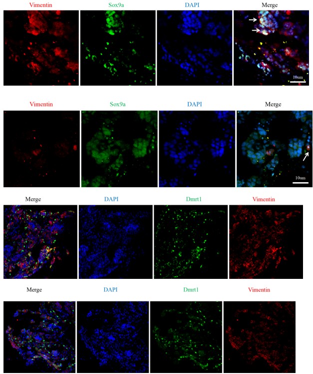
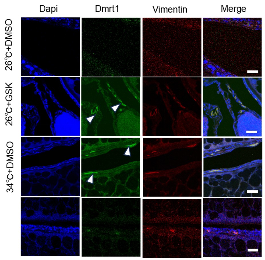
    1. eLife Assessment

      This important study investigates how the brain categorizes written words from different writing systems (e.g., alphabetic vs. non-alphabetic). The evidence supporting the authors' claims is solid and sheds light on the neural basis of language's social‑categorization function.

    2. Reviewer #1 (Public review):

      Summary:

      This study demonstrates, through a series of EEG and MEG experiments, that the human brain automatically categorizes words from alphabetic and non-alphabetic languages, and it unpacks the neural mechanisms of this process from multiple angles. The work examines not only univariate repetition-suppression (RS) effects, but also how repeating or alternating languages influences the representational similarity of words within and across language categories.

      Strengths:

      The univariate RS effects across multiple experiments lend support to some of the main conclusions.

      Comments on revised version.

      The authors have made appropriate revisions and supplements in response to the issues I raised, which has largely resolved my concerns.

    3. Reviewer #2 (Public review):

      Summary:

      This study investigates how the human brain categorizes visual words from distinct writing systems (alphabetic vs. non-alphabetic). Using a repetition suppression paradigm combined with electroencephalography and magnetoencephalography, the authors conducted nine experiments with independent participants to identify the neural network underlying language-based categorization, characterize its temporal dynamics, and test whether this process operates independently of linguistic properties such as semantic meaning and pronunciation.

      Strengths:

      The study employs a well-validated design with clear control conditions and systematically manipulates key variables including writing system, language familiarity, and native language background. The use of nine experiments with independent participant samples strengthens the reliability and replicability of the results. The work combines EEG and MEG, cross-validating findings across imaging modalities to support the reported neural effects. A combination of univariate, multivariate, and connectivity analyses is used to characterize neural responses and network interactions. Results are consistent across multiple language groups and for both familiar and unfamiliar languages, supporting the generalizability of the identified neural mechanism beyond specific languages or prior experience.

      Comments on revised version.

      Earlier versions of the manuscript framed these findings as more directly reflecting the social-categorization function of language. In the revised manuscript, the authors now more carefully distinguish language-based word categorization from broader claims regarding social categorization and explicitly acknowledge that the current experiments do not directly test social evaluation or intergroup processes. These revisions improve the conceptual precision of the work and address my major concern from the previous review.

      The additional methodological clarifications and supplementary analyses also strengthen the manuscript. Overall, I believe the revised version provides solid evidence for rapid language-based categorization of visual words across different writing systems.

    4. Author response:

      The following is the authors’ response to the original reviews.

      eLife Assessment

      This important study investigates how the brain categorizes written words from different writing systems (e.g., alphabetic vs. non-alphabetic), shedding potential light on the neural basis of language's social‑categorization function. Overall, the evidence supporting the authors' claims is solid, though some analyses and key interpretations would benefit from fuller justification.

      Thank you for handling our manuscript! We’ve modified the manuscript according to the reviewers’ comments and suggestions.

      Public Reviews:

      Reviewer #1 (Public review):

      Summary:

      This study demonstrates, through a series of EEG and MEG experiments, that the human brain automatically categorizes words from alphabetic and non-alphabetic languages, and it unpacks the neural mechanisms of this process from multiple angles. The work examines not only univariate repetition-suppression (RS) effects, but also how repeating or alternating languages influences the representational similarity of words within and across language categories.

      Strengths:

      The univariate RS effects across multiple experiments lend support to some of the main conclusions

      Weaknesses:

      I have reservations about the logic underlying the multivariate analyses, and I believe the implications of the control experiments merit fuller discussion.

      (1) Question 1: Logic of the multivariate analyses

      The original text states:

      "The processing of intra-language similarity was quantified as correlation distances between neural responses to two words of the same language, which occurred more frequently and would be inhibited in the Rep-Cond (vs. Alt-Cond) due to habituation (Fig. 1c)...".

      I argue that this passage conflates two levels. Building a representational dissimilarity matrix (RDM) is a data-analysis step; it cannot be equated with a cognitive computation. Hence, there is no sense in which this computation occurs "more frequently" in one condition. RDM construction rests on the pairwise similarity of activity patterns, so even if a task engaged no cognitive computation of representational similarity, we could still compute an RDM. Conversely, if a task factor alters the RDM, we must explain how that factor changes the underlying neural patterns, not claim that it triggers specific cognitive processing. Therefore, I neither understand what "more frequent processing" the authors refer to, nor accept their account of the multivariate results.

      The multivariate result pattern, briefly, is that distances between words, both within and across languages, are larger under the repetition condition. One plausible interpretation is that a word representation comprises two parts: language-type (alphabetic vs. non-alphabetic) and fine-grained identity features (visual shape, orthography, semantics, phonology, etc.). Repetition of language type may, via RS, reduce the weight of the first component, thereby increasing the relative contribution of fine-grained features and amplifying inter-word differences. This could explain the multivariate findings.

      Thank you for these insightful comments regarding the logic of the multivariate analyses. In the revision, we’ve elaborated the rationale underlying our experimental design. Specifically, we’ve explained why the processing of intra-language similarity is expected to occur more frequently in the repetition condition (Rep-Cond) than in the alternation condition (Alt-Cond) whereas the reverse is true for the processing of inter-language difference. Importantly, we’ve clarified that the processing of intra-language similarity was assessed rather than defined by conducting the multivariate analyses. The multivariate analyses were conducted to assess correlation distances between neural responses to pairs of words, either within the same language or across different languages. We explained what smaller intra-language correlation distances and larger inter-language correlation distances mean for language-base categorization of words (see Page 7-8).

      We appreciate the alternative account of the observed neural repetition suppression (RS) effects in terms of language-type versus fine-grained identity (visual shape, orthography, semantics, phonology, etc.) feature processing. We included a paragraph in the revised Discussion to discuss how possible the early neural RS effect can be attributed to the processing of the fine-grained identity features of visual words. This discussion allowed us to clarify that the early neural RS effects related to visual words of familiar and unfamiliar languages highlight the early spontaneous language-based categorization as a unique process of visual words of alphabetic and non-alphabetic languages. However, our results do not exclude the possibility that the processing of the linguistic properties of visual words may contribute to the long-latency RS effect (see Page 37-38).

      Page 7-8

      “The processing of intra-language similarity occurs when two words of the same language are perceived repeatedly with short interstimulus intervals. Because words of the same language were repeatedly presented in the Rep-Cond and words of two different languages were displayed in the Alt-Cond, the processing of intra-language similarity occurred more frequently and would be inhibited in the Rep-Cond (vs. Alt-Cond) due to habituation (Fig. 1c). By contrast, the processing of inter-language difference takes place when two words of different languages are perceived with short interstimulus intervals. Since words of different languages appeared more frequently in the Alt-Cond (vs. Rep-Cond), we would expect RS of the processing of inter-language difference in the Alt-Cond (vs. Rep-Cond). The neural processing of intra-language similarity was quantified as correlation distances between neural responses to two words of the same language whereas the neural processing of inter-language difference was assessed as correlation distances between neural responses to two words of two different languages. The correlation distances from the multivariate analyses were further employed to assess how words of one language are clustered and how far words of two languages are separated in a two-dimensional (2D) space during language-based word categorization. Enhanced language-based word categorization is associated with smaller intra-language correlation distances, which reflect more densely clustered words of the same language, and larger inter-language correlation distances, which manifest further separated words of two different languages.”

      Page 37-38

      “How possible are the early neural RS effects within 200 ms after word onset observed in our study related to the processing of low-level perceptual features or high-level linguistic (e.g., orthography, semantics, phonology) properties of visual words? Our analyses of the ERPs to scrambled Chinese and English words in Experiment 2 did not show significant RS effect. Because only low-level visual features were preserved in the scrambled words, the ERP results provided no evidence that the early RS effects on the neural response to words can be attributed to habituation of perception of the low-level perceptual features. Furthermore, we found that the RS effects on the neural response to radicals and letters in Experiment 3 took place in a delayed time window and exhibited different scalp distributions (i.e., over the central region for radicals and occipital regions for letters) compared with the neural RS effects related to words. Thus the early RS effects on the neural response to words cannot be interpreted as habituation of perception of the middle-level units of Chinese and English words (i.e., radicals and letters) either. In addition, the early neural RS effects were similarly observed for both familiar (i.e., Chinese and English) and unfamiliar (i.e., Korean and Italian) languages and occurred earlier than the time window in which the processing of the linguistic properties of visual words takes place (Marinkovic et al., 2003; Hodgson et al., 2021; Zhu et al., 2022). Therefore, the early neural RS effects identified in our work were unlikely to be associated with the processing of the linguistic (e.g., orthography, semantics, phonology) properties of visual words since these properties of unfamiliar languages were unknown to the participants. Taken together, our findings of the early neural RS effects highlight an early word-level representation of alphabetic vs. non-alphabetic languages which distinguishes words from letters/radicals but is similar for familiar or unfamiliar languages. Our results, however, do not exclude the possibility that the processing of the linguistic properties of visual words may contribute to the long-latency RS effect around 300 ms after word onset. Further processing of the linguistic properties of visual words of familiar languages may follow the early language-based categorization of visual words, though this should be tested in future research.”

      (2) Question 2:

      For unlearned languages, people cannot distinguish lexical from sub-lexical levels. What, then, determines (i) the RS-effect difference between letters and radicals in familiar languages and words in unlearned ones, and (ii) the similarity of repetition effects between words in unlearned and familiar languages? An explicit account is needed.

      Thank you for this suggestion. In the revised manuscript, we’ve included a dedicated paragraph addressing these two issues. Specifically, we’ve provided a more precise account of the differences in repetition suppression (RS) effects between words and letters/radicals in familiar languages, as well as the similar RS effects observed for unlearned and familiar languages. We believe that our findings of the early neural RS effects highlight an early word-level representation of alphabetic vs. non-alphabetic languages which distinguishes words from letters/radicals but is similar for familiar or unfamiliar languages (see Page 37-38).

      Page 37-38

      “How possible are the early neural RS effects within 200 ms after word onset observed in our study related to the processing of low-level perceptual features or high-level linguistic (e.g., orthography, semantics, phonology) properties of visual words? Our analyses of the ERPs to scrambled Chinese and English words in Experiment 2 did not show significant RS effect. Because only low-level visual features were preserved in the scrambled words, the ERP results provided no evidence that the early RS effects on the neural response to words can be attributed to habituation of perception of the low-level perceptual features. Furthermore, we found that the RS effects on the neural response to radicals and letters in Experiment 3 took place in a delayed time window and exhibited different scalp distributions (i.e., over the central region for radicals and occipital regions for letters) compared with the neural RS effects related to words. Thus the early RS effects on the neural response to words cannot be interpreted as habituation of perception of the middle-level units of Chinese and English words (i.e., radicals and letters) either. In addition, the early neural RS effects were similarly observed for both familiar (i.e., Chinese and English) and unfamiliar (i.e., Korean and Italian) languages and occurred earlier than the time window in which the processing of the linguistic properties of visual words takes place (Marinkovic et al., 2003; Hodgson et al., 2021; Zhu et al., 2022). Therefore, the early neural RS effects identified in our work were unlikely to be associated with the processing of the linguistic (e.g., orthography, semantics, phonology) properties of visual words since these properties of unfamiliar languages were unknown to the participants. Taken together, our findings of the early neural RS effects highlight an early word-level representation of alphabetic vs. non-alphabetic languages which distinguishes words from letters/radicals but is similar for familiar or unfamiliar languages. Our results, however, do not exclude the possibility that the processing of the linguistic properties of visual words may contribute to the long-latency RS effect around 300 ms after word onset. Further processing of the linguistic properties of visual words of familiar languages may follow the early language-based categorization of visual words, though this should be tested in future research.”

      Reviewer #2 (Public review):

      Summary:

      This study investigates how the human brain categorizes visual words from distinct writing systems (alphabetic vs. non-alphabetic) as a neural basis for the social-categorization function of language. Using a repetition suppression paradigm combined with electroencephalography and magnetoencephalography, the authors conducted nine experiments with independent participants to identify the neural network underlying language-based categorization, characterize its temporal dynamics, and test whether this process operates independently of linguistic properties such as semantic meaning and pronunciation.

      Strengths:

      (1) The study employs a well-validated design with clear control conditions and systematically manipulates key variables, including writing system, language familiarity, and native language background. The use of nine experiments with independent participant samples strengthens the reliability and replicability of the results.

      (2) The work combines EEG and MEG, cross-validating findings across imaging modalities to support the reported neural effects. A combination of univariate, multivariate, and connectivity analyses is used to characterize neural responses and network interactions.

      (3) Results are consistent across multiple language groups and for both familiar and unfamiliar languages, supporting the generalizability of the identified neural mechanism beyond specific languages or prior experience.

      Weaknesses:

      The authors provide compelling evidence that the identified neural network supports the categorization of words by language, including computations of intra-language similarity and inter-language difference. However, the conceptual framing of this finding as directly reflecting the social-categorization function of language may be premature. While the task captures spontaneous language categorization, it does not involve social evaluation or intergroup processes. The connection to social categorization is inferred from prior literature rather than demonstrated within the current experimental design. Clarifying this distinction would strengthen the conceptual precision of the manuscript.

      Thank you for this important comment. In the revised Introduction and Discussion, we’ve clarified several related issues. First, prior research suggests that language can serve as a socially relevant category cue. Second, these findings imply that rapid categorization of words by language may occur in the human brain. Third, although our results identify a neural network supporting such rapid language-based categorization of visual words, they do not directly test how this process relates to social categorization of people (see Page 3-4; Page 39). Highlighting these points help delineate the scope of our findings and point to important directions for future research.

      Page 3-4

      “The social-categorization function of language revealed in these behavioral studies implicates that rapid categorization of words of different languages may occur in the human brain. Furthermore, the findings of infant studies (e. g., Liberman et al., 2017b) suggest that the neural process involved in categorization of words of different languages may develop even prior to the processing of linguistic properties (e.g. semantic meanings) of words. Nevertheless, up to date, there has been little neuroimaging research examining the neural mechanisms underlying automatic and fast categorization of words of different languages.”

      Page 39

      “Finally, it should be noted that the current work was initiated by the previous behavioral findings which suggest that language can serve as a socially relevant category cue but focused on the neural mechanisms underlying rapid language-based categorization of visual words. Although the previous findings suggest that the language-based categorization of visual words provides a cognitive basis of social categorization of people, our work did not directly test whether and how the neural processes involved in the language-based categorization of visual words are linked to social evaluation or intergroup processes which are critical for social categorization of people. To clarify this issue should promote deep comprehension of the neural mechanisms underlying the social-categorization function of language but is beyond the scope of the current study. Future research should investigate the connection between language-based categorization of words and social categorization based on other social cues (e.g., faces), which is pivotal to understanding of social interactions in real-world situations.”

      Recommendations for the authors:

      Reviewer #2 (Recommendations for the authors):

      (1) Revise the conceptual framing to clarify the relationship between the experimental results and the proposed social-categorization function of language. If the authors wish to retain the emphasis on social categorization in the title or discussion, they should explicitly explain how the observed neural mechanisms of language-based word categorization link to social evaluation, intergroup processes, or real-world social categorization. This clarification would strengthen the conceptual coherence and justify the use of social categorization within the current study's scope.

      Thank you for this and the following suggestions. In the revised Introduction and Discussion, we’ve clarified the following point: First, the findings of prior behavioral studies suggest a social-categorization function of language. Second, based on these behavioral findings, we predicted automatic and fast categorization of words by language. Our study tested this prediction using neuroimaging and investigated the neural mechanisms of language-type-based categorization of visual words. This is the main goal of our work. Third, to examine how the observed neural mechanisms of language-based word categorization link to social evaluation, intergroup processes, or real-world social categorization is important but beyond the scope of the current work. However, this is a very important question. Future research should test the connection between the neurocognitive processes involved in social categorization of people and the neural categorization of visual words by language revealed in our study. Consistently, the title of our paper “Neural categorization of visual words of alphabetic and non-alphabetic languages” and Discussion focus on contributions of our findings to understanding of the neural categorization of visual words by language rather than its connection to social categorization of people. Above all, we’ve clarified in the revision that our study was initiated by the findings of social function of language but was limited to the neural processing of visual words (see Page 3-4; Page 39). Thanks again for this comment.

      Page 3-4

      “The social-categorization function of language revealed in these behavioral studies implicates that rapid categorization of words of different languages may occur in the human brain. Furthermore, the findings of infant studies (e. g., Liberman et al., 2017b) suggest that the neural process involved in categorization of words of different languages may develop even prior to the processing of linguistic properties (e.g. semantic meanings) of words. Nevertheless, up to date, there has been little neuroimaging research examining the neural mechanisms underlying automatic and fast categorization of words of different languages.”

      Page 39

      “Finally, it should be noted that the current work was initiated by the previous behavioral findings which suggest that language can serve as a socially relevant category cue but focused on the neural mechanisms underlying rapid language-based categorization of visual words. Although the previous findings suggest that the language-based categorization of visual words provides a cognitive basis of social categorization of people, our work did not directly test whether and how the neural processes involved in the language-based categorization of visual words are linked to social evaluation or intergroup processes which are critical for social categorization of people. To clarify this issue should promote deep comprehension of the neural mechanisms underlying the social-categorization function of language but is beyond the scope of the current study. Future research should investigate the connection between language-based categorization of words and social categorization based on other social cues (e.g., faces), which is pivotal to understanding of social interactions in real-world situations.”

      (2) Clarify the consistency between the reported model order (5 ms lag) and the sampling rate after downsampling (250 Hz, corresponding to 4 ms per time point). If a discrepancy exists, clearly explain how the time-series data were processed.

      We clarified in the revision (see Page 53) that “because down-sampling was not applied to the GCA analyses, a 5-ms lag was used for prediction of the neural activity in one brain region using the neural activity in another brain region”.

      (3) For the representational similarity analysis (RSA), report reliability measures for the representational dissimilarity matrices (e.g., split-half reliability) to verify that the observed effects are stable given the number of trials per condition.

      Following this suggestion, we’ve conducted split-half reliability analyses and reported the results in the revised supplementary materials. The reliability analyses are also mentioned in the revised Discussion (see Page 40).

      Page 40

      “In conclusion, our EEG and MEG results revealed robust RS effects in the early neural responses to visual words of the same language. The reliability of these RS effects was confirmed across words of different familiar and unfamiliar languages, in samples of speakers with different native languages, and through split-half reliability analyses (see Supplementary Materials, Fig. S19). These effects were supported by the bilateral neural networks whose activity reflected computations of correlation distances between word pairs, capturing both intra-language similarity and inter-language differences during the categorization of visual words in alphabetic and non-alphabetic languages. Together, these findings advance our understanding of spontaneous, language-based neural categorization of visual words as a key basis of the social-categorization function of language.”

      (4) Provide complete statistical information for all significant results reported in the supplementary materials, including relevant test statistics (e.g., t-values, cluster p-values) in figure legends or a supplementary results table to improve transparency.

      Complete statistical information has been provided in the revised supplementary materials (see Tables S4 and S5).

      (5) Streamline the presentation of the nine experiments in the main text to emphasize the core conceptual and methodological logic, potentially using a schematic overview or flowchart to improve readability.

      As suggested, we’ve included an overview of the nine experiments in the revised Introduction. This overview helps understanding of the core conceptual and methodological issues in our work (see Page 6).

      Page 6

      “In nine experiments we recorded EEG/MEG signals from Chinese, English, and German speakers when viewing words of an alphabetic language and a non-alphabetic language (English and Chinese words, or Italian and Korean words) or of two alphabetic languages (English and German) in the Rep-Cond and Alt-Cond. We recorded EEG signals from Chinese participants to examine temporal neural dynamics of spontaneous language-based word categorization in Experiment 1. The similar paradigm was employed in Experiments 2 and 3 to investigate whether perceptual features or radical/letters of words are sufficient to generate spontaneous language-based categorization of visual words. The results in Experiment 1 were replicated in native English and German speakers in Experiments 4 and 5, respectively. Neural dynamics of categorization of words of two unlearned languages were further investigated in Chinese participants in Experiment 6. Finally, the neural networks supporting the spontaneous categorization of words of two learned or unlearned languages were localized using MEG in Chinese and English speakers in Experiments 7-9, respectively.”

      (6) Strengthen the transition between the discussion of the social-categorization function of language and the neural mechanisms of visual word categorization in the introduction.

      Following this suggestion, we’ve modified the Introduction to strengthen the transition between the discussion of the social-categorization function of language and research on neural mechanisms of visual word categorization (see Page 3-4).

      Page 3-4

      “The social-categorization function of language revealed in these behavioral studies implicates that rapid categorization of words of different languages may occur in the human brain. Furthermore, the findings of infant studies (e. g., Liberman et al., 2017b) suggest that the neural process involved in categorization of words of different languages may develop even prior to the processing of linguistic properties (e.g. semantic meanings) of words. Nevertheless, up to date, there has been little neuroimaging research examining the neural mechanisms underlying automatic and fast categorization of words of different languages.”

      (7) Briefly define the repetition suppression (RS) paradigm when first mentioned (i.e., reduced neural response to repeated stimuli from the same category, reflecting categorical processing) to improve accessibility for non-specialist readers.

      The RS paradigm is now defined in Introduction when being mentioned for the first time in the manuscript (see Page 5-6).

      Page 5-6

      “The present study investigated neural dynamics of categorization of visual words of two different (an alphabetic versus a non-alphabetic, or two different alphabetic) languages by combining EEG/MEG with a repetition suppression (RS) paradigm adopted from previous studies of social categorization of faces (Zhang et al., 2023b; Zhou et al., 2020). RS refers to the attenuation in neural responses to a repeated occurrence of stimuli that engage common neuronal populations or processes due to habituation (Grill-Spector et al., 2006). The RS paradigm consisted of an alternating condition (Alt-Cond), in which visual words of two different languages were presented alternately, and a repetition condition (Rep-Cond), in which words of one language were presented repeatedly (Fig. 1a). Neural responses to stimuli of the same category were attenuated in the Rep-Cond compared to Alt-Cond due to habituation and this RS effect disentangles the neural activities underlying categorization of faces and body silhouettes of a specific social group.”

      (8) Report detailed participant demographic information, including exact age range/mean age and gender ratio for each experiment, to meet standard reporting practices in neuroscience.

      We’ve modified Table S1 to include the information about exact age range/mean age and gender ratio in each experiment.

      (9) Correct minor typographical and grammatical errors, including These finding (line 59) and Chinse (line 223).

      These and other grammatical errors have been corrected in the revision.

    1. eLife Assessment

      This valuable study compares auditory cortex responses to sounds and cochlear implant stimulation measured with surface electrode grids in rats. Beyond the reduced frequency resolution of cochlear implants observed previously, this study suggests key discrepancies between neuronal representations of cochlear stimulations and natural sounds. The evidence for this result is solid but could be strengthened with a clarification of the methodology and an adaptation of the claim to the actual precision of the measurements. This study is of interest to researchers in the auditory neuroscience field and clinicians implementing treatments with cochlear implants.

    2. Reviewer #1 (Public review):

      Summary

      This manuscript addresses an important question in auditory neuroscience and neuroprosthetics: whether cortical responses to cochlear implant stimulation resemble those evoked by natural acoustic stimulation, or whether electrical stimulation engages a distinct cortical representation. The authors use high-density intracranial EEG recordings in rats to compare responses to pure tones in normal-hearing animals with responses to single-channel cochlear implant stimulation in deafened animals. They combine analyses of event-related potentials, high-gamma activity, trial-by-trial variability, PCA/TCA-based dimensionality reduction, and decoder-based measures of stimulus information.

      Strengths

      A major strength of the study is the question it addresses. Understanding how electrical cochlear stimulation is represented centrally is highly relevant for cochlear implant design, fitting strategies, and rehabilitation. The comparison between acoustic and electrical stimulation, including within-animal comparisons in a subset of cases, is valuable because it directly addresses whether implant-evoked activity can be interpreted within the framework of normal acoustic tonotopy.

      The methodological approach is also a strength. Dense cortical surface recordings provide simultaneous access to spatial and temporal features of auditory cortical responses. The combination of PCA, TCA, and decoder analyses gives complementary views of the data, and the information-transfer analysis provides an interesting way to ask whether representations learned from acoustic stimulation generalize to electrical stimulation.

      Weaknesses:

      The main weakness is that the evidence for spatial organization remains difficult to interpret. In Figure 2, the authors argue that both tone-evoked and cochlear implant-evoked responses are spatially organized, but the slope analyses are not significant for the cochlear implant condition. The revised vector-strength analysis supports the presence of non-random spatial structure, but this is not the same as demonstrating a clear graded cochleotopic organization. The manuscript would be strongest if it consistently distinguished between non-random spatial structure, coarse topography, and true graded tonotopy or cochleotopy.

      A related issue is that some figure titles and interpretive statements still appear stronger than the data justify. For example, the TCA results in Figure 7 are described as revealing topographically organized latent spatial factors, but the statistical support appears strongest for normal-hearing high-gamma responses, with weaker or non-significant results in other conditions. These data remain interesting, but they would be better framed as evidence for weak or coarse spatial structure rather than robust topographic organization across all modalities.

      The decoder analyses are improved, especially with the added tone-to-tone control. This control supports the conclusion that poor acoustic-to-CI transfer is not simply a failure of the TCA/LDA pipeline. However, the analysis remains model-dependent, and the absolute information transfer values are low. It would be helpful either to include an analogous analysis using raw ERP/high-gamma features or to explain more explicitly why the TCA-based approach is the appropriate primary test. The data support poor generalization between acoustic and implant-evoked cortical responses, but claims about perceptual qualities should remain speculative because perception is not directly measured in these experiments.

      Finally, although methodological reporting is much improved, some verification remains indirect. The authors provide useful implantation criteria and cite prior validation of their deafening approach, but the manuscript would be clearer if it explicitly distinguished between validation performed in the present animals and validation based on previous cohorts. This distinction is important because surgical variability, implantation efficacy, and deafening completeness can influence the interpretation of cochlear implant experiments.

      Comments on revised version.

      The revised manuscript is considerably improved. The authors have clarified several methodological details, added a statistical framework that better accommodates both paired and unpaired animals, provided a clearer account of animal cohorts, added peripheral ECAP/forward-masking data to support the cochlear specificity of implant stimulation, and included a useful positive control for the cross-modal decoder analysis. These additions make the manuscript stronger and help readers interpret the main findings more confidently.

      The results support the conclusion that acoustic and cochlear implant stimulation evoke cortical responses with different properties. In particular, acoustic responses support better single-trial stimulus decoding than cochlear implant responses, and decoders trained on acoustic responses transfer poorly to implant-evoked responses. The evidence for spatial organization is more nuanced. The cochlear implant condition shows evidence of non-random spatial structure, but not a clear graded cochleotopic map. The normal-hearing condition is also less visually clear than might be expected from prior tonotopy studies, although the added analyses and comparisons to previous work help contextualize this result. Overall, the study makes a valuable contribution, provided that the claims about spatial organization and perceptual interpretation remain appropriately cautious.

      The revision addresses several important concerns from the original version. The use of mixed-effects models better matches the partially paired experimental design. The expanded Methods improve reproducibility. The new cohort schematic helps clarify which animals contributed to behavioral and neural datasets. The ECAP forward-masking measurements add useful peripheral validation, and the within-modality decoder control strengthens the interpretation of the poor cross-modal transfer result. Together, these changes substantially improve the manuscript.

      The work is likely to be of interest to auditory neuroscientists, cochlear implant researchers, and neuroengineers. Even where some conclusions require cautious wording, the dataset and analytical framework may be useful for future studies aiming to relate cortical responses to implant programming, perceptual learning, or closed-loop neuroprosthetic approaches.

      Overall, the revised manuscript is stronger and addresses an important problem with useful methods and analyses. The results most convincingly show that acoustic responses support better single-trial decoding than acute cochlear implant responses, and that acoustic-trained decoders generalize poorly to implant-evoked activity. The evidence for robust spatial organization, especially in the cochlear implant condition, is more limited and should be presented with appropriate caution.

    3. Reviewer #2 (Public review):

      Summary:

      This article reports measurements of iEEG signals on the rat auditory cortex during cochlear implant or sound stimulation in separate groups of rats. The observations indicate some spatial organization of cochlear implant stimuli, but that is very different from cochlear implants.

      Strengths:

      The study includes interesting analyses of the sound and cochlear implant representation structure based on decoders.

      Weaknesses:

      The observation that responses to cochlear implant stimulation (stimulation) is spatially organized is not new (e.g. Adenis et al. 2024)

      The claim that spatial and temporal dimensions contribute information about the sound is also not new there is a large literature on this topic.

      The analyses supporting the claim that there is a mismatch between cochlear implant and sound representation are still unclear, particularly in Fig. 8.

    4. Reviewer #3 (Public review):

      Summary:

      Through micro-electroencephalography, Hight and colleagues studied how the auditory cortex in its ensemble respond to cochlear implant stimulation compared to the classic pure tones. Taking advantage of a double implanted rat model (Micro-ECoG and Cochlear Implant), they tracked and analyzed changes happening in the temporal and spatial aspects of the cortical evoked responses in both normal hearing and cochlear-implanted animals. After establishing that single trial responses were sufficient to encode the stimuli properties, the authors then explored several decoder architectures to study the cortex ability to encode each stimuli modality in a similar or different manner. They conclude that a) intracranial EEG evoked responses can be accurately recorded and did not differed between normal hearing and cochlear-implanted rats; b) Although coarsely spatially organized, CI-evoked responses had higher trial-by-trial variability than pure tones; c) Stimulus identity is independently represented by temporal and spatial aspect of cortical representations and can be accurately decoded by various means from single trials; d) and that Pure tones trained decoder can't decode CI-stimulus identity accurately.

      Strength:

      The model combining micro-eCoG and cochlear implantation and the methodology to extract both the Event Related Potentials (ERPs) and High-Gammas (HGs) is very well designed and appropriately analyzed. Likewise, the PCA-LDA and TCA-LDA are powerful tools that take full advantage of the information provided by the cortical ensembles.

      The overall structure of the paper, with a paced and exhaustive progress through each step and evolution of the decoder is very appreciable and easy to follow. The exploration of single trial encoding and stimulus identity through temporal and spatial domains is providing new avenues to characterize the cortical responses CI stimulations and their central representation. The fact that single trials suffice to decode the stimulus identity regardless of their modality is of great interest and noteworthy. Although the authors confirm that iEEG remains difficult to transpose in clinic, the insights provided by the study confirm the potential benefit of using central decoders to help in clinic settings.

      Weakness:

      The conclusion of the paper, especially the concept of distinct cortical encoding for each modality, is unfortunately partially supported by the results as the authors ignored fundamental limitations of CI related stimulation.

      First, the authors stimulated in a Monopolar mode which, albeit being clinically relevant, notoriously generates a high current spread in rodent models. Comparing the averaged BF maps for iEEG (Fig-2A, C), BFs ranged from 4 to 16kHz with a predominance of 4kHz BFs. The lack of BFs at higher frequencies might reveal a potential location mismatch between the frequency range sampled at the level of the cortex (low to medium frequencies) and the frequency range covered by the CI inserted mostly in the first turn-and-a-half of the cochlea (high to medium frequencies). Looking at Fig-2F (and to some extend 2A) most of CI electrodes elicited responses around the 4kHz regions and averaged maps show a predominance of CI-3-4 across cortex (Fig-2C, H and Sup Fig. 3) from areas with 4kHz BF to areas with 16kHz BF. It is doubtful that CI-3-4 are located near the 4kHz region based on Müller's work (1991) on the frequency representation in the rat cochlea. Moreover, Supplemental figure 3 shows that only a couple of CI electrodes are predominately represented at the level of the cortex. Thus, it seems possible that current spread ended stimulating indistinctly higher turns of the cochlea or even the modiolus in a non-specific manner, greatly reducing (or smearing) the place-coding/frequency resolution of each electrode, which in turn could explain the coarse topographic (or coarsely tonotopic according to the manuscript) organization of the cortical responses.

      Second, although the authors acknowledge that post-lingual CI users always have an adaptation period, their conclusion is based on measurements that are relatively "early" in the CI-use timeline so to speak since iEEG were collected a) acutely right after mono-aural implantation and stimulation, b) under anesthesia, c) using unmodulated pulse train fixed at 900pps regardless of the electrode used and thus lacking any temporal information shifts in relationship to electrode cochleotopic placement. Basically, all CI electrodes had the same rate whereas you would expect basal CI electrodes to be amplitude modulated at higher frequencies than apical electrodes.

      As much as the reviewer likes the overall approach with the use of PCA-LDA and TCA, and agrees that information transfer seems inexistant at time of measurement, authors should be more careful in their strong conclusion that two distinct encoding exist. The non-overlapping between sound and electric stimulation representations might exist only transiently and this should be acknowledged a bit more in the discussion. Without repetition of iEEG measurement at later period with chronic use of the CI, it is not possible to definitively claim that two distinct, non-overlapping coding co-exist at all times.

      Nevertheless, the reviewer wants to reiterate that the study proposed by Hight et al. is well constructed, relevant to the field and that the overall proposal of improving patient performances and help their adaptation in the first months of CI use by studying central responses should be pursued as it might help establish new guidelines or create new clinical tools.

    5. Author response:

      The following is the authors’ response to the original reviews

      Summary of revision for all referees:

      We thank referees for their constructive comments. To address their concerns, we now performed additional statistical analyses integrating both paired and unpaired data, performed positive controls for comparisons between NH- and CI- evoked iEEG measurements, developed tools for measuring and collected new experimental data on forward masking ECAP measurements in CI implanted rats (N=3), and reworked both manuscript text and figures to improve clarity. These most significant changes are summarized here, and a complete list of responses to reviewers and corresponding changes will follow.

      Summary of major changes to revised manuscript:

      (1) Statistical treatment of paired vs unpaired recordings using mixed-effects models (updates to all manuscript figures that compare NH vs CI); this largely confirmed the results reported in our original submission.

      (2) New analysis, controlling for information-theoretic cross-modality comparison (i.e., training with tone- and testing with cochlear implant-evoked iEEG measures, Fig. 8).

      (3) Clarification of methods (Supplemental Fig. 2 & manuscript text)

      (4) Additional experiments testing peripheral tuning of our 8-channel CI rodent model via forward masking ECAP measures across 3 animals (N=3, Supplemental Fig. 1)

      (5) Detailed response addressing robustness of tonotopy in NH and CI animals

      Public Reviews:

      Reviewer #1 (Public Review):

      Strengths:

      The study poses a timely, clinically relevant question with clear implications for CI strategy. The analytical toolkit is appropriate: µECoG captures mesoscale patterns; TCA offers a transparent separation of spatial and temporal structure; and mutual-information decoding provides an interpretable measure of single-trial discriminability. Within-subject recordings in a subset of animals, in principle, help isolate modality effects from inter-animal variability. Where analyses are most direct, the acoustic condition yields higher single-trial decoding accuracy, which is a meaningful and clearly presented result.

      We appreciate the comments on the strengths of our analytic approaches.

      Weaknesses:

      Parts of the statistical treatment do not match the data structure: some comparisons mix paired and unpaired animals but are analysed as fully paired, raising concerns about misestimated uncertainty.

      Please see our response to specific comment #2 above. In short, we agree with this critique of our original analyses, and in our revised manuscript we re-analyzed all NH vs. CI comparisons using linear mixed effects models that incorporate both paired and unpaired observations within a single framework. This allows us to include all animals, account for within-animal dependence for paired experiments (normal hearing and cochlear implant data from the same animal when available), and to align the statistical tests with the data shown in the figures. In almost every case, the mixed effects models confirm our original conclusions. Two comparisons that were previously nonsignificant now reach criterion for statistical significance (Fig. 2E, p=0.048 and Fig. 6F, p=0.027). We updated the manuscript to report these values and to clarify the use of mixed effects modeling in the methods under the section titled, “Linear mixed effects modeling.”

      Methodological reporting is incomplete in places; essential parameters for both acoustic and electrical stimulation, as well as objective verification of implantation and deafening, are not described with sufficient detail to support confident interpretation or replication.

      Please see our response to comment #5 below. We have revised our manuscript to now include this information in the methods.

      Figure-level clarity also undermines the message. In Figure 2, non-significant slopes for CI, repeated identification of a single "best channel," mismatched axes, and unclear distinctions between example and averaged panels make the assertion of spatial organisation unconvincing; importantly, the normal-hearing panels also do not display tonotopy as clearly as expected, which weakens the key contrast the paper seeks to establish.

      This is an important point, thanks- please see responses to comment #1 above. We note that conventional tonotopic maps in auditory cortex are characteristic frequency maps, i.e., maps of topographic organization for responses to lowest-threshold stimuli (often presented around 20-50 dB SPL). Our maps were constructed from stimuli presented at 70 dB SPL, thus blunting crisp tonotopy to some degree. Furthermore, we quantified spatial organization using a previously published method from the Polley lab (Romero & Hight et al. 2020), in which local tonotopic gradient vectors (magnitude and direction) were computed from GCaMP responses at each pixel and projected onto a unit circle. Mean vector strength across all pixels was then compared to a shuffled distribution as a measure of tonotopic organization. We applied the same procedure to our iEEG best-frequency and best-channel maps. Both map types yielded mean vector strengths that were substantially larger than those derived from shuffled maps (p < 10<sup>-10</sup>), indicating that our maps have a consistent tonotopic (for BFs) or cochleotopic (for CI channels) organization that is highly unlikely to arise by chance. This is now included in our revised manuscript.

      Finally, the decoding claims would be strengthened by simple internal controls, such as within modality train/test splits and decoding on raw ERP/high-gamma features to demonstrate that poor cross-modal transfer reflects genuine differences in the underlying responses rather than limitations of the modelling pipeline.

      Please see our response to comment #12 below. In short, we have now included this analysis in revised Figure 8.

      Reviewer #2 (Public Review):

      Strengths:

      The study includes interesting analyses of the sound and cochlear implant representation structure based on decoders.

      We appreciate the comment on how interesting our analyses are, thanks!

      Weaknesses:

      The observation that responses to cochlear implant stimulation (stimulation) are spatially organized is not new (e.g., Adenis et al. 2024).

      We agree that it is not particularly novel to report that there is spatial organization to cochlear implant stimulation. However, we believe that our direct comparisons (when possible, within animal) between normal-hearing and cochlear implant modality maps is unusual in the literature, including asking how decoders based on one set of responses might apply to responses evoked from the other modality. Adenis et al. (2024) is a fantastic study of pulse shape and monopolar vs bipolar stimulation modes with a 6-channel implant in guinea pig, but as far as we can tell this study does also not compare normal hearing maps prior to deafening and implantation to the cochlear implant maps in the same animals.

      The claim that spatial and temporal dimensions contribute information about the sound is also not new; there is a large literature on this topic. Moreover, the results shown here are extremely weak. They show similar levels of information in the spatial and temporal dimensions, and no synergy between the two dimensions. This is however, likely the consequence of high measurement noise leading to poor accuracy in the information estimates, as the authors state.

      Good point, please see our response to comment #1 below.

      The main claim of the study - the mismatch between cochlear implant and sound representation - is not supported. The responses to each modality are measured in different animals. The authors do not show that they actually can compare representations across animals (e.g., for the same sounds). Without this positive control, there is no reason to think that it is possible to decode from one animal with a decoder trained on another, and the negative result shown by the authors is therefore not surprising.

      Good point, thanks- please see our response to comment #2 below, where we describe this new control we have added.

      Reviewer #3 (Public Review):

      Strengths:

      The model combining micro-eCoG and cochlear implantation and the methodology to extract both the Event Related Potentials (ERPs) and High-Gammas (HGs) is very well designed and appropriately analyzed. Likewise, the PCA-LDA and TCA-LDA are powerful tools that take full advantage of the information provided by the cortical ensembles. The overall structure of the paper, with a paced and exhaustive progress through each step and evolution of the decoder, is very appreciable and easy to follow. The exploration of single-trial encoding and stimulus identity through temporal and spatial domains is providing new avenues to characterize the cortical responses to CI stimulations and their central representation. The fact that single trials suffice to decode the stimulus identity regardless of their modality is of great interest and noteworthy. Although the authors confirm that iEEG remains difficult to transpose in the clinic, the insights provided by the study confirm the potential benefit of using central decoders to help in clinic settings… the reviewer wants to reiterate that the study proposed by Hight et al. is well constructed, relevant to the field, and that the overall proposal of improving patient performances and helping their adaptation in the first months of CI use by studying central responses should be pursued as it might help establish new guidelines or create new clinical tools.

      We thank the Reviewer for the positive comments about the thoroughness of our analyses and clear organization of our manuscript.

      Weaknesses:

      The conclusion of the paper, especially the concept of distinct cortical encoding for each modality, is unfortunately partially supported by the results, as the authors did not adequately consider fundamental limitations of CI-related stimulation. First, the reviewer assumed that the authors stimulated in a Monopolar mode, which, albeit being clinically relevant, notoriously generates a high current spread in rodent models.

      Thanks, this is an important potential concern. Please see our response to comment #5 of Referee 1 and responses to comment #3 below. We agree that monopolar stimulation would be expected to be less spatially specific than bipolar or multipolar modes. However, we chose monopolar stimulation because it is the main clinical configuration in human CI users and therefore most relevant for translational purposes. For our revised manuscript, we made new ECAP measurements of peripheral (spatial and temporal) tuning via a forward masking paradigm and demonstrate that monopolar is effectively tuned (Supplemental Fig. 2). Together with additional single-animal maps in Supplementary Figure 3, together with our vector-strength analysis (Response Fig. 2), demonstrate that even under acute monopolar stimulation we observe structured cochleotopic organization in cortex, rather than the extremely low-pass patterns one might expect if monopolar spread was a major contaminant.

      Second, comparing the averaged BF maps for iEEG (Figure 2A, C), BFs ranged from 4 to 16kHz with a predominance of 4kHz BFs. The lack of BFs at higher frequencies hints at a potential location mismatch between the frequency range sampled at the level of the cortex (low to medium frequencies) and the frequency range covered by the CI inserted mostly in the first turn-and-a-half of the cochlea (high to medium frequencies). Looking at Figure 2F (and to some extent 2A), most of the CI electrodes elicited responses around the 4kHz regions, and averaged maps show a predominance of CI-3-4 across the cortex (Figure 2C, H) from areas with 4kHz BF to areas with 16kHz BF. It is doubtful that CI-3-4 are located near the 4kHz region based on Müller's work (1991) on the frequency representation in the rat cochlea.

      Please see our responses to comment #3 below.

      Taken together with the Pearsons correlations being flat, the decoder examples showing a strong ability to identify CI-4 and 3 and the Fig-8D, E presenting a strong prediction of 4kHz and 8kHz for all the CI electrodes when using a pure tone trained decoder, it is possible that current spread ended stimulating indistinctly higher turns of the cochlea or even the modiolus in a non-specific manner, greatly reducing (or smearing) the place-coding/frequency resolution of each electrode, which in turn could explain the coarse topographic (or coarsely tonotopic according to the manuscript) organization of the cortical responses. Thus, the conclusion that there are distinct encodings for each modality is biased, as it might not account for monopolar smearing. To that end, and since it is the study's main message and title, it would have benefited from having a subgroup of animals using bipolar stimulations (or any focused strategy since they provide reduced current spread) to compare the spatial organization of iEEG responses and the performances of the different decoders to dismiss current spread and strengthen their conclusion.

      Please see our responses to comment #4 below as well as our responses related to monopolar vs bipolar stimulation. We agree that for future studies, it will be important to do a heads-on comparison of the differences between bipolar and monopolar stimulation depending on electrode location and stimulation intensity.

      Recommendations for the authors:

      Reviewer #1 (Recommendations for the authors):

      We thank the reviewer for commenting on the strengths of our manuscript, including appreciating the power and timeliness of our approach.

      (1a) Figure 2 does not convincingly support the claim that "tone-evoked and CI-evoked iEEG measurements are spatially organized," particularly for CI data: Figure 2C repeatedly highlights the same "best channel," and the slopes in Figures 2B and 2G are non-significant; there are also discrepancies between panels (A vs. C, F vs. H) and mismatched frequency ranges (0-16 kHz vs. up to 32 kHz), which should be clarified as exemplar versus averaged displays and harmonized in scale.

      (First we note that Reviewer 3 also raised related concerns about the robustness of tonotopy in our iEEG data.) We address these by comparing our maps to previously published tonotopic maps, and using an established quantitative analysis of tonotopic strength from Romero & Hight et al. (2020).

      First, to place our tone-evoked iEEG maps in context, we overlaid them on the same spatial scale and orientation as both single-unit tonotopy in rat primary auditory cortex (A1) from Polley et al. (2006) and iEEG maps obtained with the same surface array in Insanally et al. (2016). The rostral–caudal and dorsal–ventral axes and cortical extents are matched across panels. Our best-frequency maps (Figure 2C) qualitatively recapitulate the high-to-low frequency gradient and spatial layout reported in both of these prior studies, supporting our claim that tone-evoked iEEG captures canonical mesoscale tonotopy. We have updated the manuscript results section to directly reference these two studies, “The area and orientations of tone-evoked maps qualitatively match those published from single unit recordings (Polley et al. 2006) and published using similar iEEG arrays (Insanally et al. 2016).”

      Second, to quantify tonotopy in a way that is directly comparable to previous work, we reproduced the analysis of Romero & Hight et al. (2020), who examined tone-evoked GCaMP signals (Romero & Hight et al. (2020)). In that paper, local tonotopic gradient vectors (magnitude and direction) were computed at each pixel and projected onto a unit circle; the mean vector strength across all pixels was then compared to a shuffled distribution as a measure of tonotopic organization. We applied the same procedure to our iEEG best-frequency and best-channel maps (Fig. 2C-E). Both map types yielded mean vector strengths that were substantially larger than those derived from shuffled maps (p < 10<sup>-10</sup>), indicating that our maps have a consistent tonotopic (for BFs) or cochleotopic (for CI channels) organization that is highly unlikely to arise by chance. We cite this paper for these analyses related to Figure 2.

      (1b) Figure 2C repeatedly highlights the same ‘best channel’

      We agree that many CI-evoked maps are dominated by a single channel, as seen in our exemplar and in the additional animals shown in new Supplemental Fig. 3. In Fig. 2C, channel 5 emerges as the dominant best channel, as CI-evoked activity in this animal is broad and is strongest for channel 5 (Fig. 2A). This reflects a feature of iEEG signals rather than a plotting artifact. Biophysically, iEEG reflects spatially summed local field potentials that low-pass filter underlying neural activity; these far-field signals aggregate excitatory and inhibitory processes and are not expected to show the sharp single-neuron tuning seen in spike recordings. As a result, broad peaks centered on the most strongly driven channels are expected. We have added text in the results section discussing these limitations, overall maps reduced from iEEG responses were similar in size and orientation compared to single unit maps, “albeit at coarser gradients likely due to aggregate recordings of excitatory and inhibitory activity and low-pass filtering due to potentials originating far from recording sites.” We also added in the results section the comparison of spatial correlations (Fig. 2B,G) at the extremes of stimulus separation “electrode separations (CI 1 vs ≥5 electrodes, ERP: p=0.01, HG: p=0.04)” as analyzed by linear mixed effects models.

      (1c) Mismatched frequency ranges

      We constricted the range of frequencies plotted in some panels (e.g., Fig. 2C from 1.4-32 kHz to 1.4-16 kHz) to emphasize the compressed range of tonotopic gradients and patterns.

      (1d) The slopes in Figures 2B and 2G are non-significant

      We agree that non-significant group-level slopes indicate that CI-evoked tonotopy is weaker than tone-evoked tonotopy, and we now emphasize this point. At the same time, the data exhibit systematic structure: for both ERP and HG, mean spatial correlations decline monotonically with increasing CI channel separation (Fig. 2B,G). We also directly compared spatial correlations at the extremes of stimulus separations (1 vs. ≥5-channel separation) and found a significant difference. This is updated in the manuscript as: “At the extremes, the spatial correlations were always higher for small vs. large tone separations (NH 0.5 vs ≥3.5 octaves, ERP: p<10<sup>-4</sup>, HG: p<10<sup>-4</sup> Student’s one-tailed t-test) and electrode separations (CI 1 vs ≥5 electrodes, ERP: p=0.01, HG: p=0.04).”. Together with the strong deviation from shuffled maps in the vector-strength analysis (Fig. 2E), we argue that analysis of spatial correlations indicates that CI-evoked maps are not random but reflect a coarse underlying gradient. In addition, as tone-evoked maps exhibit tonotopy, we asked if CI stimulation itself is at least spatially tuned in the periphery. Using ECAPs with a forward-masking paradigm (new Supplemental Fig. 1), we show that probe-evoked ECAPs are significantly more suppressed by adjacent than by distant maskers (N = 3), demonstrating functional spatial tuning of CI electrodes in the cochlea. We have also replotted these results in comparison with the same measurements from a human CI user (Author response image 1). This supports the interpretation that peripheral input is spatially specific and that the weaker cortical cochleotopy likely reflects the properties and resolution of iEEG and acute CI stimulation rather than a complete absence of spatial organization. Overall, the new comparative figures and analyses are intended to make transparent that (i) iEEG robustly captures tonotopy for acoustic tones, and (ii) CI-evoked CI-evoked responses exhibit coarser, but statistically non-random, cochleotopic organization.

      Author response image 1.

      Here, we compare data from the new Supplemental Figure 1C,D with human data (N=1) for spatial & temporal tuning in the periphery, as assessed by forward masking ECAP measurements. A) Spatial tuning functions were averaged across all probe electrodes and 3 animals (left) and 1 human subject (right) (black, mean; gray: s.e.m..; orange, average of individual subjects). B) Temporal tuning functions were averaged across all probe electrodes and 3 animals (left) and 1 human subject (right) (black, mean; gray, s.e.m.; orange, average of individual subjects). Note: human subject is the first-author, a long-term cochlear implant user (>10 years) with significant open set speech perception.

      (2) The statistical approach is inappropriate where pairing is incomplete: a Student's paired two-tailed t-test is used despite not all data being paired; a linear mixed-effects model would be more suitable, whereas an unpaired test risks reduced power.

      We agree with this suggestion. As the reviewer notes (also raised by Reviewer 3), our original analyses did not fully exploit the partially paired structure of the data. In the initial submission we used paired t-tests when animals contributed both normal-hearing (NH) and CI measurements, which meant that animals with only NH or only CI data were excluded from those tests.

      To address this, we have re-analyzed all NH vs. CI comparisons using linear mixed-effects models that incorporate both paired and unpaired observations within a single framework. This approach allows us to (i) include all available animals, (ii) appropriately account for within-animal dependence when both conditions are present, and (iii) align the statistical tests with the data shown in the figures. In nearly all cases, the mixed-effects models confirm our original conclusions. Two comparisons that were previously non-significant are now significant in the positive direction: Fig. 2E (p = 0.048) and Fig. 6F (p = 0.027, linear mixed-effects models). We have updated the manuscript to report these values and to clarify the use of mixed-effects modeling in the methods under the section titled, “Linear mixed effects modeling.”

      (3a) Given the surgical complexity, objective verification of implantation and deafening is needed (e.g., eABRs for implant function and post-deafening ABR thresholds)”

      We agree that objective verification of both implant placement and deafening is critical, particularly given the surgical complexity of multichannel CI implantation in rats. Note that we previously extensively documented deafness in our cochlear implant rats with eABRs, histology of hair cell counts, and behavior (turning the implant off and seeing performance drop to chance). As we argued in Glennon et al. Nature 2023, the primary outcome measure and definition of deafness is behavioral, as anatomical and physiological markers are correlates of functional deafness but ultimately deafness must be defined in terms of behavioral performance. This is described in more detail below.

      We agree that objective verification of both implant placement and deafening is critical, particularly given the surgical complexity of multichannel CI implantation in rats. Note that we previously extensively documented deafness in our cochlear implant rats with eABRs, histology of hair cell counts, and behavior (turning the implant off and seeing performance drop to chance). As we argued in Glennon et al. Nature 2023, the primary outcome measure and definition of deafness is behavioral, as anatomical and physiological markers are correlates of functional deafness but ultimately deafness must be defined in terms of behavioral performance. This is described in more detail below.

      Implant placement: Our primary concern during surgery is to ensure that the CI array is correctly positioned along the cochlear spiral toward the apex. As shown in Author response image 2, once the bulla is opened and the cochleostomy is made at the junction of the temporal bone and the stapedial artery, the orientation of the cochlear spiral is clearly visible under the surgical microscope. We advance the 8-channel array only in the apical direction, and we require that all 8 electrodes pass through the cochleostomy. A complete insertion of all 8 electrodes cannot be achieved with a basal-ward trajectory, so full insertion provides a strong anatomical confirmation that the array is directed apically. The white band on the array, visible just basal to the cochleostomy (Author response image 2), serves as a consistent visual marker of complete insertion. We have added text and this figure to the Methods to clarify these criteria, “We required that all eight electrodes pass through the cochleostomy, confirming that the array was inserted in the direction of the apex.”

      Verification of deafening: We also share the reviewer’s concern about confirming profound hearing loss, particularly because some CI animals were presented acoustic tones to drive individual channels. We used the same mechanical-only deafening procedure described and validated in our previous work (King et al., 2016; Glennon et al., 2023), which was chosen to minimize systemic side-effects and maximize post-surgical survival, validated in three ways:

      - Histology: In N=4 deafened animals, inner hair cell loss was ~50% and outer hair cell loss was near complete at almost 100% in all animals.

      - Physiology: For N=14 rats, acoustic ABRs were substantial before deafening but statistically similar to baseline noise after deafening.

      - Behavior: For N=16 deafened rats, behavioral performance with implant on was d′: 1.7±0.1, but when implant was turned off in a subset of sessions, performance dropped to chance (d′: −0.05±0.1, P < 0.0001).

      Author response image 2.

      Visual confirmation of a successful electrode insertion. The direction of an 8-channel array being implanted toward the apex is clear under microscope. Full insertion of all 8 channels is further confirmed by the white band’s (located after basal electrode) proximity to the cochleostomy.

      This combination of histological, physiological, and behavioral evidence indicates that the mechanical-only deafening protocol produces profound hearing loss, with no functionally relevant residual hearing at intensities equal to or greater than those used in our study (70 dB SPL). Given this prior validation under identical surgical and experimental conditions, we are confident that our CI animals were effectively deafened and that the iEEG responses we report are driven by the implant rather than by residual acoustic hearing. We now clarify this in the Methods and explicitly cite our validation: “(mechanical only, as described and validated in Glennon et al. 2023).

      (3b) One CI animal did not learn the task (Fig. 1C), potentially reflecting implantation efficacy.

      Good point, thanks. For both humans and rats, cochlear implant performance can be highly variable, reflecting a number of factors in terms of device performance, training efficacy and motivation, or other technical or biological sources of heterogeneity. We note however that not all animals included in this study were behaviorally trained, and wanted to show the full range of variable performance for the subset of animals that were trained (N=4 typical hearing and N=3 cochlear implant rats, one of the 4 trained animals lost the implant before it could be re-trained on the cochlear implant version of the task). We now highlight this range of performance variability in the results section and explain why N=4 normal-hearing and N=3 cochlear implant rats.

      (4) The behavioural paradigm and cohort accounting are unclear: Figure 1C shows four NH-trained rats, yet subsequent analyses include only two NH-trained animals, which is confusing.

      We have now clarified the relation between the behavioral cohort and the iEEG cohort in the revised manuscript. The key point is that the animals in Figure 1C are defined by their behavioral training history (NH vs CI training), whereas inclusion in the iEEG analyses is defined by the specific stimuli collected during acute recordings, and these two categorizations are not always the same. In total, four rats underwent both iEEG recordings and behavioral training. Of these four, three were subsequently deafened, implanted with chronic CIs, and trained on the CI-driven task (Fig. 1C). With respect to the acute iEEG experiments, we obtained tone-only iEEG in 1 animal, CI-only iEEG in 2 animals, and both tone- and CI-evoked iEEG in 1 animal.

      Thus, the “NH-trained” label in Figure 1C refers to behavioral training status, not to the stimulus conditions used during iEEG recordings. All iEEG measurements were acute and performed immediately after surgery (for CI animals) or in the normal-hearing condition, before any CI behavioral training. Consequently, the behavioral cohort in Figure 1C is larger than the subset of animals that contributed to specific iEEG contrasts in later figures, which explains why some panels include only two NH animals.

      To clarify this, we have added a new Supplementary Figure 2 that provides a timeline for each animal, indicating when behavioral training occurred, when deafening and implantation occurred, and which stimulus conditions (tones vs CI) were used for each iEEG recording. We kept this figure in the Supplementary section because the focus of the manuscript is on evoked iEEG measurements rather than behavior, but the revised text now explicitly refers to this schematic when describing the cohorts “The combinations of animals that underwent behavioral training and acute iEEG measurements are shown in Supplemental Fig. 2.”

      (5) Methods lack essential details: specify acoustic stimulus types and intensities, CI stimulation parameters (e.g., current/charge per phase, phase width, rate, loudness setting), and the recording state (awake vs. anaesthetised), which is only implied in the discussion.

      We agree that these details are essential, and Reviewer 3 raised similar concerns about methodological clarity. We have now expanded the Methods to specify the acoustic stimuli, CI stimulation parameters, and recording state.

      Acoustic stimuli: We now describe the acoustic stimulus set in the Methods, which references Insanally et al. (2016). Briefly, tones were pure sinusoids spanning frequencies from 1.4 to 32 kHz (half octave spaced), presented at 70 dB SPL with a duration of 50 ms with 2ms cosine-squared ramps and at a pseudorandom sequence of 1.25 Hz. These parameters are now updated in the methods under “Stimulus presentation for cortical sensory mapping in normal hearing rats.”

      CI stimulation parameters: CI stimulation used standard clinical-style monopolar mappings. We now specify in the Methods that pulses were biphasic, charge-balanced, with 8 µs interphase gaps and 25 µs /phase (total pulse width = 58 µs); stimulation rate was 900 pulses per second (pps); and current amplitude (and thus charge per phase) was set individually for each electrode based on its ECAP threshold. All stimulation levels were within normal and safe limits: charge densities remained below the Shannon limit and within the electrochemical “water window.”

      Loudness setting: In this study, CI stimuli were presented primarily at a single level—each electrode was stimulated at its ECAP threshold level for the tone-to-CI mapping experiments. We have added these details in the methods under the “Stimulus presentation for cortical sensory mapping in cochlear implanted rats” subsection.

      Recording state: All iEEG recordings reported in the manuscript were acute and performed under anesthesia. This is now stated explicitly at the start of the Methods section.

      (6) Plasticity and training effects warrant further consideration: although the manuscript reports no difference between naïve and trained rats, Figure 3 suggests greater across-trial variability for CI than NH that is not evident in the trained subset; examining relationships among behavioural performance, decoder performance, across-trial variability, and training duration would strengthen interpretation.

      We agree that plasticity and training effects are central questions for cochlear implant research and that iEEG is well suited to study how cortical representations evolve with CI use. However, the current dataset was collected mainly to compare cortical encoding of acoustic versus CI stimulation under matched, acute conditions (not necessarily after behavioral training with the implant, and we note that most studies of physiological responses to cochlear implant function in non-human species also do not incorporate aspects of training). All CI-evoked iEEG recordings were obtained immediately after implantation, before any CI-based behavioral training. As a result, any training effects reflected in the iEEG data can only arise from prior normal-hearing training, not from experience with CI stimuli themselves. Only a small subset of animals (N = 3 of 10) underwent behavioral training with cochlear implants, and their training histories (duration, performance levels, CI hardware status) are not uniform. This yields insufficient statistical power to meaningfully examine correlations among behavioral performance, decoder performance, across-trial variability, and training duration. While we note the reviewer’s observation that across-trial variability appears qualitatively different in the small, trained subset, we do not believe the current data justify strong conclusions about training-related plasticity.

      (7) Differentiating the CI rats stimulated directly or through the microphone of the speech processor -at least in the figures - would be useful to allow the reader to assess whether both stimulation strategies give rise to similar results.

      We agree that it is important to distinguish between rats stimulated directly via CI hardware and those stimulated acoustically through a speech processor. We now show in new Supplementary Figure 2, which animals received direct electrical stimulation and which were driven acoustically through the processor microphone. We also now plot tonotopic and cochleotopic maps for all CI animals in Supplementary Figure 3, with the stimulation mode indicated for each animal. As discussed in our response to comment #2 of Reviewer 3, we also provide validation that acoustic tones can be used to selectively drive individual electrodes via the speech processor. However, the sample sizes for the two stimulation strategies are small (N = 4 rats with direct CI stimulation, N = 3 rats with acoustic CI stimulation). For this reason, we have chosen not to draw strong statistical conclusions about differences between direct vs acoustic CI stimulation in the present manuscript.

      (8) Typographical error at the end of the introduction ("To this end we have designed and manufactured..."), and in the first paragraph of the Discussion ("...that both that...").”

      Thanks, we have updated the manuscript accordingly.

      (9) Inconsistent terminology: use a single form (e.g., "normal-hearing") throughout.

      Good suggestion, thanks. We have updated all main manuscript to only use normal-hearing. We found and changed two instances in which we used the acronym NH in lieu of normal-hearing, once early in the results section and once in the legend for Figure 3.

      (10) In Figure 3D (temporal), there appears to be an extra data point for the NH-trained group.

      Thank you for flagging this mis-labeling, which Reviewer 3 also pointed out. We have switched the appropriate data point in Figure 3D from ‘trained’ to ‘naïve’.

      (11) In Figure 4D, the yellow line is not defined; based on Figure 6D, it likely represents shuffled/chance performance and should be labeled accordingly (including beneath the chance line on the plots).

      We have updated Figure 6 to indicate that the yellow line does indeed reflect shuffled/chance.

      (12) Figure 8 would benefit from a control demonstrating that poor cross-modal decoding reflects train-test distribution differences rather than weak decoders (e.g., train on a subsample of NH and test on held-out NH), and from reporting decoding on raw ERP/HG features in addition to TCA-derived data.

      Good suggestion, thanks; we have now added this control. We agree that a positive control is necessary to show that poor tone→CI decoding reflects differences of underlying representations rather than a failure of the decoder or modeling approach. (Reviewer 2 raised the same point.)

      To validate our cross‑modal analysis pipeline, we re‑implemented the full procedure used in Figure 8, but instead of training on tone‑evoked responses and testing on CI‑evoked responses, we trained and tested on independent sets of tone‑evoked trials from the same animals (tone→tone). For each tone in each animal, we withheld 10 trials as a test set. Using the remaining trials, we fit the original TCA model to obtain spatial and temporal factors (Fig. 8A). We then fixed these factors and re‑optimized only the trial factors on the withheld tone‑evoked trials (Fig. 8B). The LDA decoder was trained on the trial factors from the original TCA fit and tested on the re‑optimized trial factors from the withheld trials, using the same classification pipeline as in the main analysis.

      As shown in the top panels of Figure 8C,D, this positive control yielded robust tone→tone generalization: predicted tone frequencies closely matched the actual tones, decoder performance was significantly above chance, and prediction errors were tightly clustered around the true stimulus, indicating that the decoder was tuned to tone frequency. In contrast, when we trained on tone‑evoked responses and tested on CI‑evoked responses, information transfer was markedly reduced (Fig. 8E-G).

      These results demonstrate that the TCA+decoder pipeline can reliably transfer information across independent tone‑evoked datasets, confirming that the method captures shared structure when it exists. The poor cross‑modal transfer between tone‑ and CI‑evoked activity therefore is unlikely to be due to a weak decoder or to a failure of the modeling pipeline, but instead reflects a genuine mismatch between CI and sound representations in auditory cortex. We have updated Figure 8 and the Results section to describe this positive control analysis and clarify the interpretation.

      (13) Perception and interpretation of signals are mentioned several times in the introduction, although perception is not explored in the manuscript (only neuronal processing). This might be confusing.

      We appreciate the need to distinguish between neuronal encoding and perception. We also feel we have been careful not to invoke relationships to perception when presenting analyses on iEEG measurements, but we did identify an opportunity to further clarify this distinction between neuronal processing and perception by adding text in the intro, as follows “for the auditory system to interpret patterns of evoked neural activity and inform downstream auditory areas.”

      (14) Figure 1C. Why is the performance of CI rats so much lower than what was previously published (Glennon et al., 2023)? Did the training duration change?

      The three animals that were behaviorally trained on the normal-hearing (pre-deafening) and cochlear implant task (post-deafening) are within the distribution of the full set of animals from Glennon et al. (2023). However, we note that for Glennon et al. (2023), as one of our behavioral criterion was days to d’ > 1, animals were trained daily until reaching that level and not included in the initial data set if they did not reach that level. However, as we were including animals in this study of iEEG responses that were not trained at all, we felt it appropriate to include this third animal as well, that was trained just for 3 days before recordings were made. The two other animals were trained for 9 and 13 days. We have now included this information in the methods.

      (15) The p-values = 0.5 should be given with an additional digit.

      We previously rounded to the nearest single decimal digit, for all p-values greater than 0.10. We have updated the figures and manuscript text to ensure precision at least to the second digit.

      Reviewer #2 (Recommendations for the authors):

      We thank the Reviewer for their thoughtful comments on our study.

      (1) Less noisy recording methods based on spike detection would provide stronger claims.

      We agree that spike recordings, particularly isolated single-unit activity, are powerful for testing hypotheses about sensory encoding in auditory cortex, and we plan to incorporate such approaches in future work. However, our decision to use iEEG arrays in the present study was deliberate and central to the scientific and translational goals of the project.

      First, iEEG and related population-level approaches such as scalp EEG (e.g., Lalor and Foxe, 2010; O’Sullivan et al., 2015) and fNIRS (e.g., Bortfeld et al., 2009; Peelle, 2017) are widely used in humans and have been highly successful in decoding sound- and speech-evoked responses, revealing fundamental principles of how sound and speech are encoded in the human brain. Because speech is uniquely human and cochlear implants are primarily designed to restore speech perception, aligning our recordings with clinically relevant, human-used modalities enhances the translational relevance of our work.

      Second, iEEG arrays provide distinct advantages over modern multi- and single-unit electrophysiology. Even with high-density probes, the spatial sampling of neuronal activity does not match the coverage of the 60-channel iEEG arrays used here, which span large extents of auditory cortex. One might instead consider optical methods such as calcium imaging to interrogate topographical encoding at single-neuron and mesoscale resolutions, as has been done in normal-hearing mice (Romero and Hight et al., 2019). However, calcium signals are intrinsically slow, limiting access to the temporal precision that is critical for CI encoding, and these tools are unlikely to be available in humans in the foreseeable future, substantially reducing their translational value.

      Using iEEG arrays, we show that CI-evoked responses are topographically organized, consistent with prior work (Klinke et al. 1999, Bierer and Middlebrooks 2002, Middlebrooks and Bierer 2002, including Adenis et al., 2024 now referenced in the manuscript). Our study extends these findings by exploiting simultaneous recordings across both spatial and temporal domains, which are essential for several key analyses (Figs. 3-8), including quantification of trial-by-trial variability, decoding of stimulus identity from single trials, and cross-modal comparisons between normal-hearing and CI-evoked iEEG responses.

      Thus, we believe that the strength of this study is due to, rather than in spite of, its use of iEEG arrays. This approach uniquely allows us to test hypotheses about CI encoding across cortical topography and time using a modality that is directly translatable to human research and clinical practice. In response to the reviewer’s concern, we have also (i) improved the statistical treatment of our data (by adopting linear mixed-effects models that incorporate both paired and unpaired observations), (ii) added additional positive controls (see response to comment #2), and (iii) collected new data that further validate our rodent CI model. Together, these additions strengthen the support for our conclusions while preserving the key advantages of the iEEG-based approach.

      (2) A positive control is necessary to claim the mismatch between CI and sound representations.

      We agree. We now have added a positive control specifically designed to validate our cross-modal analysis pipeline in our revised manuscript. As also suggested by Reviewer 1, the goal was to test whether our method can successfully transfer information when the training and test datasets are matched in modality (tone→tone), thereby ensuring that the observed failure of cross-modal transfer (tone→CI) is not an artifact of the analysis.

      To do this, we re-implemented the full pipeline used in Figure 8, but instead of training on tone-evoked responses and testing on CI-evoked responses, we trained and tested on independent sets of tone-evoked trials from the same animals. For each tone in each animal, we withheld 10 trials as a test set. Using the remaining trials, we fit the original TCA model to obtain spatial and temporal factors (Fig. 8A). We then fixed these factors and re-optimized only the trial factors on the withheld tone-evoked trials (Fig. 8B). The LDA decoder was trained on the trial factors from the original TCA fit and tested on the re-optimized trial factors from the withheld trials, using the same classification pipeline as elsewhere in the manuscript.

      As shown in the top panels of Figure 8C,D, this positive control yielded robust tone→tone generalization: predicted tone frequencies closely matched the actual tones, decoder performance was significantly above chance, and prediction errors were tightly clustered around the true stimulus, indicating that the decoder was tuned to tone frequency. In contrast, when we trained on tone-evoked responses and tested on CI-evoked responses, information transfer was markedly reduced and not different from shuffled controls (Fig. 8E-G).

      These results demonstrate that the TCA+decoder pipeline can reliably transfer information across independent tone-evoked datasets, confirming that the method captures shared structure when it exists. The poor cross-modal transfer between tone- and CI-evoked activity therefore cannot be attributed to a failure of the modeling pipeline but instead reflects a mismatch between CI and sound representations in auditory cortex. We have updated Figure 8, the methods, and the results section to include this new important analysis.

      Reviewer #3 (Recommendations for the authors):

      We thank reviewer 3’s appreciation for study design and the appropriateness of analyses taken. We also appreciate the recognition of noteworthiness, specifically that stimulus identity can be decoded on a single-trial basis and of the potential benefit of using central decoders in clinical settings.

      (1a) Animal heterogeneity: It is difficult to keep track of the animals used in this study, and some received a different protocol of stimulation (sounds through the speech processor vs. direct stimulation) and were also trained in a behavioral task using different target stimuli (4kHz vs. 22.6kHz, also no mention of the CI electrode used as a target).

      We have now clarified the animal cohorts and stimulation protocols in our revised manuscript. We added a new Supplementary Figure 2 that schematizes, for each animal if it underwent behavioral training with pure tones in the normal-hearing condition, if tone-evoked iEEG measurements were collected, if CI-evoked iEEG measurements were collected (and whether stimulation was direct or via the speech processor), and if it subsequently received CI-based behavioral training. Regarding the behavioral targets, we now specify in the Methods that for normal-hearing training, the target stimulus was a 22.6-kHz pure tone. For CI-trained animals, the target was either CI channel 3 (n = 2 rats) or CI channel 4 (n = 1 rat). Details about stimuli targets during behavior have been added to the methods section under “Behavioral training for tone and implant channel detection.”

      (1b) There is no comparison of the CI maps from rats tested with the speech processor and directly stimulated. How different were they? Was the frequency allocation of each electrode the same for each animal? Since data might already have intrinsic variability because of the grid placement, the mechanical deafening, and the cochlear implantation in each animal, such heterogeneity in the 'background' and stimulation protocol might blur the authors' results.

      Our study focuses on cortical encoding of single-channel CI stimulation, so it is indeed important to ensure that the stimuli are effectively delivered by a single electrode, regardless of whether they are driven acoustically via the speech processor or by direct electrical stimulation.

      Stimulation mode and frequency allocation: The project began with single-channel stimulation achieved by presenting pure tones to the speech processor (N=3 animals) and later transitioned to direct programmatic control of individual electrodes (N=4 animals) to simplify the experimental setup. In both cases, the goal was to activate only one CI channel at a time.

      For the programming speech-processor animals, the validation protocol described in Glennon et al. (2023) is as follows:

      - Set the number of active channels in the processor to 1 (the clinical default is 8) to avoid spectral spread across electrodes.

      - Disabled all additional signal-processing strategies (e.g., Scan, ASC, ADRO, SNR-NR, WNR).

      - Used customized frequency allocation tables that mapped narrow frequency bands to individual electrodes, as shown in Glennon et al., 2023, Extended Data Fig. 2.

      To confirm that a given tone drove only the intended electrode, we recorded tone-evoked electrodograms—measurements of the output at each electrode—and verified that only the targeted channel was active (Glennon et al., 2023, Extended Data Fig. 2). Thus, although the initial CI drive was acoustic, the effective stimulation at the array was restricted to a single electrode with a well-defined frequency allocation.

      For the direct-stimulation animals, we used the same underlying frequency allocations to choose which electrode to stimulate, but the pulses were delivered programmatically rather than via the speech processor. In both modes, the center frequency associated with each electrode was therefore defined consistently across animals, and stimulation was confined to one channel at a time.

      Comparison of maps across stimulation modes: We now explicitly indicate the stimulation mode (speech-processor vs direct) for each CI animal in Supplementary Figure 2 and plot the maps for all animals in Supplementary Figure 3. Qualitatively, the spatial organization of CI-evoked maps is similar across the two stimulation strategies; we do not observe systematic differences in map structure that would suggest large biases introduced by the stimulation mode. However, the sample sizes for each group are small (N = 3 speech-processor, N = 4 direct). For this reason, we have not performed formal between-mode statistics and instead treat stimulation mode as a source of minor heterogeneity, alongside inevitable variability from grid placement, mechanical deafening, and cochlear insertion. Given the electrodogram validation (Glennon et al., 2023, Extended Data Fig. 2) and consistent frequency allocation tables, we are confident that both approaches produce single-channel activation with comparable effective frequency assignments.

      (1c) The number of animals used is also confusing. The authors report 7 NH and 7 CI animals (14 total), 4 NH and 3 CI were trained before being implanted (so 3 naïve NH and 4 naïve CI remain). Figure 1C reports that only 3 trained NH performed with the CI (let us call them 3 NH->CI). But then Figure 1E reports only 1 trained NH->CI and only 1 trained NH and 3 naïve NH that got implanted later. On the other hand, Figure 1E reports only 1 true naïve CI animal, the 3 others being naïve NH that got implanted. For the sake of clarity, I would encourage the authors to provide a timeline of the procedures/stimulation protocols coupled with a schematic distribution of the animals.

      To address this, we have added a new Supplementary Figure 2 that provides, for each individual animal a chronological timeline (NH recordings, deafening, implantation, CI recordings); if it was behaviorally trained in the NH condition, the CI condition, or both; if CI stimulation was delivered via the speech processor or by direct electrical stimulation; and which stimulus conditions (tone-evoked iEEG, CI-evoked iEEG) were collected. This schematic makes it clear how the reported totals arise (7 NH and 7 CI for iEEG; 4 NH-trained and 3 CI-trained behaviorally) and shows which specific animals contribute to each panel in Figure 1 and to the later iEEG analyses. We now reference Supplementary Figure 2 in the Results when introducing the cohorts to guide readers through animal accounting.

      (2a) Methods and statistics: Deafening is only mechanical, with no direct or postmortem proof that deafening was complete. The authors cite previous studies, but that would have been a good control to have since mechanical deafening isn't as accepted as the chemical deafening, like Neomycin, especially when some of your animals were stimulated with pure tones through the speech processor.”

      We agree that rigorous verification of deafening is essential, particularly when some CI animals are driven acoustically through the speech processor. Ototoxic approaches (e.g., systemic or local neomycin) are one established method, but their effectiveness can be sensitive to dose and delivery, and they introduce systemic side-effects that can complicate long-term survival and recovery.

      Our laboratory has used the mechanical deafening procedure since it was first described in King et al. (2016) and more recently in Glennon et al. (2023). In King et al., mechanical and ototoxic methods were combined, and we found that ototoxic methods provided no more additional robustness in deafening compared to mechanical lesion. Instead, the additional time required for ototoxic drug application reduced survival times in what was already a very complex and long surgical procedure for bilateral deafening and unilateral cochlear implantation.

      In Glennon et al. (2023) we intentionally employed mechanical-only deafening to minimize side-effects while still achieving profound hearing loss in implanted animals. Glennon et al. (2023) provides an extensive validation of this mechanical-only protocol under the same surgical and experimental conditions as the present study. As we mentioned in our response to comment #3a of Referee 1, we assessed deafness through three measures:

      Histology: In N=4 deafened animals, inner hair cell loss was ~50% and outer hair cell loss was near complete at almost 100% in all animals.

      Physiology: For N=14 rats, acoustic ABRs were substantial before deafening but statistically similar to baseline noise after deafening.

      Behavior: For N=16 deafened rats, behavioral performance with implant on was d′: 1.7±0.1, but when implant was turned off in a subset of sessions, performance dropped to chance (d′: −0.05±0.1, P < 0.0001).

      This convergent anatomical, physiological, and behavioral evidence demonstrates that the mechanical procedure produces profound deafness, with no functionally relevant residual hearing at levels ≥90 dB SPL. Also as we mentioned in response to comment #3a of Referee 1, we believe that the behavioral criterion is most essential and also least common in the literature. Because the tones used to drive the speech processor in the current study were presented at 70 dB SPL, we have no reason to believe that residual acoustic hearing contributed to any of the CI-evoked responses we report.

      We now cite these validation data explicitly in the methods under the section “Bilateral sensorineural hearing loss” as follows “(mechanical only, as described and validated in Glennon et al. 2023)” to make clear why we consider the mechanical-only approach sufficient for ensuring deafness in the present experiments.

      (2b) What motivated the selection of 15 Principal Components for the PCA? That might need to be justified, maybe by scree plot or variance plot (Eigen Values or CEV), as if too many PCs are selected, you are at risk of losing information. Side comment for TCA: why is it important that the number of latent factors exceeds the number of tones or stimuli? Is there a way to justify this statement?

      We thank the reviewer for raising this point. Our choice of 15 components/latent factors was motivated by both theoretical and empirical considerations, which are now made explicit in the manuscript.

      For the PCA analyses, we selected 15 principal components for two reasons. First, because our decoder must discriminate between 10 tone conditions, we reasoned that providing at least as many dimensions as stimuli would be beneficial, while also allowing for the possibility that some components may carry little or no stimulus-selective information. We therefore chose a modest number of components that exceeded the number of tones (10) but avoided unnecessarily high dimensionality. Second, we empirically examined the variance explained as a function of the number of components. As shown in the new scree plots (Supplemental Fig. 4A), the cumulative variance explained enters a near-linear, low-slope regime beyond ~15 PCs, indicating diminishing returns for including additional components. Thus, 15 PCs capture a substantial fraction of the stimulus-related variance while minimizing the risk of overfitting and retaining a consistent dimensionality across animals.

      For the TCA analyses, we used 15 latent factors to match the dimensionality used in PCA and to ensure that the latent space was sufficiently flexible to represent the 10 tone conditions without being under-parameterized. In practice, increasing the number of TCA components reduces reconstruction error (Williams et al., 2018), but with diminishing improvement beyond a certain point. We therefore systematically evaluated model error as a function of the number of latent factors and found that error decreased rapidly up to ~15 components and then plateaued (Supplemental Fig. 4B). This pattern parallels the PCA scree plots and supports 15 as a reasonable trade-off between model flexibility and parsimony.

      We have updated the Results clarify these choices, as follows “The number of components (15) was chosen based on PCA scree plots (Supplemental Fig. 4A), which showed that explained variance entered a near‑linear, low‑slope regime beyond this point demonstrating a similar plateau in reconstruction error (Supplemental Fig. 4B).”

      (2c) Legend of Figure 2E, J states that a Student's paired t-test was used, meaning that only the 'linked' points of the graph were used (thus, comparing only animals that got tested NH then implanted). This is usually the same across the manuscript. Why not include all the points with an unpaired t-test? Otherwise, why are all the points plotted if they serve no purpose? This choice should be justified.

      We agree with this concern, which was also raised by Reviewer 1. We have revised our statistical approach accordingly in our revised manuscript. In the original submission, we used paired t-tests when animals contributed both normal-hearing (NH) and CI data, which meant that animals with only NH or only CI measurements were excluded from those comparisons even though they were shown in the plots.

      To address this, we have re-analyzed all normal-hearing vs. CI comparisons using linear mixed-effects models that include both paired and unpaired data within a single framework. This approach ensures that every plotted data point contributes to the statistical tests, properly accounts for within-animal dependence when both conditions are present, and avoids the loss of power that would arise from either paired-only or purely unpaired tests.

      The mixed-effects results are consistent with our original interpretations, with two comparisons becoming significant in the updated analysis: Fig. 2E (p = 0.048) and Fig. 6F (p = 0.027). We have updated the Results and figure legends to describe the use of mixed-effects models and to report these revised p-values. Together with the new tonotopy and cochleotopy analyses described above, these changes strengthen the statistical support for our conclusions without altering the overall interpretation of the data.

      (2d) Side comment: There are inconsistencies on the bar plots of Figure 6C (Missing a purple point) and Figure 3D (Temporal has 3 purple points).

      Thank you for flagging this mis-labeling (which Reviewer 1 also noticed). We have correctly updated the appropriate data point from trained to naive for Fig. 3D and from naive to trained for Fig. 6C.

      (3a) Pure tones and CI-evoked responses maps: It is the reviewer's understanding that Figure 2 is an averaged representation for all animals. Why is the tonotopic shift so dim for ERPs? The averaged maps aren't very convincing. How were the gradients on an animal-to-animal basis since Figure 2D is only an example animal? Also, everything has been evaluated at 70dB, where selectivity might not be best. It would have been easier to follow the tonotopic gradient at the CFs where contrasts are higher.

      We agree that the strength and interpretation of tonotopy/cochleotopy in our iEEG data needed to be presented more clearly. Reviewer 1 raised closely related concerns, and we have substantially expanded the analyses and explanations in response. Here we highlight the points that address your specific questions.

      Single-animal vs. averaged maps: We included both exemplar maps and population summaries in Figure 2. The panels analogous to Figure 2D show single-animal best-frequency (BF) or best-channel maps; these were chosen because they exhibit clear, interpretable gradients. In the exemplar shown, there is a local high-frequency (HF) region along the medial edge of the array that transitions to lower frequencies toward the rostral edge. For CI-evoked best-channel maps in the same animal, we observe a parallel pattern in which basal electrodes (e.g., electrode 8, representing higher frequencies) occupy the HF region and apical electrodes (e.g., electrode 1, lower frequencies) occupy the LF region.

      Averaged ERP maps, by contrast, necessarily blur some of this structure because iEEG is a summed field potential and animal-to-animal differences in array placement, cochlear insertion depth, and anatomy introduce variability. We have softened the language in the text to reflect that ERP-based tonotopy is coarse and weaker at the population level, while emphasizing that robust gradients are evident in single animals and in HG-based measures.

      Quantitative assessment across animals: To move beyond visual impressions, we added quantitative analyses that mirror those used in Romero and Hight et al. (2020) for calcium imaging data (Romero and Hight et al. 2020 and Fig. 2). For each map we computed local tonotopic gradient vectors at every pixel and summarized their magnitude/direction on a unit circle, then compared the mean vector strength to shuffled maps. Applied to our BF and best-channel maps, this analysis shows that both are significantly more ordered than shuffled controls (p < 10<sup>-10</sup>), indicating that the maps are tonotopic/cochleotopic rather than random, despite the apparent dimness of the gradients in some averaged ERP plots. These new results are described in the revised manuscript and shown in Romero and Hight et al. 2020 and Fig. 2.

      Effect of intensity (70 dB SPL) and “dim” gradients: We agree that stimulus level influences the apparent sharpness of tonotopy. Higher intensities tend to broaden tuning and compress the dynamic range of BF maps. As we now discuss in more detail (adapted from our response to Reviewer 1), tones were presented at 70 dB SPL, so we expect maps to emphasize mid-frequency regions (around 8 kHz) and to show somewhat broader tuning than maps derived at threshold. For CI stimulation, we used ECAP thresholds to set intensity, which is effective in our preparation because animals can robustly discriminate individual electrodes and these electrodes evoke clear cortical activity (King et al., 2015; Glennon et al., 2023).

      In summary, we clarified which panels in Figure 2 show single-animal exemplars vs population summaries, added quantitative analyses demonstrating spatial correlations are greater for adjacent stimuli compared to far-apart stimuli, and expanded the discussion of how recording modality and stimulus level influence the visibility of tonotopic gradients. These changes are intended to make the evidence for tonotopy/cochleotopy in our iEEG data (and its limitations) more transparent.

      (3b) Since new experiments might not be available, it is the reviewer's suggestion to add a supplementary figure showing a couple of animal examples following the format of Figures 2A and 2C that have more contrasted gradients to strengthen the group data. In the case of the CI-evoked responses map, this might also provide another argument to dismiss the potential monopolar smearing.

      Good suggestion, thanks. We now include a new Supplementary Figure 3 that shows additional single-animal examples for both tone-evoked and CI-evoked maps, following the same format as Figure 2C.

      Regarding monopolar stimulation, we agree that monopolar configurations are expected to be less spatially specific than bipolar or multipolar modes because current returns to an extracochlear reference electrode, potentially broadening the spread of excitation. We nevertheless chose monopolar stimulation because it is the predominant clinical configuration in human CI users and therefore most relevant for translational purposes. We acquired ECAP measurements of peripheral (spatial and temporal) tuning via a forward masking paradigm and demonstrate that monopolar is effectively tuned (Supplemental Fig. 2). Together with additional single-animal maps in Supplementary Figure 3, together with our vector-strength analysis (Romero and Hight et al. 2020 and Fig. 2), demonstrate that even under acute monopolar stimulation we observe structured cochleotopic organization in cortex, rather than the fully smeared patterns one might expect if monopolar spread completely dominated.

      We also note that all CI-evoked iEEG measurements were made acutely, immediately after implantation and before any CI-based behavioral experience. It is possible that with longer-term use and plasticity, cortical cochleotopy could become sharper than what we observe here under acute conditions. In this sense, our data provide a conservative baseline showing that even at the earliest stages of CI use, monopolar stimulation already engages tonotopically selective regions of auditory cortex. A longitudinal comparison of acute versus chronic maps would be an interesting direction for future work but is beyond the scope of the current study.

      (3c) Side comments: The legends of Figures 2D and 2I should mention that this is an animal example and not group data, as the rest of the figures are group data.

      Thank you for this suggestion to improve figure clarity. We have updated all of our figures, where appropriate, to indicate whether data are single or groups of animals.

      (3d) In general, some of the legends should be revised because they are sometimes too "strong". As an example, Figure 3B, D legend states: "Variability of iEEG measurements across trials (root mean square, rms) was consistently higher for cochlear implant-evoked compared to tone-evoked activity", despite three of the statistical tests being non-significant. The manuscript is correct, on the other hand.

      Good point. We revised the legend for Figure 3 to be consistent with the figure and the manuscript.

      (3e) The example spatial map given in Figure 3A for CI might not be the best choice since it is showing a pretty reliable trial-by-trial response, while your group data proves the opposite.

      We understand the reviewer’s concern and agree that the exemplar CI map in Figure 3A appears relatively reliable on a trial-by-trial basis. This example was chosen deliberately from an animal in which we had both NH- and CI-evoked iEEG recordings, so that the reader could visually compare the two conditions within the same preparation. In this animal, as in the group data, the differences between NH and CI trial-by-trial responses are subtle rather than dramatic.

      Our group-level analysis shows that the RMS error across trials is consistently higher for CI-evoked than for NH-evoked responses, but the absolute differences are small (< 0.1) and relatively uniform across animals. The spatial maps plotted in Figure 3A are representative of this pattern: both conditions show reasonably robust evoked responses, with CI responses nonetheless showing slightly greater variability. To avoid implying a stronger qualitative difference than is supported by the data, we have revised the text to emphasize that (i) CI-evoked responses remain clearly detectable on single trials, and (ii) the key effect is a small but consistent increase in variability across animals, as captured by the RMS error metrics, “We noted that the differences were qualitatively subtle (Fig. 3A, right panel), they were consistent across animals (Fig. 3B).”

      (4a) Decoders for CI stimulation Regarding CI stimulation, Pearson's correlations were truncated at a spacing of 5 electrodes. Likewise, none of the LDA classifiers show prediction for channels past CI-6. Again, that choice should be justified, or the missing channels should be presented.

      We truncated the correlation between electrodes at 5 because beyond that, the estimated means are significantly noisy. These estimated means are noisy because the number of data are significantly reduced, also significantly increasing the standard error. For example, for the maximum stimulus spacing, the number of pairwise correlations is at maximum the number of animals tested (i.e., N=7). We believe it’s important to be transparent, so we have included the non-truncated version of the figure here in this public review (Author response image 3). We leave the figures in the manuscript untouched but have updated the Figure 2 legend justify this selection of data.

      Author response image 3.

      Expanded figures for spatial correlations and LDA performance. A) The same data from manuscript Figure 2 are re-plotted but with expanded x-axes to include up to 4.5 octaves and 7 channels. Due to the smaller numbers of data at these points, the estimates for the mean spatial correlations are noisier. In all cases, the mean correlations are significantly higher for the first data point compared to the last 3 (NH, ERP p<0.001; NH, HG p<0.001; CI, ERP p=0.005; and CI, HG p=0.39, linear mixed effects models). B) The same data from manuscript figure 4 are re-plotted but with expanded x-axes to include up to ±3.5 octaves and ±6 channels.

      (4b) Finally, retrained PCA-LDA on spatial-only and temporal-only for CI are absent in Figure 3D. Since the authors were pretty consistent in showing both NH and CI alongside in the rest of the paper, it would be coherent to add the CI counterpart to Figure 3D, or maybe with a supplementary figure.

      We agree that consistency can be improved by including classifiers for CI-evoked measurements, though presumably for Fig. 6C and not Fig. 3D. Figure 6 has been updated accordingly.

    1. eLife Assessment

      This valuable study explores the role of Pink1 in regulating mitochondria-organelle contacts and glial function, advancing our understanding of the mechanisms underlying neurodegenerative diseases. The findings highlight key genes and cellular processes that are critical in maintaining neuronal health, with implications for glial biology and Parkinson's disease research. The methodology and data are solid. This work will be of significant interest to researchers in neuroscience, cell biology, and neurodegenerative diseases.

    2. Reviewer #1 (Public review):

      Summary:

      This study investigates the impact of Pink1 loss on glial function and neuronal health in a Drosophila model, highlighting the role of mitochondria-organelle contacts and key genes such as Ccz1, Vps13, Mon1, and Rab7. The work provides insights into cellular processes underlying neurodegenerative diseases, with a focus on glia-neuron interactions.

      Comments on revised version:

      I have reviewed the revised manuscript and the authors' responses to previous comments. The authors have addressed the key concerns raised by the reviewers, including validation of the Mz-GAL4 line and additional control experiments. The remaining issues caused by experimental constraints are understandable in this study.

      However, several concerns remain. Notably, some key results were removed due to the use of inadequately characterized fly lines, and the lack of follow-up experiments to address these issues raises concerns regarding the validity and reliability of the findings. Furthermore, the absence of experiments examining Rab7-mediated membrane trafficking or the interactions between mitochondria and lysosomes in the Pink1 mutant presents a limitation. These missing elements reduce the clarity and interpretability of Figure 5 for readers.

      On a positive note, the data showing that reducing Vps35/Vps13 enhances neuronal function and rescues Pink1 mutant phenotypes in ensheathing glia contributes meaningfully to the overall narrative.

      Despite these limitations, this research addresses an important question in neuroscience using the Drosophila model. It provides a novel perspective on Parkinson's disease and neurodegeneration by exploring mechanisms underlying Pink1 loss and suggesting a role for mitochondria-organelle interactions in ensheathing glia, potentially regulated via Vps35/Vps13-mediated pathways.

      Overall, the current version presents a clear and meaningful contribution to the field.

    3. Reviewer #2 (Public review):

      Summary:

      This study proposes a novel role for ensheathing glia (EG) in a Pink1-model of Parkinson's disease and shows that this cell population exhibits the highest number of DEG in a pre-symptomatic stage. In the olfactory system, there seems to be morphological changes in this cell-type that resembles an 'activated' state and the authors further show that the neuronal loss of Pink1 is responsible for this defect. The authors go on to show that manipulation of Pink1 in EG also leads to some defects in the visual system and in the dopaminergic neurons (DAN) that innervate the mushroom body (MB), and performed a screen based on the 'on-transient' defect of the ERG to identify potential genes that may modulate the function of EG in synaptic regulation. They focus on several genes related to vesicle trafficking including Vps13, and Vps35 and performed some additional experiments in the visual system and MB to propose the role of vesicle/lipid trafficking in EG as an important factor for PD pathogenesis.

      Strengths:

      The study proposes functional and mechanistic connections between several genes that have been linked to PD (PINK1, VPS35 and VPS13A/C). I feel that the data presented in Figure 1-Figure 3C are performed with rigor and are convincing/novel. The selection of Drosophila to study the questions is also a strength and the lab has extensive experiences in this field and model organism.

      Weaknesses:

      In this revised manuscript, a number of concerns raised by this and the other reviewer was addressed. The authors now admitted that some of the genetic reagents used in their screen and follow up assays were inappropriately utilized, and changed the latter half of the paper (Fig 3D-F4) quite significantly (e.g. now only 1 gene is considered as a hit in Fig3D, analysis of several genes in Fig4 have been removed and replaced by some experiments performed on Vps35). The transition between Figure 3D and Figure 4 is quite abrupt, and they don't seem to follow up on the CG17660 (the single hit from their screen, which is not further validated so it is not clear whether this genetic reagent is clean or not) and the effect of Vps35 RNAi in synaptic phenotype. Therefore, there is still a weakness in Figure 3D-Figure 4, which weakens the paper, especially since the new model diagram the authors provided in Figure 5 is not really investigated at the molecular level.

    4. Author response:

      The following is the authors’ response to the original reviews.

      Public Reviews:

      Reviewer #1 (Public review):

      Summary:

      This study investigates the impact of Pink1 loss on glial function and neuronal health in a Drosophila model, highlighting the role of mitochondria-organelle contacts and key genes such as Ccz1, Vps13, Mon1, and Rab7. The work provides insights into cellular processes underlying neurodegenerative diseases, with a focus on glia-neuron interactions. While the findings are promising, the study lacks critical controls, detailed mechanistic evidence, and explanatory figures to strengthen its claims.

      Strengths:

      (1) The study addresses an important topic in neuroscience, exploring the mechanisms of Pink1 loss, which has implications for Parkinson's disease and neurodegeneration.

      (2) The focus on mitochondria-organelle contacts and their regulation by Rab7-mediated pathways is novel and provides a potential mechanism for neuronal dysfunction.

      (3) The identification of key genes (Ccz1, Vps13, Mon1, Rab7) and their potential roles in Pink1-related pathways adds valuable knowledge to the field.

      (4) The manuscript uses a combination of genetic tools, Drosophila models, and functional assays to approach the problem from multiple angles.

      Weaknesses:

      (1) Specificity of Mz-Gal4: The study lacks validation of Mz-Gal4 specificity, as it may also drive expression in a few neurons or other types of glia. Additional control experiments using nls-GFP with Elav, Repo, or Draper antibody staining or alternative glial drivers would be helpful.

      We have addressed this issue of Gal4 driver specificity based on new experiments in the revised manuscript.

      (2) DLG staining is central to the story but is not well-supported by high-resolution Z-stack imaging, which should be included in the supplementary figures.

      We have included these in the supplement.

      (3) The manuscript does not confirm whether the candidate RNAi (Ccz1, Vps13, Mon1, Rab7) directly influence Rab7-mediated membrane trafficking or mitochondria-lysosome contacts in Pink1 mutants.

      This is indeed the case. These more mechanistic experiments were not yet performed.

      (4) Using ERG as a readout for EG effects in the antenna is not a direct or appropriate assay. Alternative functional assays relevant to antenna glia should be considered.

      We made the assumption that ensheating glial function is conserved across brain regions and now make this explicit in the reworded manuscript.

      (5) A graphical explanation of the interactions and functions of the candidate genes in Pink1 KO mutants is missing. This would greatly enhance the manuscript's clarity.

      We have included such a scheme in the new manuscript.

      (6) The study lacks details on sample sizes, effect sizes, and reproducibility, which are necessary for robust conclusions.

      We have included these essential data in the reworked document.

      (7) There are repeated words on page 3 ("olfactory Olfactory Receptor Neurons") and a lack of explanation in Figure 3C regarding the most up-regulated and down-regulated genes and the significance of large red dots.

      We have included the requested information.

      Reviewer #2 (Public review):

      Summary:

      This study proposes a novel role for ensheathing glia (EG) in a Pink1-model of Parkinson's disease and shows that this cell population exibits the highest number of DEG in a pre-symptomatic stage. In the olfactory system, there seems to be morphological changes in this cell-type that resembles an 'activated' state and the authors further show that the neuronal loss of Pink1 is responsible for this defect. The authors go on to show that manipulation of Pink1 in EG also leads to some defects in the visual system and in the dopaminergic neurons (DAN) that innervate the mushroom body (MB), and performed a screen based on the 'on-transient' defect of the ERG to identify potential genes that may modulate the function of EG in synaptic regulation. They focus on several genes related to Rab7/Vps13, and performed some additional experiments in the visual system and MB to propose the role of vesicle/lipid trafficking in EG as a important factor for PD pathogenesis.

      Strengths:

      The study proposes functional and mechanistic connections between several genes that have been linked to PD (PINK1, VPS13A/C). I feel that the data presented in Figure 1 and Fig3A-C are performed with rigor and are convincing/novel. The selection of Drosophila to study the questions is also a strength and the lab has extensive experiences in this field and model organism.

      Weaknesses:

      There is one fundamental concern I have with the genetic experiments performed in this paper (especially in Fig 3D and Fig4, see major issue #1), and I feel that there is a bit of a disconnect between the EG 'activation' phenotype the author show in the olfactory system and the other two neuronal systems (visual system, MB DAN) that the authors investigate see major issue #2). Also, there are quite a bit of information that is not provided in the manuscript (see major issues #3 and #4), which makes me difficult to judge the rigor and interpretation of several experiments.

      Major Concern #1: A number of lines used in this study are referred to as "RNAi" lines but when I look at the actual genotypes of reagents listed in the table in the METHODS section, many are actually NOT RNAi lines. Quite a few lines, including lines that the authors use as RNAi against Ccz1, Rab7 and Mon1, are gRNA lines for the TKO (TRiP-CRISPR knockout) system. While these reagents can theoretically knock-out these genes in somatic cells if used in combination with UAS-Cas9, there is no mention that UAS-Cas9 was used in this work throughout the manuscript. Hence, when these lines are just crossed to GAL4 with or without the Pink1 mutant, they shouldn't be having any effects. Similarly, the strongest hit from their screen was a TOE (TRiP-CRISPR Over Expression) gRNA against PIG-A, which could allow overexpression of PIG-A if there is a UAS-dCas9::VP64. However, I also do not see any mention that such activator was introduced into the crossing scheme. Considering that 3 of the 4 'hits' from their screen are not RNAi lines, I am quite skeptical of the study. Similarly, except for Vps13, all reagents used in Fig4 are TKO gRNA lines. Therefore, if this experiment was conducted without an UAS-Cas9, most of the data shown here are problematic. Also, note that several of the 'RNAi' lines listed in the Table in the METHODS section are actually MiMIC alleles. While some MiMIC lines could function as strong LOF alleles (if they are inserted in the exon or in an intron of the gene in the same orientation as the gene), some of the lines are not expected to affect gene function (e.g. FASN2 and CG17712, MiMICs are in introns and face the opposite orientation). Hence, the rationale of including these reagents in the screen doesn't make much sense. The description of the modifier screen should be much more detailed in the RESULTS and METHODS section and if the UAS-Cas9/dCas9::VP64 transgenes were not introduced when the TKO/TOE reagents were utilized, what can be concluded?

      In addition, for the 4 genes that the authors further study in Fig4, there are many other reagents that the authors can use, including mutant alleles, previously characterized RNAi lines (e.g. Vps13) and dominant negative/constitute active lines (e.g. especially for Rab7). The authors should validate their results with independent reagents to really convincingly show that the same conclusions can be drawn for the Vps13/Rab7 related genes since this is the key takeaway message of this paper.

      Also, they do not show whether the manipulation of these genes in a wild-type background (they only show what happens in Pink1 mutants) affect ERG and MB DAN synapse morphology. If these manipulations alone dramatically affect these phenotypes, it would be very difficult to interpret their data.

      We sincerely thank the reviewer for spotting this major oversight regarding the use of the TKO (TRiP-CRISPR knockout) and TOE (TRiP-CRISPR Over Expression) systems and the MiMIC alleles. As the reviewer pointed out, these lines were not used as intended, therefore our results and conclusions regarding the genetic interactions between Pink1 and several genes (PIG-A, Rab7, Ccz1, CG10646, Mon1, FASN2, CG17712), are incorrect and based on a technical mistake. These results were removed from the manuscript. While our mistake compromises the data regarding PIG-A, Rab7, Ccz1, CG10646, Mon1, FASN2, CG17712, it does not affect the results and conclusions for most of the genes of the screening and for Vps13 where we did use RNAi lines.

      Also, in the reworked manuscript, we provide additional evidence that modulation of vesicle trafficking proteins involved in mitochondria–endoplasmic reticulum (ER) membrane interactions, such as Vps13 and Vps35, influences neuronal function and rescues Pink1 mutant phenotypes when selectively downregulated in EG.

      Major Concern #2: In Figure 1, the authors show some morphological evidence that EG are 'activated' in Pink1 mutants, but whether the same phenomenon occurs in the visual system and in the MB is not shown. Since all of the studies in Fig3D and Fig4 are done in the visual system and MB, it is not clear whether the visual system and MB phenotypes are related to 'activation' of EG.

      Also, in the RNA-seq data in Fig1A and Fig3C, is there any molecular evidence that EG are indeed 'activated'? The only evidence that the authors show to state that EG are 'activated' in young Pink1 null animals is based on increased CD8::GFP staining in the olfactory system.

      The authors cannot draw a strong conclusion that indeed EG are 'activated' based on these data (e.g. perhaps the expression level of CD8::GFP is just increased). Additional evidence that the EG are 'activated' could be provided by looking at the increase in Draper intensity (as reported by Doherty et al. and MacDonald et al. that the authors cite), not only in the olfactory system, but also in the visual system and in the MB. It would also be informative if the authors can look at morphology of the EG in the visual system and MB to convincingly that the data shown in Fig4 is relevant to EG 'activation'.

      In line with the identification of DEG across the ensheating glia cluster in our single cell sequencing (where we did not distinguish between EG of different brain regions) we made the assumption that EG-(dys) function is consistent in the Pink1 mutant and conserved across brain regions. Nonetheless, to make clear that we did not consistently analyze EG morphology in the different brain regions that we probed in functional assays, we added a note in the manuscript. Furthermore, we also toned down our conclusion that the EG in Pink1 mutants are in an activated state: we note the similarity in phenotype in Pink1 mutants and situations of neuronal damage (where EG are activated) but added that the phenotype in Pink1 mutants may also be the result of the mere upregulation of GFP expression/fluorescence.

      Major Concern #3: In Fig3, there is no clear explanation why they focus on the ON transients and ignore the OFF transients, and also why the difference in the depolarization is not quantified in Fig4.

      We included this explanation in the reworked manuscript: In the Drosophila ERG, the sustained depolarization primarily reflects phototransduction in photoreceptors (and is defective when photoreceptors degenerate), whereas the ON and OFF transients arise from second-order lamina neurons and are widely used as readouts of signal transfer. We wanted to assess function and focused on the ON transient because in general it provides an onset-locked, more robust readout of function (Vilinsky & Johnson, 2012).

      Major Concern #4: While the authors claim that mz709-GAL4 is a EG specific driver, do the authors know that this is indeed true in the tissues and stages that are studied here? The Ito et al,. paper that is cited in the METHOD section has only looked at the expression of this reporter in embryonic and larval stages. The authors need to that the authors should validate their findings with an additional EG specific driver and/or provide additional data that mz709-GAL4 is indeed specific to EG in the adult fly brain and eye. If mz709-GAL4 is expressed in other cell-types, the interpretation of many of the data in this paper becomes quite questionable. I believe the data in Fig3B is suggesting that mz709-GAL4 is indeed specific to glia cells and not expressed in neurons, but whether this driver is truly specific to EG (and not in other glial types), especially in the visual system (including the lamina as well as in the eye), is not obvious.

      We labelled animals that express UAS-HisTag-eGFP (used also in our paper) under control of MZ709-Gal4 with anti-Elav (a neuronal marker) and find no significant overlap (see below “recommendation for authors”), consistent with MZ709-Gal4 not driving expression in neurons. This is consistent with previous published work: Indeed, MZ709-Gal4 has been amply used in adult flies and shown to be ensheating glia-specific (Doherty et al., 2009; Li et al., 2023; Sehgal et al.,2018). In the lamina neuropil of the Drosophila eye, MZ709-Gal4 is expressed in the marginal glia (Stenesen et al., 2019) which are neuropil-associated glia and are equivalent to generic ensheathing glia (Kremer et al., 2017). MZ709-Gal4 is also expressed also in satellite glia (Stenesen et al., 2019), but these glia enwrap the cell bodies of the lamina neurons and not the neuropil where synapses reside.

      Recommendations for the authors:

      Reviewing Editor Comments:

      We strongly encourage you to very carefully edit this manuscript. The reviewers made many probing comments that you should consider carefully.

      Reviewer #1 (Recommendations for the authors):

      (1) Validate the specificity of Mz-Gal4 by performing experiments with nls-GFP and Elav antibody staining to ensure there is no neuronal overlap. Additionally, consider using alternative glial-specific drivers, such as Repo-Gal4 or WG-Gal4, to confirm the findings.

      We expressed HisTag-eGFP (used also in our paper) under control of MZ709-Gal4 and labelled fly brains with anti-Elav (a neuronal marker). We do not observe significant overlap between the labels indicating MZ709-Gal4 does not express Gal4 in neurons (Supplementary figure 1).

      As indicated, these observations are consistent with previous published work. MZ709-Gal4 has been amply used in adult flies and shown to be ensheating glia-specific (Doherty et al., 2009; Li et al., 2023; Sehgal et al., 2018; Stahl et al., 2018). In the lamina neuropil of the Drosophila eye, MZ709-Gal4 is expressed in the marginal glia (Stenesen et al., 2019) which are neuropil-associated glia and are equivalent to generic ensheathing glia (Kremer et al., 2017). MZ709-Gal4 is also expressed also in satellite glia (Stenesen et al., 2019), but these glia enwrap the cell bodies of the lamina neurons and not the neuropil where synapses reside.

      (2) Include high-resolution Z-stack imaging of DLG staining to strengthen the assessment of synaptic integrity and ensure the robustness of the conclusions. These images should be added to either the main or supplementary figures.

      We included 2 supplementary figures (2 and 3) showing Z stacks that were used to delineate regions of interest at the MBs for the quantification of dopaminergic neuron afferents invasion. Our approach is identical to the one we used in Kaempf et al. 2026 (Kaempf et al., 2026).

      (3) Demonstrate whether the candidate RNAi (Ccz1, Vps13, Mon1, Rab7) directly influence Rab7-mediated membrane trafficking or mitochondria-lysosome contacts in Pink1 mutants. Use an appropriate method to confirm changes in organelle contacts in response to the RNAi treatments.

      Ccz1, Mon1 and Rab 7 were removed due to the technical mistake we made. We did confirm and maintain that Vps35 and Vps13 downregulation in EG rescues neuronal defects in Pink1 mutants. In the reworked manuscript we present a possible mechanism that involves the role of Vps35 and Vps13 in regulating ER-mitochondrial contacts, in line with our previous work (Valadas et al., 2018), while not ruling out possible other mechanisms.

      (4) Provide an alternative functional assay or evidence to support the use of ERG as a readout for EG effects in the antenna. Consider using a more direct assay relevant to antenna glia function.

      We agree that a more direct functional assay of antennal glia would be a nice addition (e.g., single-sensillum recordings or glial/ORN Ca<sup>2+</sup> imaging). However, implementing such assays would require new experimental pipelines and substantial additional data generation that is beyond our current ability and the scope of this revision.

      (5) Add a graphical illustration explaining the proposed mechanism of how Ccz1, Vps13, Mon1, and Rab7 function in Pink1 KO mutants, highlighting their interactions and roles within specific cell types.

      We included a schematic of our working model in Figure 5.

      (6) Clarify Figure 3C by explaining the most up-regulated and down-regulated genes and the significance of the large red dots. This will enhance the interpretability of the data.

      We expanded the legend to this figure: The large red dots represent the genes that rescue Pink1<sup>KO-WS</sup> phenotype when downregulated, the dark green dots are the 50 top most deregulated genes (magnitude of deregulation) in EG in Pink1<sup>KO-WS</sup> compared to controls, while the light green dots represent whole the genes detected in our cell-type specific transcriptomic experiment.

      (7) Correct repeated words on page 3 ("olfactory Olfactory Receptor Neurons") for clarity and consistency.

      Of course, sorry for this.

      (8) Ensure that sample sizes, effect sizes, and the number of replicates are explicitly stated for all experiments. This information is essential for evaluating the robustness and reproducibility of the findings.

      We made sure we consistently added all this information in the revised manuscript.

      (9) Verify and ensure that all data, reagents, and code used in the study are accessible and appropriately documented, in adherence with eLife's publishing policies.

      We made sure all data, reagents and code are available and/or properly described.

      By addressing these recommendations, the authors will significantly improve the clarity, rigor, and reproducibility of the manuscript.

      Reviewer #2 (Recommendations for the authors):

      Minor Points.

      (1) All figures seem to lack titles.

      We fixed this error.

      (2) In the abstract, the authors say that Rab7 and Vps13 are mutated in PD patients but I couldn't find the reference/information for Rab7 (the authors do refer to papers that linked VPS13A/C variants to PD but no mention about RAB7A/B being linked to PD). Please discuss this in the paper or modify the abstract accordingly.

      We removed this statement for rab7 from the paper.

      (3) When referring to the human gene, Pink1 should be written as PINK1 according to the HGNC nomenclature rules.

      We made this change.

      (4) The authors say Vps13 has two mammalian orthologs but actually it has four (VPS13A/B/C/D). I guess two of the four is linked to PD so the authors should modify there statement to reflect this.

      This is a misinterpretation of what we meant and we have clarified our intention: Drosophila possesses 3 paralogues of Vps13 - Vps13, Vps13B, and Vps13D - which we also detected in our screening (Neuman et al., 2025; Velayos-Baeza et al., 2004; Vonk et al., 2017). Among these Vps13 is most similar to human VPS13A and VPS13C (Hanna et al., 2023; McEwan & Ryan, 2022).

      (5) The abbreviation 'CNS' is used in the first page of the intro but I don't see it being spelled out as "central nervous system".

      We have spelled out central nervous system in the first page of the introduction.

      (6) On the top of page 5, the authors state that they confirmed that the 'synaptic area of DAN show a decrease in aged (25 days) animals' but data is not shown. If they want to make a statement like this, I believe such data should be included in supplemental data. Since the phenotype in the aged animal is not relevant to this study, one could remove this statement regarding the aged animals if they prefer not to show the data.

      The decreased synaptic area of DAN in 25-day old Pink1 mutants is shown in figure 2C-D of the manuscript and is consistent with data shown in (Kaempf et al., 2026).

    1. eLife Assessment

      This important study reveals intriguing connections between chromosome breakage and DNA elimination during programmed genome rearrangement in the ciliate Tetrahymena thermophila. By developing a novel FISH approach that distinguishes germline and somatic telomeres, the authors provide compelling evidence that chromosome breakage removes germline telomeres along with hundreds of kilobases of germline-limited sequences. By disrupting a single chromosome breakage site, they further showed that DNA elimination was globally affected, which opens up a new direction for mechanistic studies. Thus, this work reveals additional similarity between the programmed DNA elimination in ciliates and nematodes that underlies the transition from germline to somatic telomeres.

    2. Reviewer #1 (Public review):

      Summary:

      In this study entitled "Linking Germline Telomere Removal to Global Programmed DNA Elimination in Tetrahymena Genome Differentiation" Nagao and colleagues examine the fate of germline chromosome ends during somatic genome differentiation in the ciliate Tetrahymena thermophila. During sexual reproduction, a new somatic genome is created from a zygotic, germline-derived genome by extensive programmed DNA elimination events. It has been known for some time that the terminii of the germline chromosomes are eliminated, but the exact process and kinetics of the elimination events has not been thoroughly investigated. The authors first use germline-specific telomere probes to show that the loss of these chromosome ends occurs with similar timing as other DNA elimination events. By comparative analysis of the assembled germline and somatic genomes, the authors find the ends of each of the germline chromosomes are composed of few hundred kilobases of micronuclear limited sequences (MLS) that are removed starting around 14 hours after the start of conjugation, which initiates sexual development. They then develop an in-situ hybridization assay to track the fate of one end of chromosome 4 while simultaneously following the adjacent macronuclear destined sequence (MDS) retained in the new somatic genome. This allows the authors to more clearly show that these adjacent chromosomal segments are initially amplified in the developing genome before the terminal MLS is eliminated. Finally, they mutate the chromosome breakage sequence (CBS) that normally separates the MLS terminus from the adjacent MDS region as show that strains that develop with only one mutant chromosome can produce viable sexual progeny, but it appears that both the MLS and the MDS from the mutant chromosome are lost. If both chromosome copies have the CBS mutation, the cells arrest during development and do not eliminate many germline limited sequences and fail to produce viable progeny. Overall, this study provides many new insights into the fate of germline chromosome ends during somatic genome remodeling and suggests extensive coordination of different DNA elimination events in Tetrahymena.

      Strengths:

      Overall, the experiments were well executed with appropriate controls. The findings are generally robust. Importantly, the study provides several novel findings. First, the authors provide a fairly comprehensive characterization of the size of the MLS at the end of each germline chromosome. They also report on the highly repetitive composition of these chromosome terminii. Second, the authors develop a novel method to study the fate of chromosome terminii during development and use it conclusively track the elimination of these terminii. Third, the authors show that the elimination of these terminii appears to occur concurrently with most other DNA elimination events during somatic genome differentiation. And fourth, the authors show that failure to separate these eliminated sequences from the normally retained chromosome alters the fate of these adjacent MDS and loss of the cells ability to produce viable progeny. The authors initially hypothesized that DNA elimination may be blocked due to inappropriate silencing of genes in the MDS region when the CBS is mutant, but gene expression analysis showed that this is not the case.

      Weaknesses:

      After revising the manuscript based on the initial reviewers' critique, most weaknesses have been addressed. On weakness remaining is that since the authors only mutated the end of one germline chromosome, it is not clear whether the elimination of the MDS adjacent to the terminal MLS on chromosome 4 when the CBS is mutated is a general phenomenon, i.e. would happen at all chromosome ends, or is unique to the situation at Chromosome 4R. Knowing whether it is a general phenomenon or not would provide important insight into the authors findings. The authors did attempt to look at other chromosome ends, but technical limitations currently stymie this effort.

      The other weakness is that it remains unclear how failure to carry out DNA elimination appears to induce a checkpoint during development, but this open question is not unique to this study.

      Comments on revised version.

      The authors have significantly improved the study. The addition of the RNA-seq analysis allowed these researchers to show that their initial hypothesis - that loss of a CBS leads to inappropriate gene silencing in the neighboring MDS region - appears not to be the case. I do not have further suggestions for the authors.

    3. Reviewer #2 (Public review):

      Summary:

      Mochizuki and colleagues investigated how the germline (MIC) telomere was removed during programmed genome rearrangement in the developing somatic nucleus (MAC). Using an optimized oligo-FISH procedure, the authors demonstrated that MIC telomeres were co-eliminated with a large region of MIC-limited sequences (MLS) demarcated on the opposite side by a sub-telomeric chromosome breakage site (CBS). This conclusion was corroborated by the latest assembly of the Tetrahymena MIC genome. They further employed CRISPR-Cas9 mutagenesis to disrupt a specific sub-telomeric CBS (4R-CBS). In the uniparental progeny (mutant X WT), DNA elimination of the sub-telomeric MLS was not affected, but the adjacent MAC-destined sequence (MDS) may be co-eliminated. However, in the biparental progeny (mutant X mutant), global DNA elimination was arrested, revealing previously unrecognized connections between chromosome breakage and DNA elimination. It also paves the way for future studies into the underlying molecular mechanisms. The work is rigorous, well-controlled, and offers important insights into how eukaryotic genomes demarcate genic regions (retained DNA) and regions derived from transposable element (TE; eliminated DNA) during differentiation. The identification of chromosome breakage sequences as a critical architectural element of the genome separating TE-derived regions from functional genes is a key conceptual contribution.

      Strengths:

      New method development: Oligo-FISH in Tetrahymena. This allows high-resolution visualization of critical genome rearrangement events during MIC-to-MAC differentiation. This method will be a very powerful tool in this area of study.

      The conclusion is strongly supported by integrated analyses of PCR-based assays, as well as cytological, genomic, and transcriptomic data.

      Rigorous genetic analysis of the role played by 4R-CBS in separating the fate of sub-telomeric MLS (elimination) and MDS (retention).

    4. Reviewer #3 (Public review):

      Programmed DNA elimination (PDE) is a process that removes a substantial amount of genomic DNA during development. While it contradicts the genome constancy rule, an increasing number of organisms have been found to undergo PDE, indicating its potential biological function. Single-cell ciliates have been used as a prominent model system for studying PDE, providing important mechanistic insights into this process. Many of those studies have focused on the excision of internally eliminated sequences (IES) and the subsequent repair using non-homologous end joining (NHEJ). These studies have led to the identification of small RNAs that mark retained or eliminated regions and the transposons that generate double-strand breaks.

      In this manuscript, Nagao and Mochizuki examined the other type of breaks in ciliates that are healed with telomere addition. They specifically focused on the sequences at the ends of the germline (MIC) chromosomes, which have received relatively less attention due to the technical challenges associated with the highly repetitive nature of the sequences. The authors used the Tetrahymena model and developed a set of new tools. They used a novel FISH strategy that enables the distinction between germline and somatic telomeres, as well as the retained and eliminated DNA near the chromosome ends. This allows them to track these sequences at the cellular level throughout the development process, where PDE occurs. They also analyzed the more comprehensive germline and somatic genomes and determined at the sequence level the loss of subtelomeric and telomere sequences at all chromosome ends. Their result is reminiscent of the PDE observed in nematodes, where all germline chromosome ends are removed and remodeled. Thus, the finding connects two independent PDE systems, a protozoan and a metazoan, and suggests the convergent evolution of chromosome end removal and remodeling in PDE.

      The majority of sites (8/10) at the junctions of retained and eliminated DNA at the chromosome ends contain a chromosome breakage sequence (CBS). The authors created a set of mutants that modify the CBS at the ends of chromosome 4R. CBS regions are challenging for CRISPR due to their AT-rich sequences, making the creation of the 4R-CBS mutants a significant breakthrough. They used the FISH assay to determine if PDE still occurs in these mutant strains with compromised CBS. Surprisingly, they found that instead of blocking PDE, its adjacent retained DNA is now eliminated, suggesting a co-elimination event when the breakage is impaired. Furthermore, in biparental mutant crosses, no PDE occurred, and no viable progeny were produced, indicating that the removal of chromosome ends is crucial for proper PDE and sexual progeny development. Overall, the work demonstrates a critical role for 4R-CBS in separating retained and eliminated DNA.

    5. Author response:

      The following is the authors’ response to the original reviews.

      (1) We bioinformatically examined the repeat compositions of MLSs (Figure 3B), which clearly indicated that all MLSs are composed of repetitive sequences to a much greater extent than the rest of the genome.

      (2) We confirmed the blockage of chromosome breakage by the 4R-CBS mutations using a telomere-anchored PCR assay (Figure 5C-E).

      (3) We examined the effect of the 4R-CBS mutations on the expression of genes encoded in 4R-MDS by RNA-seq (Figure 9). This analysis unexpectedly revealed that gene expression from 4R-MDS is not significantly affected in the mutants, allowing us to extend our discussion.

      (4) We added two authors, Alix Lemoine and Tomoko Noto, who performed the experiments for these revisions.

      Public Reviews:

      Reviewer #1 (Public review):

      Summary:

      In this study, Nagao and Mochizuki examine the fate of germline chromosome ends during somatic genome differentiation in the ciliate Tetrahymena thermophila. During sexual reproduction, a new somatic genome is created from a zygotic, germline-derived genome by extensive programmed DNA elimination events. It has been known for some time that the termini of the germline chromosomes are eliminated, but the exact process and kinetics of the elimination events have not been thoroughly investigated. The authors first use germline-specific telomere probes to show that the loss of these chromosome ends occurs with similar timing as other DNA elimination events. By comparative analysis of the assembled germline and somatic genomes, the authors find that the ends of each of the germline chromosomes are composed of a few hundred kilobases of micronuclear limited sequences (MLS) that are removed starting around 14 hours after the start of conjugation, which initiates sexual development. They then develop an in situ hybridization assay to track the fate of one end of chromosome 4 while simultaneously following the adjacent macronuclear destined sequence (MDS) retained in the new somatic genome. This allows the authors to more clearly show that these adjacent chromosomal segments are initially amplified in the developing genome before the terminal MLS is eliminated. Finally, they mutate the chromosome breakage sequence (CBS) that normally separates the MLS terminus from the adjacent MDS region, to show that strains that develop with only one mutant chromosome can produce viable sexual progeny, but it appears that both the MLS and the MDS from the mutant chromosome are lost. If both chromosome copies have the CBS mutation, the cells arrest during development and do not eliminate many germline-limited sequences and fail to produce viable progeny. Overall, this study provides many new insights into the fate of germline chromosome ends during somatic genome remodeling and suggests extensive coordination of different DNA elimination events in Tetrahymena.

      Strengths:

      Overall, the experiments were well executed with appropriate controls. The findings are generally robust. Importantly, the study provides several novel findings. First, the authors provide a fairly comprehensive characterization of the size of the MLS at the end of each germline chromosome. I'm not sure whether this has been published elsewhere. Second, the authors develop a novel method to study the fate of chromosome termini during development and use it to conclusively track the elimination of these termini. Third, the authors show that the elimination of these termini appears to occur concurrently with most other DNA elimination events during somatic genome differentiation. And fourth, the authors show that failure to separate these eliminated sequences from the normally retained chromosome alters the fate of these adjacent MDS and the loss of the cells' ability to produce viable progeny.

      Weaknesses:

      It appears the authors did extensive analysis of the MLS chromosome ends, but did not provide too much information related to their composition. If this has not been published elsewhere, it would be useful to describe the proportion of unique and repetitive sequences and provide more information about the general composition of the chromosome ends. Such information would help the reader understand the nature of these MLS and how they may or may not differ from other eliminated sequences.

      We now calculated the proportions of unique and repetitive sequences for each MLS, and these data are included in Figure 3B and described in the main text of the revised manuscript. A more comprehensive analysis of chromosome-end composition, including detailed characterization in the context of the complete MIC genome assembly, is beyond the scope of the current study and will be presented in a future publication.

      Although the development of the novel FISH probes for large chromosome ends allowed for these novel discoveries, the signal in several images was visible, but often quite faint. I'm not sure there is anything the authors could do to improve the signal-to-noise ratio, but one needs to stare at the images carefully to understand the findings.

      We have submitted higher-resolution images for the revised manuscript, which we believe much improve the visibility of faint signals.

      One main weakness in the opinion of this reviewer is that the authors did very little to understand why, when a terminal MLS and the adjacent MDS fail to get separated because of failure in chromosome breakage, both segments are eliminated. The authors propose that possibly essential genes in the MDS get silenced, and the resulting lack of gene expression is the issue, but this and other possibilities were not tested. The study would provide more mechanistic insight if they had tried to assess whether the MDS on the CBS mutant chromosome becomes enriched in silencing modifications (e.g., H3K9me3). Alternatively, the authors could have examined changes in gene expression for some of the loci on the neighbouring MDS.

      The 4R-CBS mutation causes two distinct defects that should be considered separately: (1) co-elimination of 4R-MLS and the adjacent 4R-MDS during uniparental transmission of the 4R-CBS mutation; and (2) a global block of DNA elimination during biparental transmission of the 4R-CBS mutation.

      For the first defect, 4R-MLS and 4R-MDS may simply co-segregate into the nuclear compartment where DNA elimination occurs when the chromosome break that normally separates 4R-MLS from 4R-MDS is blocked. In this scenario, no additional process, such as spreading of scnRNA production, heterochromatin formation, or gene silencing, would be required to induce co-elimination. This point was not clearly stated in the previous manuscript, and we have now added a discussion of it to the revised manuscript.

      The possibility of gene silencing within 4R-MDS was raised as a potential explanation for the second defect. To test this possibility, we performed RNA-seq analysis of wild-type and 4R-CBS mutant cells to determine whether gene expression from 4R-MDS is affected by mutations at 4R-CBS. Contrary to our expectations, we found that genes in 4R-MDS are not significantly down-regulated in 4R-CBS mutant cells compared with other genes. This result suggests that the DNA elimination defect in these cells cannot be explained by silencing of genes located within 4R-MDS. We have added these RNA-seq data to Figure 9 and described them in the Results section. We have also revised the Discussion to propose alternative possibilities that may guide future investigations.

      The other main weakness is that since the authors only mutated the end of one germline chromosome, it is not clear whether the elimination of the MDS adjacent to the terminal MLS on chromosome 4 when the CBS is mutated is a general phenomenon, i.e., would happen at all chromosome ends, or is unique to the situation at Chromosome 4R. Knowing whether it is a general phenomenon or not would provide important insight into the authors' findings.

      As was described in the manuscript, the short (CBS = 15 nt) target within AT-rich and repetitive regions prevent designing gRNAs specifically targeting some of the chromosome end CBSs. We tried to mutate the CBS sequences of the left end of the chromosome 3 (3L) and the left end of the chromosome 5 (5L) by the strategy we used to mutate 4R-CBS but failed. Therefore, to systematically mutate other chromosome-end CBSs, we need to establish a different strategy, such as combining template-based repairing to CRISPR-induced DSB. We have explained this technical limitation and stated that “Our data support a critical role for 4R-CBS in separating 4R-MLS from 4R-MDS, but it remains unclear whether all MIC chromosome ends are strictly CBS-dependent for their elimination.” in Discussion (Page 12).

      Reviewer #2 (Public review):

      Summary:

      Nagao and Mochizuki investigated how the germline (MIC) telomere was removed during programmed genome rearrangement in the developing somatic nucleus (MAC). Using an optimized oligo-FISH procedure, the authors demonstrated that MIC telomeres were co-eliminated with a large region of MIC-limited sequences (MLS) demarcated on the opposite side by a sub-telomeric chromosome breakage site (CBS). This conclusion was corroborated by the latest assembly of the Tetrahymena MIC genome. They further employed CRISPR-Cas9 mutagenesis to disrupt a specific sub-telomeric CBS (4R-CBS). In uniparental progeny (mutant X WT), DNA elimination of the sub-telomeric MLS was not affected, but the adjacent MAC-destined sequence (MDS) may be co-eliminated. However, in biparental progeny (mutant X mutant), global DNA elimination was arrested, revealing previously unrecognized connections between chromosome breakage and DNA elimination. It also paves the way for future studies into the underlying molecular mechanisms. The work is rigorous, well-controlled, and offers important insights into how eukaryotic genomes demarcate genic regions (retained DNA) and regions derived from transposable elements (TE; eliminated DNA) during differentiation. The identification of chromosome breakage sequences as barriers preventing the spread of silencing (and ultimately, DNA elimination) from TE-derived regions into functional somatic genes is a key conceptual contribution.

      Strengths:

      New method development: Oligo-FISH in Tetrahymena. This allows high-resolution visualization of critical genome rearrangement events during MIC-to-MAC differentiation. This method will be a very powerful tool in this area of study.

      Integration of cytological and genomic data. The conclusion is strongly supported by both analyses.

      Rigorous genetic analysis of the role played by 4R-CBS in separating the fate of sub-telomeric MLS (elimination) and MDS (retention). DNA elimination in ciliates has long been regarded as an extreme form of gene silencing. Now, chromosome breakage sequences can be viewed as an extreme form of gene insulators.

      Weaknesses:

      The finding of global disruption of DNA elimination in 4R-CBS mutant progeny is highly intriguing, but it's mostly presented as a hypothesis in the Discussion. The authors propose that the failure to separate MLS from MDS allows aberrant heterochromatin spreading from the former into the latter, potentially silencing genes required for DNA elimination itself. While supported by prior literature on heterochromatin feedback loops, the specific targets silenced are not identified. While results from ChIP-seq and small RNA-seq can greatly strengthen the paper, the reviewer understands that direct molecular characterization may be beyond the scope of the current work.

      As mentioned in our reply to Reviewer #1’s comment above, we performed RNA-seq on wild-type and 4R-CBS mutant cells at 13.5 hpm and 15 hpm and found that genes in 4R-MDS are not significantly downregulated in 4R-CBS mutant cells (Figure 9), suggesting that the DNA elimination defect in these cells cannot be explained by aberrant heterochromatin spreading. Therefore, the link between the chromosome break at 4R-CBS and general DNA elimination remains elusive and will be a very interesting subject for our future research. We have added these results and revised the discussion in the manuscript.

      Reviewer #3 (Public review):

      Programmed DNA elimination (PDE) is a process that removes a substantial amount of genomic DNA during development. While it contradicts the genome constancy rule, an increasing number of organisms have been found to undergo PDE, indicating its potential biological function. Single-cell ciliates have been used as a prominent model system for studying PDE, providing important mechanistic insights into this process. Many of those studies have focused on the excision of internally eliminated sequences (IES) and the subsequent repair using non-homologous end joining (NHEJ). These studies have led to the identification of small RNAs that mark retained or eliminated regions and the transposons that generate double-strand breaks.

      In this manuscript, Nagao and Mochizuki examined the other type of breaks in ciliates that were healed with telomere addition. They specifically focused on the sequences at the ends of the germline (MIC) chromosomes, which have received relatively less attention due to the technical challenges associated with the highly repetitive nature of the sequences. The authors used the Tetrahymena model and developed a set of new tools. They used a novel FISH strategy that enables the distinction between germline and somatic telomeres, as well as the retained and eliminated DNA near the chromosome ends. This allows them to track these sequences at the cellular level throughout the development process, where PDE occurs. They also analyzed the more comprehensive germline and somatic genomes and determined at the sequence level the loss of subtelomeric and telomere sequences at all chromosome ends. Their result is reminiscent of the PDE observed in nematodes, where all germline chromosome ends are removed and remodeled. Thus, the finding connects two independent PDE systems, a protozoan and a metazoan, and suggests the convergent evolution of chromosome end removal and remodeling in PDE.

      The majority of sites (8/10) at the junctions of retained and eliminated DNA at the chromosome ends contain a chromosome breakage sequence (CBS). The authors created a set of mutants that modify the CBS at the ends of chromosome 4R. CBS regions are challenging for CRISPR due to their AT-rich sequences, making the creation of the 4R-CBS mutants a significant breakthrough. They used the FISH assay to determine if PDE still occurs in these mutant strains with compromised CBS. Surprisingly, they found that instead of blocking PDE, its adjacent retained DNA is now eliminated, suggesting a co-elimination event when the breakage is impaired. Furthermore, in biparental mutant crosses, no PDE occurred, and no viable progeny were produced, indicating that the removal of chromosome ends is crucial for proper PDE and sexual progeny development. Overall, the work demonstrates a critical role for 4R-CBS in separating retained and eliminated DNA.

      We appreciate Reviewer 3’s assessment.

      Recommendations for the authors:

      Reviewing Editor Comments:

      All reviewers agree that this study makes an important contribution to the field; however, they also offered several suggestions for how the manuscript could be improved. In particular, we draw your attention to the comments from Reviewer #1, who suggests that the manuscript could benefit from additional information on the general composition of germline chromosome ends, where available.

      As noted in our response to Reviewer #1 in the Public Reviews above, we have included an analysis of the fraction of repetitive sequences for each MLS as Figure 3B in the revised manuscript, highlighting the highly repetitive nature of MLSs compared with the rest of the genome.

      Reviewer #1 (Recommendations for the authors):

      As mentioned in the weaknesses section, the authors could provide more information regarding the nature of the sequences that make up the terminal MLS. There have been reports that these are highly repetitive; is that the case? Also, did the authors identify common repeats that are not internal to mic chromosomes that could be used to track all terminal segments of the five chromosomes? This would complement their mic-telomere probe.

      As noted in our response to Reviewer #1’s Public Review above, we have added an analysis of the fraction of repetitive sequences for each MLS as Figure 3B in the revised manuscript, which confirms that MLSs are highly repetitive.

      Apart from the moderately conserved Telomere Associated Sequence (TAS), described by Kirk and Blackburn (1995) and of unknown function, we were unable to identify any obvious shared repeats unique to MLSs that could support the development of pan-MLS-specific probes.

      One major weakness is that the authors did little to determine the cause of the elimination of the adjacent MDS along the 4R-MLS when the CBS was mutated. It would really improve the study if the authors could show that:

      (1) Gene expression of genes on the MDS is reduced in 4r-CBS mutant progeny.

      (2) Heterochromatin modifications are unexpectedly acquired on the MDS in mutants relative to wild-type chromosomes.

      (3) Do scnRNA specific to the MDS region appear in the mutant progeny during development, but not in wild-type crosses?

      Any data that would help support the authors' hypothesis regarding how the MDS region is eliminated when the CBS is mutant would definitely strengthen the conclusions of the study.

      As noted in our response to Reviewer #1’s Public Review above, we performed RNA-seq on wild-type and 4R-CBS mutant cells at 13.5 hpm and 15 hpm. Our analysis showed that genes within the 4R-MDS are not significantly downregulated in 4R-CBS mutant cells (Figure 9), suggesting that the DNA elimination defect in these cells cannot be attributed to aberrant heterochromatin spreading. Therefore, the connection between the chromosome break at 4R-CBS and general DNA elimination remains unclear and represents an important avenue for future investigation. We have incorporated these results and revised the discussion accordingly in the updated manuscript.

      The other main weakness is that by mutating the CBS of only one chromosome arm, one can't know whether the loss of the MDS with the MLS in the mutants is generalizable for all chromosome arms or is unique to 4R. The authors noted that they were unable to make any other mutated CBSs. Another way to try to get to this question is to try to rescue the mutant by inserting a new CBS into the 4R arm such that some MLS remains linked to the 4R-MDS and see whether removing the mic telomere is the issue, or would a block of MLS attached to the 4R-MDS be sufficient to cause its elimination. I'm not sure where to exactly put the new CBS, but worth thinking about.

      To introduce a new CBS into 4R-MLS, we would need to insert a CBS-containing construct into the MIC by homologous recombination during conjugation and then select engineered transformants using a drug resistance marker expressed from the derived MAC. However, because 4R-MLS is still eliminated in the progeny of 4R-CBS mutants, the introduced marker would be lost from the MAC even if homologous recombination were successful. Therefore, although the strategy suggested by this reviewer is very interesting, several technical innovations are required to make such experiments feasible, leaving this approach for a future project.

      It seems somewhat curious that the mutation of the CBS completely blocks nuclear development. In Paramecium, the failure to complete internal DNA elimination events can lead to alternative telomere addition. The caveat being that, in Paramecium, telomere addition appears more promiscuous than in Tetrahymena. It would be helpful to know how absolute the failure to produce progeny is in these mutants. Is it zero progeny in 10<sup>6</sup>, 10<sup>7</sup>, 10<sup>8</sup> ..... mated cells? Can the authors provide a possible lowest possible frequency?

      The viability tests were performed using bulk mating of 2.5 × 10<sup>4</sup> cells for each cross. Because ~70-80% of mating pairs complete the conjugation process and produce exconjugants under our standard culture conditions, and because we did not detect any 6-mp-resistant progeny from MUT x MUT crosses, we estimate that the probability of obtaining viable progeny in these crosses was less than 1 progeny per ~2 × 10<sup>4</sup> mating pairs. The number of cells used for the viability assay is described in the “Viability Test of Sexual Progeny” section of Materials and Methods and the estimated frequency of progeny production from the mutants has been mentioned in Results section in the revised manuscript.

      The one implication of the study is that chromosome breakage and DNA elimination, two different events, are coupled. In most mutants that block scnRNA-directed DNA elimination, both IES excision and chromosome breakage occur. In the study by McDaniel, SL. et al (2016). DRH1, a p68-related RNA helicase, is required for chromosome breakage in Tetrahymena. Biology Open pii: bio.021576. doi: 10.1242/bio.021576, germline knockouts of DRH1 could complete IES excision, but not chromosome breakage, indicating that the processes can be uncoupled. It may be useful for the authors to discuss this previous work in relation to their finding that failure in chromosome breakage can lead to DNA elimination of neighboring sequences.

      So far, DRH1 is the only gene reported to be required for chromosome breakage without affecting DNA elimination in Tetrahymena. However, McDaniel SL et al. (2016) examined chromosome breakage at only two CBSs (distinct from 4R-CBS), and thus it remains unclear how broadly chromosome breakage, including that at 4R-CBS, is affected in the absence of DRH1. In addition, McDaniel SL et al. (2016) assessed DNA elimination at three different IESs using PCR, whereas our study examined elimination of the repetitive Tlr1 transposon using FISH. Therefore, without further analysis of the similarities and differences in chromosome breakage and DNA elimination phenotypes between DRH1 knockout cells and 4R-CBS mutants, it is difficult to draw meaningful conclusions. Accordingly, we have limited ourselves to stating the following in the Discussion of the revised manuscript: “Moreover, chromosome breakage can be inhibited without disrupting DNA elimination, as shown in cells lacking zygotic expression of the p68-like RNA helicase Drh1 (McDaniel et al., 2016).”

      Minor corrections:

      Page 7, line 3: the text "......inducing chromosome break" should either be "......inducing chromosome breaks" or "......inducing a chromosome break".

      Corrected as “inducing a chromosome break”.

      Page 13, line 13: "......large block...." should be "......large blocks......".

      Corrected as suggested.

      Reviewer #2 (Recommendations for the authors):

      The authors can experimentally validate that chromosome breakage at 4R-CBS is indeed disrupted by the mutations. A PCR-based assay testing de novo telomere addition is a standard tool. In addition, MLS-linked telomere should only appear transiently during conjugation in WT cells.

      Because it was previously unknown whether de novo telomere addition occurs at the ends of MLSs upon chromosome breakage, we tested this using a PCR-based assay. We detected telomere-added chromosome ends of 4R-MLS and 3L-MLS, which were undetectable until 10.5 hpm, appeared at 12 hpm, and gradually decreased by 18 hpm in wild-type cells (WT × WT cross). Importantly, the appearance of the telomere-added 4R-MLS end, but not the 3L-MLS end, was blocked in 4R-CBS mutants (Mut x Mut crosses), strongly supporting that the 4R-CBS mutations specifically disrupt chromosome breakage at 4R-CBS. These new data are shown in Figure 5C–E and described in the Results section.

      The high FISH background during conjugation may be caused by the abundant presence of dsRNA, which is resistant to RNase A treatment but may be degraded by RNase III.

      The high FISH background was observed in the parental MAC at 9 and 12 hpm (Figure 2, 4, and S2) where dsRNA accumulation was not detected in the previous studies (Woo et al. 2016; Shehzada et al. 2024). In contrast, the MIC at 3 hpm and the new MAC at 9 and 12 hpm, where strong dsRNA accumulation was detected, showed much weaker background FISH signals (Figure 2, 4, and S2). Therefore, we believe that dsRNA is not the main cause of the high FISH background.

      It is likely that the long MIC telomere is treated as IES and targeted for DNA elimination. Indeed, telomere-specific scnRNA is abundantly produced during conjugation (http://www.ncbi.nlm.nih.gov/pubmed/19460867).

      We have cited the suggested literature and the following description has been added in Discussion to relate the reported telomere-derived scnRNAs to the abundant scnRNAs produced from MIC chromosomal ends: “In addition, telomere-complementary scnRNAs were reported to be produced specifically during conjugation (Cao et al. 2009).”

      Global disruption of DNA elimination may be a direct effect (DNA excision machinery affected) or indirect (unrepaired DSB and checkpoint activation).

      It has been reported that unrepaired DSBs caused by loss of Ku80 (Tku80) do not block DNA elimination in Tetrahymena (Lin et al. 2012). Therefore, checkpoint activation by unrepaired DSBs, if it occurs, is unlikely to explain the DNA elimination defect observed in the progeny of 4R-CBS mutants. Nonetheless, this direct-versus-indirect issue would be relevant when considering whether disruption of specific 4R-MDS-encoded genes in 4R-CBS mutants could cause the DNA elimination defect. Our new RNA-seq analysis, however, suggests that this possibility is unlikely. Therefore, we did not add further discussion of this direct-versus-indirect issue.

      Minor points:

      The zoom-in boxes in most images are barely visible.

      We have modified the zoom-in boxes to make them clearer.

      Page 13: scnRNA precursors (Cai et al., 2025) (Cai et al., in press). Is it one paper or two?

      They are two papers and the latter was published reacently. We have updated the citation.

      Reviewer #3 (Recommendations for the authors):

      The manuscript is well-written, with clear data, thoughtful discussion, and concise presentation. I have only a few minor comments below.

      For Figure 4 and others, the right panel shows the stats and percentages, with positive and negative labels. It's a bit confusing at first glance. I think it can be clarified what positive and negative mean in the legend.

      The legends of Figure 4, Figure 6 and Supplementary Figure S2, have been modified as “The presence (Positive) or absence (Negative) of the 4R-MLS FISH signal in new MAC (An) in 50 cells per time point was examined.”

      The quality of the FISH images is low at their current resolution. It is difficult to get a clear view.

      In the initial version, some images were in low resolution when we combined them into a single pdf file for review. In the revised manuscript, the images have been replaced with high-resolution images.

      The co-elimination of neighboring 4R-MDS when 4R-CBS is mutated, can this be viewed as a fail-safe mechanism to ensure the elimination of the chromosome ends? Regardless, the result begs the question of the significance of end removal and remodeling of PDE. Some speculations in the discussion might be helpful.

      Because the neighboring 4R-MDS contains approximately 100 predicted genes, its co-elimination would likely be too risky to evolve as a fail-safe mechanism for ensuring chromosome-end elimination in every generation. Instead, we interpret this as an erroneous process that can still be compensated for through endoreplication of the remaining, normally processed 4R-MDS from the non-mutated copy.

      We further speculate that the connection between chromosome breakage at 4R-CBS and the essential PDE process may serve as an evolutionary pressure to preserve the 4R-CBS locus in a chromosome breakage-competent state. We have added the following discussion to the revised manuscript (Page 15): “The observed link between chromosome breakage at 4R-CBS and the essential DNA elimination process may reflect the biological significance of MLSs and the importance of their removal from the MAC. Coupling these processes may have evolved as a mechanism to ensure that only functional chromosome-end CBS loci are preferentially transmitted to future generations.”

      Figure 1, legend, line 3, "the sexual reproduction process", do you mean "the sexual reproduction proceeds or initiates"?

      We meant “conjugation” = “the sexual reproduction process”. To make this clearer, we have revised the legend as “conjugation, which is the sexual reproduction process of Tetrahymena”.

    1. eLife Assessment

      This valuable study presents convincing data demonstrating that alpha herpesvirus triggers nuclear export of HDACs, which are then degraded in an MDM2-dependent manner. This virus-driven process leads to histone hyperacetylation and activation of the DNA damage response, which promotes viral replication.

    2. Reviewer #1 (Public review):

      [Editors' note: this version has been assessed by the Reviewing Editor without further input from the original reviewers. The authors have addressed the comments raised in the previous round of review.]

      Summary:

      In this study, the authors propose that HSV-1 infection degrades the class I histone deacetylases HDAC1 and HDAC2. The MDM2 E3 ubiquitin ligase from the DNA damage response pathway is responsible for ubiquitinating these HDACs that are subsequently degraded via proteasomes. The authors hypothesize that HDAC degradation will cause hyperacetylation of viral chromatin and enable viral gene transcription.

      Strengths:

      The ubiquitination of HDAC1 & HDAC2 by Mdm2 and the mapping studies are clear.