Author response:
The following is the authors’ response to the original reviews.
Public Reviews:
Reviewer #1 (Public review):
Summary:
The authors report the results of a tDCS brain stimulation study (verum vs sham stimulation of left DLPFC; between-subjects) in 46 participants, using an intense stimulation protocol over 2 weeks, combined with an experience-sampling approach, plus follow-up measures after 6 months.
Strengths:
The authors are studying a relevant and interesting research question using an intriguing design, following participants quite intensely over time and even at a follow-up time point. The use of an experience-sampling approach is another strength of the work.
Weaknesses:
There are quite a few weaknesses, some related to the actual study and some more strongly related to the reporting about the study in the manuscript. The concerns are listed roughly in the order in which they appear in the manuscript.
We truly appreciate your dedicating time and efforts to review our manuscript. Yes, we do perceive that those weaknesses you raised all make sense. We agree with you on almost all the suggestions that you detailed below, particularly in clarifying statistics and sample size determination. Please see specific responses below.
Major Comments
(1) In the introduction, the authors present procrastination nearly as if it were the most relevant and problematic issue there is in psychology. Surely, procrastination is a relevant and study-worthy topic, but that is also true if it is presented in more modest (and appropriate) terms. The manuscript mentions that procrastination is a main cause of psychopathology and bodily disease. These claims could possibly be described as 'sensationalized'. Also, the studies to support these claims seem to report associations, not causal mechanisms, as is implied in the manuscript.
Thank you for this very practical suggestion. We agree that the current statements to underline the importance of procrastination are somewhat overreaching. Upon revision, we have overall toned down such claims by explicitly stating them as “associative evidence”, and rewritten a portion of terms in a more modest and balanced style. Please see specific revisions in the main text below:
Introduction Section (Page 5, Line 64-81)
“Procrastination is increasingly becoming a prevalent behavioral problem around the world, which reflects the irrational voluntary postponement of scheduled tasks albeit being worse off for such delays (Blake, 2019; Steel, 2007). In the epidemiological investigations, more than 15% of adults were identified as having chronic procrastination problems, and the situation for students was worse as 70-80% of undergraduates engaged in procrastination (American College Health Association, 2022; Ferrari et al., 2005). Moreover, the behavioral genetic evidence indicates a certain heritability of procrastination in human beings as well (Gustavson et al., 2017; Gustavson et al., 2014, 2015). In addition to its prevalence, the undesirable associations between procrastination behavior and health also warrant cautions. There is cumulative evidence to show the close associations between procrastination behavior and working performance, financial status, interpersonal relationships, and subjective well-being (Ferrari, 1994; Pychyl & Sirois, 2016; Steel et al., 2021). Further, as the prospective cohort studies indicated, many mental health problems emerge alongside procrastination, particularly in sleep problems, depression, and anxiety (Hairston & Shpitalni, 2016; Johansson et al., 2023). Even worse, chronic procrastination behavior has been observed to impair general health, as manifested by the intimate associations with close system disruption, gastrointestinal disturbance, as well as a high risk of hypertension and cardiovascular disease (Sirois, 2015; Sirois, 2016). ... ”
(2) It is laudable that the study was pre-registered; however, the cited OSF repository cannot be accessed and therefore, the OSF materials cannot be used to (a) check the preregistration or to (b) fill in the gaps and uncertainties about the exact analyses the authors conducted (this is important because the description of the analyses is insufficiently detailed and it is often unclear how they analyzed the data).
We are sorry to encounter a serious technical barrier making our preregistration invisible and inaccessible. The OSF has disabled my OSF account, as it claimed to detect “suspicious user’s activities” in my account (please see the screenshot below). This results in no access to all materials already deposited in this OSF account, including this preregistration. We have contacted the OSF team, but received no valid technical solution to recover this preregistered report. We reckon that this may be triggered by my affiliation change to the Third Military Medical University of the People’s Liberation Army (PLA).
To address this unexpected circumstance and to ensure transparency, we have explicitly reported this case in the main text, and added the “Reconstructed Preregistration Statement” into the Supplemental Materials (SM). Also, as it has been out of best practices in preregistration, in addition to transparently reporting this case, we have removed this statement regarding preregistration elsewhere throughout the whole revised manuscript. Furthermore, we fully understand the gaps of comprehending the statistics of this study, resulting from inadequate methodological details in the reporting. Therefore, we have clearly reported extensive details in the Methods section to clarify how to conduct those analyses, favoring the smooth evaluations of our conclusions. Please see what we have added in the lines below (Comments #4-9).
Methods Section (Page 5, Line 186-191)
“This study fully adhered to CONSORT reporting guidelines, and was originally preregistered in the OSF repository (10.17605/OSF.IO/Y3EDT). However, due to the technical constraint related to OSF account service (see SM), this OSF page is no longer accessible. For transparency and best practices of open science, based on the original protocol documentations, a preregistration statement has been reconstructed to clarify aprior hypotheses, sample size determinations, and analysis plans for this study (Table S1).”
(3) Related to the previous point: I find it impossible to check the analyses with respect to their appropriateness because too little detail and/or explanation is given. Therefore, I find it impossible to evaluate whether the conclusions are valid and warranted.
Again, we apologize for confusing you because of inadequate statistical and methodological details. As you may know, this manuscript has ever been reviewed by Nature Human Behaviour, which editorially constrained the paper length. Thus, a substantial number of details had to be omitted or removed. As you kindly suggested, we have diligently added extensive descriptions to clarify how we carried out statistical analyses in the present study. Please see specific instances underneath.
(4) Why is a medium effect size chosen for the a priori power analysis? Is it reasonable to assume a medium effect size? This should be discussed/motivated. Related: 18 participants for a medium effect size in a between-subjects design strikes me as implausibly low; even for a within-subjects design, it would appear low (but perhaps I am just not fully understanding the details of the power analysis).
Thank you for raising this crucial question. We have determined this a priori effect size based on the existing work we published previously (Xu et al., 2023, J Exp Psychol Gen;152(4):1122-1133). In our pilot study (Xu et al., 2023), we identified a significant interaction effect between the single-session tDCS stimulation (active vs sham) and time (pre-test vs post-test) (t = 2.38, p = .02, n = 27; 95% CI [0.14, 1.49]) for changing procrastination willingness in the laboratory settings, indicating a medium effect size. Therefore, this pilot study provides supportive evidence to determine this effect size a priori. To clarify, we have explicitly justified the selection of this effect size in the Methods section.
Methods Section (Page 5, Line 206-215)
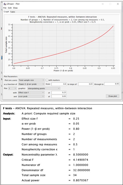
“A full randomized block design was used to assign participants to both groups (active neuromodulation group, NM; sham-control group, SC) (see Fig. 2C). As the pilot study probing into the effect of single-session tDCS stimulation to change procrastination willingness indicated (t = 2.38, p = .02, 95% CI [0.14, 1.49]; Xu et al., 2023), statistical power was predetermined by G*Power at a relatively medium effect size (1-β err prob = 0.80, f = 0.25), yielding the total sample size at 18 to reach acceptable power (see SM Methods and Fig. S1)....”
We fully understand that this sample size to reach a medium effect size is seemingly low, and that the18 participants for each group are apparently limited in any case. Upon double-checking these power analyses, we confirmed that this sample size requirement is indeed correct. Please see the G*Power outputs in Author response image 1.
Author response image 1.
Despite the absence of algorithmic errors in the power analysis here, we are aware that this limited sample size may hamper statistical robustness. To tackle this weakness, we have clearly warranted such cautions in the Limitation section:
Limitations Section (Page 12, Line 637-640)
“... In addition to technical limitations, given the apparently limited size of the sample (total N = 46), it warrants caution in generalizing these findings elsewhere, and necessitates further validations in a large-scale cohort.”
(5) It remains somewhat ambiguous whether the sham group had the same number of stimulation sessions as the verum stimulation group; please clarify: Did both groups come in the same number of times into the lab? I.e., were all procedures identical except whether the stimulation was verum or sham?
Yes, we fully followed the CONSORT pipeline to carry out this double-blind trial, and thus confirmed that all the participants in both groups had the same number of stimulation sessions in our lab. That is to say, except for the stimulation type (verum vs sham), all the procedures, equipment and even the room were identical for all the participants. For clarification, we have clearly stated this in the main text:
Results Section (Page 9, Line 419-423)
“In both groups, almost all participants (93.2%, 41/44) reported perceiving acceptable pain stemming from current stimulation, and believed they were receiving treatment (91.30% (21/23) for active neuromodulation group (NM), 86.95% (20/23) for sham control group (SC), x<sup>2</sup> = 0.224, p = .636). All the participants were engaged in the identical experimental procedures excepting to stimulation’s type (active vs sham). ...”
(6) The TDM analysis and hyperbolic discounting approach were unclear to me; this needs to be described in more detail, otherwise it cannot be evaluated.
We apologize for the inadequate details, which hindered a precise understanding of the TDM and the hyperbolic discounting model. The Temporal Decision Model (TDM) was originally proposed by our team (Xu et al., 2023; Zhang et al., 2019, 2020, 2021), which theoretically conceptualizes procrastination as the failure of trade-off between task outcome value (i.e., motivation to take actions now for pursuing task reward) and task aversiveness (i.e., motivations to take away from playing actions now for avoiding negative experiences). Once task aversiveness overrides the pursuit of task outcome values, the procrastination emerges. One overarching hypothesis in this theoretical model is that the task aversiveness is hyperbolically discounted when approaching the deadline: it would be discounted sharply when far from the deadline but discounted slowly when nearing the deadline (Zhang et al., 2019). Considering the nonlinear dynamics inherent in this hyperbolic discounting, we therefore employed a log-spaced temporal sampling scheme (Myerson et al., 2001) to strengthen curve-fitting performance (please see the schematic diagram (https://uen.pressbooks.pub/behavioraleconomics/chapter/the-reality-of-homo-sapiens, where each point indicates a sampling time)):
Specifically, based on the log-spaced temporal sampling rule, five time points were first selected to fulfill the statistical prerequisites for hyperbolic model fitting, with increasing sampling density toward the deadline (e.g., for a task due at 20:00: sampling occurred at 10:00, 16:00, 18:00, 19:30, 20:00). At each time point, participants reported task aversiveness (A) on a 0–100 Visual Analog Scale (VAS). Then, task aversiveness discounting was calculated as 1- (A<sub>t</sub> / A<sub>earliest</sub>), where t<sub>earliest</sub> was the earliest sampling point (e.g., 10:00), serving as the reference for immediate execution. Subsequently, using the GraphPad Prisma software (v9, 525), we estimated the AUC from these five data points based on the Myerson algorithm (Myerson et al., 2001), which was computed as the trapezoidal integration of task aversiveness discounting over time. By this modelling method, a higher AUC reflects stronger temporal discounting of task aversiveness, which means that participants experience a faster decline in subjective aversiveness as execution is delayed, yielding lower effective aversiveness and reduced avoidance behavior. That is to say, if a participant showcases a greater discounting of task aversiveness as reflected by a higher AUC, she/he experiences a more pronounced reduction in subjective aversiveness upon postponement, plausibly yielding less procrastination. As you kindly suggested, we have added these details to explicitly clarify how to use the hyperbolic discounting approach for determining sampling time points and for calculating AUC of task aversiveness discounting.
Methods Section (Page 6, Line 268-283)
“On the Task day, we developed a mobile app to implement experience sampling method (ESM) for tracking one’s real-time evaluation of task aversiveness and task outcome value (see Fig. 1). The task aversiveness describes how disagreeable one perceives when performing a given real-life task to be, whereas outcome value refers to the subjective benefits of the task outcome brought about by completing the task before the deadline (Zhang & Feng, 2020). As theoretically conceptualized by the temporal decision model (TDM) of procrastination, the perceived task aversiveness is hyperbolically discounted when approaching deadline, showing sharply discounting when faring away from deadline but slowly discounting once nearing deadline (Zhang & Feng, 2020; Zhang et al., 2021). Thus, considering this nonlinear dynamics inherent in this hyperbolic discounting, the five recording moments of ESM were selected per task a priori by using a log-spaced temporal sampling scheme (Myerson et al., 2001), with increasing sampling density toward the deadline, such as moments of 10:00 (earliest), 16:00, 18:00, 19:30, 20:00 (deadline). The five sampling points could meet statistical prerequisite in the hyperbolic model fitting, requiring ≥ 4 points (Green & Myerson, 2004). To do so, recording moments of tasks were individually tailored for each task per participant in this ESM procedure.”
Methods Section (Page 7, Line 318-334)
“... As articulated temporal decision theoretical model above, the task aversiveness evoked by executing a task was temporally dynamic in a hyperbolic discounting pattern, with sharply discounting in faring away from deadline but slowly discounting in nearing deadline (Zhang & Feng, 2020). To quantitatively characterize the task aversiveness with consideration for its dynamics, the model-free area under the curve (AUC) was calculated. Specifically, based on the log-spaced temporal sampling rule, task aversiveness was measured by 100-point visual analog scale at the five sampling moments. Then, the task aversiveness discounting (A) was calculated as 1- (A(t) / A(earliest)), where t(earliest) was the earliest sampling point, serving as the reference for immediate execution. Subsequently, using the GraphPad Prisma software (v9, 525), the AUC was computed as the trapezoidal integration between task aversiveness discounting and time across five data points, basing on the Myerson algorithm (Myerson et al., 2001). By doing so, a higher AUC reflects stronger temporal discounting of task aversiveness along with nearing deadline, which means that participants experience a faster decline in subjective aversiveness as execution is delayed, yielding lower effective aversiveness and reduced avoidance behavior. As for the task outcome value, it was theoretically posited as a relatively stable evaluation of the task (Zhang & Feng, 2020; Zhang et al., 2021).”
References
Myerson, J., Green, L., & Warusawitharana, M. (2001). Area under the curve as a measure of discounting. Journal of the experimental analysis of behavior, 76(2), 235–243. https://doi.org/10.1901/jeab.2001.76-235
Xu, T., Zhang, S., Zhou, F., & Feng, T. (2023). Stimulation of left dorsolateral prefrontal cortex enhances willingness for task completion by amplifying task outcome value. Journal of experimental psychology. General, 152(4), 1122–1133. https://doi.org/10.1037/xge0001312
Zhang, S., Verguts, T., Zhang, C., Feng, P., Chen, Q., & Feng, T. (2021). Outcome Value and Task Aversiveness Impact Task Procrastination through Separate Neural Pathways. Cerebral cortex (New York, N.Y. : 1991), 31(8), 3846–3855. https://doi.org/10.1093/cercor/bhab053
Zhang, S., Liu, P., & Feng, T. (2019). To do it now or later: The cognitive mechanisms and neural substrates underlying procrastination. Wiley interdisciplinary reviews. Cognitive science, 10(4), e1492. https://doi.org/10.1002/wcs.1492
Zhang, S., & Feng, T. (2020). Modeling procrastination: Asymmetric decisions to act between the present and the future. Journal of experimental psychology. General, 149(2), 311–322. https://doi.org/10.1037/xge0000643
(7) Coming back to the point about the statistical analyses not being described in enough detail: One important example of this is the inclusion of random slopes in their mixed-effects model which is unclear. This is highly relevant as omission of random slopes has been repeatedly shown that it can lead to extremely inflated Type 1 errors (e.g., inflating Type 1 errors by a factor of then, e.g., a significant p value of .05 might be obtained when the true p value is .5). Thus, if indeed random slopes have been omitted, then it is possible that significant effects are significant only due to inflated Type 1 error. Without more information about the models, this cannot be ruled out.
Thank you for sharing this very timely and crucial comment. After careful scrutiny, we identified this statistical flaw you pointed out - each participant was not yet modeled as random slopes but as random intercepts merely. As you kindly suggested, we have reanalyzed all the statistics by adding random slopes (i.e., (1 + day|SubjectID)). Results showed a statistically significant interaction effect for both procrastination willingness (β = -7.8, SE = 1.8, DF = 45.6, p < .001) and actual procrastination rates (β = -7.4, SE = 2.4, DF = 46.6, p = .004), indicating the effectiveness of multi-session neuromodulation in mitigating procrastination. In the post-hoc simple effect analyses, participants who engaged in active neuromodulation (NM) showed a significant increase in task-execution willingness (i.e., decreased procrastination willingness; NM-before: 35.65 ± 30.20, NM-after: 80.43 ± 19.92, t.ratio = 5.4, p < .0001, Tukey correction) and a decrease in actual procrastination rates (NM-before: 43.26 ± 39.09, NM-after: 0.00 ± 0.00, t.ratio = 5.1, p < .0001, Tukey correction), while no such effects were identified for participants in the sham control group (for willingness, SC-before: 37.57 ± 26.46, SC-after: 47.35 ± 30.49, t.ratio =0.3, p = .77, Tukey correction; for actual procrastination, SC-before: 46.47 ± 40.75, SC-after: 33.34 ± 37.82, t.ratio = 0.7, p = .48, Tukey correction). Taken together, we do appreciate your pointing out this definitely crucial statistical weakness, and have confirmed that our findings remain reliable after adjusting for Type 1 error by adding random slopes. Moreover, as you kindly suggested, we have incorporated these statistical details, particularly those concerning the GLMM, into the main text to facilitate your evaluation. Please see specific revisions below:
Methods Section (Page 8, Line 381-401)
“To clarify whether multiple-session HD-tDCS neuromodulation can reduce procrastination, the generalized mixed-effects linear model (GLMM) was constructed with full factorial design for subjective procrastination willingness (i.e., self-reported visual analog scores) and actual procrastination behavior (i.e., real-world task-completion rate before deadline). Here, sex, age and socioeconomic status (SES) were modeled as covariates of no interest. As the National Bureau of Statistics (China) issued (https://www.stats.gov.cn/sj/tjbz/gjtjbz/), on the basis of per capita annual household income, the SES was divided into seven hierarchical tiers from 1 (poor) to 7 (rich). To obviate subjective rating bias stemming from individual daily mood, we separately measured participants’ daily emotional fluctuation at 10:00 and 16:00 using a self-rating visual analog item (i.e., “How do feel for your mood today?”, 0 for “completely uncomfortable” and 100 for “definitely happy”). By doing so, the averaged score of those self-rating emotions at the two time points was modeled into the GLMM as covariate of no interests, yielding the final expression of “outcome ~ Group*Treatment_Day + Age + Gender + SES + Emotions + (1 + Treatment_Day | SubjectID)” in the statistical model”. This analysis was implemented using the “lme4” and “lmerTest” packages. Employing “emmeans” package, simple effects were also tested at baseline and post-last-intervention using Tukey-adjusted pairwise comparisons of estimated marginal means from the full GLMM, controlling for covariates and random-effects structure. To validate statistical robustness, instead of continuous outcomes for parametric tests, we also conducted a between-group comparison for the number of tasks that procrastination emerges by using the nonparametric x<sup>2</sup> test with φ correction or Fisher exact test....”
Results Section (Page 9, Line 428-449)
“To identify whether ms-tDCS targeting the left DLPFC can alleviate subjective procrastination willingness and actual procrastination behavior, a generalized linear mixed-effects model with Scatterthwaite algorithm was built, with task-execution willingness and actual procrastination rates (PR) as primary outcomes, respectively. For procrastination willingness, results showed a statistically significant interaction effect between multi-session neuromodulations and groups (β = -7.8, SE = 1.8, DF = 45.6, p < .001; Fig. 3A). In the post-hoc simple effect analysis, it demonstrated a significantly increased task-execution willingness (i.e., decreased procrastination willingness) after neuromodulation in the active neuromodulation group (NM-before: 35.65 ± 30.20, NM-after: 80.43 ± 19.92, t.ratio = 5.4, p < .0001, Tukey correction), but no such effects were identified in the sham control group (SC-before: 37.57 ± 26.46, SC-after: 47.35 ± 30.49, t.ratio =0.3, p = .77, Tukey correction) (Fig. 3B-C). A linear uptrend for task-execution willingness was further observed across multiple sessions in the active NM group, indicating gradually increasing neuromodulation effects (Fig. 3D; p < .01, Mann-Kendall test). For actual procrastination behavior, changes to actual procrastination rates across all the sessions have been detailed in the Fig. 3E. Similarly, a statistically significant interaction effect was identified here (β = -7.4, SE = 2.4, DF = 46.6, p = .004), and the simple effect analysis further revealed decreased actual procrastination rates after ms-tDCS in the active neuromodulation group (NM-before: 43.26 ± 39.09, NM-after: 0.00 ± 0.00, t.ratio = 5.1, p < .0001, Tukey correction), but no such prominent changes found in the sham control group (SC-before: 46.47 ± 40.75, SC-after: 33.34 ± 37.82, t.ratio = 0.7, p = .48, Tukey correction) (Fig. 3F-G). Also, a significant downtrend for procrastination rates across all the sessions was identified in the active NM group (Fig. 3H; p < .01, Mann-Kendall test).”
(8) Related to the previous point: The authors report, for example, on the first results page, line 420, an F-test as F(1, 269). This means the test has 269 residual degrees of freedom despite a sample size of about 50 participants. This likely suggests that relevant random slopes for this test were omitted, meaning that this statistical test likely suffers from inflated Type 1 error, and the reported p-value < .001 might be severely inflated. If that is the case, each observation was treated as independent instead of accounting for the nestedness of data within participants. The authors should check this carefully for this and all other statistical tests using mixed-effects models.
Thank you for underlining this very timely and helpful comment. As you correctly pointed out above, we did not include random slopes in the original GLMM, highly risking the inflation of the false-positive rate (i.e., Type-I error). By adding the random slopes, we reanalyzed all the statistics from the GLMM, and confirmed that all the findings are still reliable from those new GLMMs with random slopes. Again, thank you for this crucial statistical advice, and please see the above response for full details regarding what we have revised to address this comment you kindly raised.
(9) Many of the statistical procedures seem quite complex and hard to follow. If the results are indeed so robust as they are presented to be, would it make sense to use simpler analysis approaches (perhaps in addition to the complex ones) that are easier for the average reader to understand and comprehend?
We do thank you for this practical and helpful comment. In the original manuscript, we incorporated a joint model of longitudinal and survival data (JM-LSD), in conjunction with machine learning algorithms, to strengthen the robustness of our statistical findings. Nevertheless, we all agree with you on this point: there is no need to complicate the analyses by repeatedly probing the same research question to increase methodological robustness, at the expense of compromising readability and intelligibility for a broader audience. As you suggested, we have removed these complicated statistical methods, and merely maintained the primary ones - GLMM and X<sup>2</sup> cross-tab test, as well as a complementary one - Mann-Kendall linear trend test. Thus, we have almost rewritten the whole Results section. Please see the specific instances below:
Results Section (Page 9, Line 468-485)
“Ms-tDCS changes task aversiveness and task-outcome value
Both task aversiveness and task outcome value serve as key pathways determining whether one would procrastinate. To this end, we further utilized a generalized linear mixed-effects model to examine the effects of ms-tDCS on changes in task aversiveness and task outcome value. Task aversiveness changes across all the sessions are shown in the Fig. 4A and 4C. We demonstrated a statistically significant decrease in task aversiveness and an increase in task outcome value via ms-tDCS in the neuromodulation group (Task aversiveness: interaction effect, β = -0.12, SE = 0.04, DF = 46.7, p = .002; simple effect, NM-before <sub>(AUC)</sub>: 1.13 ± 0.53, NM-after <sub>(AUC)</sub>: 1.95 ± 0.85, t.ratio = 4.5, p < .001, Tukey correction; Outcome value: β = -6.8, SE = 1.74, DF = 46.2, p < .001; simple effect, NM-before: 35.86 ± 27.82, NM-after: 73.08 ± 23.33, t.ratio = 5.0, p < .001, Tukey correction; see Fig. 4B), but not in the sham control group (Task aversiveness: SC-before <sub>(AUC)</sub>: 1.07 ± 0.51, SC-after <sub>(AUC)</sub>: 1.28 ± 0.46, t.ratio = 1.3, p = .20, Tukey correction; Outcome value: SC-before: 34.00 ± 25.17, SC-after: 40.13 ± 28.94, t.ratio = 0.8, p = .41, Tukey correction; see Fig. 4D). In the neuromodulation (NM) group, task aversiveness steadily decreased with the cumulative number of stimulation sessions, while perceived task outcome value increased significantly (see Fig. 4E-F, p < .05, Mann-Kendall test). Thus, it provides causal evidence clarifying that neuromodulation to left DLPFC reduces task aversiveness and enhances task-outcome value meanwhile.”
Results Section (Page 10, Line 525-542)
“Long-term effects of ms-tDCS
We have also attempted to conduct a follow-up investigation to test the long-term retention of ms-tDCS in reducing actual procrastination. Almost all the participants had undergone follow-up except one in the neuromodulation group after last neuromodulation for 6 months (N<sub>NM</sub> = 22, N<sub>SC</sub> = 23). Thus, the GLMM was constructed, with the PR before first neuromodulation vs. PR after last neuromodulation for 6 months as covariates of interest. Results showed the statistically significant group*time interaction effects (β = 16.5, SE = 9.9, p = .049). Simple-effect model demonstrated a decrease in actual procrastination rates in the active neuromodulation group after last stimulation for 6 months compared to baseline (β = -22.05, SE = 10.0, p = .038, Tukey correction; NM-before: 40.68 ± 37.96, NM-after<sub>6-months</sub>: 18.63 ± 29.80), and revealed null effects in the SC group (β = 1.26, SE = 9.78, p = .99, Tukey correction; SC-before: 46.47 ± 40.75, SC-after<sub>6-months</sub>: 47.73 ± 39.18) (see Fig. 6).. Furthermore, using a nonparametric x<sup>2</sup> test to compare differences in the number of procrastinated tasks, we still found a statistically significant reduction in procrastination frequency in NM group after neuromodulation for 6 months compared to baseline (x<sup>2</sup> = 3.30, p = .035, NM-before: 68.19% (15/22), NM-after<sub>6-months</sub>: 40.91% (9/22)), while no significant changes were observed in the SC group (x<sup>2</sup> = 0.11, p = .74, SC-before: 69.56% (16/23), SC-after<sub>6-months</sub>: 73.91% (17/23)). Therefore, beyond to short-term effects, the benefits of ms-tDCS neuromodulation to reduce procrastination pose the long-term retention.”
(10) As was noted by an earlier reviewer, the paper reports nearly exclusively about the role of the left DLPFC, while there is also work that demonstrates the role of the right DLPFC in self-control. A more balanced presentation of the relevant scientific literature would be desirable.
We are grateful to you for noticing the unbalanced presentation of the literature on left DLPFC. As you kindly suggested, we have added literature to support the association between self-control and the right lateralization of the DLPFC. Please see below for what we have revised:
Introduction Section (Page 4, Line 137-143)
“...In addition to the left lateralization, there is solid evidence indicating significant associations between self-control and the right DLPFC indeed, particularly given that this region specifically functions in top-down regulation, future self-continuity representation and social decisions (Huang et al., 2025; Lin and Feng, 2024; Knoch & Fehr, 2007). Despite this case, Xu and colleagues demonstrated null effects of anodally stimulating the right DPFC to modulate either value evaluation or emotional regulation for changing procrastination willingness (Xu et al., 2023).”
(11) Active stimulation reduced procrastination, reduced task aversiveness, and increased the outcome value. If I am not mistaken, the authors claim based on these results that the brain stimulation effect operates via self-control, but - unless I missed it - the authors do not have any direct evidence (such as measures or specific task measures) that actually capture self-control. Thus, that self-control is involved seems speculation, but there is no empirical evidence for this; or am I mistaken about this? If that is indeed correct, I think it needs to be made explicit that it is an untested assumption (which might be very plausible, but it is still in the current study not empirically tested) that self-control plays any role in the reported results.
We truly appreciate your pointing out this weakness with regard to conceptualization. Yes, you are correct in understanding this causal chain: we conceptually speculate that the HD-tDCS stimulation over the left DLPFC operates self-control to change procrastination, rather than empirically validating this component in the chain: brain stimulation→increased self-control→increased task outcome value→decreased procrastination. In this causal chain, we did not collect data to directly measure self-control at either baseline or post-neuromodulation times. Therefore, we all agree with your suggestion to explicitly claim this case in the main text. Following this advice, we have redrawn a portion of the Conclusion by clearly pointing out the hypothesis-generating role of self-control in mitigating procrastination, and have further claimed this case in the Limitation section:
Abstract Section (Page 2, Line 55-57)
“... This establishes a precise, value-driven neurocognitive pathway to account the conceptualized roles of self-control on procrastination, and offers a validated, theory-driven strategy for interventions.”
Results Section (Page 10, Line 489-492 and 520-522)
“Given the dual neurocognitive pathways identified above—reduced task aversiveness and increased task-outcome value—we proposed that these changes, conceptually driven by enhanced self-control via ms-tDCS over left DLPFC, account for how neuromodulation reduces procrastination. ...”
“In summary, these findings demonstrated a mechanistic pathway underlying procrastination: the self-control that was conceptualized to be governed by left DLPFC mitigate procrastination by plausibly increasing task-outcome value.”
Discussion Section (Page 13, Line 642-645)
“Moreover, this study did not collect data for assessing participants’ self-control at either baseline or post-neuromodulation, thereby limiting our ability to determine whether the effects on procrastination were uniquely attributable to neuromodulation-induced changes in self-control. ...”
(12) Figures 3F and 3H show that procrastination rates in the active modulation group go to 0 in all participants by sessions 6 and 7. This seems surprising and, to be honest, rather unlikely that there is absolutely no individual variation in this group anymore. In any case, this is quite extraordinary and should be explicitly discussed, if this is indeed correct: What might be the reasons that this is such an extreme pattern? Just a random fluctuation? Are the results robust if these extreme cells are ignored? The authors remove other cells in their design due to unusual patterns, so perhaps the same should be done here, at least as a robustness check.
Thank you for raising this highly important and helpful comment. Indeed, we fully understand that this result is somewhat extraordinary, a fact that was equally striking to us when unblinding the data. After carefully scrutinizing the data and statistics, we are thrilled to confirm that this pattern is true. In support of this observation, we were gratified to receive numerous thank-you letters from participants who engaged in active neuromodulation. They expressed gratitude to us, and reported that they have substantially ameliorated procrastination behavior in real-life activities after completing the trial. While this does not constitute formal scientific evidence, we are also glad to see the benefits of this neuromodulation for those procrastinators.
Two reasons could account for this pattern herein. One interpretation is to attribute this pattern to “scalar inflation”. In the present study, the procrastination rate was calculated as 1 minus the task-completion rate (e.g., 80%, 60%, 40%) by the deadline. At sessions # 6 and #7, all the participants completed their real-life tasks before the deadline, yielding a 0% (1 minus 100% completion rate) procrastination rate, without any between-individual variation. Thus, rather than there being no individual variation in procrastination, this scalar – the procrastination rate - is too insensitive to capture subtle differences per se. For instance, although participants #1 and #2 both showed a 0% procrastination rate - meaning that both completed their tasks before the deadline - Participant #1 might have completed it 3 hours before the deadline, whereas Participant #2 might have completed it only 10 minutes before. In this case, the “scalar inflation” emerges to let us perceive that both participants have equivalent procrastination rates, although participant #2 may have a higher procrastination level than #1. As conceptually defined in the field, procrastination is contextualized as “not completing a task before the deadline”. Thus, if this task is completed before the deadline, regardless of whether it was finished close to or far in advance of the deadline, this case is defined as “no procrastination”. In the present study, the primary outcome is whether a participant procrastinated on a real-life task before the deadline in real-world settings, irrespective of when she/he completed this task. Thus, this scalar - procrastination rate - fits our conceptualization of procrastination.
Another reason is the potential accumulative effects from sequential multi-session tDCS stimulation. As shown in Mann-Kendall trend tests, the procrastination rates show a significant linear downtrend in the active neuromodulation group across sessions, even after removing sessions #6 and #7. This indicates that the improvements of going against procrastination may be sequentially accumulative along with the increase in sessions, implying a potential “dose-dependent effect”. Despite a speculative interpretation, this “dose-dependent effect” in neuromodulation has been well-documented in previous studies, showing the robustly linear association between the number of sessions and effectiveness (c.f., Cole et al., 2020; Hutton et al., 2023; Sabé et al., 2024; Schulze et al., 2018). Therefore, although this extreme pattern is somewhat extraordinary compared to previous observations, it makes sense.
Yes, this is a definitely great idea to carry out a robustness check by removing sessions #6, #7, or both. We do believe that this analysis could support statistical robustness to go against potential biases from extreme cells. By doing so, we found that all the group*treatment_day interaction effects remained significant when removing either session #6 or session #7 (or even both, all p-values < .05), indicating high statistical robustness. Please see Supplementary table S3 and S4
Taken together, in spite of their being extraordinary, we confirm that those findings are statistically robust to extreme outliers. As you kindly suggested, we have added those findings of the robustness check into the revised Supplemental Materials section.
References
Cole, E. J., Stimpson, K. H., Bentzley, B. S., Gulser, M., Cherian, K., Tischler, C., Nejad, R., Pankow, H., Choi, E., Aaron, H., Espil, F. M., Pannu, J., Xiao, X., Duvio, D., Solvason, H. B., Hawkins, J., Guerra, A., Jo, B., Raj, K. S., Phillips, A. L., … Williams, N. R. (2020). Stanford Accelerated Intelligent Neuromodulation Therapy for Treatment-Resistant Depression. The American journal of psychiatry, 177(8), 716–726. https://doi.org/10.1176/appi.ajp.2019.19070720
Hutton, T. M., Aaronson, S. T., Carpenter, L. L., Pages, K., Krantz, D., Lucas, L., Chen, B., & Sackeim, H. A. (2023). Dosing transcranial magnetic stimulation in major depressive disorder: Relations between number of treatment sessions and effectiveness in a large patient registry. Brain stimulation, 16(5), 1510–1521. https://doi.org/10.1016/j.brs.2023.10.001
Sabé, M., Hyde, J., Cramer, C., Eberhard, A., Crippa, A., Brunoni, A. R., Aleman, A., Kaiser, S., Baldwin, D. S., Garner, M., Sentissi, O., Fiedorowicz, J. G., Brandt, V., Cortese, S., & Solmi, M. (2024). Transcranial Magnetic Stimulation and Transcranial Direct Current Stimulation Across Mental Disorders: A Systematic Review and Dose-Response Meta-Analysis. JAMA network open, 7(5), e2412616. https://doi.org/10.1001/jamanetworkopen.2024.12616
Schulze, L., Feffer, K., Lozano, C., Giacobbe, P., Daskalakis, Z. J., Blumberger, D. M., & Downar, J. (2018). Number of pulses or number of sessions? An open-label study of trajectories of improvement for once-vs. twice-daily dorsomedial prefrontal rTMS in major depression. Brain stimulation, 11(2), 327–336. https://doi.org/10.1016/j.brs.2017.11.002
(13) The supplemental materials, unfortunately, do not give more information, which would be needed to understand the analyses the authors actually conducted. I had hoped I would find the missing information there, but it's not there.
Sorry to offer uninformative supplemental materials (SM) in the original submission. As you suggested, we have added a substantial number of details to clarify how we conducted data analyses in the main text, and also tightened the whole SM section to improve readability and comprehensibility. We do hope that this revised manuscript could offer clear and adequate information in understanding methods and statistics for broader readers.
In sum, the reported/cited/discussed literature gives the impression of being incomplete/selectively reported; the analyses are not reported sufficiently transparently/fully to evaluate whether they are appropriate and thus whether the results are trustworthy or not. At least some of the patterns in the results seem highly unlikely (0 procrastination in the verum group in the last 2 observation periods), and the sample size seems very small for a between-subjects design.
Thank you for this very helpful summary. As you kindly suggested above, we have overhauled this manuscript to address those points that you listed here, particularly where we added relevant literature to balance our claims, added a huge amount of details to sufficiently/transparently report statistics, and conducted a robustness check to confirm the statistical robustness of our findings to those plausible extreme patterns (sessions #6 and #7), as well as justified how we determined this sample size fulfilling medium statistical power in a priori. Please see above for full details regarding how we addressed those comments, point-by-point.
Reviewer #2 (Public Review):
Chen and colleagues conducted a cross-sectional longitudinal study, administering high-definition transcranial direct stimulation targeting the left DLPFC to examine the effect of HD-tDCS on real-world procrastination behavior. They find that seven sessions of active neuromodulation to the left DLPFC elicited greater modulation of procrastination measures (e.g., task-execution willingness, procrastination rates, task aversiveness, outcome value) relative to sham. They report that tDCS effects on task-execution willingness and procrastination are mediated by task outcome value and claim that this neuromodulatory intervention reduces procrastination rates quantified by their task. Although the study addresses an interesting question regarding the role of DLPFC on procrastination, concerns about the validity of the procrastination moderate enthusiasm for the study and limit the interpretability of the mechanism underlying the reported findings.
Strengths:
(1) This is a well-designed protocol with rigorous administration of high-definition transcranial direct current stimulation across multiple sessions. The approach is solid and aims to address an important question regarding the putative role of DLPFC in modulating chronic procrastination behavior.
(2) The quantification of task aversiveness through AUC metrics is a clever approach to account for the temporal dynamics of task aversiveness, which is notoriously difficult to quantify.
Thank you for taking your invaluable time to review our manuscript, warmly applauding the strength in research design and the conceptualization of scaling task aversiveness, as well as kindly sharing such helpful and insightful evaluations. As you correctly pointed out, we are aware of the absence of detailed, clear and understandable reporting of measures (e.g., real-world procrastination), statistics and methods, in the original manuscript. Following all your suggestions, we have thoroughly revised this manuscript to address those comments that you kindly made, point-by-point. Please see the full response underneath.
Weaknesses:
(1) The lack of specificity surrounding the "real-world measures" of procrastination is problematic and undermines the strength of the evidence surrounding the DLPFC effects on procrastination behavior. It would be helpful to detail what "real-world tasks" individuals reported, which would inform the efficacy of the intervention on procrastination performance across the diversity of tasks. It is also unclear when and how tasks were reported using the ESM procedure. Providing greater detail of these measures overall would enhance the paper's impact.
We genuinely appreciate your raising this very crucial comment. We are sorry for omitting a tremendous number of methodological details to comply with the editorial requirement on the manuscript’s length, which hampered the comprehension of how we measure “real-life tasks” and “real-world procrastination”.
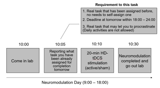
As shown in the schematic diagram for experimental procedure (Fig. 1), the experimental protocol alternated between Neuromodulation Days (Days 2, 4, 6, 8, 10, 12, 14) and Task Days (Days 1, 3, 5, 7, 9, 11, 13, 15). On each Neuromodulation Day, participants received either active or sham HD-tDCS, and—critically—before stimulation—were instructed to specify a real-life task they were required to complete the following day, with a deadline between 18:00 and 24:00. This ensured ≥24 hours between neuromodulation and task execution, isolating offline after-effects. For instance, on Day #2 (Neuromodulation Day), before carrying out stimulation, participants were asked to report a real-life task that has a deadline within 18:00 - 24:00 for tomorrow’s “task day” (Day #3) (please see the schematic diagram in Author response image 2).
Author response image 2.
There are some real-life tasks that they reported in our experiment as examples: “Complete and submit a homework assignment”, “Complete a standardized English proficiency test”, “Complete an online course module required for applying a Class C driver’s license”, “Prepare slides for a seminar presentation”, “Practice guitar”, “Practice Chinese calligraphy”, and “Do the laundry”. Reported tasks spanned academic (e.g., submitting an assignment), occupational (e.g., preparing a presentation), administrative (e.g., applying for a license), self-improvement (e.g., practicing guitar for ≥30 min), domestic (e.g., laundry), and health-related domains (e.g., running ≥ 2,000m for exercise), indicating a plausible task diversity.
On each “task day”, participants engaged in an intensive Experience Sampling Method (iESM) protocol via a custom-built mobile app. Using this app, participants were required to report a subjective task-execution willingness score (i.e., a one-item 100-point visual analog scale, “How willing are you to do this task?”, 0 for “I will definitely procrastinate this task” and 100 for “I will take action to complete this task immediately”; procrastination willingness = 100 – the task-execution willingness score), the subjective task aversiveness (i.e., a one-item 100-point visual analog scale), the subjective task outcome value (i.e., a one-item 100-point visual analog scale), and the objective procrastination rate, respectively.
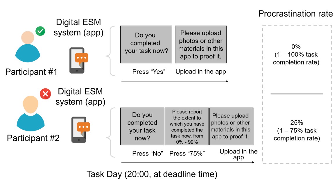
Rather than self-reported scores from those one-item visual analog scales, we asked participants to report real “task completion rate” for the objective quantification of the “real-world procrastination behavior”. Specifically, at the deadline, each participant was asked to report whether she/he had completed this task. If she/he reported not having yet completed the task (i.e. procrastination behavior emerged), she/he was further required to report the percentage of the task completed (1% - 99%), which was defined as the task completion rate. By doing so, we could calculate the real-world procrastination rate for the real-life task as the “1 – the task completion rate”. For instance, if a participant did not complete her/his real-life task before the deadline (i.e. she/he procrastinated this task) and reported completing 75% of this task at the deadline, her/his real-world procrastination rate was computed as the 25% (1 - 75%) (Please see the schematic diagram in Author response image 3).
Moreover, rather than merely a self-reported task completion rate, each participant was also asked to upload proof (e.g., screenshots of submitted assignments, photos of printed documents, system timestamps) to the ESM digital system for validation.
Author response image 3.
To determine the sampling time points for this mobile app in the ESM, we capitalized on both the conceptual temporal decision model and the statistical Myerson algorithm. Specifically, the Temporal Decision Model (TDM) was originally proposed by our team (Xu et al., 2023; Zhang et al., 2019, 2020, 2021), which theoretically conceptualizes procrastination as the failure of the trade-off between task outcome value (i.e., motivation to take actions now for pursuing task reward) and task aversiveness (i.e., motivations for avoiding taking action now for avoiding negative experiences). Once task aversiveness overrides the pursuits of task outcome values, procrastination emerges. One overarching hypothesis in this theoretical model is that the task aversiveness is hyperbolically discounted when approaching the deadline: it would be discounted sharply when far from the deadline but discounted slowly when nearing the deadline (Zhang et al., 2019). To maximize statistical power to fit dynamic motivational curves, we employed a log-spaced temporal sampling scheme (Myerson et al., 2001) (please see the schematic diagram in https://uen.pressbooks.pub/behavioraleconomics/chapter/the-reality-of-homo-sapiens, where each point indicates a sampling time):
By this fitting algorithm (Myerson et al., 2001), five time points were selected to fulfill the statistical prerequisites for hyperbolic model fitting, with increasing sampling density toward the deadline (e.g., for a task due at 20:00: sampled at 10:00, 16:00, 18:00, 19:30, 20:00). Once the task-specific five sampling time points were determined per participant, this mobile app sent a digital message to ask her/him to immediately report the task aversiveness and the task outcome value then. As the primary outcomes, the procrastination rate (i.e., 1 – the task completion rate) and the procrastination willingness were sampled at the deadline point.
Furthermore, yes, we fully concur with you on this great idea, that is, transparency about task diversity strengthens the generalizability of our findings. In response, we have tabulated these real-life tasks that were reported in this experiment in the independent Appendix 1, with automatic translations from Chinese to English via Qwen GPT. Please see below for what we have added to the main text:
Methods Section (Page 6-7, Line 238-308)
“Nested cross-sectional longitudinal design
This study used a nested cross-sectional longitudinal design to investigate whether the multiple-session anodal HD-tDCS targeting the left DLPFC could reduce actual procrastination behavior and to probe how this effect manifests. To assess procrastination in daily life, we implemented a 15-day protocol alternating between Neuromodulation Days (Days 2, 4, 6, 8, 10, 12, 14) and Task Days (Days 1, 3, 5, 7, 9, 11, 13, 15). On the Neuromodulation days, the 20-min anodal HD-tDCS neuromodulation targeting the left DLPFC was performed for HD-tDCS active group at intervals of 2 days, while the sham-control group received sham HD-tDCS training. This HD-tDCS training was repeated for a total of seven sessions, and lasted 15 days (see Fig. 1a). Crucially, to capture procrastination in ecologically valid contexts, prior to receiving either active or sham HD-tDCS (administered between 09:00–18:00), participants were instructed to specify a real-life task they were personally obligated to complete the following day, with a self-defined deadline strictly constrained to 18:00–24:00 to ensure ≥24 hours between stimulation offset and task deadline, thereby isolating offline after-effects. This task should meet the following three criteria: (a) it should be already assigned in the real-world settings; (b) deadline should be constrained to 18:00-24:00 (see above); (c) it should be more likely to induce procrastinate. By doing so, more than 300 real-life tasks were collected, spanning academic (e.g., “submit a statistics homework assignment”), occupational (e.g., “draft and email a project proposal”), administrative (e.g., “complete online application for Class C driver’s license”), self-improvement (e.g., “practice guitar for ≥30 minutes”), domestic (e.g., “do laundry ”), and health-related (e.g., “running 2,000m for exercise”). Full task list has been tabulated in the Appendix 1. As primary outcomes, all the participants were required to reported task-execution willingness (TEW) (Zhang & Feng, 2020; Zhang, Liu, et al., 2019), for a real-life task 24 hours post-neuromodulation. Thus, procrastination willingness was quantified as 100-TEW score (see underneath for details). Furthermore, we asked participants to report the actual task completion rate (CR) of the task at the deadline (e.g. participant A finished 90% homework at deadline and reported this situation to us at deadline). In this vein, the actual procrastination rate (PR) was quantified as 1-CR.
On the Task day, we developed a mobile app to implement experience sampling method (ESM) for tracking one’s real-time evaluation of task aversiveness and task outcome value (see Fig. 1). The task aversiveness describes how disagreeable one perceives performing a given real-life task to be, whereas outcome value refers to the subjective benefits of the task outcome brought about by completing the task before the deadline (Zhang & Feng, 2020). As theoretically conceptualized by the temporal decision model (TDM) of procrastination, the perceived task aversiveness is hyperbolically discounted when approaching deadline, showing sharply discounting when faring away from deadline but slowly discounting once nearing deadline (Zhang & Feng, 2020; Zhang et al., 2021). Thus, considering this nonlinear dynamics inherent in this hyperbolic discounting, the five recording moments of ESM were selected per task a prior by using a log-spaced temporal sampling scheme (Myerson et al., 2001), with increasing sampling density toward the deadline, such as moments of 10:00 (earliest), 16:00, 18:00, 19:30, 20:00 (deadline). The five sampling points could meet statistical prerequisite in the hyperbolic model fitting (requiring ≥ 4 points; Green & Myerson, 2004). To do so, recording moments of tasks were individually tailored for each task per participant in this ESM procedure. To obviate the confounds of daily emotions in task aversiveness evaluation, we used the averaged scores of PANAS at 10:00 (noon) and 16:00 (afternoon) as anchoring points to quantify one’s daily emotions by using this ESM app. Before each session of HD-tDCS training, each participant was required to report a real-life task whose deadline is tomorrow. To obtain the long-term effect of HD-tDCS (i.e., the interval between HD-tDCS and task completion is at least 24 hours), the task deadline that participants reported was required to be between 18:00 - 24:00. Once a sampling time reached, this app would send a digital message to require participants to fill online form for data collection.
Quantification of covariates of interests
Outcome variables of this study were twofold: one is task-execution willingness and another is procrastination rate (PR). Task-execution willingness is used to evaluate one’s subjective inclination to avoid procrastination (Zhang & Feng, 2020). In this vein, we used a 100-point scale to require participants to report their task-execution willingness (0 for “I will definitely procrastinate this task” and 100 for “I will take action to complete this task immediately”). This metric was recorded 24 hours after neuromodulation to examine its long-term effects. PR is used to quantify the extent to which one task has been procrastinated, and was calculated as 1 - CR (task completion rate). Critically, at the precise deadline, the app prompted participants to (a) indicate task completion status (yes/no), and if incomplete, (b) report the percentage completed (1–99%), defined as the Task CR, while simultaneously uploading objective evidence (e.g., screenshots of submitted files, photos of physical outputs, system-generated logs, or app-exported records). If the task was actually completed before the deadline, the CR would be 100% and the PR would be calculated as 0% (1-CR). PR was recorded at the actual task deadline for each participant. We were also interested in re-investigating their actual procrastination by using PR 6 months after the last neuromodulation to test the long-term retention of this neuromodulation effect.”
References
Myerson, J., Green, L., & Warusawitharana, M. (2001). Area under the curve as a measure of discounting. Journal of the experimental analysis of behavior, 76(2), 235–243. https://doi.org/10.1901/jeab.2001.76-235
Xu, T., Zhang, S., Zhou, F., & Feng, T. (2023). Stimulation of left dorsolateral prefrontal cortex enhances willingness for task completion by amplifying task outcome value. Journal of experimental psychology. General, 152(4), 1122–1133. https://doi.org/10.1037/xge0001312
Zhang, S., Verguts, T., Zhang, C., Feng, P., Chen, Q., & Feng, T. (2021). Outcome Value and Task Aversiveness Impact Task Procrastination through Separate Neural Pathways. Cerebral cortex (New York, N.Y. : 1991), 31(8), 3846–3855. https://doi.org/10.1093/cercor/bhab053
Zhang, S., Liu, P., & Feng, T. (2019). To do it now or later: The cognitive mechanisms and neural substrates underlying procrastination. Wiley interdisciplinary reviews. Cognitive science, 10(4), e1492. https://doi.org/10.1002/wcs.1492
Zhang, S., & Feng, T. (2020). Modeling procrastination: Asymmetric decisions to act between the present and the future. Journal of experimental psychology. General, 149(2), 311–322. https://doi.org/10.1037/xge0000643
(2) Additionally, it is unclear whether the reported effects could be due to differential reporting of tasks (e.g., it could be that participants learned across sessions to report more achievable or less aversive task goals, rather than stimulation of DLPFC reducing procrastination per se). It would be helpful to demonstrate whether these self-reported tasks are consistent across sessions and similar in difficulty within each participant, which would strengthen the claims regarding the intervention.
Thank you for raising this very crucial comment. We indeed agree with you on this point that the reported effects may vary with task difficulties and task-execution proficiency, which potentially confound the effects of stimulation on mitigating procrastination. As you correctly comment, given no data collection on difficulties or other relevant characteristics of tasks, we cannot completely rule out this confounder in interpreting our findings on the one hand. As a result, we have explicitly claimed this limitation in the Discussion section.
On the other hand, despite no quantitative evidence, this risk of confounding main effects with disparities in task characteristics was controlled experimentally. As we reported above, all the reported tasks were mandated to meet three criteria: (a) they were already assigned in the real-world settings; (b) the deadline was constrained to 18:00-24:00; (3) they were likely to lead to procrastinate. To do so, each participant was clearly instructed to report a real-life task that was more likely to be procrastinated in real-world settings, and was not allowed to report easy, achievable and cost-less tasks. Supporting this case, those reported tasks were found spanning academic (e.g., submitting an assignment), occupational (e.g., preparing a presentation), administrative (e.g., applying for a license), self-improvement (e.g., practicing guitar for ≥30 min), domestic (e.g., laundry), and health-related domains (e.g., running ≥ 2,000m for exercise), indicating a plausible task diversity and difficulty. This was resonated by observing the high within-subject task homogeneity. For instance, for Participant #5, she/he reported the tasks that were almost all around academic activities across all the sessions. Therefore, as the task list reported (please see Appendix 1), these self-reported tasks were plausibly consistent across sessions and similar in difficulty within each participant.
In addition, as we tested, almost all the participants reported they were receiving treatment, with 91.30% (21/23) for the active neuromodulation group (NM) and with 86.95% (20/23) for the sham control group (SC) (x<sup>2</sup> = 0.224, p = .636), indicating the effectiveness of the double-blinding methods. If participants learned across sessions to report more achievable or less aversive task goals, their procrastination willingness and procrastination rates for their reported tasks would all increasingly decrease, irrespective of whether they were in the active neuromodulation-effect group or the sham group. However, no such effects - procrastination willingness and procrastination rates for their reported tasks increasingly decreasing across sessions - existed in the sham control group (Mann-Kendall test, for procrastination willingness, tau = 0.60, p = .13; for procrastination rate, tau = 0.61, p = .13), indicating no statistically significant learning effect or strategic effect on task performance. Again, thank you for this very crucial comment, and we do hope these clarifications could address it.
Limitations Section (Page 12, Line 637-640)
“In addition, despite instructing to report valid real-life tasks with high probabilities to procrastinate, we had not yet measured the task difficulty and consistency across sessions for each participant. Consequently, interpreting the effects of neuromodulation to mitigate procrastination as “unique contributions” should warrant cautions. ...”
(3) It would be helpful to show evidence that the procrastination measures are valid and consistent, and detail how each of these measures was quantified and differed across sessions and by intervention. For instance, while the AUC metric is an innovative way to quantify the temporal dynamics of task-aversiveness, it was unclear how the timepoints were collected relative to the task deadline. It would be helpful to include greater detail on how these self-reported tasks and deadlines were determined and collected, which would clarify how these procrastination measures were quantified and varied across time.
We do appreciate your highlighting the importance of clarifying how to measure procrastination, substantially helping readers to interpret these findings. As reported above, the primary outcomes of this experiment included subjective procrastination willingness and objective actual procrastination rate. For the subjective procrastination willingness, using the purpose-built mobile app, participants were required to report subjective task-execution willingness score (i.e., one-item 100-point visual analog scale, “How willing are you to do this task?”, 0 for “I will definitely procrastinate this task” and 100 for “I will take action to complete this task immediately”). Thus, the procrastination willingness was computed as “100 – the task-execution willingness score”. For the objective procrastination rate, rather than self-reported scores from those one-item visual analog scales, we asked participants to report the real “task completion rate from 1% to 99%” for the objective quantification of the “real-world procrastination behavior”. Full details can be found in Response #1.
For determining sampling time points for the quantification of AUC, we capitalized on both the conceptual Temporal Decision Model and the statistical Myerson algorithm. Specifically, the Temporal Decision Model (TDM) was originally proposed by our team (Xu et al., 2023; Zhang et al., 2019, 2020, 2021), which theoretically conceptualizes procrastination as the failure of the trade-off between task outcome value (i.e., motivation to take actions now for pursuing task reward) and task aversiveness (i.e., motivations for avoiding taking action now for avoiding negative experiences). Once task aversiveness overrides the pursuits of task outcome values, the procrastination emerges. One overarching hypothesis in this theoretical model is that the task aversiveness is hyperbolically discounted when approaching the deadline: it would be discounted sharply when being far from the deadline but discounted slowly when nearing the deadline (Zhang et al., 2019). To maximize statistical power to fit dynamic motivational curves, we employed a log-spaced temporal sampling scheme (Myerson et al., 2001). By this fitting algorithm (Myerson et al., 2001), five time points were selected to fulfill the statistical prerequisites for hyperbolic model fitting, with increasing sampling density toward the deadline (e.g., for a task due at 20:00: sampled at 10:00, 16:00, 18:00, 19:30, 20:00).
Once the task-specific five sampling time points were determined per participant, this mobile app sent a digital message to ask her/him to immediately report the task aversiveness and the task outcome value then. After capturing the task aversiveness from those five time points, the task aversiveness discounting was calculated as 1- (A(t) / A(earliest)), where t(earliest) was the earliest sampling point (e.g., 10:00), serving as the reference for immediate execution. Subsequently, using the GraphPad Prisma software (v9, 525), we estimated the AUC from those five data points based on the Myerson algorithm (Myerson et al., 2001), which was computed via the trapezoidal integration between task aversiveness discounting and time. By this modelling method, a higher AUC reflects stronger temporal discounting of task aversiveness, which means that participants experience a faster decline in subjective aversiveness as execution is delayed, yielding lower effective aversiveness and reduced avoidance behavior. That is to say, if a participant showcases a greater discounting of task aversiveness as reflected by a higher AUC, she/he experiences a more pronounced reduction in subjective aversiveness upon postponement, plausibly yielding less procrastination.
Taken together, following your suggestion, we have added a substantial number of details to clarify how to measure procrastination, when to sample the data and how to estimate the AUC into the revised manuscript. Please see them in Response #1.
(4) There are strong claims about the multi-session neuromodulation alleviating chronic procrastination, which should be moderated, given the concerns regarding how procrastination was quantified. It would also be helpful to clarify whether DLPFC stimulation modulates subjective measures of procrastination, or alternatively, whether these effects could be driven by improved working memory or attention to the reported tasks. In general, more work is needed to clarify whether the targeted mechanisms are specific to procrastination and/or to rule out alternative explanations.
Yes, we fully agree with you on this consideration: we should tone down the conclusions currently claimed in the main text, given the inherent shortcomings mentioned above. As you helpfully suggested, we have moderated our overall claims regarding the effects of multi-session neuromodulation in alleviating chronic procrastination. Please see specific instances below:
Abstract Section (Page 2, Line 55-57)
“... This establishes a precise, value-driven neurocognitive pathway to account the conceptualized roles of self-control on procrastination, and potentially offers a validated, theory-driven strategy for interventions.”
Conclusion Section (Page 13, Line 657-664)
“In conclusion, this study potentially provides an effective way to reduce both procrastination willingness and actual procrastination behavior by using neuromodulation on the left DLPFC. Furthermore, such effects have been observed for 2-day-interval long-term after-effects, and were also found for 6-month long-term retention in part. More importantly, this study identified that the ms-tDCS neuromodulation could decrease task aversiveness and increase task outcome value while, and further demonstrated that the increased task outcome value could predict decreased procrastination, a relationship conceptually driven by enhancing self-control. In this vein, the current study enriches our understanding of neurocognitive mechanism of procrastination by showing the prominent role of increased task outcome value in reducing procrastination. Also, it may provide an effective method for intervening in human procrastination.”
Moreover, yes, as we clarified above, in addition to the objective measure of procrastination behavior, we also leveraged a one-item visual analog scale (i.e. one-item 100-point visual analog scale, “How willing are you to do this task?”, 0 for “I will definitely procrastinate this task” and 100 for “I will take action to complete this task immediately”) to measure subjective procrastination willingness. Results demonstrated that the subjective procrastination willingness significantly decreased across neuromodulation sessions in the active group, but not in the sham control group, consistent with the observed reduction in the objective procrastination measure. In addition, we all perceive it as helpful and crucial to note that we cannot draw the conclusion that the effects of neuromodulation on mitigating procrastination are contributed by increasing task outcome value uniquely. Given no measures or evidence of other factors, such as working memory and attention, we cannot rule out other neurocognitive pathways. To address this point, we have removed or rephrased such statements throughout the whole revised manuscript, and explicitly constrained to interpret this neurocognitive mechanism (i.e., increased task outcome value) within the theory-driven framework of the temporal decision model.
Reviewer #3 (Public review):
This manuscript explores whether high-definition transcranial direct current stimulation (HD-tDCS) of the left DLPFC can reduce real-world procrastination, as predicted by the Temporal Decision Model (TDM). The research question is interesting, and the topic - neuromodulation of self-regulatory behavior - is timely.
Many thanks for kindly dedicating time to review our manuscript, and for the helpful comments detailed below. Thank you for appreciating the novelty of this study.
However, the study also suffers from a limited sample size, and sometimes it was difficult to follow the statistics.
Thank you for pointing out these crucial concerns. As you correctly raised, the sample size is somewhat small in any case, but we confirm that this sample size is adequate to obtain medium statistical power.
For estimating the sample size, we determined the a priori effect size based on the existing work we published (Xu et al., 2023, J Exp Psychol Gen;152(4):1122-1133). In this pilot study, we identified a significant interaction effect between single-session tDCS stimulation (active vs sham) and time (pre-test vs post-test) (t = 2.38, p = .02, n = 27; 95% CI [0.14, 1.49]) for changing procrastination willingness in laboratory settings, indicating a medium effect size. Therefore, this pilot study provides supportive evidence to determine this effect size a priori.
Using the GPower software with an estimation of a medium effect size, we determined that a total sample size of N<sub>total</sub> = 34 could reach adequate statistical power. Please see outputs of the GPower in Author response image 1.
As for the statistics, we genuinely acknowledge that the vague methodological descriptions and complex algorithms indeed complicated the understanding of the methods and statistics. To address this, echoing the comment raised by Reviewer #1, we have removed the complicated statistics and methods, and further clarified how we used the generalized linear mixed-effect model (GLMM) for statistical analysis. Please see the specific revisions below:
Methods Section (Page 8, Line 378-403)
“Statistics
All the statistics were implemented by R (https://www.rstudio.com/) and R-dependent packages.
To clarify whether multiple-session HD-tDCS neuromodulation can reduce procrastination, the generalized mixed-effects linear model (GLMM) was constructed with full factorial design for subjective procrastination willingness (i.e., self-reported visual analog scores) and actual procrastination behavior (i.e., real-world task-completion rate before deadline). Here, sex, age and socioeconomic status (SES) were modeled as covariates of no interest. As the National Bureau of Statistics (China) issued (https://www.stats.gov.cn/sj/tjbz/gjtjbz/), on the basis of per capita annual household income, the SES was divided into seven hierarchical tiers from 1 (poor) to 7 (rich). To obviate subjective rating bias stemming from individual daily mood, we separately measured participants’ daily emotional fluctuation at 10:00 and 16:00 using a self-rating visual analog item (i.e., “How do feel for your mood today?”, 0 for “completely uncomfortable” and 100 for “definitely happy”). By doing so, the averaged score of those self-rating emotions at the two time points was modeled into the GLMM as covariate of no interests, yielding the final expression of “outcome ~ Group*Treatment_Day + Age + Gender + SES + Emotions + (1 + Treatment_Day | SubjectID)” in the statistical model”. This analysis was implemented using the “lme4” and “lmerTest” packages. Employing “emmeans” package, simple effects were also tested at baseline and post-last-intervention using Tukey-adjusted pairwise comparisons of estimated marginal means from the full GLMM, controlling for covariates and random-effects structure. To validate statistical robustness, instead of continuous outcomes for parametric tests, we also conducted a between-group comparison for the number of tasks that procrastination emerges by using the nonparametric x<sup>2</sup> test with φ correction or Fisher exact test. Regarding the 6-month follow-up investigation, this GLMM was also built to examine the long-term retention of neuromodulation on reducing actual procrastination.”
The preregistration and ecological design (ESM) are commendable, but I was not able the find the preregistration, as reported in the paper.
We are sorry to encounter a serious technical barrier that has rendered our preregistration invisible and inaccessible. The OSF has disabled my OSF account, as it claimed to detect “suspicious user’s activities” in my account. This has prevented access to all materials deposited in this OSF account, including this preregistration. We have contacted the OSF team, but received no valid technical solution to recover this preregistered report (please see the screenshot below). We reckon that this may be due to my affiliation change to the Third Military Medical University of People’s Liberation Army (PLA).
To address this unexpected circumstance and to ensure transparency, we have explicitly reported this case in the main text, and added the “Reconstructed Preregistration Statement” to the Supplemental Materials (SM). Also, as it has been out of best practices in preregistration, in addition to transparently reporting this case, we have removed this statement regarding preregistration elsewhere throughout the revised manuscript.
Overall, the paper requires substantial clarification and tightening.
We are grateful for your evaluation, and we fully agree with you. In response, we have added a tremendous number of details to clarify how to measure procrastination, how to conduct the statistical analyses, and how to collect real-life tasks, as well as other experimental materials. Please see the revisions in the Methods section of the revised manuscript. Again, thank you for those helpful suggestions.
Recommendations for the authors:
Reviewer #1 (Recommendations for the authors):
(1) In the Supplemental Materials, page 4, lines 163 to 167 seem to be from a different manuscript (as the section talks about neural markers, significant clusters, and brain networks).
We are sorry for erroneously embedding this irrelevant section here. We have removed it, and have double-checked the document to avoid such mistakes.
(2) I'm no expert here, but some of the trace and density plots in the SOM look problematic (e.g., Figure S5 top panel). But it's not made clear to which model/analysis these plots belong, so they are not very helpful without that information.
Thank you for bringing these potentially problematic plots to our attention. Following your great suggestion, these results have been removed from the SM to amplify readability and comprehensibility.
(3) Table S1 reports side effects "from the neurostimulation" (this is also the language used in the main manuscript), but having the flu is rather unlikely to be a side effect from the stimulation, isn't it? Thus, this language is highly confusing, and when reading the main text, it's not clear that these are just life events that are most likely unrelated to the stimulation, but have the potential to affect the measured variables (i.e., ultimately, they seem a source of noise).
We apologize for this confusing wording. Here, the “side effects” are defined as confounding effects deriving from unexpected life events that uncontrollably disrupt task execution and task performance, such as “having the flu”, or “an unexpected mandatory CCP (Communist Party of China) meeting assignment”. To obviate misunderstanding, we have rephrased “side effects” as “unexpected life events disrupting task execution” in both the main text and the SM section both.
(4) The use of the English language could be improved.
Thank you for your very practical suggestion. As you kindly suggested, we have invited a proofreading editor to edit and polish the English of the revised manuscript.
Reviewer #2 (Recommendations for the authors):
(1) It would be helpful to include greater detail about the ESM procedure and details of the self-reported tasks. This would help rule out potential confounds of difficulty or learning (e.g., participants may have learned to identify more achievable and less difficult tasks across the sessions, which would mean they are learning to perform the task better rather than to procrastinate less). Further elaboration on the quantification of procrastination measures would help clarify the mechanism underlying this behavior, which is important for clarifying how these effects arise and what aspect of procrastination behavior is being targeted by the tDCS intervention (and rule of alternative explanations).
We wholeheartedly appreciate your sharing this very crucial recommendation. As we mentioned above, we fully followed your helpful suggestions, particularly by adding massive details to fully report how to collect real-life tasks (with consistent and plausible difficulty across sessions), how to determine sampling time points, and how to quantify metrics (e.g., subjective procrastination willingness score, objective procrastination rate, AUC of task aversiveness, and task outcome value) to the revised manuscript. We do believe that these revisions and clarifications are imperative and necessary. By including these details, we do believe that the readability and clarity have been substantially improved in the current form. Please see the specific revisions and clarifications above.
(2) It would be helpful to proofread for grammatical and spelling typos (e.g., DLPFC is spelled incorrectly in line 140, Satterwaite is spelled incorrectly in Line 415).
Thank you for your kind suggestion. Both spelling typos have been corrected, and we have double-checked the revised manuscript to ensure no such typos remain. As you kindly suggested, we have invited a proofreading editor to edit and polish the English of the revised manuscript.
(3) Please clarify in Figure 4 that a higher AUC is associated with lower task aversiveness (which is stated in the methods but not clearly in the figure).
Many thanks to you for your helpful suggestion. As you kindly suggested, we have clarified this case in the figure legend.
Reviewer #3 (Recommendations for the authors):
I want to see the preregistration.
Thank you for your helpful recommendation. As we replied above, a serious technical issue on OSF occurred, making our preregistration invisible and inaccessible. OSF has disabled my account, claiming to detect “suspicious user’s activities” in my account. As a result, there is no access to all materials that were already deposited in this OSF account, including this preregistration. We have reconstructed this preregistration based on archived documents, and reported it in the SM. As we reported above, although this partially addresses the problem, it no longer fulfills the best practices of preregistration. Consequently, in addition to transparently reporting this case, we have removed all the preregistration statements throughout the revised manuscript.