Supplementary Data 3
DOI: 10.1038/s41467-024-50027-3
Resource: None
Curator: @Apiekniewska
SciCrunch record: RRID:WB-STRAIN:WBStrain00028994
Supplementary Data 3
DOI: 10.1038/s41467-024-50027-3
Resource: None
Curator: @Apiekniewska
SciCrunch record: RRID:WB-STRAIN:WBStrain00028994
Supplementary Data 3
DOI: 10.1038/s41467-024-50027-3
Resource: (WB Cat# WBStrain00028974,RRID:WB-STRAIN:WBStrain00028974)
Curator: @Apiekniewska
SciCrunch record: RRID:WB-STRAIN:WBStrain00028974
CGC
DOI: 10.1007/s13205-024-04017-3
Resource: Caenorhabditis Genetics Center (RRID:SCR_007341)
Curator: @Apiekniewska
SciCrunch record: RRID:SCR_007341
RRID:SCR_014708
DOI: 10.1038/s41467-025-65016-3
Resource: UK Data Archive (RRID:SCR_014708)
Curator: @scibot
SciCrunch record: RRID:SCR_014708
Reviewer #3 (Public review):
Summary:
The authors present a variant of a previously described fluorescence lifetime sensor for calcium. Much of the manuscript describes the process of developing appropriate assays for screening sensor variants, and thorough characterization of those variants (inherent fluorescence characteristics, response to calcium and pH, comparisons to other calcium sensors). The final two figures show how the sensor performs in cultured cells and in vivo drosophila brains.
Strengths:
The work is presented clearly and the conclusion (this is a new calcium sensor that could be useful in some circumstances) is supported by the data.
Weaknesses:
There are probably few circumstances where this sensor would facilitate experiments (calcium measurements) that other sensors would prove insufficient.
Comment on revised version:
I think the manuscript has been significantly improved and I concur with the eLife Assessment statement.
[Editors' note: There are no further requests by the reviewers. All of them expressed their approval of the new version of the manuscript.]
Author response:
The following is the authors’ response to the original reviews.
Reviewer #1 (Public review):
Summary:
van der Linden et al. report on the development of a new green-fluorescent sensor for calcium, following a novel rational design strategy based on the modification of the cyan-emissive sensor mTq2-CaFLITS. Through a mutational strategy similar to the one used to convert EGFP into EYFP, coupled with optimization of strategic amino acids located in proximity of the chromophore, they identify a novel sensor, GCaFLITS. Through a careful characterization of the photophysical properties in vitro and the expression level in cell cultures, the authors demonstrate that G-CaFLITS combines a large lifetime response with a good brightness in both the bound and unbound states. This relative independence of the brightness on calcium binding, compared with existing sensors that often feature at least one very dim form, is an interesting feature of this new type of sensors, which allows for a more robust usage in fluorescence lifetime imaging. Furthermore, the authors evaluate the performance of G-CaFLITS in different subcellular compartments and under two-photon excitation in Drosophila. While the data appears robust and the characterization thorough, the interpretation of the results in some cases appears less solid, and alternative explanations cannot be excluded.
Strengths:
The approach is innovative and extends the excellent photophysical properties of the mTq2-based to more red-shifted variants. While the spectral shift might appear relatively minor, as the authors correctly point out, it has interesting practical implications, such as the possibility to perform FLIM imaging of calcium using widely available laser wavelengths, or to reduce background autofluorescence, which can be a significant problem in FLIM.
The screening was simple and rationally guided, demonstrating that, at least for this class of sensors, a careful choice of screening positions is an excellent strategy to obtain variants with large FLIM responses without the need of high-throughput screening.
The description of the methodologies is very complete and accurate, greatly facilitating the reproduction of the results by others, or the adoption of similar methods. This is particularly true for the description of the experimental conditions for optimal screening of sensor variants in lysed bacterial cultures.
The photophysical characterization is very thorough and complete, and the vast amount of data reported in the supporting information is a valuable reference for other researchers willing to attempt a similar sensor development strategy. Particularly well done is the characterization of the brightness in cells, and the comparison on multiple parameters with existing sensors.
Overall, G-CaFLITS displays excellent properties for a FLIM sensor: very large lifetime change, bright emission in both forms and independence from pH in the physiological range.
Weaknesses:
The paper demonstrates the application of G-CaFLITS in various cellular subcompartments without providing direct evidence that the sensor's response is not affected by the targeting. Showing at least that the lifetime values in the saturated state are similar in all compartments would improve the robustness of the claims.
In some cases, the interpretation of the results is not fully convincing, leaving alternative hypotheses as a possibility. This is particularly the case for the claim of the origin of the strongly reduced brightness of G-CaFLITS in Drosophila. The explanation of the intensity changes of G-CaFLITS also shows some inconsistency with the basic photophysical characterization.
While the claims generally appear robust, in some cases they are conveyed with a lack of precision. Several sentences in the introduction and discussion could be improved in this regard. Furthermore, the use of the signal-to-noise ratio as a means of comparison between sensors appears to be imprecise, since it is dependent on experimental conditions.
We thank the reviewer for a thorough evaluation and for suggestions to improve our manuscript. We are happy with the recognition of the strengths of this work. The list with weaknesses has several valid points which will be addressed in a point-by-point reply and a revision.
Reviewer #2 (Public review):
Summary:
Van der Linden et al. describe the addition of the T203Y mutation to their previously described fluorescence lifetime calcium sensor Tq-Ca-FLITS to shift the fluorescence to green emission. This mutation was previously described to similarly red-shift the emission of green and cyan FPs. Tq-Ca-FLITS_T203Y behaves as a green calcium sensor with opposite polarity compared with the original (lifetime goes down upon calcium binding instead of up). They then screen a library of variants at
two linker positions and identify a variant with slightly improved lifetime contrast (TqCa-FLITS_T203Y_V27A_N271D, named G-Ca-FLITS). The authors then characterize the performance of G-Ca-FLITS relative to Tq-Ca-FLITS in purified protein samples, in cultured cells, and in the brains of fruit flies.
Strengths:
This work is interesting as it extends their prior work generating a calcium indicator scaffold for fluorescent protein-based lifetime sensors with large contrast at a single wavelength, which is already being adopted by the community for production of other FLIM biosensors. This work effectively extends that from cyan to green fluorescence. While the cyan and green sensors are not spectrally distinct enough (~20-30nm shift) to easily multiplex together, it at least shifts the spectra to wavelengths that are more commonly available on commercial microscopes.
The observations of organellar calcium concentrations were interesting and could potentially lead to new biological insight if followed up.
Weaknesses:
(1) The new G-Ca-FLITS sensor doesn't appear to be significantly improved in performance over the original Tq-Ca-FLITS, no specific benefits are demonstrated.
(2) Although it was admirable to attempt in vivo demonstration in Drosophila with these sensors, depolarizing the whole brain with high potassium is not a terribly interesting or physiological stimulus and doesn't really highlight any advantages of their sensors; G-Ca-FLITS appears to be quite dim in the flies.
We thank the reviewer for a thorough evaluation and for suggestions to improve our manuscript. Although the spectral shift of the green variant is modest, we have added new data (figure 7) to the manuscript that demonstrates multiplex imaging of G-Ca-FLITS and Tq-Ca-FLITS.
As for the listed weaknesses we respond here:
(1) Although we agree that the performance in terms of dynamic range is not improved, the advantage of the green sensor over the cyan version is that the brightness is high in both states.
(2) We agree that the performance of G-Ca-FLITS is disappointing in Drosophila. We feel that this is important data to report, and it makes it clear that Tq-Ca-FLITS is a better choice for this system. Depolarization of the entire brain was done to measure the maximal lifetime contrast.
Reviewer #3 (Public review):
Summary:
The authours present a variant of a previously described fluorescence lifetime sensor for calcium. Much of the manuscript describes the process of developing appropriate assays for screening sensor variants, and thorough characterization of those variants (inherent fluorescence characteristics, response to calcium and pH, comparisons to other calcium sensors). The final two figures show how the sensor performs in cultured cells and in vivo drosophila brains.
Strengths:
The work is presented clearly and the conclusion (this is a new calcium sensor that could be useful in some circumstances) is supported by the data.
Weaknesses:
There are probably few circumstances where this sensor would facilitate experiments (calcium measurements) that other sensors would prove insufficient.
We thank the reviewer for the evaluation of our manuscript. As for the indicated weakness, we agree that the main application of genetically encoded calcium biosensors is to measure qualitative changes in calcium. However, it can be argued that due to a lack of tools the absolute quantification has been very challenging. Now, thanks to large contrast lifetime biosensors the quantitative measurements are simplified, there are new opportunities, and the probe reported here is an improvement over existing probes as it remains bright in both states, further improving quantitative calcium measurements.
Reviewer #1 (Recommendations for the authors):
While the science in the paper appears solid, the methods well grounded and excellently documented, the manuscript would benefit from a revision to improve the clarity of the exposition. In particular:
Part of the introduction appears like a patchwork of information with poor logical consequentiality. The authors rapidly pass from the impact of brightness on FLIM accuracy, to mitochondrial calcium in pathology, to the importance of the sensor's affinity, to a sentence on sensor's kinetics, to fluorescent dyes and bioluminescence, to conclude that sensors should be stable at mitochondrial pH. I highly recommend rewriting this part.
We thank the referee for the comment and we have adjusted to introduction to better connect the parts and increase the logic. The updated introduction addresses all the feedback by the reviewers on different aspects of the introductory text, and we have removed the section on dyes and bioluminescence. We feel that the introduction is better structured now.
The reference to particular amino acid positions would greatly benefit from including images of the protein structure in which the positions are highlighted, similar to what the same authors do in their fluorescent protein development papers. While in the case of sensors a crystal structure might be lacking, highlighting the positions with respect to an AlphaFold-generated structure or the structure of mTq2 might still be helpful.
We appreciate this remark and we have added a sequence alignment of the FLITS probes to supplemental Figure S4. This shows the residues with number, and we have also highlighted the different domains, linkers and mutations. We think that this linear representation works better than a 3D structure (one issue is that alphafold fails to display the chromophore and it has usually poor confidence for linker residues).
The use of SNR, as defined by the authors (mean of the lifetime divided by standard deviation) appears a poorly suited parameter to compare sensors, as it depends on the total number of collected photons and on the strength of the algorithms used to retrieve the lifetime value. In an extreme example, if one would collect uniform images with millions of photons per pixel, most likely SNR would be extremely good for all sensors in all states, irrespective of the fact that some states are dimmer (within reasonable limits). On the other hand, if the same comparison would be performed at a level of thousands or hundreds of photons per pixel, the effect of different brightness on the SNR would be much more dramatic. While in general I fully agree with the core concept of the paper, i.e. that avoiding low-brightness forms leads more easily to experiments with higher SNR, I would suggest to stick to comparing the sensors in terms of brightness and refer to SNR (if needed) only when describing the consequences on measurements.
The reviewer is right that in absolute terms the SNR is not meaningful. In addition to acquisition time, it depends on expression levels. Yet, it is possible to compare the change in SNR between the apo- and saturated states, and that is what is shown in figure 5. We have added text to better explain that the change in SNR is relevant here:
“The absolute SNR is not relevant here, as it will depend on the expression level and acquisition time. But since we have measured the two extremes in the same cells, we can evaluate how the SNR changes between these states for each separate probe”
Some statements from the authors or aspects of the paper appear problematic:
(1) "Additionally, the fluorescence of most sensors is a non-linear function of calcium concentration, usually with Hill coefficients between 2 and 3. This is ideal when the probe is used as a binary detector for increases in Ca2+ concentrations, but it makes robust quantification of low, or even intermediate, calcium concentrations extremely challenging."
To the best of my knowledge, for all sensors the fluorescence response is a nonlinear function of calcium concentrations. If the authors have specific examples in mind in which this is not true, they should cite them specifically. Furthermore, the Hill coefficient defines the range of concentrations in which the sensor operates, while the fact that "low concentrations" might be hard to detect depends only on the dim fluorescence of some sensors in the unbound form.
We agree with the reviewer that this part is not clearly written and confusing, as the sentence “Additionally, the fluorescence of most sensors is a non-linear function of calcium concentration, usually with Hill coefficients between 2 and 3” was not relevant in this section and so we removed it. Now it reads:
“Many GECIs harboring a single fluorescent protein (FP), like GCaMPs, are optimized for a large intensity change, and have a (very) dim state when calcium levels are below the KD of the probe (Akerboom et al., 2013; Dana et al., 2019; Shen et al., 2018; Zhang et al., 2023; Zhao et al., 2011). This is ideal when the probe is used as a binary detector for increases in Ca2+ concentrations, but it makes robust quantification of low, or even intermediate, calcium concentrations extremely challenging”
(2) "The affinity of a sensor is of major importance: a low KD can underestimate high concentrations and vice versa."
It is not clear to me why the concentrations would be underestimated, rather than just being less precise. Also, if a calibration curve is plotted in linear scale rather than logarithmic scale, it appears that the precision problem is much more severe near saturation (where low lifetime changes result in large concentration changes) than near zero (where low concentration changes produce large lifetime changes).
We agree that this could be better explained, what we meant to say that concentrations that are ~10x lower or higher than the KD cannot be precisely measured. See also our reply to the next comment.
(3) "Differences can also arise due to the method of calibration, i.e. when the absolute minimum and maximum signal are not reached in the calibration procedure (Fernandez-Sanz et al., 2019)."
Unless better explained, this appears obvious and not worth mentioning.
What may be obvious to the reviewer (and to us) may not be obvious to the reader, and that’s why this is included. To make it clearer we rephrased this part as a list of four items:
“Accurate determination of the affinity of a sensor is important and there are several issues that need to be considered during the calibration and the measurements: (i) the concentrations can only be measured with sufficient precision when it is in the range between 10x K<sub>D</sub> and 1/10x K<sub>D</sub>, (ii) the calibration is only valid when the two extremes are reached during the calibration procedure (Fernandez-Sanz et al., 2019), (iii) the sensor’s kinetics should be sufficiently fast enough to be able to track the calcium changes, and (iv) the biosensor should be compatible with the high mitochondrial pH of 8 (Cano Abad et al., 2004; Llopis et al., 1998).”
(4) In the experiments depicted in Figure 6C the underlying assumption is that the sensor behaves in the same way independently of the compartment to which it is targeted. This is not necessarily the case. It would be valuable to see the plots of Figure 6C and D discussed in terms of lifetime. Is the saturating lifetime value the same in all compartments?
This is a valid point and we have now included a plot with the actual lifetime data for each of the organelles (figure S15).
We have also added text to discuss this point: “We note that the underlying assumption of the quantification of organellar calcium concentrations is that the lifetime contrast is the same. This is broadly true for most of the measurements (Figure S15). Yet, there are also differences. It is currently unclear whether the discrepancies are due to differences in the physicochemical properties of the compartments, or whether there is a technical reason (the efficiency of ionomycin for saturating the biosensor in the different compartments is unknown, as far as we know). This is something that is worth revisiting. A related issue that deserves attention is the level of agreement between in vitro and in vivo calibrations.”
(5) A similar problem arises for the observation of different calcium levels in peripheral mitochondria. In figure S11b, the values of the two lifetime components of a biexponential fit are displayed. Both the long and short components seem to be different. This is an interesting observation, as in an ideal sensor (in which the "long lifetime conformation" is the same whether the sensor is bound to the analyte or not, and similarly for the short lifetime one) those values should be identical. While it is entirely possible that this is not the case for G-CaFLITS, since the authors have conducted a calibration experiment using time-domain FLIM, could they show the behavior of the lifetimes and preamplitudes? Are the trends consistent with their interpretation of a different calcium level in the two mitochondrial populations?
We have analyzed the calibration data from TCSPC experiments done with the Leica Stellaris. From these data (acquired at high photon counts as it is purified protein in solution), we infer that both the short and long lifetime do change as a function of calcium concentration. In particular the long lifetime shows a substantial change, which we cannot explain at this moment. We agree that this is interesting and may potentially give insight in the conformation changes that give rise to the lifetime change.
The lifetime data of the mitochondria has been acquired with a different FLIM setup, but the trend is consistent, both the long and short lifetime decrease in the peripheral mitochondria that have a higher calcium concentration.
Author response image 1
(6) "The lifetime response of Tq-Ca-FLITS and the ΔF/F response of jGCaMP7f resembled each other, with both signals gradually increasing over the span of 3-4 minutes after we increased external [K+]; the two signals then hit a plateau for ~1 min, followed by a return to baseline and often additional plateaus (Figure 8B-C). By comparison, G-Ca-FLITS responses were more variable, typically exhibiting a smaller ramping phase and seconds-long spikes of activity rather than minutes-long plateaus (Figure 8C)."
This statement does not appear fully consistent with the data in Figure 8. While in figure 8B it looks like GCaMP and mTq-CaFLITS have very similar profiles, these curves come from one single experiment out of a very variable dataset (see Figure 8C). If one would for example choose the second curve of GCaMP in Figure 8C, it would look very similar to the response of G-CaFLITS in figure 8B, and the argument would be reversed. How do the averages look like?
Indeed, the dynamics of the responses are very variable and we do not want to draw attention to these differences in the dynamics, so we have removed the comparison. Instead, the difference in intensity change and lifetime contrast are of importance here. To answer the question of the reviewer, we have added a new panel (D) which shows the average responses for each of the GECIs.
(7) "Although the calibration is equipment independent under ideal conditions, and only needs to be performed once, we prefer to repeat the calibration for different setups to account for differences in temperature or pulse frequency."
While I generally agree with the statement, it is imprecise. A change in temperature is generally expected to affect the Kd, so rather than "preferring to repeat", it is a requirement for accurate quantification at different concentrations. I am not sure I understand what the pulse frequency is in this context, and how it affects the Kd.
We thank the referee for pointing out that our text is imprecise and confusing. What we meant to say is that we see differences between different set-ups and we have clarified this by changing the text. We have also added that it is “necessary” to repeat the calibration:
“Although the calibration is equipment independent under ideal conditions, and only needs to be performed once, we do see differences between different set-ups. Therefore, it is necessary to repeat the calibration for different set-ups.”
(8) "A recent effort to generate a green emitting lifetime biosensor used a GFP variant as a template (Koveal et al., 2022), and the resulting biosensor was pH sensitive in the physiological range. On the other hand, biosensors with a CFP-like chromophore are largely pH insensitive (van der Linden et al., 2021; Zhong et al., 2024)."
The dismissal of the use of T-Sapphire as a pH independent template is inaccurate. The same group has previously reported other sensors (SweetieTS for glucose and Peredox for redox ratio) that are not pH sensitive. Furthermore, in Koveal et al. also many of the mTq2-based variants showed a pH response, suggesting that the pHdependence for the Lilac sensor might be more complex. Still, G-CaFLITS present advantages in terms of the possibility to excite at longer wavelengths, which could be mentioned instead.
We only want to make the point that adding the T203Y mutation to Turquoise-based lifetime biosensors may be a good approach for generating pH insensitive green biosensors. There is no point in dismissing other green biosensors and we have changed the text to: “Since biosensors with a CFP-like chromophore are largely pH insensitive (van der Linden et al., 2021; Zhong et al., 2024), and we show here that the pH independence is retained for the Green Ca-FLITS, we expect that adding the T203Y mutation to a cyan sensor is a good approach for generating pH-insensitive green lifetime-based sensors.”
(9) "Usually, a higher QY results in a higher intensity; however, in G-Ca-FLITS the open state has a differential shaped excitation spectrum which leads to a decreased intensity. These effects combined have resulted in a sensor where the two different states have a similar intensity despite displaying a large QY and lifetime contrast."
This statement does not seem to reflect the excitation spectra of Figure 1. If this explanation would be true, wouldn't there be an isoemissive point in the excitation spectrum (i.e. an excitation wavelength at which emission intensity would not change)?
The excitation spectra in figure 1 are not ideal for the interpretation as these are not normalized. The normalized spectra are shown in figure S10, but for clarity we show the normalized spectra here below as well. For the FD-FLIM experiments we used a 446 nm LED that excites the calcium bound state more efficiently. Therefore, the lower brightness due to a lower QY of the calcium bound state is compensated by increased excitation. So the limited change in intensity is excitation wavelength dependent. We have added a sentence to the discussion to stress this:
“The smallest intensity change is obtained when the calcium-bound state is preferably excited (i.e. near 450 nm) and the effect is less pronounced when the probe is excited near its peak at 474 nm”
(10) "We evaluated the use of Tq-Ca-FLITS and G-Ca-FLITS for 2P-FLIM and observed a surprisingly low brightness of the green variant in an intact fly brain. This result is consistent with a study finding that red-shifted fluorescent-protein variants that are much brighter under one-photon excitation are, surprisingly, dimmer than their blue cousins in multi-photon microscopy (Molina et al., 2017). The responses of both probes were in line with their properties in single photon FLIM, but given the low brightness of G-Ca-FLITS under 2-photon excitation, the Tq-Ca-FLITS may be a better choice for 2P-FLIM experiments."
The differences appear strikingly high, and it seems improbable that a reduction in two-photon absorption coefficient might be the sole cause. How can the authors rule out a problem in expression (possibly organism-specific)?
The reviewers are correct that the changes in brightness between G-Ca-FLITS and Tq-Ca-FLITS may arise from changes in expression levels. It is difficult to calibrate for these changes explicitly without a stable reference fluorophore. However, both the G-Ca-FLITS and Tq-Ca-FLITS transgenic flies produced used the same plasmid backbone (the Janelia 20x-UAS-IVS plasmid), landed in the same insertion site (VK00005) of the same genetic background and were crossed to the same Janelia driver line (R60D05-Gal4), so at the level of the transcriptional machinery or genetic regulatory landscape the two lines are probably identical except for the few base pair differences between the G-Ca-FLITS and Tq-Ca-FLITS sequence. But the same level of transcription may not correspond to the same amount of stable protein in the ellipsoid body. So, we cannot rule out any organism-specific problems in expression. To examine the 2P excitation efficiency relative to 1P excitation efficiency, we have measured the fluorescence intensity of purified G-Ca-FLITS and Tq-Ca-FLITS on beads. See also response to reviewer 3 and supplemental figure S14
Suggestions
(1) The underlying assumption of any experiment using a biosensor is that the concentration of the biosensor should be roughly 2 orders of magnitude lower than the concentration of the analyte, otherwise the calibration equations do not hold. When measuring nM concentrations of calcium, this problem can be in principle very significant, as the concentration of the sensor in cells is likely in the low micromolar range. Calcium regulation by the cell should compensate for the problem, and the equations should hold. However, this might not hold true during experimental conditions that would disrupt this tight regulation. It might be a good thing to add a sentence to inform users about the limitations in interpreting calcium concentration data under such conditions.
Good point. We have added this to the discussion: “All calcium indicators also act as buffers, and this limits the accuracy of the absolute measurements, especially for the lower calcium concentrations (Rose et al., 2014), as the expression of the biosensor is usually in the low micromolar range.”
(2) Different methods of lifetime "averaging", such as intensity or amplitude-weighted lifetime in time domain FLIM or phase and modulation in frequency domain might lead to different Kd in the same calibration experiment. This is an underappreciated factor that might lead to errors by users. Since the authors conducted calibrations using both frequency and time-domain, it would be useful to mention this fact and maybe add a table in the Supporting Information with the minima, maxima and Kds calculated using different lifetime averaging methods.
To avoid biases due to fitting we prefer to use the phasor plot, this can be used for both frequency and time-domain methods and we added a sentence to the discussion to highlight this: “We prefer to use the phasor analysis (which can be used for both frequency- and time-domain FLIM), as it makes no assumptions about the underlying decay kinetics.”
(3) The origin of the redshift observed in G-CaFLITS is likely pi-stacking, similar to the EGFP-to-EYFP case. While previous studies suggest that for mTq2 based sensors a change in rigidity would lead to a change in the non-radiative rate, which would result in similar changes in quantum yield and (amplitude-weighted average) lifetime. If pi-stacking plays a role, there could be an additional change in the radiative rate (as suggested also by the change in absorption spectra). Could this play a role in the relation between brightness and lifetime in G-CaFLITS? Given the extensive data collected by the authors, it should be possible to comment on these mechanistical aspects, which would be useful to guide future design.
We do appreciate this suggestion, but we currently do not have the data to answer this question. The inverted response that we observe, solely due to the introduction of the tyrosine is puzzling. Perhaps introduction of the mutation that causes the redshift in other cyan probes will provide more insight.
Reviewer #2 (Recommendations for the authors):
Specific points:
The first section of Results is basically a description of how they chose the lysis conditions for screening in bacteria. I didn't see anything particularly novel or interesting about this, anyone working with protein expression in bacteria likely needs to optimize growth, lysis, purification, etc. This section should be moved to the Methods.
As reviewer 1 lists the thorough documentation of this approach as one of the strengths, we prefer to keep it like this. We see this section as method development, rather than purely a method. When this section would be moved to methods, it remains largely invisible and we think that’s a shame. Readers that are not interested can easily skip this section.
In the Results section Characterization of G-Ca-FLITS, the authors state "Here, the calcium affinity was KD = 339 nM, higher compared to the calibration at 37{degree sign}C. This is in line with the notion that binding strength generally increases with decreasing temperature." However, the opposite appears to be true - at 37C they measured a KD of 209 nM which would represent higher binding strength at higher temperature.
Thanks for catching this, we’ve made a mistake. We rephrase this to “higher compared to the calibration at 37 ˚C. This is unexpected as it not in line with the notion that binding strength generally increases with decreasing temperature.”
In Figure 8c, there should be a visual indicator showing the onset of application of high potassium, as there is in 8b.
This is a good suggestion; a grey box is added to indicates time when high K+ saline was perfused.
Reviewer #3 (Recommendations for the authors):
I think the science of the manuscript is sound and the presentation is logical and clear. I have some stylistic recommendations.
Supp Fig 1: The figure requires a bit of "eyeballing" to decide which conditions are best, and figuring out which spectra matched the final conditions took a little effort. Is there a way to quantify the fluorescence yield to better show why the one set of conditions was chosen? If it was subjective, then at least highlight the final conditions with a box around the spectra, making it a different colour, or something to make it stand out.
Thanks for the comment; we added a green box.
Supp Fig 3: Similar suggestion. Highlight the final variant that was carried forward (T203Y). The subtle differences in spectra are hard to discern when they are presented separately. How would it look if they were plotted all on one graph? Or if each mutant were presented as a point on a graph of Peak Em vs Peak Ex? Would T203Y be in the top right?
We have added a light blue box for reference to make the differences clearer.
Supp Fig 4 & Fig 1: Too much of the graph show the uninteresting tails of the spectra and condenses the interesting part. Plotting from 400 nm to 600 nm would be more informative.
We appreciate the suggestion but disagree. We prefer to show the spectra in its entirety, including the tails. The data will be available so other plots can be made by anyone.
Fig 3a: People who are not experts in lifetime analysis are probably not very familiar with the phase/modulation polar plot. There should be an additional sentence or two in the main text that _briefly_ describes the basis for making the polar plot and the transformation to the fractional saturation plot in 3B. I can't think of a good way to transform Eq 3 from Supp Info into a sentence, but that's what I think is needed to make this transformation clearer.
We appreciate the suggestion and feel that it is well explained here:
"The two extreme values (zero calcium and 39 μM free calcium) are located on different coordinates in the polar plot and all intermediate concentrations are located on a straight line between these two extremes. Based on the position in the polar plot, we determined the fraction of sensor in the calcium-bound state, while considering the intensity contribution of both states"
Fig 4: The figure is great, and I love the comparison of different calcium sensors. But where is Tq-Ca-FLITS? I get that this is a figure of green calcium sensors, but it would be nice to see Tq-Ca-FLITS in there as well. The G-Ca-FLITS is compared to Tq-Ca-FLITS in Fig 5. Maybe I'm just missing why the bottom panel of Fig 5 cannot be replotted and included in Fig 4.
The point is that we compare all the data with identical filter sets, i.e. for green FPs.using these ex/em settings, the Tq probe would seriously underperform. Note that the data in fig. 5 is not normalized to a reference RFP and can therefore not be compared with data presented in figure 4.
Fig 6: The BOEC data could easily be moved to Supp Figs. It doesn't contribute much relevant info.
We are not keen of moving data to supplemental, as too often the supplemental data is ignored. Moreover, we think that the BOEC data is valuable (as BOEC are primary cells and therefore a good model of a healthy human cell) and deserves a place in the main manuscript.
2P FLIM / Fig 8 / Fig S4: The lack of brightness of G-Ca-FLITS in the 2P FLIM of fruit fly brain could have been predicted with a 2P cross section of the purified protein. If the equipment to perform such measurements is available, it could be incorporated into Fig S4.
Unfortunately, we do not have access to equipment that measures the 2P cross section. As an alternative, we compared the 2P excitation efficiency with 1P excitation efficiency. To this end, we have used beads that were loaded with purified G-Ca-FLITS or Tq-Ca-FLITS. We have evaluated the fluorescence intensity of the beads using 1P (460 nm) and 2P (920 nm) excitation. Although the absolute intensity cannot be compared (the G-Ca-FLITS beads have a lower protein concentration), we can compare the relative intensities when changing from 1P to 2P. The 2P excitation efficiency of G-Ca-FLITS is comparable (if not better) to that of Tq-Ca-FLITS. This excludes the option that the G-Ca-FLITS has poor 2P excitability. We will include this data as figure S12.
We also have added text to the results: “We evaluated the relative brightness of purified Tq-Ca-FLITS and G-Ca-FLITS on beads by either 1-Photon Excitation (1PE) (at 460 nm) or 2-Photon Excitation (2PE) (at 920 nm) and observed a similar brightness between the two modes of excitations (figure S14). This shows that the two probes have similar efficiencies in 2PE and suggest that the low brightness of GCa-FLITS in Drosophila is due to lower expression or poor folding.” and discussion: “The responses of both probes were in line with their properties in single photon FLIM, but given the low brightness of G-Ca-FLITS under 2-photon excitation in Drosphila, the Tq-Ca-FLITS is a better choice in this system. Yet, the brightness of G-Ca-FLITS with 2PE at 920 nm is comparable to Tq-Ca-FLITS, so we expect that 2P-FLIM with G-Ca-FLITS is possible in tissues that express it well.”
Await
imagine a waiter (The Event Loop) and a table of customers (The Tasks).
Synchronous (Blocking): The waiter takes an order from Table 1. He walks to the kitchen and stands there waiting for the chef to cook the food. He ignores Table 2, Table 3, and Table 4. Nothing else happens in the restaurant until Table 1 eats.
Asynchronous (await): The waiter takes an order from Table 1 (await food). He gives the ticket to the kitchen. instead of waiting, he immediately turns around and goes to serve Table 2. When the kitchen rings the bell (Task done), he goes back to Table 1.
a. The complementary strand of DNA is: 3'--AATTACCCTGTTCGAACACATCTC--5'
b. The mRNA sequence transcribed from the complementary DNA strand is: 5'--AAU UAC CCU GUC GAA CAC AUC UC--3'
c. Using the genetic code table, the amino acid sequence is: I. Start codon: Met II. Stop codon: Stop
The given DNA sequence is 3' CGTCCACGT 5'.
The complementary strand will be built by pairing the bases: C with G, G with C, T with A, and A with T.
So, the complementary strand is 5' GCAGGTGC 3 I'd use the DNA template strand (3' CGTCCACGT 5'). In RNA, uracil (U) replaces thymine (T).
So, the mRNA sequence will be 5' GCAGGUGCA 3'.
Answer: 5' GCAGGUGCA 3'
. Assembling the Original DNA: You start with a double-stranded DNA molecule. One strand has the sequence 5'-GCAT-3', and it's paired with its complementary strand, which is 3'-CGTA-5'. Remember, A always pairs with T, and G always pairs with C.
Separating the Strands (Helicase): This is like the job of the enzyme DNA helicase. It unwinds and separates the double-stranded DNA into two single strands.
Building Daughter Strands : Each of the original strands now serves as a template for building a new, complementary strand. This is what DNA polymerase does. It adds nucleotides to the 3' end of the new strand, following the base-pairing rules. So, for the template 5'-GCAT-3', the new strand will be 3'-CGTA-5'. And for the template 3'-CGTA-5', the new strand will be 5'-GCAT-3'. Disassembling the Model: This just refers to taking apart the physical model you built to represent the DNA. It's not a step that happens in actual DNA replication in a cell.
Final Answer: DNA replication steps: assembling original DNA, separating strands (helicase), building daughter strands (DNA polymerase), and disassembling the model.
DNA replication is how a DNA molecule makes an exact copy of itself. This is crucial for cell division, ensuring each new cell gets a complete set of genetic instructions.
The process is semi-conservative, meaning each new DNA molecule has one original strand and one newly synthesized strand. This helps reduce errors during copying.
Key steps include: 1. The DNA double helix unwinds. 2. New DNA bases (A, T, G, C) are added to each original strand. 3. Two new DNA molecules are created, each with one old and one new strand.
Several enzymes are involved, including RNA primase, DNA helicase, DNA polymerase, and DNA ligase, each playing a specific role in the process.
It is not within the remit of this paper to examine some of the assumptionsimplicit in the preceding quotation – does the use of standard English really helpdevelop thinking skills, can one only participate in the wider world beyondschool if one speaks in irreproachable standard English, and so on – but we areconcerned to question the validity of the programmes of study developed fromthe above statement of principle. At Key Stages 3 and 4, which cover the period ofschooling with which this paper is concerned, the Programmes of Study for ‘En1Speaking and Listening’ enjoin that in work on Speaking, pupils ‘should betaught to . . . use spoken standard English fluently in different contexts’ (DfEE,1999: 31); there is additionally a separate heading ‘Standard English’ which rules
the paper aims to studly how stander English effects schooling
Author Response:
Reviewer #1 (Public Review):
The work by Wang et al. examined how task-irrelevant, high-order rhythmic context could rescue the attentional blink effect via reorganizing items into different temporal chunks, as well as the neural correlates. In a series of behavioral experiments with several controls, they demonstrated that the detection performance of T2 was higher when occurring in different chunks from T1, compared to when T1 and T2 were in the same chunk. In EEG recordings, they further revealed that the chunk-related entrainment was significantly correlated with the behavioral effect, and the alpha-band power for T2 and its coupling to the low-frequency oscillation were also related to behavioral effect. They propose that the rhythmic context implements a second-order temporal structure to the first-order regularities posited in dynamic attention theory.
Overall, I find the results interesting and convincing, particularly the behavioral part. The manuscript is clearly written and the methods are sound. My major concerns are about the neural part, i.e., whether the work provides new scientific insights to our understanding of dynamic attention and its neural underpinnings.
1) A general concern is whether the observed behavioral related neural index, e.g., alpha-band power, cross-frequency coupling, could be simply explained in terms of ERP response for T2. For example, when the ERP response for T2 is larger for between-chunk condition compared to within-chunk condition, the alpha-power for T2 would be also larger for between-chunk condition. Likewise, this might also explain the cross-frequency coupling results. The authors should do more control analyses to address the possibility, e.g., plotting the ERP response for the two conditions and regressing them out from the oscillatory index.
Many thanks for the comment. In short, the enhancement in alpha power and cross-frequency coupling results in the between-cycle condition compared with those in the within-cycle condition cannot be accounted for by the ERP responses for T2.
In general, the rhythmic stimulation in the AB paradigm prevents EEG signals from returning to the baseline. Therefore, we cannot observe typical ERP components purely related to individual items, except for the P1 and N1 components related to the stream onset, which reveals no difference between the two conditions and are trailed by steady-state responses (SSRs) resonating at the stimulus rate (Fig. R1).
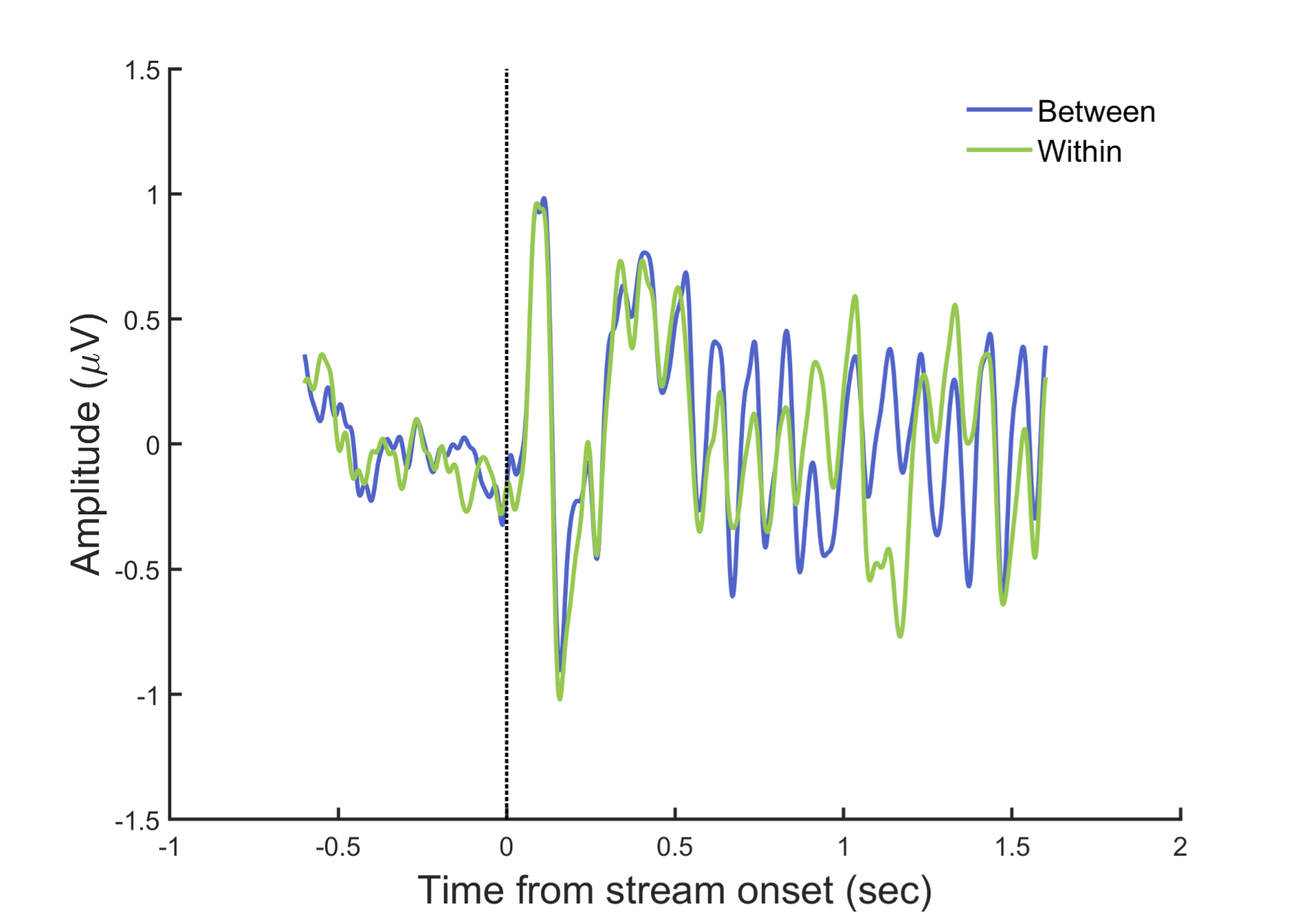
Fig. R1. ERPs aligned to stream onset. EEG signals were filtered between 1–30 Hz, baseline-corrected (-200 to 0 ms before stream onset) and averaged across the electrodes in left parieto-occipital area where 10-Hz alpha power showed attentional modulation effect.
To further inspect the potential differences in the target-related ERP signals between the within- and between-cycle conditions, we plotted the target-aligned waveforms for these experimental conditions. As shown in Fig. R2, a drop of ERP amplitude occurred for both conditions around T2 onset, and the difference between these two conditions was not significant (paired t-test estimated on mean amplitude every 20 ms from 0 to 700 ms relative to T1 onset, p > .05, FDR-corrected).
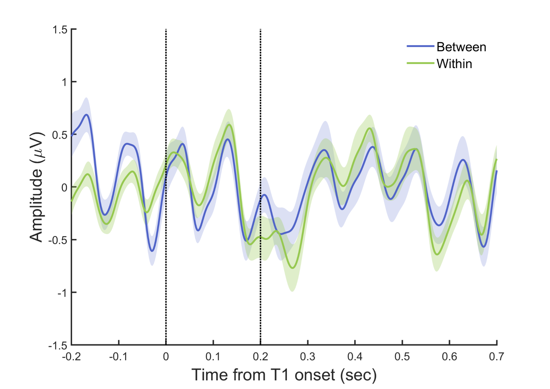
Fig. R2. ERPs aligned to T1 onset. EEG signals were filtered between 1–30 Hz, and baseline-corrected using signals -100 to 0 ms before T1 onset. The two dash lines indicate the onset of T1 and T2, respectively.
Since there is a trend of enhanced ERP response for the between-cycle relative to the within-cycle condition during the period of 0 to 100 ms after T2 onset (paired t-test on mean amplitude, p =.065, uncorrected), we then directly examined whether such post-T2 responses contribute to the behavioral attentional modulation effect and behavior-related neural indices. Crucially, we did not find any significant correlation of such T2-related ERP enhancement with the behavioral modulation index (BMI), or with the reported effects of alpha power and cross-frequency coupling (PAC). Furthermore, after controlling for the T2-related ERP responses, there still remains a significant correlation between the delta-alpha PAC and the BMI (rpartial = .596, p = .019), which is not surprising given that the PAC is calculated based on an 800-ms time window covering more pre-T2 than post-T2 periods (see the response to point #4 for details) rather than around the T2 onset. Taken together, these results clearly suggest that the T2-related ERP responses cannot explain the attentional modulation effect and the observed behavior-related neural indices.
2) The alpha-band increase for T2 is indeed contradictory to the well known inhibitory function of alpha-band in attention. How could a target that is better discriminated elicit stronger inhibitory response? Related to the above point, the observed enhancement in alpha-band power and its coupling to low-frequency oscillation might derive from an enhanced ERP response for T2 target.
Many thanks for the comment. We have briefly discussed this point in the revised manuscript (page 18, line 477).
A widely accepted function of alpha activity in attention is that alpha oscillations suppress irrelevant visual information during spatial selection (Kelly et al., 2006; Thut et al., 2006; Worden et al., 2000). However, it becomes a controversial issue when there exists rhythmic sensory stimulation at alpha-band, just like the situation in the current study where both the visual stream and the contextual auditory rhythm were emitted at 10 Hz. In such a case, alpha-band neural responses at the stimulation frequency can be interpreted as either passively evoked steady-state responses (SSR) or actively synchronized intrinsic brain rhythms. From the former perspective (i.e., the SSR view), an increase in the amplitude or power at the stimulus frequency may indicate an enhanced attentional allocation to the stimulus stream that may result in better target detection (Janson et al., 2014; Keil et al., 2006; Müller & Hübner, 2002). Conversely, the latter view of the inhibitory function of intrinsic alpha oscillations would produce the opposite prediction. In a previous AB study, Janson and colleagues (2014) investigated this issue by separating the stimulus-evoked activity at 12 Hz (using the same power analysis method as ours) from the endogenous alpha oscillations ranging from 10.35 to 11.25 Hz (as indexed by individual alpha frequency, IAF). Interestingly, they found a dissociation between these two alpha-band neural responses, showing that the RSVP frequency power was higher in non-AB trials (T2 detected) than in AB trials (T2 undetected) while the IAF power exhibited the opposite pattern. According to these findings, the currently observed increase in alpha power for the between-cycle condition may reflect more of the stimulus-driven processes related to attentional enhancement. However, we don’t negate the effect of intrinsic alpha oscillations in our study, as the current design is not sufficient to distinguish between these two processes. We have discussed this point in the revised manuscript (page 18, line 477). Also, we have to admit that “alpha power” may not be the most precise term to describe our findings of the stimulus-related results. Thus, we have specified it as “neural responses to first-order rhythms at 10 Hz” and “10-Hz alpha power” in the revised manuscript (see page 12 in the Results section and page 18 in the Discussion section).
As for the contribution of T2-related ERP response to the observed effect of 10 Hz power and cross-frequency coupling, please refer to our response to point #1.
References:
Janson, J., De Vos, M., Thorne, J. D., & Kranczioch, C. (2014). Endogenous and Rapid Serial Visual Presentation-induced Alpha Band Oscillations in the Attentional Blink. Journal of Cognitive Neuroscience, 26(7), 1454–1468. https://doi.org/10.1162/jocn_a_00551
Keil, A., Ihssen, N., & Heim, S. (2006). Early cortical facilitation for emotionally arousing targets during the attentional blink. BMC Biology, 4(1), 23. https://doi.org/10.1186/1741-7007-4-23
Kelly, S. P., Lalor, E. C., Reilly, R. B., & Foxe, J. J. (2006). Increases in Alpha Oscillatory Power Reflect an Active Retinotopic Mechanism for Distracter Suppression During Sustained Visuospatial Attention. Journal of Neurophysiology, 95(6), 3844–3851. https://doi.org/10.1152/jn.01234.2005
Müller, M. M., & Hübner, R. (2002). Can the Spotlight of Attention Be Shaped Like a Doughnut? Evidence From Steady-State Visual Evoked Potentials. Psychological Science, 13(2), 119–124. https://doi.org/10.1111/1467-9280.00422
Thut, G., Nietzel, A., Brandt, S., & Pascual-Leone, A. (2006). Alpha-band electroencephalographic activity over occipital cortex indexes visuospatial attention bias and predicts visual target detection. The Journal of Neuroscience : The Official Journal of the Society for Neuroscience, 26(37), 9494–9502. https://doi.org/10.1523/JNEUROSCI.0875-06.2006
Worden, M. S., Foxe, J. J., Wang, N., & Simpson, G. V. (2000). Anticipatory Biasing of Visuospatial Attention Indexed by Retinotopically Specific α-Bank Electroencephalography Increases over Occipital Cortex. Journal of Neuroscience, 20(6), RC63–RC63. https://doi.org/10.1523/JNEUROSCI.20-06-j0002.2000
3) To support that it is the context-induced entrainment that leads to the modulation in AB effect, the authors could examine pre-T2 response, e.g., alpha-power, and cross-frequency coupling, as well as its relationship to behavioral performance. I think the pre-stimulus response might be more convincing to support the authors' claim.
Many thanks for the insightful suggestion. We have conducted additional analyses.
Following this suggestion, we have examined the 10-Hz alpha power within the time window of -100–0 ms before T2 onset and found stronger activity for the between-cycle condition than for the within-cycle condition. This pre-T2 response is similar to the post-T2 response except that it is more restricted to the left parieto-occipital cluster (CP3, CP5, P3, P5, PO3, PO5, POZ, O1, OZ, t(15) = 2.774, p = .007), which partially overlaps with the cluster that exhibits a delta-alpha coupling effect significantly correlated with the BMI. We have incorporated these findings into the main text (page 12, line 315) and the Fig. 5A of the revised manuscript.
As for the coupling results reported in our manuscript, the coupling index (PAC) was calculated based on the activity during the second and third cycles (i.e., 400 to 1200 ms from stream onset) of the contextual rhythm, most of which covers the pre-T2 period as T2 always appeared in the third cycle for both conditions. Together, these results on pre-T2 10-Hz alpha power and cross-frequency coupling, as well as its relationship to behavioral performance, jointly suggest that the observed modulation effect is caused by the context-induced entrainment rather than being a by-product of post-T2 processing.
4) About the entrainment to rhythmic context and its relation to behavioral modulation index. Previous studies (e.g., Ding et al) have demonstrated the hierarchical temporal structure in speech signals, e.g., emergence of word-level entrainment introduced by language experience. Therefore, it is well expected that imposing a second-order structure on a visual stream would elicit the corresponding steady-state response. I understand that the new part and main focus here are the AB effects. The authors should add more texts explaining how their findings contribute new understandings to the neural mechanism for the intriguing phenomena.
Many thanks for the suggestion. We have provided more discussion in the revised manuscript (page 17, line 447).
We have provided more discussion on this important issue in the revised manuscript (page 17, line 447). In brief, our study demonstrates how cortical tracking of feature-based hierarchical structure reframes the deployment of attentional resources over visual streams. This effect, distinct from the hierarchical entrainment to speech signals (Ding et al., 2016; Gross et al., 2013), does not rely on previously acquired knowledge about the structured information and can be established automatically even when the higher-order structure comes from a task-irrelevant and cross-modal contextual rhythm. On the other hand, our finding sheds fresh light on the adaptive value of the structure-based entrainment effect by expanding its role from rhythmic information (e.g., speech) perception to temporal attention deployment. To our knowledge, few studies have tackled this issue in visual or speech processing.
References:
Ding, N., Melloni, L., Zhang, H., Tian, X., & Poeppel, D. (2016). Cortical tracking of hierarchical linguistic structures in connected speech. Nature Neuroscience, 19(1), 158–164. https://doi.org/10.1038/nn.4186
Gross, J., Hoogenboom, N., Thut, G., Schyns, P., Panzeri, S., Belin, P., & Garrod, S. (2013). Speech Rhythms and Multiplexed Oscillatory Sensory Coding in the Human Brain. PLoS Biol, 11(12). https://doi.org/10.1371/journal.pbio.1001752
Reviewer #2 (Public Review):
In cognitive neuroscience, a large number of studies proposed that neural entrainment, i.e., synchronization of neural activity and low-frequency external rhythms, is a key mechanism for temporal attention. In psychology and especially in vision, attentional blink is the most established paradigm to study temporal attention. Nevertheless, as far as I know, few studies try to link neural entrainment in the cognitive neuroscience literature with attentional blink in the psychology literature. The current study, however, bridges this gap.
The study provides new evidence for the dynamic attending theory using the attentional blink paradigm. Furthermore, it is shown that neural entrainment to the sensory rhythm, measured by EEG, is related to the attentional blink effect. The authors also show that event/chunk boundaries are not enough to modulate the attentional blink effect, and suggest that strict rhythmicity is required to modulate attention in time.
In general, I enjoyed reading the manuscript and only have a few relatively minor concerns.
1) Details about EEG analysis.
. First, each epoch is from -600 ms before the stimulus onset to 1600 ms after the stimulus onset. Therefore, the epoch is 2200 s in duration. However, zero-padding is needed to make the epoch duration 2000 s (for 0.5-Hz resolution). This is confusing. Furthermore, for a more conservative analysis, I recommend to also analyze the response between 400 ms and 1600 ms, to avoid the onset response, and show the results in a supplementary figure. The short duration reduces the frequency resolution but still allows seeing a 2.5-Hz response.
Thanks for the comments. Each epoch was indeed segmented from -600 to 1600 ms relative to the stimulus onset, but in the spectrum analysis, we only used EEG signals from stream onset (i.e., time point 0) to 1600 ms (see the Materials and Methods section) to investigate the oscillatory characteristics of the neural responses purely elicited by rhythmic stimuli. The 1.6-s signals were zero-padded into a 2-s duration to achieve a frequency resolution of 0.5 Hz.
According to the reviewer’s suggestion, we analyzed the EEG signals from 400 ms to 1600 ms relative to stream onset to avoid potential influence of the onset response, and showed the results in Figure 4. Basically, we can still observe spectral peaks at the stimulus frequencies of 2.5, 5 (the harmonic of 2.5 Hz), and 10 Hz for both power and ITPC spectrum. However, the peak magnitudes were much weaker than those of 1.6-s signals especially for 2.5 Hz, and the 2.5-Hz power did not survive the multiple comparisons correction across frequencies (FDR threshold of p < .05), which might be due to the relatively low signal-to-noise ratio for the analysis based on the 1.2-s epochs (only three cycles to estimate the activity at 2.5 Hz). Importantly, we did identify a significant cluster for 2.5 Hz ITPC in the left parieto-occipital region showing a positive correlation with the individuals’ BMI (Fig. R3; CP5, TP7, P5, P7, PO5, PO7, O1; r = .538, p = .016), which is consistent with the findings based on the longer epochs.
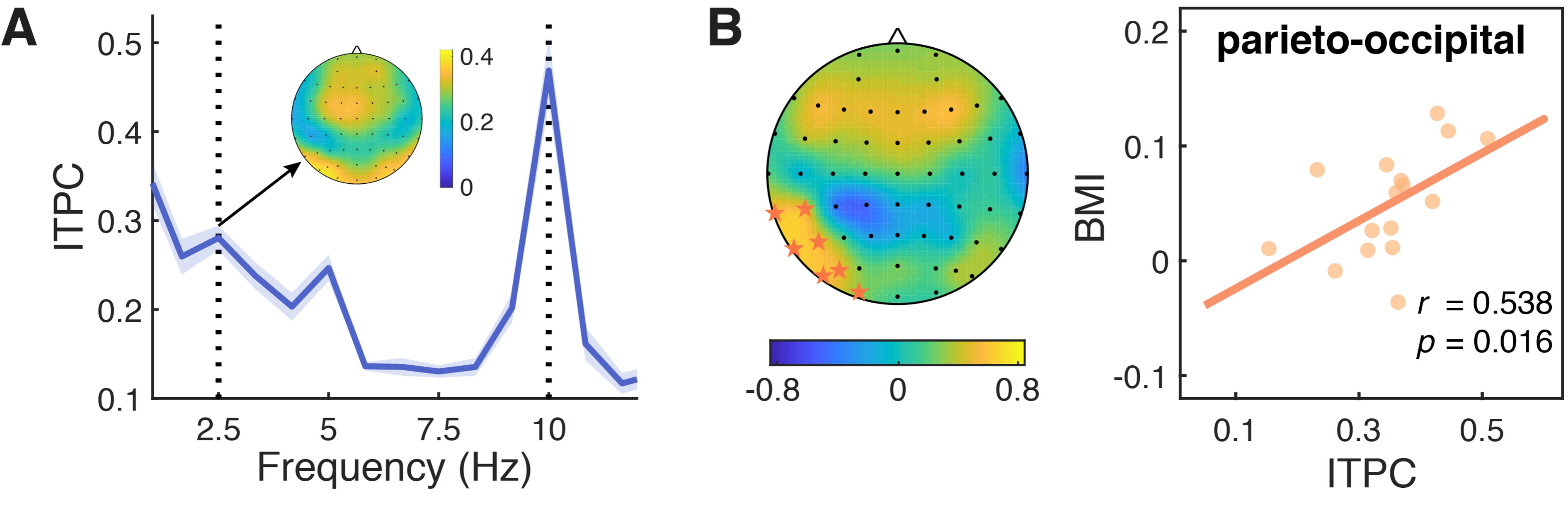
Fig. R3. Neural entrainment to contextual rhythms during the period of 400–1600 ms from stream onset. (A) The spectrum for inter-trial phase coherence (ITPC) of EEG signals from 400 to 1600 ms after the stimulus onset. Shaded areas indicate standard errors of the mean. (B) The 2.5-Hz ITPC was significantly correlated with the behavioral modulation index (BMI) in a parieto-occipital cluster, as indicated by orange stars in the scalp topographic map.
Second, "The preprocessed EEG signals were first corrected by subtracting the average activity of the entire stream for each epoch, and then averaged across trials for each condition, each participant, and each electrode." I have several concerns about this procedure.
(A) What is the entire stream? It's the average over time?
Yes, as for the power spectrum analysis, EEG signals were first demeaned by subtracting the average signals of the entire stream over time from onset to offset (i.e., from 0 to 1600 ms) before further analysis. We performed this procedure following previous studies on the entrainment to visual rhythms (Spaak et al., 2014). We have clarified this point in the “Power analysis” part of the Materials and Methods section (page 25, line 677).
References:
Spaak, E., Lange, F. P. de, & Jensen, O. (2014). Local Entrainment of Alpha Oscillations by Visual Stimuli Causes Cyclic Modulation of Perception. The Journal of Neuroscience, 34(10), 3536–3544. https://doi.org/10.1523/JNEUROSCI.4385-13.2014
(B) I suggest to do the Fourier transform first and average the spectrum over participants and electrodes. Averaging the EEG waveforms require the assumption that all electrodes/participants have the same response phase, which is not necessarily true.
Thanks for the suggestion. In an AB paradigm, the evoked neural responses are sufficiently time-locked to the periodic stimulation, so it is reasonable to quantify power estimate with spectral decomposition performed on trial-averaged EEG signals (i.e., evoked power). Moreover, our results of inter-trial phase coherence (ITPC), which estimated the phase-locking value across trials based on single-trial decomposed phase values, also provided supporting evidence that the EEG waveforms were temporally locked across trials to the 2.5-Hz temporal structure in the context session.
Nevertheless, we also took the reviewer’s suggestion seriously and analyzed the power spectrum on the average of single-trial spectral transforms, i.e., the induced power, which puts emphasis on the intrinsic non-phase-locked activities. In line with the results of evoked power and ITPC, the induced power spectrum in context session also peaked at 2.5 Hz and was significantly stronger than that in baseline session at 2.5 Hz (t(15) = 4.186, p < .001, FDR-corrected with a p value threshold < .001). Importantly, Person correlation analysis also revealed a positive cluster in the left parieto-occipital region, indicating the induced power at 2.5 Hz also had strong relevance with the attentional modulation effect (P7, PO7, PO5, PO3; r = .606, p = .006). We have added these additional findings to the revised manuscript (page 11, line 288; see also Figure 4—figure supplement 1).
2) The sequences are short, only containing 16 items and 4 cycles. Furthermore, the targets are presented in the 2nd or 3rd cycle. I suspect that a stronger effect may be observed if the sequence are longer, since attention may not well entrain to the external stimulus until a few cycles. In the first trial of the experiment, they participant may not have a chance to realize that the task-irrelevant auditory/visual stimulus has a cyclic nature and it is not likely that their attention will entrain to such cycles. As the experiment precedes, they learns that the stimulus is cyclic and may allocate their attention rhythmically. Therefore, I feel that the participants do not just rely on the rhythmic information within a trial but also rely on the stimulus history. Please discuss why short sequences are used and whether it is possible to see buildup of the effect over trials or over cycles within a trial.
Thanks for the comments. Typically, to induce a classic pattern of AB effect, the RSVP stream should contain 3–7 distractors before the first target (T1), with varying lengths of distractors (0–7) between two targets and at least 2 items after the second target (T2). In our study, we created the RSVP streams following these rules, which allowed us to observe the typical AB effect that T2 performance was deteriorated at Lag 2 relative to that at Lag 8. Nevertheless, we agree with the reviewer that longer streams would be better for building up the attentional entrainment effect, as we did observe the attentional modulation effect ramped up as the stream proceeded over cycles, consistent with the reviewer’s speculation. In Experiments 1a (using auditory context) and 2a (using color-defined visual context), we adopted two sets of target positions—an early one where T2 appeared at the 6th or 8th position (in the 2nd cycle) of the visual stream, and a late one where T2 appeared at the 10th or 12th position (in the 3rd cycle) of the visual stream. In the manuscript, we reported T2 performance with all the target positions combined, as no significant interaction was found between the target positions and the experimental conditions (ps. > .1). However, additional analysis demonstrated a trend toward an increase of the attentional modulation effect over cycles, from the early to the late positions. As shown in Fig. R4, the modulation effect went stronger and reached significance for the late positions (for Experiment 1a, t(15) = 2.83, p = .013, Cohen’s d = 0.707; for Experiment 2a, t(15) = 3.656, p = .002, Cohen’s d = 0.914) but showed a weaker trend for the early positions (for Experiment 1a, t(15) = 1.049, p = .311, Cohen’s d = 0.262; for Experiment 2a, t(15) = .606, p = .553, Cohen’s d = 0.152).
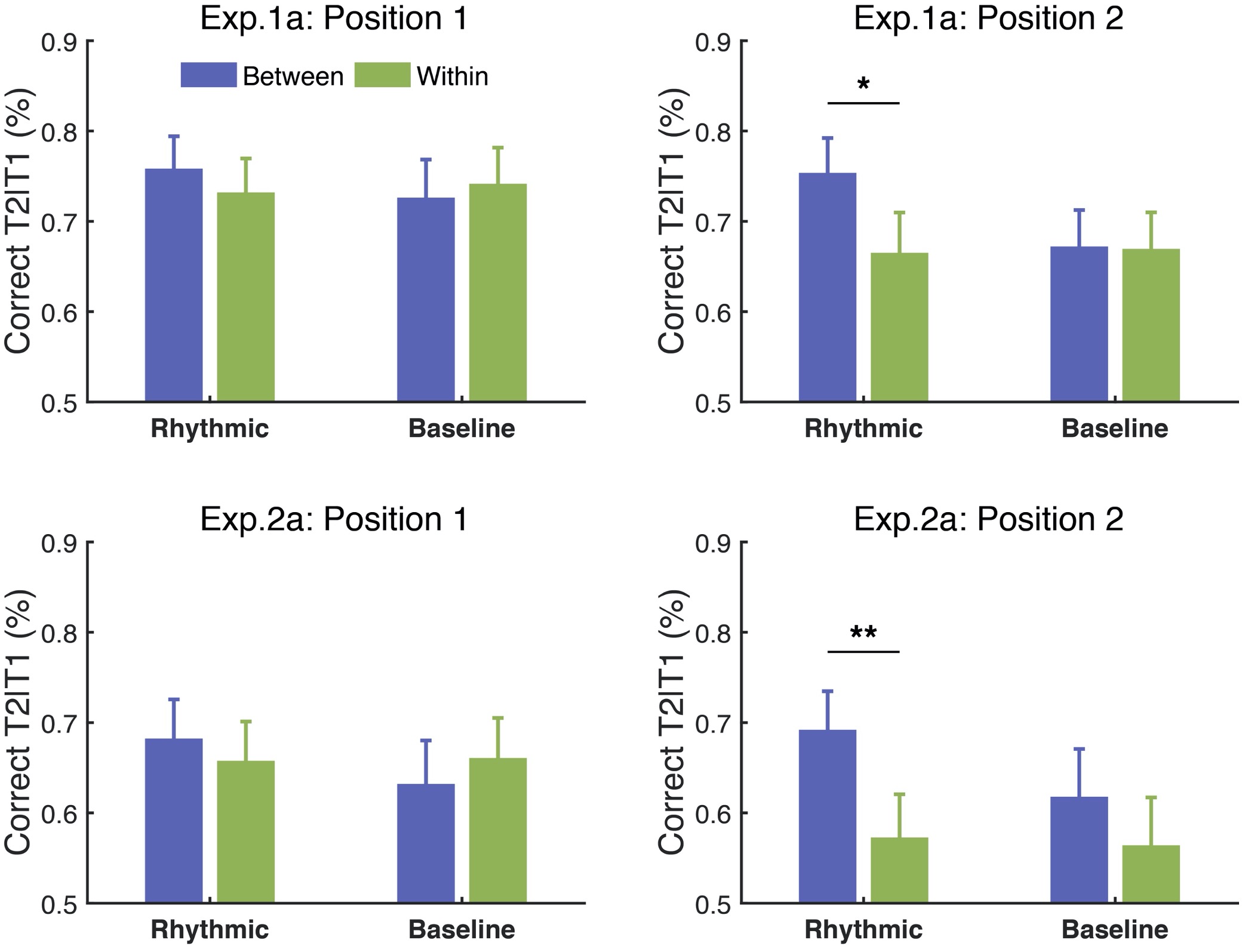
Fig. R4. Attentional modulation effect built up over cycles in Experiments 1a & 2a. Error bars represent 1 SEM; * p<0.05, ** p<0.01.
However, we did not observe an obvious buildup effect across trials in our study. The modulation effect of contextual rhythms seems to be a quick process that the effect is evident in the first quarter of trials in Experiment 1a (for, t(15) = 2.703, p = .016, Cohen’s d = 0.676) and in the second quarter of trials in Experiment 2a (for, t(15) = 2.478, p = .026, Cohen’s d = 0.620.
3) The term "cycle" is used without definition in Results. Please define and mention that it's an abstract term and does not require the stimulus to have "cycles".
Thanks for the suggestion. By its definition, the term “cycle” refers to “an interval of time during which a sequence of a recurring succession of events or phenomena is completed” or “a course or series of events or operations that recur regularly and usually lead back to the starting point” (Merriam-Webster dictionary). In the current study, we stuck to the recurrent and regular nature of “cycle” in general while defined the specific meaning of “cycle” by feature-based periodic changes of the contextual stimuli in each experiment (page 5, line 101; also refer to Procedures in the Materials and Methods section for details). For example, in Experiment 1a, the background tone sequence changed its pitch value from high to low or vice versa isochronously at a rate of 2.5 Hz, thus forming a rhythmic context with structure-based cycles of 400 ms. Note that we did not use the more general term “chunk”, because arbitrary chunks without the regularity of cycles are insufficient to trigger the attentional modulation effect in the current study. Indeed, the effect was eliminated when we replaced the rhythmic cycles with irregular chunks (Experiments 1d & 1e).
4) Entrainment of attention is not necessarily related to neural entrainment to sensory stimulus, and there is considerable debate about whether neural entrainment to sensory stimulus should be called entrainment. Too much emphasis on terminology is of course counterproductive but a short discussion on these issues is probably necessary.
Thanks for the comments. As commonly accepted, entrainment is defined as the alignment of intrinsic neuronal activity to the temporal structure of external rhythmic inputs (Lakatos et al., 2019; Obleser & Kayser, 2019). Here, we are interested in the functional roles of cortical entrainment to the higher-order temporal structure imposed on first-order sensory stimulation, and used the term entrainment to describe the phase-locking neural responses to such hierarchical structure following literature on auditory and visual perception (Brookshire et al., 2017; Doelling & Poeppel, 2015). In our study, the consistent results of power and ITPC have provided strong evidence that neural entrainment at the structure level (2.5 Hz) is significantly correlated with the observed attentional modulation effect. However, this does not mean that the entrainment of attention is necessarily associated with neural entrainment to sensory stimulus in a broader context, as attention may also be guided by predictions based on non-isochronous temporal regularity without requiring stimulus-based oscillatory entrainment (Breska & Deouell, 2017; Morillon et al._2016).
On the other hand, there has been a debate about whether the neural alignment to rhythmic stimulation reflects active entrainment of endogenous oscillatory processes (i.e., induced activity) or a series of passively evoked steady-state responses (Keitel et al., 2019; Notbohm et al., 2016; Zoefel et al., 2018). The latter process is also referred to as “entrainment in a broad sense” by Obleser & Kayser (2019). Given that a presented rhythm always evokes event-related potentials, a better question might be whether the observed alignment reflects the entrainment of endogenous oscillations in addition to evoked steady-state responses. Here we attempted to tackle this issue by measuring the induced power, which emphasizes the intrinsic non-phase-locked activity, in addition to the phase-locked evoked power. Specifically, we quantified these two kinds of activities with the average of single-trial EEG power spectra and the power spectra of trial-averaged EEG signals, respectively, according to Keitel et al. (2019). In addition to the observation of evoked responses to the contextual structure, we also demonstrated an attention-related neural tracking of the higher-order temporal structure based on the induced power at 2.5 Hz (see Figure 4—figure supplement 1), suggesting that the observed attentional modulation effect is at least partially derived from the entrainment of intrinsic oscillatory brain activity. We have briefly discussed this point in the revised manuscript (page 17, line 460).
References:
Breska, A., & Deouell, L. Y. (2017). Neural mechanisms of rhythm-based temporal prediction: Delta phase-locking reflects temporal predictability but not rhythmic entrainment. PLOS Biology, 15(2), e2001665. https://doi.org/10.1371/journal.pbio.2001665
Brookshire, G., Lu, J., Nusbaum, H. C., Goldin-Meadow, S., & Casasanto, D. (2017). Visual cortex entrains to sign language. Proceedings of the National Academy of Sciences, 114(24), 6352–6357. https://doi.org/10.1073/pnas.1620350114
Doelling, K. B., & Poeppel, D. (2015). Cortical entrainment to music and its modulation by expertise. Proceedings of the National Academy of Sciences, 112(45), E6233–E6242. https://doi.org/10.1073/pnas.1508431112
Henry, M. J., Herrmann, B., & Obleser, J. (2014). Entrained neural oscillations in multiple frequency bands comodulate behavior. Proceedings of the National Academy of Sciences, 111(41), 14935–14940. https://doi.org/10.1073/pnas.1408741111
Keitel, C., Keitel, A., Benwell, C. S. Y., Daube, C., Thut, G., & Gross, J. (2019). Stimulus-Driven Brain Rhythms within the Alpha Band: The Attentional-Modulation Conundrum. The Journal of Neuroscience, 39(16), 3119–3129. https://doi.org/10.1523/JNEUROSCI.1633-18.2019
Lakatos, P., Gross, J., & Thut, G. (2019). A New Unifying Account of the Roles of Neuronal Entrainment. Current Biology, 29(18), R890–R905. https://doi.org/10.1016/j.cub.2019.07.075
Morillon, B., Schroeder, C. E., Wyart, V., & Arnal, L. H. (2016). Temporal Prediction in lieu of Periodic Stimulation. Journal of Neuroscience, 36(8), 2342–2347. https://doi.org/10.1523/JNEUROSCI.0836-15.2016
Notbohm, A., Kurths, J., & Herrmann, C. S. (2016). Modification of Brain Oscillations via Rhythmic Light Stimulation Provides Evidence for Entrainment but Not for Superposition of Event-Related Responses. Frontiers in Human Neuroscience, 10. https://doi.org/10.3389/fnhum.2016.00010
Obleser, J., & Kayser, C. (2019). Neural Entrainment and Attentional Selection in the Listening Brain. Trends in Cognitive Sciences, 23(11), 913–926. https://doi.org/10.1016/j.tics.2019.08.004
Zoefel, B., ten Oever, S., & Sack, A. T. (2018). The Involvement of Endogenous Neural Oscillations in the Processing of Rhythmic Input: More Than a Regular Repetition of Evoked Neural Responses. Frontiers in Neuroscience, 12. https://doi.org/10.3389/fnins.2018.00095
Reviewer #3 (Public Review):
The current experiment tests whether the attentional blink is affected by higher-order regularity based on rhythmic organization of contextual features (pitch, color, or motion). The results show that this is indeed the case: the AB effect is smaller when two targets appeared in two adjacent cycles (between-cycle condition) than within the same cycle defined by the background sounds. Experiment 2 shows that this also holds for temporal regularities in the visual domain and Experiment 3 for motion. Additional EEG analysis indicated that the findings obtained can be explained by cortical entrainment to the higher-order contextual structure. Critically feature-based structure of contextual rhythms at 2.5 Hz was correlated with the strength of the attentional modulation effect.
This is an intriguing and exciting finding. It is a clever and innovative approach to reduce the attention blink by presenting a rhythmic higher-order regularity. It is convincing that this pulling out of the AB is driven by cortical entrainment. Overall, the paper is clear, well written and provides adequate control conditions. There is a lot to like about this paper. Yet, there are particular concerns that need to be addressed. Below I outline these concerns:
1) The most pressing concern is the behavioral data. We have to ensure that we are dealing here with a attentional blink. The way the data is presented is not the typical way this is done. Typically in AB designs one see the T2 performance when T1 is ignored relative to when T1 has to be detected. This data is not provided. I am not sure whether this data is collected but if so the reader should see this.
Many thanks for the suggestion. We appreciate the reviewer for his/her thoughtful comments. To demonstrate the AB effect, we did include two T2 lag conditions in our study (Experiments 1a, 1b, 2a, and 2b)—a short-SOA condition where T2 was located at the second lag of T1 (i.e., SOA = 200 ms), and a long-SOA condition where T2 appeared at the 8th lag of T1 (i.e., SOA = 800 ms). In a typical AB effect, T2 performance at short lags is remarkably impaired compared with that at long lags. In our study, we consistently replicated this effect across the experiments, as reported in the Results section of Experiment 1 (page 5, line 106). Overall, the T2 detection accuracy conditioned on correct T1 response was significantly impaired in the short-SOA condition relative to that in the long-SOA condition (mean accuracy > 0.9 for all experiments), during both the context session and the baseline session. More crucially, when looking into the magnitude of the AB effect as measured by (ACClong-SOA - ACCshort-SOA)/ACClong-SOA, we still obtained a significant attentional modulation effect (for Experiment 1a, t(15) = -2.729, p = .016, Cohen’s d = 0.682; for Experiment 2a, t(15) = -4.143, p <.001, Cohen’s d = 1.036) similar to that reflected by the short-SOA condition alone, further confirming that cortical entrainment effectively influences the AB effect.
Although we included both the long- and short-SOA conditions in the current study, we focused on T2 performance in the short-SOA condition rather than along the whole AB curve for the following reasons. Firstly, for the long-SOA conditions, the T2 performance is at ceiling level, making it an inappropriate baseline to probe the attentional modulation effect. We focused on Lag 2 because previous research has identified a robust AB effect around the second lag (Raymond et al., 1992), which provides a reasonable and sensitive baseline to probe the potential modulation effect of the contextual auditory and visual rhythms. Note that instead of using multiple lags, we varied the length of the rhythmic cycles (i.e., a cycle of 300 ms, 400 ms, and 500 ms corresponding to a rhythm frequency of 3.3 Hz, 2.5 Hz, and 2 Hz, respectively, all within the delta band), and showed that the attentional modulation effect could be generalized to these different delta-band rhythmic contexts, regardless of the absolute positions of the targets within the rhythmic cycles.
As to the T1 performance, the overall accuracy was very high, ranging from 0.907 to 0.972, in all of our experiments. The corresponding results have been added to the Results section of the revised manuscript (page 5, line 103). Notably, we did not find T1-T2 trade-offs in most of our experiments, except in Experiment 2a where T1 performance showed a moderate decrease in the between-cycle condition relative to that in the within-cycle condition (mean ± SE: 0.888 ± 0.026 vs. 0.933 ± 0.016, respectively; t(15) = -2.217, p = .043). However, by examining the relationship between the modulation effects (i.e., the difference between the two experimental conditions) on T1 and T2, we did not find any significant correlation (p = .403), suggesting that the better performance for T2 was not simply due to the worse performance in detecting T1.
Finally, previous studies have shown that ignoring T1 would lead to ceiling-level T2 performance (Raymond et al., 1992). Therefore, we did not include such manipulation in the current study, as in that case, it would be almost impossible for us to detect any contextual modulation effect.
References:
Raymond, J. E., Shapiro, K. L., & Arnell, K. M. (1992). Temporary suppression of visual processing in an RSVP task: An attentional blink? Journal of Experimental Psychology: Human Perception and Performance, 18(3), 849–860. https://doi.org/10.1037/0096-1523.18.3.849
2) Also, there is only one lag tested. The ensure that we are dealing here with a true AB I would like to see that more than one lag is tested. In the ideal situation a full AB curve should be presented that includes several lags. This should be done for at least for one of the experiments. It would be informative as we can see how cortical entrainment affects the whole AB curve.
Many thanks for the suggestion. Please refer to our response to the point #1 for “Reviewer #3 (Public Review)”. In short, we did include two T2 lag conditions in our study (Experiments 1a, 1b, 2a and 2b), and the results replicated the typical AB effect. We have clarified this point in the revised manuscript (page 5, line 106).
3) Also, there is no data regarding T1 performance. It is important to show that this the better performance for T2 is not due to worse performance in detecting T1. So also please provide this data.
Many thanks for the suggestion. Please refer to our response to the point #1 or “Reviewer #3 (Public Review)”. We have reported the T1 performance in the revised manuscript (page 5, line 103), and the results didn’t show obvious T1-T2 trade-offs.
4) The authors identify the oscillatory characteristics of EEG signals in response to stimulus rhythms, by examined the FFT spectral peaks by subtracting the mean power of two nearest neighboring frequencies from the power at the stimulus frequency. I am not familiar with this procedure and would like to see some justification for using this technique.
According to previous studies (Nozaradan, 2011; Lenc e al., 2018), the procedure to subtract the average amplitude of neighboring frequency bins can remove unrelated background noise, like muscle activity or eye movement. If there were no EEG oscillatory responses characteristic of stimulus rhythms, the amplitude at a given frequency bin should be similar to the average of its neighbors, and thus no significant peaks could be observed in the subtracted spectrum.
References:
Lenc, T., Keller, P. E., Varlet, M., & Nozaradan, S. (2018). Neural tracking of the musical beat is enhanced by low-frequency sounds. Proceedings of the National Academy of Sciences, 115(32), 8221–8226. https://doi.org/10.1073/pnas.1801421115
Nozaradan, S., Peretz, I., Missal, M., & Mouraux, A. (2011). Tagging the Neuronal Entrainment to Beat and Meter. The Journal of Neuroscience, 31(28), 10234–10240. https://doi.org/10.1523/JNEUROSCI.0411-11.2011
Author Response:
Reviewer #1 (Public Review):
The manuscript by Chakraborty focuses on methods to direct dsDNA to specific cell types within an intact multicellular organism, with the ultimate goal of targeting DNA-based nanodevices, often as biosensors within endosomes and lysosomes. Taking advantage of the endogenous SID-2 dsRNA receptor expressed in C. elegans intestinal cells, the authors show that dsDNA conjugated to dsRNA can be taken into the intestinal endosomal system via feeding and apical endocytosis, while dsDNA alone is not an efficient endocytic cargo from the gut lumen. Since most cells do not express a dsRNA receptor, the authors sought to develop a more generalizable approach. Via phage display screening they identified a novel camelid antibody 9E that recognizes a short specific DNA sequence that can be included at the 3' end of synthesized dsDNAs. The authors then showed that this antibody can direct binding, and in some cases endocytosis, of such DNAs when 9E was expressed as a fusion with transmembrane protein SNB-1. This approach was successful in targeting microinjected dsDNA pan-neuronally when expressed via the snb-1 promoter, and to specific neuronal subsets when expressed via other promoters. Endocytosed dsDNA appeared in puncta moving in neuronal processes, suggesting entry into endosomes. Plasma membrane targeting appeared feasible using 9E fusion to ODR-2.
The major strength of the paper is in the identification and testing of the 9E camelid antibody as part of a generalizable dsDNA targeting system. This aspect of the paper will likely be of wide interest and potentially high impact, since it could be applied in any intact animal system subject to transgene expression. A weakness of the paper is the choice of "nanodevice". It was not clear what utility was present in the DNAs used, such as D38, that made them "devices", aside from their fluorescent tag that allowed tracking their localization.
We used a DNA nanodevice, denoted pHlava-9E, that uses pHrodo as a pH-sensitive dye. pHlava-9E is designed to provide a digital output of compartmentalization i.e., its pH profile is such that even if it is internalized into a mildly acidic vesicle, the pH readout is as high as one would observe with a lysosome. This gives an unambiguous readout of surface-immobilized probe to endocytosed probe.
Another potential weakness is that the delivered DNA is limited to the cell surface or the lumen of endomembrane compartments without access to the cytoplasm or nucleus. In general the data appeared to be of high quality and was well controlled, supporting the authors conclusions.
We completely agree that we cannot target DNA nanodevices to sub-cellular locations such as the cytoplasm or the nucleus with this strategy. However, we do not see this as a “weakness”, but rather, as a limitation of the current capabilities of DNA nanotechnology. It must be mentioned that though fluorescent proteins were first described in 1962, it was 30 years before others targeted them to the endoplasmic reticulum (1992) or the nucleus (1993)(Brini et al., 1993; Kendall et al., 1992). Probe technologies undergo stage-wise improvements/expansions. We have therefore added a small section in the conclusions section outlining the future challenges in sub-cellular targeting of DNA-nanodevices.
Reviewer #2 (Public Review):
The authors demonstrate the tissue-specific and cell-specific targeting of double-stranded DNA (dsDNA) using C. elegans as a model host animal. The authors focused on two distinct tissues and delivery routes: feeding dsDNA to target a class of organelles within intestinal cells, and injecting dsDNA to target presynaptic endocytic structures in neurons. To achieve efficient intestinal targeting, the authors leveraged dsRNA uptake via endogenous intestinal SID-2 receptors by fusing dsRNA to a fluorophore-labeled dsDNA probe. In contrast, neuronal endosome/synaptic vesicle (SV) targeting was achieved by designing a nanobody that specifically binds a short dsDNA motif fused to the fluorophore-labeled dsDNA probe. Combining dsDNA probe injection with nanobody neuronal expression (fused to a neuronal vSNARE to achieve synaptic targeting), the authors demonstrated that the injected dsDNA could be taken up by a variety of distinct neuronal subtypes.
Strengths:
While nanodevices built on dsDNA platforms have been shown to be taken up by scavenger receptors in C. elegans (including previous work from several of these authors), this strategy will not work in many tissue types lacking these receptors. The authors successfully circumvented this limitation using distinct strategies for two cell types in the worm, thereby providing a more general approach for future efforts. The approaches are creative, and the nanobody development in particular allows for endocytic delivery in any cell type. The authors exploited quantitative imaging approaches to examine the subcellular targeting of dsDNA probes in living animals and manipulated endogenous receptors to demonstrate the mechanism of dsRNA-based dsDNA uptake in intestinal cells.
Weaknesses:
To validate successful delivery of a functional nanodevice, one would ideally demonstrate the function of a particular nanodevice in at least one of the examples provided in this work. The authors have successfully used a variety of custom-designed dsDNA probes in living worms in numerous past studies, so this would not be a technical hurdle. In the current study, the reader has no means of assessing whether the dsDNA is intact and functional within its intracellular compartment.
We now demonstrate the use of a functional nanodevice to detect pH profiles of a given microenvironment. This functional nanodevice contains two fluorescent reporter dyes, each attached to one of the strands of a DNA duplex. In order to obtain pH readouts, the device integrity is essential for ratiometric sensing.
Coelomocytes are cells known for their scavenging and degradative lysosomal machinery. Previous studies of the stability of variously structured DNA nanodevices in coelomocytes, have shown that DNA devices based on 38 bp DNA duplexes have a half life of >8 hours in actively scavenging cells such as coelomocytes (Chakraborty et al., 2017; Surana et al., 2013) Given that our sensing in the gut as well as in the neuron are performed in <1 hour post feeding or injection, pHlava-9E is >97% intact.
Another minor weakness is the lack of a quantitative assessment of colocalization in intestinal cells or neurons in an otherwise nicely quantitative study. Since characterization of the targeting described here is an essential part of evaluating the method, a stronger demonstration of colocalization would significantly buttress the authors' claims.
We have now quantified colocalization in each cellular system. Please see Figure R1 below (Figure 1 Supplementary figure 1 and Figure 4 Supplementary figure 2 of the revised manuscript).
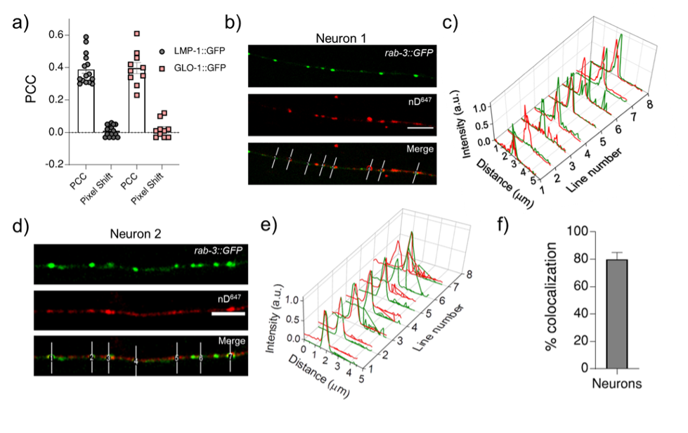
Figure R1: a) Pearson’s correlation coefficient (PCC) calculated for the colocalization between R50D38 (red) and lysosomal markers LMP-1 or GLO-1 (green) in the indicated transgenic worms. b) & d) Representative images of nanodevice nD647 uptake (red) in transgenics expressing both prab-3::gfp::rab-3 (green) and psnb-1:snb-1::9E c - e) Normalized line intensity profiles across the indicated lines in b and d; f) Percentage colocalization of nD647 (red) with RAB3:GFP (green). Error bar represents the standard deviation between two data sets.
While somewhat incomplete, this study represents a step forward in the development of a general targeting approach amenable to nanodevice delivery in animal models.
Summary:
This work is of interest because it increases our understanding of the molecular mechanisms that distinguish subtypes of VIP interneurons in the cerebral cortex and because of the multiple ways in which the authors address the role of Prox1 in regulating synaptic function in these cells.
The authors would like to thank the reviewers for their constructive comments. In response, we would like to clarify a number of issues, as well as outline how we plan to resolve major concerns.
Reviewer #1:
Stachiak and colleagues examine the physiological effects of removing the homeobox TF Prox1 from two subtypes of VIP neurons, defined on the basis of their bipolar vs. multipolar morphology.
The results will be of interest to those in the field, since it is known from prior work that VIP interneurons are not a uniform class and that Prox1 is important for their development.
The authors first show that selective removal of a conditional Prox1 allele using a VIP cre driver line results in a change in paired pulse ratio of presumptive excitatory synaptic responses in multipolar but not bipolar VIP interneurons. The authors then use RNA-seq to identify differentially expressed genes that might contribute and highlight a roughly two-fold reduction in the expression of a transcript encoding a trans-synaptic protein Elfn1 known to contribute to reduced glutamate release in Sst+ interneurons. They then test the potential contribution of Elfn1 to the phenotype by examining whether loss of one allele of Elfn1 globally alters facilitation. They find that facilitation is reduced both by this genetic manipulation and by a pharmacological blockade of presynaptic mGluRs known to interact with Elfn1.
Although the results are interesting, and the authors have worked hard to make their case, the results are not definitive for several reasons:
1) The global reduction of Elfn1 may act cell autonomously, or may have other actions in other cell types. The pharmacological manipulation is less subject to this interpretation, but these results are not as convincing as they could be because the multipolar Prox1 KO cells (Fig. 3 J) still show substantial facilitation comparable, for example to the multipolar control cells in the Elfn1 Het experiment (controls in Fig. 3E). This raises a concern about control for multiple comparisons. Instead of comparing the 6 conditions in Fig 3 with individual t-tests, it may be more appropriate to use ANOVA with posthoc tests controlled for multiple comparisons.
The reviewer’s concerns regarding non-cell-autonomous actions of global Elfn1 KO are well founded. Significant phenotypic alterations have previously been reported, both in the physiology of SST neurons as well in the animals’ behavior (Stachniak, Sylwestrak, Scheiffele, Hall, & Ghosh, 2019; Tomioka et al., 2014). The homozygous Elfn1 KO mouse displays a hyperactive phenotype and epileptic activity after 3 months of age, suggesting generalcortical activity differences exist (Dolan & Mitchell, 2013; Tomioka et al., 2014). Nevertheless, we have not observed such changes in P17-21 Elfn1 heterozygous (Het) animals.
Comparing across different experimental animal lines, for example the multipolar Prox1 KO cells (Fig. 3 J) to the multipolar control cells in the Elfn1 Het experiment (controls in Fig. 3E), is in our view not advisable. There is a plethora of examples in the literature on the effect of mouse strain on even the most basic cellular functions and hence it is always expected that researchers use the correct control animals for their experiments, which in the best case scenario are littermate controls. For these reasons, we would argue that statistical comparisons across mouse lines is not ideal for our study. Elfn1 Het and MSOP data are presented side by side to illustrate that Elfn1 Hets (3C,E) phenocopy the effects of Prox1 deletion (3G,H,I,J). (See also point 3) MSOP effect sizes, however, do show significant differences by ANOVA with Bonferroni post-hoc (normalized change in EPSC amplitude; multipolar prox1 control: +12.1 ± 3.8%, KO: -8.4 ± 4.3%, bipolar prox1 control: -5.2 ± 4.3%, KO: -3.4 ± 4.7%, cell type x genotype interaction, p= 0.02, two way ANOVA).
2) The isolation of glutamatergic currents is not described. Were GABA antagonists present to block GABAergic currents? Especially with the Cs-based internal solutions used, chloride reversal potentials can be somewhat depolarized relative to the -65 mV holding potential. If IPSCs were included it would complicate the analysis.
No, in fact GABA antagonists were not present in these experiments. The holding voltage in our evoked synaptic experiments is -70 mV, which combined with low internal [Cl-] makes it highly unlikely that the excitatory synaptic responses we study are contaminated by GABA-mediated ones, even with a Cs MeSO4-based solution. Nevertheless, we have now performed additional experiments where glutamate receptor blockers were applied in bath and we observe a complete blockade of the synaptic events at -70mV proving that they are AMPA/NMDA receptor mediated. When holding the cell at 0mV with these blockers present, outward currents were clearly visible, suggesting intact GABA-mediated events.
3) The assumption that protein levels of Elfn1 are reduced to half in the het is untested. Synaptic proteins can be controlled at the level of translation and trafficking and WT may not have twice the level of this protein.
We thank reviewer for pointing this out. Our rationale for using the Elfn1 heterozygous animals is rather that transcript levels are reduced by half in heterozygous animals, to match the reduction we found in the mRNA levels of VIP Prox1 KO cells (Fig 2). The principle purpose of the Elfn1 KO experiment was to determine whether the change in Elfn1 transcript levels could be sufficient to explain the synaptic deficit observed in VIP Prox1 KO cells. As the reviewer notes, translational regulation and protein trafficking could ultimately result in even larger changes than 0.5x protein levels at the synapse. This may ultimately explain the observed multipolar/bipolar disparity, which cannot be explained by transcriptional regulation alone (Fig 4).
4) The authors are to be commended for checking whether Elfn1 is regulated by Prox1 only in the multipolar neurons, but unfortunately it is not. The authors speculate that the selective effects reflect a selective distribution of MgluR7, but without additional evidence it is hard to know how likely this explanation is.
Additional experiments are underway to better understand this mechanism.
Reviewer #2:
Stachniak et al., provide an interesting manuscript on the postnatal role of the critical transcription factor, Prox1, which has been shown to be important for many developmental aspects of CGE-derived interneurons. Using a combination of genetic mouse lines, electrophysiology, FACS + RNAseq and molecular imaging, the authors provide evidence that Prox1 is genetically upstream of Elfn1. Moreover, they go on to show that loss of Prox1 in VIP+ cells preferentially impacts those that are multipolar but not the bipolar subgroup characterized by the expression of calretinin. This latter finding is very interesting, as the field is still uncovering how these distinct subgroups emerge but are at a loss of good molecular tools to fully uncover these questions. Overall, this is a great combination of data that uses several different approaches to come to the conclusions presented. I have suggestions that I think would strengthen the manuscript:
1) Can the authors add a supplemental table showing the top 20-30 genes up and down regulated in their Prox1 KOS? This would make these, and additional, data more tenable to readers.
We would be happy to provide supplementary tables with candidate genes at both P8 and P12.
2) It is interesting that loss of Prox1 or Elfn1 leads to phenotypes in multipolar but are not present or mild in bipolar VIP+ cells. The authors test different hypotheses, which they are able to refute and discuss some ideas for how multipolar cells may be more affected by loss of Elfn1, even when the transcript is lost in both multipolar and bipolar after Prox1 deletion. If there is any way to expand upon these ideas experimentally, I believe it would greatly strengthen the manuscript. I understand there is no perfect experiment due to a lack of tools and reagents but if there is a way to develop one of the following ideas or something similar, it would be beneficial:
We thank the reviewer for the note.
a) Would it be possible to co-fill VIPCre labeled cells with biocytin and a retroviral tracer? Then, after the retroviral tracer had time to label a presynaptic cell, assess whether these were preferentially different between bipolar and multipolar cell types, the latter morphology determined by the biocytin fill? This would test whether each VIP+ subtype is differentially targeted.
Although this is a very elegant experiment and we would be excited to do it, we do feel that single-cell rabies virus tracing is technically very challenging and will take many months to troubleshoot before being able to acquire good data. Hence, we think it is beyond the scope of this study.
b) Another biocytin possibility would be to trace filled VIP+ cells and assess whether the dendrites of multipolar and bipolar cells differentially targeted distinct cortical lamina and whether these lamina, in the same section or parallel, were enriched for mGluR7+ afferents.
We thank the reviewer for their suggestion and we are planning on doing these kinds of experiments.
Reviewer #3:
In this work Stachiak and colleagues investigate the role of Prox1 on the development of VIP cells. Prox1 is expressed by the majority of GABAergic derived from the caudal ganglionic eminence (CGE), and as mentioned by the authors, Prox1 has been shown to be necessary for the differentiation, circuit integration, and maintenance of CGE-derived GABAergic cells. Here, Stachiak and colleagues show that removal of Prox1 in VIP cells leads to suppression of synaptic release probability onto cortical multipolar VIP cells in a mechanism dependent on Elfn1. This work is of interest for the field because it increases our understanding of differential synaptic maturation of VIP cells. The results are noteworthy, however the relevance of this manuscript would potentially be increased by addressing the following suggestions:
1) Include histology to show when exactly Prox1 is removed from multipolar and bipolar VIP-expressing cells by using the VIP-Cre mouse driver.
We can address this by performing an in-situ hybridization against Prox1 from P3 onwards (when Cre becomes active).
2) Clarify if the statistical analysis is done using n (number of cells) or N (number of animals). The analysis between control and mutants (both Prox1 and Elfn1) need to be done across animals and not cells.
Statistics for physiology were done across n (number of cells) while statistics for ISH are done across number of slices. We will clarify this point in the text and update the methods.
Regarding the statistics for the ISH, these have been done across n (number of slices) for control versus KO tissue (N = 3 and N = 2 animals, respectively). We will add more animals to this analysis to compare by animal instead, although we do not expect any change in the results.
Regarding the physiology, we would provide a two-pronged answer. We first of all feel that averaging synaptic responses for each animal would hide a good deal of the biological variability in PPR present in different cells (response Fig 1), the characterization of which is integral to the central findings of the paper. Secondly, to perform such analysis asked by the reviewer one would need to obtain recordings from ~10 animals or so per condition for each condition, which, to our knowledge, is something that is not standard when utilizing in vitro electrophysiological recordings from single cells. For example, in these very recent studies that have performed in vitro electrophysiological recordings all the statistics are performed using “n” number of cells and not the average of all the cells recorded per animal collapsed into a single data point. (Udakis, Pedrosa, Chamberlain, Clopath, & Mellor, 2020) https://www.nature.com/articles/s41467-020-18074-8
(Horvath, Piazza, Monteggia, & Kavalali, 2020) https://elifesciences.org/articles/52852
(Haas et al., 2018) https://elifesciences.org/articles/31755
Nevertheless, we have now re-run the analysis grouping the cells and averaging the values we get per animal, since we have obtained our data from many animals. The results are more or less indistinguishable from the ones presented in the original submission, except for on p value that rose to 0.07 from 0.03 due to the lack of the required number of animals. We hope that the new plots and statistics presented herein address the concern put forward by the reviewer.
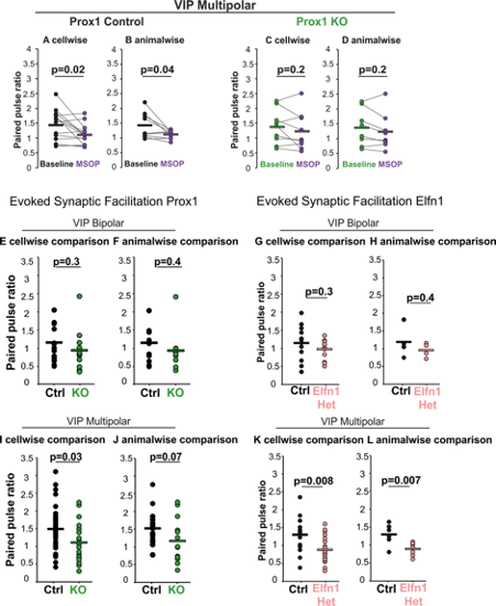
Response Fig 1: A comparison of cell wise versus animal-wise analysis of synaptic physiology. Some cell to cell variability is hidden, and the reduction in numbers impacts the P values.
(A) PPR of multipolar Prox1 Control for 14 cells from 9 animals (n/N=14/9) under baseline conditions and with MSOP, cell-wise comparison p = 0.02 , t = 2.74 and (B) animal-wise comparisons (p = 0.04, t stat = 2.45). Statistics: paired t-test.
(C) PPR of multipolar Prox1 KO cells (n/N=9/8) under baseline conditions and with MSOP, cell-wise comparison p = 0.2, t = 1.33 and (D) animal-wise comparisons (p = 0.2, t stat = 1.56). Statistics: paired t-test. Comparisons for PPR of bipolar Prox1 Control (n/N=8/8) and KO cells (n/N=9/9) did not change.
(E) PPR for Prox1 control (n/N=18/11) and KO (n/N=13/11) bipolar VIP cells, cell-wise comparison p = 0.3, t = 1.1 and (F) animal-wise comparisons (p = 0.4, t stat = 0.93). Statistics: t-test.
(G) PPR of Elfn1 Control (n/N=12/4) and Het (n/N=12/4) bipolar VIP cells, cell-wise comparison p = 0.3, t = 1.06 and (H) animal-wise comparisons (p = 0.4, t stat = 0.93)
(I) PPR of Prox1 control (n/N=33/18) and KO (n/N=19/14) multipolar VIP cells, cell-wise comparison p = 0.03, t = 2.17. and (J) animal-wise comparisons (p = 0.07, t stat = 1.99).
(K) PPR of Elfn1 Control (n/N=14/6) and Het (n/N=20/8) multipolar VIP cells, cell-wise comparison p = 0.008, t = 2.84 and (L) animal-wise comparisons (p = 0.007, t stat = 3.23).
3) Clarify what are the parameters used to identify bipolar vs multipolar VIP cells. VIP cells comprise a wide variety of transcriptomic subtypes, and in the absence of using specific genetic markers for the different VIP subtypes, the authors should either include the reconstructions of all recorded cells or clarify if other methods were used.
We thank the reviewer for this comment. The cell parameter criteria will be amended in the methods: “Cell type was classified as bipolar vs. multipolar based on cell body morphology (ovoid vs. round) and number and orientation of dendritic processes emanating from it (2 or 3 dendrites perpendicular to pia (for bipolar) vs. 3 or more processes in diverse orientations (for multipolar). In addition, the laminar localization of the two populations differs, with multipolar cells found primarily in the upper layer 2, while bipolar cells are found throughout layers 2 and 3. Initial determination of cell classification was made prior to patching fluorescent-labelled cells, but whenever possible this initial assessment was confirmed with post-hoc verification of biocytin filled cells.”
Reference:
Dolan, J., & Mitchell, K. J. (2013). Mutation of Elfn1 in Mice Causes Seizures and Hyperactivity. PLOS ONE, 8(11), e80491. Retrieved from https://doi.org/10.1371/journal.pone.0080491
Haas, K. T., Compans, B., Letellier, M., Bartol, T. M., Grillo-Bosch, D., Sejnowski, T. J., … Hosy, E. (2018). Pre-post synaptic alignment through neuroligin-1 tunes synaptic transmission efficiency. ELife, 7, e31755. https://doi.org/10.7554/eLife.31755
Horvath, P. M., Piazza, M. K., Monteggia, L. M., & Kavalali, E. T. (2020). Spontaneous and evoked neurotransmission are partially segregated at inhibitory synapses. ELife, 9, e52852. https://doi.org/10.7554/eLife.52852
Stachniak, T. J., Sylwestrak, E. L., Scheiffele, P., Hall, B. J., & Ghosh, A. (2019). Elfn1-Induced Constitutive Activation of mGluR7 Determines Frequency-Dependent Recruitment of Somatostatin Interneurons. The Journal of Neuroscience, 39(23), 4461 LP – 4474. https://doi.org/10.1523/JNEUROSCI.2276-18.2019
Tomioka, N. H., Yasuda, H., Miyamoto, H., Hatayama, M., Morimura, N., Matsumoto, Y., … Aruga, J. (2014). Elfn1 recruits presynaptic mGluR7 in trans and its loss results in seizures. Nature Communications. https://doi.org/10.1038/ncomms5501
Udakis, M., Pedrosa, V., Chamberlain, S. E. L., Clopath, C., & Mellor, J. R. (2020). Interneuron-specific plasticity at parvalbumin and somatostatin inhibitory synapses onto CA1 pyramidal neurons shapes hippocampal output. Nature Communications, 11(1), 4395. https://doi.org/10.1038/s41467-020-18074-8
Author Response:
Evaluation Summary:
This manuscript will be of interest to a broad audience of immunologists especially those studying host-pathogen interactions, mucosal immunology, innate immunity and interferons. The study reveals a novel role for neutrophils in the regulation of pathological inflammation during viral infection of the genital mucosa. The main conclusions are well supported by a combination of precise technical approaches including neutrophil-specific gene targeting and antibody-mediated inhibition of selected pathways.
We would like to thank the reviewers for taking the time to review our manuscript, would also like to thank the editors for handling our manuscript. We are grateful for the positive response to our work and the thoughtful suggestions.
Reviewer #1 (Public Review):
Overall this is a well-done study, but some additional controls and experiments are required, as discussed below. The authors have done a considerable amount of work, resulting in quite a lot of negative data, and so should be commended for persistence to eventually identify the link between neutrophils with IL-18, though type I IFN signaling.
Thank you! We appreciate the feedback and suggestions for strengthening the study.
Major Comments:
-A major conclusion of this manuscript is prolonged type I IFN production following vaginal HSV-2 infection, but the data presented herein did not actually demonstrate this. At 2 days post infection, IFN beta was higher (although not significantly) in HSV-2 infection, but much higher in HSV-1 infection compared to uninfected controls. At 5 days post infection the authors show mRNA data, but not protein data. If the authors are relying on prolonged type I IFN production, then they should demonstrate increased IFN beta during HSV-2 infection at multiple days after infection including 5dpi and 7dpi.
We apologize for not including the IFN protein data and have now have provided this information in new Figure 3 and Figure 3 - Supplement 3. This new addition shows measurement of secreted IFNb in vaginal lavages at 4, 5 and 7 d.p.i., as well as total IFNb levels in vaginal tissue at 7 d.p.i..
-Does the CNS viral load or kinetics of viral entry into the CNS differ in mice depleted of neutrophils, IFNAR cKO mice, or mice treated with anti- IL-18? Do neutrophils and/or IL-18 participate at all in neuronal protection from infection?
To maintain the focus of our study on the host factors that contribute specifically to genital disease, we have not included discussion on viral dissemination into the PNS or CNS, especially as viral invasion of
the CNS seems to be an infrequent occurrence during genital herpes in humans. However, we have performed some preliminary exploration of this interesting question, and find that viral invasion of the nervous system is unaltered in the absence of neutrophils. This is in accordance with the lack of antiviral neutrophil activity we have described in the vagina after HSV-2 infection. These preliminary data are provided below as a Reviewer Figure 1. We have not yet begun to investigate whether IL-18 modulates neuroprotection, but agree this is an important question to address in future studies.
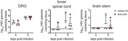
RFigure 1. Viral burden in the nervous system is similar in the presence or absence of neutrophils. Graphs show viral genomes measured by qPCR from the DRG, lower half of of the spinal cord and the brainstem at the indicated days post- infection.
-In Figure 3 the authors show that neutrophil "infection" clusters 2 and 5 express high levels of ISGs. Only 4 of these ISGs are shown in the accompanying figures. Please list which ISGs were increased in neutrophils after both HSV-2 and HSV-1 infection, perhaps in a table. Were there any ISGs specifically higher after HSV-2 infection alone, any after HSV-1 infection alone?
These tables listing differentially-expressed neutrophils ISGs during HSV-1 and HSV-2 have now been provided in new Figure 3 - Supplement 1, with complete lists of DEGs provided as Source Files for the same figure.
-The authors claim that HSV-1 infection recruits non-pathogenic neutrophils compared to the pathogenic neutrophils recruited during HSV-2 infection. Can the authors please discuss if these differences in inflammation or transcriptional differences between the neutrophils in these two different infections could be due to differences in host response to these two viruses rather than differences in inflammation? Please elaborate on why HSV-1 used as opposed to a less inflammatory strain of HSV-2. Furthermore, does HSV-1 infection induce vaginal IL-18 production in a neutrophil-dependent fashion as well?
These are excellent questions, and we have emphasized that differences in host responses against HSV-1 and HSV-2 likely lead to distinct inflammatory milieus that differentially affect neutrophil responses in lines 374-375 and 409-419. We completely agree that differences in neutrophil responses are likely due to distinct host responses against HSV-1 and HSV-2 and apologize for not making that clear. We have previously described some of the other differences in the immunological response against these two viruses (Lee et al, JCI Insight 2020). We would suggest that differences in the host response against these two viruses would naturally result in differences in the local inflammatory milieu, which then modulates neutrophil responses. Whether the transcriptomes of neutrophils beyond the immediate site of infection (outside the vagina) are different between HSV-1 and HSV-2 is currently an open question.
As for why we used HSV-1 instead of a less inflammatory strain of HSV-2, we had originally been interested in trying to model the distinct disease outcomes that have previously been described during HSV-1 vs HSV-2 genital herpes in humans and thought this would be a relevant comparison. We have not yet examined infection with less inflammatory HSV-2 strains, but agree that this is a great idea. We have also not yet examined neutrophil-dependent IL-18 production in the context of HSV-1.
Reviewer #2 (Public Review):
This manuscript will be of interest to a broad audience of immunologists especially those studying host-pathogen interactions, mucosal immunology, innate immunity and interferons. The study reveals a novel role for neutrophils in the regulation of pathological inflammation during viral infection of the genital mucosa. The main conclusions are well supported by a combination of precise technical approaches including neutrophil-specific gene targeting and antibody-mediated inhibition of selected pathways.
In this study by Lebratti, et al the authors examined the impact of neutrophil depletion on disease progression, inflammation and viral control during a genital infection with HSV-2. They find that removal of neutrophils prior to HSV-2 infection resulted in ameliorated disease as assessed by inflammatory score measurements. Importantly, they show that neutrophil depletion had no significant impact on viral burden nor did it affect the recruitment of other immune cells thus suggesting that the observed improvement on inflammation was a direct effect of neutrophils. The role of neutrophils in promoting inflammation appears to be specific to HSV-2 since the authors show that HSV-1 infection resulted in comparable numbers of neutrophils being recruited to the vagina yet HSV-1 infection was less inflammatory. This observation thus suggests that there might be functional differences in neutrophils in the context of HSV-2 versus HSV-1 infection that could underlie the distinct inflammatory outcomes observed in each infection. In ordered to uncover potential mechanisms by which neutrophils affect inflammation the authors examined the contributions of classical neutrophil effector functions such as NETosis (by studying neutrophil-specific PAD4 deficient mice), reactive oxygen species (using mice global defect in NADH oxidase function) and cytokine/phagocytosis (by studying neutrophil-specific STIM-1/STIM-2 deficient mice). The data shown convincingly ruled out a contribution by the neutrophil factors examined. The authors thus performed an unbiased single cell transcriptomic analysis of vaginal tissue during HSV-1 and HSV-2 infection in search for potentially novel factors that differentially regulate inflammation in these two infections. tSNE analysis of the data revealed the presence of three distinct clusters of neutrophils in vaginal tissue in mock infected mice, the same three clusters remained after HSV-1 infection but in response to HSV-2 only two of the clusters remained and showed a sustained interferon signature primarily driven by type I interferons (IFNs). In order to directly interrogate the impact of type I IFN on the regulation of inflammation the authors blocked type I IFN signaling (using anti IFNAR antibodies) at early or late times after infection and showed that late (day 4) IFN signaling was promoting inflammation while early (before infection) IFN was required for antiviral defense as expected. Importantly, the authors examined the impact of neutrophil-intrinsic IFN signaling on HSV-2 infection using neutrophil-specific IFNAR1 knockout mice (IFNAR1 CKO). The genetic ablation of IFNAR1 on neutrophils resulted in reduced inflammation in response to HSV-2 infection but no impact on viral titers; findings that are consistent with observations shown for neutrophil-depleted mice. The use of IFNAR1 CKO mice strongly support the importance of type I IFN signaling on neutrophils as direct regulators of neutrophil inflammatory activity in this model. Since type I IFNs induce the expression of multiple genes that could affect neutrophils and inflammation in various ways the authors set out to identify specific downstream effectors responsible for the observed inflammatory phenotype. This search lead them to IL-18 as possible mediator. They showed that IL-18 levels in the vagina during HSV-2 infection were reduced in neutrophil-depleted mice, in mice with "late" IFNAR blockade and in IFNAR1 CKO mice. Furthermore, they showed that antibody-mediated neutralization of IL-18 ameliorated the inflammatory response of HSV-2 infected mice albeit to a lesser extent that what was seen in IFNAR1 CKO. Altogether, the study presents intriguing data to support a new role for neutrophils as regulators of inflammation during viral infection via an IFN-IL-18 axis.
In aggregate, the data shown support the author's main conclusions, but some of the technical approaches need clarification and in some cases further validation that they are working as intended.
Thank you! We appreciate the enthusiasm for our work as well as the suggestions for improving our study.
1) The use of anti-Ly6G antibodies (clone 1A8) to target neutrophil depletion in mice has been shown to be more specific than anti-Gr1 antibodies (which targets both monocytes and neutrophils) thus anti-Ly6G antibodies are a good technical choice for the study. Neutrophils are notoriously difficult to deplete efficiently in vivo due at least in part to their rapid regeneration in the bone marrow. In order to sustain depletion, previous reports indicate the need for daily injection of antibodies. In the current study the authors report the use of only one, intra-peritoneal injection (500 mg) of 1A8 antibodies and that this single treatment resulted in diminished neutrophil numbers in the vagina at day 5 after viral infection (Fig 1A). Data shown in figure 2B suggests that there are neutrophils present in the vagina of uninfected mice, that there is a significant increase in their numbers at day 2 and that their numbers remain fairly steady from days 2 to 5 after infection. In order to better understand the impact antibody-mediated depletion in this model the authors should have examined the kinetics of depletion from day 0 through 5 in the vaginal tissue after 1A8 injection as compared to the effect of antibodies in the periphery. These additional data sets would allow for a deeper understanding of neutrophil responses in the vagina as compared to what has been published in other models of infection at other mucosal sites.
We agree and apologize for not providing this information in the original submission. Neutrophil depletion kinetics from the vagina have been shown in new Figure 1A, while depletion from the blood is shown in new Figure 1 - Supplement 1.
2) The authors used antibody-mediated blockade as a means to interrogate the impact of type I IFNs and IL-18 in their model. The kinetics of IFNAR blockade were nicely explained and supported by data shown in supplementary figure 4. IFNAR blockade was done by intra-peritoneal delivery of antibodies at one day before infection or at day 4 after infection. When testing the role of IL-18 the authors delivered the blocking antibody intra-vaginally at 3 days post infection. The authors do not provide a rationale for changing delivery method and timing of antibody administration to target IL-18 relative to IFNAR signaling. Since the model presented argues for an upstream role for IFNAR as inducer of IL-18 it is unclear why the time point used to target IL-18 is before the time used for IFNAR.
We thank Reviewer #2 for raising this point and apologize for not providing an explanation for the differences in antibody treatment regimens for modulating IFNAR and IL-18. As the anti-IL-18 mAb is a cytokine neutralizing antibody, we hypothesized that administering the antibody vaginally would help to concentrate the antibody at the relevant site of cytokine production and increase the potency of neutralization. This is in contrast to systemic administration of the anti-IFNAR1 mAb that acts to block signaling in the 'receiving' cell. We expect the anti-IFNAR1 mAb (given in much higher doses) to bind both circulating cells that are recruited to the site of infection as well as cells that are already at the site of infection. Similarly, we started the anti-IL-18 antibody treatment one day earlier to allow a presumably sufficient amount antibody to accumulate in the vagina. Our rationale has been included in the revised manuscript (lines 351-353). We are pleased to report, however, that we have conducted preliminary studies in which mice were treated beginning at 4 d.p.i. rather than 3 d.p.i., and observe similar trends. This data is provided below as Reviewer Figure 3.
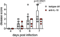
RFigure 3. Mice treated with anti-IL-18 mAb starting at 4 d.p.i. exhibit reduced disease severity. Mice were infected with HSV-2 and treated ivag with 100ug of anti-IL-18 on 4, 5 and 6 d.p.i.. Mice were monitored for disease until 7 d.p.i.. Data was analyzed by repeated measured two-way ANOVA with Geisser-Greenhouse correction and Bonferroni's multiple comparisons test.
3) An open question that remains is the potential mechanism by which IL-18 is acting as effector cytokine of epithelial damage. As acknowledged by the authors the rescue seen in IFNAR1 CKO mice (Fig 5C) is more dramatic that targeting IL-18 (Fig 6D). It is thus very likely that IFNAR signaling on neutrophils is affecting other pathways. It would have been greatly insightful to perform a single cell RNA seq experiment with IFNAR CKO mice as done for WT mice in Fig 3. Such an analysis might would have provided a more thorough understanding of neutrophil-mediated inflammatory pathways that operate outside of classical neutrophil functions.
We agree that the proposed scRNA-seq experiment comparing vaginal cells from IFNAR CKO and WT mice would be very interesting and insightful. Although a bit beyond the scope of the current manuscript, we are currently planning on performing these types of studies to better understand IFN-mediated regulation of inflammatory neutrophil functions.
4) The inflammatory score scale used is nicely described in the methods and it took into consideration external signs of vaginal inflammation by visual observation. It would have been helpful to mention whether the inflammation scoring was done by individuals blinded to the experimental groups.
This is an important point and we apologize for not making this clear. We have now provided this information in the methods section of the revised manuscript (lines 778).
5) The presence of distinct clusters of neutrophils in the scRNA-seq data analysis is a fascinating observation that might suggest more diversity in neutrophils than what is currently appreciated. In this study, the authors do not provide a list of the genes expressed in each cluster within the data shown in the paper. Although the entire data set is deposited and publicly available, having the gene lists within the paper would have been helpful to provide a deeper understanding of the current study.
The heterogeneity of the vaginal neutrophil population after HSV infection is indeed an unexpected finding. To provide a deeper understanding of these transcriptionally distinct clusters, we have now included complete lists of DEGs between the different clusters as Source Files for Figure 3.
Reviewer #3 (Public Review):
This paper examines the role of neutrophils, inflammatory immune cells, in disease caused by genital herpes virus infection. The experiments describe a role for type I interferon stimulation of neutrophils later in the infection that drives inflammation. Blockade of interferon, and to a lesser degree, IL-18 ameliorated disease. This study should be of interest to immunologists and virologists.
This study sought to examine the role of neutrophils in pathology during mucosal HSV-2 infection in a mouse model. The data presented in this manuscript suggest that late or sustained IFN-I signals act on neutrophils to drive inflammation and pathology in genital herpes infection. The authors show that while depletion of neutrophils from mice does not impact viral clearance or recruitment of other immune cells to the infected tissue, it did reduce inflammation in the mucosa and genital skin. Single cell sequencing of immune cells from the infected mucosa revealed increased expression of interferon stimulated genes (ISGs) in neutrophils and myeloid cells in HSV-2 infected mice. Treatment of anti-IFNAR antibodies or neutrophil-specific IFNAR1 conditional knockout mice decreased disease and IL-18 levels. Blocking IL-18 also reduced disease, although these data show that other signals are likely to also be involved. It is interesting that viral titers and anti-viral immune responses were unaffected by IFNAR or IL-18 blockade when this treatment was started 3-4 days after infection, because data shown here (for IFN-I) and by others in published studies (for IFN-I or IL-18) have shown that loss of IFN-I or IL-18 prior to infection is detrimental.
These data are interesting and show pathways (namely IFN-I and IL-18) that could be blocked to limit disease. While this suggests that IL-18 blockade might be an effective treatment for genital inflammation caused by HSV-2 infection, the utility of IL-18 blockade is still unclear, because the magnitude of the effect in this mouse model was less than IFNAR blockade. Additionally, further experiments, such as conditional loss of IL-18 in neutrophils, would be required to better define the role and source(s) of IL-18 that drive disease in this model.
We thank the reviewer for the positive response and agree that additional studies would likely be necessary to fully understand the role of IL-18 during HSV-2 infection.
Reviewer #1:
The Lambowitz group has developed thermostable group II intron reverse transcriptases (TGIRTs) that strand switch and also have trans-lesion activity to provide a much wider view of RNA species analyzed by massively parallel RNA sequencing. In this manuscript they use several improvements to their methodology to identify RNA biotypes in human plasma pooled from several healthy individuals. Additionally, they implicate binding by proteins (RBPs) and nuclease-resistant structures to explain a fraction of the RNAs observed in plasma. Generally I find the study fascinating and argue that the collection of plasma RNAs described is an important tool for those interested in extracellular RNAs. I think the possibility that RNPs are protecting RNA fragments in circulation is exciting and fits with elegant studies of insects and plants where RNAs are protected by this mechanism and are transmitted between species.
I have one major comment for the authors to consider. In my view the use of pooled plasma samples prevented the important opportunity to provide a glimpse on human variation in plasma RNA biotypes. This significantly limits the use of this information to begin addressing RNA biotypes as biomarkers. While I realize that data from multiple individuals represents a significant undertaking and may be beyond the scope of this manuscript, I urge the authors to do two things: (1) downplay the significance of the current study on the development of biomarkers in the current manuscript (e.g., in the abstract and discussion - e.g., "The ability of TGIRT-seq to simultaneously profile a wide variety of RNA biotypes in human plasma, including structured RNAs that are intractable to retroviral RTs, may be advantageous for identifying optimal combinations of coding and non-coding RNA biomarkers for human diseases."). (2) Carry out an analysis in multiple individuals - including racially diverse individuals - very important information will come of this - similar to C. Burge's important study in Nature ~2008 where it was clear that there is important individual variation in alternative splicing decisions - very likely genetically determined. This second suggestion could be added here or constitute a future manuscript.
The identification of biomarkers in human plasma is an important application of this study, as was noted by reviewer 3 -- "Overall, this study provided a robust dataset and expanded picture of RNA biotypes one can detect in human plasma. This is valuable because the findings may have implications in biomarker identification in disease contexts." The present manuscript lays the foundation for such applications, which we have been carrying out in parallel. In one such study in collaboration with Dr. Naoto Ueno (MD Anderson), we used TGIRT-seq to identify combinations of mRNA and non-coding RNA biomarkers in FFPE-tumor slices, PBMCs and plasma from inflammatory breast cancer patients compared to non-IBC breast cancer patients and healthy controls (manuscript in preparation; data presented publicly in seminars), and in another, we explored the potential of using full-length excised intron (FLEXI) RNAs as biomarkers. In the latter study, we identified >8,000 FLEXI RNAs in different human cell lines and tissues and found that they are expressed in a cell-type specific manner, including hundreds of differences between matched tumor and healthy tissues from breast cancer patients and cell lines. A manuscript describing the latter findings was submitted for publication after this one and has been uploaded as a pertinent related manuscript. This new manuscript follows directly from the last sentence of the present manuscript and fully references the BioRxiv preprint currently under review for eLife.
Reviewer #2:
Yao et al used thermostable group II intron reverse transcriptase sequencing (TGIRT-seq) to study apheresis plasma samples. The first interesting discovery is that they had identified a number of mRNA reads with putative binding sites of RNA-binding proteins. A second interesting discovery from this work is the detection of full-length excised intron RNAs.
I have the following comments:
1) One doubt that I have is how representative is apheresis plasma when compared with plasma that one obtains through routine centrifugation of blood. The authors have reported the comparison of apheresis plasma versus a single male plasma in a previous publication. I think that to address this important question, a much increased number of samples would be necessary.
Detailed comparison of plasma prepared by apheresis to that prepared by centrifugation would require a separate large-scale study, preferably by multiple laboratories using different methods to prepare plasma. However, our impression both from our findings and from the literature (Valbonesi et al. 2001, cited in the manuscript) is that apheresis-prepared plasma has very low levels of cellular contamination (required to meet clinical standards) compared to plasma prepared by centrifugation, even with protocols designed to minimize contamination from intact 4 or broken cell (e.g., preparing plasma from freshly drawn blood, centrifugation into a Ficoll cushion to minimize cell breakage, and carefully avoiding contamination from sedimented cells).
We do have additional information about the degree of variation in protein-coding gene transcripts detected by TGIRT-seq in plasma samples prepared by centrifugation from five healthy females controls in our collaborative study with Dr. Naoto Ueno (M.D. Anderson; see above), and we have added it to the manuscript citing a manuscript in preparation with permission from Dr. Ueno (p. 10, beginning line 6 from bottom) as follows:
“The identities and relative abundances of different protein-coding gene transcripts in the apheresis-prepared plasma were broadly similar to those in the previous TGIRT analysis of plasma prepared by Ficoll-cushion sedimentation of blood from a healthy male individual (Qin et al., 2016) (r = 0.62-0.80; Figure 3C) and between high quality plasma samples similarly prepared from five healthy females in a collaborative study with Dr. Naoto Ueno, M.D. Anderson (r = 0.53-0.67; manuscript in preparation).” See Author Response Image below.
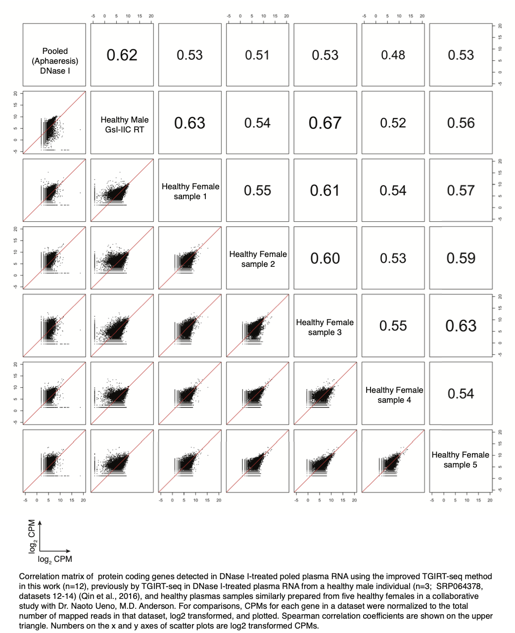
2) For the important conclusion of the presence of binding sites of RNA-binding proteins in a proportion of apheresis plasma mRNA molecules, the authors need to explore whether there is any systemic difference in terms of mapping quality (i.e. mapping quality scores in alignment results) between RBP binding sites and non-RBP binding sites, so that any artifacts of peaks caused by the alignment issues occurring in RNA-seq analysis could be revealed and solved subsequently. Furthermore, it would be prudent to perform immunoprecipitation experiments to confirm this conclusion in at least a proportion of the mRNA.
We have added a figure panel comparing MAPQ scores for reads from peaks containing RBP-binding site to other long RNA reads (Figure 4–figure supplement 2A) and have added further details about the methods used to obtain peaks with high quality reads, including the following (p. 13, beginning line 3 from the bottom).
“After further filtering to remove read alignments with MAPQ <30 (a cutoff that eliminates reads mapping equally well at more than one locus) or ≥5 mismatches from the mapped locus, we were left with 950 high confidence peaks ranging in size from 59 to 1,207 nt with ≥5 high quality read alignments at the peak maximum (Supplementary File).”
3) In Fig. 2D, one can observe that there are clearly more RNA reads in TGIRT-seq located in the 1st exon of ACTB, compared with SMART-seq. Is there any explanation? Will this signal be called as a peak (a potential RBP binding site) in the peak calling analysis (MACS2)? Is ACTB supposed to be bound by a certain RBP?
The higher coverage of the ACTB 5'-exon in the TGIRT-seq datasets reflects in part the more uniform 5' to 3' coverage of mRNA sequences by TGIRT-seq compared to SMART-seq, which is biased for 3'-mRNA sequences that have poly(A) tails (current Figure 3F). The signal in the first exon of ACTB was in fact called as a peak by MACS2 (peak ID#893, Supplementary file), which overlapped an annotated binding site for SERBP1 (see Supplementary File).
4) For Fig 2A, it would be informative for the comparison of RNA yield and RNA size profile among different protocols if the author also added the results of TGIRT-seq.
Figure 3D (previously Figure 2A) shows a bioanalyzer trace of PCR amplified cDNAs obtained by SMART-Seq. These cDNAs correspond to 3' mRNA sequences that have poly(A) tails and are not comparable to the bioanalyzer profiles of plasma RNA (Figure 1–figure supplement 1) or read span distributions in the TGIRT-seq datasets (Figure 1B), which are dominated by sncRNAs. The coverage plots for protein-coding gene transcripts show that TGIRT-seq captures mRNA fragments irrespective of length that span the entire mRNA sequence, whereas SMART-seq is biased for 3' sequences linked to poly(A) (Figure 3F). We also note that coverage plots and mRNAs detected by TGIRT-seq remain similar, even if the plasma RNA is chemically fragmented prior to TGIRT-seq library construction (Figure 3F and Figure 3–figure supplement 2).
5) As shown in Figure 4 C (the track of RBP binding sites), it seems quite pervasive in some gene regions. How many RBP binding sites from public eCLIP-seq results are used for overlapping peaks present in TGIRT-seq of plasma RNA? What percentage of plasma RNA reads have fallen within RBP binding sites? Are those peaks present in TGRIT-seq significantly enriched in RBPs binding regions?
Some of these points are addressed under Reviewer 1-comment #4. Additionally, we noted that 109 RBP-binding sites were searched in the original analysis, and we have now added further analyses for 150 RBPs currently available in ENCODE eCLIP datasets with and without irreproducible discovery rate (IDR) analysis (Figure 6 and Figure 6–figure supplement 1). We have also added a tab to the Supplementary File identifying the 109 and 150 RBPs whose binding sites were searched. The requested statistical analysis has been added in Figure 4–figure supplement 2C. The analysis shows that enrichment of RBP-binding site sequences in the 467 called peaks was statistically significant (p<0.001) (p. 14, para. 3, last sentence).
6) Since there is a considerable portion of TGIRT-seq reads related to simple repeat, one possible reason is likely the high abundance of endogenous repeat-related RNA species in plasma. Nonetheless, have authors studied whether the ligation steps in TGIRT-seq have any biases (e.g. GC content) when analyzing human reference RNAs and spike ins (page 4, paragraph 2)?
We have added a note to the manuscript indicating that although repeat RNAs constitute a high proportion of the called peaks, they do not constitute a similarly high proportion of the total RNA reads (Figure 1C; p. 18, para. 2, first sentence). The TGIRT-seq analysis of human reference RNAs and spike-ins showed that TGIRT-seq recapitulates the relative abundance of human transcripts and spike-in comparably to non-strand-specific TruSeq v2 and better than strand-specific TruSeq v3 (Nottingham et al. RNA 2016). Subsequently, we used miRNA reference sets for detailed analysis of TGIRT-seq biases, including developing a computer algorithm for bias correction based on a random forest regression model that provides insight into different factors that contribute to these biases (Xu et al. Sci. Report. 2019). Overall GC content does not make a significant contribution to TGIRT-seq biases (Figure 9 of Xu et al. Sci. Report, 2017). Instead, biases in TGIRT-seq are largely confined to the first three nucleotides at the 5'-end (due to bias of the thermostable 5' App DNA ligase used for 5' RNA-seq adapter addition) and the 3' nucleotide (due to TGIRT-template switching). These end biases are not expected to significantly impact the quantitation of repeat RNAs.
7) As described in Figure 2 legend, there are 0.25 million deduplicated reads for TGIRT-seq reads assigned to protein-coding genes transcripts which are far less than 2.18 million reads for SMART-seq. The authors need to discuss whether the current protocol of TGIRT-seq would cause potential dropouts in mRNA analysis, compared with SMART-seq?
We have added the following to the manuscript (p. 11, para. 1, line 15).
“The larger number of mRNA reads compared to TGIRT-seq (0.28 million) largely reflects that SMART-seq selectively profiles polyadenylated mRNAs, while TGIRT-seq profiles mRNAs together with other more abundant RNA biotypes. In addition, ultra low input SMART-Seq is not strand-specific, resulting in redundant sense and antisense strand reads (Figure 3–figure supplement 1).”
The manuscript contains the following statement regarding potential drop outs (p. 11, para. 2, line 1).
“A scatter plot comparing the relative abundance of transcripts originating from different genes showed that most of the polyadenylated mRNAs detected in DNase I-treated plasma RNA by ultra low input SMART-Seq were also detected by TGIRT-seq at similar TPM values when normalized for protein-coding gene reads (r=0.61), but with some, mostly lower abundance mRNAs undetected either by TGIRT-seq or SMART-Seq, and with SMART-seq unable to detect non-polyadenylated histone mRNAs, which are relatively abundant in plasma (Figure 3E and Figure 3–figure supplement 1).”
8) While scientific thought-provoking, the practical implication of the current work is still unclear. The authors have suggested that their work might have applications for biomarker development. Is it possible to provide one experimental example in the manuscript?
We addressed the relevance of the manuscript to biomarker identification and noted parallel studies that supports this application in the response to reviewer 1--comment 1. We have also modified the final paragraph of the Discussion (p. 30, para. 2).
“The ability of TGIRT-seq to simultaneously profile a wide variety of RNA biotypes in human plasma, including structured RNAs that are intractable to retroviral RTs, may be advantageous for identifying optimal combinations of coding and non-coding RNA biomarkers that could then be incorporated in target RNA panels for diagnosis and routine monitoring of disease progression and response to treatment. The finding that some mRNAs fragments persist in discrete called peaks suggests a strategy for identifying relatively stable mRNA regions that may be more reliably detected than other more labile regions in targeted liquid biopsies. Finally, we note that in addition to their biological and evolutionary interest, short full-length excised intron RNAs and intron RNA fragments, such as those identified here, may be uniquely well suited to serve as stable RNA biomarkers, whose expression is linked to that of numerous protein-coding genes."
Reviewer #3:
In this work, Yao and colleagues described transcriptome profiling of human plasma from healthy individuals by TGIRT-seq. TGIRT is a thermostable group II intron reverse transcriptase that offers improved fidelity, processivity and strand-displacement activity, as compared to standard retroviral RT, so that it can read through highly structured regions. Similar analysis was performed previously (ref. 20), but this study incorporated several improvements in library preparation including optimization of template switching condition and modified adapters to reduce primer dimer and introduce UMI. In their analysis, the authors detected a variety of structural RNA biotypes, as well as reads from protein-coding mRNAs, although the latter is in low abundance. Compared to SMART-Seq, TGIRT-seq also achieved more uniform read coverage across gene bodies. One novel aspect of this study is the peak analysis of TGIRT-seq reads, which revealed ~900 peaks over background. The authors found that these peaks frequently overlap with RBP binding sites, while others tend to have stable predicted secondary structures, which explains why these regions are protected from degradation in plasma. Overall, this study provided a robust dataset and expanded picture of RNA biotypes one can detect in human plasma. This is valuable because the findings may have implications in biomarker identification in disease contexts. On the other hand, the manuscript, in the current form, is relatively descriptive, and can be improved with a clearer message of specific knowledge that can be extracted from the data.
Specific points:
1) Several aspects of bioinformatics analysis can be clarified in more detail. For example, it is unclear how sequencing errors in UMI affect their de-duplication procedure. This is important for their peak analysis, so it should be explained clearly.
We have added details of the procedure used for de-duplication to the following paragraph in Materials and methods (p. 35, para. 2).
“Deduplication of mapped reads was done by UMI, CIGAR string, and genome coordinates (Quinlan, 2014). To accommodate base-calling and PCR errors and non-templated nucleotides that may have been added to the 3' ends of cDNAs during TGIRT-seq library preparation, one mismatch in the UMI was allowed during deduplication, and fragments with the same CIGAR string, genomic coordinates (chromosome start and end positions), and UMI or UMIs that differed by one nucleotide were collapsed into a single fragment. The counts for each read were readjusted to overcome potential UMI saturation for highly-expressed genes by implementing the algorithm described in (Fu et al., 2011), using sequencing tools (https://github.com/wckdouglas/sequencing_tools ).”
Also, it is not described how exon junction reads (when mapped to the genome) are handled in peak calling, although the authors did perform complementary analysis by mapping reads to the reference transcriptome.
We have added this to first sentence of the paragraph describing peak calling against the transcriptome reference (p. 16, line 4), which now reads as follows:
"Peak calling against the human genome reference sequence might miss RBP-binding sites that are close to or overlap exon junctions, as such reads were treated by MACS2 as long reads that span the intervening intron."
2) Overall, the authors provided convincing data that TGIRT-seq has advantages in detecting a wide range of RNA biotypes, especially structured RNAs, compared to other protocols, but these data are more confirmatory, rather than completely new findings (e.g., compared to ref. 20).
As indicated in the response to Reviewer 1, comment 2, we modified the first paragraph of the Discussion to explicitly describe what is added by the present manuscript compared to Qin et al. RNA 2016 (p. 24, para. 2). Additionally, further analysis in response to the reviewers' comments resulted in the interesting finding that stress granule proteins comprised a high proportion of the RBPs whose binding sites were enriched in plasma RNAs (to our knowledge a completely new finding), consistent with a previously suggested link between RNP granules, EV packing, and RNA export (p. 16, last sentence; data shown in Figure 6 and Figure 6–figure supplement 1). Also highlighted in the Discussion p. 26, last sentence, continuing on p. 27).
3) The peak analysis is more novel. The authors observed that 50% of peaks in long RNAs overlap with eCLIP peaks. However, there is no statistical analysis to show whether this overlap is significant or simply due to the pervasive distribution of eCLIP peaks. In fact, it was reported by the original authors that eCLIP peaks cover 20% of the transcriptome.
We have added statistical analysis, which shows that the enrichment of RBP-binding sites in the 467 called peaks is statistically significant at p<0.001 (p. 14, para. 3, last sentence; Figure 4–Figure supplement 2C), as well as scatter plots identifying proteins whose binding sites were more highly represented in plasma than cellular RNAs or vice versa (p. 16, last two sentences; Figure 6 and Figure 6-figure supplement 1).
Similarly, the authors found that a high proportion of remaining peaks can fold into stable secondary structures, but this claim is not backed up by statistics either.
First, near the beginning of the paragraph describing these findings, we added the following to provide a guide as to what can and can't be concluded by RNAfold (p. 17, line 6 from the bottom).
"To evaluate whether these peaks contained RNAs that could potentially fold into stable secondary structures, we used RNAfold, a tool that is widely used for this purpose with the understanding that the predicted structures remain to be validated and could differ under physiological conditions or due to interactions with proteins."
Second, at the end of the same paragraph, we have added the requested statistics (p. 18, para. 1, last sentence).
"Subject to the caveats above regarding conclusions drawn from RNAfold, simulations using peaks randomly generated from long RNA gene sequences indicated that enrichment of RNAs with more stable secondary structures (lower MFEs) in the called RNA peaks was statistically significant (p≤0.019; Figure 4–figure supplement 2D)."
4) Ranking of RBPs depends on the total number of RBP binding sites detected by eCLIP, which is determined by CLIP library complexity and sequencing depth. This issue should be at least discussed.
We have added scatter plots in Figure 6 and Figure 6–figure supplement 1, which show that the relative abundance of different RBP-binding sites detected in plasma differs markedly from that for cellular RNAs in the eCLIP datasets (both for the 109 RBPs searched initially and for 150 RBPs with or without irreproducible discovery rate (IDR) analysis from the ENCODE web site,) As mentioned in comments above, this analysis identified a number of RBP-binding sites that were substantially enriched in plasma RNAs compared to cellular RNAs or vice versa and led to what we think is the important new finding that plasma RNAs are enriched binding sites for a number of stress granule proteins (Figure 6 and Figure 6–figures supplement 1). We thank the reviewers for this and related comments that led to this additional analysis.
5) Enrichment of RBP binding sites and structured RNA in TGIRT-seq data is certainly consistent with one's expectation. However, the paper can be greatly improved if the authors can make a clearer case of what is new that can be learned, as compared to eCLIP data or other related techniques that purify and sequence RNA fragments crosslinked to proteins. What is the additional, independent evidence to show the predicted secondary structures are real?
Compared to CLIP and related methods, peak calling enables more facile identification of candidate RBPs and putatively structured RNAs for further analysis and may be particularly useful for the vanishingly small amounts of RNA present in plasma and other bodily fluids. New findings resulting from peak calling in the present manuscript include that plasma RNAs are enriched in binding sites for stress granule proteins (see above) and the discovery of a variety of novel RNAs, including the full-length excised intron RNAs first identified here and subsequently studied in cellular RNAs in the Yao et al. pertinent submitted manuscript. We also note that peak calling enables the identification of protein-protected and structured mRNA regions that are relatively stable in plasma and may be more reliably detected in targeted liquid biopsy assays than are more labile mRNA regions (p. 17, para. 1, last sentence; and p. 30, para. 2, beginning on line 5).
6) The authors should probably discuss how alignment errors can potentially affect detection of repetitive regions.
In the Empirical Bayes method that we used for the analysis of repeats, repeat sequences were quantified by aggregate counts irrespective of the genomic locus to which they mapped (Materials and methods, p. 38, para. 2, line 5), which should not be affected by alignment errors.
7) Many figures are IGV screenshots, which can be difficult to follow. Some of them can probably be summarized to deliver the message better.
Some IGV-based figures are crucial for showing key features of the RNAs that are called as peaks (e.g., the predicted secondary structures of the full-length excised intron RNAs and intron RNA fragments). However, in the process of reformatting, we have switched in and added non-IGV main text figures including Figure 2 (microbiome analysis), Figure 3 (TGIRT-seq versus SMART-Seq), Figure 4 (repeats), and Figure 6 (new figure comparing relative abundance of RBP-binding sites in plasma versus cells).
Author Response:
Reviewer #1 (Public Review):
Strengths:
1) The model structure is appropriate for the scientific question.
2) The paper addresses a critical feature of SARS-CoV-2 epidemiology which is its much higher prevalence in Hispanic or Latino and Black populations. In this sense, the paper has the potential to serve as a tool to enhance social justice.
3) Generally speaking, the analysis supports the conclusions.
Other considerations:
1) The clean distinction between susceptibility and exposure models described in the paper is conceptually useful but is unlikely to capture reality. Rather, susceptibility to infection is likely to vary more by age whereas exposure is more likely to vary by ethnic group / race. While age cohort are not explicitly distinguished in the model, the authors would do well to at least vary susceptibility across ethnic groups according to different age cohort structure within these groups. This would allow a more precise estimate of the true effect of variability in exposures. Alternatively, this could be mentioned as a limitation of the the current model.
We agree that this would be an important extension for future work and have indicated this in the Discussion, along with the types of data necessary to fit such models:
“Fourth, due to data availability, we have only considered variability in exposure due to one demographic characteristic; models should ideally strive to also account for the effects of age on susceptibility and exposure within strata of race and ethnicity and other relevant demographics, such as socioeconomic status and occupation \cite{Mulberry2021-tc}. These models could be fit using representative serological studies with detailed cross-tabulated seropositivity estimates.”
2) I appreciated that the authors maintained an agnostic stance on the actual value of HIT (across the population & within ethnic groups) based on the results of their model. If there was available data, then it might be possible to arrive at a slightly more precise estimate by fitting the model to serial incidence data (particularly sorted by ethnic group) over time in NYC & Long Island. First, this would give some sense of R_effective. Second, if successive waves were modeled, then the shift in relative incidence & CI among these groups that is predicted in Figure 3 & Sup fig 8 may be observed in the actual data (this fits anecdotally with what I have seen in several states). Third, it may (or may not) be possible to estimate values of critical model parameters such as epsilon. It would be helpful to mention this as possible future work with the model.
Caveats about the impossibility of truly measuring HIT would still apply (due to new variants, shifting use & effective of NPIs, etc….). However, as is, the estimates of possible values for HIT are so wide as to make the underlying data used to train the model almost irrelevant. This makes the potential to leverage the model for policy decisions more limited.
We have highlighted this important limitation in the Discussion:
“Finally, we have estimated model parameters using a single cross-sectional serosurvey. To improve estimates and the ability to distinguish between model structures, future studies should use longitudinal serosurveys or case data stratified by race and ethnicity and corrected for underreporting; the challenge will be ensuring that such data are systematically collected and made publicly available, which has been a persistent barrier to research efforts \cite{Krieger2020-ss}. Addressing these data barriers will also be key for translating these and similar models into actionable policy proposals on vaccine distribution and non-pharmaceutical interventions.”
3) I think the range of R0 in the figures should be extended to go as as low as 1. Much of the pandemic in the US has been defined by local Re that varies between 0.8 & 1.2 (likely based on shifts in the degree of social distancing). I therefore think lower HIT thresholds should be considered and it would be nice to know how the extent of assortative mixing effects estimates at these lower R_e values.
We agree this would be of interest and have extended the range of R0 values. Figure 1 has been updated accordingly (see below); we also updated the text with new findings: “After fitting the models across a range of $\epsilon$ values, we observed that as $\epsilon$ increases, HITs and epidemic final sizes shifted higher back towards the homogeneous case (Figure \ref{fig:model2}, Figure 1-figure supplement 4); this effect was less pronounced for $R_0$ values close to 1.”
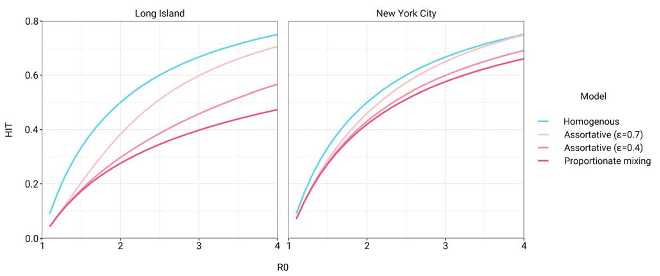
Figure 1: Incorporating assortativity in variable exposure models results in increased HITs across a range of $R_0$ values. Variable exposure models were fitted to NYC and Long Island serosurvey data.
4) line 274: I feel like this point needs to be considered in much more detail, either with a thoughtful discussion or with even with some simple additions to the model. How should these results make policy makers consider race and ethnicity when thinking about the key issues in the field right now such as vaccine allocation, masking, and new variants. I think to achieve the maximal impact, the authors should be very specific about how model results could impact policy making, and how we might lower the tragic discrepancies associated with COVID. If the model / data is insufficient for this purpose at this stage, then what type of data could be gathered that would allow more precise and targeted policy interventions?
We have conducted additional analyses exploring the important suggestion by the reviewers that social distancing could affect these conclusions. The text and figures have been updated accordingly:
“Finally, we assessed how robust these findings were to the impact of social distancing and other non- pharmaceutical interventions (NPIs). We modeled these mitigation measures by scaling the transmission
rate by a factor $\alpha$ beginning when 5\% cumulative incidence in the population was reached. Setting the duration of distancing to be 50 days and allowing $\alpha$ to be either 0.3 or 0.6 (i.e. a 70\% or 40\% reduction in transmission rates, respectively), we assessed how the $R_0$ versus HIT and final epidemic size relationships changed. We found that the $R_0$ versus HIT relationship was similar to in the unmitigated epidemic (Figure 1-figure supplement 5). In contrast, final epidemic sizes depended on the intensity of mitigation measures, though qualitative trends across models (e.g. increased assortativity leads to greater final sizes) remained true (Figure 1-figure supplement 6). To explore this further, we systematically varied $\alpha$ and the duration of NPIs while holding $R_0$ constant at 3. We found again that the HIT was consistent, whereas final epidemic sizes were substantially affected by the choice of mitigation parameters (Figure 1-figure supplement 7); the distribution of cumulative incidence at the point of HIT was also comparable with and without mitigation measures (Figure 2-figure supplement 8). The most stringent NPI intensities did not necessarily lead to the smallest epidemic final sizes, an idea which has been explored in studies analyzing optimal control measures \cite{Neuwirth2020- nb,Handel2007-ee}. Longitudinal changes in incidence rate ratios also were affected by NPIs, but qualitative trends in the ordering of racial and ethnic groups over time remained consistent (Figure 3- figure supplement 3).
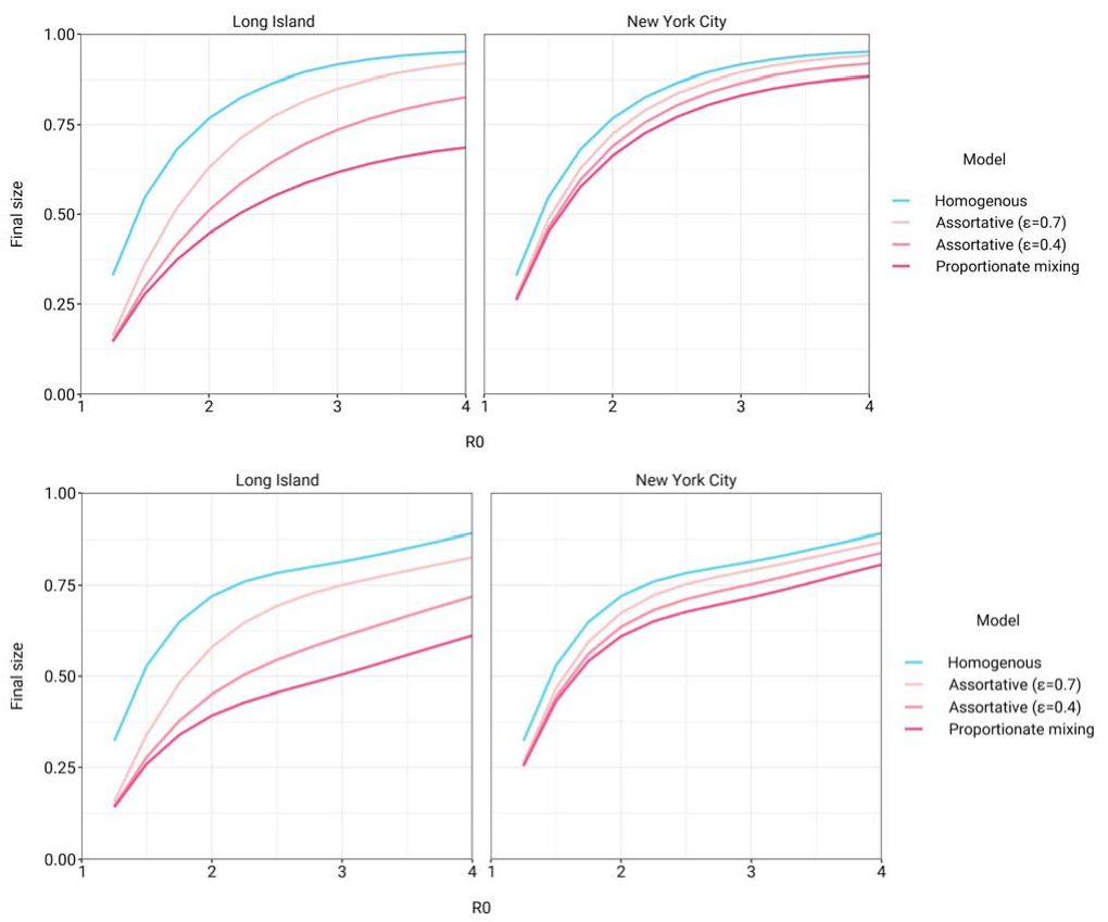
Figure 1-figure supplement 6: Final epidemic sizes versus $R_0$ in variable exposure models with mitigation measures for $\alpha = 0.3$ (top) and $\alpha = 0.6$ (bottom). NPIs were initiated when cumulative incidence reached 5\% in all models and continued for 50 days. Models were fitted to NYC and Long Island serosurvey data.
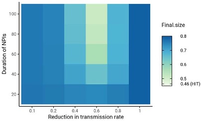
Figure 1-figure supplement 7: Sensitivity analysis on the impact of intensity and duration of NPIs on final epidemic sizes. HIT values for the same mitigation parameters were 46.4 $\pm$ 0.5\% (range). The smallest final size, corresponding to $\alpha = 0.6$ and duration = 100, was 51\%. Census-informed assortativity models were fit to Long Island seroprevalence data. NPIs were initiated when cumulative incidence reached 5\% in all models.
See points 1 and 2 above for examples of additional data required.
Minor issues:
-This is subjective but I found the words "active" and "high activity" to describe increases in contacts per day to be confusing. I would just say more contacts per day. It might help to change "contacts" to "exposure contacts" to emphasize that not all contacts are high risk.
To clarify this, we have replaced instances of “activity level” (and similar) with “total contact rate”, indicating the total number of contacts per unit time per individual; e.g. “The estimated total contact rate ratios indicate higher contacts for minority groups such as Hispanics or Latinos and non-Hispanic Black people, which is in line with studies using cell phone mobility data \cite{Chang2020-in}; however, the magnitudes of the ratios are substantially higher than we expected given the findings from those studies.”
We have also clarified our definition of contacts: “We define contacts to be interactions between individuals that allow for transmission of SARS-CoV-2 with some non-zero probability.”
-The abstract has too much jargon for a generalist journal. I would avoid words like "proportionate mixing" & "assortative" which are very unique to modeling of infectious diseases unless they are first defined in very basic language.
We have revised the abstract to convey these same concepts in a more accessible manner: “A simple model where interactions occur proportionally to contact rates reduced the HIT, but more realistic models of preferential mixing within groups increased the threshold toward the value observed in homogeneous populations.”
-I would cite some of the STD models which have used similar matrices to capture assortative mixing.
We have added a reference in the assortative mixing section to a review of heterogeneous STD models: “Finally, under the \textit{assortative mixing} assumption, we extended this model by partitioning a fraction $\epsilon$ of contacts to be exclusively within-group and distributed the rest of the contacts according to proportionate mixing (with $\delta_{i,j}$ being an indicator variable that is 1 when $i=j$ and 0 otherwise) \cite{Hethcote1996-bf}:”
-Lines 164-5: very good point but I would add that members of ethnic / racial groups are more likely to be essential workers and also to live in multigenerational houses
We have added these helpful examples into the text: “Variable susceptibility to infection across racial and ethnic groups has been less well characterized, and observed disparities in infection rates can already be largely explained by differences in mobility and exposure \cite{Chang2020-in,Zelner2020- mb,Kissler2020-nh}, likely attributable to social factors such as structural racism that have put racial and ethnic minorities in disadvantaged positions (e.g., employment as frontline workers and residence in overcrowded, multigenerational homes) \cite{Henry_Akintobi2020-ld,Thakur2020-tw,Tai2020- ok,Khazanchi2020-xu}.”
-Line 193: "Higher than expected" -> expected by who?
We have clarified this phrase: “The estimated total contact rate ratios indicate higher exposure contacts for minority groups such as Hispanics or Latinos and non-Hispanic Black people, which is in line with studies using cell phone mobility data \cite{Chang2020-in}; however, the magnitudes of the ratios are substantially higher than we expected given the findings from those studies.”
-A limitation that needs further mention is that fact that race & ethnic group, while important, could be sub classified into strata that inform risk even more (such as SES, job type etc….)
We agree and have added this to the Discussion: “Fourth, due to data availability, we have only considered variability in exposure due to one demographic characteristic; models should ideally strive to also account for the effects of age on susceptibility and exposure within strata of race and ethnicity and other relevant demographics, such as socioeconomic status and occupation \cite{Mulberry2021-tc}. These models could be fit using representative serological studies with detailed cross-tabulated seropositivity estimates.”
Reviewer #2 (Public Review):
Overall I think this is a solid and interesting piece that is an important contribution to the literature on COVID-19 disparities, even if it does have some limitations. To this point, most models of SARS-CoV-2 have not included the impact of residential and occupational segregation on differential group-specific covid outcomes. So, the authors are to commended on their rigorous and useful contribution on this valuable topic. I have a few specific questions and concerns, outlined below:
We thank the reviewer for the supportive comments.
1) Does the reliance on serosurvey data collected in public places imply a potential issue with left-censoring, i.e. by not capturing individuals who had died? Can the authors address how survival bias might impact their results? I imagine this could bring the seroprevalence among older people down in a way that could bias their transmission rate estimates.
We have included this important point in the limitations section on potential serosurvey biases: “First, biases in the serosurvey sampling process can substantially affect downstream results; any conclusions drawn depend heavily on the degree to which serosurvey design and post-survey adjustments yield representative samples \cite{Clapham2020-rt}. For instance, because the serosurvey we relied on primarily sampled people at grocery stores, there is both survival bias (cumulative incidence estimates do not account for people who have died) and ascertainment bias (undersampling of at-risk populations that are more likely to self-isolate, such as the elderly) \cite{Rosenberg2020-qw,Accorsi2021-hx}. These biases could affect model estimates if, for instance, the capacity to self-isolate varies by race or ethnicity -- as suggested by associations of neighborhood-level mobility versus demographics \cite{Kishore2020- sy,Kissler2020-nh} -- leading to an overestimate of cumulative incidence and contact rates in whites.”
2) It might be helpful to think in terms of disparities in HITs as well as disparities in contact rates, since the HIT of whites is necessarily dependent on that of Blacks. I'm not really disagreeing with the thrust of what their analysis suggests or even the factual interpretation of it. But I do think it is important to phrase some of the conclusions of the model in ways that are more directly relevant to health equity, i.e. how much infection/vaccination coverage does each group need for members of that group to benefit from indirect protection?
We agree with this important point and indeed this was the goal, in part, of the analyses in Figure 2. We have added additional text to the Discussion highlighting this: “Projecting the epidemic forward indicated that the overall HIT was reached after cumulative incidence had increased disproportionately in minority groups, highlighting the fundamentally inequitable outcome of achieving herd immunity through infection. All of these factors underscore the fact that incorporating heterogeneity in models in a mechanism-free manner can conceal the disparities that underlie changes in epidemic final sizes and HITs. In particular, overall lower HIT and final sizes occur because certain groups suffer not only more infection than average, but more infection than under a homogeneous mixing model; incorporating heterogeneity lowers the HIT but increases it for the highest-risk groups (Figure \ref{fig:hitcomp}).”
For vaccination, see our response to Reviewer #1 point 4.
3) The authors rely on a modified interaction index parameterized directly from their data. It would be helpful if they could explain why they did not rely on any sources of mobility data. Are these just not broken down along the type of race/ethnicity categories that would be necessary to complete this analysis? Integrating some sort of external information on mobility would definitely strengthen the analysis.
This is a great suggestion, but this type of data has generally not been available due to privacy concerns from disaggregating mobility data by race and ethnicity (Kishore et al., 2020). Instead, we modeled NPIs as mentioned in Reviewer #1 point 4, with the caveat that reduction in mobility was assumed to be identical across groups. We added this into the text explicitly as a limitation: “Third, we have assumed the impact of non-pharmaceutical interventions such as stay-at-home policies, closures, and the like to equally affect racial and ethnic groups. Empirical evidence suggests that during periods of lockdown, certain neighborhoods that are disproportionately wealthy and white tend to show greater declines in mobility than others \cite{Kishore2020-sy,Kissler2020-nh}. These simplifying assumptions were made to aid in illustrating the key findings of this model, but for more detailed predictive models, the extent to which activity level differences change could be evaluated using longitudinal contact survey data \cite{Feehan2020-ta}, since granular mobility data are typically not stratified by race and ethnicity due to privacy concerns \cite{Kishore2020-mg}.”
Reviewer #3 (Public Review):
Ma et al investigate the effect of racial and ethnic differences in SARS-CoV-2 infection risk on the herd immunity threshold of each group. Using New York City and Long Island as model settings, they construct a race/ethnicity-structured SEIR model. Differential risk between racial and ethnic groups was parameterized by fitting each model to local seroprevalence data stratified demographically. The authors find that when herd immunity is reached, cumulative incidence varies by more than two fold between ethnic groups, at approximately 75% of Hispanics or Latinos and only 30% of non-Hispanic Whites.
This result was robust to changing assumptions about the source of racial and ethnic disparities. The authors considered differences in disease susceptibility, exposure levels, as well as a census-driven model of assortative mixing. These results show the fundamentally inequitable outcome of achieving herd immunity in an unmitigated epidemic.
The authors have only considered an unmitigated epidemic, without any social distancing, quarantine, masking, or vaccination. If herd immunity is achieved via one of these methods, particularly vaccination, the disparities may be mitigated somewhat but still exist. This will be an important question for epidemiologists and public health officials to consider throughout the vaccine rollout.
We thank the reviewer for the detailed and helpful summary and suggestions.
Author Response
Summary: A major tenet of plant pathogen effector biology has been that effectors from very different pathogens converge on a small number of host targets with central roles in plant immunity. The current work reports that effectors from two very different pathogens, an insect and an oomycete, interact with the same plant protein, SIZ1, previously shown to have a role in plant immunity. Unfortunately, apart from some technical concerns regarding the strength of the data that the effectors and SIZ1 interact in plants, a major limitation of the work is that it is not demonstrated that the effectors alter SIZ1 activity in a meaningful way, nor that SIZ1 is specifically required for action of the effects.
We thank the editor and reviewers for their time to review our manuscript and their helpful and constructive comments. The reviews have helped us focus our attention on additional experiments to test the hypothesis that effectors Mp64 (from an aphid) and CRN83-152 (from an oomycete) indeed alter SIZ1 activity or function. We have revised our manuscript and added the following data:
1) Mp64, but not CRN83-152, stabilizes SIZ1 in planta. (Figure 1 in the revised manuscript).
2) AtSIZ1 ectopic expression in Nicotiana benthamiana triggers cell death from 3-4 days after agroinfiltration. Interestingly CRN83-152_6D10 (a mutant of CRN83-152 that has no cell death activity), but not Mp64, enhances the cell death triggered by AtSIZ1 (Figure 2 in the revised manuscript).
For 1) we have added the following panel to Figure 1 as well as three biological replicates of the stabilisation assays in the Supplementary data (Fig S3):
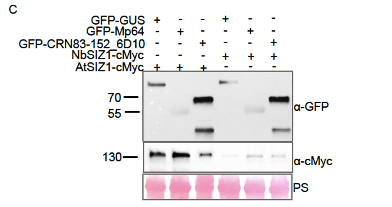
Figure 1 panel C. Stabilisation of SIZ1 by Mp64. Western blot analyses of protein extracts from agroinfiltrated leaves expressing combinations of GFP-GUS, GFP Mp64 and GFP-CRN83_152_6D10 with AtSIZ1-myc or NbSIZ1-myc. Protein size markers are indicated in kD, and equal protein amounts upon transfer is shown upon ponceau staining (PS) of membranes. Blot is representative of three biological replicates , which are all shown in supplementary Fig. S3. The selected panels shown here are cropped from Rep 1 in supplementary Fig. S3.
For 2) we have added the folllowing new figure (Fig. 2 in the revised manuscript):
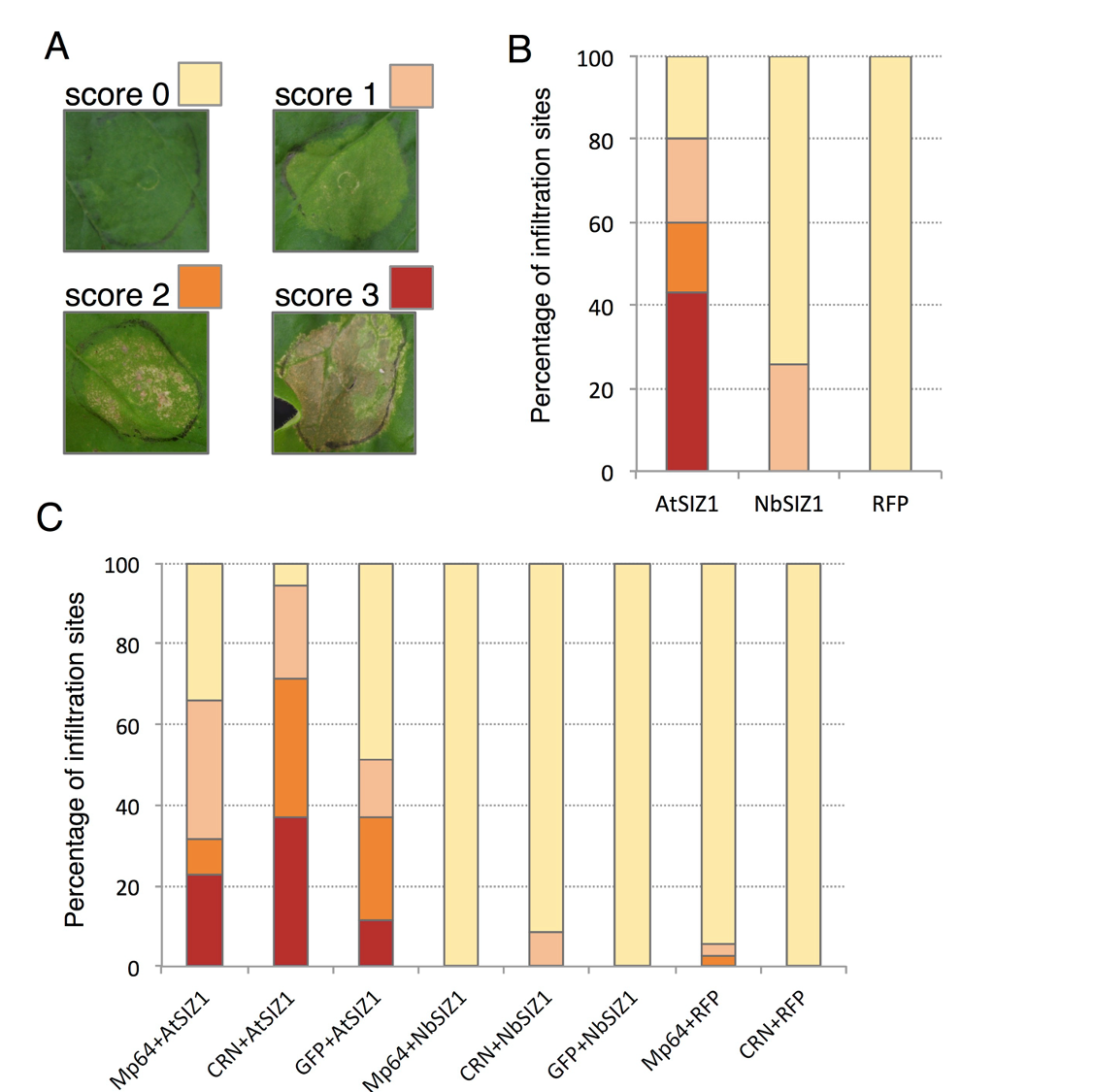
Fig. 2. SIZ1-triggered cell death in N. benthamiana is enhanced by CRN83_152_6D10 but not Mp64. (A) Scoring overview of infiltration sites for SIZ1 triggered cell death. Infiltration site were scored for no symptoms (score 0), chlorosis with localized cell death (score 1), less than 50% of the site showing visible cell death (score 2), more than 50% of the site showing cell death (score 3). (B) Bar graph showing the proportions of infiltration sites showing different levels of cell death upon expression of AtSIZ1, NbSIZ1 (both with a C-terminal RFP tag) and an RFP control. Graph represents data from a combination of 3 biological replicates of 11-12 infiltration sites per experiment (n=35). (C) Bar graph showing the proportions of infiltration sites showing different levels of cell death upon expression of SIZ1 (with C-terminal RFP tag) either alone or in combination with aphid effector Mp64 or Phytophthora capsica effector CRN83_152_6D10 (both effectors with GFP tag), or a GFP control. Graph represent data from a combination of 3 biological replicates of 11-12 infiltration sites per experiment (n=35).
Our new data provide further evidence that SIZ1 function is affected by effectors Mp64 (aphid) and CRN83-152 (oomycete), and that SIZ1 likely is a vital virulence target. Our latest results also provide further support for distinct effector activities towards SIZ1 and its variants in other species. SIZ1 is a key immune regulator to biotic stresses (aphids, oomycetes, bacteria and nematodes), on which distinct virulence strategies seem to converge. The mechanism(s) underlying the stabilisation of SIZ1 by Mp64 is yet unclear. However, we hypothesize that increased stability of SIZ1, which functions as an E3 SUMO ligase, leads to increased SUMOylation activity towards its substrates. We surmise that SIZ1 complex formation with other key regulators of plant immunity may underpin these changes. Whether the cell death, triggered by AtSIZ1 upon transient expression in Nicotiana benthamiana, is linked to E3 SUMO ligase activity remains to be investigated. Expression of AtSIZ1 in a plant species other than Arabidopsis may lead to mistargeting of substrates, and subsequent activation of cell death. Dissecting the mechanistic basis of SIZ1 targeting by distinct pathogens and pests will be an important next step in addressing these hypotheses towards understanding plant immunity.
Reviewer #1:
In this manuscript, the authors suggest that SIZ1, an E3 SUMO ligase, is the target of both an aphid effector (Mp64 form M. persicae) and an oomycete effector (CRN83_152 from Phytophthora capsica), based on interaction between SIZ1 and the two effectors in yeast, co-IP from plant cells and colocalization in the nucleus of plant cells. To support their proposal, the authors investigate the effects of SIZ1 inactivation on resistance to aphids and oomycetes in Arabidopsis and N. benthamiana. Surprisingly, resistance is enhanced, which would suggest that the two effectors increase SIZ1 activity.
Unfortunately, not only do we not learn how the effectors might alter SIZ1 activity, there is also no formal demonstration that the effects of the effectors are mediated by SIZ1, such as investigating the effects of Mp64 overexpression in a siz1 mutant. We note, however, that even this experiment might not be entirely conclusive, since SIZ1 is known to regulate many processes, including immunity. Specifically, siz1 mutants present autoimmune phenotype, and general activation of immunity might be sufficient to attenuate the enhanced aphid susceptibility seen in Mp64 overexpressers.
To demonstrate unambiguously that SIZ1 is a bona fide target of Mp64 and CRN83_152 would require assays that demonstrate either enhanced SIZ1 accumulation or altered SIZ1 activity in the presence of Mp64 and CRN83_152.
The enhanced resistance upon knock-down/out of SIZ1 suggests pathogen and pest susceptibility requires SIZ1. We hypothesize that the effectors either enhance SIZ1 activity or that the effectors alter SIZ1 specificity towards substrates rather than enzyme activity itself. To investigate how effectors coopt SIZ1 function would require a comprehensive set of approaches and will be part of our future work. While we agree that this aspect requires further investigation, we think the proposed experiments go beyond the scope of this study.
After receiving reviewer comments, including on the quality of Figure 1, which shows western blots of co-immunoprecipitation experiments, we re-analyzed independent replicates of effector-SIZ1 coexpression/ co-immunoprecipitation experiments. The reviewer rightly pointed out that in the presence of Mp64, SIZ1 protein levels increase when compared to samples in which either the vector control or CRN83-152_6D10 are co-infiltrated. Through carefully designed experiments, we can now affirm that Mp64 co-expression leads to increased SIZ1 protein levels (Figure 1C and Supplementary Figure S3, revised manuscript). Our results offer both an explanation of different SIZ1 levels in the input samples (original submission, Figure 1A/B) as well as tantalizing new clues to the nature of distinct effector activities.
Besides, we were able to confirm a previous preliminary finding not included in the original submission that ectopic expression of AtSIZ1 in Nicotiana benthamiana triggers cell death (3/4 days after infiltration) and that CRN83-152_6D10 (which itself does not trigger cell death) enhances this phenotype.
We have considered overexpression of Mp64 in the siz1 mutant, but share the view that the outcome of such experiments will be far from conclusive.
In summary, we have added new data that further support that SIZ1 is a bonafide target of Mp64 and CRN83-152 (i.e. increased accumulation of SIZ1 in the presence of Mp64, and enhanced SIZ cell death activation in the presence of CRN83-152_6D10).
Reviewer #2:
The study provides evidence that an aphid effector Mp64 and a Phytophthora capsici effector CRN83_152 can both interact with the SIZ1 E3 SUMO-ligase. The authors further show that overexpression of Mp64 in Arabidopsis can enhance susceptibility to aphids and that a loss-of-function mutation in Arabidopsis SIZ1 or silencing of SIZ1 in N. benthamiana plants lead to increased resistance to aphids and P. capsici. On siz1 plants the aphids show altered feeding patterns on phloem, suggestive of increased phloem resistance. While the finding is potentially interesting, the experiments are preliminary and the main conclusions are not supported by the data.
Specific comments:
The suggestion that SIZ1 is a virulence target is an overstatement. Preferable would be knockouts of effector genes in the aphid or oomycete, but even with transgenic overexpression approaches, there are no direct data that the biological function of the effectors requires SIZ1. For example, is SIZ1 required for the enhanced susceptibility to aphid infestation seen when Mp64 is overexpressed? Or does overexpression of SIZ1 enhance Mp64-mediated susceptibility?
What do the effectors do to SIZ1? Do they alter SUMO-ligase activity? Or are perhaps the effectors SUMOylated by SIZ1, changing effector activity?
We agree that having effector gene knock-outs in aphids and oomycetes would be ideal for dissecting effector mediated targeting of SIZ1. Unfortunately, there is no gene knock-out system established in Myzus persicae (our aphid of interest), and CAS9 mediated knock-out of genes in Phytophthora capsici has not been successful in our lab as yet, despite published reports. Moreover, repeated attempts to silence Mp64, other effector and non-effector coding genes, in aphids (both in planta and in vitro) have not been successful thus far, in our hands. As detailed in our response to Reviewer 1, we considered the use of transgenic approaches not appropriate as data interpretation would become muddied by the strong immunity phenotype seen in the siz1-2 mutant.
As stated before, we hypothesize that the effectors either enhance SIZ1 activity or alter SIZ1 substrate specificity. Mp64-induced accumulation of SIZ1 could form the basis of an increase in overall SIZ1 activity. This hypothesis, however, requires testing. The same applies to the enhanced SIZ1 cell death activation in the presence of CRN83-152_6D10.
Whilst our new data support our hypothesis that effectors Mp64 and CRN83-152 affect SIZ1 function, how exactly these effectors trigger susceptibility, requires significant work. Given the substantial effort needed and the research questions involved, we argue that findings emanating from such experiments warrant standalone publication.
While stable transgenic Mp64 overexpressing lines in Arabidopsis showed increased susceptibility to aphids, transient overexpression of Mp64 in N. benthamiana plants did not affect P. capsici susceptibility. The authors conclude that while the aphid and P. capsici effectors both target SIZ1, their activities are distinct. However, not only is it difficult to compare transient expression experiments in N. benthamiana with stable transgenic Arabidopsis plants, but without knowing whether Mp64 has the same effects on SIZ1 in both systems, to claim a difference in activities remains speculative.
We agree that we cannot compare effector activities between different plant species. We carefully considered every statement regarding results obtained on SIZ1 in Arabidopsis and Nicotiana benthamiana. We can, however, compare activities of the two effectors when expressed side by side in the same plant species. In our original submission, we show that expression of CRN83 152 but not Mp64 in Nicotiana benthamiana enhances susceptibility to Phytophthora capsici. In our revised manuscript, we present new data showing distinct effector activities towards SIZ1 with regards to 1) enhanced SIZ1 stability and 2) enhanced SIZ1 triggered cell death. These findings raise questions as to how enhanced SIZ1 stability and cell death activation is relevant to immunity. We aim to address these critical questions by addressing the mechanistic basis of effector-SIZ1 interactions.
The authors emphasize that the increased resistance to aphids and P. capsici in siz1 mutants or SIZ1 silenced plants are independent of SA. This seems to contradict the evidence from the NahG experiments. In Fig. 5B, the effects of siz1 are suppressed by NahG, indicating that the resistance seen in siz1 plants is completely dependent on SA. In Fig 5A, the effects of siz1 are not completely suppressed by NahG, but greatly attenuated. It has been shown before that SIZ1 acts only partly through SNC1, and the results from the double mutant analyses might simply indicate redundancy, also for the combinations with eds1 and pad4 mutants.
We emphasized that siz1-2 increased resistance to aphids is independent of SA, which is supported by our data (Figure 5A). Still, we did not conclude that the same applies to increased resistance to Phytophthora capsici (Figure 5B). In contrast, the siz1-2 enhanced resistance to P. capsici appears entirely dependent on SA levels, with the level of infection on the siz1-2/NahG mutants even slightly higher than on the NahG line and Col-0 plants. We exercise caution in the interpretation of this data given the significant impact SA signalling appears to have on Phytophthora capsici infection.
The reviewer commented on the potential for functional redundancy in the siz1-2 double mutants. Unfortunately, we are unsure what redundancy s/he is referring to. SNC1, EDS1, and PAD4 all are components required for immunity, and their removal from the immune signalling network (using the mutations in the lines we used here) impairs immunity to various plant pathogens. The siz1-2 snc1-11, siz1-2 eds1-2, and siz1-2 pad4-1 double mutants have similar levels of susceptibility to the bacterial pathogen Pseudomonas syringae when compared to the corresponding snc1-11, eds1-2 and pad4-1 controls (at 22oC). These previous observations indicate that siz1 enhanced resistance is dependent on these signalling components (Hammoudi et al., 2018, Plos Genetics).
In contrast to this, we observed a strong siz1 enhanced resistance phenotype in the absence of snc1- 11, eds1 2 and pad4-1. Notably, the siz1-2 snc1-11 mutant does not appear immuno-compromised when compared to siz1-2 in fecundity assays, indicating that the siz1-2 phenotype is independent of SNC1. In our view, these data suggest that signalling components/pathways other than those mediated by SNC1, EDS1, and PAD4 are involved. We consider this to be an exciting finding as our data points to an as of yet unknown SIZ1-dependent signalling pathway that governs immunity to aphids.
How do NahG or Mp64 overexpression affect aphid phloem ingestion? Is it the opposite of the behavior on siz1 mutants?
We have not performed further EPG experiments on additional transgenic lines used in the aphid assay. These experiments are quite challenging and time consuming. Moreover, accommodating an experimental set-up that allows us to compare multiple lines at the same time is not straightforward. Considering that NahG did not affect aphid performance (Figure 5A), we do not expect to see an effect on phloem ingestion.
Author Response
1) Please comment on why many of the June samples failed to provide sufficient sequence information, especially since not all of them had low yields (supp table 2 and supp figure 5).
An extended paragraph about experimental intricacies of our study has been added to the Discussion. It has also been also slightly restructured to give a better and wider overview of how future freshwater monitoring studies using nanopore sequencing can be improved (page 18, lines 343-359).
We wish to highlight that all three MinION sequencing runs here analysed feature substantially higher data throughput than that of any other recent environmental 16S rRNA sequencing study with nanopore technology, as recently reviewed by Latorre-Pérez et al. (Biology Methods and Protocols 2020, doi:10.1093/biomethods/bpaa016). One of this work's sequencing runs has resulted in lower read numbers for water samples collected in June 2018 (~0.7 Million), in comparison to the ones collected in April and August 2018 (~2.1 and ~5.5 Million, respectively). While log-scale variabilities between MinION flow cell throughput have been widely reported for both 16S and shotgun metagenomics approaches (e.g. see Latorre-Pérez et al.), the count of barcode-specific 16S reads is nevertheless expected to be correlated with the barcode-specific amount of input DNA within a given sequencing run. As displayed in Supplementary Figure 7b, we see a positive, possibly logarithmic trend between the DNA concentration after 16S rDNA amplification and number of reads obtained. With few exceptions (April-6, April-9.1 and Apri-9.2), we find that sample pooling with original 16S rDNA concentrations of ≳4 ng/µl also results in the surpassing of the here-set (conservative) minimum read threshold of 37,000 for further analyses. Conversely, all June samples that failed to reach 37,000 reads did not pass the input concentration of 4 ng/µl, despite our attempt to balance their quantity during multiplexing.
We reason that such skews in the final barcode-specific read distribution would mainly arise from small concentration measurement errors, which undergo subsequent amplification during the upscaling with comparably large sample volume pipetting. While this can be compensated for by high overall flow cell throughput (e.g. see August-2, August-9.1, August-9.2), we think that future studies with much higher barcode numbers can circumvent this challenge by leveraging an exciting software solution: real-time selective sequencing via “Read Until”, as developed by Loose et al. (Nature Methods 2016, doi:10.1038/nmeth.3930). In the envisaged framework, incoming 16S read signals would be in situ screened for the sample-barcode which in our workflow is PCR-added to both the 5' and 3' end of each amplicon. Overrepresented barcodes would then be counterbalanced by targeted voltage inversion and pore "rejection" of such reads, until an even balance is reached. Lately, such methods have been computationally optimised, both through the usage of GPUs (Payne et al., bioRxiv 2020, https://doi.org/10.1101/2020.02.03.926956) and raw electrical signals (Kovaka et al., bioRxiv 2020, https://doi.org/10.1101/2020.02.03.931923).
2) It would be helpful if the authors could mention the amount (or proportion) of their sequenced 16S amplicons that provided species-level identification, since this is one of the advantages of nanopore sequencing.
We wish to emphasize that we intentionally refrained from reporting the proportion of 16S rRNA reads that could be classified at species level, since we are wary of any automated species level assignments even if the full-length 16S rRNA gene is being sequenced. While we list the reasons for this below, we appreciate the interest in the theoretical proportion of reads at species level assignment. We therefore re-analyzed our dataset, and now also provide the ratio of reads that could be classified at species level using Minimap2 (pages 16-17, lines 308-314).
To this end, we classified reads at species level if the species entry of the respective SILVA v.132 taxonomic ID was either not empty, or neither uncultured bacterium nor metagenome. Therefore, many unspecified classifications such as uncultured species of some bacterial genus are counted as species-level classifications, rendering our approach lenient towards a higher ratio of species level classifications. Still, the species level classification ratios remain low, on average at 16.2 % across all included river samples (genus-level: 65.6 %, family level: 76.6 %). The mock community, on the other hand, had a much higher species classification rate (>80 % in all three replicates), which is expected for a well-defined, well-referenced and divergent composition of only eight bacterial taxa, and thus re-validates our overall classification workflow.
On a theoretical level, we mainly refrain from automated across-the-board species level assignments because: (1) many species might differ by very few nucleotide differences within the 16S amplicon; distinguishing these from nanopore sequencing errors (here ~8 %) remains challenging (2) reference databases are incomplete and biased with respect to species level resolution, especially regarding certain environmental contexts; it is likely that species assignments would be guided by references available from more thoroughly studied niches than freshwater
Other recent studies have also shown that across-the-board species-level classification is not yet feasible with 16S nanopore sequencing, for example in comparison with Illumina data (Acharya et al., Scientific Reports 2019, doi:10.25405/data.ncl.9693533) which showed that “more reliable information can be obtained at genus and family level”, or in comparison with longer 16S-ITS-23S amplicons (Cusco et al., F1000Research 2019, doi: 10.12688/f1000research.16817.2), which “remarkably improved the taxonomy assignment at the species level”.
3) It is not entirely clear how the authors define their core microbiome. Are they reporting mainly the most abundant taxa (dominant core microbiome), and would this change if you look at a taxonomic rank below the family level? How does the core compare, for example, with other studies of this same river?
The here-presented core microbiome indeed represents the most abundant taxa, with relatively consistent profiles between samples. We used hierarchical clustering (Figure 4a, C2 and C4) on the bacterial family level, together with relative abundance to identify candidate taxa. Filtering these for median abundance > 0.1% across all samples resulted in 27 core microbiome families. To clarify this for the reader, we have added a new paragraph to the Material and Methods (section 2.7; page 29, lines 653-658).
We have also performed the same analysis on the bacterial genus level and now display the top 27 most abundant genera (median abundance > 0.2%), together with their corresponding families and hierarchical clustering analysis in a new Supplementary Figure 4. Overall, high robustness is observed with respect to the families of the core microbiome: out of the top 16 core families (Figure 4b), only the NS11-12 marine group family is not represented by the top 27 most abundant genera (Supplementary Figure 4b). We reason that this is likely because its corresponding genera are composed of relatively poorly resolved references of uncultured bacteria, which could thus not be further classified.
To the best of our knowledge, there are only two other reports that feature metagenomic data of the River Cam and its wastewater influx sources (Rowe et al., Water Science & Technology 2016, doi:10.2166/wst.2015.634; Rowe et al., Journal of Antimicrobial Chemotherapy 2017, doi:10.1093/jac/dkx017). While both of these primarily focus on the diversity and abundance of antimicrobial resistance genes using Illumina shotgun sequencing, they only provide limited taxonomic resolution on the river's core microbiome. Nonetheless, Rowe et al. (2016) specifically highlighted Sphingobium as the most abundant genus in a source location of the river (Ashwell, Hertfordshire). This genus belongs to the family of Sphingomonadaceae, which is also among the five most dominant families identified in our dataset. It thus forms part of what we define as the core microbiome of the River Cam (Figure 4b), and we have therefore highlighted this consistency in our manuscript's Discussion (page 17, lines 316-319).
4) Please consider revising the amount of information in some of the figures (such as figure 2 and figure 3). The resulting images are tiny, the legends become lengthy and the overall impact is reduced. Consider splitting these or moving some information to the supplements.
To follow this advice, we have split Figure 2 into two less compact figures. We have moved more detailed analyses of our classification tool benchmark to the supplement (now Supplementary Figure 1). Supplementary Figure 1 notably also contains a new summary of the systematic computational performance measurements of each classification tool (see minor suggestions).
Moreover, we here suggest that the original Figure 3 may be divided into two figures: one to visualise the sequencing output, data downsampling and distribution of the most abundant families (now Figure 3), and the other featuring the clustering of bacterial families and associated core microbiome (now Figure 4). We think that both the data summary and clustering/core microbiome analyses are of particular interest to the reader, and that they should be kept as part of the main analyses rather than the supplement – however, we are certainly happy to discuss alternative ideas with the reviewers and editors.
5) Given that the authors claim to provide a simple, fast and optimized workflow it would be good to mention how this workflow differs or provides faster and better analysis than previous work using amplicon sequencing with a MinION sequencer.
Data throughput, sequencing error rates and flow cell stability have seen rapid improvements since the commercial release of MinION in 2015. In consequence, bioinformatics community standards regarding raw data processing and integration steps are still lacking, as illustrated by a thorough recent benchmark of fast5 to fastq format "basecalling" methods (Wick et al., Genome Biology 2019, doi: 10.1186/s13059-019-1727-y).
Early on during our analyses, we noticed that a plethora of bespoke pipelines have been reported in recent 16S environmental surveys using MinION (e.g. Kerkhof et al., Microbiome 2017, 10.1186/s40168-017-0336-9; Cusco et al., F1000 Research 2018, 10.12688/f1000research.16817.2; Acharya et al., Scientific Reports 2019, 10.1038/s41598-019-51997-x; Nygaard et al., Scientific Reports 2020, doi: 10.1038/s41598-020-59771-0). This underlines a need for more unified bioinformatics standards of (full-length) 16S amplicon data treatment, while similar benchmarks exist for short-read 16S metagenomics approaches, as well as for nanopore shotgun sequencing (e.g. Ye et al., Cell 2019, doi: 10.1016/j.cell.2019.07.010; Latorre-Pérez et al., Scientific Reports 2020, doi:10.1038/s41598-020-70491-3).
By adding a thorough speed and memory usage summary (new Supplementary Figure 1b), in addition to our (mis)classification performance tests based on both mock and complex microbial community analyses, we provide the reader with a broad overview of existing options. While the widely used Kraken 2 and Centrifuge methods provide exceptional speed, we find that this comes with a noticeable tradeoff in taxonomic assignment accuracy. We reason that Minimap2 alignments provide a solid compromise between speed and classification performance, with the MAPseq software offering a viable alternative should memory usage limitation apply to users.
We intend to extend this benchmarking process to future tools, and to update it on our GitHub page (https://github.com/d-j-k/puntseq). This page notably also hosts a range of easy-to-use scripts for employing downstream 16S analysis and visualization approaches, including ordination, clustering and alignment tests.
The revised Discussion now emphasises the specific advancements of our study with respect to freshwater analysis and more general standardisation of nanopore 16S sequencing, also in contrast to previous amplicon nanopore sequencing approaches in which only one or two bioinformatics workflows were tested (page 16, lines 297-306).
They also mention that nanopore sequencing is an "inexpensive, easily adaptable and scalable framework" The term "inexpensive" doesn't seem appropriate since it is relative. In addition, they should also discuss that although it is technically convenient in some aspects compared to other sequencers, there are still protocol steps that need certain reagents and equipment that is similar or the same to those needed for other sequencing platforms. Common bottlenecks such as DNA extraction methods, sample preservation and the presence of inhibitory compounds should be mentioned.
We agree with the reviewers that “inexpensive” is indeed a relative term, which needs further clarification. We therefore now state that this approach is “cost-effective” and discuss future developments such as the 96-sample barcoding kits and Flongle flow cells for small-scale water diagnostics applications, which will arguably render lower per-sample analysis costs in the future (page 18, lines 361-365).
Other investigators (e.g. Boykin et al., Genes 2019, doi:10.3390/genes10090632; Acharya et al., Water Technology 2020, doi:10.1016/j.watres.2020.116112) have recently shown that the full application of DNA extraction and in-field nanopore sequencing can be achieved at comparably low expense: Boykin et al. studied cassava plant pathogens using barcoded nanopore shotgun sequencing, and estimated costs of ~45 USD per sample, while we calculate ~100 USD per sample in this study. Acharya et al. undertook in situ water monitoring between Birtley, UK and Addis Ababa, Ethiopia, estimated ~75-150 USD per sample and purchased all necessary equipment for ~10,000 GBP – again, we think that this lies roughly within a similar range as our (local) study's total cost of ~3,670 GBP (Supplementary Table 6).
The revised manuscript now mentions the possibility of increasing sequencing yield by improving DNA extraction methods, by taking sample storage and potential inhibitory compounds into account in the planning phase (page 18, lines 348-352).
Minor points:
-Please include a reference to the statement saying that the river Cam is notorious for the "infections such as leptospirosis".
There are indeed several media reports that link leptospirosis risk to the local River Cam (e.g. https://www.cambridge-news.co.uk/news/cambridge-news/weils-disease-river-cam-leptosirosis-14919008 or https://www.bbc.com/news/uk-england-cambridgeshire-29060018). As we, however, did not find a scientific source for this information, we have slightly adjusted the statement in our manuscript from referring to Cambridge to instead referring to the entire United Kingdom. Accordingly, we now cite two reports from Public Health England (PHE) about serial leptospirosis prevalence in the United Kingdom (page 13, lines 226-227).
-Please check figure 7 for consistency across panels, such as shading in violet and labels on the figures that do not seem to correspond with what is stated in the legend. Please mention what the numbers correspond to in outer ring. Check legend, where it says genes is probably genus.
Thank you for pointing this out. We have revised (now labelled) Figure 8 and removed all inconsistencies between the panels. The legend has also been updated, which now includes a description of the number labelling of the tree, and a clearer differentiation between the colour coding of the tree nodes and the background highlighting of individual nanopore reads.
-Page 6. There is a "data not shown" comment in the text: "Benchmarking of the classification tools on one aquatic sample further confirmed Minimap2's reliable performance in a complex bacterial community, although other tools such as SPINGO (Allard, Ryan, Jeffery, & Claesson, 2015), MAPseq (Matias Rodrigues, Schmidt, Tackmann, & von Mering, 2017), or IDTAXA (Murali et al., 2018) also produced highly concordant results despite variations in speed and memory usage (data not shown)." There appears to be no good reason that this data is not shown. In case the speed and memory usage was not recorded, is advisable to rerun the analysis and quantify these variables, rather than mentioning them and not reporting them. Otherwise, provide an explanation for not showing the data please.
This is a valid point, and we agree with the reviewers that it is worth properly following up on this initial observation. To this end, our revised manuscript now entails a systematic characterisation of the twelve tools' runtime and memory usage performance. This has been added as Supplementary Figure 1b and under the new Materials and Methods section 2.2.4 (page 26, lines 556-562), while the corresponding results and their implications are discussed on page 16, lines 301-306. Particularly with respect to the runtime measurements, it is worth noting that these can differ by several orders of magnitude between the classifiers, thus providing an additional clarification on our choice of the - relatively fast - Minimap2 alignments.
-In Figure 4, it would be important to calculate if the family PCA component contribution differences in time are differentially significant. In Panel B, depicted is the most evident variance difference but what about other taxa which might not be very abundant but differ in time? One can use the fitFeatureModel function from the metagenomeSeq R library and a P-adjusted threshold value of 0.05, to validate abundance differences in addition to your analysis.
To assess if the PC component contribution of Figure 5 (previously Figure 4) significantly differed between the three time points, we have applied non-parametric tests to all season-grouped samples except for the mock community controls. We first applied Kruskal-Wallis H-test for independent samples, followed by post-hoc comparisons using two-sided Mann-Whitney U rank tests.
The Kruskal-Wallis test established a significant difference in PC component contributions between the three time points (p = 0.0049), with most of the difference stemming from divergence between April and August samples according to the post-hoc tests (p = 0.0022). The June sampled seemed to be more similar to the August ones (p = 0.66) than to the ones from April (p = 0.11), recapitulating the results of our hierarchical clustering analysis (Figure 4a).
We have followed the reviewers' advice and applied a complementary approach, using the fitFeatureModel of metagenomeSeq to fit a zero-inflated log-normal mixture model of each bacterial taxon against the time points. As only three independent variables can be accounted for by the model (including the intercept), we have chosen to investigate the difference between the spring (April) and summer (June, August) months to capture the previously identified difference between these months. At a nominal P-value threshold of 0.05, this analysis identifies seven families to significantly differ in their relative composition between spring and summer, namely Cyanobiaceae, Armatimonadaceae, Listeriaceae, Carnobacteriaceae, Azospirillaceae, Cryomorphaceae, and Microbacteriaceae. Three out of these seven families were also detected by the PCA component analysis (Carnobacteriacaea, Azospirillaceae, Microbacteriaceae) and two more (Listeriacaea, Armatimonadaceae) occured in the top 15 % of that analysis (out of 357 families).
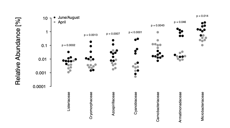
This approach represents a useful validation of our principal component analysis' capture of likely seasonal divergence, but moreover allows for a direct assessment of differential bacterial composition across time points. We have therefore integrated the analysis into our manuscript (page 10, lines 184-186; Materials and Methods section 2.6, page 29, lines 641-647) – thank you again for this suggestion.
-Page 12-13. In the paragraph: "Using multiple sequence alignments between nanopore reads and pathogenic species references, we further resolved the phylogenies of three common potentially pathogenic genera occurring in our river samples, Legionella, Salmonella and Pseudomonas (Figure 7a-c; Material and Methods). While Legionella and Salmonella diversities presented negligible levels of known harmful species, a cluster of reads in downstream sections indicated a low abundance of the opportunistic, environmental pathogen Pseudomonas aeruginosa (Figure 7c). We also found significant variations in relative abundances of the Leptospira genus, which was recently described to be enriched in wastewater effluents in Germany (Numberger et al., 2019) (Figure 7d)."
Here it is important to mention the relative abundance in the sample. While no further experiments are needed, the authors should mention and discuss that the presence of DNA from pathogens in the sample has to be confirmed by other microbiology methodologies, to validate if there are viable organisms. Definitively, it is a big warning finding pathogen's DNA but also, since it is characterized only at genus level, further investigation using whole metagenome shotgun sequencing or isolation, would be important.
We agree that further microbiological assays, particularly target-specific species isolation and culturing, would be essential to validate the presence of living pathogenic bacteria. Accordingly, our revised Discussion now contains a paragraph that encourages such experiments as part of the design of future studies (with a fully-equipped laboratory infrastructure); page 17, 338-341.
-Page 15: "This might help to establish this family as an indicator for bacterial community shifts along with water temperature fluctuations."
Temperature might not be the main factor for the shift. There could be other factors that were not measured that could contribute to this shift. There are several parameters that are not measured and are related to water quality (COD, organic matter, PO4, etc).
We agree that this was a simplified statement, given our currently limited number of samples, and have therefore slightly expanded on this point (page 17, lines 323-325). It is indeed possible that differential Carnobacteriaceae abundances between the time point measurements may have arisen not as a consequence of temperature fluctuations (alone), but instead as a consequence of the observed hydrochemical changes like e.g. Ca2+, Mg2+, HCO3- (Figure 6b-c) or possible even water flow speed reductions (Supplementary Figure 6d).
-"A number of experimental intricacies should be addressed towards future nanopore freshwater sequencing studies with our approach, mostly by scrutinising water DNA extraction yields, PCR biases and molar imbalances in barcode multiplexing (Figure 3a; Supplementary Figure 5)."
Here you could elaborate more on the challenges, as mentioned previously.
We realise that we had not discussed the challenges in enough detail, and the Discussion now contains a substantially more detailed description of these intricacies (page 18, lines 343-359).
Reviewer #1:
Summary:
In this paper, the authors utilize CRISPR-Cas9 to generate two different DMD cell lines. The first is a DMD human myoblast cell line that lacks exon 52 within the dystrophin gene. The second is a DMD patient cell line that is missing miRNA binding sites within the regulatory regions of the utrophin gene, resulting in increased utrophin expression. Then, the authors proceeded to test antisense oligonucleotides and utrophin up-regulators in these cell lines.
Overall opinion (expanded in more detail below).
The paper suffers from the following weaknesses:
1) The protocol used to generate the myoblast cell lines is rather inefficient and is not new.
2) Many of the data figures are of low quality and are missing proper controls (detailed in points 5,7,10, 12, 13,14)
Detailed critiques:
1) The title needs to be changed. The method used by the authors is inefficient. The title should instead focus on the two cell lines generated.
We appreciate the reviewer’s comments: thanks to them, we have realized the focus of the manuscript should be in the new models we described and less in the methodology used to create them.
Originally, we wanted to share the problems we faced when applying new CRISPR/Cas9 edition techniques to myoblasts: our conversations with other researchers in the field confirmed that many were having similar problems. However, the reviewer is right in the fact that there are many ways around this problem. We do describe ours and we are working in a new version of the manuscript with additional data to characterize our new models further and where the method used to create them, although included, is not the main focus of the manuscript. In this new version we will change the title accordingly.
2) Line 104: The authors declare that the efficiency of CRISPR/Cas9 is currently too low to provide therapeutic benefit for DMD in vivo. There are lots of papers that show efficient recovery of dystrophin in small and large animals following CRISPR/Cas9 therapy. The authors should cite them properly.
Thank you for your appreciation. We have reviewed the literature again to include new evidences of efficient dystrophin recovery as well as other studies with lower efficiency.
3) Figures 1, 2,3, and 4 can be merged into one figure.
4) Figure 2A and 2B can be moved to supplementary.
5) Figure 2C and 2D are not clear. Are the duplicates the same? Please invert the black and white colors of the blots.
Thank you for your comments. We have inverted the colors of the blots and changed the marks used in figure 2C and 2D to clarify that duplicates are indeed the same sample, assayed in duplicates. We have also merged figures 1 and 4 and moved figures 2 and 3 to supplementary in this new version.
6) Figure 3: In order to optimize the efficiency of myoblast transfection, the plasmids containing the Cas9 and the sgRNA should have different fluorophores (GFP and mCherry). This approach would increase the percentage of positive edited clones among the clones sorted.
We think the reviewer may have misunderstood our methodology: we are not using a plasmid with the Cas9 and another with the sgRNA, we are using two plasmids, both containing Cas9 and each a different sgRNA. We did try to use two different plasmids, one expressing GFP and one expressing puromycin resistance, but we found out that single GFP positive cell selection plus puromycin selection was too inefficient. We could have tried with two different fluorophores, but we tested the tools we had in our hands first and were successful at obtaining enough clones to continue with their characterization, so we did so instead of a further optimization to our editing protocol.
7) Figure 4A: In the text, the authors state that only 1 clone had the correct genomic edit, but from the PCR genotyping in this figure shows at least 2 positive clones (number 4 and 7).
Thank you for your appreciation. As you said, we got two positive clones (as we also indicate in figure 3B) but we completed the full characterization of one of them (clone number 7= DMD-UTRN-Model). In the new version of the manuscript we explain this further.
8) Figure 4C: The authors should address whether one or both copies of the UTRN gene was edited in their clones.
Thank you for your comment. Both copies of the UTRN gene were edited in our clones. We have included this information both in the text and in the figure 4 legend.
9) Figure 4 B and D: The authors should report the sequence below the electropherograms.
Thank you for this correction, we have included the sequence under the electropherograms.
10) Figure 5B: This western blot is of poor quality. Also, the authors should specify that the samples are differentiated myoblasts. Lastly, a standard protein should be included as a loading control.
Thank you for your comment. Poor quality of dystrophin and utrophin western blots was the main reason to validate a new method in our laboratory to measure these proteins directly in cell culture (1) like an alternative to western blotting. Since then, the myoblot method has been routinely used by us and in collaboration with other groups and companies. We included the western blot as it is sometimes easier for those used to this technique to be able to assess a blot in which there is no dystrophin expression. As you pointed out, our samples were all differentiated myotubes, not myoblasts, and we have modified this accordingly. Thank you very much for pointing out this mistake
On the other hand, as described in the methods, Revert TM 700 Total Protein Stain (Li-Cor) and alpha-actinin were included as standards in dystrophin and utrophin western blots, respectively.
11) Figure 5E: We would like to see triplicates for the level of Utrophin expression.
We thank the reviewer for his/her recommendation, but we do not consider western blotting a good quantitative technique, we have included western blots to show the expression/absence of protein at the same level. We have included many more replicates than needed to show at the level of utrophin by myoblots. We acknowledge that western blotting is the preferred method for some reviewers, so in the new version of our manuscript we clearly indicate the value we give to each technique, being myoblots our choice for quantification.
12) Figure 6: A dystrophin western blot should be included to demonstrate protein recovery following antisense oligonucleotide treatment. Also, the RT-PCR data could be biased as you can have preferential amplification of shorter fragments.
Thank you for your recommendation but as we have explained before, myoblots have been validated in our laboratory to replace western blot for accurate dystrophin quantification in cell culture.
13) Figure 6A: Invert the black and white colors. The authors should also report the control sequences and sequences of the clones under the electropherograms.
Thank you for your suggestion, we have inverted the colors and added the sequences under the electropherograms.
14) Figure 6B: Control myoblasts should be included in figure 5C.
Thank you for this correction, we will include control myoblasts in the new manuscript version.
15) Figure S2A: Invert the black and white colors.
Thank you for your suggestion, we have inverted the colors.
Reviewer #2:
The work from Soblechero-Martín et al reports the generation of a human DMD line deleted for exon 52 using CRISPR technology. In addition, the authors introduced a second mutation that leads to upregulation of utrophin, a protein similar to dystrophin, which has been considered as a therapeutic surrogate. The authors provide a careful description of the methodology used to generate the new cell line and have conducted meticulous evaluations to test the validity of the reagents.
However, if the main purpose of this cell line is to perform drug or small molecule compound screenings, a single line might not be sufficient to draw robust conclusions. The generation of additional DMD lines in different genetic backgrounds using the reagents developed in this study will strengthen the work and will be of interest to the DMD field.
Thank you for your appreciation. We think that a well characterized immortalized culture, like the one we describe is sufficient for compound screening, as described in other recently published studies (2), (3). About the other suggestion, we have indeed used our method to generate other cultures for collaborators, but they will be reported in their own publications, as they are interested in them as tools in their own research projects.
Further, the future use of the edited DMD line with upregulated utrophin is unclear. The utrophin upregulation adds a complexity to this line that might complicate the assessment of screened compounds. In contrast, this line could be used to test if overexpression of utrophin generates myotubes that produce increased force compared to the control DMD line.
We think we may have not explained our screening platform well enough. Our suggestion is to offer our newly generated culture ALONGSIDE the original unedited culture: the original is treated with potential drug candidates, while the new one may or may not be treated, if these drug candidates are thought to act by activating the edited region (see an example in the figure below). In this case, the new culture will be a reliable positive control to the effects that may be reported in the unedited cultures by the drug candidates. We will make this clear in the new version of the manuscript.
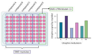
Created with BioRender.com
In summary, while there is support and enthusiasm for the techniques and methodological approach of the study, the future use of this single line might be dubious and could be strengthened if additional lines are generated.
We share the reviewer’s enthusiasm for this approach, and we have included in the new version of the manuscript further characterization of this new cell culture that we think would demonstrate its usefulness better.
Author Response refers to a revised version of the manuscript, Version 3, which was posted October 23, 2020.
Summary:
Serra-Marques, Martin et al. investigate the individual and cooperative roles of specific kinesins in transporting Rab6 secretory vesicles in HeLa cells using CRISPR and live-cell imaging. They find that both KIF5B and KIF13B cooperate in transporting Rab6 vesicles, but Eg5 and other kinesin-3s (KIF1B and KIF1C) are dispensable for Rab6 vesicle transport. They show that both KIF5B and KIF13B localize to these vesicles and coordinate their activities such that KIF5B is the main driver of the cargos on older, MAP7-decorated microtubules, and KIF13B takes over as the main transporter on freshly-polymerized microtubule ends that are largely devoid of MAP7. Interestingly, their data also indicate that KIF5B is important for controlling Rab6 vesicle size, which KIF13B cannot rescue. By analyzing subpixel localization of the motors, they find that the motors localize to the front of the vesicle when driving transport, but upon directional cargo switching, KIF5B localizes to the back of the vesicle when opposing dynein. Overall, this paper provides substantial insight into motor cooperation of cargo transport and clarifies the contribution of these distinct classes of motors during Rab6 vesicle transport.
We thank the reviewers for their thoughtful and constructive suggestions, and for the positive feedback.
Reviewer #1:
In their manuscript, Serra-Marques, Martin, et al. investigate the individual and cooperative roles of specific kinesins in transporting Rab6 vesicles in HeLa cells using CRISPR and live-cell imaging. They find that both KIF5B and KIF13B cooperate in transporting Rab6 vesicles, but KIF5B is the main driver of transport. In these cells, Eg5 and other kinesin-3s (KIF1B and KIF1C) are dispensable for Rab6 vesicle transport. They find that both KIF5B and KIF13B are present on these vesicles and coordinate their activities such that KIF5B is the main driver of the cargos on older, MAP7-decorated MTs, and KIF13B takes over as the main transporter on freshly-polymerized MT ends that are largely devoid of MAP7. Interestingly, their data also indicate that KIF5B is important for controlling Rab6 vesicle size, which KIF13B cannot rescue. Upon cargo switching from anterograde to retrograde transport, KIF5B, but not KIF13B, engages in mechanical competition with dynein. Overall, this paper provides substantial insight into motor cooperation of cargo transport and clarifies the contribution of these distinct classes of motors during Rab6 vesicle transport. The experiments are well-performed and the data are of very high quality.
Major Comments:
1) In Figure 5, it is very interesting that only KIF5B opposes dynein. It would be informative to determine which kinesin was engaged on the Rab6 vesicle before the switch to the retrograde direction. Can the authors analyze the velocity of the run right before the switch to the retrograde direction? If the velocity corresponds with KIF5B (the one example provided seems to show a slow run prior to the switch), this could indicate that KIF5B opposes dynein more actively because KIF5B was the motor that was engaged at the time of the switch. Or if the velocity corresponds with KIF13B, this could indicate that KIF5B becomes specifically engaged upon a direction reversal. In any case, an analysis of the speed distributions before the switch would provide insight into vesicle movement and motor engagement before the change in direction.
Directional switching was only analyzed in rescue experiments, where the vesicles were driven by either KIF5B alone or by KIF13B alone, and the speeds of vesicles were representative of these motors (please see panels on the right). The number of vesicle runs where two motors were detected simultaneously (KIF5B vs KIF13B in Figure 5G,H,J) were significantly lower, and therefore, unfortunately we could not perform the analysis of their directional switching with sufficient statistical power.
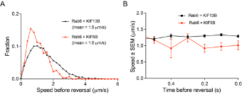
2) One of the most interesting aspects of this paper is the different lattice preferences for KIF5B, which shows runs predominantly on "older" polymerized MTs decorated by MAP7, and for KIF13B, whose runs are predominantly restricted to newly polymerized MTs that lack MAP7. The results in Figure 8 suggest a potential switch from KIF5B to KIF13B motor engagement upon a change in lattice/MAP7 distribution. In general, do the authors observe the fastest runs at the cell periphery, where there should be a larger population of freshly polymerized MTs? For Figure 4E, are example 1 and example 2 in different regions of the cell?
This is indeed a very interesting point and we have considered it carefully. As can be seen in Figure 8B (grey curve), vesicle speed remains relatively constant along the cell radius in control HeLa cells. We note, however, that our previous work has shown that in these cells microtubules are quite stable even at the cell periphery, due to the high activity of the CLASP-containing cortical microtubule stabilization complex (Mimori-Kiyosue et al., 2005, Journal of Cell Biology, PMID: 15631994; van der Vaart et al., 2013, Developmental Cell, PMID: 24120883). We therefore hypothesized that changes in vesicle speed distribution along the cell radius would be more obvious in cells with highly dynamic microtubule networks and performed a preliminary experiment in MRC5 human lung fibroblasts, which have a very sparse and dynamic microtubule cytoskeleton (Splinter et al., 2012, Molecular Biology of the Cell, PMID: 22956769). As shown in the figure below, we indeed found that vesicles move faster at the cell periphery. Even though these data are suggestive, characterization of this additional cell model goes beyond the scope of the current study, and we prefer not to include them in the manuscript.
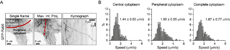
In Figure 4E, the two examples are from different cells, and were both recorded at the cell periphery. The difference in vesicle speeds reflects general speed variability.
Do the authors think the intermediate speeds are a result of the motors switching roles? Additional discussion would help the reader interpret the results.
Presence of intermediate speeds of cargos driven by multiple motors of two types is most clear in Figure 3F-H, where multiple and different ratios of KIF5B and KIF13B motors are recruited to peroxisomes. As can be seen in Fig. 3G, the kymographs in these conditions are “smooth” and no evidence of motor switching can be detected at this spatiotemporal resolution. On the other hand, it has been previously beautifully shown by the Verhey lab that when artificial cargos are driven by just two motor molecules of different nature, switching does occur (Norris et al., 2014, Journal of Cell Biology, PMID: 25365993). This point is emphasized on page 12 of the revised manuscript. These data suggest that motors working in teams show different properties, and more detailed biophysical analysis will be needed to understand them.
Reviewer #2:
The manuscript by Serra-Marques, Martin, et al provides a tour de force in the analysis of vesicle transport by different kinesin motor proteins. The authors generate cell lines lacking a specific kinesin or combination of kinesins. They analyze the distribution and transport of Rab6 as a marker of most, if not all, secretory vesicles and show that both KIF5B and KIF13B localize to these vesicles and describe the contribution of each motor to vesicle transport. They show that the motors localize to the front of the vesicle when driving transport whereas KIF5B localizes to the back of the vesicle when opposing dynein. They find that KIF5B is the major motor and its action on "old" microtubules is facilitated by MAP7 whereas KIF13B facilitates transport on "new" microtubules to bring vesicles to the cell periphery. The manuscript is well-written, the data are properly controlled and analyzed, and the results are nicely presented. There are a few things the authors could do to tie up loose ends but these would not change the conclusions or impact of the work and I only have a couple of clarifying questions.
In Figure 2E, it seems like about half of the KIF5B events start at or near the Golgi whereas most of the KIF13B events are away from the Golgi? Did the authors find this to be generally true or just apparent in these example images?
We sincerely apologize for the misunderstanding here. To automatically track the vesicles, we had to manually exclude the Golgi area. Moreover, only processive and not complete tracks are shown. Therefore, no conclusions can be made from these data on the vesicle exit from the Golgi. We have indicated this clearly in the Results (page 8) and Discussion (page 21) of the revised manuscript and included more representative images in the revised Figure 2E.
In Figure 8G, the tracks for KIF13B-380 motility are difficult to see, which is surprising as KIF13B has been shown to be a superprocessive motor. Is this construct a dimer? If not, do the authors interpret the data as a high binding affinity of the monomer for new microtubules and if so, do they have any speculation on what could be the molecular mechanism? It appears as if KIF13B-380 and EB3 colocalize at the plus ends for a period of time before both are lost but then quickly replenished. Is this common?
KIF13B-380 construct used here contains a leucine zipper from GCN4 and is therefore dimeric. In the revised version of the paper, we have indicated this more clearly in the Results section on page 17 of the revised manuscript. KIF13B-380 does show processive motility, although this is difficult to see close to the outermost microtubule tip as the motor tends to accumulate there. This does not necessarily correlate with a strong accumulation of EB3, likely because EB3 signal is more sensitive to the dynamic state of the microtubule (it diminishes when microtubule growth rate decreases). We now provide a kymograph in Fig. 8G where the processive motility of KIF13B-380 is clearer.
Reviewer #3:
Serra-Marques and co-authors use CRISPR/Cas9 gene editing and live-cell imaging to dissect the roles of kinesin-1 (KIF5) and kinesin-3 (KIF13) in the transport of Rab6-positive vesicles. They find that both kinesins contribute to the movement of Rab6 vesicles. In the context of recent studies on the effect of MAP7 and doublecortin on kinesin motility, the authors show that MAP7 is enriched on central microtubules corresponding to the preferred localization of constitutively-active KIF5B-560-GFP. In contrast, KIF13 is enriched on dynamic, peripheral microtubules marked by EB3.
The manuscript provides needed insight into how multiple types of kinesin motors coordinate their function to transport vesicles. However, I outline several concerns about the analysis of vesicle and kinesin motility and its interpretation below.
Major concerns:
1) The metrics used to quantify motility are sensitive to tracking errors and uncertainty. The authors quantify the number of runs (Fig. 2D,F; 7C) and the average speed (Fig. 3A,B,D,E,H). The number of runs is sensitive to linking errors in tracking. A single, long trajectory is often misrepresented as multiple shorter trajectories. These linking errors are sensitive to small differences in the signal-to-noise ratio between experiments and conditions, and the set of tracking parameters used. The average speed is reported only for the long, processive runs (tracks>20 frames, segments<6 frames with velocity vector correlation >0.6). For many vesicular cargoes, these long runs represent <10% of the total motility. In the 4X-KO cells, it is expected there is very little processive motility, yet the average speed is higher than in control cells. Frame-to-frame velocities are often over-estimated due to the tracking uncertainty. Metrics like mean-squared displacement are less sensitive to tracking errors, and the velocity of the processive segments can be determined from the mean-squared displacement (see for example Chugh et al., 2018, Biophys. J.). The authors should also report either the average velocity of the entire run (including pauses), or the fraction of time represented by the processive segments to aid in interpreting the velocity data.
Two stages of the described tracking and data processing are responsible for the extraction of processive runs: the “linking” method used during the tracking, and the “trajectory segmentation” method, applied to the obtained tracks. The detection and linking of vesicles have been performed using our previously published tracking method (Chenouard et al., 2014, Nature Methods, PMID: 24441936). Our linking method uses multi-frame data association, taking into account detections from four subsequent image frames in order to extend and create a trajectory at any given time. This allows for dealing with temporal disappearance of particles (missing detections) for 1-2 frames and avoiding creation of breaks in longer trajectories. The method is robust to noise, spurious and missing detections and had been fully evaluated in the aforementioned paper (Chenouard et al., 2014) showing excellent performance compared to other tracking methods.
Having the trajectories describing the behavior of each particle, the track segmentation method had been applied to split each trajectory into a sequence of smaller parts (tracklets) describing processive runs and pieces of undirected (diffusive) motion. The algorithm that we used was validated earlier on an artificial dataset (please see Fig.S2e in Katrukha et al., Nat Commun 2017, PMID: 28322225). The chosen parameters were in the range where the algorithm provided less than 10% of false positives. Since the quantified and reported changes in the number of runs are six-fold (Fig.2D,F), we are quite certain that this estimated error (inherent to all automatic image analysis methods) does not affect our conclusions. Moreover, it is consistent with visual observations and manual analysis of representative movies.
Further, we agree that frame-to-frame velocities are often somewhat over-estimated due to the tracking uncertainty. We are aware of such overestimation which is very difficult to avoid. In our case, we estimated (using a Monte Carlo simulation) that such overestimation will positively bias the average not more than 3-6%. Since we focus not on the absolute values of velocities, but rather on the comparison between different conditions, such biasing will be present in all estimates of average velocity and will not affect the presented conclusions.
The usage of mean square displacement (MSD) to analyze trajectories containing both periods of processive runs and diffusive motion is confusing, since it represents average value over whole trajectories, resulting in the MSD slope which is in the range of 1.5 (i.e. between 1, diffusive and 2, processive; please see Fig.2c in Katrukha et al., 2017, Nature Communications, PMID: 28322225). Therefore, initial segmentation of trajectories is necessary, as it was performed in the paper by Chugh et al (Chugh et al., 2018, Biophysical Journal, PMID: 30021112; please see Fig.2e in that paper), suggested by the reviewer. In this paper the authors used an SCI algorithm, which is very similar to our analysis, relying on temporal correlations of velocities. Indeed, MSD analysis of only processive segments is less sensitive to tracking errors, but it reports an average velocity of the whole population of runs. This method is well suited if one would expect monodisperse velocity distribution (the case in Chugh et al, where single motor trajectories are analyzed). If there are subpopulations with different speeds (as we observed for Rab6 by manual kymograph analysis), this information will be averaged out. Therefore, we used histogram/distribution representations for our speed data, which in our opinion represents these data better.
Finally, we fully agree with the reviewers that the fractions of processive/diffusive motion should be reported. In the revised version, we have added new plots to the revised manuscript (Figure 2G-I, Figure 2 - figure supplement 2G) illustrating these data for different conditions. Our data fully support the reviewer’s statement that processive runs represent less than 10% of total vesicle motility (new Figure 2G). As could be expected, the total time vesicles spent in processive motion and the percentage of trajectories containing processive runs strongly depended on the presence of the motors (new Figure 2H,I). However, within trajectories that did have processive segments, the percentage of processive movement was similar (new Figure 2I).
We note that while our analysis is geared towards identification and characterization of processive runs (which was verified manually), analysis of diffusive movements poses additional challenges and is even more sensitive to linking errors. Therefore, we do not make any strong quantitative conclusions about the exact percentage and the properties of diffusive vesicle movements, and their detailed studies will require additional analytic efforts.
2) The authors show that transient expression of either KIF13B or KIF5B partially rescues Rab6 motility in 4X-KO cells and that knock-out of KIF13B and KIF5B have an additive effect. They also analyze two vesicles where KIF13B and KIF5B co-localize on the same vesicle. The authors conclude that KIF13B and KIF5B cooperate to transport Rab6 vesicles. However, the nature of this cooperation is unclear. Are the motors recruited sequentially to the vesicles, or at the same time? Is there a subset of vesicles enriched for KIF13B and a subset enriched for KIF5B? Is motor recruitment dependent on localization in the cell? These open questions should be addressed in the discussion.
Unfortunately, only fluorescent motors and not the endogenous ones can be detected on vesicles, so we cannot make any strong statements on this issue. Since KIF13B can compensate for the absence of KIF5B, it can be recruited to the vesicle when it emerges from the Golgi apparatus. However, in normal cells, KIF5B likely plays a more prominent role in pulling the vesicles from the Golgi, as Rab6 vesicles generated in the presence of KIF5B are larger (Figure 5I). We show in Figure 1G,H that KIF13B does not exchange on the vesicle and stays on the vesicle until it fuses with the plasma membrane. These data suggest that once recruited, KIF13B stays bound to the vesicle. Obtaining such data for KIF5B is more problematic because fewer copies of this motor are typically recruited to the vesicle (Figure 4B) and its signal is therefore weaker. Further research with endogenously tagged motors and highly sensitive imaging approaches will be needed to address the important open questions raised by the reviewer. We have added these points to the Discussion on pages 19 and 21 of the revised manuscript.
3) The authors suggest that KIF5B transports Rab6 vesicles along centrally-located microtubules while KIF13B drives transport on peripheral microtubules. Is the velocity of Rab6 vesicles different on central and peripheral microtubules in control cells?
As indicated in our answer to Major Comment 2 of Reviewer 1, we show in Figure 8B (grey curve) that vesicle speed remains relatively constant along the cell radius in control HeLa cells. We note, however, that our previous work has shown that in these cells microtubules are quite stable even at the cell periphery, due to the high activity of the CLASP-containing cortical microtubule stabilization complex (Mimori-Kiyosue et al., 2005, Journal of Cell Biology, PMID: 15631994; van der Vaart et al., 2013, Developmental Cell, PMID: 24120883). We therefore hypothesized that changes in vesicle speed distribution along the cell radius would be more obvious in cells with highly dynamic microtubule networks and performed a preliminary experiment in MRC5 human lung fibroblasts, which have a very sparse and dynamic microtubule cytoskeleton (Splinter et al., 2012, Molecular Biology of the Cell, PMID: 22956769). As shown in the figure above, we indeed found that vesicles move faster at the cell periphery.
4) The imaging and tracking of fluorescently-labeled kinesins in cells as shown in Fig. 4 is impressive. This is often challenging as kinesin-3 forms bright accumulations at the cell periphery and there is a large soluble pool of motors, making it difficult to image individual vesicles. The authors should provide additional details on how they addressed these challenges. Control experiments to assess crosstalk between fluorescence images would increase confidence in the colocalization results.
Imaging of vesicle motility was performed using TIRF microscopy focusing on regions where no strong motor accumulation was observed. We have little cross-talk between red and green channels, but channel cross talk in the three-color images shown in Figure 4E was indeed a potential concern. To address this potential issue, we performed the appropriate controls and added a new figure to the revised manuscript (Figure 4 – figure supplement 1). We conclude that we can reliably simultaneously detect blue, green and red channels without significant cross-talk on our microscope setup.
Summary
This manuscript examines how N-linked glycosylation regulates the binding of polysaccharide hyaluronan (HA) to cell surface receptor CD44, to conclude that multiple sites exist but are controlled by the nature of the glycosylation. The reviewers appreciated many aspects of the work, but they have raised serious concerns about the experimental and simulation design. The reviewers suggested that the proposed alternative binding site may not be biologically relevant, as the relevant CD44-HA interactions are multivalent and cannot be supported by that site. They also suggested that the findings are not well supported by the NMR experiments, which could have been extended to allow comparisons of the glycosylation patterns hypothesised. Moreover, the MD simulations, despite being considerable in size, were limited in sampling different possibilities without bias from the initial HA placement, and there is not enough data to convince the readers of thorough sampling and reproducibility.
We understand the concerns raised in the review process. However, these concerns can be readily explained and fixed, as we explain below and are briefly introduced here.
• Our data are compatible with the currently accepted multivalent interaction of hyaluronan with several CD44 receptors. The argument that our data goes against it stems from an unfortunate figure provided in the first version of the manuscript. This figure suggested that a bound hyaluronan would not be able to span the length the protein in the upright binding mode. That is not true. We now show another, and more relevant snapshot where the bound hyaluronan indeed spans the length of HABD. Hence, we show that multivalent interaction is not precluded by the upright binding mode.
• We also clarify how our extensive simulation data were designed to avoid any bias. We admit that this was not obvious in the phrasing of our previous version.
• Many of the raised issues stem from the lack of certain critical simulations. We have now added these simulations into the revision.
Below we summarize the main issues raised by the reviewers, accompanied by our responses on how we have fixed them in the revised version of the manuscript.
Reviewer #1
The authors use MD simulations and NMR to study the cell surface adhesion receptor CD44 with the purpose of understanding the binding of carbohydrate polymer, hyaluronan (HA). In particular, this study focuses on the effects of N-glycosylation of the CD44 glycoprotein on potential HA binding. The authors previously proposed two lower affinity HA binding modes as alternatives to the primary mode seen in the crystal structure of the HA binding domain of CD44, driven by different arginine interactions, but overlapping with glycosylation sites that will affect HA binding. This study suggests that, because the canonical site appears blocked by glycans attached to the surface, HA would instead likely bind to an alternate parallel site with lower affinity, thus changing receptor affinity. The authors do not study HA binding to the glycosylated form directly, but undertake simulations of bound glycans to draw their conclusion. They do, however, place HA near the non-glycosylated CD44 in simulations, although it is not clear that MD sampling has been designed to provide unbiased observations of HA binding, or how the simulations help explain the NMR experiments.
To better highlight the message, we left out a significant portion of our total simulation data from the initial version of the manuscript. We have now added e.g. simulations of HA binding to the glycosylated form into our revised manuscript. Furthermore, we are confident that our design of the simulation systems allows unbiased sampling of the binding surface. That is, the hyaluronan hexamers were initially placed several nanometres away from the protein surface. After this, they were allowed to spontaneously sample the space and find their respective binding sites during the course of the simulations. They were not placed into the binding sites manually. However, there was a one system with two HA hexamers from which the other was placed into the canonical binding groove. This was done to test where the freely floating hexamer would bind when the primary binding site is taken. These points are illustrated more clearly in the new version of the manuscript. Finally, all our simulation data is publicly available (see the DOIs provided in the paper).
The data rely on libraries of MD simulation, which are substantial, with several replicas of a microsecond each. But what have these simulations really proved with reliability? Figure 2a shows that, while glycans stay roughly where they started, they are dynamic and cover much of the canonical HA binding site, which may be the case. From this the authors imply that the crystallographic site is significantly obstructed, the lower-affinity upright mode remains most accessible, and that the level of occlusion of the main site depends on the degree of glycosylation and size of the oligosaccharides. However, a full simulation of HA binding to this glycosylated surface was not attempted. It would have been good to see the glycans actually block unbiased simulation of canonical binding to the crystallographic site on long timescales (not being dislodged), but allow alternative binding to the parallel site, without initial placement there.
Commenting both points 1.1 and 1.2, we cropped a large portion of our simulation data from the initial version of the manuscript in order to better highlight the current message. However, we do have extensive simulation data of hyaluronan binding spontaneously to CD44 with different glycosylation patterns. For example, see Figure A below where HA is bound to glycosylated CD44-HABD. These data have been carefully analysed and incorporated into the revised manuscript.
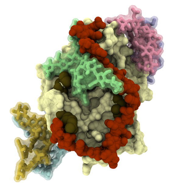
Figure A. A representative binding pose between HA oligomer (dark red) and glycosylated (light blue, yellow, green, pink and purple) CD44-HABD (pale surface) extracted from our simulations.
HA was, however, added to the non-glycosylated CD44-HABD surface in simulations, but no clear data is shown to illustrate the extent of sampling, convergence and reproducibility, beyond some statistical analysis of contacts. It seems a total of 30 microseconds of the non-glycosylated protein with 2 or 3 nearby HA placed was run, leading to contacts. But how well did these 30 simulations sample HA movement and relative binding to sites, if at all? Figure 4 suggests that the HA stay where they have been put. As the MD is the dominant source of data for the paper, the extent of sampling and how the outcomes depend on the initial placement of molecules requires proof. Was any sampling of HA movement, such as between canonical and alternative parallel conformations seen in MD?
It is important to note that, in the non-glycosylated systems, the hyaluronan hexamers were initially placed several nanometres away from the protein surface. After this, they were allowed to spontaneously sample the space and find their respective binding sites during the course of the simulations. That is, they were not manually placed into the binding sites. We have changed the manuscript to better illustrate this key point.
We have also made the simulation data publicly available (see the DOIs provided in the paper). After inspection of the simulations, we are confident that the reviewers will agree that the results are reliable and do not suffer from convergence problems that could compromise the message we provide.
Moreover, we have even more simulation replicas ready with slightly different initial conditions that provide the same qualitative picture, see Figure B below (compare with Figure 4c in the original submission where one of the hyaluronan hexamers was initially placed in the crystallographic binding site). In these simulations, the hexamers have enhanced contacts with the crystallographic and upright mode residues despite being initially placed far from these binding sites. These simulations were already part of the manuscript.
Figure B. Hyaluronate-perturbed residues in the simulations. The colored surface displays the probability of a given residue to be in contact with HA6 in our additional simulations, where three hyaluronan hexamers were placed in solution far from the binding site.
The NMR is suggested to show that a short HA hexamer can bind to non-glycosylated CD44-HABD simultaneously in several modes at distinct binding sites, and that MD "correlates" with this. But is this MD biased by initial choices of where and how many HAs are placed, given HA movement is likely not well sampled?
The hyaluronan hexamers were initially placed several nanometers away from the binding sites. They were not placed into these binding sites manually. During the simulations the hexamers displayed several binding and unbinding events as they were spontaneously sampling the space and finding their respective binding sites during the course of the simulations.
While we saw multiple binding events to the proposed binding sites, the short size of the hyaluronan fragments was likely not enough for stable binding as the fragments often dissociated within few hundreds of nanoseconds. These points are now more clearly presented in the revised manuscript.
No MD seems to have been used to examine the blocking or lack thereof by antibody MEM-85 in glycosylated or non-glycosylated CD44.
This is not feasible using MD simulations, since the structure of the antibody is not available. Fortunately, there is no need for it, as we have direct and reliable experimental evidence using NMR as provided in the manuscript and in our previous work (Skerlova et.al. 2015; doi: 10.1016/j.jsb.2015.06.005). We therefore know where the antibody binds in CD44.
Reviewer #2
This manuscript is focused on understanding how N-linked glycosylation regulates the binding of the (very large) polysaccharide hyaluronan (HA) to its major cell surface receptor CD44, a question relevant, for example to the role of CD44 in mediating leukocyte migration in inflammation. The paper concludes that multiple binding sites for HA exist and that their occupancy is determined by the nature of the glycosylation, a suggestion first made by Teriete et al. (2004). The work is based on atomistic simulations with different glycan compositions and NMR spectroscopy on a non-glycosylated CD44 HA-binding domain (HABD) expressed in E. coli. While the question being researched is interesting and of biological relevance, there are flaws in the work.
The relevance also stems from the increasing applicability of HA in many biomedical devices and treatment strategies, such as tissue scaffolds and HA-coated nanoparticles for targeted drug delivery. However, we respectfully disagree with the proposed flaws. We address these suggested issues point-by-point in sections 2.2–2.5.
The paper describes how the well-established HA-binding site on CD44 (determined by a co-crystal structure; Banerji et al., 2007) is blocked by N-linked glycosylation (principally at N25 with a contribution from glycans at N100 and N110) and how certain glycans favour binding at a completely distinct binding site that lies perpendicular to the canonical 'crystallographic' binding site. This alternative 'upright' binding site, which has been proposed previously by the authors (Vuorio et al., 2017), needs further supporting experimental data.
Indeed, a characterization of the upright mode can be found from (Vuorio et al., 2017. PloS CB. 13:7). This characterization is based on mircoseconds of unbiased MD simulation data as well as extensive free energy calculations. We for example analysed the most important interactions, orientations of the sugar rings, and binding affinities. These data indicate that while the upright binding mode is weaker than the canonical binding mode (Banerji et al., 2007), it has good shape complementarity between the protein, with e.g. most of the sugar rings lying flat on the surface of the protein, indicating that it might have biological relevance.
The supporting experimental data is presented in the current publication. It has been improved and clarified for the revised version of the manuscript.
Firstly, unlike the 'crystallographic' binding site that forms an open-ended shallow groove on the surface of the protein allowing polymeric HA to bind (and multivalent interactions to take place), the 'upright' binding site is closed at one end and can thus only accommodate the reducing end of the polysaccharide (as apparent from Appendix 1 Figure 1). Its configuration means that it would be impossible for this mode of binding to allow multivalent interactions with polymeric HA. This is a major problem since biologically relevant CD44-HA interactions are multivalent where a single HA polymer interacts with a large number of CD44 molecules (e.g. see Wolny et al., 2010 J. Biol. Chem. 285, 30170-30180). So even if this binding site existed, an interaction between a single CD44 molecule on the cell surface with the reducing terminus of an HA polymer would be exceptionally weak.
We have data to show that our proposed secondary binding mode does not preclude multivalent CD44-hyaluronan interactions. This multivalent interaction, where a long hyaluronan binds simultaneously to several CD44 moieties, is important, and our secondary mode is compatible with it, see the new Figure C below. We acknowledge that our Figure 1 in the Appendix 1 was not sufficiently clear on this matter. That figure illustrated a structure of one possible CD44-hyaluronan complex obtained from just one of our simulations. However, we have a number of related CD44-hyaluronan complexes from other simulations where the bound ligand spans the full length of the protein, showing that the binding site can accommodate more than just the reducing end of the polysaccharide, and this is highlighted in the attached Figure C. Therefore, multivalent binding is not precluded by the upright binding mode. Unfortunately, the figure depicted in the SI of the original manuscript was misleading. To avoid this issue, it has been replaced in the revised manuscript.
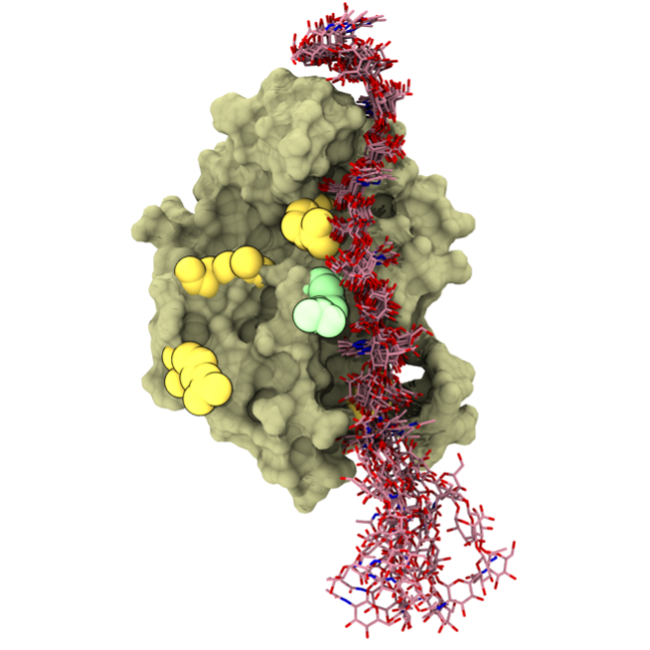
Figure C. The secondary CD44-hyaluronan binding mode.
Secondly the NMR experiments performed in this study, purporting to provide evidence for multiple modes of binding, are problematic. Why weren't differentially glycosylated proteins used, i.e. where individual sites were mutated (e.g. +/- N25); this would have allowed comparisons of the glycosylation patterns hypothesised (based on the computer simulations) to favour the 'crystallographic' versus 'upright' modes.
Indeed, NMR experiments with glycosylated material would be ideal, but obtaining the required quantities of isotopically labelled protein with a homogeneous glycosylation pattern is not possible even using the state-of-the-art technology. In addition, the substantially increased molecular weight of the glycosylated protein would be out of the experimental window accessible by NMR spectroscopy. We strongly believe that the message of the paper is already sustained by a combination of our observations based on NMR experiments and MD simulation techniques together with the available literature data as detailed in Appendix A (see below).
While being aware of the difficulties of dealing with glycosylated CD44 using NMR, we designed a way to bypass this issue by combining multiple data from different experimental and simulation setups. All the data support the claims and conclusions made in our paper, see appendix A of this rebuttal. The existence of a weaker binding mode promoted upon glycosylation due to the primary binding site being covered is compatible with all available experimental and simulation data.
Furthermore, previous NMR studies have shown that the binding of HA to CD44 causes a considerable number of chemical shift changes due to the induction of a large conformational change in the protein (Teriete et al., 2004; Banerji et al., 2007), making it very difficult to identify amino acids directly involved in HA binding based on the NMR data. Moreover, this conformational change has been fully characterised for mouse CD44 with structures available in the absence and presence of HA (Banerji et al., 2007); this information should have been used to inform the interpretation of the shift mapping. In fact, the way in which the shift mapping data are interpreted is simplistic and doesn't fully take account of the reasons that NMR spectra can exhibit different exchange regimes.
We interpreted the NMR data very carefully. We are aware of the extent of conformational changes induced by HA binding in CD44-HABD, in fact, we identified them as a molecular mechanism underlying the mode of action for the MEM-85 antibody (Skerlova et.al. 2015; doi: 10.1016/j.jsb.2015.06.005). Therefore, we focused on the differential changes in the NMR signal positions of surface exposed residues upon titration with HA and MEM-85. We also observed different exchange regimes that allowed us to discriminate between different HA binding sites. We emphasized these points in the revised manuscript.
Reviewer #3
Vuorio and colleagues combine atomic resolution molecular dynamics simulations and NMR experiments to probe how glycosylation can bias binding of hyaluronan to one of several binding sites/modes on the CD44 hyaluronan binding domain. The results are of interest specifically to the field of CD44 biophysics and more generally to the broad field of glycosylation-dependent protein-ligand binding. The manuscript is clearly written, and the combination of data from computational and experimental methodologies is convincing. I especially commend the authors on the thorough molecular dynamics work, wherein they ran multiple simulations at microsecond timescale and tried different force fields to minimize the likelihood of their findings being an artifact of a particular force field.
The use of multiple force fields was indeed meant to alleviate potential force field specific issues. Likewise, the use of multiple simulation repeats with different starting positions and randomized atom velocities were meant to provide comprehensive statistics, minimizing the chances of over-interpreting any isolated phenomena.
Appendix A: Summary of the logic of the research procedure together with the experimental, simulation and literature results supporting each step.
1) Non-glycosylated CD44 binds HA *(NMR experiments) *
2) Non-glycosylated CD44 also binds HA in the presence of MEM-85 (NMR experiments)
3) Glycosylated CD44s that bind HA do not bind HA in the presence of MEM-85 (from literature [J. Bajorath, B. Greenfield, S. B. Munro, A. J. Day, A. Aruffo, Journal of Biological Chemistry 273, 338 (1998).]).
4) We show the MEM-85 binding site in non-glycosylated CD44 to be far from the canonical crystallographic binding region (NMR experiments). This MEM-85 binding site region is mostly inaccessible to typical N-glycans found in CD44 (MD simulation). Therefore, we expect that MEM-85 binds glycosylated CD44 in the same region. *(Our working hypothesis) *
5) Taken together, the above points indicate that MEM-85 covers at least partially the relevant HA binding mode in glycosylated CD44, which has zero overlap with the crystallographic mode. This supports the idea of an alternative binding mode to the crystallographic mode which must be readily available for glycosylated CD44. (Our finding)
6) Furthermore, heavily glycosylated CD44 variants cover a significant fraction of the crystallographic mode binding region (MD simulation), potentially making it unavailable for HA binding. This explains why non-glycosylated CD44 binds HA in the presence of MEM-85 (i.e., crystallographic mode is free), while glycosylated CD44 does not (i.e., crystallographic mode is covered with N-glycans). The upright region, on the other hand, experiences only minor coverage by the N-glycans in the glycosylated CD44 and is thus free to bind the ligand (MD simulations).
7) Non-glycosylated CD44 binds HA simultaneously with the crystallographic mode and the upright mode when exposed to high concentrations of small hyaluronan hexamers *(NMR titration and MD simulations). *
8) Pinpointing the position of the residues that experience the largest chemical shift during the titration experiments using non-glycosylated CD44 clearly shows the fingerprint of the canonical crystallographic mode but also a region compatible with our proposed upright mode (NMR titration experiments). These results are compatible with our simulations of several hyaluronan hexamers (MD simulation).
9) Upright binding mode is accessible to hyaluronan binding in the glycosylated CD44 (MD simulations shown in this letter that could be included to the paper if deemed necessary).
Glycosylation, and glycoscience in general, is one of the most challenging topics to understand in life sciences. We believe that our paper makes a very significant contribution to this area of research in the context of a central research problem and is exceptionally able to provide an atomic-level description of the HA-CD44 interaction under unambiguously known conditions.
Author Response:
Evaluation Summary:
Since DBS of the habenula is a new treatment, these are the first data of its kind and potentially of high interest to the field. Although the study mostly confirms findings from animal studies rather than bringing up completely new aspects of emotion processing, it certainly closes a knowledge gap. This paper is of interest to neuroscientists studying emotions and clinicians treating psychiatric disorders. Specifically the paper shows that the habenula is involved in processing of negative emotions and that it is synchronized to the prefrontal cortex in the theta band. These are important insights into the electrophysiology of emotion processing in the human brain.
The authors are very grateful for the reviewers’ positive comments on our study. We also thank all the reviewers for the comments which has helped to improve the manuscript.
Reviewer #1 (Public Review):
The study by Huang et al. report on direct recordings (using DBS electrodes) from the human habenula in conjunction with MEG recordings in 9 patients. Participants were shown emotional pictures. The key finding was a transient increase in theta/alpha activity with negative compared to positive stimuli. Furthermore, there was a later increase in oscillatory coupling in the same band. These are important data, as there are few reports of direct recordings from the habenula together with the MEG in humans performing cognitive tasks. The findings do provide novel insight into the network dynamics associated with the processing of emotional stimuli and particular the role of the habenula.
Recommendations:
How can we be sure that the recordings from the habenula are not contaminated by volume conduction; i.e. signals from neighbouring regions? I do understand that bipolar signals were considered for the DBS electrode leads. However, high-frequency power (gamma band and up) is often associated with spiking/MUA and considered less prone to volume conduction. I propose to also investigate that high-frequency gamma band activity recorded from the bipolar DBS electrodes and relate to the emotional faces. This will provide more certainty that the measured activity indeed stems from the habenula.
We thank the reviewer for the comment. As the reviewer pointed out, bipolar macroelectrode can detect locally generated potentials, as demonstrated in the case of recordings from subthalamic nucleus and especially when the macroelectrodes are inside the subthalamic nucleus (Marmor et al., 2017). However, considering the size of the habenula and the size of the DBS electrode contacts, we have to acknowledge that we cannot completely exclude the possibility that the recordings are contaminated by volume conduction of activities from neighbouring areas, as shown in Bertone-Cueto et al. 2019. We have now added extra information about the size of the habenula and acknowledged the potential contamination of activities from neighbouring areas through volume conduction in the ‘Limitation’:
"Another caveat we would like to acknowledge that the human habenula is a small region. Existing data from structural MRI scans reported combined habenula (the sum of the left and right hemispheres) volumes of ~ 30–36 mm3 (Savitz et al., 2011a; Savitz et al., 2011b) which means each habenula has the size of 2~3 mm in each dimension, which may be even smaller than the standard functional MRI voxel size (Lawson et al., 2013). The size of the habenula is also small relative to the standard DBS electrodes (as shown in Fig. 2A). The electrodes used in this study (Medtronic 3389) have electrode diameter of 1.27 mm with each contact length of 1.5 mm, and contact spacing of 0.5 mm. We have tried different ways to confirm the location of the electrode and to select the contacts that is within or closest to the habenula: 1.) the MRI was co-registered with a CT image (General Electric, Waukesha, WI, USA) with the Leksell stereotactic frame to obtain the coordinate values of the tip of the electrode; 2.) Post-operative CT was co-registered to pre-operative T1 MRI using a two-stage linear registration using Lead-DBS software. We used bipolar signals constructed from neighbouring macroelectrode recordings, which have been shown to detect locally generated potentials from subthalamic nucleus and especially when the macroelectrodes are inside the subthalamic nucleus (Marmor et al., 2017). Considering that not all contacts for bipolar LFP construction are in the habenula in this study, as shown in Fig. 2, we cannot exclude the possibility that the activities we measured are contaminated by activities from neighbouring areas through volume conduction. In particular, the human habenula is surrounded by thalamus and adjacent to the posterior end of the medial dorsal thalamus, so we may have captured activities from the medial dorsal thalamus. However, we also showed that those bipolar LFPs from contacts in the habenula tend to have a peak in the theta/alpha band in the power spectra density (PSD); whereas recordings from contacts outside the habenula tend to have extra peak in beta frequency band in the PSD. This supports the habenula origin of the emotional valence related changes in the theta/alpha activities reported here."
We have also looked at gamma band oscillations or high frequency activities in the recordings. However, we didn’t observe any peak in high frequency band in the average power spectral density, or any consistent difference in the high frequency activities induced by the emotional stimuli (Fig. S1). We suspect that high frequency activities related to MUA/spiking are very local and have very small amplitude, so they are not picked up by the bipolar LFPs measured from contacts with both the contact area for each contact and the between-contact space quite large comparative to the size of the habenula.
A
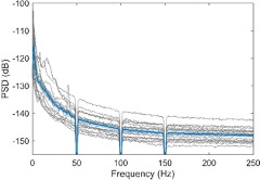
B
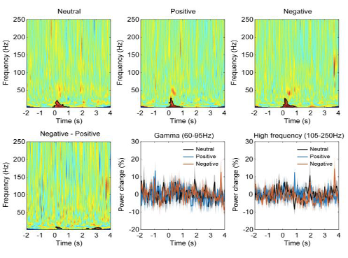
Figure S1. (A) Power spectral density of habenula LFPs across all time period when emotional stimuli were presented. The bold blue line and shadowed region indicates the mean ± SEM across all recorded hemispheres and the thin grey lines show measurements from individual hemispheres. (B) Time-frequency representations of the power response relative to pre-stimulus baseline for different conditions showing habenula gamma and high frequency activity are not modulated by emotional
References:
Savitz JB, Bonne O, Nugent AC, Vythilingam M, Bogers W, Charney DS, et al. Habenula volume in post-traumatic stress disorder measured with high-resolution MRI. Biology of Mood & Anxiety Disorders 2011a; 1(1): 7.
Savitz JB, Nugent AC, Bogers W, Roiser JP, Bain EE, Neumeister A, et al. Habenula volume in bipolar disorder and major depressive disorder: a high-resolution magnetic resonance imaging study. Biological Psychiatry 2011b; 69(4): 336-43.
Lawson RP, Drevets WC, Roiser JP. Defining the habenula in human neuroimaging studies. NeuroImage 2013; 64: 722-7.
Marmor O, Valsky D, Joshua M, Bick AS, Arkadir D, Tamir I, et al. Local vs. volume conductance activity of field potentials in the human subthalamic nucleus. Journal of Neurophysiology 2017; 117(6): 2140-51.
Bertone-Cueto NI, Makarova J, Mosqueira A, García-Violini D, Sánchez-Peña R, Herreras O, et al. Volume-Conducted Origin of the Field Potential at the Lateral Habenula. Frontiers in Systems Neuroscience 2019; 13:78.
Figure 3: the alpha/theta band activity is very transient and not band-limited. Why refer to this as oscillatory? Can you exclude that the TFRs of power reflect the spectral power of ERPs rather than modulations of oscillations? I propose to also calculate the ERPs and perform the TFR of power on those. This might result in a re-interpretation of the early effects in theta/alpha band.
We agree with the reviewer that the activity increase in the first time window with short latency after the stimuli onset is very transient and not band-limited. This raise the question that whether this is oscillatory or a transient evoked activity. We have now looked at this initial transient activity in different ways: 1.) We quantified the ERP in LFPs locked to the stimuli onset for each emotional valence condition and for each habenula. We investigated whether there was difference in the amplitude or latency of the ERP for different stimuli emotional valence conditions. As showing in the following figure, there is ERP with stimuli onset with a positive peak at 402 ± 27 ms (neutral stimuli), 407 ± 35 ms (positive stimuli), 399 ± 30 ms (negative stimuli). The flowing figure (Fig. 3–figure supplement 1) will be submitted as figure supplement related to Fig. 3. However, there was no significant difference in ERP latency or amplitude caused by different emotional valence stimuli. 2.) We have quantified the pure non-phase-locked (induced only) power spectra by calculating the time-frequency power spectrogram after subtracting the ERP (the time-domain trial average) from time-domain neural signal on each trial (Kalcher and Pfurtscheller, 1995; Cohen and Donner, 2013). This shows very similar results as we reported in the main manuscript, as shown in Fig. 3–figure supplement 2. These further analyses show that even though there were event related potential changes time locked around the stimuli onset, and this ERP did NOT contribute to the initial broad-band activity increase at the early time window shown in plot A-C in Figure 3. The figures of the new analyses and following have now been added in the main text:
"In addition, we tested whether stimuli-related habenula LFP modulations primarily reflect a modulation of oscillations, which is not phase-locked to stimulus onset, or, alternatively, if they are attributed to evoked event-related potential (ERP). We quantified the ERP for each emotional valence condition for each habenula. There was no significant difference in ERP latency or amplitude caused by different emotional valence stimuli (Fig. 3–figure supplement 1). In addition, when only considering the non phase-locked activity by removing the ERP from the time series before frequency-time decomposition, the emotional valence effect (presented in Fig. 3–figure supplement 2) is very similar to those shown in Fig.3. These additional analyses demonstrated that the emotional valence effect in the LFP signal is more likely to be driven by non-phase-locked (induced only) activity."
A
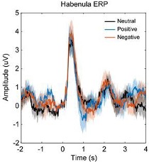
B
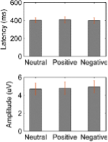
Fig. 3–figure supplement 1. Event-related potential (ERP) in habenula LFP signals in different emotional valence (neutral, positive and negative) conditions. (A) Averaged ERP waveforms across patients for different conditions. (B) Peak latency and amplitude (Mean ± SEM) of the ERP components for different conditions.
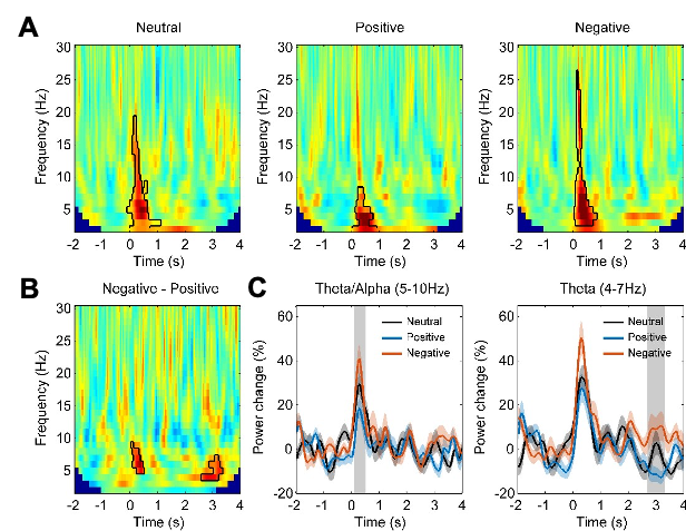
Fig. 3–figure supplement 2. Non-phase-locked activity in different emotional valence (neutral, positive and negative) conditions (N = 18). (A) Time-frequency representation of the power changes relative to pre-stimulus baseline for three conditions. Significant clusters (p < 0.05, non-parametric permutation test) are encircled with a solid black line. (B) Time-frequency representation of the power response difference between negative and positive valence stimuli, showing significant increased activity the theta/alpha band (5-10 Hz) at short latency (100-500 ms) and another increased theta activity (4-7 Hz) at long latencies (2700-3300 ms) with negative stimuli (p < 0.05, non-parametric permutation test). (C) Normalized power of the activities at theta/alpha (5-10 Hz) and theta (4-7 Hz) band over time. Significant difference between the negative and positive valence stimuli is marked by a shadowed bar (p < 0.05, corrected for multiple comparison).
References:
Kalcher J, Pfurtscheller G. Discrimination between phase-locked and non-phase-locked event-related EEG activity. Electroencephalography and Clinical Neurophysiology 1995; 94(5): 381-4.
Cohen MX, Donner TH. Midfrontal conflict-related theta-band power reflects neural oscillations that predict behavior. Journal of Neurophysiology 2013; 110(12): 2752-63.
Figure 4D: can you exclude that the frontal activity is not due to saccade artifacts? Only eye blink artifacts were reduced by the ICA approach. Trials with saccades should be identified in the MEG traces and rejected prior to further analysis.
We understand and appreciate the reviewer’s concern on the source of the activity modulations shown in Fig. 4D. We tried to minimise the eye movement or saccade in the recording by presenting all figures at the centre of the screen, scaling all presented figures to similar size, and presenting a white cross at the centre of the screen preparing the participants for the onset of the stimuli. Despite this, participants my still make eye movements and saccade in the recording. We used ICA to exclude the low frequency large amplitude artefacts which can be related to either eye blink or other large eye movements. However, this may not be able to exclude artefacts related to miniature saccades. As shown in Fig. 4D, on the sensor level, the sensors with significant difference between the negative vs. positive emotional valence condition clustered around frontal cortex, close to the eye area. However, we think this is not dominated by saccades because of the following two reasons:
1.) The power spectrum of the saccadic spike artifact in MEG is characterized by a broadband peak in the gamma band from roughly 30 to 120 Hz (Yuval-Greenberg et al., 2008; Keren et al., 2010). In this study the activity modulation we observed in the frontal sensors are limited to the theta/alpha frequency band, so it is different from the power spectra of the saccadic spike artefact.
2.) The source of the saccadic spike artefacts in MEG measurement tend to be localized to the region of the extraocular muscles of both eyes (Carl et al., 2012).We used beamforming source localisation to identify the source of the activity modulation reported in Fig. 4D. This beamforming analysis identified the source to be in the Broadmann area 9 and 10 (shown in Fig. 5). This excludes the possibility that the activity modulation in the sensor level reported in Fig. 4D is due to saccades. In addition, Broadman area 9 and 10, have previously been associated with emotional stimulus processing (Bermpohl et al., 2006), Broadman area 9 in the left hemisphere has also been used as the target for repetitive transcranial magnetic stimulation (rTMS) as a treatment for drug-resistant depression (Cash et al., 2020). The source localisation results, together with previous literature on the function of the identified source area suggest that the activity modulation we observed in the frontal cortex is very likely to be related to emotional stimuli processing.
References:
Yuval-Greenberg S, Tomer O, Keren AS, Nelken I, Deouell LY. Transient induced gamma-band response in EEG as a manifestation of miniature saccades. Neuron 2008; 58(3): 429-41.
Keren AS, Yuval-Greenberg S, Deouell LY. Saccadic spike potentials in gamma-band EEG: characterization, detection and suppression. NeuroImage 2010; 49(3): 2248-63.
Carl C, Acik A, Konig P, Engel AK, Hipp JF. The saccadic spike artifact in MEG. NeuroImage 2012; 59(2): 1657-67.
Bermpohl F, Pascual-Leone A, Amedi A, Merabet LB, Fregni F, Gaab N, et al. Attentional modulation of emotional stimulus processing: an fMRI study using emotional expectancy. Human Brain Mapping 2006; 27(8): 662-77.
Cash RFH, Weigand A, Zalesky A, Siddiqi SH, Downar J, Fitzgerald PB, et al. Using Brain Imaging to Improve Spatial Targeting of Transcranial Magnetic Stimulation for Depression. Biological Psychiatry 2020.
The coherence modulations in Fig 5 occur quite late in time compared to the power modulations in Fig 3 and 4. When discussing the results (in e.g. the abstract) it reads as if these findings are reflecting the same process. How can the two effect reflect the same process if the timing is so different?
As the reviewer pointed out correctly, the time window where we observed the coherence modulations happened quite late in time compared to the initial power modulations in the frontal cortex and the habenula (Fig. 4). And there was another increase in the theta band activities in the habenula area even later, at around 3 second after stimuli onset when the emotional figure has already disappeared. Emotional response is composed of a number of factors, two of which are the initial reactivity to an emotional stimulus and the subsequent recovery once the stimulus terminates or ceases to be relevant (Schuyler et al., 2014). We think these neural effects we observed in the three different time windows may reflect different underlying processes. We have discussed this in the ‘Discussion’:
"These activity changes at different time windows may reflect the different neuropsychological processes underlying emotion perception including identification and appraisal of emotional material, production of affective states, and autonomic response regulation and recovery (Phillips et al., 2003a). The later effects of increased theta activities in the habenula when the stimuli disappeared were also supported by other literature showing that, there can be prolonged effects of negative stimuli in the neural structure involved in emotional processing (Haas et al., 2008; Puccetti et al., 2021). In particular, greater sustained patterns of brain activity in the medial prefrontal cortex when responding to blocks of negative facial expressions was associated with higher scores of neuroticism across participants (Haas et al., 2008). Slower amygdala recovery from negative images also predicts greater trait neuroticism, lower levels of likability of a set of social stimuli (neutral faces), and declined day-to-day psychological wellbeing (Schuyler et al., 2014; Puccetti et al., 2021)."
References:
Schuyler BS, Kral TR, Jacquart J, Burghy CA, Weng HY, Perlman DM, et al. Temporal dynamics of emotional responding: amygdala recovery predicts emotional traits. Social Cognitive and Affective Neuroscience 2014; 9(2): 176-81.
Phillips ML, Drevets WC, Rauch SL, Lane R. Neurobiology of emotion perception I: The neural basis of normal emotion perception. Biological Psychiatry 2003a; 54(5): 504-14.
Haas BW, Constable RT, Canli T. Stop the sadness: Neuroticism is associated with sustained medial prefrontal cortex response to emotional facial expressions. NeuroImage 2008; 42(1): 385-92.
Puccetti NA, Schaefer SM, van Reekum CM, Ong AD, Almeida DM, Ryff CD, et al. Linking Amygdala Persistence to Real-World Emotional Experience and Psychological Well-Being. Journal of Neuroscience 2021: JN-RM-1637-20.
Be explicit on the degrees of freedom in the statistical tests given that one subject was excluded from some of the tests.
We thank the reviewers for the comment. The number of samples used for each statistics analysis are stated in the title of the figures. We have now also added the degree of freedom in the main text when parametric statistical tests such as t-test or ANOVAs have been used. When permutation tests (which do not have any degrees of freedom associated with it) are used, we have now added the number of samples for the permutation test.
Reviewer #2 (Public Review):
In this study, Huang and colleagues recorded local field potentials from the lateral habenula in patients with psychiatric disorders who recently underwent surgery for deep brain stimulation (DBS). The authors combined these invasive measurements with non-invasive whole-head MEG recordings to study functional connectivity between the habenula and cortical areas. Since the lateral habenula is believed to be involved in the processing of emotions, and negative emotions in particular, the authors investigated whether brain activity in this region is related to emotional valence. They presented pictures inducing negative and positive emotions to the patients and found that theta and alpha activity in the habenula and frontal cortex increases when patients experience negative emotions. Functional connectivity between the habenula and the cortex was likewise increased in this band. The authors conclude that theta/alpha oscillations in the habenula-cortex network are involved in the processing of negative emotions in humans.
Because DBS of the habenula is a new treatment tested in this cohort in the framework of a clinical trial, these are the first data of its kind. Accordingly, they are of high interest to the field. Although the study mostly confirms findings from animal studies rather than bringing up completely new aspects of emotion processing, it certainly closes a knowledge gap.
In terms of community impact, I see the strengths of this paper in basic science rather than the clinical field. The authors demonstrate the involvement of theta oscillations in the habenula-prefrontal cortex network in emotion processing in the human brain. The potential of theta oscillations to serve as a marker in closed-loop DBS, as put forward by the authors, appears less relevant to me at this stage, given that the clinical effects and side-effects of habenula DBS are not known yet.
We thank the reviewers for the favourable comments about the implication of our study in basic science and about the value of our study in closing a knowledge gap. We agree that further studies would be required to make conclusions about the clinical effects and side-effects of habenula DBS.
Detailed comments:
The group-average MEG power spectrum (Fig. 4B) suggests that negative emotions lead to a sustained theta power increase and a similar effect, though possibly masked by a visual ERP, can be seen in the habenula (Fig. 3C). Yet the statistics identify brief elevations of habenula theta power at around 3s (which is very late), a brief elevation of prefrontal power a time 0 or even before (Fig. 4C) and a brief elevation of Habenula-MEG theta coherence around 1 s. It seems possible that this lack of consistency arises from a low signal-to-noise ratio. The data contain only 27 trails per condition on average and are contaminated by artifacts caused by the extension wires.
With regard to the nature of the activity modulation with short latency after stimuli onset: whether this is an ERP or oscillation? We have now investigated this. In summary, by analysing the ERP and removing the influence of the ERP from the total power spectra, we didn’t observe stimulus emotional valence related modulation in the ERP, and the modulation related to emotional valence in the pure induced (non-phase-locked) power spectra was similar to what we have observed in the total power shown in Fig. 3. Therefore, we argue that the theta/alpha increase with negative emotional stimuli we observed in both habenula and prefrontal cortex 0-500 ms after stimuli onset are not dominated by visual or other ERP.
With regard to the signal-to-noise ratio from only 27 trials per condition on average per participant: We have tried to clean the data by removing the trials with obvious artefacts characterised by increased measurements in the time domain over 5 times the standard deviation and increased activities across all frequency bands in the frequency domain. After removing the trials with artefacts, we have 27 trials per condition per subject on average. We agree that 27 trials per condition on average is not a high number, and increasing the number of trials would further increase the signal-to-noise ratio. However, our studies with EEG recordings and LFP recordings from externalised patients have shown that 30 trials was enough to identify reduction in the amplitude of post-movement beta oscillations at the beginning of visuomotor adaption in the motor cortex and STN (Tan et al., 2014a; Tan et al., 2014b). These results of motor error related modulation in the post-movement beta have been repeated by other studies from other groups. In Tan et al. 2014b, with simultaneous EEG and STN LFP measurements and a similar number of trials (around 30), we also quantified the time-course of STN-motor cortex coherence during voluntary movements. This pattern has also been repeated in a separate study from another group with around 50 trials per participant (Talakoub et al., 2016). In addition, similar behavioural paradigm (passive figure viewing paradigm) has been used in two previous studies with LFP recordings from STN from different patient groups (Brucke et al., 2007; Huebl et al., 2014). In both studies, a similar number of trials per condition around 27 was used. The authors have identified meaningful activity modulation in the STN by emotional stimuli. Therefore, we think the number of trials per condition was sufficient to identify emotional valence induced difference in the LFPs in the paradigm.
We agree that the measurement of coherence can be more susceptible to noise and suffer from the reduced signal-to-noise ratio in MEG recording. In Hirschmann et al. 2013, 5 minutes of resting recording and 5 minutes of movement recording from 10 PD patients were used to quantify movement related changes in STN-cortical coherence and how this was modulated by levodopa (Hirschmann et al., 2013). Litvak et al. (2012) have identified movement-related changes in the coherence between STN LFP and motor cortex with recording with simultaneous STN LFP and MEG recordings from 17 PD patients and 20 trials in average per participant per condition (Litvak et al., 2012). With similar methods, van Wijk et al. (2017) used recordings from 9 patients and around on average in 29 trials per hand per condition, and they identified reduced cortico-pallidal coherence in the low-beta decreases during movement (van Wijk et al., 2017). So the trial number per condition participant we used in this study are comparable to previous studies.
The DBS extension wires do reduce signal-to-noise ratio in the MEG recording. therefore the spatiotemporal Signal Space Separation (tSSS) method (Taulu and Simola, 2006) implemented in the MaxFilter software (Elekta Oy, Helsinki, Finland) has been applied in this study to suppress strong magnetic artifacts caused by extension wires. This method has been proved to work well in de-noising the magnetic artifacts and movement artifacts in MEG data in our previous studies (Cao et al., 2019; Cao et al., 2020). In addition, the beamforming method proposed by several studies (Litvak et al., 2010; Hirschmann et al., 2011; Litvak et al., 2011) has been used in this study. In Litvak et al., 2010, the artifacts caused by DBS extension wires was detailed described and the beamforming was demonstrated to effectively suppress artifacts and thereby enable both localization of cortical sources coherent with the deep brain nucleus. We have now added more details and these references about the data cleaning and the beamforming method in the main text. With the beamforming method, we did observe the standard movement-related modulation in the beta frequency band in the motor cortex with 9 trials of figure pressing movements, shown in the following figure for one patient as an example (Figure 5–figure supplement 1). This suggests that the beamforming method did work well to suppress the artefacts and help to localise the source with a low number of trials. The figure on movement-related modulation in the motor cortex in the MEG signals have now been added as a supplementary figure to demonstrate the effect of the beamforming.
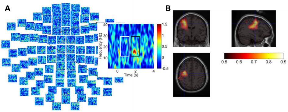
Figure 5–figure supplement 1. (A) Time-frequency maps of MEG activity for right hand button press at sensor level from one participant (Case 8). (B) DICS beamforming source reconstruction of the areas with movement-related oscillation changes in the range of 12-30 Hz. The peak power was located in the left M1 area, MNI coordinate [-37, -12, 43].
References:
Tan H, Jenkinson N, Brown P. Dynamic neural correlates of motor error monitoring and adaptation during trial-to-trial learning. Journal of Neuroscience 2014a; 34(16): 5678-88.
Tan H, Zavala B, Pogosyan A, Ashkan K, Zrinzo L, Foltynie T, et al. Human subthalamic nucleus in movement error detection and its evaluation during visuomotor adaptation. Journal of Neuroscience 2014b; 34(50): 16744-54.
Talakoub O, Neagu B, Udupa K, Tsang E, Chen R, Popovic MR, et al. Time-course of coherence in the human basal ganglia during voluntary movements. Scientific Reports 2016; 6: 34930.
Brucke C, Kupsch A, Schneider GH, Hariz MI, Nuttin B, Kopp U, et al. The subthalamic region is activated during valence-related emotional processing in patients with Parkinson's disease. European Journal of Neuroscience 2007; 26(3): 767-74.
Huebl J, Spitzer B, Brucke C, Schonecker T, Kupsch A, Alesch F, et al. Oscillatory subthalamic nucleus activity is modulated by dopamine during emotional processing in Parkinson's disease. Cortex 2014; 60: 69-81.
Hirschmann J, Ozkurt TE, Butz M, Homburger M, Elben S, Hartmann CJ, et al. Differential modulation of STN-cortical and cortico-muscular coherence by movement and levodopa in Parkinson's disease. NeuroImage 2013; 68: 203-13.
Litvak V, Eusebio A, Jha A, Oostenveld R, Barnes G, Foltynie T, et al. Movement-related changes in local and long-range synchronization in Parkinson's disease revealed by simultaneous magnetoencephalography and intracranial recordings. Journal of Neuroscience 2012; 32(31): 10541-53.
van Wijk BCM, Neumann WJ, Schneider GH, Sander TH, Litvak V, Kuhn AA. Low-beta cortico-pallidal coherence decreases during movement and correlates with overall reaction time. NeuroImage 2017; 159: 1-8.
Taulu S, Simola J. Spatiotemporal signal space separation method for rejecting nearby interference in MEG measurements. Physics in Medicine and Biology 2006; 51(7): 1759-68.
Cao C, Huang P, Wang T, Zhan S, Liu W, Pan Y, et al. Cortico-subthalamic Coherence in a Patient With Dystonia Induced by Chorea-Acanthocytosis: A Case Report. Frontiers in Human Neuroscience 2019; 13: 163.
Cao C, Li D, Zhan S, Zhang C, Sun B, Litvak V. L-dopa treatment increases oscillatory power in the motor cortex of Parkinson's disease patients. NeuroImage Clinical 2020; 26: 102255.
Litvak V, Eusebio A, Jha A, Oostenveld R, Barnes GR, Penny WD, et al. Optimized beamforming for simultaneous MEG and intracranial local field potential recordings in deep brain stimulation patients. NeuroImage 2010; 50(4): 1578-88.
Litvak V, Jha A, Eusebio A, Oostenveld R, Foltynie T, Limousin P, et al. Resting oscillatory cortico-subthalamic connectivity in patients with Parkinson's disease. Brain 2011; 134(Pt 2): 359-74.
Hirschmann J, Ozkurt TE, Butz M, Homburger M, Elben S, Hartmann CJ, et al. Distinct oscillatory STN-cortical loops revealed by simultaneous MEG and local field potential recordings in patients with Parkinson's disease. NeuroImage 2011; 55(3): 1159-68.
I doubt that the correlation between habenula power and habenula-MEG coherence (Fig. 6C) is informative of emotion processing. First, power and coherence in close-by time windows are likely to to be correlated irrespective of the task/stimuli. Second, if meaningful, one would expect the strongest correlation for the negative condition, as this is the only condition with an increase of theta coherence and a subsequent increase of theta power in the habenula. This, however, does not appear to be the case.
The authors included the factors valence and arousal in their linear model and found that only valence correlated with electrophysiological effects. I suspect that arousal and valence scores are highly correlated. When fed with informative yet highly correlated variables, the significance of individual input variables becomes difficult to assess in many statistical models. Hence, I am not convinced that valence matters but arousal not.
For the correlation shown in Fig. 6C, we used a linear mixed-effect modelling (‘fitlme’ in Matlab) with different recorded subjects as random effects to investigate the correlations between the habenula power and habenula-MEG coherence at an earlier window, while considering all trials together. Therefore the reported value in the main text and in the figure (k = 0.2434 ± 0.1031, p = 0.0226, R2 = 0.104) show the within subjects correlation that are consistent across all measured subjects. The correlation is likely to be mediated by emotional valence condition, as negative emotional stimuli tend to be associated with both high habenula-MEG coherence and high theta power in the later time window tend to happen in the trials with.
The arousal scores are significantly different for the three valence conditions as shown in Fig. 1B. However, the arousal scores and the valence scores are not monotonically correlated, as shown in the following figure (Fig. S2). The emotional neutral figures have the lowest arousal value, but have the valence value sitting between the negative figures and the positive figures. We have now added the following sentence in the main text:
"This nonlinear and non-monotonic relationship between arousal scores and the emotional valence scores allowed us to differentiate the effect of the valence from arousal."
Table 2 in the main text show the results of the linear mixed-effect modelling with the neural signal as the dependent variable and the valence and arousal scores as independent variables. Because of the non-linear and non-monotonic relationship between the valence and arousal scores, we think the significance of individual input variables is valid in this statistical model. We have now added a new figure (shown below, Fig. 7) with scatter plots showing the relationship between the electrophysiological signal and the arousal and emotional valence scores separately using Spearman’s partial correlation analysis. In each scatter plot, each dot indicates the average measurement from one participant in one emotional valence condition. As shown in the following figure, the electrophysiological measurements linearly correlated with the valence score, but not with the arousal scores. However, the statistics reported in this figure considered all the dots together. The linear mixed effect modelling taking into account the interdependency of the measurements from the same participant. So the results reported in the main text using linear mixed effect modelling are statistically more valid, but supplementary figure here below illustrate the relationship.
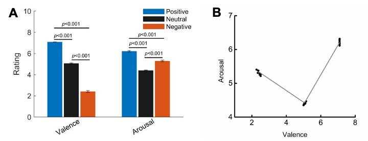
Figure S2. Averaged valence and arousal ratings (mean ± SD) for figures of the three emotional condition. (B) Scatter plots showing the relationship between arousal and valence scores for each emotional condition for each participant.
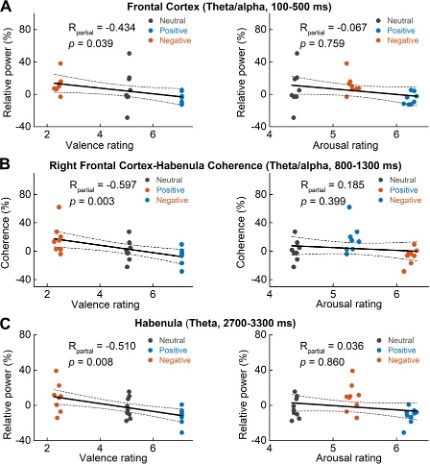
Figure 7. Scatter plots showing how early theta/alpha band power increase in the frontal cortex (A), theta/alpha band frontal cortex-habenula coherence (B) and theta band power increase in habenula stimuli (C) changed with emotional valence (left column) and arousal (right column). Each dot shows the average of one participant in each categorical valence condition, which are also the source data of the multilevel modelling results presented in Table 2. The R and p value in the figure are the results of partial correlation considering all data points together.
Page 8: "The time-varying coherence was calculated for each trial". This is confusing because coherence quantifies the stability of a phase difference over time, i.e. it is a temporal average, not defined for individual trials. It has also been used to describe the phase difference stability over trials rather than time, and I assume this is the method applied here. Typically, the greatest coherence values coincide with event-related power increases, which is why I am surprised to see maximum coherence at 1s rather than immediately post-stimulus.
We thank the reviewer for pointing out this incorrect description. As the reviewer pointed out correctly, the method we used describe the phase difference stability over trials rather than time. We have now clarified how coherence was calculated and added more details in the methods:
"The time-varying cross trial coherence between each MEG sensor and the habenula LFP was first calculated for each emotional valence condition. For this, time-frequency auto- and cross-spectral densities in the theta/alpha frequency band (5-10 Hz) between the habenula LFP and each MEG channel at sensor level were calculated using the wavelet transform-based approach from -2000 to 4000 ms for each trial with 1 Hz steps using the Morlet wavelet and cycle number of 6. Cross-trial coherence spectra for each LFP-MEG channel combination was calculated for each emotional valence condition for each habenula using the function ‘ft_connectivityanalysis’ in Fieldtrip (version 20170628). Stimulus-related changes in coherence were assessed by expressing the time-resolved coherence spectra as a percentage change compared to the average value in the -2000 to -200 ms (pre-stimulus) time window for each frequency."
In the Morlet wavelet analysis we used here, the cycle number (C) determines the temporal resolution and frequency resolution for each frequency (F). The spectral bandwidth at a given frequency F is equal to 2F/C while the wavelet duration is equal to C/F/pi. We used a cycle number of 6. For theta band activities around 5 Hz, we will have the spectral bandwidth of 25/6 = 1.7 Hz and the wavelet duration of 6/5/pi = 0.38s = 380ms.
As the reviewer noticed, we observed increased activities across a wide frequency band in both habenula and the prefrontal cortex within 500 ms after stimuli onset. But the increase of cross-trial coherence starts at around 300 ms. The increase of coherence in a time window without increase of power in either of the two structures indicates a phase difference stability across trials in the oscillatory activities from the two regions, and this phase difference stability across trials was not secondary to power increase.
Reviewer #3 (Public Review):
This paper describes the oscillatory activity of the habenula using local field potentials, both within the region and, through the use of MEG, in connection to the prefrontal cortex. The characteristics of this activity were found to vary with the emotional valence but not with arousal. Sheding light on this is relevant, because the habenula is a promising target for deep brain stimulation.
In general, because I am not much on top of the literature on the habenula, I find difficult to judge about the novelty and the impact of this study. What I can say is that I do find the paper is well-written and very clear; and the methods, although quite basic (which is not bad), are sound and rigourous.
We thank the reviewer for the positive comments about the potential implication of our study and on the methods we used.
On the less positive side, even though I am aware that in this type of studies it is difficult to have high N, the very low N in this case makes me worry about the robustness and replicability of the results. I'm sure I have missed it and it's specified somewhere, but why is N different for the different figures? Is it because only 8 people had MEG? The number of trials seems also a somewhat low. Therefore, I feel the authors perhaps need to make an effort to make up for the short number of subjects in order to add confidence to the results. I would strongly recommend to bootstrap the statistical analysis and extract non-parametric confidence intervals instead of showing parametric standard errors whenever is appropriate. When doing that, it must be taken into account that each two of the habenula belong to the same person; i.e. one bootstraps the subjects not the habenula.
We do understand and appreciate the concern of the reviewer on the low sample numbers due to the strict recruitment criteria for this very early stage clinical trial: 9 patients for bilateral habenula LFPs, and 8 patients with good quality MEGs. Some information to justify the number of trials per condition for each participant has been provided in the reply to the Detailed Comments 1 from Reviewer 2. The sample number used in each analysis was included in the figures and in the main text.
We have used non-parametric cluster-based permutation approach (Maris and Oostenveld, 2007) for all the main results as shown in Fig. 3-5. Once the clusters (time window and frequency band) with significant differences for different emotional valence conditions have been identified, parametric statistical test was applied to the average values of the clusters to show the direction of the difference. These parametric statistics are secondary to the main non-parametric permutation test.
In addition, the DICS beamforming method was applied to localize cortical sources exhibiting stimuli-related power changes and cortical sources coherent with deep brain LFPs for each subject for positive and negative emotional valence conditions respectively. After source analysis, source statistics over subjects was performed. Non-parametric permutation testing with or without cluster-based correction for multiple comparisons was applied to statistically quantify the differences in cortical power source or coherence source between negative and positive emotional stimuli.
References:
Maris E, Oostenveld R. Nonparametric statistical testing of EEG- and MEG-data. Journal of Neuroscience Methods 2007; 164(1): 177-90.
Related to this point, the results in Figure 6 seem quite noisy, because interactions (i.e. coherence) are harder to estimate and N is low. For example, I have to make an effort of optimism to believe that Fig 6A is not just noise, and the result in Fig 6C is also a bit weak and perhaps driven by the blue point at the bottom. My read is that the authors didn't do permutation testing here, and just a parametric linear-mixed effect testing. I believe the authors should embed this into permutation testing to make sure that the extremes are not driving the current p-value.
We have now quantified the coherence between frontal cortex-habenula and occipital cortex-habenula separately (please see more details in the reply to Reviewer 2 (Recommendations for the authors 6). The new analysis showed that the increase in the theta/alpha band coherence around 1 s after the negative stimuli was only observed between prefrontal cortex-habenula and not between occipital cortex-habenula. This supports the argument that Fig. 6A is not just noise.
Reviewer #1:
Köster and colleagues present a brief report in which they study in 9 month-old babies the electrophysiological responses to expected and unexpected events. The major finding is that in addition to a known ERP response, an NC present between 400-600 ms, they observe a differential effect in theta oscillations. The latter is a novel result and it is linked to the known properties of theta oscillations in learning. This is a nice study, with novel results and well presented. My major reservation however concerns the push the authors make for the novelty of the results and their interpretation as reflecting brain dynamics and rhythms. The reason for that is, that any ERP, passed through the lens of a wavelet/FFT etc, will yield a response at a particular frequency. This is especially the case for families of ERP responses related to unexpected event e.g., MMR, and NC, etc. For which there is plenty of literature linking them to responses to surprising event, and in particular in babies; and which given their timing will be reflected in delta/theta oscillations. The reason why I am pressing on this issue, is because there is an old, but still ongoing debate attempting to dissociate intrinsic brain dynamics from simple event related responses. This is by no means trivial and I certainly do not expect the authors to resolve it, yet I would expect the authors to be careful in their interpretation, to warn the reader that the result could just reflect the known ERP, to avoid introducing confusion in the field.
We would like to thank the author for highlighting the novelty of the results. Critically, there is one fundamental difference in investigating the ERP response and the trial-wise oscillatory power, which we have done in the present analysis: when looking at the evoked oscillatory response (i.e., the TF characteristics of the ERP), the signal is averaged over trials first and then subjected to a wavelet transform. However, when looking at the ongoing (or total) oscillatory response, the wavelet transform is applied at the level of the single trial, before the TF response of the single trials is averaged across the trials of one condition trials (for a classical illustration, see Tallon-Baudry & Bertrand, 1999; TICS, Box 2). We have now made this distinction more salient throughout the manuscript.
In the present study, the results did not suggest a relation between the ERP and the ongoing theta activity, because the topography, temporal evolution, and polarity of the ERP and the theta response were very dissimilar: Looking at Figure 2 (A and B) and Figure 3 (B and C), the Nc peaks at central electrodes, but the theta response is more distributed, and the expected versus unexpected difference was specific for the .4 to .6 s time window, but the theta difference lasted the whole trial. Furthermore, the NC was higher for expected versus unexpected, which should (due to the low frequency) rather lead to a higher theta power for unexpected, in contrast to expected events for the time frequency analysis for the Nc. To verify this intuition, we now ran a wavelet analysis on the evoked response (i.e., the ERP) and, for a direct comparison, also plotted the ongoing oscillatory response for the central electrodes (see Additional Figure 1). These additional analyses nicely illustrate that the trial-wise theta response provides a fundamentally different approach to analyze oscillatory brain dynamics.
Because this is likely of interest to many readers, we also report the results of the wavelet analysis of the ERP versus the analysis of the ongoing theta activity at central electrodes and the corresponding statistics in the result section, and have also included the Additional Figure in the supplementary materials, as Figure S2.
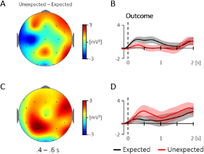
Additional Figure 1. Comparison of the topography and time course for the 4 – 5 Hz activity for the evoked (A, B) and the ongoing (C, D) oscillatory response at central electrodes (400 – 600 ms; Cz, C3, C4; baseline: -100 – 0 ms). (A) Topography for the difference between unexpected and expected events in the evoked oscillatory response. (B) The corresponding time course at central electrodes, which did not reveal a significant difference between 400 – 600 ms, t(35) = 1.57, p = .126. (C) Topography for the same contrast in the ongoing oscillatory response and (D) the corresponding time course at central electrodes, which did likewise not reveal a significant difference between 400 – 600 ms, t(35) = -1.26, p = .218. The condition effects (unexpected - expected) were not correlated between the evoked and the ongoing response, r = .23, p = .169.
A second aspect that I would like the authors to comment on is the power of the experimental design to measure surprise. From the methods, I gathered that the same stimulus materials and with the same frequency were presented as expected and unexpected endings. If that is the case, what is the measure of surprise? For once the same materials are shown causing habituation and reducing novelty and second the experiment introduces a long-term expectation of a 50:50 proportion of expected/unexpected events. I might be missing something here, which is likely as the methods are quite sparse in the description of what was actually done.
We have used 4 different stimuli types (variants) in each of the 4 different domains, with either an expected or unexpected outcome. This resulted in 32 distinct stimulus sequences, which we presented twice, resulting in (up to) 64 trials. We have now described this approach and design in more detail and have also included all stimuli as supplementary material (Figure S1). In particular, we have used multiple types in each domain to reduce potential habituation or expectation effects. Still, we agree that one difficulty may be that, over time, infants got used to the fact that expected and unexpected outcomes were to be similarly “expected” (i.e., 50:50). However, if this was the case it would have resulted in a reduction (or disappearance) of the condition effect, and would thus also reduce the condition difference that we found, rather than providing an alternative explanation. We now included this consideration in the method section (p. 7).
Two more comments concerning the analysis choices:
1) The statistics for the ERP and the TF could be reported using a cluster size correction. These are well established statistical methods in the field which would enable to identify the time window/topography that maximally distinguished between the expected and the unexpected condition both for ERP and TF. Along the same lines, the authors could report the spatial correlation of the ERP/TF effects.
For the ERP analysis we used the standard electrodes typically analyzed for the Nc in order to replicate effects found in former research (Langeloh et al., 2020; see also, Kayhan et al., 2019; Reynolds and Richards, 2005; Webb et al., 2005). For the TF analyses we used the most conservative criterion, namely all scalp recorded electrodes and the whole time window from 0 to 2000 ms, such that we did not make any choice regarding time window or the electrodes (i.e., which could be corrected for against other choices). We have now made those choices clearer in the method section, and why we think that, under these condition a multiple comparison correction is not needed/applicable (p. 10). Regarding the spatial correlation of the ERP and TF effects, we explained in response to the first comment the very different nature of the TF decomposition of the ERP and ongoing oscillatory activity and also that these were found to be interdependent (i.e., uncorrelated). We hope that with the additional analysis included in response to this comment that this difference is much clearer now.
2) While I can see the reason why the authors chose to keep the baseline the same between the ERP and the TF analysis, for time frequency analysis it would be advisable to use a baseline amounting to a comparable time to the frequency of interest; and to use a period that does not encroach in the period of interest i.e., with a wavelet = 7 and a baseline -100:0 the authors are well into the period of interested.
The difficulty in choosing the baseline in the present study was two-fold. First, we were interested in the ERP and the change in neural oscillations upon the onset of an outcome picture within a continuous presentation of pictures, forming a sequence. Second, we wanted to use a similar baseline for both analyses, to make them comparable. Because the second picture (the picture before the outcome picture) also elicited both an ERP and an oscillatory response at ~ 4 Hz (see Additional Figure 2), we choose a baseline just before the onset of the outcome stimulus, from -100 to 0 ms. Also we agree that the possibility to take a longer and earlier baseline, in particular for the TF results would have been favorable, but still consider that the -100 to 0 ms is still the best choice for the present analysis. Notably, because we found an increase in theta oscillations and the critical difference relies on a higher theta rhythm in one compared to the other condition, the effects of the increase in theta, if they effected the baseline, this effect would counteract rather than increase the current effect. We now explain this choice in more detail (p.10).
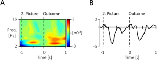
Additional Figure 1. Display of the grand mean signals prior to the -100 to 0 baseline and outcome stimulus. (A) The time-frequency response across all scalp-recorded electrodes, as well as (B) the ERP at the central electrodes (Cz, C3, C4) across both conditions show a similar response to the 2. picture like the outcome picture. Thus a baseline just prior to the stimulus of interest was chosen, consistent for both analyses.
Reviewer #2:
The manuscript reports increases in theta power and lower NC amplitude in response to unexpected (vs. expected) events in 9-month-olds. The authors state that the observed increase in theta power is significant because it is in line with an existing theory that the theta rhythm is involved in learning in mammals. The topic is timely, the results are novel, the sample size is solid, the methods are sound as far as I can tell, and the use of event types spanning multiple domains (e.g. action, number, solidity) is a strength. The manuscript is short, well-written, and easy to follow.
1) The current version of the manuscript states that the reported findings demonstrate that the theta rhythm is involved in processing of prediction error and supports the processing of unexpected events in 9-month-old infants. However, what is strictly shown is that watching at least some types of unexpected events enhance theta rhythm in 9-month-old infants, i.e. an increase in the theta rhythm is associated with processing unexpected events in infants, which suggests that an increase in the theta rhythm is a possible neural correlate of prediction error in this age range. While the present novel findings are certainly suggestive, more data and/or analyses would be needed to corroborate/confirm the role of the observed infant theta rhythm in processing prediction error, or document whether and how this increase in the theta rhythm supports the processing of unexpected events in infants. (As an example, since eye-tracking data were collected, are trial-by-trial variations in theta power increases to unexpected outcomes related to how long individual infants looked to the unexpected outcome pictures?) If it is not possible to further confirm/corroborate the role of the theta rhythm with this dataset, then the discussion, abstract, and title should be revised to more closely reflect what the current data shows (as the wording of the conclusion currently does), and clarify how future research may test the hypothesis that the infant theta rhythm directly supports the processing of prediction error in response to unexpected events.
We would like to thank the reviewer for acknowledging the merit of the present research.
On the one hand, we have revised our manuscript and are now somewhat more careful with our conclusion, in particular with regard to the refinement of basic expectations. On the other hand, we consider the concept of “violation to expectation” (VOE), which is one of the most widely used concepts in infancy research, very closely linked to the concept of a prediction error processing, namely a predictive model is violated. In particular, we have made this conceptual link in a recent theoretical paper (Köster et al., 2020), and based on former theoretical considerations about the link between these two concepts (e.g., see Schubotz 2015; Prediction and Expectation). In particular, in the present study we used a set of four different domains of violation of expectation paradigms, which are among the best established domains of infants core knowledge (e.g., action, solidity, cohesion, number; cf. Spelke & Kinzler, 2007). It was our specific goal not to replicate, for another time, that infants possess expectations (i.e., make predictions) in these domains, but to “flip the coin around” and investigate infants’ prediction error more generally, independent of the specific domain. We have now made the conceptual link between VOE and prediction error processing more explicit in the introduction of the manuscript and also emphasize that we choose a variety of domains to obtain a more general neural marker for infant processing of prediction errors.
Having said this, indeed, we planned to assess and compare both infants gaze behavior and EEG response. Unfortunately, this was not very successful and the concurrent recording only worked for a limited number of infants and trials. This led us to the decision to make the eye-tracking study a companion study and to collect more eye-tracking data in an independent sample of infants after the EEG assessment was completed, such that a match between the two measures was not feasible. We now make this choice more explicit in the method section (p. 7). In addition, contrary to our basic assumption we did not find an effect in the looking time measure. Namely, there was no difference between expected and unexpected outcomes. We assume that this is due to the specificities of the current design that was rather optimized for EEG assessments: We used a high number of repetitions (64), with highly variable domains (4), and restricted the time window for potential looking time effects to 5 seconds, which is highly uncommon in the field and therefore not directly comparable with former studies.
Finally, besides the ample evidence from former studies using VOE paradigms, if it were not the unexpected vs. expected (i.e., unpredicted vs. predicted) condition contrast which explains the differences we found in the ERP and the theta response, there would need to be an alternative explanation for the differential responses in the EEG, which produce the hypothesized effects. (Please also note that there are many studies relying their VOE assumption on ERPs alone, here we have two independent measures suggesting that infants discriminated between those conditions.)
2) The current version of the manuscript states "The ERP effect was somewhat consistent across conditions, but the effect was mainly driven by the differences between expected and unexpected events in the action and the number domain (Figure S1). The results were more consistent across domains for the condition difference in the 4 - 5 Hz activity, with a peak in the unexpected-expected difference falling in the 4 - 5 Hz range across all electrodes (Figure S2)". However, the similarity/dissimilarity of NC and theta activity responses across domains was not quantified or tested. Looking at Figures S1 and S2, it is not that obvious to me that theta responses were more consistent across domains than NC responses. I understand that there were too few trials to formally test for any effect of domain (action, number, solidity, cohesion) on NC and theta responses, either alone or in interaction with outcome (expected, unexpected). It may still be possible to test for correlations of the topography and time-course of the individual average unexpected-expected difference in NC and theta responses across domains at the group level, or to test for an effect of outcome (expected, unexpected) in individual domains for subgroups of infants who contributed enough trials. Alternatively, claims of consistency across domains may be altered throughout, in which case the inability to test whether the theta and/or NC signatures of unexpected event processing found are consistent across domains (vs. driven by some domains) should be acknowledged as a limitation of the present study.
We agree that this statement rather reflected our intuition and would not surpass statistical analysis given the low number of trials. So we are happy to refrain from this claim and simply refer to the supplementary material for the interested reader and also mention this as a perspective for future research in the discussion (p. 12; p. 15).
As outlined in our previous response, it was also not our goal to draw conclusions about each single domain, but rather to present a diversity of stimulus types from different core knowledge domains to gain a more generalized neural marker for infants’ processing of unexpected, i.e., unpredicted events.
Reviewer #3:
General assessment:
In this manuscript, the authors bring up a contemporary and relevant topic in the field, i.e. theta rhythm as a potential biomarker for prediction error in infancy. Currently, the literature is rich on discussions about how, and why, theta oscillations in infancy implement the different cognitive processes to which they have been linked. Investigating the research questions presented in this manuscript could therefore contribute to fill these gaps and improve our understanding of infants' neural oscillations and learning mechanisms. While we appreciate the motivation behind the study and the potential in the authors' research aim, we find that the experimental design, analyses and conclusions based on the results that can be drawn thereafter, lack sufficient novelty and are partly problematic in their description and implementation. Below, we list our major concerns in more detail, and make suggestions for improvements of the current analyses and manuscript.
Summary of major concerns:
1) Novelty:
(a) It is unclear how the study differs from Berger et al., 2006 apart from additional conditions. Please describe this study in more detail and how your study extends beyond it.
We would like to thank the reviewers for emphasizing the timeliness and relevance of the study.
The critical difference between the present study and the study by Berger et al. 2006 was that the authors applied, as far as we understand this from Figure 4 and the method section of their study, the wavelet analysis to the ERP signal. In contrast, in the present study, we applied the wavelet analysis at the level of single trials. We now explain the difference between the two signals in more detail in the revised manuscript and also included an additional comparison between the evoked (i.e., ERP) and the ongoing (i.e., total) oscillatory response (for more details, please see the first response to the first comment of reviewer 1).
(b) Seemingly innovative aspects (as listed below), which could make the study stand out among previous literature, but are ultimately not examined. Consequently, it is also not clear why they are included.
-Relation between Nc component and theta.
-Consistency of the effect across different core knowledge domains.
-Consistency of the effect across the social and non-social domains.
-Link between infants looking at time behavior and theta.
We are thankful for these suggestions, which are closely related to the points raised by reviewer 1 and 2. With regard to the relation between the Nc and the theta response, we have now included a direct comparison of these signals (see Additional Figure 1, i.e., novel Figure S2; for details, please see the first response to the first comment of reviewer 1). Regarding the consistency of effects across domains, we have explained in response to point 1 by reviewer 2 that this was not the specific purpose of the present study, but we aimed at using a diversity of VOE stimuli to obtain a more general neural signature for infants’ prediction error processing, and explain this in more detail in the revised manuscript. Having said this, we agree that the question of consistency of effects between conditions is highly interesting, but we would not consider the data robust enough to confidently test these differences given the limited number of trials available per stimulus category. We now discuss this as a direction for future research (p. 15). Finally, we also agree with regard to the link between looking times and the theta rhythm. As also outlined in response to point 1 by reviewer 2 (paragraph 2), we initially had this plan, but did not succeed in obtaining a satisfactory number of trials in the dual recording of EEG and eye-tracking, which made us change these plans. This is now explained in detail in the method section (p. 7).
(c) The reason to expect (or not) a difference at this age, compared to what is known from adult neural processing, is not adequately explained.
-Potentially because of neural generators in mid/pre-frontal cortex? See Lines 144-146.
The overall aim of the present study was to identify the neural signature for prediction error processing in the infant brain, which has, to the best of our knowledge, not been done this explicitly and with a focus on the ongoing theta activity and across a variety of violations in infants’ core knowledge domains. Because we did not expect a specific topography of this effect, in particular across multiple domains, we included all electrodes in the analyses. We have now clarified this in the method section (p. 10).
(d) The study is not sufficiently embedded in previous developmental literature on the functionality of theta. That is, consider theta's role in error processing, but also the increase of theta over time of an experiment and it's link to cognitive development. See, for example: Braithwaite et al., 2020; Conejero et al., 2018; Adam et al., 2020.
We are thankful that the reviewer indicated these works and have now included them in the introduction and discussion. Closest to the present study is the study by Conejero et al., 2018. However, this study is also based on theta analyses of the ERP, not of the ongoing oscillatory response and it includes considerably older infants (i.e., 16-month-olds instead of 9-month-olds as in the present study).
2) Methodology:
(a) Design: It is unclear what exactly a testing session entails.
-Was the outcome picture always presented for 5secs? The methods section suggests that, but the introduction of the design and Figure 1 do not. This might be misleading. Please change in Figure 1 to 5sec if applicable.
Yes, the final images were shown for 5s in order to simultaneously assess infants’ looking times. However, we included trials in the EEG analysis if infants looked for 2s, so this is the more relevant info for the analysis. We now clarified this in the method section (p. 7) and have also added this info in the figure caption.
-Were infants' eye-movements tracked simultaneously to the EEG recording? If so, please present findings on their looking time and (if possible) pupil size. Also examine the relation to theta power. This would enhance the novelty and tie these findings to the larger looking time literature that the authors refer to in their introduction.
Yes, in response to the second reviewer (comment 1) we explained in more detail why the joint analysis of the EEG and looking time data was not possible: We planned to assess both, infants gaze behavior and EEG response. Unfortunately, this was not very successful and the dual recording only worked for a few infants and trials. This led us to collect more eye-tracking data after the EEG assessment was completed, such that a match between the two measures was not feasible. We now clarified this in the method section (p. 7).
(b) Analysis:
-In terms of extracting theta power information: The baseline of 100ms is extremely short for a comparison in the frequency domain, since it does not even contain half a cycle of the frequency of interest, i.e. 4Hz. We appreciate the thought to keep the baseline the same as in the ERP analysis (which currently is hardly focused on in the manuscript), but it appears problematic for the theta analysis. Also, if we understand the spectral analysis correctly, the window the authors are using to estimate their spectral estimates is largely overlapping between baseline and experimental window. The question arises whether a baseline is even needed here, or if a direct contrast between conditions might be better suited.
Please see our explanation about the choice of the baseline in our response to reviewer 1, comment 2. Because our stimulus sequences were highly variable, likely leading to highly variable overall theta activity, and our specific interest was in the change in theta activity upon the onset of the unexpected versus unpredicted outcome, we still consider it useful to take a baseline here. Also because this makes the study more closely comparable to the existing literature. We now clarified this in the method section (p. 9)
-In terms of statistical testing
-It appears that the authors choose the frequency band that will be entered in the statistical analysis from visual inspection of the differences between conditions. They write: "we found the strongest difference between 4 - 5 Hz (see lower panel of Figure 3). Therefore, and because this is the first study of this kind, we analyzed this frequency range." ll. 277-279). This approach seems extremely problematic since it poses a high risk for 'double-dipping'. This is crucial and needs to be addressed. For instance, the authors could run non-parametric permutation tests on the time-frequency domain using FDR correction or cluster-based permutation tests on the topography.
-Lack of examining time- / topographic specificity.
Please also note the sentence before this citation, which states our initial hypothesis: “While our initial proposal was to look at the difference in the 4 Hz theta rhythm between conditions (Köster et al., 2019), we found the strongest difference between 4 – 5 Hz (see lower panel of Figure 3).” Note that the hypothesis of 4 Hz can be clearly derived from our 2019 study. We would maintain that the center frequency we took for the analysis 4.5Hz (i.e., 4 – 5Hz) is very close to this original hypothesis and, considering that we applied a novel design and analyses in very young infants, could indeed hardly have fallen more closely to this initial proposal. The frequency choice is also underlined, as the reviewer remarks, by the consistency of this peak across domains, peaking at 4Hz (cohesion), 4.5Hz (action), and 5Hz (solidity, number). Importantly, please note that we have chosen the electrodes and time window very conservatively, namely by including the whole time period and all electrodes, which we now explain in more detail on p. 10. Please also see our response to reviewer 1, comment “1)”.
3) Interpretation of results:
(a) The authors interpret the descriptive findings of Figure S1 as illustration of the consistency of the results across the four knowledge domains. While we would partly agree with this interpretation based on column A of that figure (even though also there the peak shifts between domains), columns B and C do not picture a consistent pattern of data. That is, the topography appears very different between domains and so does the temporal course of the 4-5Hz power, with only showing higher power in the action and number domain, not in the other two. Since none of these data were compared statistically, any interpretation remains descriptive. Yet, we would like to invite the authors to critically reconsider their interpretation. You also might want to consider adding domain (action, number etc.) as a covariate to your statistical model.
We agree with the reviewers (reviewer 2 and reviewer 3) that our initial interpretation of the data regarding the consistency of effects across domains may have been too strong. Thus, in the revised version of the manuscript, we do not state that the TF analysis revealed more consistent results. Given that the analysis was based on a different subsample and highly variable in trial numbers, we did not enter them as a covariate in the statistical model.
Note: This response was posted by the corresponding author to Review Commons. The content has not been altered except for formatting.
Learn more at Review Commons
Manuscript number: RC-2025-03220
Corresponding author(s): Ryusuke Niwa, Yuko Shimada-Niwa, and Wei Sun
Dear Editors,
We are pleased to submit our revised manuscript of RC-2025-03220R. The reviewers’ comments from Review Commons are presented in italic.
For submission of our current revised manuscript, we provide two Word files, which are the “clean” and “Track-and-Change” files. Page and line numbers described below correspond to those of the “clean” file. The “Track-and-Change” file might be helpful for Reviewers to find what we have changed for the current revision.
We hope that the revised version is now suitable for the next stage of evaluation.
Sincerely,
Ryusuke Niwa, Yuko Shimada-Niwa, and Wei Sun
We sincerely thank the reviewers for their thoughtful feedback on our initial submission. Experiments that we will conduct and the revisions on the manuscript that have already been incorporated are detailed below in the point-by-point response. For this revised submission, two versions of the manuscript are provided: a clean copy and a tracked-changes file. Page and line numbers mentioned below refer to the clean version, while the tracked-changes file is intended to help reviewers easily identify the revisions made.
In preparing the revision plan, we have included additional data, some of which were generated in collaboration with new contributors. Accordingly, we would like to propose adding Yuichi Shichino and Shintaro Iwasaki as co-authors to acknowledge their contributions.
__
- Also, the authors show that two different RNAi lines for NudC give the same defects - it would be good to know if the RNAi lines target the same or different sequences in the NudC transcripts. Alternatively, it would be equally good to show that trans-allelic combinations of NudC mutants have the same defects in the prothoracic glands and the salivary glands as the RNAi. Instead, they examine only overall body size, developmental delays and lethality in the trans-hetero allelic NudC mutants.
Author response:
In response to the second part of the criticism, we will further validate the observed phenotypes by examining tissue and nuclear size, chromosomal structure, and the levels of Fibrillarin and RpS6 proteins in the prothoracic glands and salivary glands of NudC mutants.
__
- It would be quite helpful to characterize the "5 blob" and "shortened polytene chromosome arm" defects shown in Figure 2 and Figure 6. Are these partially polytenized chromosomes or are large sections of the chromosomes missing or just underreplicated? What do the chromosomes look like if you lyse the nuclei, spread the chromosomes and stain with DAPI or Hoechst - this is a pretty standard practice and would reveal much more about the structure of the polytene chromosomes.
Author response:
To address these structural concerns more clearly, we plan to apply established protocols to obtain higher-resolution images and gather more detailed information on chromosome morphology.
__ - Discussion, line 468. I don't think the authors have provided evidence of DNA damage. With the experiments they have shown, the chromosomes look abnormal - not clear what is abnormal.
Author response:
To further confirm DNA damage in NudC knockdown salivary gland cells, we plan to perform a TUNEL assay, which detects DNA fragmentation associated with damage.
We would like to note that, in the current manuscript, we have shown that depletion of NudC, eIF5, RpLP0-like, or Nopp140 increased γH2Av levels, suggesting activation of the DNA damage response (Figures 6B and 6C).
__
*The authors claim that NudC has a dual role as a cell cycle/cytoskeleton regulator and as a ribosome biogenesis factor. However, because NudC knockdown reduces nuclear size and ploidy (Figures 1F and 2H-2I), the authors cannot exclude that decreased rDNA dosage and nucleolar volume contribute to reduced rRNA signals and that the effects seen are due to a NudC involvement in endoreplication, the rRNA reduction being a consequence of lower polyploidy. Different allelic combinations of NudC induce larval growth defects (Figure S5), consistent with a NudC role in endoreplication. To circumvent this, the authors could genetically modulate endocycle progression (e.g., E2F or Fzr overexpression) in the NudC RNAi background to test whether inducing endoreplication rescues rRNA production and nucleolar volume. This would establish causality between the endocycle state and rRNA output and clarify whether NudC's primary role is in RiBi or endocycle control. *
Author response: In response to Reviewer #2’s suggestion, we plan to genetically modify the progression of the endocycle by inducing continuous expression of Cyclin E (CycE), E2F1, and Fzr in NudC RNAi salivary glands to test whether promoting endoreplication can restore rRNA production and nucleolar volume.
In fact, we have attempted to rescue the developmental arrest in animals with NudC-deficient prothoracic glands (PGs) by inducing continuous expression of CycE. Two constructs, UAS-CycE-1 (BDSC#30725) and UAS-CycE-2 (BDSC#30924), were used. UAS-CycE-1 has previously been shown to rescue developmental arrest in PG-specific TOR loss-of-function animals (Ohhara, Kobayashi, and Yamanaka. PLoS Genetics 13 (1): e1006583, 2017). We introduced each construct into NudC knockdown PGs. However, continuous expression of CycE did not restore development (Figure A as shown below), suggesting that NudC functions in the polyploid cells extend beyond endocycle regulation. We do not currently plan to include the PG data shown in Figure A in the revised manuscript. We will evaluate whether it would be meaningful to present PG data alongside salivary gland results once we have obtained and analyzed data from the salivary gland rescue experiment.
__Figure A. _Survival and developmental progression following continuous expression of CycE._ __Control (phtm>dicer2, +), NudC knockdown (phtm>dicer2, NudC RNAi), and NudC RNAi + CycE (phtm>dicer2, NudC RNAi, CycE) flies were analyzed at 10 days after hatching (10 dAH). Dead indicates dead larvae; L3 denotes third-instar larvae. Sample sizes (number of flies) are shown below each bar.
__
*The conclusion that NudC maintains rRNA levels is derived from salivary gland RNAi phenotypes with strong reductions in ITS1/ITS2 and 18S/28S signals (Figure 4B-4K) and reduced 28S by Northern (Figure 4L), plus corroboration in fat body cells (Figure S7). The authors verified knockdown using two independent RNAi lines for growth phenotypes and NudC::GFP reduction (Figure S2) and generated a UAS-FLAG::NudC transgene (Key Resources), but rRNA measurements were reported for only one RNAi line without rescue. Rescue of the rRNA phenotype by transgenic NudC re-expression, or replication of the rRNA decrease with a second, non-overlapping RNAi, would directly attribute the effect to NudC. In the absence of these standard validation controls, an off-target explanation remains plausible. *
Author response:
We plan to analyze rRNA FISH signals in salivary glands and fat bodies using a second, non-overlapping RNAi strain to confirm the reproducibility of the observed effects.
__ - The authors report in Fig. 2 elevated γH2Av in SG cells upon NudC knockdown and interpret this as evidence of chromosome destabilization. They also state that apoptosis is not observed in Fig S10. However, the increase in γH2Av could reflect transient or early apoptotic events or other stress responses triggered by NudC depletion, rather than direct defects in endoreplication or genome stability. I suggest that the authors clarify this important point, for example, by co-expressing apoptotic inhibitors such as P35, or by using the TUNEL assay, which is more sensitive than anti-Caspase3 or Dcp1 antibodies.
Author response:
We plan to perform a TUNEL assay on salivary gland cells to evaluate apoptosis associated with NudC depletion.
__ - Activation of the JNK pathway is often accompanied by apoptosis. It would strengthen the conclusions if the authors included a positive control to confirm that apoptosis is not induced under these experimental conditions, ensuring that the observed effects are specific to autophagy and not confounded by cell death.
Author response:
We will analyze pJNK and autophagy levels in animals expressing a constitutively-active form of hemipterous (hep) (hep[CA] ) under the control of fkh-GAL4 driver as a positive control. hep encodes the Drosophila JNK kinase, and it is well established that forced expression of hep[CA] induces JNK phosphorylation and activation.
__ - In Figure S1, reduction of NudC in the fat body appears to induce a starvation-like phenotype, suggesting a potential impairment of metabolic or nutrient-sensing pathways. It would be important to determine whether modulation of nutrient-responsive signaling could rescue this phenotype. Specifically, have the authors examined whether activation of the TOR or PI3K pathways mitigates the effects of NudC knockdown? Assessing pathway activity (e.g., via phospho-S6K or phospho-Akt levels) or performing genetic rescue experiments with pathway activators could clarify whether the observed phenotypes are mediated through disrupted nutrient signaling rather than a secondary effect of general cellular stress. Such analyses could also provide a mechanistic explanation for the increased autophagy observed in these cells.
Author response:
__ - The current images of autophagic vesicles in the SG in Fig. 8B are not clearly visible and quantified. Considering the large size of these polyploid cells, higher-resolution images or alternative imaging approaches should be presented to better visualize and quantify autophagy. This would make the conclusions regarding enhanced autophagy more convincing. In addition, this data could be further strengthened by expanding the analysis of autophagy to other cell types. For example, examining autophagy in fat body cells, where autophagy plays a primary physiological role associated with rRNA accumulation (Fig. S7), rather than a reduction like in SG (Fig. 4), could provide a useful comparison for the function of NudC between polyploid cells.
Author response:
In response to the second part of the reviewer’s comment, we will conduct additional experiments using anti-Atg8a immunostaining and/or LysoTracker staining to analyze autophagy in NudC RNAi fat bodies and prothoracic glands. These experiments will help further characterize the cellular responses associated with NudC depletion.
__
-The title is a bit problematic since they haven't shown that NudC doesn't also affect normal mitotic cells - they only look at polyploid cells, but that doesn't mean normal mitotic cells are not also affected.
Author response:
In response to the suggestion from Reviewer #1, we have revised the title from “NudC moonlights in ribosome biogenesis and homeostasis in Drosophila melanogaster polyploid cells” to “NudC moonlights in ribosome biogenesis and homeostasis in polyploid cells of Drosophila melanogaster” to place greater emphasis on “polyploid cells.”
Regarding mitotic cells, we have added new data in the revised manuscript (Figure S7; lines 249–256 and 417–418) demonstrating that NudC regulates apoptosis and stress responses in mitotic imaginal wing disc cells. However, as the main focus of our study remains polyploid cells, we have chosen to retain the emphasis in the title.
__
- Also, the authors show that two different RNAi lines for NudC give the same defects - it would be good to know if the RNAi lines target the same or different sequences in the NudC transcripts. Alternatively, it would be equally good to show that trans-allelic combinations of NudC mutants have the same defects in the prothoracic glands and the salivary glands as the RNAi. Instead, they examine only overall body size, developmental delays and lethality in the trans-hetero allelic NudC mutants.
Author response:
In response to the first half of criticism, the two RNAi lines used for NudC target distinct sequences. We have added the corresponding RNAi target sites to Figure S4A for clarity.
__
- Results: Lines 261 - 266. Seeing electron dense structures in TEMs and seeing increased Me31B staining by confocal imaging in the cytoplasm is insufficient evidence that the electron dense structures are P-bodies. They could be the P-bodies but they could also be aggregated ribosomes; there is insufficient evidence to "confirm" that they are P-bodies - maybe just say "suggests".
Author response:
In response to Reviewer #1’s suggestion, we have revised lines 261–262 to avoid using the word "confirm." The new sentence reads: “Immunostaining with the P-body marker Me31B reveals numerous cytoplasmic P-bodies in NudC-deficient SG cells,” which appears in lines 293–295.
__
- Abstract, lines 28 - 31. I think this gene has been identified before. The authors probably want to say they have discovered a role for this gene in RiBi.
Author response:
We have followed Reviewer #1’s suggestion and revised the sentence in lines 35–37 to: “In this study, we discovered a role for the gene NudC (nuclear distribution C, dynein complex regulator) in RiBi within polyploid cells of Drosophila melanogaster larvae.”
__
- Introduction, line 66. The protein is imported into the nucleus, where it localizes to the nucleolus - technically the protein is not imported into the nucleolus.
Author response:
To correct the misrepresentation in line 66, we have revised the sentence to: “RP mRNAs are synthesized by RNA polymerase II, and exported to the cytoplasm for translation. Then, RPs are imported into the nucleus, where they localize to the nucleolus.” in lines 70–73.
__ - Introduction, line 70. To be comprehensive in the description of ribosome biogenesis, the authors may want to mention that the 40S and 60S subunits are then exported from the nucleus and form the 80S subunit in the cytoplasm during translation.
Author response:
To improve the representation, we have revised the sentences in lines 73 – 78 as follows: “Within the nucleolus, rRNAs and RPs assemble into pre-40S and pre-60S subunits. immature versions of the small (40S) and large (60S) subunits, respectively, that undergo maturation with numerous ribosome biogenesis factors (RBFs) (Greber, 2016). The 40S and 60S subunits are then transported separately to the cytoplasm, where they combine to form functional 80S ribosomes, capable of sustaining protein synthesis (Pelletier et al., 2018).”
__ - Introduction, line 98. May want to cite paper showing that Minute mutations turn out to be mutations in individual ribosomal protein genes.
Author response:
As Reviewer #1 suggested, we have cited two, Marygold et al. (2007) entitled “The ribosomal protein genes and Minute loci of Drosophila melanogaster” and Recasens-Alvarez et al. (2021) entitled “Ribosomopathy-associated mutations cause proteotoxic stress that is alleviated by TOR inhibition” along with He et al. (2015). The inappropriate citation to Brehme (1939) has been removed.
__ - Results, lines 292. Since they didn't knock down NudC in the fat body cells in this experiment, this comment seems irrelevant.
Author response:
We would like to clarify that the phenotype observed with fkh-GAL4-driven NudC RNAi was specific to salivary glands, and no obvious phenotypes were detected in the surrounding fat body cells, which do not express fkh-GAL4. In this context, the adjacent fat body cells serve as an internal control.
In the revised manuscript, the sentence has been rewritten as: “In contrast, the fat body cells surrounding NudC-deficient SGs did not show this reduction (Figure S9),” in lines 323–324.
__ - Figure 6A. Hoechst is misspelled.
__
- Fig. 2 I - Hoeschest should be Hoescht.
Author response:
We have fixed the error.
__ *- Given that prothoracic gland (PG) size influences ecdysone production, the finding that NudC knockdown alters PG cell size, morphology, and cytoskeletal organization raises the possibility that ecdysone synthesis or signaling may also be affected. This, in turn, could explain the delayed maturation phenotype observed in Figure 1. I recommend testing whether ectopic activation of ecdysone signaling, for instance through 20-hydroxyecdysone (20E) supplementation, can rescue the defects in PG size and developmental timing. Such an experiment would strengthen the link between NudC function, PG morphology, and ecdysone-dependent developmental progression. *
Author response:
We have conducted experiments showing that developmental defects in NudC RNAi animals can be partially rescued by administering 20E. Approximately 32% of NudC RNAi larvae fed with 20E completed pupariation. These new data have been added to Figure S1B and are described in the main text (lines 165-168).
Regarding PG size, our experiments show that PG growth remains inhibited following 20E administration (Figure B as shown below). This observation indicates that treatment with exogenous 20E does not restore PG growth in NudC RNAi animals, suggesting that other factors may be required for normal PG development beyond ecdysone supplementation.
Because this analysis is not the main focus of our manuscript, we currently plan not to include these data in the revised manuscript.
Figure B. Prothoracic gland (PG) size ____after 20E administration.
To assess whether 20E supplementation could restore PG size, control (phtm>dicer2, +) and NudC RNAi (phtm>dicer2, NudC RNAi) larvae were transferred at 60 hours after hatching (hAH) to standard medium containing 20E dissolved in 100% ethanol. Control groups were transferred to medium containing the same volume of 100% ethanol at the same time point. PG size was quantified at the wandering stage. Sample sizes (number of glands) are shown below each bar. Bars represent mean ± SD. **p * *
__ - Additionally, qRT-PCR can be performed to assess the expression levels of ecdysone precursors or target genes in whole larvae, serving as a readout of ecdysone activity, including dilp8, which is usually upregulated when ecdysone levels are reduced.
Author response: To investigate ecdysone biosynthesis, Halloween genes including nvd, spok, sro, phm, dib, and sad were measured by conducting qRT-PCR. In NudC RNAi animals, nvd, sro and phm were suppressed at late L3 stage, indicating that NudC in the PG is required for ecdysone biosynthesis. The new data are described in Figure S1A and in the main text (lines 159-164) in the revised manuscript.
__ - The current images of autophagic vesicles in the SG in Fig. 8B are not clearly visible and quantified. Considering the large size of these polyploid cells, higher-resolution images or alternative imaging approaches should be presented to better visualize and quantify autophagy. This would make the conclusions regarding enhanced autophagy more convincing.
Author response:
Regarding the image quality issue, we have provided improved images of anti-Atg8a immunostaining in the salivary gland mosaic clones (Figure 8B) and included additional data from SG-specific knockdown cells (Supplemental Figures S13A-S13F) to provided quantitative results.
__ - Furthermore, including experiments in other cell types, such as imaginal disc cells, where apoptosis is more readily induced, would help determine whether the effects of NudC knockdown are specific to polyploid cells or are more broadly applicable.
Author response: We found that apoptosis was observed in NudC RNAi wing discs. In the revised manuscript, we have included this data in Figure S7 and referenced it in the main text (lines 249–256).
__ - Results, lines 285 to 298. In situs with multiple probes that detect all parts of both the pre-rRNA and processed rRNA indicate that all are down in the SG in NudC knockdowns, but that the 18S and 28S rRNAs are down the internal transcribed spacers go up - can the authors explain or hypothesize how this could happen?
Author response:
As Reviewer #1 indicated, we indeed observed that internal transcribed spacer (ITS) levels decrease in NudC knockdown salivary glands, but increase in knockdown fat bodies. Our hypothesis is that, as noted in the Discussion (lines 529–534), ribosome abundance is typically linked to protein synthesis. Salivary gland cells, which are highly active in protein production, may be particularly sensitive to disruptions in ribosome biogenesis. Therefore, NudC may maintain appropriate levels of rRNA with its impact varying according to the specific regulatory mechanisms of each cell type. We do not have a further explanation for this phenomenon, and therefore we have retained the original sentences without adding new ones.
__ - The data presented in Fig 4 show that NudC knockdown reduces pre-rRNA (ITS1/ITS2) and mature 18S/28S rRNAs in a tissue-specific manner. However, it remains unclear whether these reductions have functional consequences for ribosome assembly and translation. I recommend that the authors perform polysome profiling or an equivalent assay to assess the impact of NudC loss on actively translating ribosomes. This approach would provide a quantitative readout of translation efficiency and clarify whether the observed rRNA defects lead to impaired protein synthesis. Additionally, polysome profiling could help explain the tissue-specific differences observed between salivary glands and fat body cells.
Author response:
We performed ribosome fractionation using wild-type salivary glands and repeated the experiment three times with 56–62 gland pairs per sample. As shown in Figure C, the polyribosome peaks (grey lines) are not prominent, indicating that a much larger number of glands would be required for robust polysome profiling. Given that NudC RNAi salivary glands are significantly smaller than wild-type glands, collecting enough tissue for equivalent profiling would be technically difficult. Therefore, we concluded that obtaining sufficient RNAi samples for polysome profiling is extremely challenging, and these data have not been included in the revised manuscript.
On the other hand, we would like to emphasize that we observed a significant reduction in O-propargyl puromycin (OPP) labeling in NudC-deficient salivary gland cells (Figure 3B), which provides strong evidence for reduced translational activity.
__Figure C. Ribosomal fraction profiles of wild-type salivary glands. __Salivary glands from the late L3 larvae were dissected for analysis. Polyribosome peaks are indicated in grey. The number of salivary gland pairs used for each sample is shown above each bar.
Note: This preprint has been reviewed by subject experts for Review Commons. Content has not been altered except for formatting.
Learn more at Review Commons
Summary:
NudC (Nuclear Distribution Protein C) is a conserved, dynein-associated protein that plays a critical role in nuclear positioning and neuronal development. It functions as a co-chaperone, stabilizing components of the dynein-motor complex, thereby facilitating proper microtubule-dependent nuclear migration and intracellular transport. In developing neurons, NudC is essential for correct dendritic morphogenesis, ensuring nuclei and dendritic processes attain their proper spatial organization. Loss or knockdown of nudC leads to defects in nuclear localization, aberrant dendritic architecture, and mitotic stress, which can predispose cells to apoptosis. Highlighting NudC as a pivotal regulator of intracellular dynamics, cytoskeletal organization, In this paper, the authors propose a role for the gene in regulating ribosomal biogenesis. However, the interpretation of these results remains somewhat unclear, as the observed effects on ribosome biogenesis could potentially result from nonspecific cellular stress or toxicity caused by gene knockdown in polyploid cells. At this stage, the link between NudC and the regulation of ribosomal biogenesis is not fully convincing. Additional experiments could help clarify whether this relationship is direct or secondary to other cellular effects. I suggest conducting additional experiments to strengthen this hypothesis; for example, by examining whether knocking down NudC would give similar effects as observed for other genes that regulate RiBi in other organs and tissues where ribosomal biogenesis and stress responses have been well-characterized, such as the imaginal discs. Comparing the results across these different tissues would help clarify whether the effects of gene knockdown are specific to polyploid cells or represent a more general cellular response.
Suggested experiments to sustain the paper:
NudC is a conserved dynein-associated protein essential for nuclear positioning, dendritic morphogenesis, and intracellular transport. This study suggests a novel role for NudC in regulating ribosome biogenesis, potentially linking cytoskeletal organization with protein synthesis and cellular homeostasis. Validating this connection across different tissues could reveal whether NudC serves as a general coordinator of intracellular architecture and translational capacity, providing new insights into how cells integrate structural and biosynthetic functions.
Note: This preprint has been reviewed by subject experts for Review Commons. Content has not been altered except for formatting.
Learn more at Review Commons
Summary: This manuscript describes evidence for a role for the Nuclear distribution C dynein complex regulator (NudC) in ribosome biogenesis (RiBi) independent of its role in microtubule-associated dynein function.
Evidence: NudC was picked up in a screen for genes affecting ecdysteroid biosynthesis, a process that occurs in the prothoracic gland (PG; an endocrine organ). In the absence of ecdysone, larvae fail to pupate. Consistent with this finding, the authors find that prothoracic RNAi knockdown of NudC results in a failure in pupation and a decrease in total PG size. They also show defects in polytene chromosome architecture and a mild decrease in overall DNA content. They then turn to the salivary gland (SG) to further characterize the phenotypes associated with NudC knockdown. First, they show that an endogenously tagged version of NudC is abundant in the cytosol and has very weak nuclear staining in the region of the nucleolus (marked by the very low levels of DAPI staining). Knockdown of NudC using RNAi results in reduced NudC-GFP staining, a reduction in SG size, and a reduction in nuclear size. They also find that the SG polytene chromosomes are abnormal and that the production of a SG glue protein as measured by Sgs3-GFP levels and electron dense secretory granules is significantly reduced with NudC knockdown. Interestingly, they also observe the presence of abundant virus-like particles in the nucleus (these structures are thought to originate from retrotransposons and are an indicator of stress). Consistent with increased cellular stress, the authors show activation of JNK signalling. Ultrastructural analysis reveals an abnormally organized ER with an apparent loss of ER-associated ribosomes. They do see other electron dense structures in the cytosol, which they provide evidence (see below) of being P-bodies (structures associated with mRNA). They show that, consistent with a decrease in ribosomes, protein translation is reduced. This is supported by FISH experiments where they show significant decreases in ribosomal RNA (rRNA) transcript levels and decreased translation. Seeing the significant decreases in rRNA levels prompted them to look at overall changes in gene expression, where they discovered that both ribosomal protein gene expression as well as expression of other genes involved in ribosome biogenesis (RiBi) are upregulated with knockdown of NudC. They confirm the changes in mRNA for two genes by showing that levels of the corresponding proteins are also upregulated based on immunostaining of SG cells in which NudC is knocked down. Linking NudC function to a response to defects in RiBi, they shown that SG knockdown of several ribosomal biogenesis factors (RBFs) have similar chromosome structural defects and result in an increase in expression of ribosomal protein genes and of NudC itself. Finally, they show that knock down of genes encoding proteins linked to NudC function in microtubule dynamics do not have any of the same phenotypes as knockdown of NudC and RBFs. Altogether, their data support a moonlighting function for NudC in ribosome biogenesis. Moreover, defects in RiBi wherein ribosomal RNAs are decreased seem to result in compensatory changes where both RBFs and ribosomal protein genes are upregulated.
Major issues:
The title is a bit problematic since they haven't shown that NudC doesn't also affect normal mitotic cells - they only look at polyploid cells, but that doesn't mean normal mitotic cells are not also affected.
Also, the authors show that two different RNAi lines for NudC give the same defects - it would be good to know if the RNAi lines target the same or different sequences in the NudC transcripts. Alternatively, it would be equally good to show that trans-allelic combinations of NudC mutants have the same defects in the prothoracic glands and the salivary glands as the RNAi. Instead, they examine only overall body size, developmental delays and lethality in the trans-hetero allelic NudC mutants.
Results: Lines 261 - 266. Seeing electron dense structures in TEMs and seeing increased Me31B staining by confocal imaging in the cytoplasm is insufficient evidence that the electron dense structures are P-bodies. They could be the P-bodies but they could also be aggregated ribosomes; there is insufficient evidence to "confirm" that they are P-bodies - maybe just say "suggests".
It would be quite helpful to characterize the "5 blob" and "shortened polytene chromosome arm" defects shown in Figure 2 and Figure 6. Are these partially polytenized chromosomes or are large sections of the chromosomes missing or just underreplicated? What do the chromosomes look like if you lyse the nuclei, spread the chromosomes and stain with DAPI or Hoechst - this is a pretty standard practice and would reveal much more about the structure of the polytene chromosomes.
Minor points:
Abstract, lines 28 - 31. I think this gene has been identified before. The authors probably want to say they have discovered a role for this gene in RiBi.
Introduction, line 66. The protein is imported into the nucleus, where it localizes to the nucleolus - technically the protein is not imported into the nucleolus.
Introduction, line 70. To be comprehensive in the description of ribosome biogenesis, the authors may want to mention that the 40S and 60S subunits are then exported from the nucleus and form the 80S subunit in the cytoplasm during translation.
Introduction, line 98. May want to cite paper showing that Minute mutations turn out to be mutations in individual ribosomal protein genes.
Results, lines 285 to 298. In situs with multiple probes that detect all parts of both the pre-rRNA and processed rRNA indicate that all are down in the SG in NudC knockdowns, but that the 18S and 28S rRNAs are down the internal transcribed spacers go up - can the authors explain or hypothesize how this could happen?
Results, lines 292. Since they didn't knock down NudC in the fat body cells in this experiment, this comment seems irrelevant.
Discussion, line 468. I don't think the authors have provided evidence of DNA damage. With the experiments they have shown, the chromosomes look abnormal - not clear what is abnormal.
Figure 6A. Hoechst is misspelled.
Referee cross-commenting
I think the other reviewers have valid criticisms. I think among the most critical issues to sort out is (1) what is wrong with the chromosomes, (2) are diploid tissues also affected, (3) are the RIBI phenotypes a primary or secondary consequence of nudC loss. I'm not sure how easy it is to do ribosomal profiling on tissues dissected from larvae as the third reviewer is suggesting.
It is a novel discovery that a protein regulating microtubule dynamics is moonlighting, presumably in the nucleolus, to regulate rRNA synthesis or stabilization. A little information regarding mechanism of action would make this a much more exciting paper - how does it do it? Right now, it is unclear whether rRNA synthesis or maintenance is being regulated and there are no hypotheses regarding how this protein localizes to nucleoli and exactly what it is doing there. Is it regulating all RNA Pol I-dependent transcription? Is it involved in processing or stabilizing rRNAs? The description of the chromosomal defects also fall short of satisfying. As is, this paper probably of most interest to those who study ribosome biogenesis - an important topic, but without more mechanistic insight, not so interesting to a more general audience.
My expertise
I am an experienced Drosophila biologist who is familiar with the system and who fully understands all of the experiments presented in this manuscript and the relevance of the findings.
We thank the editors and the reviewers for a number of useful criticisms and suggestions, and for the opportunity given to us, as authors, to publicly reply to the comments. This is a useful exercise, which brings to the attention of the reader lights, but also shadows of the reviewing process, and that we hope will lead in future to develop a better approach to it. Here, we will reply to a number of selected issues which appear to us to be of particular relevance.
Reviewer 1
Reviewer 1 disqualifies our work altogether, based on her/his statement that: “In the paper by Mercurio et al, the authors examine the role of SOX2 in the development of mouse hippocampal dentate gyrus. Using conditionally mutant SOX2 mice the authors show that early, but not late, deletion of SOX2 leads to developmental impairments of the dentate gyrus. A drawback of their study is that these findings have been reported previously by the group (Favaro et al. 2009; Ferri et al. 2013).”
The statement reported in bold is simply not true. In Favaro et al. 2009 (Nat Neurosci 12:1248), we demonstrated that nes-Cre-mediated Sox2 deletion leads to defects in postnatal, but not embryonic, hippocampal neurogenesis. In Ferri et al. 2013 (Development 140:1250), we demonstrated that FoxG1Cre-mediated Sox2 deletion leads to defective development of the VENTRAL forebrain. The presence, at the end of gestation, of hippocampal defects was just mentioned in one sentence: - “the hippocampus, at E18.5, was severely underdeveloped (not shown)” (line 1, page 1253)-, and not analyzed any further. In the present work, we describe in detail, starting from E12.5, up to E18.5, how the hippocampal defect develops, and undertake a detailed study of downstream gene expression and cellular defects arising in mutants.
It is unfortunate that the reviewer further insists on the same misleading, and unfounded statement – see her/his comment 3, highlighted in bold character: “the authors state "...remarkably, in the FoxG1-Cre cKO, the DG appears to be almost absent (Figure 2A).". The question is why this finding is remarkable as it already was published in (Ferri et al. 2013)”. As mentioned above, we only remark, in Ferri et al., that the hippocampus was severely underdeveloped (not shown).
Reviewer 2
Reviewer 2 states, already at the beginning: “I am concerned about a major confounding issue (see below).” ... “The authors rely on Foxg1-Cre for their main evidence that very early deletion of Sox2 leads to near loss of the dentate. However, it doesn't appear that the authors are aware that Foxg1 het mice have a fairly significant dentate phenotype (see this paper).”
The reviewer refers to the fact that, to delete Sox2, we need to express a Cre gene “knocked-in” into the Foxg1 gene; hence, heterozygous and homozygous Sox2 deletions will be accompanied by heterozygous loss of Foxg1. If Foxg1 is important for hippocampus development, the absence of a Foxg1 allele will affect the phenotype.
Unfortunately, the statement of the reviewer is subtly misleading, and leads the reader who has not checked the data reported in the cited paper (Shen et al., 2006) to erroneously believe that heterozygous loss of Foxg1 may be responsible for the effects that we report upon homozygous Sox2 deletion. In contrast to the statement made by the reviewer, the paper cited by the reviewer documents that, while heterozygous loss of Foxg1 leads to important POSTNATAL dentate gyrus abnormalities, the PRENATAL development of the dentate gyrus is essentially normal (Figure 6) (“a subtle and inconsistent defect” of the ventral blade observed in about 50% of the mice at E18.5, according to the authors of that paper). Compare “subtle and inconsistent defect” by Shen et al. with “fairly significant dentate phenotype”, as stated by the reviewer. As our paper is entirely focused on defects seen in PRENATAL development in Foxg1Cre; Sox2 mutants, the subtle and inconsistent defects seen by Shen et al. are in sharp contrast with the deep defects seen in embryonic development in our Foxg1Cre;Sox2-/- mutants, and in agreement with the similarity we observe between wild type and heterozygous Foxg1Cre;Sox2+/- embryos (page 5, lines 140-145, of the version of the Full Submission for publication on August 30). An example showing the comparison between a Wild type, a FoxG1 +/- heterozygote;Sox2+/- heterozygote and a FoxG1 heterozygote;Sox2-/- homozygote is now shown in the accompanying figure.
Obviously the incorrect statement kills our paper by itself. If the reviewer had doubts, we could have provided plenty of additional data demonstrating the lack of significant differences between Foxg1CRE Sox2+/- and wild type (Sox2+/+) embryos, as we stated in our paper.
There is an additional interesting comment by Reviewer 2 (see points 2 and 6). The reviewer argues that “The only two direct targets they find don't seem likely to be important players in the phenotypes they describe”. The Reviewer excludes the Gli3 gene (a direct Sox2 target, see Fig. 6), as a possible important player, in spite of the observation that Gli3 is decreased, at early developmental stages, in the cortical hem (Figure 5). The reviewer says “The Gli3 [mutation] phenotypes that have been published are quite distinct from this”. We object that the Gli3 phenotypes are indeed more severe than the phenotype of our mutant, and include failure to develop a dentate gyrus. However, this observation does not preclude the hypothesis that the decreased expression of Gli3 in our mutant is directly responsible for the phenotype we observe. The more severe phenotype of the Gli3 mutants is in fact due to a germ-line null mutation, whereas, in our Foxg1-Cre Sox2 mutants, we observe only a reduction of Gli3 expression, around E12.5 (Fig. 5), that is compatible with a less severe dentate gyrus phenotype. The Reviewer adds that Wnt3A, based on the phenotype of the knock-out mice, similar to that of our Sox2 deleted mice, is a more relevant gene, but it is not a direct target of Sox2. However, the fact that Wnt3A is apparently not directly regulated by Sox2 is not necessarily to be considered a “minus”; Sox2, being a transcription factor, is expected to directly regulate a multiplicity of genes, whose expression will affect the expression of other genes. Indeed, we presented in Fig 6D the hypothesis that decreased expression of Gli3 may contribute to decreased expression of Wnt3A, as already proposed by Grove et al. (1998) based on the observation that Gli3 null mutants lose the expression of Wnt3A (and other Wnt factors) from the cortical hem. The additional suggestion made by the Reviewer, in the context of the Wnt3A hypothesis, to investigate LEF1, as a potential direct Sox2 target, and its expression, is certainly interesting, but, as stated by the reviewer, LEF1 is downstream to Wnt3A, and, by itself, its hypothetical regulation by Sox2 would not explain the downregulation of Wnt3A. Moreover, we already have evidence that Sox2 does not directly regulate Wnt3A (unpublished).
Reviewer 1 and 2
Both Reviewer 1 and 2 have questions about the timing of Sox2 ablation in the Sox2 mutants obtained with the three different Cre deleters. As we state in the text (pages 4, 6), Foxg1-Cre deletes at E.9.5 (Ferri et al., 2013; Hébert and McConnell, 2000); Emx1-Cre deletes from E10.5 onwards, but not at E9.5 (Gorski et al., 2002; see also Shetty AS et al., PNAS 2013, E4913); Nestin-Cre deletes at later stages, around E12.5 (Favaro et al. 2009).
Reviewer 3
We thank Reviewer 3 for the useful considerations and suggestions, which constructively help to improve the paper.
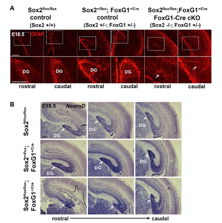
Evidence that Sox2+/-;FoxG1+/- hippocampi at E18.5 do not significantly differ from wild type (Sox2+/+, FoxG1+/+) controls. In contrast, Sox2-/-;FoxG1+/- hippocampi are severely defective. (A) GFAP immunofluorescence at E18.5 on coronal sections of control and FoxG1-Cre cKO hippocampi (controls n=6, mutants n=4). (B) In situ hybridization at E18.5 for NeuroD (controls n=4, mutants n=3) on coronal sections of control and FoxG1-Cre cKO hippocampi. Arrows indicate dentate gyrus (DG); note the strong decrease of the dentate gyrus, and the radial glia (GFAP) disorganization in cKO.<br /> The Sox2flox/flox genotype corresponds to wild type mice (Sox2+/+). The Sox2+/flox ; FoxG1Cre genotype corresponds to Sox2+/-; FoxG1+/- controls. The Sox2flox/flox ; FoxG1Cre genotype corresponds to Sox2-/-; FoxG1+/- mutants.
Reviewer #1:
Hutchings et al. report an updated cryo-electron tomography study of the yeast COP-II coat assembled around model membranes. The improved overall resolution and additional compositional states enabled the authors to identify new domains and interfaces--including what the authors hypothesize is a previously overlooked structural role for the SEC31 C-Terminal Domain (CTD). By perturbing a subset of these new features with mutants, the authors uncover some functional consequences pertaining to the flexibility or stability of COP-II assemblies.
Overall, the structural and functional work appears reliable, but certain questions and comments should be addressed prior to publication. However, this reviewer failed to appreciate the conceptual advance that warrants publication in a general biology journal like eLIFE. Rather, this study provides a valuable refinement of our understanding of COP-II that I believe is better suited to a more specialized, structure-focused journal.
We agree that in our original submission our description of the experimental setup, indeed similar to previous work, did not fully capture the novel findings of this paper. Rather than being simply a higher resolution structure of the COPII coat, in fact we have discovered new interactions in the COPII assembly network, and we have probed their functional roles, significantly changing our understanding of the mechanisms of COPII-mediated membrane curvature. In the revised submission we have included additional genetic data that further illuminate this mechanism, and have rewritten the text to better communicate the novel aspects of our work.
Our combination of structural, functional and genetic analyses goes beyond refining our textbook understanding of the COPII coat as a simple ‘adaptor and cage’, but rather it provides a completely new picture of how dynamic regulation of assembly and disassembly of a complex network leads to membrane remodelling.
These new insights have important implications for how coat assembly provides structural force to bend a membrane but is still able to adapt to distinct morphologies. These questions are at the forefront of protein secretion, where there is debate about how different types of carriers might be generated that can accommodate cargoes of different size.
Major Comments: 1) The authors belabor what this reviewer thinks is an unimportant comparison between the yeast reconstruction of the outer coat vertex with prior work on the human outer coat vertex. Considering the modest resolution of both the yeast and human reconstructions, the transformative changes in cryo-EM camera technology since the publication of the human complex, and the differences in sample preparation (inclusion of the membrane, cylindrical versus spherical assemblies, presence of inner coat components), I did not find this comparison informative. The speculations about a changing interface over evolutionary time are unwarranted and would require a detailed comparison of co-evolutionary changes at this interface. The simpler explanation is that this is a flexible vertex, observed at low resolution in both studies, plus the samples are very different.
We do agree that our proposal that the vertex interface changes over evolutionary time is speculative and we have removed this discussion. We agree that a co-evolutionary analysis will be enlightening here, but is beyond the scope of the current work.
We respectfully disagree with the reviewer’s interpretation that the difference between the two vertices is due to low resolution. The interfaces are clearly different, and the resolutions of the reconstructions are sufficient to state this. The reviewer’s suggestion that the difference in vertex orientation might be simply attributable to differences in sample, such as inclusion of the membrane, cylindrical versus spherical morphology, or presence of inner coat components were ruled out in our original submission: we resolved yeast vertices on spherical vesicles (in addition to those on tubes) and on membrane-less cages. These analyses clearly showed that neither the presence of a membrane, nor the change in geometry (tubular vs. spherical) affect vertex interactions. These experiments are presented in Supplementary Fig 4 (Supplementary Fig. 3 in the original version). Similarly, we discount that differences might be due to the presence or absence of inner coat components, since membrane-less cages were previously solved in both conditions and are no different in terms of their vertex structure (Stagg et al. Nature 2006 and Cell 2008).
We believe it is important to report on the differences between the two vertex structures. Nevertheless, we have shifted our emphasis on the functional aspects of vertex formation and moved the comparison between the two vertices to the supplement.
2) As one of the major take home messages of the paper, the presentation and discussion of the modeling and assignment of the SEC31-CTD could be clarified. First, it isn't clear from the figures or the movies if the connectivity makes sense. Where is the C-terminal end of the alpha-solenoid compared to this new domain? Can the authors plausibly account for the connectivity in terms of primary sequence? Please also include a side-by-side comparison of the SRA1 structure and the CTD homology model, along with some explanation of the quality of the model as measured by Modeller. Finally, even if the new density is the CTD, it isn't clear from the structure how this sub-stoichiometric and apparently flexible interaction enhances stability. Hence, when the authors wrote "when the [CTD] truncated form was the sole copy of Sec31 in yeast, cells were not viable, indicating that the novel interaction we detect is essential for COPII coat function." Maybe, but could this statement be a leap to far? Is it the putative interaction essential, or is the CTD itself essential for reasons that remain to be fully determined?
The CTD is separated from the C-terminus of the alpha solenoid domain by an extended domain (~350 amino acids) that is predicted to be disordered, and contains the PPP motifs and catalytic fragment that contact the inner coat. This is depicted in cartoon form in Figures 3A and 7, and discussed at length in the text. This arrangement explains why no connectivity is seen, or expected. We could highlight the C-terminus of the alpha-solenoid domain to emphasize where the disordered region should emerge from the rod, but connectivity of the disordered domain to the CTD could arise from multiple positions, including from an adjacent rod.
The reviewer’s point about the essentiality of the CTD being independent of its interaction with the Sec31 rod, is an important one. The basis for our model that the CTD enhances stability or rigidity of the coat is the yeast phenotype of Sec31-deltaCTD, which resembles that of a sec13 null. Both mutants are lethal, but rescued by deletion of emp24, which leads to more easily deformable membranes (Čopič et al. Science 2012). We agree that even if this model is true, the interaction of the CTD with Sec31 that our new structure reveals is not proven to drive rigidity or essentiality. We have tempered this hypothesis and added alternative possibilities to the discussion.
We have included the SRA1 structure in Supplementary Fig 5, as requested, and the model z-score in the Methods. The Z-score, as calculated by the proSA-web server is -6.07 (see figure below, black dot), and falls in line with experimentally determined structures including that of the template (PDB 2mgx, z-score = -5.38).
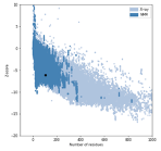
3) Are extra rods discussed in Fig. 4 are a curiosity of unclear functional significance? This reviewer is concerned that these extra rods could be an in vitro stoichiometry problem, rather than a functional property of COP-II.
This is an important point, that, as we state in the paper, cannot be answered at the moment: the resolution is too low to identify the residues involved in the interaction. Therefore we are hampered in our ability to assess the physiological importance of this interaction. We still believe the ‘extra’ rods are an important observation, as they clearly show that another mode of outer coat interaction, different from what was reported before, is possible.
The concern that interactions visualised in vitro might not be physiologically relevant is broadly applicable to structural biology approaches. However, our experimental approach uses samples that result from active membrane remodelling under near-physiological conditions, and we therefore expect these to be less prone to artefacts than most in vitro reconstitution approaches, where proteins are used at high concentrations and in high salt buffer conditions.
4) The clashsccore for the PDB is quite high--and I am dubious about the reliability of refining sidechain positions with maps at this resolution. In addition to the Ramchandran stats, I would like to see the Ramachandran plot as well as, for any residue-level claims, the density surrounding the modeled side chain (e.g. S742).
The clashscore is 13.2, which, according to molprobity, is in the 57th percentile for all structures and in the 97th for structures of similar resolutions. We would argue therefore that the clashscore is rather low. In fact, the model was refined from crystal structures previously obtained by other groups, which had worse clashscore (17), despite being at higher resolution. Our refinement has therefore improved the clashscore. During refinement we have chosen restraint levels appropriate to the resolution of our map (Afonine et al., Acta Cryst D 2018)
The Ramachandran plot is copied here and could be included in a supplemental figure if required. We make only one residue-level claim (S742), the density for which is indeed not visible at our resolution. We claim that S742 is close to the Sec23-23 interface, and do not propose any specific interactions. Nevertheless we have removed reference to S742 from the manuscript. We included this specific information because of the potential importance of this residue as a site of phosphorylation, thereby putting this interface in broader context for the general eLife reader.
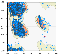
Minor Comments:
1) The authors wrote "To assess the relative positioning of the two coat layers, we analysed the localisation of inner coat subunits with respect to each outer coat vertex: for each aligned vertex particle, we superimposed the positions of all inner coat particles at close range, obtaining the average distribution of neighbouring inner coat subunits. From this 'neighbour plot' we did not detect any pattern, indicating random relative positions. This is consistent with a flexible linkage between the two layers that allows adaptation of the two lattices to different curvatures (Supplementary Fig 1E)." I do not understand this claim, since the pattern both looks far from random and the interactions depend on molecular interactions that are not random. Please clarify.
We apologize for the confusion: the pattern of each of the two coats are not random. Our sentence refers to the positions of inner and outer coats relative to each other. The two lattices have different parameters and the two layers are linked by flexible linkers (the 350 amino acids referred to above). We have now clarified the sentence.
2) Related to major point #1, the author wrote "We manually picked vertices and performed carefully controlled alignments." I do now know what it means to carefully control alignments, and fear this suggests human model bias.
We used different starting references for the alignments, with the precise aim to avoid model bias. For both vesicle and cage vertex datasets, we have aligned the subtomograms against either the vertex obtained from tubules, or the vertex from previously published membrane-less cages. In all cases, we retrieved a structure that resembles the one on tubules, suggesting that the vertex arrangement we observe isn’t simply the result of reference bias. This procedure is depicted in Supplementary Fig 4 (Supplementary Fig. 3 in the original manuscript), but we have now clarified it also in the methods section.
3) Why do some experiments use EDTA? I may be confused, but I was surprised to see the budding reaction employed 1mM GMPPNP, and 2.5mM EDTA (but no Magnesium?). Also, for the budding reaction, please replace or expand upon the "the 10% GUV (v/v)" with a mass or molar lipid-to-protein ratio.
We regret the confusion. As stated in the methods, all our budding reactions are performed in the presence of EDTA and Magnesium, which is present in the buffer (at 1.2 mM). The reason is to facilitate nucleotide exchange, as reported and validated in Bacia et al., Scientific Reports 2011.
Lipids in GUV preparations are difficult to quantify. We report the stock concentrations used, but in each preparation the amount of dry lipid that forms GUVs might be different, as is the concentration of GUVs after hydration. However since we analyse reactions where COPII proteins have bound and remodelled individual GUVs, we do not believe the protein/lipid ratio influences our structures.
4) Please cite the AnchorMap procedure.
We cite the SerialEM software, and are not aware of other citations specifically for the anchor map procedure.
5) Please edit for typos (focussing, functionl, others)
Done
Reviewer #2:
The manuscript describes new cryo-EM, biochemistry, and genetic data on the structure and function of the COPII coat. Several new discoveries are reported including the discovery of an extra density near the dimerization region of Sec13/31, and "extra rods" of Sec13/31 that also bind near the dimerization region. Additionally, they showed new interactions between the Sec31 C-terminal unstructured region and Sec23 that appear to bridge multiple Sec23 molecules. Finally, they increased the resolution of the Sec23/24 region of their structure compared to their previous studies and were able to resolve a previously unresolved L-loop in Sec23 that makes contact with Sar1. Most of their structural observations were nicely backed up with biochemical and genetic experiments which give confidence in their structural observations. Overall the paper is well-written and the conclusions justified.
However, this is the third iteration of structure determination of the COPII coat on membrane with essentially the same preparation and methods. Each time, there has been an incremental increase in resolution and new discoveries, but the impact of the present study is deemed to be modest. The science is good, but it may be more appropriate for a more specialized journal. Areas of specific concern are described below.
As described above, we respectfully disagree with this interpretation of the advance made by the current work. This work improves on previous work in many aspects. The resolution of the outer coat increases from over 40A to 10-12A, allowing visualisation of features that were not previously resolved, including a novel vertex arrangement, the Sec31 CTD, and the outer coat ‘extra rods’. An improved map of the inner coat also allows us to resolve the Sec23 ‘L-loop’. We would argue that these are not just extra details, but correspond to a suite of novel interactions that expand our understanding of the complex COPII assembly network. Moreover, we include biochemical and genetic experiments that not only back up our structural observations but bring new insights into COPII function. As pointed out in response to reviewer 1, we believe our work contributes a significant conceptual advance, and have modified the manuscript to convey this more effectively.
1) The abstract is vague and should be re-written with a better description of the work.
We have modified the abstract to specifically outline what we have done and the major new discoveries of this paper.
2) Line 166 - "Surprisingly, this mutant was capable of tubulating GUVs". This experiment gets to one of the fundamental unknown questions in COPII vesiculation. It is not clear what components are driving the membrane remodeling and at what stages during vesicle formation. Isn't it possible that the tubulation activity the authors observe in vitro is not being driven at all by Sec13/31 but rather Sec23/24-Sar1? Their Sec31ΔCTD data supports this idea because it lacks a clear ordered outer coat despite making tubules. An interesting experiment would be to see if tubules form in the absence of all of Sec13/31 except the disordered domain of Sec31 that the authors suggest crosslinks adjacent Sec23/24s.
This is an astute observation, and we agree with the reviewer that the source of membrane deformation is not fully understood. We favour the model that budding is driven significantly by the Sec23-24 array. To further support this, we have performed a new experiment, where we expressed Sec31ΔN in yeast cells lacking Emp24, which have more deformable membranes and are tolerant to the otherwise lethal deletion of Sec13. While Sec31ΔN in a wild type background did not support cell viability, this was rescued in a Δemp24 yeast strain, strongly supporting the hypothesis that a major contributor to membrane remodelling is the inner coat, with the outer coat becoming necessary to overcome membrane bending resistance that ensues from the presence of cargo. We now include these results in Figure 1.
However, we must also take into account the results presented in Fig. 6, where we show that weakening the Sec23-24 interface still leads to budding, but only if Sec13-31 is fully functional, and that in this case budding leads to connected pseudo-spherical vesicles rather than tubes. When Sec13-31 assembly is also impaired, tubes appear unstructured. We believe this strongly supports our conclusions that both inner and outer coat interactions are fundamental for membrane remodelling, and it is the interplay between the two that determines membrane morphology (i.e. tubes vs. spheres).
To dissect the roles of inner and outer coats even further, we have done the experiment that the reviewer suggests: we expressed Sec31768-1114, but the protein was not well-behaved and co-purified with chaperones. We believe the disordered domain aggregates when not scaffolded by the structured elements of the rod. Nonetheless, we used this fragment in a budding reaction, and could not see any budding. We did not include this experiment as it was inconclusive: the lack of functionality of the purified Sec31 fragment could be attributed to the inability of the disordered region to bind its inner coat partner in the absence of the scaffolding Sec13-31 rod. As an alternative approach, we have used a version of Sec31 that lacks the CTD, and harbours a His tag at the N-terminus (known from previous studies to partially disrupt vertex assembly). We think this construct is more likely to be near native, since both modifications on their own lead to functional protein. We could detect no tubulation with this construct by negative stain, while both control constructs (Sec31ΔCTD and Nhis-Sec31) gave tubulation. This suggests that the cross-linking function of Sec31 is not sufficient to tubulate GUV membranes, but some degree of functional outer coat organisation (either mediated by N- or C-terminal interactions) is needed. It is also possible that the lack of outer coat organisation might lead to less efficient recruitment to the inner coat and cross-linking activity. We have added this new observation to the manuscript.
3) Line 191 - "Inspecting cryo-tomograms of these tubules revealed no lozenge pattern for the outer 192 coat" - this phrasing is vague. The reviewer thinks that what they mean is that there is a lack of order for the Sec13/31 layer. Please clarify.
The reviewer is correct, we have changed the sentence.
4) Line 198 - "unambiguously confirming this density corresponds to 199 the CTD." This only confirms that it is the CTD if that were the only change and the Sec13/31 lattice still formed. Another possibility is that it is density from other Sec13/31 that only appears when the lattice is formed such as the "extra rods". One possibility is that the density is from the extra rods. The reviewer agrees that their interpretation is indeed the most likely, but it is not unambiguous. The authors should consider cross-linking mass spectrometry.
We have removed the word ‘unambiguously’, and changed to ‘confirming that this density most likely corresponds to the CTD’. Nonetheless, we believe that our interpretation is correct: the extra rods bind to a different position, and themselves also show the CTD appendage. In this experiment, the lack of the CTD was the only biochemical change.
5) In the Sec31ΔCTD section, the authors should comment on why ΔCTD is so deleterious to oligomer organization in yeast when cages form so abundantly in preparations of human Sec13/31 ΔC (Paraan et al 2018).
We have added a comment to address this. “Interestingly, human Sec31 proteins lacking the CTD assemble in cages, indicating that either the vertex is more stable for human proteins and sufficient for assembly, or that the CTD is important in the context of membrane budding but not for cage formation in high salt conditions.”
6) The data is good for the existence of the "extra rods", but significance and importance of them is not clear. How can these extra densities be distinguished from packing artifacts due to imperfections in the helical symmetry.
Please also see our response to point 3 from reviewer 1. Regarding the specific concern that artefacts might be a consequence of imperfection in the helical symmetry, we would argue such imperfections are indeed expected in physiological conditions, and to a much higher extent. For this reason interactions seen in the context of helical imperfections are likely to be relevant. In fact, in normal GTP hydrolysis conditions, we expect long tubes would not be able to form, and the outer coat to be present on a wide range of continuously changing membrane curvatures. We think that the ability of the coat to form many interactions when the symmetry is imperfect might be exactly what confers the coat its flexibility and adaptability.
7) Figure 5 is very hard to interpret and should be redone. Panels B and C are particularly hard to interpret.
We have made a new figure where we think clarity is improved.
8) The features present in Sec23/24 structure do not reflect the reported resolution of 4.7 Å. It seems that the resolution is overestimated.
We report an average resolution of 4.6 Å. In most of our map we can clearly distinguish beta strands, follow the twist of alpha helices and see bulky side chains. These features typically become visible at 4.5-5A resolution. We agree that some areas are worse than 4.6 Å, as typically expected for such a flexible assembly, but we believe that the average resolution value reported is accurate. We obtained the same resolution estimate using different software including relion, phenix and dynamo, so that is really the best value we can provide. To further convince ourselves that we have the resolution we claim, we sampled EM maps from the EMDB with the same stated resolution (we just took the 7 most recent ones which had an associated atomic model), and visualised their features at arbitrary positions. For both beta strands and alpha helices, we do not feel our map looks any worse than the others we have examined. We include a figure here.
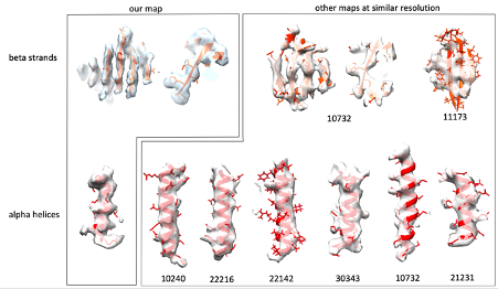
9) Lines 315/316 - "We have combined cryo-tomography with biochemical and genetic assays to obtain a complete picture of the assembled COPII coat at unprecedented resolution (Fig. 7)"
10) Figure 7. is a schematic model/picture the authors should reference a different figure or rephrase the sentence.
We now refer to Fig 7 in a more appropriate place.
Reviewer #3:
The manuscript by Hutchings et al. describes several previously uncharacterised molecular interactions in the coats of COP-II vesicles by using a reconstituted coats of yeast COPI-II. They have improved the resolution of the inner coat to 4.7A by tomography and subtomogram averaging, revealing detailed interactions, including those made by the so-called L-loop not observed before. Analysis of the outer layer also led to new interesting discoveries. The sec 31 CTD was assigned in the map by comparing the WT and deletion mutant STA-generated density maps. It seems to stabilise the COP-II coats and further evidence from yeast deletion mutants and microsome budding reconstitution experiments suggests that this stabilisation is required in vitro. Furthermore, COP-II rods that cover the membrane tubules in right-handed manner revealed sometimes an extra rod, which is not part of the canonical lattice, bound to them. The binding mode of these extra rods (which I refer to here a Y-shape) is different from the canonical two-fold symmetric vertex (X-shape). When the same binding mode is utilized on both sides of the extra rod (Y-Y) the rod seems to simply insert in the canonical lattice. However, when the Y-binding mode is utilized on one side of the rod and the X-binding mode on the other side, this leads to bridging different lattices together. This potentially contributes to increased flexibility in the outer coat, which maybe be required to adopt different membrane curvatures and shapes with different cargos. These observations build a picture where stabilising elements in both COP-II layers contribute to functional cargo transport. The paper makes significant novel findings that are described well. Technically the paper is excellent and the figures nicely support the text. I have only minor suggestions that I think would improve the text and figure.
We thank the reviewer for helpful suggestions which we agree improve the manuscript.
Minor Comments:
L 108: "We collected .... tomograms". While the meaning is clear to a specialist, this may sound somewhat odd to a generic reader. Perhaps you could say "We acquired cryo-EM data of COP-II induced tubules as tilt series that were subsequently used to reconstruct 3D tomograms of the tubules."
We have changed this as suggested
L 114: "we developed an unbiased, localisation-based approach". What is the part that was developed here? It seems that the inner layer particle coordinates where simply shifted to get starting points in the outer layer. Developing an approach sounds more substantial than this. Also, it's unclear what is unbiased about this approach. The whole point is that it's biased to certain regions (which is a good thing as it incorporates prior knowledge on the location of the structures).
We have modified the sentence to “To target the sparser outer coat lattice for STA, we used the refined coordinates of the inner coat to locate the outer coat tetrameric vertices”, and explain the approach in detail in the methods.
L 124: "The outer coat vertex was refined to a resolution of approximately ~12 A, revealing unprecedented detail of the molecular interactions between Sec31 molecules (Supplementary Fig 2A)". The map alone does not reveal molecular interactions; the main understanding comes from fitting of X-ray structures to the low-resolution map. Also "unprecedented detail" itself is somewhat problematic as the map of Noble et al (2013) of the Sec31 vertex is also at nominal resolution of 12 A. Furthermore, Supplementary Fig 2A does not reveal this "unprecedented detail", it shows the resolution estimation by FSC. To clarify, these points you could say: "Fitting of the Sec31 atomic model to our reconstruction vertex at 12-A resolution (Supplementary Fig 2A) revealed the molecular interactions between different copies of Sec31 in the membrane-assembled coat.
We have changed the sentence as suggested.
L 150: Can the authors exclude the possibility that the difference is due to differences in data processing? E.g. how the maps amplitudes have been adjusted?
Yes, we can exclude this scenario by measuring distances between vertices in the right and left handed direction. These measurements are only compatible with our vertex arrangement, and cannot be explained by the big deviation from 4-fold symmetry seen in the membrane-less cage vertices.
L 172: "that wrap tubules either in a left- or right-handed manner". Don't they do always both on each tubule? Now this sentence could be interpreted to mean that some tubules have a left-handed coat and some a right-handed coat.
We have changed this sentence to clarify. “Outer coat vertices are connected by Sec13-31 rods that wrap tubules both in a left- and right-handed manner.”
L276: "The difference map" hasn't been introduced earlier but is referred to here as if it has been.
We now introduce the difference map.
L299: Can "Secondary structure predictions" denote a protein region "highly prone to protein binding"?
Yes, this is done through DISOPRED3, a feature include in the PSIPRED server we used for our predictions. The reference is: Jones D.T., Cozzetto D. DISOPRED3: precise disordered region predictions with annotated protein-binding activity Bioinformatics. 2015; 31:857–863. We have now added this reference to the manuscript.
L316: It's true that the detail in the map of the inner coat is unprecedented and the model presented in Figure 7 is partially based on that. But here "unprecedented resolution" sounds strange as this sentence refers to a schematic model and not a map.
We have changed this by moving the reference to Fig 7 to a more appropriate place
L325: "have 'compacted' during evolution" -> remove. It's enough to say it's more compact in humans and less compact in yeast as there could have been different adaptations in different organisms at this interface.
We have changed as requested. See also our response to reviewer 1, point 1.
L327: What's exactly meant by "sequence diversity or variability at this density".
We have now clarified: “Since multiple charge clusters in yeast Sec31 may contribute to this interaction interface (Stancheva et al., 2020), the low resolution could be explained by the fact that the density is an average of different sequences.”
L606-607: The description of this custom data processing approach is difficult to follow. Why is in-plane flip needed and how is it used here?
Initially particles are picked ignoring tube directionality (as this cannot be assessed easily from the tomograms due to the pseudo-twofold symmetry of the Sec23/24/Sar1 trimer). So the in plane rotation of inner coat subunit could be near 0 or 180°. For each tube, both angles are sampled (in-plane flip). Most tubes result in the majority of particles being assigned one of the two orientations (which is then assumed as the tube directionality). Particles that do not conform are removed, and rare tubes where directionality cannot be determined are also removed. We have re-written the description to clarify these points: “Initial alignments were conducted on a tube-by-tube basis using the Dynamo in-plane flip setting to search in-plane rotation angles 180° apart. This allowed to assign directionality to each tube, and particles that were not conforming to it were discarded by using the Dynamo dtgrep_direction command in custom MATLAB scripts”
L627: "Z" here refers to the coordinate system of aligned particles not that of the original tomogram. Perhaps just say "shifted 8 pixels further away from the membrane".
Changed as requested.
L642-643: How can the "left-handed" and "right-handed" rods be separated here? These terms refer to the long-range organisation of the rods in the lattice it's not clear how they were separated in the early alignments.
They are separated by picking only one subset using the dynamo sub-boxing feature. This extracts boxes from the tomogram which are in set positions and orientation relative to the average of previously aligned subtomograms. From the average vertex structure, we sub-box rods at 4 different positions that correspond to the centre of the rods, and the 2-fold symmetric pairs are combined into the same dataset. We have clarified this in the text: “The refined positions of vertices were used to extract two distinct datasets of left and right-handed rods respectively using the dynamo sub-boxing feature.”
Figure 2B. It's difficult to see the difference between dark and light pink colours.
We have changed colours to enhance the difference.
Figure 3C. These panels report the relative frequency of neighbouring vertices at each position; "intensity" does not seem to be the right measure for this. You could say that the colour bar indicates the "relative frequency of neighbouring vertices at each position" and add detail how the values were scaled between 0 and 1. The same applies to SFigure 1E.
Changed as requested.
Figure 4. The COP-II rods themselves are relatively straight, and they are not left-handed or right-handed. Here, more accurate would be "architecture of COPII rods organised in a left-handed manner". (In the text the authors may of course define and then use this shorter expression if they so wish.) Panel 4B top panel could have the title "left-handed" and the lower panel should have the title "right-handed" (for consistency and clarity).
We have now defined left- and right-handed rods in the text, and have changed the figure and panel titles as requested.
We thank the reviewers for their comments, which will improve the quality of our manuscript.
Our study describes a novel approach to the identification of GTPase binding-partners. We recapitulated and augmented previous protein-protein interaction data for RAB18 and presented data validating some of our findings. In aggregate, our dataset suggested that RAB18 modulates the establishment of membrane contact sites and the transfer of lipid between closely apposed membranes.
In the original version of our manuscript, we stated that we were exploring the possibility that RAB18 contributes to cholesterol biosynthesis by mobilizing substrates or products of the Δ8-Δ7 sterol isomerase emopamil binding protein (EBP). While our manuscript was under review, we profiled sterols in wild-type and RAB18-null cells and assayed cholesterol biosynthesis in a panel of cell lines (Figure 1).
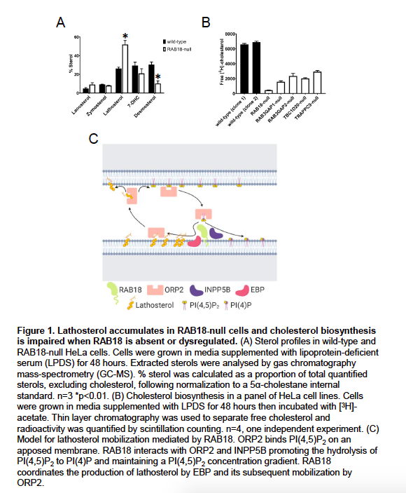
Our new data show that an EBP-product, lathosterol, accumulates in RAB18-null cells (p<0.01). Levels of a downstream cholesterol intermediate, desmosterol, are reduced in these cells (p<0.01) consistent with impaired delivery of substrates to post-EBP biosynthetic enzymes (Figure 1A). Further, our preliminary data suggests that cholesterol biosynthesis is substantially reduced when RAB18 is absent or dysregulated (4 technical replicates, one independent experiment) (Figure 1B).
Because of the clinical overlap between Micro syndrome and cholesterol biosynthesis disorders including Smith-Lemli-Opitz syndrome (SLOS; MIM 270400) and lathosterolosis (MIM 607330), our new findings suggest that impaired cholesterol biosynthesis may partly underlie Warburg Micro syndrome pathology. Therapeutic strategies have been developed for the treatment of SLOS and lathosterolosis, and so confirmation of our findings may spur development of similar strategies for Micro syndrome.
Our new findings provide further functional validation of our methodology and support our interpretation of our protein interaction data.
Reply to point 1)
Tetracycline-induced expression of wild-type and mutant BirA*-RAB18 fusion proteins in the stable HEK293 cell lines was quantified by densitometry (Figure 2).
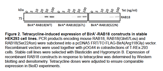
For the HEK293 BioID experiments, tetracycline dosage was adjusted to ensure comparable expression levels. We will include these data in supplemental material in an updated version of our manuscript.
The localization of wild-type and mutant forms of RAB18 in HEK293 cells is somewhat different consistent with previous reports (Ozeki et al. 2005)(Figure 3).
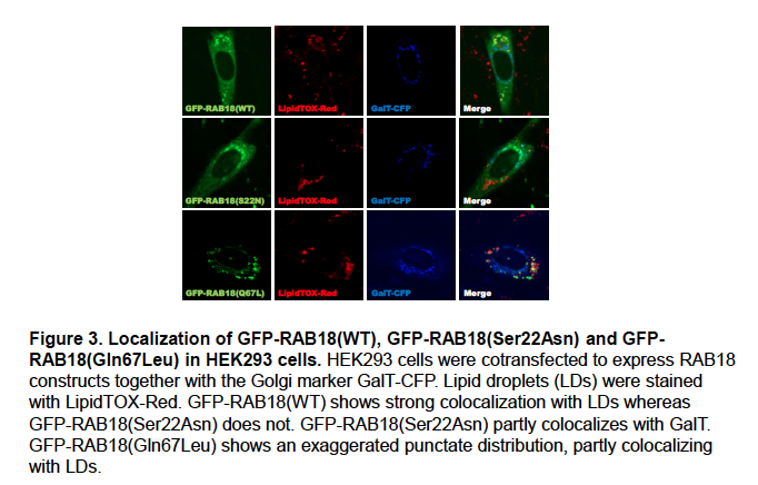
We feel that this may reflect the differential localization of ‘active’ and ‘inactive’ RAB18, with wild-type RAB18 corresponding to a mixture of the two. We will include these data in supplemental material in an updated version of our manuscript.
We acknowledge that the differential localization of wild-type and mutant BirA*-RAB18 might influence the compliment of proteins labeled by these constructs. Nevertheless, we feel that the RAB18(S22N):RAB18(WT) ratios are useful since they distinguish a number of previously-identified RAB18-interactors (manuscript, Figure 1B).
Reply to point 2)
For the HEK293 dataset, spectral counts are provided and for the HeLa dataset LFQ intensities were provided in the manuscript (manuscript, Tables S1 and S2 respectively). However, we did not find that these were useful classifiers for ranking functional interactions when used in isolation.
The extent of labelling produced in a BioID experiment is not wholly determined by the kinetics of protein-protein associations. It is also influenced by, for example, protein abundance, the number and location of exposed surface lysine residues, and protein stability over the timcourse of labelling. We feel that RAB18(S22N):RAB18(WT) and GEF-null:wild-type ratios were helpful in controlling for these factors. Further, that our comparative approach was effective in highlighting known RAB18-interactors and in identifying novel ones.
We acknowledge that our approach may omit some bona fide functional RAB18-interactions, but would argue that our aims were to augment existing functional RAB18-interaction data and avoid false-positives, rather than to emphasise completeness.
Reply to point 3)
We will include representative fluorescence images for the SEC22A, NBAS and ZW10 knockdown experiments in an updated version of our manuscript.
Unfortunately, a suitable antibody for determining knockdown efficiency of SEC22A at the protein level is not commercially available. We will determine SEC22A knockdown efficiency at the mRNA level using qPCR.
Reply to point 4)
Expression levels of wild-type and mutant RAB18 in the stable CHO cell lines generated for this study were determined by Western blotting and found to be comparable (Figure 4).
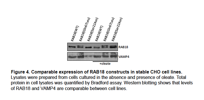
We will include these data in supplemental material in an updated version of our manuscript.
The levels of [14C]-CE were higher in RAB18(Gln67Leu) cells than in the other cell lines following loading with [14C]-oleate for 24 hours. We will amend the text to make this explicit. Our interpretation of the data is that ‘active’ RAB18 facilitates the mobilization of cholesterol. When cells are loaded with oleate, this promotes generation and storage of CE. Conversely, when cells are treated with HDL, it promotes more rapid efflux.
Our new data implicating RAB18 in the mobilization of lathosterol supports our interpretation of our loading and efflux experiments. In the light of our new data showing that de novo cholesterol biosynthesis is impaired when RAB18 is absent or dysregulated, it will be interesting to determine whether cholesterol synthesis is increased in the RAB18(Gln67Leu) cells.
Reply to point 1)
We anticipate that the approach of comparative proximity biotinylation in GEF-null and wild-type cell lines will be broadly useful in small GTPase research.
While RAB18 has previously been implicated in regulating membrane contacts, the identification of SEC22A as a RAB18-interactor adds to the previous model for their assembly.
While ORP2 and INPP5B have previously been shown to mediate cholesterol mobilization, the novel finding that they both interact with RAB18 adds to this work. We argue that RAB18-ORP2-INPP5B functions in an analogous manner to ARF1-OSBP-SAC1 in mediating sterol exchange. The broad Rab-binding specificity of multiple OSBP-homologs, and that of multiple phosphoinositide phosphatase enzymes, suggests that this may be a common conserved relationship.
Our new data indicating that RAB18 coordinates generation of sterol intermediates by EBP and their delivery to post-EBP biosynthetic enzymes reveals a new role for Rab proteins in lipid biogenesis. Most importantly, our new findings that RAB18 deficiency is associated with impaired cholesterol biogenesis suggest that Warburg Micro syndrome is a cholesterol biogenesis disorder. Further, that it may be amenable to therapeutic intervention.
Reply to point 2)
Recognising that the effect of RAB18 on cholesterol esterification and efflux could arise from various causes, we previously carried out Western blotting of the CHO cell lines for ABCA1 to determine whether this protein was involved (Figure 5).
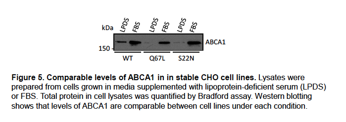
Similar levels of ABCA1 expression in these lines suggests it is not. We will include these data in supplemental material in an updated version of our manuscript.
We feel that our new data implicating RAB18 in lathosterol mobilization provides important insight into its role in cholesterol biogenesis. Further, it supports our previous suggestion that RAB18 mediates cholesterol mobilization.
Reply to point 3)
We agree that the established roles for ORP2, TMEM24/C2CD2L and PIP2 at the plasma membrane make this an extremely interesting area for future research; it is one we are actively investigating. However, we respectfully feel that to comprehensively explore the subcellular locations of RAB18-mediated sterol/PIP2 exchange requires another study and is beyond the scope of the present report.
Reply to point 1)
The RAB18-SPG20 interaction has already been validated with a co-immunoprecipitation experiment (Gillingham et al. 2014). We will update the text of our manuscript to make this more explicit, but do not feel it is necessary to recapitulate this work.
We argue in the manuscript that RAB18 may coordinate the assembly of a non-canonical SNARE complex incorporating SEC22A, STX18, BNIP1 and USE1. However, this role may be mediated through prior interaction with the NBAS-RINT1-ZW10 (NRZ) tethering complex and the SM-protein SCFD2 rather than through a direct interaction. We therefore feel that a RAB18-SEC22A interaction may be difficult to validate by conventional means.
The reciprocal experiments with BioID2(Gly40S)-SEC22A did provide tentative confirmation of the interaction together with evidence that a subset of SEC22A-interactions are attenuated when RAB18 is absent or dysregulated. In the light of our new findings reinforcing a role for RAB18 in sterol mobilization at membrane contact sites, it is interesting that one of these is DHRS7, an enzyme with steroids among its putative substrates.
Reply to point 2)
We previously analysed the localization of the BirA*-RAB18 fusion protein in HeLa cells (Figure 6).
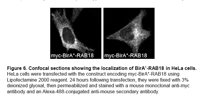
It shows a reticular staining pattern consistent with the reported localization of RAB18 to the ER (Gerondopoulos et al. 2014; Ozeki et al. 2005). We will include these data in supplemental material in an updated version of our manuscript.
Heterologous expression of the BirA*-RAB18 fusion protein in HeLa cells identified the interactions between RAB18 and EBP, ORP2 and INPP5B, for which we now have supportive functional evidence. Since the evidence for impaired lathosterol mobilization and cholesterol biosynthesis was derived from experiments on null-cells, in which endogenous protein expression is absent, we feel that rescue experiments are not necessary in the present study. However, such experiments could be highly useful in future studies.
Reply to point 3)
Our screening approach did use both a RAB3GAP-null:wild-type comparison (manuscript, Figure 2, Table S2) and also a RAB18(S22N):RAB18(WT) comparison (manuscript, Figure 1, Table S1). Differences should be expected between these datasets, since they used different cell lines and slightly different methodologies. Nevertheless, proteins identified in both datasets included the known RAB18 effectors NBAS, RINT1, ZW10 and SCFD2, and the novel potential effectors CAMSAP1 and FAM134B.
There is prior evidence for 12 of the 25 RAB3GAP-dependent RAB18 interactions we identified (manuscript, Figure 2D). Among the 6 lipid modifying/mobilizing proteins found exclusively in our HeLa dataset, we previously presented direct evidence for the interaction of RAB18 with TMCO4. We now also have strong functional evidence for its interaction with EBP, ORP2 and INPP5B.
Reply to point 4)
It has been reported that knockdown of SEC22B does not affect the size distribution of lipid droplets (Xu et al. 2018) Figure 8H). Nevertheless, we will carry out qPCR experiments to determine whether the SEC22A siRNAs used in our study affect SEC22B expression. We have found that exogenous expression of SEC22A can cause cellular toxicity. Rescue experiments would therefore be difficult to perform.
Reply to point 5)
The background fluorescence measured in SPG20-null cells and presented in Figure 4B in the manuscript does not imply that the SPG20 antibody shows significant cross-reactivity. Rather, it reflects the fact that fluorescence intensity is recorded by our Operetta microscope in arbitrary units.
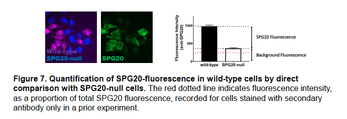
Above (Figure 7), is a version of the panel in which fluorescence from staining cells with only the secondary antibody is included (recorded in a previous experiment and expressed as a proportion of total SPG20 fluorescence in this experiment).
We have found that comparative fluorescence microscopy is more sensitive than immunoblotting. The SPG20 antibody we used to stain the HeLa cells has previously been used in quantitative fluorescence microscopy (Nicholson et al. 2015).
Furthermore, we showed corresponding, significantly reduced, expression of SPG20 in RAB18- and TBC1D20-null RPE1 cells, using quantitative proteomics (manuscript, Table S3).
We acknowledge that quantification of SPG20 transcript levels would clarify the level at which it is downregulated and will carry out qPCR experiments accordingly.
Reply to point 6)
We interpret both the enhanced CE-synthesis following oleate-loading and the rapid efflux upon incubation with HDL (manuscript, Figure 7A) as resulting from increased cholesterol mobilization. Our new data implicating RAB18 in the mobilization of lathosterol support this interpretation.
In the [3H]-cholesterol efflux assay (manuscript, Figure 7B) total [3H]-cholesterol loading at t=0 was 156392±8271 for RAB18(WT) cells, 168425±9103 for RAB18(Gln67Leu) cells and 148867±7609 (cpm determined through scintillation counting). Normalizing to total cellular radioactivity assured that differences in loading between replicates did not skew the results.
The candidate effector likely to directly mediate cholesterol mobilization is ORP2. It has been shown that ORP2 overexpression drives cholesterol to the plasma membrane (Wang et al. 2019). Further, there is evidence for reduced plasma membrane cholesterol in ORP2-null cells (Wang et al. 2019).
We previously carried out Western blotting of the CHO cell lines for ABCA1 to determine whether this protein was involved in altered efflux (Figure 5, above). Similar levels of ABCA1 expression in these lines suggests it is not. We will include these data in supplemental material in an updated version of our manuscript.
References
Gerondopoulos, A., R. N. Bastos, S. Yoshimura, R. Anderson, S. Carpanini, I. Aligianis, M. T. Handley, and F. A. Barr. 2014. 'Rab18 and a Rab18 GEF complex are required for normal ER structure', J Cell Biol, 205: 707-20.
Gillingham, A. K., R. Sinka, I. L. Torres, K. S. Lilley, and S. Munro. 2014. 'Toward a comprehensive map of the effectors of rab GTPases', Dev Cell, 31: 358-73.
Nicholson, J. M., J. C. Macedo, A. J. Mattingly, D. Wangsa, J. Camps, V. Lima, A. M. Gomes, S. Doria, T. Ried, E. Logarinho, and D. Cimini. 2015. 'Chromosome mis-segregation and cytokinesis failure in trisomic human cells', eLife, 4.
Ozeki, S., J. Cheng, K. Tauchi-Sato, N. Hatano, H. Taniguchi, and T. Fujimoto. 2005. 'Rab18 localizes to lipid droplets and induces their close apposition to the endoplasmic reticulum-derived membrane', J Cell Sci, 118: 2601-11.
Wang, H., Q. Ma, Y. Qi, J. Dong, X. Du, J. Rae, J. Wang, W. F. Wu, A. J. Brown, R. G. Parton, J. W. Wu, and H. Yang. 2019. 'ORP2 Delivers Cholesterol to the Plasma Membrane in Exchange for Phosphatidylinositol 4, 5-Bisphosphate (PI(4,5)P2)', Mol Cell, 73: 458-73 e7.
Xu, D., Y. Li, L. Wu, Y. Li, D. Zhao, J. Yu, T. Huang, C. Ferguson, R. G. Parton, H. Yang, and P. Li. 2018. 'Rab18 promotes lipid droplet (LD) growth by tethering the ER to LDs through SNARE and NRZ interactions', J Cell Biol, 217: 975-95.
This paper addresses the very interesting topic of genome evolution in asexual animals. While the topic and questions are of interest, and I applaud the general goal of a large-scale comparative approach to the questions, there are limitations in the data analyzed. Most importantly, as the authors raise numerous times in the paper, questions about genome evolution following transitions to asexuality inherently require lineage-specific controls, i.e. paired sexual species to compare with the asexual lineages. Yet such data are currently lacking for most of the taxa examined, leaving a major gap in the ability to draw important conclusions here. I also do not think the main positive results, such as the role of hybridization and ploidy on the retention and amount of heterozygosity, are novel or surprising.
We agree with the reviewer that having the sexual outgroups would improve the interpretations; this is one of the points we make in our manuscript. Importantly however, all previous genome studies of asexual species focus on individual asexual lineages, generally without sexual species for comparison. Yet reported genome features have been interpreted as consequences of asexuality (e.g., Flot et al. 2013). By analysing and comparing these genomes, we can show that these features are in fact lineage-specific rather than general consequences of asexuality. Unexpectedly, we find that asexuals that are not of hybrid origin are largely homozygous, independently of the cellular mechanism underlying asexuality. This contrasts with the general view that cellular mechanisms such as central fusion (which facilitates heterozygosity retention between generation) promotes the evolutionary success of asexual lineages relative to mechanisms such as gamete duplication (which generate complete homozygosity) by delaying the expression of the recessive load. We also do not observe the expected relationship between cellular mechanism of asexuality and heterozygosity retention in species of hybrid origin. Thus we respectfully disagree that our results are not surprising. Reviewer #2 found our results “interesting” and a “potentially important contribution”, and reviewer #3 wrote that we “call into question the generality of the theoretical expectations, and suggest that the genomic impacts of asexuality may be more complicated than previously thought”.
We also make it very clear that some of the patterns we uncover (e.g. low TE loads in asexual species) cannot be clearly evaluated with asexuals alone. Our study emphasizes the importance of the fact that asexuality is a lineage-level trait and that comparative analyses using asexuals requires lineage-level replication in addition to comparisons to sexual species.
References
Flot, Jean-François, et al. "Genomic evidence for ameiotic evolution in the bdelloid rotifer Adineta vaga." Nature 500.7463 (2013): 453-457.
[...] Major Issues and Questions:
1) The authors choose to refer to asexuality when describing thelytokous parthenogenesis. Asexuality is a very general term that can be confusing: fission, vegetative reproduction could also be considered asexuality. I suggest using parthenogenesis throughout the manuscript for the different animal clades studied here. Moreover, in thelytokous parthenogenesis meiosis can still occur to form the gametes, it is therefore not correct to write that "gamete production via meiosis... no longer take place" (lines 57-58). Fertilization by sperm indeed does not seem to take place (except during hybridogenesis, a special form of parthenogenesis).
We will clarify more explicitly what asexuality refers to in our manuscript. Notably our study does not include species that produce gametes which are fertilized (which is the case under hybridogenesis, which sensu stricto is not a form of parthenogenesis). Even though many forms of parthenogenesis do indeed involve meiosis (something we explain in much detail in box 2), there is no production of gametes.
2) The cellular mechanisms of asexuality in many asexual lineages are known through only a few, old cytological studies and could be inaccurate or incomplete (for example Triantaphyllou paper of 1981 of Meloidogyne nematodes or Hsu, 1956 for bdelloid rotifers). The authors should therefore mention in the introduction the lack of detailed and accurate cellular and genetic studies to describe the mode of reproduction because it may change the final conclusion.
For example, for bdelloid rotifers the literature is scarce. However the authors refer in Supp Table 1 to two articles that did not contain any cytological data on oogenesis in bdelloid rotifers to indicate that A. vaga and A. ricciae use apomixis as reproductive mode. Welch and Meselson studied the karyotypes of bdelloid rotifers, including A. vaga, and did not conclude anything about absence or presence of chromosome homology and therefore nothing can be said about their reproduction mode. In the article of Welch and Meselson the nuclear DNA content of bdelloid species is measured but without any link with the reproduction mode. The only paper referring to apomixis in bdelloids is from Hsu (1956) but it is old and new cytological data with modern technology should be obtained.
We will correct the rotifer citations and thank the reviewer for picking up the error. We agree that there are uncertainties in some cytological studies, but the same is true for genomic studies (which is why we base our analyses as much as possible on raw reads rather than assemblies because the latter may be incorrect). We in fact excluded cytological studies where the findings could not be corroborated. For example, we discarded the evidence for meiosis and diploidy by Handoo at al. 2004 for its incompatibility with genomic data because this study does not provide any verifiable evidence (there are no data or images, only descriptions of observations). We provide all the references in the supplementary material concerning the cytological evidence used.
3) In the section on Heterozygosity, the authors compute heterozygosity from kmer spectra analysis from reads to "avoid biases from variable genome assembly qualities" (page 16). But such kmer analysis can be biased by the quality and coverage of sequencing reads. While such analyses are a legitimate tool for heterozygosity measurements, this argument (the bias of genome quality) is not convincing and the authors should describe the potential limits of using kmer spectra analyses.
We excluded all the samples with unsuitable quality of data (e.g. one tardigrade species with excessive contamination or the water flea samples for insufficient coverage), and T. Rhyker Ranallo Benavidez, the author of the method we used, collaborated with us on the heterozygosity analyzes. However, we will clarify the limitations of the method for species with extremely low or high heterozygosity (see also comment 5 of this reviewer).
4) The authors state that heterozygosity levels “should decay over time for most forms of meiotic asexuality". This is incorrect, as this is not expected with "central fusion" or with "central fusion automixis equivalent" where there is no cytokinesis at meiosis I.
Our statement is correct. Note that we say “most” and not “all” because certain forms of endoduplication in F1 hybrids result in the maintenance of heterozygosity. Central fusion is expected to fully retain heterozygosity only if recombination is completely suppressed (see for example Suomalainen et al. 1987 or Engelstädter 2017).
5) I do not fully agree with the authors’ statement that: "In spite of the prediction that the cellular mechanism of asexuality should affect heterozygosity, it appears to have no detectable effect on heterozygosity levels once we control for the effect of hybrid origins (Figure 2)." (page 17)
The scaling on Figure 2 is emphasizing high values, while low values are not clearly separated. By zooming in on the smaller heterozygosity % values we may observe a bigger difference between the "asexuality mechanisms". I do not see how asexuality mechanism was controlled for, and if you look closely at intra group heterozygosity, variability is sometimes high.
It is expected that hybrid origin leads to higher heterozygosity levels but saying that asexuality mechanism is not important is surprising: on Figure 2 the orange (central fusion) is always higher than yellow (gamete duplication).
As we explain in detail in the text, the three comparatively high heterozygosity values under spontaneous origins of asexuality (“orange” points in the bottom left corner of the figure) are found in an only 40-year old clone of the Cape bee. Among species of hybrid origin, we see no correlation between asexuality mechanism and heterozygosity. These observations suggest that the asexuality mechanism may have an impact on genome-wide heterozygosity in recent incipient asexual lineages, but not in established asexual lineages.
Also, the variability found within rotifers could be an argument against a strong importance of asexuality origin on heterozygosity levels: the four bdelloid species likely share the same origin but their allelic heterozygosity levels appears to range from almost 0 to almost 6% (Fig 2 and 3, however the heterozygosity data on Rotaria should be confirmed, see below).
We prefer not using the data from rotifers for making such arguments, given the large uncertainty with respect to genome features in this group (including the possibility of octoploidy in some species which we describe in the supplemental information). One could even argue that the highly variable genome structure among rotifer species could indicate repeated transitions to asexuality and/or different hybridization events, but the available genome data would make all these arguments highly speculative.
The authors’ main idea (i.e. asexuality origin is key) seems mostly true when using homoeolog heterozygosity and/or composite heterozygosity which is not what most readers will usually think as "heterozygosity". This should be made clear by the authors mostly because this kind of heterozygosity does not necessarily undergo the same mechanism as the one described in Box 2 for allelic heterozygosity. If homoeolog heterozygosity is sometimes not distinguishable from allelic heterozygosity, then it would be nice to have another box showing the mechanisms and evolution pattern for such cases (like a true tetraploid, in which all copies exist).
The heterozygosity between homoeologs is always high in this study while it appears low between alleles, but since the heterozygosity between homeologs can only be measured when there is a hybrid origin, the only heterozygosity that can be compared between ALL the asexual groups is the one between alleles.
By definition, homoeologs have diverged between species, while alleles have diverged within species. So indeed divergence between homoeologs will generally exceed divergence between alleles. We will consider adding expected patterns in perfect tetraploid species for Box 2.
Both in the results and the conclusion the authors should not over interpret the results on heterozygosity. The variation in allelic heterozygosity could be small (although not in all asexuals studied) also due to the age of the asexual lineages. This is not mentioned here in the result/discussion section..
We explain in section Overview of species and genomes studied that age effects are important but that we do not consider them quantitatively because age estimates are not available for the majority of asexual species in our paper.
6) Regarding the section on Heterozygosity structure in polyploids
There is inconsistency in many of the numbers. For example, A. vaga heterozygosity is estimated at 1.42% in Figure 1, but then appears to show up around 2% in Figure 2, and then becomes 2.4% on page 20. It is unclear is this is an error or the result of different methods.
It is also unclear how homologs were distinguished from homeologs. How are 21 bp k-mers considered homologous? In the method section. the authors describe extracting unique k-mer pairs differing by one SNP, so does this mean that no more than one SNP was allowed to define heterozygous homologous regions? Does this mean that homologues (and certainly homoeologs) differing by more than 5% would not be retrieved by this method. If so, then It is not surprising that for A.vaga is classified as a diploid.
Figure 1 a presents the values reported in the original genome studies, not our results. This is explained in the corresponding figure legend. Hence, 1.42 is the value reported by Flot at al. 2013. 2.4 is the value we measure and it is consistent in Figures 2 and 3.
We used k-mer pairs differing by one SNP to estimate ploidy (smudgeplot). The heterozygosity estimates were estimated from kmer spectra (GenomeScope 2.0). The kmers that are found in 1n must be heterozygous between homologs, as the homoeolog heterozygosity would produce 2n kmers, We used the kmer approach to estimate heterozygosity in all other cases than homoeologs of rotifers, which were directly derived from the assemblies. We explain this in the legend to Figure 3, but we will add the information also to the Methods section for clarification.
The result for A. ricciae is surprising and I am still not convinced by the octoploid hypothesis. In Fig S2. there is a first peak at 71x coverage that still could be mostly contaminants. It would be helpful to check the GC distribution of k-mers in the first haploid peak of A. ricciae to check whether there are contaminants. The karyotypes of 12 chromosomes indeed do not fit the octoploid hypothesis. I am also surprised by the 5.5% divergence calculated for A. ricciae, this value should be checked when eliminating potential contaminants (if any). In general, these kind of ambiguities will not be resolved without long-read sequencing technology to improve the genome assemblies of asexual lineages.
We understand the scepticism of the reviewer regarding the octoploidy hypothesis, but it is important to note that we clearly present it as a possible explanation for the data that needs to be corroborated, i.e., we state that the data are better consistent with octo- than tetraploidy. Contamination seems quite unlikely, as the 71.1x peak represents nearly exactly half the coverage of the otherwise haploid peak (142x). Furthermore, the Smudgeplot analysis shows that some of the kmers from the 71x peak pair with genomic kmers of the main peaks. We also performed KAT analysis (not presented in the manuscript) showing that these kmers are also represented in the decontaminated assembly. We will add this clarification regarding possible contamination to the supplementary materials.
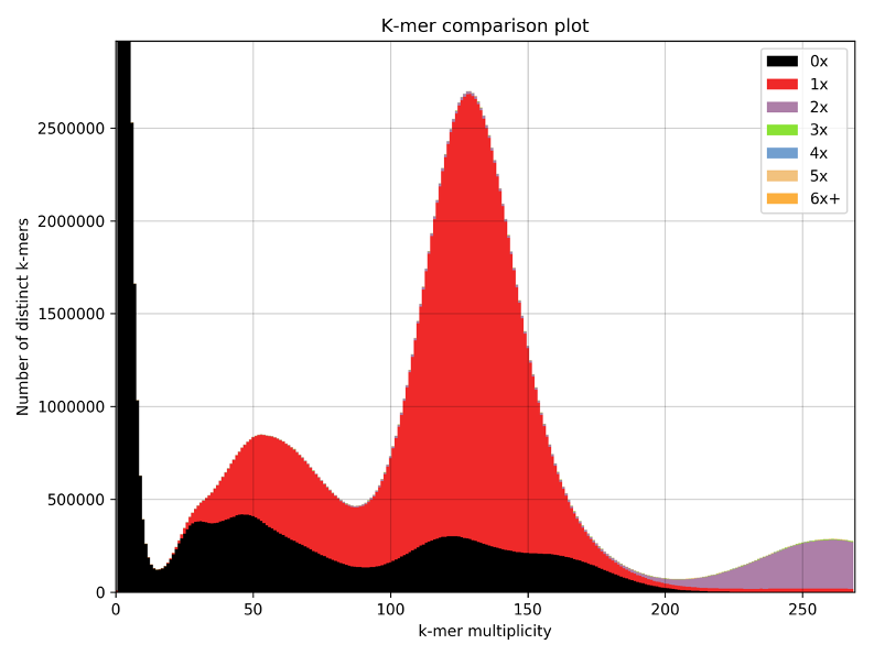
7) Regarding the section on palindromes and gene conversion
The authors screened all the published genomes for palindromes, including small blocks, to provide a more robust unbiased view. However, the result will be unbiased and robust if all the genomes compared were assembled using the same sequencing data (quality, coverage) and assembly program. While palindromes appear not to play a major role in the genome evolution of parthenogenetic animals since only few palindromes were detected among all lineages, mitotic (and meiotic) gene conversion is likely to take place in parthenogens and should indeed be studied among all the clades.
We agree with the reviewer that gene conversion might be one of the key aspects of asexual genome evolution. Our study merely pointed out that genomes of asexual animals do not show organisation in palindromes, indicating that palindromes might not be of general importance in asexual genome evolution. Note also that we clearly point out that these analyses are biased by the quality of the available genome assemblies.
8) Regarding the section on transposable elements
The authors are aware that the approach used may underestimate the TEs present in low copy numbers, therefore the comparison might underestimate the TE numbers in certain asexual groups.
Yes. We clearly explain this limitation in the manuscript. The currently available alternatives are based on assembled genomes, so the results are biased by the quality of the assemblies (and similarities to TEs in public databases) and our aim was to broadly compare genomes in the absence of assembly-generated biases.
9) Regarding the section on horizontal gene transfer. For the HGTc analysis, annotated genes were compared to the UniRef90 database to identify non-metazoan genes and HGT candidates were confirmed if they were on a scaffold containing at least one gene of metazoan origin. While this method is indeed interesting, it is also biased by the annotation quality and the length of the scaffolds which vary strongly between studies.
Yes, this is true and we explain many limitations in the supplemental information, but re-assembling and re-annotating all these genomes would be beyond reasonable computational possibilities.
10) Regarding the use of GenomeScope2.0
When homologues are very divergent (as observed in bdelloid rotifers) GenomeScope probably considers these distinct haplotypes as errors, making it difficult to model the haploid genome size and giving a high peak of errors in the GenomeScope profile. Moreover, due to the very divergent copies in A. vaga, GenomeScope indeed provides a diploid genome (instead of tetraploid).
For A. vaga, the heterozygosity estimated par GenomeScope2.0. on our new sequencing dataset is 2% (as shown in this paper). This % corresponds to the heterozygosity between k-mers but does not provide any information on the heterogeneity in heterozygosity measurements along the genome. A limitation of GenomeScope2.0. (which the authors should mention here) is that it is assuming that the entire genome is following the same theoretical k-mer distribution.
The model of estimating genome wide heterozygosity indeed assumes a random distribution of heterozygous loci and indeed is unable to estimate divergence over a certain threshold, which is the reason why we used genome assemblies for the estimation of divergence of homoeologs. Regarding estimates in all other genomes, the assumptions are unlikely to fundamentally change the output of the analysis. GenomeScope2 is described in detail in a recent paper (Ranallo-Benavidez et al. 2019), where the assumption that heterozygosity rates are constant across the genome is explicitly mentioned.
References
Engelstädter, Jan. "Asexual but not clonal: evolutionary processes in automictic populations." Genetics 206.2 (2017): 993-1009.
Flot, Jean-François, et al. "Genomic evidence for ameiotic evolution in the bdelloid rotifer Adineta vaga." Nature 500.7463 (2013): 453-457.
Handoo, Z. A., et al. "Morphological, molecular, and differential-host characterization of Meloidogyne floridensis n. sp.(Nematoda: Meloidogynidae), a root-knot nematode parasitizing peach in Florida." Journal of nematology 36.1 (2004): 20.
Suomalainen, Esko, Anssi Saura, and Juhani Lokki. Cytology and evolution in parthenogenesis. CRC Press, 1987.
Ranallo-Benavidez, Timothy Rhyker, Kamil S. Jaron, and Michael C. Schatz. "GenomeScope 2.0 and Smudgeplots: Reference-free profiling of polyploid genomes." BioRxiv (2019): 747568.
Jaron and collaborators provide a large-scale comparative work on the genomic impact of asexuality in animals. By analysing 26 published genomes with a unique bioinformatic pipeline, they conclude that none of the expected features due to the transition to asexuality is replicated across a majority of the species. Their findings call into question the generality of the theoretical expectations, and suggest that the genomic impacts of asexuality may be more complicated than previously thought.
The major strengths of this work is (i) the comparison among various modes and origins of asexuality across 18 independent transitions; and (ii) the development of a bioinformatic pipeline directly based on raw reads, which limits the biases associated with genome assembly. Moreover, I would like to acknowledge the effort made by the authors to provide on public servers detailed methods which allow the analyses to be reproduced. That being said, I also have a series of concerns, listed below:
We thank this reviewer for the relevant comments and for providing many constructive suggestions in the points below. We will take them into account for our final version of the manuscript.
1) Theoretical expectations
As far as I understand, the aim of this work is to test whether 4 classical predictions associated with the transition to asexuality and 5 additional features observed in individual asexual lineages hold at a large phylogenetic scale. However, I think that these predictions are poorly presented, and so they may be hardly understood by non-expert readers. Some of them are briefly mentioned in a descriptive way in the Introduction (L56 - 61), and with a little more details in the Boxes 1 and 2. However, the evolutive reasons why one should expect these features to occur (and under which assumptions) is not clearly stated anywhere in the Introduction (but only briefly in the Results & Discussion). I think it is important that the authors provide clear-cut quantitative expectations for each genomic feature analysed and under each asexuality origin and mode (Box 1 and 2). Also highlighting the assumptions behind these expectations will help for a better interpretation of the observed patterns.
We will clarify the expectations for non expert readers.
2) Mutation accumulation & positive selection
A subtlety which is not sufficiently emphasized to my mind is that the different modes of asexuality encompass reproduction with or without recombination (Box 2), which can lead to very different genetic outcomes. For example, it has been shown that the Muller's ratchet (the accumulation of deleterious mutations in asexual populations) can be stopped by small amounts of recombination in large-sized populations (Charlesworth et al. 1993; 10.1017/S0016672300031086). Similarly a new recessive beneficial mutation can only segregate at a heterozygous state in a clonal lineage (unless a second mutation hits the same locus); whereas in the presence of recombination, these mutations will rapidly fix in the population by the formation of homozygous mutants (Haldane's Sieve, Haldane 1927; 10.1017/S0305004100015644). Therefore, depending on whether recombination occurs or not during asexual reproduction, the expectations may be quite different; and so they could deviate from the "classical predictions". In this regard, I would like to see the authors adjust their conclusions. Moreover, it is also not very clear whether the species analysed here are 100% asexuals or if they sometimes go through transitory sexual phases, which could reset some of the genomic effects of asexuality.
Yes, the predictions regarding the efficiency of selection are indeed influenced by cellular modes of asexuality. Adding some details or at least a good reference would certainly increase the readability of the section. We thank the reviewer for this suggestion.
3) Transposable elements
I found the predictions regarding the amount of TEs expected under asexuality quite ambiguous. From one side, TEs are expected not to spread because they cannot colonize new genomes (Hickey 1982); but on the other side TEs can be viewed as any deleterious mutation that will accumulate in asexual genome due to the Muller's ratchet. The argument provided by the authors to justify the expectation of low TE load in asexual lineages is that "Only asexual lineages without active TEs, or with efficient TE suppression mechanisms, would be able to persist over evolutionary timescales". But this argument should then equally be applied to any other type of deleterious mutations, and so we won't be able to see Muller's ratchet in the first place. Therefore, not observing the expected pattern for TEs in the genomic data is not so surprising as the expectation itself does not seem to be very robust. I would like the authors to better acknowledge this issue, which actually goes into their general idea that the genomic consequences of asexuality are not so simple.
Indeed, the survivorship bias should affect all genomic features. Nothing that is incompatible with the viability of the species will ever be observed in nature. Perhaps the difference between Muller’s ratchet and the dynamics of accumulation of transposable elements (TEs) is that TEs are expected to either propagate very fast or not at all (Dolgin and Charlesworth 2006), while the effects of Muller’s ratchet are expected to vary among different populations and cellular mechanisms of asexuality. We will rephrase the text to better reflect the complexity of the predicted consequences of TE dynamics.
4) Heterozygosity
Due to the absence of recombination, asexual populations are expected to maintain a high level of diversity at each single locus (heterozygosity), but a low number of different haplotypes. However, as presented by the authors in the Box 2, there are different modes of parthenogenesis with different outcomes regarding heterozygosity: (1) preservation at all loci; (2) reduction or loss at all loci; (3) reduction depending on the chromosomal position relative to the centromere (distal or proximal). Therefore, the authors could benefit from their genome-based dataset to explore in more detail the distribution of heterozygosity along the chromosomes, and further test whether it fits with the above predictions. If the differing quality of the genome assemblies is an issue, the authors could at least provide the variance of the heterozygosity across the genome. The mode #3 (i.e. central fusions and terminal fusions) would be particularly interesting as one would then be able to compare, within the same genome, regions with large excess vs. deficit of heterozygosity and assess their evolutive impacts.
Moreover, the authors should put more emphasis on the fact that using a single genome per species is a limitation to test the subtle effects of asexuality on heterozygosity (and also on "mutation accumulation & positive selection"). These effects are better detected using population-based methods (i.e. with many individuals, but not necessarily many loci). For example, the FIS value of a given locus is negative when its heterozygosity is higher than expected under random mating, and positive when the reverse is true (Wright 1951; 10.1111/j.1469-1809.1949.tb02451.x).
We agree with the reviewer that the analysis of the distribution of heterozygosity along the chromosomes would be very interesting. However, the necessary data is available only for the Cape honey bee, and its analysis has been published by Smith et al. 2018. Calculating the probability distribution of heterozygosities would be possible, but it would require SNP calling for each of the datasets. Such an analysis would be computationally intensive and prone to biases by the quality of the genome assemblies.
5) Absence of sexual lineages
A second limit of this work is the absence of sexual lineages to use as references in order to control for lineage-specific effects. I do not agree with the authors when they say that "the theoretical predictions pertaining to mutation accumulation, positive selection, gene family expansions, and gene loss are always relative to sexual species [...] and cannot be independently quantified in asexuals." I think that this is true for all the genomic features analysed, because the transition to asexuality is going to affect the genome of asexual lineages relative to their sexual ancestors. This is actually acknowledged at the end of the Conclusion by the authors.
To give an example, the authors say that "Species with an intraspecific origin of asexuality show low heterozygosity levels (0.03% - 0.83%), while all of the asexual species with a known hybrid origin display high heterozygosity levels (1.73% - 8.5%)". Interpreting these low vs. high heterozygosity values is difficult without having sexual references, because the level of genetic diversity is also heavily influenced by the long term life history strategies of each species (e.g. Romiguier et al. 2014; 10.1038/nature13685).
I understand that the genome of related sexual species are not available, which precludes direct comparisons with the asexual species. However, I think that the results could be strengthened if the authors provided for each genomic feature that they tested some estimates from related sexual species. Actually, they partially do so along the Result & Discussion section for the palindromes, transposable elements and horizontal gene transfers. I think that these expectations for sexual species (and others) could be added to Table 1 to facilitate the comparisons.
Our statement "the theoretical predictions pertaining to mutation accumulation, positive selection, gene family expansions, and gene loss are always relative to sexual species [...] and cannot be independently quantified in asexuals." specifically refers to methodology: analyses to address these predictions require orthologs between sexual and asexual species. We fully agree that in addition to methodological constraints, comparisons to sexual species are also conceptually relevant - which is in fact one of the major points of our paper. We will clarify these points.
6) Regarding statistics, I acknowledge that the number of species analysed is relatively low (n=26), which may preclude getting any significant results if the effects are weak. However, the authors should then clearly state in the text (and not only in the reporting form) that their analyses are descriptive. Also, their position regarding this issue is not entirely clear as they still performed a statistical test for the effect of asexuality mode / origin on TE load (Figure 2 - supplement 1). Therefore, I would like to see the same statistical test performed on heterozygosity (Figure 2).
We will unify the sections and add an appropriate test everywhere where suited.
7) As you used 31 individuals from 26 asexual species, I was wondering whether you make profit of the multi-sample species. For example, were the kmer-based analyses congruent between individuals of the same species?
Unfortunately, some of the 31 individuals do not have publicly available reads (some of the root-knot nematode datasets are missing), others do not have sufficient quality (the coverage for some water flea samples is very low). Our analyses were consistent for the few cases where we have multiple datasets available.
References
Dolgin, Elie S., and Brian Charlesworth. "The fate of transposable elements in asexual populations." Genetics 174.2 (2006): 817-827.
Smith, Nicholas MA, et al. "Strikingly high levels of heterozygosity despite 20 years of inbreeding in a clonal honey bee." Journal of evolutionary biology 32.2 (2019): 144-152.
Reviewer #2 (Public review):
Summary:
The manuscript describes various conformational states and structural dynamics of the Insulin degrading enzyme (IDE), a zinc metalloprotease by nature. Both open and closed state structures of IDE have been previously solved using crystallography and cryo-EM which reveal a dimeric organization of IDE where each monomer is organized into N and C domains. C-domains form the interacting interface in the dimeric protein while the two N-domains are positioned on the outer sides of the core formed by C-domains. It remains elusive how the open state is converted into the closed state but it is generally accepted that it involves large-scale movement of N-domains relative to the C-domains. Authors here have used various complementary experimental techniques such as cryo-EM, SAXS, size-exclusion chromatography and enzymatic assays to characterize the structure and dynamics of IDE protein in the presence of substrate protein insulin whose density is captured in all the structures solved. The experimental structural data from cryo-EM suffered from high degree of intrinsic motion amongst the different domains and consequently, the resultant structures were moderately resolved at 3-4.1 Å resolution. Total five structures were generated in the originally submitted manuscript using cryo-EM. Another cryo-EM reconstruction (sixth) at 5.1Å resolution was mentioned after first revision which was obtained using time-resolved cryo-EM experiments. Authors have extensively used Molecular dynamics simulation to fish out important inter-subunit contacts which involves R668, E381, D309, etc residues. In summary, authors have explored the conformational dynamics of IDE protein using experimental approaches which are complimented and analyzed in atomic details by using MD simulation studies. The studies are meticulously conducted and lay ground for future exploration of protease structure-function relationship.
Comments after first peer-review:
The authors have addressed all my concerns, and have added new data and explanations in terms of time-resolved cryo-EM (Fig. 7) and upside simulations (Fig. 8) which in my opinion have strengthened the merit of the manuscript.
Author response:
The following is the authors’ response to the original reviews.
Reviewer #1 (Public review):
Summary:
Mancl et al. present cryo-EM structures of the Insulin Degrading Enzyme (IDE) dimer and characterize its conformational dynamics by integrating structures with SEC-SAXS, enzymatic activity assays, and all-atom molecular dynamics (MD) simulations. They present five cryo-EM structures of the IDE dimer at 3.0-4.1 Å resolution, obtained with one of its substrates, insulin, added to IDE in a 1:2 ratio. The study identified R668 as a key residue mediating the open-close transition of IDE, a finding supported by simulations and experimental data. The work offers a refined model for how IDE recognizes and degrades amyloid peptides, incorporating the roles of IDE-N rotation and charge-swapping events at the IDE-N/C interface.
Strengths:
The study by Mancl et al. uses a combination of experimental (cryoEM, SEC-SAXS, enzymatic assays) and computational (MD simulations, multibody analysis, 3DVA) techniques to provide a comprehensive characterization of IDE dynamics. The identification of R668 as a key residue mediating the open-to-close transition of IDE is a novel finding, supported by both simulations and experimental data presented in the manuscript. The work offers a refined model for how IDE recognizes and degrades amyloid peptides, incorporating the roles of IDE-N rotation and chargeswapping events at the IDE-N/C interface. The study identifies the structural basis and key residues for IDE dynamics that were not revealed by static structures.
Weaknesses:
Based on MD simulations and enzymatic assays of IDE, the authors claim that the R668A mutation in IDE affects the conformational dynamics governing the open-closed transition, which leads to altered substrate binding and catalysis. The functional importance of R668 would be substantiated by enzymatic assays that included some of the other known substrates of IDE than insulin such as amylin and glucagon.
We have included amyloid beta in our enzymatic assays, as shown in Figure 5D, and have updated the manuscript text accordingly. The R668A mutation results in a loss of dose-dependent competition with amyloid beta, but not with insulin. To further substantiate this unexpected finding, we plan to undertake a comprehensive biochemical characterization of the R668A mutation across a variety of substrates, followed by structural analysis of this mutant. However, these investigations are beyond the scope of the current study and, if successful, warrant a separate publication.
It is unclear to what extent the force field (FF) employed in the MD simulations favors secondary structures and if the lack of any observed structural changes within the IDE domains in the simulations - which is taken to suggest that the domains behave as rigid bodies - stems from bias by the FF.
We utilized the widely adopted CHARMM36 force field, whose parameters have been validated by thousands of previous studies. As shown in Figure 2A, our simulations reveal small but noticeable fluctuations in intradomain RMSD values. However, after careful examination, we found that these changes do not correspond to any biologically meaningful motions based on previously reported structural and biophysical characterizations of IDE (e.g., Shen et al., Nature 2006; Noinaj et al., PLOS One 2011; McCord et al., PNAS 2013; Zhang et al., eLife 2018, and references therein).
Reviewer #2 (Public review):
Summary:
The manuscript describes various conformational states and structural dynamics of the Insulin degrading enzyme (IDE), a zinc metalloprotease by nature. Both open and closed-state structures of IDE have been previously solved using crystallography and cryo-EM which reveal a dimeric organization of IDE where each monomer is organized into N and C domains. C-domains form the interacting interface in the dimeric protein while the two N-domains are positioned on the outer sides of the core formed by Cdomains. It remains elusive how the open state is converted into the closed state but it is generally accepted that it involves large-scale movement of N-domains relative to the C-domains. The authors here have used various complementary experimental techniques such as cryo-EM, SAXS, size-exclusion chromatography, and enzymatic assays to characterize the structure and dynamics of IDE protein in the presence of substrate protein insulin whose density is captured in all the structures solved. The experimental structural data from cryo-EM suffered from a high degree of intrinsic motion among the different domains and consequently, the resultant structures were moderately resolved at 3-4.1 Å resolution. A total of five structures were generated by cryo-EM. The authors have extensively used Molecular dynamics simulation to fish out important inter-subunit contacts which involve R668, E381, D309, etc residues. In summary, authors have explored the conformational dynamics of IDE protein using experimental approaches which are complemented and analyzed in atomic details by using MD simulation studies. The studies are meticulously conducted and lay the ground for future exploration of the protease structure-function relationship.
Reviewer #1 (Recommendations for the authors):
The manuscript reads well, however, there are minor details throughout that would tighten it up and, in some cases, make it easier to approach for a broader readership:
Abstract
(1) R668 is referred to by its one-letter code throughout the main text but referred to as arginine-668 in the abstract. The abstract should be corrected to R668.
This has been corrected.
(2) The authors should consider reordering the significance of their work as it is listed at the end of the abstract. As the work first and foremost "offers the molecular basis of unfoldase activity of IDE and provides a new path forward towards the development of substrate-specific modulators of IDE activity" these should come before "the power of integrating experimental and computational methodologies to understand protein dynamics".
We have revised abstract substantially to incorporate the new findings. Consequently, the sentence for "the power of integrating experimental and computational methodologies to understand protein dynamics" has been removed.
Main text
(1) Cryo-EM is consistently referred to as cryoEM throughout the text. The commonly accepted format for referring to cryogenic electron microscopy is cryo-EM. The authors are asked to consider revising the text accordingly.
The text has been revised.
(2) Introduction: The authors are asked to consider including a figure (panel) that provides the general reader with an overview of IDE architecture and topology as a point of reference in the introduction to understanding the pseudo symmetry in IDE, domains, and IDE-C relative to IDE-N, etc. This is relevant for reading most of the figures.
We have added a new figure 1 to provide the background and questions to be answered.
(3) The authors should consider renaming some of the headers in the results section to include the main conclusion. For instance, "CryoEM structures of IDE in the presence of a sub-saturating concentration of insulin" is not really helpful for the reader to understand the work, while "R668A mediates IDE conformational dynamics in vitro" is.
The headings have been altered in an effort to be more informative.
(4) It is unclear what the timescale for insulin cleavage is for IDE. Clearly, it is possible for the authors to capture an insulin-bound IDE from within the 7 million particles, but what is the chance of this? The authors emphasize the IDE:insulin ratio relative to previous experiments, but surely the kinetics would be the same in the two experiments that were presumably set up exactly the same way. In the context of this, the authors should disclose how concentrations were estimated experimentally. The authors are encouraged to touch upon the subject of time scales to tie up cryo-EM and enzyme experiments with MD simulations.
Both reviewers posted the question about time-scale relevant to IDE catalysis. In response to this request, we have revised the manuscript to address the relevance of key kinetic timescales. Specifically, we now discuss the open/closed transition (~0.1 second) and insulin cleavage (~2/sec), both established experimentally in prior studies (McCord et al PNAS 2013).
IDE concentrations were determined by spectrometry (Nanodrop and/or Bradford assay), and its purity was confirmed to be greater than 90% by SDS-PAGE. Insulin was purchased commercially, weighed, and dissolved in buffer, with its concentration subsequently verified using Nanodrop. Catalytically inactive IDE and insulin were mixed and incubated for at least 30 minutes. Given IDE’s low nanomolar affinity for insulin, and the sub-stoichiometric insulin concentrations used, sufficient time was allowed for insulin to bind IDE and remain bound.
To distinguish between IDE’s unfoldase and protease activities, all structural analyses were performed in the presence of EDTA, which chelates catalytic zinc, thereby inactivating IDE. This approach inhibits the enzyme’s catalytic cycle and allows us to capture the fully unfolded state of insulin bound to IDE in its closed conformation, representing the endpoint of the reaction. Under these conditions, the only meaningful kinetic parameter available for investigation was the unfolding of insulin by IDE.
To elaborate the interaction between IDE and insulin in the catalytically relevant time regime, we investigated IDE–insulin interactions within the millisecond time regime by rapidly mixing IDE with a large molar excess of insulin for approximately 120 milliseconds for the cryo-EM single particle analysis. Under these conditions, we observed that both IDE subunits in the dimer predominantly adopt open states, which are distinct from those previously reported. This observation suggests a potential mechanism of allostery in IDE function.
(5) It should be included in the main text that the data was processed with C1 symmetry and not just in Table 1. This is more useful information for understanding the study than the number of micrographs.
We have stated that the data was processed with C1 symmetry at the start of the results section.
(6) The authors should consider adding speculation on what the approximately 6 million particles that did not yield a high-resolution structure represent.
In cryo-EM single particle analysis, particle selection is typically performed automatically using software such as Relion. Due to the low signal-to-noise ratio, many “junk particles”—originating from contaminants such as ice, impurities, aggregates, or incomplete particles—are inevitably included along with the particles of interest. It is standard practice to filter out these junk particles during data processing. In our case, we estimate that the majority of the 6 million particles are likely junk. However, we cannot fully exclude the possibility that some of these particles may originate from IDE and carry potentially useful information about its conformational heterogeneity. Nonetheless, current cryo-EM single particle analysis methods face significant challenges in objectively recovering and interpreting such particles.
Reviewer #2 (Recommendations for the authors):
I have some minor comments regarding the manuscript which are given below.
(1) For O/O state, it will be great to see an explanation regarding why the values are dissimilar for 0.5 and 0.143 FSC.
All of our IDE structures (including previously published data) demonstrate a dip/plateau at moderate resolution in their FSCs. We interpret this an indicator of structural heterogeneity, as the dip/plateau is smallest in the pC/pC state, becomes larger when one of the subunits is open, and is largest when both subunits are open. Because both subunits within the O/O state are highly heterogeneous, the FSC dipped below the 0.5 threshold. Other states, such as the O/pO, display the same FSC trend, the dip remains slightly above the 0.5 threshold.
(2) O/pO state is moderately resolved at 4.1 Å, but this state is populated with many particles (328,870). Can the resolution be improved by more extensive sorting of heterogenous particles which intrinsically causes misalignment amongst particles?
Unfortunately, no. As shown by the local resolution maps in Figure 1-figure supplement 1, the primary source of misalignment is the IDE-N region in the open subunit. We have found that IDE-N is nearly unconstrained in its conformational flexibility in the open state, and does not appear to adopt discrete states, our attempts to better classify particles have failed. We speculate that this may be a failing in kmeans cluster based classification, and this is part of the driving force behind our exploration of advanced methods of heterogeneity analysis.
(3) Given the observation that capturing a substrate-bound open state is difficult, it can be assumed that the substrate capture in the catalytic cleft is a fast event. Please comment on the possible time frame of unfolding of substrate and catalysis. Can authors comment on any cryo-EM experiments that can deal with such a short time frame? If there is a possibility to include data from such experiments, then it may be considered.
This has been addressed in conjunction with the previous reviewer’s comment (see above). Specifically, we now discuss the open/closed transition (~0.1 second) and insulin cleavage (~2/sec), both established experimentally in prior studies. Additionally, we investigated IDE–insulin interactions by rapidly mixing IDE with a large molar excess of insulin for approximately 120 milliseconds for the cryo-EM single particle analysis. Under these conditions, we observed that both IDE subunits in the dimer predominantly adopt open states, which are distinct from those previously reported. This observation suggests a potential mechanism of allostery in IDE function.
(4) How long was incubation time after adding any substrates, such as insulin? Can different incubation times be tested to generate additional information regarding other conformational states that lie in between open and closed states?
The incubation time for IDE with insulin prior to cryo-EM grid freezing was approximately 30 minutes. We agree that it would be exciting to explore shorter time frames to identify new conformational states. As discussed above, we have rapidly mixed IDE with a large molar excess of insulin for approximately 120 milliseconds for the cryo-EM single particle analysis. Under these conditions, we observed that both IDE subunits in the dimer predominantly adopt open states, which are distinct from those previously reported. This observation suggests a potential mechanism of allostery in IDE function.
(5) A complex network of hydrogen bonding interaction initiated by R668 latching onto N-domain is mentioned in MD simulation studies but it is not clear why cryo-EM experiments did not capture such stabilized structures.
We believe that two main factors have prevented us from observing the hydrogen bonding network in our cryo-EM structures. The first factor is the requirement to freeze the sample in liquid ethane. According to the second law of thermodynamics, lowering the temperature reduces the effect of entropy. Our findings suggest that residue R668 interacts with several neighboring residues through a network of polar and electrostatic interactions, rather than being limited to a single partner. These interactions facilitate both the open-closed transitions and rotational movements between IDE-N and IDE-C. From a thermodynamic perspective, these interactions have both enthalpic and entropic components, and cooling the sample diminishes the entropic contribution. In line with this, we observe that the closed-state domains in our cryo-EM studies are positioned closer together than in our MD simulations, though not as tightly as in crystal structures of IDE. This implies that cryogenic data collection may constrain the interface between IDE-N and IDE-C, which can further alter the equilibrium for the network of R668 mediated interactions.
Secondly, our cryo-EM structures represent ensemble averages of tens to hundreds of thousands of particles. MD simulations indicate that IDE-N and IDE-C can rotate relative to one another, resulting in considerable variability in residue interactions. However, the level of particle density in our cryo-EM data does not permit sufficiently fine classification to resolve these differences. As a result, distinct hydrogen bonding networks are likely averaged out in the ensemble structure, particularly in the case of R668, which is indicated to interact with multiple neighboring residues in the conformation-dependent manner. This averaging effect may also contribute to our inability to achieve resolutions below 3 Å.
(6) Despite the observation that IDE is an intrinsically flexible protein, it seems probable that differently-sized substrates might reveal additional interaction networks formed by other novel key players apart from just R668. Will it be helpful to first try this computationally using MD simulations and then try to replicate this in cryo-EM experiments? If needed, additional simulation time may be added to the MD analysis. Please comment!
We agree that this is an exciting avenue to explore. Doubly so when considered in light of our R668A enzymatic results with amyloid beta. However, several challenges must be overcome before we can explore this direction effectively:
(1) We lack experimental knowledge of the initial interaction event between IDE and substrate. All substrate-bound IDE structures have been obtained after unfolding and positioning for cleavage has occurred. Without a solid foundational model for the initial interaction event between IDE and substrate, the interpretation of subsequent MD simulations is open to question.
(2) We have previously observed minimal effect of substrate on IDE in all-atom MD simulations. We believe that observable effects would require a much longer time scale than is currently achievable with all-atom MD, so have turned to Upside, a coarse-grained method to overcome these limitations, but Upside handles side chains with presumptive modeling, which prevent the identification of potential novel residue interactions.
(3) Due to the conformational heterogeneity present within IDE cryo-EM datasets, we struggle to obtain sufficient resolution to clearly identify side chain interactions at the domain interface (see response to 5).
Given these challenges, we plan to explore these directions in future manuscripts.
(7) What is the possibility of water interaction networks and dynamism in this network to contribute to the overall dynamics of the protein in the presence and absence of substrates? How symmetric these networks be in the four domains of dimeric IDE?
This is an interesting idea that we have begun to explore, but consider to be outside the scope of this work. Currently, we do not have any MD simulations containing substrate with explicit solvent (Upside uses implicit solvent), and solvent atoms were removed from our all-atom simulations prior to analysis to speed up processing. That being said, preliminary WAXS data suggests that there may be a difference in water interaction interfaces between WT and R668A IDE, and this is a lead we plan to pursue in future work.
(8) Line 214: Please fix the typo which wrongly describes closed = pO.
This is not a typo, but it is confusing. The pO state has previously been defined as the closed state of IDE lacking bound substrate as determined by cryo-EM. This differentiates the pO state from the pC state, where the pC state contains density indicative of bound substrate. As the MD simulations were conducted with the apo-state, the closed state the simulations were initialized from was the pO state structure, which represents the substrate-free closed state as determined by cryo-EM. We realize that this difference is probably unnecessary to the majority of readers, and have removed the (pO) specificity to avoid confusion.
(9) It is not clear why a cryo-EM structure was not attempted for the R668A mutant. If the authors have tried to generate such a structure, it should be mentioned in the manuscript. Such a structure should yield more information when compared to SAXS experiments.
We have not attempted to obtain a cryo-EM structure for the R668A mutant. Our SAXS analysis suggests a transition from a dominant O/pO state to a dominant O/O state. The O/O state is known to exhibit the highest degree of conformational heterogeneity, which severely limits structural insights. We are working to better handle the sample preparation of IDE and perform such analysis without the need to use Fab. We plan to further characterize IDE R668A biochemically and potentially explore other mutations that would provide insights in how IDE works. Armed with that, we will perform the structural analysis of such IDE mutant(s).
Reviewer #3 (Public review):
Summary:
Here, Bykov et al move the bi-genomic split-GFP system they previously established to the genome-wide level in order to obtain a more comprehensive list of mitochondrial matrix and inner membrane proteins. In this very elegant split-GFP system, the longer GFP fragment, GFP1-10, is encoded in the mitochondrial genome and the shorter one, GFP11, is C-terminally attached to every protein encoded in the genome of yeast Saccharomyces cerevisiae. GFP fluorescence can therefore only be reconstituted if the C-terminus of the protein is present in the mitochondrial matrix, either as part of a soluble protein, a peripheral membrane protein or an integral inner membrane protein. The system, combined with high-throughput fluorescence microscopy of yeast cells grown under six different conditions, enabled the authors to visualize ca. 400 mitochondrial proteins, 50 of which were not visualised before and 8 of which were not shown to be mitochondrial before. The system appears to be particularly well suited for analysis of dually localized proteins and could potentially be used to study sorting pathways of mitochondrial inner membrane proteins.
Strengths:
Many fluorescence-based genome-wide screen were previously performed in yeast and were central to revealing the subcellular location of a large fraction of yeast proteome. Nonetheless, these screens also showed that tagging with full-length fluorescent proteins (FP) can affect both the function and targeting of proteins. The strength of the system used in the current manuscript is that the shorter tag is beneficial for detection of a number of proteins whose targeting and/or function is affected by tagging with full length FPs.
Furthermore, the system used here can nicely detect mitochondrial pools of dually localized proteins. It is especially useful when these pools are minor and their signals are therefore easily masked by the strong signals coming from the major, nonmitochondrial pools of the proteins.
Weaknesses:
My only concern is that the biological significance of the screen performed appears limited. The dataset obtained is largely in agreement with several previous proteomic screens but it is, unfortunately, not more comprehensive than them, rather the opposite. For proteins that were identified inside mitochondria for the first time here or were identified in an unexpected location within the organelle, it remains unclear whether these localizations represent some minor, missorted pools of proteins or are indeed functionally important fractions and/or productive translocation intermediates. The authors also allude to several potential applications of the system but do little to explore any of these directions.
Comments on revisions:
The revised version of the manuscript submitted by Bykov et al addresses the comments and concerns raised by the Reviewers. It is a pity that the verification of the newly obtained data and its further biological exploration is apparently more challenging than perhaps anticipated.
Author response:
The following is the authors’ response to the original reviews.
Reviewer #1 (Public Review):
Summary:
The study conducted by the Schuldiner's group advances the understanding of mitochondrial biology through the utilization of their bi-genomic (BiG) split-GFP assay, which they had previously developed and reported. This research endeavors to consolidate the catalog of matrix and inner membrane mitochondrial proteins. In their approach, a genetic framework was employed wherein a GFP fragment (GFP1-10) is encoded within the mitochondrial genome. Subsequently, a collection of strains was created, with each strain expressing a distinct protein tagged with the GFP11 fragment. The reconstitution of GFP fluorescence occurs upon the import of the protein under examination into the mitochondria.
We are grateful for the positive evaluation. We would like to clarify that the bi-genomic (BiG) split-GFP assay was developed by the labs of H. Becker and Roza Kucharzyk by highly laborious construction of the strain with mtDNA-encoded GFP<sub>1-10</sub> (Bader et al, 2020).
Strengths:
Notably, this assay was executed under six distinct conditions, facilitating the visualization of approximately 400 mitochondrial proteins. Remarkably, 50 proteins were conclusively assigned to mitochondria for the first time through this methodology. The strains developed and the extensive dataset generated in this study serve as a valuable resource for the comprehensive study of mitochondrial biology. Specifically, it provides a list of 50 "eclipsed" proteins whose role in mitochondria remains to be characterized.
Weaknesses:
The work could include some functional studies of at least one of the newly identified 50 proteins.
In response to this we have expanded the characterization of phenotypic effects resulting from changing the targeting signal and expression levels of the dually localized Gpp1 protein and expanded the data in Fig. 3, panels H and I.
Reviewer #2 (Public Review):
The authors addressed the question of how mitochondrial proteins that are dually localized or only to a minor fraction localized to mitochondria can be visualized on the whole genome scale. For this, they used an established and previously published method called BiG split-GFP, in which GFP strands 1-10 are encoded in the mitochondrial DNA and fused the GFP11 strand C-terminally to the yeast ORFs using the C-SWAT library. The generated library was imaged under different growth and stress conditions and yielded positive mitochondrial localization for approximately 400 proteins. The strength of this method is the detection of proteins that are dually localized with only a minor fraction within mitochondria, which so far has hampered their visualization due to strong fluorescent signals from other cellular localizations. The weakness of this method is that due to the localization of the GFP1-10 in the mitochondrial matrix, only matrix proteins and IM proteins with their C-termini facing the matrix can be detected. Also, proteins that are assembled into multimeric complexes (which will be the case for probably a high number of matrix and inner membrane-localized proteins) resulting in the C-terminal GFP11 being buried are likely not detected as positive hits in this approach. Taking these limitations into consideration, the authors provide a new library that can help in the identification of eclipsed protein distribution within mitochondria, thus further increasing our knowledge of the complete mitochondrial proteome. The approach of global tagging of the yeast genome is the logical consequence after the successful establishment of the BiG split-GFP for mitochondria. The authors also propose that their approach can be applied to investigate the topology of inner membrane proteins, however, for this, the inherent issue remains that it cannot be excluded that even the small GFP11 tag can impact on protein biogenesis and topology. Thus, the approach will not overcome the need to assess protein topology analysis via biochemical approaches on endogenous untagged proteins.
Reviewer #3 (Public Review):
Summary:
Here, Bykov et al move the bi-genomic split-GFP system they previously established to the genomewide level in order to obtain a more comprehensive list of mitochondrial matrix and inner membrane proteins. In this very elegant split-GFP system, the longer GFP fragment, GFP1-10, is encoded in the mitochondrial genome and the shorter one, GFP11, is C-terminally attached to every protein encoded in the genome of yeast Saccharomyces cerevisiae. GFP fluorescence can therefore only be reconstituted if the C-terminus of the protein is present in the mitochondrial matrix, either as part of a soluble protein, a peripheral membrane protein, or an integral inner membrane protein. The system, combined with high-throughput fluorescence microscopy of yeast cells grown under six different conditions, enabled the authors to visualize ca. 400 mitochondrial proteins, 50 of which were not visualised before and 8 of which were not shown to be mitochondrial before. The system appears to be particularly well suited for analysis of dually localized proteins and could potentially be used to study sorting pathways of mitochondrial inner membrane proteins.
Strengths:
Many fluorescence-based genome-wide screens were previously performed in yeast and were central to revealing the subcellular location of a large fraction of yeast proteome. Nonetheless, these screens also showed that tagging with full-length fluorescent proteins (FP) can affect both the function and targeting of proteins. The strength of the system used in the current manuscript is that the shorter tag is beneficial for the detection of a number of proteins whose targeting and/or function is affected by tagging with full-length FPs.
Furthermore, the system used here can nicely detect mitochondrial pools of dually localized proteins. It is especially useful when these pools are minor and their signals are therefore easily masked by the strong signals coming from the major, nonmitochondrial pools of the proteins.
Weaknesses:
My only concern is that the biological significance of the screen performed appears limited. The dataset obtained is largely in agreement with several previous proteomic screens but it is, unfortunately, not more comprehensive than them, rather the opposite. For proteins that were identified inside mitochondria for the first time here or were identified in an unexpected location within the organelle, it remains unclear whether these localizations represent some minor, missorted pools of proteins or are indeed functionally important fractions and/or productive translocation intermediates. The authors also allude to several potential applications of the system but do little to explore any of these directions.
We agree with the reviewer that a single method may not be used for the construction of the complete protein inventory of an organelle or its sub-compartment. We suggest that the value of our assay is in providing a complementary view to the existing data and approaches. For example, we confirm the matrix localization of several proteins that were only found in the two proteomic data and never verified before (Vögtle et al, 2017; Morgenstern et al, 2017). Given that proteomics is a very sensitive technique and false positives are hard to completely exclude, our complementary verification is valuable.
Reviewer #1 (Recommendations for the authors):
In my opinion, the manuscript can be published as it is, and I would expect that future work will advance the functional properties of the newly found mitochondrial proteins.
We thank the reviewer for their positive evaluation
Reviewer #2 (Recommendations for the authors)
(1) Due to the localization of the GFP1-10 in the matrix, only matrix and IM proteins with C-termini facing the matrix can be detected, this should be added e.g. in the heading of the first results part and discussed earlier in the manuscript. In addition, the limitation that assembly into protein complexes will likely preclude detection of matrix and IM proteins needs to be discussed.
To address the first point, we edited the title of the first section to only mention the visualization of the matrix-facing proteome and remove the words “inner membrane”. We also clarified early in the Results section that we only consider the matrix-facing C-termini by extending the sentence early in the results section “To compare our findings with published data, we created a unified list of 395 proteins that are observed with high confidence using our assay indicating that their C-terminus is positioned in the matrix (Fig. 2 – figure supplement 1B-D, Table S1).” (P. 6 Lines 1-3). Concluding the comparison with the earlier proteomic studies we also added the sentence “Many proteins are missing because their C-termini are facing the IMS” (P.8 Line 2).
To address the second point concerning the possible interference of the complex assembly and protein detection by our assay, we conducted an additional analysis. The analysis takes advantage of the protein complexes with known structures where we could estimate if the C-terminus with the GFP<sub>11</sub> tag would be available for GFP1-10 binding. We added the additional figure (Figure 3 – figure supplement 2) and following text in the Results section (P.7 Lines 22-34):
“To examine the influence of protein complex assembly on the performance of the BiG Mito-Split assay we analyzed the published structures of the mitoribosome and ATP synthase (Desai et al, 2017; Srivastava et al, 2018; Guo et al, 2017) and classified all proteins as either having C-termini in, or out of, the complex. There was no difference between the “in” and “out” groups in the percentage observed in the BiG Mito-Split collection (Fig. 3 – figure supplement 2A) suggesting that the majority of the GFP11tagged proteins have a chance to interact with GFP1-10 before (or instead of) assembling into the complex. PCR and western blot verification of eight strains with the tagged complex subunits for which we observed no signal showed that mitoribosomal proteins were incorrectly tagged or not expressed, and the ATP synthase subunits Atp7, Atp19, and Atp20 were expressed (Fig. 3 – Supplement 2B). Atp19 and Atp20 have their C-termini most likely oriented towards the IMS (Guo et al, 2017) while Atp7 is completely in the matrix and may be the one example of a subunit whose assembly into a complex prevents its detection by the BiG Mito-Split assay.”
We also consider related points on the interference of the tag and the influence of protein essentiality in the replies to points 3) and 12) of these reviews.
(2) The imaging data is of high quality, but the manuscript would greatly benefit from additional analysis to support the claims or hypothesis brought forward by the authors. The idea that the nonmitochondrial proteins are imported due to their high sequence similarity to MTS could be easily addressed at least for some of these proteins via import studies, as also suggested by the authors.
The idea that non-mitochondrial proteins may be imported into mitochondria due to occasional sequence similarity was recently demonstrated experimentally by (Oborská-Oplová et al, 2025). We incorporate this information in the Discussion section as follows (P. 14 Lines 10-16):
“It was also recently shown that the r-protein uS5 (encoded by RPS2 in yeast) has a latent MTS that is masked by a special mitochondrial avoidance segment (MAS) preceding it (Oborská-Oplová et al, 2025). The removal of the MAS leads to import of uS5 into mitochondria killing the cells. The case of uS5 is an example of occasional similarity between an r-protein and an MTS caused by similar requirements of positive charges for rRNA binding and mitochondrial import. It remains unclear if other r-proteins have a MAS and if there are other mechanisms that protect mitochondria from translocation of cytosolic proteins.”
We also conducted additional analysis to substantiate the claim that ribosomal (r)-proteins are similar in their physico-chemical properties to MTS-containing mitochondrial proteins. For this we chose not to use prediction algorithms like TartgetP and MitoFates that were already trained on the same dataset of yeast proteins to discriminate cytosolic and mitochondrial localization. Instead, we extended the analysis earlier made by (Woellhaf et al, 2014) and calculated several different properties such as charge, hydrophobicity, hydrophobic moment and amino acid content for mitochondrial MTS-containing proteins, cytosolic non-ribosomal proteins, and r-proteins. The analysis showed striking similarity of r-proteins and mitochondrial proteins. We incorporate a new Figure 3 – figure supplement 3 and the following text in the Results section (P. 8 Lines14-22):
“Five out of eight proteins are components of the cytosolic ribosome (r-proteins). In agreement with previous reports (Woellhaf et al, 2014) we find that their unique properties, such as charge, hydrophobicity and amino acid content, are indeed more similar to mitochondrial proteins than to cytosolic ones (Fig. 3 – figure supplement 3). Additional experiments with heterologous protein expression and in vitro import will be required to confirm the mitochondrial import and targeting mechanisms of these eight non-mitochondrial proteins. The data highlights that out of hundreds of very abundant proteins with high prediction scores only few are actually imported and highlights the importance of the mechanisms that help to avoid translocation of wrong proteins (Oborská-Oplová et al, 2025).”
To further prove the possibility of r-protein import into mitochondria we aimed to clone the r-proteins identified in this work for cell-free expression and import into purified mitochondria. Despite the large effort, we have succeeded in cloning and efficiently expressing only Rpl23a (Author response image 1 A). Rpl23a indeed forms proteinase-protected fractions in a membrane potential-dependent manner when incubated with mitochondria. The inverse import dynamics of Rpl23a could be either indicative of quick degradation inside mitochondria or of background signal during the import experiments (Author response image 1.A). To address the r-protein degradation possibility, we measured how does GFP signal change in the BiG Mito-Split diploid collection strains after blocking cytosolic translation with cycloheximide (CHX). For this we selected Mrpl12a, that had one of the highest signals. We did not detect any drop in fluorescence signal for Rpl12a and the control protein Mrpl6 (Author response image 1 B). This might indicate the lack of degradation, or the degradation of the whole protein except GFP<sub>11</sub> that remains connected to GFP<sub>1-10</sub>. Due to time constrains we could not perform all experiments for the whole set of potentially imported r-proteins. Since more experiments are required to clearly show the mechanisms of mitochondrial r-protein import, degradation, and toxicity, or possible moonlighting functions (such as import into mitochondria derived from pim1∆ strain, degradation assays, fractionations, and analyses with antibodies for native proteins) we decided not to include this new data into the manuscript itself.
Author response image 1.
The import of r-proteins into mitochondria and their stability. (A) Rpl23 was synthesized in vitro (Input), radiolabeled, and imported into mitochondria isolated from BY4741 strain as described before (Peleh et al, 2015); the import was performed for 5,10, or 15 minutes and mitochondria were treated with proteinase K (PK) to degrade nonimported proteins; some reactions were treated with the mix of valinomycin, antimycin, and oligomycin (VAO) to dissipate mitochondrial membrane potential; the proteins were visualized by SDS-PAGE and autoradiography (B) The strains from the diploid BiG Mito-Split collection were grown in YPD to mid-logarithmic growth phase, then CHX was added to block translation and cell aliquots were taken from the culture and analyzed by fluorescence microscopy at the indicated time points. Scale bar is 5 µm.
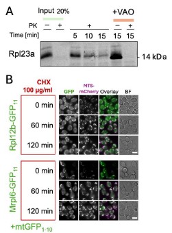
(3) The claim that the approach can be used to assess the topology of inner membrane proteins is problematic as the C-terminal tag can alter the biogenesis pathway of the protein or impact on the translocation dynamics (in particular as the imaging method applied here does not allow for analysis of dynamics). The hypothesis that the biogenesis route can be monitored is therefore far-reaching. To strengthen the hypothesis the authors should assess if the C-terminal GFP11 influences protein solubility by assessing protein aggregation of e.g. Rip1.
We agree with the reviewer that the tag and assembly of GFP<sub>1-10/11</sub> can further complicate the assessment of topology of the IM proteins that already have complex biogenesis routes (lateral transfer, conservative, and a Rip1-specific Bcs1 pathway). To emphasize that the assessment of the steady state topology needs to be backed up by additional biochemical approaches, we edited the beginning of the corresponding Results sections as follows (P. 11 Lines 2-6):
“Studying membrane protein biogenesis requires an accurate way to determine topology in vivo. The mitochondrial IM is one of the most protein-rich membranes in the cell supporting a wide variety of TMD topologies with complex biogenesis pathways. We aimed to find out if our BiG Mito-Split collection can accurately visualize the steady-state localization of membrane protein C-termini protruding into the matrix or trap protein transport intermediates” (inserted text is underlined).
The collection that we studied by microscopy is diploid and contains one WT copy of each 3xGFP<sub>11</sub>tagged gene. To assess the influence of the tag on the protein function we performed growth assays with haploid strains which have one 3xGFP<sub>11</sub>-tagged gene copy and no GFP<sub>1-10</sub>. We find that Rip13xGFP<sub>11</sub> displays slower growth on glycerol at 30˚C and even slower at 37˚C while tagged Qcr8, Qcr9, and Qcr10 grow normally (Author response image 2 A). Based on the growth assays and microscopy it is not possible to conclude whether the “Qcr” proteins’ biogenesis is affected by the tag. It may be that laterally sorted proteins are functional with the tag and constitute the majority while only a small portion is translocated into the matrix, trapped and visualized with GFP<sub>1-10</sub>. In case of Rip1 it was shown that C-terminal tag can affect its interaction with the chaperone Mzm1 and promote Rip1 aggregation (Cui et al, 2012). The extent of Rip1 function disruption can be different and depends on the tag. We hypothesize that our split-assay may trap the pre-translocation intermediate of Rip1 and can be helpful to study its interactors. To test this, we performed anti-GFP immune-precipitation (IP) using GFP-Trap beads (Author response image 2 B).
Author response image 2.
The influence of 3x-GFP11 on the function and processing of the inner membrane proteins. (A) Drop dilution assays with haploid strains from C-SWAT 3xGFP<Sub>11</sub> library on fermentative (YPD) and respiratory (YPGlycerol) media at different temperatures. (B) Immuno-precipitation with GFP-Trap agarose was performed on haploid strain that has only Rip1-3xGFP<sub>11</sub> and on the diploid strain derived from this haploid mated with BiG Mito-Split strain containing mtGFP<sub>1-10</sub> and WT untagged Rip1 using the lysis (1% TX-100) and washing protocols provided by the manufacturer; the total (T) and eluted with the Laemmli buffer (IP) samples were analyzed by immunoblotting with polyclonal rabbit antibodies against GFP (only visualizes GFP<Sub>11</sub> in these samples) and Rip1 (visualizes both tagged and WT Rip1). Polyclonal home-made rabbit antisera for GFP and Rip1 were kindly provided by Johannes Herrmann (Kaiserslautern) and Thomas Becker (Bonn); the antisera were diluted 1:500 for decorating the membranes.
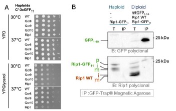
We find that the haploid strain with Rip1-3xGFP<sub>11</sub> contains not only mature (m) and intermediate (i) forms but also an additional higher Mw band that we interpreted as precursor that was not cleaved by MPP. WT Rip1 in the diploid added two more lower Mw bands: (m) and (i) forms of the untagged Rip1. IP successfully enriched GFP<sub>1-10</sub> fragment as visualized by anti-GFP staining. Interestingly only the highest Mw Rip1-3xGFP<sub>11</sub> band was also enriched when anti-Rip1 antibodies were used to analyze the samples. This suggests that Rip1 precursor gets completely imported and interacts with GFP<sub>1-10</sub> and can be pulled down. It is however not processed. Processed Rip1 is not interacting with GFP<sub>1-10</sub>. Based on the literature we expect all Rip1 in the matrix to be cleaved by MPP including the one interacting with GFP. Due to this discrepancy, we did not include this data in the manuscript. This is however clear that the assay may be useful to analyze biogenesis intermediates of the IM and matrix proteins. To emphasize this, we added information on the C-terminal tagging of Rip1 in the Results section (P. 11 Lines 18-20):
“It was shown that a C-terminal tag on Rip1 can prevent its interaction with the chaperone Mzm1 and promote aggregation in the matrix (Cui et al, 2012). It is also possible that our assay visualizes this trapped biogenesis intermediate.”
We also added a note on biogenesis intermediates in the Discussion (P. 14 Line 36 onwards):
“It is possible that the proteins with C-termini that are translocated into the IMS from the matrix side can be trapped by the interaction with GFP<sub>1-10</sub>. In that case, our assay can be a useful tool to study these pre-translocation intermediates.”
(4) The hypothesis that the method can reveal new substrates for Bcs1 is interesting, and it would strongly increase the relevance for the scientific community if this would be directly tested, e.g. by deleting BCS1 and testing if more IM proteins are then detected by interaction with the matrix GFP110.
we attempted to move the BiG Mito-Split assay into haploid strains where BCS1 and other factors can be deleted, however, this was not successful. Since this was a big effort (We cloned 10 potential substrate proteins but none of them were expressed) we decided not to pursue this further.
(5) The screening of six different growth conditions reflects the strength of the high-throughput imaging readout. However, the interpretation of the data and additional follow-up on this is rather short and would be a nice addition to the present manuscript. In addition, one wonders, what was the rationale behind these six conditions (e.g. DTT treatment)? The direct metabolic shift from fermentation to respiration to boost mitochondrial biogenesis would be a highly interesting condition and the authors should consider adding this in the present manuscript.
we agree with the reviewer that the analysis of different conditions is a strength of this work. However, we did not reveal any clear protein groups with strong conditional import and thus it was hard to select a follow-up candidate. The selection of conditions was partially driven by the technical possibilities: the media change is challenging on the robotic system; heat shock conditions make microscope autofocus unstable; library strain growth on synthetic respiratory media is very slow and the media cannot be substituted with rich media due to its autofluorescence. However, the usage of the spinning disc confocal microscope allowed us to screen directly in synthetic oleate media which has a lot of background on widefield systems due to oil micelles. We extended the explanation of condition choice as follows (P. 4 Line 34 onwards):
“The diploid BiG Mito-Split collection was imaged in six conditions representing various carbon sources and a diversity of stressors the cells can adapt to: logarithmic growth on glucose as a control carbon source and oleic acid as a poorly studied carbon source; post-diauxic (stationary) phase after growth on glucose where mitochondria, are more active and inorganic phosphate (Pi) depletion that was recently described to enhance mitochondrial membrane potential (Ouyang et al, 2024); as stress conditions we chose growth on glucose in the presence of 1 mM dithiothreitol (DTT) that might interfere with the disulfide relay system in the IMS, and nitrogen starvation as a condition that may boost biosynthetic functions of mitochondria. DTT and nitrogen starvation were earlier used for a screen with the regular C’-GFP collection (Breker et al, 2013). Another important consideration for selecting the conditions was the technical feasibility to implement them on automated screening setups.”
Reviewer #3 (Recommendations for the authors )
(6) This is a very elegant and clearly written study. As mentioned above, my only concern is that the biological significance of the obtained data, at this stage, is rather limited. It would have been nice if the authors explored one of the potential applications of the system they propose. For example, it should be relatively easy to analyze whether Cox26, Qcr8, Qcr9, or Qcr10 are new substrates of Bsc1, as the authors speculate.
we thank the reviewer for their positive feedback. We addressed the biological application of the screen by including new data on metabolite concentrations in the strains where Gpp1 N-terminus was mutated leading to loss of the mitochondrial form. We added panels H and I to Figure 4, the new Supplementary Table S2 and appended the description of these results at the end of the third Results subsection (P. 10 Lines 19-35). Our data now show a role for the mitochondrial fraction of Gpp1 which adds mechanistic insight into this dually localized protein.
We also were interested in the applications of our system to the study of mitochondrial import. However, the study of Cox26, Qcr8, Qcr9, and Qcr10 was not successful (also related to point 4, Reviewer #2). We thus decided to investigate the import mechanisms of the poorly studied dually localized proteins Arc1, Fol3, and Hom6 (related to Figure 4 of the original manuscript). To this end, we expressed these proteins in vitro, radiolabeled, and performed import assays with purified mitochondria. Arc1 was not imported, Fol3 and Hom6 gave inconclusive results (Author response image 3). Since it is known that even some genuine fully or dually localized mitochondrial proteins such as Fum1 cannot be imported in vitro post-translationally (Knox et al, 1998), we cannot draw conclusions from these experiments and left them out of the revised manuscript. Additional investigation is required to clarify if there exist special cytosolic mechanisms for the import of these proteins that were not reconstituted in vitro such as co-translational import.
Author response image 3.
In vitro import of poorly studies dually localized proteins. Arc1, Fol3, and Hom6 were cloned into pGEM4 plasmid, synthesized in vitro (Input), radiolabeled, and imported into mitochondria isolated from BY4741 strain as described before (Peleh et al, 2015); the import was performed for 5,10, or 15 minutes and mitochondria were treated with proteinase K (PK) to degrade non-imported proteins; some reactions were treated with the mix of valinomycin, antimycin, and oligomycin (VAO) to dissipate mitochondrial membrane potential. The proteins were separated by SDS-PAGE and visualized by autoradiography.
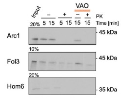
Minor comments:
(7) It is unclear why the authors used the six growth conditions they used, and why for example a nonfermentable medium was not included at all.
we address this shortcoming in the reply to the previous point 5 (Reviewer #2).
(8) Page 2, line 17 - "Its" should be corrected to "its".
Changed
(9) Page 2, line 25 to the end of the paragraph - the authors refer to the TIM complex when actually the TIM23 complex is probably meant. Also, it would be clearer if the TIM22 complex was introduced as well, especially in the context of the sentence stating that "the IM is a major protein delivery destination in mitochondria".
This was corrected.
(10) Page 5, line 35 - "who´s" should be corrected to "whose".
This was corrected.
(11) Page 9, line 5 - "," after Gpp1 should probably be "and".
This was corrected.
(12) Page 11 - the authors discuss in several places the possible effects of tags and how they may interfere with "expression, stability and targeting of proteins". Protein function may also be dramatically affected by tags - a quick look into the dataset shows that several mitochondrial matrix and inner membrane proteins that are essential for cell viability were not identified in the screen, likely because their function is impaired.
we agree with the reviewer that the influence of tags needs to be carefully evaluated. This is not always possible in the context of whole genomic screens. Sometimes, yeast collections (and proteomic datasets) can miss well-known mitochondrial residents without a clear reason. To address this important point we conducted an additional analysis to look specifically at the essential proteins. We indeed found that several of the mitochondrial proteins that are essential for viability were absent from the collection at the start, but for those present, their essentiality did not impact the likelihood to be detected in our assay. To describe the analysis we added the following text and a Fig. 3 – figure supplement 2. Results now read (P.7 Lines 8-21):
“Next, we checked the two categories of proteins likely to give biased results in high-throughput screens of tagged collections: proteins essential for viability, and molecular complex subunits. To look at the first category we split the proteomic dataset of soluble matrix proteins (Vögtle et al. 2017) into essential and non-essential ones according to the annotations in the Saccharomyces Genome Database (SGD) (Wong et al, 2023). We found that there was no significant difference in the proportion of detected proteins in both groups (17 and 20 % accordingly), despite essential proteins being less represented in the initial library (Fig. 3 – figure supplement 2A). From the three essential proteins of the (Vögtle et al. 2017) dataset for which the strains present in our library but showed no signal, two were nucleoporins Nup57 and Nup116, and one was a genuine mitochondrial protein Ssc1. Polymerase chain reaction (PCR) and western blot verification showed that the Ssc1 strain was incorrect (Fig. 3 – figure supplement 2B). We conclude that essential proteins are more likely to be absent or improperly tagged in the original C’-SWAT collection, but the essentiality does not affect the results of the BiG Mito-Split assay.”
Discussion (P. 13 Lines 23-26):
“We did not find that protein complex components or essential proteins are more likely to be falsenegatives. However, some essential proteins were absent from the collection to start with (Fig. 3 – figure supplement 2A). Thus, a small tag allows visualization of even complex proteins.”
From our data it is difficult to estimate the effect of tagging on protein function. We also addressed the effect of tagging Rip1 as well as performed growth assays on the tagged small “Qcr proteins” in the reply to point 3 (Reviewer #2). It is also difficult to estimate the effect of GFP<sub>1-10</sub> and <sub>11</sub> complex assembly on protein function since the presence of functional, unassembled GFP<sub>11</sub> tagged pool cannot be ruled out in our assay.
Other changes
Figure and table numbers changed after new data additions.
A sentence added in the abstract to highlight the additional experiments on Gpp1 function: “We use structure-function analysis to characterize the dually localized protein Gpp1, revealing an upstream start codon that generates a mitochondrial targeting signal and explore its unique function.”
The reference to the PCR verification (Fig. 3 – Supplement 2B) of correct tagging of Ycr102c was added to the Results section (P.8 Line 6), western blot verification added on.
Added the Key Resources Table at the beginning of the Methods section.
Small grammar edits, see tracked changes.
References:
Bader G, Enkler L, Araiso Y, Hemmerle M, Binko K, Baranowska E, De Craene J-O, Ruer-Laventie J, Pieters J, Tribouillard-Tanvier D, et al (2020) Assigning mitochondrial localization of dual localized proteins using a yeast Bi-Genomic Mitochondrial-Split-GFP. eLife 9: e56649
Cui T-Z, Smith PM, Fox JL, Khalimonchuk O & Winge DR (2012) Late-Stage Maturation of the Rieske Fe/S Protein: Mzm1 Stabilizes Rip1 but Does Not Facilitate Its Translocation by the AAA ATPase Bcs1. Mol Cell Biol 32: 4400–4409
Desai N, Brown A, Amunts A & Ramakrishnan V (2017) The structure of the yeast mitochondrial ribosome. Science 355: 528–531
Guo H, Bueler SA & Rubinstein JL (2017) Atomic model for the dimeric FO region of mitochondrial ATP synthase. Science 358: 936–940
Knox C, Sass E, Neupert W & Pines O (1998) Import into Mitochondria, Folding and Retrograde Movement of Fumarase in Yeast. J Biol Chem 273: 25587–25593
Morgenstern M, Stiller SB, Lübbert P, Peikert CD, Dannenmaier S, Drepper F, Weill U, Höß P, Feuerstein R, Gebert M, et al (2017) Definition of a High-Confidence Mitochondrial Proteome at Quantitative Scale. Cell Rep 19: 2836–2852
Oborská-Oplová M, Geiger AG, Michel E, Klingauf-Nerurkar P, Dennerlein S, Bykov YS, Amodeo S, Schneider A, Schuldiner M, Rehling P, et al (2025) An avoidance segment resolves a lethal nuclear–mitochondrial targeting conflict during ribosome assembly. Nat Cell Biol 27: 336–346
Peleh V, Ramesh A & Herrmann JM (2015) Import of Proteins into Isolated Yeast Mitochondria. In Membrane Trafficking: Second Edition, Tang BL (ed) pp 37–50. New York, NY: Springer
Srivastava AP, Luo M, Zhou W, Symersky J, Bai D, Chambers MG, Faraldo-Gómez JD, Liao M & Mueller DM (2018) High-resolution cryo-EM analysis of the yeast ATP synthase in a lipid membrane. Science 360: eaas9699
Vögtle F-N, Burkhart JM, Gonczarowska-Jorge H, Kücükköse C, Taskin AA, Kopczynski D, Ahrends R, Mossmann D, Sickmann A, Zahedi RP, et al (2017) Landscape of submitochondrial protein distribution. Nat Commun 8: 290
Woellhaf MW, Hansen KG, Garth C & Herrmann JM (2014) Import of ribosomal proteins into yeast mitochondria. Biochem Cell Biol 92: 489–498
Note: This response was posted by the corresponding author to Review Commons. The content has not been altered except for formatting.
Learn more at Review Commons
*We thank the reviewers for their valuable comments. A common suggestion by all reviewers was that the manuscript would benefit from restructuring. Following their recommendation we have restructured this manuscript to improve its readability. *
__Reviewer #1 (Evidence, reproducibility and clarity (Required)): __ The paper from Louka et al. studies the function of Cep104 during the development of Xenopus embryos. They perform overexpression and knock down experiments and address the consequences on neural tube closure, on ciliogenesis, and MT stability and on apical intercalation. There is a lot of data presented on a wide range of topics. While the data on MTs tracks reasonably well with other reports on Cep104, there are some concerns regarding the quality of some of the data and the interpretations based on the experimental results.
Specific Points: It is difficult to assess the effect on apical constriction with the data provided. Please show zoomed in higher mag images. Also this should be coupled with a quantification of cell number and proliferation rates, as it is possible that Cep104 mildly affects proliferation / cell division which could affect cell size. Overall this experiment is not really addressing apical constriction since there is no before and after data. Lots of things could affect apical surface area, most notably proliferation rates which one might predict would be affected by subtle changes to MT dynamics.
__Response: __Following the reviewer's recommendation we now show zoomed in higher magnification images to more clearly demonstrate the larger cell surface area in the morpholino injected neural plate compared to the control non-injected side in the same embryo. We agree with the reviewer that defects in cell proliferation could affect the cell size. If the effect of Cep104 on the cell surface area is caused by defects in cell proliferation, then we would expect this phenotype to persist in other tissues such as the ectoderm. However, we show that this phenotype is specific to the neural plate. On the other hand, if the cell surface area defect is caused by defects in apical constriction, we would expect this phenotype to be stage specific. Following the reviewer's recommendation, we compared the surface area of neuroectoderm cells before and after extensive apical constriction takes. The new data is shown in Figure S2. Our results show no difference in the surface area of neuroectoderm cells in control tracer injected and morpholino injected neuroepithelial cells at stage 13, before extensive apical constriction whereas significant differences are observed in stage 15 embryos during which cells undergo apical constriction. This data strengthens our conclusion that downregulation of Cep104 affects apical constriction.
"This defect was rescued with expression of exogenous human CEP104-GFP mRNA (300pg mRNA) (Figure 1D-E)." This was partially rescued as the control and the rescue are significantly different.
__Response: __We thank the reviewer for this important clarification. We edited the text to more clearly reflect our data.
I am unclear what is being depicted in Figure 1F and G. What is the intense red staining? Is that the blastopore? Which would imply that the stage of analysis is quite different between C and F which is concerning. The same stages should be used.
__Response: __This is an image of the anterior most region of a stage 15 embryo. Occasionally some embryos do display intense phalloidin staining at the neural plate. We replaced the image with a more clear one and moved this data to Figure S2C.
S1A has a boxed region as if there was going to be a zoomed in image, but there is not. It would be nice to see it zoomed in. While the localization is indeed at the base and tips of cilia the base looks too dispersed and big to be the basal body?
__Response: __Following the reviewer's recommendation we now show a zoomed in image of a primary cilium. The boxed area in figure S2A shows the cilium that was used to generate the fluorescence intensity profile plot shown in S2B. The Cep104 signal at the basal body is much stronger compared to the ciliary tip signal. Exposure that allows simultaneous detection of both the base and the tip signal results in overexposure of the signal at the base. This is consistent with observations in primary cilia in cell culture (please refer to Figure 4 in Frikstad et al. 2019 and Figure 3 in Yamazoe et al 2020).
In other systems the depletion of Cep104 decreases primary cilia length. While the authors claim that neural tube cilia are normal there is no quantification to support that and the provided image is hard to assess.
__Response: __Following the reviewer's recommendation we now show quantifications of the length of floor plate cilia (Figure S3C). Floor plate cilia are longer than the cilia found elsewhere in the neural tube. This inherent variability in the length of cilia will likely prevent the detection of small changes in the cilium length elicited by downregulation of Cep104. Therefore, we chose to examine the length of floor plate cilia only, in control and morpholino injected cells. Our results show that downregulation of Cep104 leads to the formation of shorter floor plate cilia which is in agreement with published data in other systems.
While the authors claim broad expression in humans and MO effects in cells without cilia, there is little data supporting the expression of Cep104 in the Xenopus cells being assayed (e.g. goblet cells).
__Response: __We agree with the reviewer that there is little evidence supporting the expression of Cep104 in Xenopus goblet cells. Cep104 is a very low abundance protein and thus very difficult to detect it at endogenous levels For example, Ryniawec et al. (2023) raised an antibody against Drosophila Cep104 that failed to detect the native (endogenous) protein via western blot or immunofluorescence, but successfully recognized the overexpressed (transgenic) Cep104. A proteomic study by Peshkin et al. 2019 showed that Cep104 levels remain relatively constant throughout Xenopus development suggesting that this protein is expressed ubiquitously. This data is shown in Figure 4 where we plot the relative expression levels of Cep104 along with two motile cilia specific genes: hydin and RSPH9.
The data in Figure 2 regarding the explants is difficult to understand and I think missing some key data. The text refers to the level of Gli increasing in the BF injected explants compared to uninjected explants, but the presentation of that is odd as the levels are normalized against uninjected rather than directly compared. And there are no stats for this key experiment. However, I think a bigger concern is the lack of information regarding the presence of cilia. While elongation and Sox2 expression are important they don't address if this tissue is similar to the neural tube in terms of cilia which is key to the interpretations.
__Response: __Following the reviewer's recommendation we changed the presentation of this data. GLI1 levels are now normalized to XBF2 injected explants. The results are the same, Gli1 levels are 25% lower in morphant XBF2 explants (ttest pWe understand the reviewer's concern regarding the presence of cilia in the explants. To our knowledge there are currently no reports on the presence of cilia in the neural ectoderm in Xenopus. We have made several attempts to determine if cilia are present in this tissue during neurulation. However, we have not been able to detect cilia based on immunofluorescence staining for acetylated tubulin and Arl13b in the neural ectoderm. We conclude from this experiment that downregulation of Cep104 negatively affects hedgehog signaling and it remains to be addressed whether this is due to defects in primary cilia.
The localization of Cep104 GFP in the epidermis and the neuroepithelium does not look similar as stated. Ones does not really see the punctate pattern in the neuroectoderm.
Response: We thank the reviewer for pointing this out. To more clearly present this data we now show a plot of the fluorescence profile of Cep104-GFP along cell-cell junctions to demonstrate the punctate localization in the neuroepithelium.
The experiments linking Cep104 to the tips of paused MTs is not particularly convincing. The depolymerization of MTs with nocodazole, will decrease all MTs as well as MT trafficking which could affect Cep104. Comparing this experiment with taxol treatment to stabilize MTs (and decrease dynamics) would be more convincing. Plus the image provided does not support the claim that the leftover EMTB is marked with Cep104.
__Response: __Following the reviewer's recommendation we have examined the effect of taxol on the density of Cep104 apical puncta. We injected embryos with CEP104-GFP and EMTB-scarlet and exposed them to 20 μm taxol and imaged them live at stage 38. Embryos non treated with taxol served as the control. As shown in Figure S4 treatment with taxol led to an increase in the density of Cep104 puncta. This further supports our conclusion that Cep104 localizes to the ends of stable or paused microtubules. We also revised Figure 5 to more clearly show that Cep104 remains associated with the ends of nocodazole resistant EMTB labeled microtubules.
The data in Figure 6 is very difficult to interpret / believe. The quantified effects on MTs are pretty subtle (which is fine...that is why you quantify), but the massive experimental variability questions the meaningfulness of those quantifications. In Fig 6B There are cells with lots of MTs right next to cells with no MTs and both have similar expression levels of Cep104. The staining just doesn't look consistent enough to accurately quantify. Also the effect of Nocodozole on MT stability is quite rapid, on the order of seconds to minutes, it is unclear what ON treatment with nocodazole would even be measuring since in that time there would be lots of secondary effects.
__Response: __We thank the reviewer for this comment. Some cells in the epidermis lack apical microtubules as the reviewer correctly points out. Cells without strong apical microtubule staining are seen in both control and morpholino injected cells. Here we quantified the number of control and morphant cells per embryo that lack apical microtubules (DMSO treated embryos). Our results show that similar numbers of control and morphant cells per embryo appear to lack apical microtubules. We think that the heterogeneity in tubulin signal is not an artifact of immunofluorescence staining since these cells are adjacent to cells with clear tubulin staining. Although the source of this variability is still unknown, the fact that an equal number of control and morphant cells show this phenotype suggests that this is unlikely to be linked to the injections or drug treatment. Those cells were excluded from the quantifications shown in Figures 6C and 6D It is possible that these cells are preparing to enter mitosis.
We think that the reviewer refers to the acute effects of nocodazole seen in cell cultures. However, in Xenopus tadpoles we didn't observe any effect on microtubules after short nocodazole treatment at low temperatures.
The authors propose that overexpressing Cep104 would lead to stabilized MTs which is a reasonable hypothesis, however, they test this in multiciliated cells that already have a ton of acetylated MTs. If their hypothesis is correct it should lead to an increase in acetylated tubulin in non multiciliated cells which don't have much to begin with. This would be a marked improvement as the side projection quantification seems a little suspect as the analysis requires a precises ROI that eliminates the strong cilia acetylation staining. While I believe that could be done, the image provided looks as if it might cut off some of the apical surface which highlights the challenge.
__Response: __Following the reviewer's recommendation, we examined the effect of Cep104 overexpression in non-MCCs on Xenopus epidermis. We show in Figure 7 that overexpression of Cep104 leads to a significant increase in the levels of acetylated tubulin in the cytoplasm of non-MCCs. We also show that overexpression of GFP alone did not have an effect on microtubule acetylation (Figure S5A). We moved the data on the cytoplasmic levels of acetylated microtubules in MCCs to figure S5B. We would like to clarify that the ROI to mark the cell body of MCCs was drawn right below the apical phalloidin signal to ensure that no signal derived from motile cilia will be included in the quantifications. A more detailed explanation of the quantification methods is included in this revised manuscript.
Minor: Overall the color choice of images does not conform to the color blind favorable options that are becoming standard in the field. Also to the extent possible the colors should be consistent (e.g. Fig 4 A Cep104-GFP is green but in B it is red).
__Response: __We thank the reviewer for this comment. We have changed the color choices in the figures to conform to the color blind.
The recent Xenopus Cep104 paper was referenced with two references, and the wording of those two sentences was redundant.
__Response: __We thank the reviewer for this comment. We edited the text accordingly.
__Reviewer #2 (Evidence, reproducibility and clarity (Required)): __ This study by Louka et al., investigates the function of Cep104, a protein associated with Joubert syndrome, in Xenopus. Several aspects are studied at different scales. Loss of function of this protein suggests a role in neural tube closure, apical constriction, and HH signaling. Moving on in the study, the authors investigate the localization of Cep104 in the primary cilia of the neural tube before focusing on its localization in multiciliated cells. They then look at the consequences of loss of function on motile cilia and conclude that it plays a role in the length of the distal segment. They then show an association of Cep104 with cytoplasmic microtubules in non-multiciliated cells of the Xenopus epidermis. They then analyze the function of Cep104 on these microtubules and show that loss of Cep104 function increases the speed of EB1 comets. They then looked at the impact of loss of function on microtubule stability and finally the impact of gain of function. Finally, they returned to the multiciliated cells and described an intercalation defect that correlated with decreases in acetylated tubulin. I think that certain controls are missing and that the choice of illustrations should be reconsidered (better quality, appropriate zoom). In terms of form, the text is not easy to read and the manuscript would benefit from reformatting to highlight the logical links between the different experiences and avoid a catalog-like effect. I would advise the authors to revise their introduction to make it less disjointed and guide readers toward the questions addressed by the manuscript.
Response: We thank the reviewer for the constructive criticism. We have revised the introduction to make it easier to read.
Below are specific comments and remarks: Figure 1: Why the conclusion is a "delay" in neural tube closure? At what stage is this analyzed? Is there a recovery of NT closure at later stage? A: I would suggest to provide control picture of non-injected and tracer only injected embryos. B: Statistics are missing on the graph D: mention what was injected instead of "+ rescue". Close up picture would allow a better appreciation of the differences in surface area.
Response: We thank the reviewer for this comment. The image shown in Figure 1A is from late neurula embryos, stage 18. We conclude that it is a delay in neural tube closure because the neural tube does close and the embryos develop to tailbud stages. To demonstrate the delay in neural tube closure we now include a time lapse sequence of a neurula stage embryo injected with the morpholino unilaterally which shows that the morpholino injected side moves towards the midline slower compared to the control uninjected side (movie 1). We also included a representative image of the dorsal side of a tailbud embryo injected unilaterally with the CEP104 morpholino to show that the neural tube has closed and the embryos develop to tailbud stages (figure S1D).
Following the reviewer's recommendation, we also show images of embryos injected unilaterally with the tracer alone (Figure S2), we included the statistical analysis for graph 1D, revised image 1D to show that the embryo is injected with the morpholino and CEP104-GFP and provide close ups to allow for better appreciation of the differences in surface area.
Figure S1: To illustrate the claim that cilia are not affected, it would be good to show injection of tracer alone and compare to tracer + morpholino. Also, to provide a measure of the cilia size.
__Response: __Following the reviewer's recommendation we quantified the length of floor plate cilia in the neural tube of control and morpholino injected embryos. As explained in our response to a comment by reviewer 1, the floor plate cilia are longer than the cilia found elsewhere in the neural tube. This inherent variability in the length of cilia will likely prevent the detection of small changes in the cilium length elicited by downregulation of Cep104. Therefore, we chose to examine the length of floor plate cilia only in control and morpholino injected cells. Our results show that downregulation of Cep104 leads to the formation of shorter floor plate cilia which is in agreement with published data in other systems (Figure S3C).
Figure 2: Please provide pictures to illustrate graph D.
__Response: __The graph in Figure 2D shows RT-qPCR results for CEP104 in BF2 and BF2 and morpholino injected explants as compared to non-injected explants. We do not have a working antibody that would allow us to show the downregulation at the protein level.
Figure 5: "Interestingly, most of the nocodazole-resistant stable microtubules were positive for Cep104 (Figure 5C, arrows). " The variation in density of Cep104-GFP signal is not visible on the pictures provided in C. I would suggest to show higher magnifications. Also, in the DMSO treated picture the Cep104GFP signal looks really different when compared to Cep104-GFP signal shown in B. Arrows should be reported on all channels. However, it not clear what we should see with this arrows. 5C: it seems that in nocodazole treated condition the Cep104-GFP is at the cilia base in MCCs which is different from the DMSO control condition. The basal body signal was not seen in the figure 3A which analyze the localization of Cep104-GFP in MCCs. Why not comment on this? Is it a phenotype on MCCs ?
Response: __Following the reviewer's recommendation, we now show higher magnifications of the images shown in Figure 5C. We removed the arrows as most reviewers found them confusing. To demonstrate the presence of Cep104 at the ends of nocodazole resistant EMTB labeled microtubules we show zoomed images and a representative fluorescence intensity profile plot. __Figure 5B shows an image of a non-MCC whereas Figure 5C shows a larger area on the tadpole epidermis which includes both MCCs and non-MCCs. We thank the reviewer for pointing out that the localization of Cep104 in 5C looks different from 3A. We do not think this is a phenotype on MCCs. In Figure 3A we imaged only the tips of cilia which is why it looks different from 5C in which we imaged the apical surface of the cells as well. We disagree with the reviewer regarding the comment '5C: it seems that in nocodazole treated condition the Cep104-GFP is at the cilia base in MCCs which is different from the DMSO control condition'. The basal body localization of Cep104 is shown in the DMSO image as well. We hope that it will be clear in this revised figure.
Figure 6: Intriguingly, morphant non-MCCs have significantly more mean β-tubulin signal compared to control non-MCCs in embryos treated with DMSO (Figure 6C). impossible to appreciate on the figures. Please specify on the figure what is considered as a morphant non-MCC versus a control non-MCC. The membrane-cherry positive cells (supposedly morphant? it has to be clarified show very heterogenous tubulin expression) If the point here is to show that microtubules are more sensitive to nocodazole in morphant cells as compared to control. I would suggest to show all conditions on a same graph. At least annotate more the graph for a self-explanatory figure (DMSO , Nocodazole).
__Response: __We agree with the reviewer that it impossible to appreciate the difference in β-tubulin signal between control and morphant non-MCCs. Based on the quantifications of mean β-tubulin fluorescence intensity there is 5% difference in the fluorescence intensity between the two groups. Statistical analysis using t-test shows that although very small, this difference is statistically significant which is why we mention it in the manuscript. We have removed this statement and data from the revised manuscript because this is a very subtle phenotype, and it is beyond the scope of this experiment.
Following the reviewer's recommendation, we clarify that mem-cherry positive cells contain the morpholino and mem-cherry negative cells are the control cells. We marked with a white asterisk the morphant non-MCCs. To address the heterogenous tubulin levels we provide quantifications which show that a similar number of control and morphant cells appear to lack microtubules. We think that the heterogeneity in tubulin signal is not an artifact of immunofluorescence staining since these cells are adjacent to cells with clear tubulin staining. Although the source of this variability is still unknown, the fact that an equal number of control and morphant cells show this phenotype suggests that this is unlikely to be linked to the injections or drug treatment. Those cells were excluded from the quantifications shown in figure 6. It is possible that these cells are preparing to enter mitosis. The reviewer is correct; the point of this experiment is to examine the effect of Cep104 downregulation on the sensitivity of microtubules to nocodazole. To more clearly present the results of this experiment we normalize the β-tubulin fluorescence Intensity in morphant cells to the one in control cells in the same embryo and we compare the normalized intensity in DMSO and nocodazole treated embryos.
Figure 7: Statistics are missing on Graph B
__ ____Response: __Following the reviewer's recommendation, we added the statistics on the graph.
Comment on the text: "Cep104 signal shows the characteristic two dot pattern in motile cilia (Figure 3A) that was also observed in a recent study using Xenopus Cep10465 and in the cilia of Tetrahymena50. This is in agreement with a recent study showing the characteristic two dot pattern for Xenopus Cep104 as well66 " ref 65 and 66b are the same (Hong et al., preprint)
__ ____Response: __We thank the reviewer for pointing this out. We edited the text to avoid repetition and corrected the references.
"This data suggests that downregulation of CEP104 affects the stability of cytoplasmic microtubules." I would suggest a more precise conclusion by stating how is it affected? More stable? Less stable? Important for the follow-up demonstration.
__ _Response: _We edited the text according to the reviewer's recommendation to precisely conclude that downregulation of Cep104 makes cytoplasmic microtubules less stable. __
Movies: Please annotate properly movie 2 and 3 so the reader can know what he/she is looking.
__Response: __Following the reviewer's comment, we revised the movie annotations to help the reader know what they are looking.
__Reviewer #3 (Evidence, reproducibility and clarity (Required)): __ The manuscript entitled "Ciliary and non-ciliary functions of Cep104 in Xenopus" by Louka et al. investigate roles for the centriole and cilia tip protein Cep104 in Xenopus embryos. The authors show that depletion of Cep104 prevents neural tube closure due to inefficient apical constriction of neural cells and defective hedgehog signaling. Cep104 depletion also resulted in structural and functional ciliary defects in multi-ciliated cells. Surprisingly, the authors discover a role for Cep104 in stabilizing cytoplasmic microtubules in non-ciliated and multi-ciliated cells. Reduced microtubule stability in Cep104-depleted cells correlated with reduced apical intercalation of multi-ciliated cells in the epidermis.
Overall, I find this manuscript difficult to understand because the experiments lack description of the findings within a normal developmental context and the findings are not developed into a cohesive narrative. I do find the study to be potentially impactful as the authors characterize Cep104 in a novel system (previous peer-reviewed studies have investigated Cep104 in human cell lines, Drosophila, zebrafish, Tetrahymena, and Chlamydomonas) with disease-relevant biology (neural development); however, mechanistic links are not properly explored. Over the course of their investigation, the authors made the novel finding that Cep104 controls the dynamics of cytoplasmic microtubules. However, this is not directly tested and potential pleiotropic effects of the developmental defects caused by Cep104 depletion confound the results.
Response: We thank the reviewer for their comments. We tried to address this by restructuring the manuscript to describe the results in more detail within a normal developmental context.
Major Critiques: The developmental context of experiments is not made clear. The authors use different tissues at varying developmental stages to perform experiments. However, these findings are not explored in depth and, therefore, the manuscript does not advance our understanding of Cep104's role in any of the processes explored.
__ ____Response:__ We thank the reviewer for their comment. We took advantage of different tissues during Xenopus development to understand the cellular and molecular function of this protein in vivo. In this manuscript we show that Cep104 is involved in neural tube closure likely through its effect on apical constriction. Our data show that Cep104 is important for the stability of cytoplasmic microtubules and this is further demonstrated through its role in apical intercalation of multiciliated cells, a process known to depend on stable microtubules. Although our data do not advance our understanding on developmental processes such as apical constriction and MCC apical intercalation, they do improve our understanding of how Cep104 impacts cytoplasmic microtubules which has not been addressed in vivo yet.
While the potential role of Cep104 in cytoplasmic microtubule regulation is intriguing, the experiments in the manuscript do not directly test this function. Because Cep104 depletion appears to have a profound developmental effect, it is difficult to interpret changes to EB1 velocity as directly attributed to Cep104 function. Additionally, the only evidence for Cep104 localization occurs in cells overexpressing human Cep104. The authors must directly visualize endogenous Cep104 to conclude microtubule or membrane localization, which they can also use to demonstrate Cep104 depletion in the morpholino experiments. Additionally, the assertion that Cep104 is binding plus-ends of cytoplasmic microtubules is not experimentally supported.
__ ____Response: __Unfortunately, we cannot directly visualize endogenous Cep104 because there is no commercially available antibody that works in Xenopus. Cep104 is a very low abundance protein, and this is highlighted in the study by John M.Ryniawec et al. 2023, where they generated an antibody against the drosophila Cep104 which detected the GFP-tagged DmCep104 but failed to detect the endogenous protein. Given that the ciliary and basal body signal of Cep104 represents the cumulative signal from nine microtubules, one can appreciate the difficulty of observing the Cep104 signal in individual microtubules. None of the commercially available Cep104 antibodies that we have tested worked against the Xenopus protein in immunofluorescence or western blot experiments. We agree with the reviewer that we do not experimentally test the binding of Cep104 to the microtubule plus-end. This has been demonstrated by others. In Jiang et al. 2012 it was showed that GFP-Cep104 co-immunoprecipitates with GST-EB1 but not with GST-EB1 that lacks the tail which contains the SxIP binging motif. In Yamazoe et al. 2020 study it was shown that exogenous Cep104 co-immunoprecipitates with exogenous EB1 and Cep104 with mutated SxIP motif (SKNN) fails to co-immunoprecipitate with EB1. This shows that Cep104 interacts with EB1 through its SxIP motif. In addition, overexpression of Cep104 recruits Cep97 to microtubule tips suggesting that it acts as a +TIP protein. A recent study by Saunders et al. 2025 showed that in in vitro microtubule reconstitution assays, Cep104 could not autonomously bind the microtubule plus-end at low concentrations but in the presence of EB3 it could bind the microtubule plus-end and block microtubule polymerization at the same low concentration. This shows that Cep104 interacts with EB3, localizes to the microtubule plus-end and affects its dynamics in vitro. We added this information in the manuscript to more clearly show that the interaction of Cep104 and EB proteins is well documented. We anticipate that this interaction will hold true in all cell types where the two proteins are co-expressed.
Additional Critiques: Figure S1. I only see the emergence of a shorter product after Cep104 depletion. Should PCR using Exon5-7 still work in successful knockdown? If not, then it is unclear what was quantified to determine Cep104 depletion as morpholino bands appear no different than control.
__ ____Response: __We thank the reviewer for this comment. PCR using exon5-7 will not work when splice blocking by the morpholino takes place. This is a knockdown approach and the efficiency of the morpholino is about 90%. Upon completion of the RT-qPCR cycle the samples were analyzed by gel electrophoresis to demonstrate that 1) alternative splicing took place (see two products with exon 3-7 primers) and 2) the presence of a single product for all primer sets used.
Figure 1A. Is this an example of an open or closed NTC? Show data used to determine the statement "no difference during convergent extension".
__ ____Response: __This is an example of an embryo that was unilatterally injected with the morpholino. The left side is the control non-injected side and the right side is the morpholino injected. We added this information on the figure to make it more self-explanatory. In Figure 2 the elongation of the BF2 injected explants is due to convergent extension. The statement "no difference during convergent extension" was removed from the revised manuscript.
Figure S2C. What does "Does not effect formation of cilia" mean? Does Cep104 depletion does not effect number, length, etc? Show quantitation used to determine this?
__ ____Response:__ Following the reviewer's recommendation, we quantified the length of floor plate cilia in control and morpholino injected embryos. As mentioned in our response to reviewer 1 and 2, floor plate cilia are longer than the cilia found elsewhere in the neural tube. This inherent variability in the length of cilia will likely prevent the detection of small changes in the cilium length elicited by downregulation of Cep104. Therefore, we chose to examine the length of floor plate cilia only, in control and morpholino injected cells. Our results show that downregulation of Cep104 leads to the formation of shorter floor plate cilia which is in agreement with published data in other systems.
Figure 5B. Along with strong Cep104 localization to membranes, there also appears to be strong EMTB localization. Is this also present in beta-tubulin immunostaining? Are these localizing to a cortical population of microtubules or to the membrane?
__ ____Response: __We thank the reviewer for their comment. The Cep104 puncta at the cell periphery, are reduced/lost upon nocodazole treatment thus we conclude that Cep104 localizes to microtubules and not the cell membrane (Figure 5C, zoomed images). Of course, we cannot exclude the possibility that microtubules are required to target CEP104 to the plasma membrane. We edited the text to clearly state this conclusion.
Figure 6C and 6D. These two panels have the same labels. The authors should denote that 6D is in nocodazole-treated explants.
__ ____Response:__ We thank the reviewer for this comment. We edited this figure to more clearly present the results of this experiment: We normalized the β -tubulin levels in morphant cells to that of control cells in the same embryo (mosaic morphant embryos were used in this experiment). The graph shows the mean normalized β -tubulin levels per embryo treated with DMSO or nocodazole.
Figure 7. What are Cep104 levels at stage 18-19?
__ ____Response: __Following the reviewer's comment we now show the Cep104 protein expression levels during Xenopus development as reported on Xenbase (Figure 4). Cep104 is expressed at low levels from gastrulation to tailbud stages (Figure 4D).
Note: This preprint has been reviewed by subject experts for Review Commons. Content has not been altered except for formatting.
Learn more at Review Commons
The manuscript entitled "Ciliary and non-ciliary functions of Cep104 in Xenopus" by Louka et al. investigate roles for the centriole and cilia tip protein Cep104 in Xenopus embryos. The authors show that depletion of Cep104 prevents neural tube closure due to inefficient apical constriction of neural cells and defective hedgehog signaling. Cep104 depletion also resulted in structural and functional ciliary defects in multi-ciliated cells. Surprisingly, the authors discover a role for Cep104 in stabilizing cytoplasmic microtubules in non-ciliated and multi-ciliated cells. Reduced microtubule stability in Cep104-depleted cells correlated with reduced apical intercalation of multi-ciliated cells in the epidermis.
Overall, I find this manuscript difficult to understand because the experiments lack description of the findings within a normal developmental context and the findings are not developed into a cohesive narrative. I do find the study to be potentially impactful as the authors characterize Cep104 in a novel system (previous peer-reviewed studies have investigated Cep104 in human cell lines, Drosophila, zebrafish, Tetrahymena, and Chlamydomonas) with disease-relevant biology (neural development); however, mechanistic links are not properly explored. Over the course of their investigation, the authors made the novel finding that Cep104 controls the dynamics of cytoplasmic microtubules. However, this is not directly tested and potential pleiotropic effects of the developmental defects caused by Cep104 depletion confound the results.
Major Critiques:
The developmental context of experiments is not made clear. The authors use different tissues at varying developmental stages to perform experiments. However, these findings are not explored in depth and, therefore, the manuscript does not advance our understanding of Cep104's role in any of the processes explored.
While the potential role of Cep104 in cytoplasmic microtubule regulation is intriguing, the experiments in the manuscript do not directly test this function. Because Cep104 depletion appears to have a profound developmental effect, it is difficult to interpret changes to EB1 velocity as directly attributed to Cep104 function. Additionally, the only evidence for Cep104 localization occurs in cells overexpressing human Cep104. The authors must directly visualize endogenous Cep104 to conclude microtubule or membrane localization, which they can also use to demonstrate Cep104 depletion in the morpholino experiments. Additionally, the assertion that Cep104 is binding plus-ends of cytoplasmic microtubules is not experimentally supported.
Additional Critiques:
Figure S1. I only see the emergence of a shorter product after Cep104 depletion. Should PCR using Exon5-7 still work in successful knockdown? If not, then it is unclear what was quantified to determine Cep104 depletion as morpholino bands appear no different than control.
Figure 1A. Is this an example of an open or closed NTC? Show data used to determine the statement "no difference during convergent extension".
Figure S2C. What does "Does not effect formation of cilia" mean? Does Cep104 depletion does not effect number, length, etc? Show quantitation used to determine this?
Figure 5B. Along with strong Cep104 localization to membranes, there also appears to be strong EMTB localization. Is this also present in beta-tubulin immunostaining? Are these localizing to a cortical population of microtubules or to the membrane?
Figure 6C and 6D. These two panels have the same labels. The authors should denote that 6D is in nocodazole-treated explants.
Figure 7. What are Cep104 levels at stage 18-19?
Overall, I find this manuscript difficult to understand because the experiments lack description of the findings within a normal developmental context and the findings are not developed into a cohesive narrative. I do find the study to be potentially impactful as the authors characterize Cep104 in a novel system (previous peer-reviewed studies have investigated Cep104 in human cell lines, Drosophila, zebrafish, Tetrahymena, and Chlamydomonas) with disease-relevant biology (neural development); however, mechanistic links are not properly explored. Over the course of their investigation, the authors made the novel finding that Cep104 controls the dynamics of cytoplasmic microtubules. However, this is not directly tested and potential pleiotropic effects of the developmental defects caused by Cep104 depletion confound the results.
Note: This preprint has been reviewed by subject experts for Review Commons. Content has not been altered except for formatting.
Learn more at Review Commons
This study by Louka et al., investigates the function of Cep104, a protein associated with Joubert syndrome, in Xenopus. Several aspects are studied at different scales. Loss of function of this protein suggests a role in neural tube closure, apical constriction, and HH signaling. Moving on in the study, the authors investigate the localization of Cep104 in the primary cilia of the neural tube before focusing on its localization in multiciliated cells. They then look at the consequences of loss of function on motile cilia and conclude that it plays a role in the length of the distal segment. They then show an association of Cep104 with cytoplasmic microtubules in non-multiciliated cells of the Xenopus epidermis. They then analyze the function of Cep104 on these microtubules and show that loss of Cep104 function increases the speed of EB1 comets. They then looked at the impact of loss of function on microtubule stability and finally the impact of gain of function. Finally, they returned to the multiciliated cells and described an intercalation defect that correlated with decreases in acetylated tubulin. I think that certain controls are missing and that the choice of illustrations should be reconsidered (better quality, appropriate zoom). In terms of form, the text is not easy to read and the manuscript would benefit from reformatting to highlight the logical links between the different experiences and avoid a catalog-like effect. I would advise the authors to revise their introduction to make it less disjointed and guide readers toward the questions addressed by the manuscript.
Below are specific comments and remarks:
Figure 1:
Why the conclusion is a "delay" in neural tube closure? At what stage is this analyzed? Is there a recovery of NT closure at later stage? A: I would suggest to provide control picture of non-injected and tracer only injected embryos. B: Statistics are missing on the graph D: mention what was injected instead of "+ rescue". Close up picture would allow a better appreciation of the differences in surface area.
Figure S1:
To illustrate the claim that cilia are not affected, it would be good to show injection of tracer alone and compare to tracer + morpholino. Also, to provide a measure of the cilia size.
Figure 2:
Please provide pictures to illustrate graph D.
Figure 5:
"Interestingly, most of the nocodazole-resistant stable microtubules were positive for Cep104 (Figure 5C, arrows). " - The variation in density of Cep104-GFP signal is not visible on the pictures provided in C. I would suggest to show higher magnifications. Also, in the DMSO treated picture the Cep104GFP signal looks really different when compared to Cep104-GFP signal shown in B. Arrows should be reported on all channels. However, it not clear what we should see with this arrows. 5C: it seems that in nocodazole treated condition the Cep104-GFP is at the cilia base in MCCs which is different from the DMSO control condition. The basal body signal was not seen in the figure 3A which analyze the localization of Cep104-GFP in MCCs. Why not comment on this? Is it a phenotype on MCCs ? Figure 6: Intriguingly, morphant non-MCCs have significantly more mean β-tubulin signal compared to control non-MCCs in embryos treated with DMSO (Figure 6C). - impossible to appreciate on the figures. Please specify on the figure what is considered as a morphant non-MCC versus a control non-MCC. The membrane-cherry positive cells (supposedly morphant? it has to be clarified show very heterogenous tubulin expression)
If the point here is to show that microtubules are more sensitive to nocodazole in morphant cells as compared to control. I would suggest to show all conditions on a same graph. At least annotate more the grap for a self-explanatory figure (DMSO , Nocodazole). Figure 7: Statistics are missing on Graph B Comment on the text: "Cep104 signal shows the characteristic two dot pattern in motile cilia (Figure 3A) that was also observed in a recent study using Xenopus Cep10465 and in the cilia of Tetrahymena50. This is in agreement with a recent study showing the characteristic two dot pattern for Xenopus Cep104 as well66 " - ref 65 and 66b are the same (Hong et al., preprint)
"This data suggests that downregulation of CEP104 affects the stability of cytoplasmic microtubules." - I would suggest a more precise conclusion by stating how is it affected? More stable? Less stable? Important for the follow-up demonstration.
Movies:
Please annotate properly movie 2 and 3 so the reader can know what he/she is looking.
Referees cross-commenting
Similar feeling that reviews are consistent
This study investigates the role of the proprotein Cep104 in Xenopus. Cep104 is a protein associated with Joubert syndrome, whose role in primary cilia has been extensively documented. While its localization at the tip of motile cilia has also been reported, this study provides functional evidence for the role of Cep104 in motile cilia. In addition, the study looks at the role of Cep104 on non-cilial microtubules, which is the original aspect of the paper and may ultimately lead to a better understanding of Joubert syndrome. However, I believe that the evidence provided (controls, illustrations) needs to be improved. This paper will be of interest to a specialized audience with an interest in proteins associated with cilia and microtubules.
I am a cell biologist specialized in the study of multiciliated cells using advanced imaging methods and Xenopus and mice as models. I believe my expertise was a perfect match for this manuscript.
Author Response:
Reviewer #1:
This is a very interesting study that examines the neural processes underlying age-related changes in the ability to prioritize memory for value information. The behavioral results show that older subjects are better able to learn which information is valuable (i.e., more frequently presented) and are better at using value to prioritize memory. Importantly, prioritizing memory for high-value items is accompanied by stronger neural responses in the lateral PFC, and these responses mediate the effects of age on memory.
Strengths of this paper are the large sample size and the clever learning tasks. The results provide interesting insights into potential neurodevelopmental changes underlying the prioritization of memory.
There are also a few weaknesses:
First, the effects of age on repetition suppression in the parahippocampal cortex are relatively modest. It is not clear why repetition suppression effects should only be estimated using the first and last but not all presentations. The consideration of linear and quadratic effects of repetition number could provide a more reliable estimate and provide insights into age-related differences in the dynamics of frequency learning across multiple repetitions.
Thank you for this helpful suggestion. As recommended, we have now computed neural activation within our parahippocampal region of interest not just for the first and last appearance of each item during frequency learning, but for all appearances. Specifically we extended our repetition suppression analysis described in the manuscript to include all image repetitions (p. 36 - 37). Our new methods description reads:
“For each stimulus in the high-frequency condition, we examined repetition suppression by measuring activation within a parahippocampal ROI during the presentation of each item during frequency-learning. We defined our ROI by taking the peak voxel (x = 30, y = -39, z = -15) from the group-level first > last item appearance contrast for high-frequency items during frequency-learning and drawing a 5 mm sphere around it. This voxel was located in the right parahippocampal cortex, though we observed widespread and largely symmetric activation in bilateral parahippocampal cortex. To encompass both left and right parahippocampal cortex within our ROI, we mirrored the peak voxel sphere. For each participant, we modeled the neural response to each appearance of each item using the Least Squares-Separate approach (Mumford et al., 2014). Each first-level model included a regressor for the trial of interest, as well as separate regressors for the onsets of all other items, grouped by repetition number (e.g., a regressor for item onsets on their first appearance, a regressor for item onsets on their second appearance, etc.). Values that fell outside five standard deviations from the mean level of neural activation across all subjects and repetitions were excluded from subsequent analyses (18 out of 10,320 values; .01% of observations). In addition to examining neural activation as a function of stimulus repetition, we also computed an index of repetition suppression for each high-frequency item by computing the difference in mean beta values within our ROI on its first and last appearance.”
As suggested, we ran a mixed effects model examining the influence of linear and quadratic age and linear and quadratic repetition number on neural activation. In line with our whole-brain analysis, we observed a robust effect of linear and quadratic repetition number, suggesting that neural activation decreased non-linearly across stimulus repetitions. In addition, we observed significant interactions between our age and repetition number terms, suggesting that repetition suppression increased into early adulthood. Thus, although the relation we observed between age and repetition suppression is modest, the results from our new analyses suggest it is robust. Because these results largely aligned with the pattern of age-related change we observed in our analysis of repetition suppression indices, we continued to use that compressed metric in subsequent analyses looking at relations with behavior. However, we have updated our results section to include the full analysis taking into account all item repetitions, as suggested. Our updated manuscript now reads (p. 9):
“We next examined whether repetition suppression in the parahippocampal cortex changed with age. We defined a parahippocampal region of interest (ROI) by drawing a 5mm sphere around the peak voxel from the group-level first > last appearance contrast (x = 30, y = -39, z = -15), and mirrored it to encompass both right and left parahippocampal cortex (Figure 2C). For each participant, we modeled the neural response to each appearance of each high-frequency item. We then examined how neural activation changed as a function of repetition number and age. To account for non-linear effects of repetition number, we included linear and quadratic repetition number terms. In line with our whole-brain analysis, we observed a main effect of repetition number, F(1, 5016.0) = 30.64, p < .001, indicating that neural activation within the parahippocampal ROI decreased across repetitions. Further, we observed a main effect of quadratic repetition number, F(1, 9881.0) = 7.47, p = .006, indicating that the reduction in neural activity was greatest across earlier repetitions (Fig 3A). Importantly, the influence of repetition number on neural activation varied with both linear age, F(1, 7267.5) = 7.2, p = .007 and quadratic age , F(1, 7260.8) = 6.9, p = .009. Finally, we also observed interactions between quadratic repetition number and both linear and quadratic age (ps < .026). These age-related differences suggest that repetition suppression was greatest in adulthood, with the steepest increases occurring from late adolescence to early adulthood (Figure 3).”
"For each participant for each item, we also computed a “repetition suppression index” by taking the difference in mean beta values within our ROI on each item’s first and last appearance (Ward et al., 2013). These indices demonstrated a similar pattern of age- related variance — we found that the reduction of neural activity from the first to last appearance of the items varied positively with linear age, F(1, 78.32) = 3.97, p = .05, and negatively with quadratic age, F(1, 77.55) = 4.8, p = .031 (Figure 3B). Taken together, our behavioral and neural results suggest that sensitivity to the repetition of items in the environment was prevalent from childhood to adulthood but increased with age.”
In addition, in the main text on p. 10, we have now included the suggested scatter plot (see new Fig. 3B, below) as well as a modified version of our previous figure S2 to show neural activation across all repetitions in the parahippocampal cortex (see new Fig 3A). We thank the reviewer for this helpful suggestion, as we believe these new figures much more clearly illustrate the repetition suppression effects we observed during frequency learning.
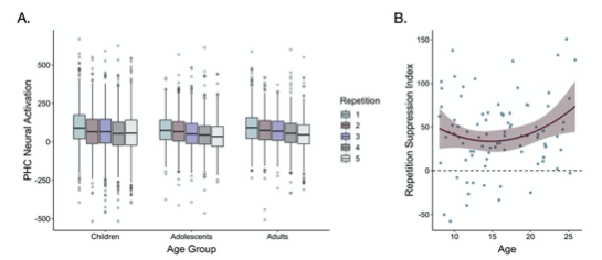
Fig 3. (A) Neural activation within a bilateral parahippocampal cortex ROI decreased across stimulus repetitions both linearly, F(1, 5015.9) = 30.64, p < .001, and quadratically, F(1, 9881.0) = 7.47, p = .006. Repetition suppression increased with linear age, F(1, 7267.5) = 7.2, p = .007, and quadratic age F(1, 7260.8) = 6.9, p = .009. The horizontal black lines indicate median neural activation values. The lower and upper edges of the boxes indicate the first and third quartiles of the grouped data, and the vertical lines extend to the smallest value no further than 1.5 times the interquartile range. Grey dots indicate data points outside those values. (B) The decrease in neural activation in the bilateral PHC ROI from the first to fifth repetition of each item also increased with both linear age, F(1, 78.32) = 3.97, p = .05, and quadratic age, F(1, 77.55) = 4.8, p = .031.
Second, the behavioral data show effects of age on both initial frequency learning and the effects of item frequency on memory. It is not clear whether the behavioral findings reflect the effects of age on the ability to use value information to prioritize memory or simply better initial learning of value-related information on older subjects.
Thank you for raising this important point. Indeed, one of our main findings is that older participants are better both at learning the structure of their environments and also at using structured knowledge to strategically prioritize memory. In our original manuscript, we described results of a model that included participants’ explicit frequency reports as a predictor of memory. Model comparison revealed that participants’ frequency reports — which we interpret as reflecting their beliefs about the structure of the environment — predicted memory more strongly than the item’s true frequency. In other words, participants’ beliefs about the structure of the environment (even if incorrect) more strongly influenced their memory encoding than the true structure of the environment. Critically, however, frequency reports interacted with age to predict memory (Fig 8). Even when we accounted for age-related differences in knowledge of the structure of the environment, older participants demonstrated a stronger influence of frequency on memory, suggesting they were better able to use their beliefs to control subsequent associative encoding. We have now clarified our interpretation of this model in our discussion on p. 23:
“Importantly, though we observed age-related differences in participants’ learning of the structure of their environment, the strengthening of the relation between frequency reports and associative memory with increasing age suggests that age differences in learning cannot fully account for age differences in value-guided memory. Even when accounting for individual differences in participants’ explicit knowledge of the structure of the environment, older participants demonstrated a stronger relation between their beliefs about item frequency and associative memory, suggesting that they used their beliefs to guide memory to a greater degree than younger participants.”
As noted by the reviewer, however, our initial memory analysis did not account for age-related differences in participants’ initial, online learning of item frequency, and our neural analyses further did not account for age differences in explicit frequency reports. We have now run additional control analyses to account for the potential influence of individual differences in frequency learning on associative memory. Specifically, for each participant, we computed three metrics: 1.) their overall accuracy during frequency-learning, 2.) their overall accuracy for the last presentation of each item during frequency-learning (as suggested by Reviewer 2), and 3.) the mean magnitude of the error in their frequency reports. We then included these metrics as covariates in our memory analyses.
When we include these control variables in our model, we continue to observe a robust effect of frequency condition (p < .001) as well as robust interactions between frequency condition and linear and quadratic age (ps < .003) on associative memory accuracy. We also observed a main effect of frequency error magnitude on memory accuracy (p < .001). Here, however, we no longer observe main effects of age or quadratic age on overall memory accuracy. Given the relation we observed between frequency error magnitudes and age, the results from this model suggests that there may be age-related improvements in overall memory that influence both memory for associations as well as learning of and memory for item frequencies. The fact that age no longer relates to overall memory when controlling for frequency error magnitudes suggest that age-related variance in memory for item frequencies and memory for associations are strongly related within individuals. Importantly, however, age-related variance in memory for item frequencies did not explain age-related variance in the influence of frequency condition on associative memory, suggesting that there are developmental differences in the use of knowledge of environmental structure to prioritize valuable information in memory that persist even when controlling for age-related differences in initial learning of environmental regularities. Given the importance of this analysis in elucidating the relation between the learning of environmental structure and value-guided memory, we have now updated the results in the main text of our manuscript to include them. Specifically, on p. 13, we now write:
“Because we observed age-related differences in participants’ online learning of item frequencies and in their explicit frequency reports, we further examined whether these age differences in initial learning could account for the age differences we observed in associative memory. To do so, we ran an additional model in which we included each participant’s mean frequency learning accuracy, mean frequency learning accuracy on the last repetition of each item, and explicit report error magnitude as covariates. Here, explicit report error magnitude predicted overall memory performance, χ2(1) =13.05, p < .001, and we did not observe main effects of age or quadratic age on memory performance (ps > .20). However, we continued to observe a main effect of frequency condition, χ2(1) = 19.65 p < .001, as well as significant interactions between frequency condition and both linear age χ2(1) = 10.59, p = .001, and quadratic age χ2(1) = 9.15, p = .002. Thus, while age differences in initial learning related to overall memory performance, they did not account for age differences in the use of environmental regularities to strategically prioritize memory for valuable information.”
In addition, as suggested by the reviewer, we also included the three covariates as control variables in our mediation analysis. When controlling for online frequency learning and explicit frequency report errors, PFC activity continued to mediate the relation between age and memory difference scores. We have now included these results on p. 16 - 17 of the main text:
“Further, when we included quadratic age, WASI scores, online frequency learning accuracy, online frequency learning accuracy on the final repetition of each item, and mean explicit frequency report error magnitudes as control variables in the mediation analysis, PFC activation continued to mediate the relation between linear age and memory difference scores (standardized indirect effect: .56, 95% confidence interval: [.06, 1.35], p = .023; standardized direct effect; 1.75, 95% confidence interval: [.12, .3.38], p = .034).”
We also refer to these analyses when we interpret our findings in our discussion. On p. 23, we write:
“In addition, we continued to observe a robust interaction between age and frequency condition on associative memory, even when controlling for age-related change in the accuracy of both online frequency learning and explicit frequency reports. Thus, though we observed age differences in the learning of environmental regularities and in their influence on subsequent associative memory encoding, our developmental memory effects cannot be fully explained by differences in initial learning.”
We thank the reviewer for this constructive suggestion, as we believe these control analyses strengthen our interpretation of age differences in both the learning and use of environmental regularities to prioritize memory.
Reviewer #2:
Nussenbaum and Hartley provide novel neurobehavioral evidence of how individuals differentially use incrementally acquired information to guide goal-relevant memory encoding, highlighting roles for the medial temporal lobe during frequency learning, and the lateral prefrontal cortex for value-guided encoding/retrieval. This provides a novel behavioral phenomenology that gives great insight into the processes guiding adaptive memory formation based on prior experience. However, there were a few weaknesses throughout the paper that undermined an overall mechanistic understanding of the processes.
First, there was a lack of anatomical specificity in the discussion and interpretation of both prefrontal and striatal targets, as there is great heterogeneity across these regions that would infer very different behavioral processes.
We agree with the reviewer that our introduction and discussion would benefit from more anatomical granularity, and we did indeed have a priori predictions about more specific neural regions that might be involved in our task.
First, we expected that both the ventral and dorsal striatum might be responsive to stimulus value across our age range. Prior work has suggested that activity in the ventral striatum often correlates with the intrinsic value of a stimulus, whereas activity in the dorsal striatum may reflect goal-directed action values (Liljeholm & O’Doherty, 2012). In our task, we expected that high-frequency items may acquire intrinsic value during frequency-learning that is then reflected in the striatal response to these items during encoding. However, because participants were not rewarded when they encountered these images, but rather incentivized to encode associations involving them, we hypothesized that the dorsal striatum may represent the value of the ‘action’ of remembering each pair. In line with this prediction, the dorsal striatum, and the caudate in particular, have also been shown to be engaged during value-guided cognitive control (Hikosaka et al., 2014; Insel et al., 2017).
We have now revised our introduction to include greater specificity in our anatomical predictions on p. 3:
“When individuals need to remember information associated with previously encountered stimuli (e.g., the grocery store aisle where an ingredient is located), frequency knowledge may be instantiated as value signals, engaging regions along the mesolimbic dopamine pathway that have been implicated in reward anticipation and the encoding of stimulus and action values. These areas include the ventral tegmental area (VTA) and the ventral and dorsal striatum (Adcock et al., 2006; Liljeholm & O’Doherty, 2012; Shigemune et al., 2014).”
Though we initially predicted that encoding of high-value information would be associated with increased activation in both the ventral and dorsal striatum, the activation we observed was largely within the dorsal striatum, and specifically, the caudate. We have now revised our discussion accordingly on p. 26:
“Though we initially hypothesized that both the ventral and dorsal striatum may be involved in encoding of high-value information, the activation we observed was largely within the dorsal striatum, a region that may reflect the value of goal-directed actions (Liljeholm & O’Doherty, 2012). In our task, rather than each stimulus acquiring intrinsic value during frequency-learning, participants may have represented the value of the ‘action’ of remembering each pair during encoding.”
Second, while the ventromedial PFC often reflects value, given the control demands of our task, we expected to see greater activity in the dorsolateral PFC, which is often engaged in tasks that require the implementation of cognitive control (Botvinick & Braver, 2015). Thus, we hypothesized that individuals would show increased activation in the dlPFC during encoding of high- vs. low-value information, and that this activation would vary as a function of age. We have now clarified this hypothesis on p. 3:
“Value responses in the striatum may signal the need for increased engagement of the dorsolateral prefrontal cortex (dlPFC) (Botvinick & Braver, 2015), which supports the implementation of strategic control.”
In our discussion, we review disparate findings in the developmental literature and discuss factors that may contribute to these differences across studies. For example, in our discussion of Davidow et al. (2016), we highlight differences between their task design and the present study, focusing on how their task involved immediate receipt of reward at the time of encoding, while our task incentivized memory accuracy. We further note that studies that involve reward delivery at the time of encoding may engage different neural pathways than those that promote goal-directed encoding. Beyond Davidow et al. (2016), there are no other neuroimaging studies that examine the influence of reward on memory across development. Thus, we cannot relate our present neural findings to prior work on the development of value-guided memory. As we note in our discussion (p. 28), “Further work is needed to characterize both the influence of different types of reward signals on memory across development, as well as the development of the neural pathways that underlie age-related change in behavior.”
Second, age-related differences in neural activation emerged both during the initial frequency learning as well as during memory-guided adaptive encoding. While data from this initial phase was used to unpack the behavioral relationships on adaptive memory, a major weakness of the paper was not connecting these measures to neural activity during memory encoding/retrieval. This would be especially relevant given that both implicit and explicit measures of frequency predicted subsequent performance, but it is unclear which of these measures was guiding lateral PFC and caudate responses.
Thank you for this valuable suggestion. We agree that it would be interesting to link frequency- learning behavior to neural activity at encoding. As such, we have now conducted additional analyses to explore these relations.
In the original version of our manuscript, we examined behavior at the item level through mixed- effects models, and neural activation during encoding at the participant level. Thus, to examine the relation between frequency-learning metrics and neural activation at encoding, we created two additional participant-level metrics. For each participant we computed their average repetition suppression index, and a measure of frequency distance. The average repetition suppression index reflects the overall extent to which the participant demonstrated repetition suppression in response to the fifth presentation of the high-frequency items, and is computed by averaging each participant’s repetition suppression indices across items. We hypothesized that participants who demonstrated the greatest degree of repetition suppression might be the most sensitive to the difference between the 1- and 5-frequency items, and therefore, show the greatest differences in striatal and PFC activation during encoding of high- vs. low-value information. The frequency distance metric reflects the average distance between participants’ explicit frequency reports for items that appeared once and items that appeared five times, and is computed by averaging their explicit frequency reports for items in each frequency condition, and then subtracting the average reports in the low-frequency condition from those in the high- frequency condition. We hypothesized that participants with the largest frequency distances might similarly be the most sensitive to the difference between the 1- and 5-frequency items, and therefore, show the greatest differences in striatal and PFC activation during encoding of high- vs. low-value information.
We first wanted to confirm that the relations we observed between repetition suppression, frequency reports, and age, could also be observed at the participant level. In line with our prior, behavioral analyses, we found that age related to both mean repetition suppression indices (marginally; linear age: p = .067; quadratic age: p = .042); and frequency distances (linear and quadratic age: ps < .001).
In addition, we further tested whether these two metrics related to memory performance. In contrast to our item-level findings, we did not observe a significant relation between repetition suppression indices and memory (p = .83). We did observe an effect of frequency distance on memory performance. Specifically, we observed significant interactions between frequency distance and age (p = .014) and frequency distance and quadratic age (p = .021) on memory difference scores, such that the influence of frequency distance on memory difference scores increased with increasing age from childhood to adolescence.
We next examined how mean repetition suppression indices and frequency distances related to differential neural activation during encoding of high- and low-value pairs. In line with our memory findings, we did not observe any significant relations between mean repetition suppression indices and neural activation in the caudate or prefrontal cortex during encoding (ps > .15).
Frequency distance did not relate to caudate activation during encoding nor did we observe a frequency distance x age interaction effect (ps > .16). Frequency distance did, however, relate to differential PFC activation during encoding of high- vs. low-value pairs. Specifically, we observed a main effect of frequency distance on PFC activation (p = .0012), such that participants whose explicit reports of item frequency, were on average, more distinct across frequency conditions, demonstrated increased PFC activation during encoding of pairs involving high- vs. low-frequency items. Interestingly, when we included frequency distance in our model, we no longer observed a significant effect of age on differential PFC activation, nor did we observe a significant frequency distance x age interaction (ps > .13). These findings suggest that PFC activation during encoding may have, in part, reflected participants’ beliefs about the structure of the environment, with participants demonstrating stronger differential engagement of control processes across conditions when their representations of the conditions themselves were more distinct.
Finally, we examined how age, frequency distance, and PFC activation related to memory difference scores. Here, even when controlling for both frequency distance and PFC activation, we continued to observe main effects of age and quadratic age on memory difference scores (linear age: p = .006; quadratic age: p = .001). In line with our analysis of the relation between frequency reports and memory, these results suggest that age-related variance in value-guided memory may depend on both knowledge of the structure of the environment and use of that knowledge to effectively control encoding.
We have now added these results to our manuscript on p. 13 - 14. We write:
“Given the relations we observed between memory and both repetition suppression and frequency reports, we examined whether they related to neural activation in both our caudate and PFC ROI during encoding. To do so, we computed each participant’s average repetition suppression index, and their “frequency distance” — or the average difference in their explicit reports for items in the high- and low-frequency conditions. We expected that participants with greater average repetition suppression indices and greater frequency distances represented the high- and low-frequency items as more distinct from one another and therefore would show greater differences in neural activation at encoding across frequency conditions. In line with our prior analyses, both metrics varied with age (though repetition suppression only marginally (linear age: p = .067; quadratic age: p = .042); Appendix 3 y Tables 22 and 25), suggesting that older participants demonstrated better learning of the structure of the environment. We ran linear regressions examining the relations between each metric, age, and their interaction on neural activation in both the caudate and PFC. We observed no significant effects or interactions of average repetition suppression indices on neural activation (ps > .15; Appendix 3 Tables 23 and 24). We did, however, observe a significant effect of frequency distance on PFC activation (β = .42, SE = .12, p = .0012), such that participants who believed that average frequencies of the high- and low-frequency items were further apart also demonstrated greater PFC activation during encoding of pairs with high- vs. low-frequency items. Here, we did not observe a significant effect of age on PFC activation (β = -.03, SE = .13, p = .82), suggesting that age-related variance in PFC activation may be related to age differences in explicit frequency beliefs. Importantly, however, even when we accounted for both PFC activation and frequency distances, we continued to observe an effect of age on memory difference scores (β = .56, SE = .20, p = .006), which, together with our prior analyses, suggest that developmental differences in value-guided memory are not driven solely by age differences in beliefs about the structure of the environment but also depend on the use of those beliefs to guide encoding.”
We have added the full model results to Appendix 3: Full Model Specification and Results.
Given these results, we have now revised our interpretation of our neural data. Our memory analyses demonstrate that across our age range, we observed age-related differences in both the acquisition of knowledge of the structure of the environment and in its use. Originally, we interpreted the PFC activation as reflecting the use of learned value to guide memory. However, the strong relation we found between frequency distance and PFC activation suggests that the age differences in PFC activation that we observed may also be related to age differences in knowledge of the structure of the environment that governs when control processes should be engaged most strongly. However, these results must be interpreted cautiously. Participants provided explicit frequency reports after they completed the encoding and retrieval tasks, and so explicit frequency reports may have been influenced not only by participants’ memories of online frequency learning, but also by the strength with which they encoded the item and its paired associate, and the experience of successfully retrieving it.
We have now revised our discussion to consider these results. On p. 23, we now write,
“Our neural results further suggest that developmental differences in memory were driven by both knowledge of the structure of the environment and use of that knowledge to guide encoding.”
On p. 24, we write,
“The development of adaptive memory requires not only the implementation of encoding and retrieval strategies, but also the flexibility to up- or down-regulate the engagement of control in response to momentary fluctuations in information value (Castel et al., 2007, 2013; Hennessee et al., 2017). Importantly, value-based modulation of lateral PFC engagement during encoding mediated the relation between age and memory selectivity, suggesting that developmental change in both the representation of learned value and value-guided cognitive control may underpin the emergence of adaptive memory prioritization. Prior work examining other neurocognitive processes, including response inhibition (Insel et al., 2017) and selective attention (Störmer et al., 2014), has similarly found that increases in the flexible upregulation of control in response to value cues enhance goal-directed behavior across development (Davidow et al., 2018), and may depend on the engagement of both striatal and prefrontal circuitry (Hallquist et al., 2018; Insel et al., 2017). Here, we extend these past findings to the domain of memory, demonstrating that value signals derived from the structure of the environment increasingly elicit prefrontal cortex engagement and strengthen goal-directed encoding across childhood and into adolescence.”
And on p. 25, we have added an additional paragraph:
“Further, we also demonstrate that in the absence of explicit value cues, the engagement of prefrontal control processes may reflect beliefs about information value that are learned through experience. Here, we found that differential PFC activation during encoding of high- vs. low-value information reflected individual and age-related differences in beliefs about the structure of the environment; participants who represented the average frequencies of the low- and high-frequency items as further apart also demonstrated greater value-based modulation of lateral PFC activation. It is important to note, however, that we collected explicit frequency reports after associative encoding and retrieval. Thus the relation between PFC activation and explicit frequency reports may be bidirectional — while participants may have increased the recruitment of cognitive control processes to better encode information they believed was more valuable, the engagement of more elaborative or deeper encoding strategies that led to stronger memory traces may have also increased participants’ subjective sense of an item’s frequency (Jonides & Naveh-Benjamin, 1987).”
Third, more discussion is warranted on the nature of age-related changes given that some findings followed quadratic functions and others showed linear. Further interpretation of the quadratic versus linear fits would provide greater insight into the relative rates of maturation across discrete neurobehavioral processes.
We agree with the reviewer that more discussion is warranted here. While many cognitive processes tend to improve with increasing age, the significant interaction between quadratic age and frequency condition on memory accuracy could reflect a number of different patterns of developmental variance. Because quadratic curves are U-shaped, the significant interaction between quadratic age and frequency condition could reflect a peak in value-guided memory in adolescence. However, the combination of linear and quadratic effects can also capture “plateauing” effects, where the influence of age on a particular cognitive process decreases at a particular developmental timepoint. To determine how to interpret the quadratic effect of age on value-guided memory — and specifically, to test for the presence of an adolescent peak — we ran an additional analysis.
To test for an adolescent peak in value-guided memory, we first fit our memory accuracy model without any age terms, and then extracted the random slope across frequency conditions for each subject. We then conducted a ‘two lines test’ (Simonsohn, 2018) to examine the relation between age and these random slopes. In brief, the two-lines test fits the data with two linear models — one with a positive slope and one with a negative slope, algorithmically determining the breakpoint in the estimates where the signs of the slopes change. When we analyzed our memory data in this way, we found a robust, positive relation between age and value-guided memory (see newly added Appendix 2 Figure 3, also below) from childhood to mid- adolescence, that peaked around age 16 (age 15.86). From age ~16 to early adulthood, however, we observed only a marginal negative relation between age and value-guided memory (p = .0567). Thus, our findings do not offer strong evidence in support of an adolescent peak in value-guided memory — instead, they suggest that improvements in value-guided memory are strongest from childhood to adolescence.
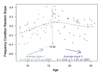
Appendix 2 - Figure 3. Results from the two-lines test (Simonsohn, 2018) revealed that the influence of frequency condition on memory accuracy increased throughout childhood and early adolescence, and did not significantly decrease from adolescence into early adulthood.
To more clearly demonstrate the relation between age and value-guided memory, we have now included the results of the two-lines test in the results section of our main text. On p. 12 - 13, we write:
“In line with our hypothesis, we observed a main effect of frequency condition on memory, χ2(1) = 21.51, p <.001, indicating that individuals used naturalistic value signals to prioritize memory for high-value information. Critically, this effect interacted with both linear age (χ2(1) = 11.03, p < .001) and quadratic age (χ2(1) = 9.51, p = .002), such that the influence of frequency condition on memory increased to the greatest extent throughout childhood and early adolescence. To determine whether the interaction between quadratic age and frequency condition on memory accuracy reflected an adolescent peak in value-guided memory prioritization, we re-ran our memory accuracy model without including any age terms, and extracted each participant’s random slope across frequency conditions. We then submitted these random slopes to the “two-lines” test (Simonsohn, 2018), which fits two regression lines with oppositely signed slopes to the data, algorithmically determining where the sign flip should occur. The results of this analysis revealed that the influence of frequency condition on memory significantly increased from age 8 to age 15.86 (b = .03, z = 2.71, p = .0068; Appendix 2 – Figure 3), but only marginally decreased from age 15.86 to age 25 (b = -.02, z = 1.91, p = .0576). Thus, the interaction between frequency condition and quadratic age on memory performance suggests that the biggest age differences in value-guided memory occurred through childhood and early adolescence, with older adolescents and adults performing similarly.”
That said, this developmental trajectory is likely specific to the particular demands of our task. In our previous behavioral study that used a very similar paradigm (Nussenbaum, Prentis, & Hartley, 2018), we observed only a linear relation between age and value-guided memory.
Although the task used in our behavioral study was largely similar to the task we employed here, there were subtle differences in the design that may have extended the age range through which we observed improvements in memory prioritization. In particular, in our previous behavioral study, the memory test required participants to select the correct associate from a grid of 20 options (i.e., 1 correct and 19 incorrect options), whereas here, participants had to select the correct associate from a grid of 4 options (1 correct and 3 incorrect options). In our prior work, the need to differentiate the ‘correct’ option from many more foils may have increased the demands on either (or both) memory encoding or memory retrieval, requiring participants to encode and retrieve more specific representations that would be less confusable with other memory representations. By decreasing the task demands in the present study, we may have shifted the developmental curve we observed toward earlier developmental timepoints.
We originally did not emphasize our quadratic findings in the discussion of our manuscript because, given the marginal decrease in memory selectivity we observed from age 16 to age 25 and the different age-related findings across our two studies, we did not want to make strong claims about the specific shape of developmental change. However, we agree with the reviewer that these points are worthy of discussion within the manuscript. We have now amended our discussion on p. 25 accordingly:
“We found that memory prioritization varied with quadratic age, and our follow-up tests probing the quadratic age effect did not reveal evidence for significant age-related change in memory prioritization between late adolescence and early adulthood. However, in our prior behavioral work using a very similar paradigm (Nussenbaum et al., 2020), we found that memory prioritization varied with linear age only. In line with theoretical proposals (Davidow et al., 2018), subtle differences in the control demands between the two tasks (e.g., reducing the number of ‘foils’ presented on each trial of the memory test here relative to our prior study), may have shifted the age range across which we observed differences in behavior, with the more demanding variant of our task showing more linear age-related improvements into early adulthood. In addition, the specific control demands of our task may have also influenced the age at which value- guided memory emerged. Future studies should test whether younger children can modulate encoding based on the value of information if the mnemonic demands of the task are simpler.”
We thank the reviewer for this helpful suggestion, and believe our additions that expand on the quadratic age effects help clarify our developmental findings.
Although hippocamapal and PHC results did not show a main effect of value, it seems by the introduction that this region would be critical for the processes under study. I would suggest including these regions as ROIs of interest guiding age-related differences during the memory encoding and retrieval phases. Even reporting negative findings for these regions would be helpful to readers, especially given the speculation of the negative findings in the discussion.
Thank you for this suggestion. We have now examined how differential neural activation within the hippocampus and parahippocampal cortex during encoding of high- vs. low-value information varies with age. To do so, we followed the same approach as with our PFC and caudate ROI analyses. Specifically, we first identified the voxel within both the hippocampus and parahippocampal cortex with the highest z-statistic from our group-level 5 > 1 encoding contrast. We then drew a 5-mm sphere around these voxels and examined how mean beta weights within these spheres varied with age.
We did not observe any relation between differential hippocampal or parahippocampal cortex activation during encoding of high- vs. low-value information and age (ps > .50). We agree with the reviewer that these results are informative, and have now added them to Appendix 2: Supplementary Analyses, which we refer to in the main text (p. 15). In Appendix 2, we write:
“Hippocampal and parahippocampal cortex activation during encoding A priori, we expected that regions in the medial temporal lobe that have been linked to successful memory formation, including the hippocampus and parahippocampal cortex (Davachi, 2006), may be differentially engaged during encoding of high- vs. low- value information. Further, we hypothesized that the differential engagement of these regions across age may contribute to age differences in value-guided memory. Though we did not see any significant clusters of activation in the hippocampus or parahippocampal cortex in our group level high value vs. low value encoding contrast, we conducted additional ROI analyses to test these hypotheses. As with our other ROI analyses, we first identified the peak voxel (based on its z-statistic; hippocampus: x = 24, y = 34, z = 23; parahippocampal cortex: x = 22, y = 41, z = 16) in each region from our group-level contrast, and then drew 5-mm spheres around them. We then examined how average parameter estimates within these spheres related to both age and memory difference scores.
First, we ran a linear regression modeling the effects of age, WASI scores, and their interaction on hippocampal activation. We did not observe a main effect of age on hippocampal activation, (β = .00, SE = .10, p > .99). We did, however, observe a significant age x WASI score interaction effect (β = .30, SE = .10, p = .003). Next, we conducted another linear regression to examine the effects of hippocampal activation, age, WASI scores, and their interaction on memory difference scores. In contrast to our prefrontal cortex activation results, activation in the hippocampus did not relate to memory difference scores, (β = -.02, SE = .03, p = .50).
We repeated these analyses with our parahippocampal cortex sphere. Here, we did not observe any significant effects of age on parahippocampal activation (β = -.07, SE = .11, p = .50), nor did we observe any effects of parahippocampal activation on memory difference scores (β = .01, SE = .03, p = .25).”
Reviewer #3:
This paper investigated age differences in the neurocognitive mechanisms of value-based memory encoding and retrieval across children, adolescents and young adults. It used a novel experimental paradigm in combination with fMRI to disentangle age differences in determining the value of information based on its frequency from the usage of these learned value signals to guide memory encoding. During value learning, younger participants demonstrated a stronger effect of item repetition on response accuracy, whereas repetition suppression effects in a parahippocampal ROI were strongest in adults. Item frequency modulated memory accuracy such that associative memory was better for previously high-frequency value items. Notably, this effect increased with age. Differences in memory accuracy between low- and high-frequency items were associated with left lateral PFC activation which also increased with age. Accordingly, a mediation analyses revealed that PFC activation mediated the relation between age and memory benefit for high- vs. low-frequency items. Finally, both participants' representations of item frequency (which were more likely to deviate in younger children) and repetition suppression in the parahippocampal ROI were associated with higher memory accuracy. Together, these results data add to the still scarce literature examining how information value influences memory processes across development.
Overall, the conclusions of the paper are well supported by the data, but some aspects of the data analysis need to be clarified and extended.
Empirical findings directly comparing cross-sectional and longitudinal effects have demonstrated that cross-sectional analyses of age differences do not readily generalize to longitudinal research (e.g., Raz et al., 2005; Raz & Lindenberger, 2012). Formal analyses have demonstrated that proportion of explained age-related variance in cross-sectional mediation models may stem from various factors, including similar mean age trends, within-time correlations between a mediator and an outcome, or both (Lindenberger et al., 2011; see also Hofer, Flaherty, & Hoffman, 2006; Maxwell & Cole, 2007). Thus, the results of the mediation analysis showing that PFC activation explains age-related variance in memory difference scores, cannot be taken to imply that changes in PFC activation are correlated with changes in value-guided memory. While the general limitations of a cross-sectional study are noted in the Discussion of the manuscript, it would be important to discuss the critical limitations of the mediation analysis. While the main conclusions of the paper do not critically depend on this analysis, it would be important to alert the reader to the limited information value in performing cross-sectional mediation analyses of age variance.
Thank you for raising this critical point. We have expanded our discussion to specifically note the limitations of our mediation analysis and to more strongly emphasize the need for future longitudinal studies to reveal how changes in neural circuitry may support the emergence of motivated memory across development. Specifically, on p. 26, we now write:
“One important caveat is that our study was cross-sectional — it will be important to replicate our findings in a longitudinal sample to more directly measure how developmental changes in cognitive control within an individual contribute to changes in their ability to selectively encode useful information. Our mediation results, in particular, must be interpreted with caution as simulations have demonstrated that in cross-sectional samples, variables can emerge as significant mediators of age-related change due largely to statistical artifact (Hofer, Flaherty, & Hoffman, 2006; Lindenberger et al., 2011). Indeed, our finding that PFC activation mediates the relation between age and value-guided memory does not necessarily imply that within an individual, PFC development leads to improvements in memory selectivity. Longitudinal work in which individuals’ neural activity and memory performance is sampled densely within developmental windows of interest is needed to elucidate the complex relations between age, brain development, and behavior (Hofer, Flaherty, & Hoffman, 2006; Lindenberger et al., 2011).”
It would be helpful to provide more information on how chance memory performance was handled during data analysis, especially as it is more likely to occur in younger participants. Related to this, please connect the points that belong to the same individual in Figure 3 to facilitate evaluation of individual differences in the memory difference scores.
Thank you for raising this important point. On each memory test trial, participants viewed the item (either a postcard or picture) above images of four possible paired associates (see Figure 1 on p. 6). On each memory test trial, participants had 6 seconds to select one of these items. If participants did not make a response within 6 seconds, that trial was considered ‘missed.’ Missed trials were excluded from behavioral analyses and regressed out in neural analyses. If participants selected the correct associate, memory accuracy was coded as ‘1;’ if they selected an incorrect associate, accuracy was coded as ‘0.’ On each trial, there was 1 correct option and 3 incorrect options. As such, chance-level memory performance was 25%. We have now clarified this on p. 34 and included a dashed line indicating chance-level performance within Fig. 4 (formerly Figure 3) on p. 12. In addition, we have also updated Figure 4 (see below) to connect the points belonging to the same participants, as suggested by the reviewer.
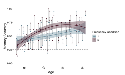
Figure 4. Participants demonstrated prioritization of memory for high-value information, as indicated by higher memory accuracy for associations involving items in the five- relative to the one-frequency condition (χ2(1) = 19.73, p <.001). The effects of item frequency on associative memory increased throughout childhood and into adolescence (linear age x frequency condition: χ2(1) = 10.74, p = .001; quadratic age x frequency condition: χ2(1) = 9.27, p = .002).
Out of 90 participants, 2 children performed at or below chance (<= 25% memory accuracy). Interpreting the behavior of the participants who responded to fewer than 12 out of 48 trials correctly is challenging. On the one hand, they might not have remembered anything and responded correctly on these trials due to randomly guessing. On the other hand, they may have implemented an encoding strategy of focusing only on a small number of pairs. Thus, a priori, based on the analysis approach we implemented in our prior, behavioral study (Nussenbaum et al., 2019), we decided to include all participants in our memory analyses, regardless of their overall accuracy. However, when we exclude these two participants from our memory analyses, our main findings still hold. Specifically, we continue to observe main effects of frequency condition and age, and interactions between frequency condition and both linear and quadratic age on associative memory accuracy (ps < .012).
We have now clarified these details about chance-level performance in the methods section of our manuscript on p. 34.
“For our memory analyses, trials were scored as ‘correct’ if the participant selected the correct association from the set of four possible options presented during the memory test, ‘incorrect’ if the participant selected an incorrect association, and ‘missed’ if the participant failed to respond within the 6-second response window. Missed trials were excluded from all analyses. Because participants had to select the correct association from four possible options, chance-level performance was 25%. Two child participants performed at or below chance-level on the memory test. They were included in all analyses reported in the manuscript; however, we report full details of the results of our memory analyses when we exclude these two participants in Appendix 3 (Table 15). Importantly, our main findings remain unchanged.”
In Appendix 3, we include a table with the full results from our memory model without these two participants:
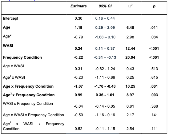
Appendix Table 15: Associative memory accuracy by frequency condition (below chance subjects excluded)
I would like to see some consideration of how the different signatures of value learning, repetition suppression and reported item frequency, are related to the observed PFC and caudate effects during memory encoding. Such a discussion would help the reader connect the findings on learning and using information value across development.
Thank you for this valuable suggestion. We agree that it would be interesting to link frequency- learning behavior to neural activity at encoding. As such, we have now conducted additional analyses to explore these relations.
In the original version of our manuscript, we examined behavior at the item level through mixed- effects models, and neural activation during encoding at the participant level. Thus, to examine the relation between frequency-learning metrics and neural activation at encoding, we created two additional participant-level metrics. For each participant we computed their average repetition suppression index, and a measure of frequency distance. The average repetition suppression index reflects the overall extent to which the participant demonstrated repetition suppression in response to the fifth presentation of the high-frequency items, and is computed by averaging each participant’s repetition suppression indices across items. We hypothesized that participants who demonstrated the greatest degree of repetition suppression might be the most sensitive to the difference between the 1- and 5-frequency items, and therefore, show the greatest differences in striatal and PFC activation during encoding of high- vs. low-value information. The frequency distance metric reflects the average distance between participants’ explicit frequency reports for items that appeared once and items that appeared five times, and is computed by averaging their explicit frequency reports for items in each frequency condition, and then subtracting the average reports in the low-frequency condition from those in the high- frequency condition. We hypothesized that participants with the largest frequency distances might similarly be the most sensitive to the difference between the 1- and 5-frequency items, and therefore, show the greatest differences in striatal and PFC activation during encoding of high- vs. low-value information.
We first wanted to confirm that the relations we observed between repetition suppression, frequency reports, and age, could also be observed at the participant level. In line with our prior, behavioral analyses, we found that age related to both mean repetition suppression indices (marginally; linear age: p = .067; quadratic age: p = .042); and frequency distances (linear and quadratic age: ps < .001).
In addition, we further tested whether these two metrics related to memory performance. In contrast to our item-level findings, we did not observe a significant relation between repetition suppression indices and memory (p = .83). We did observe an effect of frequency distance on memory performance. Specifically, we observed significant interactions between frequency distance and age (p = .014) and frequency distance and quadratic age (p = .021) on memory difference scores, such that the influence of frequency distance on memory difference scores increased with increasing age from childhood to adolescence.
We next examined how mean repetition suppression indices and frequency distances related to differential neural activation during encoding of high- and low-value pairs. In line with our memory findings, we did not observe any significant relations between mean repetition suppression indices and neural activation in the caudate or prefrontal cortex during encoding (ps > .15).
Frequency distance did not relate to caudate activation during encoding nor did we observe a frequency distance x age interaction effect (ps > .16). Frequency distance did, however, relate to differential PFC activation during encoding of high- vs. low-value pairs. Specifically, we observed a main effect of frequency distance on PFC activation (p = .0012), such that participants whose explicit reports of item frequency, were on average, more distinct across frequency conditions, demonstrated increased PFC activation during encoding of pairs involving high- vs. low-frequency items. Interestingly, when we included frequency distance in our model, we no longer observed a significant effect of age on differential PFC activation, nor did we observe a significant frequency distance x age interaction (ps > .13). These findings suggest that PFC activation during encoding may have, in part, reflected participants’ beliefs about the structure of the environment, with participants demonstrating stronger differential engagement of control processes across conditions when their representations of the conditions themselves were more distinct.
Finally, we examined how age, frequency distance, and PFC activation related to memory difference scores. Here, even when controlling for both frequency distance and PFC activation, we continued to observe main effects of age and quadratic age on memory difference scores (linear age: p = .006; quadratic age: p = .001). In line with our analysis of the relation between frequency reports and memory, these results suggest that age-related variance in value-guided memory may depend on both knowledge of the structure of the environment and use of that knowledge to effectively control encoding.
We have now added these results to our manuscript on p. 13 - 14. We write:
“Given the relations we observed between memory and both repetition suppression and frequency reports, we examined whether they related to neural activation in both our caudate and PFC ROI during encoding. To do so, we computed each participant’s average repetition suppression index, and their “frequency distance” — or the average difference in their explicit reports for items in the high- and low-frequency conditions. We expected that participants with greater average repetition suppression indices and greater frequency distances represented the high- and low-frequency items as more distinct from one another and therefore would show greater differences in neural activation at encoding across frequency conditions. In line with our prior analyses, both metrics varied with age (though repetition suppression only marginally (linear age: p = .067; quadratic age: p = .042); Appendix 3 Tables 22 and 25), suggesting that older participants demonstrated better learning of the structure of the environment. We ran linear regressions examining the relations between each metric, age, and their interaction on neural activation in both the caudate and PFC. We observed no significant effects or interactions of average repetition suppression indices on neural activation (ps > .15; Appendix 3 Tables 23 and 24). We did, however, observe a significant effect of frequency distance on PFC activation (β = .42, SE = .12, p = .0012), such that participants who believed that average frequencies of the high- and low-frequency items were further apart also demonstrated greater PFC activation during encoding of pairs with high- vs. low-frequency items. Here, we did not observe a significant effect of age on PFC activation (β = -.03, SE = .13, p = .82), suggesting that age-related variance in PFC activation may be related to age differences in explicit frequency beliefs. Importantly, however, even when we accounted for both PFC activation and frequency distances, we continued to observe an effect of age on memory difference scores (β = .56, SE = .20, p = .006), which, together with our prior analyses, suggest that developmental differences in value-guided memory are not driven solely by age differences in beliefs about the structure of the environment but also depend on the use of those beliefs to guide encoding.”
We have added the full model results to Appendix 3.
Given these results, we have now revised our interpretation of our neural data. Our memory analyses demonstrate that across our age range, we observed age-related differences in both the acquisition of knowledge of the structure of the environment and in its use. Originally, we interpreted the PFC activation as reflecting the use of learned value to guide memory. However, the strong relation we found between frequency distance and PFC activation suggests that the age differences in PFC activation that we observed may also be related to age differences in knowledge of the structure of the environment that governs when control processes should be engaged most strongly. However, these results must be interpreted cautiously. Participants provided explicit frequency reports after they completed the encoding and retrieval tasks, and so explicit frequency reports may have been influenced not only by participants’ memories of online frequency learning, but also by the strength with which they encoded the item and its paired associate, and the experience of successfully retrieving it.
We have now revised our discussion to consider these results. On p. 23, we now write,
“Our neural results further suggest that developmental differences in memory were driven by both knowledge of the structure of the environment and use of that knowledge to guide encoding.”
n p. 24, we write,
“The development of adaptive memory requires not only the implementation of encoding and retrieval strategies, but also the flexibility to up- or down-regulate the engagement of control in response to momentary fluctuations in information value (Castel et al., 2007, 2013; Hennessee et al., 2017). Importantly, value-based modulation of lateral PFC engagement during encoding mediated the relation between age and memory selectivity, suggesting that developmental change in both the representation of learned value and value-guided cognitive control may underpin the emergence of adaptive memory prioritization. Prior work examining other neurocognitive processes, including response inhibition (Insel et al., 2017) and selective attention (Störmer et al., 2014), has similarly found that increases in the flexible upregulation of control in response to value cues enhance goal-directed behavior across development (Davidow et al., 2018), and may depend on the engagement of both striatal and prefrontal circuitry (Hallquist et al., 2018; Insel et al., 2017). Here, we extend these past findings to the domain of memory, demonstrating that value signals derived from the structure of the environment increasingly elicit prefrontal cortex engagement and strengthen goal-directed encoding across childhood and into adolescence.”
And on p. 25, we have added an additional paragraph:
“Further, we also demonstrate that in the absence of explicit value cues, the engagement of prefrontal control processes may reflect beliefs about information value that are learned through experience. Here, we found that differential PFC activation during encoding of high- vs. low-value information reflected individual and age-related differences in beliefs about the structure of the environment; participants who represented the average frequencies of the low- and high-frequency items as further apart also demonstrated greater value-based modulation of lateral PFC activation. It is important to note, however, that we collected explicit frequency reports after associative encoding and retrieval. Thus the relation between PFC activation and explicit frequency reports may be bidirectional — while participants may have increased the recruitment of cognitive control processes to better encode information they believed was more valuable, the engagement of more elaborative or deeper encoding strategies that led to stronger memory traces may have also increased participants’ subjective sense of an item’s frequency (Jonides & Naveh-Benjamin, 1987).”
A point worthy of discussion are the implications of the finding that younger participants demonstrated greater deviations in their frequency reports for the development of value learning, given that frequency reports were found to predict associative memory accuracy.
Thank you for raising this important point. Indeed, one of our main findings is that older participants are better both at learning the structure of their environments and also at using structured knowledge to strategically prioritize memory. In our original manuscript, we described results of a model that included participants’ explicit frequency reports as a predictor of memory. Model comparison revealed that participants’ frequency reports — which we interpret as reflecting their beliefs about the structure of the environment — predicted memory more strongly than the item’s true frequency. In other words, participants’ beliefs about the structure of the environment (even if incorrect) more strongly influenced their memory encoding than the true structure of the environment. Critically, however, frequency reports interacted with age to predict memory (Fig 8). Even when we accounted for age-related differences in knowledge of the structure of the environment, older participants demonstrated a stronger influence of frequency on memory, suggesting they were better able to use their beliefs to control subsequent associative encoding. We have now clarified our interpretation of this model in our discussion on p. 23:
“Importantly, though we observed age-related differences in participants’ learning of the structure of their environment, the strengthening of the relation between frequency reports and associative memory with increasing age suggests that age differences in learning cannot fully account for age differences in value-guided memory. Even when accounting for individual differences in participants’ explicit knowledge of the structure of the environment, older participants demonstrated a stronger relation between their beliefs about item frequency and associative memory, suggesting that they used their beliefs to guide memory to a greater degree than younger participants.”
As noted by the reviewer, however, our initial memory analysis did not account for age-related differences in participants’ initial, online learning of item frequency, and our neural analyses further did not account for age differences in explicit frequency reports. We have now run additional control analyses to account for the potential influence of individual differences in frequency learning on associative memory. Specifically, for each participant, we computed three metrics: 1.) their overall accuracy during frequency-learning, 2.) their overall accuracy for the last presentation of each item during frequency-learning (as suggested by Reviewer 2), and 3.) the mean magnitude of the error in their frequency reports. We then included these metrics as covariates in our memory analyses.
When we include these control variables in our model, we continue to observe a robust effect of frequency condition (p < .001) as well as robust interactions between frequency condition and linear and quadratic age (ps < .003) on associative memory accuracy. We also observed a main effect of frequency error magnitude on memory accuracy (p < .001). Here, however, we no longer observe main effects of age or quadratic age on overall memory accuracy. Given the relation we observed between frequency error magnitudes and age, the results from this model suggests that there may be age-related improvements in overall memory that influence both memory for associations as well as learning of and memory for item frequencies. The fact that age no longer relates to overall memory when controlling for frequency error magnitudes suggest that age-related variance in memory for item frequencies and memory for associations are strongly related within individuals. Importantly, however, age-related variance in memory for item frequencies did not explain age-related variance in the influence of frequency condition on associative memory, suggesting that there are developmental differences in the use of knowledge of environmental structure to prioritize valuable information in memory that persist even when controlling for age-related differences in initial learning of environmental regularities. Given the importance of this analysis in elucidating the relation between the learning of environmental structure and value-guided memory, we have now updated the results in the main text of our manuscript to include them. Specifically, on p. 13, we now write:
“Because we observed age-related differences in participants’ online learning of item frequencies and in their explicit frequency reports, we further examined whether these age differences in initial learning could account for the age differences we observed in associative memory. To do so, we ran an additional model in which we included each participant’s mean frequency learning accuracy, mean frequency learning accuracy on the last repetition of each item, and explicit report error magnitude as covariates. Here, explicit report error magnitude predicted overall memory performance, χ2(1) =13.05, p < .001, and we did not observe main effects of age or quadratic age on memory performance (ps > .20). However, we continued to observe a main effect of frequency condition, χ2(1) = 19.65 p < .001, as well as significant interactions between frequency condition and both linear age χ2(1) = 10.59, p = .001, and quadratic age χ2(1) = 9.15, p = .002. Thus, while age differences in initial learning related to overall memory performance, they did not account for age differences in the use of environmental regularities to strategically prioritize memory for valuable information.”
In addition, as suggested by the reviewer, we also included the three covariates as control variables in our mediation analysis. When controlling for online frequency learning and explicit frequency report errors, PFC activity continued to mediate the relation between age and memory difference scores. We have now included these results on p. 16 - 17 of the main text:
“Further, when we included quadratic age, WASI scores, online frequency learning accuracy, online frequency learning accuracy on the final repetition of each item, and mean explicit frequency report error magnitudes as control variables in the mediation analysis, PFC activation continued to mediate the relation between linear age and memory difference scores (standardized indirect effect: .56, 95% confidence interval: [.06, 1.35], p = .023; standardized direct effect; 1.75, 95% confidence interval: [.12, .3.38], p = .034).”
We also refer to these analyses when we interpret our findings in our discussion. On p. 23, we write:
“In addition, we continued to observe a robust interaction between age and frequency condition on associative memory, even when controlling for age-related change in the accuracy of both online frequency learning and explicit frequency reports. Thus, though we observed age differences in the learning of environmental regularities and in their influence on subsequent associative memory encoding, our developmental memory effects cannot be fully explained by differences in initial learning.”
We thank the reviewer for this constructive suggestion, as we believe these control analyses strengthen our interpretation of age differences in both the learning and use of environmental regularities to prioritize memory.
Author response:
The following is the authors’ response to the previous reviews.
Reviewer #1 (Public review):
Summary:
This work shows that a specific adenosine deaminase protein in Dictyostelium generates the ammonia that is required for tip formation during Dictyostelium development. Cells with an insertion in the ADGF gene aggregate but do not form tips. A remarkable result, shown in several different ways, is that the ADGF mutant can be rescued by exposing the mutant to ammonia gas. The authors also describe other phenotypes of the ADGF mutant such as increased mound size, altered cAMP signalling, and abnormal cell type differentiation. It appears that the ADGF mutant has defects in the expression of a large number of genes, resulting in not only the tip defect but also the mound size, cAMP signalling, and differentiation phenotypes.
Strengths:
The data and statistics are excellent.
(1) Weaknesses: The key weakness is understanding why the cells bother to use a diffusible gas like ammonia as a signal to form a tip and continue development.
Ammonia can come from a variety of sources both within and outside the cells and this can be from dead cells also. Ammonia by increasing cAMP levels, trigger collective cell movement thereby establishing a tip in Dictyostelium. A gaseous signal can act over long distances in a short time and for instance ammonia promotes synchronous development in a colony of yeast cells (Palkova et al., 1997; Palkova and Forstova, 2000). The slug tip is known to release ammonia probably favouring synchronized development of the entire colony of Dictyostelium. However, after the tips are established ammonia exerts negative chemotaxis probably helping the slugs to move away from each other ensuring equal spacing of the fruiting bodies (Feit and Sollitto, 1987).
It is well known that ammonia serves as a signalling molecule influencing both multicellular organization and differentiation in Dictyostelium (Francis, 1964; Bonner et al., 1989; Bradbury and Gross, 1989). Ammonia by raising the pH of the intracellular acidic vesicles of prestalk cells (Poole and Ohkuma, 1981; Gross et al, 1983), and the cytoplasm, is known to increase the speed of chemotaxing amoebae (Siegert and Weijer, 1989; Van Duijn and Inouye, 1991), inducing collective cell movement (Bonner et al., 1988, 1989), favoring tipped mound development.
Ammonia produced in millimolar concentrations during tip formation (Schindler and Sussman, 1977) could ward off other predators in soil. For instance, ammonia released by Streptomyces symbionts of leaf-cutting ants is known to inhibit fungal pathogens (Dhodary and Spiteller, 2021). Additionally, ammonia may be recycled back into amino acids, as observed during breast cancer proliferation (Spinelli et al., 2017). Such a process may also occur in starving Dictyostelium cells, supporting survival and differentiation. These findings suggest that ammonia acts as both a local and long-range regulatory signal, integrating environmental and cellular cues to coordinate multicellular development.
(2) The rescue of the mutant by adding ammonia gas to the entire culture indicates that ammonia conveys no positional information within the mound.
Ammonia reinforces or maintains the positional information by elevating cAMP levels, favoring prespore differentiation (Bradbury and Gross, 1989; Riley and Barclay, 1990; Hopper et al., 1993). Ammonia is known to influence rapid patterning of Dictyostelium cells confined in a restricted environment (Sawai et al., 2002). In adgf mutants that have low ammonia levels, both neutral red staining (a marker for prestalk and ALCs) (Figure. S3) and the prestalk marker ecmA/ ecmB expression (Figure. 7D) are higher than the WT and the mound arrest phenotype can be reversed by exposing the adgf mutant mounds to ammonia.
Prestalk cells are enriched in acidic vesicles, and ammonia, by raising the pH of these vesicles and the cytoplasm (Davies et al 1993; Van Duijn and Inouye 1991), plays an active role in collective cell movement during tip formation (Bonner et al., 1989).
(3) By the time the cells have formed a mound, the cells have been starving for several hours, and desperately need to form a fruiting body to disperse some of themselves as spores, and thus need to form a tip no matter what.
Exposure of adgf mounds to ammonia, led to tip development within 4 h (Figure. 5). In contrast, adgf controls remained at the mound stage for at least 30 h. This demonstrates that starvation alone is not the trigger for tip development and ammonia promotes the transition from mound to tipped mound formation.
Many mound arrest mutants are blocked in development and do not proceed to form fruiting bodies (Carrin et al., 1994). Further, not all the mound arrest mutants tested in this study were rescued by ADA enzyme (Figure. S4A), and they continue to stay as mounds.
(4) One can envision that the local ammonia concentration is possibly informing the mound that some minimal number of cells are present (assuming that the ammonia concentration is proportional to the number of cells), but probably even a minuscule fruiting body would be preferable to the cells compared to a mound. This latter idea could be easily explored by examining the fate of the ADGF cells in the mound - do they all form spores? Do some form spores?
Or perhaps the ADGF is secreted by only one cell type, and the resulting ammonia tells the mound that for some reason that cell type is not present in the mound, allowing some of the cells to transdifferentiate into the needed cell type. Thus, elucidating if all or some cells produce ADGF would greatly strengthen this puzzling story.
A fraction of adgf mounds form bulkier spore heads by the end of 36 h as shown in Figure. 2H. This late recovery may be due to the expression of other ADA isoforms. Mixing WT and adgf mutant cell lines results in a chimeric slug with mutants occupying the prestalk region (Figure. 8) and suggests that WT ADGF favours prespore differentiation. However, it is not clear if ADGF is secreted by a particular cell type, as adenosine can be produced by both cell types, and the activity of three other intracellular ADAs may vary between the cell types. To address whether adgf expression is cell type-specific, prestalk and prespore cells will be separated by fluorescence activated cell sorter (FACS), and thereafter, adgf expression will be examined in each population.
Reviewer #2 (Public review):
Summary:
The paper describes new insights into the role of adenosine deaminase-related growth factor (ADGF), an enzyme that catalyses the breakdown of adenosine into ammonia and inosine, in tip formation during Dictyostelium development. The ADGF null mutant has a pre-tip mound arrest phenotype, which can be rescued by the external addition of ammonia. Analysis suggests that the phenotype involves changes in cAMP signalling possibly involving a histidine kinase dhkD, but details remain to be resolved.
Strengths:
The generation of an ADGF mutant showed a strong mound arrest phenotype and successful rescue by external ammonia. Characterization of significant changes in cAMP signalling components, suggesting low cAMP signalling in the mutant and identification of the histidine kinase dhkD as a possible component of the transduction pathway. Identification of a change in cell type differentiation towards prestalk fate
(1) Weaknesses: Lack of details on the developmental time course of ADGF activity and cell type type-specific differences in ADGF expression.
adgf expression was examined at 0, 8, 12, and 16 h (Figure. 1), and the total ADA activity was assayed at 12 and 16 h (Figure. 3). Previously, the 12 h data was not included, and it’s been added now (Figure. 3A). The adgf expression was found to be highest at 16 h and hence, the ADA assay was carried out at that time point. Since the ADA assay will also report the activity of other three isoforms, it will not exclusively reflect ADGF activity.
Mixing WT and adgf mutant cell lines results in a chimeric slug with mutants occupying the prestalk region (Figure. 8) suggesting that WT adgf favours prespore differentiation. To address whether adgf expression is cell type-specific, prestalk and prespore cells will be separated by fluorescence activated cell sorter (FACS), and thereafter, adgf expression will be examined in each population.
(2) The absence of measurements to show that ammonia addition to the null mutant can rescue the proposed defects in cAMP signalling.
The adgf mutant in comparison to WT has diminished acaA expression (Fig. 6B) and reduced cAMP levels (Fig. 6A) both at 12 and 16 h of development. The cAMP levels were measured at 8 h and 12 h in the mutant.
We would like to add that ammonia is known to increase cAMP levels (Riley and Barclay, 1990; Feit et al., 2001) in Dictyostelium. Exposure to ammonia increases acaA expression in WT (Figure. 7B) and is likely to increase acaA expression/ cAMP levels in the mutant also (Riley and Barclay, 1990; Feit et al., 2001) thereby rescuing the defects in cAMP signalling. Based on the comments, cAMP levels will also be measured in the mutant after the rescue with ammonia.
(3) No direct measurements in the dhkD mutant to show that it acts upstream of adgf in the control of changes in cAMP signalling and tip formation.
cAMP levels will be quantified in the dhkD mutant after treatment with ammonia. The histidine kinases dhkD and dhkC are reported to modulate phosphodiesterase RegA activity, thereby maintaining cAMP levels (Singleton et al., 1998; Singleton and Xiong, 2013). By activating RegA, dhkD ensures proper cAMP distribution within the mound, which is essential for the patterning of prestalk and prespore cells, as well as for tip formation (Singleton and Xiong, 2013). Therefore, ammonia exposure to dhkD mutants is likely to regulate cAMP signalling and thereby tip formation.
Reviewer #1 (Recommendations for the authors):
(1) Lines: 47,48 - "The gradient of these morphogens along the slug axis determines the cell fate, either as prestalk (pst) or as prespore (psp) cells." - many workers have shown that this is not true - intrinsic factors such as cell cycle phase drive cell fate.
Thank you for pointing this out. We have removed the line and rephrased as “Based on cell cycle phases, there exists a dichotomy of cell types, that biases cell fate as prestalk or prespore (Weeks and Weijer, 1994; Jang and Gomer, 2011).
(2) Line 48 - PKA - please explain acronyms at first use.
Corrected
(3) Line 56 - The relationship between adenosine deaminase and ADGF is a bit unclear, please clarify this more.
Adenosine deaminase (ADA) is intracellular, whereas adenosine deaminase related growth factor (ADGF) is an extracellular ADA and has a growth factor activity (Li and Aksoy, 2000; Iijima et al., 2008).
(4) Figure 1 - where are these primers, and the bsr cassette, located with respect to the coding region start and stop sites?
The primer sequences are mentioned in the supplementary table S2. The figure legend is updated to provide a detailed description.
(5) Line 104 - 37.47% may be too many significant figures.
Corrected
(6) Line 123 - 1.003 Å may be too many significant figures.
Corrected
(7) Line 128 - Since the data are in the figure, you don't need to give the numbers, also too many significant figures.
Corrected
(8) Figure 3G - did the DCF also increase mound size? It sort of looks like it did.
Yes, the addition of DCF increases the mound size (now Figure. 2G).
(9) Figure 3I - the spore mass shown here for ADGF - looks like there are 3 stalks protruding from it; this can happen if a plate is handled roughly and the spore masses bang into each other and then merge
Thank you for pointing this out. The figure 3I (now Figure. 2I) is replaced.
(10) Lines 160-162 - since the data are in the figure, you don't need to give the numbers, also too many significant figures.
Corrected.
(11) Line 165 - ' ... that are involved in adenosine formation' needs a reference.
Reference is included.
(12) Line 205 - 'Addition of ADA to the CM of the mutant in one compartment.' - might clarify that the mutant is the ADGF mutant
Yes, revised to 'Addition of ADA to the CM of the adgf mutant in one compartment.'
(13) Lines 222-223 need a reference for caffeine acting as an adenosine antagonist.
Reference is included.
(14) Figure 8B - left - use a 0-4 or so scale so the bars are more visible.
Thank you for the suggestion. The scale of the y-axis is adjusted to 0-4 in Figure. 7B to enhance the visibility of the bars.
Reviewer #2 (Recommendations for the authors):
The paper describes new insights into the role of ADGF, an enzyme that catalyses the breakdown of adenosine in ammonia and inosine, in tip formation in Dictyostelium development.
A knockout of the gene results in a tipless mound stage arrest and the mounds formed are somewhat larger in size. Synergy experiments show that the effect of the mutation is non-cell autonomous and further experiments show that the mound arrest phenotype can be rescued by the provision of ammonia vapour. These observations are well documented. Furthermore, the paper contains a wide variety of experiments attempting to place the observed effects in known signalling pathways. It is suggested that ADGF may function downstream of DhkD, a histidine kinase previously implicated in ammonia signalling. Ammonia has long been described to affect different aspects, including differentiation of slug and culmination stages of Dictyostelium development, possibly through modulating cAMP signalling, but the exact mechanisms of action have not yet been resolved. The experiments reported here to resolve the mechanistic basis of the mutant phenotype need focusing and further work.
(1) The paper needs streamlining and editing to concentrate on the main findings and implications.
The manuscript will be revised extensively.
Below is a list of some more specific comments and suggestions.
(2) Introduction: Focus on what is relevant to understanding tip formation and the role of nucleotide metabolism and ammonia (see https://doi.org/10.1016/j.gde.2016.05.014).leading). This could lead to the rationale for investigating ADGF.
The manuscript will be revised extensively
(3) Lines 36-38 are not relevant. Lines 55-63 need shortening and to focus on ADGF, cellular localization, and substrate specificity.
The manuscript will be revised accordingly. Lines 36-38 will be removed, and the lines 55-63 will be shortened.
In humans, two isoforms of ADA are known including ADA1 and ADA2, and the Dictyostelium homolog of ADA2 is adenosine deaminase-related growth factor (ADGF). Unlike ADA that is intracellular, ADGF is extracellular and also has a growth factor activity (Li and Aksoy, 2000; Iijima et al., 2008). Loss-of-function mutations in ada2 are linked to lymphopenia, severe combined immunodeficiency (SCID) (Gaspar, 2010), and vascular inflammation due to accumulation of toxic metabolites like dATP (Notarangelo, 2016; Zhou et al., 2014).
(4) Results: This section would benefit from better streamlining by a separation of results that provide more mechanistic insight from more peripheral observations.
The manuscript will be revised and the peripheral observations (Figure. 2) will be shifted to the supplementary information.
(5) Line 84 needs to start with a description of the goal, to produce a knockout.
Details on the knockout will be elaborated in the revised manuscript. Line number 84 (now 75). Dictyostelium cell lines carrying mutations in the gene adgf were obtained from the genome wide Dictyostelium insertion (GWDI) bank and were subjected to further analysis to know the role of adgf during Dictyostelium development.
(6) Knockout data (Figure 1) can be simplified and combined with a description of the expression profile and phenotype Figure 3 F, G, and Figure 5. Higher magnification and better resolution photographs of the mutants would be desirable.
Thank you, as suggested the data will be simplified (section E will be removed) and combined with a description of the expression profile and, the phenotype images of Figure 3 F, G, and Figure 5 ( now Figure. 2 F, G, and Figure. 4) will be replaced with better images/ resolution.
(7) It would also be relevant to know which cells actually express ADGF during development, using in-situ hybridisation or promoter-reporter constructs.
To address whether adgf expression is cell type-specific, prestalk and prespore cells will be separated by fluorescence activated cell sorter (FACS), and thereafter, adgf expression will be examined in each population.
(8) Figure 2 - Information is less directly relevant to the topic of the paper and can be omitted (or possibly in Supplementary Materials).
Figure. 2 will be moved to supplementary materials.
(9) Figures 4A, B - It is shown that as could be expected ada activity is somewhat reduced and adenosine levels are slightly elevated. However, the fact that ada levels are low at 16hrs could just imply that differentiation of the ADGF- cells is blocked/delayed at an earlier time point. To interpret these data, it would be necessary to see an ada activity and adenosine time course comparison of wt and mutant, or to see that expression is regulated in a celltype specific manner that could explain this (see above). It would be good to combine this with the observation that ammonia levels are lower in the ADGF- mutant than wildtype and that the mutant phenotype, mound arrest can be rescued by an external supply of ammonia (Figure 6).
In Dictyostelium four isoforms of ADA including ADGF are present, and thus the time course of total ADA activity will also report the function of other isoforms. Further, a number of pathways, generate adenosine (Dunwiddie et al., 1997; Boison and Yegutkin, 2019). ADGF expression was examined at 0, 8, 12 and 16 h (Fig 1) and the ADA activity was assayed at 12 h, the time point where the expression gradually increases and reaches a peak at 16 h. Earlier, we have not shown the 12 h activity data which will be included in the revised version. ADGF expression was found to be highly elevated at 16 h and adenosine/ammonia levels were measured at the two points indicated in the mutant.
(10) Panel 4C could be combined with other measurements trying to arrive at more insight in the mechanisms by which ammonia controls tip formation.
Panel 4C (now 3C) illustrates the genes involved in the conversion of cAMP to adenosine. Since Figure. 3 focuses on adenosine levels and ADA activity in both WT and adgf mutants, we have retained Panel 3C in Figure. 3, for its relevance to the experiment.
(11) There is a large variety of experiments attempting to link the mutant phenotype and its rescue by ammonia to cAMP signalling, however, the data do not yet provide a clear answer.
It is well known that ammonia increases cAMP levels (Riley and Barclay, 1990; Feit et al., 2001) and adenylate cyclase activity (Cotter et al., 1999) in D. discoideum, and exposure to ammonia increases acaA expression (Fig 7B) suggesting that ammonia regulates cAMP signaling. To address the concerns, cAMP levels will be quantified in the mutant after ammonia treatment.
(12) The mutant is shown to have lower cAMP levels at the mound stage which ties in with low levels of acaA expression (Figures 7A and B), also various phosphodiesterases, the extracellular phosphodiesterase pdsa and the intracellular phosphodiesterase regA show increased expression. Suggesting a functional role for cAMP signalling is that the addition of di cGMP, a known activator of acaA, can also rescue the mound phenotype (Figure 7E). There appears to be a partial rescue of the mound arrest phenotype level by the addition of 8Br-cAMP (fig 7C), suggesting that intracellular cAMP levels rather than extracellular cAMP signalling can rescue some of the defects in the ADGF- mutant. Better images and a time course would be helpful.
The relevant images will be replaced and a developmental time course after 8-Br-cAMP treatment will be included in the revised manuscript (Figure. 6D).
(13) There is also the somewhat surprising observation that low levels of caffeine, an inhibitor of acaA activation also rescues the phenotype (Figure 7F).
With respect to caffeine action on cAMP levels, the reports are contradictory. Caffeine has been reported to increase adenylate cyclase expression thereby increasing cAMP levels (Hagmann, 1986) whereas Alvarez-Curto et al., (2007) found that caffeine reduced intracellular cAMP levels in Dictyostelium. Caffeine, although is a known inhibitor of ACA, is also known to inhibit PDEs (Nehlig et al., 1992; Rosenfeld et al., 2014). Therefore, if caffeine differentially affects ADA and PDE activity, it may potentially counterbalance the effects and rescue the phenotype.
(14) The data attempting to asses cAMP wave propagation in mounds (Fig 7H) are of low quality and inconclusive in the absence of further analysis. It remains unresolved how this links to the rescue of the ADGF- phenotype by ammonia. There are no experiments that measure any of the effects in the mutant stimulated with ammonia or di-cGMP.
The relevant images will be replaced (now Figure. 6H). Ammonia by increasing acaA expression (Figure. 7B), and cAMP levels (Figure. 7C) may restore spiral wave propagation, thereby rescuing the mutant.
(15) A possible way forward could also come from the observation that ammonia can rescue the wobbling mound arrest phenotype from the histidine kinase mutant dhkD null mutant, which has regA as its direct target, linking ammonia and cAMP signalling. This is in line with other work that had suggested that another histidine kinase, dhkC transduces an ammonia signal sensor to regA activation. A dhkC null mutant was reported to have a rapid development phenotype and skip slug migration (Dev. Biol. (1998) 203, 345). There is no direct evidence to show that dhkD acts upstream of ADGF and changes in cAMP signalling, for instance, measurements of changes in ADA activity in the mutant.
cAMP levels will be quantified in the dhkD mutant after ammonia treatment and accordingly, the results will be revised.
(16) The paper makes several further observations on the mutant. After 16 hrs of development the adgf- mutant shows increased expression of the prestalk cell markers ecmA and ecmB and reduced expression of the prespore marker pspA. In synergy experiments with a majority of wildtype, these cells will sort to the tip of the forming slug, showing that the differentiation defect is cell autonomous (Fig 9). This is interesting but needs further work to obtain more mechanistic insight into why a mutant with a strong tip/stalk differentiation tendency fails to make a tip. Here again, knowing which cells express ADGF would be helpful.
The adgf mutant shows increased prestalk marker expression in the mound but do not form a tip. It is well known that several mound arrest mutants form differentiated cells but are blocked in development with no tips (Carrin et al., 1994). This is addressed in the discussions (539). To address whether adgf expression is cell type-specific, prestalk and prespore cells will be separated by fluorescence activated cell sorter (FACS), and thereafter, adgf expression will be examined in each population.
(17) The observed large mound phenotype could as suggested possibly be explained by the low ctn, smlA, and high cadA and csA expression observed in the mutant (Figure 3). The expression of some of these genes (csA) is known to require extracellular cAMP signalling. The reported low level of acaA expression and high level of pdsA expression could suggest low levels of cAMP signalling, but there are no actual measurements of the dynamics of cAMP signalling in this mutant to confirm this.
The acaA expression was examined at 8 and 12 h (Figure. 6B) and cAMP levels were measured at 12 and 16 h in the adgf mutants (Figure. 6A). Both acaA expression and cAMP levels were reduced, suggesting that cells expressing adgf regulate acaA expression and cAMP levels. This regulation, in turn, is likely to influence cAMP signaling, collective cell movement within mounds, ultimately driving tip development. Exposure to ammonia led to increased acaA expression (Figure. 7B) in in WT. Based on the comments above, cAMP levels will be measured in the mutant before and after rescue with ammonia.
(18) Furthermore, it would be useful to quantify whether ammonia addition to the mutant reverses mound size and restores any of the gene expression defects observed.
Ammonia treatment soon after plating or six hours after plating, had no effect on the mound size (Figure. 5G).
(19) There are many experimental data in the supplementary data that appear less relevant and could be omitted Figure S1, S3, S4, S7, S8, S9, S10.
Figure S8, S9, S10 are omitted. We would like to retain the other figures
Figure S1 (now Figure. S2): It is widely believed that ammonia comes from protein (White and Sussman, 1961; Hames and Ashworth, 1974; Schindler and Sussman, 1977) and RNA (Walsh and Wright, 1978) catabolism. Figure. S2 shows no significant difference in protein and RNA levels between WT and adgf mutant strains, suggesting that adenosine deaminaserelated growth factor (ADGF) activity serves as a major source of ammonia and plays a crucial role in tip organizer development in Dictyostelium. Thus, it is important to retain this figure.
Figure S3 (now Figure. S4): The figure shows the treatment of various mound arrest mutants and multiple tip mutants with ADA enzyme and DCF, respectively, to investigate the pathway through which adgf functions. Additionally, it includes the rescue of the histidine kinase mutant dhkD with ammonia, indicating that dhkD acts upstream of adgf via ammonia signalling. Therefore, it is important to retain this figure.
Figure S4 (now Figure. S5): This figure represents the developmental phenotype of other deaminase mutants. Unlike adgf mutants, mutations in other deaminases do not result in complete mound arrest, despite some of these genes exhibiting strong expression during development. This underscores the critical role of adenosine deamination in tip formation. Therefore, let this figure be retained.
Figure S7 (now Figure. S8): Figure S8 presents the transcriptomic profile of ADGF during gastrulation and pre-gastrulation stages across different organisms, indicating that ADA/ADGF is consistently expressed during gastrulation in several vertebrates (Pijuan-Sala et al., 2019; Tyser et al., 2021). Notably, the process of gastrulation in higher organisms shares remarkable similarities with collective cell movement within the Dictyostelium mound (Weijer, 2009), suggesting a previously overlooked role of ammonia in organizer development. This implies that ADA may play a fundamental role in regulating morphogenesis across species, including Dictyostelium and vertebrates. Therefore, we would like to retain this figure.
(20). Given the current state of knowledge, speculation about the possible role of ADGF in organiser function in amniotes seems far-fetched. It is worth noting that the streak is not equivalent to the organiser. The discussion would benefit from limiting itself to the key results and implications.
The discussion is revised accordingly by removing the speculative role of ADGF in organizer function in amniotes. The lines “It is likely that ADA plays a conserved, fundamental role in regulating morphogenesis in Dictyostelium and other organisms including vertebrates” have been removed.
Author Response:
Reviewer #1 (Public Review):
The main finding - that the moment-to-moment relationship between excitability and perception is coupled to the body's slower respiratory oscillation - is novel, interesting, and important for advancing our understanding of how the brain-body system works as a whole. The experiment is simple and elegant, and the authors strike the right level of making the most of the data without doing too much and obscuring the main findings. The primary weakness, in my opinion, is the inability to distinguish between the possibility that respiration modulates excitability and the possibility that respiration modulates something boring like signal-to-noise ratio. In terms of conclusions, I thought the authors stuck pretty well to the data. The one place where the conclusions felt a little bold was in terms of the respiration <> alpha <> behavior relationship, where it felt the authors had already made up their minds re: causality. I agree that it probably makes more sense for respiration to influence something about the brain than vice versa, and the background presented in the Intro/Discussion supports this. However, the analysis only tells us that the behavioral performance was modulated by both alpha and respiration (and their interaction, but this is no way causal). Overall, it will be necessary to differentiate the current interpretation from the possibility that breathing and alpha are two unrelated time courses that influence behavior at the same time (and even interact in how they influence behavior, but just not interact with each other), and I do not believe the phase-amplitude coupling analysis is sufficient for this.
We thank the reviewer for their positive and constructive evaluation of our work.
Reviewer #2 (Public Review):
Kluger and colleagues investigated the influence of respiration on visual sensory perception in a near-threshold task and argue that the detected correlation between respiration phase and detection precision is liked to alpha power, which in turn is modulated by the phase of respiration. The experiments involved detecting a low-contrast visual stimulus to the left or right of a fixation point with contrast settings adjusted via an adaptive staircase approach to reach a desired 60% hit rate, resulting in an observed hit rate of 54%. The main findings are that mutual information between the discrete outcome of hit-or- miss and the continuous contrast variable is significantly increased when respiration phase is considered as well. Furthermore, results show that neuronal alpha oscillation power is modulated in phase with respiration and that perception accuracy is correlated with alpha power. Time resolved correlation analysis aligned on respiration phase shows that this correlation peaks during inspiration around the same phase where the psychometric function for the visual detection task reaches a minimum. The experimental design and data analysis seem solid but there are several concerns regarding the novelty of the findings and the interpretation of the results.
Major concerns: The finding that visual perception is modulated by the respiration cycle is not new (see e.g. Flexman et al. 1974 or Zelano et al. 2016).
There are multiple studies going back decades that show alpha oscillation power to be modulated by breathing (e.g. Stancák et al., 1993, Bing-Canar et al. 2016). Also, as the authors acknowledge, it is well-established that alpha power correlates with neuronal excitability and perception threshold. What seems to be new in this study is the use of a linear mixed effect model to analyze the relationship between alpha power, respiration phase and perception accuracy. However, the results mostly seem to confirm previous findings.
Thank you for giving us the opportunity to clarify our approach and the conceptual novelty it provides. First, not at all do we claim that our study is the first to demonstrate respiration-related alpha changes. Not only do we prominently cite the work by Zelano and colleagues (JNeuro, 2016) in the Introduction and Discussion sections, we also have previous work from our own lab demonstrating these effects (see Kluger & Gross, PLoS Biol 2021). Second, the reviewer’s comment that ‘the results mostly seem to confirm previous findings’ unfortunately appears to frame a critical proof-of-concept as a lack of novelty: In order for us to claim a triadic relationship between respiration, excitability, and behaviour, it is paramount to first demonstrate that assumptions about pairwise relations (such as respiration <> alpha power and alpha power <> behaviour) are supported, which of course means replicating known results in our data. Third, in order to evaluate the novelty of our present study, it is crucial to consider its core aim, which was to characterise how automatic respiration is related to lowest-level perception by means of respiration-induced modulation of neural oscillations. At this point, we respectfully disagree with the reviewer’s assessment of our results being mostly replicative, as the references they provide differ from our approach in various key aspects: The classic study by Flexman and colleagues (1974) merely differentiates between inspiration and expiration, critically without accounting for the asymmetry between the two respiratory phases. Zelano and colleagues (2016) did not investigate visual perception at all, but instead asked participants to categorise emotional face stimuli (termed ‘emotion recognition task’). Stancák and colleagues (1993) did not investigate automatic, but paced breathing, which involves continuous, conscious top-down control of one’s breathing rhythm - a demand that is not comparable to automatic, natural breathing we investigate here. The same is true for any kind of respiratory intervention or training like the ‘mindfulness-of-breathing exercise’ employed in the study by Bing-Canar and colleagues (2016). Once again, the oscillatory changes reported by the authors are not induced by automatic breathing, but instead reflect the outcome of a conscious manipulation of the breathing rhythm. In highlighting the key differences between previous studies and our approach, we do hope to have dispelled the reviewer’s initial concern regarding the novelty of our findings.
Magnetoencephalography captures broad band neuronal activity including gamma frequencies. As the authors show (Fig. 4) and other studies have shown, the power of neuronal oscillations across multiple frequency bands is modulated by respiration phase. Gamma and beta oscillations have been implicated in sensory processing as well. Support for the author's hypothesis that the perception threshold modulation with respiration is due to alpha power modulation would be strengthened if they could show that the power of oscillations in other frequency bands are not or only weakly linked to perception accuracy.
We thank the reviewer for their well-justified suggestion to extend the spectral scope of our analyses to include other frequency bands. In response to their comment, we have recomputed our analysis pipeline for the frequency range between 2 - 70Hz. While the whole analysis and results are described in a new Supplementary Text and Supplementary Figures (see below), we outline key findings here.
In keeping with the structure of our main analyses, we first computed cluster-corrected whole-scalp topographies for delta, theta, alpha, beta, and gamma bands for hits vs misses over time intervals 1s prior to stimulus presentation:
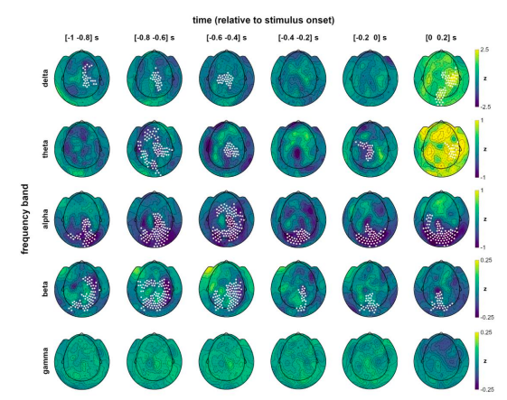
Fig. S4 | Band-specific topographies over time. Whole-scalp topographic distribution of normalised pre- and peristimulus power differences between hits and misses, separately for each frequency band. Channels with significant differences in the respective band are marked (cluster-corrected within the respective time frame). Related to Fig. 3.
Compared to the clear parieto-occipital topography of prestimulus alpha modulations, delta and theta effects were prominently shifted to anterior sensors, which renders their involvement in low-level visual processing highly unlikely. No significant effects were observed in the gamma range. In contrast, beta-band modulations were closest to the alpha effects in their topography, covering parietal as well as occipital sites. Although the size of normalised effects were markedly smaller in the beta band (compared to alpha frequencies, cf. colour scaling), the topographic distribution of prestimulus modulations as well as the spectral proximity of the two bands prompted further investigation of beta involvement. To this end, we computed the instantaneous correlation between individual beta power (over the respiration cycle) and respiratory phase, analogous to our main analysis shown in Fig. 4c. Consistent with the TFR analysis shown above, no significant correlation between oscillatory power and respiration time courses were found for delta, theta, and gamma bands. For the beta band, however, we found a significant correlation during the inspiratory phase, similar to the alpha correlation described in the main text (and shown for comparison in the new Supplementary Fig. S5):
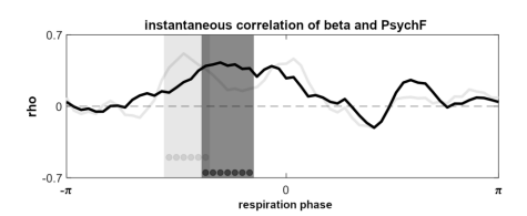
Fig. S5 | Instantaneous correlation of beta power and perceptual sensitivity. Group-level correlation between individual beta and PsychF threshold courses (averaged between 14 - 30 Hz) with significant phase vector (length of seven time points) marked by dark grey dots (cluster-corrected). Correlation time course of the alpha band (see Fig. 4c) shown for reference in light grey. Related to Fig. 4.
While both alpha and beta power were correlated to the breathing signal during the inspiratory phase, the correlation time courses suggested that there might be differential effects in both frequency bands, as indicated by the phase shift visible in Supplementary Fig S5. Therefore, we finally recomputed the LMEM visualised in Fig. 4 with an additional factor for beta power. In this extended model, significant effects were found for both alpha (t(1790) = 3.27, p < .001) and beta power (t(1790) = 4.83, p < .001). Beta showed significant interactions with the sine of the respiratory signal (t(1790) = -3.52, p < .001) as well as with alpha power (t(1790) = -4.63, p < .001). Comparing the LMEM to the previous model which only contained alpha power (along with respiratory sine and cosine) confirmed the significant contribution of beta power in explaining PsychF threshold variation by means of a theoretical likelihood ratio test (χ²(4) = 60.43, p < .001). Overall, we thus found beta power to be i) significantly modulated by respiration (see Fig 1), ii) significantly suppressed over parieto-occipital sensors for hits vs misses (see Fig. S4), and iii) significantly contribute to variations in PsychF threshold (see Fig S5). Collectively, these findings suggest differential roles of alpha and beta power, which we discuss in the main text as well as in the Supplementary Text:
“Whole-scalp control analyses across all frequency bands demonstrated that this topographical pattern was unique to alpha and beta prestimulus power (see Supplementary Text 1 and Fig. S4).”
“Control analyses across all frequency bands yielded a significant instantaneous correlation between PsychF threshold and beta power as well, albeit at a slightly later phase (see Fig. S5). No significant correlations were found for the remaining frequency bands.”
“Accordingly, one recent study proposed that the alpha rhythm shapes the strength of neural stimulus representations by modulating excitability (Iemi et al., 2021). Previous work by Michalareas and colleagues (2016) as well as our own data (see Supplementary Material) point towards an interactions between alpha and beta bands, as beta oscillations have very recently been implicated in mediating top-down signals from the frontal eye field (FEF) that modulate excitability in the visual cortex during spatial attention (Veniero et al., 2021). Our findings suggest that this top-down signalling is modulated across the respiration cycle in a way that changes behavioural performance.”
In the discussion the authors speculate that respiration locked modulation of alpha power and associated neuronal excitability could be based on the modulation of blood CO2 levels. Most recent studies of respiratory modulation of brain activity have demonstrated significant differences between nasal and oral breathing, with nasal breathing (through activation of the olfactory bulb) typically resulting in a stronger influence of respiration on neuronal activity and behavioral performance than oral breathing. The authors only tested nasal breathing. If blood CO2 fluctuations are indeed responsible for the observed effect, there should be no difference in outcome between nasal and oral breathing. Comparing the two conditions would thus provide interesting additional information about the possible underlying mechanisms.
We appreciate the reviewer’s well-justified remarks regarding the differential effects for nasal and oral breathing and their implications on underlying mechanisms such as CO2. In revising the present as well as other manuscripts, it has become evident that fluctuations of CO2 alone (and, as we previously discussed, related changes in pH) cannot possibly explain the effects we and others are observing. Therefore, the revised manuscript no longer discusses CO2 as a potential mechanism. We have removed the corresponding paragraph and instead refer to the distinction between nasal and oral breathing to strengthen the argument for OB-induced cross-frequency coupling:
“As outlined in the introduction, there is broad consensus that cross-frequency coupling (Canolty and Knight, 2010; Jensen and Colgin, 2007) plays a central role in translating respiratory to neural rhythms: Respiration entrains neural activity within the olfactory tract via mechanoreceptors, after which the phase of this infraslow rhythm is coupled to the amplitude of faster oscillations (see Fontanini and Bower, 2006; Ito et al., 2014). While this mechanism is difficult to investigate directly in humans, converging evidence for the importance of bulbar rhythms comes from animal bulbectomy studies (Ito et al., 2014) and the fact that respiration-related changes in both oscillatory power and behaviour dissipate during oral breathing (Zelano et al., 2016; Perl et al., 2019). Thus, rhythmic nasal respiration conceivably aligns rhythmic brain activity across the brain, which in turn influences behaviour. In our present paradigm, transient phases of heightened excitability would then be explained by decreased inhibitory influence on neural signalling within the visual cortex, leading to increased postsynaptic gain and higher detection rates. Given that the breathing act is under voluntary control, the question then becomes to what extent respiration may be actively used to synchronise information sampling with phasic states of heightened excitability.”
Reviewer #3 (Public Review):
The topic is timely, the study is well-designed, and the work has been performed in a highly competent manner. The authors relate three variables: respiration, alpha power and perceptual performance, constituting a link between somatic and neuronal physiology and cognition. A particular strength is the temporal resolution of respiration effects on cognition (continuous analysis of the respiration cycle). Furthermore, results are well contextualized by very comprehensively written introduction and discussion sections (which, nevertheless, could be slightly shortened).
We do appreciate the reviewer’s positive evaluation of our manuscript and are thankful for their constructive remarks. We respond to their comments in detail below and have shortened the Discussion section in response to one of the reviewer’s remarks (kindly see points 1.1 and 2 below).
I have three points of criticism, all meant in a constructive way:
- I wonder whether the authors could have gone one step further in the analysis of causal mechanisms, rather than correlations. The analysis of timing (Fig. 4d) and the last sentence of the abstract suggest that they imagine a causal role of respiratory feedback on cognitive performance, mediated via coordination of brain activity (in the specific case, by increasing excitability in visual areas). This could be made more explicit by appropriate experiments and data analysis:
1.1. Manipulating the input signal: former studies suggest that nasal respiration is crucial for effects on brain oscillations and/or performance (e.g. Yanovsky et al., 2014; Zelano et al., 2016). Thus, the causal inference could be easily checked by comparing nasal versus oral respiration, without changing gas- and pH-parameters of activity of brainstem centers. >Admittedly, this experiment may add significant work to the present data which, by themselves, are already very strong.
We thank the reviewer for their insightful comment regarding the question of causality. We acknowledge that our interpretation should have been phrased a little more cautiously. Therefore, we have rephrased corresponding paragraphs at various instances throughout the manuscript (kindly see below). Particular under current circumstances, we further appreciate the reviewer’s concern regarding the acquisition of additional data for a direct comparison of nasal vs oral breathing. Their comment is of course entirely valid and we were eager to address it, especially since it relates to CO2- and/or pH-related mechanisms of RMBOs we previously discussed. In light of the reviewer’s comments (also see their related comment #2 below) and convincing evidence from both animal and human studies that already compared nasal and oral breathing, we no longer feel that changes in CO2 provide a reasonable explanation for respiration-related oscillatory and behavioural effects we observed here. Consequently, we have removed the corresponding paragraph from the Discussion section which now reads as follows:
“As outlined in the introduction, there is broad consensus that cross-frequency coupling (Canolty and Knight, 2010; Jensen and Colgin, 2007) plays a central role in translating respiratory to neural rhythms: Respiration entrains neural activity within the olfactory tract via mechanoreceptors, after which the phase of this infraslow rhythm is coupled to the amplitude of faster oscillations (see Fontanini and Bower, 2006; Ito et al., 2014). While this mechanism is difficult to investigate directly in humans, converging evidence for the importance of bulbar rhythms comes from animal bulbectomy studies (Ito et al., 2014) and the fact that respiration-related changes in both oscillatory power and behaviour dissipate during oral breathing (Zelano et al., 2016; Perl et al., 2019). Thus, rhythmic nasal respiration conceivably aligns rhythmic brain activity across the brain, which in turn influences behaviour. In our present paradigm, transient phases of heightened excitability would then be explained by decreased inhibitory influence on neural signalling within the visual cortex, leading to increased postsynaptic gain and higher detection rates. Given that the breathing 17 act is under voluntary control, the question then becomes to what extent respiration may be actively used to synchronise information sampling with phasic states of heightened excitability.”
1.2. Temporal relations: The authors show that respiration-induced alpha modulation precedes behavioral modulation (Fig. 4d and related results text). Again, this finding suggests a causal influence of respiration on performance, mediated by alpha suppression (see results, lines 318-320). Could the data be directly tested for causality (e.g. by applying Granger causality, dynamic causal modelling or other methods)? If this is difficult, the question of causality should at least be discussed more explicitly.
We appreciate the reviewer’s constructive criticism and their suggestion to employ causal analyses. While we agree that the overall pattern of results strongly suggests a causal cascade of respiration -> excitability -> perception, our interpretation with regard to a dynamic mechanism was probably overly strong. Unfortunately, it is indeed difficult to use directional analyses like Granger causality or DCM on the current data, since these methods quantify the relationship between two time series. They would not allow us to investigate the triad of respiration, alpha power, and behaviour, as we have discrete responses (i.e., single events) instead of a continuous behavioural measure. In fact, we are currently preparing a directional analysis of respiration-brain coupling (in resting-state data without a behavioural component) for an upcoming manuscript. In response to the reviewer’s remarks, we have toned down our interpretation throughout the manuscript and explicitly discuss the question of causality in the Discussion section of the revised manuscript:
“The bootstrapping procedure yielded a confidence interval of [-33.17 -29.25] degrees for the peak effect of alpha power. While these results strongly suggest that respiration-alpha coupling temporally precedes behavioural consequences, they do not provide sufficient evidence for a strict causal interpretation (see Discussion)”
“Rigorous future work is needed to investigate potentially causal effects of respiration-brain coupling on behaviour, e.g. by means of directed connectivity within task-related networks. A second promising line of research considers top-down respiratory modulation as a function of stimulus characteristics (such as predictability). This would grant fundamental insights into whether respiration is actively adapted to optimise sensory sampling in different contexts, as suggested by the animal literature.”
- At various instances, the authors suggest that respiration-induced changes in pH may be responsible for the changes in cortical excitability which, in turn, affect behavioral performance. In the discussion, they quote respective literature (lines 406-418). I glanced through the quoted papers by Feldman, Chesler, Lee, Dulla and Gourine - as far as I could see none of them suggests that the cyclic process of respiration induces significant cyclic shifts of pH in the brain parenchyma (if at all, this may occur in specialized chemosensory neurons in the brainstem). Moreover, recent real-time measurements by Zhang et al. (Chem. Sci 12:7369-7376) do also not reveal such cyclic changes in the cortex. Finally, translating oscillatory extracellular pH changes (if existent) into changes in inhibitory efficacy would require some time, potentially inducing delays and variance onto the cyclic changes at the network level. I feel that the evidence for the proposed mechanism is not sufficient, notwithstanding that it is a valid hypothesis. Please check and correct the interpretation of the cited literature if necessary.
We acknowledge the reviewer’s caution regarding our suggestion of pH involvement, which is closely related to their previous comment (kindly see 1.1 above). As the reviewer mentions themselves, there are several studies demonstrating an absence of both neural and behavioural modulations for oral (vs nasal) breathing. These reports provide direct evidence against a mechanism driven by changes in CO2 and/or pH, which would be identical for nasal and oral breathing. Moreover, a second valid criticism is the uncertain temporal delay introduced by the (hypothetical) translation of pH changes into neural signals, which would most likely be incompatible with the ‘online’ (i.e., within-cycle) effects we report here. Therefore, as outlined in our response above, we have removed the pH-related suggestions from the Discussion section.
- Finally, some illustrations should be presented in a clearer way for those not familiar with the specifics of MEG analysis.
We appreciate the reviewer’s suggestions regarding the clarity of our manuscript.
Author Response:
Reviewer #1 (Public Review):
In this manuscript, the authors challenge the long-standing conclusion that Orco and IR-dependent olfactory receptor neurons are segregated into subtypes such that Orco and IR expression do not overlap. First, the authors generate new knock-in lines to tag the endogenous loci with an expression reporter system, QF/QUAS. They then compare the observed expression of these knock-ins with the widely used system of enhancer transgenes of the same receptors, namely Orco, IR8a, IR25a, and IR76b. Surprisingly, they observe an expansion of the expression of the individual knock-in reporters as compared to the transgenic reporters in more chemosensory neurons targeting more glomeruli per receptor type than previously reported. They verify the expression of the knock-in reporters with antibody staining, in situ hybridization and by mining RNA sequencing data.
Finally, they address the question of physiological relevance of such co-expression of receptor systems by combining optogenetic activation with single sensillum recordings and mutant analysis. Their data suggests that IR25a activation can modulate Orco-dependent signaling and activation of olfactory sensory neurons.
The paper is well written and easy to follow. The data are well presented and very convincing due in part to the combination of complementary methods used to test the same point. Thus, the finding that co-receptors are more broadly and overlappingly expressed than previously thought is very convincing and invites speculation of how this might be relevant for the animal and chemosensory processing in general. In addition, the new method to make knock-ins and the generated knock-ins themselves will be of interest to the fly community.
We thank the reviewer for their enthusiasm and support of our work!
The last part of the manuscript, although perhaps the most interesting, is the least developed compared to the other parts. In particular, the following points could be addressed:
- It would be good to see a few more traces and not just the quantifications. For instance, the trace of ethyl acetate in Fig. 6C, and penthyl acetate for 6G.
Thank you for the suggestion. We have added a new figure supplement (Figure 6-Figure Supplement 3) with additional example traces for all odorants from Figure 6 for which we found a statistically significant difference between the two genotypes (Ir25a versus wildtype).
- In Fig. 4D, the authors show the non-retinal fed control, which is great. An additional genetic control fed with retinal would have been nice.
For these experiments, we followed a standard practice in Drosophila optogenetics to test the same experimental genotype in the presence or absence of the essential cofactor all-trans-retinal. This controls for potential effects from the genetic background. It is possible our description of these experiments was unclear (as also suggested by comments from Reviewer 2). As such, we have clarified our experimental design for the optogenetic experiments in the revised manuscript:
Modified text: “No light-induced responses were found in control flies, which had the same genotype as experimental flies but were not fed all-trans retinal (-ATR), a necessary co-factor for channelrhodopsin function (see Methods).” and “Bottom trace is control animal, which has the same genotype as the experimental animal but was not fed the required all-trans retinal cofactor (-ATR).”
Figure 4-Figure Supplement 1 legend: “In all optogenetic experiments, control animals have the same genotypes as the corresponding experimental animals but have not been fed all-trans retinal.”
Methods: “For all optogenetic experiments, the control flies were of the same genotype as experimental flies but had not been fed all-trans retinal.”
- It appears that mostly IR25a is strongly co-expressed with other co-receptors. The provided experiments suggest a possible modulation between IR25a and Orco-dependent neuronal activity. However, what does this mean? How could this be relevant? And moreover, is this a feature of Drosophila melanogaster after many generations in laboratories?
We share this reviewer’s excitement regarding the numerous questions our work now raises. While testing additional functional ramifications of chemosensory co-receptor expression is beyond the scope of this work (but will undoubtedly be the focus of future studies), we did expand on what this might mean in the revised Discussion section of the revised manuscript. Previously, we had raised the hypothesis that chemoreceptor co-expression could be an evolutionary relic of Ir25a expression in all chemoreceptor neurons , or a biological mechanism to broaden the response profile of an olfactory neuron without sacrificing its ability to respond to specific odors. We now extend our discussion to raise additional possible ramifications. For example, we suggest that modulating Ir25a coexpression could alter the electrical properties of a neuron, making it more (or possibly less) sensitive to Orco-dependent responses. We also suggest that Ir25a coexpression might be an evolutionary mechanism to allow olfactory neurons to adjust their response activities. That is, that most Orco-positive olfactory neurons are already primed to be able to express a functional Ir receptor if one were to be expressed. Such co-expression in some olfactory neurons might present an evolutionary advantage by ensuring olfactory responses to a complex but crucial biologically relevant odor, like human odors to some mosquitoes.
Reviewer #2 (Public Review):
In the present study, the authors: 1) generated knock-in lines for Orco, Ir8a, Ir25a, and IR7ba, and examined their expression, with a main focus on the adult olfactory organs. 2) confirmed the expression of these receptors using antibody staining. 3) examined the innervation patterns of these knock-in lines in the nervous system. 4) identified a glomerulus, VM6, that is divided into three subdivisions. 5) examined olfactory responses of neurons co-expressing Orco and Ir25a
The results of the first four sets of experiments are well presented and support the conclusions, but the results of the last set of experiments (the electrophysiology part) need some details. Please find my detailed comments below.
We thank the reviewer for their support of our work and appreciating the importance of our findings. In the revised manuscript, we now provide the additional experimental details for the electrophysiology work as requested.
Major points
Line 167-171: I wonder if the authors also compared the Orco-T2A-QF2 knock-in with antibody staining of the antenna.
We did perform whole-mount anti-Orco antibody staining on Orco-T2A-QF2 > GFP antennae (example image below). We saw broad overlap between Orco+ and GFP+ cells, similar to the palps. However, we did not include these results since quantification of these tissues is challenging for the following reasons:
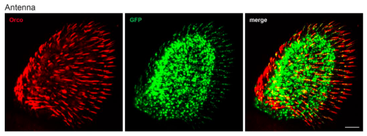
*Co-staining of anti-Orco and GFP in Orco-T2A-QF2 > 10xQUAS-6xGFP antenna *
Lines 316-319 (Figure 4D): It would be better if the authors compare the responses of Ir25a>CsChrimson to those of Orco>CsChrimson.
The goal of the optogenetic experiments was to provide experimental support for Ir25a expression in Orco+ neurons in an approach independent to previous methods. Our main question was whether we could activate what was previously considered Orco-only olfactory neurons using the Ir25a knock-in. These experiments were not designed to determine if this optogenetic activation recapitulated the normal activity of these neurons. For these reasons, we did not attempt the optogenetic experiments with Orco>CsChrimson flies.
Line 324-326: Why the authors tested control flies not fed all-trans retinal? They should test Ir25a-T2A-QF2>QUAS-CsChrimson not fed all-trans retinal as a control.
We apologize for the confusion. The “control” flies we used were indeed Ir25a-T2AQF2>QUAS-CsChrimson flies not fed all-trans retinal as suggested by the reviewer. This detail was in the methods, yet likely was not clear. We have amended the main text in multiple locations to state the full genotype of the control fly more clearly:
Modified text: “No light-induced responses were found in control flies, which had the same genotype as experimental flies but were not fed all-trans retinal (-ATR), a necessary co-factor for channelrhodopsin function (see Methods).” and “Bottom trace is control animal, which has the same genotype as the experimental animal but was not fed the required all-trans retinal cofactor (-ATR).”
Figure 4-Figure Supplement 1 legend: “In all optogenetic experiments, control animals have the same genotypes as the corresponding experimental animals but have not been fed all-trans retinal.”
Methods: “For all optogenetic experiments, the control flies were of the same genotype as experimental flies but had not been fed all-trans retinal.”
Line 478-500: I wonder if the observed differences between the wildtype and Ir25a2 mutant lines are due to differences in the genetic background between both lines. Did the authors backcross Ir25a2 mutant line with the used wildtype for at least five generations?
Yes, the mutants are outcrossed into the same genetic background as the wildtypes for at least five generations. Please see Methods, revised manuscript: “Ir25a2 and Orco2 mutant fly lines were outcrossed into the w1118 wildtype genetic background for at least 5 generations.”
Line 1602-1603: Does the identification of ab3 sensilla using fluorescent-guided SSR apply for ab3 sensilla in Orco mutant flies. How does this ab3 fluorescent-guided SSR work?
In fluorescence guided SSR (fgSSR; Lin and Potter, PloS One, 2015), the ab3 sensilla is GFPlabelled (genotype: Or22a-Gal4>UAS-mCD8:GFP), which allows this sensilla to be specifically identified under a microscope and targeted for SSR recordings. We generated fly stocks for fgSSR identification of ab3 in all three genetic backgrounds (wildtype, Orco mutant, Ir25a mutant).
These three genotypes are described in the methods:
“Full genotypes for ab3 fgSSR were:
Pin/CyO; Or22a-Gal4,15XUAS-IVS-mcd8GFP/TM6B (wildtype),
Ir25a2; Or22a-Gal4,15XUAS-IVS-mcd8GFP/TM6B (Ir25a2 mutant),
Or22a-Gal4/10XUAS-IVS-mcd8GFP (attp40); Orco2 (Orco2 mutant).”
Line 1602-1604: There is no mention of how the authors identified ab9 sensilla.
Information on the identification of ab9 sensilla is under the optogenetics section of the methods: “Identification of ab9 sensilla was assisted by fluorescence-guided Single Sensillum Recording (fgSSR) (Lin and Potter, 2015) using Or67b-Gal4 (BDSC #9995) recombined with 15XUAS-IVS-mCD8::GFP (BDSC #32193).”
Line 1648: what are the set of odorants that were used to identify the different coeloconic sensilla?
We have added the specific odorants used for sensillar identification for coeloconic SSR in the Methods. The protocol and odorants used were:
*2,3-butanedione (BUT), 1,4-diaminobutane (DIA), Ammonia (AM), hexanol (HEX), phenethylamine (PHEN), and propanal (PROP) to distinguish coeloconic sensilla:
o Wildtype flies: Strong DIA and BUT responses identify ac2 and rule out ac4. Absence of strong AM response rules out ac1, absence of HEX response rules out ac3, absence of PHEN response further rules out ac4.
o Ir25a mutant flies (amine responses lost, so cannot use PHEN and DIA as diagnostics): Strong BUT response and moderate PROP response identify ac2 and rule out ac4. Absence of strong AM response rules out ac1, absence of HEX response rules out ac3. Ac4 is further ruled out anatomically based on sensillar location compared to ac2.
Revised text: “Different classes of coeloconic sensilla were identified by their known location on the antenna and confirmed with their responses to a small panel of diagnostic odorants: in wildtype flies, ac2 sensilla were identified by their strong responses to 1,4-diaminobutane and 2,3-butanedione. The absence of a strong response to ammonia was used to rule out ac1 sensilla, the absence of a hexanol response was used to rule out ac3 sensilla, and the absence of a phenethylamine response was used to rule out ac4 sensilla. In Ir25a mutant flies in which amine responses were largely abolished, ac2 and ac4 sensilla were distinguished based on anatomical location, as well as the strong response of ac2 to 2,3-butanedione and the moderate response to propanal (both absent in ac4). Ac1 and ac3 sensilla were excluded similarly in the mutant and wildtype flies. No more than 4 sensilla per fly were recorded. Each sensillum was tested with multiple odorants, with a rest time of at least 10s between applications.
Author Response:
Reviewer #1 (Public Review):
- There was little comment on the strategy/mechanism that enabled subjects to readily attain Target I (MU 1 active alone), and then Target II (MU1 and MU2 active to the same relative degree). To accomplish this, it would seem that the peak firing rate of MU1 during pursuit of Target II could not exceed that during Target I despite an increased neural drive needed to recruit MU2. The most plausible explanation for this absence of additional rate coding in MU1 would be that associated with firing rate saturation (e.g., Fuglevand et al. (2015) Distinguishing intrinsic from extrinsic factors underlying firing rate saturation in human motor units. Journal of Neurophysiology 113, 1310-1322). It would be helpful if the authors might comment on whether firing rate saturation, or other mechanism, seemed to be at play that allowed subjects to attain both targets I and II.
To place the cursor inside TII, both MU1 and MU2 must discharge action potentials at their corresponding average discharge rate during 10% MVC (± 10% due to the target radius and neglecting the additional gain set manually in each direction). Therefore, subjects could simply exert a force of 10% MVC to reach TII and would successfully place the cursor inside TII. However, to get to TI, MU1 must discharge action potentials at the same rate as during TII hits (i.e. average discharge rate at 10% MVC) while keeping MU2 silent. Based on the performance analysis in Fig 3D, subjects had difficulties moving the cursor towards TI when the difference in recruitment threshold between MU1 and MU2 was small (≤ 1% MVC). In this case, the average discharge rate of MU1 during 10% MVC could not be reached without activating MU2. As could be expected, reaching towards TI became more successful when the difference in recruitment threshold between MU1 and MU2 was relatively large (≥3% MVC). In this case, subjects were able to let MU1 discharge action potentials at its average discharge rate at 10% MVC without triggering activation of MU2 (it seems the discharge rate of MU1 saturated before the onset of MU2). Such behaviour can be observed in Fig. 2A. MUs with a lower recruitment threshold saturate their discharge rate before the force reaches 10% MVC. We adapted the Discussion accordingly to describe this behaviour in more detail.
- Figure 4 (and associated Figure 6) is nice, and the discovery of the strategy used by subjects to attain Target III is very interesting. One mechanism that might partially account for this behavior that was not directly addressed is the role inhibition may have played. The size principle also operates for inhibitory inputs. As such, small, low threshold motor neurons will tend to respond to a given amount of inhibitory synaptic current with a greater hyperpolarization than high threshold units. Consequently, once both units were recruited, subsequent gradual augmentation of synaptic inhibition (concurrent with excitation and broadly distributed) could have led to the situation where the low threshold unit was deactivated (because of the higher magnitude hyperpolarization), leaving MU2 discharging in isolation. This possibility might be discussed.
We agree with the reviewer’s comment that inhibition might have played a critical role in succeeding to reach TIII. Hence, we have added this concept to our discussion.
- In a similar vein as for point 2 (above), the argument that PICs may have been the key mechanism enabling the attainment of target III, while reasonable, also seems a little hand wavy. The problem with the argument is that it depends on differential influences of PICs on motor neurons that are 1) low threshold, and 2) have similar recruitment thresholds. This seems somewhat unlikely given the broad influence of neuromodulatory inputs across populations of motor neurons.
We agree with the reviewer’s point and reasoning that a mixture of neuromodulation and inhibition likely introduced the variability in MU activity we observed in this study. This comment is addressed in the answer to comment 3.
Reviewer #2 (Public Review):
[...]
- Some subjects seemed to hit TIII by repeatedly "pumping" the force up and down to increase the excitability of MU2 (this appears to happen in TIII trials 2-6 in Fig. 4 - c.f. p18 l30ff). It would be useful to see single-trial time series plots of MU1, MU2, and force for more example trials and sessions, to get a sense for the diversity of strategies subjects used. The authors might also consider providing additional analyses to test whether multiple "pumps" increased MU2 excitability, and if so, whether this increase was usually larger for MU2 than MU1. For example, they might plot the ratio of MU2 (and MU1) activation to force (or, better, the residual discharge rate after subtracting predicted discharge based on a nonlinear fit to the ramp data) over the course of the trial. Is there a reason to think, based on the data or previous work, that units with comparatively higher thresholds (out of a sample selected in the low range of <10% MVC) would have larger increases in excitability?
We added a supplementary figure (Supplement 4) that visualizes additional trials from different conditions and subjects for TIII-instructed trials and noted this in the text.
MU excitability might indeed be pronounced during repeated activations within a couple of seconds (see, for example, M. Gorassini, J. F. Yang, M. Siu, and D. J. Bennett, “Intrinsic Activation of Human Motoneurons: Reduction of Motor Unit Recruitment Thresholds by Repeated Contractions,” J. Neurophysiol., vol. 87, no. 4, pp. 1859–1866, 2002.). Such an effect, however, seems to be equally distributed to all active MUs. Moreover, we are not aware of any recent studies suggesting that MUs, within the narrow range of 0-10% MVC, may be excited differently by such a mechanism. Supplement 4C and D illustrate trials in which subjects performed multiple “pumps”. Visually, we could not find changes in the excitability specific to any of the two MUs nor that subjects explored repeated activation of MUs as a strategy to reach TIII. It seems subjects instead tried to find the precise force level which would allow them to keep MU2 active after the offset of MU1. We further discussed that PICs act very broadly on all MUs. The observed discharge patterns when successfully reaching TIII may likely be due to an interplay of broadly distributed neuromodulation and locally acting synaptic inhibition.
- I am somewhat surprised that subjects were able to reach TIII at all when the de-recruitment threshold for MU1 was lower than the de-recruitment threshold for MU2. It would be useful to see (A) performance data, as in Fig. 3D or 5A, conditioned on the difference in de-recruitment thresholds, rather than recruitment thresholds, and (B) a scatterplot of the difference in de-recruitment vs the difference in recruitment thresholds for all pairs.
We agree that comparing the difference in de-recruitment threshold with the performance of reaching each target might provide valuable insights into the strategies used to perform the tasks. Hence, we added this comparison to Figure 4E at p. 16, l. 1. A scatterplot of the difference in de-recruitment threshold and the difference in recruitment threshold has been added to Supplement 3A. The Results section was modified in line with the above changes.
- Using MU1 / MU2 rates to directly control cursor position makes sense for testing for independent control over the two MUs. However, one might imagine that there could exist a different decoding scheme (using more than two units, nonlinearities, delay coordinates, or control of velocity instead of position) that would allow subjects to generate smooth trajectories towards all three targets. Because the authors set their study in a BCI context, they may wish to comment on whether more complicated decoding schemes might be able to exploit single-unit EMG for BCI control or, alternatively, to argue that a single degree of freedom in input fundamentally limits the utility of such schemes.
This study aimed to assess whether humans can learn to decorrelate the activity between two MUs coming from the same functional MU pool during constraint isometric conditions. The biofeedback was chosen to encourage subjects to perform this non-intuitive and unnatural task. Transferring biofeedback on single MUs into an application, for example, BCI control, could include more advanced pre-processing steps. Not all subjects were able to navigate the cursor along both axes consistently (always hitting TI and TIII). However, the performance metric (Figure 4C) indicated that subjects became better over time in diverging from the diagonal and thus increased their moving range inside the 2D space for various combinations of MU pairs. Hence, a weighted linear combination of the activity of both MUs (for example, along the two principal components based on the cursor distribution) may enable subjects to navigate a cursor from one axis to another. Similarly, coadaptation methods or different types of biofeedback (auditory or haptic) may help subjects. Furthermore, using only two MUs to drive a cursor inside a 2-D space is prone to interference. Including multiple MUs in the control scheme may improve the performance even in the presence of noise. We have shown that the activation of a single MU pool exposed to a common drive does not necessarily obey rigid control. State-dependent flexible control due to variable intrinsic properties of single MUs may be exploited for specific applications, such as BCI. However, further research is necessary to understand the potentials and limits of such a control scheme.
- The conclusions of the present work contrast somewhat with those of Marshall et al. (ref. 24), who claim (for shoulder and proximal arm muscles in the macaque) that (A) violations of the "common drive" hypothesis were relatively common when force profiles of different frequencies were compared, and that (B) microstimulation of different M1 sites could independently activate either MU in a pair at rest. Here, the authors provide a useful discussion of (A) on p19 l11ff, emphasizing that independent inputs and changes in intrinsic excitability cannot be conclusively distinguished once the MU has been recruited. They may wish to provide additional context for synthesizing their results with Marshall et al., including possible differences between upper / lower limb and proximal / distal muscles, task structure, and species.
The work by Marshall, Churchland and colleagues shows that when stimulating focally in specific sites in M1 single MUs can be activated, which may suggest a direct pathway from cortical neurons to single motor neurons within a pool. However, it remains to be shown if humans can learn to leverage such potential pathways or if the observations are limited to the artificially induced stimulus. The tibialis anterior receives a strong and direct cortical projection. Thus, we think that this muscle may be well suited to study whether subjects can explore such specific pathways to activate single MUs independently. However, it may very well be that the control of upper limbs show more flexibility than lower ones. However, we are not aware of any study that may provide evidence for a critical mismatch in the control of upper and lower limb MU pools. We have added this discussion to the manuscript.
Reviewer #3 (Public Review):
[...]
Even if the online decomposition of motor units were performed perfectly, the visual display provided to subject smooths the extracted motor unit discharge rates over a very wide time window: 1625 msec. This window is significantly larger than the differences in recruitment times in many of the motor unit pairs being used to control the interface. So while it's clear that the subjects are learning to perform the task successfully, it's not clear to me that subjects could have used the provided visual information to receive feedback about or learn to control motor unit recruitment, even if individuated control of motor unit recruitment by the nervous system is possible. I am therefore not convinced that these experiments were a fair test of subjects' ability to control the recruitment of individual motor units.
Regarding the validating of isolating motor units in the conditions analysed in this study, we have added a full new set of measurements with concomitant surface and intramuscular recordings during recruitment/derecruitment of motor units at variable recruitment speed. This provides a strong validation of the approach and of the accuracy of the online decomposition used in this study. Subjects received visual feedback on the activity of the selected MU pair, i.e. discharge behaviour of both MUs and the resulting cursor movement. This information was not clear from the initial submission and hence, we annotated the current version to clarify the biofeedback modalities. To further clarify the decoding of incoming MU1/MU2 discharge rates into cursor movement, we included Supplement 2. We also included a video that shows that the smoothing window on the cursor position does not affect the immediate cursor movement due to incoming spiking activity. For example, as shown in Supplement 2, for the initial offset of 0ms, the cursor starts moving along the axis corresponding to a sole activation of MU1 and immediately diverges from this axis when MU2 starts to discharge action potentials. We, therefore, think that the biofeedback provided to the subjects does allow exploration of single MU control.
Along similar lines, it seems likely to me that subjects are using some other strategy to learn the task, quite possibly one based on control of over overall force at the ankle and/or voluntary recruitment of other leg/foot muscles. Each of these variables will presumably be correlated with the activity of the recorded motor units and the movement of the cursor on the screen. Moreover, because these variables likely change on a similar (or slower) timescale than differences in motor units recruitment or derecruitment, it seems to me that using such strategies, which do not reflect or require individuated motor unit recruitment, is a highly effective way to successfully complete the task given the particular experimental setup.
In addition to being seated and restricted by an ankle dynamometer, subjects were instructed to only perform dorsiflexion of the ankle. Further, none of the subjects reported compensatory movements as a strategy to reach any of the targets. In addition, to be successfully utilised, such compensatory movements would need to influence various combinations of MUs tested in this study equally, even when they differ in size. Nevertheless, we acknowledge, as pointed out by the reviewer, that our setup has limitations. We only measured force in a single direction (i.e. ankle dorsiflexion) and did not track toe, hip or knee movements. Even though an instructor supervised leg movement throughout the experiment, it may be that very subtle and unknowingly compensatory movements have influenced the activity of the selected MUs. Hence, we updated the limitations section in the Discussion.
To summarize my above two points, it seems like the author's argument is that absence of evidence (subjects do not perform individuated MU recruitment in this particular task) constitutes evidence of absence (i.e. is evidence that individuated recruitment is not possible for the nervous system or for the control of brain-machine interfaces). Therefore given the above-described issues regarding real-time feedback provided to subjects in the paper it is not clear to me that any strong conclusions can be drawn about the nervous system's ability or inability to achieve individuated motor unit recruitment.
We hope that the above changes clarify the biofeedback modalities and their potential to provide subjects with the necessary information for exploring independent MU control. Our experiments aimed to investigate whether subjects can learn under constraint isometric conditions to decorrelate the activity between two MUs coming from the same functional pool. While it seemed that MU activity could be decorrelated, this almost exclusively happened (TIII-instructed trials) within a state-dependent framework, i.e. both MUs must be activated first before the lower threshold one is switched off. We did not observe flexible MU control based exclusively on a selective input to individual MUs (MU2 activated before MU1 during initial recruitment). That does not mean that such control is impossible. However, all successful control strategies that were voluntarily explored by the subjects to achieve flexible control were based on a common input and history-dependent activation of MUs. We have added these concepts to the discussion section.
Second, to support the claims based on their data the authors must explain their online spike-sorting method and provide evidence that it can successfully discriminate distinct motor unit onset/offset times at the low latency that would be required to test their claims. In the current manuscript, authors do not address this at all beyond referring to their recent IEEE paper (ref [25]). However, although that earlier paper is exciting and has many strengths (including simultaneous recordings from intramuscular and surface EMGs), the IEEE paper does not attempt to evaluate the performance metrics that are essential to the current project. For example, the key metric in ref 25 is "rate-of-agreement" (RoA), which measures differences in the total number of motor unit action potentials sorted from, for example, surface and intramuscular EMG. However, there is no evaluation of whether there is agreement in recruitment or de-recruitment times (the key variable in the present study) for motor units measured both from the surface and intramuscularly. This important technical point must be addressed if any conclusions are to be drawn from the present data.
We have taken this comment in high consideration, and we have performed a validation based on concomitant intramuscular and surface EMG decomposition in the exact experimental conditions of this study, including variations in the speed of recruitment and de-recruitment. This new validation fully supports the accuracy in of the methods used when detecting recruitment and de-recruitment of motor units.
My final concern is that the authors' key conclusion - that the nervous system cannot or does not control motor units in an individuated fashion - is based on the assumption that the robust differences in de-recruitment time that subjects display cannot be due to differences in descending control, and instead must be due to changes in intrinsic motor unit excitability within the spinal cord. The authors simply assert/assume that "[derecruitment] results from the relative intrinsic excitability of the motor neurons which override the sole impact of the receive synaptic input". This may well be true, but the authors do not provide any evidence for this in the present paper, and to me it seems equally plausible that the reverse is true - that de-recrutiment might influenced by descending control. This line of argumentation therefore seems somewhat circular.
When subjects were asked to reach TIII, which required the sole activation of a higher threshold MU, subjects almost exclusively chose to activate both MUs first before switching off the lower threshold MU. It may be that the lower de-recruitment threshold of MU2 was determined by descending inputs changing the excitability of either MU1 or MU2 (for example, see J. Nielsen, C. Crone, T. Sinkjær, E. Toft, and H. Hultborn, “Central control of reciprocal inhibition during fictive dorsiflexion in man,” Exp. brain Res., vol. 104, no. 1, pp. 99–106, Apr. 1995 or E. Jankowska, “Interneuronal relay in spinal pathways from proprioceptors,” Prog. Neurobiol., vol. 38, no. 4, pp. 335–378, Apr. 1992). Even if that is the case, it remains unknown why such a command channel that potentially changes the excitability of a single MU was not voluntarily utilized at the initial recruitment to allow for direct movement towards TIII (as direct movement was preferred for TI and TII). We cannot rule out that de-recruitment was affected by selective descending commands. However, our results match observations made in previous studies on intrinsic changes of MU excitability after MU recruitment. Therefore, even if descending pathways were utilized throughout the experiment to change, for example, MU excitability, subjects were not able to explore such pathways to change initial recruitment and achieve general flexible control over MUs. The updated discussion explains this line of reasoning.
Reviewer #4 (Public Review):
[...]
- Figure 6a nicely demonstrates the strategy used by subjects to hit target TIII. In this example, MU2 was both recruited and de-recruited after MU1 (which is the opposite of what one would expect based on the standard textbook description). The authors state (page 17, line 15-17) that even in the reverse case (when MU2 is de-recruited before MU1) the strategy still leads to successful performance. I am not sure how this would be done. For clarity, the authors could add a panel similar to panel A to this figure but for the case where the MU pairs have the opposite order of de-recruitment.
We have added more examples of successful TIII-instructed trials in Supplement 4. Supplement 4C and D illustrate examples of subjects navigating the cursor inside TIII even when MU2 was de-recruited before MU1. As exemplarily shown, subjects also used the three-stage approach discussed in the manuscript. In contrast to successful trials in which MU2 was de-recruited after MU1 (for example, Supplement 4B), subjects required multiple attempts until finding a precise force level that allowed a continuous firing of MU2 while MU1 remained silent. We have added a possible explanation for such behaviour in the Discussion.
- The authors discuss a possible type of flexible control which is not evident in the recruitment order of MUs (page 19, line 27-28). This reasoning was not entirely clear to me. Specifically, I was not sure which of the results presented here needs to be explained by such mechanism.
We have shown that subjects can decorrelate the discharge activity of MU1 and MU2 once both MUs are active (e.g. reaching TIII). Thus, flexible control of the MU pair was possible after the initial recruitment. Therefore, this kind of control seems strongly linked to a specific activation state of both MUs. We further elaborated on which potential mechanisms may contribute to this state-dependent control.
- The authors argue that using a well-controlled task is necessary for understanding the ability to control the descending input to MUs. They thus applied a dorsi-flexion paradigm and MU recordings from TA muscles. However, it is not clear to what extent the results obtained in this study can be extrapolated to the upper limb. Controlling the MUs of the upper limb could be more flexible and more accessible to voluntary control than the control of lower limb muscles. This point is crucial since the authors compare their results to other studies (Formento et al., bioRxiv 2021 and Marshall et al., bioRxiv 2021) which concluded in favor of the flexible control of MU recruitment. Since both studies used the MUs of upper limb muscles, a fair comparison would involve using a constrained task design but for upper limb muscles.
We agree with the reviewer that our work differs from previous approaches, which also studied flexible MU control. We, therefore, added a paragraph to the limitation section of the Discussion.
- The authors devote a long paragraph in the discussion to account for the variability in the de-recruitment order. They mostly rely on PIC, but there is no clear evidence that this is indeed the case. Is it at all possible that the flexibility in control over MUs was over their recruitment threshold? Was there any change in de-recruitment of the MUs during learning (in a given recording session)?
The de-recruitment threshold did not critically change when compared before and after the experiment on each day (difference in de-recruitment threshold before and after the experiment: -0.16 ± 2.28% MVC, we have now added this result to the Results section). Deviations from the classical recruitment order may be achieved by temporal (short-lived) changes in the intrinsic excitability of single MUs. We, therefore, extended our discussion on potential mechanisms that may explain the observed variability given all MUs receive the same common input.
- The need for a complicated performance measure (define on page 5, line 3-6) is not entirely clear to me. What is the correlation between this parameter and other, more conventional measures such as total-movement time or maximal deviation from the straight trajectory? In addition, the normalization process is difficult to follow. The best performance was measured across subjects. Does this mean that single subject data could be either down or up-regulated based on the relative performance of the specific subject? Why not normalize the single-subject data and then compare these data across subjects?
We employed this performance metric to overcome shortcomings of traditional measures such as target hit count, time-to-target or deviation from the straight trajectory. Such problems are described in the illustration below for TIII-instructed trials (blue target). A: the duration of the trial is the same in both examples (left and right); however, on the left, the subject manages to keep the cursor close to the target-of-interest while on the right, the cursor is far away from the target centre of TIII. B: In both images the cursor has the same distance d to the target centre of TIII. However, on the left, the subject manages to switch off MU1 while keeping MU2 active, while on the right, both MUs are active. C: On the left, the subject manages to move the cursor inside the TIII before the maximum trial time was reached, while on the right, the subject moved the cursor up and down, not diverging from the ideal trajectory to the target centre but fails to place the cursor inside TIII within the duration of the trial. In all examples, using only one conventional measure fails to account for a higher performance value in the left scenario than in the right. Our performance metric combines several performance metrics such as time-to-target, distance from the target centre, and the discharge rate ratio between MU1 and MU2 via the angle 𝜑 and thus allows a more detailed analysis of the performance than conventional measures. The normalisation of the performance value was done to allow for a comparison across subjects. The best and worst performance was estimated using synthetic data mimicking ideal movement towards each target (i.e. immediate start from the target origin to the centre of the target, while the normalised discharge rate of the corresponding MU is set to 1). Since the target space is normalised for all subjects in the same manner (mean discharge rate of the corresponding MUs at 10 %MVC) this allows us to compare the performance between subjects, conditions and targets.
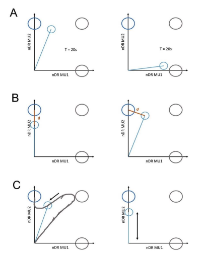
- Figure 3C appears to indicate that there was only moderate learning across days for target TI and TII. Even for target TIII there was some improvement but the peak performance in later days was quite poor. The fact that the MUs were different each day may have affected the subjects' ability to learn the task efficiently. It would be interesting to measure the learning obtained on single days.
We have added an analysis that estimated the learning within a session per subject and target (Supplement 3C). In order to evaluate the strength of learning within-session, the Spearman correlation coefficient between target-specific performance and consecutive trials was calculated and averaged across conditions and days. The results suggest that there was little learning within sessions and no significant difference between targets. These results have now been added to the manuscript.
- On page 16 line 12-13, the authors describe the rare cases where subjects moved directly towards TIII. These cases apparently occurred when the recruitment threshold of MU2 was lower. What is the probable source of this lower recruitment level in these specific trials? Was this incidental (i.e., the trial was only successful when the MU threshold randomly decreased) or was there volitional control over the recruitment threshold? Did the authors test how the MU threshold changed (in percentages) over the course of the training day?
We did not track the recruitment threshold throughout the session but only at the beginning and end. We could not identify any critical changes in the recruitment order (see Results section). However, our analysis indicated that during direct movements towards TIII, MU2 (higher threshold MU) was recruited at a lower force level during the initial ramp and thus had a temporary effective recruitment threshold below MU1. It is important to note that these direct movements towards TIII only occurred for pairs of MUs with a similar recruitment threshold (see Figure 6). One possible explanation for this temporal change in recruitment threshold could be altered excitability due to neuromodulatory effects such as PICs (see Discussion). We have added an analysis that shows that direct movements towards TIII occurred in most cases (>90%) after a preceding TII- or TIIIinstructed trial. Both of these targets-of-interest require activation of MU2. Thus, direct movement towards TIII was likely not the result of specific descending control. Instead, this analysis suggests that the PIC effect triggered at the preceding trial was not entirely extinguished when a trial ending in direct movement towards TIII started. Alternatively, the rare scenarios in which direct movements happened could be entirely random. Similar observations were made in previous biofeedback studies [31]. To clarify these points, we altered the manuscript.
Reviewer #2 (Public review):
This study conducted by Lu et al. explores the molecular underpinnings of sexual dimorphism in antiviral immunity in zebrafish, with a particular emphasis on the male-biased gene cyp17a2. The authors demonstrate that male zebrafish exhibit stronger antiviral responses than females, and they identify a teleost-specific gene cyp17a2 as a key regulator of this dimorphism. Utilizing a combination of in vivo and in vitro methodologies, they demonstrate that Cyp17a2 potentiates IFN responses by stabilizing STING via K33-linked polyubiquitination and directly degrades the viral P protein via USP8-mediated deubiquitination. The work challenges conventional views of sex-based immunity and proposes a novel, hormone- and sex chromosome-independent mechanism.
Strengths:
(1) The following constitutes a novel concept, sexual dimorphism in immunity can be driven by an autosomal gene rather than sex chromosomes or hormones represents a significant advance in the field, offering a more comprehensive understanding of immune evolution.
(2) The present study provides a comprehensive molecular pathway, from gene expression to protein-protein interactions and post-translational modifications, thereby establishing a link between Cyp17a2 and both host immune enhancement (via STING) and direct antiviral activity (via viral protein degradation).
(3) In order to substantiate their claims, the authors utilize a wide range of techniques, including transcriptomics, Co-IP, ubiquitination assays, confocal microscopy, and knockout models.
(4) The utilization of a singular model is imperative. Zebrafish, which are characterized by their absence of sex chromosomes, offer a clear genetic background for the dissection of autosomal contributions to sexual dimorphism.
Weaknesses:
(1) Limited discussion on whether this mechanism extends beyond Cyprinidae and its implications for teleost adaptation.
Comments on revisions:
The authors successfully achieved their primary aim, which was to identify and characterize a male-biased gene governing antiviral sexual dimorphism in fish. The data provide robust support for the conclusion that Cyp17a2 enhances antiviral immunity through dual mechanisms, STING stabilization and viral protein degradation, independent of classical sex-determining pathways. The findings are consistent across a range of experimental setups and are statistically robust. The revisions have significantly enhanced the clarity, depth, and overall quality of the manuscript. The authors have addressed each concern meticulously, resulting in a much-improved and robust article. No further suggestions are offered.
Author response:
The following is the authors’ response to the original reviews.
Reviewer #1 (Public review):
Weaknesses:
(1) Figure 10 outlines a mechanistic link between cyp17a2 and the sexual dimorphism the authors report for SVCV infection outcomes. The data presented on increased susceptibility of cyp17a2-/- mutant male zebrafish support this diagram, but this conclusion is fairly weak without additional experimentation in both males and females. The authors justify their decision to focus on males by stating that they wanted to avoid potential androgen-mediated phenotypes in the cpy17a2 mutant background (lines 152156), but this appears to be speculation. It also doesn't preclude the possibility of testing the effects of increased cyp17a2 expression on viral infection in both males and females. This is of critical importance if the authors intend to focus the study on sexual dimorphism, which is how the introduction and discussion are currently structured.
Thank you for your suggestion. We have revised the relevant statements in the introduction and discussion sections accordingly. The cyp17a2 overexpression experiments were not conducted in both male and female individuals was primarily based on two reasons. First, our laboratory currently lacks the technical capability to achieve cyp17a2 overexpression at the organismal level, existing methodologies are limited to gene knockout via CRISPR-Cas9. Second, even if overexpression were feasible, subsequent comparisons would need to be restricted within sexes (i.e., female vs. female controls or male vs. male controls) to eliminate potential confounding effects of sex hormones. Such experimental outcomes would only demonstrate the antiviral function of Cyp17a2 itself rather than directly elucidate mechanisms underlying sexual dimorphism, which diverges from the central objective of this study.
We fully agree with your perspective and have accordingly refined relevant discussions in the revised manuscript. Our conclusions now emphasize that "cyp17a2 is one of the factors contributing to sex-based differences in antiviral immunity" rather than implying that it "solely mediates the entire phenotypic divergence." These modifications have been incorporated into the resubmitted version (Lines 112-115).
(2) The authors present data indicating an unexpected link between cyp17a2 and ubiquitination pathways. It is unclear how a CYP450 family member would carry out such activities, and this warrants much more attention. One brief paragraph in the discussion (starting at line 448) mentions previous implications of CYP450 proteins in antiviral immunity, but given that most of the data presented in the paper attempt to characterize cyp17a2 as a direct interactor of ubiquitination factors, more discussion in the text should be devoted to this topic. For example, are there any known domains in this protein that make sense in this context? Discussion of this interface is more relevant to the study than the general overview of sexual dimorphism that is currently highlighted in the discussion and throughout the text.
We are grateful to the reviewer for their suggestion to elaborate on this novel finding. The discussion on this point has been expanded significantly (Lines 448-460). It is acknowledged that Cyp17a2 is devoid of the canonical domains that are typically associated with the ubiquitination machinery (e.g., RING, U-box). The present study proposes that the endoplasmic reticulum (ER) localization of Cyp17a2, in conjunction with its capacity to function as a scaffold protein, is of paramount significance. By residing in the ER, Cyp17a2 is strategically positioned to interact with key immune regulators such as STING, which also localizes to the ER. It is hypothesized that Cyp17a2 facilitates the recruitment of E3 ligases (btr32) and deubiquitinates (USP8) to their substrates (STING and SVCV P protein, respectively) by providing a platform for protein-protein interactions, rather than directly catalyzing ubiquitination. This noncanonical, scaffolding role for a cytochrome P450 (CYP450) enzyme represents an exciting evolutionary adaptation in teleost immunity.
(3) Figures 2-9 contain information that could be streamlined to highlight the main points the authors hope to make through a combination of editing, removal, and movement to supplemental materials. There is a consistent lack of clarity in these figures that could be improved by supplementing them with more text to accompany the supplemental figures. Using Figure 2 and an example, panel (A) could be removed as unnecessary, panel (B) could be exchanged for a volcano plot with examples highlighting why cyp17a2 was selected for further study and also the full dataset could be shared in a supplemental table, panel (C) could be modified to indicate why that particular subset was chosen for plotting along with an explanation of the scaling, panel (D) could be moved to supplemental because the point is redundant with panels (A) and (C), panel (E) could be presented as a heatmap, in panels (G) and (H) data from EPC cells could be moved to supplemental because it is not central to the phenotype under investigation, panels (J) to (L) and (N) to (P) could be moved to supplemental because they are redundant with the main points made in panels (M) and (Q). Similar considerations could be made with Figures 3-9.
We thank the reviewer for these excellent suggestions to improve the clarity and focus of our figures. A comprehensive review of all figures has been conducted in accordance with the recommendations made. Figure 2A has been removed. Figure 2B (revised Figure 2A) has been replaced with a volcano plot highlighting cyp17a2 and the full dataset has been provided as supplementary Table S2. Figure 2C (revised Figure 2B) is now a heatmap with eight sex-related genes and an explanation of the scaling has been added to the revised figure legends. Several panels (D, G, H, J-L, N-P) have been moved to the supplementary information (now Figure S1). Figure 2E has been presented as a heatmap. The same approach to streamlining has been applied to Figures 3-9, with confirmatory or secondary data being moved to supplements in order to better emphasize the main conclusions. The figure legends and main text have been updated accordingly.
(4) The data in Figure 3 (A)-(C) do not seem to match the description in the text. That is, the authors state that cyp17a2 overexpression increases interferon signaling activity in cells, but the figure shows higher increases in vector controls. Additionally, the data in panel (H) are not described. What genes were selected and why, and where are the data on the rest of the genes from this analysis? This should be shared in a supplemental table.
We apologize for the lack of clarity. In Figures 3A-C, the vector control shows baseline activation due to the stimulants (poly I:C/SVCV), but the fold-increase is significantly greater in the Cyp17a2-overexpressing groups. We have re-plotted the data to more clearly represent the stimulant-induced activation over baseline and added statistical comparisons between the Vector and Cyp17a2 groups under each condition to highlight the enhancing effect of Cyp17a2. For Figure 3H (revised Figure 3F), the heatmap shows a curated set of IFN-stimulated genes (ISGs) most significantly regulated by Cyp17a2 based on our RNA-seq analysis. We have added a description in the revised figure legend and in the results section (Lines 837-840). The full list of differentially expressed genes from this analysis is now provided in Supplementary Table S3.
(5) Some of the reagents described in the methods do not have cited support for the applications used in the study. For example, the antibody for TRIM11 (line 624, data in Figures 6 & 7) was generated for targeting the human protein. Validation for use of this reagent in zebrafish should be presented or cited. Furthermore, the accepted zebrafish nomenclature for this gene would be preferred throughout the text, which is bloodthirsty-related gene family, member 32.
We thank the reviewer for raising this important point regarding reagent specificity. To address the concern about antibody validation in zebrafish, we performed the following verification steps. First, we aligned the antigenic sequence targeted by the Abclonal btr32 antibody (ABclonal, A13887) with orthologous sequences from zebrafish, which showed 45% protein sequence similarity (Author response image 1). More importantly, we conducted experimental validation by expressing Myc-tagged btr32 in EPC cells. Both the anti-Myc and the anti-btr32 antibodies detected a protein band at the same molecular weight. Furthermore, when a btr32-specific knockdown plasmid was introduced, the band recognized by the anti-btr32 antibody was significantly reduced (Author response image 2). These results support the specificity of the antibody in recognizing fish btr32. In accordance with the reviewer’s suggestion, we have also updated the gene nomenclature to “bloodthirsty-related gene family, member 32 (btr32)” throughout the manuscript.
Author response image 1.
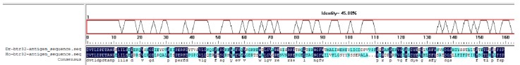
Author response image 2.
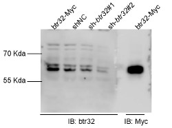
Reviewer #2 (Public review):
Weaknesses:
(1) Colocalization analyses (Figures 4G, 6I, 9D) require quantitative metrics (e.g., Pearson's coefficients) rather than representative images alone.
We concur with the reviewer's assessment. We have now performed quantitative colocalization analysis (Pearson's coefficients) for all indicated figures (4G, 6I, 9D). The quantitative results are now presented within the figures themselves and described in the revised figure legends.
(2) Figure 1 survival curves need annotated statistical tests (e.g., "Log-rank test, p=X.XX")
The survival curves have now been annotated with the specific p-values from the Log-rank (Mantel-Cox) test (see revised Figures 1A, 2E).
(3) Figure 2P GSEA should report exact FDR-adjusted *p*-values (not just "*p*<0.05").
Figure 2P (revised Figure S1J) has been updated to include the exact FDR p-values for the presented GSEA plots.
(4) Section 2 overextends on teleost sex-determination diversity, condensing to emphasize relevance to immune dimorphism would strengthen narrative cohesion.
The section on teleost sex-determination diversity in the Discussion (lines 357-365) has been condensed, with a more direct focus on how this diversity provides a unique context for studying immune dimorphism independent of canonical sex chromosomes, as exemplified by the zebrafish model.
(5) Limited discussion on whether this mechanism extends beyond Cyprinidae and its implications for teleost adaptation.
The discussion has been expanded (lines 375-386) to address the potential conservation of this mechanism. It is acknowledged that cyp17a2 is a teleost-specific gene, and it is hypothesized that its function in antiviral immunity may signify an adaptive innovation within this extensively diverse vertebrate group. It is suggested that further research in other teleost families will be essential to ascertain the broader evolutionary significance of the present findings.
Reviewer #2 (Recommendations for the authors):
(1) Expand the Discussion to address why teleosts may have evolved male-biased immunity. Consider: pathogen pressure differentials in aquatic vs. terrestrial environments; trade-offs between immune investment and reproductive strategies (e.g., male-male competition); comparative advantages in external fertilization systems.
We have expanded the discussion on lines 412-430, to address the potential conservation of this mechanism. We note that Cyp17a2 is a teleost-specific gene and speculate that its role in antiviral immunity represents an adaptive innovation within this highly diverse group of vertebrates. We propose that future studies of other teleost families are crucial for determining the broader evolutionary significance of our findings.
Reviewer #1 (Public review):
Summary:
This manuscript reports the discovery and characterization of the first bifunctional degrader of tankyrase. Notably, the tankyrase degrader exhibits stronger β-catenin inhibition and tumor growth suppression compared to conventional tankyrase inhibitors. Mechanistically, while tankyrase inhibitors stabilize tankyrase and promote Axin puncta formation - thereby impairing β-catenin degradation - the degrader avoids this effect, resulting in deeper suppression of β-catenin signaling. These findings suggest that targeted degradation of tankyrase offers a novel therapeutic strategy for β-catenin-driven cancers. Overall, this is a compelling study with significant translational potential.
Strengths:
(1) The manuscript presents a rigorous and well-executed study on a timely and impactful topic.
(2) The biochemical and cellular characterization of the tankyrase degrader is thorough, and the comparative analysis with tankyrase inhibitors is insightful.
(3) The finding that tankyrase stabilization by inhibitors may interfere with Axin function is novel and significant. It aligns with earlier observations (e.g., Huang 2009) that transient tankyrase overexpression can stabilize β-catenin independently of PAR domain activity.
(4) The use of TNKS1/2 knockout cells expressing catalytically inactive tankyrase to demonstrate β-catenin inhibitory activity of the tankyrase degrader is elegant.
(5) The finding that the tankyrase degrader has superior anti-proliferative effects in colorectal cancer models has important therapeutic implications.
Weaknesses:
(1) A key caveat is that the identified tankyrase degrader also targets GSPT1 for degradation. This raises the possibility that GSPT1 degradation may contribute to the observed β-catenin and tumor growth inhibition.
(2) The authors address this concern reasonably by showing that DLD1 cells resistant to GSPT1 degradation remain sensitive to the tankyrase degraded.
(3) To further strengthen this point, the authors might consider generating TNKS1/2 double knockout cells (e.g., in DLD1 or SW480 backgrounds) and demonstrating that the degrader loses its growth-inhibitory effect in these models. However, given the technical challenges of creating double knockouts in cancer cell lines, such experiments could be considered optional.
Reviewer #2 (Public review):
Summary:
The ADP-ribosyltransferase tankyrase controls many biological processes, many of which are relevant to human disease. This includes Wnt/beta-catenin signalling, which is dysregulated in many cancers, most notably colorectal cancer. Tankyrase is a positive regulator of Wnt/beta-catenin signalling in that it counters the activity of the beta-catenin destruction complex (DC). Catalytic inhibition of tankyrase not only blocks PAR-dependent ubiquitylation and degradation of AXIN1/2, the central scaffolding protein in the DC, but also tankyrase itself. As a result, blocking tankyrase gives rise to tankyrase accumulation, which may accentuate its non-catalytic functions, which have been proposed to drive Wnt/beta-catenin signalling. Most tankyrase catalytic inhibitors have shown limited efficacy and substantial toxicity in vivo. By developing tankyrase-directed PROTACs, the authors aim to block both catalytic and non-catalytic functions of tankyrase, aspiring to achieve a more complete inhibition of Wnt/beta-catenin signalling. The successfully developed PROTAC, based on the existing catalytic inhibitor IWR1, IWR1-POMA, induces the degradation of both TNKS and TNKS2, blocks beta-catenin-dependent transcription without stabilising the DC in puncta/degradasomes, and inhibits cancer cell growth in vitro. Mechanistically, this points to a scaffolding role of tankyrase in the DC, at least under conditions of tankyrase catalytic inhibition, in line with previous proposals.
Strengths:
The study clearly illustrates the incentive for developing a tankyrase degrader, namely, to abolish both catalytic and non-catalytic functions of tankyrase. By and large, the study achieves these ambitions, and the findings support the main conclusions, although the statement that a more complete inhibition of the pathway is achieved requires corroboration. The proteomics studies are powerful. IWR1-POMA constitutes a very useful tool to re-evaluate targeting of tankyrase in oncogenic Wnt/beta-catenin signalling. The paired compounds will benefit investigations of tankyrase scaffolding functions across many different biological systems controlled by tankyrase. The findings are exciting.
Weaknesses:
Although the results are promising and mostly compelling, the claim that the PROTACs provide "a deeper suppression of the WNT/β-catenin pathway activity" requires further corroboration, particularly at endogenous tankyrase levels.
There are also some other points that, if considered, would further improve the manuscript, as detailed below.
(1) Abstract and line 62: Many catalytic tankyrase inhibitors tend to display toxicity, which is likely on-target (e.g., 10.1177/0192623315621192; 10.1158/0008-5472). This constitutes the main limiting factor for these compounds. An incomplete inhibition of Wnt/beta-catenin signalling may contribute to the challenges, but this does not appear to be the dominant problem. A more prominent introduction to this important challenge is probably expected by the field.
(2) The authors do a good job in setting the scene for the need for tankyrase degraders. Their observations relating to the formation of puncta (degradasomes) being tankyrase-dependent are compatible with a previous study by Martino-Echarri et al. 2016 (10.1371/journal.pone.0150484): simultaneous silencing of TNKS and TNKS2 by RNAi abolishes degradasome formation. The paper is cited as reference 17, but only in passing, and deserves more prominence. (It includes an entire paragraph titled "Expression of tankyrases 1 and 2 is required for TNKSi-induced formation of axin puncta").
(3) Moreover, the scaffolding concept has been discussed comprehensively in other studies: 10.1111/bph.14038 and more recently 10.1042/BCJ20230230. There are also a few studies that focus on targeting the ankyrin repeat clusters of tankyrase to disengage substrates (10.1038/s41598-020-69229-y; 10.1038/s41598-019-55240-5) that illustrate the concept of blocking the scaffolding function. In that sense, the hypotheses are mature, and it is interesting to see some of them supported in this study. The authors could improve how they set their work into the context of these other efforts and proposals.
(4) In several places in the manuscript, the DC is referred to as "biomolecular condensate", at times even as a "classic example", implying that it operates through phase separation. This has not been demonstrated. In fact, super-resolution microscopy indicates that the puncta are not droplet-like (10.7554/eLife.08022), which would argue against the condensate hypothesis.
(5) It is beautiful to be able to use IWR1 and IWR1-POMA at identical concentrations for direct comparisons. However, this requires the two compounds to bind to tankyrase similarly well and reach the target to a comparable extent. How sure are authors that target engagement is comparable? Has this been evaluated?
(6) Figure 1F: It is not immediately apparent how IWR1-POMA shows more complete containment of Wnt/beta-catenin signalling. Most Wnt/beta-catenin targets lie close to the perfect diagonal, so I do not see how the statement "that IWR1-POMA controlled WNT/β-catenin signaling more effectively than IWR1" (in the legend of Figure 1F) is supported. Minimally, an expanded explanation would benefit the reader. Providing the colour-coding legend directly in the figure would help improve clarity. Also, the panel is very small and may benefit from a different presentation in the figure.
(7) Figure 2: The conclusion of a "deeper suppression" of signalling relies on overexpression of tankyrase in an otherwise tankyrase-null background. Have the authors attempted to measure reporter activity or endogenous gene expression without tankyrase overexpression, in Wnt3a-stimulated cells (in the context of a normal Wnt/beta-catenin pathway) or CRC cells at the basal level? Non-catalytic activity in a similar assay has previously been observed upon tankyrase overexpression (10.1016/j.molcel.2016.06.019). Whether or not there is a substantial scaffolding effect at endogenous tankyrase levels after tankyrase inhibition remains unconfirmed, and the PROTAC is a valuable tool to address this important question. The findings presented in Figure S7C and D go some way towards answering this question - these data could be presented more prominently, and similar assays could be performed in other cell systems.
(8) Line 237/238: "TNKS accumulation negatively impacts the catalytic activity of the DC (Figure 5D)" - the data do not show this. Beta-catenin levels are a surrogate readout for DC function (phosphorylation and ubiquitylation). Minimally, this requires rewording, with reference to beta-catenin levels.
(9) Line 303-304: Beta-catenin is thought to exchange at beta-catenin degradasomes; this is clear from previous FRAP assays and the observation that phospho-beta-catenin accumulates in degradasomes upon proteasome inhibition (10.1158/1541-7786.MCR-15-0125). However, degradasome size hasn't, to my knowledge, been related to activity. Can this be clarified, please?
(10) There are previous hypotheses/proposals that the sensitivity of CRC cells to tankyrase inhibition correlates with APC truncation or PIK3CA status (10.1158/1535-7163.MCT-16-0578; 10.1038/s41416-023-02484-8). Have the authors considered expanding their cell line panel (Figure S7) to sample a wider range of cell lines, including some that are wild-type with regard to APC or Wnt/beta-catenin signalling in general? This would be a valuable addition to the work. Quantitated colony formation data could be moved to the main body of the manuscript.
(11) The manuscript only mentions toxicity (i.e., therapeutic window) in the last sentence of the Discussion section. As this is THE main challenge with tankyrase inhibitors (as mentioned above), can the authors expand their discussion of this aspect? Is there an expectation that PROTACs may be less toxic?
(12) Figures 3, 4, 5A: For fluorescence microscopy experiments, can these be quantified, and can repeat data be included?
(13) Figure 4, S6: An additional channel illustrating the distribution of cells (e.g., nuclei, cytoskeleton, or membrane) would be helpful for orientation and context for the AXIN1 signal.
(14) How were cytosolic fractions of cells prepared to assess cytosolic beta-catenin levels? This detail is missing from the methods.
Reviewer #3 (Public review):
In this manuscript, Wang et al employ a chemical biology approach to investigate the differences between the enzymatic and scaffolding roles of tankyrase during Wnt β-catenin signalling. It was previously established that, in addition to its enzymatic activity, tankyrase 1/2 also plays a scaffolding function within the destruction complex, a property conferred by SAM-domain-dependent polymerization (PMID: 27494558). It is also known that TNKS1/2 is an autoregulated protein and that its enzymatic inhibition leads to accumulation of total TNKS proteins and stabilization of Axin punctae (through the scaffolding function of TNKS1/2), leading to rigidification of the DC and decreased β-catenin turnover. The authors surmised that this could, in part, explain the limited efficacy of TNKS1/2 catalytic inhibition for the treatment of colorectal cancers. To test this hypothesis, they evaluated a series of PROTAC molecules promoting the degradation of TNKS1/2 to block both the catalytic and scaffolding activities. They show that IWR1-POMA (their most active molecule) promotes more efficient suppression of beta-catenin-mediated transcription and is more active in inhibiting colorectal cancer cell and CRC patient-derived organoids growth. Mechanistically, the authors used FRAP to demonstrate that catalytic inhibitors of TNKS led to a reduced dynamic assembly of the DC (rigidification), whereas IWR1-POMA did not affect the dynamics.
Overall, this is an interesting study describing the design and development of a PROTAC for TNKS1/2 that could have increased efficacy where catalytic inhibitors have displayed limited activity. Knowing the importance of the scaffolding role of TNKS1/2 within the destruction complex, targeting both the catalytic and scaffolding roles certainly makes sense. The manuscript contains convincing evidence of the different mechanisms of the PROTAC vs catalytic inhibitors. Some additional efforts to quantify several of the experiments and to indicate the reproducibility and statistical analysis would strengthen the manuscript. Ultimately, it would have been great to evaluate the in vivo efficacy of IWR1-POMA in an in vivo CRC assay (APCmin mice or using PDX models); however, I realize that this is likely beyond the scope of this manuscript.
I have some recommendations listed below for consideration by the authors to strengthen their study:
(1) The title is slightly misleading, as it is already known that the scaffolding function of TNKS is important within the DC. The authors should consider incorporating the PROTAC targeting aspect in the title (e.g., PROTAC-mediated targeting of tankyrase leads to increased inhibition of betacat signaling and CRC growth inhibition).
(2) The authors should comment in the manuscript on the bell-shaped curve obtained with treatment of cells with the PROTACs (Figure S2C). This likely indicates tittering of the targets within a bifunctional molecule with increasing concentration (and likely reveals the auto-inhibition conferred by the catalytic inhibition alone).
(3) The authors comment that using G007-LK as warehead was unsuccessful, but they do not show data. Do the authors know why this was the case?
(4) Throughout the manuscript, the authors need to do a better job at quantifying their results (i.e., the western blots and the IF). For example, the degradation of TNKS1/2 in Figure 1D is not overly convincing. Similarly, the IF data in Figure 3 needs to be quantified in some ways. Along the same lines, the effect of IWR1-POMA treatments on the proliferation of cells and organoids should be quantified using viability assays... There is also no indication of how many times these experiments were performed and whether the blots shown are representative experiments. The quantification should include all experiments.
Author response:
Reviewer #1 (Public Review):
We thank the Reviewer for the favorable feedback. The major concern is the collateral degradation of GSPT1. As the Reviewer noted, IWR1-POMA was able to suppress colony formation in DLD-1 cells resistant to GSPT1/2 degrader, suggesting that TNKS but not GSPT degradation is responsible for growth inhibition.
We also appreciate that the Reviewer brought it to our attention an important early observation of the TNKS scaffolding effects. Cong reported in 2009 that overexpression of TNKS induced AXIN puncta formation in a SAM but not PARP domain-dependent manner (PMID 19759537). We will include this information in the revised manuscript.
Reviewer #2 (Public Review):
We thank the Reviewer for the encouraging and insightful comments. The major critique concerns whether TNKS degraders can suppress WNT/β-catenin signaling more effectively than TNKS inhibitors at endogenous TNKS levels. Fig. 1D shows that IWR1-POMA reduced the level of cytosolic β-catenin more effectively than IWR1 in Wnt3A-stimulated HEK293 cells without protein overexpression, and Fig. S7B shows that IWR1-POMA reduced STF signals more effectively than IWR1 in DLD-1 and SW480 cells with endogenous TNKS expression. We will corroborate these findings with additional cell lines during the revision.
(1) We agree with the Reviewer that on-target toxicities pose challenges to the development of WNT inhibitors. For example, LGK974 that inhibits PORCN to prevent the secretion of all WNT proteins showed significant on-target toxicity in human (PMC10020809), and G007-LK that inhibits TNKS to block canonical WNT signaling selectively exhibited weak efficacy and dose-limiting toxicity at 5‒30 mg/kg BID or 10‒60 mg/kg QD in various mouse xenograft models (PMID: 23539443). Similarly, G-631, another TNKS inhibitor, also showed dose-limiting toxicity without significant efficacy at 25‒100 mg/kg QD in mice (PMID: 26692561). However, G007-LK was well-tolerated at 200 mg/kg QD over 3 weeks in mice in another study (PMC5759193). Treating mice with G007-LK at 10 mg/kg QD over 6 months also improved glucose tolerance without notable toxicity (PMID 26631215). Importantly, constitutive silencing of both TNKS for 150 days in APC-null mice prevented tumorigenesis without damaging the intestines (PMC6774804). Furthermore, basroparib, a selective TNKS inhibitor, was well tolerated in a recent clinical trial (PMC12498271). We are therefore cautiously optimistic that TNKS degraders will have an improved therapeutic index compared with TNKS inhibitors.
(2) We agree with the Reviewer that Henderson's 2016 paper (PMC4773256) shed important light on the role of TNKS scaffolding in the DC. However, whereas this study demonstrated that knocking down both TNKS by siRNA prevented G007-LK to induce AXIN puncta, the function role of TNKS scaffolding in the DC remained unaddressed. We will include a more detailed description on Henderson's discovery.
(3) Indeed, Guettler demonstrated that TNKS scaffolding could promote WNT/β-catenin signaling in 2016, which forms the basis of the current work. Meanwhile, whereas there have been efforts to target the SAM or ARC domain to address TNKS scaffolding, our approach of targeting TNKS for degradation is complementary. We will provide a more detailed discussion of these studies.
(4) Biomolecular condensates are membrane less cellular compartments formed by phase separation of biomolecules, regardless of the physical/material properties (PMID: 28935776 and PMC7434221). Super-resolution microscopy studies by Peifer and Stenmark (PMC4568445 and PMID 26124443) showed that AXIN, APC, TNKS, and β-catenin interacted with each other to assemble into membraneless complexes, wherein AXIN and APC formed filaments throughout the DC. Peifer has also summarized evidence that supports the condensate nature of the DC (PMC6386181). However, we acknowledge that testing the physical properties of reconstituted DC (PMC8403986) will provide a better understanding of the nature, for example liquid vs. gel, of these condensates.
(5) We will evaluate the ability of IWR1 and IWR1-POMA to engage TNKS.
(6) We will modify Fig. 1F to improve clarity and readability.
(7) Fig. S7B shows that IWR1-POMA suppressed WNT/β-catenin signaling more effectively than IWR1 in APC-mut DLD-1 and SW480 CRC cells without TNKS overexpression. Similarly, Fig. S6B shows that IWR1-POMA provided a deeper suppression of STF signals in HeLa cells transfected with AXIN1 and β-catenin while expressing endogenous TNKS. These results provide evidence that inhibitor-induced TNKS scaffolding plays a significant role at endogenous TNKS expression levels. Separately, we will reorganize the figures to better present Fig. 7C and D as suggested by the Reviewer.
(8) We will rephrase "TNKS accumulation negatively impacts the catalytic activity of the DC".
(9) We apologize for confusing β-catenin phosphorylation with β-catenin abundance. Here, we refer the catalytic activity of the DC to as the ability of the DC to promote β-catenin degradation rather than the kinetics of β-catenin phosphorylation and ubiquitination. It is commonly observed that AXIN stabilization by TNKS inhibitors increases the DC size and reduces the β-catenin levels. Peifer has also noted that APC can increase the size and the "effective activity" of the DC (PMC5912785 and PMC4568445). As such, the induction of AXIN puncta by TNKS inhibitors is frequently used as an indicator of WNT/β-catenin pathway inhibition. However, because the DC only primes β-catenin but does not catalyze its degradation, we will revise our manuscript to improve accuracy and clarity.
(10) We will examine the effects of IWR1 and IWR1-POMA in additional cell lines, quantify the colony formation data, and reorganize the figures.
(11) As discussed above, evidence for on-target toxicity of WNT/β-catenin inhibition is mixed. Yet, the observation of no dose-limiting toxicity for basroparib at doses up to 360 mg QD in human (PMC12498271) is encouraging. PROTAC works by catalyzing target degradation, which is different from traditional catalytic inhibitors that require continuous target occupancy at a high level. Because IWR1-POMA has a durable effect on TNKS, we expect that a fully optimized TNKS degrader may allow less frequent dosing than basroparib and consequently an even more favorable therapeutic window.
(12/13) We will include quantification data, replicate information, and nuclei staining or cell outlines for the fluorescence microscopy experiments.
(14) Cytosolic fractions of cells were prepared using a commercial cytoplasmic extraction kit following manufacturer's instructions. We will include detailed information in the revised manuscript.
Reviewer #3 (Public Review):
We thank the Reviewer for the helpful suggestions.
(1) We will modify the title to include the PROTAC aspect.
(2) As the Reviewer suggested, the bell-shaped dose response of the PROTAC originated from the formation of saturated binary complexes. At high PROTAC concentrations, binding of TNKS and CRBN/VHL by separate PROTAC molecules impedes the formation of productive ternary complexes, which results in reduced degradation efficacy and consequently the hook effect.
(3) The structure-activity relationship of PROTACs is often unpredictable, as both the kinetics and thermodynamics of the target and E3 ligase binding play crucial roles. The lack of translation in degradation efficacy from IWR1 to G007-LK derived PROTACs may originate from differences in the binding kinetics or subtle changes in the orientation of the linker exit vector. We will include data on G007-LK in the revised manuscript.
(4) We will quantify the Western blots, immunofluorescence images, colony formation data, and the replicate information.
Author response:
Reviewer #1 (Public Review):
Summary:
The authors aim to demonstrate that GWAS summary statistics, previously considered safe for open sharing, can, under certain conditions, be used to recover individual-level genotypes when combined with large numbers of high-dimensional phenotypes. By reformulating the GWAS linear model as a system of linear programming constraints, they identify a critical phenotypeto-sample size ratio (R/N) above which genotype reconstruction becomes theoretically feasible.
Strengths:
There is conceptual originality and mathematical clarity. The authors establish a fundamental quantitative relationship between data dimensionality and privacy leakage and validate their theory through well-designed simulations and application to the GTEx dataset. The derivation is rigorous, the implementation reproducible, and the work provides a formal framework for assessing privacy risks in genomic research
We thank the reviewer for the positive assessment of our work’s conceptual originality, mathematical rigor, and reproducible implementation.
Weaknesses:
The study simplifies assumptions that phenotypes are independent, which is not the truth, and are measured without noise. Real-world data are highly correlated across different levels, not only genotype but also multi-omics, which may overstate recovery potential. The empirical evidence, while illustrative, is limited to small-scale data and idealized conditions; thus, the full practical impact remains to be demonstrated. GTEx analysis used only whole blood eQTL data from 369 individuals, which cannot capture the complexity, sample heterogeneity, or cross-tissue dependencies typical of biobank-scale studies
We recognize the concern regarding the independence and noiselessness assumptions in our frame work. While assuming independent, noiseless phenotypes represents an idealized scenario, it allows us to clearly demonstrate the conceptual potential of our framework. The GTEx whole blood analysis is intended as a proof-of-concept, illustrating feasibility rather than capturing full biological complexity. In the revised manuscript, we will clarify these assumptions, emphasize that practical reconstruction accuracy maybe lower in correlated and noisy real-world data, and expand empirical validation to multiple GTEx tissue sand independent cohorts to demonstrate robustness under more realistic conditions.
Reviewer #2 (PublicReview):
Summary:
This study focuses on the genomic privacy risks associated with Genome-Wide Association Study (GWAS) summary statistics, employing a three-tiered demonstration framework of” theoretical derivation- simulation experiments- real-data validation”. The research finds that when GWAS summary statistics are combined with high-dimensional phenotypic data, genotype recovery and individual re-identification can be achieved using linear programming methods. It further identifies key influencing factors such as the effective phenotype-to-sample sizeratio(R/N) and minor allele frequency(MAF). These findings provide practical reference for improving data governance policies in genomic research, holding certain real-world significance
Strengths:
This study integrates theoretical analysis, simulation validation, and the application of real world datasets to construct a comprehensive research framework, which is conducive to understanding and mitigating the risk of private information leakage in genomic research
We are glad the reviewer values our integration of theory, simulation, and real data
Weaknesses:
(1) Limited scope of variant types covered:
The analysis is conducted solely on Single Nucleotide Polymorphisms(SNPs), omitting other crucial genomic variant types such as Copy Number Variations(CNVs), Insertions/Deletions (InDels), and chromosomal translocations/inversions. From a genomic structure perspective, variants like CNVs and InDels are also core components of individual genetic characteristics, and in some disease-related studies, association signals for these variants can be even more significant than those for SNPs. From the perspective of privacy risk logic, the genotypes of these variants (e.g., copy number for CNVs, base insertion/deletion status for InDels) can also be quantified and could theoretically be inferred backwards using the combination of ”summary statistics +high-dimensional phenotypes”. Their privacy leakage risks might differ from those of SNPs(for instance, rare CNVs might be more easily re-identified due to higher genetic specificity)
This point raises an important clarification regarding variant types beyond SNPs. We would like to clarify that our mathematical framework is not inherently restricted to SNPs. In fact, it is broadly applicable to any genetic variant that can be represented numerically, e.g., allelic dosage (0/1/2), copy number counts for CNVs, or presence/absence indicators for InDels. Conceptually, CNVs , InDels, and other structural variants can be incorporated in the same way as SNPs.
The main limitation arises from the current availability of GWAS summary statistics for these non-SNP variant types (e.g., CNV dosages≥3), which are still relatively scarce. As a result, empirically evaluating our framework on these variant classes would be challenging. In the revision, we will explicitly emphasize the general applicability of our framework to diverse genetic variants while clearly noting this practical limitation. We also plan to include simulations to investigate the recovery accuracy associated with CNVs and InDels, which will further demonstrate the extensibility of our approach. It should be noted, however, that leaking genotypic data of ordinary SNPs already raises concerns, regardless of other types of genetic variants.
(2) Bias in data applicability scope:
Both the simulation experiments and real-data validation in the study primarily rely on European population samples (e.g.,489 Europe an samples from the 1000 Genomes Project; the genetic background of whole blood tissue samples from the GTEx project is not explicitly mentioned regarding non-European proportions). It only briefly notes a higher risk for African populations in the individual re-identification risk assessment, without conducting systematic analyses for other populations, such as East Asian, South Asian, or admixed American populations. Significant differences in genetic structure (e.g., MAF distribution, linkage disequilibrium patterns) exist across different populations. This may result in the R/N threshold and the relationship between MAF and recovery accuracy identified in the study not being fully applicable to other populations.
Hence, addressing the aforementioned issues through supplementary work would enhance the study’s scientific rigor and application value, potentially providing more comprehensive theoretical and technical support for” privacy protection” in genomic data sharing.
We acknowledge this valid concern regarding the generalizability of our findings. Our analysis already identifies MAF as a key factor influencing recovery accuracy, which begins to address population-specific genetic differences. Importantly, because our reconstruction method treats each variant independently, its success does not rely on population-specific LD patterns. The core determinant of feasibility is the ratio of phenotypic dimensions to sample size(R/N), a relationship we expect to hold a cross populations.
Nevertheless, we agree that further validation across diverse ancestries can be helpful. In the revised manuscript, we will try to include additional cohorts as extended validation analyses
Version 3 of this preprint has been peer-reviewed and recommended by Peer Community in Evolutionary Biology.<br /> See the peer reviews and the recommendation.
Version 3 of this preprint has been peer-reviewed and recommended by Peer Community in Evolutionary Biology.<br /> See the peer reviews and the recommendation.
Version 3 of this preprint has been peer-reviewed and recommended by Peer Community in Evolutionary Biology.<br /> See the peer reviews and the recommendation.
wdfy-3
DOI: 10.1093/genetics/iyae053
Resource: Caenorhabditis Genetics Center (RRID:SCR_007341)
Curator: @Apiekniewska
SciCrunch record: RRID:SCR_007341
RRID:CVCL_0532
DOI: 10.1155/humu/8719836
Resource: (CLS Cat# 300342/p657_SK-OV-3, RRID:CVCL_0532)
Curator: @scibot
SciCrunch record: RRID:CVCL_0532
RRID:SCR_020311
DOI: 10.1111/jnc.70295
Resource: Nanodrop Qubit 3 Fluorometer (RRID:SCR_020311)
Curator: @scibot
SciCrunch record: RRID:SCR_020311
RRID:SCR_022128
DOI: 10.1038/s41598-025-23545-3
Resource: Texas A and M University Microscopy and Imaging Center Core Facility (RRID:SCR_022128)
Curator: @scibot
SciCrunch record: RRID:SCR_022128
RRID:SCR_021737
DOI: 10.1038/s41467-025-64999-3
Resource: University of Ottawa Louise Pelletier Histology Core Facility (RRID:SCR_021737)
Curator: @scibot
SciCrunch record: RRID:SCR_021737
AB_2618166
DOI: 10.1038/s41467-025-64999-3
Resource: None
Curator: @scibot
SciCrunch record: RRID:AB_2618166
RRID:SCR_021845
DOI: 10.1038/s41467-025-64999-3
Resource: University of Ottawa Cell Biology and Image Acquisition Core Facility (RRID:SCR_021845)
Curator: @scibot
SciCrunch record: RRID:SCR_021845
RRID:SCR_021832
DOI: 10.1038/s41467-025-64999-3
Resource: University of Ottawa Preclinical Imaging Core Facility (RRID:SCR_021832)
Curator: @scibot
SciCrunch record: RRID:SCR_021832
RRID:SCR_012601
DOI: 10.1038/s41467-025-64999-3
Resource: Ottawa Hospital Research Institute StemCore Laboratories Core Facility (RRID:SCR_012601)
Curator: @scibot
SciCrunch record: RRID:SCR_012601
RRID:SCR_016202
DOI: 10.1007/s00125-025-06603-3
Resource: HIRN Human Pancreas Analysis Program (RRID:SCR_016202)
Curator: @scibot
SciCrunch record: RRID:SCR_016202
RRID:SCR_014387
DOI: 10.1007/s00125-025-06603-3
Resource: Integrated Islet Distribution Program (IIDP) (RRID:SCR_014387)
Curator: @scibot
SciCrunch record: RRID:SCR_014387
RRID:SCR_014393
DOI: 10.1007/s00125-025-06603-3
Resource: Human Islet Research Network (HIRN) (RRID:SCR_014393)
Curator: @scibot
SciCrunch record: RRID:SCR_014393
ipfs
https://bafybeid2rtfgfxlqdjo2nedenrk7miue5w6abimo7bz5k5gehglptsc32u.ipfs.dweb.link/?path=/♖/hyperpost/~/indyweb/📓/20/25/11/3
Weekly Log for 3rd week of October 2025 © indyweb
https://bafybeid2rtfgfxlqdjo2nedenrk7miue5w6abimo7bz5k5gehglptsc32u.ipfs.dweb.link/?path=/♖/hyperpost/~/indyweb/📓/20/25/11/3
Reviewer #3 (Public review):
Summary:
The manuscript by Shukla and colleagues presents a comprehensive study that addresses a central question in kinesin-1 regulation - how cargo binding to the kinesin light chain (KLC) tetratricopeptide repeat (TPR) domains triggers activation of full-length kinesin-1 (KHC). The authors combine AlphaFold3 modeling, biophysical analysis (fluorescence polarization, hydrogen-deuterium exchange), and electron microscopy to derive a mechanistic model in which the KLC-TPR domains dock onto coiled-coil 1 (CC1) of the KHC to form the "TPR shoulder," stabilizing the autoinhibited (λ-particle) conformation. Binding of a W/Y-acidic cargo motif (KinTag) or deletion of the CC1 docking site (TDS) dislocates this shoulder, liberating the motor domains and enhancing accessibility to cofactors such as MAP7. The results link cargo recognition to allosteric structural transitions and present a unified model of kinesin-1 activation.
Strengths:
(1) The study addresses a fundamental and long-standing question in kinesin-1 regulation using a multidisciplinary approach that combines structural modeling, quantitative biophysics, and electron microscopy.
(2) The mechanistic model linking cargo-induced dislocation of the TPR shoulder to activation of the motor complex is well supported by both structural and biochemical evidence.
(3) The authors employ elegant protein-engineering strategies (e.g., ElbowLock and ΔTDS constructs) that enable direct testing of model predictions, providing clear mechanistic insight rather than purely correlative data.
(4) The data are internally consistent and align well with previous studies on kinesin-1 regulation and MAP7-mediated activation, strengthening the overall conclusion.
Weaknesses:
(1) While the EM and HDX-MS analyses are informative, the conformational heterogeneity of the complex limits structural resolution, making some aspects of the model (e.g., stoichiometry or symmetry of TPR docking) indirect rather than directly visualized.
(2) The dynamics of KLC-TPR docking and undocking remain incompletely defined; it is unclear whether both TPR domains engage CC1 simultaneously or in an alternating fashion.
(3) The interplay between cargo adaptors and MAP7 is discussed but not experimentally explored, leaving open questions about the sequence and exclusivity of their interactions with CC1.
Reviewer #2 (Public review):
Summary:
In this study, the authors follow up on a previous suppressor screen of a temperature-sensitive allele of mis4 (mis4-G1487D), the cohesin loading factor in S. pombe, and identify additional suppressor alleles tied to the S. pombe TORC1 complex. Their analysis suggests that these suppressor mutations attenuate TORC1 activity, while enhanced TORC1 activity is deleterious in this context. Suppression of TORC1 activity also ameliorates chromosome segregation and spindle defects observed in the mis4-G1487D strain, although some more subtle effects are not reconstituted. The authors provide evidence that this genetic suppression is also tied to the reconstitution of cohesin loading. Moreover, disrupting TORC1 also enhances Mis4/cohesin association with chromatin (likely reflecting enhanced loading) in WT cells, while rapamycin treatment can enhance the robustness of chromosome transmission. These effects likely arise directly through TORC1 or its downstream effector kinases, as TORC1 co-purifies with Mis4 and Rad21; these factors are also phosphorylated in a TORC1-dependent fashion. Disrupting Sck2, a kinase downstream of TORC1, also suppresses the mis4-G1487D allele while simultaneous disruption of Sck1 and Sck2 enhances cohesin association with chromatin, albeit with differing effects on phosphorylation of Mis4 and Psm1/Scm1. Phosphomutants of Mis4 and Psm1 that mimic observed phosphorylation states identified by mass spectrometry that are TORC1-dependent also suppressed phenotypes observed in the mis4-G1487D background. Last, the authors provide evidence that the mis4-G1487D background and TORC1 mutant backgrounds display an overlap in the dysregulation of genes that respond to environmental conditions, particularly in genes tied to meiosis or other "stress".
Overall, the authors provide compelling evidence from genetics, biochemistry, and cell biology to support a previously unknown mechanism by which nutrient sensing regulates cohesin loading with implications for the stress response. The technical approaches are generally sound, well-controlled, and comprehensive.
Specific Points:
(1) While the authors favor the model that the enhanced cohesin loading upon diminished TORC1 activity helps cells to survive harsh environmental conditions, as starvation of S. pombe also drives commitment to meiosis, it seems as plausible that enhanced cohesin loading is related to preparing the chromosomes to mate.
(2) Related to Point 1, the lab of Sophie Martin previously published that phosphorylation of Mis4 characterizes a cluster of phosphotargets during starvation/meiotic induction (PMID: 39705284). This work should be cited, and the authors should interrogate how their observations do or do not relate to these prior observations (are these the same phosphosites?).
(3) It would be useful for the authors to combine their experimental data sets to interrogate whether there is a relationship between the regions where gene expression is altered in the mis4-G1487D strain and changes in the loading of cohesin in their ChIP experiments.
(4) Given that the genes that are affected are predominantly sub-telomeric while most genes are not affected in the mis4-G1487D strain, one possibility that the authors may wish to consider is that the regions that become dysregulated are tied to heterochromatic regions where Swi6/HP1 has been implicated in cohesin loading.
(5) It would be helpful to show individual data points from replicates in the bar graphs - it is not always clear what comprises the data sets, and superplots would be of great help.
Reviewer #1 (Public review):
Summary:
The authors investigate how UVC-induced DNA damage alters the interaction between the mitochondrial transcription factor TFAM and mtDNA. Using live-cell imaging, qPCR, atomic force microscopy (AFM), fluorescence anisotropy, and high-throughput DNA-chip assays, they show that UVC irradiation reduces TFAM sequence specificity and increases mtDNA compaction without protecting mtDNA from lesion formation. From these findings, the authors suggest that TFAM acts as a "sensor" of damage rather than a protective or repair-promoting factor.
Strengths:
(1) The focus on UVC damage offers a clean system to study mtDNA damage sensing independently of more commonly studied repair pathways, such as oxidative DNA damage. The impact of UVC damage is not well understood in the mitochondria, and this study fills that gap in knowledge.
(2) In particular, the custom mitochondrial genome DNA chip provides high-resolution mapping of TFAM binding and reveals a global loss of sequence specificity following UVC exposure.
(3) The combination of in vitro TFAM DNA biophysical approaches, combined with cellular responses (gene expression, mtDNA turnover), provides a coherent multi-scale view.
(4) The authors demonstrate that TFAM-induced compaction does not protect mtDNA from UVC lesions, an important contribution given assumptions about TFAM providing protection.
Weaknesses:
(1) The authors show a decrease in mtDNA levels and increased lysosomal colocalization but do not define the pathway responsible for degradation. Distinguishing between replication dilution, mitophagy, or targeted degradation would strengthen the interpretation
(2) The sudden induction of mtDNA replication genes and transcription at 24 h suggests that intermediate timepoints (e.g., 12 hours) could clarify the kinetics of the response and avoid the impression that the sampling coincidentally captured the peak.
(3) The authors report no loss of mitochondrial membrane potential, but this single measure is limited. Complementary assays such as Seahorse analysis, ATP quantification, or reactive oxygen species measurement could more fully assess functional integrity.
(4) The manuscript briefly notes enrichment of TFAM at certain regions of the mitochondrial genome but provides little interpretation of why these regions are favored. Discussion of whether high-occupancy sites correspond to regulatory or structural elements would add valuable context.
(5) It remains unclear whether the altered DNA topology promotes TFAM compaction or vice versa. Addressing this directionality, perhaps by including UVC-only controls for plasmid conformation, would help disentangle these effects if UVC is causing compaction alone.
(6) The authors provide a discrepancy between the anisotropy and binding array results. The reason for this is not clear, and one wonders if an orthogonal approach for the binding experiments would elucidate this difference (minor point).
Assessment of conclusions:
The manuscript successfully meets its primary goal of testing whether TFAM protects mtDNA from UVC damage and the impact this has on the mtDNA. While their data points to an intriguing model that TFAM acts as a sensor of damaged mtDNA, the validation of this model requires further investigation to make the model more convincing. This is likely warranted for a follow-up study. Also, the biological impact of this compaction, such as altering transcription levels, is not clear in this study.
Impact and utility of the methods:
This work advances our understanding of how mitochondria manage UVC genome damage and proposes a structural mechanism for damage "sensing" independent of canonical repair. The methodology, including the custom TFAM DNA chip, will be broadly useful to the scientific community.
Context:
The study supports a model in which mitochondrial genome integrity is maintained not only by repair factors, but also by selective sequestration or removal of damaged genomes. The demonstration that TFAM compaction correlates with damage rather than protection reframes an interesting role in mtDNA quality control.
Reviewer #2 (Public review):
Summary:
King et al. present several sets of experiments aimed to address the potential impact of UV irradiation on human mitochondrial DNA as well as the possible role of mitochondrial TFAM protein in handling UV-irradiated mitochondrial genomes. The carefully worded conclusion derived from the results of experiments performed with human HeLa cells, in vitro small plasmid DNA, with PCR-generated human mitochondrial DNA, and with UV-irradiated small oligonucleotides is presented in the title of the manuscript: "UV irradiation alters TFAM binding to mitochondrial DNA". The authors also interpret results of somewhat unconnected experimental approaches to speculate that "TFAM is a potential DNA damage sensing protein in that it promotes UVC-dependent conformational changes in the [mitochondrial] nucleoids, making them more compact." They further propose that such a proposed compaction triggers the removal of UV-damaged mitochondrial genomes as well as facilitates replication of undamaged mitochondrial genomes.
Strengths:
(1) The authors presented convincing evidence that a very high dose (1500 J/m2) of UVC applied to oligonucleotides covering the entire mitochondrial DNA genome alleviates sequence specificity of TFAM binding (Figure 3). This high dose was sufficient to cause UV lesions in a large fraction of individual oligonucleotides. The method was developed in the lab of one of the corresponding authors (reference 74) and is technically well-refined. This result can be published as is or in combination with other data.
(2) The manuscript also presents AFM evidence (Figure 4) that TFAM, which was long known to facilitate compaction of the mitochondrial genome (Alam et al., 2003; PMID 12626705 and follow-up citations), causes in vitro compaction of a small pUC19 plasmid and that approximately 3 UVC lesions per plasmid molecule result in a slight, albeit detectable, increase in TFAM compaction of the plasmid. Both results can be discussed in line with a possible extrapolation to in vivo phenomena, but such a discussion should include a clear statement that no in vivo support was provided within the set of experiments presented in the manuscript.
Weaknesses:
Besides the experiments presented in Figures 3 and 4, other results do not either support or contradict the speculation that TFAM can play a protective role, eliminating mitochondrial genomes with bulky lesions by way of excessive compaction and removing damaged genomes from the in vivo pool.
To specify these weaknesses:
(1) Figure 1 - presents evidence that UVC causes a reduction in the number of mitochondrial spots in cells. The role of TFAM is not assessed.
(2) Figure 2 - presents evidence that UVC causes lesions in mitochondrial genomes in vivo, detectable by qPCR. No direct assessment of TFAM roles in damage repair or mitochondrial DNA turnover is assessed despite the statements in the title of Figure 2 or in associated text. Approximately 2-fold change in gene expression of TFAM and of the three other genes does not provide any reasonable support to suggestion about increased mitochondrial DNA turnover over multiple explanations on related to mitochondrial DNA maintenance.
(3) Figure 5. Shows that TFAM does not protect either mitochondrial nucleoids formed in vitro or mitochondrial DNA in vivo from UVC lesions as well as has no effect on in vivo repair of UV lesions.
(4) Figure 6: Based on the above analysis, the model of the role of TFAM in sensing mtDNA damage and elimination of damaged genomes in vivo appears unsupported.
(5) Additional concern about Figure 3 and relevant discussion: It is not clear if more uniform TFAM binding to UV irradiated oligonucleotides with varying sequence as compared to non-irradiated oligonucleotides can be explained by just overall reduced binding eliminating sequence specific peaks.
Reviewer #3 (Public review):
Summary:
The study is grounded in the observations that mitochondrial DNA (mtDNA) exhibits a degree of resistance to mutagenesis under genotoxic stress. The manuscript focuses on the effects of UVC-induced DNA damage on TFAM-DNA binding in vitro and in cells. The authors demonstrate increased TFAM-DNA compaction following UVC irradiation in vitro based on high-throughput protein-DNA binding and atomic force microscopy (AFM) experiments. They did not observe a similar trend in fluorescence polarization assays. In cells, the authors found that UVC exposure upregulated TFAM, POLG, and POLRMT mRNA levels without affecting the mitochondrial membrane potential. Overexpressing TFAM in cells or varying TFAM concentration in reconstituted nucleoids did not alter the accumulation or disappearance of mtDNA damage. Based on their data, the authors proposed a plausible model that, following UVC-induced DNA damage, TFAM facilitates nucleoid compaction, which may serve to signal damage in the mitochondrial genome.
Strengths:
The presented data are solid, technically rigorous, and consistent with established literature findings. The experiments are well-executed, providing reliable evidence on the change of TFAM-DNA interactions following UVC irradiation. The proposed model may inspire future follow-up studies to further study the role of TFAM in sensing UVC-induced damage.
Weaknesses:
The manuscript could be further improved by refining specific interpretations and ensuring terminology aligns precisely with the data presented.
(1) In line 322, the claim of increased "nucleoid compaction" in cells should be removed, as there is a lack of direct cellular evidence. Given that non-DNA-bound TFAM is subject to protease digestion, it is uncertain to what extent the overexpressed TFAM actually integrates into and compacts mitochondrial nucleoids in the absence of supporting immunofluorescence data.
(2) In lines 405 and 406, the authors should avoid equating TFAM overexpression with compaction in the cellular context unless the compaction is directly visualized or measured.
(3) In lines 304 and 305 (and several other places throughout the manuscript), the authors use the term "removal rates". A "removal rate" requires a direct comparison of accumulated lesion levels over a time course under different conditions. Given the complexity of UV-induced DNA damage-which involves both damage formation and potential removal via multiple pathways-a more accurate term that reflects the net result of these opposing processes is "accumulated DNA damage levels." This terminology better reflects the final state measured and avoids implying a single, active 'removal' pathway without sufficient kinetic data.
(4) In line 357, the authors refer to the decrease in the total DNA damage level as "The removal of damaged mtDNA". The decrease may be simply due to the turnover and resynthesis of non-damaged mtDNA molecules. The term "removal" may mislead the casual reader into interpreting the effect as an active repair/removal process.
Reviewer #2 (Public review):
Summary:
In this manuscript, the authors combined coarse-grained structure-based model simulation, optical tweezer experiments, and AI-based analysis to assess the knotting behavior of the TrmD-Tm1570 protein. Interestingly, they found that while the structure-based model can fold the single knot from TrmD and Tm1570, the double-knot protein TrmD-Tm1570 cannot form a knot itself, suggesting the need for chaperone proteins to facilitate this knotting process. This study has strong potential to understand the molecular mechanism of knotted proteins, supported by many experimental and simulation evidence. However, there are a few places that appear to lack sufficient details, and more clarification in the presentation is needed.
Strengths:
A combination of both experimental and computational studies.
Weaknesses:
There is a lack of detail to support some statements.
(1) The use of the AI-based method, SOM, can be emphasized further, especially in its analysis of the simulated unfolding trajectories and discovery of the four unfolding/folding pathways. This will strengthen the statistical robustness of the discovery.
(2) The manuscript would benefit from a clearer description of the correlation between the simulation and experimental results. The current correlation, presented in the paragraph starting from Line 250, focuses on measured distances. The authors could consider providing additional evidence on the order of events observed experimentally and computationally. More statistical analyses on the experimental curves presented in Figure 4 supplement would be helpful.
(3) How did the authors calibrate the timescale between simulation and experiment? Specifically, what is the value \tau used in Line 270, and how was it calculated? Relevant information would strengthen the connection between simulation and experiment.
(4) In Line 342, the authors comment that whether using native contacts or not, they cannot fold double-knotted TrmD-Tm1570. Could the authors provide more details on how non-native interactions were analyzed?
(5) It appears that the manuscript lacks simulation or experimental evidence to support the statement at Line 343: While each domain can self-tie into its native knot, this process inhibits the knotting of the other domain. Specifically, more clarification on this inhibition is needed.
Author response:
The following is the authors’ response to the original reviews.
Reviewer #1 (Public review):
Summary:
The researchers sought to determine whether Ptbp1, an RNA-binding protein formerly thought to be a master regulator of neuronal differentiation, is required for retinal neurogenesis and cell fate specification. They used a conditional knockout mouse line to remove Ptbp1 in retinal progenitors and analyzed the results using bulk RNA-seq, single-cell RNA-seq, immunohistochemistry, and EdU labeling. Their findings show that Ptbp1 deletion has no effect on retinal development, since no defects were found in retinal lamination, progenitor proliferation, or cell type composition. Although bulk RNA-seq indicated changes in RNA splicing and increased expression of late-stage progenitor and photoreceptor genes in the mutants, and single-cell RNA-seq detected relatively minor transcriptional shifts in Müller glia, the overall phenotypic impact was low. As a result, the authors conclude that Ptbp1 is not required for retinal neurogenesis and development, thus contradicting prior statements about its important role as a master regulator of neurogenesis. They argue for a reassessment of this stated role. While the findings are strong in the setting of the retina, the larger implications for other areas of the CNS require more investigation. Furthermore, questions about potential reimbursement from Ptbp2 warrant further research.
Strengths:
This study calls into doubt the commonly held belief that Ptbp1 is a critical regulator of neurogenesis in the CNS, particularly in retinal development. The adoption of a conditional knockout mouse model provides a reliable way for eliminating Ptbp1 in retinal progenitors while avoiding the off-target effects often reported in RNAi experiments. The combination of bulk RNA-seq, scRNA-seq, and immunohistochemistry enables a thorough examination of molecular and cellular alterations at both embryonic and postnatal stages, which strengthens the study's findings. Furthermore, using publicly available RNA-Seq datasets for comparison improves the investigation of splicing and expression across tissues and cell types. The work is wellorganized, with informative figure legends and supplemental data that clearly show no substantial phenotypic changes in retinal lamination, proliferation, or cell destiny, despite identified transcriptional and splicing modifications.
We thank the Reviewer for their evaluation of the strengths of the study.
Weaknesses:
The retina-specific method raises questions regarding whether Ptbp1 is required in other CNS locations where its neurogenic roles were first proposed. The claim that Ptbp1 is "fully dispensable" for retinal development may be toned down, given the transcriptional and splicing modifications identified. The possibility of subtle or transitory impacts, such as ectopic neuron development followed by cell death, is postulated, but not completely investigated. Furthermore, as the authors point out, the compensating potential of increased Ptbp2 warrants additional exploration. Although the study performs well in transcriptome and histological analyses, it lacks functional assessments (such as electrophysiological or behavioral testing) to determine if small changes in splicing or gene expression affect retinal function. While 864 splicing events have been found, the functional significance of these alterations, notably the 7% that are neuronalenriched and the 35% that are rod-specific, has not been thoroughly investigated. The manuscript might be improved by describing how these splicing changes affect retinal development or function.
We have revised the text to address these points as requested.
Reviewer #2 (Public review):
Summary:
Ptbp1 has been proposed as a key regulator of neuronal fate through its role in repressing neurogenesis. In this study, the authors conditionally inactivated Ptbp1 in mouse retinal progenitor cells using the Chx10-Cre line. While RNA-seq analysis at E16 revealed some changes in gene expression, there were no significant alterations in retinal cell type composition, and only modest transcriptional changes in the mature retina, as assessed by immunofluorescence and scRNAseq. Based on these findings, the authors conclude that Ptbp1 is not essential for cell fate determination during retinal development.
Strengths:
Despite some effects of Ptbp1 inactivation (initiated around E11.5 with the onset of Chx10-Cre activity) on gene expression and splicing, the data convincingly demonstrate that retinal cell type composition remains largely unaffected. This study is highly significant since it challenges the prevailing view of Ptbp1 as a central repressor of neurogenesis and highlights the need to further investigate, or re-evaluate, its role in other model systems and regions of the CNS.
We thank the Reviewer for their evaluation of the strengths of the study.
Weaknesses:
A limitation of the study is the use of the Chx10-Cre driver, which initiates recombination around E11. This timing does not permit assessment of Ptbp1 function during the earliest phases of retinal development, if expressed at that time.
We have revised the text to address the potential limitations of the use of the Chx10-Cre driver in this study.
Reviewer #1 (Recommendations for the authors):
(1) The author only selected scRNA-Seq datasets to examine the expression patterns of Ptbp1 in the retina; incorporating immunostaining analysis in the mouse retina is necessary.
Ptbp1 expression patterns in the mouse retina were performed in Fig. 1b-1d, where Ptbp1 expression was analyzed via immunostaining for Ptbp1 protein in Chx10-Cre control and Ptbp1KO retinas at E14, P1, and P30, and are quantified in Fig. 1e.
(2) In Figure 1, Ptbp1 signals were still detected in the KO mice, with the author suggesting that this may indicate cross-reactivity with an unknown epitope. Why is this unknown epitope only detected in the ganglion cell layer? Additional antibodies are needed to confirm the staining results. Furthermore, it is essential to verify the KO at the mRNA level using PCR.
We are unsure of the identity of this cross-reacting epitope, although it might be Ptbp2, which is enriched expressed in immature retinal ganglion cells (Fig. S1). In any case, we do not believe that the identity of this epitope is not relevant to assessing the efficiency of Ptbp1 deletion, as it is not detectably expressed in retinal ganglion cells in any case (Fig. S1).
Although the heatmap in Figure 2B indicates a decrease in Ptbp1 levels in the KO mice, the absence of statistical data makes it difficult to evaluate the KO efficiency.
Respectfully, we believe that Ptbp1 knockout efficiency is adequately addressed using immunohistochemistry, and that further statistical analysis is not essential here.
Cre staining of the Chx10-Cre;Ptbp1lox/lox mice or using reporter lines is also suggested to indicate the theoretically knockout cells. Providing high-power images of the Ptbp1 staining would help readers clearly recognize the staining signals.
To clarify the identity of the knockout cells, we have updated Figure 1 to include the Chx10-CreEGFP staining which more clearly delineates the cells in which Ptbp1 is deleted. Regarding verification of the knockout, we believe additional PCR assays are not necessary, as we have already demonstrated efficient loss of Ptbp1 in Chx10-Cre-expressing cells at the RNA level by both single-cell RNA-sequencing and bulk RNA-sequencing, and also at the protein level by immunohistochemistry. Sun1-GFP Cre reporter lines are also used in Figures 1 and S2 to visualize patterns of Cre activity, a point which is now highlighted in the text. Together, these approaches provide sufficient evidence for effective Ptbp1 knockout.
(3) The possibility of ectopic neuron formation followed by cell death is intriguing but underexplored. Consider adding apoptosis assays (e.g., TUNEL staining) at early developmental stages to test this hypothesis.
While apoptosis assays such as TUNEL staining would be helpful to address this hypothesis, we feel incorporating these additional experiments is currently beyond the scope of this study. We agree the possibility of cell death is intriguing and plan to explore this in future work.
(4) On page 4, the statement "We did not observe any significant differences ... Chx10Cre;Ptbp1lox/lox mice (Fig. 2b,c)" should refer to Fig. 3b,c instead.
We have changed the text to refer to Fig. 3b,c.
(5) The labeling in Figure 3 as "Cre-Ptbp1" is inconsistent with the figure legend "Ptbp1-Ctrl.".
This language was used because the samples for EdU staining in Figure 3 were Chx10-Cre negative Ptbp1<sup>lox/lox</sup> mice. We have updated the language in the manuscript and figure to reflect the genotypes more clearly.
(6) P30 mice are still sexually immature; the term "adolescent" or "juvenile" should be used instead of "adult."
We have updated the language in the text from “adult” to “adolescent” to describe P30 mice, although the retina itself is mature by this age.
Reviewer #2 (Recommendations for the authors):
(1) As mentioned in the public review, a limitation of the study is that Ptbp1 KO is not induced prior to E11. The authors should acknowledge this limitation and include in the Discussion that the use of the Chx10-Cre line does not permit evaluation of a potential role for Ptbp1 during very early stages of retinal development, should it be expressed at that time (an aspect that would be important to determine).
We and have added this limitation to the Discussion in the sentence highlighted below.
Furthermore, the use of the Chx10-Cre transgene in this study does not exclude a potential role for Ptbp1 during very early stages of retinal development prior to E11 (pg. 6).
(2) While the data convincingly show no significant changes in retinal cell type distribution in Ptbp1 mutants, the claims in the abstract and introduction that Ptbp1 is "dispensable for retinal development" or "dispensable for the process of neurogenesis" may be overstated. Indeed, the results indicate that loss of Ptbp1 function influences retinal development by promoting neurogenesis through induction of a neuronal-like splicing program in neural progenitors. Concluding solely that Ptbp1 is dispensable for retinal cell fate specification, rather than for retinal development as a whole, would thus seem more accurate.
We have updated the language in the text to reflect Ptbp1’s role in regulating retinal cell fate specification more clearly.
(3) The authors conclude from Figure 5 that "No changes in the identity or composition of any retinal cell type were observed." Which statistical test was applied to support this conclusion? The figure indicates that Müller cells comprise 10.5% of the total cell population in controls versus 8.2% in Ptbp1-KO retinas. It may be important to consider the overall distribution of glia versus all neurons (rather than each neuron subtype individually). While the observed difference (~2% more glia at the expense of neurons) appears modest, it would be important to determine whether this trend is consistent and statistically significant.
To evaluate cell type composition, we performed differential expression analysis across all major retinal cell types and compared proportional cell type representation between control and Ptbp1 KO retinas. While these analyses did not reveal marked differences in any specific cell type, we acknowledge that the scRNA-Seq dataset includes a single experimental replicate, containing two retinas in each replicate. Therefore, we cannot draw firm statistical conclusions regarding the relative distribution of glia versus neurons, and the modest difference observed in glia cell proportion should be interpreted with caution. We agree that assessing glia-to-neuron ratios across additional replicates will be important in future studies.
(4) Referringx to Figure S1 (scRNA-seq data), the authors state that Ptbp1 mRNA is robustly expressed in retinal progenitors and Müller glia in both mouse and human retina. While the immunostaining in Figure 4 indeed clearly shows strong expression in Müller cells, the scRNAseq data presented in Figure S1 do not support the claim of "robust" expression in Müller glia in the mouse retina. This is even more striking in the human data, where panels F and H show that Ptbp1 is expressed at extremely low, certainly not "robust", levels in Müller cells. The corresponding sentence in the Results section should therefore be revised to more accurately reflect the data presented in Figure S1, or be supported by complementary immunofluorescence evidence.
We thank the reviewer for this comment. We have revised this section of the Results to better reflect Fig S1, as follows:
We observe high expression levels of Ptbp1 mRNA in primary retinal progenitors in both species and Müller glia in mouse retina, with weaker expression in neurogenic progenitors, and little expression detectable in neurons at any developmental age.
(5) When mentioning potential compensation by Ptbp2, the authors may also consider discussing the possibility that compensatory mechanisms can differ between knockdown and knockout approaches. In this context, it is noteworthy that a recent study by Konar et al., Exp Eye Res, 2025 (published after the submission of the present manuscript) reports that Ptbp1 knockdown promotes Müller glia proliferation in zebrafish.
We thank the reviewer for this suggestion. To address this, we have included a section considering this possibility in the discussion section highlighted below.
It is also possible that compensatory mechanisms differ between knockdown and knockout approaches. Notably, a recent study (Konar et al. 2025) reported that Ptbp1 knockdown promotes Müller glia proliferation in zebrafish, suggesting that effects of acute reduction of Ptbp1 may not fully mirror those of complete loss-of-function.
(6) The statistical analyses were performed using a t-test. However, this parametric test is not appropriate for experiments with low sample sizes. A non-parametric test, such as the MannWhitney test, would be more suitable in this context. Furthermore, performing statistical analysis on n = 2 (Figure 3C) is not statistically valid.
We thank the reviewer for this comment. We agree that with a small n, non-parametric tests are more appropriate. We have added additional retinas (now n=5) for the Ptbp1-KO condition in Figure 3C and reanalyzed with the appropriate non-parametric Mann-Whitney test. For all other datasets with sufficient replicates (n≥ 4/genotype), parametric tests such as unpaired t-tests remain valid, and the results are consistent with non-parametric testing.
(7) Figure S3 is accompanied by only a brief explanation in the Results section (a single sentence despite the figure containing six panels), which makes it difficult for readers unfamiliar with this type of data to interpret.
We thank the reviewer for the suggestion. To address this, we have included a more detailed explanation of Supplementary Figure S3 to better clarify our analysis of mature neuronal and glial cell types in both Ptbp1-deficient and wild-type animals. The relevant text now reads:
Notably, splicing patterns in Ptbp1-deficient retinas showed stronger correlation with Thy1positive neurons— which exhibit low Ptbp1 expression—and minimal overlap with microglia and auditory hair cells, the adult cell types with the highest Ptbp1 levels (Fig. S3).
Gene expression and splicing changes were compared across several reference tissues: heart tissue and Thy1-positive neurons, mature hair cells, microglia, and astrocytes (Fig. S3a,b). A heatmap of differentially expressed genes showed that while Ptbp1-deficient retinas diverged from WT retinas, their expression profiles did not resemble those of fully differentiated cell types like rods, astrocytes, or adult WT retina (Fig. S3c). Consistently, Pearson correlation analysis revealed that Ptbp1-deficient and WT retinas were more similar to each other than to fully differentiated neuronal or glial populations (Fig. S3d). Splicing profile analysis further revealed that while there was high correlation of PSI between Ptbp1-deficient and WT retinas, Ptbp1deficient retinas more closely resembled Thy1-positive neurons, whereas WT retinas aligned more strongly with mature cells such as astrocytes, microglia, and auditory hair cells (Fig. S3ef). Together, these results suggest that although Ptbp1 loss induces hundreds of alternative splicing events, the magnitude of PSI changes in the KO retinas remains considerably lower than that seen in fully differentiated cell types (Extended Data 3). Thus, while a subset of splicing events overlaps with those characteristic of mature neurons or rods, the overall splicing and expression profiles of KO retinas are more similar to those of developing retinal tissue rather than terminally differentiated neuronal or glial populations.
(8) To assess progenitor proliferation, the authors performed EdU labeling experiments in P0 retinas. Is there a rationale for not examining earlier developmental time points to evaluate potential effects on early RPCs?
We thank the reviewer for this comment. We chose to perform EdU labeling experiments at P0 for several reasons. P0 represents a developmental stage where RPCs are actively proliferating and represent ~35% of all retina cells, and the retina is transitioning to intermediate-late-stage development, providing sufficient time to ensure efficient and widespread disruption of Ptbp1. Earlier embryonic timepoints were not examined here, as addressing all stages of development was beyond the scope of this current study. However, we agree that investigating whether Ptbp1 plays stage-specific roles during development on early RPCs is an important question and potential future direction.
(9) In Figure S2, panel D shows staining in GCL under the Ptbp1 condition that does not make sense and is inconsistent with panel C. If possible, the authors should provide an alternative image to prevent any confusion.
Thank you for bringing this to our attention. The image shown for Ptbp1-KO in Figure 2d shows Sun1-eGFP labeling, which labels every cell affected by the Cre condition. The genotype for this mouse was Chx10-Cre;Ptbp1lox/lox;Sun1-GFP. We apologize for any confusion and have updated the genotype in the figure legend.
(10) The authors should revise the following sentence at the end of the Discussion section, as its meaning is unclear: "...and conditions for in vitro analysis may have accurately replicated conditions in the native CNS."
We thank the reviewer for this comment and have revised this sentence in the discussion for the sentence below.
Previous studies using knockdown may have been complicated by off-target effects (Jackson et al. 2003), and conditions for in vitro analysis may not have accurately replicated conditions in the native CNS.
[p31] Kate Starbird, Ahmer Arif, and Tom Wilson. Disinformation as Collaborative Work: Surfacing the Participatory Nature of Strategic Information Operations. Proc. ACM Hum.-Comput. Interact., 3(CSCW):127:1–127:26, November 2019. URL: https://dl.acm.org/doi/10.1145/3359229 (visited on 2023-12-08), doi:10.1145/3359229.
For the bibliography, I was really interested in [p31], “Disinformation as Collaborative Work: Surfacing the Participatory Nature of Strategic Information Operations.” Just from the title and description, it already changes how I think about fake news. Before, I imagined disinformation like one bad actor or one troll farm pushing lies. This paper instead frames it as a kind of “collaborative work,” where many different people and tools are involved, sometimes even regular users who don’t realize they are part of the campaign. That idea is kind of scary, because it means disinformation is not only top-down, but also bottom-up and participatory. It also connects nicely with the chapter’s point that crowdsourcing can be used both for good (like Foldit or crisis help) and for harmful goals. It makes me feel we really need better education on how to not accidentally help spread these operations.
books and scholarly articles. Academic books generally fall into three categories: (1) textbooks written with students in mind, (2) monographs which give an extended report on a large research project, and (3) edited-volumes in which each chapter is authored by different people. Scholarly articles appear in academic journals, which are published multiple times a year in order to share the latest research findings with scholars in the field.
this is what you should look at for your research
Remembering: Recalling basic facts and concepts.记忆 :回忆基本事实和概念。 Understanding: Explaining ideas or processes.理解 :解释概念或过程。 Applying: Using knowledge in new situations.应用 :将知识运用到新的情境中。 Analyzing: Breaking down information into components.分析 :将信息分解成各个组成部分。 Evaluating: Making judgments based on criteria and standards.评价 :根据标准和准则做出判断。 Creating: Producing original work or solutions.创造 :产生原创作品或解决方案。
布鲁姆分类法 1. 记忆: 回忆基本事实和概念 2. 理解: 解释概念或者过程 3. 应用: 将只是运用到新的情境中 4. 分析: 将信息分级成各个组成部分 5. 评价: 根据标准和准则做出判断 6. 创造: 制作原创作品或解决方案
theme: Knowledge Serving Commons
full set of wiki-articles, you can find them
https://bafybeicuznswtf2d3sevop4ripd5hy77nauwbicurnruv4ocf3w32ke7ha.ipfs.dweb.link/?filename=index.html&&urn=🧊/♖/hyperpost/~/indyweb/📓/20/25/11/4/do/🏛%EF%B8%8F/growingcommons.substack.com/p/structuring-knowledge-commons
a collective right of the states to arm the militia; (2) a limited individual right to bear arms but only as a member of the state militia; or (3) a free-standing individual right to keep and bear arms.
paraphrase
experiment
added this by hand
```html <link rel="canonical" href="https://hyperpost.peergos.me/~/indyweb/scratch/">
<script src="https://hypothes.is/embed.js" async></script>```
4 way to embed hypothesis by the indy0pad
just change the template injected and save to IPFS
My six stages of learning to be a socially normal person
Six stages of social learning show a progression from self-focused to deeply embodied connection strategies.
Stage 1: Tried to be a dazzling, interesting, intellectual person to gain approval.
Stage 2: Learned to play the social game by adapting to others' social styles, especially in restaurant work.
Stage 3: Loosened grip on social scripts; used quirky, authentic behaviors to relax social interactions.
Stage 4: Developed bodily awareness and real-time non-verbal communication like dancing with others.
Stage 5: Practiced projecting love and acceptance, creating emotional openness and deep connection.
Stage 6: Learned to moderate emotional connection, balancing openness with boundaries.
Author reflects on effects of spiritual openness in various social roles and the challenge of maintaining boundaries.
Eine Berliner Pflegekraft, die reale Kaufkraft hinzugewonnen hat, sieht den größten Teil davon dennoch von stark steigenden Mieten verschluckt. Ein IT-Spezialist in München sieht sich trotz moderater Kaufkraftgewinne von nur 3 % mit einer der höchsten Mietbelastungen des Landes konfrontiert.
delete
SlipStream
or slip stream
wake of your trailblae
The main issue is deciding if you should continue on to a four-year degree to gain the programming skills needed for video game design. Related issues include balancing work, supporting your wife, and planning to start a family soon. A good solution must help you reach your career goals without causing too much financial or personal stress. A simple metaphor is “trying to level up while already in the middle of the game.”
dynamic listing in reverse chronological ordera list of all the recently annotated pages
Skip Stream
Use faceted search of annotations to get a slip stream of active Pages
purpose
charactised by being ...
indyWiki0pad

practical.steps - indy0pad & indy0wiki.pad interplay
// experiment - indy0pad & indy0wiki.pad interplay
top-slice
autopoiesis of the IndyWeb
Reviewer #2 (Public review):
Summary:
This manuscript presents compelling evidence for a novel anti-inflammatory function of glycoprotein non-metastatic melanoma protein B (GPNMB) in chondrocyte biology and osteoarthritis (OA) pathology. Through a combination of in vitro, ex vivo, and in vivo models, including the destabilization of the medial meniscus (DMM) surgery in mice, the authors demonstrate that GPNMB expression is upregulated in OA-affected cartilage and that recombinant GPNMB treatment reduces the expression of key catabolic markers (MMPs, Adamts-4, and IL-6) without impairing anabolic gene expression. Notably, DBA/2J mice lacking functional GPNMB exhibit exacerbated cartilage degradation post-injury. Mechanistically, GPNMB appears to mitigate inflammation via the MAPK/ERK pathway. Overall, the work is thorough, methodologically sound, and significantly advances our understanding of GPNMB as a protective modulator in osteoarthritic joint disease. The findings could open pathways for therapeutic development.
Strengths:
(1) Clear hypothesis addressing a well-defined knowledge gap.
(2) Robust and multi-modal experimental design: includes human, mouse, cell-line, explant, and surgical OA models.
(3) Elegant use of DBA/2J GPNMB-deficient mice to mimic endogenous loss-of-function.
(4) Mechanistic insight provided through MAPK signaling analysis.
(5) Statistical analysis appears rigorous and the figures are informative.
Weaknesses:
(1) Clarify the strain background of the DBA/2J GPNMB+ mice: While DBA/2J GPNMB+ is described as a control, it would help to explicitly state whether these are transgenically rescued mice or another background strain. Are they littermates, congenic, or a separate colony?
(2) Provide exact sample sizes and variance in all figure legends: Some figures (e.g., Figure 2 panels) do not consistently mention how many replicates were used (biological vs. technical) for each experimental group. Standardizing this across all panels would improve reproducibility.
(3) Expand on potential sex differences: The DMM model is applied only in male mice, which is noted in the methods. It would be helpful if the authors added 1-2 lines in the discussion acknowledging potential sex-based differences in OA progression and GPNMB function.
(4) Visual clarity in schematic (Figure 7): The proposed mechanism is helpful but the text within the schematic is somewhat dense and could be made more readable with spacing or enlarged font. Also, label the MAPK/ERK pathway explicitly in panel B.
Comments on revisions:
The authors have addressed all the concerns raised in the initial review.
Author response:
The following is the authors’ response to the original reviews.
Reviewer #1 (Public Reviews):
Weaknesses:
A limitation of the study is the reliance on standard techniques; however, this is a minor concern that does not diminish the overall impact or significance of the work.
We agree that standard techniques were utilized. We believe this approach enhances the reliability and reproducibility of our findings. These methods are well-validated in the field and allow for robust interpretation of the results presented.
Reviewer #2 (Public Reviews):
Weaknesses:
(1) Clarify the strain background of the DBA/2J GPNMB+ mice: While DBA/2J GPNMB+ is described as a control, it would help to explicitly state whether these are transgenically rescued mice or another background strain. Are they littermates, congenic, or a separate colony?
The following language was added to the manuscript, “The DBA/2J GPNMB+ mice are a coisogenic strain purchased from Jackson Laboratories. Jackon Laboratories generated these mice by knocking in the wild-type allele of Gpnmb into the DBA/2J background. By doing so, they rescued the phenotype of the DBA/2J mice. This description has been highlighted in our previous publications (Abdelmagid et al., 2014; Abdelmagid et al., 2015).”
(2) Provide exact sample sizes and variance in all figure legends: Some figures (e.g., Figure 2 panels) do not consistently mention how many replicates were used (biological vs. technical) for each experimental group. Standardizing this across all panels would improve reproducibility.
The manuscript has been updated to include replicates in each figure legend.
(3) Expand on potential sex differences: The DMM model is applied only in male mice, which is noted in the methods. It would be helpful if the authors added 1-2 lines in the discussion acknowledging potential sex-based differences in OA progression and GPNMB function.
To our knowledge there are no sexbased differences in OA progression and GPNMB function in the literature. It was initially reported that only male C57BL/6J mice (Jackson Laboratories) develop OA following DMM however, recent literature has shown that both male and female mice develop the disease (Hwang et al., 2021; Ma et al., 2007). For the purpose of this manuscript, only male mice were used to provide preliminary results, however, we plan to repeat the included studies in female mice in the near future.
(4) Visual clarity in schematic (Figure 7): The proposed mechanism is helpful, but the text within the schematic is somewhat dense and could be made more readable with spacing or enlarged font. Also, label the MAPK/ERK pathway explicitly in panel B.
We updated the schematic diagram in figure 7 and the figure legend.
Reviewer #1 (Recommendations for the Authors):
Several concerns must be addressed to improve the clarity and scientific rigor of the manuscript:
(1) Abstract: Specify which MMPs and MAPKs are modulated by osteoactivin.
We specified the MMPs and clarified that GPNMB plays a role in pERK inhibition following inflammation induced by IL-1β stimulation.
(2) Human explant validation: The regulation of MMP-9, MMP-13, and IL-6 should be validated in the human cartilage explant model to support the claim that "GPNMB has an anti-inflammatory role in human primary chondrocytes" (line 123). Additionally, the anatomical origin of the explants must be stated.
Thank you very much for the recommendation. We agree that validating the explant culture for MMP-9, MMP-13, and IL-6 would strengthen our data. Unfortunately, this experiment has been terminated and we no longer have access to the tissue. Human explants were obtained from discarded knee articular cartilage following arthroplasty. The manuscript has been updated to include this information.
(3) DBA/2J GPNMB expression: GPNMB is known to be produced as a truncated protein in DBA/2J cells. The manuscript should address why its expression is reduced. Does this involve mRNA instability? Also, the nomenclature "DBA/2J GPNMB+" versus "DBA/2J" is confusing, especially since both mRNA and protein are still detectable, albeit at reduced levels. Figure 2C is not convincing; therefore, Figures 2C and 2D can be omitted.
The following language was added to the manuscript, “Our results are consistent with the literature which shows that that the GPNMB gene in DBA/2J mice carries a nonsense mutation that leads to reduced RNA stability (Anderson et al., 2008).” We can appreciate that the nomenclature "DBA/2J GPNMB+" versus "DBA/2J" could be confusing. However, this is the standard language used in multiple publications, and we want to remain consistent with the literature. Based on your recommendation we have removed Figure 2 C and D and updated the methods and results sections accordingly.
(4) Figures 2J-L: The claim that gene expression changes are "significantly higher in DBA/2J animals compared to fold changes seen in chondrocytes from DBA/2J GPNMB+ controls" is not supported by the current presentation. The data should be plotted on the same graphs, and appropriate statistical analysis (e.g., two-way ANOVA) must be performed.
Graphs for figure 2 have been updated and the appropriate analyses have been performed.
(5) Figure 6: The GPNMB expression data in the presence and absence of IL-1β at 0 and 10 minutes are missing.
We apologize for the confusion. We corrected the mistake and removed the mention of the timepoints 0 and 10 minutes.
Reviewer #2 (Recommendations for the Authors):
Consider unifying terminology around "GPNMB" and "osteoactivin": The term "osteoactivin" is used in some contexts and "GPNMB" in others. Since the focus is GPNMB's role in cartilage, suggest using a single term throughout to prevent confusion.
Thank you for your comment. We include osteoactivin for clarification purposes once in the abstract, introduction and discussion.
In summary, we believe we have addressed all comments/concerns raised by the reviewers. We appreciate the opportunity to improve the quality of our manuscript.
References
Abdelmagid, S. M., Belcher, J. Y., Moussa, F. M., Lababidi, S. L., Sondag, G. R., Novak, K. M., Sanyurah, A. S., Frara, N. A., Razmpour, R., & Del Carpio-Cano, F. E. (2014). Mutation in osteoactivin decreases bone formation in vivo and osteoblast differentiation in vitro. The American journal of pathology, 184(3), 697-713.
Abdelmagid, S. M., Sondag, G. R., Moussa, F. M., Belcher, J. Y., Yu, B., Stinnett, H., Novak, K., Mbimba, T., Khol, M., Hankenson, K. D., Malcuit, C., & Safadi, F. F. (2015). Mutation in Osteoactivin Promotes Receptor Activator of NFκB Ligand (RANKL)-mediated Osteoclast Differentiation and Survival but Inhibits Osteoclast Function. J Biol Chem, 290(33), 2012820146. https://doi.org/10.1074/jbc.M114.624270
Anderson, M. G., Nair, K. S., Amonoo, L. A., Mehalow, A., Trantow, C. M., Masli, S., & John, S. W. (2008). GpnmbR 150Xallele must be present in bone marrow derived cells to mediate DBA/2J glaucoma. BMC genetics, 9(1), 1-14.
Hwang, H., Park, I., Hong, J., Kim, J., & Kim, H. (2021). Comparison of joint degeneration and pain in male and female mice in DMM model of osteoarthritis. Osteoarthritis and Cartilage, 29(5), 728738.
Ma, H.-L., Blanchet, T., Peluso, D., Hopkins, B., Morris, E., & Glasson, S. (2007). Osteoarthritis severity is sex dependent in a surgical mouse model. Osteoarthritis and Cartilage, 15(6), 695-700.
estudo prévio de impacto ambiental
Resolução CONAMA Nº 9, de 03 de dezembro de 1987
Art. 1º . A Audiência Pública referida na RESOLUÇÃO CONAMA nº 1/86, tem por finalidade expor aos interessados o conteúdo do produto em análise e do seu referido RIMA, dirimindo dúvidas e recolhendo dos presentes as críticas e sugestões a respeito.
Art. 2º . Sempre que julgar necessário, ou quando for solicitado pôr entidade civil, pelo Ministério Público, ou por 50 (cinqüenta) ou mais cidadãos, o Órgão do Meio Ambiente promoverá a realização de Audiência Pública. - § 1º . O Órgão de Meio Ambiente, a partir da data do recebimento do RIMA, fixará em edital e anunciará pela imprensa local a abertura do prazo que será no mínimo de 45 dias para solicitação de audiência pública. - § 2º . No caso de haver solicitação de audiência pública e na hipótese do Órgão Estadual não realizá-la, a licença não terá validade. - § 3º . Após este prazo, a convocação será feita pelo Órgão licenciador, através de correspondência registrada aos solicitantes e da divulgação em órgãos da imprensa local. - § 4º . A audiência pública deverá ocorrer em local acessível aos interessados. - § 5º . Em função da localização geográfica dos solicitantes se da complexidade do tema, poderá haver mais de uma audiência pública sobre o mesmo projeto e respectivo Relatório de Impacto Ambiental - RIMA.
Art. 3º . A audiência pública será dirigida pelo representante do Órgão licenciador que, após a exposição objetiva do projeto e o seu respectivo RIMA, abrirá as discussões com os interessados presentes.
Art. 4º . Ao final de cada audiência pública lavrada uma ata sucinta. - Parágrafo único . Serão anexadas à ata, todos os documentos escritos e assinados que forem entregues ao presidente dos trabalhos durante a seção.
Art. 5º. A ata da(s) Audiência(s) Pública(s) e seus anexos, servirão de base, juntamente com o RIMA, para a análise e parecer final do licenciador quanto à aprovação ou não do projeto.
RESOLUÇÃO CONAMA nº 237, de 19 de dezembro de 1997
Art. 1º Para efeito desta Resolução são adotadas as seguintes definições: 1. Licenciamento Ambiental: procedimento administrativo pelo qual o órgão ambiental competente licencia a localização, instalação, ampliação e a operação de empreendimentos e atividades utilizadoras de recursos ambientais, consideradas efetiva ou potencialmente poluidoras ou daquelas que, sob qualquer forma, possam causar degradação ambiental, considerando as disposições legais e regulamentares e as normas técnicas aplicáveis ao caso. 2. Licença Ambiental: ato administrativo pelo qual o órgão ambiental competente, estabelece as condições, restrições e medidas de controle ambiental que deverão ser obedecidas pelo empreendedor, pessoa física ou jurídica, para localizar, instalar, ampliar e operar empreendimentos ou atividades utilizadoras dos recursos ambientais consideradas efetiva ou potencialmente poluidoras ou aquelas que, sob qualquer forma, possam causar degradação ambiental. 3. Estudos Ambientais: são todos e quaisquer estudos relativos aos aspectos ambientais relacionados à localização, instalação, operação e ampliação de uma atividade ou empreendimento, apresentado como subsídio para a análise da licença requerida, tais como: relatório ambiental, plano e projeto de controle ambiental, relatório ambiental preliminar, diagnóstico ambiental, plano de manejo, plano de recuperação de área degradada e análise preliminar de risco. 4. Impacto Ambiental Regional: é todo e qualquer impacto ambiental que afete diretamente (área de influência direta do projeto), no todo ou em parte, o território de dois ou mais Estados.
Art. 2º A localização, construção, instalação, ampliação, modificação e operação de empreendimentos e atividades utilizadoras de recursos ambientais consideradas efetiva ou potencialmente poluidoras, bem como os empreendimentos capazes, sob qualquer forma, de causar degradação ambiental, dependerão de prévio licenciamento do órgão ambiental competente, sem prejuízo de outras licenças legalmente exigíveis. - § 1º Estão sujeitos ao licenciamento ambiental os empreendimentos e as atividades relacionadas no anexo 1, parte integrante desta Resolução. - § 2º Caberá ao órgão ambiental competente definir os critérios de exigibilidade, o detalhamento e a complementação do anexo 1, levando em consideração as especificidades, os riscos ambientais, o porte e outras características do empreendimento ou atividade.
Art. 3º A licença ambiental para empreendimentos e atividades consideradas efetiva ou potencialmente causadoras de significativa degradação do meio dependerá de prévio estudo de impacto ambiental e respectivo relatório de impacto sobre o meio ambiente (EIA/RIMA), ao qual dar-se-á publicidade, garantida a realização de audiências públicas, quando couber, de acordo com a regulamentação. - Parágrafo único. O órgão ambiental competente, verificando que a atividade ou empreendimento não é potencialmente causador de significativa degradação do meio ambiente, definirá os estudos ambientais pertinentes ao respectivo processo de licenciamento.
Art. 8º O Poder Público, no exercício de sua competência de controle, expedirá as seguintes licenças: - I - Licença Prévia (LP) - concedida na fase preliminar do planejamento do empreendimento ou atividade aprovando sua localização e concepção, atestando a viabilidade ambiental e estabelecendo os requisitos básicos e condicionantes a serem atendidos nas próximas fases de sua implementação; - II - Licença de Instalação (LI) - autoriza a instalação do empreendimento ou atividade de acordo com as especificações constantes dos planos, programas e projetos aprovados, incluindo as medidas de controle ambiental e demais condicionantes, da qual constituem motivo determinante; - III - Licença de Operação (LO) - autoriza a operação da atividade ou empreendimento, após a verificação do efetivo cumprimento do que consta das licenças anteriores, com as medidas de controle ambiental e condicionantes determinados para a operação. Parágrafo único. As licenças ambientais poderão ser expedidas isolada ou sucessivamente, de acordo com a natureza, características e fase do empreendimento ou atividade.
Art. 9º O CONAMA definirá, quando necessário, licenças ambientais específicas, observadas a natureza, características e peculiaridades da atividade ou empreendimento e, ainda, a compatibilização do processo de licenciamento com as etapas de planejamento, implantação e operação.
Art. 11. Os estudos necessários ao processo de licenciamento deverão ser realizados por profissionais legalmente habilitados, às expensas do empreendedor. - Parágrafo único. O empreendedor e os profissionais que subscrevem os estudos previstos no caput deste artigo serão responsáveis pelas informações apresentadas, sujeitando-se às sanções administrativas, civis e penais.
Art. 12. O órgão ambiental competente definirá, se necessário, procedimentos específicos para as licenças ambientais, observadas a natureza, características e peculiaridades da atividade ou empreendimento e, ainda, a compatibilização do processo de licenciamento com as etapas de planejamento, implantação e operação. - § 1º Poderão ser estabelecidos procedimentos simplificados para as atividades e empreendimentos de <u>pequeno potencial</u> de impacto ambiental, que deverão ser aprovados pelos respectivos Conselhos de Meio Ambiente. - § 2º Poderá ser admitido um único processo de licenciamento ambiental para <u>pequenos</u> empreendimentos e atividades similares e vizinhos ou para aqueles integrantes de planos de desenvolvimento aprovados, previamente, pelo órgão governamental competente, desde que definida a responsabilidade legal pelo conjunto de empreendimentos ou atividades. - § 3º Deverão ser estabelecidos critérios para agilizar e simplificar os procedimentos de licenciamento ambiental das atividades e empreendimentos que implementem planos e programas voluntários de gestão ambiental, visando a melhoria contínua e o aprimoramento do desempenho ambiental.
Art. 18. O órgão ambiental competente estabelecerá os prazos de validade de cada tipo de licença, especificando-os no respectivo documento, levando em consideração os seguintes aspectos: - I - O prazo de validade da Licença Prévia (LP) deverá ser, no mínimo, o estabelecido pelo cronograma de elaboração dos planos, programas e projetos relativos ao empreendimento ou atividade, não podendo ser superior a 5 (cinco) anos. - II - O prazo de validade da Licença de Instalação (LI) deverá ser, no mínimo, o estabelecido pelo cronograma de instalação do empreendimento ou atividade, não podendo ser superior a 6 (seis) anos. - III - O prazo de validade da Licença de Operação (LO) deverá considerar os planos de controle ambiental e será de, no mínimo, 4 (quatro) anos e, no máximo, 10 (dez) anos. § 1º A Licença Prévia (LP) e a Licença de Instalação (LI) poderão ter os prazos de validade prorrogados, desde que não ultrapassem os prazos máximos estabelecidos nos incisos I e II.
RESOLUÇÃO CONAMA Nº 001, de 23 de janeiro de 1986
Artigo 1º: Para efeito desta Resolução, considera-se impacto ambiental qualquer alteração das propriedades físicas, químicas e biológicas do meio ambiente, causada por qualquer forma de matéria ou energia resultante das atividades humanas que, direta ou indiretamente, afetam: - I - a saúde, a segurança e o bem-estar da população; - II - as atividades sociais e econômicas; - III - a biota; - IV - as condições estéticas e sanitárias do meio ambiente; - V - a qualidade dos recursos ambientais.
[...]
Artigo 5º - O estudo de impacto ambiental, além de atender à legislação, em especial os princípios e objetivos expressos na Lei de Política Nacional do Meio Ambiente, obedecerá às seguintes diretrizes gerais:
I - Contemplar todas as alternativas tecnológicas e de localização de projeto, confrontando as com a hipótese de não execução do projeto;
II - Identificar e avaliar sistematicamente os impactos ambientais gerados nas fases de implantação e operação da atividade ;
III - Definir os limites da área geográfica a ser direta ou indiretamente afetada pelos impactos, denominada área de influência do projeto, considerando, em todos os casos, a bacia hidrográfica na qual se localiza;
IV - Considerar os planos e programas governamentais, propostos e em implantação na área de influência do projeto, e sua compatibilidade.
Parágrafo Único - Ao determinar a execução do estudo de impacto ambiental o órgão estadual competente, ou o IBAMA ou, quando couber, o Município, fixará as diretrizes adicionais que, pelas peculiaridades do projeto e características ambientais da área, forem julgadas necessárias, inclusive os prazos para conclusão e análise dos estudos.
Exercises Think about the personality traits covered in this section. Can you think of jobs or occupations that seem particularly suited to each trait? Which traits would be universally desirable across all jobs? What are the unique challenges of managing employees who have low self-efficacy and self-esteem? How would you deal with this situation? What are some methods that companies can use to assess employee personality? Have you ever held a job where your personality did not match the demands of the job? How did you react to this situation? How were your attitudes and behaviors affected? Identify ways in which the Big Five (of the manager and/or the employees) may affect how you as a manager would carry out the Leadership function.
1/ 1. Openness=Content creator, fashion designer 2. Conscientiousness=Nurse, Social worker, Teacher 3. Extraversion=Sales, Motivational speaker 4. Agreeableness=Counselor, Customer service 5. Neuroticism=Researcher, Delivery, work alone
Conscientiousness seems a desired trait across all jobs. 2/The unique challenges for low self-esteem: Managing employees with low self-esteem may be challenging at times because negative feedback given with the intention of improving performance may be viewed as a negative judgment on their worth as an employee. Therefore, effectively managing employees with relatively low self-esteem requires tact and providing lots of positive feedback when discussing performance incidents.
The unique challenge for low self-efficacy: People with low self-efficacy tend to procrastinate. training people to increase their self-efficacy may be effective. Some people may also respond well to verbal encouragement. By showing that you believe they can be successful and effectively playing the role of cheerleader, a manager may be able to increase self-efficacy beliefs. Empowering people—giving them opportunities to test their skills so that they can see what they are capable of—is also a good way of increasing self-efficacy
3/ Personality testing, Testing of cognitive abilities(mental intelligence), Interviews 4/ I had to face many dishonest people who were like scammers and I had to lie but I hate dishonesty. I could not fake myself well. I eventually quit the job. 5/ Openness can help find opportunities in businesses as the traits are creative and open to new ideas. It can help find creative solutions. Conscientiousness helps pay attention to details that would serve an accurate judgement of people.
Author Response:
Reviewer #1 (Public Review):
This ms targets an interesting question, whether changes of feedforward inhibition at the DG-CA3 synapses regulate the representational capabilities of contextual fear memory at CA1 and the anterior cingulate cortex (ACC). The paper exploits a recent tool developed by the group (viral-mediated shRNA interference of Ablim3 in DG), to enhance PV+ mediated inhibition of CA3 pyramidal cells by increasing both their recruitment by DG cells and their number of contacts over postsynaptic cells. Using micro-endoscopic imaging of mice experiencing contextual fear conditioning, the authors nicely evaluate the effect of feedforward inhibitory control of CA3 outputs in the formation, stabilization and specificity of contextual fear memory representations in the CA1 and ACC. Data is relevant to understand how specific microcircuit motifs can influence representational dynamics in downstream regions. I have some methodological comments and recommendations for authors to improve their presentation and to exclude potential confounding factors.
1- Since imaging is performed in CA1 and ACC separately, the study design entails 4 groups: shNT vs shRNA which is the main experimental manipulation, plus CA1 vs ACC. While data is in general carefully presented, some analysis may require additional validation to discard whether some regional effects caused by manipulation may actually reflect group differences. This is important because there may be some differences between ACC and CA1 groups in some behavioral readout (e.g. Fig.2c; Fig.S2b) which may actually explains different effect of manipulation. Formal comparisons of behavior in ACC and CA1 shNT groups may be required to discard this effect.
We compared behavior data in the control groups across brain region to test if our calcium imaging findings are driven by differences in groups rather than virus manipulation. We did not find a significant difference for any of the data sets (see figure legend Rebuttal Figure 1 a-d for details). In general, we tried to avoid presenting the same (or part of the same) dataset in multiple figures. An alternative would be to plot all 4 groups in 1 graph and test as such but that would decrease readability in our opinion. Therefore, we are happy to provide the additional graphs and analysis but prefer not to include them in the main manuscript. (Rebuttal Figure 1a-d).

2- Differences of activity level (calcium rate) are examined using bins of 5 seconds for a total of 360 sec of exploratory activity. To discard motility effects an analysis is implemented using 1 sec bins. Thus, the two data samples are not commensurate. Also, an ANOVA on calcium rate is applied over uneven multiple comparisons to account for statistical effects of region x time or context x time. This is relevant for fig.1g vs 1i and Fig.S2j,l and may require correction.
We assume you mean “1 minute” and not “1 sec” here. We presented the two datasets (calcium event rate) and moving index indeed using different time bins (5 sec and 1 minute respectively). It is true that a difference in binning and therefore different sample size in one factor (time) could affect the result of the ANOVA. Rebuttal Figure 1 e-f shows the behavior comparison made in Suppl.Figure 2b in the original manuscript with a 5 second bin. A 2-Way ANOVA with repeated measurements reveals no main virus effect [Two-way repeated measures ANOVA, ACC (e): virus x time effect 0.0113; virus main effect N.S., time main effect N.S., n=5 per group; CA1 (f): virus x time effect N.S.; virus main effect N.S., time main effect N.S., n=5 shNT, n=6 shRNA]. In ACC, we find a significant interaction effect but a posthoc Sidak test did not reveal a difference between virus groups at any time point. This confirms our previous findings that differences in movement do not seem to drive the differences between virus groups.

3- Fig.3 nicely show accurate context classification based on calcium activity from A&C contexts neurons using support-vector machine. The authors report very interesting representational effects for shNT vs shRNA manipulations. Is prediction accuracy of the SVM classifier correlated with behavioral discrimination? That would reinforce conclusions.
Thank you for raising this very interesting point and indeed, we found a positive correlation between the discrimination ratio and the accuracy of the SVM classifier (Pearson’s r, shNT: R2 = 0.5794, p= 0.0282, n=4; shRNA: R2= 0.5771, p= 0.0288 , n=4. We added these data in Figure 4 (Figure 4c) and in Rebuttal Figure 1g.

Regarding conclusions and physiological relevance, the authors may need to discuss why enhanced feedforward inhibition at DG-CA3 synapses is not naturally established given the beneficial effect in context discrimination.
We apologize that we did not make that aspect of our manipulation clearer in our discussion. We edited the introduction and discussion (LL 65, LL 365) to clearly convey that FFI in DG-CA3 is naturally temporarily increased following learning (Ruediger 2011, Ruediger 2012, Guo et al 2018).
Reviewer #3 (Public Review):
In this study, Twarkowski et al. aim to understand the role of a specific circuit motif, dentate gyrus (DG) to CA3 feed-forward inhibition (FFI), for memory encoding and consolidation. FFI is a ubiquitous circuit motif in the brain. As a result, providing insights on its function is an interesting and a potentially very impactful contribution to neuroscience.
To tackle this issue, the authors describe how increasing DG-CA3 FFI impacts the ensemble activity in hippocampal area CA1 and the anterior cingulate cortex (ACC) in mice undergoing a contextual fear conditioning paradigm. To selectively increase FFI onto CA3 neurons, the study uses a molecular tool (downregulation of Ablim3 using virally mediated expression of shRNA), which has been developed by the same group (Guo et al, 2018, Nature Medicine). The impact of this manipulation is assessed via chronic in vivo one-photon Ca2+ imaging of dorsal CA1 and ACC neurons on the day of fear conditioning, one day after (recent recall), and 16 days after (remote recall) the fear conditioning. During and after fear conditioning, the results show in both experimental groups (shRNA and control) various population activity changes in both CA1 and ACC. Furthermore, the study finds improved context discrimination in the shRNA group only at the remote recall timepoint. The authors' conclusion is that increasing FFI enhances the formation of learning-specific ensembles, first in CA1 and later in ACC, which is associated with an improved memory recall. The experiments presented here were very technically challenging and produced a comprehensive and valuable dataset describing the parallel ensemble activity changes in CA1 and ACC after fear conditioning, with or without increasing DG-CA3 FFI. However, a causal relationship between the manipulation of DG-CA3 FFI, the network activity changes in CA1 and ACC, and the behavioral improvement is, in my opinion, not fully demonstrated. This is for a couple of reasons:
1) The magnitude of the effect of the shRNA manipulation on the immediate downstream area CA3 remains unclear. Therefore, the findings in the downstream areas CA1 or even ACC (which is at least three synapses removed from CA3) are, in my opinion, difficult to interpret. This uncertainty includes (1) the extent of the virus injection in the dentate gyrus and the extent of subsequent changes in CA3, and (2) the effect of the manipulation on CA3 pyramidal cell activity in vivo. The original paper (Guo et al, 2018) uses in vitro voltage-clamp recordings to record EPSCs/IPSCs in CA3, but does not exclude possible compensatory changes in vivo, e.g., in the excitability of CA3 neurons, which could result from increasing FFI chronically over a few weeks. The data in Figures 1f and g seems to suggest that there are baseline activity changes in CA1, which might be caused by changes in the upstream CA3 network activity. Along the same lines, I am unsure how to interpret the comparisons between CA1 and ACC in Figure 1; within brain region comparisons are more relevant and should be shown instead.
This is a great point and was raised by all reviewers. We acknowledge the weakness of this comparison, apologize for this misstep in our analysis and have accordingly, removed this dataset from our manuscript. Instead, we performed new experiments using in vivo electrophysiology to allow for cross-region comparison of LFPs in CA1 and ACC within the same animal. We removed data from Figure 1 e-i and added new, simultaneous electrophysiological LFP recordings (Figure 5 and supplementary Figure 4 in revised manuscript).
We found an increased number of CA1 ripples that are coupled with ACC spindles (“coupled ripples”) in shRNA mice compared to control mice prior to a learning event (Figure 5c, two-tailed unpaired student’s t-test with Welch’s correction, p=0.0499, n=5) with no difference in time spend in slow-wave sleep (SWS) (supplementary Figure 4a) or total numbers of spindles or ripples (supplementary Figure 4b-c). Control mice show a learning-dependent increase in coupled ripples (Figure 5f, two-tailed paired student’s t-test, p=0.019, n=5) to a similar level as seen in shRNA mice prior to learning. No further increase is seen in shRNA mice indicating a saturation of circuit changes that cannot be further amplified following learning.
2) Several parameters are used in this study to describe the network activity in CA1 and ACC. These include the number of correlated neuron pairs, the number of neurons active in both the training context and a neutral context (so-called A-C neurons), or the event rate observed in these A-C neurons. Most of the activity changes observed do not appear specific to the shRNA group and occur also under control condition, suggesting that they are not caused by an increase in DG-CA3 FFI. It would be helpful to clarify the sequence, how increasing FFI onto CA3 is hypothesized to cause the changes in CA1 or even ACC.
We apologize for failing to make this clearer. Prior work has shown that learning increases FFI in DG-CA3 and downregulates Ablim3 in DG (Ruediger 2011, 2012, Guo et al 2018). Therefore, it is not surprising that we observe similar changes in the control (shNT) group as shRNA group.
From previous work we know that shNT mice show increased DG-CA3 FFI following learning (training day) for approximately 24 hours (Guo et al, 2018). Thus, our manipulation allows us to mimic and boost a naturally occurring learning-induced synaptic modification in an inhibitory microcircuit in DGCA3 and examine the impact on network mechanisms underlying systems consolidation. Importantly, enhanced feedforward inhibition at the DG-CA3 synapses is naturally established for several hours following a spatial learning event (see Ruediger et al, 2011, Guo et al, 2018). Leveraging a molecular tool to enhance FFI prior to learning, we were able to reveal that DG-CA3 FFI plays a role in tuning the circuit towards cross-regional long-term storage of precise neuronal representations. (see also edits in text, LL 365).
Author Response:
Reviewer #1 (Public Review):
[...]
- A notable shortcoming of the authors' interpretation is the generalization of their findings to preterm premature rupture of membranes (PPROM). As noted by the authors, term labor is considered a "sterile" process, which is particularly important in terms of the authors' findings since TLR4 in the fetal membranes may be responding to endogenous signals such as danger signals. However, a large proportion of PPROM cases are associated with microbial invasion of the amniotic cavity, and thus in this context TLR4 would be responding to bacterial products.
To bring in some new elements and address this reviewer’s concern, along with the potential extrapolation between physiological rupture and pathological rupture in the case of PPROM, we decided first to remove Figure 3C (expression of TLR4 in the presence of LPS from bacterial origin) from the revised version of the manuscript. To address this comment, it is well known that the percentage of PPROM associated with microbial invasion are variable based on the weeks of gestation. In fact, early gestational ages are clearly linked to high-microbial-associated intra-amniotic inflammation prevalence (64.3% when <25 WGA) whereas this percentage subsequently decreases throughout gestation (Romero et al., 2015), reaching one-third at term, which better links with the gestational stage of the current study. Such observations support the fact that the TLR4 model in physiological rupture could be transposed—at least in part—to sterile PPROM and initiated by the presence of alarmins (i.e., HMGB1) and their binding to such type of receptors. Indeed, TLR4 is now well described as being stimulated by ligands other than LPS, such as HMGB1, a member of the DAMPs (Robertson et al., 2020). Furthermore, the quantification of TLR4 mRNA expression and protein in the case of PPROM without chorioamnionitis compared with term no labor without chorioamnionitis was already carried out (Kim et al., 2004), indicating an absence of clear link between the chorioamnionitis and TLR4 expression. Finally, in an animal model of PPROM, an article underlined the importance of TLR4 in preterm labor by using TLR4 mice mutants in a sterile context (Wahid et al., 2015).
- It is a well-known concept that TLR4 is expressed by the fetal membranes and is responsive to LPS stimulation, and thus the confirmatory set of experiments performed by the authors do not seem to be as novel. Indeed, given that this study was focused on the "sterile" process of term labor, perhaps the utilization of danger signals that can interact with TLR4 would be more appropriate.
The choice to use LPS (Figure 3C) was only to confirm that TLR4 leads to a proinflammation activation in the amnion and choriodecidua, demonstrating the functional pathway after TLR4 activation in the fetal membranes environment. We completely agree these are not novel data; this is why we decided to remove this part of results in the revised version of the manuscript. Furthermore, we decided to not repeat the use of DAMPs (such as HMGB1) to stimulate the TLR4 pathway in this work because it was already published in the fetal membranes context (Bredeson et al., 2014). To be in accordance with your comments, we have modified the end of the results paragraph entitled ‘Combination of transcriptomic and methylomic results in the ZAM zone demonstrate that genes more expressed in the choriodecidua are linked to pregnancy pathologies’ to better justify the choice to focus on TLR4 global transcriptional regulation.
- The distinction between the ZAM and ZIM seems to have been lost among the TLR4-focused experiments, and thus it is unclear how these fetal membrane zones fit into the conceptual model proposed by the authors in the final figure.
The reviewer is correct here, so to avoid confusion between the ZIM and ZAM used, we decided to do the following: - Read carefully all the successive paragraphs of the results to check for the presence of ‘ZAM specification’ - Add ‘ZAM’ in the legend of Figure 4. This information was present in the related text of the article. - Update Figure 7 and its legend (model of regulation). We had ‘ZAM zone’ in the discussion part regarding Figure 7.
- The study is largely descriptive and would benefit from the addition of fetal membrane tissues from pregnancy complications such as PPROM and/or animal models in which premature rupture of the membranes has been induced.
We agree that animal models are available. Nevertheless, we considered that such models are far from the human reality. In fact, animal models are often used for fetal membrane studies, but they are different regarding pregnancy physiology, structure and uterine environment, which hamper their use. We used ‘term’ fetal membrane to decipher the physiological rupture of membrane and demonstrate the importance of the TLR4 actor. To bring some elements regarding this comment and the possible extrapolation between physiological rupture and pathological rupture in the case of PPROM, we decided to remove Figure 3C (expression of TLR4 in the presence of LPS from bacterial origin) to focus more on the physiological rupture of fetal membranes without the involvement of bacterial presence. Previous bibliographic data answer the reviewer’s question: Kim et al. (2004) well demonstrated that TLR4 mRNA levels are higher in PPROM (31.2 weeks of gestation) fetal membranes without chorioamnionitis than in term (39.1 week of gestation) ones without chorioamnionitis.
- The study focuses on the mechanisms of rupture of membranes, but does not provide an explanation as to how the regulation of TLR4 mediates the process of membrane rupture.
We agree with your comment; however, ‘how the regulation of TLR4 mediates the process of membrane rupture’ is not the topic of the manuscript. In addition, this has already been well established in previous publications. Nevertheless, we added a sentence in the introduction part between the lines 97-100 : ‘The mechanisms implying TLR4 in the physiological or pathological rupture of membrane in case of PPROM are well known. Triggering TLR4 will lead to NFκB activation, leading to an increase of the release of proinflammatory cytokine, concentration of matrix metalloprotease and prostaglandin, which are well established actors of fetal membrane rupture (Robertson et al., 2020).
Reviewer #2 (Public Review):
This is a well-conceived and executed paper that adds novel data to improve our understanding of rupture of the human fetal membranes. The new information presented not only addresses gaps in our understanding of normal parturition mechanisms but also the significant issue of preterm birth. The authors highlight the need to understand the understudied human fetal membranes to be able to understand its role in normal parturition but also to lower the rates of preterm birth. They not only establish the need to study this tissue but also to improve our appreciation for regional differences within it, using a comprehensive genetic approach. The authors provide data from a genome wide methylation study and cross reference this with transcriptome data. Using this new knowledge, they then zero in on a specific gene of interest TLR4. This receptor is already established as an extremely important receptor for preterm birth but little is known about its role in normal parturition. Strengths of this paper stem from the comprehensive data set provided, answering both the questions pertaining to the specific aims of this paper but also potentially future questions and providing potential focused targets of study. One example of this may be the common methylated genes that are found in both the ZIM and ZAM, illustrating not regional changes but gestational programming of this tissue.
We thank the reviewer for the positive and constructive comments regarding the article. Following all the reviewers’ comments, we now have an improved version.
Reviewer #3 (Public Review):
Manuscript by Belville et al describes the significance of epigenetic and transcription associated changes to TLR4 as a mechanistic event for sterile inflammation associated with fetal membrane weakening, specifically in the zone of altered morphology. This manuscript is timely in an understudied area of research.
The authors have taken an extensive set of experiments to derive their conclusions.
However, it is unclear why the focus is on TLR4. Although LPS is a ligand for TLR4, gram negative infections are rare in PPROM but mostly genital Mycoplasmas. The methylome and transcriptome analysis does not necessarily warrant examination of a single marker. A clear rationale would need to be included.
We would like to thank the reviewer for their comments regarding the article. For the last part of the public review, we would like to underline the following:
-The choice of focusing on TLR4 is explained in the article text between lines 161 and 165 by the following sentences: ‘Of all the genes classified in these processes, TLR4 was the only one represented in all these biological processes and, therefore, seems to play a central role in parturition at term. To validate this in-silico observation and pave the way for describing TLR4’s importance, immunofluorescence experiments were first conducted to confirm the protein’s presence in the amnion and choriodecidua of the ZAM (Figure 3B)’. Furthermore, this choice arises from analysis described in Figure 3A, which underlines that the four GO terms most represented have only one common gene: ‘TLR4’. The combination of two high-scale studies does not permit us to individually characterize how each gene is regulated. Nevertheless, the focus on TLR4 provides an original and interesting hypothesis on how a specific layer regulation between the amnion and choriodecidua could be cellular realised in the ZAM’s weaker zone. Finally, because the high-scale study results are public, this type of analysis could be conducted on other candidate genes.
-Throughout the text, we changed all the ‘E. Coli’ to ‘Gram-negative bacteria’. Furthermore, as found in the literature, genital mycoplasma are considered ‘Gram-negative bacteria’. We focused on the ‘sterile inflammation phenomenon’, and to support the hypothesis concerning the importance of TLR4, we realised a supplementary transcriptome ‘ZAM heatmap’, which confirmed a sur-expression of DAMP in choriodecidua, S100A7, A8 and A9, for example, which are well-known ligands of TLR4 (given below as an image).
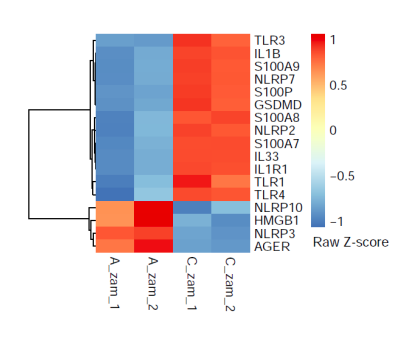
Heatmap of genes differentially expressed in the ZAM zone in relation to the sterile inflammation phenomenon.
Author Response
Reviewer #3 (Public Review):
The authors analyzed several models for predicting the early onset of T2D, where they trained and tested on a UKB based cohort, aged 40 - 69 and suggest two simple logistic regression models: the anthropometric and the five blood tests models in reference to FINDRISC and GDRS models. Their models achieved better auROC, APS, and decile prevalence OR, and better-calibrated predictions.
Strengths:
1.The authors have neatly explained their objectives and performed well-justified analyses.
2.The authors highlight how using both features - HbA1C% measure and reticulocyte count may provide a better indication of the average blood sugar level during the last two-three months than using just the standard HbA1C% measure.
3.Further verification of the proposed anthropometric-based and 5 blood-test results-based modelscan discriminate discriminating within a group of normoglycemic participants and within a group of pre-diabetic participants resulted in outperforming the FINDRISC and the GDRS based models.
Weaknesses:
- As the authors point out in the manuscript that these models are suited for the UKB cohort or populations with similar characteristics. It limits the extrapolation of these findings onto another cohort from a different background until analyzed on another country/continent-based cohort.
We agree with this comment as we indeed pointed in the paper. We recommend to adjust these models when applying it to populations with distinct characteristics.
- In the methods section, an additional explanation of how the T2D prevalence bins were formed would be useful to a reader.
We thank the reviewer for this note, we added the following explanation in section 4.11: “We considered several potential risk score limits that separate T2D onset probability in each of the scores groups, and we chose boundaries that showed a separation between the risk groups on the validation datasets. Once we decided on the boundaries of the score, we report the prevalence in each risk group on the test set and we report these results.”
- The authors have mentioned that the prevalence of diabetes has been rising more rapidly in low and middle-income countries (LMICs) than in high-income countries and the objective of the present research was to develop clinically usable models which are easy to use and highly predictive of T2D onset. As lifestyle is also one of the contributory factors for T2D, additional analysis that includes a comparison of groups between low-income and high-income subjects within UKB-based cohort provided such metadata available would help understand if the prevalence for T2D differs or not between such groups.
We thank the reviewer for this comment, we added below an analysis that we run on our data, showing the deprivation indexes differences between sick and healthy populations. The sick population has a higher deprivation index as expected. When running a Mann-Whitney U Test on the data we get a p value of zero, creating this with a sample of just 1000 participants from each group, we get a p-value of 2.37e-137. This indicates that there is a significant correlation between deprivation index and tendency to develop T2D. We also add this finding to the supplementary material and a reference to it.
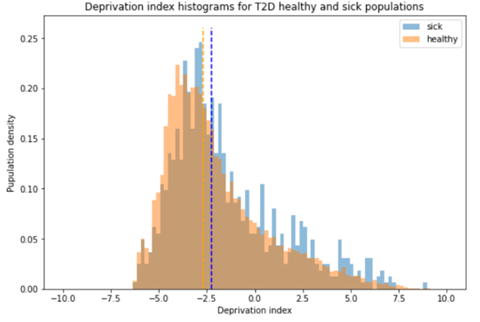
You can also find below a SHAP diagram showing tht higher Townsend deprivation index is pushing the prediction for T2D upwards.
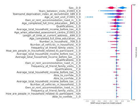
Author Response
Reviewer #2 (Public Review):
Summary: This substantial collaborative effort utilized virus-based retrograde tracing from cervical, thoracic and lumbar spinal cord injection sites, tissue clearing and cutting-edge imaging to develop a supraspinal connectome or map of neurons in the brain that project to the spinal cord. The need for such a connectome-atlas resource is nicely described, and the combination of the actual data with the means to probe that data is truly outstanding.
They then compared the connectome from intact mice to those of mice with mild, moderate and severe spinal cord injuries to reveal the neuronal populations that retain axons and synapses below the level of injury. Finally, they look for correlations between the remaining neuronal populations and functional recovery to reveal which are likely contributing to recovery and its variability after injury. Overall, they successfully achieve their primary goals with the following caveats: The injury model chosen is not the most widely employed in the field, and the anatomical assessment of the injuries is incomplete/not ideal.
Concerns/issues:
1) I would like to see additional discussion/rationale for the chosen injury model and how it compares to other more commonly employed animal models and clinical injuries. Please relate how what is being observed with the supraspinal connectome might be different for these other models and for clinical injuries.
We have added text to the Results and Discussion to explain our rationale for selecting the crush injury model, and to acknowledge differences between this model and more clinically relevant contusion models. (Results: line 360-364, Discussion 608-615). We agree wholeheartedly that a critical future direction will be to deploy brain-wide quantification in contusion models, and we are currently seeking funding to obtain the needed equipment.
2) The assessment of the thoracic injuries employed is not ideal because it provides no anatomical description of spared white matter (or numbers of spared axons) at the injury epicenter.
We address this more fully in the related point below. Briefly, we agree with a need to improve the assessment of the lesion but are hampered by tissue availability. We are unable to assess white matter sparing but can offer quantification of the width of residual astrocyte tissue bridges in four spinal sections from each animal (new Figure 5 – figure supplement 3). As discussed below, however, we recognize the limitations of the lesion assessment and agree with the larger point that the current quantification methods do not position us to make claims about the relative efficacy of spinal injury analyses versus whole-brain sparing analyses to stratify severity or predict outcomes. Our approach should be seen as a complement, not a substitute, for existing lesion-based analyses. We have edited language throughout the manuscript to make this position clearer.
3) Related to this, but an issue that requires separate attention is the highly variable appearance of the injury and tracer/virus injection sites, the variability in the spatial relationship with labeled neurons (lumbar) and how these differences could influence labeling, sprouting of axons of passage and interpretation of the data. In particular this is referring to the data shown in Figure 6 (and related data).
It is true that there is some variability in the relative position of the injury and injection, a surgical reality. The degree of variability was perhaps exaggerated in the original Figure 6 (Now Figure 5), in which one image came from one of two animals in the cohort with a notably larger gap between the injury and injection. Nevertheless, this comment raises the important question of how variability in injection-to-injury distance might affect supraspinal label. First, we would emphasize the data in Figure 1 – Figure Supplement 6, in which we showed that the number of retrogradely labeled supraspinal neurons is relatively stable as injection sites are deliberately varied across the lower thoracic and lumbar cord. Indeed, the question raised here is precisely the reason we performed this early test to determine how sensitive the results might be to shifts in segmental targeting. The results indicate that retrograde labeling is fairly insensitive to L1 versus L4 targeting. As an additional check for this specific experiment we also measured the distance between the rostral spread of viral label and the caudal edge of the lesion and plotted it against the total number of retrogradely labeled neurons in the brain. If a smaller injury/injection gap favored more labeling we might expect negative correlation, but none is apparent. We conclude that although the injury/injection distance did vary in the experiment, it likely did not exert a strong influence on retrograde labeling.
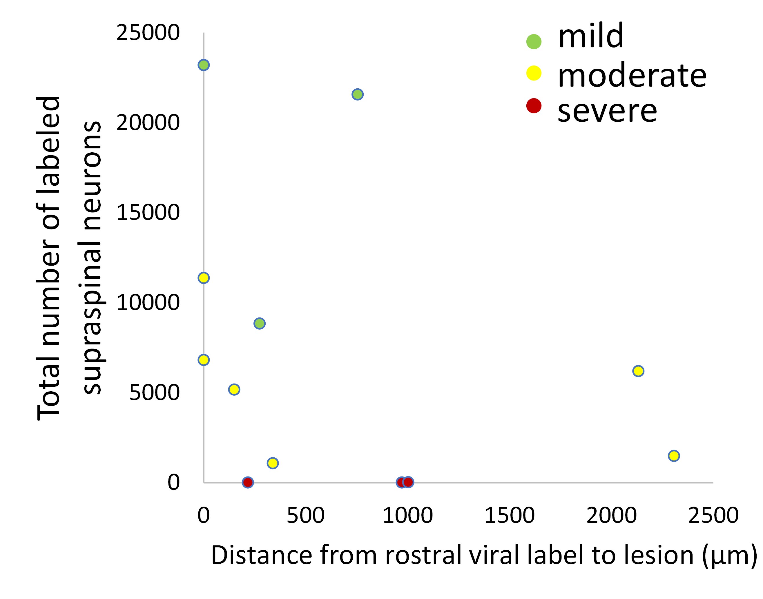
Reviewer #3 (Public Review):
In this manuscript, Wang et al describe a series of experiments aimed at optimizing the experimental and computational approach to the detection of projection-specific neurons across the entire mouse brain. This work builds on a large body of work that has developed nuclear-fused viral labelling, next-generation fluorophores, tissue clearing, image registration, and automated cell segmentation. They apply their techniques to understand projection-specific patterns of supraspinal neurons to the cervical and lumbar spinal cord, and to reveal brain and brainstem connections that are preferentially spared or lost after spinal cord injury.
Strengths:
Although this work does not put forward any fundamentally new methodologies, their careful optimization of the experimental and quantification process will be appreciated by other laboratories attempting to use these types of methods. Moreover, the observations of topological arrangement of various supraspinal centres are important and I believe will be interesting to others in the field.
The web app provided by the authors provides a nice interface for users to explore these data. I think this will be appreciated by people in the field interested in what happens to their brain or brainstem region of interest.
Weaknesses:
Overall the work is well done; however, some of the novelty claims should be better aligned with the experimental findings. Moreover, the statistical approaches put forward to understand the relationship between spinal cord injury severity and cell counts across the mouse brain needs to be more carefully considered.
The authors state that they provide an experimental platform for these types of analysis to be done. My apologies if I missed it but I could not find anywhere the information on viral construct availability or code availability to reproduce the results. Certainly both of these aspects would be required for people to replicate the pipeline. Moreover, the described methodology for imaging and processing is quite sparse. While I appreciate that this information is widely provided in papers that have developed these methods, I do not think it is appropriate to claim to have provided a platform for people to enable these types of analyses without a more in-depth description of the methods. Alternatively, the authors could instead focus on how they optimized current methodologies and avoid the overstatement that this work provides a tool for users. The exception to this is of course the viral constructs, the plasmids of which should be deposited.
We agree that we have not provided a tool per se, more of an example that could be followed. We have revised language in the abstract, introduction, and discussion to make it clear that we optimized existing methods and provide an example of how this can be done, but are not offering a “plug and play” solution to the problem of registration that would, for example, allow upload of external data. For example, in the abstract we replaced “We now provide an experimental platform” with “Here we assemble an experimental workflow.” (Line 28). The term “platform” no longer appears in the manuscript and has been replaced throughout by “example.” We how this matches the intention of the comment and are happy to revise further as needed. Note that the plasmids have been deposited to Addgene.
It was not completely to me clear why or when the authors switch back and forth between different resolutions throughout the manuscript. In the abstract it states that 60 regions were examined, but elsewhere the number is as many as 500. My understanding is that current versions of the Allen Brain Annotation include more than 2000 regions. I think it would make things clear for the readers if a single resolution was used throughout, or at least justified narratively throughout the text to avoid confusion.
Thank you for pointing this out. The Cellfinder application recognizes 645 discrete regions in the brain, and across all experiments we detected supraspinal nuclei in 69 of these. This number, however, includes some very fine distinctions, for example three separate subregions of vestibular nuclei, three subregions of the superior olivary complex, etc. True experts may desire this level of information, but with the goal of accessibility we find it useful to collapse closely related / adjacent regions to an umbrella term. Doing so generates a list of 25 grouped or summary regions. In the revised version we move the 69-region data completely to the supplemental data (there for the experts who wish to parse), and use the consistent 25-region system (plus cervical spinal cord in later sections) to present data in the main figures. We have added text to the Results section (lines 157-162) to clarify this grouping system.
The others provide an interesting analysis of the difference between cervical and lumbar projections. I think this might be one of the more interesting aspects of the paper - yet I found myself a bit confused by the analysis, and whether any of the differences observed were robust. Just prior to this experiment the authors provide a comparison of the mScarlet vs. the mGL, and demonstrate that mGL may label more cells. Yet, in the cervical vs. lumbar analysis it appears they are being treated 1 to 1. Moreover, I could not find any actual statistical analysis of this data? My impression would be that given the potential difference in labelling efficiency between the mScarlet and mGL this should be done using some kind of count analysis that takes into account the overall number of neurons labelled, such as a Chi-sq test or perhaps something more sophisticated. Then, with this kind of statistical analysis in place, do any of the discussed differences hold up? If not, I do not think this would detract from the interesting topological observations - but would call on the authors to be a bit more conservative about their statements and discussion regarding differences in the proportions of neurons projecting to certain supraspinal centers.
This is an important point. In response to this input and related comments from other reviewers we performed new experiments to assess co-localization. The new data address the point above by including quantification of the degree of colocalization that results from titer-matched co-injection of the two fluorophores, providing baseline data. The results of this can be found in Figure 3 – figure supplement 3 and form the basis for statistical comparisons to experimental animals shown in Figure 3.
Finally, I do have some concerns about the author's use of linear regression in their analysis of brain regions after varying severities of SCI. First of all, the BMS score is notoriously non-linear. Despite wide use of linear regressions in the field to attempt to associate various outcomes to these kinds of ordinal measures, this is not appropriate. Some have suggested a rank conversion of the BMS prior to linear analyses, but even this comes with its own problems. Ultimately, the authors have here 2-3 clear cohorts of behavioral scores and drawing a linear regression between these is unlikely to be robustly informative. Moreover, it is unclear whether the authors properly adjusted their p-values from running these regressions on 60 (600?) regions. Finally, the statement in the abstract and discussion that the authors "explain more variability" compared to typical lesion severity analysis is also unsupported. My suggestion would be the following:
Remove the linear regression analyses associated with BMS. I do not think these add value to the paper, and if anything provide a large window of false interpretation due to a violation of the assumptions of this test.
Consider adding a more appropriate statistical analysis of the brain regions, such as a non-parametric group analysis. Knowing which brain regions are severity dependent, and which ones are not, would already be an interesting finding. This finding would not be confounded by any attempt to link it to crude measures of behavior.
We agree that the linear regression approach was flawed and appreciate the opportunity to correct it. After consultation with two groups of statisticians we were forced to conclude that the data are simply underpowered for mixed model and ranking approaches. We therefore adopted a much simpler strategy. As you point out (and as noted by the statisticians), the behavioral data are bimodal; one group of animals regained plantar stepping ability, albeit with varying degrees of coordination (BMS 6-8), while the others showed at most rare plantar steps (BMS 0-3.5). We therefore asked whether the number of spared neurons in each brain region differed between the two groups and also examined the degree of “overlap” in the sparing values between the two groups. The data are now presented in Figure 6.
If the authors would like to state anything about 'explaining more variability' then the proper statistical analysis should be used, which in this case would be to compare the models using a LRT or equivalent. However, as I mentioned it does not seem to be appropriate to be doing this with linear models so the authors should consider a non-linear equivalent if they choose to proceed with this.
We thank the reviewer for the excellent suggestion. However as we explained above after consultation with two groups of statisticians we were forced to conclude that the data are underpowered and could not apply some of the methods suggested. Especially in light of our simplified analysis, we think it is better to remove any claims of the relative success of the sparing in different regions to explain more or less variability. Instead we can simply report that sparing in some regions, but not others, is significantly different between “low-performing” and “high-performing” groups.
Author Response:
Reviewer #1 (Public Review):
This paper focuses on the role of historical evolutionary patterns that lead to genetic adaptation in cytokine production and immune mediated diseases including infectious, inflammatory, and autoimmune diseases. The overall goal of this research was to track the evolutionary trajectories of cytokine production capacity over time in a number of patients with different exposure to infectious organisms, infectious disease, autoimmune and inflammatory diseases using the 500 Functional Genomics cohort of the Human Functional Genomics Project. The identified cohort is made up of 534 individuals of Western European ancestry. Much of this focus is on the impact and limitations of certain datasets that they have chosen to use such as the "average genotyped dosage" to be substituted for missing variants and data interpretation.
We fully agree with the reviewer, we replace missing variants in a sample with its average dosage in the entire dataset. This makes it so missing variants in a sample do not bias the trends over time we observe. If we were to correct it using only samples from within their own era we would be inflating differences between the different era's. Whereas only using shared variants would increase the noise for older samples due to higher error rates associated with DNA degradation.
Moreover, some data pairings in the data set are not complete or had varying time points .
The stimulation periods were chosen based on extensive studies that showed that the timepoints used were best suited for assessing monocyte-derived and lymphocyte-derived cytokines per stimulus. Not all the stimuli induce the production of all cytokines, so the selection of the cytokine-stimulus pairs was performed for those pairs in which a cytokine production could be measured (PMID: 1385767; PMID: 19380112; PMID: 27814509; PMID: 27814508; PMID: 27814507). The differences in the cytokine availability and time points are adjusted to the optimal time of production per stimuli. Monocyte-derived cytokines (IL-1b, IL-6 and TNFa) are early response cytokines, produced by innate immune cells shortly after stimulation. IFNg, IL-17 and IL-22 are lymphocyte-derived cytokines, produced by adaptive immune cells, in this case T helper cells. These cells need to differentiate for several days before they start to produce these cytokines, this is the reason why the time point of the measurements of these cytokines is 7 days. In the case of IFNg, it can also be produced by NK cells, so it was measured after 48h after stimulation in whole blood samples. We have included these considerations in the new version of the text (lines 82 to 87).
Similarly, a split was done to look at before and after the Neolithic era and the linear regression correspond to those two eras. However, the authors do not comment or show the data to demonstrate why they choose that specific breakpoint as opposed to looking at every historical era transition, i.e., from early upper paleolithic to late upper paleolithic to Mesolithic to Neolithic to post-Neolithic to modern.
We thank the reviewer for this remark and acknowledge that we do not address the rationale behind our choice to look at this split specifically sufficiently. We hypothesized that the start of the Neolithic with its increase in population density and contact with animals would also be a turning point for many immune responses and immune related traits. We added various analyses to better highlight this and also show differences between different adjacent time periods.
-The original figures showed only models using two separate linear regression lines and the different thresholds for missing genotype rates showed consistent results. In the new figures we depict LOESS regression models to better show the difference in mean PRS at every point in time and we additionally show boxplots with the different major age periods pooling the paleolithic and mesolithic samples together as pre-neolithic samples in order to account for the lower sample number in the earlier historical periods. To highlight this we have added a new section in lines 123 to 129 and new versions of the figures 1, 2, 3 and 4.
-In the new figure 2 we add LOESS regression models for which we do not bias our analysis into defining a break at a certain time period. We furthermore show boxplots with pairwise comparisons (student’s T-test) for broader time periods highlighting the changes in PRS that would correspond with major changes in human lifestyle such as the shift from a hunter-gatherer to a neolithic lifestyle or the rapid urbanization of human society.
-In the new Figure 3 we confirm that the various traits showing a clear change in PRS start at the advent of the Neolithic or post-Neolithic era using both the LOESS regression and pairwise comparisons (student T-test).
-Similarly the heatmap in our original figure 4 has also been revised to only show the large sample set.
Lastly, the authors should highlight additional limitations of this current study in terms of the generalizability to other populations or to clearly state that this is limited to the European population at the specified latitude and longitudes used.
We thank the reviewer for his feedback and agree we should put more emphasis on this. In our study we focus on summary statistics obtained from European populations and only employ European aDNA samples, so our results should not be extrapolated to other populations from other geographical areas. We have included this in the Discussion of the new version of the manuscript (lines 289 to 292). However, our findings are mostly in agreement with previous studies in other populations, which adds robustness to the results of our study.
Reviewer #2 (Public Review):
In "Evolution of cytokine production capacity in ancient and modern European populations", Dominguez-Andrés et al. collect a large amount of trait association data from various studies on immune-mediated disorders and cytokine production, and use this data to create polygenic scores in ancient genomes. They then use the scores to attempt to test whether the Neolithic transition was characterized by strong changes in the adaptive response to pathogens. The impact of pathogens in human prehistory and the evolutionary response to them is an intriguing line of inquiry that is now beginning to be approachable with the rapidly increasing availability of ancient genomes.
While the study shows a commendable collection of association data, great expertise in immune biology and an interesting study question, the manuscript suffers from severe statistical issues, which makes me doubt the validity and robustness of their conclusions. I list my concerns below, in rough order of how important I believe they are to the claims of the paper:
—In addition to the magnitude of an effect away from the null, P-values are a function of the amount of data one has to fit a model or test a hypothesis. In this case, the authors have vastly more data after the Neolithic Revolution than before, and so have much higher power to reject the null hypothesis of "no relationship to time" after the revolution than before. One can see this in the plots the authors provided, which show vastly more data after the Neolithic, and consequently a greater ability to fit a significant linear model (in any direction) afterwards as well.
We thank the reviewer for raising this very important point. In order to account for this difference in sample size for the different historical periods we pooled all samples prior to the neolithic era together to test for differences in mean PRS between neighbouring historical periods. This way we lose some strength in terms of the carbon-dated age of each sample but we gain the ability to compare more different pairings than just pre- and post-neolithic samples. We added various analyses to better highlight this and also show differences between different adjacent time periods:
-The original figures showed only models using two separate linear regression lines and the different thresholds for missing genotype rates showed consistent results. In the new figures we depict LOESS regression models to better show the difference in mean PRS at every point in time and we additionally show boxplots with the different major age periods pooling the paleolithic and mesolithic samples together as pre-neolithic samples in order to account for the lower sample number in the earlier historical periods. To highlight this we have added a new section in lines 123 to 129 and new versions of the Figures 1, 2, 3 and 4.
-In the new figure 2 we add LOESS regression models for which we do not bias our analysis into defining a break at a certain time period. We furthermore show boxplots with pairwise comparisons (student’s T-test) for broader time periods highlighting the changes in PRS that would correspond with major changes in human lifestyle such as the shift from a hunter-gatherer to a neolithic lifestyle or the rapid urbanization of human society.
-In the new figure 3 we confirm that the various traits showing a clear change in PRS start at the advent of the Neolithic or post-Neolithic era using both the LOESS regression and pairwise comparisons (student T-test).
-Similarly the heatmap in our original figure 4 has also been revised to only show the large sample set.
—The authors argue that Figure S2 makes their results robust to sample size differences, but showing a consistency in direction before and after downsampling in the post-neolithic samples is not enough, because:
1) you still lack power to detect changes in direction before the Neolithic.
2) even for the post-Neolithic, the relationship may be in the same direction but no longer significant after downsampling. How much the significance of the linear model fit is affected by the downsampling is not shown.
We thank the reviewer for pointing this out. The low sample count dating back to before the Neolithic era makes it indeed hard to accurately detect changes in PRS significantly correlated with time. Instead, we now aim to pool these samples together and compare the distribution of their PRS with those of Neolithic samples to better be able to detect significant differences in PRS between these historical time periods.
In order to show the significance of each linear model as well we now show the -Log10 of the P value multiplied by the sign of the correlation coefficient. This way we can better highlight the consistency in direction as well as significance and show that downsampling affects the order of significance. Please see the new Figure 4-figure supplement 1. We have also discussed this more in depth on lines 267-272 of the new version of the text.
—The authors chose to test "relationship between PRS with time" before and after the Neolithic as a way to demonstrate that "the advent of the Neolithic was a turning point for immune-mediated traits in Europeans". A more appropriate way to test this would be creating a model that incorporates both sets of scores together, accounts for both sample size and genetic drift in the change of polygenic scores, and shows a significant shift occurs particularly in the Neolithic, rather in any other time period, instead of choosing the Neolithic as an "a priori" partition of the data. My guess is that one could have partitioned the data into pre- and post-Mesolithic and gotten similar results, largely due to imbalances in data availability.
We agree with the reviewer that the exact pairing of the groups might influence the conclusions, showing the importance of remaining unbiased in our a priori partitioning of the data like the reviewer accurately pointed out. We aim to account for sample imbalances by pooling the paleolithic and mesolithic samples together and instead of just testing pre- versus post- Neolithic samples we perform a pairwise comparison between neighbouring historical periods using a T test thereby taking into account the sample size of each group.
—The authors only talk about partitions before and after the Neolithic, but plots are colored by multiple other periods. Why is the pre- and post-Neolithic the only transition that is mentioned?
Our initial hypothesis was that the pre-versus post-Neolithic shift was a turning point for immune responses. However, based on the suggestions of the reviewers, we have decided to perform the analysis in a more unbiased way, so we show the comparison of different individual era's. The new analyses and the new Figures provided address these issues.
—Extrapolating polygenic scores to the distant past is especially problematic given recent findings about the poor portability of scores across populations (Martin et al. 2017, 2019) and the sensitivity of tests of polygenic adaptation to the choice of GWAS reference used to derive effect size estimates (Berg et al. 2019, Sohail et al. 2019). In addition to being more heavily under-represented, paleolithic hunter-gatherers are the most differentiated populations in the time series relative to the GWAS reference data, and so presumably they are also the genomes for which PGS estimates built using such a reference would have higher error (see, e.g. Rosenberg et al. 2019). Some analyses showing how believable these scores are is warranted (perhaps by comparing to phenotypes in distant present-day populations with equivalent amounts of differentiation to the GWAS panel).
A similar study regarding standing height in ancient populations (PMID: 31594846) validated this approach when comparing polygenic scores based on modern populations with skeletal remains from ancient individuals. We do acknowledge the absolute results of the polygenic scores are less accurate for aDNA samples compared to a modern European cohort. The effect size estimates gained using a modern cohort are less accurate for aDNA samples than unrelated modern samples, and this is certainly an unavoidable limitation of the study.This is the reason why we focus on the direction of change of the trends and not on the absolute polygenic scores since such subtle differences do not affect the conclusions of our study.
—In multiple parts of the paper, the authors mention "adaptation" as equivalent to the patterns they claim to have found, but alternative hypotheses like genetic drift are not tested (see e.g. Guo et al. 2018 for a review of methods that could be used for this).
We thank the reviewer for this feedback. Based on this, we have added an Fst based test for selection to determine whether the changes we see in PRS over time are due to selection or due to genetic drift. This test shows that changes between the pre-Neolithic to Neolithic are not significantly different from drift whereas after the onset of the Neolithic we do see significant amount of selection. We have explained this further in the manuscript on lines 130-135 and included the new Table S2.

New Table S2 : Tests for selection as opposed to genetic drift were performed between populations from adjacent time periods. A two tailed test was used to determine whether mean trait Fst between pre-Neolithic - Neolithic, Neolithic - post-Neolithic, and post-Neolithic - Modern samples was significantly different compared to 10000 random LD and MAF matched mean Fst’s calculated using a same amount of SNP’s.
—250 kb window is too short a physical distance for ensuring associated loci that are included in the score are not in LD, and much shorter than standard approaches for building polygenic scores in a population genomic context (e.g. see Berg et al. 2019, Berisa et al. 2016). Is this a robust correction for LD?
We thank the reviewer for this remark, we tested multiple thresholds for window sizes, increasing the window size from 250 kb to 500 kb and 1000 kb (please see below new Figure 1-figure supplement 2) Although the level of significance changes for a few traits, the direction of the change remains stable across the three thresholds, demonstrating the robustness of our results. We have chosen this approach because the aDNA samples present a too high error rate and contain a relatively high amount of missing data to accurately determine LD, and determining LD using a modern reference cohort would bias our analysis by assuming the aDNA samples have a similar LD structure as modern samples.
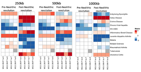
New Figure 1-figure supplement 2: PRS correlation pre- and post-Neolithic revolution using polygenic scores calculated at varying window sizes.
We have edited the manuscript accordingly to show the consistency between these varying window sizes on lines 111-113.
—If one substitutes dosage with the average genotyped dosage for a variant from the entire dataset, then one is biasing towards the partitions of the dataset that are over-represented, in this case, post-Neolithic samples.
We fully agree with the reviewer, however the substitution of missing dosages with average dosages prevents the introduction of the bias in our models caused by varying amounts of missing SNPs in the older samples. Although our average scores on an absolute level are largely influenced by the more abundant post-Neolithic samples, this reduces the odds of wrongfully observing significant trends caused by the sparsity of the data. While the absolute scores might be biased towards a certain value, the differences and thus the direction of the change in PRS is affected by the non-missing variants in each sample.
—It seems from Figure 2, that some scores are indeed very sensitive to the choice of P-value cutoff (e.g., Malaria, Tuberculosis) and to the amount of missing data (e.g. HIV). This should be highlighted in the main text.
The reviewer is right, and this is largely due to the fewer number of SNPs that are included in the model at stricter p-value cutoffs, which is in part a limitation of the available GWAS summary statistics. Using fewer SNPs in our PRS calculations reduces the variability between different samples which weakens our ability to accurately model changes in these specific complex traits and detect statistical significance. We have highlighted this in the main text on lines 193-196.
—Some of the score distributions look a bit strange, like the Tuberculosis ones in Figure 2, which appear concentrated into particular values. Could this be because some of the scores are made with very few component SNPs?
We thank the reviewer for pointing this out and this is indeed correct. At stricter thresholds fewer significant QTLs will be included in the polygenic score model. We chose to still show these plots to point out those results might more easily differ if more variants could be included. At more lenient thresholds more variants can be included increasing the power of the model but the score might be less informative for the trait that way.
Author Response
Reviewer #3 (Public Review):
Myelodysplastic syndrome (MDS) is a heterogenous, clonal hematopoietic stem cell disorder characterized by morphological dysplasia in one or more hematopoietic lineages, cytopenias (most frequently anemia), and ineffective hematopoiesis. In patients with MDS, transfusion therapy treatment causes clinical iron overload; however it has been unclear if treatment with iron chelation yields clinical benefits. In the present study, the authors use a transgenic mouse model of MDS, NUP98-HOXD13 (referred to here as "MDS mice") to investigate this area. Starting at 5 months of age (before MDS mice progress to acute leukemia), the authors administered DFP in the drinking water for 4 weeks, and compared parameters to untreated MDS mice and WT controls.
The authors first show that MDS mice exhibit systemic iron overload and macrocytic anemia that is improved by treatment with the iron chelator deferiprone (DFP). They then perform a detailed characterization the effects of DFP treatment on erythroid differentiation and various parameters related to iron transport and trafficking in MDS erythroblasts. Strengths of the work are the use of a well-characterized mouse model of MDS with appropriate animal group sizes and detailed analyses of systemic iron parameters and erythroid subpopulations. A remediable weakness is that in certain areas of the Results and Discussion, the authors overinterpret their findings by inferring causation when they have only shown a correlation. Additionally, when drawing conclusions based on changes in erythroblast mRNA expression levels between groups, the authors should consider that translation efficiency may be altered in MDS and that the NUP98 fusion protein itself, by acting as a chimeric transcription factor, may also impact gene expression profiles. Given that the application of chelators for treatment of MDS remains controversial, this work will be of interest to scientists focused on erythroid maturation and iron dysregulation in MDS, as well as clinicians caring for patients with this disorder.
Major Comments
1) The authors define the stages of erythroblast differentiation using the CD44-FSC method, which assumes that CD44 expression levels during the stages of erythroid differentiation are not altered by MDS itself. Are morphologically abnormal erythroblasts, such as bi-nucleate forms, captured in this analysis, and if so, are they classified in the appropriate subset? The percentage of erythroblasts in the bone marrow of MDS mice in this current study is lower than that reported by Suragani et al (Nat Med 2014), who employed a different strategy to define erythroid precursors. While representative erythroblast gating is presented as Supplemental Figure 17, it would be important to present representative gating from all 3 animal groups: WT, MDS, and MDS+DFP mice.
We appreciate this comment and have added representative gating for all 3 groups to Supplemental Figure 17 (new Figure 3 – figure supplement 6 in the revised manuscript).
2) Methods, "Statistical analysis." The authors state that all comparisons were done with 2-tailed student paired t test, which would not be appropriate for comparisons being made between independent animals groups (i.e. when groups are not "paired").
We appreciate this comment and have reanalyzed all revised mouse data using one-way ANOVA with multiple comparisons and Tukey post-test analyses when more than 2 groups were compared. This has been edited in the Methods section in the revised manuscript.
3) The Results (p.7) indicates that both sexes showed similar responses to DFP; however, the figure legends do not indicate sex. Given that systemic iron metabolism in mice shows sex-related differences, sex should be specified.
We appreciate this comment and present here the gender-specific data for the reviewers’ evaluation (Author respone image 1). Similarly elevated transferrin saturation (a) (n = 3-4 male mice/group and n = 4-6 female mice/group) and hemoglobin (b) (n = 4-6 male mice/group and n = 4-9 female mice/group) are observed in male and female DFP-treated MDS mice. (c) Bone marrow erythroblasts are decreased to a greater degree in male relative to female DFP-treated MDS mice (n = 4-7 male mice/group and n = 8-9 female mice/group). We have added the data on gender-specific measures to new Figure 1 - figure supplement 3, Figure 2 – figure supplement 1, and Figure 3 – figure supplement 1 in the revised manuscript.
Author respone image 1.
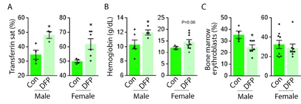
Author Response
Reviewer #1 (Public Review):
The manuscript by Xu et. al. does a very thorough characterization and molecular dissection of the role of SSH2 in spermatogenesis. Loss of SSh2 in germ cells results in germ cell arrest In step2-3 spermatids and eventually leads to germ cell loss by apoptosis. Molecular characterization of the mutant mice shows that the loss of SSH2 prevents the fusion of proacrosomal vesicles leading to the formation of a fragmented acrosome. The fragmentation of the acrosome is due to the impaired actin bundling and dephosphorylation of COFILIN. In short, this is a comprehensive body of work.
We thank the referee for these insightful comments.
Reviewer #2 (Public Review):
The acrosome is a unique sperm-specific subcellular organelle required for the fertilization process, and it is also an organelle undergoing extensive morphological and structural transformation during sperm development. The mechanism underlying the extensive acrosome morphogenesis and biogenesis remains incompletely understood. Xu et al in their manuscript entitled "The Slingshot phosphatase 2 is required for acrosome biogenesis during spermatogenesis in mice" reported that the Slingshot Phosphatase 2 is essential for acrosome biogenesis and male fertility through their characterization of spermatogenic and acrosomal defects in Ssh2 knockout mice they generated. Specifically, the authors provided molecular, genetic, and subcellular evidence supporting that Ssh2 mutation impaired the phosphorylation of an acting-binding protein, COFILIN during spermiogenesis and accordingly actin cytoskeleton remodeling, crucial for proacrosomal vesicle trafficking and acrosome biogenesis. The manuscript by Xu et. al. does a very thorough characterization and molecular dissection of the role of SSH2 in spermatogenesis. Loss of SSh2 in germ cells results in germ cell arrest In step2-3 spermatids and eventually leads to germ cell loss by apoptosis. Molecular characterization of the mutant mice shows that the loss of SSH2 prevents the fusion of proacrosomal vesicles leading to the formation of a fragmented acrosome. The fragmentation of the acrosome is due to the impaired actin bundling and dephosphorylation of COFILIN. In short, this is a comprehensive body of work.
We appreciate and thank Referee #2 for the positive feedback and insightful comments.
Strengths:
Nicely written manuscript, addresses an important mechanistic question of the roles of cytoskeleton remodeling in acrosome biogenesis and provided genetic, subcellular, and molecular evidence to build up their support for their hypothesis that Ssh2 regulates actin cytoskeleton remodeling, a process essential for proacrosomal vesicle trafficking and acrosome biogenesis, through dephosphorylation actin-binding protein during spermiogenesis.
We again thank to the Referee #2 for appreciating and encouraging us regarding our current research work.
Weaknesses:
For body weight, and testis weight of the mutants, the authors concluded that there is no significant difference between the mutant and wildtype (Fig 1E -1G), but they appear to use mice between 6-8 wk old, both the testis and body weight of males at 6-8 wks is still growing, with the number of mice analyzed being six, you could easily miss the significant difference of the testis size and or body weight with such a varied age and a small sample size.
We thank the referee for their prompting of this important discussion point, which we now cover in our revised manuscript. In our originally submitted manuscript, we only presented the data for body weight, testis weight, and T/B ratio for mice between the age of 6–8 weeks, however, we have added the additional data of mice with age more than 8 weeks in the revised manuscript in a new Figure 1E-1G with the sample size of 12 for each genotype. We have also updated the relevant content in the figure caption. The revised figure caption for Figure 1 panels E–G reads as follows: “(E-G) Body weights (26.3609 ± 0.4914 for WT; 25.1741 ± 0.5189 for Ssh2 KO), weights of the testes (0.0862 ± 0.0036 for WT; 0.0788 ± 0.0023 for Ssh2 KO), and the testis-to-body weight ratio (0.3281 ± 0.0153 for WT; 0.3154 ± 0.0135 for Ssh2 KO) of adult WT and Ssh2 KO males (n = 12). Data are presented as the mean ± SEM; p > 0.05 calculated by Student’s t-test. Bars indicate the range of the data.”
Other points:
Comments: 1) Could the uniform cytoplasmic distribution of diminutive actin filaments in the wild type and disrupted actin filament remodeling be examined at the EM level on the round spermatids?
We apologize for the confusion. Previously, we conducted a transmission electron microscopy (TEM) analysis on the testes samples to discover the distribution and ultrastructural organization of F-actin in WT and Ssh2 KO round spermatids. Unfortunately, even at high magnification (30,000x, right panel of Figure R1-Response Figure 1) by TEM of testicular section no diminutive actin filament was observed in the cytoplasm of round spermatids except for the acroplaxome-an actin-rich specialized structure anchors the acrosome-in WT spermatids as well as some thick bundle-like structures located at the acrosomal region of Ssh2 KO spermatids (Fig. R1). According to their unique characteristic of appearance, we interpreted these electron-dense bundles as the aberrantly aggregated actin filaments whose lengths are in accordance with the lengths of COFILIN-saturated F-actin fragments (Bamburg et al., 2021), suggesting the disrupted actin filament remodeling during acrosome biogenesis resulted from Ssh2 KO. However, due to the technological limitations of TEM and the complexity of intracellular environment of round spermatids, we only recognized few aggregated actin bundles with the loss of filamentous appearance in Ssh2 KO spermatids and no typical diminutive actin filament was detected which had been imaged under high-resolution cryo-TEM (Haviv et al., 2008) or live-cell total internal reflection fluorescence microscopy (Johnson et al., 2015) on the purified actin bundles and cultured cells. Given the lack of effective approaches to culture murine round spermatids in vitro, confocal microscopy of flourescence-labelled F-actin (e.g., IF staining by FITC-phalloidin) is a more accessible method for visualizing the disruption of actin remodeling than EM in murine spermatids as the actin-related findings that several other studies demonstrated (Djuzenova et al., 2015; Meenderink et al., 2019).
Comments: 2) Any other defects are seen besides acrosome in the mutant testis given the important roles of actin cytoskeleton network and high expression of Ssh2 in spermatocytes, were chromatoid bodies or mitochondria affected in any way? Any other defects in the mice overall including female fertility and other organs, given the previously reported roles in the nervous system. It could be helpful information for others interested in Ssh 2 protein and actin cytoskeleton's roles in general.
The referee has here raised an interesting point. Firstly, besides the acrosome-related defects in Ssh2 KO spermatids, we identified increased germ cell apoptosis and aberrant activation of apoptotic Bcl-2/Caspase-3 pathway in the testes of Ssh2 KO mice which were speculated to be triggered by the disordered COFILIN-mediated F-actin remodeling and have attracted our attention to further elucidate the underlying mechanisms in the future. Secondly, given the high expression of SSH2 in spermatocytes demonstrated by IF staining shown in figure 4B and 4C,we thus performed the surface chromosome spreading on spermatocytes to observe whether the morphology of chromatid bodies and the meiotic progression was affected by Ssh2 KO and no obvious defects were observed as shown in supplementary Figure S3 in originally submitted manuscript. Thirdly, no obvious morphological abnormality in chromatin or mitochondrial structure was detected in Ssh2 KO germ cells such as spermatocytes and round spermatids under TEM which prevents us to pursue it further. Fourthly, we have observed the potential effect(s) of Ssh2 KO on female fertility using Ssh2 KO female mice and did not find any obvious infertility defect in Ssh2 KO females compared to their WT littermates as demonstrated by the data of the body weight, ovary weight, ovary-to-body weight ratio, size of ovaries and fertility test as well as the images of ovarian HE staining (Fig. R1). Moreover, given that during our investigation period, Ssh2 KO males and females did not manifest any defective physical development, aberrant physiological status or mental disorder notwithstanding the roles of SSH2 in neurite extension had been reported (Endo, Ohashi, & Mizuno, 2007), we did not conduct the experiments to observe the effect(s) of SSH2 in other organs except for the female fertility.
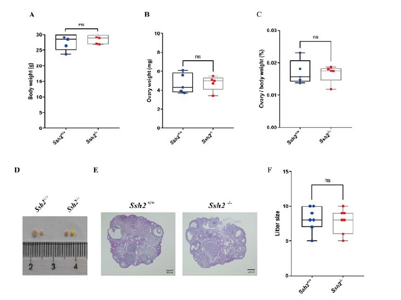
Fig. R1 No reproductive defects were found in Ssh2 KO females. (A-C) Body weights, weights of the ovaries, and the ovary-to-body weight ratio of adult WT and Ssh2 KO females aged 8-10 weeks (n = 5); p > 0.05 calculated by Student’s t-test. Bars indicate the range of data. (D) The size of ovaries from Ssh2 KO were indistinguishable from ovaries of WT mice age 8 weeks, n = 4. (E) Histology of the ovaries from WT and Ssh2 KO mice. Sections were stained with hematoxylin and eosin. Scale bars: 200 μm. Images are representative of ovaries extracted from 8-week-old adult female mice per genotype. (F) Number of pups per litter from WT and Ssh2 KO male mice (8 weeks old) after crossing with WT adult male mice (n =3); p > 0.05 calculated by Student’s t-test. Bars indicate the range of the data.
Comments: 3) Providing detailed information on the number of animals used and cells analyzed in the legend is nice, but it might be even better for the readers to include sample size and the number of cells examined in the figure/graph if possible.
We appreciate the suggestions from the reviewer. We have integrated some information of sample size in the figures where appropriate. Firstly, we integrated sample size in the figure 1C, 1E, 1F, 1G and 1I. Secondly, we included sample size and the number of seminiferous tubule/epididymal duct we evaluated for TUNEL (+) cell counting in figure 2C and figure 2D. Thirdly, we included sample size and the number of spermatids for co-localization in figure 6B and figure 6D.
Comments: 4) Nice discussion and comparison with GOPC and GM130, how about comparison and discussion with other acrosome defective mutants like PICK1, and ATG to provide some insights into acrosome biogenesis and proacrosomal vesicle trafficking?
We greatly appreciate the referee for positive appraisal of our work with constructive suggestions, unfortunately, we are unable to address these defective mutants with certainty due to the lack of proper sample accessibility (only 3 of 16-month-old Ssh2 KO mice are accessible now). We compared the cytological staining of GM130 and GOPC in WT and Ssh2 KO spermatids using tubule squash sections as the description in the originally submitted manuscript which are prepared from fresh testes originated from 8-week-old mice and we now have several aged Ssh2 KO mice which prevent us to achieve the staining of PICK1 and ATG. PICK1 was previously reported to facilitate vesicle trafficking from the Golgi apparatus to the acrosome which co-localizes with GOPC in the proacrosomal granules (Xiao et al., 2009) and the phenotypes of Pick1 KO mice share a lot of similar characteristics with that of Ssh2 KO mice such as the fragmentation of the acrosome and increased germ cell apoptosis. Both autophagy-related ATG5 (Huang et al., 2021) and ATG7 (Wang et al., 2014) were reported to participate in the process of acrosome biogenesis and ATG7 is required for proacrosomal vesicle transportation/fusion by conjugating LC3 to the membrane of proacrosomal vesicles. Although the spermatids evaluated in these KO mice models could still be developed into spermatozoa with defective acrosome that is different from the situation in Ssh2 KO mice, it would be meaningful to discover the affects by Ssh2 KO on the localization of these regulators of acrosome biogenesis in spermatids and their potential interactions with SSH2. Indeed, in future work, we plan to pursue these issues and the content related to PICK1 has been added to the discussion in the revised manuscript as follows: “Moreover, it is intriguing to note that the phenotypes of Ssh2 KO mice share a lot of similarities with that of Pick1 KO model (Xiao et al., 2009) such as acrosome fragmentation and enhanced germ cell apoptosis, suggesting the possibility that SSH2 and PICK1 work together in a same trafficking machinery functioning in acrosome biogenesis which needs to be clarified further.”
Comments: 5) Given the literature on Cofilin's requirement for male fertility and the increased p-Cofilin in Ssh2 mutant testis by Western and IF, the authors have a strong case for their hypothesis. But given the general role of phosphatase, it might be prudent to discuss alternative possibilities.
We thank the reviewer for these valuable suggestions. Given that p-COFILIN is the only known substrate of SSH2 based on previous reports, we focused principally on this cascade to conduct our investigation. As a phosphatase, SSH2 is very likely to interact with many other proteins functioning in various cellular processes other than the actin-binding proteins which remain elusive. As directed, we now have added some content related to the regarding above concern in the discussion section of the revised manuscript as follows: “Given the diverse physiological roles reported for Slingshot family proteins, the possibility of the alternative mechanism underlying involvement of SSH2 in cellular events beyond the COFILIN-mediated actin remodeling should be noted. According to some publicly accessible databases as the indicators of potential protein–protein interactions such as BioGRID (Oughtred et al., 2019) and IntAct (Del Toro et al., 2022), SSH2 might interact with a set of actin-based molecular motors covering MYH9, MYO19 and MYO18A, which have been implicated in the maintenance of Golgi morphology and Golgi anterograde vesicular trafficking via the PI4P/GOLPH3/MYO18A/F-actin pathway (Rahajeng et al., 2019).”
Author Response
Reviewer #2 (Public Review):
Zylbertal and Bianco propose a new model of trial-to-trial neuronal variability that incorporates the spatial distance between neurons. The 7-parameter model is attractive because of its simplicity: A neuron's activity is a function of stimulus drive, neighboring neurons, and global inhibition. A neuroscientist studying almost any brain area in any model organism could make use of this model, provided that they have access to 1) simultaneously-recorded neurons and 2) the spatial locations of those neurons. I could foresee this model being the de-facto model to compare to all future models, as it is easy to code up and interpret. The paper explores the effectiveness of this distance model by modeling neural activity in the zebrafish optic tectum. They find that this distance-based model can capture 1) bursting found in spontaneous activity, 2) ongoing co-fluctuations during stimulus-evoked activity, and 3) adaptation effects during prey-catching behavior.
Strengths:
The main strength of the paper is the interpretability of the distance-based model. This model is agnostic to the brain area from which the population of neurons is recorded, making the model broadly applicable to many neuroscientists. I would certainly use this model for any baseline comparisons of trial-to-trial variability.
The model is assessed in three different contexts, including spontaneous activity and behavior. That the model provides some prediction in all three contexts is a strong indicator that this model will be useful in other contexts, including other model organisms. The model could reasonably be extended to other cognitive states (e.g., spatial attention) or accounting for other neuron properties (such as feature tuning, as mentioned in the manuscript).
The analyses and intuition to show how the distance-based model explains adaptation were insightful and concise.
We thank the reviewer for these supportive comments.
Weaknesses:
Model evaluation and comparison: The paper does not fully evaluate the model or its assumptions; here, I note details in which evaluation is needed. A key assumption of the model - that correlations fall off in a gaussian manner (Fig. 1C-E - is not supported by Fig. 1C, which appears to have an exponential fall-off. Functions other than gaussian may provide better fits.
A key feature of our model is that connection strengths smoothly decrease with distance. However, we did not intend to make strong claims about the exact function parametrizing this distance relationship. In light of the reviewer’s comment, we have additionally tested an exponential function and find that it too can describe activity correlations in OT with a negligible decrease in r2 (Figure 1 – figure supplement 1A-C). The main purpose of the analysis was to show that the correlation is maximal around the seed and decays uniformly with distance from it (i.e. no sub-networks or cliques are detected). We have emphasized this in a revised conclusion paragraph and note that while multiple functions can be used to parameterize the relationship, they are nonetheless certainly simplifications. Secondly, we also ran a version of the network simulation where the connections decay in space according to an exponential rather than Gaussian function and show that, as expected, tectal bursting is robust to this change.
Furthermore, it is not clear whether the r^2s in Fig. 1E are computed in a held-out manner (more details about what goes into computing r^2 are needed).
These values are computed by fitting the 2-d Gaussian (or exponential function) to all neurons excluding the seed itself (added a short clarification in the Methods).
Assessing the model based on peak location alone (Fig. 1E) is not sufficient, as other smooth monotonically-decreasing functions may perform similarly.
As discussed above, an exponential function indeed performs similarly to a Gaussian. However, goodness of fit is secondary to the main aim of Fig 1E, which is to show that the correlation peak tends to fall near the seed cell.
Simulating from the model greatly improves the reader's understanding (Fig. 2D), but no explanation is given for why the simulations (Fig. 2D) have almost no background spikes and much fewer, non-co-occurring bursts than those of real data (Fig. 2E).
In part this is because the simulation results depicted in Fig 2D were derived from the ‘baseline model’, prior to optimizing to match biological bursting statistics. It is thus expected that activity will differ from experimental observation and was our main motive to tune the model parameters (now emphasized in the text). However, the model will certainly not account for all aspects of tectal activity; rather, it was designed to reproduce bursting as a prominent feature of ongoing activity and in the second part of the paper we explore the extent to which it can account for other phenomena. As noted above, in the revised abstract, introduction and discussion we have tried to clarify the motivation for developing the model and how it was used to gain insight into activity-dependent changes in network excitability.
A key assumption of the distance model (Fig. 2A) is that each neuron has the same gaussian fall-off (i.e., sigma_excitation and sigma_inhibition), but it is unclear if the data support this assumption.
We intentionally opted for a simple model (i.e. described by few parameters), in part due to the lack of connectivity data and additionally to set a lower bound on the extent to which multiple features of tectal activity could be accounted for. More complex models with additional degrees of freedom (such as cell-specific connectivity) may well describe the data better, but likely at the cost of interpretability. We consider such extensions are beyond the scope of the present study but might be fruitful avenues for future research.
Although an excitatory and inhibitory gain is assumed (Fig. 2A), it is not clear from the data (Fig. 1C) that an inhibitory gain is needed (no negative correlations are observed in Fig. 1C-D).
This is now explored in the revised Figure 3A which includes the condition of zero inhibition gain. See also response to reviewer 1.
After optimization (Fig. 3), the model is evaluated on predicting burst properties but not evaluated on predicting held-out responses (R^2s or likelihoods), and no other model (e.g., fitting a GLM or a model with only an excitatory gain) is considered. In particular, one may consider a model in which "assemblies" do exist - does such an assembly model lead to better held-out prediction performance?
The model we developed is a mechanistic, generative model. In contrast to Pillow et al 2008, we did not fit the model to data but rather we used it to simulate network activity and tuned the seven parameters (using EMOO) to best match biological observations. Thus, rather than assessing goodness-of-fit using cross-validation, our approach involved comparison of summary statistics related to the target emergent phenomenon (tectal bursting). This was necessary as bursting appears highly stochastic. Further to the comments above, we have expanded the parameter space to include instances with only an excitatory gain (where bursting failed) and no distance-dependence (again, busting failed). Introducing assemblies into the model will inevitably support bursting (and introduce many more free parameters), but one of our key observations is that such assemblies are not required for this aspect of spontaneous activity. Again, our aim was not to produce a detailed picture of tectal connectivity, but rather to develop a minimal model and estimate the extent to which it can account for observed features of activity. Note that the second half of the paper (Figure 4 onwards) shows the model can explain phenomena that were not considered during parameter tuning.
It is unclear why a genetic algorithm (Fig. 1A-C) is necessary versus a grid search; it appears that solutions in Generation 2 (Fig. 3C, leftmost plot, points close to the origin) are as good as solutions in Generation 30 and that the spreads of points across generations do not shrink (as one would expect from better mutations). Given the small number of parameters (7), a grid search is reasonable, computationally tractable, and easier to understand for all readers (Fig. 3A).
Perhaps in hindsight a grid search would have worked, but at increased computational cost (each instantiation of the model is computationally expansive). At the time we chose EMOO, and since it produced satisfactory results, we kept it. As often happens with multi-objective optimization, an improvement in one objective usually happens at the expense of other objectives, so the spread of the points does not shrink much but they move closer to the axes (i.e. reduced error). The final parameter combination is closer to the origin than any point in generation 2, though admittedly not by much. Importantly, however, optimizing the model using the training features generalized to other burst-related statistics.
It is unclear why the excitatory and inhibitory gains of the temporal profiles (Fig. 3I) appear to be gaussian but are formulated as exponential (formula for I_ij^X in Methods).
The interactions indeed have exponential decay in time. These might appear Gaussian because the axis scale is logarithmic.
Overall, comparing this model to other possible (similar) models and reporting held-out prediction performance will support the claim that the distance model is a good explanation for trial-to-trial variability.
See comments above. A key point we want to stress is that we intentionally explored a minimal network model and found that, despite obvious simplifications of the biology, it was nonetheless able to explain multiple aspects of tectal physiology and behaviour. We hope that it inspires future studies and can be extended, in parallel to experimental findings, to more accurately represent the cell-type diversity and cell-specific connectivity of the tectal network.
Data results: Data results were clear and straightforward. However, the explanation was not given for certain results. For example, the relationship between pre-stimulus linear drive and delta R was weak; the examples in Fig. 4C do not appear to be representative of the other sessions. The example sessions in Fig. 4C have R^2=0.17 and 0.19, the two outliers in the R^2 histogram (Fig. 4D).
The revised figure 4 is based on new data and new analysis (see below), and the presented examples no longer represent the extreme tail of the distribution (they still, however, represent strong examples, as is now explicitly indicated in the figure legend).
The black trace in Fig. 4D has large variations (e.g., a linear drive of 25 and 30 have a change in delta R of ~0.1 - greater than the overall change of the dashed line at both ends, ~0.08) but the SEMs are very tight. This suggests that either this last fluctuation is real and a major effect of the data (although not present in Fig. 4C) or the SEM is not conservative enough. No null distribution or statistics were computed on the R^2 distribution (Fig. 4C, blue distribution) to confirm the R^2s are statistically significant and not due to random fluctuations.
We agree that this was not sufficiently robust and in response to this comment we undertook a significant revision to figure 4 and the associated text:
i) The revised figure is based on an entirely new dataset, allowing us to verify the results on independent data. We used 5 min ISI for all stimulus presentations, regardless of stimulus type (high or low elevation), thus ensuring that we are only examining differences in state brought about by previous ongoing activity, without risk of ‘contamination’ by evoked activity.
ii) As per the reviewer’s suggestion, we compared model-estimated pre-stimulus state to a null estimate using randomly sampled time-points. We additionally compared the optimised model with the baseline model. Whereas the null (random times) estimates had no predictive power, both models using pre-stimulus activity were able to explain a fraction of the response residuals with the optimised model performing better.
iii) We refined the binning process by first computing, for each response, the mean of response residuals across neurons for each bin of estimated linear drive, and then averaging across responses. This prevents the relationship being skewed by rare instances involving unusually large numbers of neurons for a particular linear drive bin, and thereby eliminates the fluctuations the reviewer was referring to.
The absence of any background activity in Fig. 6B (e.g., during the rest blocks) is confusing, given that in spontaneous activity many bursts and background activity are present (Fig. 2E).
The raster only presents evoked responses and no background activity is shown. This has been clarified in the revised figure and legend.
Finally, it appears that the anterior optic tectum contributes to convergent saccades (CS) (Fig. 7E) but no post-saccadic activity is shown to assess how activity changes after the saccade (e.g., plotting activity from 0 to 60).
Activity before and after the saccade is shown in Fig 7A. Fig 7E shows the ‘linear drive’ (or ‘excitability’), and how it changes leading up to the saccade. Since we were interested in the association between pre-saccade state and saccade-associated activity, we did not plot post-saccadic linear drive. However, as can be seen in the below figure for the reviewer, linear drive is strongly suppressed by the saccade, as expected due to CS-associated activity.
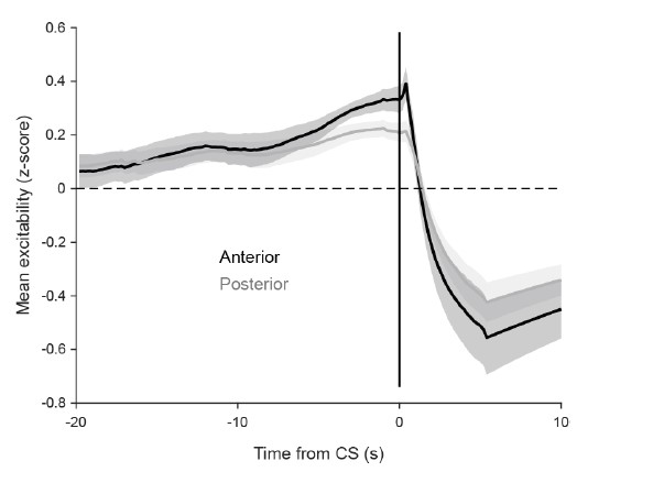
No explanation is given why activity drops ~30 seconds before a convergent saccade (Fig. 7E).
This is no longer shown after we trimmed the history data in Fig 7E in accordance with a comment from reviewer 1. We speculate, however, that the mean linear drive of a compact population of neurons would be somewhat periodical, since a high linear drive leads to a burst which results in a prolonged inhibition (low linear drive) with a slow recovery and so on.
No statistical test is performed on the R^2 distribution (Fig. 7H) to confirm the R^2s (with a mean close to R^2=0.01) are meaningful and not due to random fluctuations.
We revised the analysis in Fig 7 along the same lines as the revision of Fig 4. Model-estimated linear drive predicts CS-associated activity whereas a null estimate (random times) shows no such relationship.
Presentation: A disjointed part of the paper is that for the first part (Figs. 1-3), the focus is on capturing burst activity, but for the second part (Figs. 4-7), the focus is on trial-to-trial variability with no mention of bursts. It is unclear how the reader should relate the two and if bursts serve a purpose for stimulus-evoked activity.
In the first part of the paper (Figs. 1-3), we use ongoing activity to develop an understanding (formulated as a network model) of how activity modulates the network state. In the second part, we test this understanding in the context of evoked responses and show that model-estimated network state explains a fraction of visual response variability and experience-dependent changes in activity and behaviour. In the revised MS we further emphasize this idea and have edited the results text to strengthen the connections between these parts of the study. See also comments above.
Citations: The manuscript may cite other relevant studies in electrophysiology that have investigated noise correlations, such as:
Luczak et al., Neuron 2009 (comparing spontaneous and evoked activity).
Cohen and Kohn, Nat Neuro 2011 (review on noise correlations).
Smith and Kohn, JNeurosci 2008 (looking at correlations over distance).
Lin et al., Neuron 2015 (modeling shared variability).
Goris et al., Nat Neuro 2014 (check out Fig. 4).
Umakantha et al., Neuron 2021 (links noise correlation and dim reduction; includes other recent references to noise correlations).
We agree that the manuscript could benefit from citing some of these suggested studies and have added citations accordingly.
Author Response
Reviewer #1 (Public Review):
In this manuscript, the authors find CpGs within 500Kb of a gene that associate with transcript abundance (cis-eQTMs) in children from the HELIX study. There is much to admire about this work. With two notable exceptions, their work is solid and builds/improves on the work that came before it. Their catalogue of eQTMs could be useful to many other researchers that utilize methylation data from whole blood samples in children. Their annotation of eQTMs is well thought out and exhaustive. As this portion of the work is descriptive, most of their methods are appropriate.
Unfortunately, their use of results from a model that does not account for cell-type proportions across samples diminishes the utility and impact of their findings. I believe that their catalog of eQTMs contains a great deal of spurious results that primarily represent the differences in cell-type proportions across samples.
Lastly, the authors postulate that the eQTM gene associations found uniquely in their unadjusted model (in comparison to results from a model that does account for cell type proportion) represent cell-specific associations that are lost when a fully-adjusted model is assumed. To test this hypothesis, the authors appear to repurpose methods that were not intended for the purposes used in this manuscript. The manuscript lacks adequate statistical validation to support their repurposing of the method, as well as the methodological detail needed to peer review it. This section is a distraction from an otherwise worthy manuscript. But provide evidences that enriched for cell sp CpGs.
Major points
- Line 414-475: In this section, the authors are suggesting that CpGs that are significant without adjusting for cell type are due to methylation-expression associations that are found only in one cell type, while association found in the fully adjusted model are associations that are shared across the cell types. I do not agree with this hypothesis, as I do not agree that the confounding that occurs when cell-type proportions are not accounted for would behave in this way. Although restricting their search for eQTMs to only those CpGs proximal to a gene will reduce the number of spurious associations, a great deal of the findings in the authors' unadjusted model likely reflect differences in cell-type proportions across samples alone. The Reinius manuscript, cited in this paper, indicates that geneproximal CpGs can have methylation patterns that vary across cell types.
Following reviewers’ recommendations, we have reconsidered our initial hypothesis about the role of cellular composition in the association between methylation and gene expression. Although we still think that some of the eQTMs only found in the model unadjusted for cellular composition could represent cell specific effects, we acknowledge that the majority might be confounded by the extensive gene expression and DNA methylation differences between cell types. Also, we recognize that more sophisticated statistical tests should be applied to prove our hypothesis. Because of this, we have decided to report the eQTMs of the model adjusted for cellular composition in the main manuscript and keep the results of the model unadjusted for cellular composition only in the online catalogue.
- Line 476-488: Their evidence due to F-statistics is tenuous. The authors do not give enough methodological detail to explain how they're assessing their hypothesis in the results or methods (lines 932-946) sections. The methods they give are difficult to follow. The results in figure S19A are not compelling. The citation in the methods (by Reinius) do not make sense, because Reinius et al did not use F-statistics as a proxy for cell type specificity. The citation that the authors give for this method in the results does not appear to be appropriate for this analysis, either. Jaffe and Irizarry state that a CpG with a high Fstatistic indicates that the methylation at that CpG varies across cell type. They suggest removing these CpGs from significant results, or estimating and correcting for cell type proportions, as their presence would be evidence of statistical confounding. The authors of this manuscript indicate that they find higher F-statistics among the eQTMs uniquely found in the unadjusted model, which seems to only strengthen the idea that the unadjusted model is suffering from statistical confounding.
We recognize the miss-interpretation of the F-statistic in relation to cellular composition. We have deleted all this part from the updated version of the manuscript.
- The methods used to generate adjusted p-values in this manuscript are not appropriate as they are written. Further, they are nothing like the methods used in the paper cited by the authors. The Bonder paper used permutations to estimate an empirical FDR and cites a publication by Westra et al for their method (below). The Westra paper is a better one to cite, because the methods are more clear. Neither the Bonder nor the Westra paper uses the BH procedure for FDR.
Westra, H.-J. et al. Systematic identification of trans eQTLs as putative drivers of known disease associations. Nat. Genet. 45, 1238-1243 (2013).
We apologize for this misleading citation. Although Bonder et al applied a permutation approach to adjust for multiple testing, our approach was inspired by the method applied in the GTEx project (GTEx consortium, 2020), using CpGs instead of SNPs. The citation has been corrected in the manuscript. Moreover, we have explained in more detail the whole multiple-testing processes in the Material and Methods section (page 14, line 316):
“To ensure that CpGs paired to a higher number of Genes do not have higher chances of being part of an eQTM, multiple-testing was controlled at the CpG level, following a procedure previously applied in the Genotype-Tissue Expression (GTEx) project (Gamazon et al., 2018). Briefly, our statistic used to test the hypothesis that a pair CpGGene is significantly associated is based on considering the lowest p-value observed for a given CpG and all its pairs Gene (e.g. those in the 1 Mb window centered at the TSS). As we do not know the distribution of this statistic under the null, we used a permutation test. We generated 100 permuted gene expression datasets and ran our previous linear regression models obtaining 100 permuted p-values for each CpG-Gene pair. Then, for each CpG, we selected among all CpG-Gene pairs the minimum p-value in each permutation and fitted a beta distribution that is the distribution we obtain when dealing with extreme values (e.g. minimum) (Dudbridge and Gusnanto, 2008). Next, for each CpG, we took the minimum p-value observed in the real data and used the beta distribution to compute the probability of observing a lower p-value. We defined this probability as the empirical p-value of the CpG. Then, we considered as significant those CpGs with empirical p-values to be significant at 5% false discovery rate using BenjaminiHochberg method. Finally, we applied a last step to identify all significant CpG-Gene pairs for all eCpGs. To do so, we defined a genome-wide empirical p-value threshold as the empirical p-value of the eCpG closest to the 5% false discovery rate threshold. We used this empirical p-value to calculate a nominal p-value threshold for each eCpG, based on the beta distribution obtained from the minimum permuted p-values. This nominal p-value threshold was defined as the value for which the inverse cumulative distribution of the beta distribution was equal to the empirical p-value. Then, for each eCpG, we considered as significant all eCpG-Gene variants with a p-value smaller than nominal p-value.”
References:<br /> GTEx consortium, The GTEx Consortium atlas of genetic regulatory effects across human tissues, Science (2020) Sep 11;369(6509):1318-1330. doi: 10.1126/science.aaz1776.
Reviewer #2 (Public Review):
Strength:
Comprehensive analysis Considering genetic factors such as meQTL and comparing results with adult data are interesting.
We thank the reviewer for his/her positive feedback on the manuscript. We agree that the analysis of genetic data and the comparison with eQTMs described in adults are two important points of the study.
Weakness:
- Manuscript is not summarized well. Please send less important findings to supplementary materials. The manuscript is not well written, which includes every little detail in the text, resulting in 86 pages of the manuscript.
Following reviewers’ comments, we have simplified the manuscript. Now only the eQTMs identified in the model adjusted for cellular composition are reported. In addition, functional enrichment analyses have been simplified without reporting all odds ratios (OR) and p-values, which can be seen in the Figures.
- Any possible reason that the eQTM methylation probes are enriched in weak transcription regions? This is surprising.
Bonder et al also found that blood eQTMs were slightly enriched for weak transcription regions (TxWk). Weak transcription regions are highly constitutive and found across many different cell types (Roadmap Epigenetics Consortium, 2015). However, hematopoietic stem cells and immune cells have lower representation of TxWk and other active states, which may be related to their capacity to generate sub-lineages and enter quiescence.
Given that we analyzed whole blood and that ROADMAP chromatin states are only available for blood specific cell types, each CpG in the array was annotated to one or several chromatin states by taking a state as present in that locus if it was described in at least 1 of the 27 bloodrelated cell types. By applying this strategy we may be “over-representing” TxWk chromatin states, in the case TxWk are cell-type specific. As a result, even if each blood cell type might have few TxWk, many positions can be TxWk in at least one cell type, inflating the CpGs considered as TxWk. This might have affected some of the enrichments.
On the other hand, CpG probe reliability depends on methylation levels and variance. TxWk regions show high methylation levels, which tend to be measured with more error. This also might have impacted the results, however the analysis considering only reliable probes (ICC >0.4) showed similar enrichment for TxWk.
Besides these, we do not have a clear answer for the question raised by the reviewer.
References:
Bonder MJ, Luijk R, Zhernakova D V, Moed M, Deelen P, Vermaat M, et al. Disease variants alter transcription factor levels and methylation of their binding sites. Nat Genet [Internet]. 2017 [cited 2017 Nov 2];49:131–8. Available from: http://www.ncbi.nlm.nih.gov/pubmed/27918535
Roadmap Epigenomics Consortium, Kundaje A, Meuleman W, Ernst J, Bilenky M, Yen A, Heravi-Moussavi A, Kheradpour P, Zhang Z, Wang J, Ziller MJ, Amin V, Whitaker JW, Schultz MD, Ward LD, Sarkar A, Quon G, Sandstrom RS, Eaton ML, Wu YC, Pfenning AR, Wang X, Claussnitzer M, Liu Y, Coarfa C, Harris RA, Shoresh N, Epstein CB, Gjoneska E, Leung D, Xie W, Hawkins RD, Lister R, Hong C, Gascard P, Mungall AJ, Moore R, Chuah E, Tam A, Canfield TK, Hansen RS, Kaul R, Sabo PJ, Bansal MS, Carles A, Dixon JR, Farh KH, Feizi S, Karlic R, Kim AR, Kulkarni A, Li D, Lowdon R, Elliott G, Mercer TR, Neph SJ, Onuchic V, Polak P, Rajagopal N, Ray P, Sallari RC, Siebenthall KT, Sinnott-Armstrong NA, Stevens M, Thurman RE, Wu J, Zhang B, Zhou X, Beaudet AE, Boyer LA, De Jager PL, Farnham PJ, Fisher SJ, Haussler D, Jones SJ, Li W, Marra MA, McManus MT, Sunyaev S, Thomson JA, Tlsty TD, Tsai LH, Wang W, Waterland RA, Zhang MQ, Chadwick LH, Bernstein BE, Costello JF, Ecker JR, Hirst M, Meissner A, Milosavljevic A, Ren B, Stamatoyannopoulos JA, Wang T, Kellis M. Integrative analysis of 111 reference human epigenomes. Nature. 2015 Feb 19;518(7539):317-30. doi: 10.1038/nature14248. PMID: 25693563; PMCID: PMC4530010.
- The result that the magnitude of the effect was independent of the distance between the CpG and the TC TSS is surprising. Could you draw a figure where x-axis is the distance between the CpG site and TC TSS and y-axis is p-value?
As suggested by the reviewer, we have taken a more detailed look at the relationship between the effect size and the distance between the CpG and the TC’s TSS. First, we confirmed that the relative orientation (upstream or downstream) did not affect the strength of the association (p-value=0.68). Second, we applied a linear regression between the absolute log2 fold change and the log10 of the distance (in absolute value), finding that they were inversely related. We have updated the manuscript with this information (page 22, line 504):
“We observed an inverse linear association between the eCpG-eGene’s TSS distance and the effect size (p-value = 7.75e-9, Figure 2B); while we did not observe significant differences in effect size due to the relative orientation of the eCpG (upstream or downstream) with respect to the eGene’s TSS (p-value = 0.68).”
Results are shown in Figure 2B. Of note, we winsorized effect size values in order to improve the visualization. The winsorizing process is also explained in Figure 2 legend. Moreover, we have done the plot suggested by the reviewer (see below). It shows that associations with smallest p-values are found close to the TC’s TSS. Nonetheless, as this pattern is also observed for the effect sizes, we have decided to not include it in the manuscript.
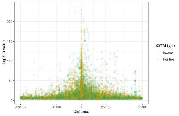
- Concerned about too many significant eQTMs. Almost half of genes are associated with methylation. I wonder if false positives are well controlled using the empirical p-values. Using empirical p-value with permutation may mislead since especially you only use 100 permutations. I wonder the result would be similar if they compare their result with the traditional way, either adjusting p-values using p-values from entire TCs or adjusting pvalues using a gene-based method as commonly used in GWAS. Compare your previous result with my suggestion for the first analysis.
Despite the number of genes (TCs) whose expression is associated with DNA methylation is quite high, we do not think this is due to not correctly controlling false positives. Our approach is based on the method used by GTEx (GTEx consortium) and implemented in the FastQTL package (Ongen et al. 2016), to control for positives in the eQTLs discovery. As in GTEx, we run 100 permutations to estimate the parameters of a beta distribution, which we used to model the distribution of p-values for each CpG. Then, to correct for the number of TCs among significant CpGs, we applied False Discovery Rate (FDR) at a threshold < 0.05. Finally, we defined the final set of significant eQTMs using the beta distribution defined in a previous step.
For illustration, we compared the number of eQTMs with our approach to what we would obtain by uniquely applying the FDR method (adjusted p-value <0.05), getting fewer associations with our approach: eQTMs (45,203 with FDR vs 39,749 with our approach), eCpGs (24,611 vs 21,966) and eGenes (9,937 vs 8,886). Among the 8,886 significant eGenes, 6,288 of them are annotated to coding genes, thus representing 27% of the 23,054 eGenes coding for a gene included in the array.
References:
GTEx consortium, The GTEx Consortium atlas of genetic regulatory effects across human tissues, Science (2020) Sep 11;369(6509):1318-1330. doi: 10.1126/science.aaz1776.
Ongen et al. Fast and efficient QTL mapper for thousands of molecular phenotypes, Bioinformatics (2016) May 15;32(10):1479-85. doi: 10.1093/bioinformatics/btv722. Epub 2015 Dec 26.
- I recommend starting with cell type specific results. Without adjusting cell type, the result doesn't make sense.
As suggested by other reviewers, we have withdrawn the model unadjusted for cellular composition.
Reviewer #3 (Public Review):
Although several DNA methylation-gene expression studies have been carried out in adults, this is the first in children. The importance of this is underlined by the finding that surprisingly few associations are observed in both adults and children. This is a timely study and certain to be important for the interpretation of future omic studies in blood samples obtained from children.
We agree with the reviewer that eQTMs in children are important for interpreting EWAS findings conducted in child cohorts such as those of the Pregnancy And Childhood Epigenetics (PACE) consortium.
It is unfortunate that the authors chose to base their reporting on associations unadjusted for cell count heterogeneity. They incorrectly claim that associations linked to cell count variation are likely to be cell-type-specific. While possible, it is probably more likely that the association exists entirely due to cell type differences (which tend to be large) with little or no association within any of the cell types (which tend to be much smaller). In the interests of interpretability, it would be better to report only associations obtained after adjusting for cell count variation.
Following reviewers’ recommendations, we have reconsidered our initial hypothesis about the role of cellular composition in the association between methylation and gene expression. Although we still think that some of the eQTMs only found in the model unadjusted for cellular composition could represent cell specific effects, we acknowledge that the majority might be confounded by the extensive gene expression and DNA methylation differences between cell types. Also, we recognize that more sophisticated statistical tests should be applied to prove our hypothesis. Because of this we have decided to report the eQTMs of the model adjusted for cellular composition in the main manuscript and keep the results of the model unadjusted for cellular composition only in the online catalogue.
Several enrichments could be related to variation in probe quality across the DNA methylation arrays.
For example, enrichment for eQTM CpG sites among those that change with age could simply be due to the fact age and eQTM effects are more likely to be observed for CpG sites with high quality probes than low quality probes. It is more informative to instead ask if eQTM CpG sites are more likely to have increasing rather than decreasing methylation with age. This avoids the probe quality bias since probes with positive associations with age would be expected to have roughly the same quality as those with negative associations with age. There are several other analyses prone to the probe quality bias.
See answer to question 2, below.
Author Response:
Reviewer #1:
This work provides insight into the effects of tetraplegia on the cortical representation of the body in S1. By using fMRI and an attempted finger movement task, the researchers were able to show preserved fine-grained digit maps - even in patients without sensory and motor hand function as well as no spared spinal tissue bridges. The authors also explored whether certain clinical and behavioral determinates may contribute to preserving S1 somatotopy after spinal cord injury.
Overall I found the manuscript to be well-written, the study to be interesting, and the analysis reasonable. I do, however, think the manuscript would benefit by considering and addressing two main suggestions.
1) Provide additional context / rationale for some of the methods. Specific examples below:
a) The rationale behind using the RSA analysis seemed to be predicated on the notion that the signals elicited via a phase-encoded design can only yield information about each voxel's preferred digit and little-to-no information about the degree of digit overlap (see lines 163-166 and 571-575). While this is the case for conventional analyses of these signals, there are more recently developed approaches that are now capable of estimating the degree of somatotopic overlap from phase-encoded data (see: Da Rocha Amaral et al., 2020; Puckett et al., 2020). Although I personally would be interested in seeing one of these types of analyses run on this data, I do not think it is necessary given the RSA data / analysis. Rather, I merely think it is important to add some context so that the reader is not misled into believing that there is no way to estimate this type of information from phase-encoded signals. - Da Rocha Amaral S, Sanchez Panchuelo RM, Francis S (2020) A Data-Driven Multi-scale Technique for fMRI Mapping of the Human Somatosensory Cortex. Brain Topogr 33 (1):22-36. doi:10.1007/s10548-019-00728-6 - Puckett AM, Bollmann S, Junday K, Barth M, Cunnington R (2020) Bayesian population receptive field modeling in human somatosensory cortex. Neuroimage 208:116465. doi:10.1016/j.neuroimage.2019.116465
We did not intend to give the impression that inter-finger overlap can only be estimated using RSA. To clarify this, we included a sentence in our methods section stating that inter-finger overlap cannot be estimated using the traditional travelling wave approach, but new methods have estimated somatotopic overlap from travelling wave data. Since our RSA approach lends itself for estimating inter-finger overlap and is currently the gold standard in characterizing these representational patterns, we opt –in accordance with the reviewer’s comment– not to include this additional analysis.
Revised text Methods:
“While the traditional traveling wave approach is powerful to uncover the somatotopic finger arrangement, a fuller description of hand representation can be obtained by taking into account the entire fine-grained activity pattern of all fingers. RSA-based inter-finger overlap patterns have been shown to depict the invariant representational structure of fingers better than the size, shape, and exact location of the areas activated by finger movements (Ejaz et al., 2015). RSA-based measures are furthermore not prone to some of the problems of measurements of finger selectivity (e.g., dependence on map thresholds). The most common approach for investigating inter-finger overlap is RSA, as used here, though note that somatotopic overlap has recently been estimated from travelling wave data using an iterated Multigrid Priors (iMGP) method and population receptive field modelling (Da Rocha Amaral et al., 2020; Puckett et al., 2020).”
b. The rationale for using minimally thresholded (Z>2) data for the Dice overlap analysis as opposed to the threshold used in data visualization (q<0.05) was unclear. Providing the minimally thresholded maps (in Supplementary) would also aid interpretation of the Dice overlap results.
We followed previously published procedures for calculating the Dice overlap between the two split-halves of the data (Kikkert et al., 2016; J. Kolasinski et al., 2016; Sanders et al., 2019). We used minimally thresholded data to calculate the dice overlap to ensure that our analysis was sensitive to overlaps that would be missed when using high thresholds. We clarified this in the revised manuscript. We thank the reviewer for their suggestion to add a Figure displaying the minimally thresholded split-half hard-edged finger maps - we have added this to the revised manuscript as Figure 2-Figure supplement 1.
To ensure that our thresholding procedure did not change the results of the dice overlap analysis, we repeated this analysis using split-half maps that were thresholded using a q < 0.05 FDR criterion (as was used to create the travelling wave maps in Figures 2A-B). We found the same results as when using the Z >2 thresholding criterion: Overall, split-half consistency was not significantly different between patients and controls, as tested using a robust mixed ANOVA (F(1,17.69) = 0.08, p = 0.79). There was a significant difference in split- half consistency between pairs of same, neighbouring, and non-neighbouring fingers (F(2,14.77) = 38.80, p < 0.001). This neighbourhood relationship was not significantly different between the control and patient groups (i.e., there was no significant interaction; F(2,14.77) = 0.12, p = 0.89). We have included this analysis and the relating figure as Figure 2- Figure supplement 2 in the revised manuscript.
Revised text Methods:
“We followed previously described procedures for calculating the DOC between two halves of the travelling wave data (Kikkert et al., 2016; Kolasinski et al., 2016; Sanders et al., 2019). The averaged finger-specific maps of the first forward and backward runs formed the first data half. The averaged finger-specific maps of the second forward and backward runs formed the second data half. The finger-specific clusters were minimally thresholded (Z>2) on the cortical surface and masked using an S1 ROI, created based on Brodmann area parcellation using Freesurfer (see Figure 2– figure supplement 1 for a visualisation of the minimally thresholded split-half hard-edged finger maps used to calculate the DOC). We used minimally thresholded finger-specific clusters for the DOC analysis to ensure we were sensitive to overlaps that would be missed when using high thresholds. Note that results were unchanged when thresholding the finger-specific clusters using an FDR q < 0.05 criterion (see Figure 2 – figure supplement 2).”
2) Provide a more thorough discussion - particularly with respect to the possible role of top-down processes (e.g., attention).
a) The authors discuss a few potential signal sources that may contribute to the maintenance of (and ability to measure) the somatotopic maps; however, the overall interpretation seems a bit "motor efferent heavy". That is, it seems the authors favor an explanation that the activity patterns measured in S1 were elicited by efference copies from the motor system and that occasional corollary discharges or attempted motor movements play a role in their maintenance over time. The authors consider other explanations, noting - for example - the potential role of attention in preserving the somatotopic representations given that attention has been shown to be able to activate S1 hand representations. The mention of this was, however, rather brief - and I believe the issue deserves a bit more of a balanced consideration.
When the authors consider the possible role of attention in maintaining the somatotopic representations (lines 329-333), they mention that observing others' fingers being touched or attending to others' finger movements may contribute. But there is no mention of attending to one's own fingers (which has been shown to elicit activity as cited). I realize that the patients lack sensorimotor function (and hence may find it difficult to "attend" to their fingers); however, they have all had prior experience with their fingers and therefore might still be able to attend to them (or at least the idea of their digits) such that activity is elicited. For example, it is not clear to me that it would be any more difficult for the patients to be asked to attend to their digits compared to being asked to attempt to move their digits. I would even suggest that attempting to move a digit (regardless of whether you can or not) requires that one attends to the digit before attempting to initiate the movement as well as throughout the attempted motor movement. Because of this, it seems possible that attention-related processes could be playing a role in or even driving the signals measured during the attempted movement task - as well as those involved in the ongoing maintenance of the maps after injury. I don't think this possibility can be dismissed given the data in hand, but perhaps the issue could be addressed by a bit more thorough of a discussion on the process of "attempting to move" a digit (even one that does not move) - and the various top-down processes that might be involved.
We thank the reviewer for their consideration and insights into the potential mechanisms underlying our results. We have now elaborated further on the possibility that attention- related processes might have contributed to the reported effects, also in consideration of comment 3.4.
Revised text Discussion:
“Spared spinal cord tissue bridges can be found in most patients with a clinically incomplete injury, their width being predictive of electrophysiological information flow, recovery of sensorimotor function, and neuropathic pain (Huber et al., 2017; Pfyffer et al., 2021, 2019; Vallotton et al., 2019). However, in this study, spared midsagittal spinal tissue bridges at the lesion level, motor function, and sensory function did not seem necessary to maintain and activate a somatotopic hand representation in S1. We found a highly typical hand representation in two patients (S01 and S03) who did not have any spared spinal tissue bridges at the lesion level, a complete (S01) or near complete (S03) hand paralysis, and a complete (S01) or near complete loss (S03) of hand sensory function. Our predictive modelling results were in line with this notion and showed that these behavioural and structural spinal cord determinants were not predictive of hand representation typicality. Note however that our sample size was limited, and it is challenging to draw definite conclusions from non-significant predictive modelling results.”
“How may these representations be preserved over time and activated through attempted movements in the absence of peripheral information? S1 is reciprocally connected with various brain areas, e.g., M1, lateral parietal cortex, poster parietal area 5, secondary somatosensory cortex, and supplementary motor cortex (Delhaye et al., 2019). After loss of sensory inputs and paralysis through SCI, S1 representations may be activated and preserved through its interconnections with these areas. Firstly, it is possible that cortico-cortical efference copies may keep a representation ‘alive’ through occasional corollary discharge (London and Miller, 2013). While motor and sensory signals no longer pass through the spinal cord in the absence of spinal tissue bridges, S1 and M1 remain intact. When a motor command is initiated (e.g., in the form of an attempted hand movement) an efference copy is thought to be sent to S1 in the form of corollary discharge. This corollary discharge resembles the expected somatosensory feedback activity pattern and may drive somatotopic S1 activity even in the absence of ascending afferent signals from the hand (Adams et al., 2013; London and Miller, 2013). It is possible that our patients occasionally performed attempted movements which would result in corollary discharge in S1. Second, it is likely that attempting individual finger movements poses high attentional demands on tetraplegic patients. Accordingly, attentional processes might have contributed to eliciting somatotopic S1 activity. Evidence for this account comes from studies showing that it is possible to activate somatotopic S1 hand representations through attending to individual fingers (Puckett et al., 2017) or through touch observation (Kuehn et al., 2018). Attending to fingers during our attempted finger movement task may have been sufficient to elicit somatotopic S1 activity through top-down processes in the tetraplegic patients who lacked hand motor and sensory function. Furthermore, one might speculate that observing others’ or one’s own fingers being touched or directing attention to others’ hand movements or one’s own fingers may help preserve somatotopic representations. Third, it is possible that these somatotopic maps are relatively hardwired and while they deteriorate over time, they never fully disappear. Indeed, somatotopic mapping of a sensory deprived body part has been shown to be resilient after dystonia (Ejaz et al., 2016; though see Burman et al., (2009) and Taub et al., (1998)) and arm amputation (Bruurmijn et al., 2017; Kikkert et al., 2016; Wesselink et al., 2019). Fourth, it is possible that even though a patient is clinically assessed to be complete and is unable to perceive sensory stimuli on the deprived body part, there is still some ascending information flow that contributes to preserving somatotopy (Wrigley et al., 2018). A recent study found that although complete paraplegic SCI patients were unable to perceive a brushing stimulus on their toe, 48% of patients activated the location appropriate S1 area (Wrigley et al., 2018). However, the authors of this study defined the completeness of patients’ injuries via behavioural testing, while we additionally assessed the retained connections passing through the SCI directly via quantification of spared spinal tissue bridges through structural MRI. It is unlikely that spinal tissue carrying somatotopically organised information would be missed by our assessment (Huber et al., 2017; Pfyffer et al., 2019). Our experiment did not allow us to tease apart these potential processes and it is likely that various processes simultaneously influence the preservation of S1 somatotopy and elicited the observed somatotopic S1 activity.”
Reviewer #2:
The authors investigate SCI patients and characterize the topographic representation of the hand in sensorimotor cortex when asked to move their hand (which controls could do but patients could not). The authors compare some parameters of topographic map organization and conclude that they do not differ between patients and controls, whereas they find changes in the typicality of the maps that decrease with years since disease onset in patients. Whereas these initial analyses are interesting, they are not clearly related to a mechanistic model of the disorder and the underlying pathophysiology that is expected in the patients. Furthermore, additional analyses on more fine-grained map changes are needed to support the authors' claims. Finally, the major result of changed typicality in the patients is in my view not valid.
- Concept 1. At present, there is no clear hypotheses about the (expected or hypothesized) mechanistic changes of the sensorimotor maps in the patients. The authors refer to "altered" maps and repeatedly say that "results are mixed" (3 times in the introduction).
We thank the reviewer for highlighting to us that our introduction and hypotheses were unclear and/or incomplete to them. We have restructured our Introduction to better highlight competing hypotheses on how SCI may change S1 hand representations, the reasons for our analytical approach, and elaborate on our hypotheses.
Revised text Introduction:
“Research in non-human primate models of chronic and complete cervical SCI has shown that the S1 hand area becomes largely unresponsive to tactile hand stimulation after the injury (Jain et al., 2008; Kambi et al., 2014; Liao et al., 2021). The surviving finger-related activity became disorganised such that a few somatotopically appropriate sites but also other somatotopically nonmatched sites were activated (Liao et al., 2021). Seminal nonhuman primate research has further demonstrated that SCI leads to extensive cortical reorganisation in S1, such that tactile stimulation of cortically adjacent body parts (e.g., of the face) activated the deprived brain territory (e.g., of the hand; Halder et al., 2018; Jain et al., 2008; Kambi et al., 2014). Although the physiological hand representation appears to largely be altered following a chronic cervical SCI in non-human primates, the anatomical isomorphs of individual fingers are unchanged (Jain et al., 1998). This suggests that while a hand representation can no longer be activated through tactile stimulation after the loss of afferent spinal pathways, a latent and somatotopic hand representation could be preserved regardless of large-scale physiological reorganisation.
A similar pattern of results has been reported for human SCI patients. Transcranial magnetic stimulation (TMS) studies induced current in localised areas of SCI patient’s M1 to induce a peripheral muscle response. They found that representations of more impaired muscles retract or are absent while representations of less impaired muscles shift and expand (Fassett et al., 2018; Freund et al., 2011a; Levy et al., 1990; Streletz et al., 1995; Topka et al., 1991; Urbin et al., 2019). Similarly, human fMRI studies have shown that cortically neighbouring body part representations can shift towards, though do not invade, the deprived M1 and S1 cortex (Freund et al., 2011b; Henderson et al., 2011; Jutzeler et al., 2015; Wrigley et al., 2018, 2009). Other human fMRI studies hint at the possibility of latent somatotopic hand representations following SCI by showing that attempted movements with the paralysed and sensory deprived body part can still evoke signals in the sensorimotor system (Cramer et al., 2005; Freund et al., 2011b; Kokotilo et al., 2009; Solstrand Dahlberg et al., 2018). This attempted ‘net’ movement activity was, however, shown to substantially differ from healthy controls: Activity levels have been shown to be increased (Freund et al., 2011b; Kokotilo et al., 2009; Solstrand Dahlberg et al., 2018) or decreased (Hotz- Boendermaker et al., 2008), volumes of activation have been shown to be reduced (Cramer et al., 2005; Hotz-Boendermaker et al., 2008), activation was found in somatotopically nonmatched cortical sites (Freund et al., 2011b), and activation was poorly modulated when patients switched from attempted to imagined movements (Cramer et al., 2005). These observations have therefore mostly been attributed to abnormal and/or disorganised processing induced by the SCI. It remains possible though that, despite certain aspects of sensorimotor activity being altered after SCI, somatotopically typical representations of the paralysed and sensory deprived body parts can be preserved (e.g., finger somatotopy of affected hand). Such preserved representations have the potential to be exploited in a functionally meaningful manner (e.g., via neuroprosthetics).
Case studies using intracortical stimulation in the S1 hand area to elicit finger sensations in SCI patients hint at such preserved somatotopic representations (Fifer et al., 2020; Flesher et al., 2016), with one exception (Armenta Salas et al., 2018). Negative results were suggested to be due to a loss of hand somatotopy and/or reorganisation in S1 of the implanted SCI patient or due to potential misplacement of the implant (Armenta Salas et al., 2018). Whether fine-grained somatotopy is generally preserved in the tetraplegic patient population remains unknown. It is also unclear what clinical, behavioural, and structural spinal cord determinants may influence such representations to be maintained. Here we used functional MRI (fMRI) and a visually cued (attempted) finger movement task in tetraplegic patients to examine whether hand somatotopy is preserved following a disconnection between the brain and the periphery. We instructed patients to perform the fMRI tasks with their most impaired upper limb and matched controls’ tested hands to patients’ tested hands. If a patient was unable to make overt finger movements due to their injury, then we carefully instructed them to make attempted (i.e., not imagined) finger movements. To see whether patient’s maps exhibited characteristics of somatotopy, we visualised finger selectivity in S1 using a travelling wave approach. To investigate whether fine-grained hand somatotopy was preserved and could be activated in S1 following SCI, we assessed inter-finger representational distance patterns using representational similarity analysis (RSA). These inter-finger distance patterns are thought to be shaped by daily life experience such that fingers used more frequently together in daily life have lower representational distances (Ejaz et al., 2015). RSA-based inter-finger distance patterns have been shown to depict the invariant representational structure of fingers in S1 and M1 better than the size, shape, and exact location of the areas activated by finger movements (Ejaz et al., 2015). Over the past years RSA has therefore regularly been used to investigate somatotopy of finger representations both in healthy (e.g., Akselrod et al., 2017; Ariani et al., 2020; Ejaz et al., 2015; Gooijers et al., 2021; Kieliba et al., 2021; Kolasinski et al., 2016; Liu et al., 2021; Sanders et al., 2019) and patient populations (e.g., Dempsey-Jones et al., 2019; Ejaz et al., 2016; Kikkert et al., 2016; Wesselink et al., 2019). We closely followed procedures that have previously been used to map preserved and typical somatotopic finger selectivity and inter-finger representational distance patterns of amputees’ missing hands in S1 using volitional phantom finger movements (Kikkert et al., 2016; Wesselink et al., 2019). However, in amputees, these movements generally recruit the residual arm muscles that used to control the missing limb via intact connections between the brain and spinal cord. Whether similar preserved somatotopic mapping can be observed in SCI patients with diminished or no connections between the brain and the periphery is unclear. If finger somatotopy is preserved in tetraplegic patients, then we should find typical inter-finger representational distance patterns in the S1 hand area of these patients. By measuring a group of fourteen chronic tetraplegic patients with varying amounts of spared spinal cord tissue at the lesion level (quantified by means of midsagittal tissue bridges based on sagittal T2w scans), we uniquely assessed whether preserved connections between the brain and periphery are necessary to preserve fine somatotopic mapping in S1 (Huber et al., 2017; Pfyffer et al., 2019). If spared connections between the periphery and the brain are not necessary for preserving hand somatotopy, then we would find typical inter-finger representational distance patterns even in patients without spared spinal tissue bridges. We also investigated what clinical and behavioural determinants may contribute to preserving S1 hand somatotopy after chronic SCI. If spared sensorimotor hand function is not necessary for preserving hand somatotopy, then we would find typical inter-finger representational distance patterns even in patients who suffer from full sensory loss and paralysis of the hand(s).”
They do not in detail report which results actually have been reported before, which is a major problem, because those prior results should have motivated the analyses the authors conducted. For instance, two of the cited studies found that in SCI patients, only ONE FINGER shifted towards the malfunctioning area (i.e., the small finger) whereas all other fingers were the same. However, the authors do NOT perform single finger analyses but always average their results ACROSS fingers. This is even true in spite of some patients indeed showing MISSING FINGERS as is clearly evident in the figure, and in spite of the clearly reduced distance of the thumb in the patients as is also visible in another figure. Nothing of this is seen in the results, because the ANOVA and analyses never have the factor of "finger". Instead, the authors always average the analyses across finger. The conclusion that the maps do not differ is therefore not justified at present. This severely reduces any conclusions that an be drawn from the data at present.
We apologise for the lack of clarity. We now added additional detail regarding studies showing altered sensorimotor processing following SCI. We also clarified that we based our analysis steps on previous studies investigating hand somatotopy following deafferentation (i.e., following arm amputation; Kikkert et al., 2016; Wesselink et al., 2019) and somatotopic reorganisation RSA- based inter-finger distance patterns have been shown to depict the invariant representational structure of fingers in S1 and M1 better than the size, shape, and exact location of the areas activated by finger movements (Ejaz et al., 2015). Over the past years RSA has therefore regularly been used to investigate somatotopy of finger representations both in healthy (e.g., Akselrod et al., 2017; Ariani et al., 2020; Ejaz et al., 2015; Gooijers et al., 2021; Kieliba et al., 2021; Kolasinski et al., 2016; Liu et al., 2021; Sanders et al., 2019) and patient populations (e.g. Dempsey-Jones et al., 2019; Ejaz et al., 2016; Kikkert et al., 2016; Wesselink et al., 2019). It is believed to be the most appropriate measure to reliably detect subtle changes in somatotopy. We adjusted the text in our revised Introduction section to better highlight this.
Please note that we do not average across fingers in our RSA typicality procedure. Instead, RSA considers how the (attempted) movement with one finger changes the activity pattern across the whole hand representation. Note that somatotopic reorganisation will change the inter-finger distance measured with this method as previously shown (Kieliba et al., 2021; Kolasinski et al., 2016; Wesselink et al., 2019).
Still, as per the reviewer’s suggestion, we conducted a robust mixed ANOVA on the RSA distance measures with a within-subjects factor for finger pair (10 levels) and a between- subjects factor for group (2 levels: controls and SCI patients). We did not find a significant group effect (F(1,21.66) = 1.50, p = 0.23). There was a significant difference in distance between finger pairs (F(9,15.38) = 27.22, p < 0.001), but this was not significantly different between groups (i.e., no significant finger pair by group interaction; F(9,15.38) = 1.05, p = 0.45). When testing for group differences per finger pair, the BF only revealed inconclusive evidence (BF > 0.37 and < 1.11; note that we could not run a Bayesian ANOVA due to normality violations). We have added this analysis to the revised manuscript.
Lastly, we would like to highlight that our argument is that the finger maps can be preserved in the absence of sensory and motor function, but over time they deteriorate and become less somatotopic. As such, we do not aim to state that they are unchanged overall – but rather that they can be unchanged even despite loss of sensory and motor function. We have clarified this in our abstract and manuscript to avoid confusion.
Revised abstract:
“Previous studies showed reorganised and/or altered activity in the primary sensorimotor cortex after a spinal cord injury (SCI), suggested to reflect abnormal processing. However,little is knownaboutwhether somatotopically-specific representations can be preserved despite alterations in net activity. In this observational study we used functional MRI and an (attempted) finger movement task in tetraplegic patients to characterise the somatotopic hand layout in primary somatosensory cortex. We further used structural MRI to assess spared spinal tissue bridges. We found that somatotopic hand representations can be preserved in absence of sensory and motor hand functioning, and no spared spinal tissue bridges. Such preserved hand somatotopy could be exploited by rehabilitation approaches that aim to establish new hand-brain functional connections after SCI (e.g., neuroprosthetics). However, over years since SCI the hand representation somatotopy deteriorated, suggesting that somatotopic hand representations are more easily targeted within the first years after SCI.”
Revised text Methods:
“Second, we tested whether the inter-finger distances were different between controls and patients using a robust mixed ANOVA with a within-participants factor for finger pair (10 levels) and a between-participants factor for group (2 levels: controls and patients).”
Revised text Results:
“We then tested whether the inter-finger distances were different across finger pairs between controls and SCI patients using a robust mixed ANOVA with a within-participants factor for finger pair (10 levels) and a between-participants factor for group (2 levels: controls and patients). We did not find a significant difference in inter-finger distances between patients and controls (F(1,21.66) = 1.50, p = 0.23). The inter-finger distances were significantly different across finger pairs, as would be expected based on somatotopic mapping (F(9,15.38) = 27.22, p < 0.001). This pattern of inter-finger distances was not significantly different between groups (i.e., no significant finger pair by group interaction; F(9,15.38) = 1.05, p = 0.45). When testing for group differences per finger pair, the BF only revealed inconclusive evidence (BF > 0.37 and < 1.11; note that we could not run a Bayesian ANOVA due to normality violations).”
Revised text Discussion:
“In this study we investigated whether hand somatotopy is preserved and can be activated through attempted movements following tetraplegia. We tested a heterogenous group of SCI patients to examine what clinical, behavioural, and structural spinal cord determinants contribute to preserving S1 somatotopy. Our results revealed that detailed hand somatotopy can be preserved following tetraplegia, even in the absence of sensory and motor function and a lack of spared spinal tissue bridges. However, over time since SCI these finger maps deteriorated such that the hand somatotopy became less typical.”
- Concept 2: This also relates to the fact that the most prominent and consistent finding of prior studies was to show changes in map AMPLITUDE in the maps of patients. It is not clear to me how amplitude was measured here, because the text says "average BOLD activity". What should be reported are standard measures of signal amplitude both across the map area and for individual fingers.
We apologise for the lack of clarity, “average BOLD activity” represented the average z- standardised activity within the S1 hand ROI. To comply with the reviewer’s comment, we adjusted this to the percent signal change underneath the S1 hand ROI and report this instead in our revised manuscript and in revised Figure 3A and revised Figure 3- Figure supplement 1. Note that results were unchanged.
As per the reviewer’s suggestion, we further extracted the activity levels for individual fingers under finger-specific ROIs. To create finger-specific ROIs, probability finger maps were created based on the travelling wave data of the control group, thresholded at 25% (i.e., meaning that at least 5 out of 18 control participants needed to significantly activate a vertex for this vertex to be included in the ROI), and binarised. We then used the separately acquired blocked design data to extract the corresponding finger movement activity levels underlying these finger-specific ROIs per participant. Per ROI, we then compared the activity level between groups. After correction for multiple comparisons, there was no significant difference between groups for the thumb (U = 93, p = 0.37), index (t(30) = -0.003, p = 0.99), middle (t(30) = 1.11, p = 0.35), ring (t(30) = 2.02, p = 0.13), or little finger (t(30) = 2.14, p = 0.20). We have added this analysis to Appendix 1.
Note that lower or higher BOLD amplitude levels do not influence our typicality scores per se. Indeed, typical inter-finger representational patterns have been shown to persist even in ipsilateral M1 that exhibited a negative BOLD response during finger movements (Berlot et al., 2019). As long as the typical inter-finger relationships are preserved, brain areas that have low amplitudes of activity can have a typical somatotopic representation.
Revised text in Methods:
"The percent signal change for overall task-related activity was then extracted for voxels underlying this S1 hand ROI per participant. A similar analysis was used to investigate overall task-related activity in an M1 hand ROI (see Figure 3- Figure supplement 1). We further compared activity levels in finger-specific ROIs in S1 between groups and conducted a geodesic distance analysis to assess whether the finger representations of the SCI patients were aligned differently and/or shifted compared to the control participants (see Appendix 1)."
Revised text in Results:
“Task-related activity was quantified by extracting the percent signal change for finger movement (across all fingers) versus baseline across within the contralateral S1 hand ROI (see Figure 3A). Overall, all patients were able to engage their S1 hand area by moving individual fingers (t(13)=7.46, p < 0.001; BF10=4.28e +3), as did controls (t(17)=9.92, p < 0.001; BF10=7.40e +5). Furthermore, patients’ task-related activity was not significantly different from controls (t(30)=-0.82, p=0.42; BF10=0.44), with the BF showing anecdotal evidence in favour of the null hypothesis.”
Revised Appendix 1:
“Percent signal change in finger-specific clusters To assess whether finger movement activity levels were different between patients and controls, we created finger-specific ROIs and extracted the activity level of the corresponding finger movement for each participant. To create the finger-specific ROIs, the probability finger surface maps that were created from the travelling wave data of the control group (see main manuscript) were thresholded at 25% (i.e., meaning that at least 5 out of 18 control participants needed to significantly activate a vertex for this vertex to be included in the ROI), and binarised. We then used the separately acquired blocked design data to extract the finger movement activity levels underlying these finger-specific ROIs. We first flipped the contrast images resulting from each participant’s fixed effects analysis (i.e., that was ran to average across the 4 blocked design runs) along the x-axis for the left-hand tested participants. Each participant’s contrast maps were then resampled to the Freesurfer 2D average atlas and the averaged z-standardised activity level was extracted for each finger movement vs rest contrast underlying the finger-specific ROIs. We compared the activity levels for each finger movement in the corresponding finger ROI (i.e., thumb movement activity in the thumb ROI, index finger movement activity in the index finger ROI, etc.) between groups. After correction for multiple comparisons, there was no significant difference between groups for the thumb (U = 93, p = 0.37), index (t(30) = -0.003, p = 0.99), middle (t(30) = 1.11, p = 0.35), ring (t(30) = 2.02, p = 0.13), or little finger (t(30) = 2.14, p = 0.20).”
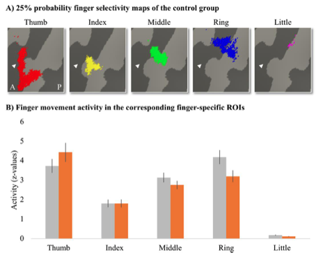
Appendix 1- Figure 1: Finger-specific activity levels in finger-specific regions of interest. A) Finger- specific ROIs were based on the control group’s binarised 25% probability travelling wave finger selectivity maps. B) Finger movement activity levels in the corresponding finger-specific ROIs. There were no significant differences in activity levels between the SCI patient and control groups. Controls are projected in grey; SCI patients are projected in orange. Error bars show the standard error of the mean. White arrows indicate the central sulcus. A = anterior; P = posterior.
- Concept 3: The authors present a hypothesis on the underlying mechanisms of SCI that does not seem to reflect prior data. The argument is that changes in map alignment relate to maladaptive changes and pain. However, the literature that the authors cite does not support this claim. In fact, Freund 2011 promotes the importance of map amplitude but not alignment, whereas other studies either show no relation of activation to pain, or they even show that map shift relates to LESS pain, i.e., the reverse argument than what the authors say. My impression is that the model that the authors present is mainly a model that is used for phantom pain but not for SCI. Taking this into consideration, the findings the authors present are not surprising anymore, because in fact none of these studies claimed that the affected area should be absent in SCI patients; these papers only say that the other body parts change in location or amplitude, which is something the authors did not measure. It is important to make this clear in the text.
As the reviewer states, the literature is debated regarding the relationship between reorganisation and pain in SCI patients. We did not highlight this clearly enough. To improve clarity and focus our message we have therefore removed the sentence regarding reorganisation and pain from the Introduction of our revised manuscript. Also taking comment 2.1 and 2.2 into consideration, we have restructured our Introduction.
We respectfully disagree with the reviewer that our results are not novel or surprising. Whether the full fine-grained hand somatotopy is preserved following a complete motor and sensory loss through tetraplegia has not been considered before. Furthermore, to our knowledge, there is no paper that has inspected the full somatotopic layout in a heterogenous sample of SCI patients and shown that over time since injury, hand somatotopy deteriorates. We indeed cannot make claims regarding the reorganization in S1 with regards to neighbouring cortical areas activating the hand area, as we have now clarified further in the revised Discussion. We now also clarify in our discussion that our result does not exclude the possibility of reorganisation occurring simultaneously and that this is topic for further investigation. As described in the Discussion, it is very possible that reorganisation and preserved somatotopy could co-occur.
Revised text Discussion:
“We did not probe body parts other than the hand and could therefore not investigate whether any remapping of other (neighbouring and/or intact) body part representations towards or into the deprived S1 hand cortex may have taken place. Whether reorganisation and preservation of the original function can simultaneously take place within the same cortical area therefore remains a topic for further investigation. It is possible that reorganisation and preservation of the original function could co-occur within cortical areas. Indeed, non-human primate studies demonstrated that remapping observed in S1 actually reflects reorganisation in subcortical areas of the somatosensory pathway, principally the brainstem (Chand and Jain, 2015; Kambi et al., 2014). As such, the deprived S1 area receives reorganised somatosensory inputs upon tactile stimulation of neighbouring intact body parts. This would simultaneously allow the original S1 representation of the deprived body part to be preserved, as observed in our results when we directly probed the deprived S1 hand area through attempted finger movements.”
- Concept 4: There is yet another more general point on the concept and related hypotheses: Why do the authors assume that immediately after SCI the finger map should disappear? This seems to me the more unlikely hypotheses compared to what the data seem to suggest: preservation and detoriation over time. In my view, there is no biological model that would suggest that a finger map suddenly disappears after input loss. How should this deterioration be mediated? By cellular loss? As already stated above, the finding is therefore much less surprising as the authors argue.
We did not expect that finger maps would disappear, especially given the case studies using S1 intracortical stimulation studies in SCI patients and the result of preserved somatotopy of the missing hand in amputees. We are not sure which part of the manuscript might have caused this misunderstanding.
With regards to the reviewer’s comment that there are no models to suggest that fingers maps would disappear: there is competing research on this as we now explain in our revised Introduction. Non-human primate research has shown that the S1 hand area becomes largely unresponsive to tactile hand stimulation after an SCI (Jain et al., 2008; Kambi et al., 2014; Liao et al., 2021). The surviving finger-related activity was shown to be disorganised such that a few somatotopically appropriate sites but also other somatotopically nonmatched sites were activated (Liao et al., 2021). These fingers areas in S1 became responsive to touch on the face. Furthermore, TMS studies that induce current in localised areas of M1 to induce a peripheral muscle response in SCI patients have shown that representations of more impaired muscles retract or are absent (Fassett et al., 2018; Freund et al., 2011a; Levy et al., 1990; Streletz et al., 1995; Topka et al., 1991; Urbin et al., 2019). We do not believe that this indicates that the S1 hand somatotopy is lost, but rather that tactile inputs and motor outputs no longer pass the level of injury. Indeed, non-human primate work showing immutable myelin borders between finger representations in S1 post SCI suggests that a latent hand representation may be preserved. Further hints for such preserved somatotopy comes from fMRI studies showing net sensorimotor activity during attempted movements with the paralysed body part, intracortical stimulation studies in SCI patients, and preserved somatotopic maps of the missing hand in amputees. We have restructured our Introduction accordingly, also taking into consideration comments 2.1, 2.2, and 2.4.
- Methods & Results. The authors refer to an analyses that they call "typicality" where they say that they assess how "typical" a finger map is. Given this is not a standard measure, I was wondering how the authors decided what a "typical" finger map is. In fact, there are a few papers published on this issue where the average location of each finger in a large number of subjects is detailed. Rather than referring to this literature, the authors use another dataset from another study of themselves that was conduced on n=8 individuals and using 7T MRI (note that in the present study, 3T MRI was used) to define what "typical" is. This approach is not valid. First, this "typical" dataset is not validated for being typical (i.e., it is not compared with standard atlases on hand and finger location), second, it was assessed using a different MRI field strength, third, it was too little subjects to say that this should be a typical dataset, forth, the group differed from the patients in terms of age and gender (i.e., non-matched group), and fifth, the authors even say that the design was different ("was defined similarly", i.e., not the same). This approach is therefore in my view not valid, particularly given the authors measured age- and gender-matched controls that should be used to compare the maps with the patients. This is a critical point because changes in typicality is the main result of the paper.
We respectfully disagree with the reviewer that the typicality measure is not standard, invalid, and inaccurate. RSA-based inter-finger overlap patterns have been shown to depict the invariant representational structure of fingers better than the size, shape, and exact location of the areas activated by finger movements (Ejaz et al., 2015). RSA-based inter- finger representation measures have been shown to have more within-subject stability (both within the same session and between sessions that were 6 months apart) and less inter-subject variability (Ejaz et al., 2015) than these other measures of somatotopy. RSA-based measures are furthermore not prone to some of the problems of measurements of finger selectivity (e.g., dependence on map thresholds). Indeed, over the past years RSA has become the golden standard to investigate somatotopy of finger representations both in healthy (e.g., Akselrod et al., 2017; Ariani et al., 2020; Ejaz et al., 2015; Gooijers et al., 2021; Kieliba et al., 2021; Kolasinski et al., 2016; Liu et al., 2021; Sanders et al., 2019) and patient populations (e.g. Dempsey-Jones et al., 2019; Ejaz et al., 2016; Kikkert et al., 2016; Wesselink et al., 2019). Moreover, various papers have been published in eLife and elsewhere that used the same RSA-based typicality criteria to assess plasticity in finger representations (Dempsey-Jones et al., 2019; Ejaz et al., 2015; Kieliba et al., 2021; Wesselink et al., 2019). We now highlight this in the revised Introduction.
The canonical RDM used in our study has previously been used as a canonical RDM in a 3T study exploring finger somatotopy in amputees (Wesselink et al., 2019) and was made available to us (note that we did not collect this data ourselves). We aimed to use similar measures as in Wesselink et al (2019) and therefore felt it was most appropriate to use the same canonical RDM. One of the strengths of RSA is it can be used to quantitatively relate brain activity measures obtained using different modalities, across different species, brain areas, brain and behavioural measures etc. (Kriegeskorte et al., 2008). As such, the fact that this canonical RDM was constructed based on data collected using 7T fMRI using a digit tapping task should not influence our results. We however agree with the reviewer it is good to demonstrate that our results would not change when using a canonical RDM based on the average RDM of our age-, sex- and handedness matched control group. We therefore recalculated the typicality of all participants using the controls’ average RDM as the canonical RDM. We found a strong and highly significant correlation in typicality scores calculated using the canonical RDM from the independent dataset and the controls’ average RDM (see figure below). This was true for both the patient (rs = 0.92, p < 0.001; red dots) and control groups (rs = 0.78, p < 0.001; grey dots).
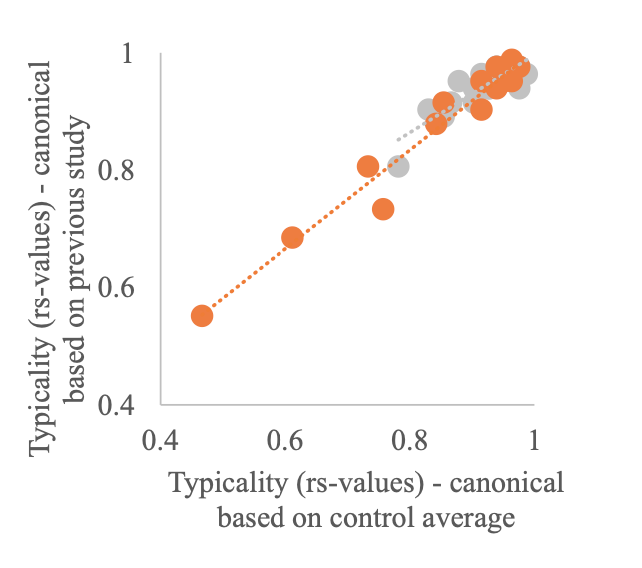
We then repeated all analysis using these newly calculated typicality scores. As expected, we found the same results as when using a canonical RDM based on the independent dataset (see below for details). This analysis has been added to the revised Appendix 1 and is referred to in the main manuscript.
Revised text Introduction:
“To investigate whether fine-grained hand somatotopy was preserved and could be activated in S1 following SCI, we assessed inter-finger representational distance patterns using representational similarity analysis (RSA). These inter-finger distance patterns are thought to be shaped by daily life experience such that fingers used more frequently together in daily life have lower representational distances (Ejaz et al., 2015). RSA-based inter-finger distance patterns have been shown to depict the invariant representational structure of fingers in S1 and M1 better than the size, shape, and exact location of the areas activated by finger movements (Ejaz et al., 2015). Over the past years RSA has therefore regularly been used to investigate somatotopy of finger representations both in healthy (e.g., Akselrod et al., 2017; Ariani et al., 2020; Ejaz et al., 2015; Gooijers et al., 2021; Kieliba et al., 2021; Kolasinski et al., 2016; Liu et al., 2021; Sanders et al., 2019) and patient populations (e.g., Dempsey- Jones et al., 2019; Ejaz et al., 2016; Kikkert et al., 2016; Wesselink et al., 2019). We closely followed procedures that have previously been used to map preserved and typical somatotopic finger selectivity and inter-finger representational distance patterns of amputees’ missing hands in S1 using volitional phantom finger movements (Kikkert et al., 2016; Wesselink et al., 2019).”
Revised text Results:
“This canonical RDM was based on 7T finger movement fMRI data in an independently acquired cohort of healthy controls (n = 8). The S1 hand ROI used to calculated this canonical RDM was defined similarly as in the current study (see Wesselink and Maimon- Mor, (2017b) for details). Note that results were unchanged when calculating typicality scores using a canonical RDM based on the averaged RDM of the age-, sex-, and handedness-matched control group tested in this study (see Appendix 1).”
Revised text Methods:
“While the traditional traveling wave approach is powerful to uncover the somatotopic finger arrangement, a fuller description of hand representation can be obtained by taking into account the entire fine-grained activity pattern of all fingers. RSA-based inter-finger overlap patterns have been shown to depict the invariant representational structure of fingers better than the size, shape, and exact location of the areas activated by finger movements (Ejaz et al., 2015). RSA-based measures are furthermore not prone to some of the problems of measurements of finger selectivity (e.g., dependence on map thresholds).”
“Third, we estimated the somatotopic typicality (or normality) of each participant’s RDM by calculating a Spearman correlation with a canonical RDM. We followed previously described procedures for calculating the typicality score (Dempsey-Jones et al., 2019; Ejaz et al., 2015; Kieliba et al., 2021; Wesselink et al., 2019). The canonical RDM was based on 7T finger movement fMRI data in an independently acquired cohort of healthy controls (n = 8). The S1 hand ROI used to calculated this canonical RDM was defined similarly as in the current study (see Wesselink and Maimon-Mor, (2017b) for details). Note that results were unchanged when calculating typicality scores using a canonical RDM based on the averaged RDM of the sex-, handedness-, and age matched control group tested in this study (see Appendix 1).”
Revised text Appendix 1:
“Typicality analysis using a canonical RDM based on the controls’ average RDM
To ensure that our typicality results did not change when using a canonical inter-finger RDM based on the age-, sex-, and handedness matched subjects tested in this study, we recalculated the typicality scores of all participants using the averaged inter-finger RDM of our control sample as the canonical RDM. We found a strong and highly significant correlation between the typicality scores calculated using the canonical inter-finger RDM from the independent dataset (reported in the main manuscript) and the typicality scores calculated using our controls’ average RDM. This was true for both the SCI patient (rs = 0.92, p < 0.001) and control groups (rs = 0.78, p < 0.001).
We then repeated all typicality analysis reported in the main manuscript. As expected, using the typicality scores calculated using our controls’ average RDM we found the same results as when using the canonical inter-finger RDM from the independent dataset: There was a significant difference in typicality between SCI patients, healthy controls, and congenital one-handers (H(2)=27.61, p < 0.001). We further found significantly higher typicality in controls compared to congenital one-handers (U=0, p < 0.001; BF10=76.11). Importantly, the typicality scores of the SCI patients were significantly higher than the congenital one-handers (U=2, p < 0.001; BF10=50.98), but not significantly different from the controls (U=94, p=0.24; BF10=0.55). Number of years since SCI significantly correlated with hand representation typicality (rs=-0.54, p=0.05) and patients with more retained GRASSP motor function of the tested upper limb had more typical hand representations in S1 (rs=0.58, p=0.03). There was no significant correlation between S1 hand representation typicality and GRASSP sensory function of the tested upper limb, spared midsagittal spinal tissue bridges at the lesion level, or cross-sectional spinal cord area (rs=0.40, p=0.15, rs=0.50, p=0.10, and rs=0.48, p=0.08, respectively). An exploratory stepwise linear regression analysis revealed that years since SCI significantly predicted hand representation typicality in S1 with R2=0.33 (F(1,10)=4.98, p=0.05). Motor function, sensory function, spared midsagittal spinal tissue bridges at the lesion level, and spinal cord area did not significantly add to the prediction (t=1.31, p=0.22, t=1.62, p=0.14, t=1.70, p=0.12, and t=1.09, p=0.30, respectively).”
- Methods & Results: The authors make a few unproven claims, such as saying "generally, the position, order of finger preference, and extent of the hand maps were qualitatively similar between patients and control". There are no data to support these claims.
As indicated in this sentence, this claim substantiated a qualitative inspection of the finger maps in Figure 2 and we indeed do not support this claim with quantitative analysis. We have therefore removed this sentence from the revised manuscript and instead say, as per the suggestion of reviewer 1, that overall, there were aspects of somatotopic finger selectivity in the SCI patients’ hand maps,
Revised text Results:
“Overall, we found aspects of somatotopic finger selectivity in the maps of SCI patients’ hands, in which neighbouring clusters showed selectivity for neighbouring fingers in contralateral S1, similar to those observed in eighteen age-, sex-, and handedness matched healthy controls (see Figure 2A&B). A characteristic hand map shows a gradient of finger preference, progressing from the thumb (red, laterally) to the little finger (pink, medially). Notably, a characteristic hand map was even found in a patient who suffered complete paralysis and sensory deprivation of the hands (Figure 2. patient map 1; patient S01). Despite most maps (Figure 2, except patient map 3) displaying aspects of characteristic finger selectivity, some finger representations were not visible in the thresholded patient and control maps.”
- Methods & Results: The authors argue that the map architecture is topographic as soon as the dissimilarity between two different fingers is above 0. First, what I am really wondering about is why the authors do not provide the exact dissimilarity values in the text but only give the stats for the difference to 0 (t-value, p-value, Bayes factor). Were the dissimilarity values perhaps very low? The values should be reported. Also, when this argument that maps are topographic as long as the value of two different fingers is above 0 should hold, then the authors have to show that the value for mapping the SAME finger is indeed 0. Otherwise, this argument is not convincing.
We would like to clarify that a representation is not per se topographic when the RSA dissimilarity is > 0. The dissimilarity value provided by RSA indicates the extent to which a pair of conditions is distinguished – it can be viewed as encapsulating the information content carried by the region (Kriegeskorte et al., 2008). Due to cross-validation across runs, the expected distance value would be zero (but can go below 0) if two conditions’ activity patterns are not statistically different from each other, and larger than zero if there is differentiation between the conditions (fingers’ activity patterns in the S1 hand area in our case; Kriegeskorte et al., 2008; Nili et al., 2014). The diagonal of the RDM reflect comparisons between the same fingers and therefore reflect distances between the exact same activity pattern in the same run and are thus 0 by definition (Kriegeskorte et al., 2008; Nili et al., 2014). This was also the case in our individual participant RDMs. Since this is not a meaningful value (a distance between 2 identical activity patterns will always be 0) we chose not to report this. We have clarified the meaning of the separability measure in the revised Methods section.
To investigate whether a representation is somatotopic, we have to take into account the full fine-grained inter-finger distance pattern. The full fine-grained inter-finger distance pattern is related to everyday use of our hand and has been shown to depict the invariant representational structure of fingers better than the size, shape, and exact location of the areas activated by finger movements (Ejaz et al., 2015). To determine whether a participant’s inter-finger distance pattern is somatotopic one should associate it to a canonical RDM – which is done in the typicality analysis (see also our response to comment 2.6).
What can be done to demonstrate the validity of an ROI, is to run RSA on a control ROI where one would not expect to find activity that is distinguishable between finger conditions. Rather than comparing your separability measure against 0, one can then compare the separability of your ROI that is expected to contain this information to that of your control ROI. We created a cerebral spinal fluid (CSF) ROI, repeated our RSA analysis in this ROI, and then compared the separability of the CSF and S1 hand area ROIs. As expected, there was a significant difference between separability (or representation strength) in the S1 hand area and CSF ROIs for both controls (W=171, p < 0.001; BF10=4059) and patients (W=105, p < 0.00; BF10=279). This analysis has been added to the revised manuscript.
Individual participant separability values (i.e., distances averaged across fingers) are visualised in Figure 3D. Following the reviewer’s suggestion, we have included individual participant inter-finger distance plots for both the controls and SCI patients as Figure 3- Figure supplement 2 and Figure 3- figure supplement 3, respectively. The inter-finger distances for each finger pair and subject can be extracted from this. We feel this is more readily readable and interpretable than a table containing the 10 inter-finger distance scores for all 32 participants. These values have instead been made available online, together with our other data, on https://osf.io/e8u95/.
Revised text Methods:
“If there is no information in the ROI that can statistically distinguish between the finger conditions, then due to cross-validation the expected distance measure would be 0. If there is differentiation between the finger conditions, the separability would be larger than 0 (Nili et al., 2014). Note that this does not directly indicate that this region contains topographic information, but rather that this ROI contains information that can distinguish between the finger conditions. To further ensure that our S1 hand ROI was activated distinctly for different fingers, we created a cerebral spinal fluid (CSF) ROI that would not contain finger specific information. We then repeated our RSA analysis in this ROI and statistically compared the separability of the CSF and S1 hand area ROIs.”
Revised text Results:
“We found that inter-finger separability in the S1 hand area was greater than 0 for patients (t(13) = 9.83, p < 0.001; BF10 = 6.77e +4) and controls (t(17) = 11.70, p < 0.001; BF10 = 6.92e +6), indicating that the S1 hand area in both groups contained information about individuated finger representations. Furthermore, for both controls (W = 171, p < 0.001; BF10 = 4059) and patients (W = 105, p < 0.001; BF10 = 279) there was significant greater separability (or representation strength) in the S1 hand area than in a control cerebral spinal fluid ROI that would not be expected to contain finger specific information. We did not find a significant group difference in inter-finger separability of the S1 hand area (t(30) = 1.52, p = 0.14; BF10 = 0.81), with the BF showing anecdotal evidence in favour of the null hypothesis.”
- Discussion. The authors argue that spared midsagittal spinal tissue bridges are not necessary because they were not predictive of hand representation typicality. First, the measure of typicality is questionable and should not be used to make general claims about the importance of structural differences. Second, given there were only n=14 patients included, one may question generally whether predictive modelling can be done with these data. This statement should therefore be removed.
We would like to clarify that, like the reviewer, we do not believe that spared midsagittal spinal tissue bridges are unimportant. Indeed, a large body of our own research focuses on the importance of spared spinal tissue bridges in recovery of sensorimotor function and pain (Huber et al., 2017; Pfyffer et al., 2021, 2019; Vallotton et al., 2019). We have added a clarification sentence regarding the importance of tissue bridges with regards to recovery of function. We agree with the reviewer that given our limited sample size, it is difficult to make conclusive claims based on non-significant predictive modelling and correlational results. In the revised manuscript we therefore focus this statement (i.e., that sensory and motor hand function and tissue bridges are not necessary to preserve hand somatotopy) on our finding that two patients without spared tissue bridges at the lesion level and with complete or near complete loss of sensory and motor hand function had a highly typical hand representation. We present our predictive modelling results as being in line with this notion and added a word of caution that it is challenging to draw definite conclusions from non-significant predictive modelling and correlation results in such a limited sample size.
With regards to the reviewer’s concern about the validity of the typicality measure – please see our detailed response to comment 2.6.
Revised text Discussion:
“Spared spinal cord tissue bridges can be found in most patients with a clinically incomplete injury, their width being predictive of electrophysiological information flow, recovery of sensorimotor function, and neuropathic pain (Huber et al., 2017; Pfyffer et al., 2021, 2019; Vallotton et al., 2019). However, in this study, spared midsagittal spinal tissue bridges at the lesion level and sensorimotor hand function did not seem necessary to maintain and activate a somatotopic hand representation in S1. We found a highly typical hand representation in two patients (S01 and S03) who did not have any spared spinal tissue bridges at the lesion level, a complete (S01) or near complete (S03) hand paralysis, and a complete (S01) or near complete loss (S03) of hand sensory function. Our predictive modelling results were in line with this notion and showed that these behavioural and structural spinal cord determinants were not predictive of hand representation typicality. Note however that our sample size was limited, and it is challenging to draw definite conclusions from non-significant predictive modelling results.”
- Discussion. The authors say that hand representation is "preserved" in SCI patients. Perhaps it is better to be precise and to say that they active during movement planning.
We thank the reviewer for their suggestion and revised the Discussion accordingly.
Revised text Discussion:
"In this study we investigated whether hand somatotopy is preserved and can be activated through attempted movements following tetraplegia."
"How may these representations be preserved over time and activated through attempted movements in the absence of peripheral information?"
"Together, our findings indicate that in the first years after a tetraplegia, the somatotopic S1 hand representation is preserved and can be activated through attempted movements even in the absence of retained sensory function, motor function, and spared spinal tissue bridges."
Reviewer #3:
The demonstration that cortex associated with an amputated limb can be activated by other body parts after amputation has been interpreted as evidence that the deafferented cortex "reorganizes" and assumes a new function. However, other studies suggest that the somatotopic organization of somatosensory cortex in amputees is relatively spared, even when probed long after amputation. One possibility is that the stability is due to residual peripheral input. In this study, Kikkert et al. examine the somatotopic organization of somatosensory cortex in patients whose spinal cord injury has led to tetraplegia. They find that the somatotopic organization of the hand representation of somatosensory cortex is relatively spared in these patients. Surprisingly, the amount of spared sensorimotor function is a poor predictor of the stability of the patients' hand somatotopy. Nonethless, the hand representation deteriorates over decades after the injury. These findings contribute to a developing story on how sensory representations are formed and maintained and provide a counterpoint to extreme interpretations of the "reorganization" hypothesis mentioned above. Furthermore, the stability of body maps in somatosensory cortex after spinal cord injury has implications for the development of brain-machine interfaces.
I have only minor comments:
1) Given the controversy in the field, the use of the phrase "take over the deprived territory" (line 45) is muddled. Perhaps a more nuanced exposition of this phenomenon is in order?
We agree a more nuanced expression would be more appropriate. We have changed this sentence accordingly in the revised manuscript.
Revised text Introduction:
“Seminal research in nonhuman primate models of SCI has shown that this leads to extensive cortical reorganisation, such that tactile stimulation of cortically adjacent body parts (e.g. of the face) activated the deprived brain territory (e.g. of the hand; Halder et al., 2018; Jain et al., 2008; Kambi et al., 2014).”
2) The statement that "results are mixed" regarding intracortical microstimulation of S1 is dubious. In only one case has the hand representation been mislocalized, out of many cases (several at CalTech, 3 at the University of Pittsburgh, one at Case Western, one at Hopkins/APL, and one at UChicago). Perhaps rephrase to "with one exception?"
We agree that this sentence may give a wrong outlook on the literature and have changed the text per the reviewer’s suggestion.
Revised text Introduction:
“Case studies using intracortical stimulation in the S1 hand area to elicit finger sensations in SCI patients hint at such preserved somatotopic representations (Fifer et al., 2020; Flesher et al., 2016), with one exception (Armenta Salas et al., 2018).”
3) The phrase "tetraplegic sinal cord injury" seems awkward.
Thank you for highlighting this to us. We have corrected these instances in our revised manuscript to “tetraplegia”.
4) The stability of the representation is attributed to efference copy from M1. While this is a fine speculation, somatosensory cortex is part of a circuit and is interconnected with many other brain areas, M1 being one. Perhaps the stability is maintained due to the position of somatosensory cortex within this circuit, and not solely by its relationship with M1? There seems to be an overemphasis of this hypothesis at the exclusion of others.
Thank you for this comment. We agree we overemphasized the efference copy theory. We have adjusted this and now provide a more balanced description of potential circuits and interconnections that could maintain somatotopic representations after tetraplegia.
Author Response:
Reviewer #1 (Public Review):
In this report, Shekhar et al, have profiled developing retinal ganglion cells from embryonic and postnatal mouse retina to explore the diversification of this class of neurons into specific subtypes. In mature retina, scRNAseq and other methods have defined approximately 45 different subtypes of RGCs, and the authors ask whether these arise from a common postmitotic precursor, or many ditinct subtypes of precursors. The overall message, is that subtype diversification arises as a "gradual, asynchronus fate restriction of postmitotic multipotential precursors. The authors find that over time, clusters of cells become "decoupled" as they split into subclusters. This process of fate decoupling is associated with changes in the expression of specific transcription factors. This allows them to both predict lineage relationships among RGC subtypes and the time during development when these specification events occur. Although this conclusion based almost entirely on a computational analysis of the relationships among cells sampled at discrete times, the evidence presented supports the overall conclusion. Future experimental validation of the proposed lineage relationships of RGC subtypes will be needed, but this report clearly outlines the overall pattern of diversification in this cell class.
We thank the reviewer for their thoughtful assessment of our study.
Reviewer #2 (Public Review):
The manuscript "Diversification of multipotential postmitotic mouse retinal ganglion cell precursors into discrete types" by Shekhar and colleagues represents an in-depth analysis of an additional transcriptomic datasets of retinal single-cells. It explores the progression of retinal ganglion cells diversity during development and describes some of aspects of fate acquisition in these postmitotic neurons. Altogether the findings provide another resource on which the neural development community will be able to generate new hypotheses in the field of retinal ganglion cell differentiation. A key point that is made by the authors regards the progression of the number of ganglion cell types in the mouse retina, i.e., how, and when neuronal "classes diversify into subclasses and types" (also p. 125). In particular, the authors would like to address whether postmitotic neurons follow either a predetermination or a stepwise progression (Fig. 2a). This is indeed a fascinating question, and the analysis, including the one based on the Waddington-OT method is conceptually interesting.
Comments and questions:
Is the transcriptomic diversity, based on highly variable genes (the number of which is not detailed in the study) a robust proxy to assess cell types? One could argue that early on predetermined cell types are specified by a small set of determinants, both at the proteomic and transcriptomic level, and that it takes several days or week to generate the cascade that allows the detection of transcriptional diversity at the level of >100 gene expression levels.
We had tested the dependence of our results on the number of highly variable genes (HVGs) used. This analysis, shown in Figure 2h, demonstrates that results are robust over the range tested – 1244-3003 total HVGs. Since the analysis in the paper employs 2800 HVGs (~800- 1500 at each stage), we are confident that we are in comfortable excess of the number at which we would need to worry. We have expanded the discussion to avoid confusion on this point. We also address the possibility that a small set of determinants are sufficient to define cell state in a transcriptomic study. This is a common argument, but we believe it is a tenuous one. We believe that the only way a small number of genes can truly define cell state is if they are expressed at very high levels. If these are expressed at high levels, they should be detected in our data and should drive the clustering. If they are expressed at extremely low levels, then given the nature of molecular fluctuations in cells, they cannot be expected to serve as a stable scaffold for differentiation. Indeed, a small set of determinants (usually transcription factors) may be necessary to specify a cell type. However, sufficiency of specification requires the expression of a usually much larger of number downstream regulators.
Since there are many RGC subsets (45) that share a great number of their gene expression, is it possible that a given RGC could transition from one subset to another between P5 and P56? Or even responding to a state linked to sustained activity? Was this possibility tested in the model?
We cannot address the possibility that cells swap types postnatally so that the cells comprising type X at P5 are not the same ones that comprise type X at P56. It does seem pretty unlikely, as the cell types are well-separated in transcriptional space (~250 DE genes on average). Regarding activity, we have made some initial tests by preventing visually evoked activity from birth to P56 in three different ways (dark-rearing and two mutant lines). We find no statistically significant effect on diversification. These results are currently being prepared for publication.
The authors state that early during development there is less diversity than later. This statement seems obvious but how much. Can this be due to differential differentiation stage? At E16 RGC are a mix of cells born from E11 to E16, with the latter barely located in the GCL. Does this tend to show a continuum that is may be probably lost when the analysis is performed on cells isolated a long time after they were born (postnatal stages)? Alternatively, would it be possible to compare RGC that have been label with birth dating methods?
Regarding the amount of diversification, we quantified this using the Rao diversity index (Figure 2h), which suggests an overall increase in 2-fold transcriptional diversity at P56 compared to the early stages. The continuum is likely because cells at early stage are close to the precursor stage and not very differentiated. Regarding combining RNA-seq with birthdating, although elegant methods now make this combination possible, it falls beyond the scope of this study.
Comparing data produced by different methods can be challenging. Here the authors compared transcriptomic diversity between embryonic dataset produced with 10X genomics (E13 to P0) and, on the other hand, postnatal P5 that were produced using a different drop-seq procedure). Is it possible to control that the differences observed are not due to the different methods?
It is correct that most of the P5 data was produced using Drop-seq, but that dataset also includes transcriptomes obtained by the 10X method. The relative frequency of RGC clusters and the average gene expression values obtained using either method was highly correlated (Reviewer Fig. 1). This is now pointed out in the “Methods.”
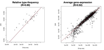
Reviewer Fig. 1. Comparison between the relative frequency of types (left) and the average gene expression levels (right) at P5 between 10X data (y-axis) and Drop-seq data (x-axis). R corresponds to the Pearson correlation coefficient. The axes are plotted in the logarithmic scale.
It might be important to control the conclusion that diversity is lower at E13 vs P5 when we see that thrice less cells (5900 vs 180000) were analyzed at early stage (BrdU, EdU, CFSE...)? A simple downsampling prior to the analysis may help.
Although we collected different numbers of cells at different ages, we noted in the text that they do not influence the number of clusters. Regarding P5 specifically, Rheaume et al. (who we now discuss) obtained very similar results to ours with only 6000 cells (3x lower).
Ipsilateral RGC: It is striking that the DEG between C-RGC and I-RGC reflect a strong bias with cells scored as" ipsi" are immature RGC while the other ("contra") are much more mature. This bias comes from the way ipsilateral RGC were "inferred" using non-specific markers. Can the author try again the analysis by identifying RGC using more robust markers? (eg. EphB1). Would it be possible to select I-RGC and C-RGC that share same level of differentiation? Previous studies already identified I-RGC signature using more specific set-up (Wang et al., 2016 from retrogradely labelled RGC; Lo Giudice et al., 2019 with I-RGC specific transgenic mouse).
We are not sure how the reviewer concludes that the putative I-RGCs are more immature than the putative C-RGCs. As discussed earlier, insofar as expression levels of pan-RGC markers are indicative of maturational stage, we found no evidence that clustering is driven by maturation gradients. Thus, we expect our putative I-RGCs and C-RGCs to not differ in differentiation state. Following the reviewer’s suggestion, we now include EphB1(Ephb1) in our I-RGC signature. The impact of replacing Igfbp5 with Ephb1 on the inferred proportion of I-RGCs within each terminal type was minimal (Reviewer Fig. 2). We would like to note that to assemble our IRGC/C-RGC signatures we relied on data presented Wang et al. (2016). Outside of wellestablished markers (e.g. Zic2, and Isl2), we chose the RNA-seq hits in Wang et al. that had been validated histologically in the same paper or that are correlated with Zic2 expression in our data. This nominated Igfbp5, Zic1, Fgf12, and Igf1.
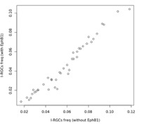
Reviewer Fig. 2. Comparison of inferred I-RGC frequency within each terminal type (points) using two I-RGC signature reported in the paper. For the y-axis we used Zic2 and EphB1.
It would be important to discuss how their findings differs from the others (including Rheaume et al., 2018). To make a strong point, I-RGC shall be isolated at a stage of final maturation (P5?) and using retrograde labelling, which is a robust method to ensure the ipsilateral identity of postnatal RGCs.
We cite Rheaume et al. in several places. In fact, there is good transcriptional correspondence between our dataset and theirs (Figure S1i), despite the differences in the number of cells profiled (~6000 vs ~18000) and technologies (10X vs. Drop-seq/10X). We now mention this is the text. Note also that we had compared our P56 data with Rheaume et al.’s, P5 data in an earlier publication (Tran et al., 2019) and observed a similar tight correspondence between clusters. Zic1 is expressed in I-RGCs (Wang et al., 2016) at early stages, and in our dataset its expression at E13 and E14 is similar to that of Zic2 (Supplementary Fig. 8); Postnatally, however, it marks W3B RGCs (Tran et al., 2019), many of which project contralaterally (Kim et al., J. Neurosci. 2010). Regarding retrograde labeling, as noted above, additional experiments would take a prohibitively long time (up to a year) to complete.
It is unclear how good Zic1 and Igf1 can be used as I-RGC marker. Can the author specify how specific to I-RGC they are? Have they been confirmed as marker using retrograde labelling experiments?
We have relied on previous work, primarily from the Mason lab, to choose I-RGC and C-RGC markers. Igf1 is a C-RGC marker that is expressed in a complementary fashion with Igfbp5, an I-RGC marker as noted in Wang et al, 2016. They also perform ISH to show that Igf1 is not expressed in the VT crescent, while Igfbp5 is (see Fig. 5 in Wang et al., 2016). Similarly, Zic1 is also cited in Wang et al. as an RNA-seq hit for I-RGCs. Although Zic1 was not validated using ISH, we found its expression pattern to be highly correlated with Zic2 at E13 (Supplementary Fig. 8c).
The enrichment procedure may deplete the RGC subpopulation that express low levels of Thy1 or L1CAM. A comparison on that point could be done with the other datasets analysed in the study.
We presume the reviewer is referring to the data of Lo Guidice and Clark/Blackshaw, which we show in comparison to ours in Figure S1. In both of those studies, all retinal cells were analyzed, whereas we enriched RGCs. As noted in the text, RGCs comprise a very small fraction of all retinal cells, so Lo Giudice and Clark/Blackshaw lacked the resolution to resolve RGC diversity at later time points. Indeed, there is no whole retina dataset available in which RGCs are numerous enough for comprehensive subtyping. Our approach to this issue was to collect RGCs with both Thy1 and L1 at E13, E14, E16 and P0, with the idea that the markers might have complementary strengths and weaknesses. In fact, at each age, all clusters are present in both collection types, although frequencies vary. This concordance supports the idea that neither marker excludes particular types. We now stress this point in results and in the Supplementary Fig. 2 legend.
In supplemental Fig. S1e: why are cells embedded from "Clark" datasets only clusters on the right side of the UMAP while the others are more evenly distributed?
Actually, both the Clark et al. and Lo Giudice et al. datasets are predominantly clustered on the right side of the UMAP. This reflects the methodological difference noted above: they profiled the whole retina, whereas we isolated RGCs. Thus, their datasets contain a much higher abundance of RPCs and non-neurogenic precursors compared to ours. The right clusters represent RPCs due to their expression of Fgf15 and other markers, while the left clusters represent RGCs based on their expression of Nefl. Indeed, a main reason for including these plots was to illustrate the relative abundance of RGCs in our data (also see Supplementary Fig. S1h).
What could explain that CD90 and L1CAM population are intermingled at E14, distinct at E16, and then more mixed at P0?
We believe the reviewer is referring to Supplementary Figs. S2a-c. Given the temporal expression level changes in Thy1 and L1cam (Supplementary Fig. S1c) in RGCs, a likely possibility is that they enrich RGC precursor subsets at different relative frequencies. We now note this in the Supplementary Fig. 2 legend.
On Fig. 6: the E13 RGC seems to be segregated in early born RGC expressing Eomes and later born expressing neurod2. Thus, fare coupling with P5 seems to suggest that Eomes population at P5 may have been generated first, and Neurod2 generated later. Is that possible?
That the Eomes RGCs are specified before Neurod2 RGCs is one of our conclusions from the fate decoupling analysis (Figures 6f-h). Whether this is because the former arise from early born cells and the latter arise from later born cells is not clear. There is disagreement in the literature on whether ipRGCs are born at a different time than other RGCs, so we prefer not to make a comment.
Methods: The Methods section is extensive, and yet it is presented in a rather complex manner so that it is difficult to understand for a broad audience. It would be valuable if the authors could simplify or better explain some parts (the WOT section in particular).
We believe that the sections on animals, molecular biology and histology are quite straightforward, but agree that the sections describing the computational analysis are hard going. We have modified them in several places as requested. As regards better explanation of the WOT, we now precede that section with an “overview” as a way of making it easier to follow. (We had already included an overview of the clustering procedures.) We have also provided further detail on some of the reviewer’s subsequent questions on this section, including the use of HVGs, the Classifier, and the strategy for inferring I-RGCs (see below). Perhaps most important, we have worked to make the “Results” and “Discussion” sections accessible to a broad audience.
*Highly variable genes (HVG) used for clustering and dimensionality reduction: how many of them and what are they? Are they the same used for each stage?
Since clustering was performed at each stage independently, we determined HVGs at each stage separately using a statistical method introduced in one of our previous studies (Pandey et al., Current Biology, 2018). The total number of HVGs at each stage were as follows: E13: N=1094 E14: N=834 E16: N=822 P0: N=881 P5: N=1105 P56: N=1510
We note that these are not necessarily the same at each stage due to the temporal variation in gene expression. Together these correspond to 2854 unique genes (union of all HVGs). The WOT analysis was done using this full set.
*In the methods p9: "The common features G = GR ∩ GT are used to train a third classifier ClassR on the reference atlas AR. This ensures that inferred transcriptomic correspondences are based on "core" gene expression programs that underlie cell type identity rather than maturation-associated genes." Could the authors explain the relevance of using a third model and, more importantly, is there any genes that eliminated through the procedure that could be important to drive the diversification process? If so, would it be possible to estimate their number and the relative impact?
The rationale for this was as follows. Our goal is to map cells from one time point to a type at another time point. The naïve way to do this would be to use a classifier trained entirely at either of the time point. However, the features of such a classifier is likely to contain genes that are not expressed at the earlier time point, and likely to generate spurious mappings (since the set of cluster specific genes are not identical). Therefore, we sought to train a classifier that is trained using genes that are part of conserved transcriptional signatures at both time points, which corresponds to the third model.
When this filtering was not performed, the temporal correspondences in the supervised classification model were less specific than those reported. In particular, ARI values dropped by about 15% on average. The simple reason for this is that a cluster specific gene at E13 (for e.g.) may no longer be expressed at E14, and vice-versa. Thus, by restricting the features to a common set of cluster specific genes, we obtained the “best possible” transcriptomic correspondences between clusters at consecutive time points. We note that the correspondences obtained in this way (Figure 3) were recovered through WOT when the results of the latter were collapsed at the cluster level (Supplementary Fig. 5).
*Methods page 15: Inference of ipsilaterally-projecting RGC types. Wouldn't it be more valuable to consider more markers to distinguish RGC precursors?
As indicated before, we used I-RGC genes and C-RGC genes reported in Wang et al., 2016 (Table 2), in addition to the well-known markers Zic2 and Isl2. Here, we prioritized genes that had been histologically validated (Figs. 4 and 5), which were expressed in our data (Sema3e and Tbx20 were not considered as these undetectable at E13 in our data). Following the reviewer’s earlier suggestion, we also noted that including Ephb1 in our signature minimally impacts the results.
Discussion: *Is there somewhat a plasticity that allow the RGC subgroups to switch over time? (IF we were to record the transcriptome of the same cell over time, will one observe that the cell belong to another cluster / subgroup?
One can only speculate. Other than long-term in vivo imaging combined with vital type-specific markers we know of no way to experimentally address the possibility that cells swap types postnatally so that the cells comprising type x at P5 are not the same ones that comprise type x at P56. It does seem pretty unlikely though.
*While the data appears technically rigorous, and the number of cells sequenced very high, the results seem redundant with several prior studies and the discrepancies are not sufficiently discussed.
We are confused by this point, since the reviewer does not cite the papers to which s/he refers. To our knowledge there is no study at present that has described RGC diversification, so it is not clear what would be discrepant.
Author Response
Reviewer #1 (Public Review):
It is well established that valuation and value-based decision-making is context-dependent. This manuscript presents the results of six behavioral experiments specifically designed to disentangle two prominent functional forms of value normalization during reward learning: divisive normalization and range normalization. The behavioral and modeling results are clear and convincing, showing that key features of choice behavior in the current setting are incompatible with divisive normalization but are well predicted by a non-linear transformation of range-normalized values.
Overall, this is an excellent study with important implications for reinforcement learning and decision-making research. The manuscript could be strengthened by examining individual variability in value normalization, as outlined below.
We thank the Reviewer for the positive appreciation of our work and for the very relevant suggestions. Please find our point-by-point answer below.
There is a lot of individual variation in the choice data that may potentially be explained by individual differences in normalization strategies. It would be important to examine whether there are any subgroups of subjects whose behavior is better explained by a divisive vs. range normalization process. Alternatively, it may be possible to compute an index that captures how much a given subject displays behavior compatible with divisive vs. range normalization. Seeing the distribution of such an index could provide insights into individual differences in normalization strategies.
Thank you for pointing this out, it is indeed true that there is some variability. To address this, and in line with the Reviewer’s suggestion, we extracted model attributions per participant on the individual out-of-sample log-likelihood, using the VBA_toolbox in Matlab (Daunizeau et al., 2014). In experiment 1 (presented in the main text), we found that the RANGE model accounted for 79% of the participants, while the DIVISIVE model accounted for 12%. The relative difference was even higher when including the RANGEω model in the model space: the RANGE and RANGEω models account for a total of 85% of the participants, while the DIVISIVE model accounted only for 5%.
In experiment 2 (presented in the supplementary materials), the results were comparable (see Figure 3-figure supplement 3: 73% vs 10%, 83% vs 2%).
To provide further insights into the behavioral signatures behind inter-individual differences, we plotted the transfer choice rates for each group of participants (best explained by the RANGE, DIVISIVE, or UNBIASED models), and the results are similar to our model predictions from Figure 1C:
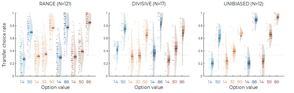
Author Response Image 1. Behavioral data in the transfer phase, split over participants best explained by the RANGE (left), DIVISIVE (middle) or UNBIASED (right) model in experiment 1 (A) and experiment 2 (B) (versions a, b and c were pooled together).
To keep things concise, we did not include this last figure in the revised manuscript, but it will be available for the interested readers in the Rebuttal letter.
One possibility currently not considered by the authors is that both forms of value normalization are at work at the same time. It would be interesting to see the results from a hybrid model. R1.2 Thank you for the suggestion, we fitted and simulated a hybrid model as a weighted sum between both forms of normalization:
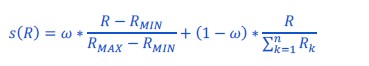
First, the HYBRID model quantitatively wins over the DIVISIVE model (oosLLHYB vs oosLLDIV : t(149)=10.19, p<.0001, d=0.41) but not over the RANGE model, which produced a marginally higher log-likelihood (oosLLHYB vs oosLLRAN : t(149)=-1.82, p=.07, d=-0.008). Second, model simulations also suggest that the model would predict a very similar (if not worse) behavior compared to the RANGE model (see figure below). This is supported by the distribution of the weight parameter over our participants: it appears that, consistently with the model attributions presented above, most participants are best explained by a range-normalization rule (weight > 0.5, 87% of the participants, see figure below). Together, these results favor the RANGE model over the DIVISIVE model in our task.
Out of curiosity, we also implemented a hybrid model as a weighted sum between absolute (UNBIASED model) and relative (RANGE model) valuations:
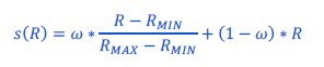
Model fitting, simulations and comparisons slightly favored this hybrid model over the UNBIASED model (oosLLHYB vs oosLLUNB: t(149)=2.63, p=.0094, d=0.15), but also drastically favored the range normalization account (oosLLHYB vs oosLLRAN : t(149)=-3.80, p=.00021, d=-0.40, see Author Response Image 2).
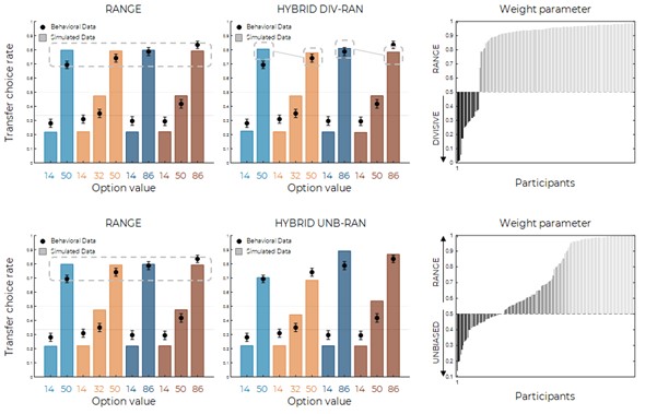
Author Response Image 2. Model simulations in the transfer phase for the RANGE model (left) and the HYBRID model (middle) defined as a weighted sum between divisive and range forms of normalization (top) and between unbiased (no normalization) and range normalization (bottom). The HYBRID model features an additional weight parameter, whose distribution favors the range normalization rule (right).
To keep things concise, we did not include this last figure in the revised manuscript, but it will be available for the interested readers in the Rebuttal letter.
Reviewer #2 (Public Review):
This paper studies how relative values are encoded in a learning task, and how they are subsequently used to make a decision. This is a topic that integrates multiple disciplines (psych, neuro, economics) and has generated significant interest. The experimental setting is based on previous work from this research team that has advanced the field's understanding of value coding in learning tasks. These experiments are well-designed to distinguish some predictions of different accounts for value encoding. However there is an additional treatment that would provide an additional (strong) test of these theories: RN would make an equivalent set of predictions if the range were equivalently adjusted downward instead (for example by adding a "68" option to "50" and "86", and then comparing to WB and WT). The predictions of DN would differ however because adding a low-value alternative to the normalization would not change it much. Would the behaviour of subjects be symmetric for equivalent ranges, as RN predicts? If so this would be a compelling result, because symmetry is a very strong theoretical assumption in this setting.
We thank the Reviewer for the overall positive appraisal concerning our work, but also for the stimulating and constructive remarks that we have addressed below. At this stage, we just wanted to mention that we also agree with the Reviewer concerning the fact that a design where we add "68" option to "50" and "86" would represent also an important test of our hypotheses. This is why we had, in fact, run this experiment. Unfortunately, their results were somehow buried in the Supplementary Materials of our original submission and not correctly highlighted in the main text. We modified the manuscript in order to make them more visible:
Behavioral results in three experiments (N=50 each) featuring a slightly different design, where we added a mid value option (NT68) between NT50 and NT87 converge to the same broad conclusion: the behavioral pattern in the transfer phase is largely incompatible with that predicted by outcome divisive normalization during the learning phase (Figure 2-figure supplement 2).
Reviewer #3 (Public Review):
Bavard & Palminteri extend their research program by devising a task that enables them to disassociate two types of normalisation: range normalisation (by which outcomes are normalised by the min and max of the options) and divisive normalisation (in which outcomes are normalised by the average of the options in ones context). By providing 4 different training contexts in which the range of outcomes and number of options vary, they successfully show using 'ex ante' simulations that different learning approaches during training (unbiased, divisive, range) should lead to different patterns of choice in a subsequent probe phase during which all options from the training are paired with one another generating novel choice pairings. These patterns are somewhat subtle but are elegantly unpacked. They then fit participants' training choices to different learning models and test how well these models predict probe phase choices. They find evidence - both in terms of quantitive (i.e. comparing out-of-sample log-likelihood scores) and qualitative (comparing the pattern of choices observed to the pattern that would be observed under each mode) fit - for the range model. This fit is further improved by adding a power parameter which suggests that alongside being relativised via range normalisation, outcomes were also transformed non-linearly.
I thought this approach to address their research question was really successful and the methods and results were strong, credible, and robust (owing to the number of experiments conducted, the design used and combination of approaches used). I do not think the paper has any major weaknesses. The paper is very clear and well-written which aids interpretability.
This is an important topic for understanding, predicting, and improving behaviour in a range of domains potentially. The findings will be of interest to researchers in interdisciplinary fields such as neuroeconomics and behavioural economics as well as reinforcement learning and cognitive psychology.
We thank Prof. Garrett for his positive evaluation and supportive attitude.
Author Response
Reviewer #1 (Public Review):
In this paper, Fernandes et al. take advantage of synthetic constructs to test how Bicoid (Bcd) activates its downstream target Hunchback (Hb). They explore synthetic constructs containing only Bcd, Bcd and Hb, and Bcd and Zelda binding sites. They use these to develop theoretical models for how Bcd drives Hb in the early embryo. They show that Hb sites alone are insufficient to drive further Hb expression.
The paper's first half focuses on how well the synthetic constructs replicate the in vivo expression of hb. This approach is generally convincing, and the results are interesting. Consistent with previous work, they show that Bcd alone is sufficient to drive an expression profile that is similar to wild‐type, but the addition of Hb and Zelda are needed to generate precise and rapid formation of the boundaries. The experimental results are supported by modelling. The model does a nice job of encapsulating the key conclusions and clearly adds value to the analysis.
In the second part of the paper, the authors use their synthetic approach to look at how the Hb boundary alters depending on Bcd dosage. This part asks whether the observed Bcd gradient is the same as the activity gradient of Bcd (i.e. the "active" part of Bcd is not a priori the same as the protein gradient). This is a very interesting problem and good the authors have tried to tackle this. However, the strength of their conclusions needs to be substantially tempered as they rely on an overestimation of the Bcd gradient decay length.
Comments:
‐ My major concern regards the conclusions for the final section on the activity gradient. In the Introduction it is stated: "[the Bcd gradient has] an exponential AP gradient with a decay length of L ~ 20% egg‐length (EL)". While this was the initial estimate (Houchmandzadeh et al., Nature 2002), later measurements by the Gregor lab (see Supplementary Material of Liu et al., PNAS 2013) found that "The mean length constant was reduced to 16.5 ± 0.7%EL after corrections for EGFP maturation". The original measurements by Houchmandzadeh et al. had issues with background control, that also led to the longer measured decay length. In later work, Durrieu et al., Mol Sys Biol 2018, found a similar scale for the decay length to Liu et al. Looking at Figure 5, a value of 16.5%EL for the decay length is fully consistent with the activity and protein gradients for Bcd being similar. In short, the strength of the conclusions clearly does not match the known gradient and should be substantially toned down.
The reviewer is right: several studies aiming to quantitatively measure the Bicoid protein gradient ended‐up with quite different decay lengths.
A summary of the various decay lengths measured, and the method used for these measurements is given below:
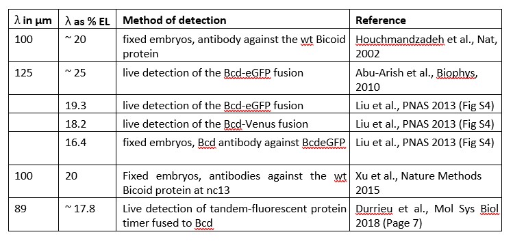
As indicated, these measurements are quite variable among the different studies and the differences can potentially be attributed to different methods of detection (antibody staining on fixed samples vs fluorescent measurements on live sample) or to the type of protein detected (endogenous Bicoid vs fluorescently tagged).
We agree with the reviewer that given these discrepancies, the exact value of the Bcd protein gradient decay length is not known and that we only have measurements that put it in between 16 and 25 % EL (see the Table above). Therefore, we agree that we should tone down the difference between the protein vs activity gradient and focus on the measurements of the effective activity gradient decay length allowed by our synthetic reporters. This allows us to revisit the measurement of the Hill coefficient of the transcription step‐like response, which is based on the decay‐length for the Bcd protein gradient, and assumed in previous published work to be of 20% EL (Gregor et al., Cell, 2007a; Estrada et al., 2016; Tran et al., PLoS CB, 2018). Importantly, the new Hill coefficient allows us to set the Bcd system within the limits of an equilibrium model.
As mentioned by the reviewer, it is possible that the decay length of the protein gradient measured using antibody staining (Houchmandzadeh et al,, Nature, 2002) was not correct due to background controls. Such measurements were also performed in Xu et al. (2015) which agree with the original measurements (Houchmandzadeh et al., Nature 2002). As indicated in the table above, all the other measurements of the Bcd protein gradient decay length were done using fluorescently tagged Bcd proteins and we cannot exclude the possibility the wt vs tagged protein might have different decay lengths due to potentially different diffusion coefficients or half‐lives. Before drawing any conclusion on the exact value of the endogenous Bcd protein gradient decay length, it is essential to measure it again in conditions that correct for the background issues for immuno‐staining as it was done in Liu et al., PNAS, 2013 for the Bcd‐eGFP protein. In this study, the authors only measured the decay length of the Bcd fusion protein using immuno‐staining for the Bcd protein. Unfortunately, in this study, the authors did not measure again the decay length of the endogenous Bcd protein gradient using immuno‐staining and the same procedure for background control. Therefore, they do not firmly exclude the possibility that the endogenous vs tagged Bcd proteins might have different decay length.
We thank the reviewer for his comment which helped us to clarify the message. In addition, as there is clearly an issue for the measurements of the Bcd protein gradient, we added a section in the SI (Section E) and a Table (Table S4) describing the various decay length measured for the Bcd or the Bcd‐fluorescently tagged protein gradients from previous studies. In the discussion, together with the possibility that there might be a protein vs activity gradient (as we originally proposed and believe is still a valid possibility), we also discuss the alternative possibility proposed by the reviewer which is that the protein vs activity gradients have the same decay lengths but that the decay length of the Bcd protein gradient was potentially not correctly evaluated.
‐ All of the experiments are performed in a background with the hb gene present. Does this impact on the readout, as the synthetic lines are essentially competing with the wild‐type genes? What controls were done to account for this?
We agree with the reviewer that this concern might be particularly relevant at the hb boundary where a nucleus has been shown to only contain ~ 700 Bicoid molecules (Gregor et al., Cell, 2007b). However, ~1000 Bicoid binding regions have been identified by ChIP seq experiments in nc14 embryos (Hannon et al., Elife, 2017) and given that several Bcd binding sites are generally clustered together in a Bcd region, the number of Bcd binding sites in the fly genome is likely larger than 1000. It is much greater than the number of Bicoid binding sites in our synthetic reporters. Therefore, we think that it is unlikely that adding the synthetic reporters (which in the case of B12 only represents at most 1/100 of the Bcd binding sites in the genome) will severely alter the competition for Bcd binding between the other Bcd binding sites in the genome. Additionally, the insertion of a BAC spanning the endogenous hb locus with all its Bcd‐dependent enhancers did not affect (as far as we can tell) the regulation of the wildtype gene (Lucas, Tran et al., 2018).
We have added a sentence concerning this point in the main text (lines 108 to 111).
‐ Further, the activity of the synthetic reporters depends on the location of insertion. Erceg et al. PLoS Genetics 2014 showed that the same synthetic enhancer can have different readout depending on its genomic location. I'm aware that the authors use a landing site that appears to replicate similar hb kinetics, but did they try random insertion or other landing site? In short, how robust are their results to the specific local genome site? This should have been tested, especially given the boldly written conclusions from the work.
This concern of the reviewer has been tested and is addressed Fig S1 where we compare two random insertions of the hb‐P2 transgene (on chromosome II and III; Lucas, Tran et al., 2018) and the insertion at the VK33 landing site that was used for the whole study. As shown Fig. S1, the dynamics of transcription (kymographs) are very similar. In the main text, the reference Fig. S1 is found in the Materials and Methods section (bottom of the 1st paragraph concerning the Drosophila stocks, lines 518).
‐ Related to the above, it's also not obvious that readout is linear ‐ i.e. as more binding sites are added, there could be cooperativity between binding domains. This may have been accounted for in the model but it is not clear to me how.
The reviewer is totally correct. It is clear from our data that readout is not linear: comparing (increase of 1.5 X in the number of BS) B6 with B9 leads to a 4.5 X greater activation rate and this argues against independent activation of transcription by individual bound Bcd TF. There is almost no impact of adding 3 more sites when comparing B9 to B12 (even though it corresponds to an increase of 1.33 X in the number of BS). This issue has been rephrased in the main text (lines 200 to 203) and further developed for the modeling aspects in the SI section C and Figure S3. It is also discussed in the second paragraph of the discussion (lines 380 to 383).
‐ It would be good in the Introduction/Discussion to give a broader perspective on the advantages and disadvantages of the synthetic approach to study gene regulation. The intro only discusses Tran et al. Yet, there is a strong history of using this approach, which has also helped to reveal some of the approaches shortcoming. E.g. Gertz et al. Nature 2009 and Sharon et al. Nature Biotechnology 2012. Again, I may have missed, but from my reading I cannot see any critical analysis of the pros/cons of the synthetic approach in development. This is necessary to give readers a clearer context.
One sentence was added in the introduction concerning this point (lines 79 to 82).
A short review concerning the synthetic approach in development has also been added at the beginning of the discussion (lines 347 to 359).
Reviewer #2 (Public Review):
It is known that Bicoid increases in concentration across the syncytial division cycles, the gradient length scale for Bicoid does not change, and hunchback also increases in concentration during the syncytial cycles but the sharp boundary of the hunchback gradient is constantly seen despite the change in concentration of Bicoid. This manuscript shows that by increasing the Bicoid concentration or by adding Zelda binding sites, the expression of hunchback can be recapitulated to that of a previously studied promoter for hunchback.
I have the following comments to understand the implications of the study in the context of increasing concentrations of Bicoid during the syncytial division cycles:
‐ Bicoid itself is also increasing over the syncytial division cycles, how does this change in concentration of Bicoid affect the activation of the hunchback promoter given the cooperative binding of Bicoid and Bicoid and Zelda as documented by the study?
We thank the reviewer for this remark about the dynamics of the Bcd gradient, which we may have taken for granted. A seminal work on the dynamics of the Bcd gradient using fluorescent‐tagged Bcd (Gregor et al, Cell, 2007a) has shown that the gradient of Bcd nuclear concentration (this nuclear concentration is the one that matter for transcription) remains stable over nuclear cycles, despite a global increase of Bcd amount in the embryo. This can be explained by the fact that Bcd molecules are imported in the nuclei and that the number of nuclei double at every cycle, such that both processes compensate each other. Thus, we assumed that the gradient of Bcd nuclear concentration was stable over nc11 to nc13.
We have clarified this assumption in the model section in the manuscript (lines 165‐168).
Supporting our assumption, when looking at the transcription dynamics regulated by Bcd, in Lucas et al, PLoS Gen, 2018, we observed very reproducible expression pattern dynamics of the hb‐P2 reporter at each cycle nc11 to nc13. Such reproducibility in the pattern dynamics were also observed in this current work for hb‐P2, B6, B9, B12 and H6B6 reporters (Fig. S6A). Also, in Lucas et al, PLoS Gen, 2018, the shift in the established boundary positions of hb‐P2 reporter between nc11 to nc13 is ~2%EL (approximately a nucleus length ~10μm) and it is thus marginal.
In addition, as mentioned in the text (lines 105 to 107), we only focused our analysis on nc13 data which are statistically stronger given the higher number of nuclei analyzed. Thus, any change of Bcd nuclear concentration that would happen over nuclear cycles will not matter.
Concerning Zelda: Zelda’s transcriptional activity when measured on a reporter with only 6 Zld binding sites changes drastically over the nuclear cycles, with strong activity at nc11 and much weaker activity at nc13 (Fig S4A). This indicates that the changes in expression pattern dynamics of Z2B6 from nc11 to nc13 are caused predominantly by decreasing Zelda activity: the effect of Zld on the Z2B6 promoter is very strong during nc11 and nc12. It is also very strong at the beginning of nc13 (even though the Z6 reporter is almost silent) and became a bit weaker in the second part of nc13 (Fig S4B‐D).
‐ Does the change in concentration of Bicoid across the nuclear cycles shift the gradient similar to the change in numbers of Bicoid binding sites?
In both Lucas et al, PLoS Gen, 2018 and in this work (Fig. 1, Fig. 3 and Fig. S6A), we found that the positions of the expression boundary are very reproducible and stable in time for hb‐P2, B6, B9, B12, H6B6 during the interphase of nc12 to 13. For hb‐P2, the averaged shift of the established boundary position in nc11, 12 and 13 is within 2 %EL. This averaged shift between the cycles is of similar magnitude to the difference caused by embryo‐to‐embryo variability within nc13 (~2 %EL) (Gregor et al, Cell, 2007b, Lucas et al, PloS Gen, 2018). This shift is much smaller than the difference between the expression boundary positions of B6 and B9 (~ 8 % EL) and between B6 and Z2B6 (~17.5 %EL) in nc13.
For these reasons, we conclude that the difference between the expression patterns of B6, B9 and Z2B6 are caused predominantly by changing the TF binding site configurations of the reporters, rather than variability in the Bcd gradient.
The assumption of gradient stability has been clarified in the previous answer and in the manuscript (lines 165‐168).
‐ The intensity is a little higher for B9 and B12 at the anterior in 2B? Is this statistically different? is this likely to change the amount of Bicoid expression at the locus and lead to more robust activation?
We performed statistical tests to distinguish the spot intensities at the anterior pole for every pair of reporters in Fig. 2B (hb‐P2, B6, B9 and B12). All p‐values from pair‐wise KS tests are greater than 0.067, suggesting that the spot intensities at the anterior pole are not distinguishable between these reporters.
We have clarified this in the manuscript (line 157).
‐Are the fraction of active loci not changing across the syncytial cycles when the concentration of Bicoid also changes and consistent with the synthetic promoters?
To measure the reproducibility of the expression pattern dynamics in different nuclear cycles, we compared the boundary position of the fraction of active loci pattern as a function of time for all hbP2 and synthetic reporters (Fig. S6A). In this figure panel, for all reporters except Z2B6, the curves in nc12 and nc13 largely overlap, suggesting high reproducibility in the pattern dynamics between cycles and consequently low sensitivity to the subtle variation in the Bcd nuclear concentration gradient between the cycles.
For Z2B6, we attributed the difference in pattern dynamics between nc12 and nc13 to the changes in Zelda activity, as validated independently with a synthetic reporter with only 6 Zld binding sites (Fig. S4A).
‐How do the numbers of Hb BS change the expression of Hb? H6B6 has 6 Hb BS whereas the Hb‐P2 has 1? Are more controls needed to compare these 2 contexts?
As our goal was to determine to which mechanistic step of our model each TF (Bcd, Hb, Zld) contributed, we added BS numbers that are much higher than in the hb‐P2 promoter. The added number of Hb BS remains very low when compared to total number of Hb binding sites in the entire genome (Karplan et al, PLOS Gen, 2011), therefore, it is very unlikely to affect the endogenous expression of Hb protein.
We clarified this in the manuscript (lines 211 to 212).
Does Zelda concentration change across the syncytial division cycles? How does the change in concentration in the natural context affect the promoter activation of Hb?
Zelda concentration is stable over the nuclear cycles, as observed with the fluorescently‐tagged Zld protein (Dufourt et al., Nat Com, 2018). However, Zelda’s transcriptional activity when measured on a reporter with only 6 Zld binding sites changes drastically over the nuclear cycles, with strong activity at nc11 and much weaker activity at nc13 (Fig S4A, this work).
The impact of this change in Zld activity can be observed with the Z2B6 promoter, with the expression boundary moving from the posterior region toward the anterior region over the nuclear cycles (Fig. S4B‐D). However, we don’t detect any changes in the expression pattern dynamics of hb‐P2 over the nuclear cycles (Fig. S6A and in Lucas et al., PLoS Gen, 2018).
We have clarified this in lines 250‐251 of the main manuscript.
‐Changing the dose of Bicoid shifts the boundary of hunchback expression. It would be nice to model or test this in the context of varing doses of zelda or even reason this with respect to varying doses of zelda across the syncytial division cycles.
We thank the reviewer for this insight. Concerning Zelda, we did not perform any experiment reducing the amount of Zelda in the embryo. However, in a previous study (Lucas et al., PLoS Genetics, 2018), we observed that the boundary of hb was shifted towards the anterior when decreasing the amount of Zelda consistent to the fact that the dose of Zelda is critical to set the boundary position and the threshold of Bcd concentration required for activation. However, as Zelda is distributed homogeneously along the AP axis, it cannot bring per se positional information to the system.
Reviewer #3 (Public Review):
I think the framing could be improved to better reflect the contribution of the work. From the abstract, for example, it's unclear to me what the authors think is the most meaningful conclusion. Is it the observations about the finer details of TF regulation (bursting dynamics), the fact that Bcd is probably the sole source of "positional information" for hb‐p2, that Bcd exists in active/inactive form, or the fact that an equilibrium model probably suffices to explain what we observe? The first sentence itself seems to suggest this paper will discuss "dynamic positional information", in which case it's somewhat misleading to say this kind of work is "largely unexplored"; Johannes Jaeger in particular has been a strong proponent of this view since at least 2004. On that note some particularly relevant recent papers in the Drosophila early embryo include:
1) Jaeger and Verd (2020) Curr Topics Dev Biol
2) Verd et al. (2017) PLoS Comp Biol
3) Huang, Amourda, et al. and Saunders (2017) eLife
4) Yang, Zhu, et al. (2020) eLife [see also the second half of Perkins (2021) PLoS Comp Biol for further discussion of that model]
‐Some reviews from James Briscoe also discuss this perspective.
We agree with the reviewer that the phrasing of the abstract was not clear enough to emphasize the contribution of the work and we are also sorry if it suggested that the dynamic positional information is largely unexplored because this was not at all our intention.
We rephrased the abstract aiming to better highlight the most meaningful conclusions.
‐I would also recommend modifying the title to reflect the biology found in the new results.
We modified the title to better reflect the new results:<br /> “Synthetic reconstruction of the hunchback promoter specifies the role of Bicoid, Zelda and Hunchback in the dynamics of its transcription”
‐A major point that the authors should address is the design of the synthetic constructs. From table S1, the sites are often very closely linked (4‐7 base pairs). From the footprint of these proteins, we know they can cover DNA across this size (see, https://pubmed.ncbi.nlm.nih.gov/8620846/). As such, there may be direct competition/steric hindrance (see https://pubmed.ncbi.nlm.nih.gov/28052257/). What impact does this have on their interpretations? Note also that the native enhancer has spaced sites with variable identities.
We completely agree with the reviewer comment in the sense that we named our reporters according to the number (N) of Bcd binding sites sequences that they contain, even though we cannot prove definitively that they can effectively be bound simultaneously by N Bcd molecules. It is thus possible that B9 is not a B9 but an effective B6 (i.e. B9 can only be bound simultaneously by 6 molecules) if, for instance, the binding of a Bcd molecule to one site would prevent by the binding of another Bcd molecule to a nearby site (as proposed by the reviewer in the case of direct competition or steric hindrance).
Even though we cannot exclude this possibility, we think that our use of B6, B9, B12, in reference to the 6 Bcd BS of hb‐P2 promoter, is relevant for several reasons : i) some of the Bcd BS in the hb‐P2 promoter are also very close from each other (see Table S1); ii) the design of the synthetic construct was made by multimerizing a series of 3 strong Bcd binding sites with a similar spacing as found for the closest sites in the hb‐P2 promoter (as shown in Figure 1A and Table S1); iii) the binding of the Bicoid protein has been shown in foot printing experiments in vitro to be more efficient on sites of the hb‐P2 promoter that are close from each other, and this has even been interpreted as binding cooperativity (Ma et al., 1996); iv) even though these experiments were not performed with full‐length proteins, two molecules of the paired homeodomain (from the same family of DNA binding domain as Bcd) are able to simultaneously bind to two binding sites separated by only 2 base pairs. This binding to very close sites is even cooperative while when the two sites are distant by 5 base pairs or more, the simultaneous binding to the two sites occurs without cooperativity (Wilson et al., 1993).
Conversely, as it is very difficult to demonstrate that 9 Bcd molecules can effectively bind to our B9 promoter, it is very difficult to know exactly how many binding sites for Bcd the hb‐P2 contains, and a large debate concerning not only the number but also the identity of the Bcd sites in the hb promoter is still ongoing (Park et al., 2019; Ling et al., 2019).
As we cannot exclude the possibility that B9 is an effective B6, it remains possible that B9 and hb‐P2 (which is supposed to only contains 6 sites) have the same number of effective Bcd binding site and this could explain why the two reporters have very similar transcription dynamics and features.
Regarding other interpretations in the manuscript, we identified two other aspects that will be affected if our synthetic reporters have fewer effective sites than the number of sites they carry. The first one concerns the synergy, as the increase in the number of sites of 1.5 from B6 to B9 might be over‐estimated but this would even increase the synergistic effect given the 4.5 difference in activity of the two reporters (Fig. S3). The second one concerns the discussion on the Hill coefficient and the decay length where the effective number of binding sites (N) is required to determine the limit of concentration sensing (Fig. 5). This would particularly be important for the hb‐P2 promoter.
Except for these specific points, we don’t think that the possibility that reporters do not exactly contain as many as effective binding sites than proposed, has a huge impact on our interpretations and the general message conveyed in this manuscript. Most importantly, it is very clear that our B6 and B9 reporters differ only by three Bcd binding sites and have yet very distinct expression dynamics: while B9 recapitulates almost all transcription features of hb‐P2, B6 is far from achieving it. Similarly, H6B6 and Z2B6 have very different transcription features than B6 and these differences have been key for understanding the mechanistic functions of the three TF we studied.
This discussion has been added to the discussion (lines 400 to 414)
Author Response:
Reviewer #3 (Public Review):
This paper reports that levodopa administration to healthy volunteers enhances the guidance of model-free credit assignment (MFCA) by model-based (MB) inference without altering MF and MB learning per se. The issue addressed is fascinating, timely and clinically relevant, the experimental design and analysis strategy (reported previously) are complex, but sophisticated and clever and the results are tantalizing. They suggest that ldopa boosts model-based instruction about what (unobserved or inferred) state the model-free system might learn about. As such, the paper substantiates the hypothesis that dopamine plays a role specifically in the interaction between distinct model-based and model-free systems. This is really a very valuable contribution, one that my lab and I expect many other labs had already picked up immediately after it appeared as a preprint.
Major strengths include the combination of pharmacology with a substantial sample size, clever theory-driven experimental design and application of advanced computational modeling. The key effect of ldopa on retroactive MF inference is not large, but substantiated by both model-agnostic and model-informed analyses and therefore the primary conclusion is supported by the results.
The paper raises the following questions.
What putative neural mechanism led the authors to predict this selective modulation of the interaction? The introduction states that "Given DA's contribution to both MF and MB systems, we set out to examine whether this aspect of MB-MF cooperation is subject to DA influence." This is vague. For the hypothesis to be plausible, it would need to be grounded in some idea about how the effect would be implemented. Where exactly does dopamine act to elicit an effect on retroactive MB inference, but not MB learning per se? If the mechanism is a modulation of working memory and/or replay itself, then shouldn't that lead to boosting of both MB learning as well as MB influences on MF learning? Addressing this involves specification of the mechanistic basis of the hypothesis in the introduction, but the question also pertains to the discussion section. Hippocampal replay is invoked, but can the authors clarify why a prefrontal working memory (retrieval) mechanism invoked in the preceding paragraph would not suffice. In any case, it seems that an effect of dopamine on replay would also alter MB choice/planning?
In sum, we agree with this criticism and have now revised the relevant intro paragraph (p. 3/4).
We now discuss DAergic manipulation of replay in particular (p. 24). We infer that a component of a MB influence over choice comes from the way it trains a putative MF system (something explicitly modelled in Mattar & Daw, 2018, and a new preprint from Antonov et al., 2021, referencing data from Eldar et al., 2020) – and consider what happens if this is boosted by DA manipulations. The difference between the standard two-step task and the present task is that in our task there is extra work for the MB system in order to perform inference so as to resolve uncertainty for MFCA. We later suggest that the anticorrelation we found between the effect of DA on MB influence over choice and MB guidance of MFCA arises from this extra work.
The broader questions raised about (prefrontal) working memory and (hippocampal) replay pertains to recent and ongoing work, and we feel this should be part of the discussion, which we have re-written this to detail more clearly different possible mechanistic explanations, pointing to how they might be tested in the future (p. 23/24).
A second issue is that the critical drug effects seems somewhat marginally significant and the key plots (e.g. Fig3b and Fig 44b,c, but also other plots) do not visualize relevant variability in the drug effect. I would recommend plotting differences between LDopa and placebo, allowing readers to appreciate the relevant individual variability in the drug effects.
We have now replotted the data in the new Figures 4 and 5 to reflect drug-related variability.
Third, I do wonder how to reconcile the lack of a drug x common reward effect (the lack of a dopamine effect on MF learning) as well as the lack of a drug effect on choice generalization with the long literature on dopamine and MF reinforcement and newer literature on dopamine effects on MB learning and inference. The authors mention this in the discussion, but do not provide an account. Can they elaborate on what makes these pure MB and MF metrics here less sensitive than in various other studies, and/or what are the implications of the lack of these effects for our understanding of dopamine's contributions to learning?
Regarding a lack of a drug effect on MF learning or control, we now elaborate on this on p. 22/23:
“With respect to our current task, and an established two-step task designed to dissociate MF and MB influences (Daw et al., 2011), there is as yet no compelling evidence for an direct impact of DA on MF learning or control (Deserno et al., 2015a; Kroemer et al., 2019; Sharp et al., 2016; Wunderlich et al., 2012, Kroemer et al., 2019). A commonality of our novel and the two-step task is dynamically changing reward contingencies. As MF learning is by definition incremental, slowly accumulating reward value over extended time-periods, it follows that dynamic reward schedules may lessen a sensitivity to detect changes in MF processes (see Doll et al., 2016 for discussion). In line with this, experiments in humans indicate that value-based choices performed without feedback-based learning (for reviews see, Maia & Frank, 2011; Collins and Frank, 2014), as well as learning in stable environments (Pessiglione et al., 2006), are susceptible to DA drug influences (or genetic proxies thereof) as expected under an MF RL account. Thus, the impact of DA boosting agents may vary as a function of contextual task demands. This resonates with features of our pharmacological manipulation using levodopa, which impacts primarily on presynaptic synthesis. Thus, instead of necessarily directly altering phasic DA release, levodopa impacts on baseline storage (Kumakura and Cumming, 2009), likely reflected in overall DA tone. DA tone is proposed to encode average environmental reward rate (Mohebi et al., 2019; Niv et al., 2007), a putative environmental summary statistic that might in turn impact an arbitration between behavioural control strategies according to environmental demands (Cools, 2019).”
As pointed out by the reviewer as well, in the present task we did not find an effect of levodopa on MB influences per se and now discuss this on p. 22:
“In this context, a primary drug effect on prefrontal DA might result in a boosting of purely MB influences. However, we found no such influence at a group level – unlike that seen previously in tasks that used only a single measure of MB influences (Sharpe et al., 2017; Wunderlich et al., 2012). Our novel task systematically separates two MB processes: a guidance of MFCA by MB inference and pure MB control. While we found that only one of these, namely guidance of MFCA by MB inference, was sensitive to enhancement of DA levels at a group level, we did detect a negative correlation between the DA drug effects on MB guidance of MFCA and on pure MBCA. One explanation is that a DA-dependent enhancement in pure MB influences was masked by this boosting in the guidance of MFCA by MB inference. In this regard, our data is suggestive of between-subject heterogeneity in the effects of boosting DA on distinct aspects of MB influences.”
Another open question remains as to why different task conditions (guidance of MFCA by MB vs. pure MB control) apparently differ in their sensitivity to the drug manipulation. We discuss this (p. 22) by proposing that a cost-benefit trade-off might play an important role (Westbrook et al., 2020).
Fourth, the correlation with WM and drug effect on preferential MBCA for non-informative but not informative destination is really quite small, and while I understand that WM should be associated with preferential MBCA under placebo, it does not become clear what makes the authors predict specifically that WM predicts a dopa effect on this metric, rather than the metric taken under placebo, for example.
Our initial reasoning was that MFCA based on reward at the non-informative destination should be particularly sensitive to WM, on the basis that the reward is no longer perceptually available once state uncertainty can be resolved by the MB system. However, we agree with the reviewer that this reasoning does not indicate why it should specifically effect the drug-induced change. In light of this critique, we have removed this part from the abstract, introduction and the main results but still report this relation to WM in Appendix 1 (p. 44/45, subheading “Drug effect on guidance of MFCA and working memory”, Appendix 1 - Figure 11) as an exploratory analysis as suggested in the editor’s summary.
A fifth issue is that I am not quite convinced about the negative link between dopamine's effects on MBCA and on PMFCA. The rationale for including WM, informativeness as well as DA effects on MBCA in the model of DA effects on PMFCA wasn't clear to me. The reported correlation is statistically quite marginal, and given that it was probably not the first one tested and given the multiple factors involved, I am somewhat concerned about the degree to which this reflects overfitting. I also find the pattern of effects rather difficult to make sense of: in high WM individuals, the drug-effects on PMFCA and MBCA are negatively related for informative and non-informative destinations. In low WM individuals, the drug-effects on PMFCA and MBCA are negatively related for informative, but not non-informative destinations. It is unclear to me how this pattern leads to the conclusion that there is a tradeoff between PMFCA and MBCA. And even if so, why would this be the case? It would be relevant to report the simple effects, that is the pattern of correlations under placebo separately from those under ldopa.
The reviewer’s critique is well taken. In connection to the working memory finding reported in the previous section of the initial manuscript, we reasoned that it would be necessary to include WM in the model as well. We still consider this analysis on inter-individual differences in drug effects from different task conditions is important because it connects our current work to previous work linking DA to MB control. However, we now perform a simplified analysis on this where we leave out WM and instead average PMFCA across informative and non-informative destinations (since we had no prior hypothesis that these conditions should differ, p. 19/20). This results in a significant negative correlation of drug-related change in average PMFCA and MB control (Figure 6A, r=-.31,p=.02 Pearson r=-.30, p=.017, Spearman r=-.33, p=.009). In addition, we also ran extended simulations to verify that this negative correlation does not result from correlations among model parameters (see Appendix 1 - Figure 10 for control analysis verifying that this negative correlation survives control for parameter-tradeoff).
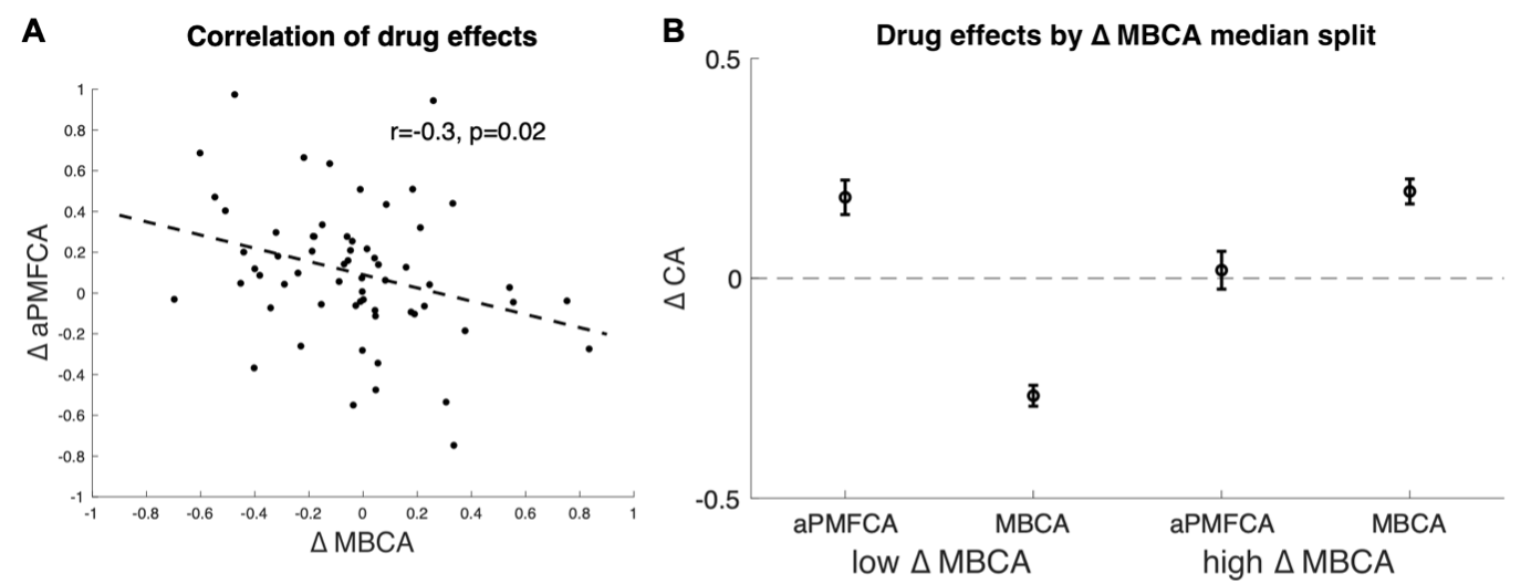
Figure 6. Inter-individual differences in drug effects in MBCA and in preferential MFCA, averaged across informative and non-informative destinations (aPMFCA). A) Scatter plot of the drug effects (levodopa minus placebo; ∆ aPMFCA, ∆ MBCA). Dashed regression line and r Pearson correlation coefficient. B) Drug effects in credit assignment (∆ CA) based on a median on ∆ MBCA. Error bars correspond to SEM reflecting variability between participants.
As suggested by the reviewer, we unpack this correlation further (p. 19/20) by taking the median on Δ MBCA (-0.019) and split the sample in lower/higher median groups. The higher median group showed a positive (M= 0.197, t(30)= 4.934, p<.001) and the lower-median group showed a negative (M= -0.267, t(30)= -7.97, p<.001) drug effect on MBCA, respectively (Figure 6B). In a mixed effects model (see Methods), we regressed aPMFCA against drug and a group indicator of lower/higher median Δ MBCA groups. This revealed a significant drug x Δ MBCA-split interaction (b=-0.17, t(120)=-2.05, p=0.042). In the negative Δ MBCA group (Figure 6B), a significantly positive drug effect on aPMFCA was detected (simple effect: b=.18, F(120,1)=10.35, p=.002) while in the positive Δ MBCA group a drug-dependent change in aPMFCA was not significant (Figure 6B, simple effect: b=.02, F(120,1)=0.10, p=.749).
We have changed the respective section of the results accordingly (p. 19/20). Further, we have motivated this exploratory analysis more clearly in the introduction (p. 3/4) in terms of it providing a link to previous relevant studies (Deserno et al., 2015a; Groman et al., 2019; Sharp et al., 2016; Wunderlich et al., 2012). Lastly, we have endeavoured to improve the discussion on this (p. 21/22).
More generally I would recommend that the authors refrain from putting too much emphasis on these between-subject correlations. Simple power calculation indicates that the sample size one would need to detect a realistically small to medium between-subject effect (that interacts with all kinds of within-subject factors) is in any case much larger than the sample size in this study.
We agree with this and have, as mentioned above, substantially adjusted the section on inter-individual differences. We have moved the WM analysis to Appendix 1 (p. 44/45, subheading “Drug effect on guidance of MFCA and working memory”, Appendix 1 - Figure 11) and greatly simplified the analysis of inter-individual differences in drug effects (see previous paragraph). We also mention the overall small to moderate effects in the limitations section (p. 25/26).
Another question is how worried should we be that the critical MB guidance of MFCA effect was not observed under placebo (Figure 3b)? I realize that the computational model-based analyses do speak to this issue, but here I had some questions too. Are the results from the model-informed and model-agnostic analyses otherwise consistent? Model-agnostic analyses reveal a greater effect of LDopa on informative destination for the ghost-nominated than the ghost-rejected trials and no effect for noninformative destination. Conversely model-informed analyses reveal a nomination effect of ldopa across informative and noninformative trials. This was not addressed, or am I missing something? In fact, regarding the modeling, I am not the best person to evaluate the details of the model comparison, fitting and recovery procedures, but the question that does rise is, and I would make explicit in the current paper how does this model space, the winning model and the modeling exercise differ (or not) from that in the previous paper by Moran et al without LDopa administration.
A detailed response to this was provided in replay to point 6 as summarized by the editor. And we provide a summary here as well.
Firstly, we clearly indicate discrepancies between our model-agnostic and computational modelling analyse and acknowledge that discrepancies may be expected when effects of interest are weak to moderate, which we acknowledge (p. 25/26, limitations).
Secondly, the results from the computational model are generally statistically stronger, which is not surprising given that they are based on influences from far more trials. We now include a discussion of this in more detail in the section on limitations (p. 25/26).
Thirdly, although the computational model uses a slightly different parameterization from that reported in Moran et al. (2019), it is a formal extension of that model, allowing the strength of effects for informative and uninformative destinations to differ. We now include a reference to this change in parameterization in the limitation section (p. 25/26), and include a more detailed description in Appendix 1 (p. 45-47).
Finally, to test if the current models support our main conclusion from Moran et al. (2019) that retrospective MB inference guides MFCA for both the informative and non-informative destinations, we reanalysed the Moran et al. (2019) data using the current novel models and found converging support, as we now report (Appendix 1 – Figure 8).
Finally, the general story that dopamine boosts model-based instruction about what the model-free system should learn is reminiscent of the previous work showing that prefrontal dopamine alters instruction biasing of reinforcement learning (Doll and Frank) and I would have thought this might deserve a little more attention, earlier on in the intro.
The reviewer is indeed correct and we now reference this line of work (Doll et al., 2009, 2011) in the intro (p. 4).
Author Response
Reviewer #1 (Public Review):
While the mechanism about arm-races between plant and specialist herbivores has been studied, such as detoxification of specific secondary metabolites, the mechanism of the wider diet breadth, so-called generalist herbivores have been less studied. Since the heterogeneity of host plant species, the experimental validation of phylogenetic generalism of herbivores seemed as hard to be conducted. The authors declared the two major hypotheses about the large diet breadth ("metabolic generalism" and "multi-host metabolic specialism"), and carefully designed the experiment using Drosophila suzukii as a model herbivore species.
By an untargeted metabolomics approach using UHPLC-MS, authors attempted to falsify the hypotheses both in qualitative- and quantitative metabolomic profiles. Intersections of four fruit (puree) samples and each diet-based fly individual samples from the qualitative data revealed that there were few ions that occur as the specific metabolite in each diet-based fly group, which could reject the "multi-host metabolic specialism" hypothesis. Quantitative data also showed results that could support the "metabolic generalism" hypothesis. Therefore, the wide diet breadth of D. suzukii seemed to be derived from the general metabolism rather than the adaptive traits of the diverse host plant species. On the other hand, the reduction of the metabolites (ions) set using GLM seemed logical and 2-D clustering from the reduced ions set showed that quantitative aspects of diet-associated ions could classify "what the flies ate". These interesting results could enhance the understanding of the diet breadth (niche) of herbivorous insects.
The authors' approach seemed clear to falsify the hypotheses based on the appropriate data processing. The intersection of shared ions from the qualitative dataset could distinguish the diet-specific metabolites in flies and commonly occurring metabolites among flies and/or fruits. Also, filtering on the diet-specific ions seemed to be a logical and appropriate way. Meanwhile, the discussion about the results seemed to be focused on different points regarding the research hypotheses which were raised in the introduction part. Discussion about the results mainly focused on the metabolism of D. suzukii itself, rather than the research hypotheses and questions that were raised from the evolution of the wide diet breadth of generalist herbivores. In particular, the conclusion seems to be far from the main context of the authors' research; e.g. frugivory. It makes the implication of the study weaker.
We wish to thank Reviewer #1 for their appreciation of our study. As recommended, we now focus our discussion more on the general aspect of our findings (relevant to insects, herbivores, or frugivores), and less on the peculiarities of the metabolism of D. suzukii itself. Specifically, we now only mention D. suzukii in one section (two sentences) of our Discussion, to serve as an example (l.387-396). Thanks to this comment, the Discussion may interest a broader readership, on the evolution of diet breadth in generalist herbivorous species and offers a better understanding of the general implications of our findings.
Reviewer #2 (Public Review):
The manuscript: "Metabolic consequences of various fruit-based diets in a generalist insect species" by Olazcuaga et al., addresses an interesting question. Using an untargeted metabolomics approach, the authors study how diet generalism may have evolved versus diet specialization which is generally more commonly observed, at least in drosophila species. Using the phytophagous species Drosophila suzukii, and by directly comparing the metabolomes of fruit purees and the flies that fed on them, the authors found evidence for "metabolic generalism". Metabolic generalism means that individuals of a generalist species process all types of diet in a similar way, which is in contrast to "multi-host metabolic specialism" which entails the use of specific pathways to metabolize unique compounds of different diets. The authors find strong evidence for the first hypothesis, as they could easily detect the signature of each fruit diet in the flies. The authors then go on to speculate on the evolutionary ramifications of this for how potentially diet specializations may have evolved from diet generalism. Overall, the paper is well written, the experiments well documented, and the conclusions convincing.
We thank Reviewer #2 for their comments and appreciation of our work.
Reviewer #3 (Public Review):
Laure Olazcuaga et al. investigated the metabolomes of four fruit-based diets and corresponding individuals of Drosophila suzukii that reared on them using comparative metabolomics analysis. They observed that the four fruit-based diets are metabolically dissimilar. On the contrary, flies that fed on them are mostly similar in their metabolic response. From a quantitative point of view, they find that part of the fly metabolomes correlates well with that of the corresponding diet metabolomes, which is indicative of insect ingestive history. By further focusing on 71 metabolites derived from diet-specific fly ions and highly abundant fruit ions, the authors show that D. suzukii differentially accumulates diet metabolism in a compound-specific manner. The authors claim that the data support the metabolic generalism hypothesis while rejecting the multi-host metabolic specialism hypothesis. This study provides a valuable global chemical comparison of how diverse diet metabolites are processed by a generalist insect species.
Strengths:
The rapid advances in high-resolution mass spectrometry have recently accelerated the discovery of many novel post-ingestive compounds through comparative metabolomics analysis of insect/frass and plant samples. Untargeted metabolomics is thus a very powerful approach for the systematic comparison of global chemical shifts when diverse plant-derived specialized metabolites are further modified or quantitatively metabolized after ingestion by insects. The technique can be readily extended to a larger micro- or macro-evolutionary context for both generalist and specialist insects to systematically investigate how plant chemical diversity contributes to dietary generalism and specialism.
We would like to thank Reviewer #3 for their insightful comments on the power of untargeted metabolomics to evaluate the fate of plant metabolites and their use by herbivores. We also agree that these techniques can be used to tackle eco-evolutionary issues, such as the origin and maintenance of dietary generalism and specialism here. We hope that our study will inspire other researchers to explore such techniques and experiments to gain a global overview of biochemistry fluxes and their evolution. We now mention it in the conclusion (L454-459).
Weaknesses:
The authors claim that their data support the hypothesis of metabolic generalism, however, a total analysis of insect metabolism may not generate a clean dataset for direct comparison of fruit-derived metabolites with those metabolized by D. suzukii, given that much of these metabolites would be "diluted" proportionally by insect-derived metabolites. If the insect-derived metabolites predominate, then, as the authors observed, a tight clustering of D. suzukii metabolomes in the PCA plot would be expected. It is therefore very difficult to interpret these patterns.
We agree with Reviewer #3 that a careful examination of the different possible origins of metabolites should take place to distinguish between our two competing hypotheses.
The only source of metabolites for insects in our experimental setup is a mixture of (i) a large proportion of fruit purees and (ii) a minor proportion of artificial medium consisting mainly of yeast. Our goal is thus to understand the fate of (i) “fruit-derived” metabolites (transformed and untransformed), while controlling for (ii) “artificial media-derived” metabolites, that constitute a nuisance signal but are necessary for a complete development in our system.
By “fruit-derived” and “insect-derived” metabolites, it is our understanding that Reviewer #3 means “fruit” metabolites (when in insects, untransformed “fruit-derived” metabolites) and “artificial medium-derived” metabolites. It is true that we do wish to avoid a predominance of “artificial medium-derived” metabolites and focus on “fruit-derived” metabolites in insects. We also want to note that it is of primary importance in our study to distinguish between “fruit” metabolites that are carried as is (“fruit” metabolites present in insects, ie untransformed “fruit-derived” metabolites), and “fruit” metabolites that are used after transformation by the insect (i.e., transformed “fruit-derived” metabolites).
We agree with Reviewer #3 that the presence of “artificial medium-derived” metabolites could be problematic in direct comparisons of fruits and insects (and not among fruits or among insects’ comparisons).
However, we took some steps to avoid such problems:
We included control fly samples in our experiment: at each experimental generation, flies developed only on artificial medium (without fruit puree) were collected and processed simultaneously with flies that developed on fruit media. Results using these artificial medium-reared flies as controls (by subtracting their ions levels and removing ions that were similar, respective of their generation) were similar to results using raw data and conclusions were identical (see below).
We lowered the proportion of artificial medium in our fruit media so that it was kept to a minimum, compatible with larval development and adult survival.
Consistent with the low impact of this “artificial medium” component on our conclusions, we also wish to point out the presence pattern of metabolites found only in flies and never in fruits when using raw data (Figure 3, yellow stack). Even in the most conservative hypothesis of 100% of these metabolites originating from our artificial medium (which is probably not the case), we observe that it constitutes only a minor proportion of metabolites common to all flies (15.7%).
For your consideration, we include below the main Figures, using both raw data and artificial medium-controlled:
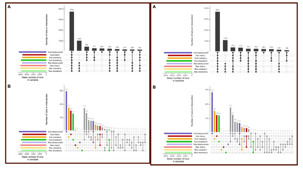
Figure 2, left = raw data; right = artificial-media controlled:
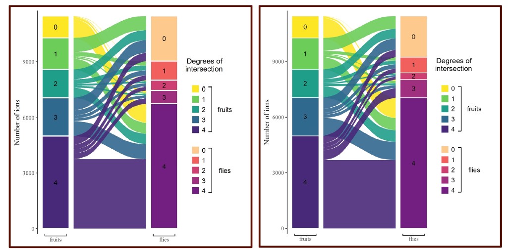
Figure 3, left = raw data; right = artificial-media controlled:
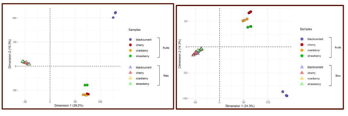
Figure 3S1, left = raw data; right = artificial-media controlled:
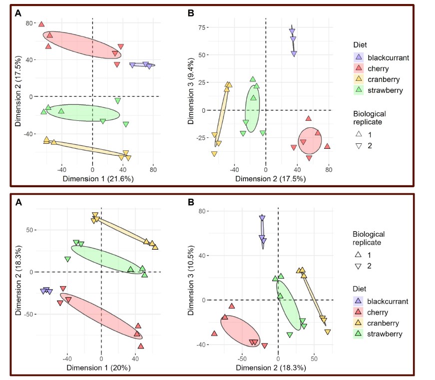
Figure 4, above = raw data; below = artificial-media controlled:
We hope that we convinced the Editor/Reviewers that raw data and artificial-medium controlled data provide a single and same answer to all our analyses. We chose to present only raw data, to simplify the Materials & Methods section.
We however modified the current version of the manuscript to inform the reader that proper controls were done and that their inclusion do not modify any of our conclusions (l.110-113 and l.583-589).
We also wish to point out two additional comments:
As Reviewer #1 also recommended, we modified the expectations drawn in Fig1G to better consider the general comment of “insect derived” metabolites being fundamentally different from plant metabolites (even if we do show in our study that only approx. 9% of metabolites are private to flies).
The main part of our care in the use of this global PCA analysis is that it follows two other analyses (global intersection and comparison of intersections among fruits and among flies) and precedes another one (fly-focused PCA). We hope that all these analyses help the readers get a comprehensive overview of the dataset and associated results, avoiding reliance on a single analysis.
We also help readers to explore and visualize all analyses presented in our manuscript by setting up a shiny application (in addition to our available dataset and R code), at https://fruitfliesmetabo.shinyapps.io/shiny/. This is now mentioned in the main text (l.588-589).
We thank the Reviewer for their comment that greatly improved the manuscript.
The authors generated a qualitative dataset using the peak list produced by XCMS which contains quantitative peak areas, it is unclear how the threshold was selected to determine if a peak is present or absent in a given sample. The qualitative dataset would influence the output of their data analysis.
The referee is right in pointing out that the threshold used to determine if a peak is present or absent in a given sample was not clearly specified. This has now been corrected in the “Host use” section of the Materials & Methods (l.513-516). Briefly, a given replicate of a compound was considered present if the corresponding peak area following XCMS quantification was > 1000. This threshold was selected to be close to the practical quantification threshold of the Thermo Exactive mass spectrometer used in this study. This threshold was selected in order to allow the quantification of low-abundance compounds, as many plant-derived diet compounds were expected to be present in trace amounts in flies. We additionally applied a stringent rule for presence of any given compound (presence in at least 3 biological replicates).
The authors reply on in-source fragmentation for peak annotation when authentic standards are not available. The accuracy of the annotation thus requires further validation.
The Supplementary Table 1 was unfortunately omitted in the first submission of the manuscript. This oversight has been now corrected and the Supplementary Table 1 details all information used for metabolite annotation. In particular, MS/MS data comparison with mass spectral databases as well as with published literature have been added to substantiate metabolite identifications. This MS/MS data was produced thanks to the comment of the Reviewer. We also provide four more annotations from standards to attain 30 / 71 identifications validated through chemical standards.
Author Response:
Reviewer #1 (Public Review):
This paper provides experimental and modeling analysis of the inter-brain coupling of socially interacting bats, and reports that coordinated brain activity evolves at a slower time scale than the activity describing the differences. Specifically, the paper finds that there is an attracting submanifold corresponding to the mean (or "common mode") of neural activity, and that the dynamics in the orthogonal eigenmode, corresponding to the difference in brain activity, decays rapidly. These rapid decays in the difference mode are referred to as "catch up" activity.
There are two main findings:
1) Neural activity (especially higher frequency LFP activity in the 30-150Hz range) is modulated by social context. Specifically, the ratio of the averaged, moment-to-moment MEAN:DIFF ratio is much higher when the bats are in a single chamber, clearly indicating that the animals are coordinating their neural activity. This change also seems to hold -- although not as striking -- in lower-frequency LFP and spiking activity.
2) The time scales of the mean vs. difference dynamics are segregated: the "difference dynamics" evolve at a faster time scale than "similarity dynamics", seems to be well supported.
The basic finding is presented in Figure 1. The rest of the paper is focused on a modeling study to garner further insight into the dynamics.
Weaknesses:
This is an entirely phenomenological paper, and while it claims to garner "mechanistic insight", it is unclear what that means.
We regret not clarifying sufficiently what we meant by “mechanistic insight.” The insight is the following: functional across-brain coupling acts as positive feedback to the mean component of neural activity, which amplifies it and slows it down; at the same time, it acts as negative feedback to the difference component, which suppresses it and speeds it up. Thus, findings (1) and (2) in the reviewer’s summary above can be explained by the same model mechanism. As the reviewer pointed out below, the details of the model are complex, which could have made the simple mechanism above opaque. Thus, we analyzed two simplified versions of the model to make the mechanistic insight clear. This is detailed below in our response to the reviewer’s comment on model complexity.
The basic idea of the model is simple and somewhat interesting, but the details are extremely complex. There are many examples of this, but the method used to "regress out" the behavior was very hard to interpret.
The method for regressing out behavior was described in Materials and Methods section 3.10, and we regret having neglected to reference it in the main text. We now reference it at the first instance in the main text where this is relevant.
On the face of it, the model is extremely simple: a two-state linear dynamical system. However, this simplistic description buries extreme complexity. The model is extremely complex as involves a large number of parameters (e.g., time switching 'b' values, the values of which are completely unclear), the switching over time of these parameters based on hand-scored animal behavioral state, and the complex mix of markovian and linear dynamical systems theoretic results.
As the reviewer pointed out, the core of the model is very simple: a linear dynamical system that models neural activity coupling. The model mechanism of positive and negative feedback, which is responsible for reproducing the two experimental results summarized by the reviewer above, is contained in this core (see Materials and Methods section 3.7 for details). On top of this, the model has a layer of complexity, involving a Markov chain model of behavior and a large number of behavioral parameters. This layer of complexity is independent from the feedback mechanism of the core of the model. Thus, while it makes the model more biologically realistic, it is not required to reproduce the two main experimental results. To explicitly show this, and to better understand the dependence of model behavior on its parameters, we analyzed two reduced versions of the model.
The first reduced model replaces the behavioral inputs with white noise. The original model is 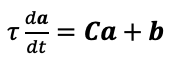 , where a is neural activity,
 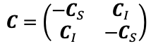 , is the coupling matrix, b is behavioral modulation, and τ is a time constant. b is where the complexity lies, as it is simulated using a Markov chain and involves many parameters. To strip away this layer of complexity, we replaced b with noise having a simple structure, namely, the mean and difference components of b having identical, flat power spectra. Importantly, this noise input does not induce correlation between bats, and it amounts to inputs of the same magnitude and same timescales to the mean and difference components of a.
The resulting reduced model has only two parameters, the functional self-coupling C_S and functional across-brain coupling C_I (for simplicity, τ can be absorbed into the other parameters). We are interested in the two results the reviewer summarized above: (1) the mean component of neural activity having a larger variance than the difference component; (2) the mean component having a slow timescale than the difference component. In the manuscript, these are respectively quantified using the variance ratio and the power spectral centroid ratio of the mean and difference components. The reduced model allowed us to derive analytical expressions for these two quantities (see Materials and Methods section 3.8 for details). We found that they have very simple dependence on the functional coupling parameters: the variance ratio (mean variance divided by difference variance) is approximately
, is the coupling matrix, b is behavioral modulation, and τ is a time constant. b is where the complexity lies, as it is simulated using a Markov chain and involves many parameters. To strip away this layer of complexity, we replaced b with noise having a simple structure, namely, the mean and difference components of b having identical, flat power spectra. Importantly, this noise input does not induce correlation between bats, and it amounts to inputs of the same magnitude and same timescales to the mean and difference components of a.
The resulting reduced model has only two parameters, the functional self-coupling C_S and functional across-brain coupling C_I (for simplicity, τ can be absorbed into the other parameters). We are interested in the two results the reviewer summarized above: (1) the mean component of neural activity having a larger variance than the difference component; (2) the mean component having a slow timescale than the difference component. In the manuscript, these are respectively quantified using the variance ratio and the power spectral centroid ratio of the mean and difference components. The reduced model allowed us to derive analytical expressions for these two quantities (see Materials and Methods section 3.8 for details). We found that they have very simple dependence on the functional coupling parameters: the variance ratio (mean variance divided by difference variance) is approximately  , and the centroid ratio (mean centroid divided by difference centroid) is approximately
  .
.
This parameter dependence is visualized below (note that the color maps are in log scale, and the white spaces are regions where the model is unstable).
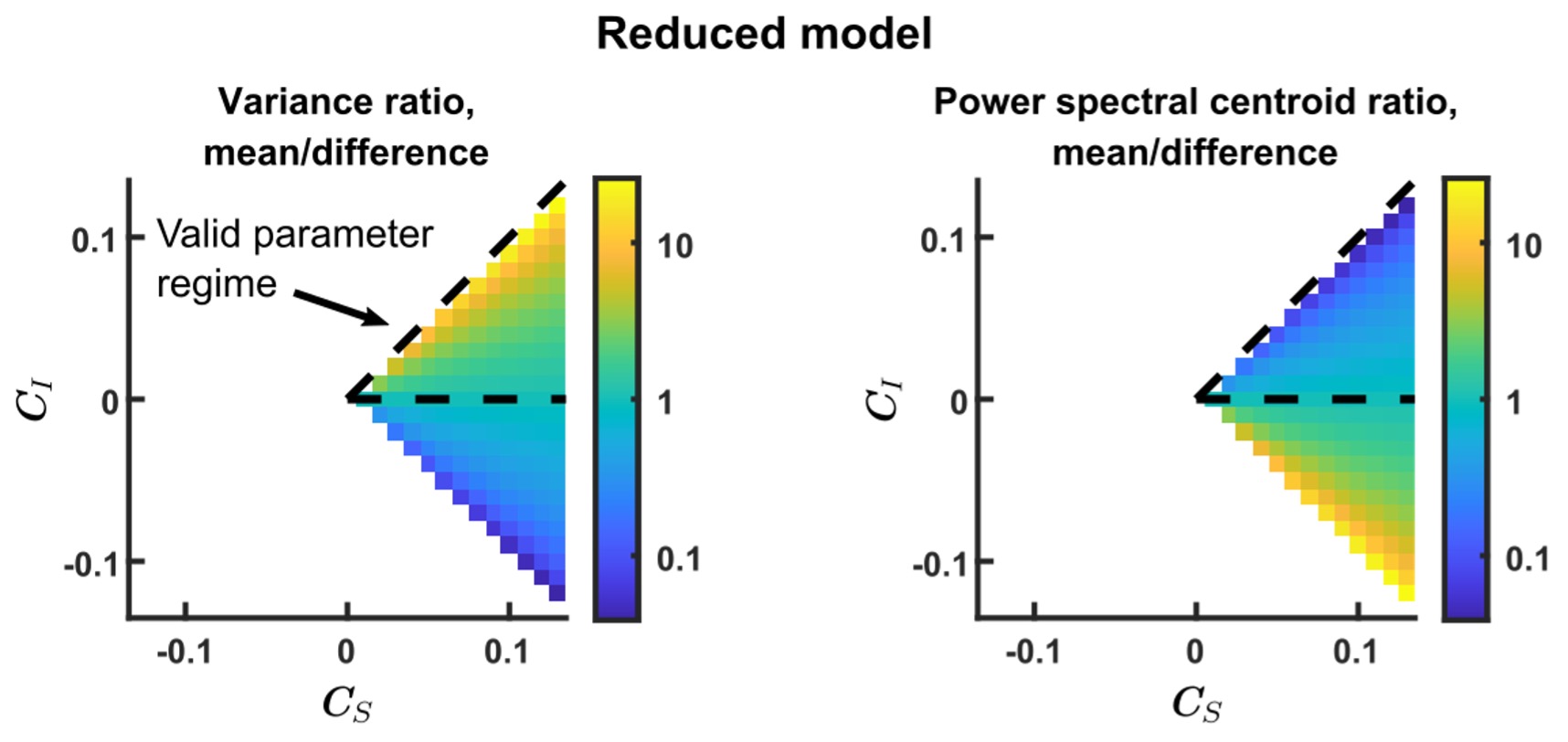
In the experimental data, the mean component had larger variance and lower power spectral centroid than the difference component. This corresponds to the parameter regime of  (enclosed by dashed lines). Thus, a positive C_I acts as positive feedback to the mean component and negative feedback to the difference component, modulating their variance and timescales in opposite directions. This is consistent with the analysis of the original model in Materials and Methods section 3.7. In the revised manuscript, we’ve now added analysis of this reduced model to the Results section, and the above figure has been added as Figure 3I-J.
The reviewer has stated a concern regarding the large number of parameters that set the input level according to behavioral state (b_resting, b_(social grooming), b_fighting, etc.). These parameters are important for ensuring that the model outputs realistic levels of behaviorally modulated neural activity (discussed below in our reply regarding model fit), but they are not important for the main results on variance and timescales. To demonstrate this, we studied a second reduced model. This model is identical to our original model except that, for each simulation, each of the behavior parameters (b_fighting, etc.) was independently drawn from the uniform distribution from 0 to 1. Despite the completely random behavioral parameters, this reduced model reproduces the variance and timescales results just like the original model, as shown in the figure below (compare with Figure 3E-F).
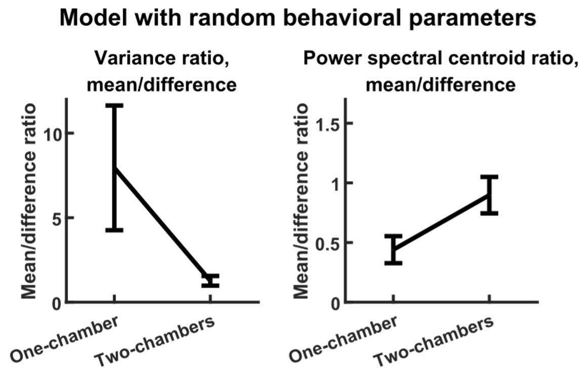
To summarize, the reduced models allowed us to identify the simple parameter dependence of the modeling results, and showed that the simple linear dynamical system at the core of the original model is sufficient to reproduce the two main experimental observations.
Indeed, a fundamental weakness of the model is that the Markov chain is taken as an "input" to the 2-state linear systems model, as if somehow the neural state does not affect the state transitions.
Yes, this is a limitation of our model. We’ve added a discussion of this limitation, as well as future directions for overcoming it, in the Discussion section. The reason we did not model neural control of behavioral transitions is that it is under-constrained by existing data. While the brain obviously controls behaviors, not every part of the brain controls every behavior. Of the 11 behaviors observed in this study, we do not know which of them is controlled by the bat frontal cortex, and we do not know how they might be controlled (i.e., what specific spatiotemporal activity patterns affects behaviors in what ways). Without this knowledge, it’s unclear how to implement neural control of behavior in the model. This knowledge requires perturbation studies (lesion, inactivation, or activity manipulation) to establish casual relationships from neural activity to specific behaviors in the bat, which will be an important future direction.
On the other hand, as the reviewer stated, our model included behavioral modulation of neural activity. It is well known that in mammals, arousal and movement modulate neural activity globally across cortex (McGinley et al., 2015, Neuron). Thus, given that different behaviors in general involve different levels of arousal and movement, our model included behavior-dependent modulation of frontal cortical neural activity. Finally, for the reviewer’s convenience, we also quote below the paragraph addressing this issue in the revised Discussion. “Another limitation of our model is the “open-loop” nature of the relationship between behavior and neural activity. Specifically, we modeled neural activity as being modulated by behavior, but behavior was modeled using a Markov chain that is independent from the neural activity. In reality, neural activity and behavior form a closed-loop, with different social behaviors being controlled by the neural activity of specific neural populations in specific brain regions. Thus, an important future direction is to close the loop by incorporating neural control of social behaviors into models of the inter-brain relationship in bats. This will require future experimental studies to identify which frontal cortical regions and populations in bats are necessary or sufficient to control social behaviors, as well as the detailed causal relationship from neural activity to social behavior. Furthermore, as social interactions can occur at multiple timescales, it will be interesting to investigate how these are controlled by neural activity at different timescales, and how those timescales are shaped by functional across-brain coupling. In summary, such a closed-loop model will shed light on how inter-brain activity patterns and dynamic social interactions co-evolve and feedback onto each other.”
Further, the Markov assumption is not rigorously tested.
We have now tested the Markov assumption, using the following methods. We compared three models of bat behaviors: (1) the independent model, where the behavioral state at a given time point is independent from the state at other time points; (2) the 1st-order dependency model, where the behavioral state at a given time point depends on the state at the previous time point only; (3) the 2nd-order dependency model, where the behavioral state at a given time point depends on the states at the two previous time points. The Markov assumption corresponds to model (2), which is used as a part of the main model of the paper. Note that models with longer time-dependencies (≥3) were not tested because the number of parameters grows exponentially with model order and our dataset is not large enough to fit them.
To compare the three models, we split the behavioral data into a training set and a test set, fitted each model on the training set (Laplace smoothing was used to avoid assigning zero probability to unobserved events), and calculated the log-likelihood of the test set under each model. The figure below shows the cross-validated likelihoods for the behavioral data of one-chamber (A) and two-chambers (B) sessions, which were fitted separately; circles and error bars are means and standard deviations across 100 random splits of the data into training and test sets.
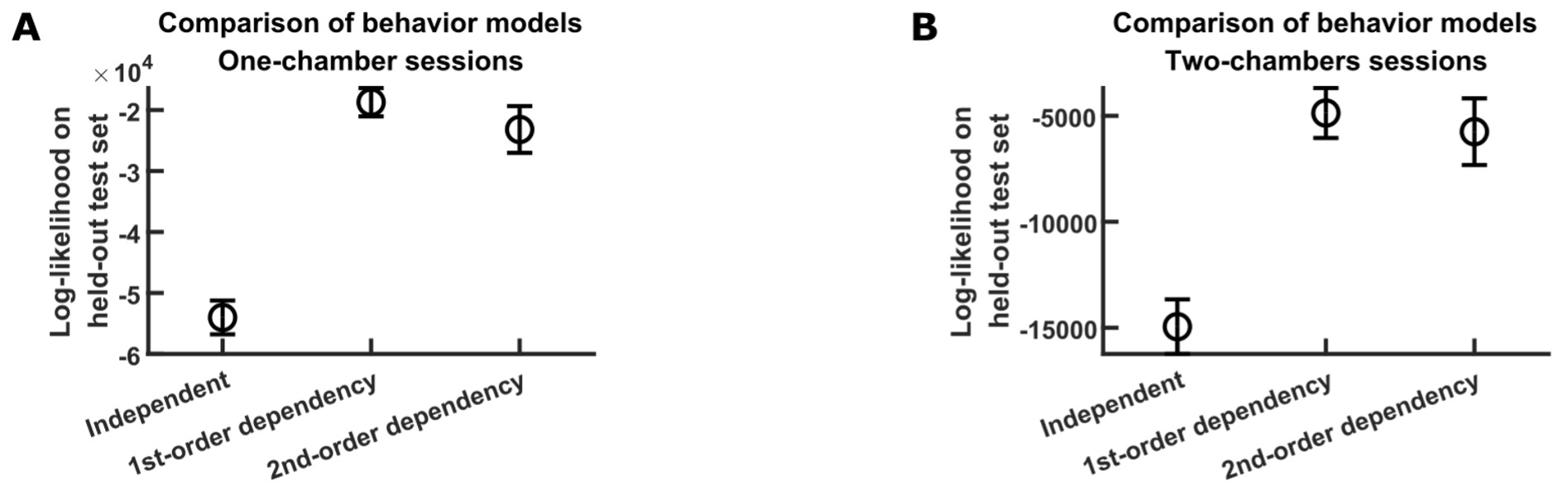
As the figure above shows, the 1st-order model had the highest likelihood on average. This does not necessarily prove that bat behavior obeys the Markov assumption (if we had a lot more data, we might be able to fit better 2nd-order and higher-order models). But this does mean that, given the amount of data we have, the best model that we can fit is the 1st-order Markov chain. Thus, this result supports our usage of the Markov chain in the main model of the paper. In the revised manuscript, the above figure is included as Figure 3—figure supplement 2A-B, and the analysis is described in Materials and Methods section 3.5.
No model selecting or other model validation appears to be done.
To evaluate model fit, we simulated our model using experimentally observed behaviors (rather than simulating behaviors using a Markov chain), and compared the simulated neural activity with the experimentally observed activity (see Materials and Methods section 3.6 for detailed procedures). The comparison for an example experimental session is shown below, where we’ve plotted the experimentally observed neural activity and behaviors for bat 1 (A) and bat 2 (B), along with the simulated neural activity. The correlation coefficient between data and model are indicated above each plot. These are representative examples, as the average correlation over all sessions and bats is 0.72 (standard deviation is 0.10). This figure was added to the revised manuscript as Figure 3—figure supplement 1.
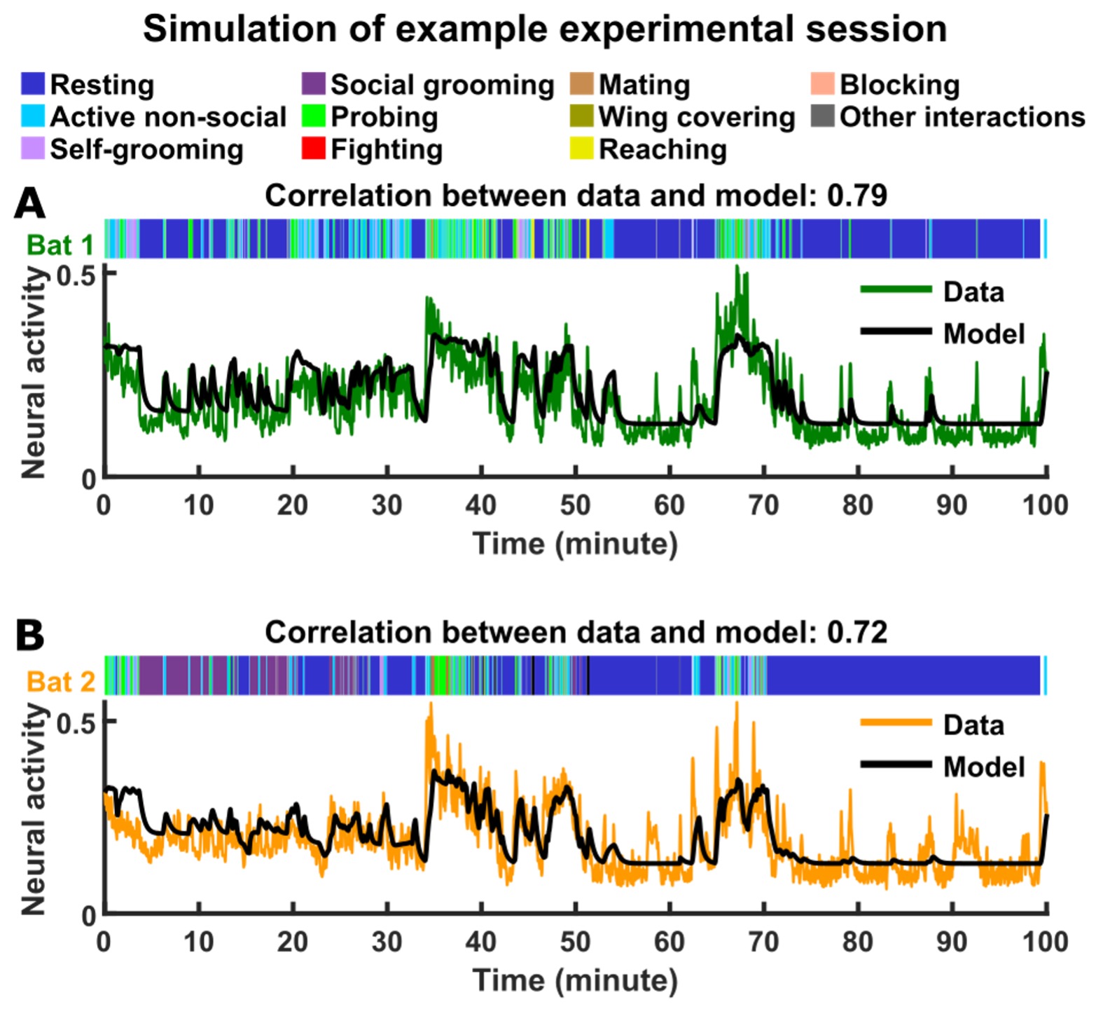
In evaluating model fit, we realized that the model in the original manuscript produced outputs with a DC offset different from that of the data. Thus, in the revised manuscript (including the figure above), we added one more behavioral parameter (b_constant) that adjusts the DC offset, which is a parameter that reflects the effect of a baseline arousal level on neural activity (Materials and Methods section 3.4). Note that, since the only effect of this parameter is to adjust the DC offset of neural activity, it does not change any of the results in the paper.
In short, the model, while very interesting, is so complex that it is literally impossible to evaluate. The authors report literally no shortcomings of their model. They do not report parameter estimation methods. They do not report fitting errors or other model validation metrics. The only evaluation is whether it can produce certain outputs that are similar to biological data. While the latter is certainly important, all models are wrong, and it essential to have a model simple enough to understand, both in terms of how it works and how it fails.
The comments on the complexity of the model and on fitting errors have been addressed above. Regarding parameter estimation methods, they were described in Materials and Methods section 3.14, and we regret having neglected to directly reference it in the original manuscript. We now reference the section in the legend of Figure 3A which is the first place to introduce the parameters. Briefly, the behavioral parameters (b_resting, b_fighting, etc.) were simply chosen to be the average neural activity during the respective behaviors from the data; the other parameters were chosen by hand to roughly match the levels of activity from the data, keeping within the parameter regime of  identified from the analyses. As we showed above, these parameters provide a reasonable fit to the data.
The reason we chose the parameters heuristically in this way, rather than by minimizing some error objective, is the following. Our goal was to build a model that could qualitatively reproduce the experimental findings in a robust manner, that is, without fine-tuning of parameters. Thus, we analyzed the model to understand how model behaviors depend on the parameters, and to identify the parameter regime that reproduces the qualitative trends seen in the data (Figure 3I-J; Materials and Methods sections 3.7 and 3.8). Guided by these analyses, we chose parameters heuristically without algorithmic fine-tuning.
Finally, following suggestions from reviewer 1 and reviewer 3, we have added discussions of shortcomings of the models (the last two paragraphs of the Discussion). With these discussions of model limitations, along with the presentation of simple insights into model mechanism from the reduced models above, we believe we have now presented a model that is “simple enough to understand, both in terms of how it works and how it fails.”
In general, while the basic finding is fairly interesting, and the experiments and their findings are highly relevant to the field, the modeling and its explication fall short.
It is not that it is wrong or bad; however, it is not clear that such a complex model increases our understanding beyond the experimental findings in Figure 1, and if it does, there has to be a major caveat that the model itself is not carefully vetted.
Based on the reviewer’s comments on the model’s complexity, we have analyzed reduced versions of the model to understand its simple underlying mechanisms, as described above. This goes beyond the experimental findings in Figure 1, as it provides a computational mechanism that could give rise to those experimental findings. Moreover, based on the reviewer’s comments, we have more carefully vetted the model, by evaluating model fit and testing different behavioral models that assume or doesn’t assume the Markov property. Finally, we now discuss caveats of the model in the Discussion section, including the open-loop nature of the model as pointed out by the reviewer.
Author Response
Reviewer #1 (Public Review):
Overall, the science is sound and interesting, and the results are clearly presented. However, the paper falls in-between describing a novel method and studying biology. As a consequence, it is a bit difficult to grasp the general flow, central story and focus point. The study does uncover several interesting phenomena, but none are really studied in much detail and the novel biological insight is therefore a bit limited and lost in the abundance of observations. Several interesting novel interactions are uncovered, in particular for the SPS sensor and GAPDH paralogs, but these are not followed up on in much detail. The same can be said for the more general observations, eg the fact that different types of mutations (missense vs nonsense) in different types of genes (essential vs non-essential, housekeeping vs. stress-regulated...) cause different effects.
This is not to say that the paper has no merit - far from it even. But, in its current form, it is a bit chaotic. Maybe there is simply too much in the paper? To me, it would already help if the authors would explicitly state that the paper is a "methods" paper that describes a novel technique for studying the effects of mutations on protein abundance, and then goes on to demonstrate the possibilities of the technology by giving a few examples of the phenomena that can be studied. The discussion section ends in this way, but it may be helpful if this was moved to the end of the introduction.
We modified the manuscript as suggested.
Reviewer #2 (Public Review):
Schubert et al. describe a new pooled screening strategy that combines protein abundance measurements of 11 proteins determined via FACS with genome-wide mutagenesis of stop codons and missense mutations (achieved via a base editor) in yeast. The method allows to identify genetic perturbations that affect steady state protein levels (vs transcript abundance), and in this way define regulators of protein abundance. The authors find that perturbation of essential genes more often alters protein abundance than of nonessential genes and proteins with core cellular functions more often decrease in abundance in response to genetic perturbations than stress proteins. Genes whose knockouts affected the level of several of the 11 proteins were enriched in protein biosynthetic processes while genes whose knockouts affected specific proteins were enriched for functions in transcriptional regulation. The authors also leverage the dataset to confirm known and identify new regulatory relationships, such as a link between the SDS amino acid sensor and the stress response gene Yhb1 or between Ras/PKA signalling and GAPDH isoenzymes Tdh1, 2, and 3. In addition, the paper contains a section on benchmarking of the base editor in yeast, where it has not been used before.
Strengths and weaknesses of the paper
The authors establish the BE3 base editor as a screening tool in S. cerevisiae and very thoroughly benchmark its functionality for single edits and in different screening formats (fitness and FACS screening). This will be very beneficial for the yeast community.
The strategy established here allows measuring the effect of genetic perturbations on protein abundances in highly complex libraries. This complements capabilities for measuring effects of genetic perturbations on transcript levels, which is important as for some proteins mRNA and protein levels do not correlate well. The ability to measure proteins directly therefore promises to close an important gap in determining all their regulatory inputs. The strategy is furthermore broadly applicable beyond the current study. All experimental procedures are very well described and plasmids and scripts are openly shared, maximizing utility for the community.
There is a good balance between global analyses aimed at characterizing properties of the regulatory network and more detailed analyses of interesting new regulatory relationships. Some of the key conclusions are further supported by additional experimental evidence, which includes re-making specific mutations and confirming their effects on protein levels by mass spectrometry.
The conclusions of the paper are mostly well supported, but I am missing some analyses on reproducibility and potential confounders and some of the data analysis steps should be clarified.
The paper starts on the premise that measuring protein levels will identify regulators and regulatory principles that would not be found by measuring transcripts, but since the findings are not discussed in light of studies looking at mRNA levels it is unclear how the current study extends knowledge regarding the regulatory inputs of each protein.
See response to Comment #10.
Specific comments regarding data analysis, reproducibility, confounders
1) The authors use the number of unique barcodes per guide RNA rather than barcode counts to determine fold-changes. For reliable fold changes the number of unique barcodes per gRNA should then ideally be in the 100s for each guide, is that the case? It would also be important to show the distribution of the number of barcodes per gRNA and their abundances determined from read counts. I could imagine that if the distribution of barcodes per gRNA or the abundance of these barcodes is highly skewed (particularly if there are many barcodes with only few reads) that could lead to spurious differences in unique barcode number between the high and low fluorescence pool. I imagine some skew is present as is normal in pooled library experiments. The fold-changes in the control pools could show whether spurious differences are a problem, but it is not clear to me if and how these controls are used in the protein screen.
Because of the large number of screens performed in this study (11 proteins, with 8 replicates for each) we had to trade off sequencing depth and power against cell sorting time and sequencing cost, resulting in lower read and barcode numbers than what might be ideally aimed for. As described further in the response to Comment #5, we added a new figure to the manuscript that shows that the correlation of fold-changes between replicates is high (Figure 3–S1A). The second figure below shows that the correlation between the number of unique barcodes and the number of reads per gRNA is highly significant (p < 2.2e-16).
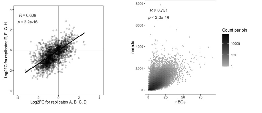
2) I like the idea of using an additional barcode (plasmid barcode) to distinguish between different cells with the same gRNA - this would directly allow to assess variability and serve as a sort of replicate within replicate. However, this information is not leveraged in the analysis. It would be nice to see an analysis of how well the different plasmid barcodes tagging the same gRNA agree (for fitness and protein abundance), to show how reproducible and reliable the findings are.
We agree with the reviewer that this would be nice to do in principle, but our sequencing depth for the sorted cell populations was not high enough to compare the same barcode across the low/unsorted/high samples. See also our response to Comment #5 for the replicate analyses.
3) From Fig 1 and previous research on base editors it is clear that mutation outcomes are often heterogeneous for the same gRNA and comprise a substantial fraction of wild-type alleles, alleles where only part of the Cs in the target window or where Cs outside the target window are edited, and non C-to-T edits. How does this reflect on the variability of phenotypic measurements, given that any barcode represents a genetically heterogeneous population of cells rather than a specific genotype? This would be important information for anyone planning to use the base editor in future.
We agree with the reviewer that the heterogeneity of editing outcomes is an important point to keep in mind when working with base editors. In genetic screens, like the ones described here, often the individual edit is less important, and the overall effects of the base editor are specific/localized enough to obtain insights into the effects of mutations in the area where the gRNA targets the genome. For example, in our test screens for Canavanine resistance and fitness effects, in which we used gRNAs predicted to introduce stop codons into the CAN1 gene and into essential genes, respectively, we see the expected loss-of-function effect for a majority of the gRNAs (canavanine screen: expected effect for 67% of all gRNAs introducing stop codons into CAN1; fitness screen: expected effect for 59% of all gRNAs introducing stop codons into essential genes) (Figure 2). In the canavanine screen, we also see that gRNAs predicted to introduce missense mutations at highly conserved residues are more likely to lead to a loss-of-function effect than gRNAs predicted to introduce missense mutations at less conserved residues, further highlighting the differentiated results that can be obtained with the base editor despite the heterogeneity in editing outcomes overall. We would certainly advise anyone to confirm by sequencing the base edits in individual mutants whenever a precise mutation is desired, as we did in this study when following up on selected findings with individual mutants.
4) How common are additional mutations in the genome of these cells and could they confound the measured effects? I can think of several sources of additional mutations, such as off-target editing, edits outside the target window, or when 2 gRNA plasmids are present in the same cell (both target windows obtain edits). Could some of these events explain the discrepancy in phenotype for two gRNAs that should make the same mutation (Fig S4)? Even though BE3 has been described in mammalian cells, an off-target analysis would be desirable as there can be substantial differences in off-target behavior between cell types and organisms.
Generally, we are not very concerned about random off-target activity of the base editor because we would not expect this to cause a consistent signal that would be picked up in our screen as a significant effect of a particular gRNA. Reproducible off-target editing with a specific gRNA at a site other than the intended target site would be problematic, though. We limited the chance of this happening by not using gRNAs that may target similar sequences to the intended target site in the genome. Specifically, we excluded gRNAs that have more than one target in the genome when the 12 nucleotides in the seed region (directly upstream of the PAM site) are considered (DiCarlo et al., Nucleic Acids Research, 2013).
We do observe some off-target editing right outside the target window, but generally at much lower frequency than the on-target editing in the target window (Figure 1B and Figure 1–S2). Since for most of our analyses we grouped perturbations per gene, such off-target edits should not affect our findings. In addition, we validated key findings with independent experiments. For our study, we used the Base Editor v3 (Komor et al., Nature, 2016); more recently, additional base editors have been developed that show improved accuracy and efficiency, and we would recommend these base editors when starting a new study (see, e.g., Anzalone et al., Nature Biotechnology, 2020).
We are not concerned about cases in which one cell gets two gRNAs, since the chance that the same two gRNAs end up in one cell repeatedly is low, and such events would therefore not result in a significant signal in our screens.
We don’t think that off-target mutations can explain the discrepancy between pairs of gRNAs that should introduce the same mutation (Figure 3–S1. The effect of the two gRNAs is actually well-correlated, but, often, one of the two gRNAs doesn’t pass our significance cut-off or simply doesn’t edit efficiently (i.e., most discrepancies arise from false negatives rather than false positives). We may therefore miss the effects of some mutations, but we are unlikely to draw erroneous conclusions from significant signals.
5) In the protein screen normalization uses the total unique barcode counts. Does this efficiently correct for differences from sequencing (rather than total read counts or other methods)? It would be nice to see some replicate plots for the analysis of the fitness as well as the protein screen to be able to judge that.
We made a new figure that shows a replicate comparison for the protein screen (see below; in the manuscript it is Figure 3–S1A) and commented on it in the manuscript. For this analysis, the eight replicates for each protein were split into two groups of four replicates each and analyzed the same way as the eight replicates. The correlation between the two groups of replicates is highly significant (p < 2.2e-16). The second figure shows that the total number of reads and the total number of unique barcodes are well correlated.
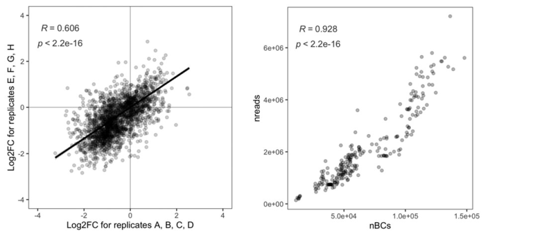
For the fitness screen, we used read counts rather than barcode counts for the analysis since read counts better reflect the dropout of cells due to reduced fitness. The figure below shows a replicate comparison for the fitness screen. For this analysis, the four replicates were split into two groups of two replicates each and analyzed the same way as the four replicates. The correlation between the two groups of replicates is highly significant (p < 2.2e-16).
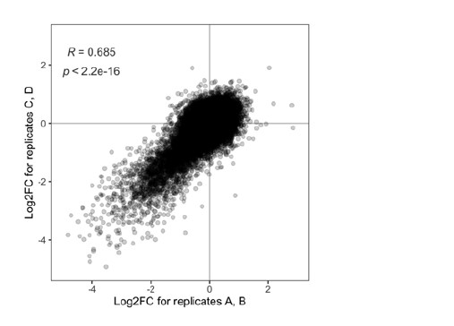
6) In the main text the authors mention very high agreement between gRNAs introducing the same mutation but this is only based on 20 or so gRNA pairs; for many more pairs that introduce the same mutation only one reaches significance, and the correlation in their effects is lower (Fig S4). It would be better to reflect this in the text directly rather than exclusively in the supplementary information.
We clarified this in the manuscript main text: “For 78 of these gRNA pairs, at least one gRNA had a significant effect (FDR < 0.05) on at least one of the eleven proteins; their effects were highly correlated (Pearson’s R2 = 0.43, p < 2.2E-16) (Figure 3–S1B). For the 20 gRNA pairs for which both gRNAs had a significant effect, the correlation was even higher (Pearson’s R2 = 0.819, p = 8.8e-13) (Figure 3–S1C). These findings show that the significant gRNA effects that we identify have a low false positive rate, but they also suggest that many real gRNA effects are not detected in the screen due to limitations in statistical power.”
7) When the different gRNAs for a targeted gene are combined, instead of using an averaged measure of their effects the authors use the largest fold-change. This seems not ideal to me as it is sensitive to outliers (experimental error or background mutations present in that strain).
We agree that the method we used is more sensitive to outliers than averaging per gene. However, because many gRNAs have no effect either because they are not editing efficiently or because the edit doesn’t have a phenotypic consequence, an averaging method across all gRNAs targeting the same gene would be too conservative and not properly capture the effect of a perturbation of that gene.
8) Phenotyping is performed directly after editing, when the base editor is still present in the cells and could still interact with target sites. I could imagine this could lead to reduced levels of the proteins targeted for mutagenesis as it could act like a CRISPRi transcriptional roadblock. Could this enhance some of the effects or alter them in case of some missense mutations?
To reduce potential “CRISPRi-like” effects of the base editor on gene expression, we placed the base editor under a galactose-inducible promoter. For both the fitness and protein screens we grew the cultures in media without galactose for another 24 hours (fitness screen) or 8-9 hours (protein screens) before sampling. In the latter case, this recovery time corresponded to more than three cell divisions, after which we assume base editor levels to have strongly decreased, and therefore to no longer interfere with transcription. This is also supported by our ability to detect discordant effects of gRNAs targeting the same gene (e.g., the two mutations leading to loss-of-function and gain-of-function of RAS2), which would otherwise be overshadowed by a CRISPRi effect.
9) I feel that the main text does not reflect the actual editing efficiency very well (the main numbers I noticed were 95% C to T conversion and 89% of these occurring in a specific window). More informative for interpreting the results would be to know what fraction of the alleles show an edit (vs wild-type) and how many show the 'complete' edit (as the authors assume 100% of the genotypes generated by a gRNA to be conversion of all Cs to Ts in the target window). It would be important to state in the main text how variable this is for different gRNAs and what the typical purity of editing outcomes is.
We now show the editing efficiency and purity in a new figure (Figure 1B), and discuss it in the main text as follows: “We found that the target window and mutagenesis pattern are very similar to those described in human cells: 95% of edits are C-to-T transitions, and 89% of these occurred in a five-nucleotide window 13 to 17 base pairs upstream of the PAM sequence (Figure 1A; Figure 1–S2) (Komor et al., 2016). Editing efficiency was variable across the eight gRNAs and ranged from 4% to 64% if considering only cases where all Cs in the window are edited; percentages are higher if incomplete edits are considered, too (Figure 1B).”
Comments regarding findings
10) It would be nice to see a comparison of the results to the effects of ~1500 yeast gene knockouts on cellular transcriptomes (https://doi.org/10.1016/j.cell.2014.02.054). This would show where the current study extends established knowledge regarding the regulatory inputs of each protein and highlight the importance of directly measuring protein levels. This would be particularly interesting for proteins whose abundance cannot be predicted well from mRNA abundance.
We agree with the reviewer that it would be very interesting to compare the effect of perturbations on mRNA vs protein levels. We have compared our protein-level data to mRNA-level data from Kemmeren and colleagues (Kemmeren et al., Cell 2014), and we find very good agreement between the effects of gene perturbations on mRNA and protein levels when considering only genes with q < 0.05 and Log2FC > 0.5 in both studies (Pearson’s R = 0.79, p < 5.3e-15).
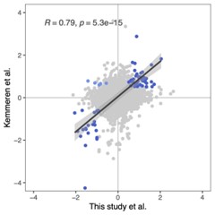
Gene perturbations with effects detected only on mRNA but not protein levels are enriched in genes with a role in “chromatin organization” (FDR = 0.01; as a background for the analysis, only the 1098 genes covered in both studies were considered). This suggests that perturbations of genes involved in chromatin organization tend to affect mRNA levels but are then buffered and do not lead to altered protein levels. There was no enrichment of functional annotations among gene perturbations with effects on protein levels but not mRNA levels.
We did not include these results in the manuscript because there are some limitations to the conclusions that can be drawn from these comparisons, including that our study has a relatively high number of false negatives, and that the genes perturbed in the Kemmeren et al. study were selected to play a role in gene regulation, meaning that differences in mRNA-vs-protein effects of perturbations are limited to this function, and other gene functions cannot be assessed.
11) The finding that genes that affect only one or two proteins are enriched for roles in transcriptional regulation could be a consequence of 'only' looking at 10 proteins rather than a globally valid conclusion. Particularly as the 10 proteins were selected for diverse functions that are subject to distinct regulatory cascades. ('only' because I appreciate this was a lot of work.)
We agree with this, and we think it is clear in the abstract and the main text of the manuscript that here we studied 11 proteins. We made this point also more explicit in the discussion, so that it is clear for readers that the findings are based on the 11 proteins and may not extrapolate to the entire yeast proteome.
Reviewer #3 (Public Review):
This manuscript presents two main contributions. First, the authors modified a CRISPR base editing system for use in an important model organism: budding yeast. Second, they demonstrate the utility of this system by using it to conduct an extremely high throughput study the effects of mutation on protein abundance. This study confirms known protein regulatory relationships and detects several important new ones. It also reveals trends in the type of mutations that influence protein abundances. Overall, the findings are of high significance and the method appears to be extremely useful. I found the conclusions to be justified by the data.
One potential weakness is that some of the methods are not described in main body of the paper, so the reader has to really dive into the methods section to understand particular aspects of the study, for example, how the fitness competition was conducted.
We expanded the first section for better readability.
Another potential weakness is the comparison of this study (of protein abundances) to previous studies (of transcript abundances) was a little cursory, and left some open questions. For example, is it remarkable that the mutations affecting protein abundance are predominantly in genes involved in translation rather than transcription, or is this an expected result of a study focusing on protein levels?
We thank the reviewer for pointing out that this paragraph requires more explanation. We expanded it as follows: “Of these 29 genes, 21 (72%) have roles in protein translation—more specifically, in ribosome biogenesis and tRNA metabolism (FDR < 8.0e-4, Figure 5C). In contrast, perturbations that affect the abundance of only one or two of the eleven proteins mostly occur in genes with roles in transcription (e.g., GO:0006351, FDR < 1.3e-5). Protein biosynthesis entails both transcription and translation, and these results suggest that perturbations of translational machinery alter protein abundance broadly, while perturbations of transcriptional machinery can tune the abundance of individual proteins. Thus, genes with post-transcriptional functions are more likely to appear as hubs in protein regulatory networks, whereas genes with transcriptional functions are likely to show fewer connections.”
Overall, the strengths of this study far outweigh these weaknesses. This manuscript represents a very large amount of work and demonstrates important new insights into protein regulatory networks.
Author Response
Reviewer #2 (Public Review):
The authors seek to determine how various species combine their effects on the growth of a species of interest when part of the same community.
To this end, the authors carry out an impressive experiment containing what I believe must be one of the largest pairwise + third-order co-culture experiments done to date, using a high-throughput co-culture system they had co-developed in previous work. The unprecedented nature of this data is a major strength of the paper. The authors also discover that species combine their effect through "dominance", i.e. the strongest effect masks the others. This is important as it calls into question the common assumption of additivity that is implicit in the choice of using Lotka-Volterra models.
A stronger claim (i.e. in the abstract) is that joint effect of multiple species on the growth of another can be derived from the effect of individual species. Unless I am misunderstanding something, this statement may have to be qualified a little, as the authors show that a model based on pairwise dominance (i.e. the strongest pairwise) does a somewhat better job (lower RMSD, though granted, not by much, 0.57 vs 0.63) than a model based on single species dominance. This is, the effect of the strongest pair predicts better the effect of a trio than the effect of the larger species.
This issue makes one wonder whether, had the authors included higher-order combinations of species (i.e. five-member consortia or higher), the strongest-effect trio would have predicted better than the strongest-effect pair, which in turn is better predictor than the strongest-effect species. This is important, as it would help one determine to what extent the strongest-effect model would work in more diverse communities, such as those one typically finds in nature. Indeed, the authors find that the predictive ability of the strongest effect species is much stronger for pairs than it is for trios (RMSD of 0.28 vs 0.63). Does the predictive ability of the single species model decline faster and faster as diversity grows beyond 4-member consortia?
Thank you for raising this important point. It is true that in our study we see that single species predict pairs better than trios, and that pairs predict trios better than single species. As we did not perform experiments on more diverse communities (n>4), we are not sure if or how these rules will scale up. We explicitly address these caveats in our revised discussion.
Reviewer #3 (Public Review):
A problem in synthetic ecology is that one can't brute-force complex community design because combinatorics make it basically impossible to screen all possible communities from a bank of possible species. Therefore, we need a way to predict phenomena in complex communities from phenomena in simple communities. This paper aims to improve this predictive ability by comparing a few different simple models applied to a large dataset obtained with the use of the author's "kchip" microfluidics device. The main question they ask is whether the effect of two species on a focal species is predicted from the mean, the sum, or the max of the effect of each single "affecting" species on the focal species. They find that the max effect is often the best predictor, in the sense of minimizing the difference between predicted effect and measured effect. They also measure single-species trait data for their library of strains, including resource niche and antibiotic resistance, and then find that Pearson correlations between distance calculations generated from these metrics and the effect of added species are weak and unpredictive. This work is largely well-done, timely and likely to be of high interest to the field, as predicting ecosystem traits from species traits is a major research aim.
My main criticism is that the main take-home from the paper (fig 3B)-that the strongest effect is the best predictor-is oversold. While it is true that, averaged over their six focal species, the "strongest effect" was the best overall predictor, when one looks at the species-specific data (S9), we see that it is not the best predictor for 1/3 of their focal species, and this fraction grows to 1/2 if one considers a difference in nRMSE of 0.01 to be negligible.
As suggested, we have softened our language regarding the take-home message. This matter is addressed in detail above in response to 'Essential Revisions'. Briefly, we see that the strongest model works best when both single species have qualitatively similar effects, but is slightly less accurate when effects are mixed. We also see overall less accurate predictions for positive effects. In light of these findings, we propose that focal species for which the strongest model is not the most accurate is due to the interaction types, and not specific to the focal species.
We made substantial changes to the manuscript, including the first paragraph of the discussion which more accurately describes these findings and emphasizes the relevant caveats:
"By measuring thousands of simplified microbial communities, we quantified the effects of single species, pairs, and trios on multiple focal species. The most accurate model, overall and specifically when both single species effects were negative, was the strongest effect model. This is in stark contrast to models often used in antibiotic compound combinations, despite most effects being negative, where additivity is often the default model (Bollenbach 2015). The additive model performed well for mixed effects (i.e. one negative and one positive), but only slightly better than the strongest model, and poorly when both species had effects of the same sign. When both single species’ effects were positive, the strongest model was also the best, though the difference was less pronounced and all models performed worse for these interactions. This may be due to the small effect size seen with positive effects, as when we limited negative and mixed effects to a similar range of effects strength, their accuracy dropped to similar values (Figure 3–Figure supplement 5). We posit that the difference in accuracy across species is affected mainly by the effect type dominating different focal species' interactions, rather than by inherent species traits (Figure 3–Figure supplement 6)." (Lines 288-304)
The same criticism applies to the result from figure 2-that pairs of affecting species have more negative effects than single species. Considered across all focal species this is true (though minor in effect size, Fig 2A). But there is only a significant effect within two individual species. Again, this points to the effects being focal-species-specific, and perhaps not as generalizable as is currently being claimed.
Upon more rigorous analysis, and with regard to changes in the dataset after filtering, we see that the more accurate statement is that effects become stronger, not necessarily more negative (in line with the accuracy of the strongest model). The overall trend is towards more negative interactions, due to the majority of interactions being negative, but as stated this is not true for each individual focal. As such the following sentence in the manuscript has been changed:
"The median effect on each focal was more negative by 0.28 on average, though the difference was not significant in all cases; additionally, focals with mostly positive single species interactions showed a small increase in median effect (Fig. 2D)" (Lines 151-154)
As well as the title of this section: "Joint effects of species pairs tend to be stronger than those of individual affecting species" (Lines 127-128)
Another thing that points to a focal-species-specific response is Fig 2D, which shows the distributions of responses of each focal species to pairs. Two of these distributions are unimodal, one appears bimodal, and three appear tri-modal. This suggests to me that the focal species respond in categorically different ways to species addition.
We believe this distribution of pair effects is related to the distribution of single species effects, and not to the way in which different focal species respond to the addition of second species. Though this may be difficult to see from the swarm plots shown in the paper, below is a split violin plot that emphasizes this point.
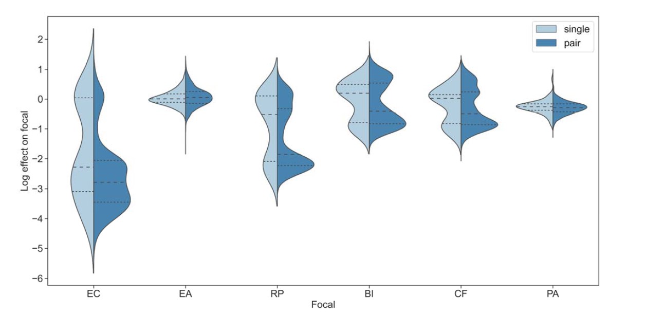
Fig R1: Distribution of single species and pair effects. Distribution of the effect of single and pairs of affecting species for each focal species individually. Dashed lines represent the median, while dotted lines the interquartile range.
These differences occur even though the focal bacteria are all from the same family. This suggests to me that the generalizability may be even less when a more phylogenetically dispersed set of focal species are used.
We have added the following sentence to the discussion explicitly emphasizing the phylogenetic limitations of our study:
"Lastly, it is important to note that our focal species are all from the same order (Enterobacterales), which may also limit the purview of our findings." (Lines 364-366)
Considering these points together, I argue that the conclusion should be shifted from "strongest effect is the best" to "in 3 of our focal species, strongest effect was the best, but this was not universal, and with only 6 focal species, we can't know if it will always be the best across a set of focal species".
As mentioned above, we have softened our language regarding the take-home message in response to these evaluations.
My second main criticism is that it is hard to understand exactly how the trait data were used to predict effects. It seems like it was just pearson correlation coefficients between interspecies niche distances (or antibiotic distances) and the effect. I'm not very surprised these correlations were unpredictive, because the underlying measurements don't seem to be relevant to the environment tested. What if, rather than using niche data across 20 nutrients, only the growth data on glucose (the carbon source in the experiments) was used? I understand that in a field experiment, for example, one might not know what resources are available, and so measuring niche across 20 resources may be the best thing to do. Here though it seems imperative to test using the most relevant data.
It is true that much of the profiling data is not directly related to the experimental conditions (different carbon sources and antibiotics), but in addition to these we do use measurements from experiments carried out in the same environment as the interactions assays (i.e. growth rate and carrying capacity when growing on glucose), which also showed poor correlation with the effects on focals. Additionally, we believe that these profiles contain relevant information regarding metabolic similarity between species (similar to metabolic models often constructed computationally). To improve clarity, we added the following sentence to the figure legend of Figure 3–Figure supplement 1:
"The growth rate, and maximum OD shown in panel A were measured only in M9 glucose, similar to conditions used in the interaction assays." (Lines 591-592)
Additionally and relatedly, it would be valuable to show the scatterplots leading to the conclusion that trait data were uninformative. Pearson's r only works on an assumption of linearity. But there could be strong relationships between the trait data and effect that are monotonic but not linear, or even that are non-monotonic yet still strong (e.g. U-shaped). For the first case, I recommend switching to Spearman's rho over Pearson's r, because it only assumes monotonicity, not linearity. If there are observable relationships that are not monotonic, a different test should be used.
Per your suggestion, we have changed the measurement of correlation in this analysis from Pearson's r, to Spearman's rho. As we observed similar, and still mostly weak correlations, we did not investigate these relationships further. See Figure 3–Figure supplement 1.
Additionally, we generated heat maps including scatterplots mapping the data leading to these correlations. We found no notable dependency in these plots, and visually they were quite crowded and difficult to interpret. As this is not the central point of our study, we ultimately decided against adding this information to the plots.
In general, I think the analyses using the trait data were too simplistic to conclude that the trait data are not predictive.
We agree that more sophisticated analyses may help connect between species traits and their effects on focal species. In fact, other members of our research group have recently used machine learning to accomplish similar predictions (https://doi.org/10.1101/2022.08.02.502471). As such we have changed the wording in to reflect that this correlation is difficult to find using simple analyses:
"These results indicate that it may be challenging to connect the effects of single and pairs of species on a focal strain to a specific trait of the involved strains, using simple analysis." (Lines 157-159)
Author Response
Reviewer #1 (Public Review):
Slusarczyk et al present a very well written manuscript focused on understanding the mechanisms underlying aging of erythrophagocytic macrophages in the spleen (RPM) and its relationship to iron loading with age. The manuscript is diffuse with a broad swath of data elements. Importantly, the manuscript demonstrates that RPM erythrophagocytic capacity is diminished with age, restored in iron restricted diet fed aged mice. In addition, the mechanism for declining RPM erythrophagocytic capacity appears to be ferroptosis-mediated, insensitive to heme as it is to iron, and occur independently of ROS generation. These are compelling findings. However, some of the data relies on conjecture for conclusion and a clear causal association is not clear. The main conclusion of the manuscript points to the accumulation of unavailable insoluble forms of iron as both causing and resulting from decreased RPM erythrophagocytic capacity.
We are proposing that intracellular iron accumulation progresses first and leads to global proteotoxic damage and increased lipid peroxidation. This eventually triggers the death of a fraction of aging RPMs, thus promoting the formation of extracellular iron-rich protein aggregates. More explanation can be found below. Besides, iron loading suppresses the erythrophagocytic activity of RPMs, hence further contributing to their functional impairment during aging.
In addition, the finding that IR diet leads to increased TF saturation in aged mice is surprising.
We believe that this observation implies better mobilization of splenic iron stores, and corroborates our conclusion that mice that age on an iron-reduced diet benefit from higher iron bioavailability, although these differences are relatively mild. More explanation can be found in our replies to Reviewer #2.
Furthermore, whether the finding in RPMs is intrinsic or related to RBC-related changes with aging is not addressed.
We now addressed this issue and we characterized in more detail both iron and ROS levels in RBCs.
Finally, these findings in a single strain and only female mice is intriguing but warrants tempered conclusions.
We tempered the conclusions and provided a basic characterization of the RPM aging phenotype in Balb/c female mice.
Major points:
1) The main concern is that there is no clear explanation of why iron increases during aging although the authors appear to be saying that iron accumulation is both the cause of and a consequence of decreased RPM erythrophagocytic capacity. This requires more clarification of the main hypothesis on Page 4, line 17-18.
We thank the reviewer for this comment. It was previously reported that iron accumulates substantially in the spleen during aging, especially in female mice (Altamura et al., 2014). Since RPMs are those cells that process most of the iron in the spleen, we aimed to explore what is the relationship between iron accumulation and RPM functions during aging. This investigation led us to uncover that indeed iron accumulation is both the cause and the consequence of RPM dysfunction. Specifically, we propose that intracellular iron loading of RPMs precedes extracellular deposition of iron in a form of protein-rich aggregates, driven by RPMs damage. To support this, we now show that the proteome of RPMs overlaps with those proteins that are present in the age-triggered aggregates (Fig. 3F). Furthermore, corroborating our model, we now demonstrate that transient iron loading of RPMs via iron-dextran injection (new Fig. 3G) leads to the formation of protein-rich aggregates, closely resembling those present in aged spleens (new Fig. 3H). This implies that high iron content in RPMs is indeed a major driving factor that leads to aggregation of their proteome and cell damage. Importantly, we now supported this model with studies using iRPMs. We demonstrated that iron loading and blockage of ferroportin by synthetic mini-hepcidin (PR73)(Stefanova et al., 2018) cause protein aggregation in iRPMs and lead to their decreased viability only in cells that were exposed to heat shock, a well-established trigger of proteotoxicity (new Fig. 5K and L). We propose that these two factors, namely age-triggered decrease in protein homeostasis and exposure to excessive iron levels, act in concert and render RPMs particularly sensitive to damage during aging (see also Discussion, p. 16).
In parallel, our data imply that the increased iron content in aged RPMs drives their decreased erythrophagocytic activity, as we now better documented by more extensive in vitro experiments in iRPMs (new Fig 6E-H). We cannot exclude that some of the senescent splenic RBCs that are retained in the red pulp and evade erythrophagocytosis due to RPM defects in aging, may also contribute to the formation of the aggregates. This is supported by the fact that mice that lack RPMs as well exhibit iron loading in the spleen (Kohyama et al., 2009; Okreglicka et al., 2021), and that the proteome of aggregates overlaps to some extent with the proteome of erythrocytes (new Fig. 3F).
We believe that during aging intracellular iron accumulation is chiefly driven by ferroportin downregulation, as also suggested by Reviewer#3. We now show that ferroportin drops significantly already in mice aged 4 and 5 months (new Fig. 4H), preceding most of the other impairments. This drop coincides with the increase in hepcidin expression, but if this is the sole reason for ferroportin suppression during early aging would require further investigation outside the scope of the present manuscript.
In sum, to address this comment, we now modified the fragment of the introduction that refers to our hypothesis and major findings to be more clear (p. 4), we improved our manuscript by providing new data mentioned above and we added more explanation in the corresponding sections of the Results and Discussion.
2) It is unclear if RPMs are in limited supply. Based on the introduction (page 4, line 13-15), they have limited self-renewal capacity and blood monocytes only partially replenished. Fig 4D suggests that there is a decrease in RPMs from aged mice. The %RPM from CD45+ compartment suggests that there may just be relatively more neutrophils or fewer monocytes recruited. There is not enough clarity on the meaning of this data point.
Thank you for this comment. We fully agree that %RPMs of CD45+ splenocytes, although well-accepted in literature (Kohyama et al., 2009; Okreglicka et al., 2021), is only a relative number. Hence, we now included additional data and explanations regarding the loss of RPMs during aging.
It was reported that the proportion of RPMs derived from bone marrow monocytes increases mildly but progressively during aging (Liu et al., 2019). This implies that due to the loss of the total RPM population, as illustrated by our data, the cells of embryonic origin are likely even more affected. We could confirm this assumption by re-analysis of the data from Liu et al. that we now included in the manuscript as Fig. 5E. These data clearly show that the representation of embryonically-derived RPMs drops more drastically than the percent of total RPMs, whereas the replenishment rate from monocytes is not affected significantly during aging. Consistent with this, we have not observed any robust change in the population of monocytes (F4/80-low, CD11b-high) or pre-RPMs (F4/80-high, CD11b-high) in the spleen at the age of 10 months (Figure 5-figure supplement 2A and B). We also have detected a mild decrease, not an increase, in the number of granulocytes (new Figure 5-figure supplement 2C). Furthermore, we measured in situ apoptosis marker and found a clear sign of apoptosis in the aged spleen (especially in the red pulp area), a phenotype that is less pronounced in mice on an IR diet (new Fig. 5O). This is consistent with the observation that apoptosis markers can be elevated in tissues upon ferroptosis induction (Friedmann Angeli et al., 2014) and that the proteotoxic stress in aged RPMs, which we now emphasized better in our manuscript, may also lead to apoptosis (Brancolini & Iuliano, 2020). Taken together, we strongly believe that the functional defect of embryonically-derived RPMs chiefly contributes to their shortage during aging.
3) Anemia of aging is a complex and poorly understood mechanistically. In general, it is considered similar to anemia of chronic inflammation with increased Epo, mild drop in Hb, and erythroid expansion, similar to ineffective erythropoiesis / low Epo responsiveness. It is not surprising that IR diet did not impact this mild anemia. However, was the MCV or MCH altered in aged and IR aged mice?
We now included the data for hematocrit, RBC counts, MCV, and MCH in Figure 1-figure supplement 5. Hematocrit shows a similar tendency as hemoglobin levels, but the values for RBC counts, MCV, and MCH seem not to be altered. We also show now that the erythropoietic activity in the bone marrow is not affected in aged versus young mice. Taken together, the anemic phenotype in female C57BL/6J mice at this age is very mild, which we emphasized in the main text, and is likely affected by other factors than serum iron levels (p. 6).
4) Page 6, line 23 onward: the conclusion is that KC compensate for the decreased function of RPM in the spleen, based on the expansion of KC fraction in the liver. Is there evidence that KCs are engaged in more erythrophagocytosis in aged mice? Furthermore, iron accumulation in the liver with age does not demonstrate specifically enhanced erythrophagocytosis of KC. Please clarify why liver iron accumulation would not be simply a consequence of increased parenchymal iron similar to increased splenic iron with age, independent of erythrophagocytic activity in resident macrophages in either organ.
Thanks for these questions. For the quantification of the erythrophagocytosis rate in KC, we show, as for the RPMs (Fig. 1K), the % of PKH67-positive macrophages, following transfusion of PKH67-stained stressed RBCs (Fig. 1M). The data implies a mild (not statistically significant) drop (of approx. 30%) in EP activity. We believe that it is overridden by a more pronounced (on average, 2-fold) increase in the representation of KCs (Fig. 1N). The mechanisms of iron accumulation between the spleen and the liver are very different. In the liver, we observed iron deposition in the parenchymal cells (not non-parenchymal, new Fig. 1P) that we currently characterizing in more detail in a parallel manuscript. Our data demonstrate a drop in transferrin saturation in aged mice. Hence, it is highly unlikely that aging would be hallmarked by the presence of circulating non-transferrin-bound iron that would be sequestered by hepatocytes, as shown previously (Jenkitkasemwong et al., 2015). Thus, the iron released locally by KCs is the most likely contributor to progressive hepatocytic iron loading during aging. The mechanism of iron delivery to hepatocytes from erythrophagocytosing KCs was demonstrated by Theurl et al.(Theurl et al., 2016), and we propose that it may be operational, although in a much more prolonged time scale, during aging. We now discussed this part better in our Results sections (p. 7).
5) Unclear whether the effect on RPMs is intrinsic or extrinsic. Would be helpful to evaluate aged iRPMs using young RBC vs. young iRPMs using old RBCs.
We are skeptical if the generation of iRPMs cells from aged mice would be helpful – these cells are a specific type of primary macrophage culture, derived from bone marrow monocytes with MCSF1, and exposed additionally to heme and IL-33 for 4 days. We do not expect that bone marrow monocytes are heavily affected by aging, and would thus recapitulate some aspects of aged RPMs from the spleen, especially after 8-day in vitro culture. However, to address the concerns of the reviewer, we now provide additional data regarding RBC fitness. Consistent with the time life-span experiment (Fig, 2A), we show that oxidative stress in RBCs is only increased in splenic, but not circulating RBCs (new Fig. 2C, replacing the old Fig. 2B and C). In addition, we show no signs of age-triggered iron loading in RBCs, either in the spleen (new Fig. 2F) or in the circulation (new Fig. 2B). Hence, we do not envision a possibility that RPMs become iron-loaded during aging as a result of erythrophagocytosis of iron-loaded RBCs. In support of this, we also have observed that during aging first RPMs’ FPN levels drop, afterward erythrophagocytosis rate decreases, and lastly, RBCs start to exhibit significantly increased oxidative stress (presented now in new Fig. 4H, J and K).
6) Discussion of aggregates in the spleen of aged mice (Fig 2G-2K and Fig 3) is very descriptive and non-specific. For example, if the iron-rich aggregates are hemosiderin, a hemosiderin-specific stain would be helpful. This data specifically is correlatory and difficult to extract value from.
Thanks for these comments. To the best of our knowledge Prussian blue Perls’ staining (Fig. 2J) is considered a hemosiderin staining. Our investigations aimed to better understand the nature and the origin of splenic iron deposits that to some extent are referred to as hemosiderin. Most importantly, as mentioned in our reply R1 Ad. 1. to assign causality to our data, we now demonstrated that iron accumulation in RPMs in response to iron-dextran (Fig. 3G) increases lipid peroxidation (Fig. 5F), tends to provoke RPMs depletion (Fig. 5G) and triggers the formation of protein-rich aggregates (new Fig. 3H). Of note, we assume that the loss of embryonically-derived RPMs in this model may be masked by simultaneous replenishment of the niche from monocytes, a phenomenon that may be addressed by future studies using Ms4a3-driven reporter mice (as shown for aged mice in our new Fig. 5E).
7) The aging phenotype in RPMs appears to be initiated sometime after 2 months of age. However, there is some reversal of the phenotype with increasing age, e.g. Fig 4B with decreased lipid peroxidation in 9 month old relative to 6 month old RPMs. What does this mean? Why is there a partial spontaneous normalization?
Thanks for this comment and questions. Indeed, the degree of lipid peroxidation exhibits some kinetics, suggestive of partial normalization. Of note, such a tendency is not evident for other aging phenotypes of RPMs, hence, we did not emphasize this in the original manuscript. However, in a revised version of the manuscript, we now present the re-analysis of the published data which implies that the number of embryonically-derived RPMs drops substantially between mice at 20 weeks and 36 weeks (new Fig. 5E). We think that the higher proportion of monocyte-derived RPMs in total RPM population later in aging (9 months) might be responsible for the partial alleviation of lipid peroxidation. We now discussed this possibility in the Results sections (p. 12).
8) Does the aging phenotype in RPMs respond to ferristatin? It appears that NAC, which is a glutathione generator and can reverse ferroptosis, does not reverse the decreased RPM erythrophagocytic capacity observed with age yet the authors still propose that ferroptosis is involved. A response to ferristatin is a standard and acceptable approach to evaluating ferroptosis.
We fully agree with the Reviewer that using ferristatin or Liproxstatin-1 would be very helpful to fully characterize a mechanism of RPMs depletion in mice. However, previous in vivo studies involving Liproxstatin-1 administration required daily injections of this ferroptosis inhibitor (Friedmann Angeli et al., 2014). This would be hardly feasible during aging. Regarding the experiments involving iron-dextran injection, using Liproxstatin-1 would require additional permission from the ethical committee which takes time to be processed and received. However, to address this question we now provide data from iRPMs cell cultures (new Fig.5 K-L). In essence, our results imply that both proteotoxic stress and iron overload act in concert to trigger cytotoxicity in RPM in vitro model. Interestingly, this phenomenon does not depend solely on the increased lipid peroxidation, but when we neutralize the latter with Liproxstatin-1, the cytotoxic effect is diminished (please, see also Results on p. 13 and Discussion p. 15/16).
9) The possible central role for HO-1 in the pathophysiology of decreased RPM erythrophagocytic capacity with age is interesting. However, it is not clear how the authors arrived at this hypothesis and would be useful to evaluate in the least whether RBCs in young vs. aged mice have more hemoglobin as these changes may be primary drivers of how much HO-1 is needed during erythrophagocytosis.
Thanks for this comment. We got interested in HO-1 levels based on the RNA sequencing data, which detected lower Hmox-1 expression in aged RPMs (Figure 3-figure supplement 1). We now show that the content of hemoglobin is not significantly altered in aged RBCs (MCH parameter, Figure 1-figure supplement 5E), hence we do not think that this is the major driver for Hmox-1 downregulation. Likewise, the levels of the Bach1 message, a gene encoding Hmox-1 transcriptional repressor, are not significantly altered according to RNAseq data. Hence, the reason for the transcriptional downregulation of Hmox-1 is not clear. Of note, HO-1 protein levels in the total spleen are higher in aged versus young mice, and we also detected a clear appearance of its nuclear truncated and enzymatically-inactive form (see a figure below, we opt not to include this in the manuscript for better clarity). The appearance of truncated HO-1 seems to be partially rescued by the IR diet. It is well established that the nuclear form of HO-1 emerges via proteolytic cleavage and migrates to the nucleus under conditions of oxidative stress (Mascaro et al., 2021). This additionally confirms that the aging spleen is hallmarked by an increased burden of ROS. Moreover, we also detected HO-1 as one of the components of the protein iron-rich aggregates. Thus, we propose that the low levels of the cytoplasmic enzymatically active form of HO-1 in RPMs (that we preferentially detect with our intracellular staining and flow cytometry) may be underlain by its nuclear translocation and sequestration in protein aggregates that evade antibody binding [this is also supported by our observation that the protein aggregates, despite the high content of ferritin (as indicated by MS analysis) are negative for L-ferritin staining. Of note, we also cannot exclude that other cell types in the aging spleen (eg. lymphocytes) express higher levels of HO-1 in response to splenic oxidative stress.
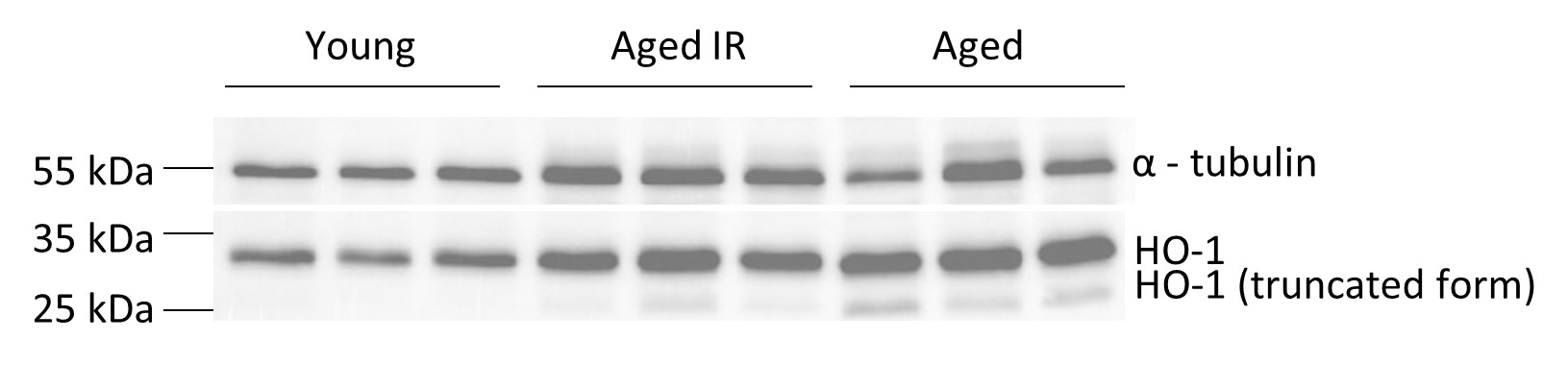
Fig. Total splenic levels of HO-1 in young, aged IR and aged mice.
Reviewer #2 (Public Review):
Slusarczyk et al. investigate the functional impairment of red pulp macrophages (RPMs) during aging. When red blood cells (RBCs) become senescent, they are recycled by RPMs via erythrophagocytosis (EP). This leads to an increase in intracellular heme and iron both of which are cytotoxic. The authors hypothesize that the continuous processing of iron by RPMs could alter their functions in an age-dependent manner. The authors used a wide variety of models: in vivo model using female mice with standard (200ppm) and restricted (25ppm) iron diet, ex vivo model using EP with splenocytes, and in vitro model with EP using iRPMs. The authors found iron accumulation in organs but markers for serum iron deficiency. They show that during aging, RPMs have a higher labile iron pool (LIP), decreased lysosomal activity with a concomitant reduction in EP. Furthermore, aging RPMs undergo ferroptosis resulting in a non-bioavailable iron deposition as intra and extracellular aggregates. Aged mice fed with an iron restricted diet restore most of the iron-recycling capacity of RPMs even though the mild-anemia remains unchanged.
Overall, I find the manuscript to be of significant potential interest. But there are important discrepancies that need to be first resolved. The proposed model is that during aging both EP and HO-1 expression decreases in RPMs but iron and ferroportin levels are elevated. In their model, the authors show intracellular iron-rich proteinaceous aggregates. But if HO-1 levels decrease, intracellular heme levels should increase. If Fpn levels increase, intracellular iron levels should decrease. How does LIP stay high in RPMs under these conditions? I find these to be major conflicting questions in the model.
We thank the Reviewer for her/his valuable feedback. As we mentioned in our replies we can only assume that a small misunderstanding in the interpretation of the presented data underlies this comment. We show that ferroportin levels in RPMs (Fig. 1F) are modulated in a manner that fully reflects the iron status of these cells (both labile and total iron levels, Figs. 1H and I). FPN levels drop in aged RPMs and are rescued when mice are maintained on a reduced iron diet. As pointed out by Reviewer#3, and explained in our replies we believe that ferroportin levels are critical for the observed phenotypes in aging. We now described our data in a more clear way to avoid any potential misinterpretation (p.6).
Reviewer #3 (Public Review):
This is a comprehensive study of the effects of aging of the function of red pulp macrophages (RPM) involved in iron recycling from erythrocytes. The authors document that insoluble iron accumulates in the spleen, that RPM become functionally impaired, and that these effects can be ameliorated by an iron-restricted diet. The study is well written, carefully done, extensively documented, and its conclusions are well supported. It is a useful and important addition for at least three distinct fields: aging, iron and macrophage biology.
The authors do not explain why an iron-restricted diet has such a strong beneficial effect on RPM aging. This is not at all obvious. I assume that the number of erythrocytes that are recycled in the spleen, and are by far the largest source of splenic iron, is not changed much by iron restriction. Is the iron retention time in macrophages changed by the diet, i.e. the recycled iron is retained for a short time when diet is iron-restricted (making hepcidin low and ferroportin high), and long time when iron is sufficient (making hepcidin high and ferroportin low)? Longer iron retention could increase damage and account for the effect. Possibly, macrophages may not empty completely of iron before having to ingest another senescent erythrocyte, and so gradually accumulate iron.
We are very grateful to this Reviewer for emphasizing the importance of the iron export capacity of RPMs as a possible driver of the observed phenotypes. Indeed, as mentioned above, we now show in the revised version of the manuscript that ferroportin drops early during aging (revised Fig. 4). Importantly, we now also observed that iron loading and limitation of iron export from iRPMs via ferroportin aggravate the impact of heat shock (a well-accepted trigger of proteotoxicity) on both protein aggregation and cell viability (new Fig. 5K and L). Physiologically, recent findings show that aging promotes a global decrease in protein solubility [BioRxiv manuscript (Sui X. et al., 2022)], and it is very likely that the constant exposure of RPMs to high iron fluxes renders these specialized cells particularly sensitive to proteome instability. This could be further aggravated by a build-up of iron due to the drop of ferroportin early during aging, ultimately leading to the appearance of the protein aggregates as early as at 5 months of age in C57BL/6J females. Based on the new data, we emphasized this model in the revised version of the manuscript (please, see Discussion on p. 16)
Author Response:
Reviewer #2:
Cai & Padoa-Schioppa recorded from macaque dorsal anterior cingulate cortex (ACCd) while requiring animals to choose between different juice types offered in variable amounts and with different action costs. Authors compared neural activity in ACCd (present study) with previous, directly comparable, findings on this same task when recording in macaque orbitofrontal cortex. The behavioral task is very powerful and the analyses of both the choice behavior and neural data are rigorous. Authors conclude that ACCd is unique in representing more post-decision variables and in its encoding of chosen value and binary outcome in several reference frames (chosen juice, chosen cost, and chosen action), not offer value, like OFC. Indeed, the encoding of choice outcomes in ACCd was skewed toward a cost-based reference frame. Overall, this is important new information about primate ACCd. I have only a few suggestions to enhance clarity. Figures 5 and 7 are maximally informative, but it is not clear that Figure 6 adds much to the reported Results. It is also suggested to abbreviate the comparison with Hosokawa et al. as it presently takes up 3 paragraphs in the Discussion: it is clear the methods and task designs were different enough to not be so easily compared with the present study. An additional suggestion would be to include mention of the comparison with OFC in the abstract and possibly also in the title, since the finding and direct comparison in Figure 7 are some of the most novel and interesting effects of the paper. Other suggestions are minor, and have to do with definition of time windows, variables, and additional papers that authors may cite for a well-rounded Discussion.
Please refer to Essential Revisions point #4. And we added “In contrast to the OFC” in the abstract to highlight the difference between these two regions.
Essential Revisions Point #4 Response:
We shortened the discussion from 3 paragraphs to 1 paragraph as follows.
"In another study, Hosokawa, Kennerley et al. (2013) compared the neuronal coding in ACCd and OFC in a choice task involving cost-benefit tradeoff. Our findings differ in two aspects. First, Hosokawa et. al. (2013) reported contralateral action value coding in ACCd while we did not discover significant offer value coding in either spatial- or action-based reference frames in our ACCd recordings. Second, they reported that there was no action-based value representation in the OFC therefore concluded that OFC does not integrate action cost in economic choice. Two elements may help explain the discrepancies between our findings in ACCd and OFC (Cai and Padoa-Schioppa 2019) and those of Hosokawa et. al. (2013). First, we recall that Hosokawa et. al. (2013) only tested value-related variables such as the benefit, cost and discounted value in action-based reference frame. Most importantly, they did not test the variable that is related to the saccade direction, which is highly correlated with the spatial value signal. As a consequence, contralateral value signal may not be significant if chosen target location was included in their regression analysis. Indeed, in our analysis, saccade direction (or chosen target location) was identified as one of the variables that explained a significant portion of neuronal activity in ACCd (Cai and Padoa-Schioppa 2012, Cai and Padoa-Schioppa 2019).The second and often overlooked aspect is that value may be encoded in schemes other than the action-based reference frame. In their study, each unique combination of reward quantity and cost was presented by a unique picture. Thus, information on good attributes were conveyed to the animal with an “integrated” visual representation. Accordingly, a distinct group of neurons may have been recruited to encode the reward and cost conjunctively represented by a unique fractal, which would result in 16 groups of offer value coding neurons."
Reviewer #3:
Cai and Padoa-Schioppa present a paper titled 'Neuronal Activity in Dorsal Anterior Cingulate Cortex during Economic Choices under Variable Action Costs'. They used a binary choice task where both offers indicated the reward type, reward amount, and the action cost (but not the specific action.) Variable action costs were then operationalized by placing targets on concentric circles of different radius. Here, and in a previous study that included OFC recordings (Cai and Padoa-Schioppa, 2019), monkeys integrated action costs into their decisions. Single-unit recordings in ACCd revealed that neurons predominantly coded for post-decision variables, such as cost of the chosen target and the juice type of the chosen offer, but not pre-decision variables, such as offer values. Given this finding, the authors compared the percentage of neurons in OFC and ACCd that coded for decision variables. In OFC neurons, the activity was mostly restricted to the offer presentation phase, whereas ACCd neurons showed sustained coding of chosen value and costs that lasted until the appearance of the saccade targets. Overall, this is an interesting study that provides evidence that decision-related signals evolve from coding offer values in the OFC to representing chosen costs in the ACC. This finding could highlight the roles of ACC neurons in learning and decision making. We have only a few questions.
1) Do any of the variables used in this study correlate with a conflict? When the authors previously studied ACC, they discarded the conflict monitoring hypothesis - a hypothesis that is well established for ACC hemodynamic responses - for ACC single cell activity based on neural data from 'difficult' decisions (Cai and Padoa-Schioppa, 2012). The definition of difficulty they used, then, was descriptive and based on reaction times (RTs). They defined the most difficult trials as those trials with the longest RTs and discovered that those trials had options with similar offer values. This definition of choice difficulty appears to be contrived from evidence accumulation models/tasks, where normatively harder judgments elicit longer RTs. However, there is no normative economic reason that trials with similar offer values are more difficult or should cause conflict. After all, according to theory, choosing between two options with the same value is as easy as flipping a coin. Here, it seems like the authors could have a more fitting definition of conflict. For example, conflict can be operationalized by considering trials when the animal must choose between a high value/high-cost option and a low-value/low-cost option. In that case, the costs and benefits are in conflict. What do the RTs look like? Do the RTs indicate conflict resolution? If so, is this reflected in neuronal responses?
We thank the reviewer for raising this important point. First, we would like to clarify that both in this study and in our previous study of ACC (Cai and Padoa-Schioppa 2012) we imposed a delay between offer presentation and the go signal. Such delay is critical to disentangle value comparison from action selection. However, the delay effectively dissociates reaction times from the decision difficulty. Normally, we operationalize the decision difficulty (or conflict) with the variable value ratio = chosen value / unchosen value. In an early behavioral study conducted in capuchin monkeys, where no delay was imposed between offer presentation and the go signal, we found that reaction times were strongly correlated with the value ratio, as one would naturally expect (Padoa-Schioppa, Jandolo et al. 2006). In the previous study of ACC (Cai and Padoa-Schioppa 2012) we referenced that earlier result but, again, we did not analyze reaction times.
Coming to the present study, we addressed this question by including in the variable selection analyses the two variables value ratio and cost/benefit conflict = cost of A * sign(offer value A – offer value B) (see also Table 2). The results of the updated analysis are illustrated in the new Figure 4, which we include here below. In essence, including these two variables did not affect the results of the variable selection analysis. That is, both the stepwise and best-subset methods selected the variables chosen value, chosen cost, chosen juice, chosen offer location only and chosen target location only.
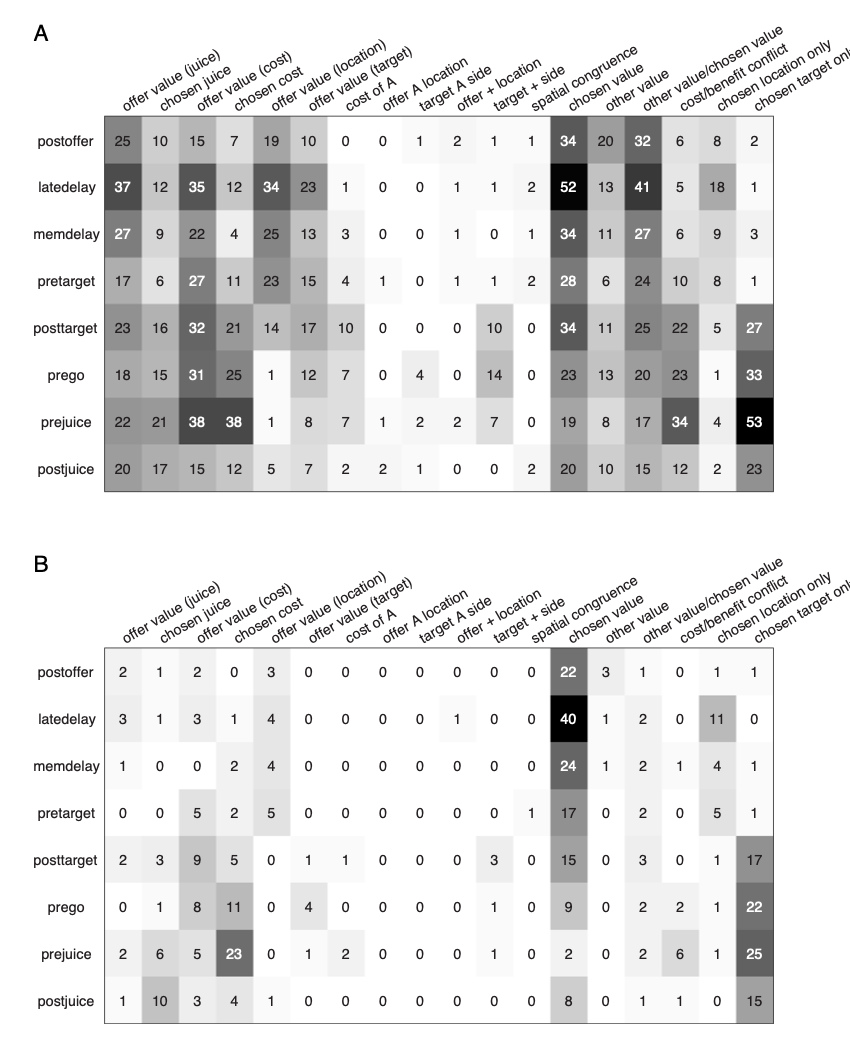
Figure 4. Population summary of ANCOVA (all time windows). (A) Explained responses. Row and columns represent, respectively, time windows and variables. In each location, the number indicates the number of responses explained by the corresponding variable in that time window. For example, chosen value (juice) explained 34 responses in the post-offer time window. The same numbers are also represented in gray scale. Note that each response could be explained by more than one variable and thus could contribute to multiple bins in this panel. (B) Best fit. In each location, the number indicates the number of responses for which the corresponding variable provided the best fit (highest R2 in that time window. For example, chosen value (juice) provided the best fit for 40 responses in the late-delay time window. The numerical values are also represented in gray scale. In this plot, each response contributes to at most one bin.
2) The authors claimed that the ACCd neurons integrated juice identity, juice quantity and action costs later in the trial. As they acknowledge, the evidence for this claim is marginal. The conclusion the authors made in line 211, therefore, could be moderated. Given that the model containing cost-related variables is more complex, it is equally valid and more appropriately to write '… we cannot reject the null hypothesis that action cost was not integrated by chosen value responses later in the trial.
We acknowledge the complexity of this claim. However, results from previous studies (Kennerley, Dahmubed et al. 2009, Kennerley and Wallis 2009, Hosokawa, Kennerley et al. 2013) are in favor of establishing a null hypothesis of integration rather than non-integration. Therefore, we feel that it is more appropriate to keep the null hypothesis of cost integration while in the meantime acknowledging that in our study the evidence for cost integration is rather weak.
Author Response
Reviewer #1 (Public Review):
1) It would be helpful to include some sort of comparison in Fig. 4, e.g. the regressions shown in Fig 3, to indicate to what extent the ICCl data corresponds to the "control range" of frequency tuning.
Figure 4 was modified to show the frequency range typically found in the ICCls. This range is based on results from Wagner et al., 2007, which extensively surveyed ICCls responses. This modification shows that our ICCls recordings in the ruff-removed owls cover the normal frequency hearing range of the owl.
2) A central hypothesis of the study is that the frequency preference of the high-frequency neurons is lower in ruff-removed owls because of the lowered reliability caused by a lack of the ruff. Yet, while lower, the frequency range of many neurons in juvenile and ruff-removed owls seems sufficiently high to be still responsive at 7-8 kHz. I think it would be important to know to what extent neurons are still ITD sensitive at the "unreliable high frequencies" even if the CFs are lower since the "optimization" according to reliability depends not on the best frequency of each neuron per se, but whether neurons are less ITD sensitive at the higher, less reliable frequencies.
The concern regarding the frequency range that elicits responsivity was largely addressed above. Specifically, Figure L1 showing frequency tuning of frontally tuned ICx neurons in ruff-removed owls indicates that while there is some variability of tuning across neurons, there is little responsivity above 6 kHz. In contrast, equivalent analysis in juvenile owls (Figure L3), shows there is much more responsiveness and variability across neurons to high and low frequencies. This evidence supports our hypothesis that the juvenile owl brain is still highly plastic, which facilitates learning during development. Although the underlying data was already reported in Figure 7 of our previously submitted manuscript, we can include Figures L1 and L2, potentially as supplemental figures, if considered useful by editors and reviewers. Nevertheless, this argumentation was further expanded in the revised text (Line 229).
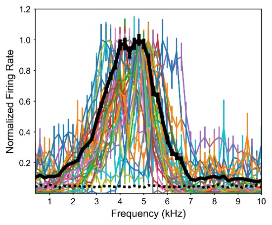
Figure L1. Frequency tuning of frontally-tuned ICx neurons in ruff-removed owls. Tuning curves are normalized by the max response. Thick black line indicates the average tuning curve. Dashed black line indicates basal response.
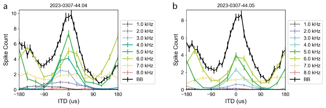
Figure L2. ITD sensitivity across frequencies in ruff-removed owl. Two example neurons shown in a and b. ITD tuning for tones (colored) and broadband (black) plotted by firing rate (non-normalized). Solid colored lines indicate responses to frequencies that are within the neuron’s preferred frequency range (i.e. above the half-height, see Methods), dashed lines indicate frequencies outside of the neuron’s frequency range.
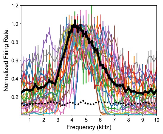
Figure L3. Frequency tuning of frontally-tuned ICx neurons in juvenile owls. Tuning curves are normalized by the max response. Thick black line indicates the average tuning curve. Dashed black line indicates basal response.
3) It would be interesting to have an estimate of the time scale of experience dependency that induces tuning changes. Do the authors have any data on this question? I appreciate the authors' notion that the quantifications in Fig 7 might indicate that juvenile owls are already "beginning to be shaped by ITD reliability" (line 323 in Discussion). How many days after hearing onset would this correspond to? Does this mean that a few days will already induce changes?
While tracking changes induced by ruff-removal over development were outside of the scope of this study, many other studies have assessed experience-dependent plasticity in the barn owl. The recordings in this study were performed approximately 20 days after hearing onset, suggesting that the juveniles had ample time to begin learning. These points were expanded upon in the discussion (Lines 254, 280-283).
Reviewer #2 (Public Review):
1) Why is IPD variability plotted instead of ITD variability (or indeed spatial reliability)? The relationship between these measures is likely to vary across frequency, which makes it difficult to compare ITD variability across frequency when IPDs are plotted. Normalizing data across frequencies also makes it difficult to compare different locations and acoustical conditions. For example, in Fig.1a and Fig.1b, the data shown for 3 kHz at ~160 degrees seems quantitatively and visually quite different, but the difference (in Fig.1c) appears to be negligible.
Justification of why IPD variability is used as an estimate of ITD variability was added to introduction (Lines 55-60), results (Line 100) and methods (Lines 371-374) sections of the manuscript, explaining the fact that because ITD detection is based on phase locking by auditory nerve and ITD detector neurons tuned to narrow frequency bands, responses of ITD detector neurons forwarded to downstream midbrain regions are therefore determined by IPD variability. Additionally, ITD is calculated by dividing IPD by frequency, which makes comparisons of ITD reliability across frequency mathematically uninformative.
2) How well do the measures of ITD reliability used reflect real-world listening? For example, the model used to calculate ITD reliability appears to assume the same (flat) spectral profile for targets and distractors, which are presented simultaneously with the same temporal envelope, and a uniform spatial distribution of sounds across space. It is therefore unclear how robust the study's results are to violations of these assumptions.
While we agree that our analysis cannot completely capture real-world listening for the barn owl, a general analysis using similar flat spectral profiles for targets and concurrent sounds provides a broad assessment of reliability of ITD cues. While a full recapitulation of real-world listening is beyond the scope of this study (i.e. recording natural scenes from the ear canals of wild barn owls), we included additional analyses of ITD reliability in Figure 1-figure supplement 1, described above.
3) Does facial ruff removal produce an isolated effect on ITD variability or does it also produce changes in directional gain, and the relationship between spatial cues and sound location? Although the study considers this issue in some places (e.g. Fig.2, Fig.5), a clearer presentation of the acoustical effects of facial ruff removal and their implications (for all locations, not just those to the front), as well as an attempt to understand how these acoustical changes lead to the observed changes in ITD reliability, would greatly strengthen the study. In addition, Fig.1 shows average ITD reliability across owls, but it would be helpful to know how consistent these measures are across owls, given individual variability in Head-Related Transfer Functions (HRTFs). This potentially has implications for the electrophysiological experiments, if the HRTFs of those animals were not measured. One specific question that is potentially very relevant is whether the facial ruff attenuates sounds presented behind the animal and whether it does so in a frequency-dependent way. In addition, if facial ruff removal enables ILDs to be used for azimuth, then ITDs may also become less necessary at higher frequencies, even if their reliability remains unchanged.
Additional analysis was conducted to generate representation of changes in directional gain induced by ruff removal, added to new figure (Fig 5). This analysis shows that changes in gain following ruff-removal are largely frequency-independent: there is a de-attenuation of peripherally and rearwardly located sounds, but the highest gain remains for high frequencies in frontal space. There is an additional increase in gain for high frequencies from rearward space, these changes would not explain the changes in frequency tuning we report. As mentioned in new additions to the manuscript, the changes at the most rearward-located auditory spatial locations are unlikely to have an effect on the auditory midbrain. No studies in the barn owl have found neurons in the ICx or optic tectum tuned to >120° (Knudsen, 1982; Knudsen, 1984; Cazettes et al., 2014). In addition, variability of IPD reliability across owls was analyzed and reported in the amended Figure 1, which notes very little changes across owls. In this analysis, we did realize that the file of one of the HRTFs obtained from von Campenhausen et al. 2006 was mislabeled, which explains slight differences in revised Fig 1b. Nevertheless, added analysis of IPD reliability across owls indicates that the pattern in ITD reliability is stable across owls (Fig. 1d,e), which supports our decision to not record HRTFs from owls used in this study. Finally, we added to the discussion that clarifies that the use of ILD for azimuth would not provide the same resolution as ITD would (Lines 295-303). We also do not believe that the use of ILD for azimuth would make “ITDs… less necessary at higher frequencies”, given that the ICCls is still computing ITD at these high frequencies (Fig 4), and that ILDs also have higher resolution at higher frequencies, with and without the facial ruff (Olsen et al, 1989; Keller et al., 1998; von Campenhausen et al., 2006).
1) It is unclear why some analyses (Fig.5, Fig.7) are focused on frontal locations and frontally-tuned neurons. It is also unclear why neurons with a best ITDs of 0 are described as frontally tuned since locations behind the animal produce an ITD of 0 also. Related to this, in Fig.1, facial ruff removal appears to reduce IPD variability at low frequencies for locations to the rear (~160 degrees), where the ITD is likely to be close to 0. Neurons with a best ITD of 0 might therefore be expected to adjust their frequency tuning in opposite directions depending on whether they are tuned to frontal or rearward locations.
An extensive explanation was added to the methods detailing why we do not believe the neurons recorded in this study are tuned to the rear. Namely, studies mapping the barn owl’s ICx and optic tectum have not reported neurons tuned to locations >120°, with the number of neurons representing a given spatial location decreasing with eccentricity (Knudsen, 1982; Knudsen, 1984; Cazettes et al., 2014). While we agree that there does seem to be a change in ITD reliability at ~160° following ruff-removal, the result is largely similar to the change that occurs in frontal space (Fig 1b), which is consistent with the ruff-removed head functioning as a sphere. Thus, we wouldn’t expect rearwardly-tuned neurons, if they could be readily found, to adjust their frequency tuning to higher frequencies. Finally, we want to clarify that we focused our analyses on frontally-tuned neurons because frontal space is where we observed the largest change in ITD reliability. Text was added to the Discussion section to clarify this point (Lines 313-321).
2) The study suggests that information about high-frequency ITDs is not passed on to the ICX if the ICX does not contain neurons that have a high best frequency. However, neurons might be sensitive to ITDs at frequencies other than the best frequency, particularly if their frequency tuning is broader. It is also unclear whether the best frequency of a neuron always corresponds to the frequency that provides the most reliable ITD information, which the study implicitly assumes.
The concern about ITD sensitivity at non-preferred frequencies was addressed under the essential revision #3, as well as under Reviewer 1’s concerns.
Author Response
Reviewer #1 (Public Review):
This manuscript provides a comprehensive investigation of the effects of the genetic ablation of three different transcription factors (Srf, Mrtfa, and Mrtfb) in the inner ear hair cells. Based on the published data, the authors hypothesized that these transcription factors may be involved in the regulation of the genes essential for building the actin-rich structures at the apex of hair cells, the mechanosensory stereocilia and their mechanical support - the cuticular plate. Indeed, the authors found that two of these transcription factors (Srf and Mrtfb) are essential for the proper formation and/or maintenance of these structures in the auditory hair cells. Surprisingly, Srf- and Mrtfb- deficient hair cells exhibited somewhat similar abnormalities in the stereocilia and in the cuticular plates even though these transcription factors have very different effects on the hair cell transcriptome. Another interesting finding of this study is that the hair cell abnormalities in Srfdeficient mice could be rescued by AAV-mediated delivery of Cnn2, one of the downstream targets of Srf. However, despite a rather comprehensive assessment of the novel mouse models, the authors do not have yet any experimentally testable mechanistic model of how exactly Srf and Mrtfb contribute to the formation of actin cytoskeleton in the hair cells. The lack of any specific working model linking Srf and/or Mrtfb with stereocilia formation decreases the potential impact of this study.
Major comments:
Figures 1 & 3: The conclusion on abnormalities in the actin meshwork of the cuticular plate was based largely on the comparison of the intensities of phalloidin staining in separate samples from different groups. In general, any comparison of the intensity of fluorescence between different samples is unreliable, no matter how carefully one could try matching sample preparation and imaging conditions. In this case, two other techniques would be more convincing: 1) quantification of the volume of the cuticular plates from fluorescent images; and 2) direct examination of the cuticular plates by transmission electron microscopy (TEM).
In fact, the manuscript provides no single TEM image of the F-actin abnormalities either in the cuticular plate or in the stereocilia, even though these abnormalities seem to be the major focus of the study. Overall, it is still unclear what exactly Srf or Mrtfb deficiencies do with F-actin in the hair cells.
Yes, we agree. As suggested by the reviewer, to directly examine the defects in F-actin organization within the cuticular plate of mutant mice, we conducted Transmission Electron Microscopy (TEM) analyses. The results, as presented in the revised Figures 1 and 4 (panels F, G, and E, F, respectively), provide crucial insights into the structural changes in the cuticular plate. Meanwhile, the comparison of the volume of the phalloidin labeled cuticular plate after 3-D reconstruction using Imaris software was conducted and shown in Author response image 1. The results of the cuticular plate (CP) volume were consistent with the relative F-actin intensity change of the cuticular plate in the revised Figures 1B and 4B. For the TEM analysis of the stereocilia, we regret that due to time constraints, we were unable to collect TEM images of stereocilia with sufficient quality for a meaningful comparison. However, we believe that the data we have presented sufficiently addresses the primary concerns, and we appreciate the reviewers’ understanding of these limitations.
Author response image 1.
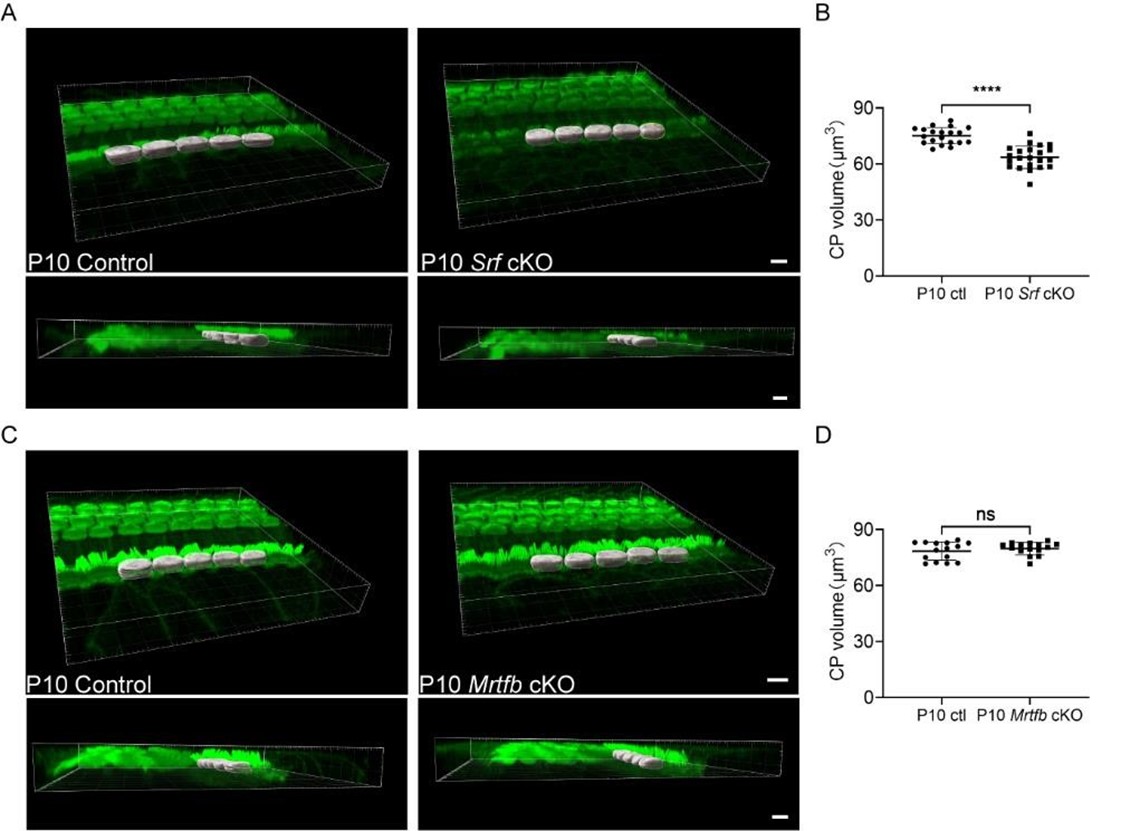
Figures 2 & 4 represent another example of how deceiving could be a simple comparison of the intensity of fluorescence between the genotypes. It is not clear whether the reduced immunofluorescence of the investigated molecules (ESPN1, EPS8, GNAI3, or FSCN2) results from their mis-localization or represents a simple consequence of the fact that a thinner stereocilium would always have a smaller signal of the protein of interest, even though the ratio of this protein to the number of actin filaments remains unchanged. According to my examination of the representative images of these figures, loss of Srf produces mis-localization of the investigated proteins and irregular labeling in different stereocilia of the same bundle, while loss of Mrtfb does not. Obviously, a simple quantification of the intensity of fluorescence conceals these important differences.
Yes, we agree. In addition to the quantification of tip protein intensity, we have added a few more analyses in the revised Figure 3 and Figure 6, such as the percentage of row 1 tip stereocilia with tip protein staining and the percentage of IHCs with tip protein staining on row 2 tip. Using the results mentioned above, the differences in the expression level, the row-specific distribution and the irregular labeling of tip proteins between the control and the mutants can be analyzed more thoroughly.
Reviewer #2 (Public Review):
The analysis of bundle morphology using both confocal and SEM imaging is a strength of the paper and the authors have some nice images, especially with SEM. Still, the main weakness is that it is unclear how significant their findings are in terms of understanding bundle development; the mouse phenotypes are not distinct enough to make it clear that they serve different functions so the reader is left wondering what the main takeaway is.
Based on the reviewer’s comments, in this revised manuscript, we put more emphasis on describing the effects of SRF and MRTFB on key tip proteins’ localization pattern during stereocilia development, represented by ESPN1, EPS8 and GNAI3, as well as the effects of SRF and MRTFB on the F-actin organization of cuticular plate using TEM. We have made substantial efforts to interpret the mechanistic underpinnings of the roles of SRF and MRTFB in hair cells. This is reflected in the revised Figures 1, 3, 4, 6, and 10, where we provide more comprehensive insights into the mechanisms at play.
We interpret our data in a way that both SRF and MRTF regulate the development and maintenance of the hair cell’s actin cytoskeleton in a complementary manner. Deletion of either gene thus results in somewhat similar phenotypes in hair cell morphology, despite the surprising lack of overlap of SRF and MRTFB downstream targets in the hair cell.
In Figure 1 and 3, changes in bundle morphology clearly don't occur until after P5. Widening still occurs to some extent but lengthening does not and instead the stereocilia appear to shrink in length. EPS8 levels appear to be the most reduced of all the tip proteins (Srf mutants) so I wonder if these mutants are just similar to an EPS8 KO if the loss of EPS8 occurred postnatally (P0-P5).
To address this question, we performed EPS8 staining on the control and Srf cKO hair cells at P4 and P10. We found that the dramatic decrease of the row 1 tip signal for EPS8 started since P4 in Srf cKO IHCs. Although the major hair bundle phenotype of Eps8 KO, including the defects of row 1 stereocilia lengthening and additional rows of short stereocilia also appeared in Srf cKO IHCs, there are still some bundle morphology differences between Eps8 KO and Srf cKO. For example, firstly, both Eps8 KO OHCs and IHCs showed additional rows of short stereocilia, but we only observed additional rows of short stereocilia in Srf cKO IHCs. Secondly, in Valeria Zampini’s study, SEM and TEM images did not show an obvious reduction of row 2 stereocilia widening (P18-P35), while our analysis of SEM images confirmed that the width of row 2 IHC stereocilia was drastically reduced by 40% in Srf cKO (P15). Generally, we think although Srf cKO hair bundles are somewhat similar to Eps8 KO, the Srf cKO hair bundle phenotype might be governed by multiple candidate genes cooperatively.
Reference:
Valeria Zampini, et al. Eps8 regulates hair bundle length and functional maturation of mammalian auditory hair cells. PLoS Biol. 2011 Apr;9(4): e1001048.
A major shortcoming is that there are few details on how the image analyses were done. Were SEM images corrected for shrinkage? How was each of the immunocytochemistry quantitation (e.g., cuticular plates for phalloidin and tip staining for antibodies) done? There are multiple ways of doing this but there are few indications in the manuscript.
We apologize for not making the description of the procedure of images analyses clear enough. As described in Nicolas Grillet group’s study, live and mildly-fixed IHC stereocilia have similar dimensions, while SEM preparation results in a hair bundle at a 2:3 scale compared to the live preparation. In our study, the hair cells selected for SEM imaging and measurements were located in the basal turn (30-32kHz), while the hair cells selected for fluorescence-based imaging and measurements were located in the middle turn (20-24kHz) or the basal turn (32-36kHz). Although our SEM imaging and fluorescence-based imaging of basal turn’s hair bundles were not from the same area exactly, the control hair bundles with SEM imaging have reduced row 1 stereocilia length by 10%-20%, compared to the control hair bundles with fluorescence-based imaging (revised Figure 2 and Figure 5). Generally, our stereocilia dimensions data showed appropriate shrinkage caused by the SEM preparation.
Recognizing the need for clarity, we have provided a detailed description of our image quantification and analysis procedures in the “Materials and Methods” section, specifically under “Immunocytochemistry.” This will aid readers in understanding our methodologies and ensure transparency in our approach.
Reference:
Katharine K Miller, et al. Dimensions of a Living Cochlear Hair Bundle. Front Cell Dev Biol. 2021 Nov 25:9:742529.
The tip protein analysis in Figs 2 and 4 is nice but it would be nice for the authors to show the protein staining separately from the phalloidin so you could see how restricted to the tips it is (each in grayscale). This is especially true for the CNN2 labeling in Fig 7 as it does not look particularly tip specific in the x-y panels. It would be especially important to see the antibody staining in the reslices separate from phalloidin.
Thank you for the suggestions. We have shown tip proteins staining in grayscale separately from the phalloidin in the revised Figure 3 and Figure 6. To clearly show the tip-specific localization of CNN2, we conducted CNN2 staining at different ages during hair bundle development and showed CNN2 labeling in grayscale and in reslices in revised Figure 9-figure supplement 1B.
In Fig 6, why was the transcriptome analysis at P2 given that the phenotype in these mice occurs much later? While redoing the transcriptome analysis is probably not an option, an alternative would be to show more examples of EPS8/GNAI/CNN2 staining in the KO, but at younger ages closer to the time of PCR analysis, such as at P5. Pinpointing when the tip protein intensities start to decrease in the KOs would be useful rather than just showing one age (P10).
We agree with the reviewer. To address this question, we have performed ESPN1, EPS8 and GNAI3 staining on the control and the mutant’s hair cells at P4, P10 and P15 (the revised Figures 3 and 6). According to the new results, we found that the dramatic decreases of the row 1 tip signal for ESPN1 and EPS8 started since P4 in Srf cKO IHCs, is consistent with the appearance of the mild reduction of row 1 stereocilia length in P5 Srf cKO IHCs. For Mrtfb cKO hair cells, the obvious reduction of the row 1 tip signal for ESPN1 was observed until P10. However, a few genes related to cell adhesion and regulation of actin cytoskeleton were significantly down-regulated in P2 Mrtfb deficient hair cell transcriptome. We think that in hair cells the MRTFB may not play a major role in the regulation of stereocilia development, so the morphological defects of stereocilia happened much later in the Mrtfb mutant than in the Srf mutant.
While it is certainly interesting if it turns out CNN2 is indeed at tips in this phase, the experiments do not tell us that much about what role CNN2 may be playing. It is notable that in Fig 7E in the control+GFP panel, CNN2 does not appear to be at the tips. Those images are at P11 whereas the images in panel A are at P6 so perhaps CNN2 decreases after the widening phase. An important missing control is the Anc80L65-Cnn2 AAV in a wild-type cochlea.
We agree with the reviewer. We have conducted more immunostaining experiments to confirm the expression pattern of CNN2 during the stereocilia development, from P0 to P11. The results were included in the revised Figure 9-figure supplement 1B. As the reviewer suggested, CNN2 expression pattern in control cochlea injected with Anc80L65-Cnn2 AAV has also been provided in revised Figure 9E.
Author Response
Reviewer #1 (Public Review):
This is an awesome comprehensive manuscript. Authors start by sorting putative stromal cellcontaining BM non-hematopoietic (CD235a-/CD45-) plus additional CD271+/CD235a/CD45- populations to identify nine individual stromal identities by scRNA-seq. The dual sorting strategy is a clever trick as it enriches for rare stromal (progenitor) cell signals but may suffer a certain bias towards CD271+ stromal progenitors. The lack of readable signatures already among CD45-/CD45- sorts might argue against this fear. This reviewer would appreciate a brief discussion on number & phenotype of putative additional MSSC phenotypes in light of the fact that the majority of 'blood lineage(s)'-negative scRNA-seq signatures identified blood cell progenitor identities (glycophorin A-negative & leukocyte common antigen-negative). The nine stromal cell entities share the CXCL12, VCAN, LEPR main signature. Perhaps the authors could speculate if future studies using VCAN or LEPRbased sort strategies could identify additional stromal progenitor identities?
We would like to thank the reviewer for critically evaluating our work and for the generally positive evaluation of the paper. We apologize for delayed resubmission as it took a long time for a specific antibody to arrive to complete the confocal microscopy analyses.
The reviewer asks for a brief discussion on the cell numbers and phenotypes of MSSC phenotypes. The cell numbers and percentages of MSSC in sorted CD45low/-CD235a- and CD45low/-CD235a-CD271+ cells can be found in Supplementary File 3 and we have added a summary of the phenotypes of MSSC in the new Supplementary File 7.
Due to the extremely low frequency of stromal cells in human bone marrow, we chose a sorting strategy that also included CD45low cells (Fig 1A) to ensure that no stromal cells were excluded from the analysis. Although stromal elements are certainly enriched using this approach, the CD45low population contains several different hematopoietic cell types. These include CD34+ HSPCs which are characterized by low CD45 expression2, as well as the CD45low-expressing fractions of other hematopoietic cell populations such as B cells, T cells, NK cells, megakaryocytes, monocytes, dendritic cells, and granulocytes. Furthermore, CD235a- late-stage erythroid progenitors, which are negative for CD45, are represented as well. Of note, our data are consistent with previously reported murine studies showing the presence of a number of hematopoietic populations in CD45- cells, which accounted for the majority of CD45-Ter119-CD31- murine BM cells3,4. However, despite a certain enrichment of stromal elements in the CD45low cell fraction, frequencies were still too low to allow for a detailed analysis of this important bone marrow compartment. This prompted us to adopt the stromal cell-enrichment strategy as described in the manuscript to achieve a better resolution of the stromal compartment. In fact, sorting based on CD45low/-CD235a-CD271+ allowed us to sufficiently enrich bone marrow stromal cells to be clearly detectable in scRNAseq analysis. According to the reviewer’s suggestion, a brief discussion on this issue is now included in the Discussion (page 28, lines 10-15).
The reviewer also suggested using VCAN or LEPR-based sorting strategy to identify additional stromal identities in future studies.
However, as an extracellular matrix protein, FACS analysis of cellular VCAN expression can only be achieved based on its intracellular expression after fixation and permeabilization5,6. Additionally, while VCAN is highly and ubiquitously expressed by stromal clusters, VCAN is also expressed by monocytes (cluster 36). Therefore, VCAN is not an optimal marker to isolate viable stromal cells.
LEPR is the marker that was reported to identify the majority of colony-forming cells in adult murine bone marrow7. We have previously reported that the majority of human adult bone marrow CFU-Fs is contained in the LEPR+ fraction 8. In our current scRNAseq surface marker profiling analysis, group A cells showed high expression of several canonical stromal markers including VCAM1, PDGFRB, ENG (CD73), as well as LEPR (Fig. 4A). However, the four stromal clusters in Group A could not be separated based on the expression of LEPR. Therefore, we chose not to use LEPR as a marker to prospectively isolate the different stromal cell types.
The authors furthermore localized CD271+, CD81+ and NCAM/CD56+ cells in BM sections in situ. Finally, referring to the strong background of the group in HSC research, in silico prediction by CellPhoneDB identified a wide range of interactions between stromal cells and hematopoietic cells. Evidence for functional interdependence of FCU-F forming cells is completing the novel and more clear bone marrow stromal cell picture.
We thank the reviewer for the positive comments.
An illustrative abstract naming the top9 stromal identities in their top4 clusters by their "top10 markers" + functions would be highly appreciated.
We thank the reviewer for the suggestion. A summary of the characteristics of stromal clusters is now shown in the new Supplementary File 7, which we hope matches the reviewer’s expectations.
Reviewer #2 (Public Review):
Knowledge about composition and function of the different subpopulations of the hematopoietic niche of the BM is limited. Although such knowledge about the mouse BM has been accumulating in recent years, a thorough study of the human BM still needs to be performed. The present manuscript of Li and coworkers fills this gap by performing single cell RNA sequencing (scRNAseq) on control BM as well as CD271+ BM cells enriched for non-hematopoietic niche cells.
We apologize for delayed resubmission as it took a long time for a specific antibody to arrive to complete the confocal microscopy analyses. We thank the reviewer for the critical expert review and overall positive comments.
Based on their scRNAseq, the authors propose 41 different BM cell populations, ten of which represented non-hematopoietic cells, including one endothelial cell cluster. The nine remaining skeletal subpopulations were subdivided into multipotent stromal stem cells (MSSC), four distinct populations of osteoprogenitors, one cluster of osteoblasts and three clusters of pre-fibroblasts. Using bioinformatic tools, the authors then compare their results and divisions of subpopulations to some previously published work from others and attempt to delineate lineage relationships using RNA velocity analyses. From these, they propose different paths from which MSSC enter the progenitor stages, and might differentiate into pre-osteoblasts and -fibroblasts.
It is of interest to note, that apparently adipo-primed cells may also differentiate into osteolineage cells, something that should be further explored or validated. Furthermore, although this analysis yields a large adipo-primed populations, pre-adipocytes and mature adipocytes appear not to be included in the data set the authors used, which should also be explained.
We thank the reviewer for this comment. We chose to annotate Cluster 5 as adipoprimed cluster based on the higher expression of adipogenic differentiation markers as well as a group of stress-related transcription factors (FOS, FOSB, JUNB, EGR1) (Fig. 2B-C, Figure 2-figure supplement 1C) some of which had been shown to mark bone marrow adipogenic progenitors1. Although at considerably lower levels compared to adipogenic genes, osteogenic genes were also expressed in cluster 5 cells (Fig. 2B and D), indicating the multi-potent potential of this cluster. Therefore, our initial annotation of these cells as adipoprimed progenitors was too narrow as it did not include the possible osteogenic differentiation potential. We apologize for the confusion caused by the inappropriate annotation and, in order to avoid any further confusion, cluster 5 has now been re-annotated as ‘highly adipocytic gene-expressing progenitors (HAGEPs), which we believe is a better representation of the cells. We furthermore agree with the reviewer that in-vivo differentiation needs to be performed to address potential differentiation capacities in future studies.
With regard to the lack of adipocytes in our data set, we described in the Materials and Methods section that human bone marrow cells were isolated based on density gradient centrifugation. After centrifugation, the mononuclear cell-containing monolayers were harvested for further analysis. However, the resulting supernatant containing mature adipocytic cells was discarded14. Therefore, adipocyte clusters were not identified in our dataset. We have amended the manuscript accordingly (page 5, line 7).
Regarding the pre-adipocytes, we are not aware of any specific markers for pre-adipocytes in the bone marrow. We examined the only known markers (ICAM1, PPARG, FABP4) that have been shown to mark committed pre-adipocytes in human adipose tissue15. As illustrated in Fig. R1 (below), low expression of all three markers was not restricted to a single distinct cluster but could be found in almost all stromal clusters. These data thus allow us to neither confirm nor exclude the presence of pre-adipocytes in the dataset. Due to the lack of specific markers for pre-adipocytes and the absence of mature adipocytes in the current dataset, it is therefore difficult to identify a well-defined pre-adipocytes cluster.
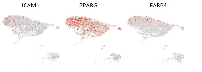
Figure R1. UMAP illustration of the normalized expression of the markers for pre-adipocytes in stromal clusters.
In addition, based on a separate analysis of surface molecules, the authors propose new markers that could be used to prospectively isolate different human subpopulations of BM niche cells by using CD52, CD81 and NCAM1 (=CD56). Indeed, these analyses yield six different populations with differential abilities to form fibroblast-like colonies and differentiate into adipo-, osteo-, and chondrogenic lineages. To explore how the scRNAseq data may help to understand regulatory processes within the BM, the authors predict possible interactions between hematopoietic and non-hematopoietic subpopulations in the BM. These should be further validated, to support statements as the suggestion in the abstract that separate CXCL12- and SPP1-regulated BM niches might exist.
We agree with the reviewer that functional validation of the CellPhoneDB results using for example in vivo humanized mouse models would be needed to demonstrate the presence of different niches in the bone marrow. At this point of time we only put forward the hypothesis that different niche types exist while we will work on providing experimental proof in our future studies.
The scRNAseq analysis is indeed a strong and important resource, also for later studies meant to increase knowledge about the hematopoietic niche of the BM. Although the analyses using different bioinformatic tools is very helpful, they remain mostly speculative, since validatory experiments, as already mentioned, are missing. As such, I feel the authors did not succeed in achieving their goals of understanding how non-hematopoietic cells of the BM regulate the different hematopoietic processes within the BM. Nevertheless, they have created valuable resources, both in the scRNAseq data they generated, as well as the different predictions about different cell populations, their lineage relationships, and how they might interact with hematopoietic cells.
We thank the reviewer for the appreciation of the value of this dataset. We agree with the reviewer that it is of great importance to validate the contribution of potential driver genes for stromal cell differentiation and verify the in vitro data and in-silico prediction using in-vivo models. As the main goal of the current study was to formulate hypotheses based on the scRNAseq data for future studies, we believe that in vivo validation experiments using engineered human bone marrow models or humanized bone marrow ossicles are out of the scope of the current study, but certainly need to be performed in the future.
The impact of this work is difficult to envision, since validations still need to be performed. Also, it has the born in mind that humans are not mice, which can be studied in neat homogeneous inbred populations. Human populations on the other hand, are quite diverse, so that the data generated in this manuscript and others will probably have to be combined to extrapolate data relevant to the whole of the human population. However, as it is equally difficult to generate reliable scRNAseq data from human BM, it seems likely that the data will indeed an important resource, when more data from different donors become available.
We thank the reviewer for the generally positive evaluation of this study.
Taken at point value, the authors provide evidence that human counterparts exist to several BM populations described in mice. In my opinion, the lineage relationships predicted using the RNA velocity analyses need more substance, as it seems the differentiation-paths may diverge from what is known from mice. If so, this issue should be studied more stringently. Similarly, the paper would have been strengthened considerably if a relevant experimental validation would have been attempted, perhaps by using genetically modified (knockdown) MSSC, similar to Battula et al. (doi: 10.1182/blood-2012-06-437988).
In the study from Welner’s group, stromal differentiation trajectory was inferred based on scRNAseq analysis of murine bone marrow cells using Velocyto16. Velocyto identified MSCs as the ‘source’ cell state with pre-adipocytes, pro-osteoblasts, and prochondrocytes being end states. In our study, the MSSC population was predicted to be at the apex of the trajectory and the pre-osteoblast cluster was placed close to the terminal state of differentiation, which is consistent with the murine study. However, different stromal cell types were identified in mice compared with humans. For example, we have identified prefibroblasts in our dataset which are absent in the murine study, while a well-defined murine pre-adipocyte population was not identified in our human dataset. Therefore, it is not surprising to find some discrepancies between human and murine stromal differentiation trajectories. Of course and as mentioned before, critical in-vivo functional validations need to be carried out to address these important issues in the future.
In summary, this is a very interesting but also descriptive paper with highly important resources. However, to prospectively identify or isolate human non-hematopoietic/nonendothelial niche populations, more stringent validations should have been performed to strengthen the validity of the different analyses that have been performed. As such, it remains an open question which niche subpopulations has the most impact on the different hematopoietic processes important for normal and stress hematopoiesis, as well as malignancies.
Thank you for this comment. We completely agree that more stringent validations are necessary but are outside of the aim of our current hypothesis-generating study. Accordingly, we are planning functional verification studies using genetically manipulated stromal cells in combination with in-vivo humanized ossicles. Furthermore, other groups will hopefully use our database and contribute with functional studies in model systems that are currently not available to us, e.g. iPS-derived bone marrow in-vitro proxies.
Specific remarks
• Since CD45, CD235a, and CD271 are used as distinguishing markers in the sample preparation of the scRNAseq, it would be helpful to highlight these markers in the different analyses (Figures 1D, 2B, 2C-F, and 4A), and restrict the analyses to those cells that also not express CD45, CD235a (why use CD71?) and highly express CD271.
Thank you for this comment. As shown in Fig. R2, we have modified figures Fig. 1D, 2B, and 4A showing now also the expression of PTPRC (CD45), GYPA (CD235a), and NGFR (CD271) on the top (Fig. 1D and 2B) or right (Fig. 4A) panel of the figures. To complement Fig. 2C-F, we have generated new stacked violin plots showing the expression level of three markers by all 9 stromal clusters (Fig. R2B). As we believe that including these three markers in the figures does not provide a better strategy to improve the analyses, we decided to leave the original figures unchanged in this respect.
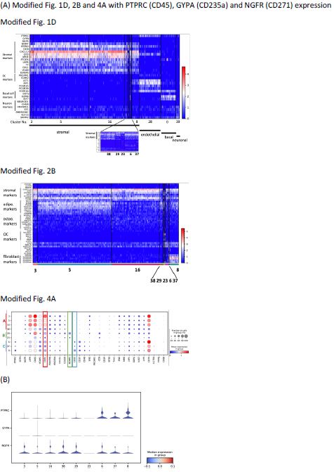
Figure R2. (A) Modified Fig. 1D, 2B and 4A with PTPRC (CD45), GYPA (CD235a) and NGFR (CD271) expression. (B) Stacked violin plots of PTPRC, GYPA and NGFR expressed by stromal clusters to complement Fig. 2C-F.
With regard to cell exclusion based on CD45, as shown in the modified Figure corresponding to Fig 1A in the manuscript (Fig R2A), CD45 gene expression is observed also in the endothelial cluster, basal cluster, and neuronal cluster (Fig. R2A). These clusters represent non-hematopoietic clusters that we would like to keep in our dataset for further analysis, such as cell-cell interaction. Therefore, we choose to not restrict the analysis to solely CD45 nonexpressing cells.
With regard to CD235a (GYPA), expression of CD235a is not detected in any of the nonhematopoietic clusters. Thus, CD235a-expressing cell exclusion is not necessary.
For CD271, according to our previous results (own unpublished data, belonging to a dataset of which only significantly expressed genes were reported in Li et al.8), protein expression of CD271 is not necessarily reflected by gene expression. In the other words, stromal cells with CD271 protein expression do not always have high mRNA expression. A significant fraction of stromal cells would be excluded if we restrict the analyses only to those cells that show high CD271 gene expression, which would not reflect the real cellular composition of human bone marrow stroma. In order to not risk losing stromal cells, we therefore kept our previous analyses which included stromal cells with various CD271 expression levels.
With regard to using CD71 as an exclusion marker, please see also the comments to reviewer 1. Briefly, according to our data, CD71 (TFRC)-expressing erythroid precursors could still be found after excluding CD45 and CD235a positive cells (Figure 1-figure supplement 1B and R3). As furthermore shown in Figure 1-figure supplement 1G and R2, CD71 expression in the stromal clusters is negligible. Therefore, we believe that this justifies the use of CD71 as an additional marker to exclude erythroid cells. We have amended the discussion to address this issue (page 19, lines 7-8).
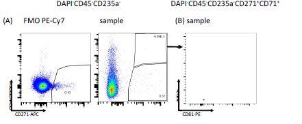
Figure R3. FACS plots illustrating the expression of (A) CD71 (TFRC) vs CD271 in CD45- CD235a- cells and (B) FSC-A vs CD81 in CD45-CD235a-CD271+CD71+ cells following exclusion of doublets and dead cells.
• Despite a distinct neuronal cluster (39), there does not seem to be a distinctive marker for these cells. Is this true?
Yes, the reviewer is correct that there is no significantly-expressed distinctive marker for neuronal cells. Multiple markers indicating the presence of different cell types were identified in cluster 39 (Supplementary File 4). Among them, several neuronal markers (NEUROD1, CHGB, ELAVL2, ELAVL3, ELAVL4, STMN2, INSM1, ZIC2, NNAT) were found to be enriched in this cluster (Supplementary File 4 and Fig. 1D) with higher fold changes compared to other identified genes. However, the expression of these genes was not statistically significant, which is mainly due to the heterogeneity of the cluster and thus does not allow us to draw any firm conclusions.
Several genes including MALAT1, HNRNPH1, AC010970.1, and AD000090.1 were identified to be statistically highly expressed by cluster 39 (Supplementary File 4). The expression of these genes is not restricted to any specific cell type. It is therefore impossible to annotate the cluster based on this and our data thus indicated that cluster 39 is a heterogeneous population containing multiple cell types. Based on the expression of neuronal markers, we nevertheless chose to annotate Cluster 39 as “neuronal” as the prominent expression of neuronal markers indicated the presence of neurons in this cluster. To be more accurate, the annotation of cluster 39 has been changed to ‘neuronal cell-containing cluster’ to correctly reflect the presence of non-neuronal gene expressing cells as well (page 29, lines 3-8).
• Since based on 2C and 2D, the authors are unable to distinguish adipo- from osteogenic cells, would the authors use the same molecules to distinguish different populations of 2C-D, or would they use other markers, if so which and why.
We agree with the reviewer that at the first glance adipo-primed (cluster 5, now annotated as “highly adipocytic gene-expressing progenitors”, HAGEPs), balanced progenitors (cluster 16), and pre-osteoblasts (cluster 38) shared a similar expression pattern according to the violin plots in Fig. 2C and 2D. However, as illustrated in the heatmap (Fig. 2B), the expression patterns of adipo-primed (HAGEP) and balanced progenitors were quite different in terms of their expression of adipogenic and osteogenic markers. Both adipogenic and osteogenic marker expression was detected in HAGEPs, balanced progenitors, and preosteoblasts. Thus, as violin plots are summarizing the overall expression levels of a certain marker in a certain cluster, these plots tend to make it more difficult to detect differential expression patterns between different clusters. In this case, the heatmap shown in Fig. 2B is a good complement to the violin plots as it is demonstrating the different expression patterns of every cell in the different stromal clusters.
Additionally, cluster 5 showed the expression of a group of stress-related transcription factors (FOS, FOSB, JUNB, EGR1) (Fig. 2B and Figure 2-figure supplement 1C), some of which had been shown to mark bone marrow adipogenic progenitors1. The expression of the abovementioned stress-related transcription factors (putative adipogenic progenitor markers) was generally lower in cluster 38 compared to cluster 5, further demonstrating that clusters were different.
Furthermore, there was a gradual upregulation of more mature osteogenic markers such as RUNX1, CDH11, EBF1, and EBF3 from cluster 5 to cluster 16 and finally cluster 38. As shown in Fig. 2D, the expression of these markers was higher in cluster 38 compared to cluster 5. Therefore, cluster 38 was annotated as pre-osteoblasts.
Most of the stromal clusters form a continuum (Fig. 2A), which correlates very well with the gradual transition of different cellular states during stromal cell development. It is highly unlikely that abrupt and dramatic gene expression changes would occur during the cellular state transition of cells of the same lineage. Therefore, it is not surprising to find the differences in gene expression profiles between stromal clusters share a certain level of similarities.
In summary, we rely on several factors to distinguish different stromal clusters, which include canonical adipo-, osteo- and chondrogenic markers, stress markers, heatmap, violin plots, and the gradual up-regulation of certain lineage-specific markers.
To directly answer the reviewer’s question, we believe that we are able to distinguish different stromal clusters based on our data.
• In de Jong et al., an inflammatory MSC population (iMSC) is defined. Since the Schneider group showed that inflammatory S100A8 and A9 are expressed by inflamed MSC, is it possible that the some of the designated pre-fibroblasts actually correspond to these S100A8/A9-expressing iMSC?
We thank the reviewer for raising this interesting question.
First of all, we would like to point out that scRNAseq was performed using viably frozen bone marrow aspirates in de Jong’s study while freshly isolated bone marrows were used in our study. There might be discrepancies between frozen and fresh bone marrow samples in terms of cellular composition including stromal composition and, importantly, processinginduced stress-related gene expression profiles.
To investigate if designated pre-fibroblasts actually correspond to iMSCs as suggested by the reviewer, we have re-examined the expression of some of the key iMSC genes as reported by de Jong et al 17. As shown in Fig. R6, the markers that can distinguish iMSC from other MSC clusters in de Jong et al. study were not exclusively expressed by pre-fibroblasts, but also by other stromal cell types including HAGEPs, balanced progenitors, and pre-osteoblasts.
In the study by R. Schneider’s group18, significant upregulation of S100A8/S100A9 was observed in stromal cells from patients with myelofibrosis. Furthermore, base-line expression of S100A8/A9 was also observed in the fibroblast clusters in the control group, which correlates very well with our data of S100A8/9 expression in pre-fibroblasts in normal donors (Fig. 2F). Our data thus indicate – in line with Schneider’s findings - that there is a baseline level expression of S100A8/9 in fibroblasts in hematologically normal samples and that the expression of S100A8/9 is not restricted to inflamed MSC.
In summary, the gene expression profiles observed in our study do not indicate the presence of iMSC in the healthy bone marrow.
• Figure 3A: Do human adipo-primed cells (cluster 5) indeed differentiate into osteogenic cells (clusters 6, 38, and 39). This would be highly unexpected. Can the authors substantiate this "reliable outcome of the RNA velocity analysis"?
Please refer to our previous responses regarding this topic. Briefly, as shown in Fig. 2B and D, both osteogenic and adipogenic genes are expressed in cluster 5, indicating the multi-potent potentials of this cluster. Although the cluster was initially annotated as adipo-primed progenitors, this was not intended to exclude the osteogenic differentiation potential of these progenitors. Nevertheless, this annotation did not correctly reflect the differentiation potential and might thus have caused confusion, for which we apologize. In order to more correctly describe the characteristics of these cells, cluster 5 has now been reannotated as ‘highly adipocytic gene-expressing progenitors (HAGEPs)’.
In general, the outcome of the RNA velocity analysis needs to be corroborated by in-vivo differentiation experiments. But we believe that functional verification, which would be extensive, is out of the scope of the current study and we will address these questions in future studies.
• How statistically certain are the authors, that the populations in Figure 4B as defined by flow cytometry, correspond to MSSC, adipo-primed cells, osteoprogenitors, etc., as defined by scRNAseq?
To address this question, we sorted the A1-A4 populations and performed RT- PCR to examine the CD81 expression level in each cluster. As shown in Figure 4-figure supplement 1B, CD81 expression levels were higher in A1 and A2 compared with A3 and A4, which is consistent with the scRNAseq data that showed the highest CD81 expression in MSSCs compared to other clusters (Supplementary File 4).
The phenotypes defined in this study allowed us to isolate different stromal cell types which demonstrated significant functional differences as described in the manuscript (page 19, lines 17-25; page 20, lines 1-11). These results, in combination with the quantitative real-time PCR results (Figure 4-figure supplement 1B), demonstrated that the A1-A4 subsets in FACS are functionally distinct populations and are likely to be – at least in large parts – identical or equivalent to the transcriptionally identified clusters in group A stromal cells. However, at this point, we do not have performed the required experiments (scRNAseq of sorted cells) that would provide sufficient proof to confirm this statement statistically.
• The immunohistochemistry results shown do not allow distinct conclusions as the colors give unequivocal mix-colors, and surface expression cannot be distinguished from intracellular expression. Please use a 3D (confocal) method for such statements.
We thank the reviewer for the suggestion and we have performed additional confocal microscopy analysis of human bone marrow biopsies as suggested by the reviewer. Representative confocal images are now presented in the middle and right panel of Fig. 6E. We also include a separate file (Supplemental confocal image file). Here, confocal scans of all maker combinations are shown as ortho views in addition to detailed intensity profile analyses of the cells of interest clearly distinguishing surface staining from intracellular staining.
Confocal analysis of bone marrow biopsies confirmed our findings presented in the manuscript. As observed in the scanning images, CD271-expressing cells were negative for CD45 and were located in perivascular, endosteal, and peri-adipocytic regions. CD271/CD81double positive cells could be found either in the peri-adipocytic regions or perivascular regions while CD271/NCAM1 double-positive cells were exclusively situated at the bone-lining endosteal regions. The results of the confocal analysis have been added to the revised manuscript (page 21, lines 15-17).
• Figure 5A: as all cells seem to interact with all other cells, this figure does not convey relevant information about BM regions using for instance CXCL12 or SPP1. Please reanalyze to show specificity of the interactions of the single clusters. Also, since it is unlikely the CellPhoneDB2-predicted interactions are restricted to hematopoietic responders, please also describe the possible interactions between non-hematopoietic cells.
Fig. 5A was used to demonstrate the complexity of the interactions between hematopoietic cells and stromal cells.
To gain a more detailed understanding of the interactions, we also performed an analysis with the top-listed ligand-receptor pairs as shown in Fig. 5B-C and Figure 5-figure supplement 1B. Here, each dot represents the interaction of a specific ligand-receptor pair listed on the x-axis between the two individual clusters indicated in the y-axis, which we believe shows what the reviewer is asking for.
The specificity of the interactions between single clusters were shown in Fig. 5B-C and Figure 5-figure supplement 1B. The CXCL12- and SPP1-mediated interactions between MSSC/OC and hematopoietic clusters clearly suggested stromal cell type-specific interactions.
Regarding non-hematopoietic cells, both inter- and intra-stromal interactions were identified to be operative between different stromal subsets as well as within the same stromal cell population as shown in Figure 5-figure supplement 3B. In addition, we have also analyzed the interaction pattern between endothelial cells and hematopoietic cells as shown in Fig. 7A, and thus we believe that we have sufficiently described these interactions as requested by the reviewer.
Author Response
Reviewer #2 (Public Review):
Point 1: The transcriptomic analysis of E12.5 endocardial cushion cells in the various mouse models is informative in the extraction of Igf2- and H19-specific gene functions. In Fig. 6D, a huge sex effect is obvious with many more DEGs in female embryos compared to males. How can this be explained given that Igf2/H19 reside on Chr7 and do not primarily affect gene expression on the X chromosome? Is any chromosomal bias observed in the genomic distribution of DEGs?
We examined chromosomal distribution of DEGs between WT and +/hIC1 (Supplemental Figure 6D) and did not see any bias on X chromosome. We described this result on lines 278-280: “Although the number of +/hIC1-specific DEGs largely differed between males and females, there was no sex-specific bias on the X chromosome (Supplemental Figure 6D).” Additionally, we agree with the reviewer that it is noteworthy that the dysregulated H19/Igf2 expression affected transcriptome in a sex-specific manner, especially when the mutation is located on a somatic chromosome. Although investigating the role of hormones versus sex chromosome in these effects would be quite interesting, it is beyond the scope of current study.
Point 2: A separate issue is raised by Fig. 6E that shows a most dramatic dysregulation of a single gene in the delta3.8/hIC1 "rescue" model. Interestingly, this gene is Shh. Hence, these embryos should exhibit some dramatic skeletal abnormalities or other defects linked to sonic hedgehog function.
The reason why Shh appeared to be differentially expressed between wild-type and d3.8/hIC1 samples was that Shh expression was 0 across all the samples except for two wild-type samples. In order to detect all the DEGs that might be lowly expressed, we did not want to filter DEGs based on the level of total expression. As a result, Shh was represented as significantly differently expressed in d3.8/hIC1 samples, although its expression in our samples appears to be too low to have any significant effect on development. This explanation was added to lines 310-312. To confirm that this was an exceptional case, we analyzed the expression of DEGs obtained from other pairwise comparisons. In the volcano plots below, genes of which expression is not statistically different between two groups are marked grey. Genes of which expression is statistically different and detected in both groups are marked red. Genes with statistically different but not detected in one group at all, such as Shh, are marked blue (Figure G). It is clear that that almost all of our DEGs are expressed consistently across the groups, and genes with no expression detected in one group are very rare.
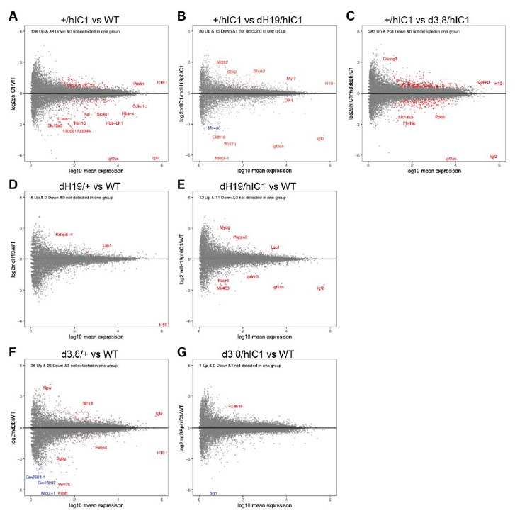
Point 3: The placental analysis needs to be strengthened. Placentas should be consistently positioned with the decidua facing up, and the chorionic plate down. The placentas in Fig. 3F are sectioned at an angle and the chorionic plate is missing. These images must be replaced with better histological sections.
As requested, we have replaced placental images with better representative sections (Figure 3F and 4E). In addition, we have improved alignment of placental histology figures.
Point 4: The CD34 staining has not worked and does not show any fetal vasculature, in particular not in the WT sample.
As requested, we have replaced the CD34 vascular stained images with those that better represent fetal vasculature (Figure 3G).
Point 5: The "thrombi" highlighted in Fig. 4E are well within the normal range, to make the point that these are persistent abnormalities more thorough measurements would need to be performed (number, size, etc).
As requested, we measured the number and relative size of the thrombi that are found in dH19/hIC1 placentas with lesions. No thrombi were found in wild-type placentas whereas an average of 1.3 thrombi were found in six dH19/hIC1 placentas. The size of the thrombi widely varied, but occupied average of 2.58% of the labyrinth zone where these lesions were found (Supplemental Figure 4D). Additionally, we replaced the image in Figure 4E into the section that better represents the lesion.
Point 6: The statement that H19 is disproportionately contributing to the labyrinth phenotype (lines 154/155) is not warranted as Igf2 expression is reduced to virtually nothing in these mice. Even though there is more H19 in the labyrinth than in the junctional zone, the phenotype may still be driven by a loss of Igf2. Given the quasi Igf2-null situation in +/hIC1 mice, is the glycogen cell type phenotype recapitulated in these mice, and how do glycogen numbers compare in the other mouse models?
The sentence was edited in line 157. We performed Periodic acid Schiff (PAS) staining on +/hIC1 placentas to address if glycogen cells are affected by abnormal H19/Igf2 expression (Supplemental Figure 1E). In contrary to previous reports where Igf2-null mice had lower placental glycogen concentration (Lopez et al., 1996) and H19 deletion led to increased placental glycogen storage (Esquiliano et al., 2009), our quantification on PAS-stained images showed that the glycogen content is not significantly different between wild-type and +/hIC1 placentas. We have described this result in lines 166-168.
Point 7: How do delta3.8/+ and delta3.8/hIC1 mice with a VSD survive? Is it resolved some time after birth such that heart function is compatible with postnatal viability? And more importantly, do H19 expression levels correlate with phenotype severity on an individual basis?
Our study was limited to phenotypes prior to birth, thus postnatal/adult phenotypes were not examined. Because the VSD showed only partial penetrance in these mice, we cannot state that the d3.8/+ or d3.8/hlC1 mice with VSDs survive. It has also been previously reported in another mouse model with incomplete penetrance of a VSD that the mice which survived to adulthood did not have the VSDs (Sakata et al., 2002). We find it highly unlikely that either mouse model would survive significantly past the postnatal timepoint with a VSD. We have examined two PN0 d3.8/hIC1 neonates, and both did not have VSD.
Regarding the second point, the only way to quantitatively address this question would be to do qPCR or RNA-seq on individual hearts, which then makes it impossible for those hearts to be examined for histology to confirm the VSD. Thus, hearts used to identify VSDs via histology could not also be used for quantitative H19 measurements. One thing to note is that the H19/Igf2 expression in independent replicates of d3.8/hIC1 cardiac ECs used in our RNA-seq experiment is quite variable, not clustering together in contrast to other mouse models used in this study (Fig. 6A). Such wide range of variability in the extent of H19/Igf2 dysregulation suggests that H19/Igf2 levels could have an impact on the penetrance or the severity of the VSD phenotype in d3.8/hIC1 embryos.
Author Response
Reviewer #2 (Public Review):
Weaknesses:
1) The relevance of the LPS-induced calvarial osteolysis model is not clear. Calvaria is mostly composed of cortical bone-like structures lacking marrow space, though small marrow space exists near the suture. Osteolysis appears to occur in areas apart from where marrow is located. The authors did not show in the manuscript which cells Adipoq-Cre marks in the calvaria.
We have shown in a recent publication that MALPs exist in the calvarial bone marrow (2). As shown in Fig. R1A, Td+ cells are layer of cortical bone (Fig. R1B, blue arrows). In WT mice, after LPS injection, the normal bone structure, including suture and cortical bone, were mostly eroded, and filled with inflammatory cells (green arrows). Thus, osteolysis does occur at the area where bone marrow is originally located. On the contrary, calvarial bone structure was preserved in the CKO mice, demonstrating that Csf1 deficiency in MALPs suppresses LPS-induced osteolysis. We included the H&E staining data in the revised manuscript:
"H&E staining showed that calvarial bone marrow is surrounded by a thin layer of cortical bone (Fig. 5C). After the LPS injection, normal calvarial structure, including suture and cortical bone, were mostly eroded and filled with inflammatory cells in WT mice, but unaltered in CKO mice."
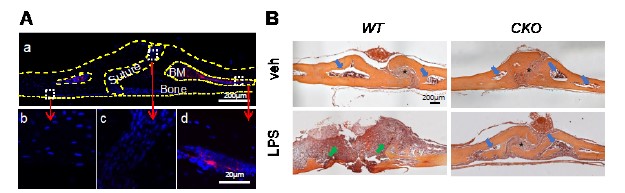
Figure R1. Calvarial bone marrow structure. (A) Representative coronal section of 1.5-month-old Adipoq/Td mouse calvaria. Bone surfaces are outlined by dashed lines. Boxed areas in the low magnification image (top) are enlarged to show periosteum (bottom left), suture (bottom middle), and bone marrow (BM, bottom right) regions. Red: Td; Blue: DAPI. Adopted from our previous publication (2). (B) H&E staining of coronal sections of WT and Csf1 CKOAdipoq mice after LPS injection. Blue arrows point to bone marrow space close to suture (indicated by *). Green arrows point to the osteolytic lesion where cortical bone was eroded, and the space were filled with inflammatory cells.
2) Although the contrast between the two Csf1 conditional deletion models (Adipoq-Cre and Prx1-Cre) is very interesting, the relationship between these two cell populations are not well described. The authors did not clarify if MALPs are also targeted by Prx1-Cre, or these two cell types are from different cell lineages. "Other mesenchymal lineage cells" in the subtitle is not extremely helpful to place this finding in context.
We thank the Reviewer for this comment. The original article constructing Prx1-Cre mouse line demonstrates that Prx1-Cre targets all mesenchymal cells in the limb bud at early as 10.5 dpc (10). This early expression pattern ensures that all bone marrow mesenchymal lineage cells, including MALPs, are targeted by Prx1-Cre. In addition, based on our scRNA-seq data (1), Adipoq is mainly expressed in MALPs, while Prrx1 (Prx1) is highly expressed not only in MALPs but also in EMPs, IMPs, LMPs, LCPs, and OBs (Fig. R2). Thus, the fact that Prx1-Cre driven CKO mice have much more severer bone phenotypes than AdipoqCre driven CKO mice indicates that mesenchymal lineage cells other than MALPs also contribute Csf1 to regulate bone resorption. To avoid confusion, we changed the title and the first sentence in the Result session about Prx1 mice to the following:
"Csf1 from mesenchymal lineage cells other than MALPs regulate bone structure.
To explore whether Csf1 from MALPs plays a dominant role in regulating bone structure, we generated Prx1-Cre Csf1flox/flox (Csf1 CKOPrx1) mice to knockout Csf1 in all mesenchymal lineage cells in bone (10), including MALPs."
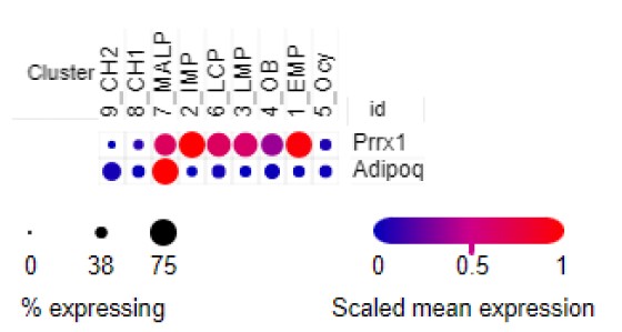
Figure R2. Dotplot of Prrx1 and Adipoq expression in bone marrow mesenchymal lineage cells based on our scRNA-seq analysis of 1-month-old mice.
3) The data supporting defective bone marrow hematopoiesis in Csf1 CKO mice are not particularly strong. They observed a reduction in bone marrow cellularity, but this was only associated with an expected reduction in macrophages and a mild reduction in overall HSPC populations. More in-depth analyses might be required to define mechanisms underlying reduced bone marrow cellularity in CKO mice.
We thank the Reviewer for this constructive comment. Accordingly, we performed a thorough analysis of bone marrow hematopoietic compartments and observed significant decreases of monocytes and erythroid progenitors in CKO mice compared to WT mice. These results are now included as Fig. 6E.
4) Some of the phenotypic analyses are still incomplete. The authors did not report whether CHet (Adipoq-Cre Csf1(flox/+)) showed any bone phenotype. Further, the authors did not report whether Csf1 mRNA or M-Csf protein is indeed expressed by MALPs, with current evidence solely reliant on scRNAseq and qPCR data of bulk-isolated cells. More specific histological methods will be helpful to support the premise of the study.
A pilot microCT study revealed the same femoral trabecular bone structure in WT and Adipoq-Cre Csf1flox/+ (Csf1 Het) mice at 3 months of age (Fig. R3). While the sample number for Het is low, we are confident about this conclusion.
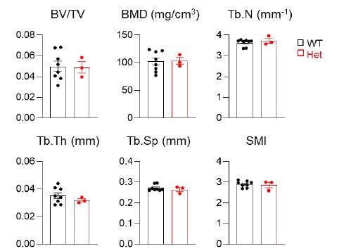
Figure R3. MicroCT measurement of trabecular bone structural parameters from WT and Csf1 Het mice. BV/TV: bone volume fraction; BMD: bone mineral density; Tb.N: trabecular number; Tb.Th: trabecular thickness; Tb.Sp: trabecular separation; SMI: structural model index. n=3-8 mice/group.
Author response:
Reviewer #1 (Public Review):
In this paper, Tompary & Davachi present work looking at how memories become integrated over time in the brain, and relating those mechanisms to responses on a priming task as a behavioral measure of memory linkage. They find that remotely but not recently formed memories are behaviorally linked and that this is associated with a change in the neural representation in mPFC. They also find that the same behavioral outcomes are associated with the increased coupling of the posterior hippocampus with category-sensitive parts of the neocortex (LOC) during a post-learning rest period-again only for remotely learned information. There was also correspondence in rest connectivity (posterior hippocampus-LOC) and representational change (mPFC) such that for remote memories specifically, the initial post-learning connectivity enhancement during rest related to longer-term mPFC representational change.
This work has many strengths. The topic of this paper is very interesting, and the data provide a really nice package in terms of providing a mechanistic account of how memories become integrated over a delay. The paper is also exceptionally well-written and a pleasure to read. There are two studies, including one large behavioral study, and the findings replicate in the smaller fMRI sample. I do however have two fairly substantive concerns about the analytic approach, where more data will be required before we can know whether the interpretations are an appropriate reflection of the findings. These and other concerns are described below.
Thank you for the positive comments! We are proud of this work, and we feel that the paper is greatly strengthened by the revisions we made in response to your feedback. Please see below for specific changes that we’ve made.
1) One major concern relates to the lack of a pre-encoding baseline scan prior to recent learning.
a) First, I think it would be helpful if the authors could clarify why there was no pre-learning rest scan dedicated to the recent condition. Was this simply a feasibility consideration, or were there theoretical reasons why this would be less "clean"? Including this information in the paper would be helpful for context. Apologies if I missed this detail in the paper.
This is a great point and something that we struggled with when developing this experiment. We considered several factors when deciding whether to include a pre-learning baseline on day two. First, the day 2 scan session was longer than that of day 1 because it included the recognition priming and explicit memory tasks, and the addition of a baseline scan would have made the length of the session longer than a typical scan session – about 2 hours in the scanner in total – and we were concerned that participant engagement would be difficult to sustain across a longer session. Second, we anticipated that the pre-learning scan would not have been a ‘clean’ measure of baseline processing, but rather would include signal related to post-learning processing of the day 1 sequences, as multi-variate reactivation of learned stimuli have been observed in rest scans collected 24-hours after learning (Schlichting & Preston, 2014). We have added these considerations to the Discussion (page 39, lines 1047-1070).
b) Second, I was hoping the authors could speak to what they think is reflected in the post-encoding "recent" scan. Is it possible that these data could also reflect the processing of the remote memories? I think, though am not positive, that the authors may be alluding to this in the penultimate paragraph of the discussion (p. 33) when noting the LOC-mPFC connectivity findings. Could there be the reinstatement of the old memories due to being back in the same experimental context and so forth? I wonder the extent to which the authors think the data from this scan can be reflected as strictly reflecting recent memories, particularly given it is relative to the pre-encoding baseline from before the remote memories, as well (and therefore in theory could reflect both the remote + recent). (I should also acknowledge that, if it is the case that the authors think there might be some remote memory processing during the recent learning session in general, a pre-learning rest scan might not have been "clean" either, in that it could have reflected some processing of the remote memories-i.e., perhaps a clean pre-learning scan for the recent learning session related to point 1a is simply not possible.)
We propose that theoretically, the post-learning recent scan could indeed reflect mixture of remote and recent sequences. This is one of the drawbacks of splitting encoding into two sessions rather than combining encoding into one session and splitting retrieval into an immediate and delayed session; any rest scans that are collected on Day 2 may have signal that relates to processing of the Day 1 remote sequences, which is why we decided against the pre-learning baseline for Day 2, as you had noted.
You are correct that we alluded to in our original submission when discussing the LOC-mPFC coupling result, and we have taken steps to discuss this more explicitly. In Brief, we find greater LOC-mPFC connectivity only after recent learning relative to the pre-learning baseline, and cortical-cortical connectivity could be indicative of processing memories that already have undergone some consolidation (Takashima et al., 2009; Smith et al., 2010). From another vantage point, the mPFC representation of Day 1 learning may have led to increased connectivity with LOC on Day 2 due to Day 1 learning beginning to resemble consolidated prior knowledge (van Kesteren et al., 2010). While this effect is consistent with prior literature and theory, it's unclear why we would find evidence of processing of the remote memories and not the recent memories. Furthermore, the change in LOC-mPFC connectivity in this scan did not correlate with memory behaviors from either learning session, which could be because signal from this scan reflects a mix of processing of the two different learning sessions. With these ideas in mind, we have fleshed out the discussion of the post-encoding ‘recent’ scan in the Discussion (page 38-39, lines 1039-1044).
c) Third, I am thinking about how both of the above issues might relate to the authors' findings, and would love to see more added to the paper to address this point. Specifically, I assume there are fluctuations in baseline connectivity profile across days within a person, such that the pre-learning connectivity on day 1 might be different from on day 2. Given that, and the lack of a pre-learning connectivity measure on day 2, it would logically follow that the measure of connectivity change from pre- to post-learning is going to be cleaner for the remote memories. In other words, could the lack of connectivity change observed for the recent scan simply be due to the lack of a within-day baseline? Given that otherwise, the post-learning rest should be the same in that it is an immediate reflection of how connectivity changes as a function of learning (depending on whether the authors think that the "recent" scan is actually reflecting "recent + remote"), it seems odd that they both don't show the same corresponding increase in connectivity-which makes me think it may be a baseline difference. I am not sure if this is what the authors are implying when they talk about how day 1 is most similar to prior investigation on p. 20, but if so it might be helpful to state that directly.
We agree that it is puzzling that we don’t see that hippocampal-LOC connectivity does not also increase after recent learning, equivalently to what we see after remote learning. However, the fact that there is an increase from baseline rest to post-recent rest in mPFC – LOC connectivity suggests that it’s not an issue with baseline, but rather that the post-recent learning scan is reflecting processing of the remote memories (although as a caveat, there is no relationship with priming).
On what is now page 23, we were referring to the notion that the Day 1 procedure (baseline rest, learning, post-learning rest) is the most straightforward replication of past work that finds a relationship between hippocampal-cortical coupling and later memory. In contrast, the Day 2 learning and rest scan are less ‘clean’ of a replication in that they are taking place in the shadow of Day 1 learning. We have clarified this in the Results (page 23, lines 597-598).
d) Fourth and very related to my point 1c, I wonder if the lack of correlations for the recent scan with behavior is interpretable, or if it might just be that this is a noisy measure due to imperfect baseline correction. Do the authors have any data or logic they might be able to provide that could speak to these points? One thing that comes to mind is seeing whether the raw post-learning connectivity values (separately for both recent and remote) show the same pattern as the different scores. However, the authors may come up with other clever ways to address this point. If not, it might be worth acknowledging this interpretive challenge in the Discussion.
We thought of three different approaches that could help us to understand whether the lack of correlations in between coupling and behavior in the recent scan was due to noise. First, we correlated recognition priming with raw hippocampal-LOC coupling separately for pre- and post-learning scans, as in Author response image 1:
Author response image 1.
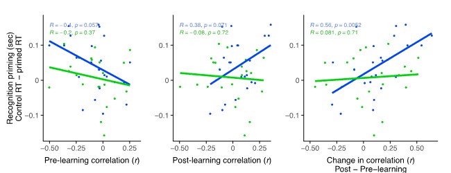
Note that the post-learning chart depicts the relationship between post-remote coupling and remote priming and between post-recent coupling and recent priming (middle). Essentially, post-recent learning coupling did not relate to priming of recently learned sequences (middle; green) while there remains a trend for a relationship between post-remote coupling and priming for remotely learned sequences (middle; blue). However, the significant relationship between coupling and priming that we reported in the paper (right, blue) is driven both by the initial negative relationship that is observed in the pre-learning scan and the positive relationship in the post-remote learning scan. This highlights the importance of using a change score, as there may be spurious initial relationships between connectivity profiles and to-be-learned information that would then mask any learning- and consolidation-related changes.
We also reasoned that if comparisons between the post-recent learning scan and the baseline scan are noisier than between the post-remote learning and baseline scan, there may be differences in the variance of the change scores across participants, such that changes in coupling from baseline to post-recent rest may be more variable than coupling from baseline to post-remote rest. We conducted F-tests to compare the variance of the change in these two hippocampal-LO correlations and found no reliable difference (ratio of difference: F(22, 22) = 0.811, p = .63).
Finally, we explored whether hippocampal-LOC coupling is more stable across participants if compared across two rest scans within the same imaging session (baseline and post-remote) versus across two scans across two separate sessions (baseline and post-recent). Interestingly, coupling was not reliably correlated across scans in either case (baseline/post-remote: r = 0.03, p = 0.89 Baseline/post-recent: r = 0.07, p = .74).
Finally, we evaluated whether hippocampal-LOC coupling was correlated across different rest scans (see Author response image 2). We reasoned that if such coupling was more correlated across baseline and post-remote scans relative to baseline and post-recent scans, that would indicate a within-session stability of participants’ connectivity profiles. At the same time, less correlation of coupling across baseline and post-recent scans would be an indication of a noisier change measure as the measure would additionally include a change in individuals’ connectivity profile over time. We found that there was no difference in the correlation of hipp-LO coupling is across sessions, and the correlation was not reliably significant for either session (baseline/post-remote: r = 0.03, p = 0.89; baseline/post-recent: r = 0.07, p = .74; difference: Steiger’s t = 0.12, p = 0.9).
Author response image 2.
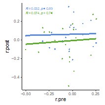
We have included the raw correlations with priming (page 25, lines 654-661, Supplemental Figure 6) as well as text describing the comparison of variances (page 25, lines 642-653). We did not add the comparison of hippocampal-LOC coupling across scans to the current manuscript, as an evaluation of stability of such coupling in the context of learning and reactivation seems out of scope of the current focus of the experiment, but we find this result to be worthy of follow-up in future work.
In summary, further analysis of our data did not reveal any indication that a comparison of rest connectivity across scan sessions inserted noise into the change score between baseline and post-recent learning scans. However, these analyses cannot fully rule that possibility out, and the current analyses do not provide concrete evidence that the post-recent learning scan comprises signals that are a mixture of processing of recent and remote sequences. We discuss these drawbacks in the Discussion (page 39, lines 1047-1070).
2) My second major concern is how the authors have operationalized integration and differentiation. The pattern similarity analysis uses an overall correspondence between the neural similarity and a predicted model as the main metric. In the predicted model, C items that are indirectly associated are more similar to one another than they are C items that are entirely unrelated. The authors are then looking at a change in correspondence (correlation) between the neural data and that prediction model from pre- to post-learning. However, a change in the degree of correspondence with the predicted matrix could be driven by either the unrelated items becoming less similar or the related ones becoming more similar (or both!). Since the interpretation in the paper focuses on change to indirectly related C items, it would be important to report those values directly. For instance, as evidence of differentiation, it would be important to show that there is a greater decrease in similarity for indirectly associated C items than it is for unrelated C items (or even a smaller increase) from pre to post, or that C items that are indirectly related are less similar than are unrelated C items post but not pre-learning. Performing this analysis would confirm that the pattern of results matches the authors' interpretation. This would also impact the interpretation of the subsequent analyses that involve the neural integration measures (e.g., correlation analyses like those on p. 16, which may or may not be driven by increased similarity among overlapping C pairs). I should add that given the specificity to the remote learning in mPFC versus recent in LOC and anterior hippocampus, it is clearly the case that something interesting is going on. However, I think we need more data to understand fully what that "something" is.
We recognize the importance of understanding whether model fits (and changes to them) are driven by similarity of overlapping pairs or non-overlapping pairs. We have modified all figures that visualize model fits to the neural integration model to separately show fits for pre- and post-learning (Figure 3 for mPFC, Supp. Figure 5 for LOC, Supp. Figure 9 for AB similarity in anterior hippocampus & LOC). We have additionally added supplemental figures to show the complete breakdown of similarity each region in a 2 (pre/post) x 2 (overlapping/non-overlapping sequence) x 2 (recent/remote) chart. We decided against including only these latter charts rather than the model fits since the model fits strike a good balance between information and readability. We have also modified text in various sections to focus on these new results.
In brief, the decrease in model fit for mPFC for the remote sequences was driven primarily by a decrease in similarity for the overlapping C items and not the non-overlapping ones (Supplementary Figure 3, page 18, lines 468-472).
Interestingly, in LOC, all C items grew more similar after learning, regardless of their overlap or learning session, but the increase in model fit for C items in the recent condition was driven by a larger increase in similarity for overlapping pairs relative to non-overlapping ones (Supp. Figure 5, page 21, lines 533-536).
We also visualized AB similarity in the anterior hippocampus and LOC in a similar fashion (Supplementary Figure 9).
We have also edited the Methods sections with updated details of these analyses (page 52, lines 1392-1397). We think that including these results considerably strengthen our claims and we are pleased to have them included.
3) The priming task occurred before the post-learning exposure phase and could have impacted the representations. More consideration of this in the paper would be useful. Most critically, since the priming task involves seeing the related C items back-to-back, it would be important to consider whether this experience could have conceivably impacted the neural integration indices. I believe it never would have been the case that unrelated C items were presented sequentially during the priming task, i.e., that related C items always appeared together in this task. I think again the specificity of the remote condition is key and perhaps the authors can leverage this to support their interpretation. Can the authors consider this possibility in the Discussion?
It's true that only C items from the same sequence were presented back-to-back during the priming task, and that this presentation may interfere with observations from the post-learning exposure scan that followed it. We agree that it is worth considering this caveat and have added language in the Discussion (page 40, lines 1071-1086). When designing the study, we reasoned that it was more important for the behavioral priming task to come before the exposure scans, as all items were shown only once in that task, whereas they were shown 4-5 times in a random order in the post-learning exposure phase. Because of this difference in presentation times, and because behavioral priming findings tend to be very sensitive, we concluded that it was more important to protect the priming task from the exposure scan instead of the reverse.
We reasoned, however, that the additional presentation of the C items in the recognition priming task would not substantially override the sequence learning, as C items were each presented 16 times in their sequence (ABC1 and ABC2 16 times each). Furthermore, as this reviewer suggests, the order of C items during recognition was the same for recent and remote conditions, so the fact that we find a selective change in neural representation for the remote condition and don’t also see that change for the recent condition is additional assurance that the recognition priming order did not substantially impact the representations.
4) For the priming task, based on the Figure 2A caption it seems as though every sequence contributes to both the control and primed conditions, but (I believe) this means that the control transition always happens first (and they are always back-to-back). Is this a concern? If RTs are changing over time (getting faster), it would be helpful to know whether the priming effects hold after controlling for trial numbers. I do not think this is a big issue because if it were, you would not expect to see the specificity of the remotely learned information. However, it would be helpful to know given the order of these conditions has to be fixed in their design.
This is a correct understanding of the trial orders in the recognition priming task. We chose to involve the baseline items in the control condition to boost power – this way, priming of each sequence could be tested, while only presenting each item once in this task, as repetition in the recognition phase would have further facilitated response times and potentially masked any priming effects. We agree that accounting for trial order would be useful here, so we ran a mixed-effects linear model to examine responses times both as a function of trial number and of priming condition (primed/control). While there is indeed a large effect of trial number such that participants got faster over time, the priming effect originally observed in the remote condition still holds at the same time. We now report this analysis in the Results section (page 14, lines 337-349 for Expt 1 and pages 14-15, lines 360-362 for Expt 2).
5) The authors should be cautious about the general conclusion that memories with overlapping temporal regularities become neurally integrated - given their findings in MPFC are more consistent with overall differentiation (though as noted above, I think we need more data on this to know for sure what is going on).
We realize this conclusion was overly simplistic and, in several places, have revised the general conclusions to be more specific about the nuanced similarity findings.
6) It would be worth stating a few more details and perhaps providing additional logic or justification in the main text about the pre- and post-exposure phases were set up and why. How many times each object was presented pre and post, and how the sequencing was determined (were any constraints put in place e.g., such that C1 and C2 did not appear close in time?). What was the cover task (I think this is important to the interpretation & so belongs in the main paper)? Were there considerations involving the fact that this is a different sequence of the same objects the participants would later be learning - e.g., interference, etc.?
These details can be found in the Methods section (pages 50-51, lines 1337-1353) and we’ve added a new summary of that section in the Results (page 17, lines 424- 425 and 432-435). In brief, a visual hash tag appeared on a small subset of images and participants pressed a button when this occurred, and C1 and C2 objects were presented in separate scans (as were A and B objects) to minimize inflated neural similarity due to temporal proximity.
Reviewer #2 (Public Review):
The manuscript by Tompary & Davachi presents results from two experiments, one behavior only and one fMRI plus behavior. They examine the important question of how to separate object memories (C1 and C2) that are never experienced together in time and become linked by shared predictive cues in a sequence (A followed by B followed by one of the C items). The authors developed an implicit priming task that provides a novel behavioral metric for such integration. They find significant C1-C2 priming for sequences that were learned 24h prior to the test, but not for recently learned sequences, suggesting that associative links between the two originally separate memories emerge over an extended period of consolidation. The fMRI study relates this behavioral integration effect to two neural metrics: pattern similarity changes in the medial prefrontal cortex (mPFC) as a measure of neural integration, and changes in hippocampal-LOC connectivity as a measure of post-learning consolidation. While fMRI patterns in mPFC overall show differentiation rather than integration (i.e., C1-C2 representational distances become larger), the authors find a robust correlation such that increasing pattern similarity in mPFC relates to stronger integration in the priming test, and this relationship is again specific to remote memories. Moreover, connectivity between the posterior hippocampus and LOC during post-learning rest is positively related to the behavioral integration effect as well as the mPFC neural similarity index, again specifically for remote memories. Overall, this is a coherent set of findings with interesting theoretical implications for consolidation theories, which will be of broad interest to the memory, learning, and predictive coding communities.
Strengths:
1) The implicit associative priming task designed for this study provides a promising new tool for assessing the formation of mnemonic links that influence behavior without explicit retrieval demands. The authors find an interesting dissociation between this implicit measure of memory integration and more commonly used explicit inference measures: a priming effect on the implicit task only evolved after a 24h consolidation period, while the ability to explicitly link the two critical object memories is present immediately after learning. While speculative at this point, these two measures thus appear to tap into neocortical and hippocampal learning processes, respectively, and this potential dissociation will be of interest to future studies investigating time-dependent integration processes in memory.
2) The experimental task is well designed for isolating pre- vs post-learning changes in neural similarity and connectivity, including important controls of baseline neural similarity and connectivity.
3) The main claim of a consolidation-dependent effect is supported by a coherent set of findings that relate behavioral integration to neural changes. The specificity of the effects on remote memories makes the results particularly interesting and compelling.
4) The authors are transparent about unexpected results, for example, the finding that overall similarity in mPFC is consistent with a differentiation rather than an integration model.
Thank you for the positive comments!
Weaknesses:
1) The sequence learning and recognition priming tasks are cleverly designed to isolate the effects of interest while controlling for potential order effects. However, due to the complex nature of the task, it is difficult for the reader to infer all the transition probabilities between item types and how they may influence the behavioral priming results. For example, baseline items (BL) are interspersed between repeated sequences during learning, and thus presumably can only occur before an A item or after a C item. This seems to create non-random predictive relationships such that C is often followed by BL, and BL by A items. If this relationship is reversed during the recognition priming task, where the sequence is always BL-C1-C2, this violation of expectations might slow down reaction times and deflate the baseline measure. It would be helpful if the manuscript explicitly reported transition probabilities for each relevant item type in the priming task relative to the sequence learning task and discussed how a match vs mismatch may influence the observed priming effects.
We have added a table of transition probabilities across the learning, recognition priming, and exposure scans (now Table 1, page 48). We have also included some additional description of the change in transition probabilities across different tasks in the Methods section. Specifically, if participants are indeed learning item types and rules about their order, then both the control and the primed conditions would violate that order. Since C1 and C2 items never appeared together, viewing C1 would give rise to an expectation of seeing a BL item, which would also be violated. This suggests that our priming effects are driven by sequence-specific relationships rather than learning of the probabilities of different item types. We’ve added this consideration to the Methods section (page 45, lines 1212-1221).
Another critical point to consider (and that the transition probabilities do not reflect) is that during learning, while C is followed either by A or BL, they are followed by different A or BL items. In contrast, a given A is always followed by the same B object, which is always followed by one of two C objects. While the order of item types is semi-predictable, the order of objects (specific items) themselves are not. This can be seen in the response times during learning, such that response times for A and BL items are always slower than for B and C items. We have explained this nuance in the figure text for Table 1.
2) The choice of what regions of interest to include in the different sets of analyses could be better motivated. For example, even though briefly discussed in the intro, it remains unclear why the posterior but not the anterior hippocampus is of interest for the connectivity analyses, and why the main target is LOC, not mPFC, given past results including from this group (Tompary & Davachi, 2017). Moreover, for readers not familiar with this literature, it would help if references were provided to suggest that a predictable > unpredictable contrast is well suited for functionally defining mPFC, as done in the present study.
We have clarified our reasoning for each of these choices throughout the manuscript and believe that our logic is now much more transparent. For an expanded reasoning of why we were motivated to look at posterior and not anterior hippocampus, see pages 6-7, lines 135-159, and our response to R2. In brief, past research focusing on post-encoding connectivity with the hippocampus suggests that posterior aspect is more likely to couple with category-selective cortex after learning neutral, non-rewarded objects much like the stimuli used in the present study.
We also clarify our reasoning for LOC over mPFC. While theoretically, mPFC is thought to be a candidate region for coupling with the hippocampus during consolidation, the bulk of empirical work to date has revealed post-encoding connectivity between the hippocampus and category-selective cortex in the ventral and occipital lobes (page 6, lines 123-134).
As for the use of the predictable > unpredictable contrast for functionally defining cortical regions, we reasoned that cortical regions that were sensitive to the temporal regularities generated by the sequences may be further involved in their offline consolidation and long-term storage (Danker & Anderson, 2010; Davachi & Danker, 2013; McClelland et al., 1995). We have added this justification to the Methods section (page 18, lines 454-460).
3) Relatedly, multiple comparison corrections should be applied in the fMRI integration and connectivity analyses whenever the same contrast is performed on multiple regions in an exploratory manner.
We now correct for multiple comparisons using Bonferroni correction, and this correction depends on the number of regions in which each analysis is conducted. Please see page 55, lines 1483-1490, in the Methods section for details of each analysis.
Reviewer #3 (Public Review):
The authors of this manuscript sought to illuminate a link between a behavioral measure of integration and neural markers of cortical integration associated with systems consolidation (post-encoding connectivity, change in representational neural overlap). To that aim, participants incidentally encoded sequences of objects in the fMRI scanner. Unbeknownst to participants, the first two objects of the presented ABC triplet sequences overlapped for a given pair of sequences. This allowed the authors to probe the integration of unique C objects that were never directly presented in the same sequence, but which shared the same preceding A and B objects. They encoded one set of objects on Day 1 (remote condition), another set of objects 24 hours later (recent condition) and tested implicit and explicit memory for the learned sequences on Day 2. They additionally collected baseline and post-encoding resting-state scans. As their measure of behavioral integration, the authors examined reaction time during an Old/New judgement task for C objects depending on if they were preceded by a C object from an overlapping sequence (primed condition) versus a baseline object. They found faster reaction times for the primed objects compared to the control condition for remote but not recently learned objects, suggesting that the C objects from overlapping sequences became integrated over time. They then examined pattern similarity in a priori ROIs as a measure of neural integration and found that participants showing evidence of integration of C objects from overlapping sequences in the medial prefrontal cortex for remotely learned objects also showed a stronger implicit priming effect between those C objects over time. When they examined the change in connectivity between their ROIs after encoding, they also found that connectivity between the posterior hippocampus and lateral occipital cortex correlated with larger priming effects for remotely learned objects, and that lateral occipital connectivity with the medial prefrontal cortex was related to neural integration of remote objects from overlapping sequences.
The authors aim to provide evidence of a relationship between behavioral and neural measures of integration with consolidation is interesting, important, and difficult to achieve given the longitudinal nature of studies required to answer this question. Strengths of this study include a creative behavioral task, and solid modelling approaches for fMRI data with careful control for several known confounds such as bold activation on pattern analysis results, motion, and physiological noise. The authors replicate their behavioral observations across two separate experiments, one of which included a large sample size, and found similar results that speak to the reliability of the observed behavioral phenomenon. In addition, they document several correlations between neural measures and task performance, lending functional significance to their neural findings.
Thank you for this positive assessment of our study!
However, this study is not without notable weaknesses that limit the strength of the manuscript. The authors report a behavioral priming effect suggestive of integration of remote but not recent memories, leading to the interpretation that the priming effect emerges with consolidation. However, they did not observe a reliable interaction between the priming condition and learning session (recent/remote) on reaction times, meaning that the priming effect for remote memories was not reliably greater than that observed for recent. In addition, the emergence of a priming effect for remote memories does not appear to be due to faster reaction times for primed targets over time (the condition of interest), but rather, slower reaction times for control items in the remote condition compared to recent. These issues limit the strength of the claim that the priming effect observed is due to C items of interest being integrated in a consolidation-dependent manner.
We acknowledge that the lack of a day by condition interaction in the behavioral priming effect should discussed and now discuss this data in a more nuanced manner. While it’s true that the priming effect emerges due to a slowing of the control items over time, this slowing is consistent with classic time-dependent effects demonstrating slower response times for more delayed memories. The fact that the response times in the primed condition does not show this slowing can be interpreted as a protection against this slowing that would otherwise occur. Please see page 29, lines 758-766, for this added discussion.
Similarly, the interactions between neural variables of interest and learning session needed to strongly show a significant consolidation-related effect in the brain were sometimes tenuous. There was no reliable difference in neural representational pattern analysis fit to a model of neural integration between the short and long delays in the medial prefrontal cortex or lateral occipital cortex, nor was the posterior hippocampus-lateral occipital cortex post-encoding connectivity correlation with subsequent priming significantly different for recent and remote memories. While the relationship between integration model fit in the medial prefrontal cortex and subsequent priming (which was significantly different from that occurring for recent memories) was one of the stronger findings of the paper in favor of a consolidation-related effect on behavior, is it possible that lack of a behavioral priming effect for recent memories due to possible issues with the control condition could mask a correlation between neural and behavioral integration in the recent memory condition?
While we acknowledge that lack of a statistically reliable interaction between neural measures and behavioral priming in many cases, we are heartened by the reliable difference in the relationship between mPFC similarity and priming over time, which was our main planned prediction. In addition to adding caveats in the discussion about the neural measures and behavioral findings in the recent condition (see our response to R1.1 and R1.4 for more details), we have added language throughout the manuscript noting the need to interpret these data with caution.
These limitations are especially notable when one considers that priming does not classically require a period of prolonged consolidation to occur, and prominent models of systems consolidation rather pertain to explicit memory. While the authors have provided evidence that neural integration in the medial prefrontal cortex, as well as post-encoding coupling between the lateral occipital cortex and posterior hippocampus, are related to faster reaction times for primed objects of overlapping sequences compared to their control condition, more work is needed to verify that the observed findings indeed reflect consolidation dependent integration as proposed.
We agree that more work is needed to provide converging evidence for these novel findings. However, we wish to counter the notion that systems consolidation models are relevant only for explicit memories. Although models of systems consolidation often mention transformations from episodic to semantic memory, the critical mechanisms that define the models involve changes in the neural ensembles of a memory that is initially laid down in the hippocampus and is taught to cortex over time. This transformation of neural traces is not specific to explicit/declarative forms of memory. For example, implicit statistical learning initially depends on intact hippocampal function (Schapiro et al., 2014) and improves over consolidation (Durrant et al., 2011, 2013; Kóbor et al., 2017).
Second, while there are many classical findings of priming during or immediately after learning, there are several instances of priming used to measure consolidation-related changes to newly learned information. For instance, priming has been used as a measure of lexical integration, demonstrating that new word learning benefits from a night of sleep (Wang et al., 2017; Gaskell et al., 2019) or a 1-week delay (Tamminen & Gaskell, 2013). The issue is not whether priming can occur immediately, it is whether priming increases with a delay.
Finally, it is helpful to think about models of memory systems that divide memory representations not by their explicit/implicit nature, but along other important dimensions such as their neural bases, their flexibility vs rigidity, and their capacity for rapid vs slow learning (Henke, 2010). Considering this evidence, we suggest that systems consolidation models are most useful when considering how transformations in the underlying neural memory representation affects its behavioral expression, rather than focusing on the extent that the memory representation is explicit or implicit.
With all this said, we have added text to the discussion reminding the reader that there was no statistically significant difference in priming as a function of the delay (page 29, lines 764 - 766). However, we are encouraged by the fact that the relationship between priming and mPFC neural similarity was significantly stronger for remotely learned objects relative to recently learned ones, as this is directly in line with systems consolidation theories.
References
Abolghasem, Z., Teng, T. H.-T., Nexha, E., Zhu, C., Jean, C. S., Castrillon, M., Che, E., Di Nallo, E. V., & Schlichting, M. L. (2023). Learning strategy differentially impacts memory connections in children and adults. Developmental Science, 26(4), e13371. https://doi.org/10.1111/desc.13371
Dobbins, I. G., Schnyer, D. M., Verfaellie, M., & Schacter, D. L. (2004). Cortical activity reductions during repetition priming can result from rapid response learning. Nature, 428(6980), 316–319. https://doi.org/10.1038/nature02400
Durrant, S. J., Cairney, S. A., & Lewis, P. A. (2013). Overnight consolidation aids the transfer of statistical knowledge from the medial temporal lobe to the striatum. Cerebral Cortex, 23(10), 2467–2478. https://doi.org/10.1093/cercor/bhs244
Durrant, S. J., Taylor, C., Cairney, S., & Lewis, P. A. (2011). Sleep-dependent consolidation of statistical learning. Neuropsychologia, 49(5), 1322–1331. https://doi.org/10.1016/j.neuropsychologia.2011.02.015
Gaskell, M. G., Cairney, S. A., & Rodd, J. M. (2019). Contextual priming of word meanings is stabilized over sleep. Cognition, 182, 109–126. https://doi.org/10.1016/j.cognition.2018.09.007
Henke, K. (2010). A model for memory systems based on processing modes rather than consciousness. Nature Reviews Neuroscience, 11(7), 523–532. https://doi.org/10.1038/nrn2850
Kóbor, A., Janacsek, K., Takács, Á., & Nemeth, D. (2017). Statistical learning leads to persistent memory: Evidence for one-year consolidation. Scientific Reports, 7(1), 760. https://doi.org/10.1038/s41598-017-00807-3
Kuhl, B. A., & Chun, M. M. (2014). Successful remembering elicits event-specific activity patterns in lateral parietal cortex. The Journal of Neuroscience, 34(23), 8051–8060. https://doi.org/10.1523/JNEUROSCI.4328-13.2014
Richter, F. R., Chanales, A. J. H., & Kuhl, B. A. (2016). Predicting the integration of overlapping memories by decoding mnemonic processing states during learning. NeuroImage, 124, Part A, 323–335. https://doi.org/10.1016/j.neuroimage.2015.08.051
Schapiro, A. C., Gregory, E., Landau, B., McCloskey, M., & Turk-Browne, N. B. (2014). The necessity of the medial-temporal lobe for statistical learning. Journal of Cognitive Neuroscience, 1–12. https://doi.org/10.1162/jocn_a_00578
Schlichting, M. L., & Preston, A. R. (2014). Memory reactivation during rest supports upcoming learning of related content. Proceedings of the National Academy of Sciences, 111(44), 15845–15850. https://doi.org/10.1073/pnas.1404396111
Smith, J. F., Alexander, G. E., Chen, K., Husain, F. T., Kim, J., Pajor, N., & Horwitz, B. (2010). Imaging systems level consolidation of novel associate memories: A longitudinal neuroimaging study. NeuroImage, 50(2), 826–836. https://doi.org/10.1016/j.neuroimage.2009.11.053
Takashima, A., Nieuwenhuis, I. L. C., Jensen, O., Talamini, L. M., Rijpkema, M., & Fernández, G. (2009). Shift from hippocampal to neocortical centered retrieval network with consolidation. The Journal of Neuroscience, 29(32), 10087–10093. https://doi.org/10.1523/JNEUROSCI.0799-09.2009
Tamminen, J., & Gaskell, M. G. (2013). Novel word integration in the mental lexicon: Evidence from unmasked and masked semantic priming. The Quarterly Journal of Experimental Psychology, 66(5), 1001–1025. https://doi.org/10.1080/17470218.2012.724694
van Kesteren, M. T. R. van, Fernández, G., Norris, D. G., & Hermans, E. J. (2010). Persistent schema-dependent hippocampal-neocortical connectivity during memory encoding and postencoding rest in humans. Proceedings of the National Academy of Sciences, 107(16), 7550–7555. https://doi.org/10.1073/pnas.0914892107
Wang, H.-C., Savage, G., Gaskell, M. G., Paulin, T., Robidoux, S., & Castles, A. (2017). Bedding down new words: Sleep promotes the emergence of lexical competition in visual word recognition. Psychonomic Bulletin & Review, 24(4), 1186–1193. https://doi.org/10.3758/s13423-016-1182-7
Author Response:
Reviewer #3:
The authors modified a previously reported hybrid cytochrome bcc-aa3 supercomplex, consisting of bcc from M. tuberculosis and aa3 from M. smegmatis, (Kim et al 2015) by appending an affinity tag facilitating purification. The cryo-EM experiments are based on the authors' earlier work (Gong et al. 2018) on the structure of the bcc-aa3 supercomplex from M. smegmatis. The authors then determine the structure of the bcc part alone and in complex with Q203 and TB47.
The manuscript is well written and the obtained results are presented in a concise, clear-cut manner. In general, the data support the conclusions drawn.
We thank the reviewer for this evaluation.
To this reviewer, the following points are unclear:
- The purified enzyme elutes from the gel filtration column as one peak, but there seems to be no information given on the subunit composition and the enzymatic activity of the purified hybrid cytochrome bcc-aa3 supercomplex.
See answers to Question 1 from the major Essential Revisions and Question 1 from the minor Essential Revisions.
"We have now shown that the purified chimeric supercomplex is a functional assembly with a (mean ± s.d., n = 4), in agreement with the previous study that shows M. tuberculosis CIII can functionally complement native M. smegmatis CIII and maintain the growth of M. smegmatis (Kim et al., 2015). The in vitro inhibitions of this enzyme by Q203 and TB47 was determined by means of an DMNQH2/oxygen oxidoreductase activity assay. In the assay, 500 nM Q203 or TB47 was chosen, which is close to the median inhibitory concentration (IC50) obtained from the menadiol-induced oxygen consumption in our previous study (Gong et al., 2018). After addition of Q203 and TB47, the values of turnover number of the hybrid supercomplex are reduced to 5.8 +/- 2.4 e-s-1 (Figure 4-figure supplement 4) and 5.1 +/- 2.9 e-s-1 (Figure 5-figure supplement 4) respectively, from 23.3 +/- 2.4 e-s-1. We have incorporated this new data into the text (lines 90-93, 187-189, 206-209)."
"The subunit composition of the purified enzyme has now been provided in Figure 2-figure supplement 1."
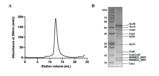
- It is unclear what is the conclusion of the structure comparison (Fig 6) is regarding the affinity of Q203 for M. smegmatis.
The structural comparison indicates that Q203 should have a similar binding mechanism and a similar effect on the activity of cytochrome bcc from M. smegmatis and M. tuberculosis. This is in good agreement with previous antimycobacterial activity data and inhibition data for the bcc complexes from M. smegmatis and M. tuberculosis (Gong et al., 2018; Lu et al., 2018a). These have now been incorporated into the revised manuscript (line 223-227).
Author Response
Reviewer #1 (Public Review):
This study used a multi-day learning paradigm combined with fMRI to reveal neural changes reflecting the learning of new (arbitrary) shape-sound associations. In the scanner, the shapes and sounds are presented separately and together, both before and after learning. When they are presented together, they can be either consistent or inconsistent with the learned associations. The analyses focus on auditory and visual cortices, as well as the object-selective cortex (LOC) and anterior temporal lobe regions (temporal pole (TP) and perirhinal cortex (PRC)). Results revealed several learning-induced changes, particularly in the anterior temporal lobe regions. First, the LOC and PRC showed a reduced bias to shapes vs sounds (presented separately) after learning. Second, the TP responded more strongly to incongruent than congruent shape-sound pairs after learning. Third, the similarity of TP activity patterns to sounds and shapes (presented separately) was increased for non-matching shape-sound comparisons after learning. Fourth, when comparing the pattern similarity of individual features to combined shape-sound stimuli, the PRC showed a reduced bias towards visual features after learning. Finally, comparing patterns to combined shape-sound stimuli before and after learning revealed a reduced (and negative) similarity for incongruent combinations in PRC. These results are all interpreted as evidence for an explicit integrative code of newly learned multimodal objects, in which the whole is different from the sum of the parts.
The study has many strengths. It addresses a fundamental question that is of broad interest, the learning paradigm is well-designed and controlled, and the stimuli are real 3D stimuli that participants interact with. The manuscript is well written and the figures are very informative, clearly illustrating the analyses performed.
There are also some weaknesses. The sample size (N=17) is small for detecting the subtle effects of learning. Most of the statistical analyses are not corrected for multiple comparisons (ROIs), and the specificity of the key results to specific regions is also not tested. Furthermore, the evidence for an integrative representation is rather indirect, and alternative interpretations for these results are not considered.
We thank the reviewer for their careful reading and the positive comments on our manuscript. As suggested, we have conducted additional analyses of theoretically-motivated ROIs and have found that temporal pole and perirhinal cortex are the only regions to show the key experience-dependent transformations. We are much more cautious with respect to multiple comparisons, and have removed a series of post hoc across-ROI comparisons that were irrelevant to the key questions of the present manuscript. The revised manuscript now includes much more discussion about alternative interpretations as suggested by the reviewer (and also by the other reviewers).
Additionally, we looked into scanning more participants, but our scanner has since had a full upgrade and the sequence used in the current study is no longer supported by our scanner. However, we note that while most analyses contain 17 participants, we employed a within-subject learning design that is not typically used in fMRI experiments and increases our power to detect an effect. This is supported by the robust effect size of the behavioural data, whereby 17 out of 18 participants revealed a learning effect (Cohen’s D = 1.28) and which was replicated in a follow-up experiment with a larger sample size.
We address the other reviewer comments point-by-point in the below.
Reviewer #2 (Public Review):
Li et al. used a four-day fMRI design to investigate how unimodal feature information is combined, integrated, or abstracted to form a multimodal object representation. The experimental question is of great interest and understanding how the human brain combines featural information to form complex representations is relevant for a wide range of researchers in neuroscience, cognitive science, and AI. While most fMRI research on object representations is limited to visual information, the authors examined how visual and auditory information is integrated to form a multimodal object representation. The experimental design is elegant and clever. Three visual shapes and three auditory sounds were used as the unimodal features; the visual shapes were used to create 3D-printed objects. On Day 1, the participants interacted with the 3D objects to learn the visual features, but the objects were not paired with the auditory features, which were played separately. On Day 2, participants were scanned with fMRI while they were exposed to the unimodal visual and auditory features as well as pairs of visual-auditory cues. On Day 3, participants again interacted with the 3D objects but now each was paired with one of the three sounds that played from an internal speaker. On Day 4, participants completed the same fMRI scanning runs they completed on Day 2, except now some visual-auditory feature pairs corresponded with Congruent (learned) objects, and some with Incongruent (unlearned) objects. Using the same fMRI design on Days 2 and 4 enables a well-controlled comparison between feature- and object-evoked neural representations before and after learning. The notable results corresponded to findings in the perirhinal cortex and temporal pole. The authors report (1) that a visual bias on Day 2 for unimodal features in the perirhinal cortex was attenuated after learning on Day 4, (2) a decreased univariate response to congruent vs. incongruent visual-auditory objects in the temporal pole on Day 4, (3) decreased pattern similarity between congruent vs. incongruent pairs of visual and auditory unimodal features in the temporal pole on Day 4, (4) in the perirhinal cortex, visual unimodal features on Day 2 do not correlate with their respective visual-auditory objects on Day 4, and (5) in the perirhinal cortex, multimodal object representations across Days 2 and 4 are uncorrelated for congruent objects and anticorrelated for incongruent. The authors claim that each of these results supports the theory that multimodal objects are represented in an "explicit integrative" code separate from feature representations. While these data are valuable and the results are interesting, the authors' claims are not well supported by their findings.
We thank the reviewer for the careful reading of our manuscript and positive comments. Overall, we now stay closer to the data when describing the results and provide our interpretation of these results in the discussion section while remaining open to alternative interpretations (as also suggested by Reviewer 1).
(1) In the introduction, the authors contrast two theories: (a) multimodal objects are represented in the co-activation of unimodal features, and (b) multimodal objects are represented in an explicit integrative code such that the whole is different than the sum of its parts. However, the distinction between these two theories is not straightforward. An explanation of what is precisely meant by "explicit" and "integrative" would clarify the authors' theoretical stance. Perhaps we can assume that an "explicit" representation is a new representation that is created to represent a multimodal object. What is meant by "integrative" is more ambiguous-unimodal features could be integrated within a representation in a manner that preserves the decodability of the unimodal features, or alternatively the multimodal representation could be completely abstracted away from the constituent features such that the features are no longer decodable. Even if the object representation is "explicit" and distinct from the unimodal feature representations, it can in theory still contain featural information, though perhaps warped or transformed. The authors do not clearly commit to a degree of featural abstraction in their theory of "explicit integrative" multimodal object representations which makes it difficult to assess the validity of their claims.
Due to its ambiguity, we removed the term “explicit” and now make it clear that our central question was whether crossmodal object representations require only unimodal feature-level representations (e.g., frogs are created from only the combination of shape and sound) or whether crossmodal object representations also rely on an integrative code distinct from the unimodal features (e.g., there is something more to “frog” than its original shape and sound). We now clarify this in the revised manuscript.
“One theoretical view from the cognitive sciences suggests that crossmodal objects are built from component unimodal features represented across distributed sensory regions.8 Under this view, when a child thinks about “frog”, the visual cortex represents the appearance of the shape of the frog whereas the auditory cortex represents the croaking sound. Alternatively, other theoretical views predict that multisensory objects are not only built from their component unimodal sensory features, but that there is also a crossmodal integrative code that is different from the sum of these parts.9,10,11,12,13 These latter views propose that anterior temporal lobe structures can act as a polymodal “hub” that combines separate features into integrated wholes.9,11,14,15” – pg. 4
For this reason, we designed our paradigm to equate the unimodal representations, such that neural differences between the congruent and incongruent conditions provide evidence for a crossmodal integrative code different from the unimodal features (because the unimodal features are equated by default in the design).
“Critically, our four-day learning task allowed us to isolate any neural activity associated with integrative coding in anterior temporal lobe structures that emerges with experience and differs from the neural patterns recorded at baseline. The learned and non-learned crossmodal objects were constructed from the same set of three validated shape and sound features, ensuring that factors such as familiarity with the unimodal features, subjective similarity, and feature identity were tightly controlled (Figure 2). If the mind represented crossmodal objects entirely as the reactivation of unimodal shapes and sounds (i.e., objects are constructed from their parts), then there should be no difference between the learned and non-learned objects (because they were created from the same three shapes and sounds). By contrast, if the mind represented crossmodal objects as something over and above their component features (i.e., representations for crossmodal objects rely on integrative coding that is different from the sum of their parts), then there should be behavioral and neural differences between learned and non-learned crossmodal objects (because the only difference across the objects is the learned relationship between the parts). Furthermore, this design allowed us to determine the relationship between the object representation acquired after crossmodal learning and the unimodal feature representations acquired before crossmodal learning. That is, we could examine whether learning led to abstraction of the object representations such that it no longer resembled the unimodal feature representations.” – pg. 5
Furthermore, we agree with the reviewer that our definition and methodological design does not directly capture the structure of the integrative code. With experience, the unimodal feature representations may be completely abstracted away, warped, or changed in a nonlinear transformation. We suggest that crossmodal learning forms an integrative code that is different from the original unimodal representations in the anterior temporal lobes, however, we agree that future work is needed to more directly capture the structure of the integrative code that emerges with experience.
“In our task, participants had to differentiate congruent and incongruent objects constructed from the same three shape and sound features (Figure 2). An efficient way to solve this task would be to form distinct object-level outputs from the overlapping unimodal feature-level inputs such that congruent objects are made to be orthogonal from the representations before learning (i.e., measured as pattern similarity equal to 0 in the perirhinal cortex; Figure 5b, 6, Supplemental Figure S5), whereas non-learned incongruent objects could be made to be dissimilar from the representations before learning (i.e., anticorrelation, measured as patten similarity less than 0 in the perirhinal cortex; Figure 6). Because our paradigm could decouple neural responses to the learned object representations (on Day 4) from the original component unimodal features at baseline (on Day 2), these results could be taken as evidence of pattern separation in the human perirhinal cortex.11,12 However, our pattern of results could also be explained by other types of crossmodal integrative coding. For example, incongruent object representations may be less stable than congruent object representations, such that incongruent objects representation are warped to a greater extent than congruent objects (Figure 6).” – pg. 18
“As one solution to the crossmodal binding problem, we suggest that the temporal pole and perirhinal cortex form unique crossmodal object representations that are different from the distributed features in sensory cortex (Figure 4, 5, 6, Supplemental Figure S5). However, the nature by which the integrative code is structured and formed in the temporal pole and perirhinal cortex following crossmodal experience – such as through transformations, warping, or other factors – is an open question and an important area for future investigation.” – pg. 18
(2) After participants learned the multimodal objects, the authors report a decreased univariate response to congruent visual-auditory objects relative to incongruent objects in the temporal pole. This is claimed to support the existence of an explicit, integrative code for multimodal objects. Given the number of alternative explanations for this finding, this claim seems unwarranted. A simpler interpretation of these results is that the temporal pole is responding to the novelty of the incongruent visual-auditory objects. If there is in fact an explicit, integrative multimodal object representation in the temporal pole, it is unclear why this would manifest in a decreased univariate response.
We thank the reviewer for identifying this issue. Our behavioural design controls unimodal feature-level novelty but allows object-level novelty to differ. Thus, neural differences between the congruent and incongruent conditions reflects sensitivity to the object-level differences between the combination of shape and sound. However, we agree that there are multiple interpretations regarding the nature of how the integrative code is structured in the temporal pole and perirhinal cortex. We have removed the interpretation highlighted by the reviewer from the results. Instead, we now provide our preferred interpretation in the discussion, while acknowledging the other possibilities that the reviewer mentions.
As one possibility, these results in temporal pole may reflect “conceptual combination”. “hummingbird” – a congruent pairing – may require less neural resources than an incongruent pairing such as “bark-frog”.
“Furthermore, these distinct anterior temporal lobe structures may be involved with integrative coding in different ways. For example, the crossmodal object representations measured after learning were found to be related to the component unimodal feature representations measured before learning in the temporal pole but not the perirhinal cortex (Figure 5, 6, Supplemental Figure S5). Moreover, pattern similarity for congruent shape-sound pairs were lower than the pattern similarity for incongruent shape-sound pairs after crossmodal learning in the temporal pole but not the perirhinal cortex (Figure 4b, Supplemental Figure S3a). As one interpretation of this pattern of results, the temporal pole may represent new crossmodal objects by combining previously learned knowledge. 8,9,10,11,13,14,15,33 Specifically, research into conceptual combination has linked the anterior temporal lobes to compound object concepts such as “hummingbird”.34,35,36 For example, participants during our task may have represented the sound-based “humming” concept and visually-based “bird” concept on Day 1, forming the crossmodal “hummingbird” concept on Day 3; Figure 1, 2, which may recruit less activity in temporal pole than an incongruent pairing such as “barking-frog”. For these reasons, the temporal pole may form a crossmodal object code based on pre-existing knowledge, resulting in reduced neural activity (Figure 3d) and pattern similarity towards features associated with learned objects (Figure 4b).”– pg. 18
(3) The authors ran a neural pattern similarity analysis on the unimodal features before and after multimodal object learning. They found that the similarity between visual and auditory features that composed congruent objects decreased in the temporal pole after multimodal object learning. This was interpreted to reflect an explicit integrative code for multimodal objects, though it is not clear why. First, behavioral data show that participants reported increased similarity between the visual and auditory unimodal features within congruent objects after learning, the opposite of what was found in the temporal pole. Second, it is unclear why an analysis of the unimodal features would be interpreted to reflect the nature of the multimodal object representations. Since the same features corresponded with both congruent and incongruent objects, the nature of the feature representations cannot be interpreted to reflect the nature of the object representations per se. Third, using unimodal feature representations to make claims about object representations seems to contradict the theoretical claim that explicit, integrative object representations are distinct from unimodal features. If the learned multimodal object representation exists separately from the unimodal feature representations, there is no reason why the unimodal features themselves would be influenced by the formation of the object representation. Instead, these results seem to more strongly support the theory that multimodal object learning results in a transformation or warping of feature space.
We apologize for the lack of clarity. We have now overhauled this aspect of our manuscript in an attempt to better highlight key aspects of our experimental design. In particular, because the unimodal features composing the congruent and incongruent objects were equated, neural differences between these conditions would provide evidence for an experience-dependent crossmodal integrative code that is different from its component unimodal features.
Related to the second and third points, we were looking at the extent to which the original unimodal representations change with crossmodal learning. Before crossmodal learning, we found that the perirhinal cortex tracked the similarity between the individual visual shape features and the crossmodal objects that were composed of those visual shapes – however, there was no evidence that perirhinal cortex was tracking the unimodal sound features on those crossmodal objects. After crossmodal learning, we see that this visual shape bias in perirhinal cortex was no longer present – that is, the representation in perirhinal cortex started to look less like the visual features that comprise the objects. Thus, crossmodal learning transformed the perirhinal representations so that they were no longer predominantly grounded in a single visual modality, which may be a mechanism by which object concepts gain their abstraction. We have now tried to be clearer about this interpretation throughout the paper.
Notably, we suggest that experience may change both the crossmodal object representations, as well as the unimodal feature representations. For example, we have previously shown that unimodal visual features are influenced by experience in parallel with the representation of the conjunction (e.g., Liang et al., 2020; Cerebral Cortex). Nevertheless, we remain open to the myriad possible structures of the integrative code that might emerge with experience.
We now clarify these points throughout the manuscript. For example:
“We then examined whether the original representations would change after participants learned how the features were paired together to make specific crossmodal objects, conducting the same analysis described above after crossmodal learning had taken place (Figure 5b). With this analysis, we sought to measure the relationship between the representation for the learned crossmodal object and the original baseline representation for the unimodal features. More specifically, the voxel-wise activity for unimodal feature runs before crossmodal learning was correlated to the voxel-wise activity for crossmodal object runs after crossmodal learning (Figure 5b). Another linear mixed model which included modality as a fixed factor within each ROI revealed that the perirhinal cortex was no longer biased towards visual shape after crossmodal learning (F1,32 = 0.12, p = 0.73), whereas the temporal pole, LOC, V1, and A1 remained biased towards either visual shape or sound (F1,30-32 between 16.20 and 73.42, all p < 0.001, η2 between 0.35 and 0.70).” – pg. 14
“To investigate this effect in perirhinal cortex more specifically, we conducted a linear mixed model to directly compare the change in the visual bias of perirhinal representations from before crossmodal learning to after crossmodal learning (green regions in Figure 5a vs. 5b). Specifically, the linear mixed model included learning day (before vs. after crossmodal learning) and modality (visual feature match to crossmodal object vs. sound feature match to crossmodal object). Results revealed a significant interaction between learning day and modality in the perirhinal cortex (F1,775 = 5.56, p = 0.019, η2 = 0.071), meaning that the baseline visual shape bias observed in perirhinal cortex (green region of Figure 5a) was significantly attenuated with experience (green region of Figure 5b). After crossmodal learning, a given shape no longer invoked significant pattern similarity between objects that had the same shape but differed in terms of what they sounded like. Taken together, these results suggest that prior to learning the crossmodal objects, the perirhinal cortex had a default bias toward representing the visual shape information and was not representing sound information of the crossmodal objects. After crossmodal learning, however, the visual shape bias in perirhinal cortex was no longer present. That is, with crossmodal learning, the representations within perirhinal cortex started to look less like the visual features that comprised the crossmodal objects, providing evidence that the perirhinal representations were no longer predominantly grounded in the visual modality.” – pg. 13
“Importantly, the initial visual shape bias observed in the perirhinal cortex was attenuated by experience (Figure 5, Supplemental Figure S5), suggesting that the perirhinal representations had become abstracted and were no longer predominantly grounded in a single modality after crossmodal learning. One possibility may be that the perirhinal cortex is by default visually driven as an extension to the ventral visual stream,10,11,12 but can act as a polymodal “hub” region for additional crossmodal input following learning.” – pg. 19
(4) The most compelling evidence the authors provide for their theoretical claims is the finding that, in the perirhinal cortex, the unimodal feature representations on Day 2 do not correlate with the multimodal objects they comprise on Day 4. This suggests that the learned multimodal object representations are not combinations of their unimodal features. If unimodal features are not decodable within the congruent object representations, this would support the authors' explicit integrative hypothesis. However, the analyses provided do not go all the way in convincing the reader of this claim. First, the analyses reported do not differentiate between congruent and incongruent objects. If this result in the perirhinal cortex reflects the formation of new multimodal object representations, it should only be true for congruent objects but not incongruent objects. Since the analyses combine congruent and incongruent objects it is not possible to know whether this was the case. Second, just because feature representations on Day 2 do not correlate with multimodal object patterns on Day 4 does not mean that the object representations on Day 4 do not contain featural information. This could be directly tested by correlating feature representations on Day 4 with congruent vs. incongruent object representations on Day 4. It could be that representations in the perirhinal cortex are not stable over time and all representations-including unimodal feature representations-shift between sessions, which could explain these results yet not entail the existence of abstracted object representations.
We thank the reviewer for this suggestion and have conducted the two additional analyses. Specifically, we split the congruent and incongruent conditions and also investigated correlations between unimodal representations on Day 4 with crossmodal object representations on Day 4. There was no significant interaction between modality and congruency in any ROI across or within learning days. One possible explanation for these findings is that both congruent and incongruent crossmodal objects are represented differently from their underlying unimodal features, and all of these representations can transform with experience.
However, the new analyses also revealed that perirhinal cortex was the only region without a modality-specific bias after crossmodal learning (e.g., Day 4 Unimodal Feature runs x Day 4 Crossmodal Object runs; now shown in Supplemental Figure S5). Overall, these results are consistent with the notion of a crossmodal integrative code in perirhinal cortex that has changed with experience and is different from the component unimodal features. Nevertheless, we explore alternative interpretations for how the crossmodal code emerges with experience in the discussion.
“To examine whether these results differed by congruency (i.e., whether any modality-specific biases differed as a function of whether the object was congruent or incongruent), we conducted exploratory linear mixed models for each of the five a priori ROIs across learning days. More specifically, we correlated: 1) the voxel-wise activity for Unimodal Feature Runs before crossmodal learning to the voxel-wise activity for Crossmodal Object Runs before crossmodal learning (Day 2 vs. Day 2), 2) the voxel-wise activity for Unimodal Feature Runs before crossmodal learning to the voxel-wise activity for Crossmodal Object Runs after crossmodal learning (Day 2 vs Day 4), and 3) the voxel-wise activity for Unimodal Feature Runs after crossmodal learning to the voxel-wise activity for Crossmodal Object Runs after crossmodal learning (Day 4 vs Day 4). For each of the three analyses described, we then conducted separate linear mixed models which included modality (visual feature match to crossmodal object vs. sound feature match to crossmodal object) and congruency (congruent vs. incongruent)….There was no significant relationship between modality and congruency in any ROI between Day 2 and Day 2 (F1,346-368 between 0.00 and 1.06, p between 0.30 and 0.99), between Day 2 and Day 4 (F1,346-368 between 0.021 and 0.91, p between 0.34 and 0.89), or between Day 4 and Day 4 (F1,346-368 between 0.01 and 3.05, p between 0.082 and 0.93). However, exploratory analyses revealed that perirhinal cortex was the only region without a modality-specific bias and where the unimodal feature runs were not significantly correlated to the crossmodal object runs after crossmodal learning (Supplemental Figure S5).” – pg. 14
“Taken together, the overall pattern of results suggests that representations of the crossmodal objects in perirhinal cortex were heavily influenced by their consistent visual features before crossmodal learning. However, the crossmodal object representations were no longer influenced by the component visual features after crossmodal learning (Figure 5, Supplemental Figure S5). Additional exploratory analyses did not find evidence of experience-dependent changes in the hippocampus or inferior parietal lobes (Supplemental Figure S4c-e).” – pg. 14
“The voxel-wise matrix for Unimodal Feature runs on Day 4 were correlated to the voxel-wise matrix for Crossmodal Object runs on Day 4 (see Figure 5 in the main text for an example). We compared the average pattern similarity (z-transformed Pearson correlation) between shape (blue) and sound (orange) features specifically after crossmodal learning. Consistent with Figure 5b, perirhinal cortex was the only region without a modality-specific bias. Furthermore, perirhinal cortex was the only region where the representations of both the visual and sound features were not significantly correlated to the crossmodal objects. By contrast, every other region maintained a modality-specific bias for either the visual or sound features. These results suggest that perirhinal cortex representations were transformed with experience, such that the initial visual shape representations (Figure 5a) were no longer grounded in a single modality after crossmodal learning. Furthermore, these results suggest that crossmodal learning formed an integrative code different from the unimodal features in perirhinal cortex, as the visual and sound features were not significantly correlated with the crossmodal objects. * p < 0.05, ** p < 0.01, *** p < 0.001. Horizontal lines within brain regions indicate a significant main effect of modality. Vertical asterisks denote pattern similarity comparisons relative to 0.” – Supplemental Figure S5
“We found that the temporal pole and perirhinal cortex – two anterior temporal lobe structures – came to represent new crossmodal object concepts with learning, such that the acquired crossmodal object representations were different from the representation of the constituent unimodal features (Figure 5, 6). Intriguingly, the perirhinal cortex was by default biased towards visual shape, but that this initial visual bias was attenuated with experience (Figure 3c, 5, Supplemental Figure S5). Within the perirhinal cortex, the acquired crossmodal object concepts (measured after crossmodal learning) became less similar to their original component unimodal features (measured at baseline before crossmodal learning); Figure 5, 6, Supplemental Figure S5. This is consistent with the idea that object representations in perirhinal cortex integrate the component sensory features into a whole that is different from the sum of the component parts, which might be a mechanism by which object concepts obtain their abstraction…. As one solution to the crossmodal binding problem, we suggest that the temporal pole and perirhinal cortex form unique crossmodal object representations that are different from the distributed features in sensory cortex (Figure 4, 5, 6, Supplemental Figure S5). However, the nature by which the integrative code is structured and formed in the temporal pole and perirhinal cortex following crossmodal experience – such as through transformations, warping, or other factors – is an open question and an important area for future investigation.” – pg. 18
In sum, the authors have collected a fantastic dataset that has the potential to answer questions about the formation of multimodal object representations in the brain. A more precise delineation of different theoretical accounts and additional analyses are needed to provide convincing support for the theory that “explicit integrative” multimodal object representations are formed during learning.
We thank the reviewer for the positive comments and helpful feedback. We hope that our changes to our wording and clarifications to our methodology now more clearly supports the central goal of our study: to find evidence of crossmodal integrative coding different from the original unimodal feature parts in anterior temporal lobe structures. We furthermore agree that future research is needed to delineate the structure of the integrative code that emerges with experience in the anterior temporal lobes.
Reviewer #3 (Public Review):
This paper uses behavior and functional brain imaging to understand how neural and cognitive representations of visual and auditory stimuli change as participants learn associations among them. Prior work suggests that areas in the anterior temporal (ATL) and perirhinal cortex play an important role in learning/representing cross-modal associations, but the hypothesis has not been directly tested by evaluating behavior and functional imaging before and after learning cross- modal associations. The results show that such learning changes both the perceived similarities amongst stimuli and the neural responses generated within ATL and perirhinal regions, providing novel support for the view that cross-modal learning leads to a representational change in these regions.
This work has several strengths. It tackles an important question for current theories of object representation in the mind and brain in a novel and quite direct fashion, by studying how these representations change with cross-modal learning. As the authors note, little work has directly assessed representational change in ATL following such learning, despite the widespread view that ATL is critical for such representation. Indeed, such direct assessment poses several methodological challenges, which the authors have met with an ingenious experimental design. The experiment allows the authors to maintain tight control over both the familiarity and the perceived similarities amongst the shapes and sounds that comprise their stimuli so that the observed changes across sessions must reflect learned cross-modal associations among these. I especially appreciated the creation of physical objects that participants can explore and the approach to learning in which shapes and sounds are initially experienced independently and later in an associated fashion. In using multi-echo MRI to resolve signals in ventral ATL, the authors have minimized a key challenge facing much work in this area (namely the poor SNR yielded by standard acquisition sequences in ventral ATL). The use of both univariate and multivariate techniques was well-motivated and helpful in testing the central questions. The manuscript is, for the most part, clearly written, and nicely connects the current work to important questions in two literatures, specifically (1) the hypothesized role of the perirhinal cortex in representing/learning complex conjunctions of features and (2) the tension between purely embodied approaches to semantic representation vs the view that ATL regions encode important amodal/crossmodal structure.
There are some places in the manuscript that would benefit from further explanation and methodological detail. I also had some questions about the results themselves and what they signify about the roles of ATL and the perirhinal cortex in object representation.
We thank the reviewer for their positive feedback and address the comments in the below point-by-point responses.
(A) I found the terms "features" and "objects" to be confusing as used throughout the manuscript, and sometimes inconsistent. I think by "features" the authors mean the shape and sound stimuli in their experiment. I think by "object" the authors usually mean the conjunction of a shape with a sound---for instance, when a shape and sound are simultaneously experienced in the scanner, or when the participant presses a button on the shape and hears the sound. The confusion comes partly because shapes are often described as being composed of features, not features in and of themselves. (The same is sometimes true of sounds). So when reading "features" I kept thinking the paper referred to the elements that went together to comprise a shape. It also comes from ambiguous use of the word object, which might refer to (a) the 3D- printed item that people play with, which is an object, or (b) a visually-presented shape (for instance, the localizer involved comparing an "object" to a "phase-scrambled" stimulus---here I assume "object" refers to an intact visual stimulus and not the joint presentation of visual and auditory items). I think the design, stimuli, and results would be easier for a naive reader to follow if the authors used the terms "unimodal representation" to refer to cases where only visual or auditory input is presented, and "cross-modal" or "conjoint" representation when both are present.
We thank the reviewer for this suggestion and agree. We have replaced the terms “features” and “objects” with “unimodal” and “crossmodal” in the title, text, and figures throughout the manuscript for consistency (i.e., “crossmodal binding problem”). To simplify the terminology, we have also removed the localizer results.
(B) There are a few places where I wasn't sure what exactly was done, and where the methods lacked sufficient detail for another scientist to replicate what was done. Specifically:
(1) The behavioral study assessing perceptual similarity between visual and auditory stimuli was unclear. The procedure, stimuli, number of trials, etc, should be explained in sufficient detail in methods to allow replication. The results of the study should also minimally be reported in the supplementary information. Without an understanding of how these studies were carried out, it was very difficult to understand the observed pattern of behavioral change. For instance, I initially thought separate behavioral blocks were carried out for visual versus auditory stimuli, each presented in isolation; however, the effects contrast congruent and incongruent stimuli, which suggests these decisions must have been made for the conjoint presentation of both modalities. I'm still not sure how this worked. Additionally, the manuscript makes a brief mention that similarity judgments were made in the context of "all stimuli," but I didn't understand what that meant. Similarity ratings are hugely sensitive to the contrast set with which items appear, so clarity on these points is pretty important. A strength of the design is the contention that shape and sound stimuli were psychophysically matched, so it is important to show the reader how this was done and what the results were.
We agree and apologize for the lack of sufficient detail in the original manuscript. We now include much more detail about the similarity rating task. The methodology and results of the behavioral rating experiments are now shown in Supplemental Figure S1. In Figure S1a, the similarity ratings are visualized on a multidimensional scaling plot. The triangular geometry for shape (blue) and sound (red) indicate that the subjective similarity was equated within each unimodal feature across individual participants. Quantitatively, there was no difference in similarity between the congruent and incongruent pairings in Figure S1b and Figure S1c prior to crossmodal learning. In addition to providing more information on these methods in the Supplemental Information, we also now provide a more detailed description of the task in the manuscript itself. For convenience, we reproduce these sections below.
“Pairwise Similarity Task. Using the same task as the stimulus validation procedure (Supplemental Figure S1a), participants provided similarity ratings for all combinations of the 3 validated shapes and 3 validated sounds (each of the six features were rated in the context of every other feature in the set, with 4 repeats of the same feature, for a total of 72 trials). More specifically, three stimuli were displayed on each trial, with one at the top and two at the bottom of the screen in the same procedure as we have used previously27. The 3D shapes were visually displayed as a photo, whereas sounds were displayed on screen in a box that could be played over headphones when clicked with the mouse. The participant made an initial judgment by selecting the more similar stimulus on the bottom relative to the stimulus on the top. Afterwards, the participant made a similarity rating between each bottom stimulus with the top stimulus from 0 being no similarity to 5 being identical. This procedure ensured that ratings were made relative to all other stimuli in the set.”– pg. 28
“Pairwise similarity task and results. In the initial stimulus validation experiment, participants provided pairwise ratings for 5 sounds and 3 shapes. The shapes were equated in their subjective similarity that had been selected from a well-characterized perceptually uniform stimulus space27 and the pairwise ratings followed the same procedure as described in ref 27. Based on this initial experiment, we then selected the 3 sounds from the that were most closely equated in their subjective similarity. (a) 3D-printed shapes were displayed as images, whereas sounds were displayed in a box that could be played when clicked by the participant. Ratings were averaged to produce a similarity matrix for each participant, and then averaged to produce a group-level similarity matrix. Shown as triangular representational geometries recovered from multidimensional scaling in the above, shapes (blue) and sounds (orange) were approximately equated in their subjective similarity. These features were then used in the four-day crossmodal learning task. (b) Behavioral results from the four-day crossmodal learning task paired with multi-echo fMRI described in the main text. Before crossmodal learning, there was no difference in similarity between shape and sound features associated with congruent objects compared to incongruent objects – indicating that similarity was controlled at the unimodal feature-level. After crossmodal learning, we observed a robust shift in the magnitude of similarity. The shape and sound features associated with congruent objects were now significantly more similar than the same shape and sound features associated with incongruent objects (p < 0.001), evidence that crossmodal learning changed how participants experienced the unimodal features (observed in 17/18 participants). (c) We replicated this learning-related shift in pattern similarity with a larger sample size (n = 44; observed in 38/44 participants). *** denotes p < 0.001. Horizontal lines denote the comparison of congruent vs. incongruent conditions. – Supplemental Figure S1
(2) The experiences through which participants learned/experienced the shapes and sounds were unclear. The methods mention that they had one minute to explore/palpate each shape and that these experiences were interleaved with other tasks, but it is not clear what the other tasks were, how many such exploration experiences occurred, or how long the total learning time was. The manuscript also mentions that participants learn the shape-sound associations with 100% accuracy but it isn't clear how that was assessed. These details are important partly b/c it seems like very minimal experience to change neural representations in the cortex.
We apologize for the lack of detail and agree with the reviewer’s suggestions – we now include much more information in the methods section. Each behavioral day required about 1 hour of total time to complete, and indeed, participants rapidly learned their associations with minimal experience. For example:
“Behavioral Tasks. On each behavioral day (Day 1 and Day 3; Figure 2), participants completed the following tasks, in this order: Exploration Phase, one Unimodal Feature 1-back run (26 trials), Exploration Phase, one Crossmodal 1-back run (26 trials), Exploration Phase, Pairwise Similarity Task (24 trials), Exploration Phase, Pairwise Similarity Task (24 trials), Exploration Phase, Pairwise Similarity Task (24 trials), and finally, Exploration Phase. To verify learning on Day 3, participants also additionally completed a Learning Verification Task at the end of the session. – pg. 27
“The overall procedure ensured that participants extensively explored the unimodal features on Day 1 and the crossmodal objects on Day 3. The Unimodal Feature and the Crossmodal Object 1-back runs administered on Day 1 and Day 3 served as practice for the neuroimaging sessions on Day 2 and Day 4, during which these 1-back tasks were completed. Each behavioral session required less than 1 hour of total time to complete.” – pg. 27
“Learning Verification Task (Day 3 only). As the final task on Day 3, participants completed a task to ensure that participants successfully formed their crossmodal pairing. All three shapes and sounds were randomly displayed in 6 boxes on a display. Photos of the 3D shapes were shown, and sounds were played by clicking the box with the mouse cursor. The participant was cued with either a shape or sound, and then selected the corresponding paired feature. At the end of Day 3, we found that all participants reached 100% accuracy on this task (10 trials).” – pg. 29
(3) I didn't understand the similarity metric used in the multivariate imaging analyses. The manuscript mentions Z-scored Pearson's r, but I didn't know if this meant (a) many Pearson coefficients were computed and these were then Z-scored, so that 0 indicates a value equal to the mean Pearson correlation and 1 is equal to the standard deviation of the correlations, or (b) whether a Fisher Z transform was applied to each r (so that 0 means r was also around 0). From the interpretation of some results, I think the latter is the approach taken, but in general, it would be helpful to see, in Methods or Supplementary information, exactly how similarity scores were computed, and why that approach was adopted. This is particularly important since it is hard to understand the direction of some key effects.
The reviewer is correct that the Fisher Z transform was applied to each individual r before averaging the correlations. This approach is generally recommended when averaging correlations (see Corey, Dunlap, & Burke, 1998). We are now clearer on this point in the manuscript:
“The z-transformed Pearson’s correlation coefficient was used as the distance metric for all pattern similarity analyses. More specifically, each individual Pearson correlation was Fisher z-transformed and then averaged (see 61).” – pg. 32
(C) From Figure 3D, the temporal pole mask appears to exclude the anterior fusiform cortex (or the ventral surface of the ATL generally). If so, this is a shame, since that appears to be the locus most important to cross-modal integration in the "hub and spokes" model of semantic representation in the brain. The observation in the paper that the perirhinal cortex seems initially biased toward visual structure while more superior ATL is biased toward auditory structure appears generally consistent with the "graded hub" view expressed, for instance, in our group's 2017 review paper (Lambon Ralph et al., Nature Reviews Neuroscience). The balance of visual- versus auditory-sensitivity in that work appears balanced in the anterior fusiform, just a little lateral to the anterior perirhinal cortex. It would be helpful to know if the same pattern is observed for this area specifically in the current dataset.
We thank the reviewer for this suggestion. After close inspection of Lambon Ralph et al. (2017), we believe that our perirhinal cortex mask appears to be overlapping with the ventral ATL/anterior fusiform region that the reviewer mentions. See Author response image 1 for a visual comparison:
Author response image 1.
The top four figures are sampled from Lambon Ralph et al (2017), whereas the bottom two figures visualize our perirhinal cortex mask (white) and temporal pole mask (dark green) relative to the fusiform cortex. The ROIs visualized were defined from the Harvard-Oxford atlas.
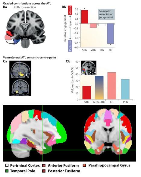
We now mention this area of overlap in our manuscript and link it to the hub and spokes model:
“Notably, our perirhinal cortex mask overlaps with a key region of the ventral anterior temporal lobe thought to be the central locus of crossmodal integration in the “hub and spokes” model of semantic representations.9,50 – pg. 20
(D) While most effects seem robust from the information presented, I'm not so sure about the analysis of the perirhinal cortex shown in Figure 5. This compares (I think) the neural similarity evoked by a unimodal stimulus ("feature") to that evoked by the same stimulus when paired with its congruent stimulus in the other modality ("object"). These similarities show an interaction with modality prior to cross-modal association, but no interaction afterward, leading the authors to suggest that the perirhinal cortex has become less biased toward visual structure following learning. But the plots in Figures 4a and b are shown against different scales on the y-axes, obscuring the fact that all of the similarities are smaller in the after-learning comparison. Since the perirhinal interaction was already the smallest effect in the pre-learning analysis, it isn't really surprising that it drops below significance when all the effects diminish in the second comparison. A more rigorous test would assess the reliability of the interaction of comparison (pre- or post-learning) with modality. The possibility that perirhinal representations become less "visual" following cross-modal learning is potentially important so a post hoc contrast of that kind would be helpful.
We apologize for the lack of clarity. We conducted a linear mixed model to assess the interaction between modality and crossmodal learning day (before and after crossmodal learning) in the perirhinal cortex as described by the reviewer. The critical interaction was significant, which is now clarified in the text as well as in the rescaled figure plots.
“To investigate this effect in perirhinal cortex more specifically, we conducted a linear mixed model to directly compare the change in the visual bias of perirhinal representations from before crossmodal learning to after crossmodal learning (green regions in Figure 5a vs. 5b). Specifically, the linear mixed model included learning day (before vs. after crossmodal learning) and modality (visual feature match to crossmodal object vs. sound feature match to crossmodal object). Results revealed a significant interaction between learning day and modality in the perirhinal cortex (F1,775 = 5.56, p = 0.019, η2 = 0.071), meaning that the baseline visual shape bias observed in perirhinal cortex (green region of Figure 5a) was significantly attenuated with experience (green region of Figure 5b). After crossmodal learning, a given shape no longer invoked significant pattern similarity between objects that had the same shape but differed in terms of what they sounded like. Taken together, these results suggest that prior to learning the crossmodal objects, the perirhinal cortex had a default bias toward representing the visual shape information and was not representing sound information of the crossmodal objects. After crossmodal learning, however, the visual shape bias in perirhinal cortex was no longer present. That is, with crossmodal learning, the representations within perirhinal cortex started to look less like the visual features that comprised the crossmodal objects, providing evidence that the perirhinal representations were no longer predominantly grounded in the visual modality.” – pg. 13
We note that not all effects drop in Figure 5b (even in regions with a similar numerical pattern similarity to PRC, like the hippocampus – also see Supplemental Figure S5 for a comparison for patterns only on Day 4), suggesting that the change in visual bias in PRC is not simply due to noise.
“Importantly, the change in pattern similarity in the perirhinal cortex across learning days (Figure 5) is unlikely to be driven by noise, poor alignment of patterns across sessions, or generally reduced responses. Other regions with numerically similar pattern similarity to perirhinal cortex did not change across learning days (e.g., visual features x crossmodal objects in A1 in Figure 5; the exploratory ROI hippocampus with numerically similar pattern similarity to perirhinal cortex also did not change in Supplemental Figure S4c-d).” – pg. 14
(E) Is there a reason the authors did not look at representation and change in the hippocampus? As a rapid-learning, widely-connected feature-binding mechanism, and given the fairly minimal amount of learning experience, it seems like the hippocampus would be a key area of potential import for the cross-modal association. It also looks as though the hippocampus is implicated in the localizer scan (Figure 3c).
We thank the reviewer for this suggestion and now include additional analyses for the hippocampus. We found no evidence of crossmodal integrative coding different from the unimodal features. Rather, the hippocampus seems to represent the convergence of unimodal features, as evidenced by …[can you give some pithy description for what is meant by “convergence” vs “integration”?]. We provide these results in the Supplemental Information and describe them in the main text:
“Analyses for the hippocampus (HPC) and inferior parietal lobe (IPL). (a) In the visual vs. auditory univariate analysis, there was no visual or sound bias in HPC, but there was a bias towards sounds that increased numerically after crossmodal learning in the IPL. (b) Pattern similarity analyses between unimodal features associated with congruent objects and incongruent objects. Similar to Supplemental Figure S3, there was no main effect of congruency in either region. (c) When we looked at the pattern similarity between Unimodal Feature runs on Day 2 to Crossmodal Object runs on Day 2, we found that there was significant pattern similarity when there was a match between the unimodal feature and the crossmodal object (e.g., pattern similarity > 0). This pattern of results held when (d) correlating the Unimodal Feature runs on Day 2 to Crossmodal Object runs on Day 4, and (e) correlating the Unimodal Feature runs on Day 4 to Crossmodal Object runs on Day 4. Finally, (f) there was no significant pattern similarity between Crossmodal Object runs before learning correlated to Crossmodal Object after learning in HPC, but there was significant pattern similarity in IPL (p < 0.001). Taken together, these results suggest that both HPC and IPL are sensitive to visual and sound content, as the (c, d, e) unimodal feature-level representations were correlated to the crossmodal object representations irrespective of learning day. However, there was no difference between congruent and incongruent pairings in any analysis, suggesting that HPC and IPL did not represent crossmodal objects differently from the component unimodal features. For these reasons, HPC and IPL may represent the convergence of unimodal feature representations (i.e., because HPC and IPL were sensitive to both visual and sound features), but our results do not seem to support these regions in forming crossmodal integrative coding distinct from the unimodal features (i.e., because representations in HPC and IPL did not differentiate the congruent and incongruent conditions and did not change with experience). * p < 0.05, ** p < 0.01, *** p < 0.001. Asterisks above or below bars indicate a significant difference from zero. Horizontal lines within brain regions in (a) reflect an interaction between modality and learning day, whereas horizontal lines within brain regions in reflect main effects of (b) learning day, (c-e) modality, or (f) congruency.” – Supplemental Figure S4.
“Notably, our perirhinal cortex mask overlaps with a key region of the ventral anterior temporal lobe thought to be the central locus of crossmodal integration in the “hub and spokes” model of semantic representations.9,50 However, additional work has also linked other brain regions to the convergence of unimodal representations, such as the hippocampus51,52,53 and inferior parietal lobes.54,55 This past work on the hippocampus and inferior parietal lobe does not necessarily address the crossmodal binding problem that was the main focus of our present study, as previous findings often do not differentiate between crossmodal integrative coding and the convergence of unimodal feature representations per se. Furthermore, previous studies in the literature typically do not control for stimulus-based factors such as experience with unimodal features, subjective similarity, or feature identity that may complicate the interpretation of results when determining regions important for crossmodal integration. Indeed, we found evidence consistent with the convergence of unimodal feature-based representations in both the hippocampus and inferior parietal lobes (Supplemental Figure S4), but no evidence of crossmodal integrative coding different from the unimodal features. The hippocampus and inferior parietal lobes were both sensitive to visual and sound features before and after crossmodal learning (see Supplemental Figure S4c-e). Yet the hippocampus and inferior parietal lobes did not differentiate between the congruent and incongruent conditions or change with experience (see Supplemental Figure S4).” – pg. 20
(F) The direction of the neural effects was difficult to track and understand. I think the key observation is that TP and PRh both show changes related to cross-modal congruency - but still it would be helpful if the authors could articulate, perhaps via a schematic illustration, how they think representations in each key area are changing with the cross-modal association. Why does the temporal pole come to activate less for congruent than incongruent stimuli (Figure 3)? And why do TP responses grow less similar to one another for congruent relative to incongruent stimuli after learning (Figure 4)? Why are incongruent stimulus similarities anticorrelated in their perirhinal responses following cross-modal learning (Figure 6)?
We thank the author for identifying this issue, which was also raised by the other reviewers. The reviewer is correct that the key observation is that the TP and PRC both show changes related to crossmodal congruency (given that the unimodal features were equated in the methodological design). However, the structure of the integrative code is less clear, which we now emphasize in the main text. Our findings provide evidence of a crossmodal integrative code that is different from the unimodal features, and future studies are needed to better understand the structure of how such a code might emerge. We now more clearly highlight this distinction throughout the paper:
“By contrast, perirhinal cortex may be involved in pattern separation following crossmodal experience. In our task, participants had to differentiate congruent and incongruent objects constructed from the same three shape and sound features (Figure 2). An efficient way to solve this task would be to form distinct object-level outputs from the overlapping unimodal feature-level inputs such that congruent objects are made to be orthogonal from the representations before learning (i.e., measured as pattern similarity equal to 0 in the perirhinal cortex; Figure 5b, 6, Supplemental Figure S5), whereas non-learned incongruent objects could be made to be dissimilar from the representations before learning (i.e., anticorrelation, measured as patten similarity less than 0 in the perirhinal cortex; Figure 6). Because our paradigm could decouple neural responses to the learned object representations (on Day 4) from the original component unimodal features at baseline (on Day 2), these results could be taken as evidence of pattern separation in the human perirhinal cortex.11,12 However, our pattern of results could also be explained by other types of crossmodal integrative coding. For example, incongruent object representations may be less stable than congruent object representations, such that incongruent objects representation are warped to a greater extent than congruent objects (Figure 6).” – pg. 18
“As one solution to the crossmodal binding problem, we suggest that the temporal pole and perirhinal cortex form unique crossmodal object representations that are different from the distributed features in sensory cortex (Figure 4, 5, 6, Supplemental Figure S5). However, the nature by which the integrative code is structured and formed in the temporal pole and perirhinal cortex following crossmodal experience – such as through transformations, warping, or other factors – is an open question and an important area for future investigation. Furthermore, these anterior temporal lobe structures may be involved with integrative coding in different ways. For example, the crossmodal object representations measured after learning were found to be related to the component unimodal feature representations measured before learning in the temporal pole but not the perirhinal cortex (Figure 5, 6, Supplemental Figure S5). Moreover, pattern similarity for congruent shape-sound pairs were lower than the pattern similarity for incongruent shape-sound pairs after crossmodal learning in the temporal pole but not the perirhinal cortex (Figure 4b, Supplemental Figure S3a). As one interpretation of this pattern of results, the temporal pole may represent new crossmodal objects by combining previously learned knowledge. 8,9,10,11,13,14,15,33 Specifically, research into conceptual combination has linked the anterior temporal lobes to compound object concepts such as “hummingbird”.34,35,36 For example, participants during our task may have represented the sound-based “humming” concept and visually-based “bird” concept on Day 1, forming the crossmodal “hummingbird” concept on Day 3; Figure 1, 2, which may recruit less activity in temporal pole than an incongruent pairing such as “barking-frog”. For these reasons, the temporal pole may form a crossmodal object code based on pre-existing knowledge, resulting in reduced neural activity (Figure 3d) and pattern similarity towards features associated with learned objects (Figure 4b).” – pg. 18
This work represents a key step in our advancing understanding of object representations in the brain. The experimental design provides a useful template for studying neural change related to the cross-modal association that may prove useful to others in the field. Given the broad variety of open questions and potential alternative analyses, an open dataset from this study would also likely be a considerable contribution to the field.
Author Response
Reviewer #3 (Public Review):
Gavanetto et al. propose an interesting method to identify membrane proteins based on the analysis of single-molecule AFM (smAFM) force-extension traces obtained from native plasma membranes. In the proposed pipeline, the authors use smAFM to non-specifically probe isolated plasma membranes by recording a large number (millions) of force-extension traces. While, as expected, most of them lack any binding or represent spurious events, the authors use an unsupervised clustering algorithm to identify groups of force-extension curves with a similar mechanical pattern, suggesting that each cluster corresponds to a unique protein species that can be fingerprinted by its specific force-extension pattern. By implementing a Bayesian framework, the authors contrast the identified groups with proteomics databases, which provide the most likely proteins that correspond to the identified force-extension clusters. A set of control experiments complements the manuscript to validate the proposed methodology, such as the application of their pipeline using purified samples or overexpressing a specific protein species to enrich its population.
The primary strength of the manuscript is its originality, as it proposes a novel application of smAFM as a protein-detection method that can be applied in native samples. This methodology combines ingredients from conventional mass spectrometry and cryoEM; the contour length released upon extending a protein is a direct measure of its sequence extension (related to its mass), but the force pattern contains insightful information about the protein's structure. In this sense, the authors' proposal is very smart. However, the relationship between protein structure and mechanics is far from straightforward, and here perhaps lies one of the main limitations of the proposed method. This is particularly true for the case of membrane proteins, where we cannot talk about protein unfolding in its classical sense but rather about pullout events which is likely what each peak corresponds to (indeed, the authors speak throughout the paper about unfolding events, which I believe is not the correct term).
We fully agree with the semantics concern of reviewer #3 about the term unfolding. A membrane protein when pulled with the tip of the AFM is pulled out of the membrane (see 2 in the image below) and, simultaneously, the segment that is pulled out unfolds (see 3). To our knowledge, force peaks corresponding to a contour length equal to 2 where not consistently observed or reported (when e.g. a transmembrane alpha helix is out of the membrane but folded).
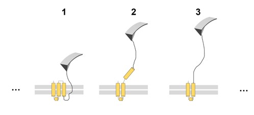
Since the field evolved with the practice of using the term ‘unfolding’ even for membrane proteins (see for instance (Kessler and Gaub, 2006; Oesterhelt et al., 2000; Yu et al., 2017) and many others), we would prefer to stick with this term.
In the context of membrane proteins the term unfolding therefore refers to at least the tertiary structure of the protein, because it is not clear when and at which timescale the secondary structures really unfolds.
We pointed this out in Line 131 (and following Lines).
Author Response
Reviewer #1 (Public Review):
This is a well performed study to demonstrate the antiviral function and viral antagonism of the dynein activating adapter NINL. The results are clearly presented to support the conclusions.
This reviewer has only one minor suggestion to improve the manuscript.
Add a discussion (1) why the folds of reduction among VSV, SinV and CVB3 were different in the NINL KO cells and (2) why the folds of reduction of VSV in the NINL KO A549 and U-2 OS cells.
Thank you for this suggestion. We have amended the results section to include additional information about these observations and possible explanations for these results.
Reviewer #2 (Public Review):
This manuscript is of interest to readers for host-viral co-evolution. This study has identified a novel human-virus interaction point NINL-viral 3C protease, where NINL is actively evolving upon the selection pressure against viral infect and viral 3Cpro cleavage. This study demonstrates that the viral 3Cpros-mediated cleavage of host NINL disrupts its adaptor function in dynein motor-mediated cargo transportation to the centrosome, and this disruption is both host- and virus-specific. In addition, this paper indicates the role of NINL in the IFN signaling pathway. Data shown in this manuscript support the major claims.
In this paper, the authors have identified a novel host-viral interaction, where viral 3C proteases (3Cpro) cleave at specific sites on a host activating adaptor of dynein intracellular transportation machinery, ninein-like protein (NINL or NLP in short) and inhibit its role in the antiviral innate immune response.
The authors firstly found that, unlike other activating adaptors of dynein intracellular transportation machinery, NINL (or NLP) is rapidly evolving. Thus, the authors hypothesized that this rapid evolution of NINL was caused by its interaction with viral infection. The authors found that viruses replicated higher in NINL knock-out (KO) cells than in wild-type (WT) cells and the replication level was not attenuated upon IFNa treatment in NINL KO cells, unlike in WT cells. Next, the authors investigated the role of NINL in type I IFN-mediated immune response and found that the induction of Janus kinase/signal transducer and activation of transcription (JAK/STAT) genes were attenuated in NINL KO cells upon IFNa treatment. The author further showed that the reduction of replication IFNa sensitive Vaccinia virus mutant upon IFNa treatment was decreased in NINL KO A549 cells compared to WT cells. The authors further showed that the virus antagonized NINL function by cleaving it with viral 3Cpro at its specific cleavage sites. NINL-peroxisome ligation-based cargo trafficking visualization assay showed that the redistribution of immobile membrane-bound peroxisome was disrupted by cleavage of NINL or viral infection.
This paper has revealed a novel host-virus interaction, and an antiviral function of a rapidly evolving activating adaptor of dynein intracellular transportation machinery, NINL. The major conclusions of this paper are well supported by data, but several aspects can be improved.
1) It would be necessary to include a couple of other pathways involved in innate immune response besides JAK/STAT pathway.
We are very interested in this question as well. Our RNAseq data (Supplementary file 4 and Figure 3 – Figure supplement 4) suggest that there are several transcriptional changes that result from NINL KO. Our goal in this manuscript was to focus on IFN signaling in order to understand this specific effect of NINL KO since it might have wide-ranging consequences on viral replication. While we agree that broadening our studies to other signaling pathways, including other pathways involved in innate immune response, is a good idea, we feel that those experiments would take longer than two months to perform and therefore fall outside of the scope of this paper.
2) The in-cell cleavages of NINL by viral 3Cpros were well demonstrated and supported by data of high quality. A direct biochemical demonstration of the cleavage is needed with purified proteins.
We agree with the reviewer that a direct biochemical cleavage assay would further demonstrate that viral 3Cpros cleave NINL specifically. However, our attempts to purify full-length NINL have been unsuccessful due to solubility issues (see example gel below), which is not surprising given that NINL is a >150 kDa human protein that has multiple surfaces that bind to other human proteins. As such, we focused our efforts on in-cell cleavage assays using specificity controls for cleavage. Specifically, we used catalytically inactive CVB3 3Cpro to show a dependence on protease catalytic activity and a variety of NINL constructs in which the glutamine in the P1 position is replaced by an arginine to show site specificity of cleavage. Notably, the cleavage sites in NINL that we mapped using this mutagenesis were predicted bioinformatically from known sites of 3Cpro cleavage in viral polyproteins, further indicating that cleavage is 3Cpro-dependent. We believe these results thus demonstrate that cleavage of NINL is dependent on viral protease activity and occurs in a sequence-specific manner. In light of the difficulty of purifying full-length NINL that would make biochemical experiments very challenging and likely take longer than two months to perform, we believe that our in cell data should be sufficient to demonstrate activity-dependent site-specific cleavage of NINL by viral 3Cpros.
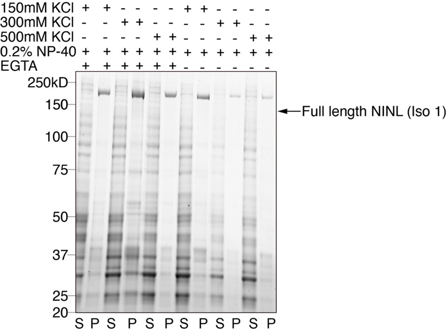
Sypro stained SDS-PAGE gel showing supernatant (S) and insoluble pellet (P) fractions across multiple purifications with altered buffer conditions.
3) The author used different cell types in different assays. Explain the rationale with a sentence for each assay.
Throughout this work, we choose to use a variety of cell lines for specific purposes. A549 cells were chosen as our main cell line as they are widely used in virology, are susceptible to the viruses we used, are responsive to interferon, and express both NINL and our control NIN at moderate levels. In the case of our virology and ISG expression data, we performed the same experiments with NINL KOs in other cell lines confirm that the phenotypes we observed in A549 cells could be attributed to the absence of NINL rather than off-target CRISPR perturbations or cell-line specific effects. All cleavage experiments were performed in HEK293T for their ease of transfection and protein expression. The inducible peroxisome trafficking assays were performed in U-2 OS cells as their morphology is ideal for observing the spatial organization of peroxisomes via confocal microscopy, and based on the fact that we had recapitulated the virology results and ISG expression results in those cells. At the suggestion of the reviewer, we have amended the text to include rationales where appropriate.
4) While cell-based assays well support the conclusions in this paper, further demonstration in vivo would be helpful to provide an implication on the pathogenicity impact of NINL.
We agree. However, we believe that examining the impact of the loss of or antagonism of NINL on the pathogenesis of infectious diseases in an in vivo model is outside the scope of this study.
In summary, this manuscript contributes to a novel antiviral target. In addition, it is important to understand the host-virus co-evolution. The use of the evolution signatures to identify the "conflict point" between host and virus is novel.
Author Response:
Reviewer #1:
In this manuscript Hill et al, analyze immune responses to vaccination of adults with the seasonal influenza vaccine. They perform a detailed analysis of the hemagglutinin-specific binding antibody responses against several different strains of influenza, and antigen-specific CD4+ T cells/T follicular cells, and cytokines in the plasma. Their analysis reveals that: (i) tetramer positive, HA-specific T follicular cells induced 7 days post vaccination correlate with the binding Ab response measured 42 days later; (ii) the HA-specific T fh have a diverse TCR repertoire; (iii) Impaired differentiation of HA-specific T fh in the elderly; and (iv) identification of an "inflammatory" gene signature within T fh in the elderly, which is associated with the impaired development of HA-specific Tfh.
The paper addresses a topic of considerable interest in the fields of human immunology and vaccinology. In general the experiments appear well performed, and support the conclusions. However, the following points should be addressed to enhance the clarity of the paper, and add support to the key conclusions drawn.
We thank the reviewer for their supportive evaluation of the manuscript, and have provided the details of how we have addressed each the points raised below.
1) Abstract: "(cTfh) cells are the best predictor of high titre antibody responses.." Since the authors have not done any blind prediction using machine learning tools with independent cohort, the sentence should be rephrased thus: "cTfh) cells are were associated with high titre antibody responses."
We agree that this phrasing better reflects the presented data. The sentence in the abstract (page 2) now reads “we show that formation of circulating T follicular helper (cTfh) cells was associated with high titre antibody responses.”
2) Figure 1A: Please indicate the age range of the subjects.
Figure 1 has been updated to include the age range of the subjects.

3) Almost all the data in the paper shows binding Ab titers. Yet, typically HAI titers of MN titers are used to assess Ab responses to influenza. Fig 1C shows HAI titers against the H1N1 Cal 09 strain. Can the authors show HAI titers for Cal 09 and the other A and B strains contained in the 2 vaccine cohorts? Do such HAI titers correlate with the tetramer positive cells, similar to the correlations show in Fig 2e.
In this manuscript we have deliberately focussed on the immune response to the H1N1 Cal09 strain, as it is the only influenza strain in the vaccine common to both cohorts. The HAI titre for this strain is now shown as supplementary figure 4. In addition, the class II tetramers were specifically selected to recognise unique epitopes in the Cal 09 strain (J. Yang, {..} W. W. Kwok, CD4+ T cells recognize unique and conserved 2009 H1N1 influenza hemagglutinin epitopes after natural infection and vaccination. Int Immunol 25, 447-457, 2013) because of this we do not think it is appropriate to correlate HAI titres for the non-Cal 09 strains with tetramer positive cells. We agree that showing the correlation of cTfh and other immune parameters with the HAI titres for Cal 09 is important and have included this as supplementary figure 7. The new data and text are presented below:

Figure 1-figure supplement 4: HAI responses before and after vaccination A) Log2 HAI titres at baseline (d0), d7 and d42 for cohort 1 (n=16) and B) cohort 2 (n = 21). C) Correlation between HAI and A.Cali09 IgG as measured by Luminex assay for cohort 1 and 2 combined. p-values determined using paired Wilcoxon signed rank-test, and Pearson’s correlation.
Text changes. Page 4. “The increase in anti-HA antibody titre was coupled with an increase in hemagglutination inhibitory antibodies to A.Cali09, the one influenza A strain contained in the TIVs that was shared across the two cohorts and showed a positive correlation with the A.Cali09 IgG titres measured by Luminex assay (Fig. 1C, Figure 1-figure supplement 4).”

Figure 2-figure supplement 1: Correlations between HAI assay titres and selected immune parameters. Correlation between vaccine-induced A.Cali09 HAI titres at d42 with selected immune parameters in both Cohort 1 and Cohort 2 (n=37). Dot color corresponds to the cohort (black = Cohort 1, grey = Cohort 2). Coefficient (Rho) and p-value determined using Spearman’s correlation, and line represents linear regression fit.
Results text Changes: Page 5. “Similar trends were seen when these immune parameters were correlated to HAI titres against A/Cali09 (Fig Figure 2-figure supplement 1).”
4) Fig 2d to i: what % of all bulk activated Tfh at day 7 are tetramer positive? The tetramer positive T cells constitute roughly 0.094% of all CD4 T cells (Fig 2d), of which 1/3rd are CXCR5+, PD1+ (i.e. ~0.03% of CD4 T cells). What fraction of all activated Tfh is this subset of tetramer positive cells? Presumably, there will also be Tfh generated against other viral proteins in the vaccine, and these will constitute a significant fraction of all activated Tfh.
This is an important point, as the tetramers only recognise one peptide epitope of the Cal.09 HA protein, so there will be many other influenza reactive CD4+ T cells that are responding to other Cal 09 epitopes as well as other proteins in the vaccine. The analysis suggested by the reviewer shows that the frequency of Tet+ cells amongst bulk cTfh cells ranges from 0.14%-1.52% in cohort 1, and from 0.022-2.7% in cohort 2. These data have been included as Figure Figure 1-figure supplement 6C, D in the revised manuscript. In addition, Tet+ cells as a percentage of bulk cTfh cells were reduced in older people compared to younger adults. This data has been included in Figure 5-figure supplement 1C in the revised manuscript.

Figure 1-figure supplement 6: Percentage of cTfh cells that are Tet+ and CXCR3 and CCR6 expression on HA-specific CD4+ T cells. A) Representative flow cytometry gating strategy for CXCR5+PD-1+ cTfh cells on CD4+CD45RA- T cells, and the proportion of HA-specific Tet+ cells within the CXCR5+PD-1+ cTfh cell gate. B) Percentage Tet+ cells within the CXCR5+PD-1+ cTfh cell population. Within-cohort age group differences were determined using the Mann-Whitney U test.
Results text, page 4: These antigen-specific T cells had upregulated ICOS after immunisation, indicating that they have been activated by vaccination (Fig. 1F, G). In addition, a median of one third of HA-specific T cells upregulated the Tfh markers CXCR5 and PD1 on d7 after immunisation (Fig. 1H, I). The tetramer binding cells represented between 0.022-2.7% of the total CXCR5+PD-1+ bulk population (Fig Figure 1-figure supplement 6A, B).

Figure 5-figure supplement 1C: Age-related differences in cytokines and HA-specific CD4+ T cell parameters. C) Percentage Tet+ cells within the CXCR5+PD-1+ cTfh cell population. Within-cohort age group differences were determined using the Mann-Whitney U test.
Results text, page 8: Across both cohorts, the only CD4+ T cell parameters consistently reduced in older individuals at d7 were the frequency of polyclonal cTfh cells and HA-specific Tet+ cTfh cells, with the strongest effect within the antigen-specific cTfh cell compartment (Fig. 5H-J, Figure 5-figure supplement 1C).
Reviewer #2:
Hill and colleagues present a comprehensive dataset describing the recall and expansion of HA-specific cTFH cells following influenza immunisation in two cohorts. Using class II tetramers, IgG titres against a large panel of HA antigens, and quantification of plasma cytokines, they find that activated and HA-specific cTFH cells were a strong predictor of the IgG response against the vaccine after 6 weeks. Using RNAseq and TCR clonotype analysis, they find that, in 10/15 individuals, the HA-specific cTFH response at day 7 post-vaccination is recalled from the available CD4 T cell memory pool present prior to vaccination. Post-vaccination HA-specific cTFH cells exhibited a transcriptional profile consistent with lymph node-derived GC TFH, as well as evidence of downregulation of IL-2 signaling pathways relative to pre-vaccine CD4 memory cells.
The authors then apply these findings to a comparison of vaccine immunogenicity between younger (18-36) and older (>65) adults. As expected, they found lower levels of vaccine-specific IgG responses among the older cohort. Analysis of HA-specific T cell responses indicated that tet+ cTFH fail to properly develop in the older cohort following vaccination. Further analysis suggests that development of HA-specific cTFH in older individuals is not caused by a lack of TCR diversity, but is associated with higher expression of inflammation-associated transcripts in tet+ cTFH.
Overall this is an impressive study that provides clarity around the recall of HA-specific CD4 T cell memory, and the burst of HA-specific cTFH cells observed 7 days post-vaccination. The association between defective cTFH recall and lower IgG titres post-vaccination in older individuals provides new targets for improving influenza vaccine efficacy in this age group. However, as currently presented, the model of impaired cTFH differentiation in the older cohort and the link to inflammation is somewhat unclear. There are several issues that could be clarified to improve the manuscript in its current form:
We thank the reviewer for their supportive and comprehensive summary of our work. We agree that the link between impaired inflammation and cTfh differentiation is correlative, we have added new data to address this, including mechanistic data to support chronic IL-2 signalling as antagonistic to cTfh development, as well as providing new analyses to address the other points raised.
1) It is somewhat unclear the extent to which the reduction in HA-specific cTFH in the older cohort is also related to an overall reduction in T cell expansion - cohort 1 shows a significant reduction in total tet+ CD4 T cells post-vaccination as well as in the cTFH compartment, and while this difference may not reach statistical significance, a similar trend is shown for cohort 2.
We agree that a possible interpretation is a global failure in T cell expansion in the older individuals. To determine whether there is a relationship between the degree of Tet+ CD4+ T cell expansion and cTfh cell differentiation with age, we performed correlation analyses. There is no correlation between the expansion of Tet+ cells and the frequency of cTfh cells formed seven days after immunisation in either age group. This suggests that the impaired cTfh cell differentiation in older persons is most likely caused by factors other than the capacity of CD4+ T cells to expand after vaccination. These data have been added as Figure 5-figure supplement 1D, and included in the results text on page 8.

Figure 5-figure supplement 1D: Age-related differences in cytokines and HA-specific CD4+ T cell parameters. D) Correlation between Tet+ cells (d7-d0, % of CD4+) and cTfh (d7-d0, % of TET+) in both cohorts for each age-group (18- 36 y.o n=37, 65+ y.o. n= 39). Dot color corresponds to the cohort (black = Cohort 1, grey = Cohort 2). Coefficient (Rho) and p-value determined using Spearman’s correlation, and line represents linear regression fit.
Text changes, Page 8: There was no consistent difference in the total d7 Tet+ HA-specific T cell population with age for both cohorts (Fig. 5H) and we observed no age-related correlation between the ability of an individual to differentiate Tet+ cells into a cTfh cell and the overall expansion of Tet+ HA-specific T cell population (Figure 5-figure supplement 1D). Thus, our data suggests that the poor vaccine antibody responses in older individuals is impacted by impaired cTfh cell differentiation (Fig. 5J) rather than size of the vaccine-specific CD4+ T cell pool.
2) Transcriptomic analysis indicates that HA-specific cTFH in the older cohort show impaired downregulation of inflammation, TNF and IL-2-related signaling pathways. The authors therefore conclude that excess inflammation can limit the response to vaccination. In its current presentation, the data does not necessarily support this conclusion. While it is clear that downregulation of TNF and IL-2 signalling pathways occur during cTFH/TFH differentiation, there is no evidence presented to support the idea that (a) vaccination results in increased pro-inflammatory cytokine production in lymphoid organs in older individuals or that (b) these pro-inflammatory cytokines actively promote CXCR5-, rather than cTFH, differentiation of existing memory T cells.
We agree with the reviewer that the data presented in figure 7 are correlative, rather than causative. Unfortunately, we do not have access to secondary lymphoid tissues from younger and older people after vaccination to test point (a) above. In order to test the hypothesis that increased inflammatory cytokine production in lymphoid organs limits Tfh cell differentiation we have used Il2cre/+; Rosa26stop-flox-Il2/+ transgenic mice. In this mouse model, IL-2-dependent cre- recombinase activity facilitates the expression of low levels of IL-2 in cells that have previously expressed IL-2. This creates a scenario in which cells that physiologically express IL-2 cannot turn its expression off therefore increasing expression IL-2 after antigenic stimulation (mice reported in Whyte et al., bioRxiv, 2020, doi: https://doi.org/10.1101/2020.12.18.423431).
Twelve days after influenza A infection, Il2cre/+; Rosa26stop-flox-Il2/+ transgenic mice have fewer Tfh cells in the draining mediastinal lymph node and in the spleen (Fig. 8A-C), this is accompanied by a reduction in the magnitude of the GC B cell response (Fig. 8D-E). These data provide a proof of concept that sustained IL-2 production limit the formation of Tfh cells, consistent with the negative correlation of an IL-2 signalling gene signature and cTfh cell formation in humans (Figure 7). These new data support the conclusion that excess IL-2 signalling can limit the Tfh cell response. These data are presented in Figure 8, and are discussed on page 12 in the results, and pages 12-13 in the discussion.

Figure 8: Increased IL-2 production impairs Tfh cell formation and the germinal centre response. Assessment of the Tfh cell and germinal centre response in Il2cre/+; Rosa26stop-flox-Il2/+ transgenic mice that do not switch off IL-2 production, and Il2cre/+; Rosa26+/+ control mice 12 days after influenza A infection. Flow cytometric contour plots (A) and quantification of the percentage of CXCR5highPD-1highFoxp3-CD4+ Tfh cells in the mediastinal lymph node (B) and spleen (C). Flow cytometric contour plots (D) and quantification of the percentage of Bcl6+Ki67+B220+ germinal centre B cells in the mediastinal lymph node (E) and spleen (F). The height of the bars indicates the median, each symbol represents one mouse, data are pooled from two independent experiments. P-values calculated between genotype-groups by Mann Whitney U test.
Results text, page 12: Sustained IL-2 production inhibits Tfh cell frequency and the germinal centre response. To test the hypothesis that cytokine signalling needs to be curtailed to facilitate Tfh cell differentiation turned to a genetically modified mouse model in which cells that have initiated IL-2 production cannot switch it off, Il2cre/+; Rosa26stop-flox-Il2/+ mice (37). Twelve days after influenza infection Il2cre/+; Rosa26stop-flox-Il2/+ mice have fewer Tfh cells in the draining lymph node and spleen (Fig. 8A-C), which is associated with a reduced frequency of germinal center B cells (Fig. 8D-F). This provides a proof of concept that proinflammatory cytokine production needs to be limited to enable full Tfh cell differentiation in secondary lymphoid organs.
Discussion text, pages 12, 13: These enhanced inflammatory signatures associated with poor antibody titre in an independent cohort of influenza vaccinees. The dampening of Tfh cell formation by enhanced cytokine production was confirmed by the use of genetically modified mice where IL-2 production is restricted to the appropriate anatomical and cellular compartments, but once initiated cannot be inactivated. Together, this suggests that formation of antigen-specific Tfh cells is essential for high titre antibody responses, and that excessive inflammatory factors can contribute to poor cTfh cell responses.
Author Response
Reviewer #1 (Public Review):
In the article "Neuroendocrinology of the lung revealed by single cell RNA sequencing", Kuo et. al. described various aspects of pulmonary neuroendocrine cells (PNECs) including the scRNA-seq profile of one human lung carcinoid sample. Overall, although this manuscript does not have any specific storyline, it is informative and would be an asset for researchers exploring various new roles of PNECs.
Thank you for appreciating the significance of the data presented. Our storyline focuses on the newly uncovered molecular diversity of PNECs and the extraordinary repertoire of peptidergic signals they express and cell types these signals can directly target in (and outside) the lung, in mice and human, and in health and disease (human carcinoid tumor).
Major comments:
The major concern about the work is most results are preliminary, and at a descriptive level, conclusions or sub-conclusions are derived from scRNA-seq analysis only, lacking in-depth functional analysis and validation in other methods or systems. There are many open-end results that have been predicted by the authors based on their scRNA-seq data analysis without functional validation. In order to give them a constructive roadmap, it would be better to investigate literature and put them in a potential or probable hypothesis by citing the available literature. This should be done in each section of the result part. The paper lacks a main theme or specific biology question to address. In addition, the description about the human lung carcinoid by scRNA-seq is somehow disconnected from the main study line. Also, these results are derived from the study on only one single patient, lacking statistical power.
We agree that much of the data and analysis presented in the paper is descriptive and hypothesis-generating for PNECs, however we do not consider it preliminary. We focused on validating two key conclusions from the scRNA-seq analysis: PNECs are extraordinarily diverse molecularly (as validated by multiplex in situ hybridization and immunostaining) and they express many different combinations of peptidergic signals (and appear to package them in separate vesicles). From the lung expression profiles of the cognate receptors, we also predicted the direct lung targets of the dozens of new PNEC peptidergic signals we uncovered, and validated the cell target (PSN4, a recently identified subtype of pulmonary sensory neuron) of one of the newly identified PNEC signals (the classic hormone angiotensin) by confirming expression of the cognate receptor gene in PSN4 neurons that innervate PNECs and showing that the hormone can directly activate PSN4 neurons. The characterized human carcinoid provided evidence that during tumorigenesis, the amplified PNECs retain a memory (albeit imperfect) of the molecular subtype of PNEC from which they originated. As suggested by the Reviewer, we have provided more background in Results by adding additional citations from the literature to clarify the rationale for each analysis and what was known prior to the analysis. We feel that our paper provides a broad foundation for exploring the diversity and signaling functions of PNECs, and although each molecular type of PNEC and new PNEC peptidergic signal we uncovered and potential target cell in (and outside) the lung warrants follow up (as do the sensory and other properties of PNECs we inferred from their expression profiles), such studies will require the effort of many individuals in many labs studying both normal and disease physiology in mouse and human, and exploiting the data, hypotheses, approaches, and framework we provide.
Reviewer #2 (Public Review):
Pulmonary neuroendocrine cells (PNECs) are known to monitor oxygen levels in the airway and can serve as stem cells that repair the lung epithelium after injury. Due to their rarity, however, their functions are still poorly understood. To identify potential sensory functions of PNECs, the authors have used single-cell RNA-sequencing (scRNA-seq) to profile hundreds of mouse and human PNECs. They report that PNECs express over 40 distinct peptidergic genes, and over 150 distinct combinations of these genes can be detected. Receptors for these neuropeptides and peptide hormones are expressed in a wide range of lung cell types, suggesting that PNECs may have mechanical, thermal, acid, and oxygen sensory roles, among others. However, since some of these cognate receptors are not expressed in the lung, PNECs may also have systemic endocrine functions. Although these data are largely descriptive, the results represent a significant resource for understanding the potential roles of PNECs in normal biology as well as in pulmonary diseases and cancer and are likely to be relevant for understanding neuroendocrine cells in other tissue contexts.
However, there are several aspects of the data analysis that are unclear and require clarification, most notably the definition of a neuroendocrine cell (points #1 and #2 below).
1) Figure S1 shows the sorting strategy used for isolation of putative PNECs from Ascl1CreER/+; Rosa26ZsGreen/+ mice, and distinguishes neuroendocrine cells defined as ZsGreen+ EpCAM+ and "neural" cells defined as ZsGreen+ EpCAM-; the figure legend also refers to the ZsGreen+ EpCAM- cells as "control" cells. However, the table shown in panel D indicates that the NE population combines 112 ZsGreen+ EpCAM+ cells together with 64 ZsGreen+ EpCAM- cells to generate the 176 cells used for subsequent analyses. Why are these ZsGreen+ EpCAM- cells initially labeled as neural or control, but are then defined as neuroendocrine? If these do not express an epithelial marker, can they be rigorously considered as neuroendocrine?
As explained above in the response to Essential Revision point 1, we define pulmonary neuroendocrine cells (PNECs) throughout the paper by their transcriptomic clustering and signatures, which includes the dozens of newly identified PNEC markers as well as the few extant marker genes available before this study (listed in Table S2). The confusion here arises from the two previously known markers (Ascl1 lineage marker ZsGreen, EpCAM) we used for flow sorting to enrich for these rare cells for transcriptomic profiling (Fig. S1). Although most of the cells with PNEC transcriptomic profiles were from the ZsGreenhi EpCAMhi sorted population (as expected), some were from the ZsGreenhi EpCAMlo sorted population. The latter resulted from the high EpCAM gating threshold we used during flow sorting, which excluded some PNECs with intermediate levels of surface EpCAM. Indeed, nearly all PNECs (> 95%) expressed EpCAM by scRNAseq, and there was no difference in EpCAM transcript levels or transcriptomic clustering of PNECs that were from the ZsGreenhi EpCAMhi vs. ZsGreenhi EpCAMlo sorted populations, as we now show in the new panels (C', C'') added to Fig S1C. This point is now clarified in the legend to Fig. S1C, and it nicely demonstrates that transcriptomic profiling is a more robust method of identifying PNECs than flow sorting based on two classical markers.
2) Similarly, in the human scRNA-seq analysis, how were PNECs defined? The methods description states that these cells were identified by their expression of CALCA and ASCL1, but does not indicate whether they also expressed epithelial markers.
Human PNECs were identified in the single cell transcriptomic analysis by the same strategy described above for mouse PNECs: by their transcriptomic clustering and signatures, which includes the dozens of newly identified PNEC markers as well as the few extant marker genes available before this study (listed in Table S2). In addition to expression of classic and new markers, the human PNEC cluster defined by scRNA-seq indeed showed the expected expressed of epithelial markers (e.g, EPCAM, see dotplot below), like other epithelial cells.
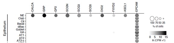
3) The presentation of sensitivity and specificity in Figure 1 is confusing and potentially misleading. According to Figure 1B, Psck1 and Nov are two of the top-ranked differentially expressed genes in PNECs with respect to both sensitivity and specificity. However, the specificity of these two genes appears to be lower than that of Scg5, Chgb, and several other genes, as suggested in Figure 1C and Figure S1E. In contrast, Chgb appears to have higher specificity and sensitivity than Psck1 in Figures 1C and E but is not shown in the list of markers in Figure 1B.
As explained above in the response to Essential Revision point 2, because different marker features are important for different applications, we have provided several different graphical formats (Figs. 1B,C, Fig. S1E) and a table (Table S1) to aid in selection of the optimal markers for each application. Fig. 1B shows the most sensitive and specific PNEC markers identified by ratio of the natural logs of the average expression of the marker in PNECs vs. non-PNEC epithelial cells (Table S1), and we have added a two-dimensional plot of this sensitivity and specificity for a large set of PNEC markers (new panel E of Fig. S1). The violin plots in Fig. 1C allow visual comparison of expression of selected markers across PNECs and 40 other lung cell types including non-epithelial cells (from our extensive mouse lung atlas in Travaglini, Nabhan et al, Nature 2020). Pcsk1 and Nov score high in the analysis of Fig. 1B because they are highly sensitive and specific markers within the pulmonary epithelium, and they are also valuable markers because they are highly expressed in PNECs. However, they appear slightly less specific in the violon plots of Fig. 1C (Pcsk1) and Fig. S1F (Nov) because of expression (though at much lower levels) in individual lung cell types outside the epithelium: Pcsk1 is expressed also at low levels in some Alox5+ lymphocytes, and Nov is expressed at low levels in some smooth muscle cells. Chgb is a new PNEC marker that did not make the cutoff for the list in Fig. 1B because it is expressed in a slightly higher percentage of non-PNEC epithelial cells than the markers shown, which ranked slightly above it by this metric (see Table S1).
4) The expression of serotonin biosynthetic genes in mouse versus human PNECs deserves some comment. The authors fail to detect the expression of Tph1 and Tph2 in any of the mouse PNECs analyzed, but TPH1 is expressed in 76% of the human PNECs (Table S8). Is it possible that Tph1 and Tph2 are not detected in the mouse scRNA-seq data due to gene drop-out? If serotonin signaling by mouse PNECs is due to protein reuptake, as implied on p. 5, is there a discrepancy between serotonin expression as detected by smFISH versus immunostaining?
It is always possible that the failure to detect expression of Tph1 and Tph2 in the mouse scRNA-seq dataset is due to technical dropout, however when we analyzed this in our other mouse PNEC scRNA-seq dataset obtained using a microfluidic platform and also deeply-sequenced (Ouadah et al, Cell 2019), we found similar values as in the previously analyzed dataset: no Tph2 expression was detected and only 3% (3 of 92) of PNECs had detected Tph1 expression, whereas 24% (22 of 92) had detected expression of serotonin re-uptake transporter Slc6a4. Because our mouse and human scRNA-seq datasets were prepared similarly and sequenced to a similar depth (105 to 106 reads/cell), the difference observed in Tph1/TPH1 expression between mouse (0-3% PNECs) and human (76% PNECs) is more likely a true biological difference. We also analyzed serotonin levels in mouse PNECs by immunohistochemistry (not shown) and detected serotonin in nearly all (~90%) embryonic PNECs but only ~10% of adult PNECs. Systematic follow up studies will be necessary to resolve the mechanism of serotonin biogenesis and uptake in PNECs, and the potential stage and species-specific differences in these processes suggested by this initial data.
5) The smFISH and immunostaining analyses are often presented without any indication of the number of independent replicate samples analyzed (e.g., Figure 2B, Figure 3F, G).
The number of samples analyzed have been added (the values for Fig. 2B are given in legend to Fig. 2C, the quantification of Fig. 2B).
6) It would be helpful to provide a statistical analysis of the similarities and differences shown in the graphs in Figures 1E and G.
We added a statistical analysis (Fisher's exact test, two-sided) of Fig. 1E comparing expression of each examined gene in the two scRNA-seq datasets (Table S4). We added a similar statistical analysis of Fig. 1G comparing the expression values of each examined gene by scRNA-seq vs smFISH (see Fig. 1G legend).
Author Responses
Reviewer #1 (Public Review):
This study uses a nice longitudinal dataset and performs relatively thorough methodological comparisons. I also appreciate the systematic literature review presented in the introduction. The discussion of confound control is interesting and it is great that a leave-one-site-out test was included. However, the prediction accuracy drops in these important leave-one-site-out analyses, which should be assessed and discussed further.
Furthermore, I think there is a missed opportunity to test longitudinal prediction using only pre-onset individuals to gain clearer causal insights. Please find specific comments below, approximately in order of importance.
We thank the reviewers for their positive remarks and for providing important suggestions to improve the analysis. Please see our detailed comments below.
1) The leave-one-site-out results fail to achieve significant prediction accuracy for any of the phenotypes. This reveals a lack of cross-site generalizability of all results in this work. The authors discuss that this variance could be caused by distributed sample sizes across sites resulting in uneven folds or site-specific variance. It should be possible to test these hypotheses by looking at the relative performance across CV folds. The site-specific variance hypothesis may be likely because for the other results confounds are addressed using oversampling (i.e., sampling with replacement) which creates a large sample with lower variance than a random sample of the same size. This is an important null finding that may have important implications, so I do not think that it is cause for rejection. However, it is a key element of this paper and I think it should be assessed further and discussed more widely in the abstract and conclusion.
We thank the reviewer for raising this point and providing specific suggestions. As mentioned by the reviewer, the leave-one-site-out results showed high-variance across sites, that is, across cross validation (CV) folds. Therefore, as suggested by the reviewer, we further investigated the source of this variance by observing how the model accuracies correlates with each site and its sample sizes, ratio of AAM-to-controls, and the sex distribution in each site. We ranked the sites from low to high accuracy and observed different performance metrics such as sensitivity and specificity:
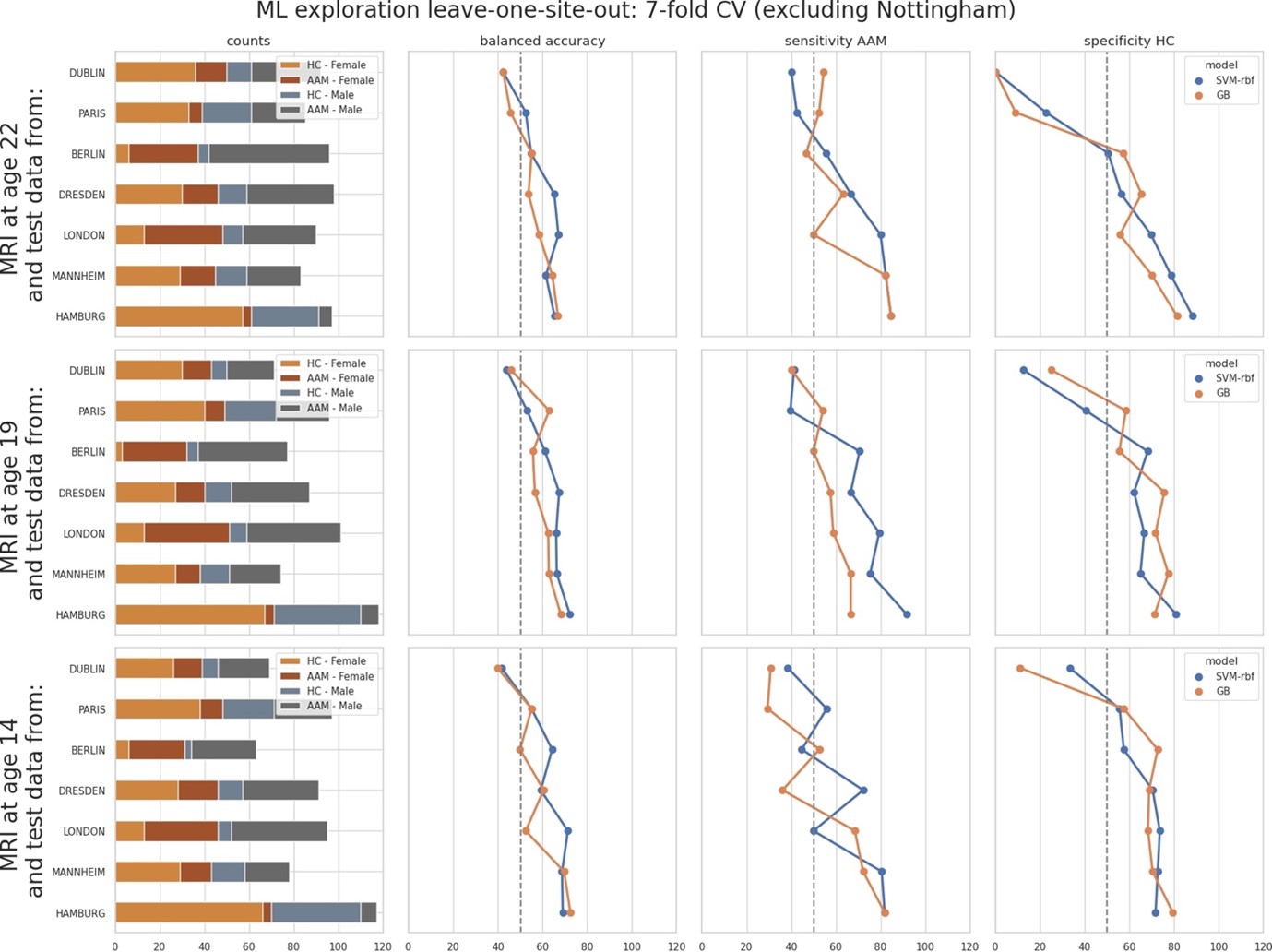
As shown, the models performed close-to-chance for sites ‘Dublin’, ‘Paris’ and ‘Berlin’ (<60% mean balanced accuracy) in the leave-one-site-out experiment, across all time-points and metrics. Notably, the order of the performance at each site does not correspond to the sample sizes (please refer to the ‘counts’ column in the above figure). It also does not correspond to the ratio of AAM-to-controls, or to the sex distribution.
To further investigate this, we performed another additional leave-one-site-out experiment with all 8 sites. Here, we repeated the ML (Machine Learning) exploration by using the entire data, including the data from the Nottingham site that was kept aside as the holdout. Since there are 8 sites now, we used a 8-fold cross validation and observed how the model accuracy varied across each site:
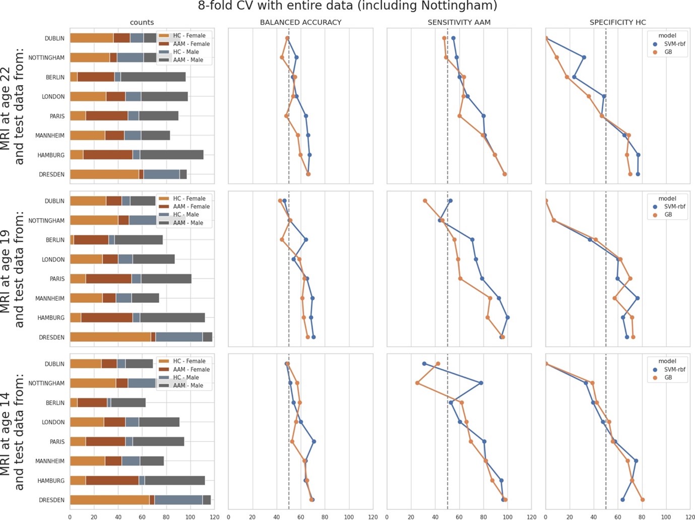
The results were comparable to the original leave-one-site-out experiment. Along with ‘Dublin’ and Berlin’, the models additionally performed poorly on the ‘Nottingham’ site. Results on ‘London’ and ‘Paris’ also fell below 60% mean balanced accuracy.
Finally, we compared the above two results to the main experiment from the paper where the test samples were randomly sampled across all sites. The performance on test subjects from each site was compared:
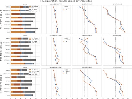
As seen, the models struggled with subjects from ‘Dublin’ followed by ‘Nottingham’ ‘London’ and ‘Berlin’ respectively, and performed well on subjects from ‘Dresden’, ‘Mannheim’, ‘Hamburg’ and ‘Paris’.
Across all the three results discussed above, the models consistently struggle to generalize to subjects particularly from ‘Dublin’ and ‘Nottingham’. As already pointed out by the reviewer, the variance in the main experiment in the manuscript is lower because of the random sampling of the test set across all sites. Since these results have important implications, we have included them in the manuscript and also provided these figures in the Appendix.
2) The authors state that "83.3% of subjects reported having no or just one binge drinking experience until age 14". To gain clearer insights into the causality, I recommend repeating the MRIage14 → AAMage22 prediction using only these 83% of subjects.
We thank the reviewer for this valuable comment. As suggested by the reviewer, we now repeated the MRIage14 → AAMage22 analysis by including (a) only the subjects who had no binge drinking experiences (n=477) by age 14 and (b) subjects who had one or less binge drinking experiences (n=565). The results are shown below. The balanced accuracy on the holdout set were 72.9 +/- 2% and 71.1 +/- 2.3% respectively, which is comparable to the main result of 73.1 +/- 2%.
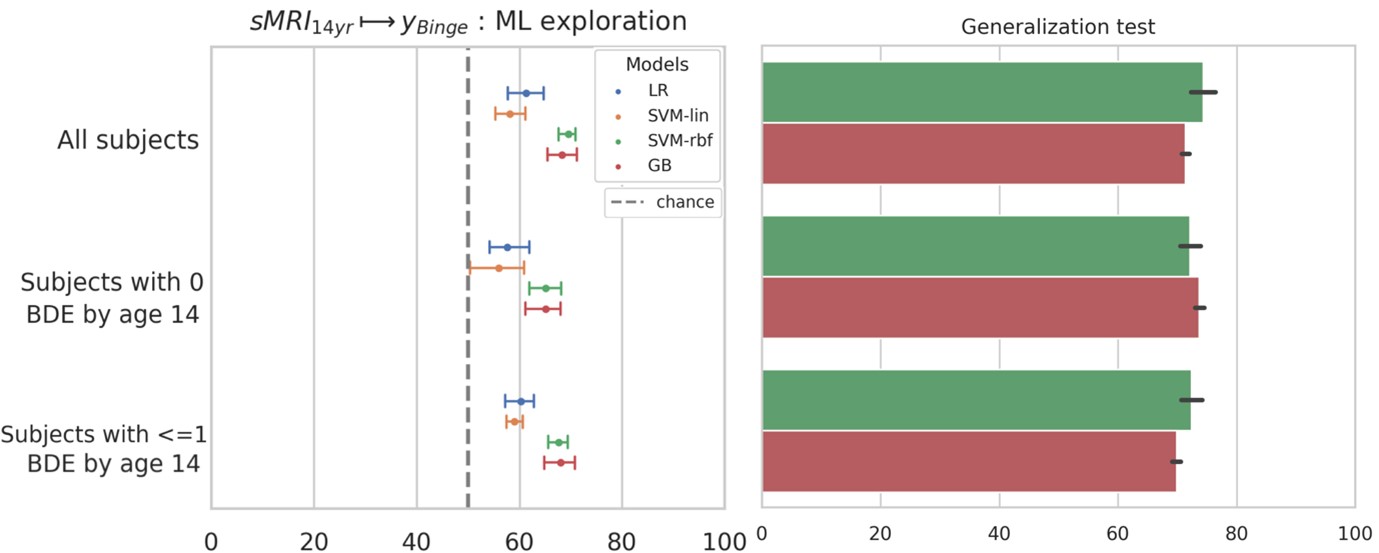
These results provide further evidence that certain form of cerebral predisposition might be preceding the observed alcohol misuse behavior in the IMAGEN dataset. We discuss these results now in the Results section and the 2nd paragraph of Discussion.
3) The feature importance results for brain regions are quite inconsistent across time points. As such, the study doesn't really address one of the main challenges with previous work discussed in the introduction: "brain regions reported were not consistent between these studies either and do not tell a coherent story". This would be worth looking into further, for example by looking at other indices of feature importance such as permutation-based measures and/or investigating the stability of feature importance across bootstrapped CV folds.
The feature importance results shown in Figure 9 is intended to be illustrative and show where the most informative structural features are mainly clustered around in the brain, for each time point. We would like to acknowledge that this figure could be a bit confusing. Hence, we have now provided an exhaustive table in the Appendix, consisting of all important features and their respective SHAP scores obtained across the seven repeated runs. In addition, we address the inconsistencies across time points in the 3rd paragraph in the Discussion chapter and contrast our findings with previous studies. These claims can now be verified from the table of features provided in the Appendix.
Addressing the reviewer's suggestions, we would like to point out that SHAP is itself a type of permutation-based measure of feature importance. Since it derives from the theoretically-sound shapley values, is model agnostic, and has been already applied for biomedical applications, we believe that running another permutation-based analysis would not be beneficial. We have also investigated the stability of our feature importance scores by repeating the SHAP estimation with different random permutations. This process is explained in the Methods section Model Interpretation.
Additionally now, the SHAP scores across the seven repetitions are also provided in the Appendix table 6 for verification.
Author Response
Reviewer #1 (Public Review):
This paper tests the hypothesis that 1/f exponent of LFP power spectrum reflects E-I balance in a rodent model and Parkinson's patients. The authors suggest that their findings fit with this hypothesis, but there are concerns about confirmation bias (elaborated on below) and potential methodological issues, despite the strength of incorporating data from both animal model and neurological patients.
First, the frequency band used to fit the 1/f exponent varies between experiments and analyses, inviting concerns about potentially cherry-picking the data to fit with the prior hypothesis. The frequency band used for fitting the exponent was 30-100 Hz in Experiment 1 (rodent model), 40-90 Hz in Experiment 2 (PD, levodopa), and 10-50 Hz in Experiment 3 (PD, DBS). Ad-hoc reasons were given to justify these choices, such as " to avoid a spectral plateau starting > 50 Hz" in Experiment 3. However, at least in Experiment 3 (Fig. 3), if the frequency range was shifted to 1-10 Hz, the authors would have uncovered the opposite effect, where the exponent is smaller for DBS-on condition.
We agree that parameter choice is crucial, in particular, choice of the fitting range. In addition to the 40-90 Hz range (Figure 2C), we have performed aperiodic fitting for five other frequency ranges to test to what extent the reported results are sensitive to the selected frequency range (Figure S2A). This analysis showed that the results are robust when a broad frequency range from 30 to 95 Hz was chosen, which is consistent with what has been suggested by Gao et al., 2017 to make inferences on the E/I ratio.
Accordingly, we have now repeated the analyses for the animal data with the same fitting range used for the ON-OFF medication comparison in humans. Along with Figure S2A where different frequency ranges were tested for data used in Figure 2, this shows that the results in Figure 1 and 2 hold up with higher aperiodic exponents when STN spiking is low and vice versa. Therefore, a broad fitting range from 30 to 90 Hz (excluding harmonics of mains interference) generates consistent results for both human and animal data.
We opted against a fitting range from 1-10 Hz because of two restraints highlighted in Gerster et al., 2022. First, a fitting range starting at 1 Hz could have a larger y-intercept due to the presence of low-frequency oscillations. This could lead to a larger aperiodic exponent and could be misinterpreted as stronger neural inhibition. Therefore, the lower fitting bound should be chosen to best avoid known oscillations in the delta/theta range (Gerster et al., 2022). Second, frequencies should be chosen to avoid oscillations crossing fitting range limits. In Figure 3A, oscillations in the theta/alpha band both ON and OFF stimulation would complicate parameterisation and would likely result in spurious fits.
We also tested the effect of changing the peak threshold, peak width limits and the aperiodic fitting mode on FOOOF parameterisation. Increasing and decreasing the peak threshold from its default value (at 2 standard deviations) did not change results (Figure S2B). Similarly, adapting the peak width limits did not affect the exponent difference between medication states (Figure S2C). Finally, choosing the ‘knee’ mode instead of ‘fixed’ resulted in fundamentally different aperiodic fits that did not differ anymore with medication (Figure S2D). This is most likely a consequence of the near linear PSD in log-log space from 40 to 90 Hz (Figure 2B). If there is no bend in the PSD, the FOOOF algorithm will be forced to assign a ‘random’ knee and the aperiodic fit will then mostly reflect the slope of the spectrum above the knee point.
Second, there are important, fine-grained features in the spectra that are ignored in the analyses, which confounds the interpretation.
One salient example of this is Fig. 2, where based on the plots in B, one would expect that the power of beta-band oscillations to be higher in the Med-On condition, as the oscillatory peaks rise higher above the 1/f floor and reach the same amplitude level as the Med-OFF condition (in other words, similar total power is subtracted by a smaller 1/f power in the Med-ON condition). But this impression is opposite to the model-fitting results in C, where beta power is lower in the Med-ON condition.
We agree that PSDs over a broad frequency range (e.g. 5-90 Hz) typically do not have a single 1/f property. Instead, there can be multiple oscillatory peaks and ‘knees/bends’ in the aperiodic component. For these cases, fitting should be performed using the knee mode. To extract periodic beta power, we parameterise the PSD between 5 and 90 Hz and select the largest oscillatory component between 8 and 35 Hz (this range was extended to include the large oscillatory peaks in hemispheres 27 and 28 at ~ 10 Hz, see Figure R1). We now use the knee mode, to model the aperiodic component between 5 and 90 Hz when periodic beta power is calculated (see our previous comments). Figure R1 provides an overview of all PSDs ON and OFF medication, the aperiodic fits (5-90 Hz (knee) and 40-90 Hz (fixed)) and the detected beta peaks. In spite of this modification in our pipeline, periodic beta power is still larger OFF medication (Figure 2C), in keeping with previous studies (Kim et al., 2022; Kühn et al., 2006; Neumann et al., 2017; Ray et al., 2008). We acknowledge the reviewer’s point that the average spectra in Figure 2B are misleading in that respect and for clarity provide here all 30 spectra in both conditions. Note that the calculation of aperiodic exponents between 40 and 90 Hz is not affected by this change in our pipeline. Figures 2B, D+E were revised accordingly.
We have repeated the analysis of our animal data using the ‘knee mode’ with a fitting range from 30 to 100 Hz. However, using the knee mode did not improve the goodness of fit or fitting error and, in fact, made them slightly worse (Figure S5). Based on this, we think the fixed mode would provide a more holistic model for the PSDs used in this analysis. We have now added this comparison in Figure S5 to justify the choice of the fixed mode.
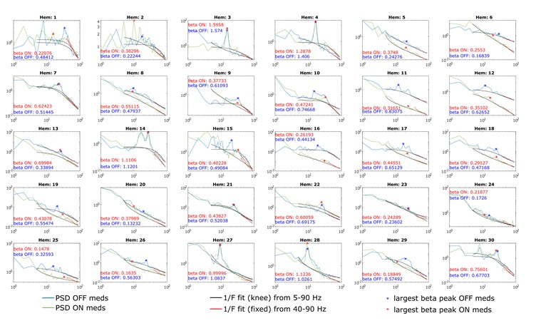
Figure R1. PSDs from all 30 hemispheres ON and OFF medication. Aperiodic fits are shown between 5-90 Hz (knee mode), which was used to calculate the power of beta peaks, and between 40-90 Hz (fixed mode), which was used to estimate the aperiodic exponent of the spectrum.
Another example is Fig. 1C, where the spectra for high and low STN spiking epochs are identical between 10 and 20 Hz, and the difference in higher frequency range could be well-explained by an overall increase of broadband gamma power (e.g. as observed in Manning et al., J Neurosci 2012, Ray & Maunsell PLoS Biol 2011). This increase of broadband gamma power is trivially expected, as broadband gamma power is tightly coupled with population spiking rate, which was used to define the two conditions.
We agree with the reviewer that in Figure 1C, high and low STN spiking states could well be separated by average gamma power (Figure 1E), too. However, the difference of aperiodic exponents is more prominent between both conditions (Figure 1D+E, based on p-values). What is more, in human LFP data recorded from clinical macroelectrodes, medication states can be reasonably well distinguished using the aperiodic exponent between 40-90 Hz (Figure 2C), but average gamma power does not separate both states (Figure S3A). This suggests that the aperiodic exponent reflects more than just power differences in the high gamma regions. In addition, power changes do not inevitably change the aperiodic exponent and vice versa as elaborated in (Donoghue et al., 2020).
Manning et al., 2009 show that the power spectrum is shifted to higher power values at all observed frequencies (2-150 Hz) as firing rates increase. As the reviewer points out, power spectra of our data are almost identical between 10-20 Hz (despite the marked spiking differences) and only drift apart from > 20 Hz (Figure 1C). This is a relevant difference between our study and Manning et al., 2009 and suggests that power differences in the gamma range are not solely explained by differences in spiking. This is confirmed when cortical activity at different spikes/sec is modelled (Miller et al., 2009). The entire spectrum is shifted to higher power values if spiking rates increase.
Ray & Maunsell, 2011 reported low (30-80 Hz) and high (> 80 Hz) gamma activity in the macaque visual cortex, with a positive correlation between spiking activity and high gamma activity. However, activities in the low gamma range (30-80 Hz), which largely overlaps with the frequency range in our study, does not necessarily correlate with firing rates.
In conclusion, the link between gamma power and spiking activity is not as strong as alluded. Even if the change in spiking activities can lead to changes of both gamma power and the aperiodic exponent, the aperiodic exponent would still constitute a measure to separate E/I levels and medication states.
The above consideration also speaks to a major weakness of the general approach of considering the 1/f spectrum a monolithic spectrum that can be captured by a single exponent. As the authors' Fig. 1C shows, there are distinct frequency regions within the 1/f spectrum that have different slopes. Indeed, this tripartite shape of the 1/f spectrum, including a "knee" feature around 40-70 Hz which is well visible here, was described in multiple previous papers (Miller et al., PLoS Comput Biol 2009; He et al., Neuron 2010), and have been successfully modeled with a neural network model using biologically plausible mechanisms (Chaudhuri et al., Cereb Cortex, 2017). The neglect of these fine-grained features confounds the authors' model fitting, because an overall increase in the broadband gamma power - which can be explained straightforwardly by the change in population firing rates - can result in the exponent, fit over a larger spectral frequency region, to decrease. However, this is not due to the exponent actually changing, but the overall increase of power in a specific sub-frequency-region of the broadband 1/f activity.
We have now used the knee mode for aperiodic fits between 5 and 90 Hz when periodic beta power is calculated. We agree that this broad frequency range is unlikely to have a single 1/f component.
We have also repeated the analysis of our animal data using the knee mode for aperiodic fits between 30 and 100 Hz (Figure S5). However, the goodness of fits had barely changed. In fact, the R2 and error become slightly worse. In addition, the knee parameter complicates interpretation of the aperiodic exponent and has to be considered along with the knee frequency. What is more, we do not see this bend around 40-70 Hz in all subjects. We show PSDs of representative LFP channels in Figure R2 and need to assert that the knee around 40-70 Hz is not a robust finding in our data set. Therefore, we chose the fixed mode for parameterisation within this frequency band.
Please see our answer to the previous comment regarding the link between broad gamma power and changes in population firing rates.
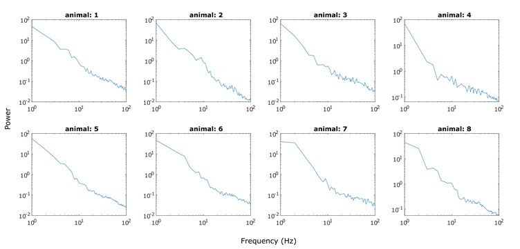
Figure R2. PSDs of representative PSD channels for each animal (data used in Figure 1C). The knee around 40-70 Hz is not a robust finding in all PSDs.
Author Response:
Reviewer #1:
The manuscript by Lalanne and Li aims to provide an intuitive and quantitative understanding of the expression of translation factors (TFs) from first principles. The authors first find that the steady-state solutions for translation sub-processes are largely independent at optimality. With a coarse-grained model, the authors derive the optimal expression of translation factors for all important sub-processes. The authors show that intuitive scaling factors can explain the differential expression of translation factors.
The results are impressive. However, as detailed in the major comments, the choice of some important parameters is not sufficiently justified in the current version. In particular, it is not clear to what extent parameter choice and rescaling was biased toward achieving a good agreement with the experimental data.
Major comments:
1) The work assumes that reaction times per TF are constant. That may be true at the highest growth rates, but it might not hold for conditions with lower growth rates. The data of Schmidt et al. (Nat. Biotechnol. 34, 104 (2016)) would allow to compare the predictions to proteome partitioning in E. coli across growth rates. It is ok to restrict the present work to maximal growth rates, but then this caveat should be made explicit. This last point also concerns ignoring the offset in the bacterial growth laws, which is only permissible at fast growth; that also should be stated more prominently in the manuscript; see also the legend of Fig. 1, "Our framework of flux optimization under proteome allocation constraint addresses what ribosome and translation factor abundances maximize growth rate".
We see two distinct but related points made by the reviewer, which we address in turn.
First, we thank the reviewer for highlighting the important and interesting point of the growth rate dependence of expression in components of the translational machinery, which encouraged us to investigate this aspect further. Leveraging other existing ribosome profiling datasets (which provide better quantitation than mass spectrometry data, see response to minor point #6 below) across multiple growth conditions and species, we compared the predicted optimal translation factor abundance in these conditions (using same formula for the optima). The new conditions and species now include E. coli at much slower growth rates, C. crescentus in two different media, and others. We found similar degrees of agreement between predicted and observed levels (shown in Figure 4-Figure supplement 1 ). One exception is aaRS in C. crescentus, and the discrepancy likely arises from a lack of quantification of tRNA abundance which is a parameter we use to predict the optimal aaRS levels.
These additional data also provided another way to examine the model predictions. Specifically, we assessed the predicted square-root scaling of translation factor abundance with growth rate. While the expression stoichiometry remains constant across growth rates (see response to minor point #6 below), the overall abundance decreases following our predicted scaling (Figure 4-Figure supplement 2B). We now describe these new analyses and results in the main text (p. 7, line 216):
"Analysis of tlF expression across slower growth conditions supports the derived square root dependence (Figure 4-Figure supplement 2)."
The second point made by the reviewer pertains to the “offset in bacterial growth law” that corresponds to inactive ribosomes, which make up a substantial fraction of ribosomes at very slow growth rates. We note that the derivation of the optimality condition, equation 5, does not rely on all ribosomes being active. What is necessary is that that there is a direct proteomic trade-off between ribosomes and translation factors (see response to minor point 1 below). To rigorously place our work in the context of previous literature, we have replaced mention of ribosome with “active ribosome” (as well as in equation 1 and Figure 1), which we define as those functionally engaged in the translation cycle. We also formally include the proteome fraction of inactive ribosome in equations 2 and 3 leading to the optimality condition.
2) The diffusion-limited regime considers only the free and idle reactants. For some translation factors, the free state only accounts for a small fraction of its total concentration. In this case, the diffusion-limited regime only explains a small fraction of the TFs. For example, most of EF-Ts may not be in its free state: in simulations with in vitro kinetics, free EF-Ts accounts for 6%-48% of its total concentration (Supplementary Data 3 in [21]). Can the authors use in vitro parameters (or other ways) to provide a rough estimate of the fraction of free TFs? Including this might allow to make quantitative statements about some of the deviations seen in Fig. 4, as most of the TFs are underestimated.
We thank the reviewer for the suggestion that deviations between the diffusion-limited prediction and the observed abundance might be quantitatively explained by the finite catalytic activity of the respective factors. However, to do so requires accurate values of kcat, which are often not available. In the Supplement of the initial submission, we provided an example of the in vitro kcat being not compatible with the protein synthesis rates in vivo, which we have now moved to the main text (reproduced below).
Another experimental approach that can feasibly be used to infer the bound fraction of translation factors in live cell is fluorescence microscopy of tagged proteins. Indeed, by quantifying the diffusive states of a tagged EF-Tu protein, Volkov et al (1) could estimate that <10% of EF-Tu was in its bound state, which is consistent with the agreement between our diffusion-limited prediction and observed abundance for that factor.
We now discuss these possibilities and the facts about EF-Ts in a paragraph in the Discussion (p. 13, line 471):
"Our optimization model can also be solved analytically in the non-diffusion-limited regime (Table 2), with the finite catalytic rate leading to an additional contribution of the form ∝ l 𝜆*/kcat. Recent detailed modeling of the EF-Ts cycle (Hu et al., 2020) estimated that a minor fraction (6 to 48%) of its abundance was in the free form in the cell, consistent with the large deviation we observe for this factor from our diffusion only prediction. However, the numerical values for these solutions are in general difficult to obtain because measurements of catalytic rates are sparse and often inconsistent with estimates of kinetics in live cells. As an example, the catalytic rates for aaRSs (Jeske et al., 2019) measured in vitro is ≈3 s-1 (median across different aaRSs), which is well below the minimal value of 15 s-1 required to sustain translation flux at the measured translation elongation rate (Appendix 5), suggesting substantial deviation between in vitro and in vivo kinetics. Although technically demanding, the fraction of free vs. bound factors can in principle be determined through live cell microscopy of tagged factors based on the partitioning the diffusive states of enzymes. Using that approach, (Volkov et al., 2018) estimated that EF-Tu was in its bound state <10% of the time (consistent with the agreement between our diffusion-limited prediction and the observed value for this factor)."
3) "A factor-independent time τ_ind (e.g., peptidyl transfer), which does not come into play in our optimization framework, was added to account for additional steps making up the full elongation cycle." - what happened to this time? I couldn't find it anywhere else in the paper. What value was chosen, and by what rationale?
We thank the reviewer for pointing out a lack of clarity in our presentation. The factor-independent time τind in fact did not appear in our optimization procedure at all (by virtue of obeying dτind/d𝜙TFi = 0 by definition), and was only included for generality to account for steps such as peptidyl transferase (extremely fast (2)). In line with the parsimony of our model, and to avoid any confusion, we have now removed this factor from our model and description altogether.
4) Fig. 4: The agreement is very impressive, especially given the simplifying assumptions. However, there are some questions relating the choice of parameters.
a) Were any parameters fitted? Which, how? What about τ_ind, for example (see above)?
Our approach does not include any fitted parameter. We instead rely on biophysically measured quantities such as diffusion constants, protein sizes, tRNA abundances, cell doubling times (growth rates), and in vivo kinetic estimates. (In the line of Major Comment #3 above, we have removed τind for clarity.) We now include all quantities needed to predict the optimal translation factor abundances (using the formula listed in section “Summary of optimal solutions”, Table 2) in Appendix 5-Tables 1-3, including new Appendix 5-Tables 2-3, reproduced below.
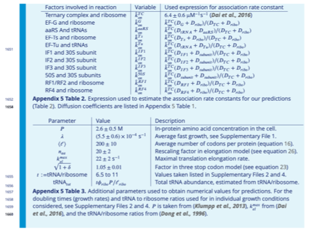
b) The "predicted" value for ribosomes is calculated from observed data (in a way described on p. S34 that I found incomprehensible, and would likely look very similar regardless of the predicted values for the TFs). According to the section "Equipartition between TF and corresponding ribosomes", the corresponding ribosomes can be quantified in the authors' scheme, too, by the method used for deriving optimal TF concentrations in equation 5. Why didn't the authors directly use the sum of these estimations as the optimal ribosome concentration in Fig. 4? In the current state, it does not seem fair to include the ribosome with the other predictions.
We agree that the nature of the prediction for ribosomes was different than for other translation factors in our original manuscript in a way that might have lacked clarity. We now exclude ribosomes from Fig. 4 to avoid any possible confusion.
It is interesting to directly estimate ribosome abundance using the equipartition principle. This estimation is however limited by the fact that the equipartition principle only accounts for ribosomes that are waiting for factor- dependent binding steps. Substantial fractions of ribosomes may be engaged at factor-free steps (e.g., peptidyl transfer catalyzed by ribosome itself) and factor-dependent catalytic steps after binding. Although the latter could be estimated using the observed tlF concentrations (by considering that the tlF in excess to the binding-limited predictions is sequestered in catalytic steps), the former is not estimated in our model. Furthermore, some other ribosomes may not be fully assembled yet or are inactive (3). Indeed, the predicted factor-dependent ribosome abundance using the equipartition principle with observed tlF abundances constitute a fraction (40%) of the measured total ribosome abundance.
c) Predictions are for a specific growth rate (doubling time 21min). Was this growth rate also averaged over the three organisms? What were the individual values? These points would need to be discussed in the main text.
The reviewer is correct. In the initial submission, we used the average growth rate of E. coli (doubling time 21.5±0.4 min), B. subtilis (doubling time 21±1 min), and V. natriegens (doubling time 19±1 min). A note has been added in the main text (p. 11, line 448):
"We take the growth rate 𝜆* to be the average of the fast-growing species considered, corresponding to a doubling time of 21±1 min (E. coli: 21.5±1 min, B. subtilis: 21±1 min, V. natriegens: 19±1 min)."
In addition, we now include predictions for different growth rates and compared them with several bacterial species grown in a wide range of conditions (Figure 4-Figure supplement 1) (see response to Major Comment #1 and to reviewer 2’s third request). These predictions and data are now included in Supplementary Files 1-4.
5) In the same vein, in a footnote (!) to Table S4: "#For the ternary complex, the total mass of tRNA+EF-Tu was converted to an equivalent amino acid length." - I can see that this is important to get reasonable results, but it constitutes a major deviation from the strategy proclaimed throughout the main text: that the predicted effects result from a competition for fractions of the limited proteome. That rationale has to be changed (and explained in the main text), or the predictions in Fig. 4 should be based on calculations using only the protein part of TCs (i.e., EF-Tu).
We are sorry for the confusion. The procedure of converting tRNA size to protein size was only used to estimate diffusion coefficients for the ternary complex (described in Appendix 5 Table 2), and not for the competition within the proteome. For factors for which no direct experimental estimates exist for in vivo diffusion coefficient, we used the relationship DA = (lTC/lA)1/3 DTC. The resulting estimated diffusion coefficients were then used to rescale the association rate inferred from in vivo measurements for the ternary complex (see response to point 6 below as well) to obtain association rates for other factors.
6) S9: "we anchored our association rates to the estimated in vivo association rate for the ternary complex, 𝑘^𝑇𝐶 = 6.4 μM−1s−1 [13], and rescale the association rate by diffusion of related components" - in comparison, the diffusion limited k^TC is >100. If I understand this correctly, you simply rescale ALL on-rates by 100/6.4 = 15.6. If that is (qualitatively) correct, you would need to discuss this point (and the derivation of the scaling factor) explicitly in the main text.
The reviewer is correct in his interpretation of our approach, and we are grateful for his remark as this led us to spot a mistake in our choice of parameter (capture radius R). Indeed, while the ternary complex as a largest physical dimension of about 10 nm (from structural data (4)), the appropriate capture radius is closer to 2 nm (size of the portion binding to the ribosome) (5). Correcting for the appropriate capture radius alone brings the estimate to 45 μM-1s-1 , which is however still several-fold higher than the measured value of 6.4 μM-1s-1. Whereas a part of this could be due to systematic overestimation of the diffusion coefficient, a large portion of the discrepancy is assuredly due to the many simplifying assumptions underlying the Smoluchowski estimate which serve to place an absolute upper bound on the reaction rate (perfectly/instantaneously absorbing spheres, and hence no notion of specific reaction position or molecular orientation).
The estimate for capture radius R has been corrected (p. 47, line 1605) and a new sentence has now been included in the main text (p. 11, line 441):
"Importantly, the absolute values of the optimal concentrations can be anchored by the association rate constant between TC and the ribosome obtained from translation elongation kinetic measurements in vivo (Dai et al., 2016). The latter was found to be several-fold smaller than the simplest and absolute upper bound of a Smoluchowski estimate of perfectly absorbing spheres (section Estimation of optimal abundances), and we assume that the rescaling factor is the same for all reactions."
Author Response
Reviewer #1 (Public Review):
Iyer et al. address the problem of how cells exposed to a graded but noisy morphogen concentration are able to infer their position reliably, in other words how the positional information of a realistic morphogen gradient is decoded through cell-autonomous ligand processing. The authors introduce a model of a ligand processing network involving multiple ”branches” (receptor types) and ”tiers” (compartments where ligand-bound receptors can be located). Receptor levels are allowed to vary with distance from the source independently of the morphogen concentration. All rates, except for the ligand binding and unbinding rates, are potentially under feedback control. The authors assume that the cells can infer their position from the output of the signalling network in an optimal way. The resulting parameter space is then explored to identify optimal ”network architectures” and parameters, i.e. those that maximise the fidelity of the positional inference. The analysis shows how the presence of both specific and non-specific receptors, graded receptor expression and feedback loops can contribute to improving positional inference. These results are compared with known features of the Wnt signalling system in Drosophila wing imaginal disc.
The authors are doing an interesting study of how feedback control of the signalling network reading a morphogen gradient can influence the precision of the read-out. The main strength of this work is the attention to the development of the mathematical framework. While the family of network architectures introduced here is not completely generic, there is enough flexibility to explore various features of realistic signalling systems. It is exciting to find that some network topologies are particularly efficient at reducing the noise in the morphogen gradient. The comparison with the Wnt system in Drosophila is also promising.
Major comments:
1) The authors assume that the cell estimates its position through the maximum a posteriori estimate, Eq.(5), which is a well-defined mathematical object; it seems to us however that whether the cell is actually capable of performing this measurement is uncertain (it is an optimal measurement in some sense, but there is no guarantee that the cell is optimal in that respect). Notably, this entails evaluating p(theta), which is a probability distribution over the entire tissue, so this estimate can not be done with purely local measurements. Can the authors comment on this and how the conclusions would change if a different position measurement was performed?
This is indeed an important question. Our viewpoint is that if the cells were to use a maximum a posteriori (MAP) estimate (Eq. 5) to decode their positions, then what features of the channel architecture would lead to small errors in positional inference. Whether the maximum a posteriori estimate is employed by the cell, or some other estimate, is an important but difficult question to address. Our choice has been motivated by how this estimate has allowed the precise determination of developmental fates in the context of gap gene expression in Drosophila embryo [1, 2, 3]. We had earlier computed the inference error with a different estimate i.e.
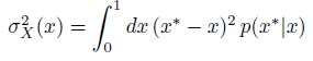
which computes the mean squared deviations of the inferred positions from the true position for each x, taking into account the entire distribution p(x∗|x). While the qualitative results are the same, the inference errors showed spurious jitters from outliers in sampling the noisy morphogen input distribution. This consistency might suggest that our qualitative results are insensitive to the choice of the estimate.
Further, when evaluating the MAP estimate, the term p(θ) in the denominator serves as a normalisation factor to ensure p(x|θ) is a probability density. This is not strictly necessary for MAP estimation. Since p(θ) does not depend on x, the MAP estimate can be written as follows
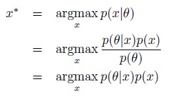
without the need for evaluating p(θ). In the case of a uniform prior, it would be equivalent to maximum likelihood estimate (MLE) i.e.
2) One of the features of the signalling networks studied in the manuscript is the ability of the system to form a complex (termed a conjugated state, Q) made of two ligands L, one receptor and one nonsignalling receptor. While there are clear examples of a single ligand binding to two signalling receptors (e.g. Bmps), are there also known situations where such a complex with two ligands, one receptor, and one non-signalling receptor can form? In the Wnt example (Fig. 10a), it is not clear what this complex would be? In general, it would be great to have a more extended discussion of how the model hypothesis for the signalling networks could relate to real systems.
This is a good suggestion. We have now added a discussion on the various possible realisations of the “conjugate state” Q in Section 3.6. We have also explored the various states in the context of different signalling contexts such as Dpp, Hh, Fgf in the Discussion section.
The conjugated state ‘Q’ represents a combination of the readings from the two branches i.e. receptor types. This could be realised through processes like ligand exchange or complex formation, both in a shared spatial location such as a compartment. As discussed in the original manuscript (Section 3.6 of the revised manuscript), the ligand Wg in the Wg signalling pathway is internalised through two separate endocytic pathways associated with the receptor types - signalling receptor Frizzled (via Clathrin-mediated endocytosis (CME)) and non-signalling receptor HSPGs (via the CLIC/GEEC pathway (CLIC - (clathrin-independent carriers, GEEC - GPI-anchored protein-enriched early endosomal compartments)). Both pathways meet in a common early endosomal compartment where the ligands may be exchanged between the two receptors [4]. In a previous work by Hemalatha et al [4], we had shown that there are more Wg-DFz2 interactions in the endosomal compartment (measured through FRET) than on the cell surface. Therefore, the non-signalling receptors directing Wg through the CLIC/GEEC pathway titrate the amount of Wg interaction with the signalling receptor, DFz2.
As mentioned in the original manuscript (Section 3.3 and subsection 4.2 of the Discussion in the revised manuscript), apart from Wg signalling, non-signalling receptors such as the HSPGs have also been proposed to act as co-receptors for Dpp, Hh, FGF (reviewed in [5, 6]). Although some ligands bind to the core protein of HSPG, the majority of the ligands bind to the negatively charged HS chains [7, 8]. Here, the coreceptors HSPGs aid in capturing diffusible ligands and presenting the same to signalling receptors (either on the cell surface or within endosomes).
3) The authors consider feedback on reaction rates - it would seem natural to also consider feedback on the total number of receptors; notably, since there are known examples of receptors transcriptionally down-regulated by their ligands (e.g. Dpp/Tkv)? Also it is not clear in insets such as in Fig. 7b, if the concentration plotted corresponds to the concentration of receptors bound to ligands?
As mentioned in the original manuscript (Section 2.2 of the revised manuscript), we have indeed considered control on reaction rates and receptors, although the control on the latter is done with the constraint of receptor profiles being monotonic. Further, while the control on reaction rates is considered via feedbacks explicitly, the control on receptors is done via an approach akin to the openloop control used in control theory. In reality, cellular control on receptors will involve transcriptional up- or down-regulation of receptor and thus warrant a feedback control approach – however, the timescales involved in such a control are different from the binding-unbinding and signalling timescales.
Therefore, in the current work, we take the morphogen profile to be given i.e. independent of receptor concentrations, and we ask for the receptor concentrations that would help reduce the inference errors.
Our predictions of increasing signalling receptor and decreasing non-signalling receptors in a twobranch channel architecture are consistent with the known transcriptional up-regulation of Dally/Dlp and down-regulation of Fz by Wg signalling [9].
In a future work, we will extend the control on receptors to include feedbacks explicitly. Furthermore, the explicit feedback control on receptors may need to be considered concomitantly with the effect of receptors on morphogen dynamics (i.e. morphogen sculpting by receptors) along with the possibility of spatial correlations in receptor concentrations through neighbouring cell-cell interactions.
As mentioned in the original manuscript (Section 2.2 of the revised manuscript), the variables ψ and φ stand for the total (bound + unbound) surface receptor concentrations of the signalling and the non-signalling receptors respectively. Therefore, the insets showing receptor profiles such as in Fig. 6b, 7b, and Appendix H Fig.8b,e correspond to the total surface receptor concentrations.
4) The authors are clear about the fact that they consider the morphogen gradient to be fixed independently of the reaction network; however, that seems like a very strong assumption; in the Dpp morphogen gradient for instance over expression of the Tkv receptor leads to gradient shortening. Can the authors comment on this?
This point is related to the earlier question 4. As discussed in the Discussion of the original manuscript (subsection 4.3 of the revised manuscript), we focus on finding the optimal receptor concentration profiles and reaction networks that enable precision and robustness in positional information from a given noisy morphogen profile. The framework and the optimisation scheme within it will prescribe different receptor profiles and reaction networks for different monotonically behaving, noisy morphogen profiles. It is possible that cells may achieve the optimal receptor concentrations via feedback control on production of the receptors.
Broadly, morphogen dynamics depends on cell surface receptors, which could participate in both the inference and the sculpting of the morphogen profile, and factors independent of them such as extracellular degradation, transport and production, etc. In our present work, we have taken the receptors involved in sculpting and inference as being independent.
In a more general case, feedback control on receptors will change the receptor concentrations as well as the morphogen profile. We are currently working on realising such a feedback control on receptors within the same broader information theoretic framework proposed in the current work.
5) Fig. 10f is showing an exciting result on the change in endocytic gradient CV in the WT and in DN mutant of Garz. Can the authors check that the Wg morphogen gradient is not changing in these two conditions? And can they also show the original gradient, and not only its CV?
The reviewer raises a legitimate concern – could the observed changes in CV upon perturbation of endocytic machinery be attributed to a systematic change in the mean levels of the endocytosed Wg alone? In the original manuscript (Appendix O Fig.17b,c of the revised manuscript), we show the normalised profiles of endocytic Wg in control and myr-Garz-DN cases. Here, in Fig.1 below, we show a comparison between the mean Wg concentrations (measured as fluorescence intensity) in control wing discs and discs wherein CLIC/GEEC endocytic pathway is removed using UAS-myr-Garz-DN. For clarity, we show the discs with largest and smallest fluorescence intensities from the control and myr-Garz-DN discs. It is hard to conclude that the mean concentrations are significantly different in the two cases.
Reviewer #2 (Public Review):
The work of Iyer et al. uses a computational approach to investigate how cells using multiple tiers of processing and multiple parallel receptor types allow more accurate reading of position from a noisy signal. Authors find that combining signaling and non-signaling types of receptors together with additional feedback increases the accuracy of positional readout against extrinsic noise that is conveyed in the morphogen signal. Further, extending the number of layers of signal processing counteracts the intrinsic stochasticity of the signal reading and processing steps. The mathematical formulation of the model is general but comprehensive in the way it handles the difference between branches and tiers for the processing of channels with feedbacks. The results of the model are presented from simple one-branch and one-tier architecture to two-branch and two-tier architecture with feedbacks. Interestingly authors find that adding more tiers results in only very small improvements in the accuracy of positional readout. The model is tested against a perturbation experiment that impairs one of the signaling branches in the Drosophila wing disc, but the comparison is only qualitative as further experiment-oriented work is planned in a separate paper.
Strengths
There is a clear statement of objectives, model, and how the model is evaluated. In particular, the objective is to find what number of receptor types and their concentrations for a given number of tiers and feedback types is resulting in the most accurate positional readout. The employed optimization procedure is capable to find signalling architectures that result in one cell diameter positional precision for most of the tissue with 3-4 cells at the tissue end that is most distant to the morphogen source. This demonstrates that employing additional complexity in signal processing results in a very accurate positional readout, which is comparable with estimates of positional precision obtained in other developmental systems (Petkova et al., Cell 2019, Zagorski et al., Science 2017).
The optimal signalling architectures indicate that both signalling (specific) and non-signalling (nonspecific) receptors affect the precision of positional readout, but the contributions of each type of these receptors are qualitatively different. Even slight perturbation of signalling receptors drives the system out of optimum, resulting in a decrease in positional precision. In contrast, the non-signalling receptors could accommodate much larger perturbations. This observation could provide a biophysical explanation for how cross-talk between different morphogen species could be realized in a way that positional precision is kept at the optimum when morphogen signaling undergoes extrinsic and intrinsic perturbations.
Last, the model formulation allows to specifically address perturbations of signalling and feedbacks, that could be explored to validate model predictions experimentally in Drosophila wing disc, but also in other developmental tissues. The authors present a proof-of-concept by obtaining consistent results of variation of output profiles in two-tier two-branch architectures with non-signaling branch removed and intensity profiles of Wg in wing disc where the CLIC/GEEC endocytic pathway was perturbed.
Weaknesses
The list of model parameters is long including more than 20 entries for two-tier two-branch architectures. This is expected, as the aim of the model is to describe the sophisticated signalling architecture mimicking the biological system. However, this also makes it very challenging or impossible to provide guiding principles or understanding of the system behaviour for the complete space of signalling architectures that optimize positional readout. Although, the employed optimization procedure finds solutions that exhibit very high positional accuracy, there is only very limited notion how these solutions depend on variation of different parameters. The authors do not address the following question, whether these solutions correspond to broad global optima in the space of all solutions, or were rather fine-tuned by the optimization procedure and are quite rare.
It is unclear how contributions from the intrinsic noise affect the system behaviour compared to contributions from extrinsic noise. In principle, the two-branch one-tier architecture results in an already very accurate positional readout across the tissue. The adding of another tier seems to provide only a very weak improvement over a one-tier solution. It is possible that contributions from intrinsic noise for the investigated signalling architectures are only mildly affecting the system compared with contributions from extrinsic noise. Hence, it is difficult to assess whether the claim of reducing intrinsic noise by adding another tier is supported by the presented data, as the contributions from intrinsic noise could overall very weakly affect the positional readout.
The optimal response of the channel to extrinsic and intrinsic noises is very distinct. As noted correctly by the reviewer, an additional tier provides only a marginal improvement in inference error due extrinsic noise (compare Fig.7 and Fig.8 in the revised manuscript). However, as shown in Fig.9c of the revised manuscript (same as in the original manuscript), adding an extra tier provides a substantial improvement in inference errors due to intrinsic noise.
References
[1] Gasper Tkacik, Julien O Dubuis, Mariela D Petkova, and Thomas Gregor. Positional information, positional error, and readout precision in morphogenesis: a mathematical framework. Genetics, 199:39– 59, 2015.
[2] Mariela D Petkova, Gasper Tkacik, William Bialek, Eric F Wieschaus, and Thomas Gregor. Optimal decoding of cellular identities in a genetic network. Cell, 176:844–855, 2019.
[3] Julien O Dubuis, Gaˇsper Tkaˇcik, Eric F Wieschaus, Thomas Gregor, and William Bialek. Positional information, in bits. Proceedings of the National Academy of Sciences, 110:16301–16308, 2013.
[4] Anupama Hemalatha, Chaitra Prabhakara, and Satyajit Mayor. Endocytosis of wingless via a dynaminindependent pathway is necessary for signaling in drosophila wing discs. Proceedings of the National Academy of Sciences, 113:E6993–E7002, 2016.
[5] Xinhua Lin. Functions of heparan sulfate proteoglycans in cell signaling during development. Development, 131:6009–6021, 2004.
[6] Stephane Sarrazin, William C Lamanna, and Jeffrey D Esko. Heparan sulfate proteoglycans. Cold Spring Harbor perspectives in biology, 3(7):a004952, 2011.
[7] Catherine A Kirkpatrick, Sarah M Knox, William D Staatz, Bethany Fox, Daniel M Lercher, and Scott B Selleck. The function of a drosophila glypican does not depend entirely on heparan sulfate modification. Developmental biology, 300(2):570–582, 2006.
[8] Mariana I Capurro, Ping Xu, Wen Shi, Fuchuan Li, Angela Jia, and Jorge Filmus. Glypican-3 inhibits hedgehog signaling during development by competing with patched for hedgehog binding. Developmental cell, 14(5):700–711, 2008.
[9] Kenneth M Cadigan, Matthew P Fish, Eric J Rulifson, and Roel Nusse. Wingless repression of drosophila frizzled 2 expression shapes the wingless morphogen gradient in the wing. Cell, 93(5):767–777, 1998.
Author Response
Reviewer #1 (Public Review):
Strength: The study is summarizing a large cohort of human samples of blood, nasal swabs and nasopharyngeal aspirates. This is very uncommon as most of the time studies focus on the blood and serum of patients. Within the study, 3 monocyte and 3 DC subsets have been followed in healthy and Influenza A virus-infected persons. The study also includes functional data on the responsiveness of Influenza A virus-infected DC and monocyte populations. The authors achieved their aims in that they were able to show that the tissue microenvironment is important to understand subset specific migration and activation behavior in Influenza A virus infection and in addition that it matters with which kind of agent a person is infected. Thus, this study also impacts a better understanding of vaccine design for respiratory viruses.
We thank Reviewer 1 for highlighting what we believe to be the greatest strengths of our study. The key feature of this study was to generate a comprehensive description of monocytes and dendritic cells (DC) in the human nasopharynx during influenza A virus infection, and to provide a comparison with healthy and convalescent individuals. Further, we wished to emphasize the value of studying the nasopharynx during respiratory viral infections, particularly in light of the ongoing COVID-19 pandemic. We describe a non-invasive method to (longitudinally) sample this anatomical compartment that allows retrieval of intact immune cells as well as mucosal fluid for soluble marker analysis. We also believe that the addition of proteomic profiles in the different compartments (new Figure 7) further highlights the importance of the tissue microenvironment.
Weakness: In the described study, the authors used a different nomenclature to introduce the DC subsets. This is confusing and the authors should stick to the nomenclature introduced by Guilliams et al., 2014 (doi.org/10.1038/nri3712) and commented in Ginhoux et al., 2022 (DOI: 10.1038/s41577-022-00675-7 ) or at least should introduce the alternative names (cDC1, cDC2, expression markers XCR1, CD172a/Sirpa). Further, Segura et al., 2013 (doi: 10.1084/jem.20121103) showed that all three DC subpopulations were able to perform cross-presentation when directly isolated. Overall, a more up-to-date introduction would be useful.
Reviewer 1 commented on the DC nomenclature used in the manuscript. We agree that our manuscript would benefit from appropriately updating the DC nomenclature. We therefore revised the text, and now we refer to the subsets previously described as CD1c+ and CD141+ myeloid DCs (MDC) as cDC2 and CDC1 subsets, respectively. We have also modified the text in the Introduction of the revised manuscript to reflect the same and give a more up-to-date introduction of DC subsets (marked-up version lines 75-81).
As the data of this was already obtained in 2016-2018 it is clear that the FACS panel was not developed to study DC3. If possible, the authors might be able to speculate about the role of this subset in their data set. Moreover, there were other studies on SARS-CoV-2 infection and DC subset analyses in blood (line 87, and line 489) e.g. Winheim et al., (DOI: 10.1371/journal.ppat.1009742 ), which the authors should introduce and discuss in regard to their own data.
As reviewer 1 accurately pointed out, the flow cytometry panel used in this study was indeed not developed to study the DC3 subset. The data was obtained in 2016-2018, and lack the typical markers used to identify the DC3 subset, such as CD163, BTLA and CD5 (Cytlak et al, https://doi.org/10.1016/j.immuni.2020.07.003, Villani et al, https://doi.org/10.1126/science.aah4573). Due to the constraints of the panel, we would not be able to accurately identify DC3s. However, in an attempt to dig deeper into the data that is available, we re-analyzed the data to identify CD14+CD1c+ cells among the lineage–HLADR+CD16–CD14+ cells, here collectively called “mo-DC”. This population is likely a combination of monocytes upregulating CD1c and bona fide DC3 expressing CD14. Accordingly, the gating strategy was updated in Supplementary figure 1 (marked-up version lines 192-194), and new data plot in Figure 2H (marked-up version lines 208-220) summarizes the changes observed in mo-DC numbers in IAV patients between blood and the nasopharynx. Parallel to the pattern seen in other DC subsets, mo-DC frequencies are reduced in blood and we observed an increase (not significant) in the nasopharynx.
As CD88 was not included in the original panel, it was not possible to discriminate between bona fide monocytes and DC3s. We performed a staining of PBMCs (buffy coat) with CD88 (FITC) added to the original flow panel used in the study, to assess if CD88 can be helpful for future studies (Reviewer figure 1). The staining showed that some cells in the mo-DC population are CD88 positive, indicating a bona fide monocyte origin, whereas some are negative, indicating that they are bona fide DC3 expressing CD14. (Bourdely et al, https://doi.org/10.1016/j.immuni.2020.06.002).
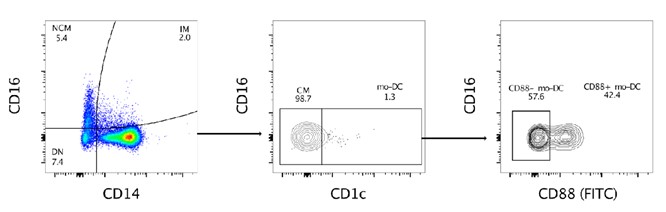
Reviewer figure 1. Expression of CD88 in the “mo-DC” population. Cells from a buffy coat were stained with the flow cytometry panel used in the manuscript, with the addition of CD88 (FITC). Within the CD14+CD1c+ population, the “mo-DC” population, we identified both CD88+ and CD88- cells.
Reviewer 1 also suggested citing Winheim et al (https://doi.org/10.1371/journal.ppat.1009742), and we thank them for their suggestion. We have now cited Winheim et al, and two additional reports (Kvedaraite et al, https://doi.org/10.1073/pnas.2018587118 and Affandi et al, https://doi.org/10.3389/fimmu.2021.697840) describing a depletion of DC3s (and other DC subsets) from circulation, and functional impairment of DCs following SARS-CoV-2 infection. Further, Winheim et al observed an increased frequency of a CD163+CD14+ subpopulation within the DC3s, which correlated with systemic inflammatory responses in SARS-CoV-2 infection. We speculate that perhaps in IAV infection too, DC3s may follow the trend of other DC subsets and be found in increased numbers in the nasopharynx (marked-up version lines 75-81 and 543-552).
Taken together, although the data are very important and very interesting, my overall impression of the manuscript is that in the era of RNA seq and scRNA seq analyses the study lacks a bit of comprehensiveness.
The final comment from reviewer 1 is well taken, in that our study does not include RNA-seq analyses. Again, we ask Reviewer 1 to take into consideration the challenging material we worked with in our study in combination with the COVID-19 pandemic that subsequently has excluded recruitment of new influenza patients to the study. The cell numbers and viability in the nasopharyngeal aspirates limit what experimental approaches can be done simultaneously, and flow cytometry seemed to be the best approach for the study. However, we agree that in future studies, both our own and those of others in the field, will greatly benefit from single cell analysis of nasopharyngeal immune cells, and from generating transcriptomic or epigenetic profiles of these cells. Unfortunately, it is a limitation that we are currently unable to overcome within the scope of this revision. Despite this weakness, we agree with Reviewer 1 that the methods we developed and the data we generated are important and interesting.
Moreover, we have added additional proteomics data from both NPA and plasma from influenza and COVID-19 patients, using the SomaScan platform (new Figure 7) (marked-up version lines 472-511, 738-755 and 768-792). We also included a supplementary table listing enriched pathway data from gProfiler. Briefly, our data showed sizeable changes within the blood and nasopharyngeal proteome during respiratory virus infection (IAV or SARS-CoV-2), as compared to healthy controls. Importantly, we found several differentially expressed proteins unique to the nasopharynx that were not seen in blood, and pathway analysis highlighted “host immune responses” and “innate immunity” pathways, containing TNF, IL-6, ISG15, IL-18R, CCL7, CXCL10 (IP-10), CXCL11, GZMB, SEMA4A, S100A8, S100A9. These findings are in line with our flow cytometry data, and support our hypothesis that the immunological response to viral infection in the upper airways differ from that in matching plasma samples. One of the main messages in this manuscript is the importance of looking at the site of infection, and not only at systemic immune responses to better understand respiratory viral infections in humans. We believe that the addition of the proteomics data serves to further highlight this point.
Reviewer #2 (Public Review):
This study aims to describe the distribution and functional status of monocytes and dendritic cells in the blood and nasopharyngeal aspirate (NPA) after respiratory viral infection in more than 50 patients affected by influenza A, B, RSV and SARS-CoV2. The authors use flow cytometry to define HLA-DR+ lineage negative cells, and within this gate, classical, intermediate and non-classical monocytes and CD1c+, CD141+, and CD123+ dendritic cells (DC). They show a large increase in classical monocytes in NPA and an increase in intermediate monocytes in blood and NPA, with more subtle changes in non-classical monocytes. Changes in intermediate monocytes were age-dependent and resolution was seen with convalescence. While blood monocytes tended to increase in blood and NPA, DC frequency was reduced in blood but also increased in NPA. There were signs of maturation in monocytes and DC in NPA compared with blood as judged by expression of HLA-DR and CD86. Cytokine levels in NPA were increased in infection in association with enrichment of cytokine-producing cells. Various patterns were observed in different viral infections suggesting some specificity of pathogen response. The work did not fully document the diversity of human myeloid cells that have arisen from single-cell transcriptomics over the last 5 years, notably the classification of monocytes which shows only two distinct subsets (intermediate cannot be distinguished from classical), distinct populations of DC1, DC2 and DC3 (DC2 and 3 both having CD1c, but different levels of monocyte antigens), and the lack of distinction provided by CD123 which also includes a precursor population of AXL+SIGLEC6+ myeloid cells in addition to plasmacytoid DC. Furthermore, some greater precision of the gating could have been achieved for the subsets presented. Specifically, CD34+ cells were not excluded from the HLA-DR+ lineage- gate, and the threshold of CD11c may have excluded some DC1 owing to the low expression of this antigen. Overall, the work shows that interesting results can be obtained by comparing myeloid populations of blood and NPA during viral infection and that lineage, viral and age-specific patterns are observed. However, the mechanistic insights for host defense provided by these observations remain relatively modest.
We thank Reviewer 2 for their assessment of our manuscript and summarizing our key findings in their public review. As reviewer 2 noted, our study describes changes in frequencies of monocytes and DCs during acute IAV infection, in blood and in the nasopharynx. Additionally, we also demonstrate pathogen-specific changes in both compartments. Reviewer 2 also highlighted a drawback of our study- that the approach did not fully capture the breadth of monocyte and DC diversity as it currently stands. Despite this, the findings we presented here laid the groundwork for continued research and led to significant progress, including mechanistic insights (Falck-Jones et al, https://doi.org/10.1172/JCI144734 and Cagigi et al, https://doi.org/10.1172/jci.insight.151463, Havervall et al. https://doi.org/10.1056/nejmc2209651 and Marking et al. Lancet Infectious Diseases in press), in understanding the role of myeloid cells in the human airways during viral infections.
Author Response
Reviewer #1 (Public Review):
In the article "Whole transcriptome-sequencing and network analysis of CD1c+ human dendritic cells identifies cytokine-secreting subsets linked to type I IFN-negative autoimmunity to the eye," Hiddingh, Pandit, Verhagen, et al., analyze peripheral antigen presenting cells from patients with active uveitis and control patients, and find several differentially expressed transcription factors and surface markers. In addition, they find a subset of antigen presenting cells that is decreased in frequency in patients with uveitis that in previous publications was shown to be increased in the eye of patients with active uveitis. The greatest strength of this paper is the ability to obtain such a large number of samples from active uveitis patients that are not currently on systemic therapy. While the validation experiments have methodologic flaws that decrease their usefulness, this study will still serve as a valuable resource in generating hypotheses about the pathogenesis of uveitis that can be tested in future projects.
We thank the reviewer for the constructive comments and effort to review our work in detail.
Since all CD36+CX3CR1+ cells are CD14+ (Figure 4D), how CX3CR1 ended up being differentially regulated in a similar way despite this population was excluded from 2nd bulk RNAseq data set should be commented on by the authors.
We agree with reviewer that the CD14 surface expression in relation to the black-gene module and CD36+CX3CR1+ DC3s requires more detailed analysis. As described in the results section, genes in this module are linked to both CD1c+ DCs and inflammatory CD14+ monocytes, which we cannot distinguish by bulk RNA seq analysis. Therefore, we aimed to use an approach to demonstrate that the black module is a bona fide CD1c+ DC gene signature not dependent on CD14 surface expression: We showed that there was not difference in CD14+ cell fractions in the samples for RNA-seq between patient and control samples (see Fig. 1F). We now further investigated this by additional data and experiments. We now show in Figure 2 Supplement 2A that CD14 – as expected - does not correlate with the black module. To confirm this experimentally, we purified CD14+CD1c+ and CD14- CD1c+ DCs from 6 donors and subjected these to qPCR analysis to evaluate the expression of key genes from the black module (see revised Figure 2A). As illustrated in revised Figure 2 panel B, we show that the expression levels of genes, including CD36 and CX3CR1, are not significantly altered between CD14+/- CD1c+ DCs which supports that the identified gene module is also not dependent on CD14 surface expression by CD1c+ DCs. To assess if the expression of the black module was also independent of CD14 in inflammatory disease, we used RNA-seq data from FACS-sorted CD14+CD1c+ DCs and CD14-CD1c+ DCS from patients with SLE and Scleroderma (GSE13731) and confirm that the expression of the black module genes is independent from CD14 surface expression (see revised Figure 2 panel C). Finally, we removed CD14+ cells from the analysis in the 2nd bulk RNA-seq experiment to proof that indeed the black module could be perceived as being associated with uveitis independent of CD14+ expression which allowed attributing the black module to CD1c+ DCs by bulk RNA-seq analyses. Also, more detailed analysis by flow cytometry (Revised Figure 4) and scRNA-seq (Figure 6) confirm these findings. For example, we show that the CD36+ CX3CR1+ DC3s are in fact a subset of CD14+ CD1c+ DCs (Figure 2 – Supplement 2) and we show that eye-infiltrating CD1c+ DCs that harbor the black module gene signature show increased CD36 and CX3CR1, but not CD14 (Figure 6C). We have addressed all these experiments and data in the result section on page 12-13, 16,17, and in the discussion section on page 19. We hope the reviewer agrees that this has now been sufficiently addressed.
Line 153: "...substantiates this gene set as a core transcriptional feature of human autoimmune uveitis." It would be difficult to argue that when only 137 of the 1236 DEGs from the first module are repeated in a validation data set that this is the core transcriptions set that defines the population in any uveitis. Further concerns include that the validation data set is not the same population, but rather a subset not containing CD14.
We agree with the reviewer and have changed this in the result section to “substantiates this gene set as a robust and bona fide transcriptional feature of CD1c+ DCs in human non-infectious uveitis” at page 13. We agree that - as expected - the removal of CD14+ cells impacted the sensitivity of our analysis, but that this strategy was required to attribute the black module to CD1c+ DCs. Our data supports that the black module gene signature is not restricted to CD14+ CD1c+ DCs by demonstrating that its dysregulation in non-infectious uveitis can even be perceived in CD14- CD1c+ DCs. We show now that the replication of a fraction of genes of the black module is a consequence of sensitivity to detect differentially expressed genes (Figure 2 – Supplement 1C). – most likely due to lower cell number after sorting out CD14+ cells. We have outlined this in greater detail in the result section on page 13. We hope the reviewer agrees this has now been adequately described.
Line 220: Notch-dll experiments: with the experiments presented it is not possible to say that the changes are due to maintenance of CD1c+ DCs without further experiments outlining what NOTCH2 signaling changes throughout time. Is the population fully developed in the first 7 days of culture prior to adding NOTCH2 or ADAM10 inhibitors? Is there more apoptosis in this pathway? Less proliferation? It would be more accurate to say that there are fewer cDC2s after 14 days of culture without speculating the cause. In this experiment it is unclear why the gate of CD141/CD1c was chosen, as this appears to be in the middle of the population. In normal PBMCs CD141+ DCs would be CD1c negative; therefore why exclude the CD141hiCD1c+ and CD141loCD1c+ populations?
We agree with the reviewer that in the current state the additional Notch-DLL experiments are inconclusive. Based on the comments from this reviewer, we believe the most appropriate experiments would be to show changes in the surface protein expression of CD36, CX3CR1 and other key surface markers of the black module upon inhibition of NOTCH2 or ADAM10. To this end, we repeated the experiments with human CD34+ HPC-derived DCs cells to measure cell subset by flow cytometry using the same panel we used for the PBMCs. However, we experienced substantial autofluorescence of human CD34-HPC derived cultures (expected for the complex heterogeneous cellularity of these cultures and as previously reported for CD34+ cells (Donnenberg et al., Methods 2015) that introduced significant artifacts and interfere with optimal identification of CD1c+ DCs and their subsets (see example below). We were unable to control for this so far, unfortunately. Since we agree with the reviewer that in the current form the supplemental figure does not significantly contribute to the manuscript, we removed the supplemental figure entirely from the manuscript. We hope the reviewer agrees that we already provide several complementary lines of evidence that link NOTCH-RUNX3 signaling to the black module (Figure 3A-D), including RNA-seq data from NOTCH2-DLL experiments, and that the current data is sufficient to support the main conclusions of the manuscript. We hope the reviewer agrees with this proposal.
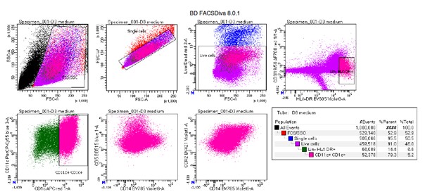
Author response figure 1: Manual gating example of human CD34-HPC derived DCs shows substantial autofluorescence.
Line 256: The hypothesis that the loss of CD36+CX3CR1+ cells was due to migration to the eye doesn't make sense based on volume and number of cells. 0.1% of all PBMC is ~1x10⁷ cells, and distributed throughout the eye would give about 1.3x10⁶ cells/mL of eye volume. This would make the eye turbid which is not consistent with birdshot chorioretinopathy and would be rare in HLA-B27 anterior uveitis and intermediate uveitis
We agree with the reviewer and have changed this in the manuscript section to “We speculated that the decrease in blood CD36+CX3CR1+ CD1c+ DCs was in part the result of migration of these cells to peripheral tissues (lymph nodes) and that these cells may also infiltrate the eye during active uveitis.” On page 17.
Line 267: Would have liked to see the gating of CX3CR1/CD36 cells be more consistent (there are overlapping CX3CR1+ and CX3CR1- populations in 5A, but in Figure 4 quadrants were used to define the populations when evaluating the numbers in uveitis and healthy controls. The populations in Figure 5 are more separated by CD36.
We agree with the reviewer and have added a more detailed example of the gating strategy used to sort CD36/CX3CR1 subsets in Figure 5 – Supplement 1 including the expression of CX3CR1 and CD36 in the sorted populations.
Line 269, IN VITRO stimulation: The experimental paradigm is set up to find a difference between cells but does not to test any biologically relevant scenario. By sorting on a surface marker, then stimulating with the ligand for that receptor, the result better proves that CD36 is important in TLR2 signaling than does it give any information on how these dendritic cells might behave in uveitis.
We agree with the reviewer that the connection between the cytokine expression of the CD1c+ subsets and non-infectious uveitis may benefit from additional experimental data. To this end, we profiled available eye fluid biopsies and paired plasma by Olink proteomics to measure 92 immune mediators from patients and controls from this study (and several additional samples, including aqueous humor from non-inflammatory cataract controls – see revised Figure 5 panel D). This analysis shows that cytokines produced by CD36+CX3CR1+ DCs such as TNF-alpha and IL-6 are specifically increased in eye tissue of patients, but not in blood. We hope the reviewer agrees that we have provided additional experimental data that links the functional differences in DC subsets to cytokines implicated in the pathogenesis of non-infectious uveitis.
Reviewer #3 (Public Review):
First, a note on nomenclature. The authors use the term 'auto-immune' uveitis to encapsulate three different conditions -- HLA-B27 anterior uveitis, idiopathic intermediate uveitis, and birdshot choroidopathy. While I would agree with this terminology for the third set, there is substantial controversy as to whether HLA-B27 is truly autoimmune or autoinflammatory. Indeed, one major hypothesis is that this condition is driven by changes in gut microbiome. Intermediate uveitis is even more problematic; a substantial number of cases of this condition will turn out to be associated with demyelinating disease, which has recently been linked to Epstein Barr virus disease. To my knowledge in none of these diseases has a definitive autoantigen been identified nor passive transfer via transfusion shown; I would suggest the authors abandon this terminology and simply refer to the conditions as they are called.
We would like to thank the reviewer for the constructive suggestions. We agree and have changed the term “autoimmune uveitis” to “non-infectious uveitis” throughout the manuscript.
Further, it would have been very desirable to compare the DC transcriptome for the other class of uveitic disease -- infectious -- for acute retinal necrosis or similar. As well it would have been very useful to compare profiles to other, related immune-mediated diseases such as ankylosing spondylitis.
We agree with the reviewer that comparison of DC transcriptomes is useful for interpretation of biological mechanisms involved. This is precisely the reason we use (in Figure 3) comparison of our DC transcriptomic data to well-controlled transgenic models and DC culture systems. This revealed NOTCH2-RUNX3 signaling driving the uveitis-associated CD1c+ DC signature. We have now included transcriptomic data from CD1c+ DC subsets of type I IFN diseases SLE and Systemic Sclerosis in Figure 2. Although we agree that comparison to infectious uveitis would be interesting, bulk RNA-seq data from CD1c+ DCs are – to the best of our knowledge – unfortunately not available.
Finally, it must be noted that looking for systemic signals in dendritic gene expression may be a bit of a needle in the haystack approach. Presumably, the function of the dendritic cells in uveitis is largely centered on those cells in the eye. It would have been highly desirable to examine the expression profile of intraocular DCs in at least a subset of patients who may have come to surgery (for instance, steroid implantation or vitrectomy).
We agree with the reviewer that analysis of blood requires enormous efforts and controls to dissect disease-relevant changes in gene profiles of cDC2 subsets. We therefore designed a strategy that focusses on replication of gene modules, use independent cohorts, and complementary immunophenotyping technologies to detect key changes in specific subsets of CD1c+ DCs in uveitis patients. To further extend these analyses, we have now also detailed our analysis of intraocular DCs using single-cell RNA seq of eye fluid biopsies (aqueous humor) of HLA-B27 anterior uveitis (identical to our “AU” group of patients). As shown in revised Figure 6, we detected eye-infiltrating CD1c+ DCs and were able to cluster cells positive for the uveitis-associated black module (revised Figure 6B), which showed – as expected - that “black-module+” CD1c+ DCs show higher expression for CD36, CX3CR1, and lower RUNX3, but not CD14 (revised Figure 6C)– closely corroborating our blood CD1c+ DC analyses. These DC3s were also found at higher frequency in the eye of patients with AU (Figure 6D). We hope the reviewer agrees we have sustainably improved the analysis of intraocular DCs and that this has now been sufficiently addressed.
It is also problematic that no effort has been made to assess the severity of uveitis. Flares of disease can range from extremely mild to debilitating. Similarly, intermediate uveitis and BSCR can range greatly in severity. Without normalizing for disease severity it is difficult to fully understand the range of transcriptional changes between cases.
In our view, a key limitation in determination of uveitis severity for molecular analysis is the fact that objective biomarkers that assess disease severity across uveitis entities are lacking. Currently, disease severity is dependent an array of clinical features (i.e, SUN criteria) which cannot be applied consistently to anterior, intermediate and posterior uveitis. For example, the severity of anterior uveitis is in part assessed by grading of inflammation in the anterior chamber, while the anterior chamber is (typically) not involved in Birdshot Uveitis (BU in this study). However, to allow the study of patients with high disease activity, we exclusively used systemic treatment-free patients that all had active uveitis at sampling at our academic institute, making the results highly relevant for understanding the pathophysiology of non-infectious uveitis. For this reviewer’s convenience, we have conducted additional analysis that includes key clinical parameters (anterior chamber cells, vitreous cells, and macular thickness for patients from cohort I). These data showed no clear clustering of patients based on any of the clinical parameters (revised Figure 1 -Supplement 2). We hope the reviewer agrees this has been addressed in sufficient detail.
The use of principal component analysis for clustering may be underpowered; I would suggest the authors apply UMAP to determine if higher dimensional component analyses correlate with disease type.
Upon request of the reviewer, we have conducted UMAP (with different tuning of hyperparameters) on the DEGs (cohort I, see image below). We believe that UMAP analysis did not provide additional insights or correlates with disease type. We hope the reviewer agrees.
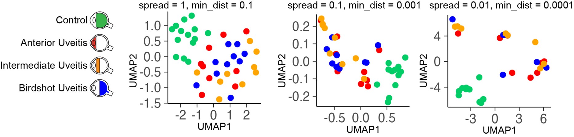
The false-discovery rate in large transcriptomic projects is challenging. While the authors are to be commended for employing a validation set, it would be useful to employ a Monte Carlo simulation in which groups are arbitrarily relabeled to determine the number of expected false discoveries within this data set (i.e. akin to Significance Analysis of Microarray techniques).
We determined the adjusted P values via the DESeq2 package (for false-discovery rate of 5% and Benjamini-Hochberg Procedure). The results are shown in Supplemental File 1K-1M and analysis in Figure 1A.
I do not fully understand the significance of the mouse CD11c-Runx3delta mice. It appears these data were derived from previous datasets or from bone marrow stromal line cultures. Did the authors attempt to generate autoimmune uveitis (i.e. EAU) in these animals? Without this the relevance for uveitis is unclear.
We did not attempt to induce experimental autoimmune uveitis in CD11c-Runx3delta mice. We used transcriptomic data from dendritic cells purified from this model to show that loss of RUNX3 induces a gene signature highly reminiscent of the gene module identified in non-infectious uveitis patients. Using enrichment analysis, we show that the transcriptome of patients is highly enriched for this signature which indicates that the decreased RUNX3 observed in patients underlies the upregulation of CD36, CX3CR1 and other surface genes. In other words, we used data from transgenic models to dissect which of the altered transcription factors were driving this gene module and we identified the RUNX3-NOTCH2 axis as an important contributor.
Author Response
We thank the reviewers for their positive feedback and thoughtful suggestions that will improve our manuscript. Here we summarise our plan for immediate action. We will resubmit our manuscript once additional experiments have been performed to clarify all the major and minor concerns of the reviewers and the manuscript has been revised. At that point, we will respond to all reviewer’s points and highlight the changes made in the text.
Reviewer #1 (Public Review):
The authors have tried to correlate changes in the cellular environment by means of altering temperature, the expression of key cellular factors involved in the viral replication cycle, and small molecules known to affect key viral protein-protein interactions with some physical properties of the liquid condensates of viral origin. The ideas and experiments are extremely interesting as they provide a framework to study viral replication and assembly from a thermodynamic point of view in live cells.
The major strengths of this article are the extremely thoughtful and detailed experimental approach; although this data collection and analysis are most likely extremely time-consuming, the techniques used here are so simple that the main goal and idea of the article become elegant. A second major strength is that in other to understand some of the physicochemical properties of the viral liquid inclusion, they used stimuli that have been very well studied, and thus one can really focus on a relatively easy interpretation of most of the data presented here.
There are three major weaknesses in this article. The way it is written, especially at the beginning, is extremely confusing. First, I would suggest authors should check and review extensively for improvements to the use of English. In particular, the abstract and introduction are extremely hard to understand. Second, in the abstract and introduction, the authors use terms such as "hardening", "perturbing the type/strength of interactions", "stabilization", and "material properties", for just citing some terms. It is clear that the authors do know exactly what they are referring to, but the definitions come so late in the text that it all becomes confusing. The second major weakness is that there is a lack of deep discussion of the physical meaning of some of the measured parameters like "C dense vs inclusion", and "nuclear density and supersaturation". There is a need to explain further the physical consequences of all the graphs. Most of them are discussed in a very superficial manner. The third major weakness is a lack of analysis of phase separations. Some of their data suggest phase transition and/or phase separation, thus, a more in-deep analysis is required. For example, could they calculate the change of entropy and enthalpy of some of these processes? Could they find some boundaries for these transitions between the "hard" (whatever that means) and the liquid?
The authors have achieved almost all their goals, with the caveat of the third weakness I mentioned before. Their work presented in this article is of significant interest and can become extremely important if a more detailed analysis of the thermodynamics parameters is assessed and a better description of the physical phenomenon is provided.
We thank reviewer 1 for the comments and, in particular, for being so positive regarding the strengths of our manuscript and for raising concerns that will surely improve the manuscript. At this point, we propose the following actions to address the concerns of Reviewer 1:
1) We will extensively revise the use of English, particularly, in the abstract and introduction, defining key terms as they come along in the text to make the argument clearer.
2) We acknowledge the importance of discussing our data in more detail and we propose the following. We will discuss the graphs and what they mean as exemplified in the paragraph below.
Regarding Figure 3 - As the concentration of vRNPs increases, we observe an increase in supersaturation until 12hpi. This means that contrary to what is observed in a binary mixture, in which the Cdilute is constant (Klosin et al., 2020), the Cdilute in our system increases with concentration. It has been reported that Cdilute increases in a multi-component system with bulk concentration (Riback et al., 2020). Our findings have important implications for how we think about the condensates formed during influenza infection. As the 8 different genomic vRNPs have a similar overall structure, they could, in theory, behave as a binary system between units of vRNPs and Rab11a. However, a change in Cdilute with concentration shows that our system behaves as a multi-component system. This means that the differences in length, RNA sequence and valency that each vRNP have are key for the integrity of condensates.
3) The reviewer calls our attention to the lack of analysis of phase separations. We think that phase separation (or percolation coupled to phase separation) governs the formation of influenza A virus condensates. However, we think we ought to exert caution at this point as the condensates we are working with are very complex and that the physics of our system in cells may not be sufficient to claim phase separation without an in vitro reconstitution system. In fact, IAV inclusions contain cellular membranes, different vRNPs and Rab11a. So far, we can only speculate that the liquid character of IAV inclusions may arise from a network of interacting vRNPs that bridge several cognate vRNP-Rab11 units on flexible membranes, similarly to what happens in phase separated vesicles in neurological synapses. However, the speculative model for our system, although being supported by correlative light and electron microscopy, currently lacks formal experimental validation.
For this reason, we thought of developing the current work as an alternative to explore the importance of the liquid material properties of IAV inclusions. By finding an efficient method to alter the material properties of IAV inclusions, we provide proof of principle that it is possible to impose controlled phase transitions that reduce the dynamics of vRNPs in cells and negatively impact progeny virion production. Despite having discussed these issues in the limitations of the study, we will make our point clearer.
We are currently establishing an in vitro reconstitution system to formally demonstrate, in an independent publication, that IAV inclusions are formed by phase separation. For this future work, we teamed up with Pablo Sartori, a theorical physicist to derive in- depth analysis of the thermodynamics of the viral liquid condensates. Collectively, we think that cells have too many variables to derive meaningful physics parameters (such as entropy and enthalpy) as well as models and need to be complemented by in vitro systems. For example, increasing the concentration inside a cell is not a simple endeavour as it relies on cellular pathways to deliver material to a specific place. At the same time, the 8 vRNPs, as mentioned above, have different size, valency and RNA sequence and can behave very differently in the formation of condensates and maintenance of their material properties. Ideally, they should be analysed individually or in selected combinations. For the future, we will combine data from in vitro reconstitution systems and cells to address this very important point raised by the reviewer.
From the paper on the section Limitations of the study: “Understanding condensate biology in living cells is physiologically relevant but complex because the systems are heterotypic and away from equilibria. This is especially challenging for influenza A liquid inclusions that are formed by 8 different vRNP complexes, which although sharing the same structure, vary in length, valency, and RNA sequence. In addition, liquid inclusions result from an incompletely understood interactome where vRNPs engage in multiple and distinct intersegment interactions bridging cognate vRNP-Rab11 units on flexible membranes (Chou et al., 2013; Gavazzi et al., 2013; Haralampiev et al., 2020; Le Sage et al., 2020; Shafiuddin & Boon, 2019; Sugita, Sagara, Noda, & Kawaoka, 2013). At present, we lack an in vitro reconstitution system to understand the underlying mechanism governing demixing of vRNP-Rab11a-host membranes from the cytosol. This in vitro system would be useful to explore how the different segments independently modulate the material properties of inclusions, explore if condensates are sites of IAV genome assembly, determine thermodynamic values, thresholds accurately, perform rheological measurements for viscosity and elasticity and validate our findings”.
Reviewer #2 (Public Review):
During Influenza virus infection, newly synthesized viral ribonucleoproteins (vRNPs) form cytosolic condensates, postulated as viral genome assembly sites and having liquid properties. vRNP accumulation in liquid viral inclusions requires its association with the cellular protein Rab11a directly via the viral polymerase subunit PB2. Etibor et al. investigate and compare the contributions of entropy, concentration, and valency/strength/type of interactions, on the properties of the vRNP condensates. For this, they subjected infected cells to the following perturbations: temperature variation (4, 37, and 42{degree sign}C), the concentration of viral inclusion drivers (vRNPs and Rab11a), and the number or strength of interactions between vRNPs using nucleozin a well-characterized vRNP sticker. Lowering the temperature (i.e. decreasing the entropic contribution) leads to a mild growth of condensates that does not significantly impact their stability. Altering the concentration of drivers of IAV inclusions impact their size but not their material properties. The most spectacular effect on condensates was observed using nucleozin. The drug dramatically stabilizes vRNP inclusions acting as a condensate hardener. Using a mouse model of influenza infection, the authors provide evidence that the activity of nucleozin is retained in vivo. Finally, using a mass spectrometry approach, they show that the drug affects vRNP solubility in a Rab11a-dependent manner without altering the host proteome profile.
The data are compelling and support the idea that drugs that affect the material properties of viral condensates could constitute a new family of antiviral molecules as already described for the respiratory syncytial virus (Risso Ballester et al. Nature. 2021).
Nevertheless, there are some limitations in the study. Several of them are mentioned in a dedicated paragraph at the end of a discussion. This includes the heterogeneity of the system (vRNP of different sizes, interactions between viral and cellular partners far from being understood), which is far from equilibrium, and the absence of minimal in vitro systems that would be useful to further characterize the thermodynamic and the material properties of the condensates.
We thank reviewer 2 for highlighting specific details that need improving and raising such interesting questions to validate our findings. We will address all the minor comments of Reviewer 2. To address the comments of Reviewer 2, we propose the actions described in blue below each point raised that is written in italics.
1) The concentrations are mostly evaluated using antibodies. This may be correct for Cdilute. However, measurement of Cdense should be viewed with caution as the antibodies may have some difficulty accessing the inner of the condensates (as already shown in other systems), and this access may depend on some condensate properties (which may evolve along the infection). This might induce artifactual trends in some graphs (as seen in panel 2c), which could, in turn, affect the calculation of some thermodynamic parameters.
The concern of using antibodies to calculate Cdense is valid. We will address this concern by validating our results using a fluorescent tagged virus that has mNeon Green fused to the viral polymerase PA (PA-mNeonGreen PR8 virus). Like NP, PA is a component of vRNPs and labels viral inclusions, colocalising with Rab11 when vRNPs are in the cytosol without the need of using antibodies.
This virus would be the best to evaluate inclusion thermodynamics, where it not an attenuated virus (Figure 1A below) with a delayed infection as demonstrated by the reduced levels of viral proteins (Figure 1B below). Consistently, it shows differences in the accumulation of vRNPs in the cytosol and viral inclusions form later in infection. After their emergence, inclusions behave as in the wild-type virus (PR8-WT), fusing and dividing (Figure 1C below) and displaying liquid properties. The differences in concentration may shift or alter thermodynamic parameters such as time of nucleation, nucleation density, inclusion maturation rate, Cdense, Cdilute. This is the reason why we performed the thermodynamics profiling using antibodies upon PR8-WT infection. For validating our results, and taking into account a possible delayed kinetics, and differenced that may occur because of reduced vRNP accumulation in the cytosol, this virus will be useful and therefore we will repeat the thermodynamics using it.
As a side note, vRNPs are composed of viral RNA coated with several molecules of NP and each vRNP also contains 1 copy of the trimeric RNA dependent RNA polymerase formed by PA, PB1 and PB2. It is well documented that in the cytosol the vast majority of PA (and other components of the polymerase) is in the form of vRNPs (Avilov, Moisy, Munier, et al., 2012; Avilov, Moisy, Naffakh, & Cusack, 2012; Bhagwat et al., 2020; Lakdawala et al., 2014), and thus we can use this virus to label vRNPs on condensates to corroborate our studies using antibodies.
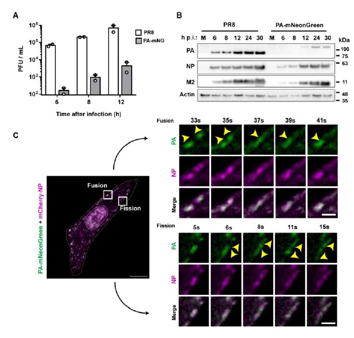
Figure 1 – The PA- mNeonGreen virus is attenuated in comparison to the WT virus. A. Cells (A549) were infected or mock-infected with PR8 WT or PA- mNeonGreen (PA-mNG) viruses, at a multiplicity of infection (MOI) of 3, for the indicated times. Viral production was determined by plaque assay and plotted as plaque forming units (PFU) per milliliter (mL) ± standard error of the mean (SEM). Data are a pool from 2 independent experiments. B. The levels of viral PA, NP and M2 proteins and actin in cell lysates at the indicated time points were determined by western blotting. C. Cells (A549) were transfected with a plasmid encoding mCherry-NP and co-infected with PA-mNeonGreen virus for 16h, at an MOI of 10. Cells were imaged under time-lapse conditions starting at 16 hpi. White boxes highlight vRNPs/viral inclusions in the cytoplasm in the individual frames. The dashed white and yellow lines mark the cell nucleus and the cell periphery, respectively. The yellow arrows indicate the fission/fusion events and movement of vRNPs/ viral inclusions. Bar = 10 µm. Bar in insets = 2 µm.
2) Although the authors have demonstrated that vRNP condensates exhibit several key characteristics of liquid condensates (they fuse and divide, they dissolve upon hypotonic shock or upon incubation with 1,6-hexanediol, FRAP experiments are consistent with a liquid nature), their aspect ratio (with a median above 1.4) is much higher than the aspect ratio observed for other cellular or viral liquid compartments. This is intriguing and might be discussed.
IAV inclusions have been shown to interact with microtubules and the endoplasmic reticulum, that confers movement, and also undergo fusion and fission events. We propose that these interactions and movement impose strength and deform inclusions making them less spherical. To validate this assumption, we compared the aspect ratio of viral inclusions in the absence and presence of nocodazole (that abrogates microtubule-based movement). The data in figure 2 shows that in the presence of nocodazole, the aspect ratio decreases from 1.42±0.36 to 1.26 ±0.17, supporting our assumption.
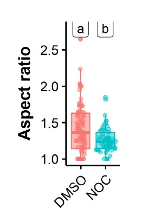
Figure 2 – Treatment with nocodazole reduces the aspect ratio of influenza A virus inclusions. Cells (A549) were infected PR8 WT and treated with nocodazole (10 µg/mL) for 2h time after which the movement of influenza A virus inclusions was captured by live cell imaging. Viral inclusions were segmented, and the aspect ratio measured by imageJ, analysed and plotted in R.
3) Similarly, the fusion event presented at the bottom of figure 3I is dubious. It might as well be an aggregation of condensates without fusion.
We will change this, thank you for the suggestion.
4) The authors could have more systematically performed FRAP/FLAPh experiments on cells expressing fluorescent versions of both NP and Rab11a to investigate the influence of condensate size, time after infection, or global concentrations of Rab11a in the cell (using the total fluorescence of overexpressed GFP-Rab11a as a proxy) on condensate properties.
We will try our best to be able to comply with this suggestion as we think it is important.
Reviewer #3 (Public Review):
This study aims to define the factors that regulate the material properties of the viral inclusion bodies of influenza A virus (IAV). In a cellular model, it shows that the material properties were not affected by lowering the temperature nor by altering the concentration of the factors that drive their formation. Impressively, the study shows that IAV inclusions may be hardened by targeting vRNP interactions via the known pharmacological modulator (also an IAV antiviral), nucleozin, both in vitro and in vivo. The study employs current state-of-the-art methodology in both influenza virology and condensate biology, and the conclusions are well-supported by data and proper data analysis. This study is an important starting point for understanding how to pharmacologically modulate the material properties of IAV viral inclusion bodies.
We thank this reviewer for all the positive comments. We will address the minor issues brought to our attention entirely, including changing the tittle of the manuscript and we will investigate the formation and material properties of IAV inclusions in the presence and absence of nucleozin for the nucleozin escape mutant NP-Y289H.
References
Avilov, S. V., Moisy, D., Munier, S., Schraidt, O., Naffakh, N., & Cusack, S. (2012). Replication- competent influenza A virus that encodes a split-green fluorescent protein-tagged PB2 polymerase subunit allows live-cell imaging of the virus life cycle. J Virol, 86(3), 1433- 1448. doi:10.1128/JVI.05820-11
Avilov, S. V., Moisy, D., Naffakh, N., & Cusack, S. (2012). Influenza A virus progeny vRNP trafficking in live infected cells studied with the virus-encoded fluorescently tagged PB2 protein. Vaccine, 30(51), 7411-7417. doi:10.1016/j.vaccine.2012.09.077
Bhagwat, A. R., Le Sage, V., Nturibi, E., Kulej, K., Jones, J., Guo, M., . . . Lakdawala, S. S. (2020). Quantitative live cell imaging reveals influenza virus manipulation of Rab11A transport through reduced dynein association. Nat Commun, 11(1), 23. doi:10.1038/s41467-019-13838-3
Chou, Y. Y., Heaton, N. S., Gao, Q., Palese, P., Singer, R. H., & Lionnet, T. (2013). Colocalization of different influenza viral RNA segments in the cytoplasm before viral budding as shown by single-molecule sensitivity FISH analysis. PLoS Pathog, 9(5), e1003358. doi:10.1371/journal.ppat.1003358
Gavazzi, C., Yver, M., Isel, C., Smyth, R. P., Rosa-Calatrava, M., Lina, B., . . . Marquet, R. (2013). A functional sequence-specific interaction between influenza A virus genomic RNA segments. Proc Natl Acad Sci U S A, 110(41), 16604-16609. doi:10.1073/pnas.1314419110
Haralampiev, I., Prisner, S., Nitzan, M., Schade, M., Jolmes, F., Schreiber, M., . . . Herrmann, A. (2020). Selective flexible packaging pathways of the segmented genome of influenza A virus. Nat Commun, 11(1), 4355. doi:10.1038/s41467-020-18108-1
Klosin, A., Oltsch, F., Harmon, T., Honigmann, A., Julicher, F., Hyman, A. A., & Zechner, C. (2020). Phase separation provides a mechanism to reduce noise in cells. Science, 367(6476), 464-468. doi:10.1126/science.aav6691
Lakdawala, S. S., Wu, Y., Wawrzusin, P., Kabat, J., Broadbent, A. J., Lamirande, E. W., . . . Subbarao, K. (2014). Influenza a virus assembly intermediates fuse in the cytoplasm. PLoS Pathog, 10(3), e1003971. doi:10.1371/journal.ppat.1003971
Le Sage, V., Kanarek, J. P., Snyder, D. J., Cooper, V. S., Lakdawala, S. S., & Lee, N. (2020). Mapping of Influenza Virus RNA-RNA Interactions Reveals a Flexible Network. Cell Rep, 31(13), 107823. doi:10.1016/j.celrep.2020.107823
Riback, J. A., Zhu, L., Ferrolino, M. C., Tolbert, M., Mitrea, D. M., Sanders, D. W., . . . Brangwynne, C. P. (2020). Composition-dependent thermodynamics of intracellular phase separation. Nature, 581(7807), 209-214. doi:10.1038/s41586-020-2256-2
Shafiuddin, M., & Boon, A. C. M. (2019). RNA Sequence Features Are at the Core of Influenza a Virus Genome Packaging. J Mol Biol. doi:10.1016/j.jmb.2019.03.018
Sugita, Y., Sagara, H., Noda, T., & Kawaoka, Y. (2013). Configuration of viral ribonucleoprotein complexes within the influenza A virion. J Virol, 87(23), 12879- 12884. doi:10.1128/JVI.02096-13
Author Response
Reviewer #2 (Public Review):
1) The main limitation of this study is that the results are primarily descriptive in nature, and thus, do not provide mechanistic insight into how Ryr1 disease mutations lead to the muscle-specific changes observed in the EDL, soleus and EOM proteomes.
An intrinsic feature of the high-throughput proteomic analysis technology is the generation of lists of differentially expressed proteins (DEP) in different muscles from WT and mutated mice. Although the definition of mechanistic insights related to changes of dozens of proteins is very interesting, it is a difficult task to accomplish and goes beyond the goal of the high-throughput proteomic analysis presented here. Nevertheless, the analysis of DEPs may indeed provide arguments to speculate on the pathogenesis of the phenotype linked to recessive RyR1 mutations. In the unrevised manuscript, we pointed out that the fiber type I predominance observed in congenital myopathies linked to recessive Ryr1 mutation are consistent with the high expression level of heat shock proteins in slow twitch muscles. However, as suggested by Reviewer 3, we have removed "vague statements" from the text of the revised manuscript, concerning major insights into pathophysiological mechanisms, since we are aware that the mechanistic information, if any, that we can extract from the data set, cannot go over the intrinsic limitation of the high-throughput proteomic technology.
b) Results comparing fast twitch (EDL) and slow twitch (soleus) muscles from WT mice confirmed several known differences between the two muscle types. Similar analyses between EOM/EDL and EOM/soleus muscles from WT mice were not conducted.
We agree with the point raised by the Reviewer. In the revised manuscript we have changed Figure 2. The new Figure 2 shows the analysis of differentially expressed proteins in EDL, soleus and EOMs from WT mice. We have also added 2 new Tables (new Supplementary Table 2 and 3) and have inserted our findings in the revised Results section (page, 7, lines 157-176, pages 8 and 9).
c) While a reactome pathway analysis for proteins changes observed in EDL is shown in Supplemental Figure 1, the authors do not fully discuss the nature of the proteins and corresponding pathways impacted in the other two muscle groups analyzed.
We have now included in the revised manuscript a new Figure 2 which includes the Reactome pathway analysis comparing EDL with soleus, EDL with EOM and soleus with EOM (panels C, F and I, respectively). We have also inserted into the revised manuscript a brief description of the pathways showing the greatest changes in protein content (page 7 line 156-175, pages 8 and 9). We agree that the data showing changes in protein content between the 3 muscle groups of the WT mice are important also because they validate the results of the proteomic approach. Indeed, the present results confirm that many proteins including MyHCIIb, calsequestrin 1, SERCA1, parvalbumin etc are more abundantly expressed in fast twitch EDL muscles compared to soleus. Similarly, our results confirm that EOMs are enriched in MyHC-EO as well as cardiac isoforms of ECC proteins. This point has been clarified in the revised version of the manuscript (page 8, lines 198-213; page 9 lines 214-228). Nevertheless, we would like to point out that the main focus of our study is to compare the changes of protein content induced by the presence of recessive RyR1 mutations.
Reviewer #3 (Public Review):
a) it would be useful to determine whether changes in protein levels correlated with changes in mRNA levels …….
We performed qPCR analysis of Stac3 and Cacna1s in EDL, Soleus and EOM from WT mice (see Figure 1 below). The expression of transcripts encoding Cacna1s and Stac3 is approximately 9-fold higher in EDL compared to Soleus. The fold change of Stac3 and Cacna1s transcripts in EDL muscles is higher compared to the differences we observed by Mass spectrometry at the protein level between EDL and Soleus. Indeed, we found that the content of the Stac3 protein in EDL is 3-fold higher compared to that in soleus. Although there is no apparent linear correlation between mRNA and protein levels, we believe that a few plausible conclusions can be drawn, namely: (i) the expression level of both transcripts and proteins is higher EDL compared to EOM and soleus muscles, respectively, (ii) the expression level of transcripts encoding Stac3 correlate with those encoding Cacan1s and confirm proteomic data. In addition, the level of Stac3 transcript does not changes between WT and dHT, confirming our proteomic data which show that Stac3 protein content in muscles from dHT is similar to that found in WT littermates. Altogether these results support the concept that the differences in Stac3 content between EDL and soleus occur at both the protein and transcript levels, namely high Stac3 mRNA level correlates with higher protein content (EDL) and low mRNA levels correlated with low Stac3 protein content in Soleus muscles (see Figure 1 below).
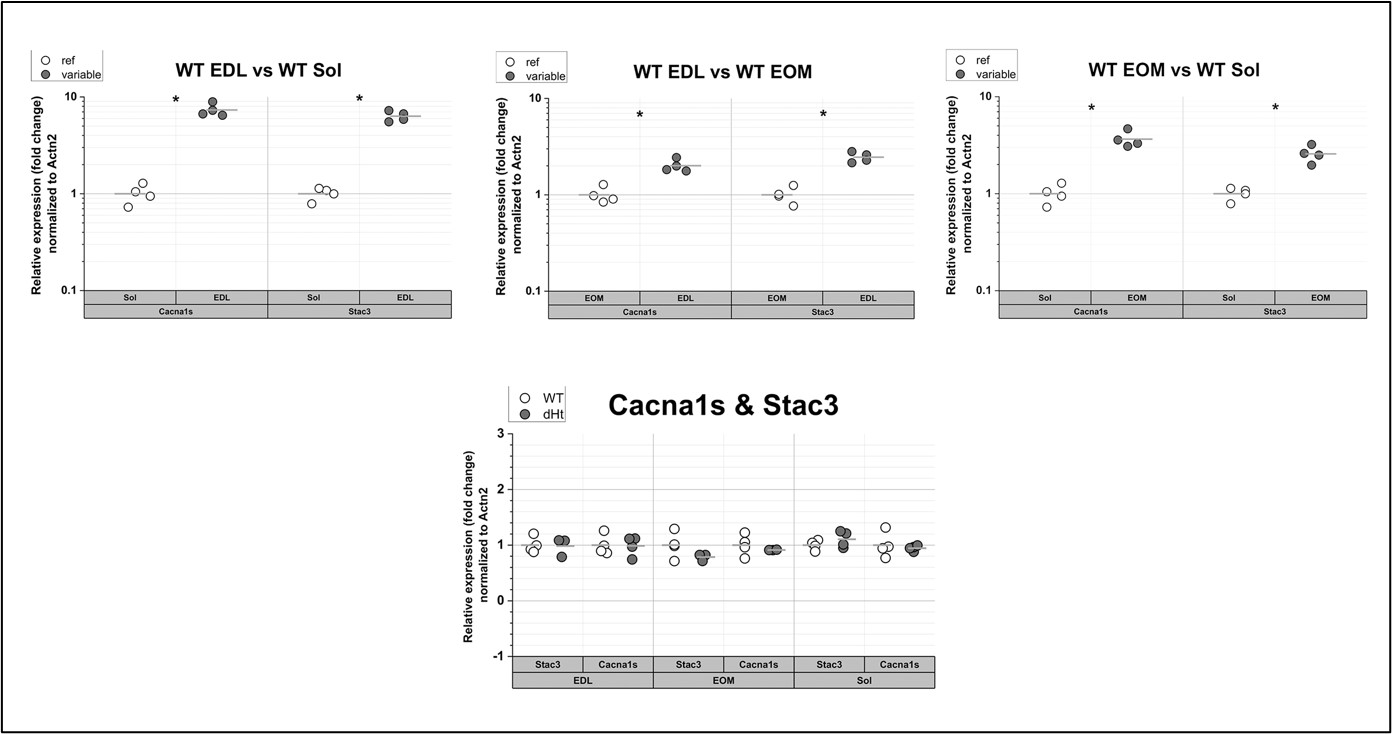
Figure 2: qPCR of Cacna1s and Stac3 in muscles from WT mice. The expression levels of the transcripts encoding Cacna1s and Stac3 are the highest in EDL muscles and the lowest in soleus muscles (top panels). There are no significant changes in their relative expression levels in dHT vs WT. Each symbol represents the value from of a single mouse. * p=0.028 Mann Whitney test qPCR was performed as described in Elbaz et al., 2019 (Hum Mol Genet 28, 2987-2999).
….and whether or not the protein present was functional, and whether Stac3 was in fact stoichiometrically depleted in relation to Cacna1s.
We thought about this point but think that there are no plausible arguments to believe that Stac3 is not functional, one simple reason being that our WT mice do not have a phenotype which would be associated with the absence of Stac3 (Reinholt et al., PLoS One 8, e62760 2013, Nelson et al. Proc. Natl. Acad. Sci. USA 110:11881 2013).
b) In the abstract, the authors stated that skeletal muscle is responsible for voluntary movement. It is also responsible for non-voluntary. The abstract needs to be refocused on the mutation and on what we learn from this study. Please avoid vague statements like "we provide important insights to the pathophysiological mechanisms..." mainly when the study is descriptive and not mechanistic.
The abstract of the revised manuscript has been rewritten. In particular, we removed statements referring to important “pathophysiological mechanistic insight”.
c) The author should bring up the mutation name, location and phenotype early in the introduction.
In the revised manuscript we provide the information requested by the Reviewer (page 2 lines 36-38 and page 4, lines 98-102).
d) This reviewer also suggests that the authors refocus the introduction on the mutation location in the 3D RyR1 structure (available cryo-EM structure), if there is any nearby ligand binding site, protomers junction or any other known interacting protein partners. This will help the reader to understand how this mutation could be important for the channel's function
The residue Ala4329 is present inside the TMx (Auxiliary transmembrane helices) domain which spans from residue 4322 to 4370 and interposes structurally (des Georges A et al. 2016 Cell 167,145-57; Chen W, et al. 2020 EMBO Rep. 21, e49891). Although the structural resolution of the region has been improved (des Georges et al, 2016), parts of the domain still remain with no defined atomic coordinates, especially the region encompassing a.a. E4253 – F4540. Because of such undefined atomic coordinates of the region E4253-F4540, we are not able to determine the real orientation and the disposition of the amino acids in this region, including the A4329 residue. As reference, structure PDB: 5TAL of des Georges et al, 2016 was analyzed with UCSF Chimera (production version 1.16) (Pettersen et al. J. Comput. Chem. 25: 1605-1612. doi: 10.1002/jcc.20084).
Author Response
Reviewer #1 (Public Review):
The authors reveal dual regulatory activity of the complex nuclear receptor element (cNRE; contains hexads A+B+C) in cardiac chambers and its evolutionary origin using computational and molecular approaches. Building upon a previous observation that hexads A and B act as ventricular repressor sequences, in this study the authors identify a novel hexad C sequence with preferential atrial expression. The authors also reveal that the cNRE emerged from an endogenous viral element using comparative genomic approaches. The strength of this study is in a combination of in silico evolutionary analyses with in vivo transgenic assays in both zebrafish and mouse models. Rapid, transient expression assays in zebrafish together with assays using stable, transgenic mice demonstrate dual functionality of cNRE depending on the chamber context. This is especially intriguing given that the cNRE is present only in Galliformes and has originated likely through viral infection. Interestingly, there seem to be some species-specific differences between zebrafish and mouse models in expression response to mutations within the cNRE. Taken together, these findings bear significant implications for our understanding of dual regulatory elements in the evolutionary context of organ formation.
We thank reviewer 1 for the thorough review and are very satisfied with his favorable view of our manuscript. We also thank reviewer 1 for suggestions and opportunities to further clarify some relevant issues.
Reviewer #2 (Public Review):
Nunes Santos et al. investigated the gene regulatory activity of the promoter of the quail myosin gene, SMyHC III, that is expressed specifically in the atria of the heart in quails. To do so, they computationally identified a novel 6-bp sequence within the promoter that is putatively bound by a nuclear receptor transcription factor, and hence is a putative regulatory sequence. They tested this sequence for regulatory activity using transgenic assays in zebrafish and mice, and subjected this sequence to mutagenesis to investigate whether gene regulatory effects are abrogated. They define this sequence, together with two additional known 6-bp regulatory sequences, as a novel regulatory sequence (denoted cNRE) necessary and sufficient for driving atrial-specific expression of SMyHC III. This cNRE sequence is shared across several galliform species but appears to be absent in other avian species. The authors find that there is sequence homology between the cNRE and several virus genomes, and they conclude that this regulatory sequence arose in the quail genome by viral integration.
Strengths: The evolutionary origins of gene regulatory sequences and their impact on directing tissue-specific expression are of great interest to geneticists and evolutionary biologists. The authors of this paper attempt to bring this evolutionary perspective to the developmental biology question of how genes are differentially expressed in different chambers of the heart. The authors test for regulatory activity of the putative regulatory sequence they identified computationally in both zebrafish and mouse transgenic assays. The authors disrupt this sequence using deletions and mutagenesis, and introduce a tandem repeat of the sequence to a reporter gene to determine its consequences on chamber activity. These experiments demonstrate that the identified sequence has regulatory activity.
We appreciate the thorough review of our manuscript and are very stimulated by the reviewer’s understanding of the contents we presented. We will take the liberty to comment after the reviewer’s considerations, in the hope to better answer the relevant points.
Weaknesses: There are several decisions and assumptions that have been made by the authors, the reasons for which have not been articulated. Firstly, the rationale for the approach is not clear. The study is a follow-up to work previously performed by the authors which identified two 6-bp sequences important for controlling atrial-specific expression of the quail SMyHC III gene. This study appears to be motivated by the fact that these two sequences, bound by nuclear receptors, do not fully direct chamber-specific expression, and therefore this study aims to find additional regulatory sequences. It is assumed that any additional regulatory sequences should also be bound by nuclear receptors, and be 6-bp in length, and therefore the authors search for 6-bp sequences bound by nuclear receptors. It is not clear what the input sequence for this analysis was.
Thank you for giving us the opportunity to clarify our rational. Our approach is justified by the natural progression in the understanding of the mechanisms involved in preferential atrial expression by the SMyHC III promoter. The groundwork was solidly laid down by Wang and colleagues (see references as below). They mapped potential atrial stimulators and ventricular repressors throughout the SMyHC III promoter using atrial and ventricular cultures, respectively. Wang and colleagues pinned down the relevant regulators. First between -840 and -680 bp upstream from the transcription start site, then inside this nucleotide stretch, then in the 72-bp fragment contained between -840 and -680 bp, then identified the ventricular repressor in Hexads A and B inside the 72-bp sequence (see references below). We, in this manuscript, contributed with the identification of Hexad C (immediately downstream of Hexads A and B) as a potential nuclear receptor binding site and as a bona fide atrial activator. In summary, our work represents a logical conclusion of previous work by Wang and colleagues. We continued the process of narrowing down sequences previously proven to contain atrial activators (that were unknown before our present work) and ventricular repressors (that were already described).
Why did we use nuclear receptors as models for the putative cardiac chamber regulators binding to the cNRE? This is because previous work by Wang et al., 1996, 1998, 2001 and by Bruneau et al., 2001 showed that the 5’ portion of the cNRE (Hexads A and B) is indeed a hub for the integration of signals conveyed by nuclear receptors. Originally, Wang et al., 1996 showed that the VDR response element is a ventricular repressor acting via the 5’ portion of the cNRE. In a subsequent manuscript, Wang et al., 1998 showed that both RAR and VDR bind the 5’ portion of the cNRE. Bruneau et al., 2001 showed, by crossing IRX4 knockout mice with SMyHC III-HAP mice (Xavier-Neto et al., 1999), that IRX4 plays the role of a repressor of SMyHC III-HAP expression. Finally, Wang et al., 2001 showed that IRX4 interacts with RXR bound to the 5’ portion of the cNRE to inhibit ventricular expression.
Why was the 3’ Hexad included as a research subject? Very early on in our work it was noted that 3’ of the original VDR response element (Hexads A and B), described by Wang et al., 1996 and 1998 as a ventricular repressor, there was a sequence (Hexad C) with almost equal binding potential to nuclear receptors as Hexads A and B (as initially judged on the basis of comparisons with canonical nuclear receptor binding sequences, but later on confirmed by in silico profiling of nuclear receptor binding, see below). This discovery prompted us to design point mutants in the 3’ portion of the cNRE to investigate whether Hexad C contained relevant regulators of heart chamber expression. These analyses revealed a strong atrial activator in the mouse (the missing atrial activator from Wang et al., 1996, 1998, 2001).
Wang, G. F., Nikovits, W., Schleinitz, M., and Stockdale, F. E. (1996). Atrial chamber-specific expression of the slow myosin heavy chain 3 gene in the embryonic heart. J. Biol. Chem. 271, 19836-19845.
Wang, G. F., Nikovits, W. Jr., Schleinitz, M., and Stockdale, F. E. (1998). A positive GATA element and a negative vitamin D receptorlike element control atrial chamber-specific expression of a slow myosin heavy-chain gene during cardiac morphogenesis. Mol. Cell Biol. 18, 6023-6034.
Xavier-Neto, J., Neville, C. M., Shapiro, M. D., Houghton, L., Wang, G. F., Nikovits, W. Jr, Stockdale, F. E., and Rosenthal, N. (1999). A retinoic acid-inducible transgenic marker of sino-atrial development in the mouse heart. Development 126, 2677-2687.
Bruneau, B. G., Bao, Z. Z., Fatkin, D., Xavier-Neto, J., Georgakopoulos, D., Maguire, C. T., Berul, C. I., Kass, D. A., Kuroski-de Bold, M. L., de Bold, A. J., Conner, D. A., Rosenthal, N., Cepko, C. L., Seidman, C. E., and Seidman, J. G. (2001). Cardiomyopathy in Irx4-deficient mice is preceded by abnormal ventricular gene expression. Mol. Cell Biol. 21, 1730-1736.
Wang, G. F., Nikovits, W. Jr., Bao, Z.Z., and Stockdale, F.E. (2001). Irx4 forms an inhibitory complex with the vitamin D and retinoic X receptors to regulate cardiac chamber-specific slow MyHC3 expression. J Biol Chem. 276, 28835-28841.
The methods section mentions the cNRE sequence, but this is their newly defined regulatory sequence based on the newly identified 6-bp sequence. It is therefore unclear why Hexad C was identified to be of interest, and not the GATA binding site for example, and whether other sequences in the promoter might have stronger effects on driving atrial-specific expression.
As far as the existence of binding sites other than Hexads A, B, and C, we cannot, formally, exclude the possibility that there may be other relevant regulators of the SMyHC III gene. But we note that the sequences that we utilized were previously mapped through deletion mutant promoter approach by Wang et al., 1996 as the most powerful atrial activator(s) and ventricular repressor(s). We addressed these concerns in a new session entitled “Limitations of our work”.
Concerning GATA regulation, Wang et al., 1996, 1998 characterized a GATA-4 site that drives generalized (atrial and ventricular) cardiac expression in quail cultures. However, we were unable to identify any relevant changes in cardiac expression in mutant GATA SMyHC III-HAP transgenic mouse lines produced with the same mutated promoter sequences described by Wang et al., 1996, 1998.
Finding Hexad C as an atrial activator was an experimental finding. We identified it as such because we had two important inputs. First, in 1997, we consulted with Ralff Ribeiro, a specialist on nuclear receptors and he pointed out that downstream of the Hexad A + Hexad B VDRE/RARE (the ventricular repressor), there was a sequence with good potential for a nuclear receptor binding motif. This was exactly Hexad C. Then, we confirmed its potential for nuclear receptor binding by nuclear receptor profiling. After these two pieces of evidence, we thought that there was enough evidence to justify a mutant construct (Mut C). The experimental results we obtained in transgenic mice and zebrafish are consistent with the hypothesis that Hexad C does contain the long sought atrial activator predicted by Wang et al., 1996 in atrial cultures. This seems to be the most important atrial activator (a seven-fold activator) predicted by a deletion approach to be located between -840 and 680 bp in Wang et al., 1996.
Wang, G. F., Nikovits, W., Schleinitz, M., and Stockdale, F. E. (1996). Atrial chamber-specific expression of the slow myosin heavy chain 3 gene in the embryonic heart. J. Biol. Chem. 271, 19836-19845.
Wang, G. F., Nikovits, W. Jr., Schleinitz, M., and Stockdale, F. E. (1998). A positive GATA element and a negative vitamin D receptorlike element control atrial chamber-specific expression of a slow myosin heavy-chain gene during cardiac morphogenesis. Mol. Cell Biol. 18, 6023-6034.
Indeed, the zebrafish transgenic assays use the 32 bp cNRE, while in the mouse transgenic assays, a 72 bp region is used. This choice of sequence length is not justified.
As stated above, our rational was built as a continuation of the thorough work by Wang and colleagues in progressively narrowing down the location of relevant atrial stimulators and ventricular repressors. Throughout our work, we sought to obtain maximal coherence with previous studies (see references below) and to simultaneously probe cNRE function at an increased resolution. For that, we utilized previously described mutant SMyHC III promoter constructs (Wang et al., 1996) and introduced novel site-directed dinucleotide substitution mutants of individual Hexads in the SMyHC III promoter.
Wang, G. F., Nikovits, W., Schleinitz, M., and Stockdale, F. E. (1996). Atrial chamber-specific expression of the slow myosin heavy chain 3 gene in the embryonic heart. J. Biol. Chem. 271, 19836-19845.
Wang, G. F., Nikovits, W. Jr., Schleinitz, M., and Stockdale, F. E. (1998). A positive GATA element and a negative vitamin D receptorlike element control atrial chamber-specific expression of a slow myosin heavy-chain gene during cardiac morphogenesis. Mol. Cell Biol. 18, 6023-6034.
Xavier-Neto, J., Neville, C. M., Shapiro, M. D., Houghton, L., Wang, G. F., Nikovits, W. Jr, Stockdale, F. E., and Rosenthal, N. (1999). A retinoic acid-inducible transgenic marker of sino-atrial development in the mouse heart. Development 126, 2677-2687.
Bruneau, B. G., Bao, Z. Z., Fatkin, D., Xavier-Neto, J., Georgakopoulos, D., Maguire, C. T., Berul, C. I., Kass, D. A., Kuroski-de Bold, M. L., de Bold, A. J., Conner, D. A., Rosenthal, N., Cepko, C. L., Seidman, C. E., and Seidman, J. G. (2001). Cardiomyopathy in Irx4-deficient mice is preceded by abnormal ventricular gene expression. Mol. Cell Biol. 21, 1730-1736.
Wang, G. F., Nikovits, W. Jr., Bao, Z.Z., and Stockdale, F.E. (2001). Irx4 forms an inhibitory complex with the vitamin D and retinoic X receptors to regulate cardiac chamber-specific slow MyHC3 expression. J Biol Chem. 276, 28835-28841.
The decisions about which bases to mutate in the three hexads are also not clear. Why are the first two bases mutated in Hexad B and C and the whole region mutated in Hexad A? Is there a reason to believe these bases are particularly important?
As for the reasons behind mutation of the first two bases in Hexad B and Hexad C, there were two:
One reason is because these point mutations in Hexads B and C were planned after the publication of Wang et al., 1996, which defined the major role of Hexad A in ventricular repression. After this discovery, we decided that a higher level of resolution in our mutation approach would be a better way to search for additional regulators of SMyHC III expression, including the atrial regulator that was readily apparent from the results shown in Wang et al., 1996, but had not yet been described.
The second reason is because the two first nucleotides (purines) in a nuclear-receptor binding hexad are critical for the interaction between target DNA and transcription factors of the nuclear receptor family. Substituting pyrimidines for purines in the two first positions of an hexad drastically reduces the affinity of a nuclear response element, and that is why we chose to use TT substitutions in our mutant constructs. Please refer to: Umesono et al., Cell, 1991 65: 12551266 for a review; Mader et al., J Biol Chem, 1993 268:591-600 for a mutation study; Rastinejad et al., EMBO J., 2000 19:1045-1054 for a crystallographic study (as well as additional references listed below).
Mader, S., Chen, J. Y., Chen, Z., White, J., Chambon, P., and Gronemeyer, H. (1993). The patterns of binding of RAR, RXR and TR homo- and heterodimers to direct repeats are dictated by the binding specificites of the DNA binding domains. EMBO J. 12, 50295041.
Ribeiro, R. C., Apriletti, J. W., Yen, P.M., Chin, W. W., and Baxter, J. D. (1994). Heterodimerization and deoxyribonucleic acid-binding properties of a retinoid X receptor-related factor. Endocrinology.135, 2076-2085.
Zhao, Q., Chasse, S. A., Devarakonda, S., Sierk, M. L., Ahvazi, B., and Rastinejad, F. (2000). Structural basis of RXR-DNA interactions. J. Mol. Biol. 296, 509-520.
Shaffer, P. L. and Gewirth, D. T. (2002). Structural basis of VDR-DNA interactions on direct repeat response elements. EMBO J. 21, 2242-2252.
The control mutant also has effects on the chamber distribution of GFP expression.
We note that, in the mouse, MutS did not produce any major changes from the typical wild type phenotypes linked to SMyHC III-HAP transgenic hearts. We concluded, based on our data, that the spacing mutant worked reasonably well as a negative mutation control in mice. We agree that it would have been particularly elegant if a spacing mutant designed for the mouse context worked in the exact same way in the zebrafish. However, the fact that there are slight differences in behavior for the mutated “spacing” constructs in species separated by, millions of years of independent evolution is not really surprising, given that the amino acid sequence of transcription factors can diverge and co-evolve with binding nucleotides and end up drifting quite substantially from an ancestral setup. As we reiterate below, we consider more fundamental the fact that the cNRE is actually able to bias cardiac expression towards a model of preferential atrial expression, even in the context of species separated by millions of years of independent evolution.
Two claims in the paper have weak evidence. Firstly, the conclusion that the cNRE is necessary and sufficient for driving preferential expression in the atrium. Deleting the cNRE does reduce the amount of atrial reporter gene expression but there is not a "conversion" from atrial to ventricular expression as mentioned in line 205. Similarly, a fusion of 5 tandem repeats of the cNRE can induce expression of a ventricular gene in the atria (I'm assuming a single copy is insufficient), but does not abolish ventricular expression.
We agree that our labelling of the cNRE is perhaps too strong, and we have toned it down accordingly to incorporate the much more equilibrated concept that the cNRE biases cardiac expression towards a model of preferential atrial expression.
However, after the corrections suggested, we believe our assertion is now justified. We show that in the mouse, removal of the cNRE is followed by a major reduction of atrial expression coupled to the release of a low, but quite clear level of expression in the ventricles, when compared to the transgenic mouse harboring the wild type SMyHC III promoter. Note that, as expected, the relative power of the cNRE to establish preferential atrial expression is higher in the mouse (a mammal) than it is in the zebrafish (a teleost), which is biologically sound, as mammals and avians are closer, phylogenetically, than teleosts and avians. Yet, the direction of change of expression in atria and ventricles was exactly as expected, if a given motif responsible for preferential atrial expression was removed (the cNRE in our case), that is: marked reduction in atrial expression and small (albeit clearly evident) release of ventricular expression. We believe that these directional changes observed in species separated by millions of years of independent evolution constitute very good biological evidence for the role of the cNRE in driving preferential atrial expression.
Concerning the 5x fusion of cNREs, we chose to produce this multimer for safety purposes only, because we did not want to risk performing incomplete experiments and having to repeat them. However, more to the point, we later compared the efficiency of one (1) versus five (5) cNRE copies in a cell culture context and the results were not different.
Secondly, the authors claim that the cNRE regulatory sequence arose from viral integration into the genomes of galliform species. While this is an attractive mechanism for explaining novel regulatory sequences, the evidence for this is based purely on sequence homology to viral genomes. And this single observation is not robust as the significance of the sequence matches does not appear to be adjusted for sequence matches expected by chance. The "evolutionary pathway" leading to the direction of chamber-specific expression in the heart as highlighted in the abstract has therefore not been demonstrated.
We agree with the reviewer. Because of space constraints, we decided to omit a substantial part of our work from the initial submission of the manuscript. We now include the relevant data in the revised version. We thus mapped the phylogenetic origins of the SMyHC III family of slow myosins and then established how and when the cNREs became topologically associated with the SMyHC III gene. To do that, we repeat masked all available sequences from avian SMyHC III orthologs. As it will become clear below, the cNRE is a rare sequence, rather than a low complexity repeat. Our search for cNREs outside of the quail context (Coturnix coturnix) followed two independent lines. First, we took a scaled, evolution-oriented approach. Initially, we looked for cNREs in species close to the quail (i.e., Galliformes) and then progressively farther, to include derived (i.e., Passeriformes) and basal avians (i.e., Paleognaths) as well as external groups such as crocodilians. While pursuing this line of investigation, it became clear that the cNRE was a rare form of repetitive element, which showed a conserved topological relationship with the SMyHC III gene (i.e., cNREs flanked the SMyHC III genes at 5’ and 3’ regions). Using this topological relationship as a character, we determined when it appeared during avian evolution and then set out to establish the likely origins of this rare repetitive motif. This search for the origins of the cNRE entailed comparisons to databases of repetitive genome elements, until the extreme telomeric nature of the SMyHC III gene became evident. This finding directed us to the fact that the hexad nature of the cNRE is reminiscent of the hexameric character of telomeric direct repeats. Because direct telomeric repeats are exactly featured in the genomes of avian DNA viruses that can infect the germline and integrate into the avian genome, we focused our search for the cNRE on the members of the subfamily Alphaherpesvirinae (Morissette & Flamand, 2010). In this search, we utilized the human herpes simplex virus 1 (HSV1) as a general model for herpes viruses, and a set of four (4) members of the Alphaherpesvirinae family that specifically infect Galliformes (i.e., GaHV1, the virus responsible for avian infectious laryngotracheitis in chicken, GaHV2, the Marek’s disease virus, GaHV3, a non-pathogenic virus, and MeHV1, the non-pathogenic Meleagrid herpesvirus 1 capable of infecting chicken and wild turkey) (Waidner et al., 2009). The search for cNREs in Alphaherpesvirinae was successful. We found six (6) cNRE hits in HSV1, one (1) in GaHV1, and none in MeHV1, GaHV2, and GaHV3. Our evolution-directed approach thus led to the direct recognition that cNREs can be found in the genomes of a family of viruses that contain members that infect avians and integrate their double-stranded DNA into the host germline (Morissette & Flamand, 2010). Therefore, as a second independent approach, as pointed out by the reviewer, we set out to further extend this proof of concept by broadening our search to all known sequenced viruses and perform an unbiased, internally consistent, and quantitative analysis of cNRE presence in viral genomes, as already reported in the initial submission of this manuscript.
Reviewer #3 (Public Review):
Summary:
In this manuscript Nunes Santos et al. use a combination of computation and experimental methods to identify and characterize a cis-regulatory element that mediates expression of the quail Slow Myosin Heavy Chain III (SMyHC III) gene in the heart (specifically in the atria). Previous studies had identified a cis-regulatory element that can drive expression of SMyHC III in the heart, but not specifically (solely) in the atria, suggesting additional regulatory elements are responsible for the specific expression of SMyHC III in the atria as opposed to other elements of the heart. To identify these elements Nunes Santos et al. first used a bioinformatic approach to identify potentially functional nuclear receptor binding sites ("Hexads") in the SMyHC III promoter; previous studies had already shown that two of these Hexads are important for SMyHC III promoter function. They identified a previously unknown third Hexad within the promoter, and propose that the combination of these three (called the complex Nuclear Receptor Element or cNRE) is necessary and sufficient for specific atrial expression of SMyHC III. Next, they use experimental methods to functionally characterize the cNRE including showing that the quail SMyHC III promoter can drive green fluorescent protein (GFP) expression the atrium of developing zebrafish embryos and that the cNRE is necessary to drive the expression of the human alkaline phosphatase reporter gene (HAP) in transgenic mouse atria. Additional experiments show that the cNRE is portable regulatory element that can drive atrial expression and demonstrate the importance of the three Hexad parts. These data demonstrating that the cNRE mediates atrial-specific expression is well-done and convincing. The authors also note the possibility that the cNRE might be derived from an endogenous viral element but further data are needed to support the hypothesis that the cNRE is of viral origin.
Strengths:
1) The experimental work demonstrating that the cNRE is a regulatory element that can mediate the atrial-specific expression of SMyHC III.
We thank reviewer 3 for this thorough appreciation of our work and are pleased with the evaluation of our manuscript’s potential.
Weaknesses:
1) Justification for use of different regulatory elements in the zebrafish (32 bp cNRE) and the mouse transgenic assays (72 bp cNRE), and discussion of the impact of this difference on the results/interpretation.
In general, throughout our work, we sought to obtain maximal coherence with previous studies (see references below) and to simultaneously probe cNRE function at an increased resolution. For that, we utilized previously described mutant SMyHC III promoter constructs (Wang et al., 1996, 1998) and introduced novel site-directed dinucleotide substitution mutants of individual Hexads in the SMyHC III promoter. Actually, the 72-bp construct is not a 72-bp construct. It is a 5’ deletion construct that removed 72 bp from the 840 bp wild type SMyHC III construct, transforming it into a 768-bp SMyHC III promoter construct. Any directional changes observed in cardiac expression by the 768 bp as compared to the wild type promoter was interpreted in the context as missing regulators present in this 5’ 72 bp.
Wang et al., 1996 and 1998 had already shown that Hexads A and B contained a functional VDRE/RARE, which acted as a ventricular repressor. Using the 768-bp SMyHC III promoter in mouse transgenic lines was thus a natural investigation step for us to evaluate whether regulation of the SMyHC III promoter in the mouse was similar in mice as compared to quail cardiac cultures. As shown in the manuscript, deletion of the 72 bp resulted in the release of a low level of expression in ventricles, consistent with the removal of a ventricular repressor (already described by Wang et al., 1996). It also showed a marked reduction in atrial transgene stimulation, suggesting the elimination of a very important atrial activator.
In 1996, Wang and colleagues mapped an atrial activator to the sequence interval of 160 bp, between -840 and -680 bp (Wang et al., 1996). In our mouse transgenics, we reduced this interval to a mere 72 bp, between -840 to -768 bp. This was very useful information. Wang et al., 1998 showed that HF-1a, M-CAT, and E-box sites located between -840 and -808 bp did not influence atrial expression, so now we had a potential interval of only 40 bp between -808 and -768 bp. Further, our transgenic mice indicated that the GATA site located 3’ from Hexads A, B, and C (GATA site changed to a Sal I site at positions -749 to -743 bp) did not work as a general activator, as in the quail. Thus, the only good candidate for the atrial activator in mice inside the 40-bp fragment between -808 and -768 bp was the cNRE, with its three Hexads, A, B and the novel Hexad C. Because Hexads A plus B composed a functional VDRE/RARE that played a role in ventricular repression in the quail, we hypothesized that the atrial activator would be present in Hexad C. We then mutated the two first purines in Hexad C (the most important ones for nuclear receptor binding, please refer to Umesono et al., Cell, 1991 65: 1255-1266 for a review; Mader et al., J Biol Chem, 1993 268:591-600 for a mutation study; Rastinejad et al., EMBO J., 2000 19:1045-1054 for a crystallographic study as well as additional references listed below) and performed the experiments that demonstrated a profound reduction in atrial expression in the mouse context, revealing the long-sought atrial activator.
Mader, S., Chen, J. Y., Chen, Z., White, J., Chambon, P., and Gronemeyer, H. (1993). The patterns of binding of RAR, RXR and TR homo- and heterodimers to direct repeats are dictated by the binding specificites of the DNA binding domains. EMBO J. 12, 50295041.
Ribeiro, R. C., Apriletti, J. W., Yen, P.M., Chin, W. W., and Baxter, J. D. (1994). Heterodimerization and deoxyribonucleic acid-binding properties of a retinoid X receptor-related factor. Endocrinology.135, 2076-2085.
Wang, G. F., Nikovits, W., Schleinitz, M., and Stockdale, F. E. (1996). Atrial chamber-specific expression of the slow myosin heavy chain 3 gene in the embryonic heart. J. Biol. Chem. 271, 19836-19845.
Wang, G. F., Nikovits, W. Jr., Schleinitz, M., and Stockdale, F. E. (1998). A positive GATA element and a negative vitamin D receptorlike element control atrial chamber-specific expression of a slow myosin heavy-chain gene during cardiac morphogenesis. Mol. Cell Biol. 18, 6023-6034.
Zhao, Q., Chasse, S. A., Devarakonda, S., Sierk, M. L., Ahvazi, B., and Rastinejad, F. (2000). Structural basis of RXR-DNA interactions. J. Mol. Biol. 296, 509-520.
Shaffer, P. L. and Gewirth, D. T. (2002). Structural basis of VDR-DNA interactions on direct repeat response elements. EMBO J. 21, 2242-2252.
2) Is the cNRE really "necessary and sufficient"? I define necessary and sufficient in this context as a regulatory element that fully recapitulates the expression of the target gene, so if the cNRE was "necessary and sufficient" to direct the appropriate expression of SMyHC III it should be able to drive expression of a reporter gene solely in the atria. While deletion of the cNRE does reduce expression of the reporter gene in atria it is not completely lost nor converted from atrial to ventricular expression (as I understand the study design would suggest should be the effect), similarly fusion of 5 repeats of the cNRE induces expression of a ventricular gene in the atria but also does not convert expression from ventricle to atria. This doesn't seem to satisfy the requirements of a "necessary and sufficient" condition. Perhaps a discussion of why the expectations for "necessary and sufficient" are not met but are still consistent would be beneficial here.
We agree with your reasoning. Our description of the cNRE was perhaps too strong, and we have toned it down accordingly in the revised manuscript to incorporate a much more equilibrated concept that the cNRE biases cardiac expression towards a model of preferential atrial expression. After these corrections, we believe our novel assertion is justified. We show that in the mouse, removal of the cNRE is followed by a major reduction of atrial expression coupled to the release of a low, but quite clear level of expression in the ventricles, when compared to the transgenic mouse harboring the wild type SMyHC III promoter. Note that, as expected, the relative power of the cNRE to establish preferential atrial expression is higher in the mouse (a mammal) than it is in the zebrafish (a teleost), which is biologically sound, as mammals and avians are closer, phylogenetically, than teleosts and avians. Yet, the direction of change of expression in atria and ventricles was exactly as expected, if a given motif responsible for preferential atrial expression was removed (the cNRE in our case), that is: marked reduction in atrial expression and small (albeit evident) release of ventricular expression. We believe that these directional changes observed in species separated by millions of years of independent evolution constitute very good biological evidence for the role of the cNRE in driving preferential atrial expression.
3) The claim that the cNRE is derived from a viral integration is not supported by the data. Specifically, the cNRE has sequence similarity to some viral genomes, but this need not be because of homology and can also be because of chance or convergence. Indeed, the region of the chicken genome with the cNRE does have repetitive elements but these are simple sequence repeats, such as (CTCTATGGGG)n and (ACCCATAGAG)n, and a G-rich low complexity region, rather than viral elements; The same is true for the truly genome. These data indicate that the cNRE is not derived from an endogenous virus but is a repetitive and low complexity region, these regions are expected to occur more frequently than expected for larger and more complex regions which would cause the BLAST E value to decrease and appear "significant”, but this is entirely expected because short alignments can have high E values by chance. (Also note that E values do not indicate statistical significance, rather they are the number of hits one can "expect" to see by chance when searching specific database.)
We do understand the criticism, but we would like to advance another concept, based on a series of results that we obtained using bioinformatics-oriented and evolution-oriented analyses. We performed a cNRE scan in the Gallus gallus genome (galGal5), using varying numbers of nucleotide mismatches. When we searched the galGaL5 genome with coordinates matching the localization of cNREs obtained using matchPattern with up to 8 mismatches, only thirty-one (31) and thirty-four (34) hits were found in the 5’ and 3’ strands, respectively. This indicates that a cNRE match is a rather uncommon finding in the Gallus gallus genome.
A more systematic profiling of genome occurrence versus nucleotide mismatch indicated that a significant upward inflexion in the relationship between number of cNRE hits and divergence from the original cNRE version (Coturnix coturnix) is recorded only at 12 mismatches or greater. At 8 mismatches, the total number of cNREs on each DNA strand varied little among all avian species examined, remaining close to the average (31+/- 2,2 cNREs for the 5’ strand, range 1748; 34 +/- 3,3 for the 3’ strand, range 14-64). Consistent with the idea that the cNRE is a specific regulatory motif, rather than an abundant, low complexity sequence, there are only two cNRE occurrences in chromosome 19, which harbors AMHC1, the Gallus gallus ortholog of the Coturnix coturnix SMyHC III gene.
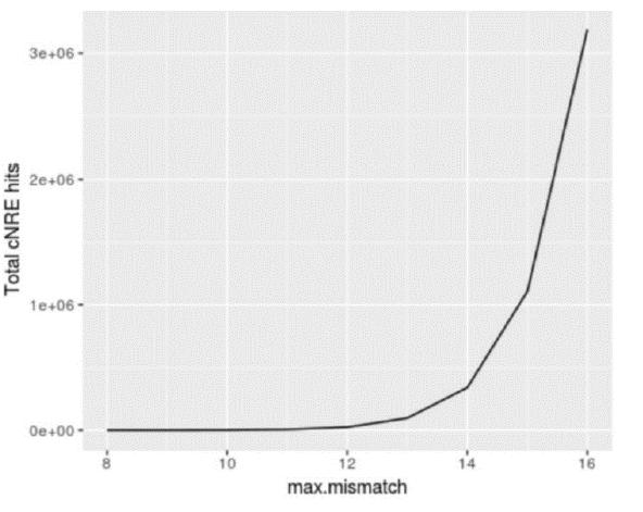
Figure 1: Number of cNRE hits to galGal5 according to maximum mismatches allowed: the cNRE is not an abundant low complexity sequence, but rather a rare repetitive sequence with a clear cutoff level of mismatches allowed. Consistent with this, there are only two (2) cNRE sequences in chromosome 19, the chromosome that contains the AMHC1 gene (the chicken ortholog of the quail SMyHC III gene). ## [1] chr19 [16510, 16541] * | 5’-CAAGGACAAAGAGGGGACAAAGAGGCGGAGGT-3 ## [2] chr19 [32821, 32852] * ‘5’-CAAGGACAAAGAGTGGACAAAGAGGCAGACGT-3
In the evolutionary strategy, which we now include, we first mapped the phylogenetic origins of the SMyHC III family of slow myosins and then established how and when the cNREs became topologically associated with the SMyHC III gene. To do that we repeat masked all available sequences from avian SMyHC III orthologs. As it will become clear below, the cNRE is a rare sequence, rather than a low complexity repeat. Our search for cNREs outside of the quail context (Coturnix coturnix) followed two independent lines. First, we took a scaled, evolution-oriented approach. Initially, we looked for cNREs in species close to the quail (i.e., Galliformes) and then progressively farther, to include derived (i.e., Passeriformes) and basal avians (i.e., Paleognaths) as well as external groups such as crocodilians. While pursuing this line of investigation, it became clear that the cNRE was a rare form of repetitive element, which showed a conserved topological relationship with the SMyHC III gene (i.e., cNREs flanked the SMyHC III genes at 5’ and 3’ regions). Using this topological relationship as a character, we determined when it appeared during avian evolution, and then set out to establish the likely origins of this rare repetitive motif. This search for the origins of the cNRE entailed comparisons to databases of repetitive genome elements, until the extreme telomeric nature of the SMyHC III gene became evident. This finding directed us to the fact that the hexad nature of the cNRE is reminiscent of the hexameric character of telomeric direct repeats. Because direct telomeric repeats are exactly featured in the genomes of avian DNA viruses that can infect the germline and integrate into the avian genome (Morissette & Flamand, 2010), we focused our search for the cNRE on the members of the subfamily Alphaherpesvirinae. In this search, we utilized the human herpes simplex virus 1 (HSV1) as a general model for herpes viruses and a set of four (4) members of the Alphaherpesvirinae family that specifically infect Galliformes (i.e., GaHV1, the virus responsible for avian infectious laryngotracheitis in chickens, GaHV2, the Marek’s disease virus, GaHV3, a non-pathogenic virus and MeHV1, the non-pathogenic Meleagrid herpesvirus 1 capable of infecting chicken and wild turkey) (Waidner et al., 2009). The search for cNREs in Alphaherpesvirinae was successful. We found six (6) cNRE hits in HSV1 and one (1) cNRE was detected in GaHV1, but none in MeHV1, GaHV2, and GaHV3.
Our evolution-directed approach thus led to the direct recognition that cNREs up to a cutoff mismatch value of 11 can be found in the genomes of a family of viruses that contain members that infect avians and integrate their double-stranded DNA into the host germline. Therefore, as a second independent approach, we set out to extend this proof of concept by broadening our search to all known sequenced viruses to perform an unbiased, internally consistent, and quantitative analysis of cNRE presence in viral genomes, as already reported in the initial submission of this manuscript.
Author Response:
Reviewer #1 (Public Review):
In this study, Kuppan, Mitrovich, and Vahey investigated the impact of antibody specificity and virus morphology on complement activation by human respiratory syncytial virus (RSV). By quantifying the deposition of components of the complement system on RSV particles using high-resolution fluorescence microscopy, they found that antibodies that bind towards the apex of the RSV F protein in either the pre- or post-fusion conformation activated complement most efficiently. Additionally, complement deposition was biased towards globular RSV particles, which were frequently enriched in F in the post-fusion conformation compared to filamentous particles on which F exists predominantly in the pre-fusion conformation.
Strengths:
1) While many previous studies have examined the properties of antibodies that impact Fc-mediated effector functions, this study offers a conceptual advance in its demonstration that heterogeneity in virus particle morphology impacts complement activation. This novel finding will motivate further research on this topic both in the context of RSV and other viral infections.
2) The use of site-specific labeling of viral proteins and high-resolution fluorescence microscopy represents a technical advance in monitoring interactions among different components of antiviral immune responses at the level of single virus particles.
3) The paper is well written, data are clearly presented and support key claims of the paper with caveats appropriately acknowledged.
We appreciate the reviewer’s supportive comments. In our revised manuscript, we have focused on improving clarity regarding the minor weaknesses noted below.
Minor weaknesses:
Working models and their implications could be clarified and extended. Specifically:
1) The finding that globular particles enriched in F proteins in the post-fusion conformation (Fig 3F) are dominant targets of complement activation as measured by C3 deposition by not only post-F- but also pre-F-specific antibodies (Fig 4B, left) is interesting. This is despite the fact that, as expected, pre-F antibodies bind less efficiently to globular particles (Fig 4B, right). How do the authors reconcile these observations, given that C3 deposition seems to be IgG-concentration-dependent (Fig 2E)?
The reviewer raises an excellent point: globular particles, which accumulate as the virus ages, contain more post-F and less pre-F than particles that have recently been shed from infected cells. These ‘aged’ particles nonetheless accumulate more C3 when incubated with pre-F mAbs than ‘younger’ particles, where the proportion of pre-F is higher. We attribute this to the lower surface curvature of globular particles: they accumulate more C3 in the presence of pre-F mAbs in spite of the reduced availability of pre-F epitopes. Figure 1C and 1F help to support this point. This data shows C3 deposition driven by different antibodies bound to particles enriched in either pre-F (Figure 1C) or post-F (Figure 1F). Importantly, for this experiment the conversion to post-F was driven in such a way that virion morphology is preserved (Figure 1E). In this case, we see a clear reduction in C3 deposition by pre-F mAbs on post-F particles (e.g. for CR9501, the percentage of C3-positive particles drops from 24% on pre-F virus to 6% on post-F-enriched virus). This demonstrates that, in the absence of other changes, conversion of pre-F to post-F reduces complement deposition by pre-F specific mAbs.
Similarly, the reviewer correctly points out that reduced levels of antibody binding lead to lower levels of C3 deposition (Figure 2E); however, as in Figure 1, this data is collected from particles with the same morphologies. Thus, in the absence of additional factors, reduction in mAbs bound to pre-F leads to a reduction in C3 deposition driven by these mAbs. The fact that we observe the opposite trend when changes in particle morphology accompany changes in post-F abundance points to an important role for particle shape in activation of the classical pathway.
2) Based on data in Figure 5-figure supplement 2, the authors argue that "large viruses are poised to evade complement activation when they emerge from cells as highly-curved filaments, but become substantially more susceptible as they age or their morphology is physically disrupted." Could the increase in C3 deposition be alternatively explained by a higher density of F proteins on larger particles instead of / in addition to a larger potential decrease in membrane curvature?
We agree that the density of F on a virus – the number of F trimers per unit surface area - likely contributes to the efficiency of C3 deposition. In Figure 6 – figure supplement 2 (Figure 5 – figure supplement 2 in the original submission), we control for this potential effect by comparing viruses that have the same amount of F (as measured by fluorescence intensities of SrtA-labeled F) that are either in filamentous form or globular form (induced through osmotic swelling). The total amount of F per virus is preserved during swelling, and the membrane surface area will remain constant due to the limited ability of lipid bilayers to stretch7. As a result, the input material for these comparisons is the same in terms of F trimers per unit area, yet the C3:F ratio differs substantially. This leads us to conclude that the differences must be attributable to factors other than the density of F. Importantly, this does not mean that the amount of F per unit surface area does not matter for C3 deposition – only that this is not the effect we are observing here. We have added text (Line 299) to help clarify this point: “This effect is unlikely to arise due to changes in the abundance or density of F in the viral membrane, both of which will remain constant following swelling. Similarly, it does not appear to be purely related to size, as larger viral filaments show similar C3:F ratios as smaller viral filaments.”
3) In the discussion, the authors acknowledge that the implications based on the findings are speculative. However, more clarity on the basis of these speculative models would be useful. For example, it is not clear how the findings directly inform the presented model of immunodominance hierarchies in infants.
We agree that this was unclear in the original manuscript. We have rewritten paragraph 4 of the Discussion to clarify how our results may contribute to the changes in immunodominance that have been observed in RSV between infants and adults.
Reviewer #2 (Public Review):
This is an intriguing study that investigates the role of virus particle morphology on the ability of the first few components in the complement pathway to bind and opsonize RSV virions. The authors use primarily fluorescence microscopy with fluorescently tagged F proteins and fluorescently labeled antibodies and complement proteins (C3 and C4). They observed that antibodies against different epitopes exhibited different abilities to induce C3 binding, with a trend reflecting positioning of IgG Fc more distal to the viral membrane resulting in better complement "activation". They also compared the ability of C3 to deposit on virus produced from cells +/- CD55, which inhibits opsonization, and showed knockout led to greater C3 binding, indicating a role for this complement "defense protein" in RSV opsonization. They also examined kinetics of complement protein deposition (probed by C4 binding) to globular vs filamentous particles, observing that deposition occurred more rapidly to non-filaments.
A better understanding of complement activation in response to viruses can lead to a more comprehensive understanding of the immune response to antigen both beneficial and detrimental, when dysfunctional, during infection as well as mechanisms of combating the viral infection. The study provides new mechanistic information for understanding the properties of an enveloped virus that can influence complement activation, at least in an in vitro setting. It remains to be determined whether these effects manifest in the considerably more complex setting of natural infection or even in the presence of a polyclonal antibody mixture.
The studies are elegantly designed and carefully executed with reasonable checks for reproducibility and controls, which is important especially in a relatively complex and heterogeneous experimental system.
We thank the reviewer for the insightful comments. We have revised the manuscript to help to clarify points of confusion and to address some of the technical points raised here.
Specific points:
1) "Complement activation" involves much more than C3 or C4 binding. Better to use more specific terminology relating to the observable (i.e. fluorescently labeled complement component binding)
We agree with the reviewer. We have revised the manuscript throughout to make our language more accurate and precise.
2) What is the rationalization for concentrations of antibodies used? What range was tested, and how dependent on antibody concentration were the observed complement deposition trends? How do they relate to physiological concentrations, and how would the presence of a more complex polyclonal response that is typically present (e.g. as the authors noted, the serum prior to antibody depletion already mediates complement activation) affect the complement activation trends? The neat, uniform display of Fc for monoclonals that were tested is likely to be quite garbled in more natural antibody response situations. This should be discussed.
We have added discussion of antibody concentrations and possible differences between monoclonal and polyclonal responses to the revised manuscript. Below, we address the specific questions raised here by the reviewer.
We chose to use antibody concentrations that are comparable to the concentrations of dominant clonotypes in post-vaccination serum1. Our goal in selecting relatively high antibody concentrations for our experiments was to focus on understanding the capacity of an antibody to drive complement deposition when it has reached maximum densities on RSV particles. This is discussed starting on Line 125 of Results, and in paragraph 2 of Discussion. Experiments testing a range of antibody concentrations would be valuable, but are likely to strongly reflect differences in the binding affinities of these antibodies, which have been characterized previously.
Although we have not performed titrations for each of the antibodies tested due to the large number of conditions needed and the limited throughput of our experimental approach, the manuscript does present a dilution series for CR9501, the IgG1 mAb with the greatest potency in driving C3 deposition among those tested here. This data (shown in Figure 3E & F in the revised manuscript) shows that as the amount of antibody added in solution decreases over a 16-fold range, C3 deposition decreases as well. The decrease in C3 deposition is roughly commensurate with the reduction in antibody binding, reaching levels that are just above background at an antibody concentration of ~0.6μg/ml (1:800 dilution). We think it is likely that other activating antibodies would show similar trends, while antibodies that do not activate the classical pathway at saturating concentrations would be unlikely to do so across a range of lower concentrations.
We agree with the reviewer that complement deposition driven by polyclonal antibodies is more complex than the monoclonal responses studied here. As discussed in paragraph 2 of our revised Discussion, one effect that polyclonal serum might have is to increase the density of Fcs on the virus by providing antibody mixtures that bind to multiple non-overlapping antigenic sites. We speculate that this would generally increase complement deposition, provided that sufficient antibodies are present that bind to productive antigenic sites (e.g. sites 0/ , II, and V).
Finally, we note that we observe a similar phenomenon where globular particles are preferentially opsonized with C3 in our experiments with polyclonal serum where IgG and IgM have not been depleted (Figure R1). The major limitation of this data – which is resolved by using monoclonal antibodies – is the difficulty of determining to what extent this bias arises due to the epitopes targeted by the polyclonal serum versus the intrinsic sensitivity of the virus particles.
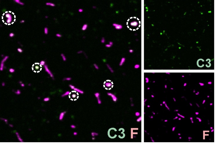
Figure R1: RSV opsonized with polyclonal human serum. A similar bias towards globular particles (white dashed circles) is observed as in experiments with monoclonal antibodies.
3) Are there artifacts or caveats resulting from immobilization of virus particles on the coverslips?
As pointed out by the reviewer, a few possible artifacts or caveats could arise due to the immobilization of viruses on coverslips. These include (1) spurious binding of C1 or other complement components to the immobilizing antibody (3D3); (2) reduced access to viral antigens as a result of immobilization; and (3) inhibition of antibody-induced viral aggregation. We are able to rule out issues associated with (1), because we do not see attachment of C1 or C3 to the coverslip (i.e. outside regions occupied by virus particles). This is consistent with the fact that the antibodies are immobilized on the surface via a C-terminal biotin attached to the heavy chain, which would limit access for C1 binding and prevent the formation of Fc hexamers.
Immobilization on coverslips could reduce the accessibility of a portion of the virus for binding by antibodies and complement proteins. This could effectively shield a portion of the viral surface from assembly of an activating complex, which we estimate requires ~35nm of clearance above the targeted epitope on F8. Importantly, the fraction of the viral surface area that would be shielded would vary for filaments and spheres; to determine if this could influence our results, we calculated the expected magnitude of this effect (Figure R2). To do this, we modeled the virus as being tethered to the surface via a 25nm linkage. This accounts for the length of the biotinylated PEG (~5-15nm for PEG2K, depending on the degree of extension), streptavidin (~5nm), and the anti-G antibody (~10-15nm including the biotinylated C-terminal linker). Although limited structural information is available for RSV G, the ~100 residue, heavily glycosylated region between the viral membrane and the 3D3 epitope likely extends above the height of F (~12nm). Our model assumes that a shell of thickness d surrounding the virus is necessary for antibody-C1 complexes to fit without clashing with the surface (this shell is shaded in gray in the schematic from Figure R2). Tracing the angles at which this shell clashes with the coverslip allows us to calculate the fraction of total surface area that is inaccessible for activation of the classical pathway. The results are plotted on the right side of Figure R2. The relative surface area accessible to a 35nm activating antibody-C1 complex differs between a filament and a sphere of equivalent surface area by about 15%. We conclude that this difference is modest compared to the ~5-fold difference in deposition kinetics we observe between viral filaments and spheres (Figure 4), or the 3- to 10-fold difference in relative C3 deposition we observe on larger filamentous particles after conversion to spheres (Figure 6 – figure supplement 2C).
Finally, by performing experiments on immobilized viruses, we eliminate the possibility for antibody-dependent particle aggregation. While this was necessary for us to get interpretable results, the formation of viral aggregates could affect the dynamics and extent of complement deposition. For example, activation of the classical pathway on one particle in an aggregate could spread to non-activating particles through a “bystander effect”, as has been reported in other contexts9. We are interested in this question and have begun preliminary experiments in this direction; however, we believe that a definitive answer is outside the scope of this current work. To alert readers to this consideration, we have added this to paragraph 2 of the revised Discussion (Line 359).
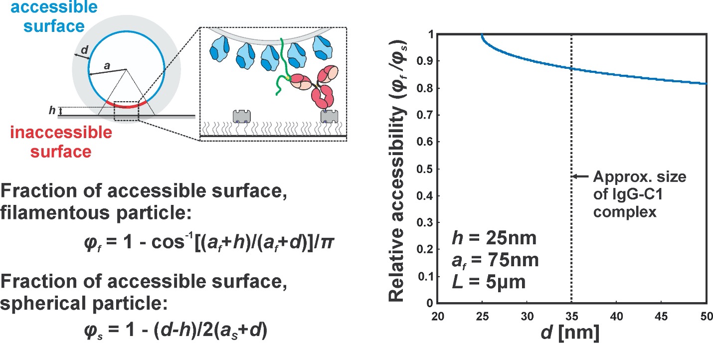
Figure R2: Estimating the surface accessibility of RSV particles bound to coverslips. Definition of variables: af: radius of cylindrical RSV filament; as: radius of spherical RSV particle of equivalent surface area (see Figure 6 – figure supplement 2A); d: distance needed above the viral surface to accommodate IgG-C1 activating complexes; h: height of viral surface above the coverslip; L: length of the viral filament.
4) How is the "density of antigen" quantitated? What fraction of F or G is labeled? For fluorescence intensity measurements in general, how did the authors ensure their detection was in a linear sensitivity range for the detectors for the various fluorescent channels? Since quantitation of fluorescence intensities is important in this study, some discussion in methods would be valuable.
We have performed this important additional characterization of our fluorescence system and our overall labeling and quantification strategy to address these concerns. The results of this characterization are now included in two new figure supplements in the revised manuscript (Figure 1 – figure supplements 2 & 3).
5) The authors also show that the particle morphology, whether globular or filamentous, as well as relative size and resulting apparent curvature, correlate with ability of C3 to bind. Some link to the abundance of post-fusion F (post-F) is examined and discussed, but I found the back and forth discussion between morphology, C3 binding, and post-F abundance to be confusing and in need of clarification and streamlining. Is there a mechanistic link between morphology changes and post-F level increases? Are the two linked or coincidental (for example does pre-F interaction with matrix help stabilize that conformation, and if lost lead to spontaneous conversion to post-F?). Please clarify.
Specifically, we have separated the discussion of pre-F versus post-F abundance and particle morphology into two different sections in Results, and we have rearranged Figures 4 and 5 (Figures 3 and 4 in the original submission) to improve clarity.
Regarding the question of whether changes in morphology and the pre-F to post-F conversion are coincidental or mechanistically linked: the answer is not entirely clear, although we have collected new data that suggests a connection. We first want to note that the two effects are at least partly separable: brief treatment with a low osmolarity solution causes particle shape to change while preserving pre-F (Figure 6A & B), whereas treating with an osmotically balanced solution with low ionic strength converts pre-F to post-F without affecting virus shape (Figure 1E). However, we were motivated by the reviewer’s questions to look into this further. To determine if the change in viral shape may serve to destabilize the pre-F conformation over time, we compared the relative amounts of pre-F and post-F present in particles that were osmotically swollen to those that were not at 0h and at 24h. In these experiments, particles were swollen using a brief (~1 minute) exposure to low osmolarity conditions before returning them to PBS (Figure R3, left). As expected, we observe no immediate change in pre-F abundance following the brief osmotic shock (Figure R3, right: 0h time point), consistent with Figure 6B. After incubating the particles an additional 24h at 37oC, the post-F-to-pre-F ratio is ~3.5-fold higher in osmotically-swollen particles than in those where filamentous morphology was initially preserved (Figure R3, right: 24h time point). This supports the reviewer’s suggestion that interactions with the matrix may help to stabilize F in the prefusion conformation, since the conversion to post-F is faster when this interaction is disrupted. Whether or not this has any relevance for RSV entry into cells remains to be determined; however, it is worth noting that we observed no clear loss or gain of infectivity in RSV particles following osmotic swelling (Figure 6 – figure supplement 1A). Since this result may be of interest to readers, we have included this new data in Figure 6 – figure supplement 1B, and it is discussed briefly in Results (Line 250).
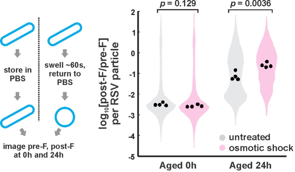
Figure R3: Determining stability of pre-F following matrix detachment. Left: Experimental design. Right: Comparison of pre-F stability on untreated particles (gray) and particles subjected to brief osmotic swelling (magenta). Distributions show the ratio of post-F (ADI-14353) to pre-F (5C4) intensities per particle, combined for four biological replicates, sampled at 0h (immediately after swelling) and after an additional incubation at 37oC for 24h. Black points show median values for each individual replicate. P-values are determined from a two-sample T test.
6) Since their conclusion is that curvature of the virus surface is a major influence on the ability of complement proteins to bind, I feel that some effort at modeling this effect based upon known structures is warranted. One might also anticipate then that there would be some epitope-dependent effect as a result of changes in curvature that may lead to an exaggeration of the epitope-specific effects for more highly curved particles perhaps than those with lower curvature? Is this true?
The reviewer raises two excellent points: that it may be possible to gain insight into the mechanisms through which curvature dictates C1 binding and other aspects of complement activation through structural modeling, and that such a model may help to identify specific epitope effects that could contribute to curvature dependence.
We developed simulations based on the geometry of RSV, F, and hexameric IgG to try to better understand how curvature may influence initiation of the classical pathway. This model is described in the Methods section (Modeling IgG hexamers on curved surfaces), and the results are discussed in the final two paragraphs of the Results section. In addition, we have included a new figure (Figure 7) to summarize the model’s predictions. This model corroborates the curvature sensitivity of IgG hexamer formation and suggests a possible intuitive explanation for our findings: high curvature effectively increases the distance between epitopes that sit high above the viral membrane, decreasing the likelihood of hexamer formation (Figure 7D). Regarding epitope specific effects, this model suggests that the further the epitope is above the viral membrane, the greater the effect that decreasing curvature will have. However, we find that epitopes closer to the membrane (e.g. those bound by 101F or ADI-19425) are overall very inefficient at activating the classical pathway, potentially due to steric obstruction of the formation of IgG hexamers. Thus, there may be an inherent tradeoff between overcoming steric obstruction (by binding to epitopes distal to the membrane) and sensitivity to surface curvature.
It is important to note that this model is reductionist and does not include detailed structural information. Additional factors may be important for considering epitope-specific effects. For example, antibodies that bind equatorially on F (e.g. ADI-19425, which binds to antigenic site III), show minimal complement deposition in our experiments. However, particles whose curvature approaches the diameter of hexameric IgG or IgM (~20nm) may display these epitopes in a manner that is more accessible. If the curvature necessary to observe such an effect falls outside of the biologically accessible range, it would not be observable in our experiments. Nonetheless, it is possible that a different set of antibodies may drive complement deposition on highly-curved nanoparticle vaccines that are in development10. We have added this important point to the second paragraph of the Discussion.
7) Line 265: it would be useful to confirm the increase C1 binding as a function of morphology as was done for antibody-angle of binding experiments.
We believe that this data is shown in Figure 6B (Figure 5B in the original manuscript).
Reviewer #3 (Public Review):
Overall the manuscript is clearly written and the data are displayed well, with helpful diagrams in the figures to illustrate assays and RSV F epitopes. The engineering of the RSV strain to include a fluorescent reporter and tags on F and G that serve as substrates for fluorophore attachment is impressive and is a strength. The RSV literature is well cited and the interpretation of the results is consistent with structure/function data on RSV F and its interaction with antibodies. This reviewer is not an expert on the experiments performed in this manuscript, but they appear to be rigorously performed with appropriate controls. As such, the conclusions are justified by the data. One weakness is the extent to which the results regarding virion morphology are biologically relevant. Non-filamentous forms of the virion are generally obtained only in vitro as a result of virion purification or biochemical treatment. However, these results may be relevant for certain vaccine candidates, including the failed formalin-inactivated RSV vaccine that was evaluated in the late 1960s and caused vaccine-enhanced disease upon natural RSV infection.
Thank you for these suggestions, which have helped us to better place our results regarding RSV morphology in the context of prior work. We agree with the reviewer that non-filamentous RSV particles are commonly obtained in vitro, and that this morphology does not reflect the structure of the virus as it is budding from infected cells. Our work has characterized the transition from filament to globular / amorphous form, with the finding that it can occur rapidly upon physical or chemical perturbations, as well as more gradually during natural aging: i.e. in the absence of handling or purification. We are also able to detect globular particles accumulating in cultured A549 cells, where no handling has occurred prior to observation (Figure 5 – figure supplement 1). While we do not currently know how well this reflects the tendency of RSV to undergo conversion from filament to sphere in vivo, we propose that it is plausible that such a transformation could occur. To distinguish between what we demonstrate and what we speculate, we write (Line 401): “Although more work is needed to understand the prevalence of globular particles during in vivo infection, our observations that these particles accumulate over time through the conversion of viral filaments – even under normal cell culture conditions - suggest that their presence in vivo is feasible, where the physical and chemical environment would be considerably harsher and more complex.”
We agree with the reviewer that our results may have relevance towards understanding the failed formalin-inactivated vaccine trial. We have added this to paragraph 5 of the Discussion section.
Author Response:
Reviewer #2 (Public Review):
- The novelty of the current observation of two types of links is overstated, for example, in the abstract: "Our data reveal the existence of two molecular connectors/spacers which likely contribute to the nanometer scale precise stacking of the ROS disks" (Line 25). In fact, both of these links have been shown before (Usukura and Yamada, 1981; Roof and Heuser, 1982; Corless and Schneider, 1987; Corless et al., 1987; Kajimura et al., 2000). These previous studies deserve to be recognized. Of special note is the paper by Usukura and Yamada whose images of the disc rim connectors are by no means less convincing than shown in the current manuscript. On the other hand, the novelty and impact of the data related to peripherin appears to be understated, particularly in the abstract.
We changed the abstract line 27 to: “Our data confirm the existence of two previously observed molecular connectors …”, cite the recommended references in the introduction (lines 54-55), the results (lines 131-132), and the discussion (lines 282/285). To highlight the previous reports, we rephrased the sentence in lines 132-133, “In agreement with these previous findings, we observed structures that connect membranes of two adjacent disks …”; the discussion is rephrased in lines 280-281, “Similar connectors have been observed previously ...” and “… and their statistical analysis confirmed the existence of two distinct connector species.”, and in lines 291-292, “Based on previous studies combined with our quantitative analysis, we put forward a hypothesis for the molecular identity of the disk rim connector which agrees in part with recent models”.
- Notably, ROM-1 has not been found in peripherin oligomers larger than octamers (e.g. Loewen and Molday, 2000 and subsequent studies by Naash and colleagues). This should be discussed in the context of the current model.
We agree that this is an important aspect. We pick subvolumes along all disk rims, and on average we obtain the ordered scaffold as shown in the manuscript. We expect heterogeneity in the data because of the different degrees of oligomerization and the exclusion of ROM1 from higher oligomers. Our analysis required substantial classification to achieve convergence to a stable average, indeed indicating heterogeneity in the rim structure. However, we could not resolve additional structures to sufficient quality. It might be that this heterogeneity is what ultimately limits our achievable resolution. We added these thoughts in the discussion starting in lines 377-378, “PRPH2-Rom1 oligomers isolated from native sources exhibit varying degrees of polymerization (Loewen and Molday, 2000), and ROM1 is excluded from larger oligomers (Milstein et al., 2020). We could not resolve this heterogeneity as additional structures to sufficient quality by subvolume averaging, but in combination with the inherent flexibility of the disk rim, this heterogeneity might be the reason for the restricted resolution of our averages.”
- The following statement should be reconsidered given the established role of cysteine-150 in peripherin oligomerization: "We hypothesize that the necessary cysteine residues are located in the head domain of the tetramers (Figure 5B), ..." It has been firmly established that only one cysteine (C150) located in the intradiscal loop is not engaged in intramolecular interactions and is essential for peripherin oligomerization.
Thank you for this advice. We agree and rephrased our discussion in lines 368-371, “The intermolecular disulfide brides are exclusively formed by the PRPH2-C150 and ROM1-C153 cysteine residues, which are located in the luminal domain (Zulliger et al., 2018). We hypothesize that these disulfide bonds (Figure 5B), are responsible for the contacts across rows (Figure 3) ...”
- Line 340: "A model involving V-shaped tetramers for membrane curvature formation was proposed recently (Milstein et al., 2020), but it comprises two rows of tetramers which are linked in a head-tohead manner. Our analysis instead resolves three rows organized side-by side in situ (Figure 5A)." I am confused by this statement: doesn't your model also show long rows connected head-to-head? The real difference is that Milstein and colleagues proposed four tetramers per rim whereas the current data reveal three.
Thank you for pointing out this imprecise description. The model proposed by Milstein and the model in the old version of our manuscript, both propose linkage between tetramers via their disk luminal domains. In our manuscript, we refer to the luminal domain as the head domain. However, to our understanding, the Milstein model suggests two rows of tetramers, where one tetramer in the first row is rotated 180° with respect to a tetramer in the second row (therefore head-to-head), while our data indicate that the V-shaped repeats which we originally hypothesized to be tetramers are only rotated ~63° with respect to one another and are therefore rather oriented side-by-side:
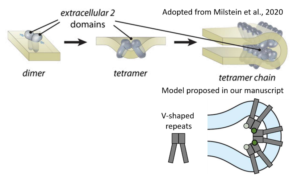
Fig. 2: Comparison of models for the organization of the ROS disk rim as proposed in in Milstein et al., 2020 (top panel)
and in our work (lower panel). We now rephrased lines 383-385, “Instead, our analysis in situ resolves three rows of repeats which are also linked by the luminal domain but are rather organized side-by-side (Figure 5A).”
- Line 347: "Our data indicate that the luminal domains of tetramers hold the disk rim scaffold together (Figure 3C), which is supported by the fact that most pathological mutations of PRPH2 affect its luminal domain (Boon et al., 2008; Goldberg et al., 2001). It is possible that these mutations impair the formation of tetramers, rows of tetramers, and their disulfide bond-stabilized oligomerization. These alterations could impede or completely prevent disk morphogenesis which, in turn, would disrupt the structural integrity of ROS, compromise the viability of the retina and ultimately lead to blindness." This is not an original idea, as many studies showed that disruptions in peripherin oligomerization lead to anatomical defects in disc formation and subsequent photoreceptor cell death.
Thank you for pointing this out. Our data are indeed in good agreement with the results made by many groups and further expand on them. We rephrased the manuscript in several places to clarify this relationship: in the abstract lines 32-34, “Our Cryo-ET data provide novel quantitative and structural information on the molecular architecture in ROS and substantiate previous results on proposed mechanisms underlying pathologies of certain PRPH2 mutations leading to blindness.”; in the introduction lines 78-79, “… allowed us to obtain 3D molecular-resolution images of vitrified ROS in a close-to-native state providing further evidence for previously suggested mechanisms leading to ROS dysfunction”; and in the discussion lines 393-397, “In good agreement with previous work, it is possible that these mutations impair the formation of complexes, and their disulfide bond-stabilized oligomerization (Chang et al., 2002; Conley et al., 2019; Zulliger et al., 2018). Hence, these alterations could impede or completely prevent disk morphogenesis …”. Also, additional relevant publications are cited in line 395.
- In regards to the distance between disc rims and plasma membrane, the authors cite the data obtained with frogs (10 nm) but not a more relevant, previously reported measurement in mice (Gilliam et al, 2012). The value of 18 nm reported in that study is much closer to the currently reported value.
We appreciate the reference to this excellent paper. We added it in lines 335-337, “This value was derived from amphibians (Roof and Heuser, 1982) and deviates considerably from recent results (18 nm, (Gilliam et al., 2012)) and from our current measurements in mice (~25 nm).” Our aim was to point out that a model for ROS organization that is often cited and is otherwise well-founded (BatraSafferling et al., 2006) makes a wrong assumption about distance in the context of the mammalian systems. 7. The authors are (correctly) being very careful in assigning the molecular identity of disc interior connectors to PDE6. However, they are more confident in assigning the disc rim connectors to GARP2, which is reflected in the labeling of these links in figure
- Their arguments are valid, but these links are not attached to peripherin (a protein considered to be the membrane binding partner for GARPs), which is not immediately consistent with this hypothesis. Perhaps it would be fair to re-label the corresponding links in figure 5 as "disc rim connectors".
That is an excellent and fair suggestion. We changed Figure 5 accordingly.
- On a similar note, the disc rim connectors seem to be located where ABCA4 is presumed to be localized within the rim, which may not be just a coincidence. The authors already have tomograms obtained from ABCA4 knockout animals. Is it possible to analyze whether these links are preserved in these tomograms?
We agree, this is an important question to address. Unfortunately, neither the biological preparation nor the tomograms of the ABCA4 knockout were as good in quality as for the WT. Still, we frequently see connectors at the disk rim, especially after denoising of the tomograms.
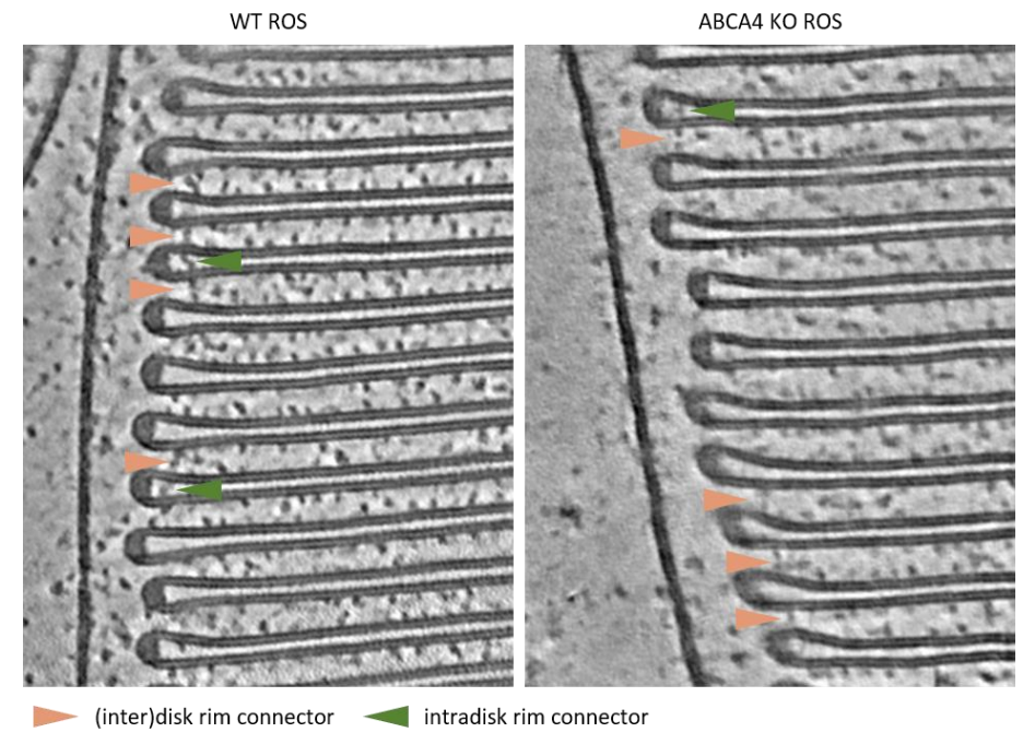
Fig. 3: connectors at disk rims in WT (left) and ABCA4 knockout mice (right).
Sometimes it appears the connectors between adjacent disks are linked via an intradisk densities, which was already observed in Corless et al., 1987. We thought that these densities could be ABCA4 and tried to find them with two approaches in our WT tomograms (data not shown). In the first approach using a segmentation similar to what we did for the connectors between disks, we found an order of magnitude fewer intradisk connectors than (inter)disk rim connectors. In the second approach, we used the positions of segmented (inter)disk rim connectors and classified rotational averages which focused on the disk luminal space next to the contact point of a connector with the disk membrane. Again, less than 10% of the disk rim connector subvolumes were assigned to classes with an additional luminal density. Both experiments indicate that disk rim connectors sometimes occur with an additional luminal density. In total, we found less than 100 of these intradisk densities, an observation which seems to be preserved in WT and ABCA4 KO. Based on this small number of positions/locations, however, we cannot draw any conclusion. Therefore, we did not add this point to the manuscript.
Author Response
Public Evaluation Summary:
The authors re-analyzed a previously published dataset and identify patterns suggestive of increased bacterial biodiversity in the gut may creating new niches that lead to gene loss in a focal species and promote generation of more diversity. Two limitations are (i) that sequencing depth may not be sufficient to analyze strain-level diversity and (ii) that the evidence is exclusively based on correlations, and the observed patterns could also be explained by other eco-evolutionary processes. The claims should be supported by a more detailed analysis, and alternative hypotheses that the results do not fully exclude should be discussed. Understanding drivers of diversity in natural microbial communities is an important question that is of central interest to biomedically oriented microbiome scientists, microbial ecologists and evolutionary biologists.
We agree that understanding the drivers of diversity in natural communities is an important and challenging question to address. We believe that our analysis of metagenomes from the gut microbiomes is complementary to controlled laboratory experiments and modeling studies. While these other studies are better able to establish causal relationships, we rely on correlations – a caveat which we make clear, and offer different mechanistic explanations for the patterns we observe.
We also mention the caveat that we are only able to measure sub-species genetic diversity in relatively abundant species with high sequencing depth in metagenomes. These relatively abundant species include dozens of species in two metagenomic datasets, and we see no reason why they would not generalize to other members of the microbiome. Nonetheless, further work will be required to extend our results to rarer species.
Our revised manuscript includes two major new analyses. First, we extend the analysis of within-species nucleotide diversity to non-synonymous sites, with generally similar results. This suggests that evolutionarily older, less selectively constrained synonymous mutations and more recent non-synonymous mutations that affect protein structure both track similarly with measures of community diversity – with some subtle differences described in the manuscript.
Second, we extend our analysis of dense time series data from one individual stool donor and one deeply covered species (B. vulgatus) to four donors and 15 species. This allowed us to reinforce the pattern of gene loss in more diverse communities with greater statistical support. Our correlational results are broadly consistent with the predictions of DBD from modeling and experimental studies, and they open up new lines of inquiry for microbiome scientists, ecologists, and evolutionary biologists.
Reviewer #1 (Public Review):
This paper makes an important contribution to the current debate on whether the diversity of a microbial community has a positive or negative effect on its own diversity at a later time point. In my view, the main contribution is linking the diversity-begets-diversity patterns, already observed by the same authors and others, to genomic signatures of gene loss that would be expected from the Black Queen Hypothesis, establishing an eco-evolutionary link. In addition, they test this hypothesis at a more fine-grained scale (strain-level variation and SNP) and do so in human microbiome data, which adds relevance from the biomedical standpoint. The paper is a well-written and rigorous analysis using state-of-the-art methods, and the results suggest multiple new experiments and testable hypotheses (see below), which is a very valuable contribution.
We thank the reviewer for their generous comments.
That being said, I do have some concerns that I believe should be addressed. First of all, I am wondering whether gene loss could also occur because of environmental selection that is independent of other organisms or the diversity of the community. An alternative hypothesis to the Black Queen is that there might have been a migration of new species from outside and then loss of genes could have occurred because of the nature of the abiotic environment in the new host, without relationship to the community diversity. Telling the difference between these two hypotheses is hard and would require extensive additional experiments, which I don't think is necessary. But I do think the authors should acknowledge and discuss this alternative possibility and adjust the wording of their claims accordingly.
We concur with the reviewer that the drivers of the correlation between community diversity and gene loss are unclear. Therefore, we have now added the following text to the Discussion:
“Here we report that genome reduction in the gut is higher in more diverse gut communities. This could be due to de novo gene loss, preferential establishment of migrant strains encoding fewer genes, or a combination of the two. The mechanisms underlying this correlation remain unclear and could be due to biotic interactions – including metabolic cross-feeding as posited by some models (Estrela et al., 2022; San Roman and Wagner, 2021, 2018) but not others (Good and Rosenfeld, 2022) – or due to unknown abiotic drivers of both community diversity and gene loss.”
Additionally, we have revised Figure 1 to show that strain invasions/replacements, in addition to evolutionary change, could be an important driver of changes in intra-species diversity in the microbiome.
Another issue is that gene loss is happening in some of the most abundant species in the gut. Under Black Queen though, we would expect these species to be most likely "donors" in cross-feeding interactions. Authors should also discuss the implications, limitations, and possible alternative hypotheses of this result, which I think also stimulates future work and experiments.
We thank the reviewer for raising this point. It is unclear to us whether the more abundant species would be donors in cross-feeding interactions. If we understand correctly, the reviewer is suggesting that more abundant donors will contribute more total biomass of shared metabolites to the community. This idea makes sense under the assumption that the abundant species are involved in cross-feeding interactions in the first place, which may or may not be the case. As our work heavily relies on a dataset that we previously analyzed (HMP), we wish to cite Figure S20 in Garud, Good et al. 2019 PLoS Biology in which we found there are comparable rates of gene changes across the ~30 most abundant species analyzed in the HMP. This suggests that among the most abundant species analyzed, there is no relationship between their abundance and gene change rate.
That being said, we acknowledge that our study is limited to the relatively abundant focal species and state now in the Discussion: “Deeper or more targeted sequencing may permit us to determine whether the same patterns hold for rarer members of the microbiome.”
Regarding Figure 5B, there is a couple of questions I believe the authors should clarify. First, How is it possible that many species have close to 0 pathways? Second, besides the overall negative correlation, the data shows some very conspicuous regularities, e.g. many different "lines" of points with identical linear negative slope but different intercept. My guess is that this is due to some constraints in the pathway detection methods, but I struggle to understand it. I think the authors should discuss these patterns more in detail.
We sincerely thank the reviewer for raising this issue, as it prompted us to investigate more deeply the patterns observed at the pathway level. In short, we decided to remove this analysis from the paper because of a number of bioinformatics issues that we realized were contributing to the signal. However, in support of BQH-like mechanisms at play, we do find evidence for gene loss in more diverse communities across multiple species in both the HMP and Poyet datasets. Below we detail our investigation into Figure 5b and how we arrived at the conclusion that is should be removed:
(1) Regarding data points in Figure 5B where many focal species have “zero pathways”,we firstly clarify how we compute pathway presence and richness. Pathway abundance data per species were downloaded from the HMP1-2 database, and these pathway abundances were computed using HUMAnN (HMP Unified Metabolic Analysis Network). According to HUMAnN documentation, pathway abundance is proportional to the number of complete copies of the pathway in the community; this means that if at least one component reaction in a certain pathway is missing coverage (for a sample-species pair), the pathway abundance may be zero (note that HUMAnN also employs “gap filling” to allow no more than one required reaction to have zero abundance). As such, it is likely that insufficient coverage, especially for low-abundance species, causes many pathways to report zero abundance in many species in many samples. Indeed, 556 of the 649 species considered had zero “present” pathways (i.e. having nonzero abundance) in at least 400 of the 469 samples (see figure below).
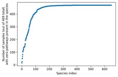
(2) We thank the reviewer for pointing out the “conspicuous regularities” in Figure 5B,particularly “parallel lines” of data points that we discovered are an artifact of the flawed way in which we computed “community pathway richness [excluding the focal species].” Each diagonal line of points corresponds to different species in the same sample, and because community pathway richness is computed as the total number of pathways [across all species in the sample] minus the number of pathways in the focal species, the current Figure 5B is really plotting y against X-y for each sample (where X is a sample’s total community pathway richness, and y is the pathway richness of an individual species in that sample). This computation fails to account for the possibility that a pathway in an excluded focal species will still be present in the community due to redundancy, and indeed BQH tests for whether this redundancy is kept low in diverse communities due to mechanisms such as gene loss.
We attempted to instead plot community pathway richness defined as the number of unique pathways covered by all species other than the focal species. This is equivalent to [number of unique pathways across all species in a sample] minus the [number of pathways that are ONLY present in the focal species and not any other species in the sample]. However, when we recomputed community pathway richness this way, it is rare that a pathway is present in only one species in a sample. Moreover, we find that with the exception of E. coli, focal species pathway richness tended to be very similar across the 469 samples, often reaching an upper limit of focal species pathway richness observed. (It is unclear to what extent lower pathway richnesses are due to low species abundance/low sample coverage versus gene loss). This new plot reveals even more regularities and is difficult to interpret with respect to BQH. (Note that points are colored by species; the cluster of black dots with outlying high focal pathway richness corresponds to the “unclassified” stratum which can be considered a group of many different species.)
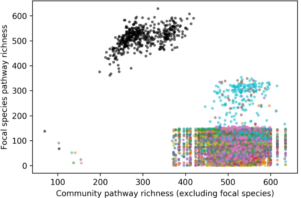
Overall, because community pathway richness (excluding a focal species) seems to primarily vary with sample rather than focal species in this dataset when using the most simple/strict definition of community pathway richness as described above, it is difficult to probe the Black Queen Hypothesis using a plot like Figure 5B. As pointed out by reviewers, lack of sequencing depth to analyze strain-level diversity and accurately quantify pathway abundance, irrespective of species abundance, seems to be a major barrier to this analysis. As such, we have decided to remove Figure 5B from the paper and rewrite some of our conclusions accordingly.
Finally, I also have some conceptual concerns regarding the genomic analysis. Namely, genes can be used for biosynthesis of e.g. building blocks, but also for consumption of nutrients. Under the Black Queen Hypothesis, we would expect the adaptive loss of biosynthetic genes, as those nutrients become provided by the community. However, for catabolic genes or pathways, I would expect the opposite pattern, i.e. the gain of catabolic genes that would allow taking advantage of a more rich environment resulting from a more diverse community (or at least, the absence of pathway loss). These two opposing forces for catabolic and biosynthetic genes/pathways might obscure the trends if all genes are pooled together for the analysis. I believe this can be easily checked with the data the authors already have, and could allow the authors to discuss more in detail the functional implications of the trends they see and possibly even make a stronger case for their claims.
We thank the reviewer for their suggestion. As explained above, we have removed the pathway analysis from the paper due to technical reasons. However, we did investigate catabolic and biosynthetic pathways separately as suggested by the reviewer as we describe below:
We obtained subsets of biosynthetic pathways and catabolic pathways by searching for keywords (such as “degradation” for catabolic) in the MetaCyc pathway database. After excluding the “unclassified” species stratum, we observe a total of 279 biosynthetic and 167 catabolic pathways present in the HMP1-2 pathway abundance dataset. Using the corrected definition of community pathway richness excluding a focal species, for each pathway type—either biosynthetic or catabolic—we plotted focal species pathway richness against community pathway richness including all pathways regardless of type:
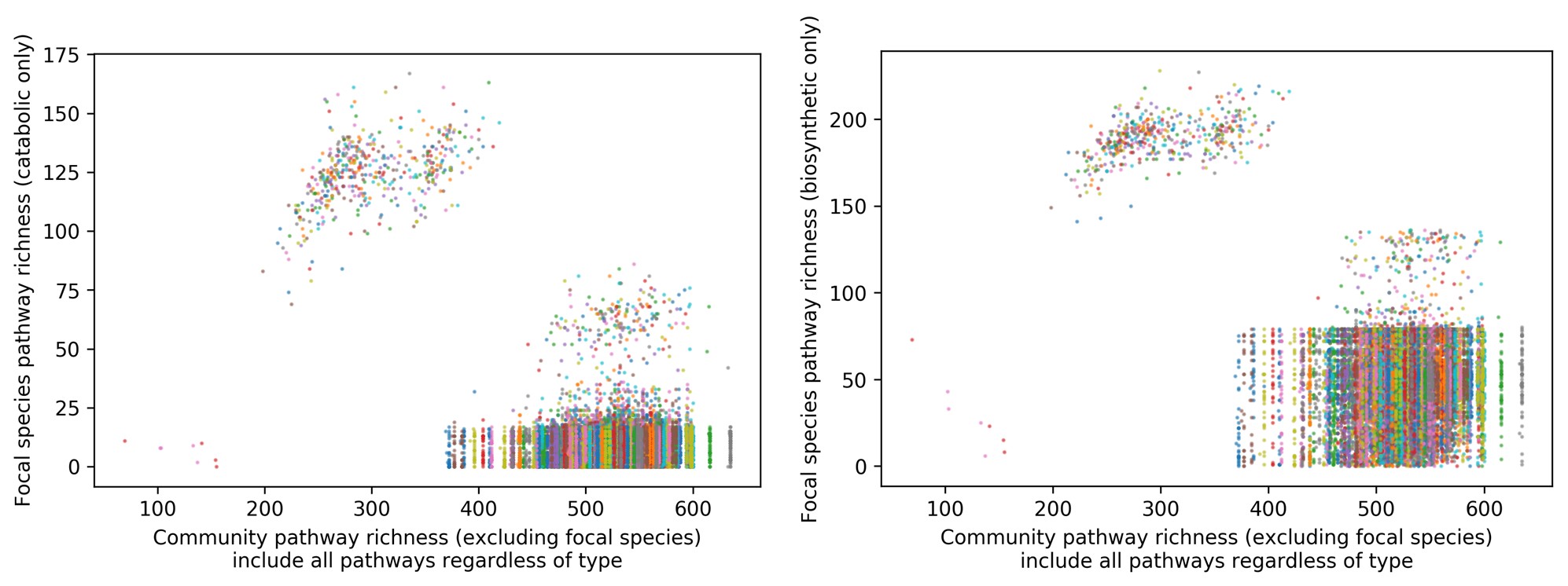
We observe the same problem where, within a sample, community pathway richness excluding the focal species hardly varies no matter which focal species it is, due to nearly all of its detected pathways being present in at least one other species; this makes the plots difficult to interpret.
Reviewer #2 (Public Review):
The authors re-analysed two previously published metagenomic datasets to test how diversity at the community level is associated with diversity at the strain level in the human gut microbiota. The overall idea was to test if the observed patterns would be in agreement with the "diversity begets diversity" (DBD) model, which states that more diversity creates more niches and thereby promotes further increase of diversity (here measured at the strain-level). The authors have previously shown evidence for DBD in microbiomes using a similar approach but focusing on 16S rRNA level diversity (which does not provide strain-level insights) and on microbiomes from diverse environments.
One of the datasets analysed here is a subset of a cross-sectional cohort from the Human Microbiome Project. The other dataset comes from a single individual sampled longitudinally over 18 months. This second dataset allowed the authors to not only assess the links between different levels of diversity at single timepoints, but test if high diversity at a given timepoint is associated with increased strain-level diversity at future timepoints.
Understanding eco-evolutionary dynamics of diversity in natural microbial communities is an important question that remains challenging to address. The paper is well-written and the detailed description of the methodological approaches and statistical analyses is exemplary. Most of the analyses carried out in this study seem to be technically sound.
We thank the reviewer for their kind words, comments, and suggestions.
The major limitation of this study comes with the fact that only correlations are presented, some of which are rather weak, contrast each other, or are based on a small number of data points. In addition, finding that diversity at a given taxonomic rank is associated with diversity within a given taxon is a pattern that can be explained by many different underlying processes, e.g. species-area relationships, nutrient (diet) diversity, stressor diversity, immigration rate, and niche creation by other microbes (i.e. DBD). Without experiments, it remains vague if DBD is the underlying process that acts in these communities based on the observed patterns.
We thank the reviewer for their comments. First, regarding the issue of this being a correlative study, we now more clearly acknowledge that mechanistic studies (perhaps in experimental settings) are required to fully elucidate DBD and BQH dynamics. However, we note that our correlational study from natural communities is complementary to experimental and modeling studies, to test the extent to which their predictions hold in more complex, realistic settings. This is now mentioned throughout the manuscript, most explicitly at the end of the Introduction:
“Although such analyses of natural diversity cannot fully control for unmeasured confounding environmental factors, they are an important complement to controlled experimental and theoretical studies which lack real-world complexity.”
Second, to increase the number of data points analyzed in the Poyet study, we now include 15 species and four different hosts (new Figure 5). The association between community diversity and gene loss is now much more statistically robust, and consistent across the Poyet and HMP time series.
Third, we acknowledge more clearly in the Discussion that other processes, including diet and other environmental factors can generate the DBD pattern. We also now stress more prominently the possibility that strain migration across hosts may be responsible for the patterns observed. For example, in Figure 1, we illustrate the possibility of strain migration generating the patterns we observe.
Below we quote a paragraph that we have now added in the Discussion:
"Second, we cannot establish causal relationships without controlled experiments. We are therefore careful to conclude that positive diversity slopes are consistent with the predictions of DBD, and negative slopes with EC, but unmeasured environmental drivers could be at play. For example, increased dietary diversity could simultaneously select for higher community diversity and also higher intra-species diversity. In our previous study, we found that positive diversity slopes persisted even after controlling for potential abiotic drivers such as pH and temperature (Madi et al., 2020), but a similar analysis was not possible here due to a lack of metadata. Neutral processes can account for several ecological patterns such as species-area relationships (Hubbell, 2001), and must be rejected in favor of niche-centric models like DBD or EC. Using neutral models without DBD or EC, we found generally flat or negative diversity slopes due to sampling processes alone and that positive slopes were hard to explain with a neutral model (Madi et al., 2020). These models were intended mainly for 16S rRNA gene sequence data, but we expect the general conclusions to extend to metagenomic data. Nevertheless, further modeling and experimental work will be required to fully exclude a neutral explanation for the diversity slopes we report in the human gut microbiome.”
Finally, we now put more emphasis on the importance of migration (strain invasion) as a non-exclusive alternative to de novo mutation and gene gain/loss. This is mentioned in the Abstract and is also illustrated in the revised Figure 1.
Another limitation is that the total number of reads (5 mio for the longitudinal dataset and 20 mio for the cross-sectional dataset) is low for assessing strain-level diversity in complex communities such as the human gut microbiota. This is probably the reason why the authors only looked at one species with sufficient coverage in the longitudinal dataset.
Indeed, this is a caveat which means we can only consider sub-species diversity in relatively abundant species. Nevertheless, this allows us to study dozens of species in the HMP and 15 in the more frequent Poyet time series. As more deeply sequenced metagenomes become available, future studies will be able to access the rarer species to test whether the same patterns hold or not. This is now mentioned prominently as a caveat our study in the second Discussion paragraph:
“First, using metagenomic data from human microbiomes allowed us to study genetic diversity, but limited us to considering only relatively abundant species with genomes that were well-covered by short sequence reads. Deeper or more targeted sequencing may permit us to determine whether the same patterns hold for rarer members of the microbiome. However, it is notable that the majority of the dozens of species across the two datasets analyzed support DBD, suggesting that the phenomenon may generalize.”
We also note that rarefaction was only applied to calculate community richness, not to estimate sub-species diversity. We apologize for this confusion, which is now clarified in the Methods as follows:
“SNV and gene content variation within a focal species were ascertained only from the full dataset and not the rarefied dataset.”
Analyzing the effect of diversity at a given timepoint on strain-level diversity at a later timepoint adds an important new dimension to this study which was not assessed in the previous study about the DBD in microbiomes by some of the authors. However, only a single species was analysed in the longitudinal dataset and comparisons of diversity were only done between two consecutive timepoints. This dataset could be further exploited to provide more insights into the prevailing patterns of diversity.
We thank the reviewer for raising this point. We now have considered all 15 species for which there was sufficient coverage from the Poyet dataset, which included four different stool donors. Additionally, in the HMP dataset, we analyze 54 species across 154 hosts, with both datasets showing the same correlation between community diversity and gene loss.
Additionally, we followed the suggestion of the reviewer of examining additional time lags, and in Figure 5 we do observe a dependency on time. This is now described in the Results as follows:
“Using the Poyet dataset, we asked whether community diversity in the gut microbiome at one time point could predict polymorphism change at a future time point by fitting GAMs with the change in polymorphism rate as a function of the interaction between community diversity at the first time point and the number of days between the two time points. Shannon diversity at the earlier time point was correlated with increases in polymorphism (consistent with DBD) up to ~150 days (~4.5 months) into the future (Figure S4), but this relationship became weaker and then inverted (consistent with EC) at longer time lags (Fig 5A, Table S8, GAM, P=0.023, Chi-square test). The diversity slope is approximately flat for time lags between four and six months, which could explain why no significant relationship was found in HMP, where samples were collected every ~6 months. No relationship was observed between community richness and changes in polymorphism (Table S8, GAM, P>0.05).”
Finally, the evidence that gene loss follows increase in diversity is weak, as very few genes were found to be lost between two consecutive timepoints, and the analysis is based on only a single species. Moreover, while positive correlation were found between overall community diversity and gene family diversity in single species, the opposite trend was observed when focusing on pathway diversity. A more detailed analysis (of e.g. the functions of the genes and pathways lost/gained) to explain these seemingly contrasting results and a more critical discussion of the limitations of this study would be desirable.
We agree that our previous analysis of one species in one host provided weak support for gene loss following increases in diversity. As described in the response above, we have now expanded this analysis to 15 focal species and 4 independent hosts with extensive time series. We now analyze this larger dataset and report the more statistically robust results as follows:
“We found that community Shannon diversity predicted future gene loss in a focal species, and this effect became stronger with longer time lags (Fig 5B, Table S9, GLMM, P=0.006, LRT for the effect of the interaction between the initial Shannon diversity and time lag on the number of genes lost). The model predicts that increasing Shannon diversity from its minimum to its maximum would result in the loss of 0.075 genes from a focal species after 250 days. In other words, about one of the 15 focal species considered would be expected to lose a gene in this time frame.
Higher Shannon diversity was also associated with fewer gene gains, and this relationship also became stronger over time (Fig 5C, Table S9, GLMM, P=1.11e-09, LRT). We found a similar relationship between community species richness and gene gains, although the relationship was slightly positive at shorter time lags (Fig 5D, Table S9, GLMM, P=3.41e-04, LRT). No significant relationship was observed between richness and gene loss (Table S9, GLMM, P>0.05). Taken together with the HMP results (Fig 4), these longer time series reveal how the sign of the diversity slope can vary over time and how community diversity is generally predictive of reduced focal species gene content.”
As described in detail in the response to Reviewer 1 above, we found that the HUMAnN2 pathway analyses previously described suffered from technical challenges and we deemed them inconclusive. We have therefore removed the pathway results from the manuscript.
Reviewer #3 (Public Review):
This work provides a series of tests of hypothesis, which are not mutually exclusive, on how genomic diversity is structured within human microbiomes and how community diversity may influence the evolution of a focal species.
Strengths:
The paper leverages on existing metagenomic data to look at many focal species at the same time to test for the importance of broad eco-evolutionary hypothesis, which is a novelty in the field.
Thank you for the succinct summary and recognition of the strengths of our work.
Weaknesses:
It is not very clear if the existing metagenomic data has sufficient power to test these models.
It is not clear, neither in the introduction nor in the analysis what precise mechanisms are expected to lead to DBD.
The conclusion that data support DBD appears to depend on which statistics to measure of community diversity are used. Also, performing a test to reject a null neutral model would have been welcome either in the results or in the discussion.
In our revised manuscript, we emphasize several caveats – including that we only have power to test these hypotheses in focal species with sufficient metagenomic coverage to measure sub-species diversity. We also describe more in the Introduction how the processes of competition and niche construction can lead to DBD. We also acknowledge that unmeasured abiotic drivers of both community diversity and sub-species diversity could also lead to the observed patterns. Throughout the manuscript, we attempt to describe the results and acknowledge multiple possible interpretations, including DBD and EC acting with different strengths on different species and time scales. Our previous manuscript assessing the evidence for DBD using 16S rRNA gene amplicon data from the Earth Microbiome Project (Madi et al., eLife 2020) assessed null models based on neutral ecological theory, and found it difficult to explain the observation of generally positive diversity slopes without invoking a non-neutral mechanism like DBD. While a new null model tailored to metagenomic data might provide additional nuance, we think developing one is beyond the scope of the manuscript – which is in the format of a short ‘Research Advance’ to expand on our previous eLife paper, and we expect that the general results of our previously reported null model provide a reasonable intuition for our new metagenomic analysis. This is now mentioned in the Discussion as follows:
“In our previous study, we found that positive diversity slopes persisted even after controlling for potential abiotic drivers such as pH and temperature (Madi et al., 2020), but a similar analysis was not possible here due to a lack of metadata. Neutral processes can account for several ecological patterns such as species-area relationships (Hubbell, 2001), and must be rejected in favor of niche-centric models like DBD or EC. Using neutral models without DBD or EC, we found generally flat or negative diversity slopes due to sampling processes alone and that positive slopes were hard to explain with a neutral model (Madi et al., 2020). These models were intended mainly for 16S rRNA gene sequence data, but we expect the general conclusions to extend to metagenomic data. Nevertheless, further modeling and experimental work will be required to fully exclude a neutral explanation for the diversity slopes we report in the human gut microbiome.”
Author Response
Reviewer #1 (Public Review):
Although a bunch of studies have been carried out to see whether calcium supplementation is a prerequisite for the promotion of bone health or prevention of bone diseases, this is the first trial to see its effect on the population whose age is reaching peak bone mass. Outcomes are clear and justified by sound methodology. Also, the message from this systematic review could directly influence the clinical decision on who might gain benefit from calcium supplementation.
We are very grateful for your considerate comments and your recognition of our work in this study. Your suggestions really helped us to improve the clarity of this manuscript.
Strengths of this study are:
1) This is the first systematic review by meta-analysis to focus on people at the age before achieving peak bone mass (PBM) and at the age around the PBM. 2) Detailed subgroup and sensitivity analyses drew consistent and clear results.
Thank you very much for your comments. We are very grateful for your recognition of our work in this study.
Limitations of this study are:
1) Substantial intertrial heterogeneity should be considered in terms of dose effect of calcium supplementation and differences between both sexes etc.
Thank you very much for your kind comments. We performed subgroup analyses to explore whether different doses of calcium supplementation had different effects, and the results are showed in Table 4a and 4b at the end of this Author Response. The results showed that the intertrial heterogeneity in the subgroup with doses of calcium supplementation greater than or equal to 1000 mg/day was significantly smaller than that in the subgroup with doses less than 1000 mg/day, suggesting that different doses of calcium supplementation across trials may be a potential source of the substantial intertrial heterogeneity.
Similarly, we also performed subgroup analyses by sexes. Of all included trials, 23 trials focused on women only, and 20 trials involved both men and women participants, however these 20 trials did not report the results for men or women separately. We therefore divided the included trials into two subgroups: trials with women only and trials with both men and women. The corresponding results of subgroup analyses are showed in Table 5a and 5b at the end of this Author Response. The results showed that the subgroup with both men and women seemed to have less heterogeneous than the subgroup with women only, suggesting that sex may be a possible source of the observed heterogeneity.
In addition, we were also aware of the large heterogeneity between trials and explored the possible sources through several additional approaches. Firstly, instead of using fixed-effects models, we have chosen random-effects models to summarize the effect estimates. Secondly, we performed meta-regression analyses by age, population regions, calcium doses, baseline intake and sample sizes to explain the intertrial heterogeneity. The results of meta-regression are provided in Table 6 at the end of this Author Response. The results suggested that this heterogeneity could be explained partially by differences in regions of participants.
We have updated the results and discussions about potential sources of heterogeneity in the revised manuscript, as follows:
In general, the heterogeneity between trials was obvious in the analysis for BMD (P<.001, I2=86.28%) and slightly smaller for BMC (P<.001, I2=79.28%). The intertrial heterogeneity was significantly distinct across the sites measured. Subgroup analyses and meta-regression analyses suggested that this heterogeneity could be explained partially by differences in age, duration, calcium dosages, types of calcium supplement, supplementation with or without vitamin D, baseline calcium intake levels, sex and region of participants. (See Lines 293-298 on Page 20 in the Main Text)
Several limitations need to be considered. First, there was substantial intertrial heterogeneity in the present analysis, which might be attributed to the differences in baseline calcium intake levels, regions, age, duration, calcium doses, types of calcium supplement, supplementation with or without vitamin D and sexes according to subgroup and meta-regression analyses. To take heterogeneity into account, we used random effect models to summarize the effect estimates, which could reduce the impact of heterogeneity on the results to some extent. (See Lines 394-399 on Page 24 in the Main Text)
2) Rarity of RCTs focused on the 20-35-year age group.
Thank you very much for raising this point. We have comprehensively searched databases for eligible studies and found only three RCTs (Islam et al; Barger-Lux et al; Winters-Stone et al) focused on the 20-35-year age group. We did notice this fact as well. Because of this, we intend to perform a randomised controlled trial to evaluate the effects of calcium supplementation in this age group. In fact, this trial has already been started and is currently ongoing (Registration number: ChiCTR2200057644, http://www.chictr.org.cn/showproj.aspx?proj=155587).
In this open-label, randomized controlled trial, we will randomly assign (1:1) 116 subjects (age 18-22 years) to receive either or not calcium supplementation with milk (500 mL/day, contains about 500 mg/d calcium) for 6 months. The primary outcomes are bone mineral density and bone mineral content at the lumbar spine, femoral neck and total hip. The secondary outcomes are clinical indicators related to bone health, such as serum osteocalcin, bone-specific alkaline phosphatase, urinary deoxypyridinoline, etc. We will conduct the current trial with great care and diligence and look forward to the results of this trial.
Reviewer #2 (Public Review):
This systematic review and meta-analysis titled 'The effect of calcium supplementation in people under 35 years old: A systematic review and meta-analysis of randomized controlled trials' provide good evidence for the importance of calcium supplementation at the age around the plateau of PBM. The statistical analyses were good overall and the manuscript was generally well written.
We are very grateful for your considerate comments and for your recognition to our work in this study. Your suggestions really helped us to improve the clarity of this manuscript.
One concern in this study is that RCTs included were substantially heterogenous in subjects, calcium types, duration, vitamin D supplements, etc. According to the inclusion criteria, RCTs with calcium or calcium plus vitamin D supplements with a placebo or no treatment were included in this study. However, no information about vitamin D supplementation was provided. Therefore, it seems unclear whether the effect of improving BMD or BMC is due to calcium alone or calcium plus vitamin D.
We are extremely grateful for your great patience and for your kind suggestions. According to your suggestions, we have added the corresponding analyses regarding calcium supplementation with or without vitamin D supplementation. Among the included RCTs, 32 trials used calcium-only supplementation (without vitamin D supplementation) and 11 trials used calcium plus vitamin D supplementation. The detailed information are provided in the Table 1 and 2 at the end of this Author Response. We have added subgroup analyses by vitamin D supplementation as you suggested, and the corresponding results are provided in Table 3a and 3b at the end of this Author Response.
When we pooled the data from the two subgroups separately, we found that calcium supplementation with vitamin D had greater beneficial effects on both the femoral neck BMD (MD: 0.758, 95% CI: 0.350 to 1.166, P < 0.001 VS. MD: 0.477, 95% CI: 0.045 to 0.910, P = 0.031) and the femoral neck BMC (MD: 0.393, 95% CI: 0.067 to 0.719, P = 0.018 VS. MD: 0.269, 95% CI: -0.025 to 0.563, P = 0.073) than calcium supplementation without vitamin D. However, for both BMD and BMC at the other sites (including lumbar spine, total hip, and total body), the observed effects in the subgroup without vitamin D supplementation appeared to be slightly better than in the subgroup with vitamin D supplementation. Therefore, these results suggested that calcium supplementation alone could improve BMD or BMC, although additional vitamin D supplementation may be beneficial in improving BMD or BMC at the femoral neck.
We have added relevant parts in the main text of the revised manuscript. (See Lines 258-263 on Pages 12-13 and Lines 367-374 on Page 23 in the Main Text)
As you mentioned, there exists large intertrial heterogeneity in this study, for which we compulsorily chose the random effect model, which was appropriate to get more conservative results. In addition, we did meta-subgroup analyses by calcium dose, sex, age, duration, regions, baseline calcium intake, types of calcium supplements, in order to explore possible sources of heterogeneity.
The results of subgroup analyses by dose of calcium supplementation are showed in Table 4a and 4b at the end of this Author Response. For both BMD and BMC at the lumbar spine and whole body, the intertrial heterogeneity was significantly smaller in the subgroup with a calcium supplementation dose greater than or equal to 1000 mg/day than that in the subgroup with a calcium supplementation dose less than 1000 mg/day, suggesting that different doses of calcium supplementation may be a potential source of the heterogeneity.
The results of subgroup analyses by sex are showed in Table 5a and 5b at the end of this Author Response. The intertrial heterogeneity was significantly smaller in the subgroup with both men and women than that in the subgroup with women only, also suggesting that sex could be a possible source of the heterogeneity.
The results of subgroup analyses by age (pre-peak VS. peri-peak ) are showed in Table 7a and 7b at the end of this Author Response. The intertrial heterogeneity was significantly smaller in the peri-peak subgroup than that in the pre-peak subgroup, also suggesting that age may be a potential source of the heterogeneity.
The results of subgroup analyses by intervention duration (pre-peak VS. peri-peak ) are showed in Table 8a and 8b at the end of this Author Response. For both BMD and BMC at the lumbar spine and total hip, the intertrial heterogeneity was smaller in the subgroup with a intervention period less than 18 months than that in the subgroup with a intervention period greater than or equal to 18 months, suggesting that intervention duration might be a potential source of the heterogeneity.
Table 9a and 9b at the end of this Author Response showed the results of subgroup analyses by population region. The intertrial heterogeneity was significantly smaller in the Asian subgroup than that in the Western subgroup, also suggesting that population region may be a source of the heterogeneity.
Table 10a and 10b at the end of this Author Response showed the results of subgroup analyses by dietary calcium intake levels at baseline. The intertrial heterogeneity was smaller in the subgroup with the dietary calcium intake level greater than or equal to 714 mg/day than that in the subgroup with the dietary calcium intake level lower than 714 mg/day, also suggesting that dietary calcium intake levels at baseline could be a potential source of the heterogeneity.
Table 11a and 11b at the end of this Author Response showed the results of subgroup analyses by types of calcium supplements. For both BMD and BMC at the lumbar spine, the intertrial heterogeneity was smaller in the subgroup with calcium supplementation than that in the subgroup with dietary calcium, also suggesting that types of calcium supplements might be a source of the heterogeneity.
In conclusion, the observed heterogeneity might be due to the differences in sex, age, regions of subjects, doses, intervention duration, and types of calcium supplementation, dietary calcium intake levels at baseline, and with or without vitamin D supplementation. We have updated the discussion on heterogeneity in the revised manuscript. (See Lines 394-397 on Pages 24 in the Main Text)
Thanks again for your comments, we have tried to analyze and explain the large heterogeneity through a variety of approaches, however, there may still remain some inadequacies. Please tell us directly if it needs further corrections, we will be very grateful and appreciate it, and try our best to revise this part of heterogeneity.
Reviewer #3 (Public Review):
This paper will be welcome for clinicians and researchers related to the field. The authors, applying a well-structured meta-analysis, showed that calcium supplementation or calcium intake during 20-35 years is better than the <20 years. The clinical impact is directly associated with improving the bone mass of the femoral neck, and thus proposes a window of intervention for osteoporosis treatment. The manuscript is very well prepared and represents a thorough analysis of available randomized controlled clinical trials, but a few issues require additional consideration.
We are very grateful for your considerate comments and for your recognition to our work in this study. Your comments are invaluable and have been very helpful in revising and improving our manuscript.
After a careful read of the literature, it is important to highlight that the paper is a statistically robust study with a well-delineated meta-analysis of youth-adult subjects. But, I would like better to understand why the authors didn't use other datasets such as WHO Global Index Medicus (Index Medicus for Africa, the Eastern Mediterranean Region, South-East Asia, and Western Pacific, and Latin America and the Caribbean Literature on Health Sciences, Index Medicus), ClinicalTrials.gov, and the WHO ICTRP.
Thank you so much for your thoughtful advice and your generosity in recommending these datasets to us. Based on your advice, we thoroughly searched these databases (the detailed search terms are provided in the Appendix File at the end of this Author Response). We have identified 23 potentially related studies and registered trials in these databases. After careful screening and review, however, no new studies were ultimately included in this meta-analysis. Some studies, which had not been completed, are recruiting subjects, and some studies were duplicates of the RCTs we had included. Finally, no new additional trials were included in our meta-analysis. The detailed screening process and the reasons for exclusion are showed in Figure 1. These three additional global databases will provide us with more comprehensive information for our future studies, thank you very much for your suggestions and guidance.
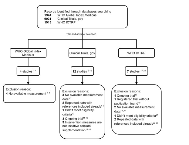
Figure 1. Flow chart of search and selection
References: 1. ID: emr-156089 (https://pesquisa.bvsalud.org/gim/resource/en/emr-156089) 2. ID: wpr-270003 (https://pesquisa.bvsalud.org/gim/resource/en/wpr-270003) 3. ID: lil-243754 (https://pesquisa.bvsalud.org/gim/resource/en/lil-243754) 4. ID: sea-23757 (https://pesquisa.bvsalud.org/gim/resource/en/sea-23757) 5. ID: NCT00067925 (https://clinicaltrials.gov/ct2/show/NCT00067925?term=NCT00067925&draw=2&rank=1) 6. ID: NCT00979511 (https://clinicaltrials.gov/ct2/show/NCT00979511?term=NCT00979511&draw=2&rank=1) 7. ID: NCT00065247 (https://clinicaltrials.gov/ct2/show/NCT00065247?term=NCT00065247&draw=2&rank=1) 8. Matkovic V, Landoll JD, Badenhop-Stevens NE, et al. Nutrition influences skeletal development from childhood to adulthood: a study of hip, spine, and forearm in adolescent females. J Nutr. 2004;134(3):701S-705S. doi:10.1093/jn/134.3.701S 9. Barger-Lux MJ, Davies KM, Heaney RP. Calcium supplementation does not augment bone gain in young women consuming diets moderately low in calcium. J Nutr. 2005;135(10):2362-2366. doi:10.1093/jn/135.10.2362 10. Cornes R, Sintes C, Peña A, et al. Daily Intake of a Functional Synbiotic Yogurt Increases Calcium Absorption in Young Adult Women. J Nutr. 2022;152(7):1647-1654. doi:10.1093/jn/nxac088 11. ID: NCT00063011 (https://clinicaltrials.gov/ct2/show/NCT00063011?term=NCT00063011&draw=2&rank=1) 12. ID: NCT00063024 (https://clinicaltrials.gov/ct2/show/NCT00063024?term=NCT00063024&draw=2&rank=1) 13. ID: NCT01857154 (https://clinicaltrials.gov/ct2/show/NCT01857154?term=NCT01857154&draw=2&rank=1) 14. ID: NCT00067600 (https://clinicaltrials.gov/ct2/show/NCT00067600?term=NCT00067600&draw=2&rank=1) 15. ID: NCT00063037 (https://clinicaltrials.gov/ct2/show/NCT00063037?term=NCT00063037&draw=2&rank=1) 16. ID: NCT00063050 (https://clinicaltrials.gov/ct2/show/NCT00063050?term=NCT00063050&draw=2&rank=1) 17. ID: TCTR20190624002 (https://trialsearch.who.int/Trial2.aspx?TrialID=TCTR20190624002) 18. ID: JPRN-UMIN000024182 (https://trialsearch.who.int/Trial2.aspx?TrialID=JPRN-UMIN000024182) 19. ID: NCT02636348 (https://trialsearch.who.int/Trial2.aspx?TrialID=NCT02636348) 20. ID: ACTRN 12612000374864 (https://trialsearch.who.int/Trial2.aspx?TrialID=ACTRN12612000374864) 21. ID: NCT01732328 (https://trialsearch.who.int/Trial2.aspx?TrialID=NCT01732328) 22. ID: ISRCTN28836000 (https://trialsearch.who.int/Trial2.aspx?TrialID=ISRCTN28836000) 23. ID: ISRCTN84437785 (https://trialsearch.who.int/Trial2.aspx?TrialID=ISRCTN84437785)
We have also updated the literature search section and the flow chart in the main text of the revised manuscript, as follows:
We applied search strategies to the following electronic bibliographic databases without language restrictions: PubMed, EMBASE, ProQuest, CENTRAL (Cochrane Central Register of Controlled Trials), WHO Global Index Medicus, Clinical Trials.gov, WHO ICTRP, China National Knowledge Infrastructure and Wanfang Data in April 2021 and updated the search in July 2022 for eligible studies addressing the effect of calcium or calcium supplementation, milk or dairy products with BMD or BMC as endpoints. (see Lines 80-85 on Page 5 and Figure 1 in the Main Text)
The manuscript compares two sources of participants (in line 233) evaluating the effect of improvements on the femoral neck being "obviously stronger in Western countries than in Asian countries". But, I didn't identify if the searches were conducted applying language restrictions. This is important because we can be considering the entire world or specific countries.
We are extremely grateful for your great patience and for your kind suggestions. We did not apply any language restrictions during the search process, as documented in the protocol of PROSPERO (CRD42021251275, https://www.crd.york.ac.uk/prospero/display_record.php?RecordID=251275). Following your suggestion, we have added a description of this in the revised manuscript. (See Lines 80-81 on Page 5 in the Main Text)
During the search process, we did identify five eligible articles from the Chinese databases including China National Knowledge Infrastructure (CNKI, https://www.cnki.net) and WanFang Data (https://www.wanfangdata.com.cn). However, we confirmed that these five studies were duplicates of the articles from the PubMed (PMID: 15230999; PMID: 17627404; PMID: 18296324; PMID: 20044757; PMID: 20460227). For those possibly relevant studies published in other languages than Chinese or English, the full text was downloaded and translated using DeepL translation website (https://www.deepl.com/translator) and then carefully reviewed. Ultimately, all included studies that met the inclusion and exclusion criteria were published in English. In view of this, after a systematic and comprehensive search, especially with the addition of your suggested databases, we could assume that our current study has incorporated all original researches in this field worldwide, rather than only from specific countries or regions.
To explore whether the effects of calcium supplementation differ across different population regions, we performed subgroup analyses. Prior to the analysis, we hypothesized that the effect might be slightly better, or at least not worse, in populations with lower baseline dietary calcium intakes (lower baseline BMD/BMC levels) than that in populations with higher baseline dietary calcium intakes (higher baseline BMD/BMC levels). However, the results showed that the improvement effects on BMD at the femoral neck and total body and BMC at the femoral neck and lumbar spine were obviously stronger in Western countries than in Asian countries. These findings are likely to be contrary to our common sense, which is, that under normal circumstances, the effects of calcium supplementation should be more obvious in people with lower calcium intakes than in those with higher calcium intakes. Therefore, this issue needs to be tested and confirmed in future trials.
The manuscript does not describe which version was used with the RoB tool.
Thank you for your suggestion. As you mentioned, we completed the description of RoB tool in the Methods section, as follows:
The quality of the included RCTs was assessed independently by two reviewers (SYL, HNJ) based on the Revised Cochrane Risk-of-Bias Tool for Randomized Trials (RoB 2 tool, version 22 August 2019), and each item was graded as low risk, high risk and some concerns. (See Lines 101-103 on Page 6 in the Main Text)
Figures and Supplementary: No critique.
Thanks for your kind comments and for your recognition to our work in this study.
Appendix 1
Search strategy • WHO Global Index Medicus:
(tw:(calcium)) OR (mj:(calcium)) OR (tw:(calcium carbonate)) OR (tw:(calcium citrate)) OR (tw:(calcium pills)) OR (tw:(calcium supplement)) OR (tw:(Ca2)) OR (tw:(dairy product)) OR (tw:(milk)) OR (tw:(yogurt)) OR (tw:(cheese)) OR (tw:(dietary supplement)) AND (tw:(bone density)) OR (tw:(bone mineral density)) OR (tw:(bone mineral content))
(calcium) OR (calcium supplementation) OR (milk) OR (dairy product) OR (yogurt) OR (cheese) Applied Filters: Interventional (clinical trial); Child (birth–17); Adult (18–64)
• WHO ICTRP
(calcium) OR (milk) OR (dairy) OR (yogurt) OR (cheese) in the Intervention
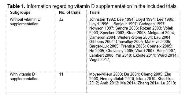
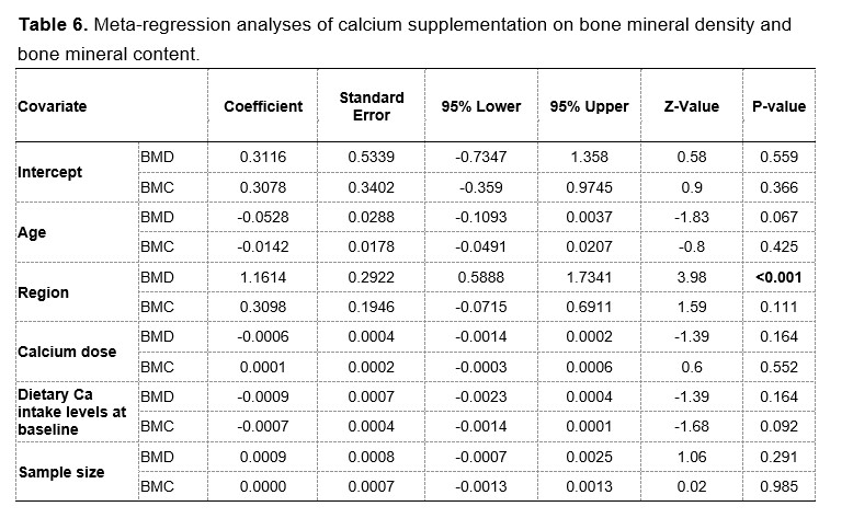
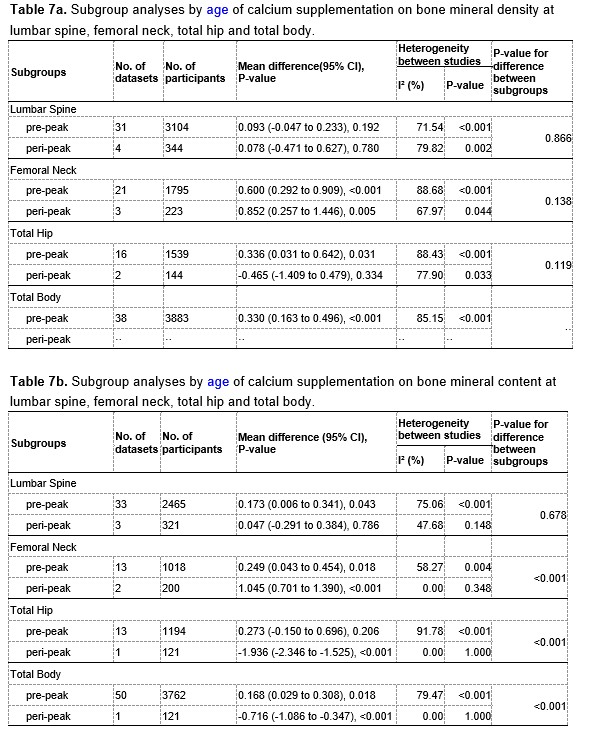
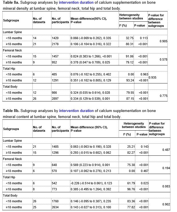
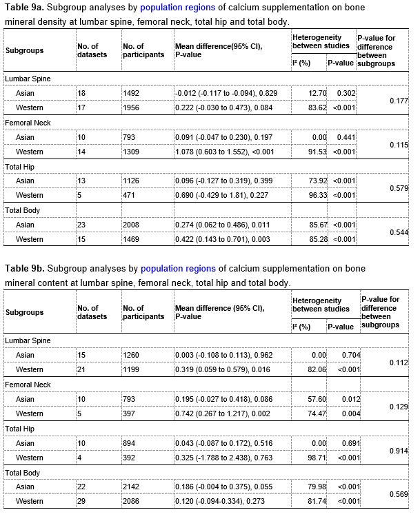
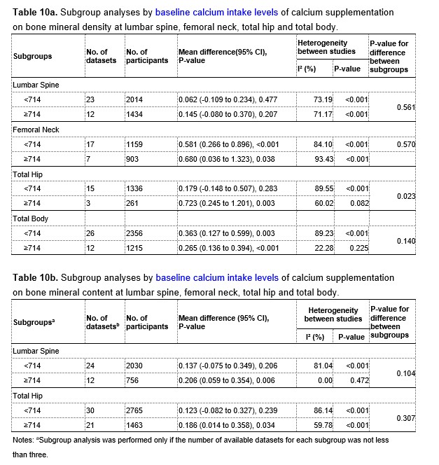
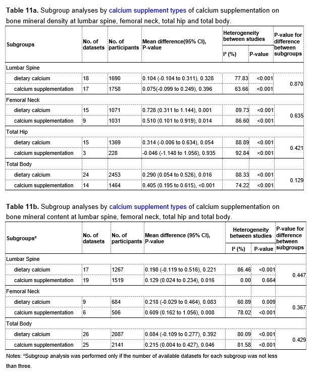
Author Response
Reviewer #2 (Public Review):
Zou et al. presented a comprehensive study where they generated single-cell RNA profiling of 138,982 cells from 13 samples of six patients including AK, squamous cell carcinoma in situ (SCCIS), cSCC, and their matched normal tissues, covering comprehensive clinical courses of cSCC. Using bioinformatics analysis, they identified keratinocytes, CAFs, immune cells, and their subpopulations. The authors further compared signatures within subpopulations of keratinocytes along with the clinical progression, especially basal cells, and identified many interesting genes. They also further validate some of the markers in an independent cohort using IHC, followed by some knockdown experiments using cSCC cell lines.
The strength of this study is the unique data set they have created, providing the community with invaluable resources to study and validate their findings. However, a lot of analyses were not robust enough to support the claims and conclusions in the paper. More clarification and cross-comparison with polished data are needed to further strengthen the study and claims.
1) Stemness markers were used. The authors used COL17A1, TP63, ITGB1, and ITGA3 to represent stemness markers. However, these were not common classic stemness markers used in cSCC. What is the source claiming these genes were stemness markers in cSCC? TP63 is a master regulator and early driver event in SCC, while COL17A1, ITGB1, and ITGA3 are all ECM genes. The authors need to use commonly well-known stem cell markers in cSCC, e.g., LGR5, to mark stem-like cells.
Thanks for raising this good point. We may not have provided a clear description of the markers COL17A1, TP63, ITGB1, and ITGA3 in the previous texts. We would like to clarify that these genes were used as the markers of epidermal stem cells in normal skin samples rather than tumor stem cells in cSCC. To avoid any possible misunderstanding, we revised the main text accordingly and added the references [4-11].
2) Cell proportion analysis. The authors used the mean proportions to compare different clinical groups for subpopulations of keratinocytes, e.g., Figure 2B, and Figure 5B. This is not robust, as no statistics can be derived from this. For example, from Fig 2A, it is clearly shown there is a high level of heterogeneity of cellular compositions for normal samples. One cannot say which group is higher or lower simply based on mean not variance as well.
We replotted the proportion analysis with statistics and presented the new graphs in Figure 2-figure supplement 1 for Figure 2B and Figure 5-figure supplement 1 for Figure 5B.
3) Basal tumour cells in SCCIS and SCC. To make the findings valid, authors need to compare these cells/populations with the keratinocyte cell populations defined by Ji et al. Cell 2020. Do basal-SCCIS-tumours cells, also in SCC samples, resemble any of the population defined in Ji et al. Ji et al. also had 10 match normal, thus the authors need to validate their findings of SCC vs normal analysis using the Ji et al. dataset.
Thanks for this valuable suggestion. We compared basal tumor cell in our study with the cell populations defined in Ji et al. Cell 2020 data using SingleCellNet [1]. The results showed that both the basal-SCCIS-tumor cells of SCCIS and basal tumor cells of cSCC in our study closely resemble the Tumor_KC_Basal subcluster defined in Ji et al’s paper (Figure 4-figure supplement 4, C and D). Tumor_KC_Basal highly expressed CCL2, CXCL14, FTH1, MT2A, which is consistent with our findings in basal tumor cells.
4) Copy number analysis. Authors used inferCNV to perform copy number analysis using scRNA-seq data and identified CNVs in subpopulations of keratinocytes in SCCIS and SCC. To ensure these CNVs were not artefacts, were some of the CNVs identified by inferCNV well-known copy number changes previously reported in cSCC?
In poorly-differentiated cSCC sample, the significant gains in chromosome 7, 9 and deletion in chromosome 10 were reported in previous study, indicating the reliability of the CNV analysis results (Figure 5-figure supplement 2) [12].
5) Pseudotime analysis lines 308-313. Not sure the pseudotime analysis added much as, as it is unclear two distinct subgroups were identified from this analysis. Suggest removing this to keep it neater
Thank you for this suggestion. We have deleted the result of pseudotime analysis.
6) Selection of candidate genes for validation using IHC and cell line work. For example, lines 205-206, lines 352-356 and lines 437-441, authors selected several genes associated with AK and SCC to further validate using IHC and cell line knockdown work. What are the criteria for selecting those genes for validation? It is unclear to readers how these were selected. It reads like a fishing experiment, then followed by a knockdown. Clear rationale/criteria need to be elaborated.
The first consideration of candidate gene selection is the fold change of expression. We have provided the statistical results of DEGs in Supplementary file 1b, 1h, 1j-1m. Then we selected top changed genes and conducted an extensive literature search on these genes. We prioritized genes that, although not directly associated with cSCC development, have a close relationship with related pathways, as determined through functional enrichment analysis. These genes were arranged for further verification experiments. We have added more details in main text and methods section.
7) TME. Compared to keratinocytes populations, the investigation of TME cells was weak. (a) can authors produce UMAP files just for T cells, DC cells, and fibroblasts separately? Figure 7B is not easy to see those subclusters. (b) similar to what was done for keratinocytes, can authors find differentially expressed clusters and genes among the different clinical groups, associated with disease progression? (c) where are the myeloid cell populations, also B cells?
Thank you for your suggestions. (a) We have added the UMAP files for T cells, DC cells and stromal cells separately in new Figure 7A. (b) We identified DEGs in TME cells among the different groups. Several key genes showed monotonically changing trends associated with disease progression. For example, with the increase of malignancy, FOS shows down-regulation while S100A8 and S100A9 monotonically increase in all three types of TME cells (Figure 7C). (c) We identified two types of myeloid cell populations, macrophage and monocyte derived DCs (MoDC). We didn’t find other myeloid cells, such as neutrophil. For B cells, there were only 28 B cells in poorly-differentiated cSCC sample, which didn’t meet the threshold for further cell-cell communication analysis.
8) Heat shock protein genes line 327-329. HSP signature was well-known to be induced via tissue dissociation and library prep during the scRNA experiment. How could the authors be sure these were not artefacts induced by the experiment? If authors regress their gene expression against HSP gene signatures, would this cluster still be identified?
Thank you for this valuable suggestion. It is important to note that the Basal-SCCIS-tumor cluster was identified through CNV analysis, rather than the HSP signature. To address this concern and further validate this result, “AddModuleScore” function in Seurat package was used to regress gene expression against HSP gene signatures for retrieved basal cells. Our result showed that Basal_SCCIS tumor population still can be identified after regression, even more clearly (Author response image 1).
Author response image 1.
The identity of Basal-SCCIS-tumor cluster considering regression against HSP signatures.
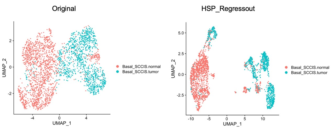
9) Cell-cell communication analysis. The authors claimed that that cell-to-cell interaction was significantly enhanced in poorly-differentiated cSCC, and multiple interaction pathways were significantly active. How was this kind of analysis carried out? How did the authors define significance? what statistical method was used? these were all unclear. Furthermore, it is difficult to judge the robustness of the cell-cell communication analysis. Were these findings also supported by another method, such as celltalker, and cellphoneDB?
To determine the significance of the increased overall cell-to-cell interaction strength between two groups, we utilized CellChat to obtain the communication strength in different samples. We combined the communication strength based on cell type pairs, where missing values were set to 0. We performed a paired Wilcoxon test to determine whether the enhancement of cell-to-cell interaction between samples was significant.
For the comparison of outgoing or incoming interaction strength of the same cell types between two groups, we first extracted the communication strength of each signal pathway contributing to outgoing or incoming strength, and then merged the strengths of signal pathways among samples, where the strength of non-shared pathways with missing value was determined to be 0. Subsequently, we performed a paired Wilcoxon test to define the significance.
For multiple groups comparisons, the Kruskal-Wallis rank sum test was first performed. If the p-value is less than 0.1, the pairwise Wilcoxon test was used for subsequent pairwise comparisons. The comparison of individual signaling pathways between groups is similar to the above. We defined p-value < 0.1 as significance threshold. We have added the significance test method in figure legend for Figure 7 and Figure 8 as well as and detailed statistical data in new Supplementary file 1q-1u.
As suggested, we also used the approach of CellPhoneDB based on CellChatDB database to verify our cell-cell communication results. There are 55-58% of the ligand-receptor interactions predicted by CellChat were also predicted by CellPhoneDB (Author response image 2). The enhancement of cell interaction through MHC-II, Laminin and TNF signaling pathways in poorly-differentiated cSCC sample compare to normal sample were consistent in both CellChat and CellPhoneDB (Figure 8C and Figure 8-figure supplement 1B).
Author response image 2.
The overlap of the predicted ligand-receptor interactions between CellChat and CellPhoneDB.
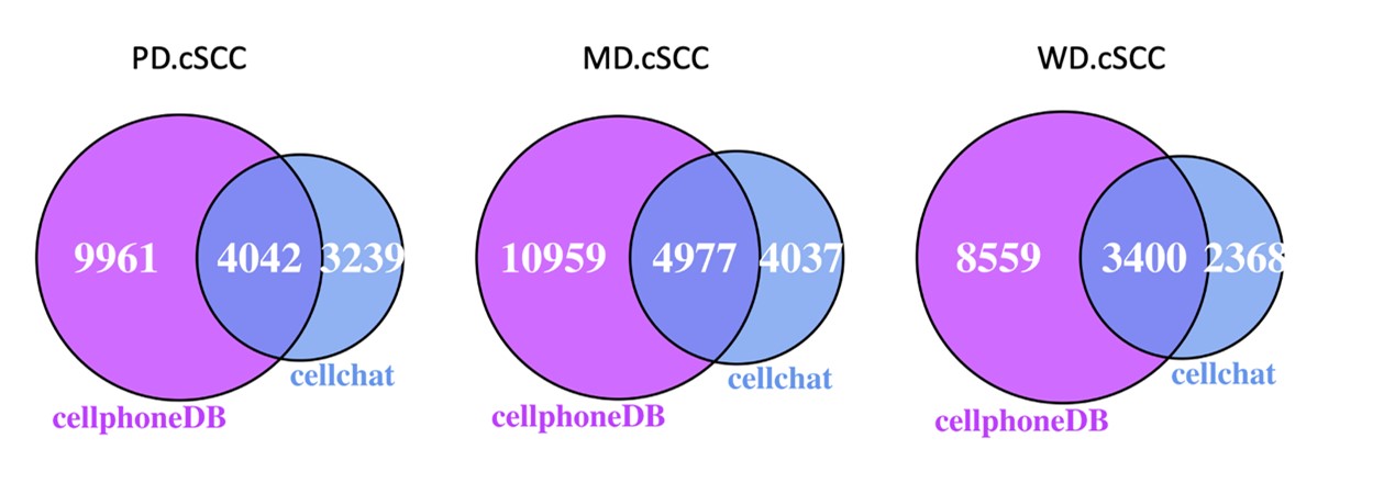
10) Statistics and significance. In general, the detail of statistics and significance was lacking throughout the paper. Authors need to specify what statistical tests were used, and the p-values. It is difficult to judge the correctness of the test, and robustness without seeing the stats.
We have included all statistics and significance values in the figure legend and supplemental tables, and described the statistical tests in the methods section. In this revision, we have added the necessary details of statistics and significance in the main text and figures.
11) Overall, this manuscript needs a lot of re-writing. A lot of discussion was also included in the results, making it really difficult to read overall. The authors should simplify the results sections, remove the discussion bits, and further highlight and streamline with the key results of this paper.
Thanks a lot for this advice. We have revised the paper thoroughly, removed discussion in results section to make the manuscript easier to read.
Author Response:
Reviewer #1 (Public Review):
5.The reported data point to an important role of the premotor and parietal regions of the left as compared to the right hemisphere in the control of ipsilateral and contralateral limb movements. These are also the regions where the electrodes were primarily located in both subgroups of patients. I have 2 concerns in this respect. The first concern refers to the specific locus of these electrodes. For premotor cortex, the authors suggest PMd as well as PMv as potential sites for these bilateral representations. The other principal site refers to parietal cortex but this covers a large territory. It would help if more specific subregions for the parietal cortex can be indicated, if possible. Do the focal regions where electrodes were positioned refer to the superior vs inferior parietal cortex (anterior or posterior), or intra-parietal sulcus. Second, the manuscript's focus on the premotor-parietal complex emerges from the constraints imposed by accessible anatomical locations in the participants but does not preclude the existence of other cortical sites as well as subcortical regions and cerebellum for such bilateral representations. It is meaningful to clarify this and/or list this as a limitation of the current approach.
On the first issue, we have updated the manuscript to specify the subregion within the parietal cortex in which we see stronger across-arm generalization - namely, the superior parietal cortex. On the second issue, we have added text in the Discussion that reference subcortical areas shown to exhibit laterality differences in bimanual coordination, providing a more holistic picture of bimanual representations across the brain. In addition, we acknowledge that with our current patient population we are limited to regions with substantial electrode coverage, which does not include all areas of the brain.
6.The evidence for bilateral encoding during unilateral movement opens perspectives for a better understanding of the control of bimanual movements which are abundant during every day life. In the discussion, the authors refer to some imaging studies on bimanual control in order to infer whether the obtained findings may be a consequence of left hemisphere specialization for bimanual movement control, leading to speculations about the information that is being processed for each of both limb movements. Another perspective to consider is the possibility that making a movement with one limb may require postural stabilization in the trunk and contralateral body side, including a contribution from the opposite limb that is supposedly resting on the start button. Have the authors considered whether this postural mechanism could (partly) account for this bilateral encoding mechanism, in particular, because it appears more prominent during movement execution as compared to preparation. Furthermore, could the prominence of bilateral encoding during movement execution be triggered by inflow of sensory information about both limbs from the visual as well as the somatosensory systems.
Thank you for these comments. We have added a paragraph to the Discussion to address the hypothesis that some component of ipsilateral encoding may be related to postural stabilization.
In response to the final point in this comment, we agree that bilateral information during execution could be reflective of afferent inputs (somatosensory and/or visual). However, the encoding model shows that activity in premotor and parietal regions are well predicted based on kinematics during the task. While visual and somatosensory system information are likely integrated in these areas, the kinematic encoding would point to a more movement-based representation.
Reviewer #2 (Public Review):
Weaknesses: 1. Although the current human ECoG data set is valuable, there is still large variability in electrode coverage across the patients (I fully acknowledge the difficulty). This makes statistical assessment a bit tricky. The potential factors of interest in the current study would be Electrode (=Region), Subject, Hemisphere, and their interactions. The tricky part is that Electrode is nested within Subject, and Subject is nested within Hemisphere. Permutation-based ANOVA used for the current paper requires proper treatment of these nested factors when making permutations (Anderson and Braak, 2003). With this regard, sufficient details about how the authors treated each factor, for instance, in each pbANOVA, are not provided in the current version of the manuscript. Similarly, the scope of statistical generalizability, whether the inference is within-sample or population-level, for the claims (e.g., statement about the hemispheric or regional difference) needs to be clarified.
We discuss at length the issue of electrode variability and have addressed this in the revised manuscript. Graphically, we have added a Supplemental Figure (S2). Statistically, we appreciate the point about the need for the analysis to address the nested structure of the data. We have redone all of the statistics, now using a permutation-based linear mixed effects model with a random effect of patient. This approach did not change any of the findings.
As to the comment about hemispheric or regional differences, the data show that both are important factors. Our hemispheric effect is characterized by stronger ipsilateral encoding in the left hemisphere and subsequently better across-arm generalization (Figures 2-4). We then examine the spatial distribution of electrodes that generalized well or poorly and found clusters in both hemispheres of electrodes that generalize poorly. In contrast, only in the left hemisphere did we find clusters of electrodes that generalize well. These electrodes were localized to PMd, PMv and superior parietal cortex (Fig 5D). In summary, we argue that activity patterns in M1 are similar in the left and right hemispheres, but there is a marked asymmetry for activity patterns over premotor and parietal cortices.
Additional contexts that would help readers interpret or understand the significance of the work: The greater amount of shared movement representation in the left hemisphere may imply the greater reliance of the left arm on the left hemisphere. This may, in turn, lead to the greater influence of the ongoing right arm motion on the left arm movement control during the bimanual coordination. Indeed, this point is addressed by the authors in the Discussion (page 15, lines 26-41). One critical piece of literature missing in this context is the work done by Yokoi, Hirashima, and Nozaki (2014). In the experiments using the bimanual reaching task, they in fact found that the learning by the left arm is to the greater degree influenced by the concurrent motion of the right arm than vice versa (Yokoi et al., J Neurosci, 2014). Together with Diedrichsen et al. (2013), this study will strengthen the authors' discussion and help readers interpret the present result of left hemisphere dominance in the context of more skillful bimanual action.
The Yokoi paper is a very important paper in revealing hemispheric asymmetries during skilled bimanual movements. However, we think it is problematic to link the hemispheric asymmetries we observe to the behavioral effects reported in the Yokoi paper (namely, that the nondominant, left arm was more strongly influenced by the kinematics of the right arm). One could hypothesize that the left hemisphere, given its representation of both arms, could be controlling both arms in some sort of direct way (and thus the action of the right arm will have an influence on left arm movement given the engagement of the same neural regions for both movements). It is also possible that the left hemisphere is receiving information about the state of both the right and left arms, and this underlies the behavioral asymmetry reported in Yokoi.
Reviewer #3 (Public Review):
In the present work, Merrick et al. analyzed ECoG recordings from patients performing out-and-back reaching movements. The authors trained a linear model to map kinematic features (e.g., hand speed, target position) to high frequency ECoG activity (HFA) of each electrode. The two primary findings were: 1) encoding strength (as assessed by held-out R2 values) of ipsilateral and contralateral movements was more bilateral in the left hemisphere than in the right and 2) across-arm generalization was stronger in the left hemisphere than in the right. As the authors point out in the Introduction, there are known 'asymmetries between the two hemispheres in terms of praxis', so it may not be surprising to find asymmetries in the kinematic encoding of the two hemispheres (i.e., the left hemisphere contributes 'more equally' to movements on either side of the body than the right hemisphere).
There is one point that I feel must be addressed before the present conclusions can be reached and a second clarification that I feel will greatly improve the interpretability of the results.
First, as is often the case when working with patients, the authors have no control over the recording sites. This led to some asymmetries in both the number of electrodes in each hemisphere (as the authors note in the Discussion) and (more importantly) in the location of the recording electrodes. Recording site within a hemisphere must be controlled for before any comparisons between the hemispheres can be made. For example, the authors note that 'the contralateral bias becomes weaker the further the electrodes are from putative motor cortex'. If there happen to be more electrodes placed further from M1 in the left hemisphere (as Supplementary Figure 1 seems to suggest), than we cannot know whether the results of Figures 2 and 3 are due to the left hemisphere having stronger bilateral encoding or simply more electrodes placed further from M1.
The reviewer makes a very valid point and this comment has led to our inclusion of a new Supplementary Figure, S2, in which we quantify the percentage of electrodes in each subregion.
Second, it would be useful if the authors provided a bit of clarification about what type of kinematic information the linear model is using to predict HFA. I believe the paragraph titled 'Target modulation and tuning similarity across arms' suggests that there is very little across-target variance in the HFA signal. Does this imply that the model is primarily ignoring the Phi and Theta (as well as their lagged counterparts) and is instead relying on the position and speed terms? How likely is it that the majority of the HFA activity around movement onset reflects a condition-invariant 'trigger signal' (Kaufman, et al., 2016). This trigger signal accounts for the largest portion of neural variance around movement onset (by far), and the weight of individual neurons in trigger signal dimensions tend to be positive, which means that this signal will be strongly reflected in population activity (as measured by ECoG). This interpretation does not detract from the present results in any way, but it may serve to clarify them.
To address this comment, we have added a new figure (Fig 6) which shows the relative contribution of each kinematic feature as well as their average weights across time for both contralateral and ipsilateral movements. This figure also addresses the reviewer’s question about the contribution of the target position to the model. As can be seen, features that reflect timing/movement initiation (position, speed) make a larger contribution compared to the two features which capture directional tuning (theta, phi). As the reviewer suggested, this result is in line Kaufman et al. (2016) which reported that a condition-invariant ‘trigger signal’ comprises the largest component of neural activity. We note that the target dependent features theta and phi still make a substantial contribution to the model (relative contribution: contra = 32%, ipsi = 37%). Previously, we have tested the contribution of the theta and phi features by comparing two models, one that only used position and speed (Movement model) and one that also included the two angular components phi and theta (Target Model). For a subset of electrodes, the held-out predictions were significantly better using the Target Model, a result we take as further evidence of electrode tuning within our dataset.
The figure below shows an electrode located in M1 that is tuned to targets when the patient reached with their contralateral arm as an example. We believe that having an explicit depiction of how the four features contribute to the HFA predictions will help the reader evaluate the model. These points are now addressed in the text in the results section discussing Figure 6.
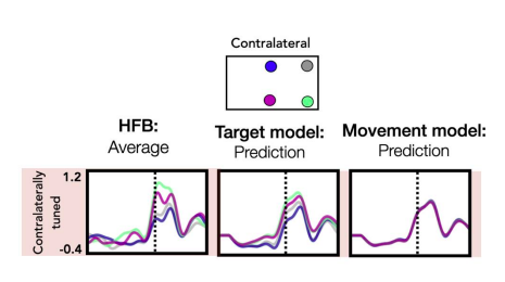
Author Response
Reviewer #3 (Public Review):
This manuscript by Pendse et al aimed to identify the role of the complement component C1q in intestinal homeostasis, expecting to find a role in mucosal immunity. Instead, however, they discovered an unexpected role for C1qa in regulating gut motility. First, using RNA-Seq and qPCR of cell populations isolated either by mechanical separation or flow cytometry, the authors found that the genes encoding the subunits of C1q are expressed predominantly in a sub-epithelial population of cells in the gut that Cd11b+MHCII+F4/80high, presumably macrophages. They support this conclusion by analyzing mice in which intestinal macrophages are depleted with anti-CSF1R antibody treatment and show substantial loss of C1qa, b and c transcripts. Then, they generate Lyz2Cre-C1qaflx/flx mice to genetically deplete C1qa in macrophages and assess the consequences on the fecal microbiome, transcript levels of cytokines, macromolecular permeability of the epithelial barrier, and immune cell populations, finding no major effects. Furthermore, provoking intestinal injury with chemical colitis or infection (Citrobacter) did not reveal macrophage C1qa-dependent changes in body weight or pathogen burden.
Then, they analyzed C1q expression by IHC of cross-sections of small and large intestine and find that C1q immunoreactivity is detectable adjacent to, but not colocalizing with, TUBB3+ nerve fibers and CD169+ cells in the submucosa. Interestingly, they find little C1q immunoreactivity in the muscularis externa. Nevertheless, they perform RNA-sequencing of LMMP preparations (longitudinal muscle with adherent myenteric plexus) and find a number of changes in gene ontology pathways associates with neuronal function. Finally, they perform GI motility testing on the conditional knockout mice and find that they have accelerated GI transit times manifesting with subtle changes in small intestinal transit and more profound changes in measures of colonic motility.
Overall, the manuscript is very well-written and the observation that macrophages are the major source of C1q in the intestine is well supported by the data, derived from multiple approaches. The observations on C1q localization in tissue and the strength of the conclusions that can be drawn from their conditional genetic model of C1qa depletion, however, would benefit from more rigorous validation.
1) Interpretation of the majority of the findings in the paper rest on the specificity of the Lyz2 Cre for macrophages. While the specificity of this Cre to macrophages and some dendritic cells has been characterized in the literature in circulating immune cells, it is not clear if this has been characterized at the tissue level in the gut. Evidence demonstrating the selectivity of Cre activity in the gut would strengthen the conclusions that can be drawn.
As indicated by the reviewer, Cre expression driven by the Lyz2 promoter is restricted to macrophages and some myeloid cells in the circulation (Clausen et al., 1999). To better understand intestinal Lyz2 expression at a cellular level, we analyzed Lyz2 transcripts from a published single cell RNAseq analysis of intestinal cells (Xu et al., 2019; see Figure below). These data show that intestinal Lyz2 is also predominantly expressed in gut macrophages with limited expression in dendritic cells and neutrophils.
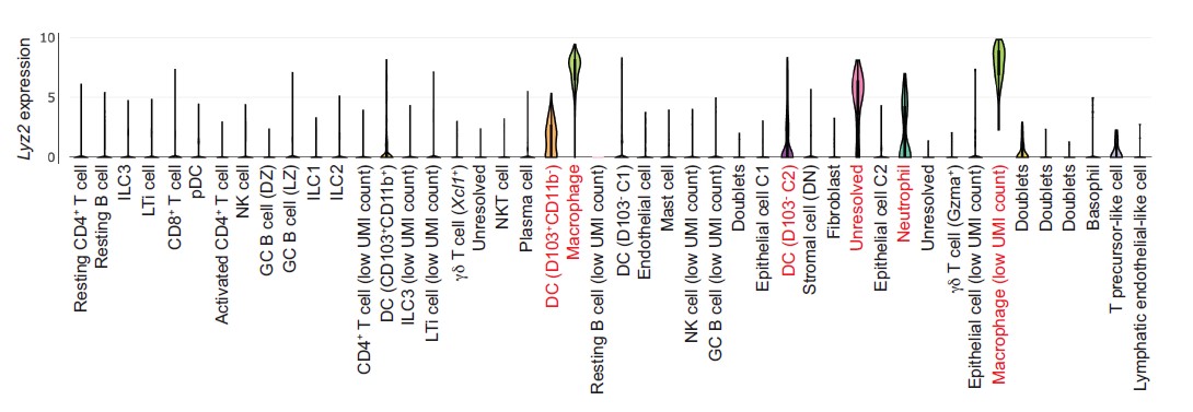
Figure. Lyz2 expression from single cell RNAseq analysis of mouse intestinal cells. Data are from Xu et al., Immunity 51, 696-708 (2019). Analysis was done through the Single Cell Portal, a repository of scRNAseq data at the Broad Institute.
Additionally, our study shows that intestinal C1q expression is restricted to macrophages (CD11b+MHCII+F4/80hi) and is absent from other gut myeloid cell lineages (Figure 1E-H). This conclusion is supported by our finding that macrophage depletion via anti-CSF1R treatment also depletes most intestinal C1q (Figure 2A-C). Importantly, we found that the C1qaDMf mice retain C1q expression in the central nervous system (Figure 2 – figure supplement 1). Thus, the C1qaDMf mice allow us to assess the function of macrophage C1q in the gut and uncouple the functions of macrophage C1q from those of C1q in the central nervous system.
2) Infectious and inflammatory colitis models were used to suggest that C1qa depletion in Lyz2+ lineage cells does not alter gut mucosal inflammation or immune response. However, the phenotyping of the mice in these models was somewhat cursory. For example, in DSS only body weight was shown without other typical and informative read-outs including colon length, histological changes, and disease activity scoring. Similarly, in Citrobacter only fecal cfu were measured. Especially if GI motility is accelerated in the KO mice, pathogen burden may not reflect efficiency of immune-mediated clearance alone.
We have added additional results which support our conclusion that C1qaDMf mice do not show a heightened sensitivity to acute chemically induced colitis. In Figure 3 – figure supplement 1 we now show a histological analysis of the small intestines of DSS-treated C1qafl/fl and C1qaΔMφ mice. This analysis shows that C1qaDMf mice have similar histopathology, colon lengths, and histopathology scores following DSS treatment. Likewise, our revised manuscript includes histological images of the colons of Citrobacter rodentium-infected C1qafl/fl and C1qaΔMφ mice showing similar pathology (Figure 3 – figure supplement 2).
3) The evidence for C1q expression being restricted to nerve-associated macrophages in the submucosal plexus was insufficient. Localization was shown at low magnification on merged single-planar images taken from cross-sections. The data shown in Figure 4C is not of sufficient resolution to support the claims made - C1q immunoreactivity, for example, is very difficult to even see. Furthermore, nerve fibers closely approximate virtually type of macrophage in the gut, from those in the lamina propria to those in the muscularis….Finally, the resolution is too low to rule out C1q immunoreactivity in the muscularis externa.
Similar points were raised by Reviewer 2. Our original manuscript claimed that C1q-expressing macrophages were mostly located near enteric neurons in the submucosal plexus but were largely absent from the myenteric plexus. However, as both Reviewers have pointed out, this conclusion was based solely on our immunofluorescence analysis of tissue cross-sections.
To address this concern we further characterized C1q+ macrophage localization by performing a flow cytometry analysis on macrophages isolated from the mucosa (encompassing both the lamina propria and submucosa) and the muscularis, finding similar levels of C1q expression in macrophages from both tissues (Figure 4 – figure supplement 1 in the revised manuscript). Although the mucosal macrophage fraction encompasses both lamina propria and submucosal macrophages, our immunofluorescence analysis (Figure 4 B and C) suggests that the mucosal C1q-expressing macrophages are mostly from the submucosal plexus. This observation is consistent with the immunofluorescence studies of CD169+ macrophages shown in Asano et al., which suggest that most C169+ macrophages are located in or near the submucosal region, with fewer near the villus tips (Fig. 1e, Nat. Commun. 6, 7802).
Most importantly, our flow cytometry analysis indicates that the muscularis/myenteric plexus harbors C1q-expressing macrophages. To further characterize C1q expression in the muscularis, we performed RNAscope analysis by confocal microscopy of the myenteric plexus from mouse small intestine and colon (Figure 4D). The results show numerous C1q-expressing macrophages positioned close to myenteric plexus neurons, thus supporting the flow cytometry analysis. We note that although the majority of C1q immunofluorescence in our tissue cross-sections was observed in the submucosal plexus, we did observe some C1q expression in the muscularis by immunofluorescence (Figure 4B and C). We have rewritten the Results section to take these new findings into account.
Is the 5um average on the proximity analysis any different for other macrophage populations to support the idea of a special relationship between C1q-expressing macrophages and neurons?
We agree that the proximity analysis lacks context and have therefore removed it from the figure. The other data in the figure better support the idea that C1q+ macrophages are found predominantly in the submucosal and myenteric plexuses and that they are closely associated with neurons at these tissue sites.
There are many vessels in the submucosa and many associated perivascular nerve fibers - could the proximity simply reflect that both cell types are near vessels containing C1q in circulation?
Our revised manuscript includes RNAscope analysis showing C1q transcript expression by macrophages that are closely associated with enteric neurons (Figure 4D). These findings support the idea that the C1q close to enteric neurons is derived from macrophages rather than from the circulation.
4) A major disconnect was between the observation that C1q expression is in the submucosa and the performance of RNA-seq studies on LMMP preparations. This makes it challenging to draw conclusions from the RNA-Seq data, and makes it particularly important to clarify the specificity of Lyz2-Cre activity.
Our revised manuscript provides flow cytometry data (Figure 4 – figure supplement 1) and RNAscope analysis (Figure 4D) showing that C1q is expressed in macrophages localized to the myenteric plexus. This accords with the results of our RNAseq analysis, which indicates altered LMMP neuronal function in C1qa∆Mφ mice (Figure 6A and B). Since neurons in the myenteric plexus are known to govern gut motility, it also helps to explain our finding that gut motility is accelerated in C1qa∆Mφ mice.
Finally, the pathways identified could reflect a loss of neurons or nerve fibers. No assessment of ENS health in terms of neuronal number or nerve fiber density is provided in either plexus.
Reviewers 1 and 2 also raised this point. Our revised manuscript includes a comparison of the numbers of enteric neurons in C1qafl/fl and C1qaΔMφ mice. There were no marked differences in neuron numbers in C1qaDMf mice when compared to C1qafl/fl controls (Figure 5A and B). There were also similar numbers of inhibitory (nitrergic) and excitatory (cholinergic) neuronal subsets and a similar enteric glial network (Figure 5C-E). Thus, our data suggest that the altered gut motility in the C1qaΔMφ mice arises from altered neuronal function rather than from an overt loss of neurons or nerve fibers. This conclusion is further supported by increased neurogenic activity of peristalsis (Figure 6H and I), and the expression of the C1q receptor BAI1 on enteric neurons (Figure 6 – figure supplement 4).
5) To my knowledge, there is limited evidence that the submucosal plexus has an effect on GI motility. A recent publication suggests that even when mice lack 90% of their submucosal neurons, they are well-appearing without overt deficits (PMID: 29666241). Submucosal neurons, however, are well known to be involved in the secretomotor reflex and fluid flux across the epithelium. Assessment of these ENS functions in the knockout mice would be important and valuable.
Our revised manuscript provides new data showing C1q expression by muscularis macrophages in the myenteric plexus. We analyzed muscularis macrophages by flow cytometry and found that they express C1q (Figure 4 – figure supplement 1). These findings are further supported by RNAscope analysis of C1q expression in wholemounts of LMMP from small intestine and colon (Figure 4D and E). These results are thus consistent with the increased CMMC activity and accelerated gut motility in the C1qaDMf mice. As suggested by the reviewer, our finding of C1q+ macrophages in the submucosal plexus indicates that C1q may also have a role controlling the function of submucosal plexus neurons. We are further exploring this idea through extensive additional experimentation. Given the expanded scope of these studies, we are planning to include them in a follow-up manuscript.
6) Immune function and GI motility can be highly sex-dependent - in all experiments mice of both sexes were reportedly used but it is not clear if sex effects were assessed.
This is a great point, and as suggested by the reviewer we indeed did encounter differences between male and female mice in our preliminary assays of gut motility. We therefore conducted our quantitative comparisons of gut motility between C1qafl/fl and C1qaDMf mice in male mice and now clearly indicate this point in the Materials and Methods.
Author Response
Reviewer #1 (Public Review):
This is a very interesting paper describing membrane potential dynamics of hippocampal principal cells during UP/DOWN transitions and sharp-wave ripples. Using whole-cell in combination with linear LFP recordings in head-fixed awake mice, the authors show striking differences of membrane potential responses in principal cells from the dentage gyrus, CA3 and CA1 sectors. The authors propose that switches between a dominant inhibitory excitable state and a disinhibited non-excitable state control the intra-hippocampal dynamics during UP/DOWN transitions.
Obtaining intracellular recordings in vivo is commendable. The authors provide valuable data and analysis. While data show clear trends and some of the conclusions are well supported, the authors may need to clarify the following potential confounds, which can actually impact their conclusions and interpretation:
1- All the analysis is based in z-scored membrane potential responses but the mean resting membrane potential is never reported. For DG granule cells recorded in awake conditions, the membrane potential is usually hyperpolarized so that most of the effect may be due to reversed GABAa mediated currents. Similarly, for those cells exhibiting the non-expected polarization during UP/DOWN states there may be drifts around reversal potentials explaining their behavior. Moreover, regional trends on passive and active membrane parameters and connectivity can actually explain part of the variability. A longitudinal comparison of state Vm and spikes in fig.5 suggests that some of the largest depolarized responses are not correlated with firing. Authors should evaluate this angle, ideally showing the distribution of membrane potential values across cells and regions and confronting this with the different membrane potential responses.
We added Figure 1 - figure supplement 4, which now describes the mean resting membrane potential, input resistance, burst propensity, and spikes per burst for the recorded cells. These data are provided in Figure 1 - source data 1 together with a recording identifier that can be used to link each cell to all other figure panels and data files. We further added Figure 1 - figure supplement 1, which provides examples of morphological information for our recordings, Figure 1 - figure supplement 2 that shows examples of bursts from morphologically identified neurons, and Figure 1 - figure supplement 3 that shows the locations of recorded cells.
In addition, we added Figure 5 - figure supplement 4 that includes the resting Vm and proximodistal location of cells in relation to their UP-DOWN modulation. We did not detect any significant trends with respect to brain state modulation. DG cells are more hyperpolarized compared to CA3 and CA1 cells and are closest to the reversal potential for GABAa (Figure 1 - figure supplement 4). The lack of any clear trends with respect to the resting Vm suggests that drifts around the GABAa reversal potential are unlikely to be a major factor driving variability in the observed UDS modulation.
2- While there are some trends for each hippocampal regions, there is also individual variability across cells during UP/DOWN transitions (fig.5) and near ripples (fig.6). What part of this variability can be explained by proximodistal and/or deep-superficial differences of cell location and identity? Can authors provide some morphological validation, even if in only a subset of cells? For CA3, proximodistal heterogeneity for intrinsic properties and entorhinal input responses are well documented in intracellular recordings both in vitro and in vivo. What is the location of CA3 cell contributing to this study? For CA1 cells, deep-superficial trends of GABAergic perisomatic inhibition and connectivity with input pathways dominate firing responses. Regarding DG cells, are all they from the upper blade?
We now provide morphological validation for a subset of cells (Figure 1 - figure supplement 1). Since we patch multiple cells in each experiment it is not possible to unequivocally determine their depth within the cell layer, although it is possible to confirm that they are granule cells or pyramidal cells in experiments where all labeled cells are principal neurons (Figure 1 - figure supplement 1). In addition, we added Figure 1 - figure supplement 3 that shows the proximodistal locations of recorded cells. With respect to the DG cells 20/22 are from the upper blade, with only two granule cells recorded in the lower blade (Figure 1 - figure supplement 3).
We added Figure 5 - figure supplement 4 that includes the resting Vm and proximodistal location of each cell as a function of UP-DOWN modulation. We did not detect any significant trends with respect to UDS modulation.
In addition, we added Figure 6 - figure supplement 1 that includes the resting Vm and proximodistal location of each cell as a function of ripple modulation. This figure shows that the most depolarized CA3 cells tend to hyperpolarize most during ripples, consistent with the fact that these cells are furthest away from the GABAa reversal potential and experience the highest driving force. No other significant trends were detected, although we would like to note that our recordings do not span the full proximodistal axis and may hence not be ideally suited to test the dependence of our results on proximodistal location.
3- AC-coupled LFP recordings cannot provide unambiguous identification of the sign of phasic CSD signals, because fluctuations accompanying UP/DOWN states alter the baseline reference. This is actually the case, given changes of membrane potential accompanying UP/DOWN transitions. I recommend reading Brankack et al. 1993 doi: 10.1016/0006-8993(93)90043-m. The authors should acknowledge this limitation and discuss how it could influence their results. One potential solution to get rid of this effect is using principal/independent component analysis for blind source separation.
We acknowledge the inherent limitations of AC-coupled recordings in regards to CSD analysis (Brankack et al., 1993). However, we do not believe these limitations affect our analysis or results for the reasons illustrated in Figure R1. Specifically, we do not attempt to measure the low frequency (< 1 Hz) CSD content directly. Instead, we extract the envelope of the rectified fast CSD transients. In the original submission we referred to this envelope signal as “DG CSD magnitude”, which may have been confusing. In the revised manuscript we use “DG CSD activity” instead to remove any suggestion that the low frequency CSD signal was directly measured. Notice that because of the rectification step the envelope signal is insensitive to the actual polarity of the fast transient CSD fluctuations. Using the envelope, we identify UP states as time periods when the rate and amplitude of EC input current transients, rather than the DC level, increases, in accordance with previous publications (Isomura et al., 2006). We further validated that the extracted UP/DOWN states reflect modulation of pupil diameter and ripple rate, quantities that are independently measured.
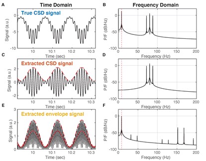
Figure R1. Deriving slow envelope signal from AC coupled recordings. (A) In this example the true CSD signal contains both a slow component (8 Hz) and a fast component (80 Hz) that is amplitude modulated by the slow component. Such phase-amplitude coupling is well known between theta and gamma oscillations in the hippocampus. The true CSD shows a current sink with time-varying magnitude. (B) The power spectral density (PSD) estimate of the signal in (A) shows both the slow (8 Hz) and fast (three peaks near 80 Hz) components. (C) Assume LFP recordings are obtained with a high-pass filter that has eliminated the slow component. Consequently, the estimated CSD signal contains only fast fluctuations. Furthermore, instead of a time-varying current sink it shows quickly alternating sinks and sources (both negative and positive values). The slow component can be visualized as the amplitude envelope (interrupted red line) of the signal. (D) PSD estimate shows that the slow component is absent from the extracted CSD signal. (E) Rectifying the CSD estimate (black) and then filtering (red) approximately recovers the true slow component (red interrupted). This is how the DG CSD activity signal is obtained. (F) PSD estimate of the rectified and filtered CSD signal recovers the slow component (interrupted red vertical line).
Reviewer #2 (Public Review):
In this manuscript "Inhibition is the hallmark of CA3 intracellular dynamics around awake ripples" the authors obtained Vm recordings from CA1, CA3 and DG neurons while also obtaining local field potentials across the CA1 and DG layers. This enabled them to identify periods of up and down state transitions, and to detect sharp-wave ripples (SWRs). Using these data, they then came to the conclusion that compared to CA1 and DG, the Vm of more CA3 neurons is hyperpolarized at the approximate time of SWRs.
Unfortunately, for the following reasons, the current manuscript does not necessarily support this conclusion:
Recordings are obtained in mice who are recently (same day) recovering from craniotomy surgery/anesthesia and have no training on head fixation. This means that the behavioral state is abnormal, and the animal may have residual anesthesia effects.
The main surgery for implanting the head-fixation apparatus and marking the coordinates for multisite and pipette insertion was carried out at least two days before the experiment. On the day of the experiment animals were briefly lightly anesthetized (<1 hr, at <1% isoflurane at 1 lit/min) for the sole purpose of resecting the dura at the two sites for multisite probe and pipette insertion. This procedure was carried out on the same day as the experiment in order to minimize the time the brain was exposed and optimize the quality of the recordings. Experiments began at least six hours after this short procedure. Furthermore, animals were given time to get familiarized with the behavioral apparatus before recordings began and showed no signs of distress.
Previous studies show that about 95% of isoflurane is eliminated within minutes by exhalation (Holaday et al., 1975). The further elimination of isoflurane proceeds with a fast phase with half-time of about 7-9 min and a slower phase with half-time of about 100-115 min (Chen et al., 1992), with the faster phase reflecting elimination from the brain (Litt et al., 1991). Given these considerations there should be negligible residual isoflurane from the short anesthesia six hours later when recordings are initiated.
In order to further investigate whether the short and light anesthesia during the day of recordings has any effect on the results reported in the paper, we carried out additional experiments in which we performed the surgery, including dura removal, 3 days before the recording session. The animals were habituated under head-fixation on the spherical treadmill for two hour periods each of the two days following the surgery. On the third day after surgery, we carried out recordings without any surgical procedures or anesthesia. The durations of UP and DOWN states without same day anesthesia were similar to those obtained in our previous experiments (Figure 2- figure supplement 4). The additional CA3 whole-cell recordings obtained in these new experiments have the same hyperpolarization features typical of our previous recordings. These additional experiments argue that the brief anesthesia on the day of recordings has no significant effect on the results.
Most of the paper is dedicated to dynamics around up-down state transitions, not focused on ripples.
We changed the title to “Up-Down states and ripples differentially modulate membrane potential dynamics across DG, CA3, and CA1 in awake mice” to reflect the analysis of both UP-DOWN state transitions and ripples. The two analyses are linked as the brain state modulation accounts for the slow Vm modulation around ripples.
Vm should be examined raw first, then split into fast and slow -the cell lives with the raw Vm.
The raw Vm can be obtained by adding the slow and fast Vm components. Hence the behavior of the Vm around ripples can be obtained by adding the panels of columns 1 and 3 in Figure 6. Decomposing into the slow and fast components illustrates how the slow modulation around ripples is due to brain state modulation of the slow component of the Vm (Figure 6).
While some (assumed) CA3 principal cells were hyperpolarized around the time of ripples, saying inhibition is the hallmark of CA3 dynamics around ripples is an exaggeration, especially because it does not seem mechanistically tied to anything else.
While a small fraction of CA3 cells is excited around ripples, the majority is inhibited. We suggest that the inhibition of the majority of CA3 neurons can account for the sparse and selective activation of CA3 around ripples.
The use of ripple onset time is questionable, since the detected onset of the ripple depends on the detector settings, amplifier signal-to-noise ratio, etc. The best and most widely used (including by a subset of these authors) metric is the ripple peak time.
We added Figure 6 - figure supplement 2, which shows that the Vm modulation around peak ripple power is the same as the modulation around ripple start, except for a small time shift due to the fact that the ripple power peaks shortly after ripple start. Our focus on ripple onset facilitates characterizing the timing of pre-ripple activity, such as the Vm depolarization observed before ripple onset for DG and CA1 neurons.
There is not enough raw data (or quality metrics) shown to judge the quality of the data, especially for the whole cell recordings. For instance what was the input resistance of the neurons? Was the access resistance constant?
We added Figure 1 - figure supplement 4, which now describes the mean resting membrane potential, input resistance, burst propensity, and spikes per burst for the recorded cells. These data are provided in Figure 1 - source data 1 together with a recording identifier that can be used to link each cell to all other figure panels and data files. We further added Figure 1- figure supplement 1, which provides examples of morphological information for our recordings, Figure 1 - figure supplement 2 that shows examples of bursts from morphologically identified neurons, and Figure 1 - figure supplement 3 that shows the locations of recorded cells.
There is not enough explanation regarding why the reported results on the spiking of CA1 and CA3 neurons in SWRs is so different than previously published. In general, whole cell recording is not the most reliable way to record spike timing, and the presented whole cell data differ from previously published juxtacellular and extracellular recording methods, which better preserve physiological spiking activity.
The CA1 neurons in this study depolarize and elevate their firing around ripples, consistent with previous intracellular and extracellular recordings. Our study reveals hyperpolarization of the majority of CA3 cells while only a small fraction is depolarized. This is consistent with the sparse activation of CA3 around ripples previously reported with extracellular studies. The overall firing rate change of CA3 neurons around ripples is a balance between the firing rate elevation of the small subset of activated cells and the net decrease in firing across the rest of the population. Since the baseline firing rate of CA3 pyramidal neurons in quiet wakefulness and sleep is low, the ripple-associated inhibition may not be readily observable in the spiking of individual CA3 neurons due to a “floor effect”. The overall rate of CA3 neurons we record increases before ripple onset, consistent with previous studies (Fig. 6D4). The subthreshold hyperpolarization of the majority of neurons provides novel insights into the mechanisms ensuring sparse and selective activation of the CA3 population around ripples.
The number of neurons from each area is not reported.
The number of cells was (indirectly) reported as the number of rows in Figs. 3-7. We now report the number of cells explicitly: 22 DG cells, 32 CA3 cells, and 32 CA1 cells.
There is no verification of cell type so it is inappropriate to assume that all neurons are the principal neurons.
We added Figure 1 - figure supplement 1, which shows morphological identification of recorded cells. We patch multiple cells in each experiment, but we can confirm the morphological identity of principal neurons when all stained cells have morphology of dentate granule cells or CA3/CA1 pyramidal neurons. The properties of morphologically identified cells in Figure 1 - figure supplement 1 are typical of all recorded cells (morphologically identified neurons from Figure 1 - figure supplement 1 are shown as diamonds in Figure 1- figure supplement 4, while the rest are shown as dots). There were no significant differences between the two groups (p > 0.05 t-test; p > 0.05 Wilcoxon rank sum test).
Are the fluctuations in the CA3 Vm generally smaller than for CA1 and DG because of physiology or technical reasons?
The recordings were done in exactly the same way across areas, arguing against technical reasons for any differences observed across the hippocampal subfields.
Reviewer #3 (Public Review):
During slow wave sleep and quiet immobility, communication between the hippocampus and the neocortex is thought to be important for memory formation notably during periods of hippocampal synchronous activity called sharp-wave ripple events. The cellular mechanisms of sharp-wave ripple initiation in the hippocampus are still largely unknown, notably during awake immobility. In this paper, the authors addressed this question using patch-clamp recordings of principal cells in different hippocampal subfields (CA3, CA1 and the dentate gyrus) combined with extracellular recordings in awake head-fixed mice as well as computer modeling. Using the current source density (CSD) profile of local field potential (LFP) recordings in the molecular layer of the dentate gyrus as a proxy of UP/DOWN state activity in the entorhinal cortex they report the preferential occurrence of sharp-wave ripple (recorded in area CA1) during UP states with a higher probability toward the end of the UP state (unlike eye blinks which preferentially occur during DOWN states). Patch-clamp recordings reveal that a majority of dentate granule cells get depolarized during UP state while a majority of CA3 pyramidal cells get hyperpolarized and CA1 pyramidal cells show a more mixed behavior. Closer examination of Vm behavior around state transitions revealed that CA3 pyramidal cells are depolarized and spike at the DOWN/UP transition (with some cells depolarizing even earlier) and then progressively hyperpolarize during the course of the UP state while DGCs and CA1 pyramidal cells tend to depolarize and fire throughout the UP state. Interestingly, CA3 pyramidal cells also tend to be hyperpolarized during ripples (except for a minority of cells that get depolarized and could be instrumental in ripple generation), while DGCs and CA1 pyramidal cells tend to be depolarized and fire. The strong activation of dentate granule cells during ripples is particularly interesting and deserves further investigations. The observation that the probability of ripple occurrence increases toward the end of the UP state, when CA3 pyramidal cells are maximally hyperpolarized, suggests that the inhibitory state of the CA3 hippocampal network could be permissive for ripple generation possibly by de-inactivation of voltage-gated channels thus increasing their excitability (i.e. ability to get excited). Altogether, these results confirm previous work on the impact of slow oscillations on the membrane potential of hippocampal neurons in vivo under anesthesia but also point to specificities possibly linked to the awake state. They also invite to revisit previous models derived from in vitro recordings attributing synchronous activity in CA3 to a global build-up of excitatory activity in the network by suggesting a role for Vm hyperpolarization in preserving the excitability of the CA3 network.
1) In light of recent report of heterogeneity within hippocampal cell types (and notably description of a new CA3 pyramidal cell type instrumental for sharp-wave ripple generation) (Hunt et al., 2018), the small minority of CA3 pyramidal cells depolarized during ripples deserve more attention. These cells are indeed likely key in the generation of sharp wave ripple. Several analyses could be performed in order to decipher whether they have specific intrinsic properties (baseline Vm, firing threshold, burst propensity), whether they are located in specific sub-areas of CA3 (a versus b, deep versus superficial) and whether they are distinctively modulated during UP/DOWN states.
Following the reviewer’s suggestion we now analyze the properties and UDS modulation of the CA3 neurons that are depolarized around ripples (Figure 6 - figure supplement 3). These neurons have comparable resting Vm, spike thresholds, and burst propensity as the rest of the CA3 population (p > 0.05, t-test). These CA3 cells had lower firing probability in the DOWN state. The locations of the depolarized cells are distributed across CA3c,b and are not clustered compared to the rest of the cells (Figure R2).
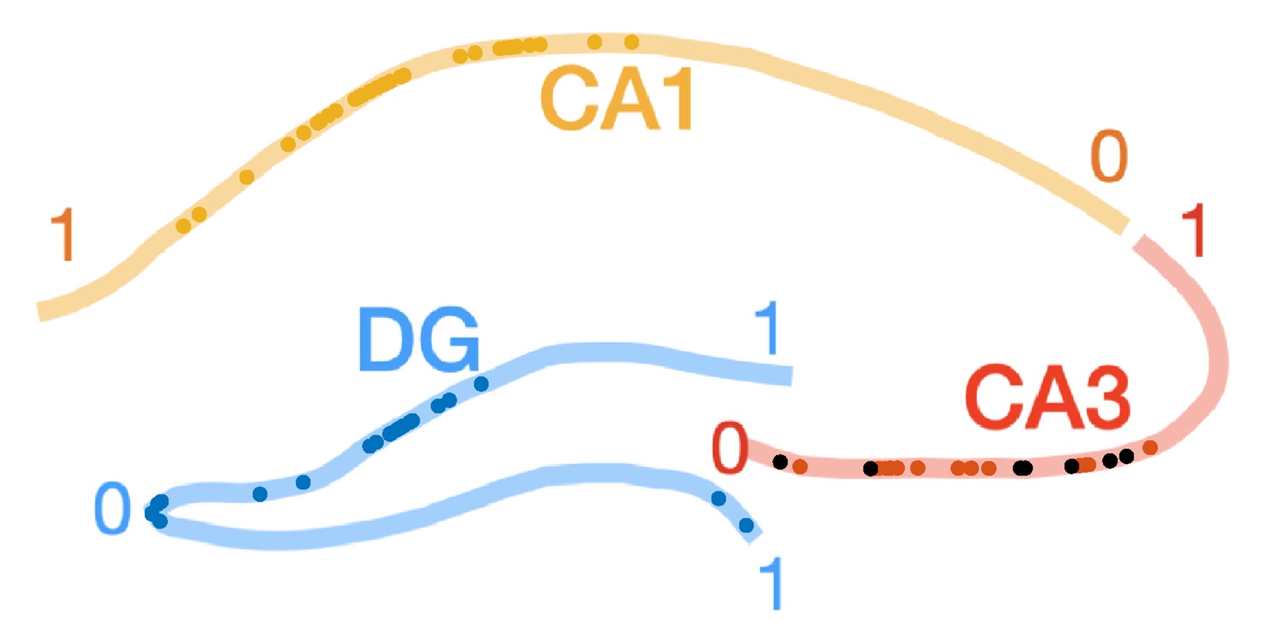
Figure R2. Proximodistal locations of CA3 cells that depolarize during ripples. Same as Figure 1 - figure supplement 3, but CA3 cells showing depolarization in their ripple-triggered average (RTA) response are marked with black dots. There was no significant difference in the proximodistal locations of these cells compared to the rest of the CA3 population (p > 0.05, t-test).
The population of athorny cells described in Hunt et al. represents a small percentage of CA3 cells (10-20%) that are concentrated in the CA3a region, which we do not sample in our recordings. Hence, the depolarized cells are unlikely to correspond to the athorny cells reported in Hunt et al.
2) The authors use CSD analysis in the DG as a proxy of synaptic inputs coming from the EC to define alternating periods of UP and DOWN states. I have few questions concerning this procedure: 1- It is unclear if only periods when animals was still/immobile were analyzed. 2- How coherent were these periods with slow oscillations recorded in the cortex (which are also recorded with the linear probe?).
The analysis was restricted to periods of immobility, which comprise the majority of the recording time as the animals are not performing any task. Cortical LFPs exhibit high coherence for low frequencies (<1 Hz) with the rectified DG CSD signal (Figure R3), although the contribution of volume conduction to this effect cannot be ruled out.
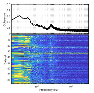
Figure R3. Coherence between DG CSD power and cortical LFP. (Top) population average magnitude squared coherence between DG CSD power (rectified CSD from the DG molecular layer) and cortical LFP across all recorded datasets. Notice the elevated coherence at low frequencies (< 1 Hz, vertical interrupted line) as well as the peak at theta ( 7-8 Hz). Volume conduction from other brain areas (i.e. the hippocampus) contributes to the cortical LFP and may be responsible for the coherence at theta, as well as at low frequencies. (Bottom) Each row in the pseudocolor image shows the coherence between DG CSD power and cortical LFP for a given dataset.
3- How long did these periods last? Did they occur during classically described hippocampal states (LIA/SIA) or do they correspond to a different state (Wolansky et al., J Neurosci 2006).
The distribution of UP and DOWN state durations is shown in Figure 2 - figure supplement 4.
We also added Figure 2 - supplementary figure 8 that shows the distribution of LIA and SIA transitions as a function of UDS phase. The LIA and SIA states were computed based on LFPs from CA1 stratum radiatum as described in (Hulse et al., 2017). The detected LIA→SIA transitions map very closely to UP→DOWN transitions. The SIA→LIA transitions are also concentrated around DOWN→UP transitions, but the distribution is broader compared to the LIA→SIA transitions. These observations are consistent with UP states broadly overlapping with LIA and DOWN states with SIA.
3) To better characterize hippocampal CSD profiles around ripples and UP/Down states transitions, could you plot ripple and UDS transition-triggered average CSD profiles across hippocampal subfields?
We added Figure 2 - supplementary figure 7 that shows average CSD profiles around UP/DOWN state transitions and ripples.
4) The duration of UP states appears longer than that reported in anesthetized animals. To ascertain this fact could the authors quantify and report mean UP and DOWN states durations? Shorter DOWN states would decrease the probability to detect ripple. Could the authors correct for this bias in their analysis of ripple occurrence during UP and DOWN states?
We report the medians and means of the distributions of UP and DOWN durations in Figure 2 - figure supplement 4. Ripples occur almost exclusively during the UP states, with almost no ripples occurring in DOWN states. Furthermore, the duration of UP and DOWN states is comparable suggesting that the duration of DOWN states does not bias the probability of ripple detection. We also added Figure 2 - figure supplement 2B, showing the rate (in Hz) of ripple occurrence as a function of UDS phase, which explicitly controls for UDS phase occupancy.
The duration of UP and DOWN states in quiet wakefulness depend on the behavior of the animal, attentional state, and external stimuli and need not be the same as in anesthesia or sleep when the animal is not behaving and is less responsive to external stimuli. To provide validation that the extracted UP and DOWN states in quiet wakefulness indeed correspond to genuine brain states, we show that the pupil diameter and ripple rates which are independently extracted are strongly modulated around the extracted UP and DOWN states.
5) The authors report a high coherence between the Vm of an example CA3 pyramidal cells and UP/DOWN state in DG. Was it a general property of a majority of CA3 pyramidal cells? The coherence values should be reported for all CA3 pyramidal cells.
We added Figure 2 - figure supplement 1, which reports the coherence of all cells across the subfields with the rectified DG CSD. The coherence values are similar across cells and subfields. We also report correlations between the slow component of the Vm and DG CSD activity for all cells in Figure 3. Neurons in CA3 exhibit negative correlations in contrast to DG and CA1, with the absolute values of the correlations similar across the subfields.
6) Was the high coherence between DG CSD magnitude and CA3 Vm specific to these slow oscillatory periods or a more general feature of the DG/CA3 functional coupling. For example, was it also observed during theta/movement periods?
Figure 2 - figure supplement 1 reports the coherence of all cells across the subfields with rectified DG CSD over the entire recording duration. Mice do not perform any tasks during the recordings so periods of immobility and quiet wakefulness comprise the majority of the recording session and are the focus of our analysis. During some occasional theta periods there is increased coherence in the theta frequency band (figure R4).
7) Fig. 6 shows depolarization and increase firing in DGCs up to 150 ms prior to ripple onset. However, ripples sometime occur in bursts with one ripple following others. Could such phenomenon explain the firing prior to ripples? (which would in fact correspond to firing during a previous ripple). What is the behavior of firing rate and Vm of different cells types if analysis is restricted to isolated ripples? This analysis is notably important in CA3 where feedback inhibition following a first ripple could lead to hyperpolarization « during » the next ripple.
We added a new figure (Figure 7 - figure supplement 2) that compares Vm aligned to the onset of isolated single ripples vs. ripple doublets. The pre-ripple depolarization in DG and CA1 is similar for isolated ripples and ripple doublets arguing against the hypothesis that pre-ripple responses are a reflection of ripple bursts.
Author Response
Reviewer #1 (Public Review):
The manuscript by Royall et al. builds on previous work in the mouse that indicates that neural progenitor cells (NPCs) undergo asymmetric inheritance of centrosomes and provides evidence that a similar process occurs in human NPCs, which was previously unknown.
The authors use hESC-derived forebrain organoids and develop a novel recombination tag-induced genetic tool to birthdate and track the segregation of centrosomes in NPCs over multiple divisions. The thoughtful experiments yield data that are concise and well-controlled, and the data support the asymmetric segregation of centrosomes in NPCs. These data indicate that at least apical NPCs in humans undergo asymmetric centrosome inheritance. The authors attempt to disrupt the process and present some data that there may be differences in cell fate, but this conclusion would be better supported by a better assessment of the fate of these different NPCs (e.g. NPCs versus new neurons) and would support the conclusion that younger centriole is inherited by new neurons.
We thank the reviewer for their supportive comments (“…thoughtful experiments yield data that are concise and well-controlled…”).
Reviewer #2 (Public Review):
Royall et al. examine the asymmetric inheritance of centrosomes during human brain development. In agreement with previous studies in mice, their data suggest that the older centrosome is inherited by the self-renewing daughter cell, whereas the younger centrosome is inherited by the differentiating daughter cell. The key importance of this study is to show that this phenomenon takes place during human brain development, which the authors achieved by utilizing forebrain organoids as a model system and applying the recombination-induced tag exchange (RITE) technology to birthdate and track the centrosomes.
Overall, the study is well executed and brings new insights of general interest for cell and developmental biology with particular relevance to developmental neurobiology. The Discussion is excellent, it brings this study into the context of previous work and proposes very appealing suggestions on the evolutionary relevance and underlying mechanisms of the asymmetric inheritance of centrosomes. The main weakness of the study is that it tackles asymmetric inheritance only using fixed organoid samples. Although the authors developed a reasonable mode to assign the clonal relationships in their images, this study would be much stronger if the authors could apply time-lapse microscopy to show the asymmetric inheritance of centrosomes.
We thank the reviewer for their constructive and supportive comments (“…the study is well executed and brings new insights of general interest for cell and developmental biology with particular relevance to developmental neurobiology….”). We understand the request for clonal data or dynamic analyses in organoids (e.g., using time-lapse microscopy). We also agree that such data would certainly strengthen our findings. However, as outlined above (please refer to point #1 of the editorial summary), this is unfortunately currently not feasible. However, we have explicitly discussed this shortcoming in our revised manuscript and why future experiments (with advanced methodology) will have to do these experiments.
Reviewer #3 (Public Review):
In this manuscript, the authors report that human cortical radial glia asymmetrically segregates newly produced or old centrosomes after mitosis, depending on the fate of the daughter cell, similar to what was previously demonstrated for mouse neocortical radial glia (Wang et al. 2009). To do this, the authors develop a novel centrosome labelling strategy in human ESCs that allows recombination-dependent switching of tagged fluorescent reporters from old to newly produced centrosome protein, centriolin. The authors then generate human cortical organoids from these hESCs to show that radial glia in the ventricular zone retains older centrosomes whereas differentiated cells, i.e. neurons, inherit the newly produced centrosome after mitosis. The authors then knock down a critical regulator of asymmetric centrosome inheritance called Ninein, which leads to a randomization of this process, similar to what was observed in mouse cortical radial glia.
A major strength of the study is the combined use of the centrosome labelling strategy with human cortical organoids to address an important biological question in human tissue. This study is similarly presented as the one performed in mice (Wang et al. 2009) and the existence of the asymmetric inheritance mechanism of centrosomes in another species grants strength to the main claim proposed by the authors. It is a well-written, concise article, and the experiments are well-designed. The authors achieve the aims they set out in the beginning, and this is one of the perfect examples of the right use of human cortical organoids to study an important phenomenon. However, there are some key controls that would elevate the main conclusions considerably.
We thank the reviewer for their overall support of our findings (“..authors achieve the aims they set out in the beginning, and this is one of the perfect examples of the right use of human cortical organoids to study an important phenomenon…”). We also understand the reviewer’s request for additional experiments/controls that “…would elevate the main conclusions considerably.”
1) The lack of clonal resolution or timelapse imaging makes it hard to assess whether the inheritance of centrosomes occurs as the authors claim. The authors show that there is an increase in newly made non-ventricular centrosomes at a population level but without labelling clones and demonstrating that a new or old centrosome is inherited asymmetrically in a dividing radial glia would grant additional credence to the central conclusion of the paper. These experiments will put away any doubt about the existence of this mechanism in human radial glia, especially if it is demonstrated using timelapse imaging. Additionally, knowing the proportions of symmetric vs asymmetrically dividing cells generating old/new centrosomes will provide important insights pertinent to the conclusions of the paper. Alternatively, the authors could soften their conclusions, especially for Fig 2.
We understand the reviewer’s request. As outlined above (please refer to point #1 of the editorial summary), we had tried previously to add data using single cell timelapse imaging. However, due to the size and therefore weakness of the fluorescent signal we had failed despite extensive efforts. According to the reviewer’s suggestion we have now explicitly discussed this shortcoming and softened our conclusions.
2) Some critical controls are missing. In Fig. 1B, there is a green dot that does not colocalize with Pericentrin. This is worrying and providing rigorous quantifications of the number of green and tdTom dots with Pericentrin would be very helpful to validate the labelling strategy. Quantifications would put these doubts to rest. Additionally, an example pericentrin staining with the GFP/TdTom signal in figure 4 would also give confidence to the reader. For figure 4, having a control for the retroviral infection is important. Although the authors show a convincing phenotype, the effect might be underestimated due to the incomplete infection of all the analyzed cells.
We have included more rigorous quantifications in our revised manuscript.
For Figure 1: There are indeed some green speckles that might be misinterpreted as a green centrosome. However, the speckles are usually smaller and by applying a strict size requirement we exclude speckles. To check whether the classifier might interpret any speckles as centrosomes, we manually checked 60 green “dots” that were annotated as centrosome. From these images all green spots detected as centrosome co-localized with Pericentrin signal (Images shown in Author response image 1).
For Figure 4: as we are comparing cells that were either infected with a retrovirus expressing scrambled or Ninein-targeting shRNA we compare cells that experienced a similar treatment. Besides that, only cells infected with the virus express Cre-ERT2 whereby only the centrosomes of targeted cells were analyzed. Accordingly, we only compare cells expressing scrambled or Ninein-targeting shRNA, all surrounding “wt” cells are not considered.
Author response image 1.
Pictures used to test the classifier. Each of the green “dots” recognized by the classifier as a Centriolin-NeonGreen-containing centrosome (green) co-localized with Pericentrin signal (white).
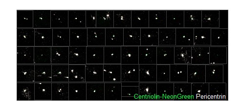
3) It would be helpful if the authors expand on the presence of old centrosomes in apical radial glia vs outer radial glia. Currently, in figure 3, the authors only focus on Sox2+ cells but this could be complemented with the inclusion of markers for outer radial glia and whether older centrosomes are also inherited by oRGCs. This would have important implications on whether symmetric/asymmetric division influences the segregation of new/old centrosomes.
That is an interesting question and we do agree that additional analyses, stratified by ventricular vs. oRGCs would be interesting. However, at the time points analysed there are only very few oRGCs present (if any) in human ESC-derived organoids (Qian et al., Cell, 2016). However, we have now added this point for future experiments to our discussion.
Author Response
Reviewer #1 (Public Review):
[...] Recently, pupil dilation was linked to cholinergic and noradrenergic neuromodulation as well as cortical state dynamics in animal research. This work adds substantially to this growing research field by revealing the temporal and spatial dynamics of pupil-linked changes in cortical state in a large sample of human participants.
The analyses are thorough and well conducted, but some questions remain, especially concerning unbiased ways to account for the temporal lag between neural and pupil changes. Moreover, it should be stressed that the provided evidence is of indirect nature (i.e., resting state pupil dilation as proxy of neuromodulation, with multiple neuromodulatory systems influencing the measure), and the behavioral relevance of the findings cannot be shown in the current study.
Thank you for your positive feedback and constructive suggestions. We are especially grateful for the numerous pointers to other work relevant to our study.
- Concerning the temporal lag: The authors' uniformly shift pupil data (but not pupil derivative) in time for their source-space analyses (see above). However, the evidence for the chosen temporal lags (930 ms and 0 ms) is not that firm. For instance, in the cited study by Reimer and colleagues [1] , cholinergic activation shows a temporal lag of ~ 0.5 s with regard to pupil dilation - and the authors would like to relate pupil time series primarily to acetylcholine. Moreover, Joshi and colleagues [2] demonstrated that locus coeruleus spikes precede changes in the first derivative of pupil dilation by about 300 ms (and not 0 ms). Finally, in a recent study recording intracranial EEG activity in humans [3], pupil dilation lagged behind neural events with a delay between ~0.5-1.7s. Together, this questions the chosen temporal lags.
More importantly, Figures 3 and S3 demonstrate variable lags for different frequency bands (also evident for the pupil derivative), which are disregarded in the current source-space analyses. This biases the subsequent analyses. For instance, Figure S3 B shows the strongest correlation effect (Z~5), a negative association between pupil and the alpha-beta band. However, this effect is not evident in the corresponding source analyses (Figure S5), presumably due to the chosen zero-time-lag (the negative association peaked at ~900 ms)).
As the conducted cross-correlations provided direct evidence for the lags for each frequency band, using these for subsequent analyses seems less biased.
This is an important point and we gladly take the opportunity to clarify this in detail. In essence, choosing one particular lag over others was a decision we took to address the multi-dimensional issue of presenting our results (spectral, spatial and time dimensions) and fix one parameter for the spatial description (see e.g. Figure 4). It is worth pointing out first that our analyses were all based on spectral decompositions that necessarily have limited temporal resolutions. Therefore, any given lag represents the center of a band that we can reasonably attribute to a time range. In fact, Figure 3C shows how spread out the effects are. It also shows that the peaks (troughs) of low and high frequency ranges align with our chosen lag quite well, while effects in the mid-frequency range are not “optimally” captured.
As picking lags based on maximum effects may be seen as double dipping, we note that we chose 0.93 sec a priori based on the existing literature, and most prominently based on the canonical impulse response of the pupil to arousing stimuli that is known to peak at that latency on average (Hoeks & Levelt, 1993; Wierda et al. 2012; also see Burlingham et al.; 2021). This lag further agrees with the results of reference [3] cited by the reviewer as it falls within that time range, and with Reimer et al.’s finding (cited as [1] above), as well as Breton-Provencher et al. (2019) who report a lag of ~900 ms sec (see their Supplementary Figure S8) between noradrenergic LC activation and pupil dilation. Finally, note that it was not our aim to relate pupil dilations to either ACh or NE in particular as we cannot make this distinction based on our data alone. Instead, we point out and discuss the similarities of our findings with time lags that have been reported for either neurotransmitter before.
With respect to using different lags, changing the lag to 0 or 500 msec is unlikely to alter the reported effects qualitatively for low- and high frequency ranges (see Figure 3C), as both the pupil time series as well as fluctuations in power are dominated by very slow fluctuations (<< 1 Hz). As a consequence, shifting the signal by 500 msec has very little impact. For comparison, below we provide the reviewer with the results presented in Figure 4 but computed based on zero (Figure R1) and 500-msec (Figure R2) lags. While there are small quantitative differences, qualitatively the results remain mostly identical irrespective of the chosen lag.
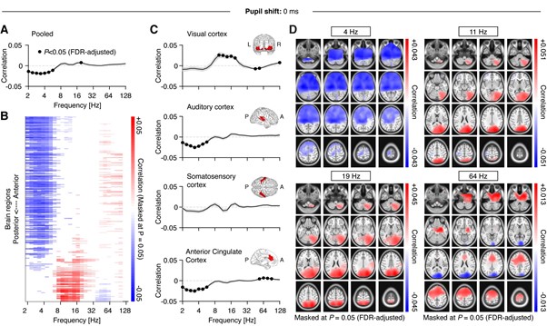
Figure R1. Figure equivalent to main Figure 4, but without shifting the pupil.
In sum, choosing one common lag a priori (as we did here) does not necessarily impose more of a bias on the presentation of the results than choosing them post-hoc based on the peaks in the cross-correlograms. However, we have taken this point as a motivation to revise the Results and Methods sections where applicable to strengthen the rationale behind our choice. Most importantly, we changed the first paragraph that mentions and justifies the shift as follows, because original wording may have given the false impression that the cross-correlation results influenced lag choice:
“Based on previous reports (Hoeks & Levelt, 1993; Joshi et al., 2016; Reimer et al., 2016), we shifted the pupil signal 930 ms forward (with respect to the MEG signal). We introduced this shift to compensate for the lag that had previously been observed between external manipulations of arousal (Hoeks & Levelt, 1993) as well as spontaneous noradrenergic activity (Reimer et al., 2016) and changes in pupil diameter. In our data, this shift also aligned with the lags for low- and high-frequency extrema in the cross-correlation analysis (Figure 3B).”
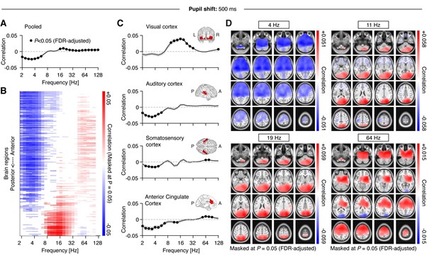
Figure R2. Figure equivalent to main Figure 4, but with shifting the pupil with respect to the MEG by 500 ms.
Related to this aspect: For some parts of the analyses, the pupil time series was shifted with regard to the MEG data (e.g., Figure 4). However, for subsequent analyses pupil and MEG data were analyzed in concurrent 2 s time windows (e.g., Figure 5 and 6), without a preceding shift in time. This complicates comparisons of the results across analyses and the reasoning behind this should be discussed.
The signal has been shifted for all analyses that relate to pupil diameter (but not pupil derivative). We have added versions of the following statement in the respective Results and Methods section to clarify (example from Results section ‘Nonlinear relations between pupil-linked arousal and band-limited cortical activity’):
“In keeping with previous analyses, we shifted the pupil time series forward by 930 msec, while applying no shift to the pupil derivative.”
- The authors refer to simultaneous fMRI-pupil studies in their background section. However, throughout the manuscript, they do not mention recent work linking (task-related) changes in pupil dilation and neural oscillations (e.g., [4-6]) which does seem relevant here, too. This seems especially warranted, as these findings in part appear to disagree with the here-reported observations. For instance, these studies consistently show negative pupil-alpha associations (while the authors mostly show positive associations). Moreover, one of these studies tested for links between pupil dilation and aperiodic EEG activity but did not find a reliable association (again conflicting with the here-reported data). Discussing potential differences between studies could strengthen the manuscript.
We have added a discussion of the suggested works to our Discussion section. We point out however that a recent study (Podvalny et al., https://doi.org/10.7554/eLife.68265) corroborates our finding while measuring resting-state pupil and MEG simultaneously in a situation very similar to ours. Also, we note that Whitmarsh et al. (2021) (reference [6]) is actually in line with our findings as we find a similar negative relationship between alpha-range activity in somatomotor cortices and pupil size.
Please also take into account that results from studies of task- or event-related changes in pupil diameter (phasic responses) cannot be straightforwardly compared with the findings reported here (focusing on fluctuations in tonic pupil size) , due to the inverse relationship between tonic (or baseline) and phasic pupil response (e.g. Knapen et al., 2016). This means that on trials with larger baseline pupil diameter, phasic pupil dilation will be smaller and vice versa. Hence, a negative relation between the evoked change in pupil diameter and alpha-band power can very well be consistent with the positive correlation between tonic pupil diameter and alpha-band activity that we report here for visual cortex.
In section ‘Arousal modulates cortical activity across space, time and frequencies’ we have added:
“Seemingly contradicting the present findings, previous work on task-related EEG and MEG dynamics reported a negative relationship between pupil-linked arousal and alpha-range activity in occipito-parietal sensors during visual processing (Meindertsma et al, 2017) and fear conditioning (Dahl et al. 2020).Note however that results from task-related experiments, that focus on evoked changes in pupil diameter rather than fluctuations in tonic pupil size, cannot be directly compared with our findings. Similar to noradrenergic neurons in locus coeruleus (Aston-Jones & Cohen, 2005), phasic pupil responses exhibit an inverse relationship with tonic pupil size (Knapen et al., 2016). This means that on trials with larger baseline pupil diameter (e.g. during a pre-stimulus period), the evoked (phasic) pupil response will be smaller and vice versa. As a consequence, a negative correlation between alpha-band activity in the visual cortex and task-related phasic pupil responses does not preclude a positive correlation with tonic pupil size during baseline or rest as reported here. In line with this, Whitmarsh et al., 2021 found a negative relationship between alpha-activity and pupil size in the somatosensory cortex that agrees with our finding. Although using an event-related design to study attention to tactile stimuli, this relationship occurred in the baseline, i.e. before observing any task-related phasic effects on pupil-linked arousal or cortical activity.”
In section ‘Arousal modulation of cortical excitation-inhibition ratio’ we have added: “The absence of this effect in visual cortices may explain why Kosciessa et al. (2021) found no relationship between pupil-linked arousal and spectral slope when investigating phasic pupil dilation in response to a stimulus during visual task performance. However, this behavioral context, associated with different arousal levels, likely also changes E/I in the visual cortex when compared with the resting state (Pfeffer et al., 2018).”
Finally, in the Conclusion we added (note: ‘they’ = the present results): “Further, they largely agree with similar findings of a recent independent report (Podvalny et al., 2021).”
Related to this aspect: The authors frequently relate their findings to recent work in rodents. For this it would be good to consider species differences when comparing frequency bands across rodents and primates (cf. [7,8]).
Throughout our Results section we have mainly remained agnostic with respect to labeling frequency ranges when drawing between-species comparisons, and have only reverted to it as a justification for a dimension reduction for some of the presented analysis. Following your comment however, we have phrased the following section in the Discussion, section ‘Arousal modulates cortical activity across space, time and frequencies’, more carefully:
“The low-frequency regime referred to in rodent work (2—10Hz; e.g., McGinley et al., 2015) includes activity that shares characteristics with human alpha rhythms (3—6Hz; Nestogel and McCormick, 2021; Senzai et al. 2019). The human equivalent however clearly separates from activity in lower frequency bands and,here, showed idiosyncratic relationships with pupil-linked arousal.”
- Figure 1 highlights direct neuromodulatory effects in the cortex. However, seminal [9-11] and more recent work [12,13] demonstrates that noradrenaline and acetylcholine also act in the thalamus which seems relevant concerning the interpretation of low frequency effects observed here. Moreover, neural oscillations also influence neuromodulatory activity, thus the one-headed arrows do not seem warranted (panel C) [3,14].
This is a very good point. First, we would like to note that we have extended on acknowledging thalamic contributions to low-frequency (specifically alpha) effects in response to the Reviewer’s point 11 (‘Recommendations for authors’ section below). Also, we have added a reference to the role of potential top-down (reverse) influences to our Discussion, section ‘Arousal modulates cortical activity across space, time and frequencies’, as follows:
“Further, we note that our analyses and interpretations focus on arousal-related neuromodulatory influences on cortical activity, whereas recent work also supports a reverse “top-down” route, at least for frontal cortex high-frequency activity on LC spiking activity (Totah et al., 2021).”
Ultimately, however, we decided to leave the arrows in Figure 1C uni-directional to keep in line with the rationale of our research that stems mostly from rodent work, which also emphasises the indicated directionality. Also, reference [3] is highly interesting for us because it actually aligns with our data: The authors show that a spontaneous peak of high-frequency band activity (>70 Hz) in insular cortex precedes a pupil dilation peak (or plateau) in two of three participants by ~500msec (which mimics a pattern found for task-evoked activity; see their Figure 5b/c). We find a maximum in our cross-correlation between pupil size and high frequency band activity (>64 Hz) that indicates a similar lag (see our Figure 3B). Importantly, both results do not rule out a common source of neuromodulation for the effects. We have added the following to the end of the section ‘An arousal-triggered cascade of activity in the resting human brain’:
“In fact, Kucyi & Parvizi (2020) found spontaneous peaks of high-frequency band activity (>70 Hz) in the insular cortex of three resting surgically implanted patients that preceded pupil dilation by ~500msec - a time range that is consistent with the lag of our cross-correlation between pupil size and high frequency (>64Hz) activity (see Figure 3B). Importantly, they showed that this sequence mimicked a similar but more pronounced pattern during task performance. Given the purported role of the insula (Menon & Uddin, 2015), this finding lends support to the idea that spontaneous covariations of pupil size and cortical activity signal arousal events related to intermittent 'monitoring sweeps' for behaviourally relevant information.”
- In their discussion, the authors propose a pupil-linked temporal cascade of cognitive processes and accompanying power changes. This argument could be strengthened by showing that earlier events in the cascade can predict subsequent ones (e.g., are the earlier low and high frequency effects predictive of the subsequent alpha-beta synchronization?)-
We added this cascade angle as one possible interpretation of the observed effects. We fully agree that this is an interesting question but would argue that this would ideally be tested in follow-up research specifically designed for that purpose. The suggested analysis would add a post-hoc aspect to our exploratory investigation in the absence of a suitable contrast, while also potentially side-tracking the main aim of the study. We have revised the language in this section and added the following changes (bold) to the last paragraph to emphasise the speculatory aspect, and clarify what we think needs to be done to look into this further and with more explanatory power.
“The three scenarios described here are not mutually exclusive and may explain one and the same phenomenon from different perspectives. Further, it remains possible that the sequence we observe comprises independent effects with specific timings. A pivotal manipulation to test these assumptions will be to contrast the observed sequence with other potential coupling patterns between pupil-linked arousal and cortical activity during different behavioural states.”
Author Response
Reviewer #1 (Public Review):
The study by Akter et al demonstrates that astrocyte-derived L-lactate plays a key role in schema memory formation and promotes mitochondrial biogenesis in the Anterior Cingulate Cortex (ACC).
The main tool used by the authors is the DREADD technology that allows to pharmacologically activate receptors in a cell-specific manner. In the study, the authors used the DREADD technique to activate appropriately transfected astrocytes, a subtype of muscarinic receptor that is not normally present in cells. This receptor being coupled to a Gi-mediated signal transduction pathway inhibiting cAMP formation, the authors could demonstrate cell-(astrocyte) specific decreases in cAMP levels that result in decreased L-lactate production by astrocytes.
Behaviorally this pharmacological manipulation results in impairments of schema memory formation and retrieval in the ACC in flavor-place paired associate paradigms. Such impairments are prevented by co-administration of L-lactate.
The authors also show that activation of Gi signaling resulting in L-lactate decreased release by astrocytes impairs mitochondrial biogenesis in neurons in an L-lactate reversible manner.
By using MCT 2 inhibitors and an NMDAR antagonist the authors conclude that the molecular mechanisms underlying the observed effects are mediated by L-lactate entering neurons through MCT2 transporters and involve NMDAR.
Overall, the article's conclusions are warranted by the experimental evidence, but some weak points could be addressed which would make the conclusions even stronger.
The number of animals in some of the experiments is on the low side (4 to 6).
In the revised manuscript, we have increased the animal numbers in two key experimental groups (hM4Di-CNO and Control groups) of behavioral experiments. Now the animal numbers in different groups are as follows:
• 15 rats in hM4Di-CNO group
o Further divided into two subgroups for probe tests (PT1-4) conducted during flavor-place paired associate training; 8 rats in the hM4Di-CNO (saline) and 7 rats in the hM4Di-CNO (CNO) subgroups receiving I.P. saline or I.P. CNO, respectively, before these PTs.
• 8 rats in the Control group
• 7 rats in the Rescue group (hM4Di-CNO+L-lactate)
• 4 rats in the Control-CNO group. Animal number in this group was not increased as it was apparent from these 4 rats that CNO alone was not impairing the PA learning and memory retrieval in these rats (AAV8-GFAP-mCherry injected). Their result was very similar to the control group. Additionally, in a previous study (Liu et al., 2022), we showed that CNO administration in the rats injected with AAV8-GFAP-mCherry into the hippocampus does not show any impairments in schema.
Also, in the newly added open field test experiments to investigate the locomotor activity as suggested by the Reviewer #2, 8 rats were used in each group.
The use of CIN to inhibit MCT2 is not optimal. Authors may want to decrease MCT2 expression by using antisense oligonucleotides.
In the revised manuscript, we have conducted the experiment using MCT2 antisense oligodeoxynucleotide (ODN) as suggested.
To test whether the L-lactate-induced neuronal mitochondrial biogenesis is dependent on MCT2, we bilaterally injected MCT2 antisense oligodeoxynucleotide (MCT2-ODN, n=8 rats, 2 nmol in 1 μl PBS per ACC) or scrambled ODN (SC-ODN, n=8 rats, 2 nmol in 1 μl PBS per ACC) into the ACC. After 11 hours, bilateral infusion of L-lactate (10 nmol, 1 μl) or ACSF (1 μl) was given into the ACC and the rats were kept in the PA event arena. After 60 mins (12 hours from MCT2-ODN or SC-ODN administration), the rats were sacrificed. As shown in Author response image 1B, SC-ODN+L-lactate group showed significantly increased relative mtDNA copy number compared to the SC-ODN+ACSF group (p<0.001, ANOVA followed by Tukey's multiple comparisons test). However, this effect was completely abolished in MCT2-ODN+L-lactate group, suggesting that MCT2 is required for the L-lactate-induced mitochondrial biogenesis in the ACC.
We have integrated this new data and results in the revised manuscript.
Author response image 1.
Mitochondrial biogenesis by L-lactate is dependent on MCT2 and NMDAR. A. Experimental design to investigate whether MCT2 and NMDAR activity are required for L-lactate-induced mitochondrial biogenesis. B and C. mtDNA copy number abundance in the ACC of different rat groups relative to nDNA. Data shown as mean ± SD (n=4 rats in each group). ***p<0.001, ANOVA followed by Tukey's multiple comparisons test.
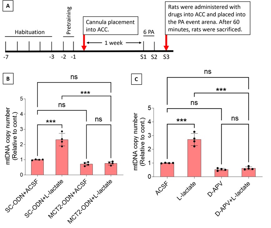
The experiment using AVP to block NMDAR only partially supports the conclusions. Indeed, blocking NMDAR will knock down any response that involves these receptors, whether L-lactate is necessary or not.
In the current study we found that Astrocytic Gi activation in the ACC reduced L-lactate level in the ECF of ACC which was also associated with decreased PGC-1α/SIRT3/ATPB/mtDNA abundance suggesting downregulation of mitochondrial biogenesis pathway. We also found that exogenous administration of L-lactate into the ACC of astrocytic Gi-activated rats rescued this downregulation. In line with this, in a recently published study (Akter et al., 2023), we found upregulation of mitochondrial biogenesis pathway in the hippocampus neurons of exogenous L-lactate-treated anesthetized rats. Another recent study has demonstrated that exercise-induced L-lactate release from skeletal muscle or I.P. injection of L-lactate can induce hippocampal PGC-1α (which is a master regulator of mitochondrial biogenesis) expression and mitochondrial biogenesis in mice (Park et al., 2021). Together, these results provide compelling evidence that L-lactate promotes mitochondrial biogenesis.
L-lactate is known to promote expression of synaptic plasticity genes like Arc, c-Fos, and Zif268 in neurons (Yang et al., 2014). After entry into the neuronal cytoplasm, mainly through MCT2, it is converted into pyruvate by lactate dehydrogenase 1 (LDH1). This conversion also produces NADH, affecting the redox state of the neuron. NADH positively modulates the activity of NMDAR resulting in enhanced Ca2+ currents, the activation of intracellular signaling cascades, and the induction of the expression of plasticity-associated genes (Yang et al., 2014; Magistretti & Allaman, 2018). The study demonstrated that L-lactate–induced plasticity gene expression was abolished in the presence of NMDAR antagonists including D-APV (Yang et al., 2014). These results suggested that the MCT2 and NMDAR are key players in the regulation of L-lactate induced plasticity gene expression.
In the current study, we investigated whether similar mechanisms might be involved in L-lactate-induced neuronal mitochondrial biogenesis. We now used MCT2 antisense oligodeoxynucleotide to decrease the expression of MCT2 (as mentioned in the previous response and Author response image 1B) and showed that MCT2 is necessary for L-lactate-induced mitochondrial biogenesis to manifest, indicating that L-lactate’s entry into the neuron is required. As mentioned before, after entry into neuron, L-lactate is converted into pyruvate by LDH, which also produce NADH, which in turn potentiates NMDAR activity. Therefore, we investigated whether NMDAR activity is required for L-lactate-induced mitochondrial biogenesis. We used D-APV to inhibit NMDAR (Author response image 1C) and found that L-lactate does not increase mtDNA copy number abundance if D-APV is given, suggesting that NMDAR activity is required for L-lactate to promote mitochondrial biogenesis.
NMDAR serves diverse functions. Therefore, as mentioned by the reviewer, blocking NMDAR may knock down many such functions. While our current data only suggests the involvement of MCT2 and NMDAR in the upregulation of mitochondrial biogenesis by L-lactate, we have not investigated other mechanisms and pathways modulating mitochondrial biogenesis that are either dependent or independent of MCT2 and NMDAR activity. Further studies are needed in future to dissect and better understand this interesting observation. We have now clarified this in the discussion section of the manuscript.
Is inhibition of glycogenolysis involved in the observed effects mediated by Gi signaling? Indeed, L-lactate is formed both by glycolysis and glycogenolysis. The authors could test whether the glycogen metabolism-inhibiting drug DAB would mimic the effects of Gi activation.
In this study we have shown that astrocytic Gi activation in the ACC leads to a decrease in the cAMP and L-lactate. L-lactate is produced by glycogenolysis and glycolysis. cAMP in astrocytes acts as a trigger for L-lactate production (Choi et al., 2012; Horvat, Muhič, et al., 2021; Horvat, Zorec, et al., 2021; Zhou et al., 2021) by promoting glycogenolysis and glycolysis (Vardjan et al., 2018; Horvat, Muhič, et al., 2021; Horvat, Zorec, et al., 2021). Therefore, one promising explanation of reduced L-lactate level observed in our study is the reduction of L-lactate production in the astrocyte due to decreased glycogen metabolism as a result of decreased cAMP. We have now mentioned this in the discussion.
DAB is an inhibitor of glycogen phosphorylase that suppresses L-lactate production. It was shown to impair memory by decreasing L-lactate (Newman et al., 2011; Suzuki et al., 2011; Iqbal et al., 2023). As we found that the impairment in the schema memory and mitochondrial biogenesis was associated with decreased L-lactate level in the ACC and that the exogenous L-lactate administration can rescue the impairments, it is likely that DAB will mimic the effect of Gi activation in terms of schema memory and mitochondrial biogenesis. However, further study is needed to confirm this.
Reviewer #2 (Public Review):
The manuscript of Akter et al is an important study that investigates the role of astrocytic Gi signaling in the anterior cingulate cortex in the modulation of extracellular L-lactate level and consequently impairment in flavor-place associates (PA) learning. However, whereas some of the behavioral observations and signaling mechanism data are compelling, the conclusions about the effect on memory are inadequate as they rely on an experimental design that does not allow to differentiate acute or learning effect from the effect outlasting pharmacological treatments, i.e. effect on memory retention. With the addition of a few experiments, this paper would be of interest to the larger group of researchers interested in neuron-glia interactions during complex behavior.
• Largely, I agree with the authors' conclusion that activating Gi signaling in astrocytes impairs PA learning, however, the effect on memory retrieval is not that obvious. All behavioral and molecular signaling effects described in this study are obtained with the continuous presence of CNO, therefore it is not possible to exclude the acute effect of Gi pathway activation in astrocytes. What will happen with memory on retrieval test when CNO is omitted selectively during early, middle, or late session blocks of PA learning?
We have now added 8 more rats to the hM4Di-CNO group (i.e., the group with astrocytic Gi activation) to clarify the memory retrieval. These rats underwent flavor-place paired associate (PA) training similar to the previously described rats (n=7) of this group, that is they received CNO 30 minutes before and 30 minutes after the PA training sessions (S1-2, S4-8, S10-17). However, contrasting to the previous rats of this group which received CNO before PTs (PT1, PT2, PT3), we omitted the CNO (instead administered I.P. saline) selectively on these PTs conducted at the early, middle, and late stage of PA training, as suggested by the reviewer. These newly added rats did not show memory retrieval in these PTs, suggesting that the rats were not learning the PAs from the PA training sessions. See Author response image 2C-E, where this subgroup is denoted as hM4Di-CNO (Saline).
We then continued more PA training sessions (S21 onwards, Author response image 2B) for these rats without CNO. They gradually learned the PAs. PTs (PT5, PT6, PT7; Author response image 2G-I) were done during this continuation phase of PA training; once without CNO (i.e., with I.P. saline instead), and another one with CNO. As seen in the Author response image 2H and 2I, they retrieved the memory when PT6 and PT7 were done without CNO. However, if these PTs were done with CNO, they could not retrieve the memory. Together these results suggest that ACC astrocytic Gi activation by CNO during PT can impair memory retrieval in rats which have already learned the PAs.
As shown in the Author response image 2B, we replaced two original PAs with two new PAs (NPA 9 and 10) at S34. This was followed by PT8 (S35). As seen in Author response image 2J, these rats retrieved the NPA memory if the PT is done without CNO. However, they could not retrieve the NPA memory if the PT was done with CNO. This result suggests that ACC astrocytic Gi activation by CNO during PT can impair NPA memory retrieval.
In summary, these data show that astrocytic Gi activation in the ACC can impair PA memory retrieval. We have integrated this new data and results in the revised manuscript.
Author response image 2.
A. PI (mean ± SD) during the acquisition of the six original PAs (OPAs) (S1-2, 4-8, 10-17) and new PAs (NPAs) (S19) of the control (n=8), hM4Di-CNO (n=15), and rescue (hM4Di-CNO+L-lactate) (n=7) groups. From S6 onwards, hM4Di-CNO group consistently showed lower PI compared to control. However, concurrent L-lactate administration into the ACC (rescue group) can rescue this impairment. B. PI (mean ± SD) of hM4Di-CNO group (n=8) from S21 onwards showing gradual increase in PI when CNO was withdrawn. C, D, and E. Non-rewarded PTs (PT1, PT2, and PT3 conducted on S3, S9, and S18, respectively) to test memory retrieval of OPAs for the control, hM4Di-CNO, and rescue groups. The percentage of digging time at the cued location relative to that at the non-cued locations are shown (mean ± SD). In both PT2 and PT3, the control group spent significantly more time digging the cued sand well above the chance level, indicating that the rats learned OPAs and could retrieve it. Contrasting to this, hM4Di-CNO group did not spend more time digging the cued sand well above the chance level irrespective of CNO administration before the PTs. The rescue group showed results similar to the hM4Di-CNO group if CNO is given without L-lactate. On the other hand, they showed results similar to the control group if L-lactate is concurrently given with CNO, indicating that this group learned OPAs and could retrieve it. p < 0.05, p < 0.01, p < 0.001, one-sample t-test comparing the proportion of digging time at the cued sand well with the chance level of 16.67%. F. Non-rewarded PT4 (S20) which was conducted after replacing two OPAs with two NPAs (NPA 7 & 8) in S19 for the control, hM4Di-CNO, and rescue groups. Results show that the control group spent significantly more time digging the new cued sand well above the chance level indicating that the rats learned the NPAs from S19 and could retrieve it in this PT. Contrasting to this, hM4Di-CNO group did not spend more time digging the new-cued sand well above the chance level irrespective of CNO administration before the PT. The rescue group showed results similar to the hM4Di-CNO group if CNO is given without L-lactate. On the other hand, they showed results similar to the control group if L-lactate is concurrently given with CNO indicating that this group learned NPAs from S19 and could retrieve it. p < 0.001, one-sample t-test comparing the proportion of digging time at the new cued sand well with the chance level of 16.67%. G, H, and I. Non-rewarded PTs (PT5, PT6, and PT7 conducted on S23, S27, and S33, respectively) to test memory retrieval of OPAs for the hM4Di-CNO group. In both PT6 and PT7, the rats spent significantly more time digging the cued sand well above the chance level if the tests are done without CNO, indicating that the rats learned the OPAs and could retrieve it. However, CNO prevented memory retrieval during these PTs. p < 0.001, one-sample t-test comparing the proportion of digging time at the cued sand well with the chance level of 16.67%. J. Non-rewarded PT4 (S35) which was conducted after replacing two OPAs with two NPAs (NPA 9 & 10) in S34 for the hM4Di-CNO group. Results show that the rats spent significantly more time digging the new cued sand well above the chance level if CNO was not given before the PT, indicating that the rats learned the NPAs from S34 and could retrieve it in this PT. However, if CNO is given before the PT, the retrieval is impaired. *p < 0.001, one-sample t-test comparing the proportion of digging time at the new cued sand well with the chance level of 16.67%.
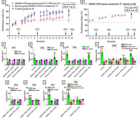
• I found it truly exciting that the administration of exogenous L-lactate is capable to rescue CNO-induced PA learning impairment, when co-applied. Would it be possible that this treatment has a sensitivity to a particular stage of learning (acquisition, consolidation, or memory retrieval) when L-lactate administration would be the most efficacious?
The hM4Di-CNO group, when continued with PA training without CNO (S21-S32) (Author response image 2B), was able to learn the six original PAs (OPAs). In the PT7 done at S33 (Author response image 2I), this group of rats was able to retrieve the memory if the test was done without CNO but could not retrieve the memory if CNO was given. Similarly, the Rescue group (hM4Di-CNO+L-lactate) (Author response image 2A), which received both CNO and L-lactate during PA training sessions (S1-S17), they were able to learn the OPAs. And at PT3 done at S18 (Author response image 2E), these rats were able to retrieve the memory when the test was done with CNO+L-lactate but not if the test is done with only CNO. Together, these results clearly show that ACC astrocytic Gi activation with CNO impairs memory retrieval and exogenous L-lactate can rescue the impairment. Therefore, it can be concluded that the memory retrieval is sensitive to L-lactate.
The PA learning is hippocampus-dependent. Over the course of repeated PA training, systems consolidation occurs in the ACC, after which the already learned PA memory (schema) becomes hippocampus-independent (Tse et al., 2007; Tse et al., 2011). A higher activation (indicated by expression of c-Fos) in the hippocampus relative to the ACC during the early period of schema development, and the reverse at the late stage was observed in our previous study (Liu et al., 2022). However, rapid assimilation of new PA into the ACC requires simultaneous activation/retrieval of previous schema from ACC and hippocampus dependent new PA learning (Tse et al., 2007; Tse et al., 2011). During new PA learning, increase of c-Fos neurons in both CA1 and ACC was detected (Liu et al., 2022).
Our hM4Di-CNO group received CNO 30 mins before and after each PA training session in S1-S17 (Author response image 2A). Also, the Rescue group similarly received CNO+L-lactate before and after each PA training session in S1-S17. Therefore, while this study design allowed us to conclude that ACC astrocytic Gi activation impairs PA learning and that exogenous L-lactate can rescue the impairment, it does not allow clear differentiation of the effects of these treatments on memory acquisition and consolidation. Further studies are needed to investigate this.
• The hypothesis that observed learning impairments could be associated with diminished mitochondrial biogenesis caused by decreased l-lactate in the result of astrocytic Gi-DREADDS stimulation is very appealing, but a few key pieces of evidence are missing. So far, the hypothesis is supported by experiments demonstrating reduced expression of several components of mitochondrial membrane ATP synthase and a decrease in relative mtDNA copy numbers in ACC of rats injected with Gi-DREADDs. L-lactate injections into ACC restored and even further increased the expression of the above-mentioned markers. Co-administration of NMDAR antagonist D-APV or MCT-2 (mostly neuronal) blocker 4-CIN with L-lactate, prevented L-lactate-induced increase in relative mtDNA copy. I am wondering how the interference with mitochondrial biogenesis is affecting neuronal physiology and if it would result in impaired PA learning or schema memory.
The observation of diminished mitochondrial biogenesis in the astrocytic Gi-activated rats that showed impaired PA learning is exciting. However, our study does not provide experimental data on how mitochondrial biogenesis could be associated with impaired PA learning and schema memory. Results from several previous studies linked mitochondrial biogenesis and its regulators such as PGC-1α and SIRT3 to diverse neuronal and cognitive functions as described in the discussion section of the manuscript. In the revised manuscript, we have provided further discussion as follows to discuss potential mechanisms:
“In this study, we have demonstrated that ACC astrocytic Gi activation impairs PA learning and schema formation, PA memory retrieval, and NPA learning and retrieval by decreasing L-lactate level in the ACC. Although we have shown that these impairments are associated with diminished expression of proteins of mitochondrial biogenesis, the precise mechanisms of how astrocytic Gi activation affects neuronal functions and schema memory remain to be elucidated. We previously demonstrated that neuronal inhibition in either the hippocampus or the ACC impairs PA learning and schema formation (Hasan et al., 2019). In another recent study (Liu et al., 2022), we showed that astrocytic Gi activation in the CA1 impaired PA training-associated CA1-ACC projecting neuronal activation. Yao et al. recently showed that reduction of astrocytic lactate dehydrogenase A (an enzyme that reversibly catalyze L-lactate production from pyruvate) in the dorsomedial prefrontal cortex reduces L-lactate levels and neuronal firing frequencies, promoting depressive-like behaviors in mice (Yao et al., 2023). These impairments could be rescued by L-lactate infusion. It is possible that the impairment in PA learning and schema observed in our study might have involved a similar functional consequence of reduced neuronal activity in the ACC neurons upon astrocytic Gi activation.
Schema consolidation is associated with synaptic plasticity-related gene expression (such as Zif268, Arc) in the ACC (Tse et al., 2011). L-lactate, after entry into neurons, can be converted to pyruvate during which NADH is also produced, promoting synaptic plasticity-related gene expression by potentiating NMDA signaling in neurons (Yang et al., 2014; Margineanu et al., 2018). Furthermore, L-lactate acts as an energy substrate to fuel learning-induced de novo neuronal translation critical for long-term memory (Descalzi et al., 2019). On the other hand, mitochondria play crucial role in fueling local translation during synaptic plasticity (Rangaraju et al., 2019). Therefore, it could be hypothesized that the rescue of astrocytic Gi activation-mediated impairment of schema by exogenous L-lactate could have been mediated by facilitating synaptic plasticity-related gene expression by directly fueling the protein translation, potentiating NMDA signaling, as well as increasing mitochondrial capacity for ATP production by promoting mitochondrial biogenesis. Furthermore, the potential involvement of HCAR1, a receptor for L-lactate that may regulate neuronal activity (Bozzo et al., 2013; Tang et al., 2014; Herrera-López & Galván, 2018; Abrantes et al., 2019), cannot be excluded. Future research could explore these potential mechanisms, examining the interactions among them, and determining their relative contributions to schema. Our previous study also showed that ACC myelination is necessary for PA learning and schema formation, and that repeated PA training is associated with oligodendrogenesis in the ACC (Hasan et al., 2019). Oligodendrocytes facilitate fast, synchronized, and energy efficient transfer of information by wrapping axons in myelin sheath. Furthermore, they supply axons with glycolysis products, such as L-lactate, to offer metabolic support (Fünfschilling et al., 2012; Lee et al., 2012). The association of oligodendrogenesis and myelination with schema memory may suggest an adaptive response of oligodendrocytes to enhance metabolic support and neuronal energy efficiency during PA learning. Given the impairments in PA learning observed in the ACC astrocytic Gi-activated rats in the current study, it is reasonable to conclude that the direct metabolic support to axons provided by oligodendrocytes is not sufficient to rescue the schema impairments caused by decreased L-lactate levels upon astrocytic Gi activation. On the other hand, L-lactate was shown to be important for oligodendrogenesis and myelination (Sánchez-Abarca et al., 2001; Rinholm et al., 2011; Ichihara et al., 2017). Therefore, it is tempting to speculate that a decrease in L-lactate level may also impede oligodendrogenesis and myelination, consequently preventing the enhanced axonal support provided by oligodendrocytes and myelin during schema learning. Recently, a study has demonstrated that upon demyelination, mitochondria move from the neuronal cell body to the demyelinated axon (Licht-Mayer et al., 2020). Enhancement of this axonal response of mitochondria to demyelination, by targeting mitochondrial biogenesis and mitochondrial transport from the cell body to axon, protects acutely demyelinated axons from degeneration. Given the connection between schema and increased myelination, it remains an open question whether L-lactate-induced mitochondrial biogenesis plays a beneficial role in schema through a similar mechanism. Nevertheless, our results contribute to the mounting evidence of the glial role in cognitive functions and underscores the new paradigm in which glial cells are considered as integral players in cognitive functions alongside neurons. Disruption of neurons, myelin, or astrocytes in the ACC can disrupt PA learning and schema memory.”
Reviewer #3 (Public Review):
Akter et al. investigated how the astroglial Gi signaling pathway in the rat anterior cingulate cortex (ACC) affects cognitive functions, in particular schema memory formation. Using a stereotactic approach they intracranially introduced AAV8 vectors carrying mCherry-tagged hM4Di DREADD (Designer Receptor Exclusively Activated by Designer Drugs) under astrocyte selective GFAP promotor (AAV8-GFAP-hM4Di-mCherry) into the AAC region of the rat brain. hM4Di DREADD is a genetically modified form of the human M4 muscarinic (hM4) receptor insensitive to endogenous acetylcholine but is activated by the inert clozapine metabolite clozapine-N-oxide (CNO), triggering the Gi signaling pathway. The authors confirmed that hM4Di DREADD is selectively expressed in astrocytes after the application of the AAV8 vector by analysing the mCherry signals and immunolabeling of astrocytes and neurons in the ACC region of the rat brain. They activated hM4Di DREADD (Gi signalling) in astrocytes by intraperitoneal administration of CNO and measured cognitive functions in animals after CNO administration. Activation of Gi signaling in astrocytes by CNO application decreased paired-associate (PA) learning, schema formation, and memory retrieval in tested animals. This was associated with a decrease in cAMP in astrocytes and L-lactate in extracellular fluid as measured by immunohistochemistry in situ and in awake rats by microdialysis, respectively. Administration of exogenous L-lactate rescued the astroglial Gi-mediated deficits in PA learning, memory retrieval, and schema formation, suggesting that activation of astroglial Gi signalling downregulates L-lactate production in astrocytes and its transport to neurons affecting memory formation. Authors also show that expression level of proteins involved in mitochondrial biogenesis, which is associated with cognitive functions, is decreased in neurons, when Gi signalling is activated in astrocytes, and rescued when exogenous L-lactate is applied, suggesting the implication of astrocyte-derived L-lactate in the maintenance of mitochondrial biogenesis in neurons. The latter depended on lactate MCT2 transporter activity and glutamate NMDA receptor activity.
The paper is very well written and discussed. The conclusions of this paper are well supported by the data. Although this is a study that uses established and previously published methodologies, it provides new insights into L-lactate signalling in the brain, particularly in AAC, and further confirms the role of astroglial L-lactate in learning and memory formation. It also raises new questions about the molecular mechanisms underlying astrocyte-derived L-lactate-mediated mitochondrial biogenesis in neurons and its contribution to schema memory formation.
• The authors discuss astrocytic L-lactate signalling without considering the recently discovered L-lactate-sensitive Gs and Gi protein-coupled receptors in the brain, which are present in both astrocytes and neurons. The use of nonendogenous L-lactate receptor agonists (Compound 2, 3-chloro-5-hydroxybenzoic acid) would clarify the implication of L-lactate receptor signalling in schema memory formation.
In the revised manuscript, we have included this point in the discussion section to mention the potential role of HCAR1 in schema memory as follows:
“Schema consolidation is associated with synaptic plasticity-related gene expression (such as Zif268, Arc) in the ACC (Tse et al., 2011). L-lactate, after entry into neurons, can be converted to pyruvate during which NADH is also produced, promoting synaptic plasticity-related gene expression by potentiating NMDA signaling in neurons (Yang et al., 2014; Margineanu et al., 2018). Furthermore, L-lactate acts as an energy substrate to fuel learning-induced de novo neuronal translation critical for long-term memory (Descalzi et al., 2019). On the other hand, mitochondria play crucial role in fueling local translation during synaptic plasticity (Rangaraju et al., 2019). Therefore, it could be hypothesized that the rescue of astrocytic Gi activation-mediated impairment of schema by exogenous L-lactate could have been mediated by facilitating synaptic plasticity-related gene expression by directly fueling the protein translation, potentiating NMDA signaling, as well as increasing mitochondrial capacity for ATP production by promoting mitochondrial biogenesis. Furthermore, the potential involvement of HCAR1, a receptor for L-lactate that may regulate neuronal activity (Bozzo et al., 2013; Tang et al., 2014; Herrera-López & Galván, 2018; Abrantes et al., 2019), cannot be excluded. Future research could explore these potential mechanisms, examining the interactions among them, and determining their relative contributions to schema.”
• The use of control animals transduced with an "empty" AAV9 vector (AAV8-GFAP-mCherry) compared with animals transduced with AAV8-GFAP-hM4Di-mCherry throughout the study would strengthen the results of this study, since transfection itself, as well as overexpression of the mCherry protein, may affect cell function.
We thank the reviewer for pointing this. The schema experiment includes a control group (Control-CNO group) of rats injected with AAV8-GFAP-mCherry bilaterally into the ACC. As shown in Author response image 3, after habituation and pretraining, these rats were trained for PA learning similarly to the other groups. Before 30 mins and after 30 mins of each PA training session, they received I.P. CNO. The PA learning, schema formation, memory retrieval, NPA learning and retrieval, and latency (time needed to commence digging at the correct well) were similar to the control group of rats. This result is consistent with our previous study where rats bilaterally injected with AAV8-GFAP-mCherry into CA1 of hippocampus did not show impairments in PA learning and schema formation upon CNO treatment (Liu et al., 2022).
Author response image 3.
A. PI (mean ± SD) during the acquisition of the original six PAs (OPAs) (S1-2, 4-8, 10-17) and new PAs (NPAs) (S19) of the control (n=6) and control-CNO (n=4) groups. B. Non-rewarded PTs (PT1, PT2, and PT3 done on S3, S9, and S18, respectively) to test memory retrieval of OPAs for the control-CNO group. C. Non-rewarded PT4 (S20) which was done after replacing two OPAs with two NPAs (NPA 7 & 8) in S19 for the control-CNO group. D. Latency (in seconds) before commencing digging at the correct well for control and control-CNO groups. Data shown as mean ± SD.
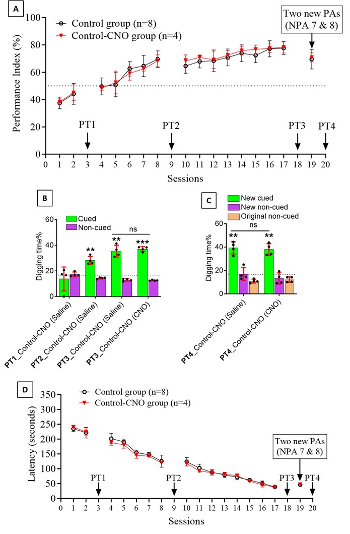
References
Abrantes, H. d. C., Briquet, M., Schmuziger, C., Restivo, L., Puyal, J., Rosenberg, N., Rocher, A.-B., Offermanns, S., & Chatton, J.-Y. (2019). The Lactate Receptor HCAR1 Modulates Neuronal Network Activity through the Activation of Gα and Gβγ Subunits. The Journal of Neuroscience, 39(23), 4422-4433. https://doi.org/10.1523/jneurosci.2092-18.2019
Akter, M., Ma, H., Hasan, M., Karim, A., Zhu, X., Zhang, L., & Li, Y. (2023). Exogenous L-lactate administration in rat hippocampus increases expression of key regulators of mitochondrial biogenesis and antioxidant defense [Original Research]. Frontiers in Molecular Neuroscience, 16. https://doi.org/10.3389/fnmol.2023.1117146
Bozzo, L., Puyal, J., & Chatton, J.-Y. (2013). Lactate Modulates the Activity of Primary Cortical Neurons through a Receptor-Mediated Pathway. PLoS One, 8(8), e71721. https://doi.org/10.1371/journal.pone.0071721
Choi, H. B., Gordon, G. R., Zhou, N., Tai, C., Rungta, R. L., Martinez, J., Milner, T. A., Ryu, J. K., McLarnon, J. G., Tresguerres, M., Levin, L. R., Buck, J., & MacVicar, B. A. (2012). Metabolic communication between astrocytes and neurons via bicarbonate-responsive soluble adenylyl cyclase. Neuron, 75(6), 1094-1104. https://doi.org/10.1016/j.neuron.2012.08.032
Covelo, A., Eraso-Pichot, A., Fernández-Moncada, I., Serrat, R., & Marsicano, G. (2021). CB1R-dependent regulation of astrocyte physiology and astrocyte-neuron interactions. Neuropharmacology, 195, 108678. https://doi.org/https://doi.org/10.1016/j.neuropharm.2021.108678
Descalzi, G., Gao, V., Steinman, M. Q., Suzuki, A., & Alberini, C. M. (2019). Lactate from astrocytes fuels learning-induced mRNA translation in excitatory and inhibitory neurons. Communications Biology, 2(1), 247. https://doi.org/10.1038/s42003-019-0495-2
Endo, F., Kasai, A., Soto, J. S., Yu, X., Qu, Z., Hashimoto, H., Gradinaru, V., Kawaguchi, R., & Khakh, B. S. (2022). Molecular basis of astrocyte diversity and morphology across the CNS in health and disease. Science, 378(6619), eadc9020. https://doi.org/10.1126/science.adc9020
Fünfschilling, U., Supplie, L. M., Mahad, D., Boretius, S., Saab, A. S., Edgar, J., Brinkmann, B. G., Kassmann, C. M., Tzvetanova, I. D., Möbius, W., Diaz, F., Meijer, D., Suter, U., Hamprecht, B., Sereda, M. W., Moraes, C. T., Frahm, J., Goebbels, S., & Nave, K.-A. (2012). Glycolytic oligodendrocytes maintain myelin and long-term axonal integrity. Nature, 485(7399), 517-521. https://doi.org/10.1038/nature11007
Harris, R. A., Lone, A., Lim, H., Martinez, F., Frame, A. K., Scholl, T. J., & Cumming, R. C. (2019). Aerobic Glycolysis Is Required for Spatial Memory Acquisition But Not Memory Retrieval in Mice. eNeuro, 6(1). https://doi.org/10.1523/ENEURO.0389-18.2019
Hasan, M., Kanna, M. S., Jun, W., Ramkrishnan, A. S., Iqbal, Z., Lee, Y., & Li, Y. (2019). Schema-like learning and memory consolidation acting through myelination. FASEB J, 33(11), 11758-11775. https://doi.org/10.1096/fj.201900910R
Herrera-López, G., & Galván, E. J. (2018). Modulation of hippocampal excitability via the hydroxycarboxylic acid receptor 1. Hippocampus, 28(8), 557-567. https://doi.org/https://doi.org/10.1002/hipo.22958
Horvat, A., Muhič, M., Smolič, T., Begić, E., Zorec, R., Kreft, M., & Vardjan, N. (2021). Ca2+ as the prime trigger of aerobic glycolysis in astrocytes. Cell Calcium, 95, 102368. https://doi.org/https://doi.org/10.1016/j.ceca.2021.102368
Horvat, A., Zorec, R., & Vardjan, N. (2021). Lactate as an Astroglial Signal Augmenting Aerobic Glycolysis and Lipid Metabolism [Review]. Frontiers in Physiology, 12. https://doi.org/10.3389/fphys.2021.735532
Ichihara, Y., Doi, T., Ryu, Y., Nagao, M., Sawada, Y., & Ogata, T. (2017). Oligodendrocyte Progenitor Cells Directly Utilize Lactate for Promoting Cell Cycling and Differentiation. J Cell Physiol, 232(5), 986-995. https://doi.org/10.1002/jcp.25690
Iqbal, Z., Liu, S., Lei, Z., Ramkrishnan, A. S., Akter, M., & Li, Y. (2023). Astrocyte L-Lactate Signaling in the ACC Regulates Visceral Pain Aversive Memory in Rats. Cells, 12(1), 26. https://www.mdpi.com/2073-4409/12/1/26
Jourdain, P., Rothenfusser, K., Ben-Adiba, C., Allaman, I., Marquet, P., & Magistretti, P. J. (2018). Dual action of L-Lactate on the activity of NR2B-containing NMDA receptors: from potentiation to neuroprotection. Sci Rep, 8(1), 13472. https://doi.org/10.1038/s41598-018-31534-y
Kofuji, P., & Araque, A. (2021). G-Protein-Coupled Receptors in Astrocyte-Neuron Communication. Neuroscience, 456, 71-84. https://doi.org/10.1016/j.neuroscience.2020.03.025
Lee, Y., Morrison, B. M., Li, Y., Lengacher, S., Farah, M. H., Hoffman, P. N., Liu, Y., Tsingalia, A., Jin, L., Zhang, P. W., Pellerin, L., Magistretti, P. J., & Rothstein, J. D. (2012). Oligodendroglia metabolically support axons and contribute to neurodegeneration. Nature, 487(7408), 443-448. https://doi.org/10.1038/nature11314
Licht-Mayer, S., Campbell, G. R., Canizares, M., Mehta, A. R., Gane, A. B., McGill, K., Ghosh, A., Fullerton, A., Menezes, N., Dean, J., Dunham, J., Al-Azki, S., Pryce, G., Zandee, S., Zhao, C., Kipp, M., Smith, K. J., Baker, D., Altmann, D., Anderton, S. M., Kap, Y. S., Laman, J. D., Hart, B. A. t., Rodriguez, M., Watzlawick, R., Schwab, J. M., Carter, R., Morton, N., Zagnoni, M., Franklin, R. J. M., Mitchell, R., Fleetwood-Walker, S., Lyons, D. A., Chandran, S., Lassmann, H., Trapp, B. D., & Mahad, D. J. (2020). Enhanced axonal response of mitochondria to demyelination offers neuroprotection: implications for multiple sclerosis. Acta Neuropathologica, 140(2), 143-167. https://doi.org/10.1007/s00401-020-02179-x
Liu, S., Wong, H. Y., Xie, L., Iqbal, Z., Lei, Z., Fu, Z., Lam, Y. Y., Ramkrishnan, A. S., & Li, Y. (2022). Astrocytes in CA1 modulate schema establishment in the hippocampal-cortical neuron network. BMC Biol, 20(1), 250. https://doi.org/10.1186/s12915-022-01445-6
Magistretti, P. J., & Allaman, I. (2018). Lactate in the brain: from metabolic end-product to signalling molecule. Nat Rev Neurosci, 19(4), 235-249. https://doi.org/10.1038/nrn.2018.19
Margineanu, M. B., Mahmood, H., Fiumelli, H., & Magistretti, P. J. (2018). L-Lactate Regulates the Expression of Synaptic Plasticity and Neuroprotection Genes in Cortical Neurons: A Transcriptome Analysis. Front Mol Neurosci, 11, 375. https://doi.org/10.3389/fnmol.2018.00375
Netzahualcoyotzi, C., & Pellerin, L. (2020). Neuronal and astroglial monocarboxylate transporters play key but distinct roles in hippocampus-dependent learning and memory formation. Progress in Neurobiology, 194, 101888. https://doi.org/https://doi.org/10.1016/j.pneurobio.2020.101888
Newman, L. A., Korol, D. L., & Gold, P. E. (2011). Lactate produced by glycogenolysis in astrocytes regulates memory processing. PLoS One, 6(12), e28427. https://doi.org/10.1371/journal.pone.0028427
Park, J., Kim, J., & Mikami, T. (2021). Exercise-Induced Lactate Release Mediates Mitochondrial Biogenesis in the Hippocampus of Mice via Monocarboxylate Transporters. Front Physiol, 12, 736905. https://doi.org/10.3389/fphys.2021.736905
Peterson, S. M., Pack, T. F., & Caron, M. G. (2015). Receptor, Ligand and Transducer Contributions to Dopamine D2 Receptor Functional Selectivity. PLoS One, 10(10), e0141637. https://doi.org/10.1371/journal.pone.0141637
Rangaraju, V., Lauterbach, M., & Schuman, E. M. (2019). Spatially Stable Mitochondrial Compartments Fuel Local Translation during Plasticity. Cell, 176(1), 73-84.e15. https://doi.org/10.1016/j.cell.2018.12.013
Rinholm, J. E., Hamilton, N. B., Kessaris, N., Richardson, W. D., Bergersen, L. H., & Attwell, D. (2011). Regulation of oligodendrocyte development and myelination by glucose and lactate. J Neurosci, 31(2), 538-548. https://doi.org/10.1523/JNEUROSCI.3516-10.2011
Sánchez-Abarca, L. I., Tabernero, A., & Medina, J. M. (2001). Oligodendrocytes use lactate as a source of energy and as a precursor of lipids. Glia, 36(3), 321-329. https://doi.org/10.1002/glia.1119
Suzuki, A., Stern, S. A., Bozdagi, O., Huntley, G. W., Walker, R. H., Magistretti, P. J., & Alberini, C. M. (2011). Astrocyte-neuron lactate transport is required for long-term memory formation. Cell, 144(5), 810-823.
Tang, F., Lane, S., Korsak, A., Paton, J. F. R., Gourine, A. V., Kasparov, S., & Teschemacher, A. G. (2014). Lactate-mediated glia-neuronal signalling in the mammalian brain. Nature Communications, 5(1), 3284. https://doi.org/10.1038/ncomms4284
Tauffenberger, A., Fiumelli, H., Almustafa, S., & Magistretti, P. J. (2019). Lactate and pyruvate promote oxidative stress resistance through hormetic ROS signaling. Cell Death Dis, 10(9), 653. https://doi.org/10.1038/s41419-019-1877-6
Tse, D., Langston, R. F., Kakeyama, M., Bethus, I., Spooner, P. A., Wood, E. R., Witter, M. P., & Morris, R. G. (2007). Schemas and memory consolidation. Science, 316(5821), 76-82. https://doi.org/10.1126/science.1135935
Tse, D., Takeuchi, T., Kakeyama, M., Kajii, Y., Okuno, H., Tohyama, C., Bito, H., & Morris, R. G. (2011). Schema-dependent gene activation and memory encoding in neocortex. Science, 333(6044), 891-895. https://doi.org/10.1126/science.1205274
Vardjan, N., Chowdhury, H. H., Horvat, A., Velebit, J., Malnar, M., Muhič, M., Kreft, M., Krivec, Š. G., Bobnar, S. T., Miš, K., Pirkmajer, S., Offermanns, S., Henriksen, G., Storm-Mathisen, J., Bergersen, L. H., & Zorec, R. (2018). Enhancement of Astroglial Aerobic Glycolysis by Extracellular Lactate-Mediated Increase in cAMP [Original Research]. Frontiers in Molecular Neuroscience, 11. https://doi.org/10.3389/fnmol.2018.00148
Vezzoli, E., Cali, C., De Roo, M., Ponzoni, L., Sogne, E., Gagnon, N., Francolini, M., Braida, D., Sala, M., Muller, D., Falqui, A., & Magistretti, P. J. (2020). Ultrastructural Evidence for a Role of Astrocytes and Glycogen-Derived Lactate in Learning-Dependent Synaptic Stabilization. Cereb Cortex, 30(4), 2114-2127. https://doi.org/10.1093/cercor/bhz226
Wang, J., Tu, J., Cao, B., Mu, L., Yang, X., Cong, M., Ramkrishnan, A. S., Chan, R. H. M., Wang, L., & Li, Y. (2017). Astrocytic l-Lactate Signaling Facilitates Amygdala-Anterior Cingulate Cortex Synchrony and Decision Making in Rats. Cell Rep, 21(9), 2407-2418. https://doi.org/10.1016/j.celrep.2017.11.012
Yang, J., Ruchti, E., Petit, J. M., Jourdain, P., Grenningloh, G., Allaman, I., & Magistretti, P. J. (2014). Lactate promotes plasticity gene expression by potentiating NMDA signaling in neurons. Proc Natl Acad Sci U S A, 111(33), 12228-12233. https://doi.org/10.1073/pnas.1322912111
Yao, S., Xu, M.-D., Wang, Y., Zhao, S.-T., Wang, J., Chen, G.-F., Chen, W.-B., Liu, J., Huang, G.-B., Sun, W.-J., Zhang, Y.-Y., Hou, H.-L., Li, L., & Sun, X.-D. (2023). Astrocytic lactate dehydrogenase A regulates neuronal excitability and depressive-like behaviors through lactate homeostasis in mice. Nature Communications, 14(1), 729. https://doi.org/10.1038/s41467-023-36209-5
Yu, X., Zhang, R., Wei, C., Gao, Y., Yu, Y., Wang, L., Jiang, J., Zhang, X., Li, J., & Chen, X. (2021). MCT2 overexpression promotes recovery of cognitive function by increasing mitochondrial biogenesis in a rat model of stroke. Anim Cells Syst (Seoul), 25(2), 93-101. https://doi.org/10.1080/19768354.2021.1915379
Zhou, Z., Okamoto, K., Onodera, J., Hiragi, T., Andoh, M., Ikawa, M., Tanaka, K. F., Ikegaya, Y., & Koyama, R. (2021). Astrocytic cAMP modulates memory via synaptic plasticity. Proc Natl Acad Sci U S A, 118(3), e2016584118. https://doi.org/10.1073/pnas.2016584118
Zhu, J., Hu, Z., Han, X., Wang, D., Jiang, Q., Ding, J., Xiao, M., Wang, C., Lu, M., & Hu, G. (2018). Dopamine D2 receptor restricts astrocytic NLRP3 inflammasome activation via enhancing the interaction of β-arrestin2 and NLRP3. Cell Death Differ, 25(11), 2037-2049. https://doi.org/10.1038/s41418-018-0127-2
Author Response:
Reviewer #1 (Public Review):
The physical principles underlying oligomerization of GPCRs are not well understood. Here, authors focused on oligomerization of A2AR. They found that oligomerization of A2AR is mediated by the intrinsically disordered, extramembraneous C-terminal tail. Using experiment and MD simulation, they mapped the regions that are responsible for oligomerization and dissected the driving forces in oligomerization.
This is a nice piece of work that applies fundamental physical principles to the understanding of an important biological problem. It is a significant finding that oligomerization of A2AR is mediated by multiple weak interactions that are "tunable" by environmental factors. It is also interesting that solute-induced, solvent-mediated "depletion interactions" can be a key driving force in membrane protein-protein interactions.
Although this work is potentially a significant contribution to the fields of GPCRs and molecular biophysics of membrane proteins in general, there are several concerns that would need to be implemented to strengthen the conclusions.
1) How reasonably would the results obtained in the micellar environment be translated into the phenomenon in the cell membranes?
1a) Here authors measured oligomerization of A2AR in detergent micelles, not in the bilayer or cellular context. Although the cell membranes would provide another layer of complexity, the hydrophobic properties and electrostatics of the negatively charged membrane surface may cooperate or compete with the interactions mediated by the C-terminal tail, especially if the oligomerization is mediated by multiple weak interactions.
The translatability of properties of membrane proteins in detergent micelles to the cellular context is a valid concern. However, this shortcoming applies to all biophysical studies of membrane proteins in non-native environments. Even for membrane proteins reconstituted in liposomes, the question arises whether the artificial lipid composition that differs from that in the human plasma membrane would alter protein properties, especially as surface charges and cholesterol content can impact membrane protein dynamics, association, and stability. In that sense, this question cannot be answered satisfyingly, especially for GPCRs that are notoriously difficult to isolate. However, we can offer some perspectives. The propensity for membrane proteins to associate and oligomerize, if anything, is greater in lipid bilayers compared to that in detergent micelles, while detergent micelles can effectively solubilize membrane protein monomers (Popot and Engelman, Biochem 1990, 29 (17), 4031–4037). Hence, the findings that A2AR readily oligomerizes in detergent micelles and that the degree of oligomerization can be systematically tuned by the C-terminal length of A2AR in the same micellar system suggest that inter-A2AR interactions are modulating receptor oligomerization; we speculate that A2AR oligomers will be present or be enhanced in the lipid bilayer environment. In fact, in the cellular context, it has been shown that A2AR assembles into homodimers at the cell surface in transfected HEK293 cells (Canals et al, J Neurochem 2004, 88, 726–734) and into higher- order oligomers at the plasma membrane in Cath.A differentiated neuronal cells (Vidi et al, FEBS Lett 2008, 582, 3985–3990). Furthermore, C-terminally truncated A2AR has been demonstrated to show no protein aggregation or clustering on the cell surface, a process otherwise observed in the WT form (Burgueno et al, J Biol Chem 2003, 278 (39), 37545–37552). These results provide the research community with a valid starting point to discover factors that control oligomerization of A2AR in the cellular context.
1b) Related to the point above (1a), I wonder if MD simulation could provide an insight into the role of the lipid bilayer in the inter- or intra-molecular interactions involving the tail. Although the neutral POPC bilayer was employed in the simulation, the tail-membrane interaction may affect oligomerization since the tail is intrinsically disordered and possess a significant portion of nonpolar residues (Fig. S4).
The reviewer brings up a valid point about the ability for MD simulations to provide insights into the role of membrane-protein interactions. In response to the reviewer, we performed additional analysis focusing on the interactions of the C-terminus with the lipid bilayer. Overall, as the C-terminus is extended, there is a decrease in its interaction with the cytoplasmic leaflet of the membrane (left figure below). More specifically, we find that the C-terminal segment associated with helix 8 (residues 291 to 314) interacts tightly with the membrane, while the rest of the C-terminus (an intrinsically disordered segment) more weakly interacts with the membrane, regardless of truncation (right figure below). As the C-terminus is extended, the inherent conformational flexibility leads to a decrease in the interactions between the protein and the bilayer. We also observe that shorter stretches of the disordered segment do have the ability to interact more closely with the membrane. While these portions include charged residues that can participate in formation of the dimer interface, no general trends are observed. We therefore cannot draw any conclusions regarding the role of C-terminal-membrane interactions on the dimerization of A2AR. What we do know is that the MD simulations presented here should be considered a model study that reveals that the charged and disordered C-terminus of A2AR can account for oligomerization via multiple and weak inter-protomer contacts.
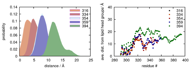
MD simulations showing (Left) average distance of all C-terminal residues and (right) average per-residue distance from the cytoplasmic membrane of the lipid bilayer.
2) Ensuring that the oligomer distributions are thermodynamic products.
Since authors interpret the SEC results on the basis of thermodynamic concepts (driving forces, depletion interactions, etc.), it would be important to verify that the distribution of different oligomeric states is the outcome of the thermodynamic control. There is a possibility that the distribution is the outcome of the "kinetic trapping" during detergent solubilization.
This is an important question. As we have shown in the manuscript, the A2AR dimer level was found to be reduced in the presence of TCEP (Figure 2B), suggesting that disulfide linkages have a role in facilitating A2AR oligomerization. However, disulfide cross-linking reaction cannot be the sole driving force of A2AR oligomerization because (1) a significant population of A2AR dimer remained resistant to TCEP (Figure 2B), (2) A2AR oligomer levels decreased progressively with the shortening of the C-terminus (Figure 3), and (3) A2AR oligomerization is driven by depletion interactions enhanced with increasing ionic strength (Figure 5).
To answer whether A2AR oligomer is a thermodynamic or kinetic product, we tested the stability and reversibility of the A2AR monomer and dimer/oligomer population. We used SEC to separate these populations of both the A2AR-WT and A2AR-Q372ΔC variants, then performed a second round of SEC to observe their repopulation, if any. The results are summarized in the figure below, which we will include in the revised manuscript as Figure 5-figure supplement 1.
We find that the SEC-separated monomers repopulate measurably into dimer/oligomer, with the total oligomer level after redistribution comparable with that of the initial samples for both A2AR WT (initial: 2.87; redistributed: 1.60) and A2AR-Q372ΔC (initial: 1.49; redistributed: 1.40) (Figure 5-figure supplement 1A). This observation indicates that A2AR oligomer is a thermodynamic product with a lower free energy compared with that of the monomer. This is consistent with the results we have shown in the manuscript that the oligomer levels of A2AR-WT are consistent (1.34–2.87; Table S1) and that A2AR oligomerization can be modulated with ionic strengths via depletion interactions (Figure 5).
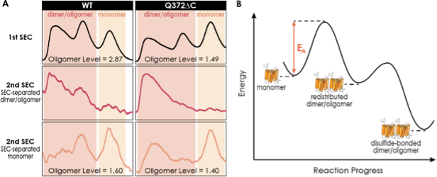
Figure S5. The dimer/oligomerization of A2AR is a thermodynamic process where the dimer and HMW oligomer once formed are kinetically trapped. (A) SEC chromatograms of the consecutive rounds of SEC performed on A2AR-WT and Q372ΔC. The first rounds of SEC are to separate the dimer/oligomer population and the monomer population, while the second rounds of SEC are performed on these SEC-separated populations to assess their stability and reversibility. The total oligomer level is expressed relative to the monomeric population in arbitrary units. (B) Energy diagram depicting A2AR oligomerization progress. The monomer needs to overcome an activation barrier (EA), driven by depletion interactions, to form the dimer/oligomer. Once formed, the dimer/oligomer populations are kinetically trapped by disulfide linkages.
Interestingly, the SEC-separated dimer/oligomer populations do not repopulate to form monomers (Figure 5-figure supplement 1). This observation is, again, consistent with a published study of ours on A2AR dimers (Schonenbach et al, FEBS Lett 2016, 590, 3295–3306). This observation furthermore indicates that once the oligomers are formed, some are kinetically trapped and thus cannot redistribute into monomers.
We believe that disulfide linkages are likely candidates that kinetically stabilize A2AR oligomers, as demonstrated by their redistribution into monomers only in the presence of a reducing agent (Figure 2B). Taken together, we suggest that A2AR oligomerization is a thermodynamic process (Figure 5-figure supplement 1B), with the monomer overcoming the activation energy (EA) by depletion interactions to repopulate into dimer/oligomer with a slightly lower free energy (given that we see a distribution between the two). Once formed, the redistributed dimer/oligomer populations can be kinetically stabilized by disulfide linkages.
3) The claim that the C-terminal tail is engaged in "cooperative" interactions is too qualitative (p. 11 line 274, p.12 line 279 and p.18 line 426).
This claim seems derived from Fig. 3b and Figs. 4b-c. However, the gradual decrease in the dimer level and the number of interactions may indicate that different parts in the C-terminal tail contribute to dimerization additively rather than cooperatively. The large decrease in the number of interactions may stem from the large decrease in the length (395 to 354). Probably, a more quantitative measure would be the number of interactions (H-bonds/salt bridges) normalized to the tail length upon successive truncation. Even in that case, the polar/charged residues would not be uniformly distributed along the primary sequence, making the quantitative argument of cooperativity challenging.
The request to clarify our basis to refer to a cooperative interaction is well taken. Figure 4B and 4C show that the truncation of one part of the C-terminus (segment 335–394) leads to a reduction in contacts of a different part (segment 291–334) of A2AR. Therefore, we conclude that the binding interactions that occur in segment 291–334 are altered by the interactions exerted by the segment 335–394. This characteristic is consistent with allosteric interactions. We believe that characterizing these interactions as “cooperative” is possible but is not fully justified in this work. We also agree with the comment that quantifying the role and segments involved in contacts would be challenging. The manuscript has been amended to use the term “allosteric” in place of “cooperative”.
4) On the compactness and conformation of the C-terminal tail:
Although the C-terminal tail is known as "intrinsically disordered", the results seem to indicate that its conformation is rather compact (or collapsed) with a number of intra- and intermolecular polar interactions (Fig. 4) and buried nonpolar residues (Fig. 6), which are subject to depletion interactions (Fig. 5). This raises a question if the tail indeed "intrinsically disordered" as is known. Recent folding studies on IDPs (Riback et al. Science 2017, 358, 238-; Best, Curr Opin Struct Biol 2020, 60, 27-) suggest that IDPs are partially expanded or expanded rather than collapsed.
We agree that our results seem to suggest that the conformation of the C-terminus could be partially compact. However, by stating that the C-terminus on average is an intrinsically disordered region (IDR), we do not exclude the possibility of partially structured regions, or greater compactness than that of an excluded volume polymer. IDR or IDP should refer to all proteins or protein regions that do not adopt a unique structure. By that standard, we know that the C-terminus of A2AR falls into that category according to our experiments and MD simulation, as well as the literature. In isolation, the majority the C-terminus is indeed an IDR, as has been demonstrated not only by simulations but also by experimental data. In fact, the C-terminus exhibits partial alpha-helical structure, and transiently populates beta-sheet conformations, depending on its state and buffer conditions (Piirainen et al, Biophys J 2015, 108 (4), 903–917). The literature studies suggest that A2AR’s C-terminus may adopt a greater level of compactness when interactions are formed between the C-terminus and the rest of the A2AR oligomer.
Reviewer #2 (Public Review):
The authors expressed A2A receptor as wild type and modified with truncations/mutations at the C-terminus. The receptor was solubilized in detergent solution, purified via a C-terminal deca-His tag and the fraction of ligand binding-competent receptor separated by an affinity column. Receptor oligomerization was studied by size exclusion chromatography on the purified receptor solubilized in a DDM/CHAPS/CHS detergent solution. It was observed that truncation greatly reduces the tendency of A2A to form dimers and oligomers. Mechanistic insights into interactions that facilitate oligomerization were obtained by molecular simulations and the study of aggregation behavior of peptide sequences representing the C-terminus of A2A. It is concluded that a multitude of interactions including disulfide linkages, hydrogen bonds electrostatic- and depletion interactions contribute to aggregation of the receptor.
The general conclusions appear to be correct and the paper is well written. This is a study of protein association in detergent solution. It is conceivable that observations are relevant for A2A receptors in cell membranes as well. However, extrapolation of mechanisms observed on receptor in detergent micelles to receptor in membranes should proceed with caution. In particular, the spatial arrangement of oligomerized receptor molecules in micelles may differ from arrangement in lipid bilayers. The lipid matrix may have a profound influence on oligomerization.
The ultimate question to answer is how oligomerization alters receptor function. This will have to be addressed in a future study.
We could not agree more. We address the concern regarding the translatability of properties of membrane proteins in detergent micelles to the cellular context in our response to Reviewer 1. In short, we believe the general propensity for A2AR to form dimers/oligomers and the role of the C-terminus will hold in the cellular context. However, even if it does not, given that biophysical structure-function studies of GPCRs are conducted in detergent micelles and other artificial environments, it is critical to understand the role of the C-terminus in the oligomerization of reconstituted A2AR in detergent micelles. How oligomerization alters receptor function is a question that is always on our mind and should be the the focus of future studies. Indeed, it has been demonstrated that truncation of the A2AR C-terminus significantly reduces receptor association with Gαs and cAMP production in cellular assays (Koretz et al, Biophys J 2021, https://doi.org/10.1016/j.bpj.2021.02.032). The results presented in this manuscript, which have demonstrated the impact of C-terminal truncation on A2AR oligomerization, will offer critical understanding for such study of the functional consequences of A2AR oligomerization.
Reviewer #3 (Public Review):
The work of Nguyen et al. demonstrates the relevant role of the C-terminus of A2AR for its homo-oligomerization. A previous work (Schonenbach et al. 2016) found that a point mutation of C394 in the C-terminus (C394S) reduces homo-oligomerization. Following this direction, more mutants were generated, the C-terminus was also truncated at different levels, and, using size-exclusion chromatography (SEC), the oligomerization levels of A2AR variants were assessed. Overall, these experiments support the role of the C-terminus in the oligomerization process. MD studies were performed and the non-covalent interactions were monitored. To 'identify the types of non-covalent interaction(s)', A2AR variants were also analysed modulating the ionic strength from 0.15 to 0.95 M. The C-terminus peptides were investigated to assess their interaction in absence of the TM domain.
The SEC results on the A2AR variants strongly support the main conclusion of the paper, but some passages and methodologies are less convincing. The different results obtained for dimerization and oligomerization are low discussed. The MD simulations are performed on models that are not accurately described - structural information currently available may compromise the quality of the model and the validity of the results (i.e., applying MD simulations to low-resolution models may not be appropriate for the goal of this analysis, moreover the formation of disulfide bonds cannot be simulated but this can affect the conformation and consequently the interactions to be monitored). Although the C-terminus is suggested as 'a driving factor for the oligomerization', the TM domain is indeed involved in the process and if and how it will be affected by modulating the solvent ionic strength should be discussed.
We thank the reviewer for the overall positive assessment and critical input. We will respond to the comments as followed.
The qualitative trend for dimerization is consistent with that for oligomerization, as demonstrated in Figs. 2A, 3B, and 5. For example, a reduction in both dimerization and oligomerization was observed upon C394X mutations (Figure 2A), as well as upon systematic truncations (Figure 3B), while very similar trends were seen for the change in the dimer and oligomer levels of all four constructs upon variation of ionic strength (Figure 5).
We agree that the experimental observation and MD simulation only incompletely describe the state of the A2AR dimer/oligomer. For example, we discover the impact of ERR:AAA mutations of the C-terminus (Figure 3C) on oligomer formation, but do not know whether this segment interacts with the TM domain or C-terminus of the neighboring A2AR. MD simulations suggest that the inter-protomer interface certainly involves inter-C-termini contact. We also mention that the A2AR oligomeric interfaces could be asymmetric, suggesting that the C-terminus can interact with other parts of the receptor, including the TM domain. However, we do not have evidence that the TM domain directly interact with each other to stabilize A2AR oligomers, and thus cannot discuss the effect of the solvent ionic strength on how the TM domain contributes to A2AR oligomerization. We minimize such discussion in our manuscript because we have incomplete insights. What we can say is that multiple and weak inter-protomer interactions that contribute to the dimer and oligomer interface formation prominently involve the C-terminus. Ultimately, the structure of the A2AR dimer/oligomer needs to be solved to answer the reviewer’s question fully.
With respect to the validity of our model, we restricted ourselves to using the best-available X-ray crystal structure for A2AR. Since this structure (PDB 5G53) does not include the entire C-terminus, we resorted to using homology modeling software (i.e., MODELLER) to predict the structures of the C-terminus. In our model, the first segment of the C-terminus consisting of residues 291 to 314 were modeled as a helical segment parallel to the cytoplasmic membrane surface while the rest of the C-terminus was modeled as intrinsically disordered. MODELLER is much more accurate in structural predictions for segments less than 20 residues. This limitation necessitated that we run an equilibrium MD simulation for 2 µs to obtain a well-equilibrated structure that possesses a more viable starting conformation. We have included this detailed description of our model in lines 641–650. To validate our models of all potential variants of A2AR, we calculated the RMSD and RMSF for each truncated variant. Our results clearly show that the transmembrane helical bundle is very stable, as expected, and that the C-terminus is more flexible (see figure below). This flexibility is somewhat consistent for lengths up to 359 residues, with a more noticeable increase in flexibility for the 394-residue variant of A2AR.
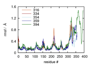
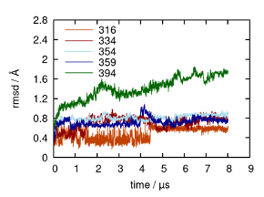
Root mean square fluctuation (RMSF) from sample trajectories of truncated variants modeled from the crystal structure of the adenosine A2AR bound to an engineered G protein (PDB ID 5G53), and the root mean square deviation (RMSD) of the C-terminus of each variant starting from residue 291.
Author Response:
Reviewer #1 (Public Review):
Wang et al., investigated the role of RNA m6A modification in intestinal epithelial cells (IECs) in the context of rotavirus infection. The authors found that the mice which specifically lacks METTL3 in IECs show resistance to rotavirus infection. They attributed this effect to increased IFN and ISG expression presumably via IRF7 upregulation. Further genetic IRF7 ablation in IECs led to the sensitivity rotavirus infection. They also found that ALKBH5 is suppressed by a rotaviral protein, although the knockout of ALKBH5 in IECs did not influence viral infection.
Overall, although the resistance of IEC-specific METTL3-deficient mice upon rotavirus infection via the control of IRF7 is a novel and interesting finding, the proposed model is not fully supported by the findings here. Especially, the following points need to be addressed:
We are grateful to the reviewer for the complimentary summary of our research. We also appreciate the valuable experiments suggested by the reviewer to improve our manuscript. We have added additional important controls and mechanistic data to further support our conclusions.
1) The m6A dot blot used in Figure 1 is not a good measurement system of total m6A modification levels, because the antibody used here also detects other RNA modification, m6Am (PMID: 31676230). Therefore, it is unclear if the increase of m6A dot blot intensity is due to the increase of m6A in RNAs mediated by METTL3 in IECs. The authors should investigate the m6A levels in IECs, not BMDMs, under METTL3 deficiency. Ideally, this analysis should be done using mass spectrometry.
We thank the reviewer for raising a critical point. We have tried several methods to avoid the potential non-specific detection of the previous antibody (Synaptic System, #202003) we used, which was reported to detect m6Am as well.
1.We have included Dot Blot data for m6A modification in Mettl3^△IEC and WT IECs during RV infection by using another m6A antibody (Anti-N6-methyladenosine (m6A), Sigma-Aldrich, Cat. No. ABE572-I). (see below and also Fig. 1d, 1e)
2.We have included mass spectrometry data for m6A modification in IECs during development (see below and also Fig. 1c) or RV infection (see below and also Fig. s3a).
These data suggested m6A modifications in IECs are indeed regulated during the development or RV infection. We have included the descriptions in the text.
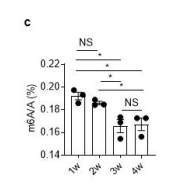
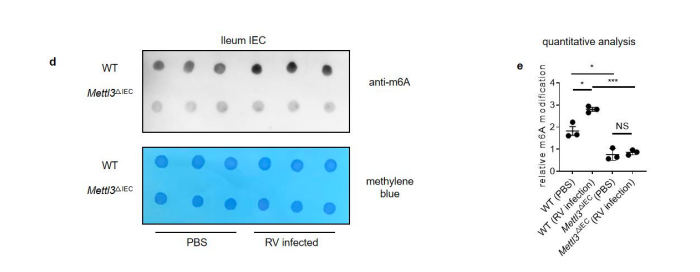
Figure 1. Rotavirus infection increases global m6A modifications, and Mettl3 deficiency in intestinal epithelial cells results in increased resistance to rotavirus infection. (c) MS analysis of m6A level in ileum tissue from mice with different ages. (mean ± SEM), Statistical significance was determined by Student’s t-test (*P < 0.05, NS., not significant). (d) WT and Mettl3^△IEC mice were infected by rotavirus EW strain at 8 days post birth. m6A dot blot analysis of total RNA in ileum IEC at 2 dpi. Methylene blue (MB) staining was the loading control. (e) Quantitative analysis of (d) (mean ± SEM). Statistical significance was determined by Student’s t-test (*P < 0.05, ***P<0.001, NS., not significant). The quantitative m6A signals were normalized to quantitative MB staining signals.
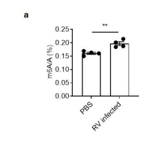
Figure s3. MS analysis of total m6A level in mice ileum. (a) WT and Mettl3 △IEC mice were infected by rotavirus EW strain at 8 days post birth. MS analysis of m6A level in ileum tissue from mice at 2 dpi (mean ± SEM), Statistical significance was determined by Student’s t-test (**P < 0.005)
2) The authors show that Alkbh5 expression is increased when the mice grow up to 3 weeks old. However, the Alkbh5 protein expression changes are missing.
We thank the reviewer for raising this point. We have included the protein expression of ALKBH5 in intestine during the development (see below and Fig. s1). The ALKBH5 protein levels are increased in the intestine along with the age (Fig. s1a, s1b), which is consistent to the changes of mRNA levels of ALKBH5 during the development (Fig. 1d).
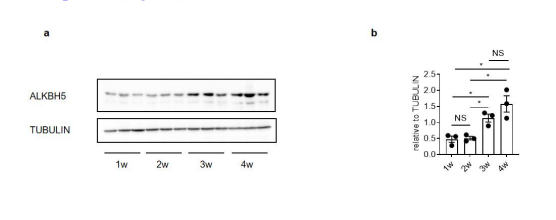
Figure s1. ALKBH5 regulate total m6A level in intestine. (a) Immunoblotting with antibodies target ALKBH5 and TUBULIN in ileum tissues from mice with different ages. (b) Quantitative analysis of (a) (mean ± SEM), Statistical significance was determined by Student’s t-test (*P < 0.05, NS., not significant).
3) The authors claim that m6A declined from 2 to 2 weeks post birth is caused by increased Alkbh5 (Line 110). However, it is not clear if the subtle increase in Alkbh5 mRNA leads to the change in global m6A levels. The author can use ALKBH5-deficient mouse cells to confirm this point.
We thank the reviewer for pointing out an important point. We have included the ALKBH5 over-expression or knock-down data in a mouse IEC cell line MODE-K, to test whether the regulation of Alkbh5 mRNA in IECs leads to the change in global m6A levels.
Over-expression of ALKBH5 in MODE-K cells largely reduced the global m6A level (see below and Fig. s1d). 1. Crispr-mediated knock down of ALKBH5 in MODE-K cells augmented the global m6A level while knock down of another m6A eraser FTO in MODE-K cells didn’t affect the global m6A level (see below and Fig. s10b).
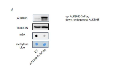
Figure s1. ALKBH5 regulate total m6A level in intestine. (d) Immunoblotting with antibodies target ALKBH5 and TUBULIN in MODE-K cells transfected with pSIN-EV or pSIN-mAlkbh5-3xFlag for 24h. m6A dot blot analysis of total RNA in indicated samples. Methylene blue (MB) staining was the loading control.
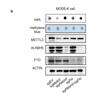
Figure s10. Alkbh5 is the dominant m6A eraser in intestine. (b) m6A dot blot analysis of total RNA in different MODE-K cells. Methylene blue (MB) staining was the loading control.
4) The authors should describe the overall phenotype of IEC-specific METTL3-deficient mice at the steady state. It is important to clarify if the augmented expression of ISG upon METTL3 deficiency is dependent on rotavirus infection. Also, the authors should describe any detectable abnormalities or changes without stimulation.
We actually collaborated another group and found there is a defect in intestinal stem cells in IEC-specific METTL3-deficient mice. However, as RV normally infected IECs in the villi but not in the crypt, and stem cells are not the major producers of IFN/ISGs (Sue E. Crawford et al. Nature reviews disease primers, 2017). The defect in intestinal stem cells will less likely affect the RV infection phenotype. As it is another story that are under review, we tend to not include this part of the data in our manuscript. Moreover, we have crossed Irf7^−/− mice to Mettl3^ΔIEC mice and verified Irf7 mediated induction of ISGs is critical for the anti-viral phenotype in Mettl3^ΔIEC mice.
Our bulk RNA-seq data in IECs showed the augmented expression of ISGs upon METTL3 deficiency in steady state (Fig. 2a). We also found an augmented ISG expression in intestine of METTL3-deficient mice in steady state or early infection of RV (2d) by qPCR. However, as the RV loads in METTL3-deficient mice during the late infection stage are significantly lower than WT mice, thus the inducible ISGs expressions are consequently lower in intestine of METTL3-deficient mice than WT mice in day 4 post infection (Fig. 3f).
5) The finding that IRF7 is targeted by METTL3 is not convincing. First, the authors performed MeRIP-seq and -qPCR experiments only using RNAs from wild-type IECs not from METTL3-deficient cells. It is necessary to show that the modification levels on IRF7 mRNA is indeed reduced upon METTL3 deficiency. Second, it is unclear if MeRIP-seq is properly performed or not, because there is no quality checking figure shown. For instance, the authors can generate metagene plots or gene logos of m6A modified sites to see if there is any consistency with previous reports. Third, in Figure 2h, the authors should show that the change in luciferase activity between wild-type and mutant Irf7-3'UTR reporters is dependent on METTL3 activity by performing METTL3 knockdown or knockout. Also, the authors should describe how they mutagenize the sequences for clarification. Fourth, in Figures 2F and 3C, they showed that IRF7 is upregulated in METTL3-deficient IECs while in Figure 3F, IRF7 is conversely downregulated in METTL3-deficient IECs. This is apparently contradictory to each other.
We appreciate the valuable suggestion provided by the reviewer to improve our manuscript.
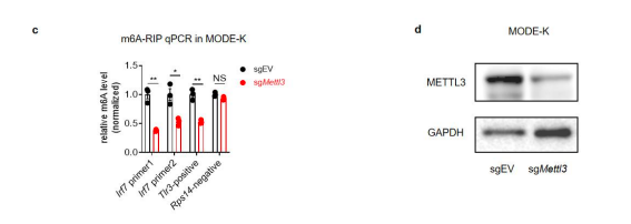
Figure s5. Characterization of m6A modifications on Irf7 mRNA. (c) m6A-RIP-qPCR confirms Irf7 as an m6A-modified gene in IECs. Fragmented RNA of sgEV and sgMettl3 MODE-K cells was incubated with an anti-m6A antibody (Sigma Aldrich ABE572-I). The eluted RNA and input were processed as described in ‘RT-qPCR’section, the data were normalized to the input samples (n=3, mean ± SEM, Statistical significance was determined by Student’s t-test (*P < 0.05, **P < 0.005, NS., not significant). Tlr3 and Rps14 were measured with m6A sites specific qPCR primer as positive control and negative control, Irf7 was measured with predicted m6A sites specific qPCR primers. (d) Knock down efficiency of METTL3 in MODE-K cells.
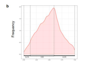
Figure s5. Characterization of m6A modfications on Irf7 mRNA. (b) Metagene plots of m6A modified sites.
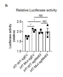
Figure 2. Mettl3 deficiency in intestinal epithelial cells results in decreased m6A deposition on Irf7, and increased interferon responses. (h) Relative luciferase activity of sgEV and sgMettl3 HEK293T cells transfected with pmirGLO-Irf7-3’UTR (Irf7-WT) or pmirGLO-Irf7-3’UTR containing mutated m6A modification sites (Irf7-MUT). The firefly luciferase activity was normalized to Renilla luciferase activity (n=3, mean ± SEM). Statistical significance was determined by Student’s t-tests between genotypes (*P < 0.05, NS., not significant).
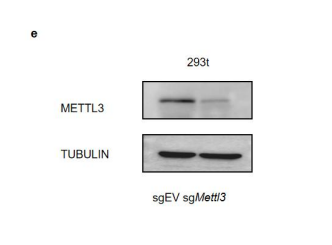
Figure s5. Characterization of m6A modifications on Irf7 mRNA. (e) Knock down efficiency of METTL3 in 293t cells used for luciferase assay.
6) It is unclear if the augmented expression of IRF7 per se upregulates IFN and ISG expression. Since IRF7 exerts its transcriptional activity upon phosphorylation, the authors should examine IRF7 phosphorylation and total protein levels in METTL3-deficient IECs. Also, it is interesting to see if the phosphorylation of TBK1 is augmented or not.
We have provided the phosphorylation and total protein levels of IRF7 and TBK1 in MODE-K cells treated with poly I:C. Both total IRF7 and phosphorylated IRF7 are upregulated in Mettl3-knock down cells compare to control cells (see below and Fig s5f). However, Both total TBK1 and phosphorylated TBK1 remain unchanged (Fig s5f), suggesting the augmented ISGs are less likely due to the activation of the upstream signal of IFN.
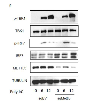
Figure s5. Characterization of m6A modifications on Irf7 mRNA. (f) Western blot analysis of sgEV and sgMettl3 MODE-K cells transfected by lipo3000 with 2ug/ml poly I:C at indicated hours post transfection, at least three replicate experiments were performed.
7) In Figure 3, the authors utilized METTL3 and IRF7 deficient mice to show the contribution of METTL3-mediated IRF7 regulation in rotavirus infection. However, if IRF7 is totally abrogated, IFN production should be greatly impaired as shown in Figure 3A. Thus, it is not surprising to see that the IFN response is diminished. The authors can use heterozygous IRF7 deficient mice instead to check if upregulation of IRF7 under METTL3 deficiency is critical to control rotavirus infection.
We thank the reviewer for pointing out an important issue. However, we checked the IRF7 expression levels in IECs from Irf7^+/+ , Irf7^+/- and Irf7^-/- mice and found that there is no difference between IRF7 levels in IECs from Irf7^+/- mice and that in IECs from Irf7^+/+ mice. Thus, it is not feasible to use heterozygous IRF7 deficient mice to test the idea (Supporting Figure 1).
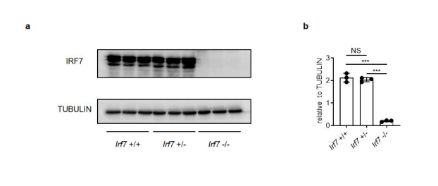
Supporting Figure 1. WT and Irf7 Heterozygous mice show same IRF7 expression level in IECs. (a) IECs from 2-weeks-old Irf7^+/+ , Irf7^+/-, Irf7^-/- mice were isolated. Western blot analysis show IRF7 expression level in different mice. (b) Quantitative analysis of (a) (mean ± SEM), statistical significance was determined by Student’s t-test ( ***P < 0.001, NS., not significant).
8) Given no effect of ALKBH5 knockout on rotavirus infection as shown in Figure 4, it is questionable if ALKBH5 has a profound role in the regulation of m6A in IECs. The authors should determine if m6A modification levels are increased in IECs under ALKBH5 deficiency.
We performed the m6A dot blot assay to detect m6A modification levels in ALKBH5-knock down MODE-K cells and we do find an increase of m6A modification level under ALKBH5 deficiency (see above and Fig s10). No effect of ALKBH5 knockout on rotavirus infection actually puzzled us as well before (Fig.4c, 4d and 4e), until we found RV infection down-regulated ALKBH5 expression in the intestine of WT mice (Fig.4a).
Author Response
Reviewer #1 (Public Review):
This work raises the question of how in plane forces generated at the apical surface of an epithelial cell sheet cause out of plane motion, an important morphogenetic motif. To address this question, a new ontogenetic dominant negative rho1 tool, based on the cry2-CIBN system is presented. The authors use this tool to analyze the well studied biophysical process of ventral furrow formation, and dissect the spatiotemporal requirement of rho1 signaling to modulate myosin accumulation. They separate the effect on morphogenesis into an early phase that becomes significantly slowed down by myosin inhibition, and a late phase where the kinetics is comparable to wild type despite treatment. For interpretation of the data, an older model of cell mechanics treating tissue as a purely elastic material is presented. It fails to reproduce the observations. As a modification, in analogy to buckling of a thin beam under load, a compressive stress exerted by the adjacent ectoderm is introduced. Further analysis of cell behaviors in response to various laser mediated tissue manipulations is presented as support of the proposed mechanism.
Overall, the manuscript addresses an important aspect of morphogenesis. In particular the use of optogenetic tools promises new insights that might be more challenging to achieve with traditional mutant analysis. However, reservations remain with respect to (1) rigor of the analysis, and (2) interpretation and quality of the data in support of the proposed mechanism; this applies in particular to presentation of biophysical observations, including experiment and simulations.
The manuscript adds valuable quantitative data, in particular the findings described in Fig 2ab. However, insufficient analysis are performed to fully support the claims of the manuscript by the data presented.
(I) The manuscript proposes an elasticity based model of tissue mechanics, but provides no experimental evidence in support of this assumption. Many rheology studies performed in a wide range of specimen (including the Drosophila embryo) found a separation of time scales, that shows elasticity is a good approximation of tissue mechanics only for time scales short compared to the process studied here.
We agree with the reviewer that an elasticity-based model of tissue mechanics is a simplification for the actual tissue properties in the real embryos. To provide justification for this simplification, in the revised manuscript, we have cited a previous biophysical study measuring tissue viscoelasticity in early Drosophila embryos (Doubrovinski et al., 2017). Using a magnetic tweezers-based approach, Doubrovinski et al. shows that the lower bound of the decay time of the elastic response is four minutes (the lower limit on the timescales where tissue behaves elastically). In addition, when history dependence of the response is considered, the decay time increases to nine minutes, which is close to the duration of ventral furrow formation (~ 15 – 20 minutes). Therefore, we consider elasticity is a reasonable approximation of tissue mechanics during ventral furrow formation. The elasticity assumption has been widely used in the previously published modeling work to simulate ventral furrow formation (Allena et al., 2010; Conte et al., 2009; Gracia et al., 2019; Heer et al., 2017; Hocevar Brezavšček et al., 2012; Muñoz et al., 2007; Rauzi et al., 2015).The modeling framework used in our current study, which is initially described in Polyakov et al. 2014, successfully predicts the intermediate and final furrow morphologies with a minimal set of active and passive forces without prescribing individual cell shape changes. It is therefore advantageous to use this model to explore the main novel aspect of the folding mechanics underlying ventral furrow formation. We show that the model can recapitulate the binary tissue response to acute myosin inhibition. In addition, it accurately predicts the intermediate furrow morphology at the transitional state and several other morphological properties associated with myosin inhibition. We therefore believe that this minimalistic model captures the central aspect of the physical mechanism underlying mesoderm bistability observed in the experiments.
(II) The manuscript uses a method of micro-dissection to soften cells, but does not provide a clear definition of the concept softening, provides no rational for the methods functioning, and does not provide independent validation. The described treatment might affect cells in many alternative ways to the offered interpretation. This data is the central experimental evidence given in support of the proposed ectoderm compression mechanism, and therefore it is essential to provide a precise physical explanation of the method, and validation of measurements that bolster the conclusion.
We apologize for not explaining the meaning of “softening” clearly in our original manuscript and the rationale for using laser ablation to detect compression. By “softening”, we meant to describe the mechanical status of the cell when the subcellular structures that normally support the mechanical integrity (e.g., cortical actin) are disrupted. We reason that when such a change in mechanical properties happens in a specific region of a tissue that is under compression, the cells in this region should have an impaired ability to resist compression from outside of the region and thereby cause the region to shrink.
Laser ablation has been widely used to measure tensile stresses in cells and tissues by disruption of cells or subcellular structures. The method we used is adapted from previous described protocols, where a femtosecond near infrared laser is used to disrupt subcellular structures for detection of tissue tension (Rauzi et al., 2015; Rauzi et al., 2008).It has been shown that when laser intensity is properly controlled, the treatment can leave the plasma membrane intact but disrupt subcellular structures associated with the plasma membrane, such as adherens junctions and the cortical actomyosin networks (Rauzi et al., 2015; Rauzi et al., 2008).Using a femtosecond near infrared laser, we were able to ablate embryonic tissues that are under tension and observe tissue recoil after laser ablation, suggesting that our approach has disrupted the cortical cytoskeleton in the laser treated region (e.g., Figure 3 and Authors’ Response Figure 1). In these experiments, the lack of damage on the plasma membrane is indicated by the readily recovery of the plasma membrane signal after laser treatment, as well as the lack of bright burn marks on the tissue.
As we noted before, we reasoned that if tissue is compressive, similar laser treatment that generates tissue recoil in tissues under tension should result in tissue shrinking within the laser-treated region. The data presented in our original manuscript demonstrate that tissue shrinking is not a non-specific response to our laser treatment – we did not observe such a response when we treat the tissue during cellularization or within the first five minutes of gastrulation, although identical experimental conditions were used (Original Figure 4). We have also obtained additional evidence that supports the use of tissue shrinking as a readout of tissue compression. We tested our laser ablation approach in Stage 8 – 9 embryos at regions where cells are actively dividing/proliferating, which would expect to generate compressive stresses in the tissue. As we perform laser ablation in this region, we observed shrinking of the treated region, which was distinct from the tensile tissue response (Authors’ Response Figure 1). While this preliminary evidence is encouraging, we agree with the reviewer that further independent validations are needed given that the methods for detecting tissue compression have not been well established in the field. Following the editor’s suggestion, we have removed this experiment from the current manuscript and focus on the characterization of the optogenetic tool and the binary tissue response after acute actomyosin inhibition.
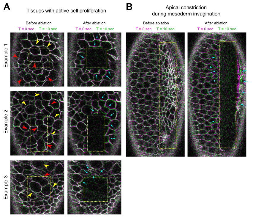
Authors’ Response Figure 1: Laser ablation in regions of tissues with active cell proliferation (a) or undergoing apical constriction (b). The movement of tissues is indicated by overlaying membrane signals (Ecadherin-GFP) at T = 0 sec and at T = 10 sec. T = 0 in the “After ablation” panels marks the time immediately after ablation. (a) Stage 8 – 9 embryos. Multiple cells are in the process of cell division, as indicated by mitotic rounding (yellow arrowheads) or the appearance of cleavage furrows (red arrowheads). Immediately after laser ablation, the surrounding cells moved towards the ablated region (cyan arrows). (b) An embryo undergoing ventral furrow formation. Ablation within the constriction domain results in recoil of the surrounding cells away from the ablated region (cyan arrows).
(III) Mechanical isolation of the mesoderm is a very exciting approach to test the possible involvement of adjacent tissues in folding. Indeed, the authors report a delay of ventral furrow formation. However, there is no evidence provided that (a) the mesoderm is mechanically uncoupled, and (b) that the treatment did not have undesired side effects. For example, a similar procedure (so-called cauterization, see Rauzi 2015) has been used to immobilize cells in the Drosophila embryo. Such an effect could account for the observed delay in furrow formation.
We agree with the reviewer that “mechanical uncoupling” is merely a prediction based on our observation but has not been directly demonstrated. On the other hand, since the purpose of this experiment is to ask whether the presence of the lateral ectoderm is important for the mesoderm to transition between apical constriction and invagination (and our result shows yes), whether the approach we used mechanically uncoupled mesoderm and the ectoderm is no longer an immediately relevant question. We apologize for the imprecise use of the term “mechanically uncoupling” in our original manuscript and we thank the reviewer for pointing this out.
As for the reviewer’s point (b), we have several pieces of evidence indicating that our approach did not cause anchoring of the tissue to the vitelline membrane. The major difference between the approach we used and that used by Rauzi et al. 2015 is the location of the tissue where the laser treatment was imposed. In order to anchor the tissue to the vitelline membrane, Rauzi et al. target the laser to the apical side of the tissue, adjacent to the vitelline membrane. The resulting cauterization of the tissue caused anchoring of the tissue to the vitelline membrane, presumably by fusion of the tissue with the vitelline membrane. In our approach, we used similar type of laser (femtosecond near infrared laser) to perform tissue disruption, but instead of targeting the apical side of the tissue, we targeted the basal region of the invaginating cleavage furrows during cellularization, with the goal to block cell formation. While the laser intensity we used is high enough to cause cauterization of the tissue as indicated by the appearance of bright autofluorescence in the laser treated region, these “burn marks” are not located at the apical side of the cells (Authors’ Response Figure 2a). The lack of “burn marks” on the vitelline membrane in our experiment is in sharp contrast to the result shown in Rauzi et al 2015 (see Authors’ Response Figure 2b for an example from Rauzi et al in comparison to our own data in 2a). Because of the difference in the location of cauterization, we do not expect that the tissue would be fused with the vitelline membrane after our treatment. This is further suggested by the observation that the burn marks can move before the onset of gastrulation, which again indicates that the tissue is not anchored to the vitelline membrane (Authors’ Response Figure 2c).
That being said, we acknowledge that we do not fully understand the impact of the laser treatment on the embryo (e.g., what causes the reduced rate of apical constriction), and more control experiments are required in order to fully describe the tissue response we observed. As suggested by the editor, we decided to remove the ectoderm-ablation experiment from the revised manuscript and focus on the characterization of the optogenetic tool and the binary tissue response after acute actomyosin inhibition.
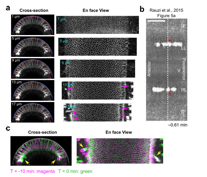
Authors’ Response Figure 2: Laser disruption of cell formation in the lateral ectodermal region. (a) Cross-section and en face views showing the basal location of the “burn marks” after laser disruption in the lateral ectodermal region. No burn marks are observed at the level of the vitelline membrane. Blue and red curves in the cross-section views indicate the vitelline membrane and the position where the projections were made for the en face views. Magenta arrows: burn marks. (b) Figure 5a from Rauzi et al., 2015, clear bright burn marks can be seen from the apical surface view. (c) Overlay of the signal at T = -10 min and 0 min (onset of gastrulation) showing the movement of burn marks before gastrulation (yellow arrows).
(IV) Some panels show two distinct molecules tagged with the same or spectrally overlapping flurophores, that unfortunately localize in similar spatial patterns. This encumbers data validation.
We agree with the reviewer that having two distinct proteins tagged with the same fluorophore is not ideal for understanding the behavior of the tagged proteins, however, it usually does not affect the evaluation of the cell or tissue morphology, as far as the cell membrane is explicitly labeled. For example, in our original Figure 2 (new Figure 4), although GFP is tagged on both CIBN and Sqh, and mCherry is tagged on both CRY2-Rho1DN and Sqh, the cell and tissue morphology is clearly discernable by these markers, which allowed us to evaluate the progression of ventral furrow formation. In the cases where there was a need to evaluate the behavior of a particular molecule (e.g. Sph), we always repeated the experiments in a way such that the molecule of interest is tagged with a distinct fluorophore that does not spectrally overlap with other fluorophores – this often requires the use of an plasma membrane anchored CIBN that is not fluorescently tagged (e.g. Figure 1, Figure 4 – figure supplement 3).
(V) The physical model is a central part for data interpretation. In its current form it is very challenging to follow. It is also critical the system be studied with proper cell aspect ratio, as the elasticity of thin sheets has a well established non-linear thickness dependence.
These are valid critiques of our thin layer physical model (original Figure 5). The original purpose of this model is not to recapitulate the actual furrow morphology or cell shape change observed in the actual embryo, but rather to test the possibility of recapitulating the acceleration in tissue flow during the folding process by combining local constriction and global compression in a spherical (circular in 2D) elastic shell. Developing a dynamic vertex model that contains the realistic cell aspect ratio comparable to the actual cells in the embryo while displaying realistic cellular dynamics during the folding process is nontrivial and need substantial further development of the model. Since the manuscript is now focused on the bistable characteristics of the mesoderm during gastrulation rather than tissue dynamics during the folding process, we decide to leave the dynamics vertex model out of the revised manuscript, as suggested by the editor.
Reviewer #2 (Public Review):
Guo and colleagues aim to unravel the mechanisms driving the fast process of mesoderm invagination in the Drosophila early developing embryo. While cell apical constriction is known to drive ventral furrowing (1st phase), it is still not clear if apical constriction is necessary/sufficient to drive mesoderm internalization (2nd phase) and weather other mechanisms cooperate during this process. By using 1ph optogenetics, the authors cannot test specifically the role of apical constriction but can systematically affect the overall actomyosin network in ventral cells in a time specific fashion (1-minute resolution). In this way, they come to the conclusion that actomyosin contractility is necessary for the 1st phase but not for the 2nd phase of mesoderm invagination. Interestingly, they conclude that the system is bistable. In the second part of this study, the authors test the role of the coupling between mesoderm and ectoderm by using 2D computational modelling and infrared pulsed laser dissection. They propose that the ectoderm can generate compressive forces on the mesoderm facilitating mesoderm internalization (2nd phase).
This project is of interest since it tackles a key morphogenetic process that is necessary for the development of the embryo. The conclusion of 'bistability' resulting from the RhoDN optogenetic experiments (1st part of this study) are well supported and quite interesting. The IR laser experiments used to tackle the coupling between ectoderm and mesoderm (2nd part of the study) are key to support main conclusions, nevertheless their experimental design and results are puzzling. It is not clear what the authors are actually doing to the tissues. The experiments performed in the 2nd part of this study need to be revisited and conclusions eventually softened.
Major comments:
1) The 920 nm laser ablation of ectoderm cells is a key experiment in this study to support the ectoderm compression hypothesis. Nevertheless, this experiment is puzzling: the rationale of the experimental design, the effect of the laser on cells and the interpretation of the results are unclear.
The rationale for the laser ablation experiment designed to test tissue compression is analogous to the widely used laser ablation approach for detecting tissue tension (Rauzi et al., 2015; Rauzi et al., 2008). In typical experiments where laser ablation was used to measure tensile stresses in cells and tissues, ablation of cells or subcellular structures that are under tension results in recoil of surrounding cell/tissue structures. We reasoned that if the tissue is under compression, similar laser treatment should result in shrinking of the laser-treated region, as the cells in the laser-treated region are expected to have an impaired ability to resist compressive stresses from outside of the region.
In our experiment, we used the reduction of the width of the laser treated region within the first 10 sec after laser treatment as the measure for tissue shrinking, which we considered as an indication for the presence of compressive stresses. This tissue response, albeit mild, is not a non-specific tissue response to our laser treatment – we did not observe tissue shrinking when we treat the tissue during cellularization or within the first five minutes of gastrulation, although identical experimental conditions were used. The rate and magnitude of tissue shrinking after laser treatment is determined by multiple factors, including the level of compressive stresses, the difference in cell rigidity before and after laser treatment, and the overall viscosity of the tissue. We acknowledge that the knowledge on these factors is largely lacking, and therefore additional independent validations of our approach are needed to further strengthen our conclusion on the presence of tissue compression. Following the editor’s suggestion, we decided to remove the laser ablation experiment from the current manuscript and focus on the characterization of the optogenetic tool and the binary tissue response after acute actomyosin inhibition.
2) The authors propose to use again 920 nm laser ablation but this time to "physically separate" the two ectoderms from the ventral tissue. This is again a key experiment, but it raises some concerns:
a. "Physical separation" would need to be demonstrated (e.g., EM after laser ablation). From Fig. 6b it is clear that IR laser ablation results in prominent auto-fluorescent zones. This has been already reported in previous work (De Medeiros G. et al. Scientifc Reports 2020) showing that high power and sustained IR fs laser targeting produces auto-fluorescence and highly electron-dense structures in the early developing Drosophila embryo. This process is referred to laser cauterization that does not induce separation between tissues. This structures eventually displace together with the lateral tissue (also shown in Fig.6 b). b. This strong laser "treatment", that should be ectoderm specific, results in perturbation of other non-ectoderm related processes (e.g., mesoderm apical constriction as shown by the authors). This can support the idea that many other processes are affected and that in general this laser heating "treatment" has global effects. These results might invalidate the conclusion proposed by the authors.
These are both valid critiques. As for the reviewer’s point “a”, we agree with the reviewer that a “physical separation” of the mesoderm from the ectoderm has not been rigorously demonstrated in our original manuscript. As detailed in our response to reviewer #1 comment #3, since the purpose of this experiment is to ask whether the presence of the lateral ectoderm is important for the mesoderm to transition between apical constriction and invagination (and our result shows yes), whether the approach we used physically separated the mesoderm and the ectoderm is no longer an immediately relevant question. We apologize for the vague use of “physical separation” in our original manuscript and we thank the reviewer for pointing this out.
To address the reviewer’s point “b” and to ask whether the laser treatment used in our experiment has a global effect, we performed a control experiment where we treated the yolk region of the embryo with the identical approach. Despite the appearance of burn marks in the treated yolk region, mesoderm invagination proceeded largely normally under this condition, with a mild reduction in the rate of furrow invagination (Authors’ Response Figure 3). Therefore, the prominent delay in the transitional state we observed after disruption of lateral ectoderm (Original Figure 6) is not likely caused by non-specific laser heating effect. In addition, in both the yolk-ablation and the ectoderm-ablation experiments, cellularization occurred normally outside of the laser-treated regions, in further support of the lack of strong non-specific effect from our laser treatment. That being said, we acknowledge that we do not fully understand the impact of the laser treatment on the embryo (e.g., what causes the reduced rate of apical constriction), and more control experiments are required in order to fully describe the tissue response we observed. As suggested by the editor, we decided to remove the ectoderm-ablation experiment from the revised manuscript and focus on the characterization of the optogenetic tool and the binary tissue response after acute actomyosin inhibition.
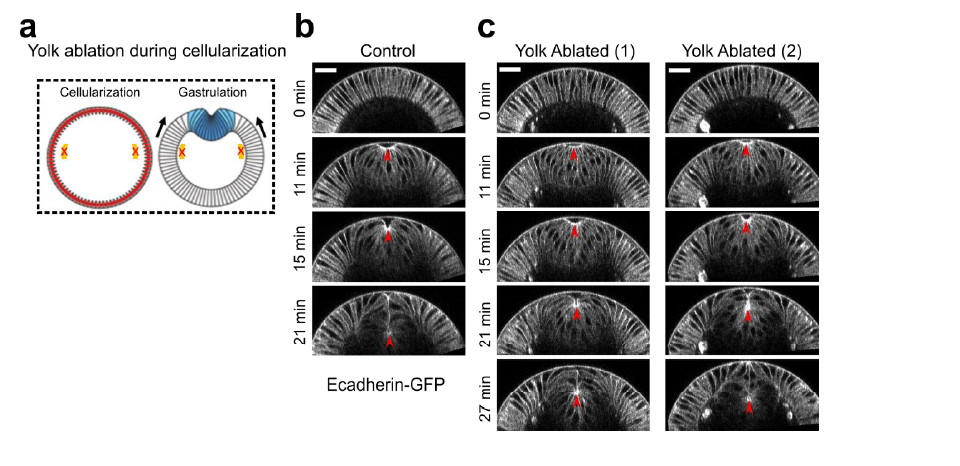
Authors’ Response Figure 3. Laser treatment in the yolk region of the embryo. (a) Cartoon depicting the position of laser treatment. Similar laser condition was used as described in the original Figure 6. Laser ablation was performed during cellularization and the treated embryo was imaged during gastrulation. (b) An example control embryo without laser treatment. (d-e) Two examples showing ventral furrow formation after laser treatment in the yolk region. Only a mild delay in furrow invagination was observed. Red arrowheads indicate the invagination front. Scale bar: 25μm.
Reviewer #3 (Public Review):
The authors address how contractile forces near the apical surface of a cell sheet drive out-of-plane bending of the sheet. To determine whether actomyosin contractility is required throughout the folding process and to identify potential actomyosin independent contributions for invagination, they develop an optogenetic-mediated inhibition of myosin and show that myosin contractility is critical to prevent tissue relaxation during the early stage of folding but is dispensable for the deepening of the invagination. Their results support the idea that the mesoderm is mechanically bistable during gastrulation. They propose that this mechanical bistability arises from an in-plane compression from the surrounding ectoderm and that mesoderm invagination is achieved through the combination of apical constriction and tissue compression. Regarding global message of the manuscript, I have two main critics. The authors consider their work as the first to prove that there is a additional mechanism to apical constriction leading to invagination. This is not true. First, the fact that the ectoderm could exert a compressive force on the invaginating mesoderm is not new and has been not only proposed, but tested previously (Rauzi and Leptin, 2015). Second, several recent publications demonstrated that on top of apical constriction, lateral forces were also required for the invagination and the authors ignore these data (Gracia et al, 2019 ; John et al, 2021).
We thank the reviewer for this important comment. In the original Introduction, we have mentioned several previous studies that suggest the presence of additional mechanisms to apical constriction during ventral furrow formation. We stated: “The observation that the maximal rate of apical constriction and the maximal rate of tissue invagination occur at distinct times suggests that apical constriction does not directly cause tissue invagination (Polyakov et al., 2014; Rauzi et al., 2015). A number of computational models also predict that mesoderm invagination requires additional mechanical input, such as “pushing” forces from the surrounding ectodermal tissues, but experimental evidence for this additional mechanical input remains sparse (Munoz et al., 2007; Conte et al., 2009; Allena et al., 2010; Brodland et al., 2010).”
To address the reviewer’s comment, in the revised manuscript, we expanded this paragraph to further elaborate the previous contributions: “However, accumulating evidence suggests that apical constriction does not directly drive invagination during the shortening phase. First, it has been observed that the maximal rate of apical constriction (or cell lengthening) and the maximal rate of tissue invagination occur at distinct times (Polyakov et al., 2014; Rauzi et al., 2015). Second, it has been previously proposed, and more recently experimentally demonstrated, that myosin accumulated at the lateral membranes of constricting cells (‘lateral myosin’) facilitates furrow invagination by exerting tension along the apical-basal axis of the cell (Brodland et al., 2010; Conte et al., 2012; Gracia et al., 2019; John and Rauzi, 2021). Finally, a number of computational models predict that mesoderm invagination requires additional mechanical input from outside of the mesoderm, such as “pushing” forces from the surrounding ectodermal tissue (Munoz et al., 2007; Conte et al., 2009; Allena et al., 2010; Brodland et al., 2010). These models are in line with the finding that blocking the movement of the lateral ectoderm by laser cauterization inhibits mesoderm invagination (Rauzi et al., 2015). A similar disruption of ventral furrow formation can also be achieved by increasing actomyosin contractility in the lateral ectoderm (Perez-Mockus et al., 2017). While these pioneer studies highlight the importance of cross-tissue coordination during mesoderm invagination, the actual mechanical mechanism that drives the folding of the mesodermal epithelium and the potential role of the surrounding ectodermal tissue remain to be elucidated.”
One of the motivations for us to develop experimental approaches to detect compression in the ectoderm (original Figure 4) and to disrupt the ectoderm (original Figure 6) is the lack of direct evidence demonstrating the mechanical contribution of the ectoderm to mesoderm invagination. Several studies have shown that manipulations of the ectodermal tissue can impair ventral furrow formation. One study shows that preventing the movement of the lateral ectoderm, by anchoring ectodermal cell apices to the vitelline membrane, blocks ventral furrow invagination(Rauzi et al., 2015). Another study shows that upregulation of apical myosin contractility in the lateral ectodermal tissues can inhibit or even reverse the furrow invagination process (Perez-Mockus et al., 2017). These results indicate that an increase in the resistance to mesoderm movement can impair mesoderm invagination. However, this would be expected even if the ectoderm does not provide active mechanical input to facilitate mesoderm invagination. Therefore, these experiments, while very informative, did not provide direct evidence for a role of ectodermal compression in mesoderm invagination.
Another motivation for us to examine potential mechanisms outside of the mesoderm is the observation that ventral furrow invagination continues even when both apical myosin and lateral myosin are disrupted after Ttrans (Late Group embryos). This result indicates that factors other than apical or lateral myosin must be responsible for the invagination of the furrow in Late Group embryos. In the revised manuscript, we used a modeling approach to demonstrate that lateral myosin and ectodermal compression may function in parallel to promote the invagination of the ventral furrow (Figure 7). In the revised Discussion, we propose that “ventral furrow formation is mediated through a joint action of multiple mechanical inputs. Apical constriction drives initial indentation of ventral furrow, which primes the tissue for folding, whereas the subsequent rapid folding of the furrow is promoted by bistable characteristic of the mesoderm and by lateral myosin contractions in the constricting cells.”
They generated an optogenetic tool, "Opto-Rho1DN", to inhibit Rho1 through light-dependent plasma membrane recruitment of a dominant negative form of Rho1 (Rho1DN). The specificity of local inactivation of Myosin was tested on apical myosin before and during invagination. They observed a strong reduction of Myosin II recruitment and a phenotype that mimicks Rok inhibition. They found that acute loss of myosin contractility during most of the lengthening phase results in immediate relaxation of the constricted tissue, but similar treatment near or after the lengthening-shortening transition does not impede invagination. They conclude that the second part of furrow invagination is not due to myosin activities at the apical or lateral cortices of the mesodermal cells and that actomyosin contractility is required in the early but not the late phase of furrow formation. This part regarding the temporal requirement of Myosin during invagination brings novelty in the field since it has never been tested before.
We thank the reviewer for the comment on the novelty of our work.
They observe that ectodermal cells shorten their apico-basal axis prior to Ttrans, and that compression from the ectoderm is independent of ventral furrow formation since it still occurs even if invagination is inhibited.
They further develop two types of simulations to test theoretically the importance of compressive stress in the invagination process. The theoretical part would need to be further developed and discussed. They would need to integrate all the different components that have been shown to be essential for the invagination (not only apical constriction) and the dynamic aspect of the vertex model has to be clearly explained.
We thank the reviewer for the suggestions on the modeling parts. In the energy-based vertex model (the Polyakov model, original Figure 3), two previously identified mechanisms, apical constriction and basal relaxation, have been implemented in the model to drive lengthening-shortening cell shape change and furrow invagination. Following the reviewer’s suggestions, we have modified the Polyakov model to include additional mechanisms that have been shown to facilitate ventral furrow invagination. In particular, we focused our analysis on the role of lateral myosin in the constricting cells on furrow invagination (Figure 7). Please refer to our response to the combined comments for details (in the section “ Additional modeling analysis to test the known mechanisms for mesoderm invagination”).
As for the dynamic vertex model presented in our original manuscript (original Figure 5), as detailed in our response to Reviewer #1’s comment #5, since the revised manuscript is focused on the bistable characteristics of the mesoderm during gastrulation rather than tissue dynamics during the folding process, we decide to leave this part out of our revised manuscript as suggested by the editor.
Author Response
Reviewer #1 (Public Review):
This thorough study expands our understanding of BMP signaling, a conserved developmental pathway, involved in processes diverse such as body patterning and neurogenesis. The authors applied multiple, state-of-art strategies to the anthozoan Nematostella vectensis in order to first identify the direct BMP signaling targets - bound by the activated pSMAD1/5 protein - and then dissect the role of a novel pSMAD1/5 gradient modulator, zwim4-6. The list of target genes features multiple developmental regulators, many of which are bilaterally expressed, and which are notably shared between Drosophila and Xenopus. The analysis identified in particular zswim4-6 a novel nuclear modulator of the BMP pathway conserved also in vertebrates. A combination of both loss-of-function (injection of antisense morpholino oligonucleotide, CRISPR/Cas9 knockout, expression of dominant negative) and gain-of-function assays, and of transcriptome sequencing identified that zwim acts as a transcriptional repression of BMP signaling. Functional manipulation of zswim5 in zebrafish shows a conserved role in modulating BMP signaling in a vertebrate.
The particular strength of the study lies in the careful and thorough analysis performed. This is solid developmental work, where one clear biological question is progressively dissected, with the most appropriate tools. The functional results are further validated by alternative approaches. Data is clearly presented and methods are detailed. I have a couple of comments.
1) I was intrigued - as the authors - by the fact that the ChiP-Seq did not identify any known BMP ligand bound by pSMAD1/5. Are these genes found in the published ChiP-Seq data of the other species used for the comparative analysis? One hypothesis could be that there is a change in the regulatory interactions and that the initial set-up of the gradient requires indeed a feedback loop, which is then turned off at later gastrula. In this case, immunoprecipitation at early gastrula, prior to the set-up of the pSMAD1/5 gradient, could reveal a different scenario. Alternately, the regulation could be indirect, for example, through RGM, an additional regulator of BMP signaling expressed on the side of lower BMP activity, which is among the targets of the ChiP-Seq. This aspect could be discussed. Additionally, even if this is perhaps outside the scope of this study, I think it would be informative to further assess the effect of ZSWIM manipulation on RGM (and vice versa).
Indeed, BMP genes are direct BMP signaling targets in Drosophila (dpp) (Deignan et al., 2016, https://doi.org/10.1371/journal.pgen.1006164) and frog (bmp2, bmp4, bmp5, bmp7) (Stevens et al., 2021, https://doi.org/10.1242/dev.145789). Of all these ligands, only the dorsally expressed Xenopus bmp2 is repressed by BMP signaling, while another dorsally expressed Xenopus BMP gene admp is not among the direct targets. All other BMP genes listed here are expressed in the pMad/pSMAD1/5/8-positive domain and are activated by BMP signaling.
In Nematostella, we do not find BMP genes among the ChIP-Seq targets, but this is not that surprising considering the dynamics of the bmp2/4, bmp5-8 and chordin expression, as well as the location of the pSMAD1/5-positive cells. In late gastrulae/early planulae, Chordin appears to be shuttling BMP2/4 and BMP5-8 away from their production source and over to the gdf5-like side of the directive axis (Genikhovich et al., 2015; Leclere and Rentsch, 2014). By 4 dpf, chordin expression stops, and BMP2/4 and BMP5-8 start to be both expressed AND signal in the mesenteries. If bmp2/4 and bmp5-8 expression were directly suppressed by pSMAD1/5 (as is the case chordin or rgm expression), this mesenterial expression would not be possible. Therefore, in our opinion, it is most likely that at late gastrula and early planula the regulation of bmp2/4 and bmp5-8 expression by BMP signaling is indirect. We do not have an explanation for why gdf5-like (another BMP gene expressed on the “high pSMAD1/5” side) is not retrieved as a direct BMP target in our ChIP data. Since we do not understand well enough how BMP gene expression is regulated, we do not discuss this at length in the manuscript.
As the Reviewer suggested, we analyzed the effect of ZSWIM4-6 KD on the expression of rgm. Expectedly, since it is expressed on the “low BMP side”, its expression was strongly expanded (Figure 6 - Figure Supplement 4)
2) I do not fully understand the rationale behind the choice of performing the comparative assays in zebrafish: as the conservation was initially identified in Xenopus, I would have expected the experiment to be performed in frog. Furthermore, reading the phylogeny (Figure 4A), it is not obvious to me why ZSWIM5 was chosen for the assay (over the other paralog ZSWIM6). Could the Authors comment on this experiment further?
The comparison was done in zebrafish because we were planning to generate zswim5 mutants, whose analysis is currently in progress. ZSWIM6 is not expressed at the developmental stages we were interested in, while ZSWIM5 was, based on available zebrafish expression data (White et al., 2017):
Reviewer #2 (Public Review):
The authors provide a nice resource of putative direct BMP target genes in Nematostella vectensis by performing ChIP-seq with an anti-pSmad1/5 antibody, while also performing bulk RNA-seq with BMP2/4 or GDF5 knockdown embryos. Genes that exhibit pSmad1/5 binding and have changes in transcription levels after BMP signaling loss were further annotated to identify those with conserved BMP response elements (BREs). Further characterization of one of the direct BMP target genes (zswim4-6) was performed by examining how expression changed following BMP receptor or ligand loss of function, as well as how loss or gain of function of zswim4-6 affected development and BMP signaling. The authors concluded that zswim4-6 modulates BMP signaling activity and likely acts as a pSMAD1/5 dependent co-repressor. However, the mechanism by which zswim4-6 affects the BMP gradient or interacts with pSMAD1/5 to repress target genes is not clear. The authors test the activity of a zswim4-6 homologue in zebrafish (zswim5) by over-expressing mRNA and find that pSMAD1/5/9 labeling is reduced and that embryos have a phenotype suggesting loss of BMP signaling, and conclude that zswim4-6 is a conserved regulator of BMP signaling. This conclusion needs further support to confirm BMP loss of function phenotypes in zswim5 over-expression embryos.
Major comments
1) The BMP direct target comparison was performed between Nematostella, Drosophila, and Xenopus, but not with existing data from zebrafish (Greenfeld 2021, Plos Biol). Given the functional analysis with zebrafish later in the paper it would be nice to see if there are conserved direct target genes in zebrafish, and in particular, is zswim5 (or other zswim genes) are direct targets. Since conservation of zswim4-6 as a direct BMP target between Nematostella and Xenopus seemed to be part of the rationale for further functional analysis, it would also be nice to know if this is a conserved target in zebrafish.
Thank you for the suggestion. In the paper by Greenfeld et al., 2021, zebrafish zswim5 was downregulated approximately 2.4x in the bmp7 mutant at 6 hpf, while zswim6 was barely expressed and not affected at this stage. We added this information to the text of the manuscript. Expression of several other zebrafish zswim genes was also affected in the bmp7 mutant, but these genes do not appear relevant for our study since their corresponding orthologs are not identified as pSMAD1/5 ChIP-Seq targets in Nematostella. Notably, zebrafish zzswim5 is not clearly differentially expressed in BMP or Chd overexpression conditions (See Supplementary file 1 in Rogers et al. 2020). Importantly, in the paper, we wanted to compare ChiP-Seq data with ChIP-Seq data, however, unfortunately, no ChIP-Seq data for pSMAD1/5/8 is currently available for zebrafish, thus precluding comparisons.
Related to this, in the discussion it is mentioned that zswim4/6 is also a direct BMP target in mouse hair follicle cells, but it wasn't obvious from looking at the supplemental data in that paper where this was drawn from.
Please see Supplementary Table 1, second Excel sheet labeled “Mx ChIP_Seq” in Genander et al., 2014, https://doi.org/10.1016/j.stem.2014.09.009. Zswim4 has a single pSMAD1 peak associated with it, Zswim6 has two.
2) The loss of zswim4-6 function via MO injection results in changes to pSmad1/5 staining, including a reduction in intensity in the endoderm and gain of intensity in the ectoderm, while over-expression results in a loss of intensity in the ectoderm and no apparent change in the endoderm. While this is interesting, it is not clear how zswim4-6 is functioning to modify BMP signaling, and how this might explain differential effects in ectoderm vs. endoderm. Is the assumption that the mechanism involves repression of chordin? And if so one could test the double knockdown of zswim4-6 and chordin and look for the rescue of pSad1/5 levels or morphological phenotype.
We do not think that the mechanism of the ZSWIM4-6 action is via repression of Chordin. As loss of chordin leads to the loss of pSMAD1/5 in Nematostella (Genikhovich et al., 2015), the proposed experiment is, unfortunately, not feasible to test this hypothesis. Currently, we see two distinct effects of the modulation of zswim4-6 expression. First, it affects the pSMAD1/5 gradient, possibly by destabilizing nuclear SMAD1/5, as has been proposed by Wang et al., 2022 for the vertebrate Zswim4. This is in line with our results shown on Fig. 6C-F’ and Fig. 6-Figure supplement 3. In our opinion, the reaction of the genes expressed on the “high BMP” side of the directive axis to the overexpression or KD of ZSWIM4-6 (Fig. 6I-K’, 6N-P’) can be explained by these changes in the pSMAD1/5 signaling intensity. Secondly, zswim4-6 appears to promote pSMAD1/5-mediated gene repression. This is in line with the reaction of the genes expressed on the “low BMP” side of the directive axis (Fig. 6G-H’, 6L-M’, Fig. 6-Figure Supplement 4). These genes are repressed by BMP signaling, but they expand their expression upon zswim4-6 KD in spite of the increased pSMAD1/5. Our ChiP experiment (Fig. 6Q) supports this view.
3) Several experiments are done to determine how zswim4-6 expression responds to the loss of function of different BMP ligands and receptors, with the conclusion being that swim4-6 is a BMP2/4 target but not a GDF5 target, with a lot of the discussion dedicated to this as well. However, the authors show a binary response to the loss of BMP2/4 function, where zswim4-6 is expressed normally until pSmad1/5 levels drop low enough, at which point expression is lost. Since the authors also show that GDF5 morphants do not have as strong a reduction in pSmad1/5 levels compared to BMP2/4 morphants, perhaps GDF5 plays a positive but redundant role in swim4-6 expression. To test this possibility the authors could inject suboptimal doses of BMP2/4 MO with GDF5 MO and look for synergy in the loss of zswim4-6 expression.
Thanks for this great suggestion! We performed this experiment (Fig. 5H’’-L) and indeed, a suboptimal dose of BMP2/4MO + GDF5lMO results in a complete radialization of the embryo and abolished zswim4–6, similar to the effect of a high dose of BMP2/4. This result suggests that rather than being a ligand-specific signaling function, GDF5-like signaling alone still provides sufficiently high pSmad1/5 levels to activate zswim4-6 expression to apparent wildtype levels, demonstrating the sensitivity of this gene to even very low amounts of BMP signaling.
4) The zswim4-6 morphant embryos show increased expression of zswim4-6 mRNA, which is said to indicate that zswim4-6 negatively regulates its own expression. However in zebrafish translation blocking MOs can sometimes stabilize target transcripts, causing an artifact that can be mistakenly assumed to be increased transcription (https://www.ncbi.nlm.nih.gov/pmc/articles/PMC7162184/). Some additional controls here would be warranted for making this conclusion.
Thanks for raising this important experimental consideration. To-date, we do not have any evidence for MO-mediated transcript stabilization in Nematostella, and we have not found such data in the literature on models other than zebrafish. mRNA stabilization by the MO also seemed unlikely because we were unable to KD zswim4-6 using several independent shRNAs - an effect we frequently observe with genes, whose activity negatively regulates their own expression. However, to test the possibility that zswim4-6MO binding stabilizes zswim4-6 mRNA, we injected mRNA containing the zswim4-6MO recognition sequence followed by the mCherry coding sequence (zswim4-6MO-mCherrry) with either zswim4-6MO or control MO. We could clearly detect mCherry fluorescence at 1 dpf if control MO was co-injected with the mRNA, but not if zswim4-6MO was coninjected with the mRNA. At 2 dpf (the stage at which we showed upregulation of zswim4-6 upon zswim4-6MO injection on Fig. 6I-I’), zswim4-6MO-mCherrry mRNA was undetectable by in situ hybridization with our standard FITC-labeled mCherry probe independent of whether zswim4-6MO-mCherrry mRNA was co-injected with the control MO or ZSWIM4-6MO, while hybridization with the FITC-labeled FoxA probe worked perfectly.
Author response image 1.
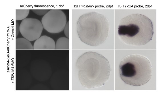
We are currently offering two alternative hypothesis for the observed increase in zswim4-6 levels in the paper rather than stating explicitly that ZSWIM4-6 negatively regulates its own expression: “The KD of zswim4-6 translation resulted in a strong upregulation of zswim4-6 transcription, especially in the ectoderm, suggesting that ZSWIM4-6 might either act as its own transcriptional repressor or that zswim4-6 transcription reacts to the increased ectodermal pSMAD1/5 (Fig. 6I-I’).” Given the sensitivity of zswim4-6 to even the weakest pSMAD1/5 signal (zswim4/6 is expressed upon GDF5-like KD, which drastically reduces pSMAD1/5 signaling intensity (see Fig. 1 and 2 in Genikhovich et al., 2015, http://doi.org/10.1016/j.celrep.2015.02.035 and Fig. 6-Figure supplement 3 of this paper), the latter option (that it reacts to the increased ectodermal pSMAD1/5) is, in our opinion, clearly the more probable one.
5) Zswim4-6 is proposed to be a co-repressor of pSmad1/5 targets based on the occupancy of zswim4-6 at the chordin BRE (which is normally repressed by BMP signaling) and lack of occupancy at the gremlin BRE (normally activated by BMP signaling). This is a promising preliminary result but is based only on the analysis of two genes. Since the authors identified BREs in other direct target genes, examining more genes would better support the model.
We suggest that ZSWIM4-6 may be a co-repressor of pSMAD1/5 targets because it is a nuclear protein (Fig. 4G), whose knockdown results in the expansion of the ectodermal expression of several genes repressed by pSMAD1/5 in spite of the expansion of pSMAD1/5 itself (Fig. 6G-H’, 6L-M’, Fig. 6-Figure Supplement 4). Our limited ChIP analysis supports this idea by showing that ZSWIM4-6 is bound to the pSMAD1/5 site of chordin (repressed by pSMAD1/5) but not on gremlin (activated by pSMAD1/5). We agree that adding the analysis of more targets in order to challenge our hypothesis would be good. However, given technical limitations (having to inject many thousands of eggs with the EF1a::ZSWIM4-6-GFP plasmid in order to get enough nuclei to extract sufficient immunoprecipitated chromatin for qPCR on 3 genes (chordin, gremlin, GAPDH) for each biological replicate, it is currently unfortunately not feasible to test more genes. It will be of great interest for follow up studies to generate a knock-in line with tagged zswim4-6 to analyze target binding on a genome-wide scale. We stress in the discussion that currently the power of our conclusion is low.
6) The rationale for further examination of zswim4-6 function in Nematostella was based in part on it being a conserved direct BMP target in Nematostella and Xenopus. The analysis of zebrafish zswim5 function however does not examine whether zswim5 is a BMP target gene (direct or indirect). BMP inhibition followed by an in situ hybridization for zswim5 would establish whether its expression is activated downstream of BMP.
In the paper by Greenfeld et al., 2021, zebrafish zswim5 was downregulated approximately 2.4x in the bmp7 mutant at 6 hpf. However, this gene was not among the 57 genes, which were considered to be direct BMP targets because their expression was affected by bmp7 mRNA injection into cycloheximide-treated bmp7 mutants (Greenfeld et al., 2021). We added this information to the text of the manuscript.
7) Although there is a reduction in pSmad1/5/9 staining in zebrafish injected with zswim5 mRNA, it is difficult to tell whether the resulting morphological phenotypes closely resemble zebrafish with BMP pathway mutations (such as bmp2b). More analysis is warranted here to determine whether stereotypical BMP loss of function phenotypes are observed, such as dorsalization of the mesoderm and loss of ventral tail fin.
We agree, and we have tuned down all zebrafish arguments. Analyses of zswim5 mutants are currently ongoing.
Author Response
Reviewer #3 (Public Review):
1) Validation of reagents: The authors generated a pY1230 Afadin antibody claiming that (page 6) "this new antibody is specific to tyrosine phosphorylated Afadin, and that pY1230 is targeted for dephosphorylation by PTPRK, in a D2-domain dependent manner". The WB in Fig 1B shows a lot of background, two main bands are visible which both diminish in intensity in ICT WT pervanadate-treated MCF10A cell lysates. The claim that the developed peptide antibody is selective for pY1230 in Afadin would need to be substantiated, for instance by pull down studies analysed by pY-MS to substantiate a claim of antibody specificity for this site. However, for the current study it would be sufficient to demonstrate that pY1230 is indeed the dephosphorylated site. I suggest therefore including a site directed mutant (Y1230F) that would confirm dephosphorylation at this site and the ability of the antibody recognizing the phosphorylation state at this position.
We would like this antibody to be a useful and freely accessible tool in the field and have taken on board the request for additional validation. To this end we have significantly expanded Supplementary Figure 2 (now Figure 1 - figure supplement 2) and included a dedicated section of the results as follows: 1. We have now included information about all of the Afadin antibodies used in this study, since Afadin(BD) appears to be sensitive to phosphorylation (Figure 1 - figure supplement 2A). 2. We have demonstrated that the Afadin pY1230 antibody detects an upregulated band in PTPRK KO MCF10A cells, consistent with our previous tyrosine phosphoproteomics (Figure 1 - figure supplement 2B). This indicates that the antibody can be used to detect endogenous Afadin phosphorylation. 3. We have included two new knock down experiments demonstrating the recognition of Afadin by our antibody (Figure 1 - figure supplement 2C). There appear to be two Afadin isoforms recognised in HEK293T cells by both the BD and pY1230 antibody, consistent with previous reports (Umeda et al. MBoC, 2015). We have highlighted these in the figure. 4. We have performed mutagenesis to demonstrate the specificity of the antibody. We tagged Afadin with a fluorescent protein tag, reasoning that it would cause a shift in molecular weight that could be resolved by SDS PAGE, as is the case. We noted that the phosphopeptide used spans an additional tyrosine, Y1226, which has been detected as phosphorylated (although to a much lower extent than Y1230) on Phosphosite plus. The data clearly show that Afadin cannot be phosphorylated when Y1230 is mutated to a phenylalanine (compared to CIP control), indicating that this is the predominant site recognised by the antibody. In addition, the endogenous pervanadate-stimulated signal is completely abolished by CIP treatment (Figure 1 - figure supplement 2D). 5. We have included densitometric quantification of the dephosphorylation assay shown in Figure 1B, which was part of a time course and shows preferential dephosphorylation by the PTPRK ICD compared to the PTPRK D1. The signal stops declining with time, which could indicate antibody background, or an inaccessible pool of Afadin-pY1230 (Figure 1 - figure supplement 2E). 6. To further demonstrate that this site is modulated by PTPRK in post-confluent cells, we have used doxycycline (dox)-inducible cell lines generated in Fearnley et al, 2019. Upon treatment with 500 ng/ml Dox for 48 hours PTPRK is induced to lower levels than wildtype, however, normalized quantification of the Afadin pY1230 against the Afadin (CST) signal clearly indicates downregulation by PTPRK WT, but not the catalytically inactive mutant (Figure 1 - figure supplement 2F and 2G). Together these data strengthen our assertion that this antibody recognises endogenously phosphorylated Afadin at site Y1230, which is modulated in vitro and in cells by PTPRK phosphatase activity. For clarity, we have highlighted and annotated the relevant bands in figures. We have also included identifiers for each Afadin total antibody was used in particular experiments.
2) The authors claim that a short, 63-residue predicted coiled coil (CC) region, is both necessary and sufficient for binding to the PTPRK-ICD. The region is predicted to have alpha-helical structure and as a consequence, a helical structure has been used in the docking model. Considering that the authors recombinantly expressed this region in bacteria, it would be experimentally simple confirming the alpha-helical structure of the segment by CD or NMR spectroscopy.
To clarify, the helical structure in the docking model was independently predicted by several sequence and structural analysis programmes including AlphaFold2, RobettaFold, NetSurfP and as annotated in Uniprot (as a coiled coil). We did not stipulate prior to the AF2 prediction that it was helical. Isolated short peptides frequently adopt helical structure, therefore prediction of a helix within the context of the full Afadin sequence is, in our opinion, stronger evidence than CD of an isolated fragment.
3) Only two mutants have been introduced into PTPRK-ICD to map the Afadin interaction site. One of the mutations changes a possibly structurally important residues (glycine) into a histidine. Even though this residue is present in PTPRM, it does not exclude that the D2 domain no longer functionally folds. Also the second mutation represents a large change in chemical properties and the other 2 predicted residues have not been investigated.
The residues that were selected for mutation are all localised to the protein surface and therefore are unlikely to be involved in stable folding of PTPRK. In support of the correct folding of the mutated PTPRK, we include in Figure 1 below SEC elution traces for wild-type and mutant D2 showing that they elute as single symmetric peaks at the same elution volume as the WT protein. This is consistent with them having a similar shape and size, and not being aggregated or unfolded.
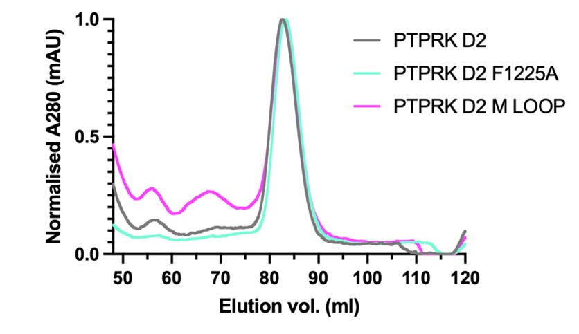
Figure 1. PTPRK-D2 wild-type and mutant preparative SEC elution profiles. A280nm has been normalised to help illustrate that the different proteins elute at the same volume. The main peak from these samples was used for binding assays in the main paper.
Furthermore, the yield for the double mutant was very high (4 mg of pure protein from a 2 L culture, see A280 value in graph below), whereas poorly folded proteins tend to have significantly reduced yields. This protein was also very stable over time whereas unfolded proteins tend to degrade during or following purification.
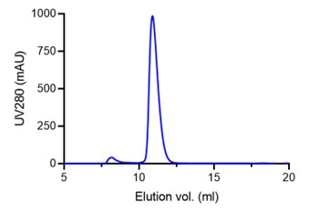
Figure 2. Analytical SEC elution profile for the PTPRK-D2 DM construct showing the very high yield consistent with a well-folded, stable protein.
Finally, we have carried out thermal melt curves of the WT and mutant PTPRK D2 domains showing that they all possess melting temperatures between 39.3°C and 41.7°C, supporting that they are all equivalently folded. We include these data as an additional Supplementary Figure (Figure 4 - figure supplement 3) in the paper.
4) The interface on the Afadin substrate has not been investigated apart from deleting the entire CC or a central charge cluster. Based on the docking model the authors must have identified key positions of this interaction that could be mutated to confirm the proposed interaction site.
We have now made and tested several additional mutations within both the Afadin-CC and PTPRK-D2 domains to further validate the AF2 predicted model of the complex.
For Afadin-CC we introduced several single and double mutations along the helix including residues predicted to be in the interface and residues distal from the interface. These mutations and the pulldown with PTPRK are described in the text and are included as additional panels to a modified Figure 3. All mutations have the expected effect on the interaction based on the predicted complex structure. To help illustrate the positions of these mutations we have also included a figure of the interface with the residues highlighted.
For the PTPRK-D2 we have also introduced two new mutations, one buried in the interface (F1225A) and one on the edge of the interface encompassing a loop that is different in PTPRM (labelled the M-loop). GST-Afadin WT protein was bound to GSH beads and tested for their ability to pulldown WT and mutated PTPRK. These new mutations (illustrated in the new Figure 4 – figure supplement 2) further support the model prediction. F1225A almost completely abolishes binding as predicted, while the M-loop retains binding. These mutations and their effects are now described in the main text and the pull-down data, including controls and retesting of the original DM mutant, are included as panel H in a newly modified Figure 4 focussed solely on the PTPRK interface.
5) A minor point is that ITC experiments have not been run long enough to determine the baseline of interaction heats. In addition, as large and polar proteins were used in this experiment, a blank titration would be required to rule out that dilution heats effect the determined affinities.
All control experiments including buffer into buffer, Afadin into buffer and buffer into PTPRK were carried out at the same time as the main binding experiment and are shown below overlaid with the binding curve. These demonstrate the very small dilution heats consistent with excellent buffer matching of the samples.
We were able to obtain excellent fits to the titration curves by fitting 1:1 binding with a calculated linear baseline (see Figure 2B,D). Very similar results were obtained by fitting to the sum (‘composite’) of fitted linear baselines obtained for the three control experiments for each titration.
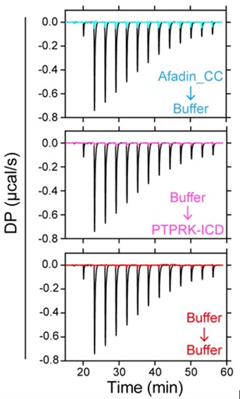
Author Response:
Reviewer #2 (Public Review):
There is now a considerable body of knowledge about the genetic and cellular mechanisms driving the growth, morphogenesis and differentiation of organs in experimental organisms such as mouse and zebrafish. However, much less is known about the corresponding processes in developing human organ systems. One powerful strategy to achieve this important goal is to use organoids derived from self-renewing, bona fide progenitor cells present in the fetal organ. The Rawlins' lab has pioneered the long-term culture of organoids derived from multipotent epithelial progenitors located in the distal tips of the early human lung. They have shown that clonal cell "lines" can be derived from the organoids and that they capable of not only long-term self-renewal but also limited differentiation in vitro or after grafting under the kidney capsule of mice. Here, they now report a strategy to efficiently test the function of genes in the embryonic human lung, regardless of whether the genes are actively transcribed in the progenitor cells. The strengths of the paper are that the authors describe a number of different protocols (work-flows), based on Crisper/Cas9 and homology directed repair, for making fluorescent reporter alleles (suitable for cell selection) and for inducible over-expression or knockout of specific genes. The so-called "Easytag" protocols and results are carefully described, with controls. The work will be of significant interest to scientists using organoids as models of many human organ systems, not just the lung. The weaknesses are that they authors do not show that their lines can undergo differentiation after genetic manipulation, and therefore do not provide proof of principle that they can determine the function in human lung development of genes known to control mouse lung epithelial differentiation. It would also be of general interest to know whether their methods based on homologous recombination are more accurate (fewer incorrect targeting events or off target effects) than methods recently described for organoid gene targeting using non homologous repair.
We thank Reviewer #2 for capturing the key advances of our toolbox for understanding gene function using a tissue organoid system and the constructive suggestions for the manuscript.
We agree with the Reviewer that it would strengthen the current manuscript if we could differentiate the genetically targeted organoids. Therefore, as a proof of concept, we have successfully differentiated the SOX9 reporter organoids into the alveolar lineage (New figure: Figure 2-figure supplement 1g, shown above). We have also tested the dual SMAD inhibition approach recently reported for basal cell differentiation (Miller et al., 2020). However, this has led to massive cell death even in WT organoids (data not shown). We reason that this might be because our organoids are ~8 pcw, whereas in the literature ~12 pcw organoids were used. We believe that efficient airway differentiation will take a long time to optimise for our organoids and is therefore beyond the scope of this manuscript.
In regard to the Easytag workflow in comparison with the recent CRISPR-HOT method using non-homologous end joining (Artegiani et al., 2020), we consider our approach as a complement to the CRISPR-HOT approach. This can be reflected in the following points: (1) The Organoid Easytag workflow allows precise N-terminal tagging of endogenous genes, exemplified by N-terminal tagging of ACTB. This is not possible using CRISPR-HOT as large pieces of plasmid DNA would disrupt the targeted gene; (2) The Organoid Easytag workflow is based on HDR and the efficient insertion sites for exogenous genes are within a ~30-bp window of the gRNA cleavage sites (Kwart et al., 2017), which gives more flexibility for choosing gRNAs compared with CRISPR-HOT tagging; (3) The Organoid Easytag workflow gives researchers more control of where and how the targeted sites can be modified, and offers a minimal change to the targeted genomic region, whereas CRISPR-HOT introduces large pieces of backbone plasmids, which potentially increases the risk of gene dysregulation. However, HDR requires cells to be at the G2/M phase of the cell cycle, therefore heavily relying on fast cycling cells to gain the most efficient targeting. CRISPR-HOT has the great advantage of not depending on a specific cell cycle stage and therefore being more efficient in slow cycling cells. With this said, we do believe that the efficiency would very much rely on the context, including the cell type used and locus targeted, as a recent report suggested targeting efficiency is influenced also by genomic context (Schep et al., 2021).
In summary, when N-terminal tagging, minimal changes and precise control of targeting is desired, Organoid Easytag is more favourable; whereas when targeting slowly cycling cells, CRISPR-HOT has its strength. Therefore, we consider these two methods as complementary approaches that will both be of benefit to organoid-based research. We have summarised this comparison into a simple table (New table: Figure 2-figure supplement 5f)

Figure 2-figure supplement 5(f). A comparison of Organoid Easytag and CRISPR-HOT methods (Artegiani et al., 2020).
Reviewer #3 (Public Review):
Sun et al have assembled, modified, and applied a series of existing gene editing tools to tissue-derived human fetal lung organoids in a workflow they have termed "Organoid Easytag". Using approaches that have previously been applied in iPSCs and other cell models in some cases including organoids, the authors demonstrate: 1) endogenous loci can be targeted with fluorochromes to generate reporter lines; 2) the same approach can be applied to genes not expressed at baseline in combination with an excisable, constitutively active promoter to simplify identification of targeted clones; 3) that a gene of interest could be knocked-out by replacing the coding sequence with a fluorescent reporter; 4) that knockdown or overexpression can be achieved via inducible CRISPR interference (CRISPRi) or activation (CRISPRa). In the case of CRISPRi, the authors alter existing technology to lessen unwanted leaky expression of dCas9-KRAB. While these tools have previously been applied in other models, their assembly and demonstrated application to tissue-derived organoids here could facilitate their use in tissue-derived organoids by other groups.
Limitations of the study include:
1) is demonstrated application of these technologies to a limited set of gene targets;
2) a lack of detail demonstrating the efficiency and/or kinetics of the approaches demonstrated.
While access to human fetal lung organoids is likely not available to many or most researchers, it is probable that the principles applied here could carry over to other organoid models.
We thank the Reviewer for accurately summarising the details of our manuscript and positive comments on its potential to facilitate tissue-derived organoid related research. We are very grateful for the Reviewer’s detailed and constructive comments to help strengthen our manuscript.
In regard to the limitations pointed out by Reviewer #3, we have systematically tested the kinetics of the inducible CRISPRi knockdown effect and its reversibility using CD71 and SOX2 (New figure: Figure 3-figure supplement 2). At the same time, we have generated SOX9 reporter human foetal intestinal organoids using the Easytag workflow to further demonstrate it can be applied to another organoid system. As suggested by Reviewer #3, we also attempted to implement the inducible CRISPRi system in HBECs. However, due to their sensitivity to lentiviral transduction, infected HBECs died shortly after transduction with gRNA lentivirus. We believe that further optimisation of DNA delivery approach is required for implementation of the inducible CRISPRi/CRISPRa systems in HBECs (perhaps nucleofection and PiggyBac-based vectors).
Author Response:
Reviewer #1:
After infection, new HIV-particles assemble at the host cell plasma membrane in a process that requires the viral protein Gag. Here, Inamdar et al. showed that a component of the host cell, the membrane curvature-inducing protein IRSp53, contributes to efficiently promote the formation of viral particles in synergy with the viral Gag protein.
In cells depleted of IRSp53, the formation of HIV-1 Gag viral-like particles (VLPs) was compromised. The authors showed in compelling electron micrographs that the formation of VLPs was arrested at about half stage of particle budding. Biochemical data (co-IPs and analysis of VLPs and HIV particle content), super-resolution nanoscopy (single molecule localization microscopy) data, and in vitro biophysics measurements (in GUVs), all seem to indicate a functional connection between Gag and the iBAR-domain containing protein IRSp53. The combination of the different techniques and approaches is a clear strength of this manuscript. However, to my opinion, the interpretation of some of the experimental data is somehow limited by the lack of some appropriate controls (that are lacking for different reasons, as the authors state in some parts of the text). These are:
1) Specificity of the IRSp53 siRNA. Although the authors showed that the siRNA used can deplete the expression of the protein (both endogenous and ectopic), they did not presented any rescue experiments of the phenotypes (or corroboration with different siRNA oligoes).
We have tried several different commercial and home-designed siRNA targeting IRSp53 from different companies (providing single siRNA and multiple siRNA mix): we have summarizing all in the Figure R1 (see below). One can see that indeed only 2 siRNA were effective in extinguishing IRSp53 gene: one from Invitrogen on endogenous IRSp53 and ectopic IRSp53-GFP and one from Dharmacon that was only effective on ectopic IRSp53-GFP, as revealed by Western Blot (Fig R1A). Furthermore, the specificity of the siRNA was challenge by testing siRNA IRSp53 on human IRSp53-GFP and on mouse I-BAR-GFP in HEK293T transfected cells and visualized by fluorescence microscopy. Results show in figure R1B that only siIRSp53 is able to extinguished human IRSp53-GFP and not mouse I- BAR-GFP. SiIRTKS and siCtrl are not extinguishing any of these genes. Overall these results confirm the specificity of IRSp53 siRNA-mediated knockdowns.
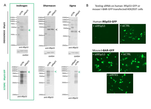
Figure R1: Specificity of siRNA-mediated knockdowns: (A) Western blots of HEK293T cells lysates probed with anti-IRSp53 antibody (and house-keeping gene GAPDH) showing a series of different siRNA IRSp53 (and siRNA Control, CTRL from Invitrogen, Dharmacon or Sigma) on endogenous and ectopic IRp53 genes in human HEK293T cells and their efficacy in specifically down regulating IRSp53. (B) siRNA IRSp53 from Invitrogen was tested for its specificity in extinguishing human IRSp53-GFP protein expressed in transfected HEK293T cells, but not mouse I-BAR-GFP, and as compare to siRNA control and IRTKS, revealed by fluorescence imaging (GFP).
To further answer the reviewers’ comments, we also perform one rescue experiment of the phenotype as shown in Figure R2 below. We observed that, upon co-transfection of pGag+pIRSp53- GFP+siRNA IRSp53 (lane 2), about 50% of the ectopic IRSp53-GFP was extinguished (since this construct is not siRNA resistant), leaving 50% of this ectopic protein expressed in the cells. In this context, one can observe that Gag-VLP release is ~50% (lane 2), similar to the condition pGag+siCTRL (lane 3). When we compare this to pGag+siIRSp53 (lane 4) which is reduced by 2-3 fold (data from Figure 1b of the manuscript), we can say that the remaining IRSp53-GFP in the Lane 2 seems to rescue the defect caused by extinction of the endogenous IRSp53. In the condition pGag+pIRSp53- GFP +siCTRL, VLP-Gag release was slightly reduced. This is an atypical rescue experiment since we do not have an IRSp53-GFP that is resistant to the siRNA IRSp53 used in this study (Figure R1B), but it suggests that if IRSp53-GFP is overexpressed in the presence of Gag and the siRNA IRSp53, VLP-Gag release is at a normal 50% level in contrast to the absence of IRSp53-GFP (compare lane 2 with lane 4). Unfortunately, due to limited time and by the siRNA IRSp53 out of stock, and the delay in supply, we could only provide one experiment. We thus decided to show it for answering the reviewers but not as part of a figure in the final manuscript.
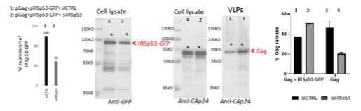
Figure R2: Rescue of siRNA IRSp53 knock-down with overexpression of IRSp53-GFP: 293T cell were transfected with pGag, pIRSp53 and siRNA control (siCTRL, lane 1) or siRNA IRSp53 (lane 2); cell lysat and VLP wre loaded on SDS-PAGE gels and immunoblots were revealed with anti-GFP (for IRSp53-GFP) and anti-CAp24 (for HIV-1 Gag). One graph on the left shows the percentage of IRSp53-GFP expression upon siRNA IRSp53 cell treatment (lane 2) as compare to the siRNA CTRL (lane 1). The graph on the right shows the resulting gel quantification for the % of Gag-VLP release upon siRNA IRSp53 cell treatment (lane 2) as compare to the siRNA CTRL (lane 1) in the presence of IRSp53-GFP over-expression, or without (lane 3 and 4, as in Figure 1b). N=1 rescue experiment.
2) In the co-IPs (IRSp53 IP + Gag co-IP) there is no assessment of the IRSp53 IP efficiency in the different conditions. The authors argued that IgG signal masking precluded them from doing that.
See the new figure 2. In the new figure 2b, we have assess the IP/co-IP of IRSp53-GFP/Gag efficiency by adding a complete experiment showing that an anti-GFP is able to pull down IRSp53- GFP very efficiently (lanes 2 and 3) and co-IP Gag efficiently (lane 3) accordingly to the input and remaining flowthrough. Using IRSp53-GFP and an anti-GFP antibody, we could bypass the IgG signal masking the endogenous IRSp53 with the IRSp53 antibody’s IP.
3) The authors observed an increase in the membrane-bound pool of IRSp53 when Gag is present (Fig. 2c). It is not clear whether this is specific for IRSp53 or other IBAR proteins can also be more membrane-bound as a result of Gag expression.
See the new figure 2. In the new figure 2d, we have re-loaded all the gel fractions on new SDS- PAGE gels and probed the corresponding immunoblots for Gag, IRSp53, IRTKS, Tsg101 and the cellular markers, Lamp2 (for membrane fractions) and ribosomal S6 protein (for cytosolic fractions). One can see that after quantification of the IRSp53 versus IRTKS bands in the HEK293T cell control and in the Gag expressing cells, only IRSp53 is increasing at the cell membranes upon Gag expression and not IRTKS.
Reviewer #3:
Inamdar et al. used biochemical and microscopy assays to investigate the role of I-BAR domain host proteins on HIV-1 assembly and release from HEK 293T and Jurkat cells. They show that siRNA knockdown of IRSp53, but not a similar I-BAR domain protein IRTKS, inhibits HIV-1 particle release from 293T cells after transfection of the HIV-1 provirus or HIV-1 Gag in cells. The authors then show that HIV-1 Gag associates with IRSp53 in the host cell membrane and cytoplasm, using biochemical assays and super resolution microscopy. In addition, IRSp53 is incorporated into HIV-1 particles along with other previously identified host proteins. Then using in vitro-derived membrane vesicles ("giant unilamellar vesicles" or GUVs), the authors indicate that HIV-1 Gag can associate with IRSp53, particularly on highly curved structures.
The conclusions are largely supported data, with the virology and biochemical results being particularly strong, but the mechanistic studies in GUVs appear somewhat preliminary and are not entirely clear. The GUV experiments would benefit from better quantification of measurements and manipulation to simulate actual cellular scenarios. In addition, while it is appreciated that the HEK 293T cell line is convenient for biochemical and imaging studies, they are not biologically relevant HIV-1 target cells. While the authors present examples of reproducibility of their results in a CD4+ T cell line, these data are buried in the supplemental figures, whilst it would have been better to highlight them and perhaps include primary CD4+ T cells.
1) Immortalized cell lines do not always recapitulate primary cells. It is unclear what the role of IRSp53 is in the membrane curvature of CD4+ T cells and whether expression levels and localization are consistent with Jurkat T cells.
Please consider the general responses to the Editors, which is:
We have published that IRSp53 (using siRNA) is involved in HIV-1 particle release on primary T cells (PBMC derived T cells) in Thomas et al, JVI 2015, so high probability is that it would be the same in different cell type, transfected HEK293T cells, transfected or infected Jurkat T cells and infected primary T cells. But we have not done the extensive super-resolution microscopy on infected primary T cells because this would require time overconsuming study. We are currently proceeding in setting up condition with an infectious HIV-1 virus carrying mEOS2 photoactivable protein for being able to infect primary T cells and go on for further research using infectious relevant system and super- resolution microscopy, but it is not ready for this current manuscript as it would require months of extra work and experiments.
Although, we agree with the reviewer #3 that the localization of Gag in Jurkat T cells and in primary CD4 Tc cells is different at the cell level (in primary T cells HIV-1 Gag is more polarized at uropods, as referred in the literature – see for an example Bedi et al/Ono’s Lab), but at the nanoscopic level of the budding sites, chances are that it would be similar but it need to be checked in future studies.
2) Description of some of the microscopy measurements could be improved. In lines 204-206 of the text and Figure S5, it is unclear how the localization of precision was determined to be approximately 16 nm for PALM-STORM.
These lines have been changed in the main text as they were not mandatory to understand how we determine the size of the VLP clusters. However, we have now detailed in figure S5 how we measure localisation precision.
The following text has been added to the legend of the figS5:
“Distribution of localisation precisions for PALM (in green) or STORM (in red) as given by Thunderstorm analysis in Fiji : Localisation precision distribution exhibit maxima at 16 nm and a mean±sd value of 20±5 nm for PALM, and a maxima of 26 nm, corresponding to a mean±sd value of 27±10 nm for STORM. The localization precision is obtained by eq 17 of (Thompson et al., 2002).”
As well as the reference of the original paper (Thompson et al. 2002, Biophysical Journal).
In Figure 4b, it is understood from the text (lines 252-256) that the red bars denote the Mander's coefficient for colocalization of the GFP-tagged proteins with Gag-mCherry (presumably the average of multiple experiments with standard deviations or errors of the mean, although this is not stated in the figure legend), it is unclear what the green bars are showing.
Yes, the red bars denote the Mander's coefficient for colocalization of the Gag-mCherry with the GFP-proteins, and the green bar denote for colocalization of the GFP-tagged proteins with Gag- mCherry, showing for more than 300 green and red vesicles, thant indeed all the Gag-VLP are green in the case of IRSp53-GFP (red bar) but that not all the GFP-IRSp53-GFP “green” vesicles are (+) for Gag: this indicates that vesicles produced by transfected HEK cells produced GAG/IRSp53 VLP but also IRSp53-GFP vesicles. Thanks to the reviewer to point this out. We added the explanation in the main text (page 12, lanes 272-282) and in the figure legend of Figure 4b.
Also, the histograms for IRSp53 and IRTKS colocalized with Gag look similar in Figure S10, suggesting that they are not different in Jurkat cells, but this is not addressed.
Yes. We have now addressed this particular point in the global response to the reviewers. Indeed, the figure 3 and 4 were remodelled into new figure 3 showing, in the same figure, HEK and Jurkat cells results and in figure 4 the simulations results. Overall, the PALM/STORM microscopy analysis results on Gag/IRSp53 colocalization are very similar in both cell types.
3) GUVs are first referenced on page 7 after description of Figure 2, the significance of which is confusing to the reader. However, the actual experimental data are described on pages 12-13 and Figures 5 and S11. A better description of these structures would be warranted for an audience that is unfamiliar with them. In addition, the biologic concentrations of I-BAR proteins at cell membranes are not provided and it is unclear what conditions used in Figures 5 and S11 represent a "normal CD4+ T cell" situation. It appears that the advantage of this in vitro system is that different factors can be provided or removed to simulate different cellular scenarios. For example, relatively low IRSp53 concentrations may simulate siRNA knockdown experiments in Figure 1, which could recapitulate those results that less viral particles are released from the membrane. In addition, the authors state that HIV-1 Gag preferentially colocalizes with IRSp53 as the tips of the GUV tubular structures (Figure 5b,c), but this is not actually shown or quantified. Similar quantification as shown in Figure 1e could be performed to strengthen this argument.
We thank the review for pointing this out. We now described all the GUV result in section 5.
Considering the biological concentrations of I-BAR proteins in cells, to the best of our knowledge, there is no measurement of it. We thus could not relate concentrations used in the GUV experiments with those in cells.
We could not perform quantification as in Figure 1e because the majority of the tubes in GUVs were moving too rapidly, preventing us from acquiring images with higher spatial resolution (see Fig. S11, and Movie 2 and 3). However, we would like to point out that the Gag signals appeared dotty inside GUVs (see Fig. S11, and Movie 2 and 3), which is very different from the signals of I-BAR that are clearly along the tubes (see Fig. S10c). Moreover, for tubes that were not moving too fast, we found that for all the tubes (17 tubes), Gag signals are exclusively located at the tips of the tubes (see new Fig. 6d). Also, the sorting maps shown in Fig. 6c and Fig. S10 d indicate the relative accumulations of Gag at the tips of the tubes. To make it clearer that the Gag signals were located at the tips of the tubes, in the current manuscript, we have added the new Fig. S11, Movie 1, 2 and 3, and included zoom-in images in Fig. 6b, 6c and a new Fig. 6d. Also, we have included the quantitation results (17 tubes) in the manuscript.
Author Response:
Reviewer #1 (Public Review):
The lateral entorhinal cortex (LEC) receives direct inputs from the olfactory bulb (OB) but their odor response properties have not been well characterized despite a recent increase in interests in the role of LEC in olfactory behaviors. In this study, Bitzenhofer and colleagues provide unprecedented details of odor response properties of layer 2 cells in LEC. The authors first show that LEC neurons respond to odors with a rapid burst of activity time-locked to inhalation onset, similarly to the piriform cortex (PCx), but distinct from the OB. Firing rates of LEC ensembles conveyed information about odor identify whereas timing of spikes odor intensity. The authors then examined the difference between two major cell types in LEC layer 2 - fan cells and pyramidal neurons, and found that, on average, fan cells responded earlier than pyramidal neurons, and pyramidal neurons, but not fan cells, changed their peak timing in response to changes in concentrations, providing a basis for temporal coding of odor concentrations. Additionally, the authors show that inactivation of LEC impairs odor discrimination based on either identify or intensity, and demonstrate different cellular properties of fan cells and pyramidal neurons. Finally, the authors also examined the odor response properties of hippocampal CA1 neurons, and showed that odor identify can be decoded by firing rate responses, while decoding of odor concentration depended on spike timing.
The authors performed a large amount of experiments, and provide an impressive set of data regarding odor response properties of LEC layer 2 neurons in a cell type specific manner. The results reported are very interesting, and will be a point of reference for future studies on odor coding and processing in the LEC. The manuscript is clearly written, and data are well analyzed and presented clearly. I have only relatively minor concerns or suggestions.
- The authors infer the time at which "mice could discriminate odors" from the time at which d-prime becomes significantly different between baseline and odor stimulation conditions (line 111 and line 121). However, the statistical test applied to these data does not guarantee that an observer can accurately discriminate odors. For example, a small p-value can be obtained even when discrimination accuracy is only slightly above chance if there are many trials. The statement such as "mice could discriminate two odors by as early as 225 ms after inhalation onset" (line 111) can be misleading because this might sound as if mice can accurately discriminate odors at this timepoint, while this is not necessarily the case (as indicated by the d-prime value).
We have added plots of performance accuracy over time under control conditions (LED off) to Figure 2-supplement 1. These plots of fraction of correct responses (binned every 50 ms) show that mice (n = 6) are making choices significantly different from chance within 200 ms of odor inhalation. We changed the wording in the Results to now say: “Moreover, by analyzing lick timing, we determined that the discriminability measure d’ became significantly different under control conditions as early as 225 ms after inhalation onset and performance accuracy increased within 200 ms of inhalation (Fig. 2b, Figure 2-supplement 1).”
- Optogenetic identification can be a little tricky when identifying excitatory neurons as in this study. Please discuss some rational or difficulty regarding how to distinguish those that are activated directly by light from those activated indirectly (i.e. synaptically). Do the results hold if the authors use only those that the authors are more confident about identification?
We only used the cells that were confidently identified using a combination of two criteria. First, tagged cells had to show a significant increase in firing (p_Rate <0.01) during the 5 ms LED illumination period versus 100 randomly selected time windows before LED stimulation. Cells also had to respond with a fixed latency to reduce the chance of including cells recruited by polysynaptic excitation. Further, we used the stimulus associated spike latency test (SALT) as detailed in Kvitsiani et al., 2013. To be judged as tagged, units had to show significantly less spike jitter during the 5 ms LED illumination than 100 randomly selected time windows before LED stimulation (p_SALT<0.01). Only those cells with BOTH p_Rate<0.01 and p_Salt<0.01 were considered as tagged (both methods typically agreed for most cells). Moreover, slice work testing synaptic connections between LEC layer 2 cells found extremely low levels of connectivity between fan and pyramidal cells Nilssen et al., J. Neuroscience, 2018. This makes it unlikely that LED-induced firing of fan or pyramidal cells would recruit indirectly (synaptically) excited cells.
- The authors sort odor response profiles by peak timing, and indicate that odor responses peak at different timing that tiles respiration cycles. However, this analysis does not indicate the reliability of peak timing. Sorting random activity by "peak timing" could generate similar figure. One way to show the reliability or significance of peaks is to cross-validate. For instance, one can use a half of the trials to sort, and plot the rest of the trials. If the peak timing is reliable, the original pattern will be replicated by the other half, and those neurons that are not reliable will lose their peaks. Please use such a method so that we can evaluate the reliability of peaks.
We analyzed the data as suggested by this reviewer as shown below (Author response image 1). Plotting only the odd trials sorted by the odd trials in the dataset (top) looked identical to the data from all trails used in Figure 1g. More importantly, plotting only the even trials sorted by the odd trials (bottom), though noisier due to trial-by-trial variation, showed the same general structure of tiling throughout the respiration cycle for OB cells.
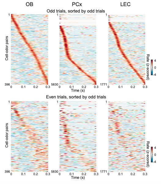
Author response image 1
Reviewer #2 (Public Review):
In this study, Bitzenhofer et al recorded odor-evoked activity in the LEC and examined the coding of odor identity and intensity using extracellular recordings in head-fixed mice, and used the standard suite of quantitative tools to interpret these data (decoding analyses, dimensionality reduction, etc). In addition, they performed behavioral experiments to show the necessity of LEC in odor identity and intensity discrimination, and deploy some elegant and straightforward 'circuit-busting' slice physiology experiments to characterize this circuit. Importantly, they performed some of their experiments in Ntng1-cre and Calb-cre mice, which allowed them to differentiate between the two major classes of LEC principal neurons, fan cells and pyramidal cells, respectively. Many of their results are contrasted with what has previously been observed in the piriform cortex (PCx), where odor coding has been studied much more extensively.
Their major conclusions are:
Cells in the LEC respond rapidly to odor stimuli. Within the first 300 ms after inhalation, odor identity is encoded by the ensemble of active neurons, while odor intensity (more specifically, responses to different concentrations) is encoded by the timing of the LEC response; specifically, the synchrony of the response. These coding strategies have been described in the PCx by Bolding & Franks. Bolding also found two populations of responses to different concentrations: one population of responses was rapid and barely changed with concentration and the second population of responses had onset latencies that decreased with increasing concentration. Roland et al also found two populations of responses using calcium imaging in anesthetized mice: one population of responses was concentration-dependent and another population was 'concentration-invariant'. However, neither Bolding nor Roland were able to determine whether these populations of responses emerged from distinct populations of cells. Here, the authors elegantly register these two response types in LEC to different cell types: fan cells respond early and stably, and pyramidal cells response latencies decrease with concentration. This is a novel and important finding. They also showed that, unlike PCx or LEC where concentration primarily affects timing rather than rate/number, odor concentration in CA1 is only reflected in the timing of responses.
Using optogenetic suppression of LEC in a 2AFC task, the authors purport to show that LEC is required for both the discrimination of odor identity and odor intensity. If true, this is an important result, but see below.
In slice experiments, the authors characterize the differential connectivity of fan and pyramidal cells to direct olfactory bulb input, input from PCx, and inhibitory inputs from SOM and PV cells. This work is elegant, novel, and important, although it is a little out of place in this manuscript. As such, their findings are irrelevant/orthogonal to the rest of the results in this study. But fine.
The simultaneous recordings from three different stations along the olfactory pathway are impressive.
Major concern
My major concern with this manuscript regards the behavioral experiments. The authors show that blue light over the LEC in GAD2-Cre/Ai32 mice completely abolishes (i.e. to chance) the mouse's ability to perform a 2AFC task discriminating between either two different odorants or one odorant at different concentrations. Their interpretation is that LEC is required for rapid odor-driven behavior. The sensory component of the task is so easy, and the effect is so striking that I find this result surprising and almost too good to be true. The authors do control for a blue-light distraction effect by repeating the experiments in mice that don't express ChR2, but do not control for the effect of rapidly shutting down a large part of the sensory/limbic system. If they did this experiment in the bulb I would be impressed with how clean the result was but not conceptually surprised by the outcome. I think a different negative control is needed here to convince me that the LEC is necessary for this simple sensory discrimination task. For example, the authors could activate all the interneurons (i.e. use this protocol) in another part of the brain, ideally in the olfactory pathway not immediately upstream of the LEC, and show that the behavior is not affected.
This reviewer suggests a negative control experiment for the effects we observe on behavior when optogenetically silencing LEC. However, we disagree that it would be informative to silence other olfactory pathways in search of those that do not affect behavior. Our strong effects on behavior are also in complete agreement with recent findings that muscimol inactivation of LEC abolishes discrimination of learned odor associations (Extended Data Figure 8, Lee et. al., Nature, 2021).
More specifically, both the presentation and the interpretation of the data are confusing. First, there is a lack of detail about the behavioral task. I was not sure exactly when the light comes on and goes off, when the cue was presented, and when the reward was presented. In the manuscript they say (line 108) "…used to suppress activity during odor delivery on a random subset…". There is nothing more about this in the figure legend or Methods. The only clue to this is the dotted line in the 'LED On' example at the bottom of Fig. 2a. The authors also say that (line 660) "Trials were initiated with a 50 ms tone." When exactly was the tone presented? In the absence of any other information, I assume it was presented at odor onset. When was the reward presented? Lines 106-7 say "Mice were free to report their choice (left or right lick) at any time within 2 s of odor onset." Presumably this means the reward was presented to one of the ports for 2 seconds, starting at odor onset.
The LED is applied during odor delivery, the 50 ms tone immediately precedes odor delivery, and water reward is dispensed after the first lick at the correct lick port during the choice period. The choice period begins with the odor onset and odor delivery is terminated by the first lick at either the correct or incorrect port. If there is no lick at either port, odor delivery lasts 1s and is followed by an extended choice period (terminated by correct or incorrect lick) lasting 1s. To clarify the behavior protocol, we have included a schematic of the trial structure in Figure 2-supplement 1.
These details matter because the authors want to claim that "LEC is essential for rapid odor-driven behavior." The data presented in support of this claim are (1) that mice perform this task at chance levels in LED On trials, presumably based on which port the mouse licked first (this is the 'essential' part), and (2) that in control in LED Off trials, d' becomes statistically different from baseline after ~200 ms (this is the 'rapid' part).
To further support the argument that LEC is required for rapid odor-driven behavior, we now show a plot of % correct responses over time from first odor inhalation.
On first reading, these suggested that shutting off LEC makes odor discrimination worse and/or slower. However, the supplementary data clarifies several things. First, the mice never Miss (Fig.2S.2a & c), meaning then they always lick. Second, in LED Off trials (F2S2 & e), the mice make few mistakes, and these only occur immediately after inhalation, presumably meaning the mice occasionally guess, possibly in response to the auditory cue. Thus, the mean time to lick is much shorter for Error trials than Correct trials. To state the obvious, the mice often wait >300 ms before they lick, and when they do wait, they never make mistakes. Now, in the LED On trials, the mice almost always lick within the first 300 ms and perform at chance levels, with the distribution of lick times for Correct and Error trials almost overlapping. In fact, although the authors claim LEC is required for rapid odor discrimination, the mean time to lick on Correct trials appears to decrease in LED On trials. This makes me think that the mice are making ballistic guesses in response to the tone in LED On cases, which doesn't necessarily implicate a dependence on LEC for odor discrimination.
We do not believe that mice are making ballistic guesses in response to the tone for LED on trials. First, although a 50 ms tone immediately precedes odor delivery, all data in Figure 2-supplement 1 shows lick times aligned to the first inhalation of odor. Thus, time 0 ms is not the tone or subsequent odor onset but rather a variable time point coinciding with the first odor inhalation (the delay from odor onset to first inhalation is ~300 ms, the average respiration interval under our conditions). In fact, we excluded trials if mice made premature licks between the time of odor onset and first odor inhalation. We re-analyzed these trials to test the reviewer’s idea that mice were more likely to make fast ballistic guesses when the LEC was silenced. However, we saw no evidence that mice made more premature licks in trials with LED on (Author response image 2).
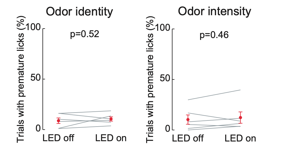
Author response image 2
The authors' interpretation of their data would be more solid if, for example, there were a delay between the auditory cue and odor delivery and/or if the reward was only available with some delay after the odor offset. Here, however, it seems just as likely as not that the mice are making ballistic guesses in response to the tone in LED On cases, which doesn't necessarily involve dependence on LEC for odor discrimination. Here, the divergence of d' from baseline in the control (i.e LED Off) condition seems mostly because mice take longer to correctly discriminate under control conditions. While this is not formally contradictory to LEC is essential for rapid odor-driven behavior", it is nevertheless a bit contrived and misleading. An interesting (thought) experiment is what would happen if the authors presented a tone but no odor. I would guess that the mice would continue licking randomly in Light On trials.
While a delay between odor delivery and reward would have been useful for some aspects of interpreting the behavior, we would have lost the ability to examine the role of LEC in response timing. To address this reviewer’s concern, we have added a section to the Discussion mentioning caveats related to the interpretation of experiments using acute optogenetic silencing to understand behavior.
Author Response
Reviewer #1 (Public Review):
We thank the reviewer for carefully reading of the manuscript and for the insightful criticisms and comments. In the following we address them point by point.
The community assembly process is modelled in a very specific way, and the manuscript would benefit from an expanded ecological motivation of the processes that are being mimicked, and thereby explain more clearly what taxonomic level of organization is being considered.
We follow the more recent trait-based approach that shifts the focus from species (and the many traits by which they differ from one another) to groups of species that share the same values of selected functional traits. Since the general context is ecosystem response to drier climates, we choose the functional traits to include a response trait associated with stress tolerance and an effect trait associated with biomass production. We further assume a tradeoff between the two traits which is well supported by earlier studies (see e.g. Angert et al. 2009, https://doi.org/10.1073/pnas.0904512106). So, indeed, the choice we make in characterizing the community is quite specific, but it is highly relevant to the ecological context considered of dryland plant communities where plants compete primarily for water and light. The taxonomic level we consider is species except that we group them in a manner that is more transparent to questions of ecosystem function, ignoring differences between species that are not significant to these questions.
We expanded considerably the text in the section “Modeling spatial assembly of dryland plant communities” to clarify the ecological motivation of the processes we model.
In addition, it would be useful if the authors could provide further clarification as to what extent the community diversity dynamics can be separated from total biomass dynamics of patterned water-limited ecosystems given the current approach. These points are explained in further detail below.
The model describes the dynamics of all functional groups, which provides the biomass distribution 𝐵 = 𝐵(𝜒) in trait space (in the case of patterned states we first integrate over space). That distribution contains information about various community-level properties, including functional diversity (richness, evenness) as figure 3 in the revised manuscript illustrates, and total biomass, which is the area below the distribution curve. The two types of dynamics are tightly connected and cannot be separated, but in principle the approach can be used to study the relationships between diversity and total biomass by calculating biomass distributions along the rainfall gradient and extracting the two properties from the distributions.
We added in the section “Modeling spatial assembly of dryland plant communities” the information that the biomass distribution also contains information about the total biomass.
First, it was not entirely clear to this reviewer how the reaction parts of the model equations determine the optimal trait value χ, and how this value varies as a function of precipitation.
The ‘optimal’ trait value 𝜒𝑚𝑎𝑥 is determined by the interspecific interactions that the model captures, which divide into ‘direct’ and ‘indirect’ interactions. The direct interactions are captured by the dependence of the growth rate Λ𝑖 of the ith functional group (see Eq. (1a)) on the aboveground biomass values of all functional groups, Λ𝑖 = Λ𝑖(𝐵1,𝐵2,… , 𝐵𝑁) (see Eq. (2)). This dependence represents competition for light (taller plants are better competitors) and includes the effect of self-shading. The indirect interactions are through the water uptake term in the soil-water equation (1b) (2nd term from right) and the water dependence of the biomass growth term in Eq. (1a). These terms represent competition for water. For a given precipitation value 𝑃 the net effect of these interspecific interactions result in a particular functional group 𝜒𝑚𝑎𝑥 which is most abundant. For spatially uniform vegetation, as 𝑃 is increased 𝜒𝑚𝑎𝑥 moves to lower values. The precipitation increases surface water (Eq. (1c)) and consequently the amount of water 𝐼𝐻 infiltrating into the soil. The increased soil water gives competitive advantage to species investing in growth, mainly because they better compete for light as they grow taller, and therefore 𝜒𝑚𝑎𝑥 decreases.
… it is then not immediately clear why the most successful trait class is not outcompeting the other classes.
With the current model and parameters set the most successful trait does eventually outcompete all other traits, when trait diffusion is set to zero, 𝐷𝜒 = 0. This is, however, a very long process because the most successful trait suffers from self-shading at late growth stages, which slows down its growth and allows nearby traits to survive for a long time. Choosing a finite but very small 𝐷𝜒 values that represent mutations occurring on evolutionarily long times counteracts the exclusion process and results in a stationary asymptotic community, as Fig. 3 in the revised manuscript shows (this behavior is reminiscent of optical solitons, where self-focusing instability is balanced by dispersion). We note that modeling stronger growth-inhibiting factors, such as pathogens, by including a factor of the form (1 − 𝐵𝑖/𝐾) to the growth rate, results in an asymptotic stationary community also for 𝐷𝜒 = 0 (see also earlier studies Nathan et al. 2016, Yizhaq et al. 2020).
We revised original Fig. 4 (now Fig. 3) by adding a new part (Fig. 3a) that shows the exclusion process for 𝐷𝜒 = 0, and the effect of the counter-acting process of trait diffusion, which results in an asymptotic distribution of finite width (Fig. 3b) from which community level properties such as functional diversity can be derived. We also extended the text in section “Modeling spatial assembly of dryland plant communities” (last paragraph) to clarify the two counter-acting processes of exclusion because of interspecific competition for water and light, and trait diffusion driven by mutations, which together culminate in an asymptotic biomass distribution along the 𝜒 axis of finite width.
The authors model trait adaptation through a diffusion approximation between trait classes. That is, every timestep, a small amount of biomass flows from the class with higher biomass to the neighboring trait class with lower biomass. From an ecological point of view, it seems that this process is describing adaptation of vegetation that is already present, so this process seems to be limited to intraspecific phenotypic plasticity. From the text, however, it seems that the trait classes correspond to higher taxonomic levels of organization, when describing shifts from fast growing to stress-tolerant species, for example. It is not entirely clear, however, how biomass flows as assumed in the model could occur at these higher levels of organization.
We do not study in this work adaptation through diffusion in trait space. That kind of adaptive dynamics can indeed be studied with the current model, but with different initial conditions, namely, initial conditions corresponding to a single resident trait where the biomass of all other traits is zero. The resulting dynamics of mutations and succession are then very slow, occurring on evolutionarily long time scales set by the small value of 𝐷𝜒 (e.g. 10−6). In this study the initial conditions represent the presence of all traits, even if at very low biomass values that may represent a pool of seeds that germinate once environmental conditions allow. For a given precipitation value 𝑃, the functional traits we consider determine which functional groups (of species) overcome environmental filtering and grow, and which of the growing traits survive the competition for water and light. These are relatively fast processes, occurring on ecological time scales, which determine the emerging community. At longer times this community is further shaped by slow processes of interspecific competition among species of similar traits and by trait diffusion (mutations). A final remark about phenotypic changes: although in general 𝜒 can be interpreted as representing different phenotypes, the choice of very small values for 𝐷𝜒 cannot represent relatively fast phenotypic changes and restricts the context to mutations at the taxonomic level of species.
We added an explanation in the 3rd paragraph of the section “Modeling spatial assembly of dryland plant communities” of the need to consider mutations and the role they play in our study.
Combining the observations from the previous two points, there is a concern that for a given level of precipitation, there is a single trait class with optimal biomass/lowest soil water level that is dominant, with the neighboring trait classes being sustained by the diffusion of biomass from the optimal class to neighboring inferior classes. This would seem a bit problematic, as it would mean that most classes are not a true fit for the environment, and only persist due to the continuous inflow of biomass. Taking a clue from the previous papers of the authors, it seems this may not be the case, though. Specifically, in the paper by Nathan et al. (2016) it seems that all trait classes are started at low initial biomass density, and the resulting steady state (in the absence of biomass flows between classes) seems to show similar biomass profiles as shown in Figs. 4,5 and 7 of the current paper. While the current model formulation seems slightly different, similar results may apply here. Indeed, keeping all trait classes at non-zero (but low) density, and when the (abiotic and biotic) environment permits, let each class increase in biomass seems like the most straightforward approach to model community assembly dynamics. Given the above discussion about these trait classes competing for a single resource (soil water), and one trait class being able to drive this resource availability to the lowest level, it would then be useful to readers to explain why multiple trait classes can coexist here, and how(for spatial uniform solutions) the equilibrium soil water level with multiple trait classes present compares to the equilibrium soil water level when only the optimal trait class is present. Furthermore, if results as presented in Nathan et al. (2016) indeed hold in the current case, perhaps it means that the biomass profile responses as shown in e.g. Fig. 5 would also occur if there was no biomass flow between trait classes included, but that the time needed to adjust the profile would take much longer as compared to when the drift term/second trait derivative is included. In summary, further clarification of what the biomass flows between classes represent, and the role it plays in driving the presented results would be useful for readers.
As explained in the reply to previous comments the asymptotic community is tuned by a balance between two slow counter-acting processes, interspecific competition among similar traits and mutations over evolutionarily long time scales. However, the community structure is largely determined by much faster processes of environmental filtering and interspecific competition among widely distinct traits, as all traits are initially present. Indeed, comparing the biomass distributions in new Fig. 3, with and without trait diffusion indicates that the community composition, as measured by 𝜒𝑚𝑎𝑥, is the same. Trait diffusion, however, does affect functional diversity, along with environmental factors. In that sense the emerging community is a true fit for the environment.
We thank the reviewer for these thoughtful comments, which helped us realize that our presentation of these issues was too concise and unclear. We believe that the new extended section on modeling spatial assembly of dryland plant communities, and the new figure 3a clarify these issues.
In addition, it would be useful for readers to understand to what extent the shifts in average trait values and functional diversity can be decoupled from the biomass and soil water responses to changes in precipitation that would occur in a model with only a single biomass variable. For example, early studies on self-organization in semi-arid ecosystems already showed that the shift toward a patterned state involved the formation of patches with higher biomass, and higher soil water availability, as compared to the preceding spatially uniform state, and that the biomass in these patches remains relatively stable under decreasing rainfall, while their geometry changes (e.g. Rietkerket al. 2002). It has also been observed that for a given environmental condition, biomass in vegetation patches tends to increase with pattern wavelength (e.g. Bastiaansen and Doelman 2018; Bastiaansen et al. 2018). Given the model formulation, one wonders whether higher biomass in the single variable model is not automatically corresponding to higher abundance of faster growing species and a higher functional diversity (as the diffusion of biomass can cover a broader range when starting from higher mass in the optimal trait class). There are some indications in the current work that the linkage is more complicated, for example, the biomass peak in Fig. 7c is lower, but also broader as compared to the distribution of Fig. 7b, but it is currently not entirely clear how this result can be explained (for example, it might be the case that in the spatially patterned states, the biomass profiles also vary in space).
We are not sure we understand what the reviewer means by “decoupled”, but much insight indeed can be gained from a study of a model for a single functional group (trait) and observing the behaviors described by the reviewer. In fact, these behaviors, which some of us are familiar with from numerical studies, motivated parts of the current study. Higher biomass in vegetation patches (compared to uniform vegetation) in the single trait model does not automatically imply a shift to faster growing species; in principle the stress-tolerant species that already reside in the system when uniform vegetation destabilizes to a periodic pattern can simply grow denser. To answer this and additional questions we need to take into account interspecific interactions by studying the full community model. As to Fig. 7b,c, the behavior appears to be opposite to that described by the reviewer: the biomass pick in Fig. 7c is higher and narrower than that in Fig. 7b, not lower and broader. This is because of the much larger domain of the patterned state as compared with that of the uniform state, which increases the abundance of low-𝜒 species, i.e. species investing in growth.
The increase of biomass in vegetation patches with pattern wavelength for given environmental conditions, as observed by Bastiaansen et al. 2018, is actually another mechanism for increasing functional diversity. This is because the water stress at the patch center is higher than that in the outer patch areas and thus forms favorable conditions for stress tolerant species while the outer areas form favorable conditions for fast growing species.
We added a new paragraph in the Discussion and Conclusion section (last paragraph in the subsection Insight III) where we discuss the effect of coexisting periodic patterns of different wavelengths on functional diversity and ecosystem management. We also added citations to the references the reviewer mentioned.
The possibility of hybrid states, where part of the landscape is in a spatially uniform state, while the other part of the landscape is in a patterned state, is quite interesting. To better understand how such states could be leveraged in management strategies, it would be useful if a bit more information could be provided on how these hybrid states emerge, and whether one can anticipate whether a perturbation will grow until a fully patterned state, or whether the expansion will halt at some point, yielding the hybrid state. It seems that being able to distinguish this case would be necessary in the design of planning and management strategies
The hybrid states appear in the bistability range of the uniform and patterned vegetation states, and typically occupy most of this range. Their appearance is related to the behavior of ‘front pinning’ in bistability ranges of uniform and patterned states in general. Front pinning refers to fronts that separate a uniform domain and a periodic-pattern domain, which remain stationary in a range of a control parameter (precipitation in our case). This is unlike fronts that separate two uniform states, which always propagate in one direction or another and can be stationary only at a single parameter value – the Maxwell point. Thus, an indication that a given landscape may have the whole multitude of hybrid states is the presence of a front (ecotones) that separates uniform and patterned vegetation. If that front appears stationary over long period of times (on average), this is a strong indication.
We added a new paragraph in the subsection Insight III of the Discussion and conclusion section to clarify this point.
Also, in Fig. 3a, the region of parameter space in which hybrid states occur is not very large; it is not entirely clear whether the full range of hybrid states is left out here for visual considerations, or whether these states only occur within this narrow range in the vicinity of the Turing instability point.
As pointed out in the reply to the previous comment the hybrid states are limited to the bistability range of uniform and patterned vegetation, which is not wide. However, this should not necessarily restrictma nagement of ecosystem services by nonuniform biomass removal, as such management will have similar effects on community structure also outside the bistability range where front propagate slowly.
The new paragraph we added also addresses this point.
Reviewer #2 (Public Review):
We thank the reviewer for carefully reading the manuscript and for the constructive criticisms and comments. In the following we address them point by point.
1) Model presentation.
It would be better to explain the model in ecological terms first, clarifying parameter biological meaning and justifying their choice. In doing so, creating a specific 'Methods' section, which now is lacking, would be of help too. Authors should clarify whether and how the model follows the conservation of mass principle involving precipitation and evapotranspiration. Are root growth and seed dispersal included for this purpose? Why they are not referred to any further in the analysis and discussion? Why a specific term for plant transpiration is not included, or is to somehow phenomenologically incorporated into the growth-tolerance tradeoff? In doing so, authors should also pay attention to water balance as above (H) and below (W) ground water are not independent from each other.
We added a Methods section, which in eLife is placed at the end of the manuscript. The section includes the model equations and more detailed explanations in ecological terms of various parts of the model. We also added Table 1 with a list of all model parameters, their descriptions, units and numerical values used in the simulations. Presenting the model at the end of the manuscript suits more technical information about the model, but not essential information that is needed for understanding the results. We therefore kept the subsection “A model for spatial assembly of dryland plant communities” in the Results section, where we present that information.
There is no conservation of mass in the model (and all other models of this kind) simply because the system that we consider is open. In particular, it does not include the atmosphere, which constitute part of the system’s environment. Including the atmosphere as additional state variables in the model, capturing the feedback of evapotranspiration on the atmosphere, would make the model too complicated for the kind of analysis we perform. So, although the model contains parts that represent mass conservation such as the terms describing below- and above-ground water transport, water mass is not conserved. The biomass variables represent aboveground biomass of living plants or plant parts and are not conserved either as biomass production involve biochemical reactions that convert inorganic substances coming from the system’s environment (atmosphere and the soil) into organic ones, while plant mortality involves organic matter that leaves the system.
Roots in the model platform we consider are modeled indirectly through their relation to aboveground biomass. That relation constitutes one of the scale-dependent feedbacks that produce a Turing instability to vegetation patterns, the so-called root-augmentation feedback (see Meron 2019, Physics Today), but in this particular study we eliminate this feedback for simplicity. The scale-dependent feedback that we do consider is the so-called infiltration feedback, associated with biomass-dependent infiltration rate that produces overland water flow towards vegetation patches, as explained in the subsection “A model for spatial assembly of dryland plant communities”. It will be interesting indeed to extend the study in the future to include also the root-augmentation feedback.
We assume short-range seed dispersal and take it into account through biomass “diffusion” terms (obtained as approximations of dispersal kernels assuming narrow kernels). These terms play important roles in the scale-dependent feedback that induces the Turing instability, as is explained in earlier papers which we cite. Plant transpiration is modeled through the water uptake term in the equation for the soilwater 𝑊. Indeed above-ground water 𝐻 and below-ground water 𝑊 are not independent; the infiltration term IH in the equations for both state variables account for this dependence in a unidirectional manner (loss of 𝐻 and gain of 𝑊). As we do not include the atmosphere in the model the other direction, namely, evapotranspiration that increases air humidity and affects rainfall, is not accounted for. The neglect of this effect can be justified for sparse dryland vegetation.
These good points have already been discussed in many earlier papers as well as in the book Nonlinear Physics of Ecosystems (Meron 2015), and we cannot address them all in this paper. We did however add several clarifications in the section Modeling spatial assembly of dryland plant communities and in the new Methods section, including the consideration of the atmosphere as the system’s environment quantified by the precipitation parameter 𝑃.
Another unclear point is that growth rates for the same plant functional groups are assumed to be constant among different species within the same group and are confounded by biomass production. Why is that the case? Furthermore, how many different species are characterizing each functional group? How are interspecific interactions accounted for (more specifically, see comment below)?
In the trait-based approach we focus on just two functional traits, related to growth rate and tolerance to water stress, ignoring differences in other traits that distinguish species. That is, a given functional group consists of species that share the same values of the two selected functional traits (to a given precision determined by 𝑁), taking all other traits represented in the model to be equal. In this approach we do not care about how many species belong to each functional group, only their total biomass. We wish to add that simplifying assumptions of this kind are necessary if we want the model to be mathematically tractable and capable of providing deep insights by mathematical analysis.
We expanded the discussion of the trait-based approach in the section Modeling spatial assembly of dryland plant communities and added relevant references (second paragraph).
Finally, stress tolerance is purely phenomenological. There is no actual mechanism/parameter describing it. Rather, it "simply" appears as low/high mortality, which in turn is said to be due to high/low tolerance. This leads to a sort of circularity between mortality and tolerance. Yet, mortality can occur due to other biophysical factors (e.g. disturbance, fire, herbivory, pathogens). A drawback of this assumption is that a mechanism of drought tolerance is often to invest in belowground organs, including roots. However, according to the proposed model, it turns out that fast growing species with low investment in tolerance also have high investment in roots; vice versa, tolerant species have low investment in roots. This is a bit counterintuitive and not well biologically supported.
First, we agree with the reviewer that our approach is purely phenomenological, as we model tolerance to water stress by a single parameter that lumps together the effects of various physiological mechanisms. That parameter can be distinguished from other factors affecting mortality by regarding the constant 𝑀𝑚𝑎𝑥 in Eq. (3) as representing several contributions. Since we do not study the effects of these other factors we can absorb them in 𝑀𝑚𝑎𝑥 for mathematical simplicity. Tolerance to water stress is not necessarily associated with roots. Plants can better tolerate water stress by reducing transpiration through stomatal closure, regulating leaf water potential, or develop hydraulically independent multiple stems that lead to a redundancy of independent conduits and higher resistance to drought (see Schenk et al. 2008 - https://doi.org/10.1073/pnas.0804294105).
We added a discussion in the Methods section (5th paragraph, “Tolerance to water stess …”) of the simple form by which we model tolerance to water stress through the mortality parameter.
2) Parameter choice.
N = 128 is an extremely high number for plant functional groups. It is even quite unrealistic to have 128 species per square meter, so this value is not very reasonable. Please run the model and report results with more realistic N (e.g from 4-64) as well as with different sets of N values keeping all other parameters constant.
We wish to clarify two points: 1) N=128 does not imply 128 functional groups per square meter; the emerging community has much lower functional richness (FR) as the average FR is around 0.25, meaning only 128 × 0.25 = 32 functional groups. 2) The model results, as reflected by the key metrics 𝜒𝑚𝑎𝑥, 𝐹𝑅, and 𝐹𝐸, are independent of the particular value of N (for N values sufficiently large), as Figures IA and IB below show. The biomass 𝐵𝑖 of each functional group, however, does change (Figure IA) because by changing N we change the range of traits Δ𝜒 = 1/𝑁 that belong to a given functional group. But if we look at the biomass density in trait space 𝑏𝑖, related to 𝐵𝑖 through the relation 𝐵𝑖 = 𝑏𝑖Δ𝜒, then also the biomass density is independent of 𝑁 as Figure IB shows. So, even if in practice there are less functional groups and thus species as considered in the model studies, the results are not affected by that. On the other hand, choosing higher 𝑁 values provides smoother curves and nicer presentation of our results.
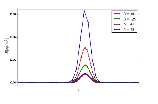
Figure IA
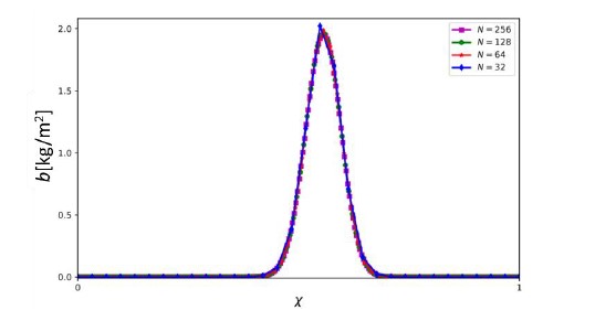
Figure IB
We added a discussion of this issue in the Methods section after Eq. (2).
Gamma (rate of water uptake by plants' roots): why is it in that unit of m^2/kg * y? Why are you now considering the area (and not the volume) per biomass unit?
The vegetation pattern formation model we study, like most other models of this kind, does not explicitly capture the soil depth dimension. Accordingly, W is interpreted as the soil-water content in the soil volume below a unit ground area within the reach of the plant roots. In practice W has units kg/m2, like B, and since Γ𝑊𝐵 should have the same units as 𝜕𝑊/𝜕𝑡 (see Eq. 1b), Γ must have the units of (𝐵𝑡)−1.
A is not defined in the text.
We now define it in Table 1 (see Methods section).
M min: why 0.5 mortality? Having M max set to 0.9, please consider a lower mortality value set to 0.1, and please report evidence(hopefully) demonstrating the robustness of results to such change.
The results are robust to the particular values of 𝑀𝑚𝑖𝑛 and 𝑀𝑚𝑎𝑥, except that there are combinations of these two parameters for which the biomass distributions are pushed towards the edge of the 𝜒 domain, which make the presentation of the results less clear. Figure II shows results of recalculations of the distribution 𝐵 = 𝐵(𝜒) for 𝑀𝑚𝑖𝑛 = 0.1, as requested (using 𝑀𝑚𝑎𝑥 = 0.15) for 3 different precipitation values. As the reviewer can see there’s no qualitative change in the results: lower precipitation push a uniform community to stress tolerant species (higher 𝜒), while the formation of patterns at yet lower precipitation push the community back to fast growing species (low 𝜒).
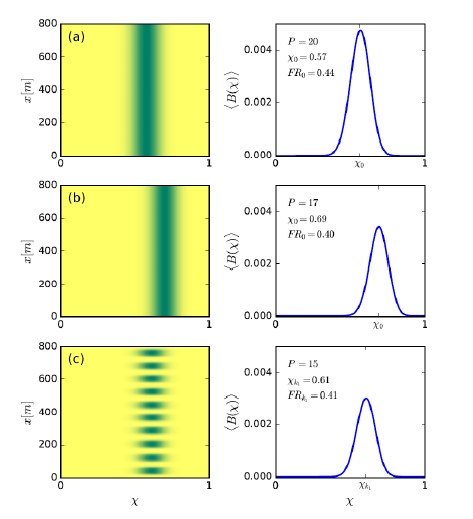
Figure II
K_min and K_max are in two different units, and should both be kg/m^2.
Thanks, we fixed this typo in Table 1.
Values of precipitation (P, mean annual precipitation) are not reported.
The precipitation parameter is variable, as is now stated in Table 1, and therefore was not include it in the list of parameters’ values used. Whenever a particular precipitation value has been used our intention was to state it in the caption of the corresponding figure. This was done in Figs. 5,6,7, but indeed not in Fig. 4 (Fig. 3 in revised ms.). The insets on the right side of Fig. 3 (Fig. 4 in revised ms.) where also calculated for particular precipitation values, but that information is not essential as the intention is to show typical forms of the various solution branches, which do not qualitatively change along the branches (i.e. at different P values).
We added the precipitation value (P=180mm/y) at which all the biomass distributions shown in new Fig. 3 (Fig. 4 in original ms) were calculated.
3) Results presentation and interpretation.
Parameter range of precipitation in figure 3 is odd. Why in one case precipitation ranges from 0 to 160 while in another it is only 60-120? Furthermore, in paragraph 198-213 and associated results in fig. 5. the Choice of precipitation values is somehow discordant from the previous model. Please provide motivation for this choice, clarify and uniformize it.
In Fig. 3b (Fig. 4b in revised ms) we restricted the precipitation range to 60-120 as the curves, which are limited to 0 < 𝜒 < 1 (by the definition of 𝜒), do not extend to 𝑃 < 60 and to 𝑃 > 120. Extending the range to 0 < 𝑃 < 160 would make the figure less compact and nice as it will contain blank parts with no information.
We are not sure we understand what the reviewer means by “is somehow discordant from the previous model”. The motivation of the choices we made for the precipitation values P=150, 100 and 80 was to show the shift of a spatially uniform community to a higher 𝜒 value as the precipitation is decreased to a lower value (from 150 to 100), and the shift back to a lower 𝜒 value at yet lower precipitation (80) past the Turing instability.
Finally, authors seem to create confusion around community composition, which is defined as the (taxonomic) identity of all different species inhabiting a community. Notably, it is remarkably different from the x_max parameter used in the model, which as a matter of fact is just the value of the most productive (notably, not necessarily the most abundant) functional group.
We thank the reviewer for this comment. Since all the emerging communities in the model studies are pretty localized around the value of 𝜒𝑚𝑎𝑥, that value does contain information about the identity of other functional groups in the community when complemented by FR (functional richness) and FE (functional evenness). More significantly to our study, shifts in 𝜒𝑚𝑎𝑥 represent the shifts in community composition we focus on in this study, i.e. shifts towards fast growing species or towards stress-tolerant species.
We modified the description of the community-level properties that can be derived from the biomass distribution in trait space (see modified text towards the end of the section “Modeling spatial assembly …” and also the caption of Fig. 3b), explaining that both functional diversity and community composition can be described by several metrics, and clarifying the significance of 𝜒𝑚𝑎𝑥 in describing community-composition shifts.
Author Response
Reviewer #1 (Public Review):
The authors convincingly show in this study the effects of the fas5 gene on changes in the CHC profile and the importance of these changes toward sexual attractiveness.
The main strength of this study lies in its holistic approach (from genes to behaviour) showing a full and convincing picture of the stated conclusions. The authors succeeded in putting a very interdisciplinary set of experiments together to support the main claims of this manuscript.
We appreciate the kind comments from the reviewer.
The main weakness stems from the lack of transparency behind the statistical analyses conducted in the study. Detailed statistical results are never mentioned in the text, nor is it always clear what was compared to what. I also believe that some tests that were conducted are not adequate for the given data. I am therefore unable to properly assess the significance of the results from the presented information. Nevertheless, the graphical representations are convincing enough for me to believe that a revision of the statistics would not significantly affect the main conclusions of this manuscript.
We apologize for neglecting a detailed description of statistical tests that were performed. We wrote additional paragraphs in the method part specifically explaining the statistical analyses (line 435-445; 489-502; 559-561; 586-591).
The second major problem I had with the study was how it brushes over the somewhat contradicting results they found in males (Fig S2). These are only mentioned twice in the main text and in both cases as being "similarly affected", even though their own stats seem to indicate otherwise for many of the analysed compound groups. This also should affect the main conclusion concerning the effects of fas5 genes in the discussion, a more careful wording when interpreting the results is therefore necessary.
Thank you for pointing this out. Though our focus clearly lay on the female CHC profiles as a function in sexual signaling has only been described thus far for them, we now elaborated the result and discussion for the fas5 RNAi male part (line 167-178; 258-268).
Reviewer #2 (Public Review):
Insects have long been known to use cuticular hydrocarbons for communication. While the general pathways for hydrocarbon synthesis have been worked out, their specificity and in particular the specificity of the different enzymes involved is surprisingly little understood. Here, the authors convincingly demonstrate that a single fatty acid synthase gene is responsible for a shift in the positions of methyl groups across the entire alkane spectrum of a wasp, and that the wasps males recognize females specifically based on these methyl group positions. The strength of the study is the combination of gene expression manipulations with behavioural observations evaluating the effect of the associated changes in the cuticular hydrocarbon profiles. The authors make sure that the behavioural effect is indeed due to the chemical changes by not only testing life animals, but also dead animals and corpses with manipulated cuticular hydrocarbons.
I find the evidence that the hydrocarbon changes do not affect survival and desiccation resistance less convincing (due to the limited set of conditions and relatively small sample size), but the data presented are certainly congruent with the idea that the methyl alkane changes do not have large effects on desiccation.
We appreciate the kind comments from the reviewer.
Reviewer #3 (Public Review):
In this manuscript, the authors are aiming to demonstrate that a fatty-acyl synthase gene (fas5) is involved in the composition of the blend of surface hydrocarbons of a parasitoid wasp and that it affects the sexual attractiveness of females for males. Overall, the manuscript reads very well, it is very streamlined, and the authors' claims are mostly supported by their experiments and observations.
We appreciate the kind comments from the reviewer.
However, I find that some experiments, information and/or discussion are absent to assess how the effects they observe are, at least in part, not due to other factors than fas5 and the methyl-branched (MB) alkanes. I'm also wondering if what the authors observe is only a change in the sexual attractiveness of females and not related to species recognition as well.
We appreciate the interesting point that the reviewer raises in sexual attractiveness and species recognition and now expand upon this potential aspect in the discussion (lines 327-330). However, in this manuscript, we very much focused on the effect of fas5 knockdown on the conveyance of female sexual attractiveness in a single species (Nasonia vitripennis). Therefore, we argue that species recognition constitutes a different communication modality here, and we currently cannot infer whether and how species recognition is exactly encoded in Nasonia CHC profiles despite some circumstantial evidence for species-specificity (Buellesbach et al. 2013; Mair et al. 2017). Thus, we would like to refrain from any further speculation on species recognition before this can be unambiguously demonstrated, and remain within the mechanism of sexual attractiveness within a single species which we clearly show is mediated by the female MB-alkane fraction governed by the fatty acid synthase genes. We however still consider potential alternative explanations (e.g., n-alkenes acting as a deterrent of homosexual mating attempts).
The authors explore the function of cuticular hydrocarbons (CHCs) and a fatty-acyl synthase in Nasonia vitripennis, a parasitic wasp. Using RNAi, they successfully knockdown the expression of the fas5 gene in wasps. The authors do not justify their choice of fatty-acyl synthase candidate gene. It would have been interesting to know if that is one of many genes they studied or if there was some evidence that drove them to focus their interest in fas5.
In a previous study, 5 fas candidate genes orthologous to Drosophila melanogaster fas genes were identified and mapped in the genome of Nasonia vitripennis (Buellesbach et al. 2022). We actually investigated the effects of all of these fas genes on CHC variation, but only fas5 led to such a striking, traceable pattern shift. We are currently preparing another manuscript discussing the effects of the other fas genes, but decided to focus exclusively on fas5 here, due to its significance for revealing how sexual attractiveness can be encoded and conveyed in complex chemical profiles, maintained and governed by a surprisingly simple genetic basis.
The authors observe large changes in the cuticular hydrocarbons (CHC) profile of male and females. These changes are mostly a reduction of some MB alkanes and an increase in others as well as an increase of n-alkene in fas5 knockdown females. For males fas5 knockdowns, the overall quantity of CHC is increased and consequently, multiple types of compounds are increased compared to wild-type, with only one compound appearing to decrease compared to wild-type. Insects are known to rely on ratios of compounds in blends to recognize odors. Authors address this by showing a plot of the relative ratios, but it seems to me that they do show statistical tests of those changes in the proportions of the different types of compounds. In the results section, the authors give percentages while referring to figures showing the absolute amount of CHCs. They should also test if the ratios are significantly different or not between experimental conditions. Similar data should be displayed for the males as well.
We appreciate your suggestions. We kindly refer you to our response to reviewer 1, where we addressed the statistical tests. Specifically, we generated separate subplots to display the proportions of different compound classes and performed statistical tests to compare these proportions between different treatments for both males and females. Additionally, we have revised the results section to replace relative abundances with absolute quantity, as depicted in Figure 2C-G.
Furthermore, the authors didn't use an internal standard to measure the quantity of CHCs in the extracts, which, to me, is the gold standard in the field. If I understood correctly, the authors check the abundance measured for known quantities of n-alkanes. I'm sure this method is fine, but I would have liked to be reassured that the quantities measured through this method are good by either testing some samples with an internal standard, or referring to work that demonstrates that this method is always accurate to assess the quantities of CHC in extracts of known volumes.
We actually did include 7,5 ng/μl dodecane (C12) as an “internal” standard in the hexane resuspensions of all of our processed samples (line 456, Materials and Methods). This was primarily done to allow for visually inspecting and comparing the congruence of all chromatograms in the subsequent data analysis and immediately detect any variation from sample preparation, injection process and instrument fluctuation. In our study, we have a very elaborate and standardized CHC extraction method that the volume of solvent and duration for extraction are strictly controlled to minimize the variation from sample preparation steps. Furthermore, we calibrated each individual CHC compound quantity with a dilution series of external standards (C21-C40) of known concentration. By constructing a calibration curve based on this dilution series, we achieved the most accurate compound quantification, also taking into account and counteracting the generally diminishing quantities of compounds with higher chain lengths.
The authors provide a sensible control for their RNAi experiments: targeting an unrelated gene, absent in N. vitripennis (the GFP). This allows us to see if the injection of RNAi might affect CHC profiles, which it appears to do in some cases in males, but not in females. The authors also show to the reader that their RNAi experiments do reduce the expression of the target gene. However, one of the caveats of their experiments, is that the authors don't provide evidence or information to allow the (non-expert) reader to assess whether the fas5 RNAi experiments did affect the expression of other fatty-acyl synthase genes. I'm not an expert in RNAi, so maybe this suggestion is not relevant, but it should, at least, be addressed somewhere in the manuscript that such off-target effects are very unlikely or impossible, in that case, or more generally.
We acknowledge the reviewer’s concern about potential off-target effect of the fas5 knockdown. We actually did check initially for off-target effects on the other four previously published fas genes in N. vitripennis (Lammers et al. 2019; Buellesbach et al. 2022) and did not find any effects on their respective expressions. We now include these results as supplementary data (Figure 2-figure supplement 1). However, as mentioned in the cover letter to the editor, we discovered a previously uncharacterized fas gene in the most recent N. vitripennis genome assembly (NC_045761.1), fas6, most likely constituting a tandem gene duplication of fas5. These two genes turned out to have such high sequence similarity (> 90 %, Figure 2-figure supplement 2) that both were simultaneously downregulated by our fas5 dsRNAi construct, which we confirmed with qPCR and now incorporated into our manuscript (Fig. 2H). Therefore, we now explicitly mention that the knockdown affects both genes, and either one or both could have the observed phenotypic effects. Recognizing this RNAi off-target effect, we have now also incorporated a discussion of this issue in the appropriate section of the manuscript (line 364-377), as well as the potential off-target effects of our GFP dsRNAi controls (line 262-274).
The authors observe that the modified CHCs profiles of RNAi females reduce courtship and copulation attempts, but not antennation, by males toward live and (dead) dummy females. They show that the MB alkanes of the CHC profile are sufficient to elicit sexual behaviors from males towards dummy females and that the same fraction from extracts of fas5 knockdown females does so significantly less. From the previous data, it seems that dummy females with fas5 female's MB alkanes profile elicit more antennation than CHC-cleared dummy females, but the authors do not display data for this type of target on the figure for MB alkane behavioral experiments.
Actually similar proportions of males performed antennation behavior towards female dummies with MB alkane fraction of fas5 RNAi females and CHC-cleared female dummies (55% and 50%, respectively, see Author response image 1 for the corresponding parts of the sub-figures 3 E and 4 D). We did not deem it necessary to show the same data on CHC-cleared female dummies in Figure 3 as well.
Author response image 1.
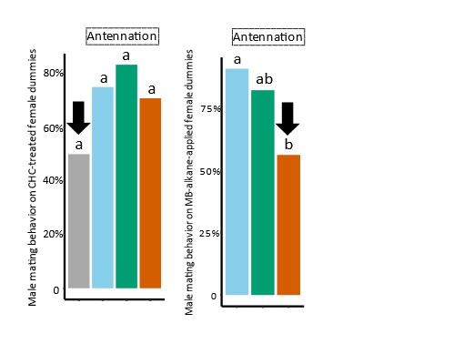
Unfortunately, the authors don't present experiments testing the effect of the non-MB alkanes fractions of the CHC extracts on male behavior toward females. As such, they are not able to (and didn't) conclude that the MB-alkane is necessary to trigger the sexual behaviors of males. I believe testing this would have significantly enhanced the significance of this work. I would also have found it interesting for the authors to comment on whether they observe aggressive behavior of males towards females (live or dead) and/or whether such behavior is expected or not in inter-individual interactions in parasitoids wasps.
In our experiment, we focus on the function of the MB-alkane fraction in female CHC profiles, and we comprehensibly demonstrate in figure 4 that the MB-alkane fraction from WT females alone is sufficient to trigger mating behavior coherent with that on alive and untreated female dummies. Therefore, we do not completely understand the reviewer’s concern about us not being ” able to (and didn't) conclude that the MB-alkane is necessary to trigger the sexual behaviors of males”. We appreciate the suggestion from the reviewer of testing the non-MB alkanes (n-alkanes and n-alkenes). However, due to the experimental procedure of separating the CHC compound class fractions through elution with molecular sieves, it was not possible for us to retrieve either the whole n-alkane or n-alkene fraction remaining bound to the sieves after separation). The role of n-alkenes in N. vitripennis is however considered in the discussion, as a deterrent for homosexual interactions between males (Wang et al. 2022a). Moreover, we did not observe aggressive behavior of males towards live or dead females.
CHCs are used by insects to signal and/or recognize various traits of targets of interest, including species or groups of origin, fertility, etc. The authors claim that their experiments show the sexual attractiveness of females can be encoded in the specific ratio of MB alkanes. While I understand how they come to this conclusion, I am somewhat concerned. The authors very quickly discuss their results in light of the literature about the role of CHCs (and notably MB alkanes) in various recognition behaviors in Hymenoptera, including conspecific recognition. Previous work (cited by the authors) has shown that males recognize males from females using an alkene (Z9C31). As such, it remains possible that the "sexual attractiveness" of N. vitripennis females for males relies on them not being males and being from the right species as well. The authors do not address the question of whether the CHCs (and the MB alkanes in particular) of females signal their sex or their species. While I acknowledge that responding to this question is beyond the scope of this work, I also strongly believe that it should be discussed in the manuscript. Otherwise, non-specialist readers would not be able to understand what I believe is one of the points that could temper the conclusions from this work.
We acknowledge the reviewer’s insight about the MB alkanes in signaling sex or species in N. vitripennis, and now include this aspect in our revised discussion (line 324-330). Moreover, we clearly demonstrate that n-alkenes have been reduced to minute trace components after our compound class separation, and the males still do not display courtship and copulation behaviors similar to WT females, thus strongly indicating that the n-alkenes do not play a role when relying solely on the changed MB-alkane patterns, further strengthening our main argument.
References
Benjamini, Y. and D. Yekutieli. 2001. The control of the false discovery rate in multiple testing under dependency. Ann. Stat. 29:1165-1188.
Buellesbach, J., J. Gadau, L. W. Beukeboom, F. Echinger, R. Raychoudhury, J. H. Werren, and T. Schmitt. 2013. Cuticular hydrocarbon divergence in the jewel wasp Nasonia: Evolutionary shifts in chemical communication channels? J. Evol. Biol. 26:2467-2478.
Buellesbach, J., C. Greim, and T. Schmitt. 2014. Asymmetric interspecific mating behavior reflects incomplete prezygotic isolation in the jewel wasp genus Nasonia. Ethology 120:834-843.
Buellesbach, J., H. Holze, L. Schrader, J. Liebig, T. Schmitt, J. Gadau, and O. Niehuis. 2022. Genetic and genomic architecture of species-specific cuticular hydrocarbon variation in parasitoid wasps. Proc. R. Soc. B 289:20220336.
Engl, T., N. Eberl, C. Gorse, T. Krüger, T. H. P. Schmidt, R. Plarre, C. Adler, and M. Kaltenpoth. 2018. Ancient symbiosis confers desiccation resistance to stored grain pest beetles. Mol. Ecol. 27:2095-2108.
Ferveur, J. F., J. Cortot, K. Rihani, M. Cobb, and C. Everaerts. 2018. Desiccation resistance: effect of cuticular hydrocarbons and water content in Drosophila melanogaster adults. Peerj 6.
Lammers, M., K. Kraaijeveld, J. Mariën, and J. Ellers. 2019. Gene expression changes associated with the evolutionary loss of a metabolic trait: lack of lipogenesis in parasitoids. BMC Genom. 20:309.
Mair, M. M., V. Kmezic, S. Huber, B. A. Pannebakker, and J. Ruther. 2017. The chemical basis of mate recognition in two parasitoid wasp species of the genus Nasonia. Entomol. Exp. Appl. 164:1-15.
Wang, Y., W. Sun, S. Fleischmann, J. G. Millar, J. Ruther, and E. C. Verhulst. 2022a. Silencing Doublesex expression triggers three-level pheromonal feminization in Nasonia vitripennis males. Proc. R. Soc. B 289:20212002.
Wang, Z., J. P. Receveur, J. Pu, H. Cong, C. Richards, M. Liang, and H. Chung. 2022b. Desiccation resistance differences in Drosophila species can be largely explained by variations in cuticular hydrocarbons. eLife 11:e80859.
Author Response
Reviewer #1 (Public Review):
In this manuscript, the authors investigate the genes involved in the retention of eggs in Aedes aegypti females. They do so by identifying two candidate genes that are differentially expressed across the different reproductive phases and also show that the transcripts of those two genes are present in ovaries and in the proteome. Overall, I think this is interesting and impressive work that characterizes the function of those two specific protein-coding genes thoroughly. I also really enjoyed the figures. Although they were a bit packed, the visuals made it easy to follow the authors' arguments. I have a few concerns and suggested changes, listed below.
1) These two genes/loci are definitely rapidly evolving. However, that does not automatically imply that positive selection has occurred in these genes. Clearly, you have demonstrated that these gene sequences might be important for fitness in Aedes aegypti. However, if these happen to be disordered proteins, then they would evolve rapidly, i.e., under fewer sequence constraints. In such a scenario, dN/dS values are likely to be high. Another possibility is that as these are expressed only in one tissue and most likely not expressed constitutively, they could be under relaxed constraints relative to all other genes in the genome. For instance, we know that average expression levels of protein-coding genes are highly correlated with their rate of molecular evolution (Drummond et al., 2005). Moreover, there have clearly been genome rearrangements and/or insertion/deletions in the studied gene sequences between closely- related species (as you have nicely shown), thus again dN/dS values will naturally be high. Thus, high values of dN/dS are neither surprising nor do they directly imply positive selection in this case. If the authors really want to investigate this further, they can use the McDonald Kreitman test (McDonald and Kreitman 1991) to ask if non- synonymous divergence is higher than expected. However, this test would require population-level data. Alternatively, the authors can simply discuss adaptation as a possibility along with the others suggested above. A discussion of alternative hypotheses is extremely important and must be clearly laid out.
We agree with the reviewer’s point that rapid evolution is not the same as positive selection. We also agree with the reviewer’s point that McDonald-Kreitman test (MK test) is more powerful than dN/dS analysis. We took advantage of a large population dataset from Rose et al. 2020. After filtering the data, we kept 454 genomes for MK tests. We found both genes are marginally significant or insignificant (tweedledee p = 0.068; tweedledum p = 0.048), despite that these are small genes and have low Pn values. This suggests that it is likely the genes evolve under positive selection.
In line with the reviewer’s suggestion, we performed another analysis using a large amount of population data. We asked if the SNP frequencies of tweedledee and tweedledum are correlated with environmental variables. We found that when compared to a distribution of 10,000 simulated genes with randomly-sampled genetic variants, both tweedledee and tweedledum showed significant correlation to multiple ecological variables reflecting climate variability, such as mean diurnal range, temperature seasonality, and precipitation seasonality (p<0.05). These results are now incorporated into the manuscript in Figure 5 and Figure 5 – Figure supplement 1.
2) The authors show that the two genes under study are important for the retention of viable eggs. However, as these genes are close to two other conserved genes (scratch and peritrophin-like gene), it is unclear to me how it is possible to rule out the contribution of the conserved genes to the same phenotype. Is it possible that the CRISPR deletion leads to the disruption of expression of one of the other important genes nearby (i.e., in a scratch or peritrophin-like gene) as the deleted region could have included a promoter region for instance, which is causing the phenotype you observe? Since all of these genes are so close to each other, it is possible that they are co-regulated and that tweedledee and tweedledum and expressed and translated along with the scratch and peritrophin-like gene. Do we know whether their expression patterns diverge and that scratch and peritrophin-like genes do not play a role in the retention of viable eggs?
This is a fair criticism; however, we think the chance that the phenotypes are caused by interrupting nearby genes is very low. First, peritrophin-like acts in the immune response, and scratch is a brain-biased transcription factor. Neither of the genes show expression in the ovary before or after blood feeding (TPM <1 or 2 are generally considered unexpressed, while scratch and peritrophin-like expression levels are overall lower than 0.1 TPM).
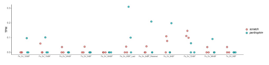
This suggests that peritrophin-like and scratch are not likely to function in the ovary. Thus, although we cannot completely rule out the gene knockout impacts regulation of very distant genes, it is unlikely. Since the mounting evidence we show in this manuscript that tweedledee and tweedledum are highly translated in the ovary after blooding feeding, under the principle of parsimony, we expect the phenotypes came from knocking out the highly expressed and translated genes.
Reviewer #2 (Public Review):
This manuscript is overall quite convincing, presenting a well- thought-out approach to candidate gene detection and systemic follow- ups on two genes that meet their candidate gene criteria. There are several major claims made by the authors, and some have more compelling evidence than others, but in general, the conclusions are quite sound. My main issues stem from how the strategy to identify genes playing a role in egg retention success has led to very particular genes being examined, and so I question some of the elements of the discussion focusing on the rapid evolution and taxon- uniqueness of the identified genes. In short, while I believe the authors have demonstrated that tweedledee and tweedledum play an important role in egg retention, I'm not sure whether this study should be taken as evidence that taxon-specific or rapidly evolving genes, in general, are responsible for this adaptation, or simply play an important role in it.
We have revised the paper to make it clearer that the focus is indeed on these two genes on not on the greater question of taxon-specific or rapidly-evolving genes.
First, the authors present evidence that Aedes aegypti females can retain eggs when a source of fresh water is lacking, confirming that females are not attracted to human forearms while retaining eggs and that up to 70% of the retained eggs hatch after retaining them for nearly a week. This ability is likely an important adaptation that allows Aedes aegypti to thrive in a broad range of conditions. The data here seem fairly compelling.
Based on this observation, the authors reason that genes responsible for the ability to retain eggs must: 1) be highly expressed in ovaries during retention, but not before or after. 2) be taxon-specific (as this behavior seems limited to Aedes aegypti). While this approach to enriching candidate genes has proven fruitful in this particular case, I'm not sure I agree with the authors' rationale. First, even genes at a low expression in the ovaries may be crucial to egg retention. Second, while egg-laying behavior is vastly varied in insects, I'm not sure focusing on taxon-restricted genes is necessary. It is entirely possible that many of the genes identified in Figure 2E play a crucial role in egg retention evolution. These are minor issues, but they are relevant to some later points made by the authors.
We regret framing the discovery of tweedledee and tweedledum in the original submission using this somewhat artificial set of filtering criteria. The reality is that the genes caught our attention for their novel sequence, tight genetic linkage, and interesting expression profile. That really is the focus of the paper, not these other peripheral questions that have been the focus of attention of the reviews. We really do apologize for all of the confusion about what this paper is about.
Nonetheless, the authors provide very compelling evidence that the two genes meeting their criteria - tweedledee and tweedledum, play an important role in egg retention. The genes seem to be expressed primarily in ovaries during egg retention (some observed expression in brain/testes is expected for any gene), and the proteins they code seem to be found in elevated quantities in both ovaries and hemolymph during and immediately after egg retention. RNA for the genes is detected in follicles within the ovary, and CRISPR knockouts of both the genes lead to a large decrease in egg viability post retention.
My earlier qualms about their search strategy relay into some issues with Figure 4, which describes how the two genes are 1) taxon- restricted and 2) have evolved very rapidly. Neither of the two statements is unexpected given the authors' search strategy. Of course, the genes examined precisely for their lack of homologs do not have any homologs. Similarly, by limiting themselves to genes that show a lack of homology (i.e. low sequence similarity) to other genes as well as genes with high expression levels in the ovaries, a higher rate of evolution is almost inevitable to infer (as ovary expressed genes tend to evolve more rapidly in mosquitoes). I agree with the authors that inferences of the evolutionary history of these genes are quite difficult because of their uniqueness, and I especially appreciate their attempts to identify homologs (although I really dislike the term "conceptualog").
We have removed our term “conceptualog” and replaced with the mor conventional “putative ortholog”
This leads to my main (fairly minor) issue of the paper - the discussion on the evolutionary history of these genes and its implications (sections "Taxon-restricted genes underlie tailored adaptations in a diverse world" and "Evolutionary histories and catering to different natural histories"). As noted, inferring this history is very difficult because the authors have focused on two rapidly evolving, taxon-restricted genes. The analyses they have performed here definitely demonstrate that the genes play an important role in egg retention, however, they do not show that taxon-restricted genes play a disproportionate role in egg retention evolution. Indeed, the only data relevant to this point would be the proportion of genes in Figure 2E that are taxon-restricted (3/9), but I'm not sure what the null expectation for this proportion for highly expressed ovary genes is to begin with. Furthermore, the extremely rapid evolution of this gene makes it hard to judge how truly taxon-restricted it is. My own search of tweedle homologs identified multiple as previously having been predicted to be "Knr4/Smi1-like", and while no similar genes are located in a similar location in melanogaster, there is generally little synteny conservation in Drosophila (for instance Bhutkar et al 2008), so I'm unsure what can really be said about their evolutionary origins/lack of homologs in Drosophila.
In short - the manuscript makes clear that tweedledee and tweedledum play an important role in egg retention in A. aegypti, nonetheless, it is not clear that this is a demonstration of how important taxon- restricted genes are to understanding the evolution of life-history strategies.
Again, we should have never framed the paper the way we did in the original version. We make no claims whatsoever that taxon-restricted genes in general should play a role in this biology, only that the two candidate genes under study influence egg viability after extended retention. We hope that the framing is clearer in this revision.
Author Response:
Reviewer #1 (Public Review):
This study sought to systematically identify the components and driving forces of transcriptome evolution in fungi that exhibit complex multicellularity (CM). The authors examined a series of parameters or expression signatures (i.e. natural antisense transcripts, allele-specific expression, RNA-editing) concluding that the best predictor of a gene behavior in the CM transcriptome was evolutionary age.
Thus, the transcriptomes of fruiting bodies showed a distinct gene-age-related stratification, where it was possible to sort out genes related to general sexual processes from those likely linked to morphogenetic aspects of the CM fruiting bodies. Notably, their results did not support a developmental hourglass, which is the rather predominant hypothesis in metazoans, including some analysis in fungi.
The studies involved analyses of new transcriptomic datasets for different developmental stages (and tissue types in some cases) of Pleurotus ostreatus and Pterula gracilis, as well as the analyses of existing datasets for other fungi.
There are diverse interesting observations such as ones regarding Allele Specific Expression (ASE), suggesting that in P. ostreatus ASE mainly occurs due to cis-regulatory allele divergence, possibly in fast evolving genes that are not under strong selection constraints, such as ones grouped in youngest gene ages categories. In addition, a large number of conserved unannotated genes among CM-specific orthogroups highlights the rather cryptic nature of CM in fungi and raises as an important area for future research.
Some of the key aspects of the analyses would need to be better exemplified such as:
– Providing a better description of the developmentally expressed TFs only in CM species
– Providing clear examples of the promoter divergence that could be the underlying mechanism behind ASE. In particular, for some cases, there may be enough information in the literature/databases to predict the appearance or disappearance of relevant cis-elements in the promoters showing the highest divergence in genes depicting the highest levels of ASE.
We appreciate the constructive comments of the Reviewer and have revised the ms in accordance with the suggestions. In particular, we link different parts of the ms better to each other, provided a more detailed discussion of developmentally expressed TFs (lines 615-621). We also provide case studies of ASE genes with cis-regulatory divergence (Figure 5 and see below), although we note that these analyses are based on inferred and not directly determined motifs, so they should be considered as preliminary.
We had considered using TF binding motifs previously, and now we gave a try to analyzing potential transcription factor binding sites in divergent promoters. We find that there are no P. ostreatus transcription factors for which motifs based on direct evidence are available; rather, all P. ostreatus motifs are based on extrapolations from experimentally determined motifs (typically in Neurospora crassa). Therefore, to avoid too general motifs, we used only those where at least 5 nucleotides show at least 80% expected frequency in the PWM-s. This left us with 158 motifs (126 excluded). High motif binding score (>=4) and self-rate (>=0.9) were also required to ignore false positive hits. Different binding ability and lack of binding in one of the parental genomes were counted for each promoter. We found that genes with allele specific expression (ASE S2 and S4) show significantly higher differences in motif binding (lacking motifs, or different binding ability) than non-ASE genes (Fig. A1). These observations show that, not only promoter divergence, but differential predicted TF binding ability is also more common among ASE genes than among non-ASE genes. This supports our conjecture that ASE arises from cis-regulatory divergence.
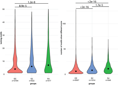
Fig A1: The left plot below shows the number of cases when the promoter of one allele of an allele pair in the two parent genomes has, but the other lacks a motif. The right plot shows the same in terms of difference in binding score.
We could find examples, such as the allele specific expression of PleosPC15_2_1031042, a Hemerythrin-like (IPR012312) protein which might be regulated by the conserved c2h2 transcription factor, containing zinc finger domain of the C2H2 type (Fig. A2). C2h2 has already been proved to be important during the initiation of primordia formation with targeted gene inactivation (Ohm et al 2011, https://pubmed.ncbi.nlm.nih.gov/21815946/). A binding site of c2h2 was detected in the upstream region of PleosPC15_2_1031042. There is a mismatch in the inferred binding motif which causes a reduced binding score in PC15 (Fig. A2/c). Indeed the PC9 nuclei contribute better to the total expression of this gene.
Despite this, and other (not shown) examples that we have found, we were not convinced about the reliability of this approach. There are many assumptions in this analysis, the positional weight matrices (PWM) that we used, are all based on indirect evidence, high number of loci these PWMs identify, uncertainty in the position of binding site from transcriptional start site, relation of difference in binding motif and expressional changes. We consider these factors to potentially contribute too much noise to the analyses for these to be robust, therefore, we are hesitant to include these results in the ms.
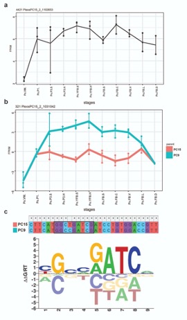
Fig A2: An example for promoter divergence a) expression of c2h2 transcription factor (TF) in P. ostreatus. b) allele-specific expression pattern of PleosPC15_2_1031042 from the two parental genomes. c) inferred binding motif of c2h2 TF and a detected potential binding site in the upstream region of PleosPC15_2_1031042 gene.
Reviewer #2 (Public Review):
The evolution of complex multicellularity represents a major developmental reprogramming, and comparing related species which differ in multicellular structures may shed light on the mechanisms involved. Here, the authors compare species of Basidiomycete fungi and focus on analyzing developmental transcriptomes to identify patterns across species. Deep RNA-Seq data is generated for two species, P. ostreatus and Pt. gracilis, sampling different developmental stages. The authors report conflicting evidence for a "developmental hourglass" using a weighted transcription index vs gene age categories. There is substantial allele-specific expression in P. ostreatus, and these genes tend to have a more recent origin, have more divergent upstream regions and coding sequences, and are enriched for developmentally regulated transcripts. Antisense transcripts have low overlap with coding regions and low conservation, and a subset show a positive or negative correlation with the overlapping gene. Comparison to a species without complex multicellular development is used to further classify the developmental program.
Overall the new transcriptional data and extensive analysis provide a thorough view of the types of transcripts that appear differentially regulated, their age, and associated gene function enrichment. The gene sets identified from this analysis as well as the potential to re-analyze this data will be useful to the community studying multicellularity in fungi. The primary insights drawn in this study relate to the dating of the developmental transcriptome, however some patterns observed with young genes and noncoding transcripts are primarily reflective of expected patterns of evolutionary time.
We appreciate the Reviewer’s nice words on our ms, we think the revised version has substantial improvements in many aspects listed above.
Reviewer #3 (Public Review):
Fungi are unique in forming complex 3D multicellular reproductive structures from 2D mycelium filaments, a property used in this paper to study the genetic changes associated with the evolution of complex 3D multicellularity. The manuscript by Merenyi et al. investigates the evolution of gene expression and genome regulation during the formation of reproductive structures (fruiting bodies) in the Agaricomycetes lineage of Fungi. Transcriptome and multicellularity evolution are very exciting fundamental questions in biology that only become accessible with recent technological developments and the appropriate analysis framework. Important perspectives include understanding how genes acquire new functions and what role plays transcriptional regulation in adaptation. The study gathers a very useful dataset to this end, and relies on generally relevant hypotheses-driven analyses.
Analysis of fruiting body transcriptome in nine species revealed that prediction from the development hourglass model (that young genes are expressed in early and late but not intermediate phases of development) verified only in a few species, including Pleurotus ostreatus. An allele-specific expression (ASE) analysis in P. ostreatus showed that young genes frequently show ASE during fruiting body development. A comparative analysis with C. neoformans, which reproduces sexually without forming fruiting body, indicates that young and old (but not intermediate) genes are likely involved specifically in fruiting body morphogenesis. A number of underlying hypothesis could be presented better, and importantly the connection between the various analyses did not appear obvious to me. Some hypotheses and reasoning therefore need clarification. Some important results from the analyses are not provided and not commented, although they are required to fully meet the manuscript's objectives.
We appreciate the Reviewer’s suggestions and have revised the ms as explained below.
- I do not clearly see the connection between the developmental hourglass model studied in the first part of the ms, and the allele-specific expression patterns in the second half of the ms. Which "phase" of the hourglass is expected to contain true CM-related genes (by contrast to general sexual processes)? Was P. ostreatus chosen for the ASE analysis because evidence for a developmental hourglass pattern was detected in this species? The conclusion that "evolutionary age predicts, to a large extent, the behaviour of a gene in the CM transcriptome" was established thanks to ASE in P. ostreatus, which was also found to be rather an exception for conforming to the hourglass model of developmental evolution. To what extent is this conclusion transferable to other Agaricomycete/fungal species?
We chose P. ostreatus because this is the only species for which the genomes of both parental strains (PC9 and PC15) are available. Although the hourglass concept is indeed a central hypothesis in animal developmental biology (though see recent critiques some (Piasecka et al 2013), our results suggest that it simply does not generally apply to fungal development. This may be due to the unique developmental mechanisms of fungi, or the independent origin(s) of CM in fungi. Our ms might have been misleading in this respect, in the revision we clarify that the ASE and hourglass analyses are independent of each other. Our interpretation of the hourglass results is that this model is not or hardly applicable for fungal development and the fact that P. ostreatus was the only species that in fact showed an hourglass did not drive our selection of this species. We inserted a note on this in the ms.
- The authors acknowledge that fruiting body-expressed genes may relate either to CM or to more general sexual functions, and that disentangling these functions is a major challenge in their study. An overview of which gene was assigned to which function is not explicit in the ms (proposed to be described in a separate publication). Do these functional gene classes show distinct transcriptome evolution patterns (hourglass model, ASE...)?
We made accessible the complete list of CM-related genes and genes with more general sexual functions in Table S2/b-c. Due to length restrictions, we do not discuss many or each of these genes here, but provided gene ontology-based overviews (Fig 8/c-d, from lines 631). To answer the question whether CM vs shared genes show distinct transcriptomic patterns, we analyzed ASE, NATs and the hourglass model separately for CM-specific and shared genes. as follows:
-hourglass: We calculated and visualised the TAI for CM-specific and Shared gene sets of P. ostreatus separately. The average value of TAI decreased a lot in Shared genes possibly due to the overrepresentation of ancient genes here, but the patterns remained similar to the original, which imply that not simply one or the other gene set drives these patterns (Fig A3).
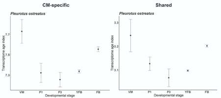
Fig A3: Transcriptome Age Index for CM-specific and Shared gene sets of P. ostreatus separately
-ASE: As we detailed in the ms, allele specific expression occurs mainly in young genes. Indeed, only 13.1% of ASE genes belong to the conserved gene sets (CMspecific: 200 and Shared: 144). Although there are more ASE genes (>2FC) among CM-specific genes, they are still underrepresented compared to young genes that are neither shared, nor CM-specific. This indicates that ASE is generally a feature of non-conserved genes and is not particularly characteristic for either conserved or CM-specific genes.
-NAT: We found that 17.3% of CM-specific (141 genes) and 18.3% of Shared genes (165 genes) overlap with antisense transcripts. Since these numbers don't differ substantially from 17.6%, which is the proportion of NATs corresponding to all protein coding genes, it implies an independent occurrence between NATs and these gene conservation groups.
3.) As far as I understand, major functions of the fruiting body transcriptome are either CM or general sexual functions. Could these genes, notably those showing ASE, play a role in general processes other than sexual development (hyphal growth, environment sensing, cell homeostasis, pathogenicity)?
Certainly, ASE might also occur in genes related to these processes. However, the processes mentioned by the Reviewer are likely associated with very conserved genes (except pathogenicity, which we can’t examine here) and our results suggest that ASE is more typical of young genes that are under weak selection. We detected ASE in 931/343 (S2/S4 genes) genes expressed in the vegetative mycelium stage of P. ostreatus. We also note that by the definition of developmentally regulated genes, we do not expect very basic fungal processes, like hyphal growth to be among the functions of the genes we identified. Genes related to such basic (housekeeping) processes usually (exceptions exist) show flat expression profiles (because they are equally important in mycelia and all fruiting body stages) and will not be picked up by our pipelines for identifying shared developmentally regulated genes.
- As stated by the authors, "the goal of this study was to systematically tease apart the components and driving forces of transcriptome evolution in CM fungi". What drives the interesting ASE pattern discovered however remains an open question at the end of the ms. The authors appropriately discuss that these patterns could be either adaptive or neutral but there is no direct evidence for any scenario in P. ostreatus. Is the expression of (some of) the young genes showing ASE required for CM? one or two case studies would allow providing support for such scenarios.
We respectfully disagree. We provide evidence that the driving force of ASE is promoter divergence (and consequently differential transcription factor binding) in genes in which it is tolerated (see conclusions, lines 708-712). Our results suggest that ASE is mostly a neutrally arising phenomenon. To get to the mechanistic bases of how promoter divergence can cause ASE (following the suggestion of Reviewer 1), we analysed putative, inferred transcription factor binding motifs in P. ostreatus and found that ASE genes had more divergence in putative TF binding sites. However, it is important to emphasise that all TF motifs we analyzed are inferred motifs and therefore these results are indicative at best.
Reviewer #4 (Public Review):
This work develops a comparative framework to test genes which support complex morphological structures and complex multicelluarity. This expands beyond simple gene sharing and phylogenomics by incorporating comparison of gene expression profiling of development of multicellular structures during sexual reproduction. This approach tests the hypothesis that genes underlying sexual reproductive structure formation are homologous and the molecular evolutionary processes that control transcriptome evolution which underlie complex multicellularity.
The approaches used are appropriate and employ modern comparative and transcriptome analyses to example allele specific expression, and evaluate an age of the evolutionary ages of genes. This work produced additional new RNAseq to examine developmental processes and combined it with existing published data to contrast fungi with either complex morphologies or yeast forms.
The strengths of work are well selected comparison organisms and efforts to have developmental stages which are appropriate comparisons.
We appreciate the Reviewer’s positive comments.
Weakness could be pointed to in how the NAT descriptions are interesting it isn't clear how they link directly to morphology variation or development. I am unclear if these are arising from new de novo promotors, are ferried by transposable elements, or if any other understanding of their genesis indicates they are more than very recent gains in a species for the most part and not part of any conserved developmental process (outside a few exemplars).
Originally, we assayed natural antisense transcripts (NAT) based on the assumption that they regulate developmental processes (e.g. Kim et al 2018 https://doi.org/10.1128/mBio.01292-18). Our analyses showed that although NATs are abundant in CM transcriptomes of fungi, they show no homology across species and so are unlikely to drive conserved developmental processes, which we are after in this ms. Rather, our data are compatible with most (but likely not all) NATs being transcriptional noise, arising from novel or random promoters. We therefore shortened this section and moved much of it to the Appendix 1.
The impact of this work will reside in how gene age intersects with variability and relative importance in CM. it will be interesting to see future work examine the functions of these genes and test how allele specific expression and specific alleles are contributing to the formation of these tissues and growth forms. I am still not sure if molecular mechanisms of how high variability in gene expression is still producing relatively uniform morphologies, or if it isn't quantification of morphological variation would be nice to link to whether ASE underlie that.
We agree that allele specific expression could influence morphologies significantly, but investigating that is beyond the scope of the current work (it would require a population genomics project). More direct evidence on allelic differences can be seen in monokaryon phenotypes, which only express one of the parental alleles. Phenotypic differences are obvious in the mycelium of the two parental monokaryons : the mycelium of PC9 is more fluffy and grows faster than that of PC15. This was reported recently by Lee et al 2021 (https://doi.org/10.1093/g3journal/jkaa008). We agree with the Reviewer that this is a very exciting future research direction.
To my read of the work, the authors achieved their goals and confirmed hypothesis about the age of genes and the variability of gene expression. I still feel there is some clarity lost in whether the findings across the large number of species compared here help inform predictions or classifications of types of genes which either have ASE or are implicated in CM. This is really work for the future as the authors have provided a detailed analysis and approach that can fuel further direction in this research area.
To address this issue we reworked the ms to make connections between ASE and CM clearer. Because ASE appears based on our results to (mostly) arise neutrally, predictions for other species are expected to be hard. On the other hand, we think we can make confident predictions on what types of genes are implicated in CM in other species, at least for conserved aspects of fruiting body development.
Author Response
Reviewer #1 (Public Review):
In this study, the authors set out to clarify the relationship between brain oscillations and different levels of speech (syllables, words, phrases) using MEG. They presented word lists and sentences and used task instructions to attempt to focus listeners' attention on different levels of linguistic analysis (syllables, words, phrases).
1) I came away with mixed feelings about the task design: following each stimulus (sentence or word list), participants were asked to (a) press a button (i.e. nothing related to what they heard, (b) indicate which of two syllables was heard, (c) indicate which of two words was heard, (d) indicate which pair of words was present in the correct order. This task is the critical manipulation in the study, as it is intended to encourage (or in the authors' words, "require") participants to focus on different timescales of speech (syllable, word, and phrase, respectively). I very much like the idea of keeping the physical stimuli unchanged, and manipulating attention through task demands - an elegant and effective approach. At the same time, I have reservations about the degree to which these task instructions altered attention during listening. My intuition is that, if I were a participant, I would just listen attentively, and then answer the question about the specific level. For example, I don't know that knowing I would be doing a "word pair" task, I would be attending at a slower rate than a "word" task, as in both cases I would be motivated to understand all of the words in the sentence. I fully acknowledge my introspection (n=1) may be flawed here, but nevertheless, any additional support validating the effect of these instructions would help the interpretation of the MEG results.
The reviewer points out that to do any task on sentences (such as a word task and a syllable task) participants’ strategy could be to understand the full meaning of the sentence and infer the lower level properties based on the understanding of the full sentence. We fully share this introspection, which would suggest that extracting sentence meaning is partly automatic (or at least a default mode of processing) and independent of the behavioral relevance. While the reviewer sees this as a downside of the design, this is part of what our study tried to disentangle (automatic versus task-dependent processing at lower frequency time-scales). If, as the reviewer points out, all processing of sentences would be automatic we should not find any effect of task (as the task should not affect the tracking response at all). We found that overall the tracking response is robust to task-induced manipulation of attention – the main effect that MI to phrases is higher for sentences than for word lists is robust across passive and task conditions. But that is not the whole story on the source level, where we do find some task effects, which indicates that task instructions do matter. This means that participants changed their strategy depending on the instructions, but that overall, tracking of linguistic structures such as phrases is automatic. We show that for the IFG MI phrasal time scales are tracked stronger during the phrase task versus the other tasks. This is also reflected in stronger STG-IFG connectivity during the phrasal versus passive task. These results speak against the interpretation of the reviewer that “task instructions“ do not “ altered attention during listening”. While there are these subtle task differences, especially in IFG, overall our findings do speak for an automatic tracking of phrasal rate structure in sentences independent of task. We therefore concluded that “automatic understanding of linguistic information, and all the processing that this entails, cannot be countered to substantially change the consequences for neural readout, even when explicitly instructing participants to pay attention to particular time-scales” (line 548-549).
The analysis steps generally seem sensible and well-suited to answering the main claims of the study. Controlling for power differences between conditions through matching was a nice feature.
2) I had a concern about accuracy differences (as seen in Figure 1) across stimulus materials and tasks. In particular, for the phrase task, participants were more accurate for sentence stimuli than word list stimuli. I think this makes a lot of sense, as a coherent sentence will be easier to remember in order than a list of words. But, I did not see accuracy taken into account in any of the analyses. These behavioral differences raise the possibility that the MEG results related to the sentence > word list contrast in phrases (which seems one of the most interesting findings in IFG) simply reflect differences in accuracy.
With the caveat of the concern regarding accuracy differences, the research goals were clear and the conclusions were generally supported by the analyses.
Thank you for pointing this out. We have now taken accuracy into account in our analysis. It did not change any of our main findings or conclusions, and strengthened the argument that tracking of phrases in sentences vs. word lists is stronger. The influence of task difficulty is a relevant point to investigate (also see point 1 of reviewer 2 and point 4 of reviewer 3). To do so we added accuracy (per participant per condition) as a factor in the mixed model (as well as all interactions with task and condition) for the MI, power, and connectivity analyses at the phrasal rate/delta band. Note that as for the passive task there is no accuracy, we removed the passive task from the analyses. We could also only run models with random intercepts (not random slopes), due to the reduced number of degrees of freedom when adding the factor accuracy to the models.
For the MI analysis we only found an effect in MTG. Specifically, there was a three-way interaction between task, condition and accuracy (F(2, 91.9) = 3.4591, p = 0.036). To follow up on this three-way interaction we split the data per task. The condition*accuracy interaction was only (uncorrected) significant for the word combination task (F(1,24.8) = 5.296, p = 0.03 (uncorrected)) and not for any other task (p>0.1). In the word combination task, we found that the difference between sentences and word lists was the strongest at high accuracies (see below figure the predicted values of the model). One way to interpret this finding is that stronger phrasal-rate MI tracking in MTG promotes phrasal-rate processing (as indicated by accuracy) more in sentences than in word lists.
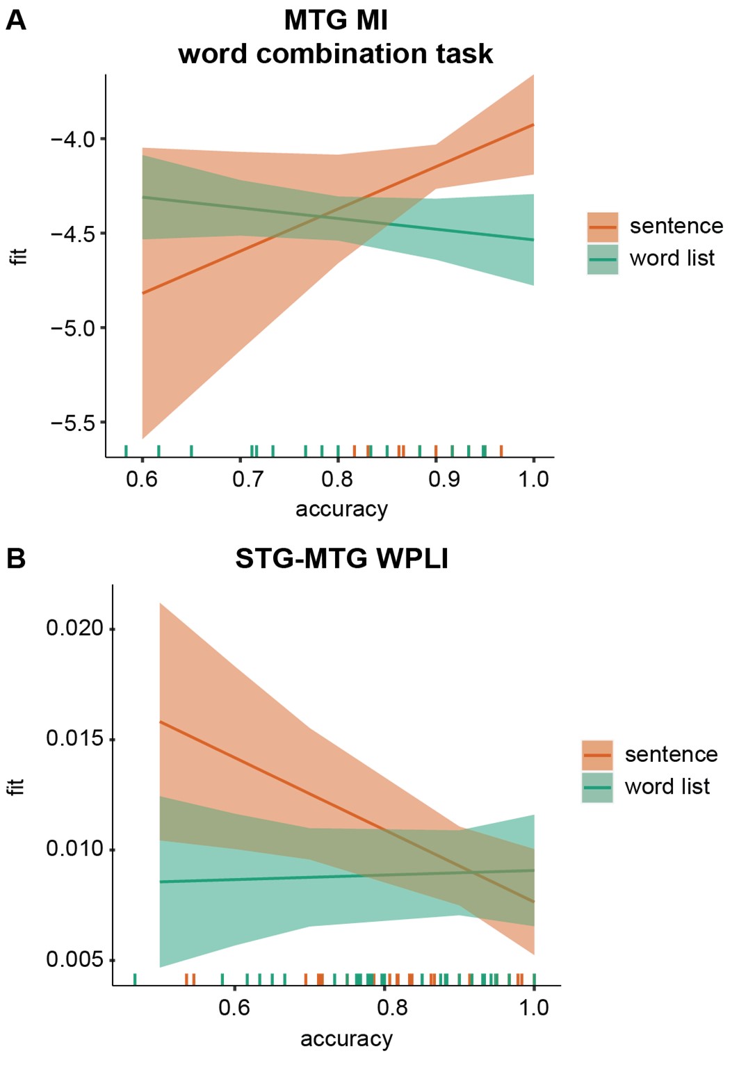
MEG – behavioral performance relation. A) Predicted values for the phrasal band MI in the MTG for the word combination task separately for the two conditions. B) Predicted values for the delta band WPLI in the STG-MTG connection separately for the two conditions. Error bars indicate the 95% confidence interval of the fit. Colored lines at the bottom indicate individual datapoints.
For power we did not find any effect of accuracy. For the connectivity analysis we found in the STG-MTG connectivity a significant conditionaccuracy interaction (F(1, 80.23)=5.19, p = 0.025). The conditionaccuracy interaction showed that lower accuracies were generally associated with stronger differences between the sentences and word lists (see figure; the opposite of the MI analysis). Thus, functional connections in the delta band are stronger during sentence processing when participants have difficulty with the task (independent of the task performed). This could indicate that low-frequency connections are more relevant for the sentence than the word list condition (as the reviewer also indicated in point 1).
After correcting for accuracy there was also a significant task condition interaction (F(2,80.01) = 3.348, p = 0.040) and a main effect of condition (F(1,80.361) = 5.809, p = 0.018). While overall there was a stronger WPLI for the sentence compared to the word list condition, the interaction seemed to indicate that this was especially the case during the word task (p = 0.005 corrected), but not for the other tasks (p>0.1).
We added the results of the accuracy analyses in the main manuscript as well as adding a dedicated section in our discussion section (page 21-22). Adding accuracy did not remove any of the effects we report in the original analyses. Therefore, none of these finding change the interpretation of the results as the task still had an influence on the MI responses of MTG and IFG. The effect of accuracy in the MTG refined the results showing that the effect was strongest there for participants with high accuracies. This relationship suggests a functional role of tracking through phase alignment for understanding phrasal structure.
The methods now read: “MEG-behavioural performance analysis: To investigate the relation between the MEG measures and the behavioural performance we repeated the analyses (MI, power, and connectivity) but added accuracy as a factor (together with the interactions with the task and condition factor). As there is no accuracy for the passive task, we removed this task from the analysis. We then followed the same analyse steps as before. Since we reduced our degree of freedom, we could however only create random intercept and not random slope models”.
The results now read: “MEG-behavioural performance relation. We found for the MI analysis a significant effect of accuracy only in the MTG. Here, we found a three-way interaction between accuracy task condition (F(2, 91.9) = 3.459, p = 0.036). Splitting up for the three different tasks we found only an uncorrected significant effect for the condition accuracy interaction for the phrasal task (F(1, 24.8) = 5.296, p = 0.03) and not for the other two tasks (p>0.1). In the phrasal task, we found that when accuracy was high, there was a stronger difference between the sentence and the word list condition compared to when accuracy was low, with stronger accuracy for the sentence condition (Figure 7A).
No relation between accuracy and power was found. For the connectivity analysis we found a significant condition accuracy interaction for the STG-MTG connection (F(1,80.23) = 5.19, p = 0.025; Figure 7B). Independent of task, when accuracy was low the difference between sentence and word lists was stronger with higher WPLI fits for the sentence condition. After correcting for accuracy there was also a significant task condition interaction (F(2,80.01) = 3.348, p = 0.040) and a main effect of condition (F(1,80.361) = 5.809, p = 0.018). While overall there was a stronger WPLI for the sentence compared to the word list condition, the interaction seemed to indicate that this was especially the case during the word task (p = 0.005), but not for the other tasks (p>0.1).”
The discussion now reads: “We found that across participants both the MI and the connectivity in temporal cortex influenced behavioural performance. Specifically, MTG-STG connections were, independent of task, related to accuracy. There was higher connectivity between MTG and STG for sentences compared to word lists at low accuracies. At high accuracies, we found that stronger MTG tracking at phrasal rates (measured with MI) for sentences compared to word lists during the word combination task. These results suggest that indeed tracking of phrasal structure in MTG is relevant to understand sentences compared to word lists. This was reflected in a general increase in delta connectivity differences when the task was difficult (Figure 7B). Participants might compensate for the difficulty using phrasal structure present in the sentence condition. When phrasal structure in sentences are accurately tracked (as measured with MI) performance is better when these rates are relevant (Figure 7A). These results point to a role for phrasal tracking for accurately understanding the higher order linguistic structure in sentences even though more research is needed to verify this. It is evident that the connectivity and tracking correlations to behaviour do not explain all variation in the behavioural performance (compare Figure 1 with 3). Plainly, temporal tracking does not explain everything in language processing. Besides tracking there are many other components important for our designated tasks, such as memory load and semantic context which are not captured by our current analyses.”
Reviewer #2 (Public Review):
In a MEG study, the authors investigate as their main question whether neural tracking at the phrasal time scale reflects linguistic structure building (testing different conditions: sentences vs. word-lists) or an attentional focus on the phrasal time scale (testing different tasks, passive listening, syllable task, word task, word combination/phrasal scale task). They perform the following analyses at brain areas (ROIs: STG, IFG, MTG) of the language network: (1) Mutual information (MI) between the acoustic envelope and the delta band neuronal signals is analyzed. (2) Power in the delta band is analyzed. (3) Connectivity is analyzed using debiased WPLI. For all analyses, linear mixed-models are separately conducted for each ROI. The main finding is that the sentence compared to the word-list condition is more strongly tracked at the phrasal scale (MI). In STG the effect was task-independent; in MTG the effect only occurred for active tasks; and in IFG additionally, the word-combining/phrasal scale task resulted in higher tracking compared to all other tasks. The authors conclude that phrasal scale neural tracking reflects linguistic processing which takes place automatically, while task-related attention contributes additionally at IFG (interpreted as combinatorial hub involved in language and non-language processing). The findings are stable when power differences are controlled. The connectivity analysis showed increased connectivity in the delta band (phrasal time scale) between IFG-STG in the phrasal-scale compared to the passive task (adding to the IFG MI findings). (Additionally, they separately analyze neural tracking at the syllabic and word time scale, which however is not in the main focus).
Major strength/weaknesses of the methods and results:
1) A major strength of the results is that part of them replicate the authors' earlier findings (i.e. higher tracking at the phrasal time scale for sentences compared to word-lists; Kaufeld et al., 2020), while they complement this earlier work by showing that the effects are due to linguistic processing and not to an attentional focus on the phrasal time scale due to the task (at least in STG and MTG; while the task plays a role for the IFG tracking). Another strength is that a power control analysis is applied, which allows excluding spurious results due to condition differences in power. A weakness of the method is that analyses were applied separately per ROI, and combined across correct/incorrect trials (if I understood correctly), no trial-based analysis was conducted (which is related to how MI is computed). Furthermore, several methodological details could be clarified in the manuscript.
The authors achieved their aims by providing evidence that neuronal tracking at the phrasal time scale in STG and MTG depends on the presence of linguistic information at this scale rather than indicating an attentional focus on this time scale due to a specific task. Their results support the conclusion. Results would be strengthened by showing that these effects are not impacted by different amounts of correct/incorrect trials across conditions (if I understood that correctly).
We thank the reviewer for her comments. It is correct that we collapsed across the correct and incorrect trials. This had various reasons (also see point 2 and 9 of reviewer 1 and point 4 of reviewer 3). First, our tasks function solely to direct participants’ attention to the various linguistic representations (syllables, words, phrases) and the timescales that they occur on. The three tasks are in a sense more control tasks to study the tracking response, and manipulate attention as tracking during spoken language comprehension occurs, rather than a case where the neural response to the tasks is itself to be studied. For example, in a typical working memory paradigm, it is only during correct trials that the relevant cognitive process occurs. In contrast, in our paradigm, it is likely that that spoken stimuli are heard and processing, in other words, sentence comprehension and word list perception occur, even during incorrect trials in the syllable condition. As such, we do not expect MI tracking responses to explain the behavioral data. However, we agree it is crucially important to show that MI differences are not a function of task performance differences.
Second, there are clear differences in difficulty level of the trials within conditions. For example, if the target question was related to the last part of the audio fragment, the task was much easier than when it was at the beginning of the audio fragment. In the syllable task, if syllables also were (by chance) a part-word, the trial was also much easier. If we were to split up in correct and incorrect we would not really infer solely processes due to accurately processing the speech fragments, but also confounded the analysis by the individual difficulty level of the trials.
To acknowledge this, we added this limitation to the methods. The methods now reads: “Note that different trials within a task were not matched for task difficulty. For example, in the syllable task syllables that make a word are much easier to recognize than syllables that do not make a word. Additionally, trials pertaining to the beginning of the sentence are more difficult than ones related to the end of the sentence due to recency effects.”.
To still investigate if overall accuracy influenced the results we did add accuracy (across participants) to the mixed models. Note that as for the passive task there is no accuracy, we removed the passive task from the analyses. We could also only run models with random intercepts (not random slopes), due to the reduced number of degrees of freedom when adding the factor accuracy to the models.
For the MI analysis we only found an effect in MTG. Specifically, there was a three-way interaction between task, condition and accuracy (F(2, 91.9) = 3.4591, p = 0.036). To follow up on this three-way interaction we split the data per task. The condition*accuracy interaction was only (uncorrected) significant for the word combination task (F(1,24.8) = 5.296, p = 0.03 (uncorrected)) and not for any other task (p>0.1). In the word combination task, we found that the difference between sentences and word lists was the strongest at high accuracies (see on the right attached figure the predicted values of the model). One way to interpret this finding is that stronger phrasal-rate MI tracking in MTG promotes phrasal-rate processing (as indicated by accuracy) more in sentences than in word lists.
For power we did not find any effect of accuracy. For the connectivity analysis we found in the STG-MTG connectivity a significant conditionaccuracy interaction (F(1, 80.23)=5.19, p = 0.025). The conditionaccuracy interaction showed that lower accuracies were generally associated with stronger differences between the sentences and word lists (see figure below; the opposite of the MI analysis). Thus, functional connections in the delta band are stronger during sentence processing when participants have difficulty with the task (independent of the task performed). This could indicate that low-frequency connections are more relevant for the sentence than the word list condition.

MEG – behavioral performance relation. A) Predicted values for the phrasal band MI in the MTG for the word combination task separately for the two conditions. B) Predicted values for the delta band WPLI in the STG-MTG connection separately for the two conditions. Error bars indicate the 95% confidence interval of the fit. Colored lines at the bottom indicate individual datapoints.
After correcting for accuracy there was also a significant task*condition interaction (F(2,80.01) = 3.348, p = 0.040) and a main effect of condition (F(1,80.361) = 5.809, p = 0.018). While overall there was a stronger WPLI for the sentence compared to the word list condition, the interaction seemed to indicate that this was especially the case during the word task (p = 0.005 corrected), but not for the other tasks (p>0.1).
We added the results of the accuracy analyses in the main manuscript as well as adding a dedicated section in our discussion section (page 21-22). Adding accuracy did not remove any of the effects we report in the original analyses. Therefore, none of these finding change the interpretation of the results as the task still had an influence on the MI responses of MTG and IFG. The effect of accuracy in the MTG refined the results showing that the effect was strongest there for participants with high accuracies. This relationship suggests a functional role of tracking through phase alignment for understanding phrasal structure.
The methods now read: “MEG-behavioural performance analysis: To investigate the relation between the MEG measures and the behavioural performance we repeated the analyses (MI, power, and connectivity) but added accuracy as a factor (together with the interactions with the task and condition factor). As there is no accuracy for the passive task, we removed this task from the analysis. We then followed the same analyse steps as before. Since we reduced our degree of freedom, we could however only create random intercept and not random slope models”.
The results now read: “MEG-behavioural performance relation. We found for the MI analysis a significant effect of accuracy only in the MTG. Here, we found a three-way interaction between accuracytaskcondition (F(2, 91.9) = 3.459, p = 0.036). Splitting up for the three different tasks we found only an uncorrected significant effect for the condition*accuracy interaction for the phrasal task (F(1, 24.8) = 5.296, p = 0.03) and not for the other two tasks (p>0.1). In the phrasal task, we found that when accuracy was high, there was a stronger difference between the sentence and the word list condition compared to when accuracy was low, with stronger accuracy for the sentence condition (Figure 7A).
No relation between accuracy and power was found. For the connectivity analysis we found a significant conditionaccuracy interaction for the STG-MTG connection (F(1,80.23) = 5.19, p = 0.025; Figure 7B). Independent of task, when accuracy was low the difference between sentence and word lists was stronger with higher WPLI fits for the sentence condition. After correcting for accuracy there was also a significant taskcondition interaction (F(2,80.01) = 3.348, p = 0.040) and a main effect of condition (F(1,80.361) = 5.809, p = 0.018). While overall there was a stronger WPLI for the sentence compared to the word list condition, the interaction seemed to indicate that this was especially the case during the word task (p = 0.005), but not for the other tasks (p>0.1).”
The discussion now reads: “We found that across participants both the MI and the connectivity in temporal cortex influenced behavioural performance. Specifically, MTG-STG connections were, independent of task, related to accuracy. There was higher connectivity between MTG and STG for sentences compared to word lists at low accuracies. At high accuracies, we found that stronger MTG tracking at phrasal rates (measured with MI) for sentences compared to word lists during the word combination task. These results suggest that indeed tracking of phrasal structure in MTG is relevant to understand sentences compared to word lists. This was reflected in a general increase in delta connectivity differences when the task was difficult (Figure 7B). Participants might compensate for the difficulty using phrasal structure present in the sentence condition. When phrasal structure in sentences are accurately tracked (as measured with MI) performance is better when these rates are relevant (Figure 7A). These results point to a role for phrasal tracking for accurately understanding the higher order linguistic structure in sentences even though more research is needed to verify this. It is evident that the connectivity and tracking correlations to behaviour do not explain all variation in the behavioural performance (compare Figure 1 with 3). Plainly, temporal tracking does not explain everything in language processing. Besides tracking there are many other components important for our designated tasks, such as memory load and semantic context which are not captured by our current analyses.”
The findings are an important contribution to the ongoing debate in the field whether neuronal tracking at the phrasal time scale indicates linguistic structure processing or more general processes (e.g. chunking).
Reviewer #3 (Public Review):
This manuscript presents a MEG study aiming to investigate whether neural tracking of phrasal timescales depends on automatic language processing or specific tasks related to temporal attention. The authors collected MEG data of 20 participants as they listened to naturally spoken sentences or word lists during four different tasks (passive listening vs. syllable task vs. word tasks vs. phrase task). Based on mutual information and Connectivity analysis, the authors found that (1) neural tracking at the phrasal band (0.8-1.1 Hz) was significantly stronger for the sentence condition compared to the word list condition across the classical language network, i.e., STG, MTG, and IFG; (2) neural tracking at the phrasal band was (at least tend significantly) stronger for phrase task than other tasks in the IFG; (3) the IFG-STG connectivity was increased in the delta-band for the phrase task. Ultimately, the authors concluded that neural tracking of phrasal timescales relied on both automatic language processing and specific tasks.
Overall, this study is trying to tackle an interesting question related to the contributing factors for neural tracking of linguistic structures. The study procedure and analyses are well executed, and the conclusions of this paper are mostly well supported by data. However, I do have several major concerns.
- The title of the manuscript uses the description "tracking of hierarchical linguistic structure". In general, hierarchical linguistic structures involve multiple linguistic units with different timescales, such as syllables, words, phrases, and sentences. In this study, however, the main analysis only focused on the phrasal band (0.8-1.1 Hz). It seemed that there was no significant stimulus- or task-effect on the word band or syllabic band (supplementary figures). Therefore, it is highly recommended that the authors modify the related descriptions, or explain why neural tracking of phrases can represent neural tracking of hierarchical linguistic structures in the current study.
We thank the reviewer for this comment. We meant to refer to the task manipulation directing attention to different levels of representation across the linguistic hierarchy. We have changed the title to “Neural tracking of phrases during spoken language comprehension is automatic and task-dependent.” We hope this resolves any inadvertent confusion we created. Furthermore, throughout the manuscript we ensure to talk about effect occurring for phrasal tracking at low frequency bands at not across any hierarchical linguistic structure. We agree that our findings cannot speak for any task-dependent effects along the hierarchy, only that at the phrasal level there is a difference between sentences and word lists.
- In Methods, the authors employed MI analyses on three frequency bands: 0.8-1.1 Hz for the phrasal band, 1.9-2.8 Hz for the word band, and 3.5-5.0 Hz for the syllabic band (line 191-192). As the timescales of linguistic units are various and overlapped in natural speech, I wonder how the authors define the boundaries of these frequency bands, and whether these bands are proper for the naturally spoken stimuli in the current study. These important details should be clarified.
The frequency bands of the MI analysis were based on the stimuli, or in other words, are data driven. They reflect the syllabic, word, and phrasal rates in our stimulus set (calculated in Kaufeld et al., 2020). They were calculated by annotating the sentences by syllables, words, and phrasal and converting the rate of the linguistic units to frequency ranges. The information has been added to the manuscript. We acknowledge that unlike our stimulus set in natural speech the boundaries of these bands can overlap and now also state this (“While in our stimulus set the boundaries of the linguistic levels did not overlap, in natural speech the brain has an even more difficult task as there is no one-to-one match between band and linguistic unit [26]”, line number 211-213).
- What is missing in the manuscript are the explanations of the correlation between behavioral performance and neural tracking. In Results, the behavioral performance shows significant differences across the active tasks (Figure 1), but the MI differences across the tasks are relatively weak in IFG (Figure 3). In addition, the behavioral performance only shows significant differences between the sentence and word list conditions during the phrasal task, but the MI differences between the conditions are significant in MTG during the syllabic, word, and phrasal tasks. Explanations for these inconsistent results are expected.
We answer this point together with point 4 below where we analyze the behavioral performance and the MEG responses.
- Since the behavioral performance of these active tasks is likely related to the temporal attention to relevant timescales of different linguistic units, I wonder whether there exist underlying neural correlates of behavioral performance (e.g., significant correlation between performance and mutual information). If so, it may be interesting and bring a new bright spot for the current study.
The influence of task difficulty is a relevant point to investigate (also see point 1 of reviewer 2 and point 4 of reviewer 3). To do so we added accuracy (per participant per condition) as a factor in the mixed model (as well as all interactions with task and condition) for the MI, power, and connectivity analyses at the phrasal rate/delta band. Note that as for the passive task there is no accuracy, we removed the passive task from the analyses. We could also only run models with random intercepts (not random slopes), due to the reduced number of degrees of freedom when adding the factor accuracy to the models.
For the MI analysis we only found an effect in MTG. Specifically, there was a three-way interaction between task, condition and accuracy (F(2, 91.9) = 3.4591, p = 0.036). To follow up on this three-way interaction we split the data per task. The condition*accuracy interaction was only (uncorrected) significant for the word combination task (F(1,24.8) = 5.296, p = 0.03 (uncorrected)) and not for any other task (p>0.1). In the word combination task, we found that the difference between sentences and word lists was the strongest at high accuracies (see the below figure the predicted values of the model). One way to interpret this finding is that stronger phrasal-rate MI tracking in MTG promotes phrasal-rate processing (as indicated by accuracy) more in sentences than in word lists.

MEG – behavioral performance relation. A) Predicted values for the phrasal band MI in the MTG for the word combination task separately for the two conditions. B) Predicted values for the delta band WPLI in the STG-MTG connection separately for the two conditions. Error bars indicate the 95% confidence interval of the fit. Colored lines at the bottom indicate individual datapoints.
For power we did not find any effect of accuracy. For the connectivity analysis we found in the STG-MTG connectivity a significant conditionaccuracy interaction (F(1, 80.23)=5.19, p = 0.025). The conditionaccuracy interaction showed that lower accuracies were generally associated with stronger differences between the sentences and word lists (see figure attached; the opposite of the MI analysis). Thus, functional connections in the delta band are stronger during sentence processing when participants have difficulty with the task (independent of the task performed). This could indicate that low-frequency connections are more relevant for the sentence than the word list condition.
After correcting for accuracy there was also a significant task*condition interaction (F(2,80.01) = 3.348, p = 0.040) and a main effect of condition (F(1,80.361) = 5.809, p = 0.018). While overall there was a stronger WPLI for the sentence compared to the word list condition, the interaction seemed to indicate that this was especially the case during the word task (p = 0.005 corrected), but not for the other tasks (p>0.1).
We added the results of the accuracy analyses in the main manuscript as well as adding a dedicated section in our discussion section (page 21-22). Adding accuracy did not remove any of the effects we report in the original analyses. Therefore, none of these finding change the interpretation of the results as the task still had an influence on the MI responses of MTG and IFG. The effect of accuracy in the MTG refined the results showing that the effect was strongest there for participants with high accuracies. This relationship suggests a functional role of tracking through phase alignment for understanding phrasal structure.
While the findings can explain some behavioral effects, we agree with the reviewer that the behavioral results and the MI results don’t align. We note that our use of tasks to guide attention to different timescales and linguistic representations differs from the use of, for example, a working memory task where only the correct trials contain the relevant cognitive process. In working memory type paradigms, the MEG data should indeed explain the behavioral response. Our study was designed to test for effects of task demands on the neural tracking response to speech and language. As we are only using the tasks to control attention, we do not attempt to explain behavior through the MEG data or differences in MI.
Thus, the phrasal tracking cannot explain all of the behavioral results (point 3). It is at this point unclear what could have caused this effect, but it quite likely that neural sources outside the speech and language ROIs we selected are in play. We discuss this now.
The methods now read: “MEG-behavioural performance analysis: To investigate the relation between the MEG measures and the behavioural performance we repeated the analyses (MI, power, and connectivity) but added accuracy as a factor (together with the interactions with the task and condition factor). As there is no accuracy for the passive task, we removed this task from the analysis. We then followed the same analyse steps as before. Since we reduced our degree of freedom, we could however only create random intercept and not random slope models”.
The results now read: “MEG-behavioural performance relation. We found for the MI analysis a significant effect of accuracy only in the MTG. Here, we found a three-way interaction between accuracytaskcondition (F(2, 91.9) = 3.459, p = 0.036). Splitting up for the three different tasks we found only an uncorrected significant effect for the condition*accuracy interaction for the phrasal task (F(1, 24.8) = 5.296, p = 0.03) and not for the other two tasks (p>0.1). In the phrasal task, we found that when accuracy was high, there was a stronger difference between the sentence and the word list condition compared to when accuracy was low, with stronger accuracy for the sentence condition (Figure 7A).
No relation between accuracy and power was found. For the connectivity analysis we found a significant conditionaccuracy interaction for the STG-MTG connection (F(1,80.23) = 5.19, p = 0.025; Figure 7B). Independent of task, when accuracy was low the difference between sentence and word lists was stronger with higher WPLI fits for the sentence condition. After correcting for accuracy there was also a significant taskcondition interaction (F(2,80.01) = 3.348, p = 0.040) and a main effect of condition (F(1,80.361) = 5.809, p = 0.018). While overall there was a stronger WPLI for the sentence compared to the word list condition, the interaction seemed to indicate that this was especially the case during the word task (p = 0.005), but not for the other tasks (p>0.1).”
The discussion now reads: “We found that across participants both the MI and the connectivity in temporal cortex influenced behavioural performance. Specifically, MTG-STG connections were, independent of task, related to accuracy. There was higher connectivity between MTG and STG for sentences compared to word lists at low accuracies. At high accuracies, we found that stronger MTG tracking at phrasal rates (measured with MI) for sentences compared to word lists during the word combination task. These results suggest that indeed tracking of phrasal structure in MTG is relevant to understand sentences compared to word lists. This was reflected in a general increase in delta connectivity differences when the task was difficult (Figure 7B). Participants might compensate for the difficulty using phrasal structure present in the sentence condition. When phrasal structure in sentences are accurately tracked (as measured with MI) performance is better when these rates are relevant (Figure 7A). These results point to a role for phrasal tracking for accurately understanding the higher order linguistic structure in sentences even though more research is needed to verify this. It is evident that the connectivity and tracking correlations to behaviour do not explain all variation in the behavioural performance (compare Figure 1 with 3). Plainly, temporal tracking does not explain everything in language processing. Besides tracking there are many other components important for our designated tasks, such as memory load and semantic context which are not captured by our current analyses.”
Author Response*
Reviewer #3 (Public Review):
AAA protein are involved in a variety of cellular activity. They all share the same structural fold and still they are all incredibly specialised. This study works towards the direction of understanding the unique specialisation of the AAA protein ATAD1. While the general mechanism of substrate threading by AAA proteins is by now fairly well-elucidated, it remains to describe and understand the finer structural protein details that make each specific AAA perform unfolding (threading) of certain substrate rather than others. Additionally, regulation and stabilisation of each AAA is also finely regulated by specific subdomain.
This work is definitively strong in addressing these two points for ATAD1.
The structural data are solid and the analysis of the pore loops residues and the role of a11 overall convincing.
1) The cell fluorescence microscopy assay is a very good tool for checking in the cell the hypothesis risen by analysing of the structure. However, the assay is currently only based on the localisation of the Gos28 substrate, which leaves open the possibility that ATAD1 a11 mutants will have a different phenotype on different substrates.
We agree with the reviewer that it would be interesting to test ATAD1’s activity on other known substrates. To do that, we picked Pex26, an established tail-anchored protein substrate of ATAD1. We stably expressed EGFP-Pex26 in ATAD1-/- cells and tested the effect of ATAD1 expression on Pex26 mislocalization. As shown in the figure below, we found that although the general trend observed for Gos28 also holds true for Pex26, the measured PCC values clearly have a bimodal distribution, with some cells showing the complete mislocalization (PCC = 1.0) of Pex26. One exciting possibility to explain this result is that Pex26 is important in peroxisome biogenesis. Once enough Pex26 is mislocalized to the mitochondria, peroxisomal biogenesis becomes impaired, thus causing less Pex26 to be correctly inserted. A partial impairment in Pex26 peroxisomal insertion in turn creates a vicious cycle that leads to the complete mislocalization of Pex26. It will be an interesting to follow up on the cause of this bimodal distribution, which, however, is beyond the scope of this paper.
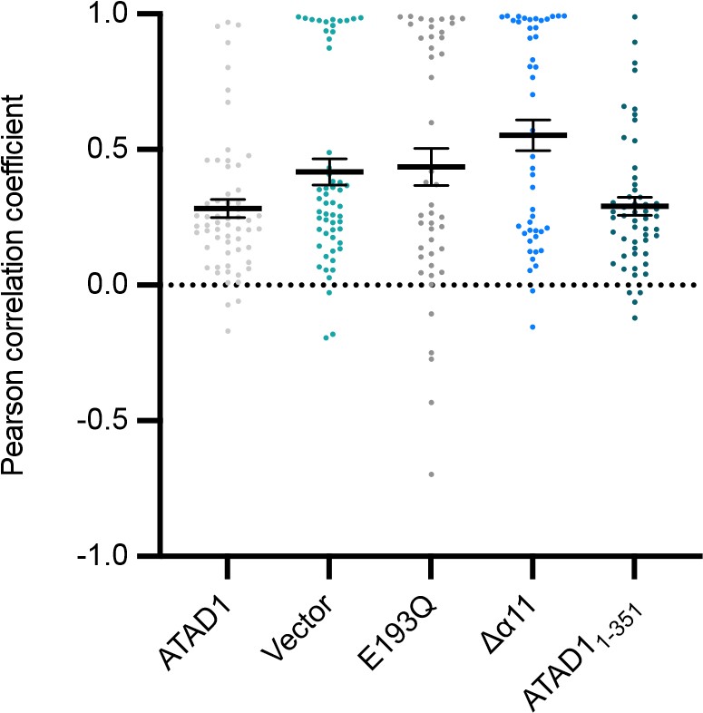
*Quantification of live-cell imaging showing using the localization of EGFP-Pex26 as a readout. Mean Pearson correlation coefficient (PCC) values and the SEM between EGFP-Pex26 and the mitochondria when expressing the ATAD1 variants indicated. Individual cell PCC values are represented as a single dot. *
Author Response:
Reviewer #1 (Public Review):
[...] While the study is addressing an interesting topic, I also felt this manuscript was limited in novel findings to take away. Certainly the study clearly shows that substitution saturation is achieved at synonymous CpG sites. However, subsequent main analyses do not really show anything new: the depletion of segregating sites in functional versus neutral categories (Fig 2) has been extensively shown in the literature and polymorphism saturation is not a necessary condition for observing this pattern.
We agree with the reviewer that many of the points raised were appreciated previously and did not mean to convey another impression. Our aim was instead to highlight some unique opportunities provided by being at or very near saturation for mCpG transitions. In that regard, we note that although depletion of variation in functional categories is to be expected at any sample size, the selection strength that this depletion reflects is very different in samples that are far from saturated, where invariant sites span the entire spectrum from neutral to lethal. Consider the depletion per functional category relative to synonymous sites in the adjoining plot in a sample of 100k: ~40% of mCpG LOF sites do not have T mutations. From our Fig. 4 and b, it can be seen that these sites are associated with a much broader range of hs values than sites invariant at 780k, so that information about selection at an individual site is quite limited (indeed, in our p-value formulation, these sites would be assigned p≤0.35, see Fig. 1). Thus, only now can we really start to tease apart weakly deleterious mutations from strongly deleterious or even embryonic lethal mutations. This allows us to identify individual sites that are most likely to underlie pathogenic mutations and functional categories that harbor deleterious variation at the extreme end of the spectrum of possible selection coefficients. More generally, saturation is useful because it allows one to learn about selection with many fewer untested assumptions than previously feasible.
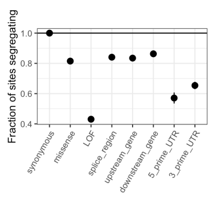
Similarly, the diminishing returns on sampling new variable sites has been shown in previous studies, for example the first "large" human datasets ca. 2012 (e.g. Fig 2 in Nelson et al. 2012, Science) have similar depictions as Figure 3B although with smaller sample sizes and different approaches (projection vs simulation in this study).
We agree completely: diminishing returns is expected on first principles from coalescent theory, which is why we cited a classic theory paper when making that point in the previous version of the manuscript. Nonetheless, the degree of saturation is an empirical question, since it depends on the unknown underlying demography of the recent past. In that regard, we note that Nelson et al. predict that at sample sizes of 400K chromosomes in Europeans, approximately 20% of all synonymous sites will be segregating at least one of three possible alleles, when the observed number is 29%. Regardless, not citing Nelson et al. 2012 was a clear oversight on our part, for which we apologize; we now cite it in that context and in mentioning the multiple merger coalescent.
There are some simulations presented in Fig 4, but this is more of a hypothetical representation of the site-specific DFE under simulation conditions roughly approximating human demography than formal inference on single sites. Again, these all describe the state of the field quite well, but I was disappointed by the lack of a novel finding derived from exploiting the mutation saturation properties at methylated CpG sites.
As noted above, in our view, the novelty of our results lies in their leveraging saturation in order to identify sites under extremely strong selection and make inferences about selection without the need to rely on strong, untested assumptions.
However, we note that Fig 4 is not simply a hypothetical representation, in that it shows the inferred DFE for single mCpG sites for a fixed mutation rate and given a plausible demographic model, given data summarized in terms of three ranges of allele frequency (i.e., = 0, between 1 and 10 copies, or above 10 copies). One could estimate a DFE across all sites from those summaries of the data (i.e., from the proportion of mCpG sites in each of the three frequency categories), by weighting the three densities in Fig 4 by those proportions. That is, in fact, what is done in a recent preprint by Dukler et al. (2021, BioRxiv): they infer the DFE from two summaries of the allele frequency spectrum (in bins of sites), the proportion of invariant sites and the proportion of alleles at 1-70 copies, in a sample of 70K chromosomes.
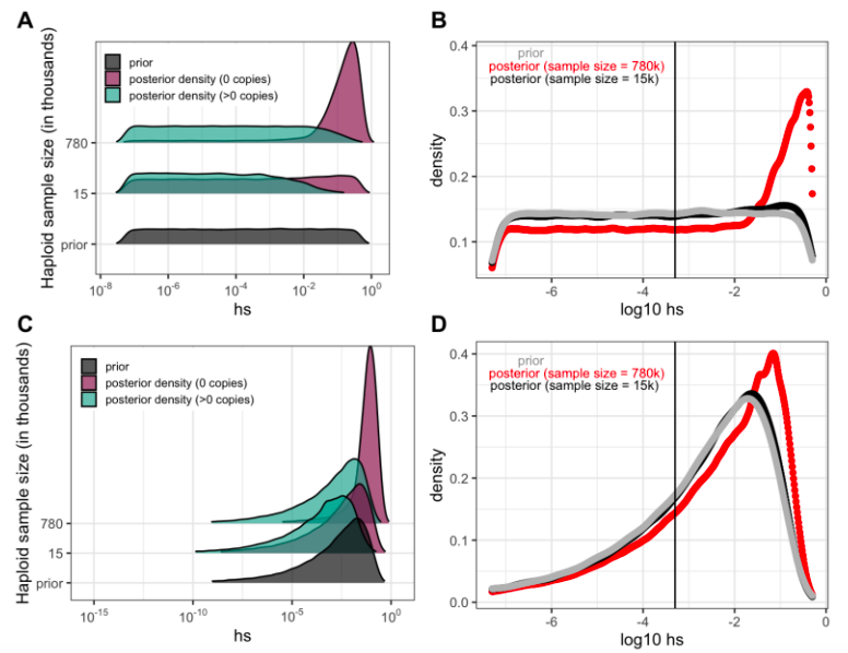
To illustrate how something similar could be done with Fig. 4 based on individual sites, we obtain an estimate of the DFE for LOF mutations (shown in Panel B and D for two different prior distributions on hs) by weighting the posterior densities in Panel A by the fraction of LOF mutations that are segregating (73% at 780K; 9% at 15K) and invariant (27% and 91% respectively); in panel C, we show the same for a different choice of prior. For the smaller sample size considered, the posterior distribution recapitulates the prior, because there is little information about selection in whether a site is observed to be segregating or invariant, and particularly about strong selection. In the sample of 780K, there is much more information about selection in a site being invariant and therefore, there is a shift towards stronger selection coefficients for LOF mutations regardless of the prior.
Our goal was to highlight these points rather than infer a DFE using these two summaries, which throw out much of the information in the data (i.e., the allele frequency differences among segregating sites). In that regard, we note that the DFE inference would be improved by using the allele frequency at each of 1.1 million individual mCpG sites in the exome. We outline this next step in the Discussion but believe it is beyond the scope of our paper, as it is a project in itself – in particular it would require careful attention to robustness with regard to both the demographic model (and its impact on multiple hits), biased gene conversion and variability in mutation rates among mCpG sites. We now make these points explicitly in the Outlook.
Similarly, I felt the authors posed a very important point about limitations of DFE inference methods in the Introduction but ended up not really providing any new insights into this problem. The authors argue (rightly so) that currently available DFE estimates are limited by both the sparsity of polymorphisms and limited flexibility in parametric forms of the DFE. However, the nonsynonymous human DFE estimates in the literature appear to be surprisingly robust to sample size: older estimates (Eyre-Walker et al. 2006 Genetics, Boyko et al. 2008 PLOS Genetics) seem to at least be somewhat consistent with newer estimates (assuming the same mutation rate) from samples that are orders of magnitude larger (Kim et al. 2017 Genetics).
We are not quite sure what the reviewer has in mind by “somewhat consistent,” as Boyko et al. estimate that 35% of non-synonymous mutations have s>10^-2 while Kim et al. find that proportion to be “0.38–0.84 fold lower” than the Boyko et al. estimate (see, e.g., Fig. 4 in Kim et al., 2017). Moreover, the preprint by Dukler et al. mentioned above, which infers the DFE based on ~70K chromosomes, finds estimates inconsistent with those of Kim et al. (see SOM Table 2 and SOM Figure S5 in Dukler et al., 2021).
More generally, given that even 70K chromosomes carry little information about much of the distribution of selection coefficients (see our Fig. 4), we expect that studies based on relatively sample sizes will basically recover something close to their prior; therefore, they should agree when they use the same or similar parametric forms for the distribution of selection coefficients and disagree otherwise. The dependence on that choice is nicely illustrated in Kim et al., who consider different choices and then perform inference on the same data set and with the same fixed mutation rate for exomes; depending on their choice anywhere between 5%-28% of non-synonymous changes are inferred to be under strong selection with s>=10^-2 (see their Table S4).
Whether a DFE inferred under polymorphism saturation conditions with different methods is different, and how it is different, is an issue of broad and immediate relevance to all those conducting population genomic simulations involving purifying selection. The analyses presented as Fig 4A and 4B kind of show this, but they are more a demonstration of what information one might have at 1M+ sample sizes rather than an analysis of whether genome-wide nonsynonymous DFE estimates are accurate. In other words, this manuscript makes it clear that a problem exists, that it is a fundamental and important problem in population genetics, and that with modern datasets we are now poised to start addressing this problem with some types of sites, but all of this is already very well-appreciated except for perhaps the last point.
At least a crude analysis to directly compare the nonsynonymous genome-wide DFE from smaller samples to the 780K sample would be helpful, but it should be noted that these kinds of analyses could be well beyond the scope of the current manuscript. For example, if methylated nonsynonymous CpG sites are under a different level of constraint than other nonsynonymous sites (Fig. S14) then comparing results to a genome-wide nonsynonymous DFE might not make sense and any new analysis would have to try and infer a DFE independently from synonymous/nonsynonymous methylated CpG sites.
We are not sure what would be learned from this comparison, given that Figure 4 shows that, at least with an uninformative prior, there is little information about the true DFE in samples, even of tens of thousands of individuals. Thus, if some of the genome-wide nonsynonymous DFE estimates based on small sample sizes turn out to be accurate, it will be because the guess about the parametric shape of the DFE was an inspired one. In our view, that is certainly possible but not likely, given that the shape of the DFE is precisely what the field has been aiming to learn and, we would argue, what we are now finally in a position to do for CpG mutations in humans.
Reviewer #2 (Public Review):
This manuscript presents a simple and elegant argument that neutrally evolving CpG sites are now mutationally saturated, with each having a 99% probability of containing variation in modern datasets containing hundreds of thousands of exomes. The authors make a compelling argument that for CpG sites where mutations would create genic stop codons or impair DNA binding, about 20% of such mutations are strongly deleterious (likely impairing fitness by 5% or more). Although it is not especially novel to make such statements about the selective constraint acting on large classes of sites, the more novel aspect of this work is the strong site-by-site prediction it makes that most individual sites without variation in UK Biobank are likely to be under strong selection.
The authors rightly point out that since 99% of neutrally evolving CpG sites contain variation in the data they are looking at, a CpG site without variation is likely evolving under constraint with a p value significance of 0.01. However, a weakness of their argument is that they do not discuss the associated multiple testing problem-in other words, how likely is it that a given non synonymous CpG site is devoid of variation but actually not under strong selection? Since one of the most novel and useful deliverables of this paper is single-base-pair-resolution predictions about which sites are under selection, such a multiple testing correction would provide important "error bars" for evaluating how likely it is that an individual CpG site is actually constrained, not just the proportion of constrained sites within a particular functional category.
We thank the reviewer for pointing this out. One way to think about this problem might be in terms of false discovery rates, in which case the FDR would be 16% across all non-synonymous mCpG sites that are invariant in current samples, and ~4% for the subset of those sites where mutations lead to loss-of-function of genes.
Another way to address this issue, which we had included but not emphasized previously, is by examining how one’s beliefs about selection should be updated after observing a site to be invariant (i.e., using Bayes odds). At current sample sizes and assuming our uninformative prior, for a non-synonymous mCpG site that does not have a C>T mutation, the Bayes odds are 15:1 in favor of hs>0.5x10^-3; thus the chance that such a site is not under strong selection is 1/16, given our prior and demographic model. These two approaches (FDR and Bayes odds) are based on somewhat distinct assumptions.
We have now added and/or emphasized these two points in the main text.
The paper provides a comparison of their functional predictions to CADD scores, an older machine-learning-based attempt at identifying site by site constraint at single base pair resolution. While this section is useful and informative, I would have liked to see a discussion of the degree to which the comparison might be circular due to CADD's reliance on information about which sites are and are not variable. I had trouble assessing this for myself given that CADD appears to have used genetic variation data available a few years ago, but obviously did not use the biobank scale datasets that were not available when that work was published.
We apologize for the lack of clarity in the presentation. We meant to emphasize that de novo mutation rates vary across CADD deciles when considering all CpG sites (Fig. 2-figure supplement 5c), which confounds CADD precisely because it is based in part on which sites are variable. We have edited the manuscript to clarify this.
Reading this paper left me excited about the possibility of examining individual invariant CpG sites and deducing how many of them are already associated with known disease phenotypes. I believe the paper does not mention how many of these invariant sites appear in Clinvar or in databases of patients with known developmental disorders, and I wondered how close to saturation disease gene databases might be given that individuals with developmental disorders are much more likely to have their exomes sequenced compared to healthy individuals. One could imagine some such analyses being relatively low hanging fruit that could strengthen the current paper, but the authors also make several reference to a companion paper in preparation that deals more directly with the problem of assessing clinical variant significance. This is a reasonable strategy, but it does give the discussion section of the paper somewhat of a "to be continued" feel.
We apologize for the confusion that arose from our references to a second manuscript in prep. The companion paper is not a continuation of the current manuscript: it contains an analysis of fitness and pathogenic effects of loss-of-function variation in human exomes.
Following the reviewer’s suggestion to address the clinical significance of our results, we have now examined the relationship of mCpG sites invariant in current samples with Clinvar variants. We find that of the approximately 59,000 non-synonymous mCpG sites that are invariant, only ~3.6% overlap with C>T variants associated with at least one disease and classified as likely pathogenic in Clinvar (~5.8% if we include those classified as uncertain or with conflicting evidence as pathogenic). Approximately 2% of invariant mCpGs have C>T mutations in what is, to our knowledge, the largest collection of de novo variants ascertained in ~35,000 individuals with developmental disorders (DDD, Kaplanis et al. 2020). At the level of genes, of the 10k genes that have at least one invariant non-synonymous mCpG, only 8% (11% including uncertain variants) have any non-synonymous hits in Clinvar, and ~8% in DDD. We think it highly unlikely that the large number of remaining invariant sites are not seen with mutations in these databases because such mutations are lethal; rather it seems to us to be the case that these disease databases are far from saturation as they contain variants from a relatively small number of individuals, are subject to various ascertainment biases both at the variant level and at the individual level, and only contain data for a small subset of existing severe diseases.
With a view to assessing clinical relevance however, we can ask a related question, namely how informative being invariant in a sample of 780k is about pathogenicity in Clinvar. Although the relationship between selection and pathogenicity is far from straightforward, being an invariant non-synonymous mCpG in current samples not only substantially increases (15-10fold) the odds of hs > 0.5x10⁻³ (see Fig. 4b), it also increases the odds of being classified as pathogenic vs. benign in Clinvar 8-51 fold. In the DDD sample, we don’t know which variants are pathogenic; however, if we consider non-synonymous mutations that occur in consensus DDD genes as pathogenic (a standard diagnostic criterion), being invariant increases the odds of being classified as pathogenic 6-fold. We caution that both Clinvar classifications and the identification of consensus genes in DDD relies in part on whether a site is segregating in datasets like ExAC, so this exercise is somewhat circular. Nonetheless it illustrates that there is some information about clinical importance in mCpG sites that are invariant in current samples, and that the degree of enrichment (6 to 51-fold) is very roughly on par with the Bayes odds that we estimate of strong selection conditional on a site being invariant. We have added these findings to the main text and added the plot as Supplementary Figure 13.
Reviewer #3 (Public Review):
[...] The authors emphasize several times how important an accurate demographic model is. While we may be close to a solid demographic model for humans, this is certainly not the case for many other organisms. Yet we are not far off from sufficient sample sizes in a number of species to begin to reach saturation. I found myself wondering how different the results/inference would be under a different model of human demographic history. Though likely the results would be supplemental, it would be nice in the main text to be able to say something about whether results are qualitatively different under a somewhat different published model.
We had previously examined the effect of a few demographic scenarios with large increases in population size towards the present on the average length of the genealogy of a sample (and hence the expected number of mutations at a site) in Figure 3-figure supplement 1b, but without quantifying the effect on our selection inference. Following this suggestion, we now consider a widely used model of human demography inferred from a relatively small sample, and therefore not powered to detect the huge increase in population size towards the present (Tennessen et al. 2012). Using this model, we find a poor fit to the proportion of segregating CpG sites (the observed fraction is 99% in 780k exomes, when the model predicts 49%). Also, as expected, inferences about selection depend on the accuracy of the demographic model (as can be seen by comparing panel B to Fig 4B in the main text).
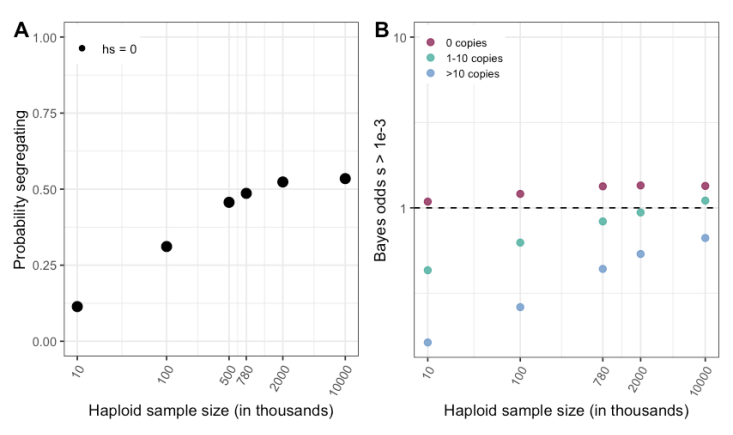
On a similar note, while a fixed hs simplifies much of the analysis, I wondered how results would differ for 1) completely recessive mutations and 2) under a distribution of dominance coefficients, especially one in which the most deleterious alleles were more recessive. Again, though I think it would strengthen the manuscript by no means do I feel this is a necessary addition, though some discussion of variation in dominance would be an easy and helpful add.
There's some discussion of population structure, but I also found myself wondering about GxE. That is, another reason a variant might be segregating is that it's conditionally neutral in some populations and only deleterious in a subset. I think no analysis to be done here, but perhaps some discussion?
We agree that our analysis ignores the possibilities of complete recessivity in fitness (h=0) as well as more complicated selection scenarios, such as spatially-varying selection (of the type that might be induced by GxE). We note however that so long as there are any fitness effects in heterozygotes, the allele dynamics will be primarily governed by hs; one might also imagine that under some conditions, the mean selection effect across environments would predict allele dynamics reasonably well even in the presence of GxE. Also worth exploring in our view is the standard assumption that hs remains fixed even as Ne changes dramatically. We now mention these points in the Outlook.
Maybe I missed it, but I don't think the acronym DNM is explained anywhere. While it was fairly self-explanatory, I did have a moment of wondering whether it was methylation or mutation and can't hurt to be explicit.
We apologize for the oversight and have updated the text accordingly.
Author Response:
Reviewer #1:
The manuscript by Piccolo and colleagues employs an in vitro neuruloid system to investigate the role of Hippo/YAP signaling pathway in early ectodermal fate specification. The authors examine YAP expression in forming neuruloids and test how manipulation of Hippo/Yap signaling affects their cellular composition. They observe that YAP expression is dynamic and enriched in cells occupying periphery of the neuruloid. Overactivation of the YAP activity by the Lats-kinase inhibitor TRULI leads to an expansion of TFAP2A+ cells (NNE) at early stages and of KRT18+ cells (epidermal) at later stages of development. Accordingly, the authors propose that YAP acts as a lineage determinant that (i) promotes a NNE fate during early development and (ii) impacts the fate of NNE cells by promoting an epidermal instead of a neural crest fate. Finally, the authors report that neuruloids developed with cells harboring mutations characteristics of Huntington's disease display elevated Yap activity.
The study takes advantage of the neuruloid system to examine the role of Hippo-Yap in early development and disease. A strength of the study is the use of the neuruloid as a proxy for the human embryo, which allows the authors to examine the control of spatial patterning in early development (in both wild type and altered cellular states). Yet, this model also presents significant limitations. Some of the results indicate a high degree of variability in YAP activity (and ectodermal patterning) in neuruloids obtained from different inductions. This raises the concern that the neuruloid system may interfere with Hippo/YAP. Furthermore, the model proposed by the authors is not consistent with the functional manipulations with pharmacological agents (e.g., pharmacological activation of YAP results in an increase of both neural and NNE cells; inhibition of YAP does not result in the expected phenotypes).
We thank the reviewer for her/his compliments on our work. The reviewer also points to the limitations of our neuruloid models and asks for clarifications.
The authors propose that YAP activation promotes a non-neural ectodermal (NNE) fate in early neuruloids, and subsequently drives NNE to differentiate into epidermis. However, manipulation of Hippo signaling with pharmacological inhibitors does not entirely support this, as treatment of neuruloids with agonist TRULI leads to expansion of both the PAX6 neural population and the NNE Tfap2a population. A prediction of the model is that treatment with verteporfin should neuralize the organoids, which is not the case (Fig 6A). This disconnect between the model presented in Figure 6D and the experimental results should be addressed by the authors.
We would like to thank the reviewer for this request. In our experiments we observed a dual effect of YAP activation (or HD mutation). As noted by the reviewer, ectodermal lineage- specification occurs both early (increased NNE induction) and late (enhanced epidermis differentiation and contraction of NC differentiation). Moreover, we observed a structural consequence of increased YAP activation in neuruloids, failure of the NE domain to fully close. Following the reviewer suggestion, we have now included an additional panel in Figure 6 to illustrate the phenotype alongside the difference in ectodermal lineage specification (panel E). We have also added in the Discussion a paragraph that highlights the architectural aspect of the observed phenotype.
Regarding the interpretation of the effect of pharmacological inhibition of YAP, we believe that the result of verteporfin treatment on WT neuruloids indicates that YAP activity is not required for this specification but can skew the differentiation towards NNE and epidermis. This is now included in the Results, and a new paragraph has been added in the Discussion directly addressing this point.
The study at times conflates YAP expression with activation of the Hippo-YAP pathway. While the images in figures 1,2, and 4 show changes in YAP expression, confirmation of Hippo-YAP pathway activity should include the use of a reporter (e.g., HOP-Flash) or at least high magnification images showing translocation of YAP to the nucleus. Overall, inclusion of better quantification of YAP-activity is crucial to support the manuscript's conclusions (the authors should also state the number of micropatterns used in each quantitative experiment).
Our evidence correlating YAP nuclear localization with activity is based on: (i) Immunoblots (Figures 1D and 2B); (ii) Confocal image analysis (Figures 1E, 2D, and 4B); and (iii) Induction of YAP target-genes expression as demonstrated by our scRNA-seq analysis, occurs in same epidermal (KRT18+) lineage cells that display the highest levels of YAP nuclear accumulation (Figure 2). However, to strengthen this argument and following the reviewer’s advice, we have now added magnified confocal microscope images of YAP/DAPI staining used to measure nuclear YAP localization at D4 (Figure 1—figure supplement 5). We have also added a slowed and magnified videos of the YAP-GFP/H2B-mCherry (and YAP-GFP alone) at D3-D4, which illustrates the dynamic accumulation of YAP in the nucleus of cells upon BMP4 stimulation (Figure 1—video 2, Figure 1—video 3, Figure 1—video 5, Figure 1—video 6, Figure 4—video 2 and Figure 4—video 3). Finally, the number of colonies analyzed for each experiment is now added in the Figure Legends.
A limitation of the study is that it does not investigate the possibility that Hippo/Yap could be affecting cell proliferation in the different lineages, instead of acting as a cell fate determinant. This is particularly important since Hippo is affected by cell density, which varies from the center to the periphery of the neuruloid. Different rates of proliferation over several days could potentially lead to drastic changes in neuruloid cellular composition.
To address the reviewer’s legitimate point, and assess to potential effects of YAP activation in HD-neuruloids, we performed three sets of experiments. First, we performed RNA-velocity analysis to determine the cellular trajectories within each lineage (FigureXA, below), and calculated the velocity of Seurat’s “cell cycle-associated” genes in each cell population in our scRNA-seq dataset at D4. This analysis indicates that the three ectodermal progenitors have a comparable rate of cell division, with NE being slightly faster than the others and epidermis being the slowest (Figure XB). However, these differences are subtle: the mean velocity of these cell-cycle genes within each population are not significantly different across the three ectodermal lineages (FigureXC). Second, comparison of velocity values between WT and HD, highlighted a significant HD-associated increase in the dynamic of cell-cycle associated genes only within the NE population (FigureXD), consistent with the observation that YAP is ectopically active in this lineage. This increase is also not very dramatic, for the mean velocity of these genes is not significantly different in any comparison at this time (Figure XE).
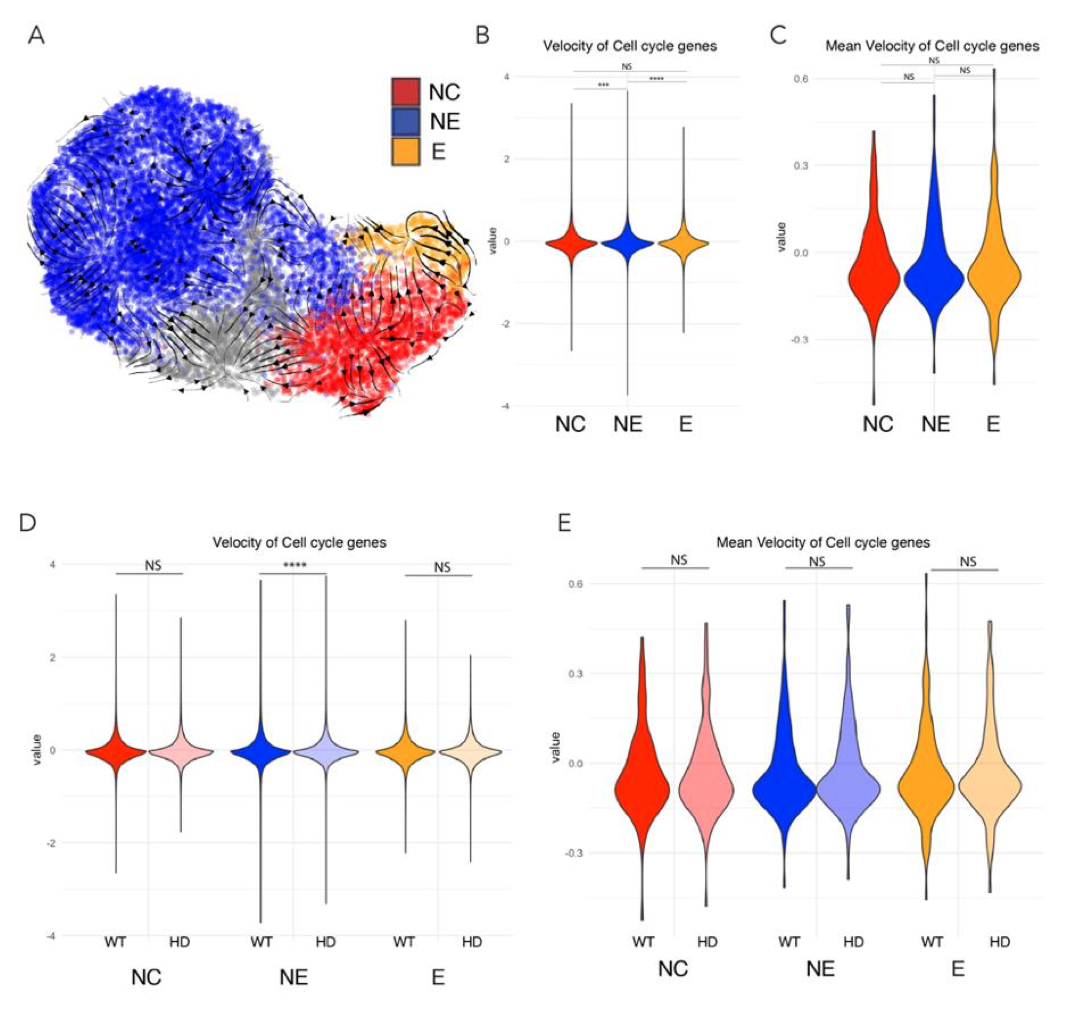
Figure X. Proliferation rate analysis of D4 neuruloid from scRNAseq dataset. A) transcriptional trajectories were identified in the three ectodermal lineages. B) Velocity of cell cycle associated genes show that NNE lineages (NC and E) are slightly faster than NE. C) However this is not significant the mean population level. D) NE in HD D4 neuruloids display subtle increase in the velocity of cell cycle associated genes. E) Such effect disappears at the mean population level.
Finally, quantification of the number of mitotic nuclei per colony as marked by phospho-histone H3 (Kim et al., 2017) at different time points, demonstrated that YAP activation by TRULI leads to an increase in cell proliferation, especially in late neuruloids. This evidence is now presented in the new Supplemental Figure 4—figure supplement 3. We thank the reviewer for bringing this point to our attention.
It is also important to note that our study does not suggest that YAP is a bona fide cell-fate determinant, but rather that that the global phenotypic signature of YAP activation is influenced by differential regulation of cell-cycle dynamics. Moreover, inasmuch as YAP inhibition with verteporfin does not effect neuruloid formation, we believe that YAP is more of a booster signal operating on top of differentiation programs.
The results of the study contradict a previous reports, and some of these contradictions are not sufficiently addressed. The authors state that the activation of YAP in culture leads to a "complete loss of NC-like SOX10+ colonies"; however, a number of studies in in vivo models support a role for YAP as a positive regulator of neural crest specification.
We thank the reviewer for pointing to the results observed in model systems. We have now included a paragraph in which we acknowledge that YAP has been previously associated with NC specification and survival. However, it should be noted that these conclusions are based on data obtained from non-human model organisms such as Xenopus, or relied on differentiation protocols that are independent of BMP4 stimulation. We believe that the phenotype of unbalanced specification of the NNE depends on an epistatic relationship between BMP4 and Hippo-YAP pathway, which might play a crucial role during human neurulation.
Furthermore, the authors briefly speculate on the finding that Huntington's disease neuruloids have high YAP activity (whereas tissues from patients have low activity), but there is no real clear link to the pathophysiology of the disease.
In our in vitro assay that recapitulates aspects of human neurulation, we observed an early increase (D4) followed by a later decline (D7) in YAP activity associated with HD mutation, which is comparable to a dysregulation of the Hippo pathway that was observed in HD patients. To better clarify this aspect and its potential implication during embryogenesis we have now expanded our Discussion on the possible connection between HD and embryonic development.
Experimental results presented in different figures are often inconsistent throughout the manuscript. This should be examined by the authors since it suggests a lack of reproducibility in the neuruloid protocol. For example, the expression of TFAP2A at D4 neuruloids is a sparse halo at D4 in Fig4D, but robust in Fig1E.
The reviewer is correct in pointing to a certain degree of variability between experiments, especially during the period (D4) when the first NNE lineage begin to emerge (i.e., Supplemental Figure 4—figure supplement 2). Because parallel experimental conditions such as comparison with HD samples or TRULI treatment show consistent trends, however, we believe that our interpretation of these results is fundamentally correct.
The western blot in fig1D shows bands for tYAP and pYAP at D4, while in Fig2B the bands are not present (Fig1D also shows double bands for both markers while fig2B presents single bands).
There are several splicing alternative isoforms of human YAP (Vrbský et al., 2021). Immunoblots for YAP in YAP-GFP biallelically tagged cell lines (Figure 1—figure supplement 1B) show that two isoforms are detectable at pluripotency. During neural induction (D1-D3) both isoforms are downregulated, and upon BMP4 stimulation the larger isoform (top band) is primarily upregulated, so that from D4 onwards only the top band is visible (Figure 2B). To better clarify this point, we now discuss this in the Results and include Supplemental Figures with the quantification of the top and bottom bands (D1-D4, Figure 1D) and only of the top band (D4D7, Figure 2B and Figure 1—figure supplement 4).
As Hippo responds very quickly to cell density, mechanical forces, etc., these inconsistencies could affect the proposed analyses.
As previously mentioned, we have assessed the effect on proliferation rate due to YAP activation by TRULI or HD mutation in neuruloids by scRNA-seq analysis and by counting the number of mitotic cells at different times. Our manuscript leaves open the relationship between HTT mutation and YAP hyperactivation, which likely is mediated in part by these factors, but we do address possible connections in the discussion.
Reviewer #2:
This manuscript by Piccolo et al identifies YAP signalling as key player in lineage determination during development of early human ectoderm. Additionally, the authors show that neuroloids generated using cells engineered to express penetrant levels of CAG repeats in the HTT gene display aberrant YAP signalling during ectodermal specification and that this phenotype can be partially rescued by inhibition of this pathway. This is interesting study and the similarity of the YAP-activated neuroloids and the HD neuroloids is striking. The value of this work would be increased by providing experiments to definitively demonstrate the role of YAP signalling in NNE specification and in HD neuroloids.
We also thank this reviewer for her/his compliments on our work. The reviewer also expresses specific recommendations listed below:
Specific comment: The authors describe the emergence of non-neuronal ectoderm (NNE) at the edges of the printed island cell colony and neuronal ectoderm (NE) within this circular colony. However, they do not show images of any lineage markers confirming that these regions are, in fact, NNE and NE.
We show in Figure 1E that the edges of the neuruloids are positive for TFAP2A, a marker for the NNE lineage. In Figure 4D we also show TFAP2A at the edge (NNE) and PAX6 at the center (NE). Additionally, the spatial identity of the various ectodermal lineages was full characterized in our previous study (Haremaki et al., 2018).
They also don't show that this YAP-GFP cell line recapitulates endogenous fix-and-stains of YAP in these colonies.
Figure 1E shows YAP expression at D4 by immunolabeling for YAP/DAPI acquired by confocal microscopy, which recapitulates that of immunofluorescence detection of nuclear YAP , shown in Figure 4B , and the results obtained by live fluorescence (YAP-GFP/H2B, Figure 4A).
Author Response
Reviewer #1 (Public Review):
The authors evaluate the involvement of the hippocampus in a fast-paced time-to-contact estimation task. They find that the hippocampus is sensitive to feedback received about accuracy on each trial and has activity that tracks behavioral improvement from trial to trial. Its activity is also related to a tendency for time estimation behavior to regress to the mean. This is a novel paradigm to explore hippocampal activity and the results are thus novel and important, but the framing as well as discussion about the meaning of the findings obscures the details of the results or stretches beyond them in many places, as detailed below.
We thank the reviewer for their constructive feedback and were happy to read that s/he considered our approach and results as novel and important. The comments led us to conduct new fMRI analyses, to clarify various unclear phrasings regarding our methods, and to carefully assess our framing of the interpretation and scope of our results. Please find our responses to the individual points below.
1) Some of the results appear in the posterior hippocampus and others in the anteriorhippocampus. The authors do not motivate predictions for anterior vs. posterior hippocampus, and they do not discuss differences found between these areas in the Discussion. The hippocampus is treated as a unitary structure carrying out learning and updating in this task, but the distinct areas involved motivate a more nuanced picture that acknowledges that the same populations of cells may not be carrying out the various discussed functions.
We thank the reviewer for pointing this out. We split the hippocampus into anterior and posterior sections because prior work suggested a different whole-brain connectivity and function of the two. This was mentioned in the methods section (page 15) in the initial submission but unfortunately not in the main text. Moreover, when discussing the results, we did indeed refer mostly to the hippocampus as a unitary structure for simplicity and readability, and because statements about subcomponents are true for the whole. However, we agree with the reviewer that the differences between anterior and posterior sections are very interesting, and that describing these effects in more detail might help to guide future work more precisely.
In response to the reviewer's comment, we therefore clarified at various locations throughout the manuscript whether the respective results were observed in the posterior or anterior section of the hippocampus, and we extended our discussion to reflect the idea that different functions may be carried out by distinct populations of hippocampal cells. In addition, we also now motivate the split into the different sections better in the main text. We made the following changes.
Page 3: “Second, we demonstrate that anterior hippocampal fMRI activity and functional connectivity tracks the behavioral feedback participants received in each trial, revealing a link between hippocampal processing and timing-task performance.
Page 3: “Fourth, we show that these updating signals in the posterior hippocampus were independent of the specific interval that was tested and activity in the anterior hippocampus reflected the magnitude of the behavioral regression effect in each trial.”
Page 5: “We performed both whole-brain voxel-wise analyses as well as regions-of-interest (ROI) analysis for anterior and posterior hippocampus separately, for which prior work suggested functional differences with respect to their contributions to memory-guided behavior (Poppenk et al., 2013, Strange et al. 2014).”
Page 9: “Because anterior and posterior sections of the hippocampus differ in whole-brain connectivity as well as in their contributions to memory-guided behavior (Strange et al. 2014), we analyzed the two sections separately. “
Page 9: “We found that anterior hippocampal activity as well as functional connectivity reflected the feedback participants received during this task, and its activity followed the performance improvements in a temporal-context-dependent manner. Its activity reflected trial-wise behavioral biases towards the mean of the sampled intervals, and activity in the posterior hippocampus signaled sensorimotor updating independent of the specific intervals tested.”
Page 10: “Intriguingly, the mechanisms at play may build on similar temporal coding principles as those discussed for motor timing (Yin & Troger, 2011; Eichenbaum, 2014; Howard, 2017; Palombo & Verfaellie, 2017; Nobre & van Ede, 2018; Paton & Buonomano, 2018; Bellmund et al., 2020, 2021; Shikano et al., 2021; Shimbo et al., 2021), with differential contributions of the anterior and posterior hippocampus. Note that our observation of distinct activity modulations in the anterior and posterior hippocampus suggests that the functions and coding principles discussed here may be mediated by at least partially distinct populations of hippocampal cells.”
Page 11: Interestingly, we observed that functional connectivity of the anterior hippocampus scaled negatively (Fig. 2C) with feedback valence [...]
2) Hippocampal activity is stronger for smaller errors, which makes the interpretationmore complex than the authors acknowledge. If the hippocampus is updating sensorimotor representations, why would its activity be lower when more updating is needed?
Indeed, we found that absolute (univariate) activity of the hippocampus scaled with feedback valence, the inverse of error (Fig. 2A). We see multiple possibilities for why this might be the case, and we discussed some of them in a dedicated discussion section (“The role of feedback in timed motor actions”). For example, prior work showed that hippocampal activity reflects behavioral feedback also in other tasks, which has been linked to learning (e.g. Schönberg et al., 2007; Cohen & Ranganath, 2007; Shohamy & Wagner, 2008; Foerde & Shohamy, 2011; Wimmer et al., 2012). In our understanding, sensorimotor updating is a form of ‘learning’ in an immediate and behaviorally adaptive manner, and we therefore consider our results well consistent with this earlier work. We agree with the reviewer that in principle activity should be stronger if there was stronger sensorimotor updating, but we acknowledge that this intuition builds on an assumption about the relationship between hippocampal neural activity and the BOLD signal, which is not entirely clear. For example, prior work revealed spatially informative negative BOLD responses in the hippocampus as a function of visual stimulation (e.g. Szinte & Knapen 2020), and the effects of inhibitory activity - a leading motif in the hippocampal circuitry - on fMRI data are not fully understood. This raises the possibility that the feedback modulation we observed might also involve negative BOLD responses, which would then translate to the observed negative correlation between feedback valence and the hippocampal fMRI signal, even if the magnitude of the underlying updating mechanism was positively correlated with error. This complicates the interpretation of the direction of the effect, which is why we chose to avoid making strong conclusions about it in our manuscript. Instead, we tried discussing our results in a way that was agnostic to the direction of the feedback modulation. Importantly, hippocampal connectivity with other regions did scale positively with error (Fig. 2B), which we again discussed in the dedicated discussion section.
In response to the reviewer’s comment, we revisited this section of our manuscript and felt the latter result deserved a better discussion. We therefore took this opportunity to extend our discussion of the connectivity results (including their relationship to the univariate-activity results as well as the direction of these effects), all while still avoiding strong conclusions about directionality. Following changes were made to the manuscript.
Page 11: Interestingly, we observed that functional connectivity of the anterior hippocampus scaled negatively (Fig. 2C) with feedback valence, unlike its absolute activity, which scaled positively with feedback valence (Fig. 2A,B), suggesting that the two measures may be sensitive to related but distinct processes.
Page 11: Such network-wide receptive-field re-scaling likely builds on a re-weighting of functional connections between neurons and regions, which may explain why anterior hippocampal connectivity correlated negatively with feedback valence in our data. Larger errors may have led to stronger re-scaling, which may be grounded in a corresponding change in functional connectivity.
3) Some tests were one-tailed without justification, which reduces confidence in the robustness of the results.
We thank the reviewer for pointing us to the fact that our choice of statistical tests was not always clear in the manuscript. In the analysis the reviewer is referring to, we predicted that stronger sensorimotor updating should lead to stronger activity as well as larger behavioral improvements across the respective trials. This is because a stronger update should translate to a more accurate “internal model” of the task and therefore to a better performance. We tested this one-sided hypothesis using the appropriate test statistic (contrasting trials in which behavioral performance did improve versus trials in which it did not improve), but we did not motivate our reasoning well enough in the manuscript. The revised manuscript therefore includes the two new statements shown below to motivate our choice of test statistic more clearly.
Page 7: [...] we contrasted trials in which participants had improved versus the ones in which they had not improved or got worse (see methods for details). Because stronger sensorimotor updating should lead to larger performance improvements, we predicted to find stronger activity for improvements vs. no improvements in these tests (one-tailed hypothesis).
Page 18: These two regressors reflect the tests for target-TTC-independent and target-TTC-specific updating, respectively. Because we predicted to find stronger activity for improvements vs. no improvements in behavioral performance, we here performed one-tailed statistical tests, consistent with the direction of this hypothesis. Improvement in performance was defined as receiving feedback of higher valence than in the corresponding previous trial.
4) The introduction motivates the novelty of this study based on the idea that thehippocampus has traditionally been thought to be involved in memory at the scale of days and weeks. However, as is partially acknowledged later in the Discussion, there is an enormous literature on hippocampal involvement in memory at a much shorter timescale (on the order of seconds). The novelty of this study is not in the timescale as much as in the sensorimotor nature of the task.
We thank the reviewer for this helpful suggestion. We agree that a key part of the novelty of this study is the use of the task that is typically used to study sensorimotor integration and timing rather than hippocampal processing, along with the new insights this task enabled about the role of the hippocampus in sensorimotor updating. As mentioned in the discussion, we also agree with the reviewer that there is prior literature linking hippocampal activity to mnemonic processing on short time scales. We therefore rephrased the corresponding section in the introduction to put more weight on the sensorimotor nature of our task instead of the time scales.
Note that the new statement still includes the time scale of the effects, but that it is less at the center of the argument anymore. We chose to keep it in because we do think that the majority of studies on hippocampal-dependent memory functions focus on longer time scales than our study does, and we expect that many readers will be surprised about the immediacy of how hippocampal activity relates to ongoing behavioral performance (on ultrashort time scales).
We changed the introduction to the following.
Page 2: Here, we approach this question with a new perspective by converging two parallel lines of research centered on sensorimotor timing and hippocampal-dependent cognitive mapping. Specifically, we test how the human hippocampus, an area often implicated in episodic-memory formation (Schiller et al., 2015; Eichenbaum, 2017), may support the flexible updating of sensorimotor representations in real time and in concert with other regions. Importantly, the hippocampus is not traditionally thought to support sensorimotor functions, and its contributions to memory formation are typically discussed for longer time scales (hours, days, weeks). Here, however, we characterize in detail the relationship between hippocampal activity and real-time behavioral performance in a fast-paced timing task, which is traditionally believed to be hippocampal-independent. We propose that the capacity of the hippocampus to encode statistical regularities of our environment (Doeller et al. 2005, Shapiro et al. 2017, Behrens et al., 2018; Momennejad, 2020; Whittington et al., 2020) situates it at the core of a brain-wide network balancing specificity vs. regularization in real time as the relevant behavior is performed.
5) The authors used three different regressors for the three feedback levels, asopposed to a parametric regressor indexing the level of feedback. The predictions are parametric, so a parametric regressor would be a better match, and would allow for the use of all the medium-accuracy data.
The reviewer raises a good point that overlaps with question 3 by reviewer 2. In the current analysis, we model the three feedback levels with three independent regressors (high, medium, low accuracy). We then contrast high vs. low accuracy feedback, obtaining the results shown in Fig. 2AB. The beta estimates obtained for medium-accuracy feedback are being ignored in this contrast. Following the reviewer’s feedback, we therefore re-run the model, this time modeling all three feedback levels in one parametric regressor. All other regressors in the model stayed the same. Instead of contrasting high vs. low accuracy feedback, we then performed voxel-wise t-tests on the beta estimates obtained for the parametric feedback regressor.
The results we observed were highly consistent across the two analyses, and all conclusions presented in the initial manuscript remain unchanged. While the exact t-scores differ slightly, we replicated the effects for all clusters on the voxel-wise map (on whole-brain FWE-corrected levels) as well as for the regions-of-interest analysis for anterior and posterior hippocampus. These results are presented in a new Supplementary Figure 3C.
Note that the new Supplementary Figure 3B shows another related new analyses we conducted in response to question 4 of reviewer 2. Here, we re-ran the initial analysis with three feedback regressors, but without modeling the inter-trial interval (ITI) and the inter-session interval (ISI, i.e. the breaks participants took) to avoid model over-specification. Again, we replicated the results for all clusters and the ROI analysis, showing that the initial results we presented are robust.
The following additions were made to the manuscript.
Page 5: Note that these results were robust even when fewer nuisance regressors were included to control for model over-specification (Fig. S3B; two-tailed one-sample t tests: anterior HPC, t(33) = -3.65, p = 8.9x10⁻⁴, pfwe = 0.002, d=-0.63, CI: [-1.01, -0.26]; posterior HPC, t(33) = -1.43, p = 0.161, pfwe = 0.322, d=-0.25, CI: [-0.59, 0.10]), and when all three feedback levels were modeled with one parametric regressors (Fig. S3C; two-tailed one-sample t tests: anterior HPC, t(33) = -3.59, p = 0.002, pfwe = 0.005, d=-0.56, CI: [-0.93, -0.20]; posterior HPC, t(33) = -0.99, p = 0.329, pfwe = 0.659, d=-0.17, CI: [-0.51, 0.17]). Further, there was no systematic relationship between subsequent trials on a behavioral level [...]
Page 17: Moreover, instead of modeling the three feedback levels with three independent regressors, we repeated the analysis modeling the three feedback levels as one parametric regressor with three levels. All other regressors remained unchanged, and the model included the regressors for ITIs and ISIs. We then conducted t-tests implemented in SPM12 using the beta estimates obtained for the parametric feedback regressor (Fig. 2C). Compared to the initial analyses presented above, this has the advantage that medium-accuracy feedback trials are considered for the statistics as well.
6) The authors claim that the results support the idea that the hippocampus is findingan "optimal trade-off between specificity and regularization". This seems overly speculative given the results presented.
We understand the reviewer's skepticism about this statement and agree that the manuscript does not show that the hippocampus is finding the trade-off between specificity and regularization. However, this is also not exactly what the manuscript claims. Instead, it suggests that the hippocampus “may contribute” to solving this trade-off (page 3) as part of a “brain-wide network“ (pages 2,3,9,12). We also state that “Our [...] results suggest that this trade-off [...] is governed by many regions, updating different types of task information in parallel” (Page 11). To us, these phrasings are not equivalent, because we do not think that the role of the hippocampus in sensorimotor updating (or in any process really) can be understood independently from the rest of the brain. We do however think that our results are in line with the idea that the hippocampus contributes to solving this trade-off, and that this is exciting and surprising given the sensorimotor nature of our task, the ultrashort time scale of the underlying process, and the relationship to behavioral performance. We tried expressing that some of the points discussed remain speculation, but it seems that we were not always successful in doing so in the initial submission. We apologize for the misunderstanding, adapted corresponding statements in the manuscript, and we express even more carefully that these ideas are speculation.
Following changes were made to the introduction and discussion.
Page 2: Here, we approach this question with a new perspective by converging two parallel lines of research centered on sensorimotor timing and hippocampal-dependent cognitive mapping. Specifically, we test how the human hippocampus, an area often implicated in episodic-memory formation (Schiller et al., 2015; Eichenbaum, 2017), may support the flexible updating of sensorimotor representations in real time and in concert with other regions.
Page 12: Because hippocampal activity (Julian & Doeller, 2020) and the regression effect (Jazayeri & Shadlen, 2010) were previously linked to the encoding of (temporal) context, we reasoned that hippocampal activity should also be related to the regression effect directly. This may explain why hippocampal activity reflected the magnitude of the regression effect as well as behavioral improvements independently from TTC, and why it reflected feedback, which informed the updating of the internal prior.
Page 12: This is in line with our behavioral results, showing that TTC-task performance became more optimal in the face of both of these two objectives. Over time, behavioral responses clustered more closely between the diagonal and the average line in the behavioral response profile (Fig. 1B, S1G), and the TTC error decreased over time. While different participants approached these optimal performance levels from different directions, either starting with good performance or strong regularization, the group approached overall optimal performance levels over the course of the experiment.
Page 13: This is in line with the notion that the hippocampus [...] supports finding an optimal trade off between specificity and regularization along with other regions. [...] Our results show that the hippocampus supports rapid and feedback-dependent updating of sensorimotor representations, suggesting that it is a central component of a brain-wide network balancing task specificity vs. regularization for flexible behavior in humans.
Note that in response to comment 1 by reviewer 2, the revised manuscript now reports the results of additional behavioral analyses that support the notion that participants find an optimal trade-off between specificity and regularization over time (independent of whether the hippocampus was involved or not).
7) The authors find that hippocampal activity is related to behavioral improvement fromthe prior trial. This seems to be a simple learning effect (participants can learn plenty about this task from a prior trial that does not have the exact same timing as the current trial) but is interpreted as sensitivity to temporal context. The temporal context framing seems too far removed from the analyses performed.
We agree with the reviewer that our observation that hippocampal activity reflects TTC-independent behavioral improvements across trials could have multiple explanations. Critically, i) one of them is that the hippocampus encodes temporal context, ii) it is only one of multiple observations that we build our interpretation on, and iii) our interpretation builds on multiple earlier reports
Interval estimates regress toward the mean of the sampled intervals, an effect that is often referred to as the “regression effect”. This effect, which we observed in our data too (Fig. 1B), has been proposed to reflect the encoding of temporal context (e.g. Jazayeri & Shadlen 2010). Moreover, there is a large body of literature on how the hippocampus may support the encoding of spatial and temporal context (e.g. see Bellmund, Polti & Doeller 2020 for review).
Because both hippocampal activity and the regression effect were linked to the encoding of (temporal) context, we reasoned that hippocampal activity should also be related to the regression effect directly. If so, one would expect that hippocampal activity should reflect behavioral improvements independently from TTC, it should reflect the magnitude of the regression effect, and it should generally reflect feedback, because it is the feedback that informs the updating of the internal prior.
All three observations may have independent explanations indeed, but they are all also in line with the idea that the hippocampus does encode temporal context and that this explains the relationship between hippocampal activity and the regression effect. It therefore reflects a sparse and reasonable explanation in our opinion, even though it necessarily remains an interpretation. Of course, we want to be clear on what our results are and what our interpretations are.
In response to the reviewer’s comment, we therefore toned down two of the statements that mention temporal context in the manuscript, and we removed an overly speculative statement from the result section. In addition, the discussion now describes more clearly how our results are in line with this interpretation.
Abstract: This is in line with the idea that the hippocampus supports the rapid encoding of temporal context even on short time scales in a behavior-dependent manner.
Page 13: This is in line with the notion that the hippocampus encodes temporal context in a behavior-dependent manner, and that it supports finding an optimal trade off between specificity and regularization along with other regions.
Page 12: Because hippocampal activity (Julian & Doeller, 2020) and the regression effect (Jazayeri & Shadlen, 2010) were previously linked to the encoding of (temporal) context, we reasoned that hippocampal activity should also be related to the regression effect directly. This may explain why hippocampal activity reflected the magnitude of the regression effect as well as behavioral improvements independently from TTC, and why it reflected feedback, which informed the updating of the internal prior.
The following statement was removed, overlapping with comment 2 by Reviewer 3:
Instead, these results are consistent with the notion that hippocampal activity signals the updating of task-relevant sensorimotor representations in real-time.
8) I am not sure the term "extraction of statistical regularities" is appropriate. The termis typically used for more complex forms of statistical relationships.
We agree with the reviewer that this expression may be interpreted differently by different readers and are grateful to be pointed to this fact. We therefore removed it and instead added the following (hopefully less ambiguous) statement to the manuscript.
Page 9: This study investigated how the human brain flexibly updates sensorimotor representations in a feedback-dependent manner in the service of timing behavior.
Reviewer #2 (Public Review):
The authors conducted a study involving functional magnetic resonance imaging and a time-to-contact estimation paradigm to investigate the contribution of the human hippocampus (HPC) to sensorimotor timing, with a particular focus on the involvement of this structure in specific vs. generalized learning. Suggestive of the former, it was found that HPC activity reflected time interval-specific improvements in performance while in support of the latter, HPC activity was also found to signal improvements in performance, which were not specific to the individual time intervals tested. Based on these findings, the authors suggest that the human HPC plays a key role in the statistical learning of temporal information as required in sensorimotor behaviour.
By considering two established functions of the HPC (i.e., temporal memory and generalization) in the context of a domain that is not typically associated with this structure (i.e., sensorimotor timing), this study is potentially important, offering novel insight into the involvement of the HPC in everyday behaviour. There is much to like about this submission: the manuscript is clearly written and well-crafted, the paradigm and analyses are well thought out and creative, the methodology is generally sound, and the reported findings push us to consider HPC function from a fresh perspective. A relative weakness of the paper is that it is not entirely clear to what extent the data, at least as currently reported, reflects the involvement of the HPC in specific and generalized learning. Since the authors' conclusions centre around this observation, clarifying this issue is, in my opinion, of primary importance.
We thank the reviewer for these positive and extremely helpful comments, which we will address in detail below. In response to these comments, the revised manuscript clarifies why the observed performance improvements are not at odds with the idea that an optimal trade-off between specificity and regularization is found, and how the time course of learning relates to those reported in previous literature. In addition, we conducted two new fMRI analyses, ensuring that our conclusions remain unchanged even if feedback is modeled with one parametric regressor, and if the number or nuisance regressors is reduced to control for overparameterization of the model. Please find our responses underneath each individual point below.
1) Throughout the manuscript, the authors discuss the trade-off between specific and generalized learning, and point towards Figure S1D as evidence for this (i.e., participants with higher TTC accuracy exhibited a weaker regression effect). What appears to be slightly at odds with this, however, is the observation that the deviation from true TTC decreased with time (Fig S1F) as the regression line slope approached 0.5 (Fig S1E) - one would have perhaps expected the opposite i.e., for deviation from true TTC to increase as generalization increases. To gain further insight into this, it would be helpful to see the deviation from true TTC plotted for each of the four TTC intervals separately and as a signed percentage of the target TTC interval (i.e., (+) or (-) deviation) rather than the absolute value.
We thank the reviewer for raising this important question and for the opportunity to elaborate on the relationship between the TTC error and the magnitude of the regression effect in behavior. Indeed, we see that the regression slopes approach 0.5 and that the TTC error decreases over the course of the experiment. We do not think that these two observations are at odds with each other for the following reasons:
First, while the reviewer is correct in pointing out that the deviation from the TTC should increase as “generalization increases”, that is not what we found. It was not the magnitude of the regularization per se that increased over time, but the overall task performance became more optimal in the face of both objectives: specificity and generalization. This optimum is at a regression-line slope of 0.5. Generalization (or regularization how we refer to it in the present manuscript), therefore did not increase per se on group level.
Second, the regression slopes approached 0.5 on the group-level, but the individual participants approached this level from different directions: Some of them started with a slope value close to 1 (high accuracy), whereas others started with a slope value close to 0 (near full regression to the mean). Irrespective of which slope value they started with, over time, they got closer to 0.5 (Rebuttal Figure 1A). This can also be seen in the fact that the group-level standard deviation in regression slopes becomes smaller over the course of the experiment (Rebuttal Figure 1B, SFig 1G). It is therefore not generally the case that the regression effect becomes stronger over time, but that it becomes more optimal for longer-term behavioral performance, which is then also reflected in an overall decrease in TTC error. Please see our response to the reviewer’s second comment for more discussion on this.
Third, the development of task performance is a function of two behavioral factors: a) the accuracy and b) the precision in TTC estimation. Accuracy describes how similar the participant’s TTC estimates were to the true TTC, whereas precision describes how similar the participant’s TTC estimates were relative to each other (across trials). Our results are a reflection of the fact that participants became both more accurate over time on average, but also more precise. To demonstrate this point visually, we now plotted the Precision and the Accuracy for the 8 task segments below (Rebuttal Figure 1C, SFig 1H), showing that both measures increased as the time progressed and more trials were performed. This was the case for all target durations.
In response to the reviewer’s comment, we clarified in the main text that these findings are not at odds with each other. Furthermore, we made clear that regularization per se did not increase over time on group level. We added additional supporting figures to the supplementary material to make this point. Note that in our view, these new analyses and changes more directly address the overall question the reviewer raised than the figure that was suggested, which is why we prioritized those in the manuscript.
However, we appreciated the suggestion a lot and added the corresponding figure for the sake of completeness.
Following additions were made.
Page 5: In support of this, participants' regression slopes converged over time towards the optimal value of 0.5, i.e. the slope value between veridical performance and the grand mean (Fig. S1F; linear mixed-effects model with task segment as a predictor and participants as the error term, F(1) = 8.172, p = 0.005, ε2=0.08, CI: [0.01, 0.18]), and participants' slope values became more similar (Fig. S1G; linear regression with task segment as predictor, F(1) = 6.283, p = 0.046, ε2 = 0.43, CI: [0, 1]). Consequently, this also led to an improvement in task performance over time on group level (i.e. task accuracy and precision increased (Fig. S1I), and the relationship between accuracy and precision became stronger (Fig. S1H), linear mixed-effect model results for accuracy: F(1) = 15.127, p = 1.3x10⁻⁴, ε2=0.06, CI: [0.02, 0.11], precision: F(1) = 20.189, p = 6.1x10⁻⁵, ε2 = 0.32, CI: [0.13, 1]), accuracy-precision relationship: F(1) = 8.288, p =0.036, ε2 = 0.56, CI: [0, 1], see methods for model details).
Page 12: This suggests that different regions encode distinct task regularities in parallel to form optimal sensorimotor representations to balance specificity and regularization. This is in line with our behavioral results, showing that TTC-task performance became more optimal in the face of both of these two objectives. Over time, behavioral responses clustered more closely between the diagonal and the average line in the behavioral response profile (Fig. 1B, S1G), and the TTC error decreased over time. While different participants approached these optimal performance levels from different directions, either starting with good performance or strong regularization, the group approached overall optimal performance levels over the course of the experiment.
Page 15: We also corroborated this effect by measuring the dispersion of slope values between participants across task segments using a linear regression model with task segment as a predictor and the standard deviation of slope values across participants as the dependent variable (Fig. S1G). As a measure of behavioral performance, we computed two variables for each target-TTC level: sensorimotor timing accuracy, defined as the absolute difference in estimated and true TTC, and sensorimotor timing precision, defined as coefficient of variation (standard deviation of estimated TTCs divided by the average estimated TTC). To study the interaction between these two variables for each target TTC over time, we first normalized accuracy by the average estimated TTC in order to make both variables comparable. We then used a linear mixed-effects model with precision as the dependent variable, task segment and normalized accuracy as predictors and target TTC as the error term. In addition, we tested whether accuracy and precision increased over the course of the experiment using separate linear mixed-effects models with task segment as predictor and participants as the error term.
2) Generalization relies on prior experience and can be relatively slow to develop as is the case with statistical learning. In Jazayeri and Shadlen (2010), for instance, learning a prior distribution of 11-time intervals demarcated by two briefly flashed cues (compared to 4 intervals associated with 24 possible movement trajectories in the current study) required ~500 trials. I find it somewhat surprising, therefore, that the regression line slope was already relatively close to 0.5 in the very first segment of the task. To what extent did the participants have exposure to the task and the target intervals prior to entering the scanner?
We thank the reviewer for raising the important question about the time course of learning in our task and how our results relate to prior work on this issue. Addressing the specific reviewer question first, participants practiced the task for 2-3 minutes prior to scanning. During the practice, they were not specifically instructed to perform the task as well as they could nor to encode the intervals, but rather to familiarize themselves with the general experimental setup and to ask potential questions outside the MRI machine. While they might have indeed started encoding the prior distribution of intervals during the practice already, we have no way of knowing, and we expect the contribution of this practice on the time course of learning during scanning to be negligible (for the reasons outlined above).
However, in addition to the specific question the reviewer asked, we feel that the comment raises two more general points: 1) How long does it take to learn the prior distribution of a set of intervals as a function of the number of intervals tested, and 2) Why are the learning slopes we report quite shallow already in the beginning of the scan?
Regarding (1), we are not aware of published reports that answer this question directly, and we expect that this will depend on the task that is used. Regarding the comparison to Jazayeri & Shadlen (2010), we believe the learning time course is difficult to compare between our study and theirs. As the reviewer mentioned, our study featured only 4 intervals compared to 11 in their work, based on which we would expect much faster learning in our task than in theirs. We did indeed sample 24 movement directions, but these were irrelevant in terms of learning the interval distribution. Moreover, unlike Jazayeri & Shadlen (2010), our task featured moving stimuli, which may have added additional sensory, motor and proprioceptive information in our study which the participants of the prior study could not rely on.
Regarding (2), and overlapping with the reviewer’s previous comment, the average learning slope in our study is indeed close to 0.5 already in the first task segment, but we would like to highlight that this is a group-level measure. The learning slopes of some subjects were closer to 1 (i.e. the diagonal in Fig 1B), and the one of others was closer to 0 (i.e. the mean) in the beginning of the experiment. The median slope was close to 0.65. Importantly, the slopes of most participants still approached 0.5 in the course of the experiment, and so did even the group-level slope the reviewer is referring to. This also means that participants’ slopes became more similar in the course of the experiment, and they approached 0.5, which we think reflects the optimal trade-off between regressing towards the mean and regressing towards the diagonal (in the data shown in Fig. 1B). This convergence onto the optimal trade-off value can be seen in many measures, including the mean slope (Rebuttal Figure 1A, SFig 1F), the standard deviation in slopes (Rebuttal Figure 1B, SFig 1G) as well as the Precision vs. Accuracy tradeoff (Rebuttal Figure 1C, SFig 1H). We therefore think that our results are well in line with prior literature, even though a direct comparison remains difficult due to differences in the task.
In response to the reviewer’s comment, and related to their first comment, we made the following addition to the discussion section.
Page 12: This suggests that different regions encode distinct task regularities in parallel to form optimal sensorimotor representations to balance specificity and regularization. This is well in line with our behavioral results, showing that TTC-task performance became more optimal in the face of both of these two objectives. Over time, behavioral responses clustered more closely between the diagonal and the average line in the behavioral response profile (Fig. 1B, S1G), and the TTC error decreased over time. While different participants approached these optimal performance levels from different directions, either starting with good performance or strong regularization, the group approached overall optimal performance levels over the course of the experiment.
3) I am curious to know whether differences between high-accuracy andmedium-accuracy feedback as well as between medium-accuracy and low-accuracy feedback predicted hippocampal activity in the first GLM analysis (middle page 5). Currently, the authors only present the findings for the contrast between high-accuracy and low-accuracy feedback. Examining all feedback levels may provide additional insight into the nature of hippocampal involvement and is perhaps more consistent with the subsequent GLM analysis (bottom page 6) in which, according to my understanding, all improvements across subsequent trials were considered (i.e., from low-accuracy to medium-accuracy; medium-accuracy to high-accuracy; as well as low-accuracy to high-accuracy).
We thank the reviewer for this thoughtful question, which relates to questions 5 by reviewer 1. The reviewer is correct that the contrast shown in Fig 2 does not consider the medium-accuracy feedback levels, and that the model in itself is slightly different from the one used in the subsequent analysis presented in Fig. 3. To reply to this comment as well as to a related one by reviewer 1 together, we therefore repeated the full analysis while modeling the three feedback levels in one parametric regressor, which includes the medium-accuracy feedback trials, and is consistent with the analysis shown in Fig. 3. The results of this new analysis are presented in the new Supplementary Fig. 3B.
In short, the model included one parametric regressor with three levels reflecting the three types of feedback, and all nuisance regressors remained unchanged. Instead of contrasting high vs. low accuracy feedback, we then performed voxel-wise t-tests on the beta estimates obtained for the parametric feedback regressor. We found that our results presented initially were very robust: Both the observed clusters in the voxel-wise analysis (on whole-brain FWE-corrected levels) as well as the ROI results replicated across the two analyses, and our conclusions therefore remain unchanged.
We made multiple textual additions to the manuscript to include this new analysis, and we present the results of the analysis including a direct comparison to our initial results in the new Supplementary Fig. 3. Following textual additions were.
Page 5: Note that these results were robust even when fewer nuisance regressors were included to control for model over-specification (Fig. S3B; two-tailed one-sample t tests: anterior HPC, t(33) = -3.65, p = 8.9x10⁻⁴, pfwe = 0.002, d=-0.63, CI: [-1.01, -0.26]; posterior HPC, t(33) = -1.43, p = 0.161, pfwe = 0.322, d=-0.25, CI: [-0.59, 0.10]), and when all three feedback levels were modeled with one parametric regressors (Fig. S3C; two-tailed one-sample t tests: anterior HPC, t(33) = -3.59, p = 0.002, pfwe = 0.005, d=-0.56, CI: [-0.93, -0.20]; posterior HPC, t(33) = -0.99, p = 0.329, pfwe = 0.659, d=-0.17, CI: [-0.51, 0.17]). Further, there was no systematic relationship between subsequent trials on a behavioral level [...]
Page 17: Moreover, instead of modeling the three feedback levels with three independent regressors, we repeated the analysis modeling the three feedback levels as one parametric regressor with three levels. All other regressors remained unchanged, and the model included the regressors for ITIs and ISIs. We then conducted t-tests implemented in SPM12 using thebeta estimates obtained for the parametric feedback regressor (Fig. S2C). Compared to the initial analyses presented above, this has the advantage that medium-accuracy feedback trials are considered for the statistics as well.
4) The authors modeled the inter-trial intervals and periods of rest in their univariateGLMs. This approach of modelling all 'down time' can lead to model over-specification and inaccurate parameter estimation (e.g. Pernet, 2014). A comment on this approach as well as consideration of not modelling the inter-trial intervals would be useful.
This is an important issue that we did not address in our initial manuscript. We are aware and agree with the reviewer’s general concern about model over-specification, which can be a big problem in regression as it leads to biased estimates. We did examine whether our model was overspecified before running it, but we did not report a formal test of it in the manuscript. We are grateful to be given the opportunity to do so now.
In response to the reviewer’s comment, we repeated the full analysis shown in Fig. 2 while excluding the nuisance regressors for inter-trial intervals (ISI) and breaks (or inter-session intervals, ISI). All other regressors and analysis steps stayed unchanged relative to the one reported in Fig. 2. The new results are presented in a new Supplementary Figure 3B.
Like for our previous analysis, we again see that the results we initially presented were extremely robust even on whole-brain FWE corrected levels, as well as on ROI level. Our conclusions therefore remain unchanged, and the results we presented initially are not affected by potential model overspecification. In addition to the new Supplementary Figure 3B, we made multiple textual changes to the manuscript to describe this new analysis and its implications. Note that we used the same nuisance regressors in all other GLM analyses too, meaning that it is also very unlikely that model overspecification affects any of the other results presented. We thank the reviewer for suggesting this analysis, and we feel including it in the manuscript has further strengthened the points we initially made.
Following additions were made to the manuscript.
Page 16: The GLM included three boxcar regressors modeling the feedback levels, one for ITIs, one for button presses and one for periods of rest (inter-session interval, ISI) [...]
Page 16: ITIs and ISIs were modeled to reduce task-unrelated noise, but to ensure that this did not lead to over-specification of the above-described GLM, we repeated the full analysis without modeling the two. All other regressors including the main feedback regressors of interest remained unchanged, and we repeated both the voxel-wise and ROI-wise statistical tests as described above (Fig. S2B).
Page 17: Note that these results were robust even when fewer nuisance regressors were included to control for model over-specification (Fig. S3B; two-tailed one-sample t tests: anterior HPC, t(33) = -3.65, p = 8.9x10⁻⁴, pfwe = 0.002, d=-0.63, CI: [-1.01, -0.26]; posterior HPC, t(33) = -1.43, p = 0.161, pfwe = 0.322, d=-0.25, CI: [-0.59, 0.10]), and when all three feedback levels were modeled with one parametric regressors (Fig. S3C; two-tailed one-sample t tests: anterior HPC, t(33) = -3.59, p = 0.002, pfwe = 0.005, d=-0.56, CI: [-0.93, -0.20]; posterior HPC, t(33) = -0.99, p = 0.329, pfwe = 0.659, d=-0.17, CI: [-0.51, 0.17]). Further, there was no systematic relationship between subsequent trials on a behavioral level [...]
Reviewer #3 (Public Review):
This paper reports the results of an interesting fMRI study examining the neural correlates of time estimation with an elegant design and a sensorimotor timing task. Results show that hippocampal activity and connectivity are modulated by performance on the task as well as the valence of the feedback provided. This study addresses a very important question in the field which relates to the function of the hippocampus in sensorimotor timing. However, a lack of clarity in the description of the MRI results (and associated methods) currently prevents the evaluation of the results and the interpretations made by the authors. Specifically, the model testing for timing-specific/timing-independent effects is questionable and needs to be clarified. In the current form, several conclusions appear to not be fully supported by the data.
We thank the reviewer for pointing us to many methodological points that needed clarification. We apologize for the confusion about our methods, which we clarify in the revised manuscript. Please find our responses to the individual points below.
Major points
Some methodological points lack clarity which makes it difficult to evaluate the results and the interpretation of the data.
We really appreciate the many constructive comments below. We feel that clarifying these points improved our manuscript immensely.
1) It is unclear how the 3 levels of accuracy and feedback (high, medium, and lowperformance) were computed. Please provide the performance range used for this classification. Was this adjusted to the participants' performance?
The formula that describes how the response window was computed for the different speed levels was reported in the methods section of the original manuscript on page 13. It reads as follows:
“The following formula was used to scale the response window width: d ± ((k ∗ d)/2) where d is the target TTC and k is a constant proportional to 0.3 and 0.6 for high and medium accuracy, respectively.“
In response to the reviewer’s comment, we now additionally report the exact ranges of the different response windows in a new Supplementary Table 1 and refer to it in the Methods section as follows.
Page 10: To calibrate performance feedback across different TTC durations, the precise response window widths of each feedback level scaled with the speed of the fixation target (Table S1).
2) The description of the MRI results lacks details. It is not always clear in the resultssection which models were used and whether parametric modulators were included or not in the model. This makes the results section difficult to follow. For example,
a) Figure 2: According to the description in the text, it appears that panels A and B report the results of a model with 3 regressors, ie one for each accuracy/feedback level (high, medium, low) without parametric modulators included. However, the figure legend for panel B mentions a parametric modulator suggesting that feedback was modelled for each trial as a parametric modulator. The distinction between these 2 models must be clarified in the result section.
We thank the reviewer very much for spotting this discrepancy. Indeed, Figure 2 shows the results obtained for a GLM in which we modeled the three feedback levels with separate regressors, not with one parametric regressor. Instead, the latter was the case for Figure 3. We apologize for the confusion and corrected the description in the figure caption, which now reads as follows. The description in the main text and the methods remain unchanged.
Caption Fig. 2: We plot the beta estimates obtained for the contrast between high vs. low feedback.
Moreover, note that in response to comment 5 by reviewer 1 and comment 3 by reviewer 2, the revised manuscript now additionally reports the results obtained for the parametric regressor in the new Supplementary Figure 3C. All conclusions remain unchanged.
Additionally, it is unclear how Figure 2A supports the following statement: "Moreover, the voxel-wise analysis revealed similar feedback-related activity in the thalamus and the striatum (Fig. 2A), and in the hippocampus when the feedback of the current trial was modeled (Fig. S3)." This is confusing as Figure 2A reports an opposite pattern of results between the striatum/thalamus and the hippocampus. It appears that the statement highlighted above is supported by results from a model including current trial feedback as a parametric modulator (reported in Figure S3).
We agree with the reviewer that our result description was confusing and changed it. It now reads as follows.
Page 5: Moreover, the voxel-wise analysis revealed feedback-related activity also in the thalamus and the striatum (Fig. 2A) [...]
Also, note that it is unclear from Figure 2A what is the direction of the contrast highlighting the hippocampal cluster (high vs. low according to the text but the figure shows negative values in the hippocampus and positive values in the thalamus). These discrepancies need to be addressed and the models used to support the statements made in the results sections need to be explicitly described.
The description of the contrast is correct. Negative values indicate smaller errors and therefore better feedback, which is mentioned in the caption of Fig. 2 as follows:
“Negative values indicate that smaller errors, and higher-accuracy feedback, led to stronger activity.”
Note that the timing error determined the feedback, and that we predicted stronger updating and therefore stronger activity for larger errors (similar to a prediction error). We found the opposite. We mention the reasoning behind this analysis at various locations in the manuscript e.g. when talking about the connectivity analysis:
“We reasoned that larger timing errors and therefore low-accuracy feedback would result in stronger updating compared to smaller timing errors and high-accuracy feedback”
In response to the reviewer’s remark, we clarified this further by adding the following statement to the result section.
Page 5: “Using a mass-univariate general linear model (GLM), we modeled the three feedback levels with one regressor each plus additional nuisance regressors (see methods for details). The three feedback levels (high, medium and low accuracy) corresponded to small, medium and large timing errors, respectively. We then contrasted the beta weights estimated for high-accuracy vs. low-accuracy feedback and examined the effects on group-level averaged across runs.”
b) Connectivity analyses: It is also unclear here which model was used in the PPIanalyses presented in Figure 2. As it appears that the seed region was extracted from a high vs. low contrast (without modulators), the PPI should be built using the same model. I assume this was the case as the authors mentioned "These co-fluctuations were stronger when participants performed poorly in the previous trial and therefore when they received low-accuracy feedback." if this refers to low vs. high contrast. Please clarify.
Yes, the PPI model was built using the same model. We clarified this in the methods section by adding the following statement to the PPI description.
Page 17: “The PPI model was built using the same model that revealed the main effects used to define the HPC sphere “
Yes, the reviewer is correct in thinking that the contrast shows the difference between low vs. high-accuracy feedback. We clarified this in the main text as well as in the caption of Fig. 2.
Caption Fig 2: [...] We plot results of a psychophysiological interactions (PPI) analysis conducted using the hippocampal peak effects in (A) as a seed for low vs. high-accuracy feedback. [...]
Page 17: The estimated beta weight corresponding to the interaction term was then tested against zero on the group-level using a t-test implemented in SPM12 (Fig. 2C). The contrast reflects the difference between low vs. high-accuracy feedback. This revealed brain areas whose activity was co-varying with the hippocampus seed ROI as a function of past-trial performance (n-1).
c) It is unclear why the model testing TTC-specific / TTC-independent effects (resultspresented in Figure 3) used 2 parametric modulators (as opposed to building two separate models with a different modulator each). I wonder how the authors dealt with the orthogonalization between parametric modulators with such a model. In SPM, the orthogonalization of parametric modulators is based on the order of the modulators in the design matrix. In this case, parametric modulator #2 would be orthogonalized to the preceding modulator so that a contrast focusing on the parametric modulator #2 would highlight any modulation that is above and beyond that explained by modulator #1. In this case, modulation of brain activity that is TTC-specific would have to be above and beyond a modulation that is TTC-independent to be highlighted. I am unsure that this is what the authors wanted to test here (or whether this is how the MRI design was built). Importantly, this might bias the interpretation of their results as - by design - it is less likely to observe TTC-specific modulations in the hippocampus as there is significant TTC-independent modulation. In other words, switching the order of the modulators in the model (or building two separate models) might yield different results. This is an important point to address as this might challenge the TTC-specific/TTC-independent results described in the manuscript.
We thank the reviewer for raising this important issue. When running the respective analysis, we made sure that the regressors were not collinear and we therefore did not expect substantial overlap in shared variance between them. However, we agree with the reviewer that orthogonalizing one regressor with respect to the other could still affect the results. To make sure that our expectations were indeed met, we therefore repeated the main analysis twice: 1) switching the order of the modulators and 2) turning orthogonalization off (which is possible in SPM12 unlike in previous versions). In all cases, our key results and conclusions remained unchanged, including the central results of the hippocampus analyses.
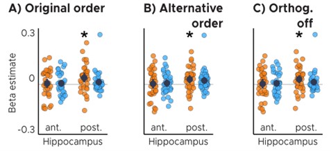
Anterior (ant.) / Posterior (post.) Hippocampus ROI analysis with A) original order of modulators, B) switching the order of the modulators and C) turning orthogonalization of modulators off. ABC) Orange color corresponds to the TTC-independent condition whereas light-blue color corresponds to the TTC-specific condition. Statistics reflect p<0.05 at Bonferroni corrected levels () obtained using a group-level one-tailed one-sample t-test against zero; A) pfwe = 0.017, B) pfwe = 0.039, C) pfwe = 0.039.*
Because orthogonalization did not affect the conclusions, the new manuscript simply reports the analysis for which it was turned off. Note that these new figures are extremely similar to the original figures we presented, which can be seen in the exemplary figure below showing our key results at a liberal threshold for transparency. In addition, we clarified that orthogonalization was turned off in the methods section as follows.
Page 18: These two regressors reflect the tests for target-TTC-independent and target-TTC-specific updating, respectively, and they were not orthogonalized to each other.
Comparison of old & new results: also see Fig. 3 and Fig. S5 in manuscript
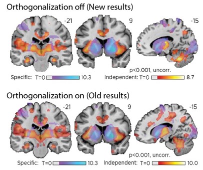
d) It is also unclear how the behavioral improvement was coded/classified "wecontrasted trials in which participants had improved versus the ones in which they had not improved or got worse"- It appears that improvement computation was based on the change of feedback valence (between high, medium and low). It is unclear why performance wasn't used instead? This would provide a finer-grained modulation?
We thank the reviewer for the opportunity to clarify this important point. First, we chose to model feedback because it is the feedback that determines whether participants update their “internal model” or not. Without feedback, they would not know how well they performed, and we would not expect to find activity related to sensorimotor updating. Second, behavioral performance and received feedback are tightly correlated, because the former determines the latter. We therefore do not expect to see major differences in results obtained between the two. Third, we did in fact model both feedback and performance in two independent GLMs, even though the way the results were reported in the initial submission made it difficult to compare the two.
Figure 4 shows the results obtained when modeling behavioral performance in the current trial as an F-contrast, and Supplementary Fig 4 shows the results when modeling the feedback received in the current trial as a t-contrast. While the voxel-wise t-maps/F-maps are also quite similar, we now additionally report the t-contrast for the behavioral-performance GLM in a new Supplementary Figure 4C. The t-maps obtained for these two different analyses are extremely similar, confirming that the direction of the effects as well as their interpretation remain independent of whether feedback or performance is modeled.
The revised manuscript refers to the new Supplementary Figure 4C as follows.
Page 17: In two independent GLMs, we analyzed the time courses of all voxels in the brain as a function of behavioral performance (i.e. TTC error) in each trial, and as a function of feedback received at the end of each trial. The models included one mean-centered parametric regressor per run, modeling either the TTC error or the three feedback levels in each trial, respectively. Note that the feedback itself was a function of TTC error in each trial [...] We estimated weights for all regressors and conducted a t-test against zero using SPM12 for our feedback and performance regressors of interest on the group level (Fig. S4A). [...]
Page 17: In addition to the voxel-wise whole-brain analyses described above, we conducted independent ROI analyses for the anterior and posterior sections of the hippocampus (Fig. S2A). Here, we tested the beta estimates obtained in our first-level analysis for the feedback and performance regressors of interest (Fig. S4B; two-tailed one-sample t tests: anterior HPC, t(33) = -5.92, p = 1.2x10⁻⁶, pfwe = 2.4x10⁻⁶, d=-1.02, CI: [-1.45, -0.6]; posterior HPC, t(33) = -4.07, p = 2.7x10⁻⁴, pfwe = 5.4x10⁻⁴, d=-0.7, CI: [-1.09, -0.32]). See section "Regions of interest definition and analysis" for more details.
If the feedback valence was used to classify trials as improved or not, how was this modelled (one regressor for improved, one for no improvement? As opposed to a parametric modulator with performance improvement?).
We apologize for the lack of clarity regarding our regressor design. In response to this comment, we adapted the corresponding paragraph in the methods to express more clearly that improvement trials and no-improvement trials were modeled with two separate parametric regressors - in line with the reviewer’s understanding. The new paragraph reads as follows.
Page 18: One regressor modeled the main effect of the trial and two parametric regressors modeled the following contrasts: Parametric regressor 1: trials in which behavioral performance improved \textit{vs}. parametric regressor 2: trials in which behavioral performance did not improve or got worse relative to the previous trial.
Last, it is also unclear how ITI was modelled as a regressor. Did the authors mean a parametric modulator here? Some clarification on the events modelled would also be helpful. What was the onset of a trial in the MRI design? The start of the trial? Then end? The onset of the prediction time?
The Inter-trial intervals (ITIs) were modeled as a boxcar regressor convolved with the hemodynamic response function. They describe the time after the feedback-phase offset and the subsequent trial onset. Moreover, the start of the trial was the moment when the visual-tracking target started moving after the ITI, whereas the trial end was the offset of the feedback phase (i.e. the moment in which the feedback disappeared from the screen). The onset of the “prediction time” was the moment in which the visual-tracking target stopped moving, prompting participants to estimate the time-to-contact. We now explain this more clearly in the methods as shown below.
Page 16: The GLM included three boxcar regressors modeling the feedback levels, one for ITIs, one for button presses and one for periods of rest (inter-session interval, ISI), which were all convolved with the canonical hemodynamic response function of SPM12. The start of the trial was considered as the trial onsets for modeling (i.e. the time when the visual-tracking target started moving). The trial end was the offset of the feedback phase (i.e. the moment in which the feedback disappeared from the screen). The ITI was the time between the offset of the feedback-phase and the subsequent trial onset.
On a related note, in response to question 4 by reviewer 2, we now repeated one of the main analyses (Fig. 2) without modeling the ITI (as well as the Inter-session interval, ISI). We found that our key results and conclusions are independent of whether or not these time points were modeled. These new results are presented in the new Supplementary Figure 3B.
Page 16: ITIs and ISIs were modeled to reduce task-unrelated noise, but to ensure that this did not lead to over-specification of the above-described GLM, we repeated the full analysis without modeling the two. [...]
- Perhaps as a result of a lack of clarity in the result section and the MRI methods, it appears that some conclusions presented in the result section are not supported by the data. E.g. "Instead, these results are consistent with the notion that hippocampal activity signals the updating of task-relevant sensorimotor representations in real-time." The data show that hippocampal activity is higher during and after an accurate trial. This pattern of results could be attributed to various processes such as e.g. reward or learning etc. I would recommend not providing such interpretations in the result section and addressing these points in the discussion.
Similar to above, statements like "These results suggest that the hippocampus updates information that is independent of the target TTC". The data show that higher hippocampal activity is linked to greater improvement across trials independent of the timing of the trial. The point about updating is rather speculative and should be presented in the discussion instead of the result section.
The reviewer is referring to two statements in the results section that reflect our interpretation rather than a description of the results. In response to the reviewer’s comment, we therefore removed the following statement from the results.
Instead, these results are consistent with the notion that hippocampal activity signals the updating of task-relevant sensorimotor representations in real-time.
In addition, we replaced the remaining statement by the following. We feel this new statement makes clear why we conducted the analysis that is described without offering an interpretation of the results that were presented before.
Page 8: We reasoned that updating TTC-independent information may support generalization performance by means of regularizing the encoded intervals based on the temporal context in which they were encoded.
Author Response:
Reviewer #1 (Public Review):
The manuscript provides very high quality single-cell physiology combined with population physiology to reveal distinctives roles for two anatomically dfferent LN populations in the cockroach antennal lobe. The conclusion that non-spiking LNs with graded responses show glomerular-restricted responses to odorants and spiking LNs show similar responses across glomeruli generally supported with strong and clean data, although the possibility of selective interglomerular inhibition has not been ruled out. On balance, the single-cell biophysics and physiology provides foundational information useful for well-grounded mechanistic understanding of how information is processed in insect antennal lobes, and how each LN class contributes to odor perception and behavior.
Thank you for this positive feedback.
Reviewer #2 (Public Review):
The manuscript "Task-specific roles of local interneurons for inter- and intraglomerular signaling in the insect antennal lobe" evaluates the spatial distribution of calcium signals evoked by odors in two major classes of olfactory local neurons (LNs) in the cockroach P. Americana, which are defined by their physiological and morphological properties. Spiking type I LNs have a patchy innervation pattern of a subset of glomeruli, whereas non-spiking type II LNs innervate almost all glomeruli (Type II). The authors' overall conclusion is that odors evoke calcium signals globally and relatively uniformly across glomeruli in type I spiking LNs, and LN neurites in each glomerulus are broadly tuned to odor. In contrast, the authors conclude that they observe odor-specific patterns of calcium signals in type II nonspiking LNs, and LN neurites in different glomeruli display distinct local odor tuning. Blockade of action potentials in type I LNs eliminates global calcium signaling and decorrelates glomerular tuning curves, converting their response profile to be more similar to that of type II LNs. From these conclusions, the authors infer a primary role of type I LNs in interglomerular signaling and type III LNs in intraglomerular signaling.
The question investigated by this study - to understand the computational significance of different types of LNs in olfactory circuits - is an important and significant problem. The design of the study is straightforward, but methodological and conceptual gaps raise some concerns about the authors' interpretation of their results. These can be broadly grouped into three main areas.
1) The comparison of the spatial (glomerular) pattern of odor-evoked calcium signals in type I versus type II LNs may not necessarily be a true apples-to-apples comparison. Odor-evoked calcium signals are an order of magnitude larger in type I versus type II cells, which will lead to a higher apparent correlation in type I cells. In type IIb cells, and type I cells with sodium channel blockade, odor-evoked calcium signals are much smaller, and the method of quantification of odor tuning (normalized area under the curve) is noisy. Compare, for instance, ROI 4 & 15 (Figure 4) or ROI 16 & 23 (Figure 5) which are pairs of ROIs that their quantification concludes have dramatically different odor tuning, but which visual inspection shows to be less convincing. The fact that glomerular tuning looks more correlated in type IIa cells, which have larger, more reliable responses compared to type IIb cells, also supports this concern.
We agree with the reviewer that "the comparison of the spatial (glomerular) pattern of odor-evoked calcium signals is not necessarily a true apples-to-apples comparison". Type I and type II LNs are different neuron types. Given their different physiology and morphology, this is not even close to a "true apples-to-apples comparison" - and a key point of the manuscript is to show just that.
As we have emphasized in response to Essential Revision 1, the differences in Ca2+ signals are not an experimental shortcoming but a physiologically relevant finding per se. These data, especially when combined with the electrophysiological data, contribute to a better understanding of these neurons’ physiological and computational properties.
It is physiologically determined that the Ca2+ signals during odorant stimulation in the type II LNs are smaller than in type I LNs. And yes, the signals are small because small postsynpathetic Ca2+ currents predominantly cause the signals. Regardless of the imaging method, this naturally reduces the signal-to-noise ratio, making it more challenging to detect signals. To address this issue, we used a well-defined and reproducible method for analyzing these signals. In this context, we do not agree with the very general criticism of the method. The reviewer questions whether the signals are odorant-induced or just noise (see also minor point 12). If we had recorded only noise, we would expect all tuning curves (for each odorant and glomerulus) to be the same. In this context, we disagree with the reviewer's statement that the tuning curves do not represent the Ca2+ signals in Figure 4 (ROI 4 and 15) and Figure 5 (ROI 16 and 23). This debate reflects precisely the kind of 'visual inspection bias' that our clearly defined analysis aims to avoid. On close inspection, the differences in Ca2+ signals can indeed be seen. Figure II (of this letter) shows the signals from the glomeruli in question at higher magnification. The sections of the recordings that were used for the tuning curves are marked in red.
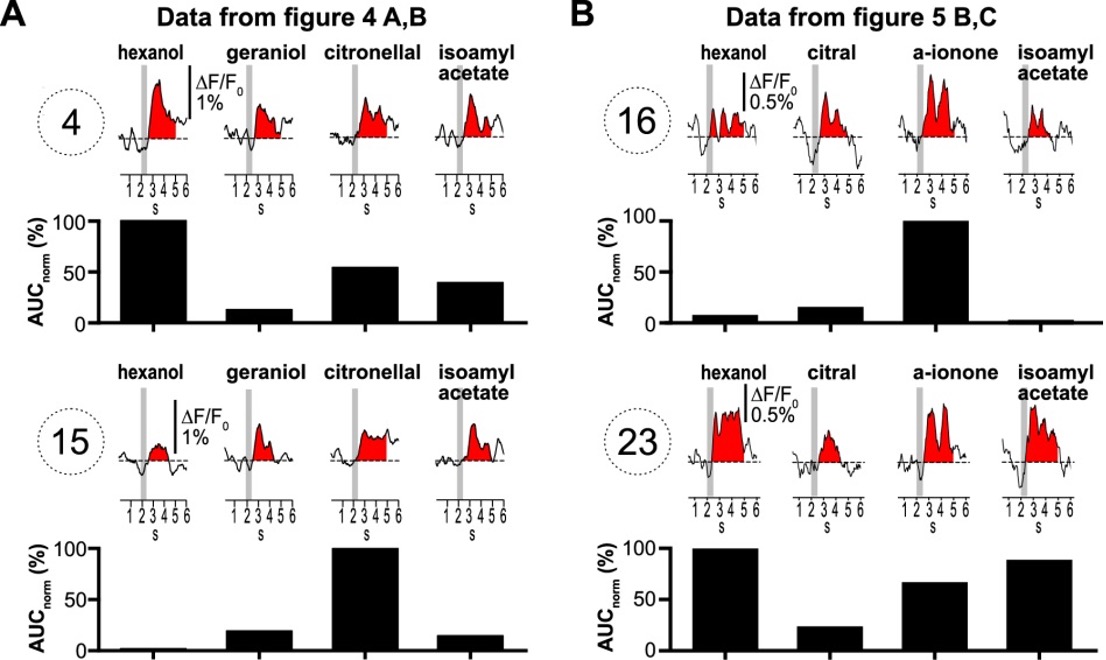
Figure II: Ca2+ signals of selected glomeruli that were questioned by the reviewer.
2) An additional methodological issue that compounds the first concern is that calcium signals are imaged with wide-field imaging, and signals from each ROI likely reflect out of plane signals. Out of plane artifacts will be larger for larger calcium signals, which may also make it impossible to resolve any glomerular-specific signals in the type I LNs.
Thank you for allowing us to clarify this point. The reviewer comment implies that the different amplitudes of the Ca2+ signals indicate some technical-methodological deficiency (poorly chosen odor concentration). But in fact, this is a key finding of this study that is physiologically relevant and crucial for understanding the function of the neurons studied. These very differences in the Ca2+ signals are evidence of the different roles these neurons play in AL. The different signal amplitudes directly show the distinct physiology and Ca2+ sources that dominate the Ca2+ signals in type I and type II LNs. Accordingly, it is impractical to equalize the magnitude of Ca2+ signals under physiological conditions by adjusting the concentration of odor stimuli.
In the following, we address these issues in more detail: 1) Imaging Method 2) Odorant stimulation 3) Cell type-specific Ca2+ signals
1) Imaging Method:
Of course, we agree with the reviewer comment that out-of-focus and out-of-glomerulus fluorescence can potentially affect measurements, especially in widefield optical imaging in thick tissue. This issue was carefully addressed in initial experiments. In type I LNs, which innervate a subset of glomeruli, we detected fluorescence signals, which matched the spike pattern of the electrophysiological recordings 1:1, only in the innervated glomeruli. In the not innervated ROIs (glomeruli), we detected no or comparatively very little fluorescence, even in glomeruli directly adjacent to innervated glomeruli.
To illustrate this, FIGURE I (of this response letter) shows measurements from an AL in which an uniglomerular projection neuron was investigated in an a set of experiments that were not directly related to the current study. In this experiment, a train of action potential was induced by depolarizing current. The traces show the action potential induced fluorescent signals from the innervated glomerulus (glomerulus #1) and the directly adjacent glomeruli.
These results do not entirely exclude that the large Ca2+ signals from the innervated LN glomeruli may include out-of-focus and out-of-glomerulus fluorescence, but they do show that the bulk of the signal is generated from the recorded neuron in the respective glomeruli.
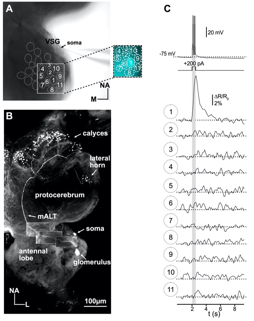
Figure I: Simultaneous electrophysiological and optophysiological recordings of a uniglomerular projection using the ratiometric Ca2+ indicator fura-2. The projection neuron has its arborization in glomerulus 1. The train of action potentials was induced with a depolarizing current pulse (grey bar).
2) Odorant Stimulation: It is important to note that the odorant concentration cannot be varied freely. For these experiments, the odorant concentrations have to be within a 'physiologically meaningful' range, which means: On the one hand, they have to be high enough to induce a clear response in the projection neurons (the antennal lobe output). On the other hand, however, the concentration was not allowed to be so high that the ORNs were stimulated nonspecifically. These criteria were met with the used concentrations since they induced clear and odorant-specific activity in projection neurons.
3) Cell type-specific Ca2+ signals:
The differences in Ca2+ signals are described and discussed in some detail throughout the text (e.g., page 6, lines 119-136; page 9, lines 193-198; page 10-11, lines 226-235; page 14-15, line 309-333). Briefly: In spiking type I LNs, the observed large Ca2+ signals are mediated mainly by voltage-depended Ca2+ channels activated by the Na+-driven action potential's strong depolarization. These large Ca2+ signals mask smaller signals that originate, for example, from excitatory synaptic input (i.e., evoked by ligand-activated Ca2+ conductances). Preventing the firing of action potentials can unmask the ligand-activated signals, as shown in Figure 4 (see also minor comments 8. and 10.). In nonspiking type II LNs, the action potential-generated Ca2+ signals are absent; accordingly, the Ca2+ signals are much smaller. In our model, the comparatively small Ca2+ signals in type II LNs are mediated mainly by (synaptic) ligand-gated Ca2+ conductances, possibly with contributions from voltage-gated Ca2+ channels activated by the comparatively small depolarization (compared with type I LNs).
Accordingly, our main conclusion, that spiking LNs play a primary role in interglomerular signaling, while nonspiking LNs play an essential role in intraglomeular signaling, can be DIRECTLY inferred from the differences in odorant induced Ca2+ signals alone.
a) Type I LN: The large, simultaneous, and uniform Ca2+ signals in the innervated glomeruli of an individual type I LN clearly show that they are triggered in each glomerulus by the propagated action potentials, which conclusively shows lateral interglomerular signal propagation.
b) Type II LNs: In the type II LNs, we observed relatively small Ca2+ signals in single glomeruli or a small fraction of glomeruli of a given neuron. Importantly, the time course and amplitude of the Ca2+ signals varied between different glomeruli and different odors. Considering that type II LNs in principle, can generate large voltage-activated Ca2+ currents (larger that type I LNS; page 4, lines 82-86, Husch et al. 2009a,b; Fusca and Kloppenburg 2021), these data suggest that in type II LNs electrical or Ca2+ signals spread only within the same glomerulus; and laterally only to glomeruli that are electrotonically close to the odorant stimulated glomerulus.
Taken together, this means that our conclusions regarding inter- and intraglomerular signaling can be derived from the simultaneously recorded amplitudes and the dynamics of the membrane potential and Ca2+ signals alone. This also means that although the correlation analyses support this conclusion nicely, the actual conclusion does not ultimately depend on the correlation analysis. We had (tried to) expressed this with the wording, “Quantitatively, this is reflected in the glomerulus-specific odorant responses and the diverse correlation coefficiiants across…” (page 10, lines 216-217) and “ …This is also reflected in the highly correlated tuning curves in type I LNs and low correlations between tuning curves in type II LNs”(page 13, lines 293-295).
3) Apart from the above methodological concerns, the authors' interpretation of these data as supporting inter- versus intra-glomerular signaling are not well supported. The odors used in the study are general odors that presumably excite feedforward input to many glomeruli. Since the glomerular source of excitation is not determined, it's not possible to assign the signals in type II LNs as arising locally - selective interglomerular signal propagation is entirely possible. Likewise, the study design does not allow the authors to rule out the possibility that significant intraglomerular inhibition may be mediated by type I LNs.
The reviewer addresses an important point. However, from the comment, we get the impression that he/she has not taken into account the entire data set and the DISCUSSION. In fact, this topic has already been discussed in some detail in the original version (page 12, lines 268-271; page 15-16; lines 358-374). This section even has a respective heading: "Inter- and intraglomerular signaling via nonspiking type II LNs" (page 15, line 338). We apologize if our explanations regarding this point were unclear, but we also feel that the reviewer is arguing against statements that we did not make in this way.
a) In 11 out of 18 type II LNs we found 'relatively uncorrelated' (r=0.43±0.16, N=11) glomerular tuning curves. These experiments argue strongly for a 'local excitation' with restricted signal propagation and do not provide support for interglomerular signal propagation. Thus, these results support our interpretation of intraglomerular signaling in this set of neurons.
b) In 7 out of 18 experiments, we observed 'higher correlated' glomerular tuning curves (r=0.78±0.07, N=7). We agree with the reviewer that this could be caused by various mechanisms, including simultaneous input to several glomeruli or by interglomerular signaling. Both possibilities were mentioned and discussed in the original version of the manuscript (page 12, lines 268-271; page 15-16; lines 358-374). In the Discussion, we considered the latter possibility in particular (but not exclusively) for the type IIa1 neurons that generate spikelets. Their comparatively stronger active membrane properties may be particularly suitable for selective signal transduction between glomeruli.
c) We have not ruled out that local signaling exists in type I LNs – in addition to interglomerular signaling. The highly localized Ca2+ signals in type I LNs, which we observed when Na+ -driven action potential generation was prevented, may support this interpretation. However, we would like to reiterate that the simultaneous electrophysiological and optophysiological recordings, which show highly correlated glomerular Ca2+ dynamics that match 1:1 with the simultaneously recorded action potential pattern, clearly suggest interglomerular signaling. We also want to emphasize that this interpretation is in agreement with previous models derived from electrophysiological studies(Assisi et al., 2011; Fujiwara et al., 2014; Hong and Wilson, 2015; Nagel and Wilson, 2016; Olsen and Wilson, 2008; Sachse and Galizia, 2002; Wilson, 2013).
In light of the reviewer's comment(s), we have modified the text to clarify these points (page 14, lines 317-319).
Reviewer #3 (Public Review):
To elucidate the role of the two types of LNs, the authors combined whole-cell patch clamp recordings with calcium imaging via single cell dye injection. This method enables to monitor calcium dynamics of the different axons and branches of single LNs in identified glomeruli of the antennal lobe, while the membrane potential can be recorded at the same time. The authors recorded in total from 23 spiking (type I LN) and 18 non-spiking (type II LN) neurons to a set of 9 odors and analyzed the firing pattern as well as calcium signals during odor stimulation for individual glomeruli. The recordings reveal on one side that odor-evoked calcium responses of type I LNs are odor-specific, but homogeneous across glomeruli and therefore highly correlated regarding the tuning curves. In contrast, odor-evoked responses of type II LNs show less correlated tuning patterns and rather specific odor-evoked calcium signals for each glomerulus. Moreover the authors demonstrate that both LN types exhibit distinct glomerular branching patterns, with type I innervating many, but not all glomeruli, while type II LNs branch in all glomeruli.
From these results and further experiments using pharmacological manipulation, the authors conclude that type I LNs rather play a role regarding interglomerular inhibition in form of lateral inhibition between different glomeruli, while type II LNs are involved in intraglomerular signaling by developing microcircuits in individual glomeruli.
In my opinion the methodological approach is quite challenging and all subsequent analyses have been carried out thoroughly. The obtained data are highly relevant, but provide rather an indirect proof regarding the distinct roles of the two LN types investigated. Nevertheless, the conclusions are convincing and the study generally represents a valuable and important contribution to our understanding of the neuronal mechanisms underlying odor processing in the insect antennal lobe. I think the authors should emphasize their take-home messages and resulting conclusions even stronger. They do a good job in explaining their results in their discussion, but need to improve and highlight the outcome and meaning of their individual experiments in their results section.
Thank you for this positive feedback.
References:
Assisi, C., Stopfer, M., Bazhenov, M., 2011. Using the structure of inhibitory networks to unravel mechanisms of spatiotemporal patterning. Neuron 69, 373–386. https://doi.org/10.1016/j.neuron.2010.12.019
Das, S., Trona, F., Khallaf, M.A., Schuh, E., Knaden, M., Hansson, B.S., Sachse, S., 2017. Electrical synapses mediate synergism between pheromone and food odors in Drosophila melanogaster . Proc Natl Acad Sci U S A 114, E9962–E9971. https://doi.org/10.1073/pnas.1712706114
Fujiwara, T., Kazawa, T., Haupt, S.S., Kanzaki, R., 2014. Postsynaptic odorant concentration dependent inhibition controls temporal properties of spike responses of projection neurons in the moth antennal lobe. PLOS ONE 9, e89132. https://doi.org/10.1371/journal.pone.0089132
Fusca, D., Husch, A., Baumann, A., Kloppenburg, P., 2013. Choline acetyltransferase-like immunoreactivity in a physiologically distinct subtype of olfactory nonspiking local interneurons in the cockroach (Periplaneta americana). J Comp Neurol 521, 3556–3569. https://doi.org/10.1002/cne.23371
Fuscà, D., and Kloppenburg, P. (2021). Odor processing in the cockroach antennal lobe-the network components. Cell Tissue Res.
Hong, E.J., Wilson, R.I., 2015. Simultaneous encoding of odors by channels with diverse sensitivity to inhibition. Neuron 85, 573–589. https://doi.org/10.1016/j.neuron.2014.12.040
Husch, A., Paehler, M., Fusca, D., Paeger, L., Kloppenburg, P., 2009a. Calcium current diversity in physiologically different local interneuron types of the antennal lobe. J Neurosci 29, 716–726. https://doi.org/10.1523/JNEUROSCI.3677-08.2009
Husch, A., Paehler, M., Fusca, D., Paeger, L., Kloppenburg, P., 2009b. Distinct electrophysiological properties in subtypes of nonspiking olfactory local interneurons correlate with their cell type-specific Ca2+ current profiles. J Neurophysiol 102, 2834–2845. https://doi.org/10.1152/jn.00627.2009
Nagel, K.I., Wilson, R.I., 2016. Mechanisms Underlying Population Response Dynamics in Inhibitory Interneurons of the Drosophila Antennal Lobe. J Neurosci 36, 4325–4338. https://doi.org/10.1523/JNEUROSCI.3887-15.2016
Neupert, S., Fusca, D., Kloppenburg, P., Predel, R., 2018. Analysis of single neurons by perforated patch clamp recordings and MALDI-TOF mass spectrometry. ACS Chem Neurosci 9, 2089–2096.
Olsen, S.R., Bhandawat, V., Wilson, R.I., 2007. Excitatory interactions between olfactory processing channels in the Drosophila antennal lobe. Neuron 54, 89–103. https://doi.org/10.1016/j.neuron.2007.03.010
Olsen, S.R., Wilson, R.I., 2008. Lateral presynaptic inhibition mediates gain control in an olfactory circuit. Nature 452, 956–960. https://doi.org/10.1038/nature06864
Sachse, S., Galizia, C., 2002. Role of inhibition for temporal and spatial odor representation in olfactory output neurons: a calcium imaging study. J Neurophysiol. 87, 1106–17.
Shang, Y., Claridge-Chang, A., Sjulson, L., Pypaert, M., Miesenbock, G., 2007. Excitatory Local Circuits and Their Implications for Olfactory Processing in the Fly Antennal Lobe. Cell 128, 601–612.
Wilson, R.I., 2013. Early olfactory processing in Drosophila: mechanisms and principles. Annu Rev Neurosci 36, 217–241. https://doi.org/10.1146/annurev-neuro-062111-150533
Yaksi, E., Wilson, R.I., 2010. Electrical coupling between olfactory glomeruli. Neuron 67, 1034–1047. https://doi.org/10.1016/j.neuron.2010.08.041
Author Response
Reviewer #1 (Public Review):
In computational modeling studies of behavioral data using reinforcement learning models, it has been implicitly assumed that parameter estimates generalize across tasks (generalizability) and that each parameter reflects a single cognitive function (interpretability). In this study, the authors examined the validity of these assumptions through a detailed analysis of experimental data across multiple tasks and age groups. The results showed that some parameters generalize across tasks, while others do not, and that interpretability is not sufficient for some parameters, suggesting that the interpretation of parameters needs to take into account the context of the task. Some researchers may have doubted the validity of these assumptions, but to my knowledge, no study has explicitly examined their validity. Therefore, I believe this research will make an important contribution to researchers who use computational modeling. In order to clarify the significance of this research, I would like the authors to consider the following points.
1) Effects of model misspecification
In general, model parameter estimates are influenced by model misspecification. Specifically, if components of the true process are not included in the model, the estimates of other parameters may be biased. The authors mentioned a little about model misspecification in the Discussion section, but they do not mention the possibility that the results of this study itself may be affected by it. I think this point should be discussed carefully.
The authors stated that they used state-of-the-art RL models, but this does not necessarily mean that the models are correctly specified. For example, it is known that if there is history dependence in the choice itself and it is not modeled properly, the learning rates depending on valence of outcomes (alpha+, alpha-) are subject to biases (Katahira, 2018, J Math Pscyhol). In the authors' study, the effect of one previous choice was included in the model as choice persistence, p. However, it has been pointed out that not including the effect of a choice made more than two trials ago in the model can also cause bias (Katahira, 2018). The authors showed taht the learning rate for positive RPE, alpha+ was inconsistent across tasks. But since choice persistence was included only in Task B, it is possible that the bias of alpha+ was different between tasks due to individual differences in choice persistence, and thus did not generalize.
However, I do not believe that it is necessary to perform a new analysis using the model described above. As for extending the model, I don't think it is possible to include all combinations of possible components. As is often said, every model is wrong, and only to varying degrees. What I would like to encourage the authors to do is to discuss such issues and then consider their position on the use of the present model. Even if the estimation results of this model are affected by misspecification, it is a fact that such a model is used in practice, and I think it is worthwhile to discuss the nature of the parameter estimates.
We thank the reviewer for this thoughtful question, and have added the following paragraph to the discussion section that is aims to address it:
“Another concern relates to potential model misspecification and its effects on model parameter estimates: If components of the true data-generating process are not included in a model (i.e., a model is misspecified), estimates of existing model parameters may be biased. For example, if choices have an outcome-independent history dependence that is not modeled properly, learning rate parameters have shown to be biased [63]. Indeed, we found that learning rate parameters were inconsistent across the tasks in our study, and two of our models (A and C) did not model history dependence in choice, while the third (model B) only included the effect of one previous choice (persistence parameter), but no multi-trial dependencies. It is hence possible that the differences in learning rate parameters between tasks were caused by differences in the bias induced by misspecification of history dependence, rather than a lack of generalization. Though pressing, however, this issue is difficult to resolve in practicality, because it is impossible to include all combinations of possible parameters in all computational models, i.e., to exhaustively search the space of possible models ("Every model is wrong, but to varying degrees"). Furthermore, even though our models were likely affected by some degree of misspecification, the research community is currently using models of this kind. Our study therefore sheds light on generalizability and interpretability in a realistic setting, which likely includes models with varying degrees of misspecification. Lastly, our models were fitted using robust computational tools and achieved good behavioral recovery (Fig. D.7), which also reduces the likelihood of model misspecification.“
2) Issue of reliability of parameter estimates
I think it is important to consider not only the bias in the parameter estimates, but also the issue of reliability, i.e., how stable the estimates will be when the same task is repeated with the same individual. For the task used in this study, has test-retest reliability been examined in previous studies? I think that parameters with low reliability will inevitably have low generalizability to other tasks. In this study, the use of three tasks seems to have addressed this issue without explicitly considering the reliability, but I would like the author to discuss this issue explicitly.
We thank the reviewer for this useful comment, and have added the following paragraph to the discussion section to address it:
“Furthermore, parameter generalizability is naturally bounded by parameter reliability, i.e., the stability of parameter estimates when participants perform the same task twice (test-retest reliability) or when estimating parameters from different subsets of the same dataset (split-half reliability). The reliability of RL models has recently become the focus of several parallel investigations [...], some employing very similar tasks to ours [...]. The investigations collectively suggest that excellent reliability can often be achieved with the right methods, most notably by using hierarchical model fitting. Reliability might still differ between tasks or models, potentially being lower for learning rates than other RL parameters [...], and differing between tasks (e.g., compare [...] to [...]). In this study, we used hierarchical fitting for tasks A and B and assessed a range of qualitative and quantitative measures of model fit for each task [...], boosting our confidence in high reliability of our parameter estimates, and the conclusion that the lack of between-task parameter correlations was not due to a lack of parameter reliability, but a lack of generalizability. This conclusion is further supported by the fact that larger between-task parameter correlations (r>0.5) than those observed in humans were attainable---using the same methods---in a simulated dataset with perfect generalization.“
3) About PCA
In this paper, principal component analysis (PCA) is used to extract common components from the parameter estimates and behavioral features across tasks. When performing PCA, were each parameter estimate and behavioral feature standardized so that the variance would be 1? There was no mention about this. It seems that otherwise the principal components would be loaded toward the features with larger variance. In addition, Moutoussis et al. (Neuron, 2021, 109 (12), 2025-2040) conducted a similar analysis of behavioral parameters of various decision-making tasks, but they used factor analysis instead of PCA. Although the authors briefly mentioned factor analysis, it would be better if they also mentioned the reason why they used PCA instead of factor analysis, which can consider unique variances.
To answer the reviewer's first question: We indeed standardized all features before performing the PCA. Apologies for missing to include this information - we have now added a corresponding sentence to the methods sections.
We also thank the reviewer for the mentioned reference, which is very relevant to our findings and can help explain the roles of different PCs. Like in our study, Moutoussis et al. found a first PC that captured variability in task performance, and subsequent PCs that captured task contrasts. We added the following paragraph to our manuscript:
“PC1 therefore captured a range of "good", task-engaged behaviors, likely related to the construct of "decision acuity" [...]. Like our PC1, decision acuity was the first component of a factor analysis (variant of PCA) conducted on 32 decision-making measures on 830 young people, and separated good and bad performance indices. Decision acuity reflects generic decision-making ability, and predicted mental health factors, was reflected in resting-state functional connectivity, but was distinct from IQ [...].”
To answer the reviewer's question about PCA versus FA, both approaches are relatively similar conceptually, and oftentimes share the majority of the analysis pipeline in practice. The main difference is that PCA breaks up the existing variance in a dataset in a new way (based on PCs rather than the original data features), whereas FA aims to identify an underlying model of latent factors that explain the observable features. This means that PCs are linear combinations of the original data features, whereas Factors are latent factors that give rise to the observable features of the dataset with some noise, i.e., including an additional error term.
However, in practice, both methods share the majority of computation in the way they are implemented in most standard statistical packages: FA is usually performed by conducting a PCA and then rotating the resulting solution, most commonly using the Varimax rotation, which maximizes the variance between features loadings on each factor in order to make the result more interpretable, and thereby foregoing the optimal solution that has been achieved by the PCA (which lack the error term). Maximum variance in feature loadings means that as many features as possible will have loadings close to 0 and 1 on each factor, reducing the number of features that need to be taken into account when interpreting this factor. Most relevant in our situation is that PCA is usually a special case of FA, with the only difference that the solution is not rotated for maximum interpretability. (Note that this rotation can be minor if feature loadings already show large variance in the PCA solution.)
To determine how much our results would change in practice if we used FA instead of PCA, we repeated the analysis using FA. Both are shown side-by-side below, and the results are quite similar:
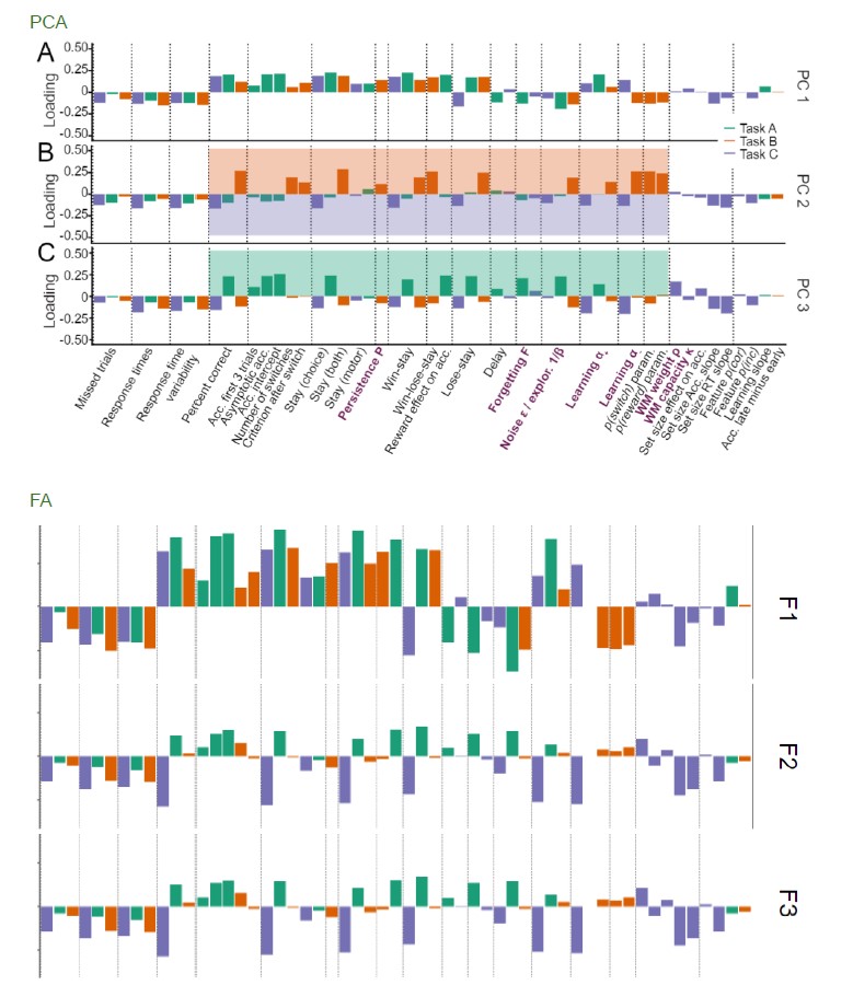
We therefore conclude that our specific results are robust to the choice of method used, and that there is reason to believe that our PC1 is related to Moutoussis et al.’s F1 despite the differences in method.
Reviewer #2 (Public Review):
I am enthusiastic about the comprehensive approach, the thorough analysis, and the intriguing findings. This work makes a timely contribution to the field and warrants a wider discussion in the community about how computational methods are deployed and interpreted. The paper is also a great and rare example of how much can be learned from going beyond a meta-analytic approach to systematically collect data that assess commonly held assumptions in the field, in this case in a large data-driven study across multiple tasks. My only criticism is that at times, the paper misses opportunities to be more constructive in pinning down exactly why authors observe inconsistencies in parameter fits and interpretation. And the somewhat pessimistic outlook relies on some results that are, in my view at least, somewhat expected based on what we know about human RL. Below I summarize the major ways in which the paper's conclusions could be strengthened.
One key point the authors make concerns the generalizability of absolute vs. relative parameter values. It seems that at least in the parameter space defined by +LRs and exploration/noise (which are known to be mathematically coupled), subjects clustered similarly for tasks A and C. In other words, as the authors state, "both learning rate and inverse temperature generalized in terms of the relationships they captured between participants". This struck me as a more positive and important result than it was made out to be in the paper, for several reasons:
- As authors point out in the discussion, a large literature on variable LRs has shown that people adapt their learning rates trial-by-trial to the reward function of the environment; given this, and given that all models tested in this work have fixed learning rates, while the three tasks vary on the reward function, the comparison of absolute values seems a bit like a red-herring.
We thank the reviewers for this recommendation and have reworked the paper substantially to address the issue. We have modified the highlights, abstract, introduction, discussion, conclusion, and relevant parts of the results section to provide equal weight to the successes and failures of generalization.
Highlights:
● “RL decision noise/exploration parameters generalize in terms of between-participant variation, showing similar age trajectories across tasks.”
● “These findings are in accordance with previous claims about the developmental trajectory of decision noise/exploration parameters.”
Abstract:
● “We found that some parameters (exploration / decision noise) showed significant generalization: they followed similar developmental trajectories, and were reciprocally predictive between tasks.“
The introduction now introduces different potential outcomes of our study with more equal weight:
“Computational modeling enables researchers to condense rich behavioral datasets into simple, falsifiable models (e.g., RL) and fitted model parameters (e.g., learning rate, decision temperature) [...]. These models and parameters are often interpreted as a reflection of ("window into") cognitive and/or neural processes, with the ability to dissect these processes into specific, unique components, and to measure participants' inherent characteristics along these components.
For example, RL models have been praised for their ability to separate the decision making process into value updating and choice selection stages, allowing for the separate investigation of each dimension. Crucially, many current research practices are firmly based on these (often implicit) assumptions, which give rise to the expectation that parameters have a task- and model-independent interpretation and will seamlessly generalize between studies. However, there is growing---though indirect---evidence that these assumptions might not (or not always) be valid.
The following section lays out existing evidence in favor and in opposition of model generalizability and interpretability. Building on our previous opinion piece, which---based on a review of published studies---argued that there is less evidence for model generalizability and interpretability than expected based on current research practices [...], this study seeks to directly address the matter empirically.”
We now also provide more even evidence for both potential outcomes:
“Many current research practices are implicitly based on the interpretability and generalizability of computational model parameters (despite the fact that many researchers explicitly distance themselves from these assumptions). For our purposes, we define a model variable (e.g., fitted parameter, reward-prediction error) as generalizable if it is consistent across uses, such that a person would be characterized with the same values independent of the specific model or task used to estimate the variable. Generalizability is a consequence of the assumption that parameters are intrinsic to participants rather than task dependent (e.g., a high learning rate is a personal characteristic that might reflect an individual's unique brain structure). One example of our implicit assumptions about generalizability is the fact that we often directly compare model parameters between studies---e.g., comparing our findings related to learning-rate parameters to a previous study's findings related to learning-rate parameters. Note that such a comparison is only valid if parameters capture the same underlying constructs across studies, tasks, and model variations, i.e., if parameters generalize. The literature has implicitly equated parameters in this way in review articles [...], meta-analyses [...], and also most empirical papers, by relating parameter-specific findings across studies. We also implicitly evoke parameter generalizability when we study task-independent empirical parameter priors [...], or task-independent parameter relationships (e.g., interplay between different kinds of learning rates [...]), because we presuppose that parameter settings are inherent to participants, rather than task specific.
We define a model variable as interpretable if it isolates specific and unique cognitive elements, and/or is implemented in separable and unique neural substrates. Interpretability follows from the assumption that the decomposition of behavior into model parameters "carves cognition at its joints", and provides fundamental, meaningful, and factual components (e.g., separating value updating from decision making). We implicitly invoke interpretability when we tie model variables to neural substrates in a task-general way (e.g., reward prediction errors to dopamine function [...]), or when we use parameters as markers of psychiatric conditions (e.g., working-memory parameter and schizophrenia [...]). Interpretability is also required when we relate abstract parameters to aspects of real-world decision making [...], and generally, when we assume that model variables are particularly "theoretically meaningful" [...].
However, in midst the growing recognition of computational modeling, the focus has also shifted toward inconsistencies and apparent contradictions in the emerging literature, which are becoming apparent in cognitive [...], developmental [...], clinical [...], and neuroscience studies [...], and have recently become the focus of targeted investigations [...]. For example, some developmental studies have shown that learning rates increased with age [...], whereas others have shown that they decrease [...]. Yet others have reported U-shaped trajectories with either peaks [...] or troughs [...] during adolescence, or stability within this age range [...] (for a comprehensive review, see [...]; for specific examples, see [...]). This is just one striking example of inconsistencies in the cognitive modeling literature, and many more exist [...]. These inconsistencies could signify that computational modeling is fundamentally flawed or inappropriate to answer our research questions. Alternatively, inconsistencies could signify that the method is valid, but our current implementations are inappropriate [...]. However, we hypothesize that inconsistencies can also arise for a third reason: Even if both method and implementation are appropriate, inconsistencies like the ones above are expected---and not a sign of failure---if implicit assumptions of generalizability and interpretability are not always valid. For example, model parameters might be more context-dependent and less person-specific that we often appreciate [...]“
In the results section, we now highlight findings more that are compatible with generalization: “For α+, adding task as a predictor did not improve model fit, suggesting that α+ showed similar age trajectories across tasks (Table 2). Indeed, α+ showed a linear increase that tapered off with age in all tasks (linear increase: task A: β = 0.33, p < 0.001; task B: β = 0.052, p < 0.001; task C: β = 0.28, p < 0.001; quadratic modulation: task A: β = −0.007, p < 0.001; task B: β = −0.001, p < 0.001; task C: β = −0.006, p < 0.001). For noise/exploration and Forgetting parameters, adding task as a predictor also did not improve model fit (Table 2), suggesting similar age trajectories across tasks.”
“For both α+ and noise/exploration parameters, task A predicted tasks B and C, and tasks B and C predicted task A, but tasks B and C did not predict each other (Table 4; Fig. 2D), reminiscent of the correlation results that suggested successful generalization (section 2.1.2).”
“Noise/exploration and α+ showed similar age trajectories (Fig. 2C) in tasks that were sufficiently similar (Fig. 2D).” And with respect to our simulation analysis (for details, see next section):
“These results show that our method reliably detected parameter generalization in a dataset that exhibited generalization. ”
We also now provide more nuance in our discussion of the findings:
“Both generalizability [...] and interpretability (i.e., the inherent "meaningfulness" of parameters) [...] have been explicitly stated as advantages of computational modeling, and many implicit research practices (e.g., comparing parameter-specific findings between studies) showcase our conviction in them [...]. However, RL model generalizability and interpretability has so far eluded investigation, and growing inconsistencies in the literature potentially cast doubt on these assumptions. It is hence unclear whether, to what degree, and under which circumstances we should assume generalizability and interpretability. Our developmental, within-participant study revealed a nuanced picture: Generalizability and interpretability differed from each other, between parameters, and between tasks.”
“Exploration/noise parameters showed considerable generalizability in the form of correlated variance and age trajectories. Furthermore, the decline in exploration/noise we observed between ages 8-17 was consistent with previous studies [13, 66, 67], revealing consistency across tasks, models, and research groups that supports the generalizability of exploration / noise parameters. However, for 2/3 pairs of tasks, the degree of generalization was significantly below the level of generalization expected for perfect generalization. Interpretability of exploration / noise parameters was mixed: Despite evidence for specificity in some cases (overlap in parameter variance between tasks), it was missing in others (lack of overlap), and crucially, parameters lacked distinctiveness (substantial overlap in variance with other parameters).”
“Taken together, our study confirms the patterns of generalizable exploration/noise parameters and task-specific learning rate parameters that are emerging from the literature [13].”
- Regarding the relative inferred values, it's unclear how high we really expect correlations between the same parameter across tasks to be. E.g., if we take Task A and make a second, hypothetical, Task B by varying one feature at a time (say, stochasticity in reward function), how correlated are the fitted LRs going to be? Given the different sources of noise in the generative model of each task and in participant behavior, it is hard to know whether a correlation coefficient of 0.2 is "good enough" generalizability.
We thank the reviewer for this excellent suggestion, which we think helped answer a central question that our previous analyses had failed to address, and also provided answers to several other concerns raised by both reviewers in other section. We have conducted these additional analyses as suggested, simulating artificial behavioral data for each task, fitting these data using the models used in humans, repeating the analyses performed on humans on the new fitted parameters, and using bootstrapping to statistically compare humans to the hence obtained ceiling of generalization. We have added the following section to our paper, which describes the results in detail:
“Our analyses so far suggest that some parameters did not generalize between tasks, given differences in age trajectories (section 2.1.3) and a lack of mutual prediction (section 2.1.4). However, the lack of correspondence could also arise due to other factors, including behavioral noise, noise in parameter fitting, and parameter trade-offs within tasks. To rule these out, we next established the ceiling of generalizability attainable using our method.
We established the ceiling in the following way: We first created a dataset with perfect generalizability, simulating behavior from agents that use the same parameters across all tasks (suppl. Appendix E). We then fitted this dataset in the same way as the human dataset (e.g., using the same models), and performed the same analyses on the fitted parameters, including an assessment of age trajectories (suppl. Table E.8) and prediction between tasks (suppl. Tables E.9, E.10, and E.11). These results provide the practical ceiling of generalizability. We then compared the human results to this ceiling to ensure that the apparent lack of generalization was valid (significant difference between humans and ceiling), and not in accordance with generalization (lack of difference between humans and ceiling).
Whereas humans had shown divergent trajectories for parameter alpha- (Fig. 2B; Table 1), the simulated agents did not show task differences for alpha- or any other parameter (suppl. Fig E.8B; suppl. Table E.8, even when controlling for age (suppl. Tables E.9 and E.10), as expected from a dataset of generalizing agents. Furthermore, the same parameters were predictive between tasks in all cases (suppl. Table E.11). These results show that our method reliably detected parameter generalization in a dataset that exhibited generalization.
Lastly, we established whether the degree of generalization in humans was significantly different from agents. To this aim, we calculated the Spearman correlations between each pair of tasks for each parameter, for both humans (section 2.1.2; suppl. Fig. H.9) and agents, and compared both using bootstrapped confidence intervals (suppl. Appendix E). Human parameter correlations were significantly below the ceiling for all parameters except alpha+ (A vs B) and epsilon / 1/beta (A vs C; suppl. Fig. E.8C). This suggests that humans were within the range of maximally detectable generalization in two cases, but showed less-than-perfect generalization between other task combinations and for parameters Forgetting and alpha-.”
- The +LR/inverse temp relationship seems to generalize best between tasks A/C, but not B/C, a common theme in the paper. This does not seem surprising given that in A and C there is a key additional task feature over the bandit task in B -- which is the need to retain state-action associations. Whether captured via F (forgetting) or K (WM capacity), the cognitive processes involved in this learning might interact with LR/exploration in a different way than in a task where this may not be necessary.
We thank the reviewer for this comment, which raises an important issue. We are adding the specific pairwise correlations and scatter plots for the pairs of parameters the reviewer asked about below (“bf_alpha” = LR task A; “bf_forget” = F task A; “rl_forget” = F task C; “rl_log_alpha” = LR task C; “rl_K” = WM capacity task C):
Within tasks:
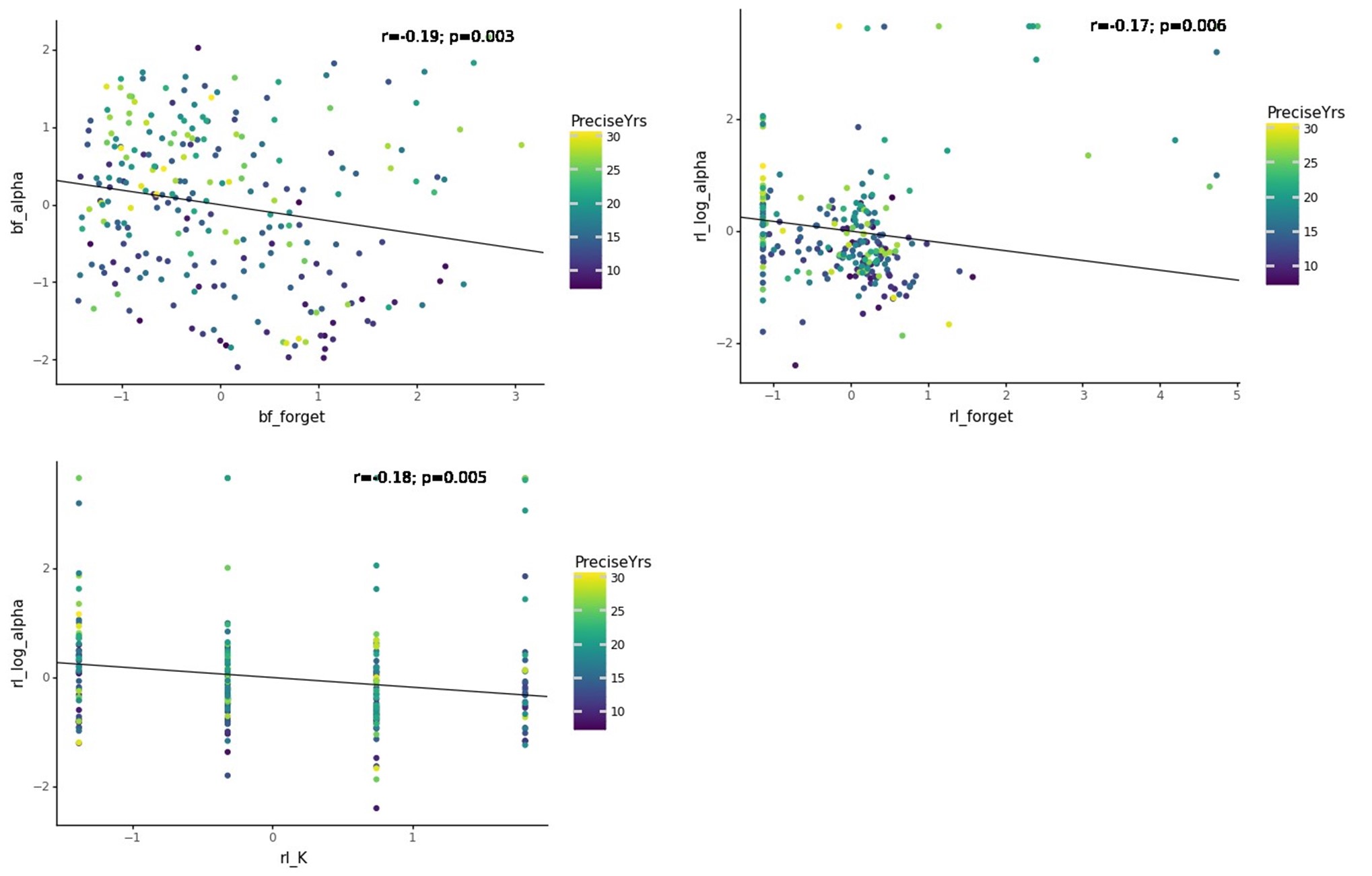
Between tasks:
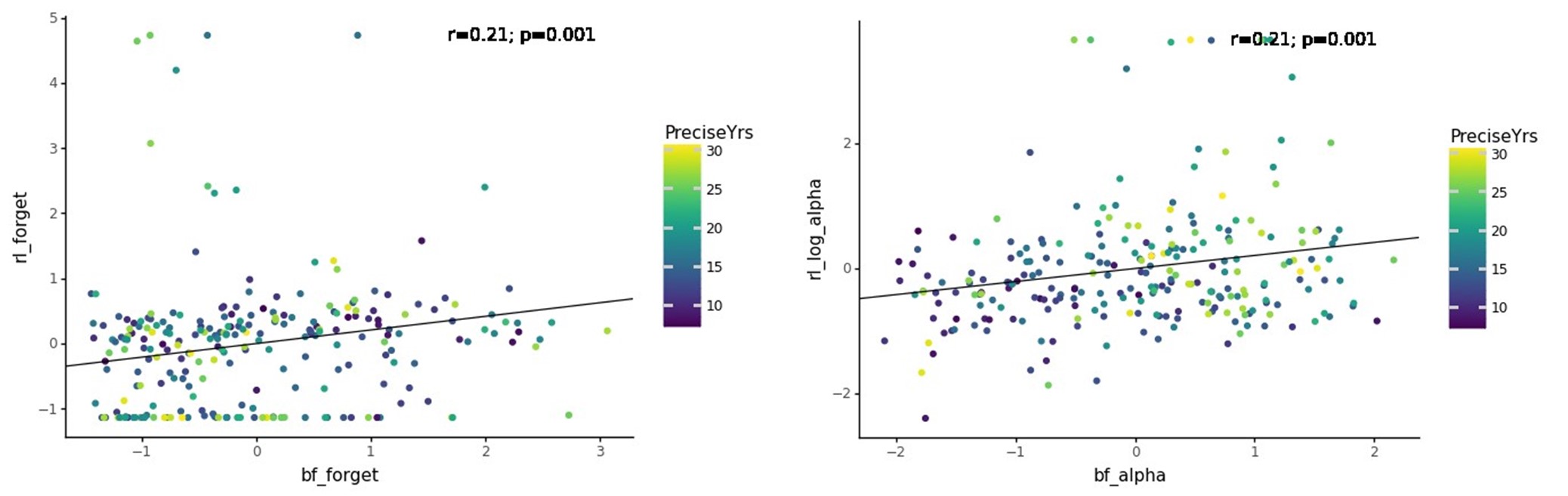
To answer the question in more detail, we have expanded our section about limitations stemming from parameter tradeoffs in the following way:
“One limitation of our results is that regression analyses might be contaminated by parameter cross-correlations (sections 2.1.2, 2.1.3, 2.1.4), which would reflect modeling limitations (non-orthogonal parameters), and not necessarily shared cognitive processes. For example, parameters alpha and beta are mathematically related in the regular RL modeling framework, and we observed significant within-task correlations between these parameters for two of our three tasks (suppl. Fig. H.10, H.11). This indicates that caution is required when interpreting correlation results. However, correlations were also present between tasks (suppl. Fig. H.9, H.11), suggesting that within-model trade-offs were not the only explanation for shared variance, and that shared cognitive processes likely also played a role.
Another issue might arise if such parameter cross-correlations differ between models, due to the differences in model parameterizations across tasks. For example, memory-related parameters (e.g., F, K in models A and C) might interact with learning- and choice-related parameters (e.g., alpha+, alpha-, noise/exploration), but such an interaction is missing in models that do not contain memory-related parameters (e.g., task B). If this indeed the case, i.e., parameters trade off with each other in different ways across tasks, then a lack of correlation between tasks might not reflect a lack of generalization, but just the differences in model parameterizations. Suppl. Fig. \ref{figure:S2AlphaBetaCorrelations} indeed shows significant, medium-sized, positive and negative correlations between several pairs of Forgetting, memory-related, learning-related, and exploration parameters (though with relatively small effect sizes; Spearman correlation: 0.17 < |r| < 0.22).
The existence of these correlations (and differences in correlations between tasks) suggest that memory parameters likely traded off with each other, as well as with other parameters, which potentially affected generalizability across tasks. However, some of the observed correlations might be due to shared causes, such as a common reliance on age, and the regression analyses in the main paper control for these additional sources of variance, and might provide a cleaner picture of how much variance is actually shared between parameters.
Furthermore, correlations between parameters within models are frequent in the existing literature, and do not prevent researchers from interpreting parameters---in this sense, the existence of similar correlations in our study allows us to address the question of generalizability and interpretability in similar circumstances as in the existing literature.”
- More generally, isn't relative generalizability the best we would expect given systematic variation in task context? I agree with the authors' point that the language used in the literature sometimes implies an assumption of absolute generalizability (e.g. same LR across any task). But parameter fits, interactions, and group differences are usually interpreted in light of a single task+model paradigm, precisely b/c tasks vary widely across critical features that will dictate whether different algorithms are optimal or not and whether cognitive functions such as WM or attention may compensate for ways in which humans are not optimal. Maybe a more constructive approach would be to decompose tasks along theoretically meaningful features of the underlying Markov Decision Process (which gives a generative model), and be precise about (1) which features we expect will engage additional cognitive mechanisms, and (2) how these mechanisms are reflected in model parameters.
We thank the reviewer for this comment, and will address both points in turn:
(1) We agree with the reviewer's sentiment about relative generalizability: If we all interpreted our models exclusively with respect to our specific task design, and never expected our results to generalize to other tasks or models, there would not be a problem. However, the current literature shows a different pattern: Literature reviews, meta-analyses, and discussion sections of empirical papers regularly compare specific findings between studies. We compare specific parameter values (e.g., empirical parameter priors), parameter trajectories over age, relationships between different parameters (e.g., balance between LR+ and LR-), associations between parameters and clinical symptoms, and between model variables and neural measures on a regular basis. The goal of this paper was really to see if and to what degree this practice is warranted. And the reviewer rightfully alerted us to the fact that our data imply that these assumptions might be valid in some cases, just not in others.
(2) With regard to providing task descriptions that relate to the MDP framework, we have included the following sentence in the discussion section:
“Our results show that discrepancies are expected even with a consistent methodological pipeline, and using up-to-date modeling techniques, because they are an expected consequence of variations in experimental tasks and computational models (together called "context"). Future research needs to investigate these context factors in more detail. For example, which task characteristics determine which parameters will generalize and which will not, and to what extent? Does context impact whether parameters capture overlapping versus distinct variance? A large-scale study could answer these questions by systematically covering the space of possible tasks, and reporting the relationships between parameter generalizability and distance between tasks. To determine the distance between tasks, the MDP framework might be especially useful because it decomposes tasks along theoretically meaningful features of the underlying Markov Decision Process.“
Another point that merits more attention is that the paper pretty clearly commits to each model as being the best possible model for its respective task. This is a necessary premise, as otherwise, it wouldn't be possible to say with certainty that individual parameters are well estimated. I would find the paper more convincing if the authors include additional information and analysis showing that this is actually the case.
We agree with the sentiment that all models should fit their respective task equally well. However, there is no good quantitative measure of model fit that is comparable across tasks and models - for example, because of the difference in difficulty between the tasks, the number of choices explained would not be a valid measure to compare how well the models are doing across tasks. To address this issue, we have added the new supplemental section (Appendix C) mentioned above that includes information about the set of models compared, and explains why we have reason to believe that all models fit (equally) well. We also created the new supplemental Figure D.7 shown above, which directly compares human and simulated model behavior in each task, and shows a close correspondence for all tasks. Because the quality of all our models was a major concern for us in this research, we also refer the reviewer and other readers to the three original publications that describe all our modeling efforts in much more detail, and hopefully convince the reviewer that our model fitting was performed according to high standards.
I am particularly interested to see whether some of the discrepancies in parameter fits can be explained by the fact that the model for Task A did not account for explicit WM processes, even though (1) Task A is similar to Task C (Task A can be seen as a single condition of Task C with 4 states and 2 possible visible actions, and stochastic rather than deterministic feedback) and (2) prior work has suggested a role for explicit memory of single episodes even in stateless bandit tasks such as Task B.
We appreciate this very thoughtful question, which raises several important issues. (1) As the reviewer said, the models for task A and task C are relatively different even though the underlying tasks are relatively similar (minus the differences the reviewer already mentioned, in terms of visibility of actions, number of actions, and feedback stochasticity). (2) We also agree that the model for task C did not include episodic memory processes even though episodic memory likely played a role in this task, and agree that neither the forgetting parameters in tasks A and C, nor the noise/exploration parameters in tasks A, B, and C are likely specific enough to capture all the memory / exploration processes participants exhibited in these tasks.
However, this problem is difficult to solve: We cannot fit an episodic-memory model to task B because the task lacks an episodic-memory manipulation (such as, e.g., in Bornstein et al., 2017), and we cannot fit a WM model to task A because it lacks the critical set-size manipulation enabling identification of the WM component (modifying set size allows the model to identify individual participants’ WM capacities, so the issue cannot be avoided in tasks with only one set size). Similarly, we cannot model more specific forgetting or exploration processes in our tasks because they were not designed to dissociate these processes. If we tried fitting more complex models that include these processes to these tasks, they would most likely lose in model comparison because the increased complexity would not lead to additional explained behavioral variance, given that the tasks do not elicit the relevant behavioral patterns. Because the models therefore do not specify all the cognitive processes that participants likely employ, the situation described by the reviewer arises, namely that different parameters sometimes capture the same cognitive processes across tasks and models, while the same parameters sometimes capture different processes.
And while the reviewer focussed largely on memory-related processes, the issue of course extends much further: Besides WM, episodic memory, and more specific aspects of forgetting and exploration, our models also did not take into account a range of other processes that participants likely engaged in when performing the tasks, including attention (selectivity, lapses), reasoning / inference, mental models (creation and use), prediction / planning, hypothesis testing, etc., etc. In full agreement with the reviewer’s sentiment, we recently argued that this situation is ubiquitous to computational modeling, and should be considered very carefully by all modelers because it can have a large impact on model interpretation (Eckstein et al., 2021).
If we assume that many more cognitive processes are likely engaged in each task than are modeled, and consider that every computational model includes just a small number of free parameters, parameters then necessarily reflect a multitude of cognitive processes. The situation is additionally exacerbated by the fact that more complex models become increasingly difficult to fit from a methodological perspective, and that current laboratory tasks are designed in a highly controlled and consequently relatively simplistic way that does not lend itself to simultaneously test a variety of cognitive processes.
The best way to deal with this situation, we think, is to recognize that in different contexts (e.g., different tasks, different computational models, different subject populations), the same parameters can capture different behaviors, and different parameters can capture the same behaviors, for the reasons the reviewer lays out. Recognizing this helps to avoid misinterpreting modeling results, for example by focusing our interpretation of model parameters to our specific task and model, rather than aiming to generalize across multiple tasks. We think that recognizing this fact also helps us understand the factors that determine whether parameters will capture the same or different processes across contexts and whether they will generalize. This is why we estimated here whether different parameters generalize to different degrees, which other factors affect generalizability, etc. Knowing the practical consequences of using the kinds of models we currently use will therefore hopefully provide a first step in resolving the issues the reviewer laid out.
It is interesting that one of the parameters that generalizes least is LR-. The authors make a compelling case that this is related to a "lose-stay" behavior that benefits participants in Task B but not in Task C, which makes sense given the probabilistic vs deterministic reward function. I wondered if we can rule out the alternative explanation that in Task C, LR- could reflect a different interpretation of instructions vis. a vis. what rewards indicate - do authors have an instruction check measure in either task that can be correlated with this "lose-stay" behavior and with LR-? And what does the "lose-stay" distribution look like, for Task C at least? I basically wonder if some of these inconsistencies can be explained by participants having diverging interpretations of the deterministic nature of the reward feedback in Task C. The order of tasks might matter here as well -- was task order the same across participants? It could be that due to the within-subject design, some participants may have persisted in global strategies that are optimal in Task B, but sub-optimal in Task C.
The PCA analysis adds an interesting angle and a novel, useful lens through which we can understand divergence in what parameters capture across different tasks. One observation is that loadings for PC2 and PC3 are strikingly consistent for Task C, so it looks more like these PCs encode a pairwise contrast (PC2 is C with B and PC2 is C with A), primarily reflecting variability in performance - e.g. participants who did poorly on Task C but well on Task B (PC2) or Task A (PC3). Is it possible to disentangle this interpretation from the one in the paper? It also is striking that in addition to performance, the PCs recover the difference in terms of LR- on Task B, which again supports the possibility that LR- divergence might be due to how participants handle probabilistic vs. deterministic feedback.
We appreciate this positive evaluation of our PCA and are glad that it could provide a useful lens for understanding parameters. We also agree to the reviewer's observation that PC2 and PC3 reflect task contrasts (PC2: task B vs task C; PC3: task A vs task C), and phrase it in the following way in the paper:
“PC2 contrasted task B to task C (loadings were positive / negative / near-zero for corresponding features of tasks B / C / A; Fig. 3B). PC3 contrasted task A to both B and C (loadings were positive / negative for corresponding features on task A / tasks B and C; Fig. 3C).”
Hence, the only difference between our interpretation and the reviewer’s seems to be whether PC3 contrasts task C to task B as well as task A, or just to task A. Our interpretation is supported by the fact that loadings for tasks A and C are quite similar on PC3; however, both interpretations seem appropriate.
We also appreciate the reviewer's positive evaluation of the fact that the PCA reproduces the differences in LR-, and its relationship to probabilistic/deterministic feedback. The following section reiterates this idea:
“alpha- loaded positively in task C, but negatively in task B, suggesting that performance increased when participants integrated negative feedback faster in task C, but performance decreased when they did the same in task B. As mentioned before, contradictory patterns of alpha- were likely related to task demands: The fact that negative feedback was diagnostic in task C likely favored fast integration of negative feedback, while the fact that negative feedback was not diagnostic in task B likely favored slower integration (Fig. 1E). This interpretation is supported by behavioral findings: "Lose-stay" behavior (repeating choices that produce negative feedback) showed the same contrasting pattern as alpha- on PC1. It loaded positively in task B, showing Lose-stay behavior benefited performance, but it loaded negatively on task C, showing that it hurt performance (Fig. 3A). This supports the claim that lower alpha- was beneficial in task B, while higher alpha- was beneficial in task C, in accordance with participant behavior and developmental differences.“
Author Response:
Reviewer #1 (Public Review):
The authors make juxtacellular recordings on awake mice, which should yield clear responses of actions potentials, and employ a number of manipulations to silence pathways. They also record from a "non"-whisker secondary thalamic region, LP, as a null hypothesis to establish if certain effects are related to "behavior" - read arousal or saliency". I have no major qualms.
In light of Petersen's paper (Cell Reports 2014) on cholinergic effects on spike rates in primary whisker somatosensory cortex, I can imagine that the authors considered measuring from cholinergic neurons in nucleus basalis during whisking. I'll assume that this is easier said than done. As such, the current manuscript passes my threshold for publication modulo issues raised below that are related to anatomy.
The cholinergic experiments are an interesting idea. However, inactivation of S1 did not change the relationship between POm and whisking, suggesting that cholinergic modulation of S1 and thereby corticothalamic output are not the key mechanism. It is conceivable that acetylcholine modulates POm directly, but the critical experiments would involve extensive manipulations of POm (a whole additional study). Nevertheless, we have added a reference to Eggermann & Petersen and discussed this issue further in the revision.
I provide a figure-by-figure critique:
(1) Recent work from Deschênes et al (Neuron 2016) points to a description of whisking in terms of Angle = Set-point_angle - Whisking-amplitude [1 + cosine(Phase - Phase_0)], where Phase is a rapidly varying, typically rhythmic function of time. Why not use this notation as opposed to yet another descriptive statistic and report the kinetics as the time averaged parameters , i.e., the most forward position, and ,Whisking-amplitude>, i.e., the half-amplitude of the average whisk?
We are not entirely sure what the reviewer means by “another descriptive statistic” as we do not introduce new approaches for analyzing whisking in this paper. (Perhaps the reviewer refers to “median angle”, which is an average of all the whisker positions on a single frame. We use this measurement because our videos contain the entire whisker field rather than just a single whisker as in our other studies, e.g. Hong et al 2018, Rodgers et al 2021). We based our parameterization of median angle on two publications: Hill et al (2011 Neuron) and Moore et al (2015 PLoS Biology). Moore et al describes whisking as a function of phase, amplitude, and midpoint:
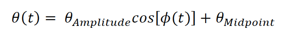
where 𝜃(t) is the median whisker angle at time 𝑡 , 𝜙 is the phase as computed by the Hilbert transform of the filtered whisker angle, 𝜃^Amplitude is the difference between the most protracted and retracted whisker positions over a single cycle, and 𝜃^midpoint is the central angle of a single whisk cycle. As we understand the reviewer, we are using the formulation they describe. We are happy to consider alternate formulations if we are missing something.
A critical issue is to confirm where the recording were made. This the authors should supply at least a typical record of anatomy from their POm as well as VPM and LP recording. The beauty of the juxtacellular technique is that neurons can be labeling after the recording
We used the juxtacellular recording technique for its superior recording quality. We did not label individual cells after recording because we recorded multiple cells per animal over several days. The number of cells would complicate matching of filled cells to recorded physiological data, and biotin filling is not stable over multiple days (beyond 36 hours). Instead, as described in the original manuscript, we tracked the relative locations of all inserted pipettes and labeled the final track with DiI. Cells were roughly localized along the tracks using relative microdrive depths. Due to the morphological homogeneity of thalamic neurons, filling individual cells would not be more informative than labelling the recording site with DiI. New Figure 1 – figure supplement 1 includes representative histology images from our recordings in POm, VPM, LP, and M1.
(2) Did the authors make sure that the mystacial pad is not moving by imaging the pad as opposed to just the shaft of the whiskers? The top view in Figure 1A makes this hard to check.
To address this concern, we provide new data, in which both the cut and uncut sides of the face of mice were imaged. We measured the movement of the mystacial pads as motion energy – the mean absolute difference in pixel values across video frames. The motor nerve surgery almost completely abolished movement of the mystacial pad. A new figure panel (Figure 2B) demonstrates the movement of the normal and paralyzed mystacial pads.
Further, did the authors perform post-hoc anatomy to insure that both the ramus buccolabialis inferior and ramus buccolabialis superior muscles were cut? This is critical; it is also easy to leave the maxillolabialis (external retractor) innervated if the cut is too far rostral.
We did not attempt to cut muscles. We only cut the motor nerve. We did not examine the face post mortem, as it was obvious that both whisker and mystacial pad movement were absent (as in new Figure 2B).
(3/4) As relevant background, the text should note that whisker primary motor cortex maintains a copy of the envelope of the whisking, i.e., an ill-defined summation of set-point and amplitudes, even if the sensory input (Ahrens & Kleinfeld J Neurophysiol 2004) or motor output (Fee et al. J Neurophysiol 1997) in the periphery are cut.
The Results text now cites these papers as motivation for the experiments of Figure 3.
(6/7) Same comments in (1) in whisking parameters and anatomy.
As we discussed in (1), we are using the conventional parameterization of others. Histological examples are now included in Figure 1 – figure supplement 1.
Reviewer #3 (Public Review):
Previous studies in urethane-anesthetized rats (PMID 16605304) proposed that POm cells code whisker movements. This was observed using "artificial whisking" procedures (stimulating the motor nerve to produce a whisking-like movement). It has been clear for some time now that there are substantial (obvious) differences between this procedure and natural whisking. In addition, under urethane-anesthesia animals are in a sleep-like state that is very dissimilar to waking (although some work has tested the effect of network state on artificial whisking responses in both primary thalamus and cortex; see 25505118). In the present study, the authors measured activity in POm cells during whisking in awake (head-fixed) mice to determine if they code whisking movement. However, this seems to have already been done previously. For instance, Moore et al (2015; 26393890) found that coding of whisking in the ascending paralemniscal pathway, including POm, is "relatively poor" (as stated in the abstract), which is the same conclusion reached in the present study. The authors should clarify the main differences observed in whisking coding between their study and previous work.
The authors then focused on the idea that POm codes behavioral state. However, many studies have previously determined that state has a great impact on thalamocortical dynamics; thalamic cells are very sensitive to state including cells in primary whisker thalamic nuclei, such as VPM, and these effects can be produced by neuromodulators (see work by Castro-Alamancos' group, for example, 16306412). There is nothing special about VPM in this regard; other thalamic sensory nuclei are also sensitive to behavioral state and neuromodulators. Therefore, the observation that POm and LP cells are sensitive to state is unsurprising. It is also known that these thalamic state changes have a great impact on the state of the cortex (see 20053845), which seems very relevant to the main conclusion. The POm has to be doing something different than coding behavioral state since most thalamic nuclei do this. The study did not identify the role of POm, which certainly has to be different from LP (otherwise, why would these nuclei be differentiated?). POm is unlikely to be specialized for monitoring state since this is done by most of the thalamus -including VPM, which projects to the same cortical region. Thus, while it is interesting that most of the whisker-related activity in POm is state-dependent, the study does not clarify the role of POm.
We have added the references we did not already include to our text and improved our discussion.
Prior studies (such as Moore et al 2015 and Urbain et al 2015) have previously characterized the encoding of whisker motion in POm. Indeed, we note the consistency between our results and such studies in both the introduction and conclusion. Here we expand upon prior studies to directly test two prominent hypotheses about the role of the paralemniscal pathway: that it encodes sensory reafference, and that it inherits a motor efference copy from cortical and subcortical regions. We present the impact of several manipulations of the vibrissal system (facial paralysis, cortical silencing, and lesion of superior colliculus) on thalamic activity that, to our knowledge, have not been previously reported. Moreover, we leveraged a novel comparison of POm and LP to test whether movement‐correlations of POm reflected true motor modulation or rather state dependency. We have provided evidence that the coupling of POm activity to whisking reflects state rather than motor signals. We never suggested that POm is a unique monitor of behavioral state. We suggest instead that secondary thalamic nuclei may be state‐modulated and have specific impacts on response gain and plasticity in their respective cortical areas. While our work is consistent with previous studies, we believe these results are novel extensions of past work.
The main strength of the study is that it was performed in awake mice with behavioral state monitoring, which contributes to the current understanding of active whisking coding in the complex network of the vibrissa system.
In our opinion, the main strength of our study is its multiple manipulations to test the sources of modulation and the leveraging of a POm‐LP comparison. We have revised the text to reinforce these points.
Author Response
Reviewer #3 (Public Review):
Q1) The manuscript reports that in vitro fertilization (including in vitro culture) of mouse embryos seemingly originates metabolic alterations probably caused by enhanced oxidative stress compared to in vivo development. Such alterations apparently increase anaerobic glycolysis, as evidenced by altered pH and lactate levels, and remain after birth, as evidenced by altered protein abundance of MCT1 and LDHB.
The manuscript concludes that IVF alters embryo metabolism, increasing oxidative damage and glycolytic activity. The topic is interesting but I consider that the conclusions are not well supported by the experiments:
1) In vivo generated blastocysts are analyzed at a more advanced developmental stage than their in vitro counterparts as evidenced by their increased cell number (70 vs. 50 cells). In this regard, the developmental timing when in vitro generated blastocysts are collected is undisclosed in the Materials and methods. This has an obvious effect on all experiments as the differences observed may be stage-specific rather than IVF vs. in vivo.
A1) Thank you for the comment. The reviewer is correct and it is indeed well known that in vitro fertilization and embryo culture results in profound changes to the embryo. Overall, embryos generated in vitro are delayed compared to embryos generated in vivo. To control for this, as done in our past publications (Belli 2019; Bloise 2014; Delle Piane 2010; Giritharan 2012; Giritharan 2010; Giritharan 2006; Giritharan 2007; Rinaudo 2006; Rinaudo 2004), or by others (Doherty 2000; Ecker 2004; Weinerman 2016), we limited the analysis to expanded blastocysts of similar morphology (under microscopic examination) in all of the groups. Therefore the embryos appeared morphological similar in all of the groups. As an alternative, we could have waited longer time in vitro, but this would have resulted in embryo hatching and being not morphological similar to in vivo embryos. In addition, the 2 IVF groups provide an internal control: embryos were at the same developmental stage, but showed significant changes in metabolism and cell numbers. (96 hours of culture +13-14hours for egg collection+ 4hours of fertilization= time post HCG administration)
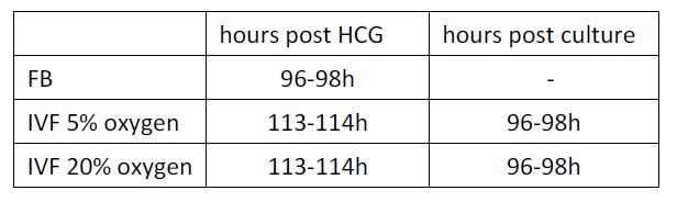
We have added this information as follows: Line 377-382: To control for the known delay in development after culture in vitro, for all experiments, only expanded blastocysts of similar morphology were used, as done before (Doherty 2000; Rinaudo 2006; Rinaudo 2004). The in vivo-generated blastocysts were isolated by flushing 96-98 hours after hCG administration. IVF- 5% O2 and 20% O2 generated embryos reached the blastocyst stage after 96-98 hours following in vitro culture and 113-114 hours after hCG administration, respectively.
Q2) Several methods are not reliable to quantify the parameters analyzed. For instance, determining protein content by immunofluorescence has been largely shown to be misleading as immunofluorescence can be affected by multiple parameters. Intracellular pH was also analyzed by an assay also based on immunofluorescence, which can also be affected by embryo size (the blastocoel is a call-devoid cavity). These analyses are not reliable.
A2) Thank you for the comments.
We appreciate the comments and concerns. Any single method can result in error and possible bias. Immunofluorescence analysis is a robust method that has been used to analyze the distribution of proteins in cells or tissues. For instance, oxidative stress (Liu et al., 2022, Reprod Domest Anim), several signaling molecule (Spirkova et al., 2022, Biol Reprod) and DNA methylation level (Diaz et al, 2021, Fron Gent) have been measured by immunofluorescence in preimplantation embryos and oocytes. It our study, to minimize errors, we followed exactly the same protocol and we found immunofluorescence to be reliable. In addition, global proteomics analysis of blastocysts provide partial independent confirmation of our results. While LDH-A and MCT1 were not detected, LDH-B was detected and found to be lower in IVF blastocysts, exactly as show by IF studies. Finally, western blot analysis of adult tissues confirmed reduction in LDH-B and MCT-1 levels.
These comments have been added to the discussion as follows:
Line 299-302: Unsupervised global proteomics analysis revealed that LDH-B was downregulated in IVF embryos. We confirmed these results by performing immunofluorescence studies. In addition we found that IVF embryos showed downregulation of both LDHA and B and of the monocarboxylate transporter, MCT 1, providing an explanation for the increase in their lactate levels
Regarding pH measurement: to control for the possible variation in blastocoel size in different embryos, we compared immunofluorescence level of only the inner cell mass and trophoblast region of blastocysts and excluded the blastocoel region.
This clarification has been added to the method section as follow:
Line 488-491: To control for the possible variation in blastocoel size in different embryos, we compared immunofluorescence level of only the inner cell mass and trophoblast region of blastocysts and excluded the blastocoel region.
Q3) Identifying proteins and metabolites in such small samples is technically difficult and error-prone, requiring validation by alternative techniques.
We appreciate the comments and concerns. Any single method can result in error and possible bias. Immunofluorescence analysis is a robust method that has been used to analyze the distribution of proteins in cells or tissues. For instance, oxidative stress (Liu 2022), several signaling molecule (Spirkova 2022) and DNA methylation level (Diaz 2021) have been measured by immunofluorescence in preimplantation embryos and oocytes. It our study, to minimize errors, we followed exactly the same protocol and we found immunofluorescence to be reliable. In addition, global proteomics analysis of blastocysts (triplicate for each group; n=100 blastocysts for each replicate; total 900 embryos). provide partial independent confirmation of our results. While LDH-A and MCT1 were not detected, LDH-B was detected and found to be lower in IVF blastocysts, exactly as show by IF studies. Finally, western blot analysis of adult tissues confirmed reduction in LDH-B and MCT-1 levels.
These comments have been added to the discussion as follows:
Line 299-302: Unsupervised global proteomics analysis revealed that LDH-B was downregulated in IVF embryos. We confirmed these results by performing immunofluorescence studies. In addition we found that IVF embryos showed downregulation of both LDHA and B and of the monocarboxylate transporter, MCT 1, providing an explanation for the increase in their lactate levels
Q4) Given the small size of these embryos (~80 µm diameter), it is unclear how they can alter significantly the composition of 500 µl of medium (106 their own volume).
To collect 300 blastocysts, we performed multiple IVF, each IVF resulting in 10-20 blastocysts cultured in 30 microliters of media. While intracellular lactate and pyruvate were performed on the embryos collected, the media from different experiments was pooled to a final 500 microliter volume. Lactate and pyruvate levels were measured in this final volume for each group of embryo (FB, IVF5% and IVF20%)
This has been clarified in the method section as follows:
Line 516-519: To collect 300 blastocysts, we performed multiple IVF, each IVF resulting in 10-20 blastocysts cultured in 30 microliters of media. While intracellular lactate and pyruvate were performed on the embryos collected, the media from different experiments was pooled to a final 500 microliter volume.
Q5) The metabolic changes observed in the offspring lack a mechanistic explanation.
Thank you for the comment. We can formulate a hypothesis in which (Figure 8) oxidative stress from in vitro condition increase ROS and induce oxidative damage resulting in a shift toward Warburg metabolism, given that lactate is a critical energy source (Brooks, 2018). The higher intracellular lactate levels will likely induce epigenetic changes, to favor Warburg metabolism during development, as an embryonic attempt to optimize growth based on the environment predicted to be experienced in the future. When the environment does not match the prediction, disease risk increases (Godfrey 2007). Low lactate would be beneficial in a setting of low food resources because it could favor lipolysis (Brooks, 2020). In fact, lactate activates the hydroxycarboxylic acid receptor 1 (HCAR1), a G protein-coupled receptor, which in turn inhibits lipolysis in fat cells via cAMP and CREB (Liu 2009). However, since there is an abundance of food in our society, this mismatch could predispose IVF concepti to develop chronic disease like glucose intolerance.
This hypothesis has been added to line 333-344:
In summary, we can formulate a hypothesis in which (Figure 8) oxidative stress from in vitro condition increase ROS and induce oxidative damage resulting in a shift toward Warburg metabolism, given that lactate is a critical energy source (Brooks, 2018). The higher intracellular lactate levels will likely induce epigenetic changes, to favor Warburg metabolism during development, as an embryonic attempt to optimize growth based on the environment predicted to be experienced in the future. When the environment does not match the prediction, disease risk increases (Godfrey 2007). Low lactate would be beneficial in a setting of low food resources because it could favor lipolysis (Brooks, 2020). In fact, lactate activates the hydroxycarboxylic acid receptor 1 (HCAR1), a G protein-coupled receptor in turn inhibits lipolysis in fat cells via cAMP and CREB (Liu 2009). However, since there is an abundance of food in our society, this mismatch could predispose IVF concepti to develop chronic disease like glucose intolerance.
Author Response
Public Evaluation Summary
The authors aim to tackle a fundamental question with their study: whether there is a direct age-associated increase of transcriptional noise. To investigate this question, they develop tools to analyze single-cell sequencing data from mouse and human aging datasets. Ultimately, application of their novel tool (Scallop) suggests that transcriptional noise does not change with age, changes in transcriptional noise can be attributed to other sources such as subtle shifts in cell identity. This study is in principle of broad interest, but it currently lacks a definitive demonstration of the robustness of Scallop. Systematic testing of this new package would ultimately strengthen the key conclusion of the work and give additional users more confidence when using the tool to estimate expression noise.
We have now attempted to further demonstrate the robustness of Scallop by performing a more systematic analysis and a side-by-side comparison to other existing methods using a set of artificially generated datasets. These analyses have resulted in the inclusion of six supplementary figures that are presented in the subsections Scallop membership score accurately identifies transcriptionally noisy cells, Ability to detect noisy cells within cell types, Effect of cellular composition, Effect of dataset size, Effect of feature expression and Effect of cell type marker expression within the Results section of the revised manuscript.
We have also included a supplementary figure showing an in-depth analysis of a dataset where ageassociated increase in transcriptional noise was detected using alternative methods, but whose closer dissection has revealed that the difference in noise is due to a single donor and to the choice of methods. We discuss this is in the subsection Distance-to-centroid methods detect transcriptionally stable cell subtypes as transcriptional noise within the Results section.
Finally, we have revised the manuscript to clarify the main points raised by the reviewers: the definition of transcriptional noise, the reasoning behind the choice of the single-cell aging datasets and Leiden’s rationale. Also, we have expanded the description of the method to make the definition of membership score more clear to the readers, and discussed the implications of our main findings (a lack of evidence for age-related transcriptional noise) in the broader context of theories of aging.
Reviewer #1 (Public Review):
In the present study, Ibanez-Sole et al evaluate transcriptional noise across aging and tissues in several publicly available mouse and human datasets. Initially, the authors compare 4 generalized approaches to quantify transcriptional noise across cell types and later implement a new approach which uses iterative clustering to assess cellular noise. Based on implementation of this approach (scallop), the authors survey noise across seven sc-seq datasets relevant for aging. Here, the authors conclude that enhanced transcriptional noise is not a hallmark of aging, rather changes in cell identity and abundances, namely immune and endothelial cells. The development of new tools to quantify transcriptional noise from sc-seq data presents appeal, as these datasets are increasing exponentially. Further, the conclusion that increased transcriptional noise is not a defined aspect of aging is clearly an important contribution; however, given the provocative nature of this claim, more comprehensive and systematic analyses should be performed. In particular, the robustness and appeal of scallop is still not sufficiently demonstrated and given the complexity (multiple tissues, species and diverse relative age ranges) of datasets analyzed, a more thorough comparison should be performed. I list a few thoughts below:
Initially, the authors develop Decibel, which centralizes noise quantification methods. The authors provide schematics shown in Fig 1, and compare noise estimates with aging in Fig 2 - Supplement 2. Since the authors emphasize the necessary use of scallop as a ”better” pipeline, more systematic comparisons to the other methods should be made side-by-side.
We thank the reviewer for their positive assessment of the manuscript and their suggestions. We agree that side-by-side benchmarking of Scallop with the methods implemented in Decibel, as well as a more thorough analysis on the effect of different features such as dataset size, cellular composition, etc. might have on the output of Scallop will reinforce the main points of the manuscript. To experimentally respond to these requests, we took advantage of a set of four artificial datasets previously generated by us with the R package splatter (v1.10.1; as described in Ascensión et al. [1]). In the present work, we first run a side-by-side comparison between Scallop and two distance-to-centroid (DTC) methods on the four artificial datasets with increasing degrees of transcriptional noise present in them (the novel data are included as Figure 1 – Figure supplement 1 in the revised manuscript). Then, we compared Scallop to one DTC method regarding their ability to detect noisy cells in different cell types (Figure 1 – Figure supplement 2). Finally, we implemented four simulations to test the effect of the following features on the performance of Scallop: cellular composition (Figure 1 – Figure supplement 3), dataset size (Figure 1 – Figure supplement 4), number of genes (Figure 1 – Figure supplement 5) and marker gene expression (Figure 1 – Figure supplement 6). A summary of these results follows.
Side-by-side comparison of Scallop vs DTC methods
Each of the four artificial datasets used consists of 10K cells, from 9 populations, named Group1 to Group9, with the following relative abundances: 25, 20, 15, 10, 10, 7, 5.5, 4, and 3.5%, respectively. The four datasets only differ in the de.prob parameter used in their generation. The de.prob parameter determines the probability that a gene is differentially expressed between subpopulations within the dataset. The greater the de.prob value, the more differentially expressed genes there will be between clusters, meaning that the different cell types present in the dataset will cluster in a more robust way. Decreasing the value of de.prob results in datasets with noisy cells, with populations that do not have such a strong transcriptional signature. In order to study how Scallop can capture the degree of robustness with which cells of the same cell type cluster together, we selected four de.prob values (0.05, 0.016, 0.01 and 0.005) and measured transcriptional noise using Scallop and two DTC methods, the whole transcriptome-based Euclidean distance to cell type mean and the invariant gene-based Euclidean distance to tissue mean expression. These two methods were selected because GCL does not yield a transcriptional noise measure per cell, so no comparisons can be made with respect to the amount of noisy cells the method is able to detect within a cluster. Similarly, comparing Scallop to the ERCC spike in-based method was not possible for artificial datasets. Importantly, these analyses showed that Scallop, unlike DTC methods, was able to discern between the core transcriptionally stable cells within each cell type cluster from the more noisy cells that lie in between clusters (provided in the Figure 1 - Supplement 1 of revised manuscript).
Effect of dataset features on the performance of Scallop
We simulated five artificial datasets with the same nine cell type populations but whose relative abundances were different between datasets. We used the imbalance degree (ID) to measure class imbalance in each of them and to make sure that the selected cell compositions represented a wide range of imbalance degrees (to this end, we explored ID values between 1.2 and 5.3). The ID provides a normalized summary of the extent of class imbalance in a dataset in so-called ”multiclass” settings, that is to say, where more than two classes are present. It was specifically developed to improve the commonly used imbalance ratio (IR) measurement, whose calculation only considers the abundance of the most and the least popular classes and which gives the same summary for datasets with different numbers of minority classes. The presence of multiple minority classes is not uncommon in single-cell RNAseq datasets, as tissues might contain several rare cell types. We observed that the transcriptional noise measurements provided by Scallop were very robust to changes in imbalance degree (see Figure 1 - Supplement 3), both in qualitative and in quantitative terms. For instance, Group2 and Group8 were always detected as the most stable and noisiest cell types, respectively, regardless of their relative abundance in the dataset, and their average percentage of noise had little variation between different ID values: it ranged between 0-0.14% (Group2) and 16-18% (Group8).
The effect of dataset size (number of cells) and the number of genes was evaluated by generating versions of an artificial dataset where cells/genes had been subsampled from an original artificial dataset (the one generated with de.prob=0.001). We tested datasets sized 1,000-10,000 cells and with a number of genes between 5,000 and 14,000. Dataset size had nearly no impact on the transcriptional noise measurements provided by Scallop (Figure 1 - Supplement 4 of the revised manuscript). The average percentage of transcriptional noise per cell type remained within a narrow range as we implemented a ten-fold increase in dataset size. Perhaps more strikingly, removing the expression of most genes did not substantially impact transcriptional noise measurements per cell type (Figure 1 - Supplement 5). The variation when removing half of the genes (7,000 genes) was minimal, and we did not see important changes in transcriptional noise measurements unless over 60% of the genes from the original dataset were removed. For example, Figure 1 - Supplement 5C shows that noise measurements suffer important variations when removing 8,000 and 9,000 genes (and therefore keeping 6,000 and 5,000 genes, respectively), but only some cell types (Groups 4, 7, 8 and 9) were affected by these variations.
In order to measure the effect marker gene expression has on the membership with which cells are assigned to their cell type cluster, we ran a simulation where the top 10 markers for a cell type were removed from the dataset one by one, so that the first simulation lacked the expression of the Top1 marker, the second simulation had the effect of the first 2 markers removed (Top1 and Top2), and so on. Then, we ran Scallop on each of the resulting datasets and observed a steady increase in transcriptional noise associated with that cell type. This provided evidence that the strength of cell type marker expression in a cluster is directly related to its transcriptional stability (or lack of transcriptional noise). We included the result of this experiment in the revised version of the manuscript (Figure 1 - Supplement 6).
In conclusion, by using artificially generated datasets where the ground truth (cell type labels, degree of noise, etc) was known, the newly provided systematic analyses showed that Scallop had a remarkably robust response to said changes in dataset features, further reinforcing the manuscript conclusions.
For example, scallop noise estimates (Fig 2) compared to other euclidean distance-based measures (Fig 2 supplement 2) looks fairly similar.
It is true that some datasets show similar trends regardless of the transcriptional noise quantification method. For instance, the murine brain dataset by Ximerakis et al. shows no overall change in noise between the age groups across different methods. However, we do observe important differences in other examples. This is the case of the human pancreas dataset by Enge et al. and the human skin dataset by Solé-Boldo et al., where not only the magnitude but also the directionality of the trend are different depending on the method used to measure noise. In the former, three methods (Scallop, invariant gene-based Euclidean distance to average tissue expression and GCL) show an age-related increase in noise, whereas one method (whole transcriptome-based Euclidean distance to the cell type mean) shows a decrease in noise. In the latter, two methods (Scallop and GCL) yield a decrease in noise and the two DTC methods measure a mild increase in noise. These inconsistencies can now be reconciled with our proposed explanation that said ”noise” may actually be referring to substantially different biology in the diverse experimental settings.
Are downstream observations (ex lung immune composition changes more than noise) supported from these methods as well? If so, this would strengthen the overall conclusion on noise with age, but if not, it would be relevant to understand why.
Studying changes in cell type composition in the lung and other aged tissues would be highly pertinent. Nevertheless, we have measured changes in cell type composition using only one method that is based on Generalized Linear Models, covered in the subsection Age-related cell type enrichment of the Methods. The methods that we have compared in our study (DTC methods, ERCC-based methods, GCL, etc.) were all designed to measure transcriptional noise, but not changes in cell type composition.
Whether the effects of cell type composition changes are bigger than changes in noise for the rest of the methods used to measure noise was probably not clear enough in the original manuscript. We found no evidence for an increase in noise associated with aging, regardless of the method used. Although not included in the manuscript, we did generate heatmaps similar to the one shown in Figure 3B for each of the noise quantification methods. However, as the heatmap on the right side (the one showing cell type enrichment) was identical in each figure, we considered them to be redundant and decided not to include them, since they did not provide any additional insight besides giving more examples of lack of evidence for transcriptional noise, this time at the cell type level. We consider that the lack of evidence was already well demonstrated in the previous analyses (Figure 2 and Figure 2 - Supplement 2.
Similarly, the ’validation of scallop seems mostly based on the ability to localize noisy vs stable cells in Fig 1 supplement 1 and relative robustness within dataset to input parameters (Fig 1 supplement 2). A more systematic analysis should be performed to robustly establish this method. For example, noise cell clustering comparisons across the 7 datasets used. In addition, the Levy et all 2020 implemented a pathway-based approach to validate. Specifically, surrogate genes were derived from GCL value where KEGG preservation was used as an output. Similar additional types of analyses should be performed in scallop.
We believe that this legitimate concern is now solved with the newly included data. In particular, with the systematic comparison between Scallop and DTC methods on three artificially generated datasets with different degrees of transcriptional noise provided in Figure 1 - Supplement 2. The ability of Scallop to detect cells that are particularly noisy within a cell type, or cells that lie between cell types, may represent its biggest advantage with respect to other methods. DTC methods fail to discern between stable and noisy cells within cell types. Also, in our analysis, DTC methods were unable to distinguish between cell types that have a marked transcriptional program (which systematically cluster together) and those that have a less clear transcriptomic identity (which have at least part of their cells be assigned to other cell types across bootstrap iterations). However, comparing the performance of Scallop on the same datasets showed that our method was able distinguish between the two cases.
The conclusion that immune and endothelial cell transcriptional shifts associate more with age than noise are quite compelling, but seem entirely restricted to the mouse and human lung datasets. It would be interesting to know if pan-tissues these same cell types enrich age-related effects or whether this phenomenon is localized.
We agree with the reviewer that it would be very interesting to see whether a change in cell type composition (and particularly, an increase in abundance of immune cell types) is observed in aged tissues other than the lung. Qualitative cell type composition changes in the aging lung have been described in the literature [5]. Specifically, the higher abundance of immune cell types was observed in a single-nucleus RNAseq dataset of cardiopulmonary cells in Macaca fascicularis [6]. However, we believe that trying to answer the question whether this phenomenon holds in other tissues would require a systematic analysis of several datasets for each tissue with a sufficient number of donors/individuals in each of them. This is because our approach to measure age-associated cell type enrichment using generalized linear models relies heavily on having multiple biological replicates for each age group. Unfortunately, this is not the case for most published single-cell RNAseq datasets of aging. In any case, we have toned down the last sentence in the subsection Changes in the abundance of the immune and endothelial cell repertoires characterize the human aging lung by making it more clear that our claim regarding changes in the cellular composition of aged tissues is based on lung datasets (the text in italics represents what was added in the revised version of the manuscript):
"Even though the evidence for changes in tissue composition are based on a single tissue, we hypothesize that these facts may have influenced previous analyses of transcriptional noise associated with aging."
As discussed in the original manuscript, there is evidence published by other groups pointing out to pantissue changes in cellular composition with age, which undoubtedly will influence those analyses that did not pay attention to cellular composition changes in the datasets that they compared. Cellular composition is in fact a very important aspect that has been greatly overlooked. In fact, only one [7] out of the seven articles that had measured transcriptional noise in aging (the datasets used in Figure 2) had attempted to remove its effect by subsampling cells to balance compositions between age groups prior to their noise analysis. In any case, we do not believe this is the only phenomenon underlying the purported increase in transcriptional noise associated with age. Each dataset will most probably have different issues that the authors originally misread as an increase in noise or loss of cellular identity of a particular organ or tissue. As an additional example of such phenomena, we have now included a re-analysis of the data by Enge et al. [3] on ”noisy” β-cells in the aged human pancreas (Figure 5–Figure supplement 2 of the revised manuscript). In this case, rather than observing an age-dependent pattern, the 21-year-old donor presents much lower transcriptional noise values than the rest of the donors. However, there is no significant difference between the 22-year-old donor and the rest of the donors. We conclude that the statistically significant differences between the ”young” and ”old” age categories can be attributed to the abnormal noise values obtained for the 21-year-old donor, of uncertain origin. Finding out all causes of apparent transcriptional noise in other organs and tissues would be too lengthy, and certainly out of scope for the present manuscript.
Related to these, there does not seem to be a specific rationale for why these datasets (the seven used in total or the lung for deep-dive), were selected. Clearly, many mouse and human sc-RNA-seq datasets exist with large variations in age so expanding the datasets analyzed and/or providing sufficient rationale as to why these ones are appearing for noise analyses would be helpful. For example, querying ”aging” across sc-seq datasets in Single cell portal yields 79 available datasets: https://singlecell.broadinstitute. org/single_cell?type=study&page=1&terms=aging&facets=organism_age%3A0%7C103%7Cyears.
We now realize that the reasoning behind our selection of aging datasets was not sufficiently clear in the original manuscript. We thank the reviewer for pointing out this omission. We have made a more explicit reference to Appendices 2, 3, 4 and 6 in the revised manuscript. The seven selected scRNAseq datasets are those where transcriptional noise had originally been measured by the authors, using the computational methods that we later implemented in Decibel. Our aim was to first recapitulate previous reports of transcriptional noise using our novel method (Scallop). Thus, we downloaded all publicly available scRNAseq datasets of aged tissues where transcriptional noise had explicitly been measured. Some of them had reported an increase in transcriptional noise only in some cell types (for instance, the human aged pancreas dataset by Enge et al. [3]), whereas others found an increase in most cell types [7]. Appendix 2 summarizes the main features of those seven datasets (tissue, organism and number of cells) and provides information on whether an increase in transcriptional noise was observed in the original article where they were published. Additionally, the ”scope” column indicates where that increase was found (in which cell types), and the ”Method” column briefly describes the computational method used to measure transcriptional noise in that article. Appendix 3 provides information on the final datasets that were used in our analysis (Figure 2). Not every sample from the original dataset was included, so the inclusion criteria are specified there, as well as the number of cells, individuals and age of each of the cohorts. Appendix 4 shows the abnormal count distribution of two samples that were discarded from the Kimmel lung dataset. As for the selection of lung for the deep dive, the reason was that this was the organ with most datasets available, both for mouse and human. Appendix 6 provides information on the number of cells and donors per age cohort in the human lung datasets included in this study.
We have included the following sentence in the Increased transcriptional noise is not a universal hallmark of aging subsection in the Results:
"We provide a summary of the main characteristics of each dataset, as well as the findings regarding transcriptional noise obtained in each of the original studies, whether changes in transcriptional noise were restricted to particular cell types, and the computational method used to measure noise (see Appendix 2)."
The analysis that noise is indistinguishable from cell fate shifts is compelling, but again relies on one specific example where alternative surfactant genes are used as markers. The same question arises if this observation holds up to other cell types within other organs. For example the human cell atlas contains over dozens of tissue with large variations in age (https://www.science.org/doi/10.1126/science. abl4290).
We sympathize with this comment but hope that the reviewer will agree with us that providing an additional example of different phenomena originally reported as ”transcriptional noise” (in this case in aged human pancreas; see Figure 5 – Figure supplement 2), but actually reflecting something else, may be sufficient to prevent interested readers. In our opinion, it is likely that diverse phenomena will underlie the purported increases in transcriptional noise, and a re-analysis should be made case-by-case. We can only hope that researchers in the field re-analyze the available aging datasets in this new light.
Reviewer #2 (Public Review):
In this manuscript, Ibanez-Sole et al. focus on an important open question in ageing research; ”how does transcriptional noise increase at the cellular level?”. They developed two python toolkits, one for comparison of previously described methods to measure transcriptional noise, Decibel, and another one implementing a new method of variability measure based on cluster memberships, Scallop. Using published datasets and comparing multiple methods, they suggest that increased transcriptional noise is not a fundamental property of ageing, but instead, previous reports might have been driven by age-related changes in cell type compositions.
I would like to congratulate the authors on openly providing all code and data associated with the manuscript. The authors did not restrict their paper to one dataset or one approach but instead provided a comprehensive analysis of diverse biology across murine and human tissues.
While the results support their main conclusions, the lack of robustness/sensitivity measures for the methods used makes it difficult to judge the biology.The authors use real data to compare between methods but using synthetic data with known artificial ’variability’ across cell clusters can first establish the methods, which would make the results more convincing and easier to interpret. Despite the comprehensive analysis of biological data, a detailed prior description of how the methods behave against e.g. the number of cells in each cell type cluster, the number of cell types in the dataset, and % feature expression, would make the paper more convincing. Once the details of the method is provided, the python toolkit can be widely used, not limited to the ageing research community. I am also concerned that a definition of ’transcriptional noise’ (e.g. genome-wide noise, transcriptional dysregulation in cell-type-specific genes, noise in certain pathways) and its interpretation with regard to the biology of ageing is missing. Differences in different methods could be explained by the different biology they capture. Moreover, the interpretation of a lack of different types of variability may not be the same for the biology of ageing.
Increased transcriptional noise is compatible with genomic instability, loss of proteostasis and epigenetic regulation. Showing a lack of consistent transcriptional noise can challenge the widespread assumptions about how these hallmarks affect the organism. Overall, I found the paper very interesting and central to the field of ageing biology. However, I believe it requires a more detailed description of the methods and interpretations in the context of biology and theories of ageing.
We thank the reviewer for their positive assessment of the manuscript and their suggestions. We respond to each of the specific comments below.
Major comments
1) The concept of transcriptional noise is central to the manuscript; however, what the authors consider as transcriptional noise and why is not clear. Genome-wide vs. function or cell-type specific noise could have different implications for the biology of ageing. In line with this, a discussion of the findings in the context of theories of ageing is necessary to understand its implications.
We thank the reviewer for pointing out the lack of clarity in this key point. The use of the ”transcriptional noise” term in the literature is quite heterogeneous, and we agree that the lack of a consensus definition may be confusing to the reader. For this reason, we adopted in the introduction the definition by Raser and O’Shea [8] as ”the measured level of variation in gene expression among cells supposed to be identical”, i.e. the sum of both intrinsic and extrinsic noise as previously defined by Swain and colleagues [9, 10]. In our opinion, this is generally what the literature of age-associated transcriptional noise is referring to.
With Scallop, we aimed to translate this concept to the context of single-cell RNAseq datasets, where clusters obtained using a community detection algorithm are typically annotated as distinct cell types.
Therefore, we aimed to measure transcriptional noise here defined as ”lack of membership to cell type clusters”. When running a clustering algorithm iteratively, if a cell is not unambiguously assigned to the same cluster, we consider it to be noisy. Conversely, when a cell consistently clusters with the same group of cells, we consider it to be stable. The membership score we use as a measure of stability is the frequency with which any given cell was assigned to the same cluster across all iterations.
We have included in the Results section an explicit reference to the Methods subsection that explains how Scallop works in detail, so that the readers can easily find that information:
"A detailed description of the three steps of the method (bootstrapping, cluster relabeling and computation of the membership score) is provided in the Scallop subsection in the Methods."
Additionally, we have now realized that the formula to compute the membership score might be more easily understood if we renamed the freq_score as freq_score(c), to make it clear that each cell is assigned a score. Also, we have used n and m instead of i and j in this notation, to avoid confusing the readers with the notation used in the previous section, where i and j represented the i-th and j-th bootstrap iterations. Finally, we have included a small paragraph to clarify what each component of the formula refers to. Below we show the formula and text included in the Methods section of the revised manuscript:

"Where |cn| is the number of times cell c was assigned to the n-th cluster, and Pm∈clusters |cm| is the sum of all assignments made on cell c, which is the same as the number of times cell c was clustered across bootstrap iterations."
Thus, and in order to accommodate this reviewer’s concerns, we have now included this exact definition of how we measure noise plus a statement making clear that we refer to the sum of both intrinsic and extrinsic noise aspects, with no distinction among them.
Similarly, we had discussed our findings in the framework of different theories of aging, such as their potential relationship to some of the established hallmarks of aging (genomic instability, epigenetic deregulation and loss of proteostasis), as well as with more recent theories of aging such as cell type imbalance in aged organs [11] and inter-tissue convergence [12]. However, it is now clear to us that this was not enough so we have now expanded these paragraphs to make our understanding of the work implications better understood. More specifically:
"Our results suggest that transcriptional noise is not a bona fide hallmark of aging. Instead, we posit that previous analyses of noise in aging scRNAseq datasets have been confounded by a number of factors, including both computational methods used for analysis as well as other biology-driven sources of variability."
2) While I found the suggested method, Scallop, quite exciting and valuable, I would suggest including a number of performance/robustness measures (primarily based on simulations) on how sensitive the method is to the number of cells in each cell type (cellular composition), misannotations, % feature expression (number of 0s) etc.:
We have analyzed the effect of cellular composition and the percentage of feature expression by using artificially generated datasets (see Figure 1 - Supplements 3 and 5, respectively; and section Effect of dataset features on the performance of Scallop in the response to reviewer #1). Although studying the effect of misannotations on downstream analysis is important, we believe that Scallop was already designed so that its effects could be avoided, since the membership is measured for each cluster (and not for each cell type label). That is to say, a reference clustering is obtained at the beginning of the pipeline and memberships are computed using that output as a reference, which means Scallop noise values attributed to each cell are not affected by the original labeling of the dataset.
The output of these analyses reinforced our original conclusions, and it is now included in the Results section:
"In order to characterize and validate our method for transcriptional noise quantification, we conducted three types of analyses. First, we used artificially generated datasets containing various degrees of transcriptional noise to compare the performance of Scallop and DTC methods side-by-side, regarding their ability to measure transcriptional noise and detect noisy cells within cell types. Next, we ran simulations using artificial datasets in order to study the effect of a number of dataset features on the performance of Scallop: cellular composition, dataset size, number of genes and marker expression. Finally, we graphically evaluated the output of Scallop on a dataset of human T cells, we analyzed its robustness to its input parameters, and we studied the relationship between membership and robust marker expression, using a PBMC dataset."
2.1) Most importantly, knowing that cell-type composition changes with age, it is important to know how sensitive community detection is to the number of cells in each cell type. While the average can be robust, I wonder if the size of the cell-type cluster affects membership (voting).
We have included an analysis on a set of artificial datasets with different cellular compositions to evaluate the performance of Scallop in the presence of different degrees of class imbalance (see Figure 1 - Supplement 3). We explain the output of this analysis, which reinforces the algorithm’s robustness, in the Results section:
"Next, we ran a series of simulations on artificially generated datasets to evaluate the performance of Scallop in the presence of different levels of class imbalance, dataset size, number of genes, and different degrees of expression of cell type markers. Our analysis showed that Scallop was remarkably robust to changes in cellular composition (see Figure 1 - Supplement 3). Both the average percentage of noise and the distribution remained unchanged for a wide range of class imbalance degrees. Similarly, altering the dataset size (number of cells) and the number of genes of an artificial dataset did not cause any major changes on the transcriptional noise values attributed to each cell type (see Figure 1 - Supplements 4 and 5). Additionally, we conducted an analysis where we identified the 10 most differentially expressed gene markers for a cell type and measured the transcriptional noise associated with that cell type as we removed the expression of those genes from the dataset (Figure 1 - Supplement 5). Transcriptional noise steadily increased as we removed the effect of the top marker genes that defined the cell type under study (see Figure 1 - Supplement 5B). This experiment provides further evidence on how strong marker expression is related to robust cell type identity and how the lack of it results in transcriptional noise."
3) Although the Leiden algorithm is widely used by many single-cell clustering methods, since the proposed methodology is heavily dependent on clustering, I suggest including a description of the Leiden algorithm.
We agree that understanding how community detection algorithms in general –and Leiden in particular– work is crucial to understand the core of the paper, so we have included a brief introduction to these methods in the Methods section, at the beginning of the Scallop subsection:
Leiden is a graph-based community detection algorithm that was designed to improve the popular Louvain method [13]. Graph-community detection methods take a graph representation of a dataset. In the context of single-cell RNAseq data, shared nearest neighbor (SNN) graphs are commonly used. These are graphs whose nodes represent individual cells and edges connect pairs of cells that are part of the K-nearest neighbors of each other by some distance metric. The aim of community detection algorithms like Leiden is to find groups of nodes that are densely connected between them, by optimizing modularity. For a graph with C communities, the modularity (Q) is computed by taking, for each community (group of cells), the difference between the actual number of edges in that community (ei) and the number of expected edges in that community ( K2/1/2m).
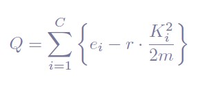
Where r is a resolution parameter (r > 0) that controls for the amount of communities: a greater resolution parameter gives more communities whereas a low resolution parameter fewer clusters. Since maximizing the modularity of a graph is an NP-hard problem, different heuristics are used, and Leiden has shown to outperform Louvain in this task both in terms of quality and speed [14]. However, users can choose to run the Louvain method instead by setting the parameter clustering="louvain" in the initialization of the Bootstrap object.
3.1) Most importantly, the authors comment that they found stronger expression of cell-type specific markers in the cells with high membership values - is it already a product of the Leiden algorithm that it weighs highly variable (thus cell-type specific) features higher - resulting in better prediction of cell-types for cells with strong cell-marker expression? It is important to make a description of transcriptional noise at this stage as it could be genome-wide or more specific to cell-type markers. Can authors provide any support that their method can capture both?
We agree with the reviewer that finding a stronger expression of cell-type markers in cells with high membership values is indeed something we expected. The graph representation of the dataset taken as input by Leiden is built after running highly variable gene detection and PCA. The neighbors of each cell are detected based on the expression of genes that are highly variable, as the reviewer pointed out, so genes that are differentially expressed between cells are more likely to contribute to the clusters found by Leiden.
Whether Scallop measures genome-wide or cell type-specific noise (or a mixture of both) is a very interesting question. Clusters in single-cell RNA sequencing datasets are often mainly driven by the presence/absence of a few cell type markers, rather than changes in expression levels of broader sets of genes. Moreover, it has been shown that single-cell RNAseq datasets generally preserve the same population structure even after data binarization [15]. This is a consequence of the sparsity of single-cell RNAseq datasets. In our case, any difference in expression between one cluster vs the rest of the cells in the dataset –be it the expression of a gene that was not detected in the rest of the cells or a higher expression of a gene whose presence is weaker in other clusters– will certainly have an impact on the output of every downstream analysis, from clustering to dimensionality reduction. The influence of the expression of cell type-specific markers on Scallop membership has been demonstrated in several analyses. First, the simulation where we measured the impact of removing the 10 most defining markers for a particular cell type on transcriptional noise measurements (included in the Figure 1 - Supplement 6 of the revised manuscript). Also, Figure 5 provides evidence that the differential expression of a handful of genes (in this case, genes coding for surfactant proteins) can have an impact on the clustering solutions obtained for a set of human alveolar macrophages, and this in turn influences the membership scores obtained with Scallop. In essence, Scallop merely provides a measure of the robustness of clustering at the single-cell level, so any type of transcriptional noise might have an impact on Scallop memberships, provided it is sufficiently strong to influence the output of the clustering algorithm used. In other words, the fact Scallop membership captures a mixture of both types of noise (genome-wide and that associated with cell type-specific markers) is a consequence of the influence both types of noise have on clustering.
4) The authors conclude that Scallop outperforms other methods through the analysis of biological data, where there is no positive and negative control. I suggest creating synthetic datasets (which could be based on real data), introducing different levels of noise artificially (considering biological constraints like max/min expression levels) and then testing the performance where the truth about each dataset is known. Otherwise, the definitions of noisy and stable cells, regardless of the method, are arbitrary.
Our initial focus was on biological datasets, were no positive and negative controls regarding transcriptional noise could be used, but we agree in the need of including an analysis using simulations on artificial datasets. We analyzed artificially generated datasets with known degrees of transcriptional noise in order to evaluate the performance of Scallop on a setting where the ground truth is known beforehand. The way we modeled transcriptional noise was by tuning the de.prob parameter, which determines the probability that a gene will be differentially expressed between clusters. The creation of these datasets is explained in detail in the Methods section of the revised manuscript, and specifically in the subsections Performance of Scallop and two DTC methods on four artificial datasets with increasing transcriptional noise. and Ability to detect noisy cells within cell types.
We have now included the following section in the Results:
"We compared the output of Scallop and two DTC methods (the whole transcriptome-based Euclidean distance to average cell type expression and the invariant gene-based Euclidean distance to average tissue expression) on four artificially generated datasets containing various levels of transcriptional noise. The analysis showed that Scallop, unlike DTC methods, was able to discern between the core transcriptionally stable cells within each cell type cluster from the more noisy cells that lie in between clusters (see Figure 1 - Supplement 1). We then compared one of the DTC methods to Scallop regarding their ability to detect noisy cells within each of the cell types, by plotting the top 10% noisiest and top 10% most stable cells and (see Figure 1 - Supplement 2A). Analyzing the distribution of noise values for each cell type separately revealed that Scallop can distinguish between clusters that mainly consist of transcriptionally stable cells from noisier clusters that do not have such a distinct transcriptional signature (Figure 1 - Supplement 2B."
Reviewer #3 (Public Review):
In this manuscript, Ibáñez-Solé et al aim to clarify the answer to a very basic and important question that has gained a lot of attention in the past ∼5 years due to fast-increasing pace of research in the aging field and development/optimization of single-cell gene expression quantification techniques: how does noise in gene expression change during the course of cellular/tissue aging? As the authors clearly describe, there have been multiple datasets available in the literature but one could not say the same for the number of available analysis pipelines, especially a pipeline that quantifies membership of single cells to their assigned cell type cluster. To address these needs, Ibáñez-Solé et al developed: 1. a toolkit (named Decibel) to implement the common methods for the quantification of age-related noise in scRNAseq data; and 2. a method (named Scallop) for obtaining membership information for single-cells regarding their assigned celltype cluster. Their analyses showed that previously-published aging datasets had large variability between tissues and datasets, and importantly the author’s results show that noise-increase in aging could not be claimed as a universal phenotype (as previously suggested by various studies).
We thank the reviewer for their positive assessment of the manuscript and their suggestions.
Comments:
1) In two relevant papers (doi.org/10.1038/s41467-017-00752-9anddoi.org/10.1016/j.isci. 2018.08.011), previous work had already shown what haploid/diploid genetic backgrounds could show in terms of intercellular/intracellular noise. Due to the direct nature of age/noise quantification in these papers, one cannot blame any computational pipeline-related issues for the ”unconventional” results. The authors should cite and sufficiently discuss the noise-related results of these papers in their Discussion section. These two papers collectively show how the specific gene, its protein half-life and ploidy can lead to similar/different noise outcomes.
We agree that we have failed to mention and sufficiently discuss the effects of measuring transcriptional noise from data generated via destructive experimentation, where no longitudinal analyses are possible. As aforementioned in the response to other reviewers, the body of literature on transcriptional noise is quite wide and based on heterogeneous assumptions. We have focused our efforts in measuring actual noise in scRNAseq aging datasets, which by definition imply sampling of different cells and thus make assumptions at the population level. We believe our results provide a different and interesting perspective into transcriptional noise and aging, but we agree with this reviewer in the need to discuss our findings in the context of other attempts to measure transcriptional noise in a more direct way. We have now included a brief discussion of the work by Sarnoski et al. and Liu et al.. This point is explained in more detail later in the letter.
2) While the authors correctly put a lot of emphasis on studying the same cell type or tissue for a faithful interpretation of noise-related results, they ignore another important factor: tracking the same cell over time instead of calculating noise from single-cell populations at supposedly-different age points. Obviously, scRNAseq cannot analyze the same cell twice, but inability to assess noise-in-aging in the same cell over time is still an important concern. Noise could/does affect the generation durations and therefore neighboring cells in the same cluster may not have experienced the same amount of mitotic aging, for example. Also, perhaps a cell has already entered senescence at early age in the same tissue. This caveat should be properly discussed.
The distinction between intrinsic and extrinsic noise and the impossibility to discern between the two in destructive experiments is a relevant point that we have now included in the Discussion (the newly added text is shown in italics):
"Transcriptional noise could be related to genomic instability [18], epigenetic deregulation [19, 20] or loss of proteostasis [21], all established hallmarks of aging. Some authors consider transcriptional noise to be a hallmark of aging in and of itself [22]. In any case, the origin of transcriptional noise is unclear, as it could arise from many different sources. Most importantly, it not possible to distinguish between intrinsic and extrinsic noise from a snapshot of cellular states, i.e., one cannot tell whether the observed differences between cells in a single-cell RNA experiment reflect time-dependent variations in gene expression or differences between cells across a population [23]. Interestingly, recent work by Liu et al. measuring intrinsic noise in S. cerevisiae showed that aging is associated with a steady decrease in noise, with a sudden increase in soon-to-die cells. Another longitudinal study found an increase extrinsic noise and a lack of change in intrinsic noise in diploid yeast [16]."
Regarding the caveat of cells of individuals in the Young groups showing signs of aging, we can only agree that this is correct: there will be cells sampled that already show signs of cellular damage in the absence of chronological aging. However this applies to every study of aging that samples cells in a destructive manner and it is generally assumed by the field that this is a discrete phenomenon that does not affect the overall results in a meaningful way.
3) Another weakness of this study is that the authors did not show the source/cause of decreasing/stable/increasing noise during aging. Understanding the source of loss of cell type identity is also important but this manuscript was about noise in aging, so it would have been nice if there could be some attempts to explain why noise is having this/that trend in differentially aged cell types in specific tissues.
The reviewer raises here a very important point that we would like to discuss in detail. The papers that we have re-analyzed generally assume that an increase in transcriptional noise and a loss in cell type identity are equivalent terms. However, as this reviewer points out, you could theoretically have cells that lose their cell type identity without a concomitant increase in transcriptional noise, for instance by a sharp decrease in a limited number of marker genes that collectively define that cell within a given cell type/cluster. Thus, transcriptional noise can certainly arise from different sources and several mechanisms have been proposed to explain its presence in the context of cellular aging. We agree with the reviewer that discussing how transcriptional noise could be related to aging is of interest to the readers. However, as pointed out in the responses to similar concerns by the other reviewers, our main finding is that we don’t detect meaningful and reliable increases in transcriptional noise associated with cell aging. Instead, what we see is a number of different technical and biological issues/phenomena that have been interpreted as transcriptional noise. We hope this reviewer will agree that the manuscript now presents a full and robust story and that finding the causes of up/down ”noise” trends in the different datasets may be more appropriately tackled by follow up studies.
4) In the discussion section, the authors say that ”Most importantly, Scallop measures transcriptional noise by membership to cell type-specific clusters which is a re-definition of the original formulation of noise by Raser and O’Shea.” It is not clear what the authors refer to by ”the original formulation of noise by Raser and O’Shea”. Intrinsic/extrinsic noise formulations?? Please be more specific.
We thank the reviewer for pointing this out, since we agree that the sentence needed to be reformulated for the sake of clarity. What we meant by the definition by Raser and O’Shea was ”the measured level of variation in gene expression among cells supposed to be identical”, which does not make any distinction between intrinsic and extrinsic noise. Since their definition is previous to the development of single-cell technologies, we meant to state our attempt to bring this classic concept to the context of single-cell RNAseq. Nowadays, cell clusters produced by a community detection algorithm are given cell type annotations depending on their expression of known cell type markers. What Scallop aims to measure is the extent of membership each individual cell has for their cluster as evidence of its transcriptional stability. In order to make this point more clear, we have now rewritten the paragraph as follows:
Most importantly, Scallop measures transcriptional noise by membership to cell type-specific clusters which is a re-definition of the original formulation of noise by Raser and O’Shea: measurable variation among cells that should share the same transcriptome. This is in stark contrast to measurements of noise including other phenomena (as demonstrated in Figure 5) by the distance-to-centroid methods prevalent in the literature.
References
[1] M. Alex Ascensión, Olga Ibáñez-Solé, Iñaki Inza, Ander Izeta, and Marcos J Araúzo-Bravo. Triku: A feature selection method based on nearest neighbors for single-cell data. GigaScience, 11, 2022. doi: 10.1093/gigascience/giac017.
[2] M. Ximerakis, S. L. Lipnick, B. T. Innes, S. K. Simmons, X. Adiconis, D. Dionne, B. A. Mayweather, L. Nguyen, Z. Niziolek, C. Ozek, V. L. Butty, R. Isserlin, S. M. Buchanan, S. S. Levine, A. Regev, G. D. Bader, J. Z. Levin, and L. L. Rubin. Single-cell transcriptomic profiling of the aging mouse brain. Nat Neurosci, 22(10), 2019. doi: https://doi:10.1038/s41593-019-0491-3.
[3] M. Enge, H. E. Arda, M. Mignardi, J. Beausang, R. Bottino, S. K. Kim, and S. R. Quake. Single-cell analysis of human pancreas reveals transcriptional signatures of aging and somatic mutation patterns. Cell, 171(2), 2017. doi: https://doi:10.1016/j.cell.2017.09.004.
[4] L. Solé-Boldo, G. Raddatz, and S. et al. Schütz. Single-cell transcriptomes of the human skin reveal age-related loss of fibroblast priming. Commun Biol, 3(188), 2020. doi: https://doi.org/10.1038/ s42003-020-0922-4.
[5] Jaime L. Schneider, Jared H. Rowe, Carolina Garcia-de Alba, Carla F. Kim, Arlene H. Sharpe, and Marcia C. Haigis. The aging lung: Physiology, disease, and immunity. Cell, 184(8):1990–2019, 2021. doi: 10.1016/j.cell.2021.03.005.
[6] Shuai Ma, Shuhui Sun, Jiaming Li, Yanling Fan, Jing Qu, Liang Sun, Si Wang, Yiyuan Zhang, Shanshan Yang, Zunpeng Liu, and et al. Single-cell transcriptomic atlas of primate cardiopulmonary aging. Cell Research, 31(4):415–432, 2020. doi: 10.1038/s41422-020-00412-6.
[7] I. Angelidis, L. M. Simon, and I. E. et al. Fernandez. An atlas of the aging lung mapped by single cell transcriptomics and deep tissue proteomics. Nature Communications, 2019. doi: https://doi.org/10. 1038/s41467-019-08831-9.
[8] Jonathan M. Raser and Erin K. O’Shea. Noise in gene expression: origins, consequences, and control. Science, 309(5743):2010–2013, 2005. doi: 10.1126/science.1105891.
[9] Michael B. Elowitz, Arnold J. Levine, Eric D. Siggia, and Peter S. Swain. Stochastic gene expression in a single cell. Science, 297:1183– 1186, 2002. doi: 10.1126/science.1070919.
[10] Peter S. Swain, Michael B. Elowitz, and Eric D. Siggia. Intrinsic and extrinsic contributions to stochasticity in gene expression. Proc Natl Acad Sci U S A., 99:12795–12800, 2002. doi: 10.1073/pnas.162041399.
[11] Alex Cagan, Adrian Baez-Ortega, Natalia Brzozowska, Federico Abascal, Tim H. H. Coorens, Mathijs A. Sanders, Andrew R. J. Lawson, Luke M. R. Harvey, Shriram Bhosle, David Jones, Raul E. Alcantara, Timothy M. Butler, Yvette Hooks, Kirsty Roberts, Elizabeth Anderson, Sharna Lunn, Edmund Flach, Simon Spiro, Inez Januszczak, Ethan Wrigglesworth, Hannah Jenkins, Tilly Dallas, Nic Masters, Matthew W. Perkins, Robert Deaville, Megan Druce, Ruzhica Bogeska, Michael D. Milsom, Björn Neumann, Frank Gorman, Fernando Constantino-Casas, Laura Peachey, Diana Bochynska, Ewan St. John Smith, Moritz Gerstung, Peter J. Campbell, Elizabeth P. Murchison, Michael R. Stratton, and Iñigo Martincorena. Somatic mutation rates scale with lifespan across mammals. Nature, 604: 517–524, 2022. doi: 10.1038/s41586-022-04618-z.
[12] Hamit Izgi, Dingding Han, Ulas Isildak, Shuyun Huang, Ece Kocabiyik, Philipp Khaitovich, Mehmet Somel, and Handan Melike Dönertas. Inter-tissue convergence of gene expression during ageing suggests age-related loss of tissue and cellular identity. eLife, 11, 2022. doi: 10.7554/eLife.68048.
[13] Vincent D Blondel, Jean-Loup Guillaume, Renaud Lambiotte, and Etienne Lefebvre. Fast unfolding of communities in large networks. Journal of Statistical Mechanics: Theory and Experiment, 2008(10): P10008, oct 2008. doi: 10.1088/1742-5468/2008/10/p10008. URL https://doi.org/10.1088/ 1742-5468/2008/10/p10008.
[14] V. A. Traag, L. Waltman, and N. J. van Eck. From louvain to leiden: guaranteeing well-connected communities. Scientific Reports, 9, 2019. doi: https://doi.org/10.1038/s41598-019-41695-z.
[15] Peng Qiu. Embracing the dropouts in single-cell rna-seq analysis. Nature Communications, 11(1), 2020. doi: 10.1038/s41467-020-14976-9.
[16] Ethan A. Sarnoski, Ruijie Song, Ege Ertekin, Noelle Koonce, and Murat Acar. Fundamental characteristics of single-cell aging in diploid yeast. iScience, 7:96–109, 2018. doi: 10.1016/j.isci.2018.08.011.
[17] Ping Liu, Ruijie Song, Gregory L. Elison, Weilin Peng, and Murat Acar. Noise reduction as an emergent property of single-cell aging. Nature Communications, 8(1), 2017. doi: 10.1038/s41467-017-00752-9.
[18] Jan Vijg. From dna damage to mutations: All roads lead to aging. Ageing Res Rev., 68(101316), 2021. doi: 10.1016/j.arr.2021.101316.
[19] Yuancheng Lu, Benedikt Brommer, Xiao Tian, Anitha Krishnan, Margarita Meer, Chen Wang, Daniel L. Vera, Qiurui Zeng, Doudou Yu, Michael S. Bonkowski, Jae-Hyun Yang, Songlin Zhou, Emma M. Hoffmann, Margarete M. Karg, Michael B. Schultz, Alice E. Kane, Noah Davidsohn, Ekaterina Korobkina, Karolina Chwalek, Luis A. Rajman, George M. Church, Konrad Hochedlinger, Vadim N. Gladyshev, Steve Horvath, Morgan E. Levine, Meredith S. Gregory-Ksander, Bruce R. Ksander, Zhigang He, and David A. Sinclair. Reprogramming to recover youthful epigenetic information and restore vision. Nature, 588(7836):124–129, 2020. doi: 10.1038/s41586-020-2975-4.
[20] Giorgio Oliviero, Sergey Kovalchuk, Adelina Rogowska-Wrzesinska, Veit Schwämmle, and Ole N. Jensen. Distinct and diverse chromatin proteomes of ageing mouse organs reveal protein signatures that correlate with physiological functions. eLife, 11(e73524), 2022. doi: 10.7554/eLife.73524.
[21] Jingyi Li, Yuxuan Zheng, Pengze Yan, Moshi Song, Si Wang, Liang Sun, Zunpeng Liu, Shuai Ma, Juan Carlos Izpisua Belmonte, Piu Chan, Qi Zhou, Weiqi Zhang, Guang-Hui Liu, Fuchou Tang, and Jing Qu. A single-cell transcriptomic atlas of primate pancreatic islet aging. Natl Sci Rev., 8(2): nwaa127, 2020. doi: 10.1093/nsr/nwaa127.
[22] Alexander R. Mendenhall, George M. Martin, Matt Kaeberlein, and Rozalyn M. Anderson. Cellto-cell variation in gene expression and the aging process. Geroscience, 43(1):181–196, 2021. doi: 10.1007/s11357-021-00339-9.
[23] Lucy Ham, Marcel Jackson, and Michael PH Stumpf. Pathway dynamics can delineate the sources of transcriptional noise in gene expression. eLife, 10, 2021. doi: 10.7554/elife.69324.
Author Response
Reviewer #1 (Public Review):
Bice et al. present new work using an optogenetics-based stimulation to test how this affects stroke recovery in mice. Namely, can they determine if contralateral stimulation of S1 would enhance or hinder recovery after a stroke? The study provides interesting evidence that this stimulation may be harmful, and not helpful. They found that contralesional optogenetic-based excitation suppressed perilesional S1FP remapping, and this caused abnormal patterns of evoked activity in the unaffected limb. They applied a network analysis framework and found that stimulation prevented the restoration of resting-state functional connectivity within the S1FP network, and resulted in limb-use asymmetry in the mice. I think it's an important finding. My suggestions for improvement revolve around quantitative analysis of the behavior, but the experiments are otherwise convincing and important.
Thank you for the positive feedback regarding our work.
Other comments - Data and paper presentation:
1) Figure 1A is misleading; it appears as if optogenetic stimulation is constant (which indeed would be detrimental to the tissue). Also, the atlas map overlaps color-wise with conditions; at a glance it looks like the posterior cortex might be stimulated; consider making greyscale?
We have updated Figure 1A to address these concerns.
Reviewer #2 (Public Review):
These studies test the effect of stimulation of the contralateral somatosensory cortex on recovery, evoked responses, functional interconnectivity and gene expression in a somatosensory cortex stroke. Using transgenic mice with ChR2 in excitatory neurons, these neurons are stimulated in somatosensory cortex from days 1 after stroke to 4 weeks. This stimulation is fairly brief: 3min/day. Mice then received behavioral analysis, electrical forepaw stimulation and optical intrinsic signal mapping, and resting state MRI. The core finding is that this ChR2 stimulation of excitatory neurons in contralateral somatosensory cortex impairs recovery, evoked activity and interconnectivity of contralateral (to the stimulation, ipsilateral to the stroke) cortex in this localized stroke model. This is a surprising result, and resonates with some clinical findings, and a robust clinical discussion, on the role of the contralateral cortex in recovery. This manuscript addresses several important topics. The issue of brain stimulation and alterations in brain activity that the studies explore are also part of human brain stimulation protocols, and pre-clinical studies. The finding that contralateral stimulation inhibits recovery and functional circuit remapping is an important one. The rsMRI analysis is sophisticated.
Thank you for the supportive comments regarding our manuscript
Concerns:
1) The gene expression data is to be expected. Stimulation of the brain in almost any context alters the expression of genes.
We agree with the reviewer that stimulation of the brain is expected to broadly alter gene expression. However, in this set of studies, we examined a subset of genes that are of particular interest in neuroplasticity, and compared expression in ipsi-lesional vs. contra-lesional cortex in the presence or absence of contralesional stimulation during the post stroke recovery period. Genes like Arc, for example, have been shown by our group to be necessary for perilesional plasticity and recovery (Kraft, et al., Science Translational Medicine, 2018). The finding that validated plasticity genes are suppressed by contralesional stimulation is consistent with the central finding that contralesional stimulation suppresses the recovery of normal patterns of brain organization and activity. Importantly, there were also genes associated with spontaneous recovery that were unaltered or increased by contra-lesional brain stimulation. While these data do not provide causal associations, they may prove to be useful for developing hypotheses regarding molecular mechanisms involved in spontaneous brain repair for future studies.
In light of the reviewer’s comment, we have altered text throughout to not focus on specific directionality of transcripts. Instead, we indicate that relevant transcript changes are those that are altered in association with spontaneous recovery, and which are altered in the opposite direction with contralesional brain stimulation.
Minor points.
1) Was the behavior and the functional imaging done while the brain was being stimulated?
We have updated the methods (page 17) to clarify that the only experiments during which the photostimulus occurred during neuroimaging are reported in new Figure 6, and to clarify that photostimulation did not occur during the behavioral tests of asymmetry.
2) It would be useful to understand what is being stimulated. The stimulation method is not described. Is an entire cortical width of tissue stimulated, and this is what is feeding back onto the contralateral cortex? Or is this stimulation mostly affecting excitatory (CaMKII+) cells in upper or lower layers? This will be important to be able to compare to the Chen et al study that gave rise to the stimulation approach here. This gets to the issue of the circuitry that is important in recovery, or in inhibiting recovery. One might answer this question by doing the stimulation and staining tissue for immediate early gene activation, to see the circuits with evoked activity. Also, the techniques used in this study could be applied with OIS or rsMRI during stimulation, to determine the circuits that are activated.
We have clarified the stimulation protocol in response to Essential point 2.2. Due to light scattering and appreciable attenuation of 473nm in brain tissue, only ~1% of photons penetrate to a depth of 600 microns. Experimentally, this provides superficial-layer specificity to Layer 2/3 Camk2a cells (https://doi.org/10.1016/j.neuron.2011.06.004)
To answer the question of what circuits are affecting recovery, we performed 2 sets of additional experiments – Experiment 1: OISI during photostimulation before and after photothrombosis, and Experiment 2: tissue staining for IEG expression (cFOS). We describe each below:
Experiment 1 New results are included from 16 Camk2a-ChR2 mice (Results, page 10-11; Methods, page 18) and reported as new Figure 6. Similar to the previously reported experiments, all mice were subject to photothrombosis of left S1FP, half of which received interventional optogenetic photostimulation beginning 1 day after photothrombosis (+Stim) while the other half recovered spontaneously (-Stim). To visualize in real time whether contralesional photostimulation differentially affected global cortical activity in these 2 groups, concurrent awake OISI during acute contralesional photostimulation was performed in +Stim and –Stim groups before, 1, and 4 weeks after photothrombosis. At baseline, all mice exhibited focal increases in right S1FP activity during photostimulation that spread to contralateral (left) S1FP and other motor regions approximately 8-10 seconds after stimulus onset. While activity increases within the targeted circuit, subtle inhibition of cortical activity can also be observed in surrounding non-targeted cortices. Thus, activity both increases and decreases in different cortical regions during and after optogenetic stimulation of the right S1FP circuit. Of note, regions that are inhibited by S1FP stimulation show more pronounced decreases in activity in +Stim mice at 1 and 4 weeks compared to baseline and were significantly larger in +Stim mice compared to –Stim mice. We conclude that focal stimulation of contralesional cortex results in significant, widespread inhibitory influences that extend well beyond the targeted circuit.
Experiment 2 For experiment 2, we hypothesized that IEG expression would increase in photostimulated regions, cortical regions functionally connected to targeted areas, and potentially deeper brain regions. For the IEG experiments, healthy ChR2 naïve animals (C57 mice) or CamK2a-ChR2 mice were acclimated to the head-restraint apparatus described in the manuscript used for photostimulation treatment. Once trained, awake mice were subject to the same photostimulus protocol as described in the manuscript applied to forepaw somatosensory cortex in the right hemisphere. After stimulation, mice were sacrificed, perfused, and brains were harvested for tissue slicing and immunostaining for cFOS. Tissue slices containing right and left primary forepaw somatosensory cortex and primary and secondary motor cortices (+0.5mm A/P) or visual cortex (-2.8mm A/P) were examined for cFOS staining and compared across groups.
Below is a summary table of our findings, and representative tissue slices. While c-FOS IHC was successful, results are not consistent with expectations from the mouse strains used. Only 1 ChR2+ mouse exhibited staining patterns consistent with local S1FP photostimulation, while expression in ChR2- mice was more variable, and in some instances exhibits higher expression in targeted circuits compared to ChR2+ mice. It is possible that awake behaving mice already exhibit high activity in sensorimotor cortex at rest, which might obscure changes specific to optogenetic photostimulation. Regardless, because the tissue staining experiments were inconclusive in healthy animals, we did not proceed with further experiments in the stroke groups, and do not report these findings in the manuscript.
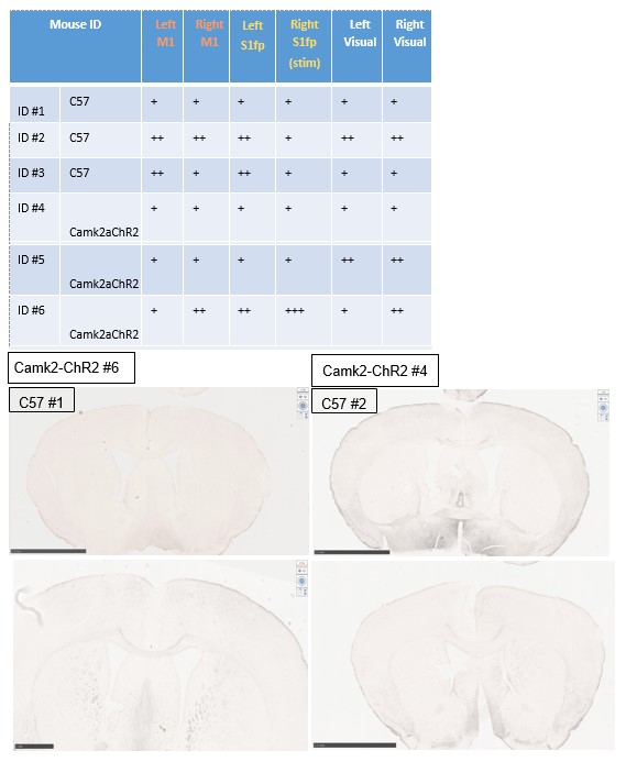
3) Also, it is possible that contralateral stimulation is impairing recovery, not through an effect on the contralateral cortex (the site of the stroke), but on descending projections, or theoretically even through evoking activity or subclinical movement of the contralateral limb (ipsilateral to the stroke). By more carefully mapping the distribution of the activity of the stimulated brain region, and what exactly is being stimulated, these issues can be explored.
The reviewer raises an excellent point. We have added to the “Limitations and Future work” section of the Discussion on pages 15-16
Author Response:
Evaluation Summary:
This study, which will be of interest to neuroscientists in the fields of learning and memory, somatosensation, and motor behavior, uses systems neuroscience tools to expand our view how the postero-medial (POm) nucleus of the thalamus contributes to goal-directed behavior. The reviewers suggested additional ontogenetic experiments to clarify the nature and specificity of those roles. They also indicated that certain alternative explanations to the experimental observations could be addressed for a more balanced presentation and interpretation of the results.
We thank the editors and reviewers for their constructive comments. We have now performed additional analysis and revised the text which we believe has improved the manuscript.
Reviewer #1 (Public Review):
1) Fig 1 - Supp 1 suggests that virus expression was always limited to POm. Drawing borders expressing areas from epifluorescence images is probably very dependent on imaging parameters. The Methods indicate that the authors scaled so that no pixels were saturated. This could mean that there was some weak expression of GCaMP6f or ArchT outside of POm. As I understand it, the authors set exposure/gains by the brightest points in the image. The limited extent of the infection in the figures might just reflect its center, which is brightest, rather than its full extent. If there were GCaMP or ArchT in VPL, some results would need to be reinterpreted.
We agree with the reviewer that the determined expression areas are dependent on imaging parameters, however, we are confident that the virus expression used for analysis in this study are confined to the POm. In this study, our analysis of targeting of POm is three-fold. First, we optimized the volume of virus loaded to the minimum necessary to observe POm projections in S1 (a single targeted injection of 60 nl). Second, we analyzed the fluorescence spread using fluorescence microscopy after every experiment. We set exposure to use the full dynamic range of the image as previously described (Gambino et al., 2014). Occasionally, the virus spread to the adjacent VPM nucleus and this was easily recognizable by the characteristic VPM projections with the barrels of the barrel cortex. These animals were excluded from this study and not further analyzed. The VPL nucleus is located further caudally in respect to the VPM and again, we were able to identify if the virus has spread to this nucleus via posthoc fluorescence microscopy. These animals were excluded from this study and not further analyzed. We note that our stereotaxic injections were not flawless and the virus occasionally spread along the injection pipette track and into high-order visual thalamic nuclei LP and LD, superficial to POm. This is shown in Figure 1. These two nuclei, however, do not target S1 (Kamishina et al., 2009; van Groen and Wyss, 1992) and were therefore not imaged within our study. Third, we analyze the projection profile in FPS1 to ensure that it corresponds to the projection profile of POm and not VPL. If there is fluorescence in non-targeted areas, then the experiments were excluded from analysis.
An additional degree of precision is offered by our imaging and optogenetic strategy. Calcium imaging was performed in layer 1 which is targeted by POm (Meyer et al., 2010), and not VPL which targets layer 4. Therefore, spillover into VPL would not influence our imaging results as we only image axons in layer 1 which is targeted by POm. Furthermore, during the optogenetic experiments, the fiber optic was targeted to the POm (not the VPL), thus providing a secondary POm localization of the photo-inhibited region. This is now discussed in the revised manuscript.
2) Calcium responses are weaker during the naïve state than the expert state (Fig.1D,E), similar to the start of the reversal training (Fig.4G,H). If POm encodes correct actions, why is there any response at all in naïve mice? Is that not also a sign of stimulus encoding? Might there be another correlate of correctness with regard to the task, such as an expert mouse holding their paw more firmly or still on the stimulating rod? This could alter the effective stimulus or involve different motor signals to POm.
We agree with the reviewer that the POm is encoding the stimulus in the naïve state. This is evident in our study, and others, which show that the POm increases activity during sensory input in naïve mice. In the expert state, stimulus encoding may also be performed by a subset of POm axons, however, our findings show that, overall, there is a significant increase in the POm activity which is dependent on the behavioral performance (HIT, MISS), and not on the presentation of the stimulus. This is not due to licking motion as there was similar POm activity during the action and suppression tasks which involved licking and not licking for reward (Figure 3E). Furthermore, all experiments were monitored online via a behavioral camera to examine the location of the forepaw on the stimulus during all trials, and trials where the paw was not clearly resting on the stimulating rod were excluded from analysis. However, we cannot rule out that non-detectable changes in postures/paw grip may occur which may alter the effectiveness of the stimulus. This is now discussed in the revised manuscript.
3) The authors are rightly concerned that licking might contribute to POm activity and expend some good effort checking this. The reversal is a good control, but doesn't produce identical POm activity. The other licking analyses, while good, did not completely rule out licking effects. First, lines 110-111 state "…as there was no correlation between licking frequency and POm axonal activity (Figure 1I)", but Fig.1I doesn't seem to support that statement. Second, the authors analyze isolated spontaneous licks, but these probably involve less licking and less overall motion than during a real response.
We thank the reviewer for acknowledging the effort we made to assess the influence of licking behavior on POm axonal activity. We now include a more direct analysis in the revised manuscript illustrating the relationship between the licking response and POm activity. This analysis shows there is no correlation between licking and POm axonal activity (linear regression, p = 0.9228), further suggesting that POm axonal activity is not simply due to licking behavior.
4) Many figures (Fig.1F, 2B, 3C, 4C) make it apparent that a population of axons respond very early to the stimulus itself. I understand the authors point that many of their analyses show that on average the axons are not strongly modulated by this stimulus, but this is not true of every axon. Either some of these axons are coming from cells outside of POm (see #1) or some POm cells are stimulus driven. In either case, if some axons are strongly stimulus driven, the activity of these axons will correlate with correct choices. The stimulus and correct choices are themselves highly correlated because the animals perform so well. I do not understand how stimulus encoding and choice encoding can be disentangled by either behavior or the two behaviors in comparison. Simple stimulus encoding might be further modulated by arousal or reward expectation that increases with task learning (see #6).
In this study, we are able to disentangle stimulus encoding and choice encoding by comparing the POm axonal activity with the different behavioral performance (HIT or MISS). Here, the same stimulus is always presented (tactile, 200 Hz), however, the mouse response differs. Despite receiving the same tactile stimulus, POm signaling in forepaw S1 is significantly increased during correct HIT trials compared with MISS trials in both the action and suppression task. Therefore, we do not believe POm axonal activity is predominantly encoding sensory information in this task. We agree with the reviewer that individual POm axons are heterogenous and a subset of axons may respond to the sensory stimulus during the behavior. We now state this in the revised manuscript. However, if some axons are strongly stimulus driven, the activity of these axons should correlate with both correct and incorrect choices as the same stimulus is also delivered during MISS trials. We now highlight this in the revised manuscript.
Simple stimulus encoding might be further modulated by arousal or reward expectation that increases with task learning. In our study, the increase in POm activity during HIT behaviour was not due to elevated task engagement as, despite similar levels of arousal (Figure 4B), POm activity in expert mice differed in comparison to chance performance (switch behaviour; Figure 4G, H). This is now discussed in detail in the revised manuscript.
5) I was unable to understand the author's conclusion about what POm is doing. They use terms like "behavioral flexibility" to describe its purpose, but the connection of this term to POm is not explained. Is a role as a flexibility switch really supported? Why does S1 need POm to signal a correct choice? Fig.6 did not seem helpful here. Couldn't S1 just detect the stimulus on its own and transmit consequent signals to wherever they need to be to generate behavior?
We have now revised the manuscript and clearly define behavioral flexibility and to improve the clarity of our conclusions. We believe that S1 needs POm to signal a correct choice as behavior needs to be dynamically modulated at all times. If S1 simply detected the stimulus on its own and transmitted a consequent signals to generate behavior, then important modulatory processes that lead to dynamic changes in behavior would not be processed. Along with other feedback projections, the POm targets the upper layers of the cortex, whereas external sensory information targets the layer 4 input layer. At the level of a single pyramidal neuron, this means POm input lands on the tuft dendrites whereas external sensory information lands on the proximal basal dendrites. This segregation of input provides a great cellular mechanism for increasing the computational capabilities of neurons. Since the POm is most active in the expert state during correct behavior, we believe the POm plays a vital role in providing behaviorally relevant information. Our findings illustrate that the POm is simply not conveying a ‘Go’ signal as POm activity was not increased during correct behavior in chance performance.
6) Arousal or reward expectation may be better explanations than flexibility. Lines 323-324 say that POm activity increased with pupil diameter normally but reversed during reward delivery. Which data support this statement? With regards to pupil, the Results only seem to indicate that there is no difference in diameter between the two conditions (expert and 50% chance) using 3 bins of data. However, I could not find the time windows used for computing these. Pupil is known to be lagged and the timing could be critical.
The statement that ‘POm activity increased with pupil diameter normally but reversed during reward delivery’ stems from data illustrated in Figure 1I and 3B. For space and flow of the manuscript, we weren’t able to show them on the same graph as per below. Here, you can see that during reward (blue), POm activity decreased compared to response (green) whereas the pupil diameter was maximum during reward delivery. We now include more information in the methods regarding pupil tracking (see line 908 to 916, Data analysis and statistical methods; Pupil tracking).
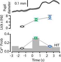
7) There are other possible interpretations of the results when the authors target POm for optogenetic suppression (around lines 246-248). The effects here are also consistent with preventing tonic and evoked POm activity from reaching lots of target structures other than S1: S2, PPC, motor cortex, dorsolateral striatum, etc. Maybe one of these cannot respond to the stimulus as well and Hits decrease?
We now include a discussion in the revised manuscript that ‘since the POm targets many cortical and subcortical regions (Alloway et al., 2017; Oh et al., 2014; Trageser and Keller, 2004; Yamawaki and Shepherd, 2015), target-specific photo-inhibition is required to illustrate which POm projection pathway specifically influences goal-directed behavior.’
8) Line 689. What alerts the mouse that a catch trial is happening? Is there something like an audio cue for onset of stimulus trials and catch trials? If there is no cue, wouldn't mice be in a different behavioral state during catch trials than during stimulus trials? The trial types could differ by more than the presence of the stimulus.
There is broadband noise during the trial that acts as a cue. This is detailed in the methods and text.
Reviewer #2 (Public Review):
In this manuscript, D LaTerra et al explored the function of POm neurons during a tactile-based, goal-directed reward behavior. They target POm neurons that project to forepaw S1 and use two-photon Ca2+imaging in S1 to monitor activity as mice performed a task where forepaw tactile stimulation (200 Hz, 500 ms) predicted a reward if mice licked at a reward port within 1.5 seconds. If mice did not lick, there was a time-out instead of a reward. The authors found that POm-S1 axons showed enhanced responses during the baseline period, the response window after the cue, and during reward delivery. They then showed that a subset of neurons were active during the response window during correct trials when the tactile stimulus served as a cue, but not on catch trials where animals spontaneously licked for a reward.
They then showed that POm axonal activity in S1 increased during the response window for "HIT" trials where animals correctly responded to the tactile stimulus with licking but the activity was less during "MISS" trials where animals did not respond. In order to probe whether this activity in the response window was being driven by motor activity, they designed a suppression task in which animals had to learn to suppress licking in response to the tactile stimulus in order to the receive a reward. POm neurons also showed increased activity during the response window even though action was being suppressed. However, this activity was less than during the action task. Thus, although POm activity is not encoding action, its activity is significantly different during an action-based task than an action suppression one. They then analyzed calclium activity during the training period between the action task and the suppression task in which animals were learning the new contingency and were not performing as experts. In this non-expert context there was not a difference between in POm axonal activity between "HIT" and "MISS" trials.
Lastly, they used ArchT to inhibit POm cell body activity during the tactile stimulus and response window of some trials and showed that they reduced performance during the trials when light was on.
Altogether, this paper provides evidence that POm neurons are not simply encoding sensory information. They are modulated by learning and their activity is correlated to performance in this goal-directed task. However, the actual role of the POm input to S1 is not discernable from the current experiments. Subsets of neurons show significant activity during the response window as well as reward. In addition, the role of this input is different during the switch task than during expert performance. There are a number of outstanding questions, which, if answered, would help to directly define the role of these neurons in this specific paradigm. For instance, the authors record specifically from POm axons in S1. How distinct is this activity from other neurons in the POm? Some POm neurons still show significant activity during MISS trials. Do these neurons have a different function than those that show a preferential response during HIT trials? Does POm activity during the switch task, which has a component of extinction training, differ from when the animals are first learning the action-based task? Likewise, are the same neurons that acquire a response during the initial learning of the action-based task, the same neurons that are responding during the action suppression task?
The authors provide great evidence that POm neurons that project to the S1 do not simply encode sensory information or actions, but are instead signaling during correct performance. However, inhibition of cell bodies did not dramatically effect performance and it is still unclear what role this circuit actually plays in this behavior. Finer-tuned optogenetic experiments and analysis of cell bodies within POm may provide greater details that will help define this circuit's role.
We thank the reviewer for their comments. We have now revised the manuscript to clearly state the role of the POm during the goal-directed behavioral tasks used in this study. We have provided more information regarding the range of activity patterns in POm axons within S1.
The POm contains a heterogenous population of neurons and since it projects to multiple cortical and subcortical regions, the activity of POm axonal projections in S1 may indeed be different to other projection targets.
The activity of POm axons during MISS behavior may have a different function than those that show a preferential response during HIT trials, however, this evoked rate is not significantly different to baseline and therefore is hard to differentiate from spontaneous activity (see Figure 2). Furthermore, the evoked rate of POm activity during the switch task is not significantly different compared to naïve mice (p = 0.159; Kruskal-Wallis test). This information is now included in the manuscript.
It is unknown whether the same neurons that acquire a response during the initial learning of the action-based task are the same neurons that are responding during the action suppression task as we were unable to conclusively determine whether or not the same POm axons were imaged in the different protocols.
Reviewer #3 (Public Review):
In their paper "Higher order thalamus flexibly encodes correct goal-directed behavior", LaTerra et al. investigate the function of projections from the thalamic nucleus POm to primary somatosensory cortex (S1) in the performance of goal-directed behaviors. The authors performed in vivo calcium imaging of POm axons in layer 1 of the forepaw region of S1 (fpS1) to monitor the activity of POm-fpS1 projections while mice performed a tactile detection task. They report that the activity of POm-fpS1 axons on successful ('hit') trials was increased in trained mice relative to naïve mice. Additionally, the authors used an action suppression variant of the task to show that POm-fpS1 axon activity was higher on successful trials over unsuccessful ('miss') trials regardless of the correct motor response required. During transition between task conditions, when mice perform at chance levels, the increase of POm-fpS1 activity during correct trials is no longer seen. Finally, the authors use inhibitory optogenetic tools to suppress POm activity, revealing a modest suppression in behavioral success. The authors conclude from these data that POm-fpS1 axons preferentially "encode and influence correct action selection" during tactile goal-oriented behavior.
This study presents several interesting findings, particularly with respect to the change in activity of POm-fpS1 axons during successful execution of a trained behavior. Additionally, the similarity in responses of POm-fpS1 on both the 'goal-directed action' and 'action suppression' tasks provides convincing evidence that POm-fpS1 activity is not likely to encode the motor response. Overall, these results have important implications for how activity in higher order thalamic nuclei corresponds to learning a sensorimotor behavior, and the authors use several clever experiments to address these questions. Yet, the major claim that POm encodes 'correct performance' should be defined more clearly. As is, there are alternative explanations that could be raised and should be discussed in more depth (Points 1), especially as it relates to any causal role the authors ascribe to POm (Point 2). In addition some clarification as to which types of signals (i.e. frequency of active axons vs. amplitude of signal in the active axons) the authors feel are most informative would be helpful (Point 3).
We thank the reviewer for their helpful comments and assessment of our study. We have now addressed all comments and revised the manuscript accordingly.
1) The authors argue that POm activity reflects 'correct task performance' and that the increased activity of POm-fpS1 axons in the response epoch is not due to sensory encoding. An alternative explanation is that POm-fpS1 axons do convey sensory information, and these connections are facilitated with learning - meaning the activity of pathways conveying sensory signals that are correlated with task success could be facilitated with training, and this facilitation could be disrupted during the switching task. In this sense, the activity profiles do not encode 'correct action' per se, but rather represent the sensory responses whose correlation to rewarded action have been reinforced with training (which would also be a very interesting finding). This would be quite distinct from the "cognitive functions" they ascribe to this pathway (line 341). It might have helped to introduce a delay period in between the sensory stimulus and response epoch to try to distinguish responses that encode information about the sensory stimulus from those that might be involved in encoding task performance. However, as is, it is difficult to distinguish between these two scenarios with this data, and thus the interpretations the authors present could be rephrased with alternatives discussed in more depth.
Based on multiple findings within this study, we suggest that the POm does not predominantly encode sensory information. This is most evident when comparing POm activity during correct (HIT) and incorrect (MISS) behavior in both the action and suppression tasks. As shown in Figures 2 and 3, there is a considerable difference in activity during correct (HIT) and incorrect (MISS) trials, even though the same stimulus was delivered in both trial types. This finding suggests that POm axons do not convey sensory information which is facilitated with learning as, if this were true, it could be expected that HIT and MISS responses would be similarly increased in expert (HIT and MISS) compared to naïve mice. This is now discussed in detail in the revised manuscript.
We agree that it would have been beneficial to separate the stimulus from the response period in the behavioral paradigm. However, to avoid engaging working memory, we did not wish to enforce a delay period in this study. We have, in another study, enforced a short delay period (500 ms) between the stimulus and response epoch. Here, the evoked rate of POm axonal activity in expert mice was three-fold greater in the (now clearly separated) response epoch compared to the stimulus epoch (0.30 ± 0.02 vs. 0.099 ± 0.01, n = 196 dendrites; p < 0.0001; Wilcoxon matched-pairs signed rank test). Although out of the scope of this study, these unpublished results provides further confirmation and confidence in the analysis performed and conclusions made in this study.
2) Similarly, while the authors attempt to establish a causal role for POm in task performance by optogenetically inhibiting POm during the response epoch, the results are also consistent with a deficit in sensory processing, and cannot be interpreted strictly as a disruption of the encoding of 'correct action' task performance signals. Furthermore, these perturbation studies do not demonstrate that the POm-fpS1 projections they are studying are implicated in the modest behavioral deficits. As the authors state, POm projects to many targets (lines 63-66), and similar sensory-based, goal-directed behaviors do not require S1 (lines 302-305). In light of these points, some of the statements ascribing a causal role for these projections in task success could be rephrased (e.g. line 33 "to encode and influence correct action selection", line 252 "a direct influence", line 340 "plays an active role during correct performance").
We agree that the decrease in correct performance during optogenetic inhibition of POm cell bodies may also be explained by a deficit in sensory processing. However, in this study, we went to great lengths to illustrate that the POm is encoding correct action, and not sensory information (detailed in response to 1). This is further expanded upon in the revised manuscript. We also agree that the perturbation studies do not directly demonstrate that the POm to S1 projections are driving the behavioral deficits. We therefore only refer to the POm itself when discussing the influence on behavior and we have now revised the manuscript accordingly.
3) Event amplitude and probability were both quantified, but were not consistently reported throughout the manuscript and figures. For example, Figure 1 reports both probability and amplitude (Figure 1G and H), whereas Figure 2 only reports probability. Thus, it was not always clear as to whether the authors were ascribing biological significance to one or both of these measures, given that in some cases differences were found in one and not the other, and which of the measures were reported was occasionally switched. It would be helpful for the authors to clarify the significance they assign to each measure, and report both measures side by side for all experiments if they interpret them both as relevant.
We thank the reviewer for this observation and have now included a statement discussing the reporting of Ca2+ transient probability and/or amplitude in the methods. Throughout the Figures, we typically illustrated probability of an evoked transient as this is a reliable measure which was dramatically altered within this study. We now report the Ca2+ transient peak amplitudes during HIT and MISS trials for direct comparison of both measures (Figure 2).
Author Response
Reviewer #1 (Public Review):
It is now widely accepted that the age of the brain can differ from the person's chronological age and neuroimaging methods are ideally suited to analyze the brain age and associated biomarkers. Preclinical studies of rodent models with appropriate neuroimaging do attest that lifestyle-related prevention approaches may help to slow down brain aging and the potential of BrainAGE as a predictor of age-related health outcomes. However, there is a paucity of data on this in humans. It is in this context the present manuscript receives its due attention.
Comments:
1) Lifestyle intervention benefits need to be analyzed using robust biomarkers which should be profiled non-invasively in a clinical setting. There is increasing evidence of the role of telomere length in brain aging. Gampawar et al (2020) have proposed a hypothesis on the effect of telomeres on brain structure and function over the life span and named it as the "Telomere Brain Axis". In this context, if the authors could measure telomere length before and after lifestyle intervention, this will give a strong biomarker utility and value addition for the lifestyle modification benefits. 2) Authors should also consider measuring BDNF levels before and after lifestyle intervention.
Response to comments 1+2: we agree that associating both telomere length and BDNF level with brain age would be interesting and relevant. However, we did not measure these two variables. We would certainly consider adding these in future work. Regarding telomere length, we now include a short discussion of brain age in relation to other bodily ages, such as telomere length (Discussion section):
“Studying changes in functional brain aging is part of a broader field that examines changes in various biological ages, such as telomere length1, DNA methylation2, and arterial stiffness3. Evaluating changes in these bodily systems over time allows us to capture health and lifestyle-related factors that affect overall aging and may guide the development of targeted interventions to reduce age-related decline. For example, in the CENTRAL cohort, we recently reported that reducing body weight and intrahepatic fat following a lifestyle intervention was related to methylation age attenuation4. In the current work, we used RSFC for brain age estimation, which resulted in a MAE of ~8 years, which was larger than the intervention period. Nevertheless, we found that brain age attenuation was associated with changes in multiple health factors. The precision of an age prediction model based on RSFC is typically lower than a model based on structural brain imaging5. However, a higher model precision may result in a lower sensitivity to detect clinical effects6,7. Better tools for data harmonization among dataset6 and larger training sample size5 may improve the accuracy of such models in the future. We also suggest that examining the dynamics of multiple bodily ages and their interactions would enhance our understanding of the complex aging process8,9. “
And
“These findings complement the growing interest in bodily aging indicated, for example, by DNA methylation4 as health biomarkers and interventions that may affect them.”
Reviewer #2 (Public Review):
In this study, Levakov et al. investigated brain age based on resting-state functional connectivity (RSFC) in a group of obese participants following an 18-month lifestyle intervention. The study benefits from various sophisticated measurements of overall health, including body MRI and blood biomarkers. Although the data is leveraged from a solid randomized control set-up, the lack of control groups in the current study means that the results cannot be attributed to the lifestyle intervention with certainty. However, the study does show a relationship between general weight loss and RSFC-based brain age estimations over the course of the intervention. While this may represent an important contribution to the literature, the RSFC-based brain age prediction shows low model performance, making it difficult to interpret the validity of the derived estimates and the scale of change. The study would benefit from more rigorous analyses and a more critical discussion of findings. If incorporated, the study contributes to the growing field of literature indicating that weight-reduction in obese subjects may attenuate the detrimental effect of obesity on the brain.
The following points may be addressed to improve the study:
Brain age / model performance:
1) Figure 2: In the test set, the correlation between true and predicted age is 0.244. The fitted slope looks like it would be approximately 0.11 (55-50)/(80-35); change in y divided by change in x. This means that for a chronological age change of 12 months, the brain age changes by 0.11*12 = 1.3 months. I.e., due to the relatively poor model performance, an 80-year-old participant in the plot (fig 2) has a predicted age of ~55. Hence, although the age prediction step can generate a summary score for all the RSFC data, it can be difficult to interpret the meaning of these brain age estimates and the 'expected change' since the scale is in years.
2) In Figure 2 it could also help to add the x = y line to get a better overview of the prediction variance. The estimates are likely clustered around the mean/median age of the training dataset, and age is overestimated in younger subs and overestimated in older subs (usually referred to as "age bias"). It is important to inspect the data points here to understand what the estimates represent, i.e., is variation in RSFC potentially lost by wrapping the data in this summary measure, since the age prediction is not particularly accurate, and should age bias in the predictions be accounted for by adjusting the test data for the bias observed in the training data?
Response to comment 1+2: we agree with the reviewer that due to the relatively moderate correlation between the predicted and observed age, a large change in the observed age corresponds to a small change in the predicted age. We now state this limitation in Results section 2.1:
“Despite being significant and reproducible, we note that the correlations between the observed and predicted age were relatively moderate.”
And discuss this point in the Discussion section:
“In the current work, we used RSFC for brain age estimation, which resulted in a MAE of ~8 years, which was larger than the intervention period. Nevertheless, we found that brain age attenuation was associated with changes in multiple health factors. The precision of an age prediction model based on RSFC is typically lower than a model based on structural brain imaging5. However, a higher model precision may result in a lower sensitivity to detect clinical effects6,7. Better tools for data harmonization among dataset6 and larger training sample size5 may improve the accuracy of such models in the future.”
Moreover, , we now add the x=y line to Fig. 2, so the readers can better assess the prediction variance as suggested by the reviewer:
We prefer to avoid using different scales (year/month) in the x and y axes to avoid misleading the readers, but the list of observed and predicted ages are available as SI files with a precision of 2 decimals point (~3 days).
We note that despite the moderate precision accuracy, we replicated these results in three separate cohorts.
Regarding the effect of “age bias” (also known as “regression attenuation” or “regression dilution” 10), we are aware of this phenomenon and agree that it must be accounted for. In fact, the “age bias” is one of the reasons we chose to use the difference between the expected and observed ages as the primary outcome of the study, as this measure already takes this bias into account. To demonstrate this effect we now compute brain age attenuation in two ways: 1. As described and used in the current study (Methods 4.9); and 2. By regressing out the effect of age on the predicted brain age at both times separately, then subtracting the adjusted predicted age at T18 from the adjusted predicted age at T0. The second method is the standard method to account for age bias as described in a previous work 11. Below is a scatter plot of both measures across all participants:
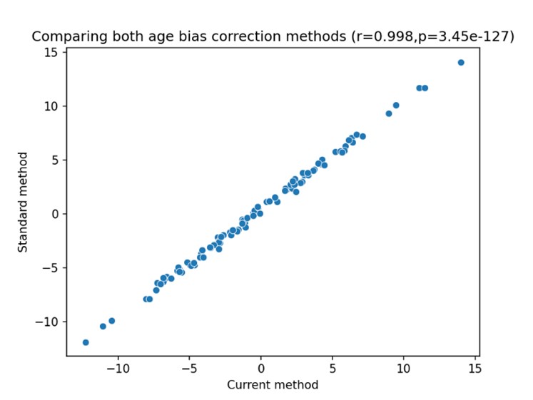
The x-axis represents the first method, used in the current study, and the y-axis represents the second method, described in Smith et al., (2019). Across all subjects, we found a nearly perfect 1:1 correspondence between the two methods (r=.998, p<0.001; MAE=0.45), as the two are mathematically identical. The small gap between the two is because the brain age attenuation model also takes into account the difference in the exact time that passed between the two scans for each participant (mean=21.36m, std = 1.68m).
We now note this in Methods section 4.9:
“We note that the result of computing the difference between the bias-corrected brain age gap at both times was nearly identical to the brain age attenuation measure (r=.99, p<0.001; MAE=0.45). The difference between the two is because the brain age attenuation model takes into account the difference in the exact time that passed between the two scans for each participant (mean=21.36m, std = 1.68m).”
3) In Figure 3, some of the changes observed between time points are very large. For example, one subject with a chronological age of 62 shows a ten-year increase in brain age over 18 months. This change is twice as large as the full range of age variation in the brain age estimates (average brain age increases from 50 to 55 across the full chronological age span). This makes it difficult to interpret RSFC change in units of brain age. E.g., is it reasonable that a person's brain ages by ten years, either up or down, in 18 months? The colour scale goes from -12 years to 14 years, so some of the observed changes are 14 / 1.5 = 9 times larger than the actual time from baseline to follow-up.
- The questions above should be investigated and addressed in the context of potential challenges with using brain age as a marker (see e.g., https://onlinelibrary.wiley.com/doi/full/10.1002/hbm.25837, https://onlinelibrary.wiley.com/doi/full/10.1002/hbm.26144).
We agree that our model precision was relatively low, especially compared to the period of the intervention, as also stated by reviewer #1. We now discuss this issue in light of the studies pointed out by the reviewer (Discussion section):
“In the current work, we used RSFC for brain age estimation, which resulted in a MAE of ~8 years, which was larger than the intervention period. Nevertheless, we found that brain age attenuation was associated with changes in multiple health factors. The precision of an age prediction model based on RSFC is typically lower than a model based on structural brain imaging5. However, a higher model precision may result in a lower sensitivity to detect clinical effects6,7. Better tools for data harmonization among datasets6 and larger training sample size5 may improve the accuracy of such models in the future.”
Again, we note that despite the moderate precision accuracy, we replicated these results in three separate cohorts and found that both the correlation and the MAE between the predicted and observed age were significant in all of them.
RSFC for age prediction:
1) Several studies show better age prediction accuracy with structural MRI features compared to RSFC. If the focus of the study is to use an accurate estimate of brain ageing rather than specifically looking at changes in RSFC, adding structural MRI data could be helpful.
We focused on brain structural changes in a previous work, and the focus of the current work was assessing age-related functional connectivity alterations. We now added a few sentences in the Introduction section that would hopefully better motivate our choice:
“We previously found that weight loss, glycemic control, lowering of blood pressure, and increment in polyphenols-rich food were associated with an attenuation in brain atrophy 12. Obesity is also manifested in age-related changes in the brain’s functional organization as assessed with resting-state functional connectivity (RSFC). These changes are dynamic13 and can be observed in short time scales14 and thus of relevance when studying lifestyle intervention.”
2) If changes in RSFC are the main focus, using brain age adds a complicated layer that is not necessarily helpful. It could be easier to simply assess RSFC change from baseline to follow up, and correlate potential changes with changes in e.g., BMI.
We are specifically interested in age-related changes as we described a-priori in the registration of the study: https://clinicaltrials.gov/ct2/show/NCT03020186
Moreover, age-related changes in RSFC are complex, multivariate and dependent upon the choice of theoretical network measures. We think that a data-driven brain age prediction approach might better capture these multifaceted changes and their relation to aging. We now state this in the Introduction section:
“Studies have linked obesity with decreased connectivity within the default mode network15,16 and increased connectivity with the lateral orbitofrontal cortex17, which are also seen in normal aging18,19. Longitudinal trials have reported changes in these connectivity patterns following weight reduction20,21, indicating that they can be altered. However, findings regarding functional changes are less consistent than those related to anatomical changes due to the multiple measures22 and scales23 used to quantify RSFC. Hence, focusing on a single measure, the functional brain age, may better capture these complex, multivariant changes and their relation to aging. “
The lack of control groups
1) If no control group data is available, it is important to clarify this in the manuscript, and evaluate which conclusions can and cannot be drawn based on the data and study design.
We agree that this point should be made more clear, and we now state this in the limitation section of the Discussion:
“We also note that the lack of a no-intervention control group limits our ability to directly relate our findings to the intervention. Hence, we can only relate brain age attenuation to the observed changes in health biomarkers.”
Also, following reviewers’ #2 and #3 comments, we refer to the weight loss following 18 months of lifestyle intervention instead of to the intervention itself. This is now made clear in the title, abstract, and the main text.
Reviewer #3 (Public Review):
The authors report on an interesting study that addresses the effects of a physical and dietary intervention on accelerated/decelerated brain ageing in obese individuals. More specifically, the authors examined potential associations between reductions in Body-Mass-Index (BMI) and a decrease in relative brain-predicted age after an 18-months period in N = 102 individuals. Brain age models were based on resting-state functional connectivity data. In addition to change in BMI, the authors also tested for associations between change in relative brain age and change in waist circumference, six liver markers, three glycemic markers, four lipid markers, and four MRI fat deposition measures. Moreover, change in self-reported consumption of food, stratified by categories such as 'processed food' and 'sweets and beverages', was tested for an association with change in relative brain age. Their analysis revealed no evidence for a general reduction in relative brain age in the tested sample. However, changes in BMI, as well as changes in several liver, glycemic, lipid, and fat-deposition markers showed significant covariation with changes in relative brain age. Three markers remained significant after additionally controlling for BMI, indicating an incremental contribution of these markers to change in relative brain age. Further associations were found for variables of subjective food consumption. The authors conclude that lifestyle interventions may have beneficial effects on brain aging.
Overall, the writing is concise and straightforward, and the langue and style are appropriate. A strength of the study is the longitudinal design that allows for addressing individual accelerations or decelerations in brain aging. Research on biological aging parameters has often been limited to cross-sectional analyses so inferences about intra-individual variation have frequently been drawn from inter-individual variation. The presented study allows, in fact, investigating within-person differences. Moreover, I very much appreciate that the authors seek to publish their code and materials online, although the respective GitHub project page did not appear to be set to 'public' at the time (error 404). Another strength of the study is that brain age models have been trained and validated in external samples. One further strength of this study is that it is based on a registered trial, which allows for the evaluation of the aims and motivation of the investigators and provides further insights into the primary and secondary outcomes measures (see the clinical trial identification code).
One weakness of the study is that no comparison between the active control group and the two experimental groups has been carried out, which would have enabled causal inferences on the potential effects of different types of interventions on changes in relative brain age. In this regard, it should also be noted that all groups underwent a lifestyle intervention. Hence, from an experimenter's perspective, it is problematic to conclude that lifestyle interventions may modulate brain age, given the lack of a control group without lifestyle intervention. This issue is fueled by the study title, which suggests a strong focus on the effects of lifestyle intervention. Technically, however, this study rather constitutes an investigation of the effects of successful weight loss/body fat reduction on brain age among participants who have taken part in a lifestyle intervention. In keeping with this, the provided information on the main effect of time on brain age is scarce, essentially limited to a sign test comparing the proportions of participants with an increase vs. decrease in relative brain age. Interestingly, this analysis did not suggest that the proportion of participants who benefit from the intervention (regarding brain age) significantly exceeds the number of participants who do not benefit. So strictly speaking, the data rather indicates that it's not the lifestyle intervention per sé that contributes to changes in brain age, but successful weight loss/body fat reduction. In sum, I feel that the authors' claims on the effects of the intervention cannot be underscored very well given the lack of a control group without lifestyle intervention.
We agree that this point, also raised by reviewer #2, should be made clear, and we now state this in the limitation section of the Discussion:
“We also note that the lack of a no-intervention control group limits our ability to directly relate our findings to the intervention. Hence, we can only relate brain age attenuation to the observed changes in health biomarkers.”
Also, following reviewers #2 and #3, we refer to the weight loss following 18 months of lifestyle intervention instead of to the intervention itself. This is now explicitly mentioned in the title, abstract, and within the text:
Title: “The effect of weight loss following 18 months of lifestyle intervention on brain age assessed with resting-state functional connectivity”
Abstract: “…, we tested the effect of weight loss following 18 months of lifestyle intervention on predicted brain age, based on MRI-assessed resting-state functional connectivity (RSFC).”
Another major weakness is that no rationale is provided for why the authors use functional connectivity data instead of structural scans for their age estimation models. This gets even more evident in view of the relatively low prediction accuracies achieved in both the validation and test sets. My notion of the literature is that the vast majority of studies in this field implicate brain age models that were trained on structural MRI data, and these models have achieved way higher prediction accuracies. Along with the missing rationale, I feel that the low model performances require some more elaboration in the discussion section. To be clear, low prediction accuracies may be seen as a study result and, as such, they should not be considered as a quality criterion of the study. Nevertheless, the choice of functional MRI data and the relevance of the achieved model performances for subsequent association analysis needs to be addressed more thoroughly.
We agree that age estimation from structural compared to functional imaging yields a higher prediction accuracy. In a previous publication using the same dataset12, we demonstrated that weight loss was associated with an attenuation in brain atrophy, as we describe in the introduction:
“We previously found that weight loss, glycemic control and lowering of blood pressure, as well as increment in polyphenols rich food, were associated with an attenuation in brain atrophy 12.”
Here we were specifically interested in age-related functional alterations that are associated with successful weight reduction. Compared to structural brain changes aging effect on functional connectivity is more complex and multifaced. Hence, we decided to utilize a data-driven or prediction-driven approach for assessing age-related changes in functional connectivity by predicting participants’ functional brain age. We now describe this rationale in the introduction section:
“Studies have linked obesity with decreased connectivity within the default mode network15,16 and increased connectivity with the lateral orbitofrontal cortex17, which are also seen in normal aging18,19. Longitudinal trials have reported changes in these connectivity patterns following weight reduction20,21, indicating that they can be altered. However, findings regarding functional changes are less consistent than those related to anatomical changes due to the multiple measures22 and scales23 used to quantify RSFC. Hence, focusing on a single measure, the functional brain age, may better capture these complex changes and their relation to aging.”
We address the point regarding the low model performance in response to reviewer #2, comment #2.
Author Response:
Evaluation Summary:
The authors studied the neural correlates of planning and execution of single finger presses in a 7T fMRI study focusing on primary somatosensory (S1) and motor (M1) cortices. BOLD patterns of activation/deactivation and finger-specific pattern discriminability indicate that M1 and S1 are involved not only during execution, but also during planning of single finger presses. These results contribute to a developing story that the role of primary somatosensory cortex goes beyond pure processing of tactile information and will be of interest for researchers in the field of motor control and of systems neuroscience.
We thank all reviewers and the editor for their assessment of our paper. We acknowledge that our description of the methods and some interpretation of the results can be clarified and expanded. We address every comment and proposed suggestion in the following below.
Reviewer #1 (Public Review):
This is a very important study for the field, as the involvement of S1 in motor planning has never been described. The paradigm is very elegant, the methods are rigorous and the manuscript is clearly written. However, there are some concerns about the interpretation of the data that could be addressed.
We thank Reviewer #1 for the positive evaluation of our study. We clarify our methodological choices and interpretation of the data in the following response.
• The authors claim that planning and execution patterns are scaled version of each other, and that overt movement during planning is prevented by global deactivation. This is an interesting perspective, however the presented data are not fully convincing to support this claim:
(1) the PCM analysis shows that correlation models ranging from 0.4 to 1 perform similarly to the best correlation model. This correlation range is wide and suggests that the correspondence between execution/planning patterns is only partial.
The reviewer is correct that the current data leaves us with a specific amount of uncertainty. However, it should be noted that the maximum-likelihood estimates of correlations between noisy patterns are biased, as they are constrained to be smaller or equal to 1. Thus, we cannot test the hypothesis that the correlation is 1 by just comparing correlation estimates to 1 (for details on this, see our recent blog on this topic: http://www.diedrichsenlab.org/BrainDataScience/noisy_correlation/). To test this idea, we therefore use a generative approach (the PCM analysis). We find that no correlation model has a higher log-likelihood than the 1-correlation model, therefore we cannot rule out that the underlying true correlation is actually 1. In other words, we have as much evidence that the correspondence is only partial as we do that the correspondence is perfect. The ambiguity given by the wide correlation range is due to the role of measurement noise in the data and should not be interpreted as if the true correlation was lower than 1. What we can confidently conclude is that activity patterns have a substantial positive correlation between planning and execution. We take this opportunity to clarify this point in the results section.
(2) in Fig.4 A-B, the distance between execution/planning patterns is much larger than the distance between fingers. How can such a big difference be explained if planning/execution correspond to scaled versions of the same finger-specific patterns? If the scaling is causing this difference, then different normalization steps of the patterns should have very specific effects on the observed results: 1) removing the mean value for each voxel (separately for execution and planning conditions) should nullify the scaling and the planning/execution patterns should perfectly align in a finger-specific way; 2) removing the mean pattern (separately for each finger conditions) should effectively disturb the finger-specific alignment shown in Fig.4C. These analyses would corroborate the authors' conclusion.
The large distance between planning and execution patterns (compared to the distance between fingers) is caused by the fact that the average activity pattern associated with planning differs substantially from the average activity pattern during execution. Such a large difference is of course expected, given the substantially higher activity during execution. However, here we are testing the hypothesis that the pattern vectors that are related to a specific finger within either planning or execution are scaled version of each other. Visually, this can be seen in Figure 4B (bottom), where the MDS plot is rotated, such the line of sight is in the direction of the mean pattern difference between planning and execution—such that it disappears in the projection. Relative to the baseline mean of the data (cross), you can see that arrangement of the fingers in planning (orange) is a scaled version of the arrangement during execution (blue). The PCM model provides a likelihood-based test for this idea. The model accounts for the overall difference between planning and execution by including (and estimating) model terms related to the mean pattern of planning and execution, respectively, therefore effectively removing the mean activation of planning and execution. We have now explained this better in the results and methods sections, also referring to a Jupyter notebook example of the correlation model used (https://pcm-toolbox-python.readthedocs.io/en/latest/demos/demo_correlation.html).
Regarding your analysis suggestions, removing the mean pattern for planning and execution across fingers as a fixed effect (suggestion 1) leads to the distance structure shown in Fig 4B (bottom)—showing that the finger-specific patterns during planning are scaled versions of those during execution (also see Fig. R1 below). On the other hand, subtracting the mean finger pattern across planning and execution (suggestion 2) will not fully remove the finger specific activation as the finger-specific patterns are differently scaled in planning and execution. Furthermore, neither of these subtraction analyses allows for a formal test of the hypotheses that the data can be explained by a pure scaling of the finger-specific patterns.
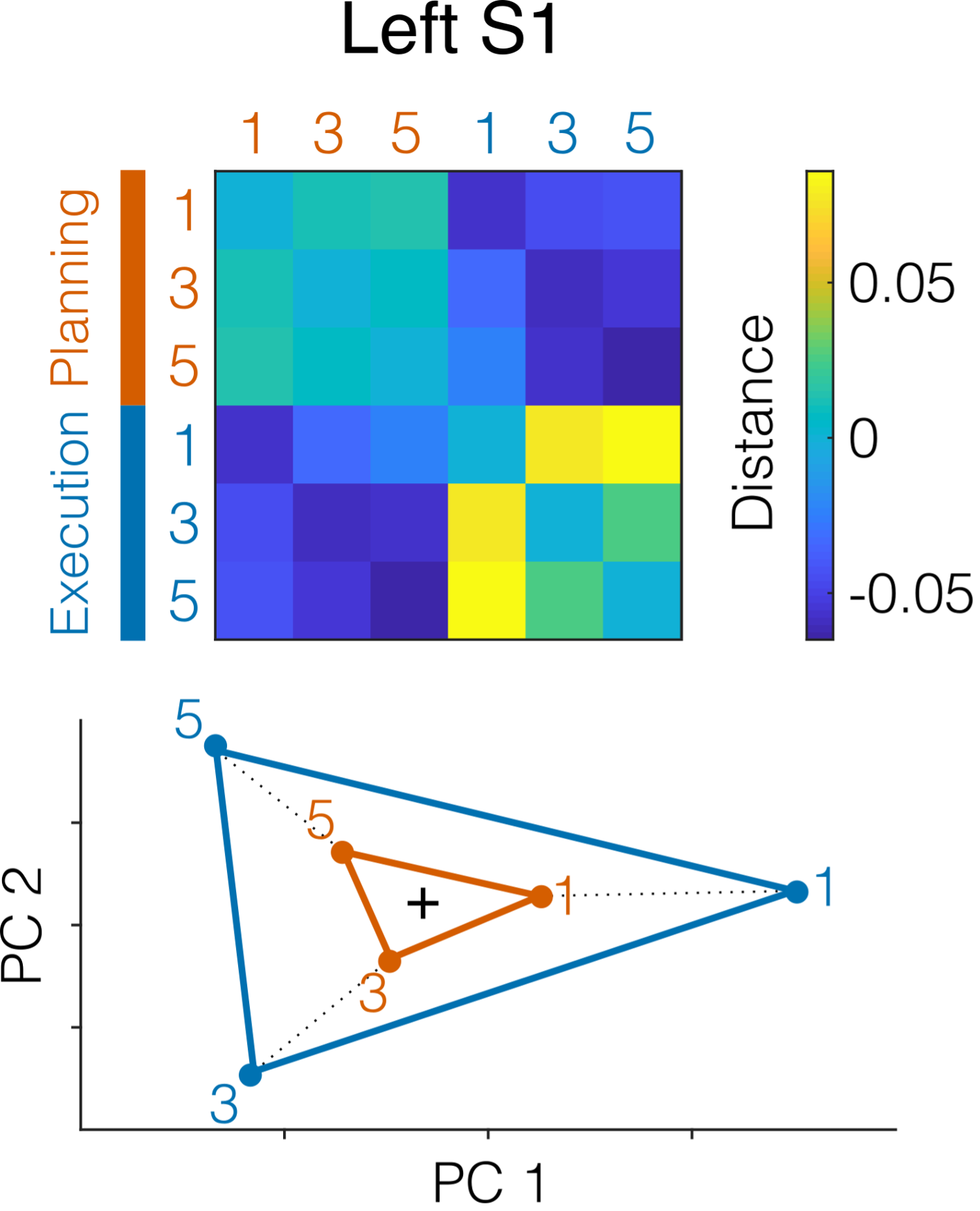
Figure R1. RDM of left S1 activity patterns evoked by the three fingers (1, 3, 5) during no-go planning (orange) and execution (blue) after removing the mean pattern across fingers (separately for planning and execution). The bottom shows the corresponding multidimensional scaling (MDS) projection of the first two principal components. Black cross denotes mean pattern across conditions.
• A conceptual concern is related to the task used by the authors. During the planning phase, as a baseline task, participants are asked to maintain a low and constant force for all the fingers. This condition is not trivial and can even be considered a motor task itself. Therefore, the planning/execution of the baseline task might interfere with the planning/execution of the finger press task. Even more controversial, the design of the motor task might be capturing transitions between different motor tasks (force on all finger towards single-finger press) rather than pure planning/execution of a single task. The authors claim that the baseline task was used to control for involuntary movements, however, EMG recordings could have similarly controlled for this aspect, without any confounds.
Participants received training the day before scanning, which made the “additional” motor task very easy, almost trivial. In fact, the system was calibrated so that the natural weight of the hand on the keys was enough to bring the finger forces within the correct range to be maintained. Thus, very little planning/online control was required by the participants before pressing the keys. As for the concern of capturing transitions between different motor tasks, that it is indeed always the case in natural behavior. Arguably there is no such thing as “pure rest” in the motor system, active effort has to be made even to maintain posture. Furthermore, if the motor system considers the hold phase as a simultaneous movement phase, it should have prevented M1 and S1 to participate in the planning of upcoming movements, as it would be busy with maintaining and controlling the pre-activation. Having found clear planning related signals in M1 and S1 in this situation makes our argument, if anything, stronger.
Finally, we specifically chose not to do EMG recordings because finger forces are a more sensitive measure of micro movements than EMG. Extensive pilot experiments for our papers studying ipsilateral representations and mirroring (e.g., Diedrichsen et al., 2012; Ejaz et al., 2018) have shown that we can pick up very subtle activations of hand muscles by measuring forces of a pre-activated hand, signals that clearly escape detection when recording EMG in the relaxed state. Based on these results, we actually consider the recording of EMG during the relaxed state as an insufficient control for the absence of cortical-spinal drive onto hand muscles. This is especially a concern when recording EMG during scanning, due to the decreased signal-to-noise ratio.
• In Fig.2F, the authors show no-planning related information in high-order areas (PMd, aSPL), while such information is found in M1 and S1. This null result from premotor and parietal areas is rather surprising, considering current literature, largely cited by the authors, pointing to high-order motor or parietal areas involved in action planning.
We agree with the reviewer that, to some extent, the lack of involvement of high-order areas in planning is surprising. However, we believe that task difficulty (i.e., planning demands) plays a role in the amount of observed planning activation. In other words, because participants were only asked to plan repeated movements of one finger, there was little to plan. The fact that this may have contributed to the null result in premotor and parietal areas was further confirmed by the second half of the dataset, which is not reported in the current paper. Here, we investigated the planning of multi-finger sequences, where planning demands are certainly higher. We found that high-order areas such as PMd and SPL were indeed active and involved in the planning of those, as expected. We decided to split the dataset across two publications as the multi-finger sequences have their own complexities, which would have distracted from the main finding of planning related activity in M1 and S1.
Reviewer #3 (Public Review):
I found the manuscript to be well written and the study very interesting. There are, however, some analytical concerns that in part arise because of a lack of clarity in describing the analyses.
1) Some details regarding the methods used and results in the figures were missing or difficult to understand based on the brief description in the Methods section or figure legend.
We thank Reviewer #3 for pointing out some lack of clarity in our description of the methods. We now expanded both the methods section and the figure captions (Fig. 2-3-4).
2) I think the manuscript would benefit from a more balanced description on the role of S1. As the authors state, S1 is traditionally thought to process afferent tactile and proprioceptive input. However, in the past years, S1 has been shown to be somatopically activated during touch observation, attempted movements in the absence of afferent tactile inputs, and through attentional shifts (Kikkert et al., 2021; Kuehn et al., 2014; Puckett et al., 2017; Wesselink et al., 2019). Furthermore, S1 is heavily interconnected with M1, so perhaps if such activity patterns are present in M1, they could also be expected in S1?
To better characterize the role of S1 during movement planning, we now include recent research showing that S1 can be somatotopically recruited even in the absence of tactile inputs.
3) Related to the previous comment: If attentional shifts on fingers can activate S1 somatotopically, could this potentially explain the results? Perhaps the participants were attending to the fingers that were cued to be moved and this would have led to the observed activity patterns. I don't think the data of the current study allows the authors to tease apart these potential contributions. It is likely that both processes contribute simultaneously.
We agree that our results could also be explained by attentional shifts on the fingers. It is very likely that, during planning, participants were specifically focusing on the cued finger. However, as the reviewer points out, our current dataset cannot distinguish between planning and attention as voluntary planning requires attention. We expanded the discussion section to include this possibility.
4) The authors repeatedly interpret the absences of significant differences as indicating that the tested entities are the same. This cannot be concluded based on results of frequentist statistical testing. If the authors would like to make such claims, then they I think they should include Bayesian analysis to investigate the level of support for the null hypothesis.
We have now clarified the parts in the manuscript that sounded as if we were interpreting the absence of significant difference (null results) as significant absence of differences (equivalence).
Author Response
Reviewer #1 (Public Review):
This study investigates how pathogens might shape animal societies by driving the evolution of different social movement rules. The authors find that higher disease costs induce shifts away from positive social movement (preference to move towards others) to negative social movement (avoidance from others). This then has repercussions on social structure and pathogen spread.
Overall, the study comprises a good mixture of intuitive and less intuitive results. One major weakness of the work, however, is that the model is constructed around one pathogen that repeatedly enters a population across hundreds of generations. While the authors provide some justification for this, it does not capture any biological realism in terms of the evolution of the pathogen itself, which would be expected. The lack of co-evolution in the model substantially limits the generality of the results. For example, a number of recent studies have reported that animals might be expected to become very social when pathogens are very infectious, because if the pathogen is unavoidable they may as well gain the benefits of being social. The authors make some arguments about being focused on introduction events, but this does not really align well with their study design that carries through many generations after the introduction. Given the rapid evolutionary dynamics, perhaps the study could have a more focused period immediately after the initial introduction of the pathogen to look at rapid evolutionary responses (albeit this may need some sensitivity analyses around the parameters such as the mutation rates).
We appreciate the reviewer’s evaluation of our work, and acknowledge that we have not currently included evolutionary dynamics for the pathogen.
One conceptual impediment to such inclusion is knowing how pathogen traits could be modelled in a mechanistic way. For example, it is widely held that there is a trade-off between infection cost and transmissibility, with a quadratic relationship between them, but this is a pattern and not a process per se. We are unsure which mechanisms could be modelled that impinge upon both infection cost and transmissibility.
On the practical side, we feel that a mechanistic, individual-based model that includes both pathogen and host evolution would become very challenging to interpret. It might be more tractable to begin with a mechanistic, spatial model that examines pathogen trait evolution with an unchanging host (such as an adaptation of Lion and Boots, 2010). We would be happy to take this on in future work, with a view to combining models thereafter.
We have taken the suggestion to focus on the period immediately after the introduction, and we now focus on the following 500 generations. While 500 generations is still a long time, we would note that our model dynamics typically stabilise within 200 generations. We show the following generations primarily to check that some stability in the dynamics has indeed been reached (but see our new scenario 2).
We also appreciate the point regarding mutation rates. Our mutation rates are relatively high to account for the small size of our population. We have found that with smaller mutation rates (0.001 rather than 0.01), evolutionary shifts in our population do not occur within the first 500 generations. This is primarily because prior to pathogen introduction, the ‘agent avoiding’ strategy that becomes common later is actually quite rare. Whether a rapid transition takes place thus depends on whether there are any agent avoiding individuals in the population at the moment of pathogen introduction, or on whether such individuals emerge rapidly thereafter through mutations on the social weights. We expect that with larger population sizes, we would be able to recover our results with smaller mutation rates as well.
A final, and much more minor comment is whether this is really a paper about movement. The model does not really look at evolutionary changes in how animals move, but rather at where they move. How important is the actual movement process under this model? For example, would the results change if the model was constructed without explicit consideration of space and resources, but instead simply modelled individuals' decisions to form and break ties? (Similar to the recent paper by Ashby & Farine https://onlinelibrary.wiley.com/doi/full/10.1111/evo.14491 ). It might help to provide more information about how putting social decisions into a spatially explicit framework is expected to extend studies that have not done so (e.g.., because they are analytical).
This paper is indeed about movement, as where to move is a key part of the movement ecology paradigm (Nathan et al. 2008). That said, we appreciate the advice to emphasise the importance of social decisions in a spatial context, we have added these to the Introduction (L. 79 – 81) and Discussion (L. 559 – 562). In brief, we do expect different dynamics that result from the explicit spatial context, as compared to a model in which social associations are probabilistic and could occur with any individual in the population.
In our models, individual social tendency (whether they are prefer moving towards others) is separated from individual sociality (whether they actually associate with other individuals). This can be seen from our (new) Fig. 3D, in which individuals of each of the social strategies can sometimes have similar numbers of associations (although modulated by movement). This separation of the pattern from the underlying process is possible, we believe, due to the heterogeneity in the social landscape created by the explicit spatial context.
Reviewer #2 (Public Review):
This theoretical study looks at individuals' strategies to acquire information before and after the introduction of pathogens into the system. The manuscript is well-written and gives a good summary of the previous literature. I enjoyed reading it and the authors present several interesting findings about the development of social movement strategies. The authors successfully present a model to look at the costs and benefits of sociality.
I have a couple of major comments about the work in its current form that I think are very important for the authors to address. That said, I think this is a promising start and that with some revisions, this could be a valuable contribution to the literature on behavioral ecology.
We appreciate the reviewer’s kind words.
Before starting, I would like to be precise that, given the scope of the models and the number of parameter choices that were necessary, I am going to avoid criticisms of the decisions made when designing the models. However, there are a few assumptions I rather find problematic and would like to give proper attention to.
The first regards social vs. personal information. Most of the model argumentation is based on the reliance on social information (considering four, but to me overlapping, social strategies that are somehow static and heritable) but in fact, individuals may oscillate between relying on their personal information and/or on social information -- which may depend on the availability of resources, population density, stochastic factors, among others (Dall et al. 2005 Trends Ecol. Evol., Duboscq et al. 2016 Frontiers in Psychology). In my opinion, ignoring the influence of personal and social information decreases the significance of this work. I am aware that the authors consider the detection of food present in the model, but this is considered to a much smaller extent (as seen in their weight on individual decisions) than the social information cues.
We appreciate the point that individuals can switch between relying on social and personal information. However, we would point out that in our model, the social strategies are not static. The social strategy is a convenient way of representing individuals’ position in behavioural trait-space (the ‘behavioural hypervolume’ of Bastille-Rousseau and Wittemeyer 2019). This essentially means that the importance assigned to each of the three cues available in our model varies among individuals. There are indeed individuals that are primarily guided by the density of food items, and this is the commonest ‘overall’ movement strategy before the pathogen is introduced. We represent this by showing how the importance of social information is low before pathogen introduction (Fig. 2B).
While we primarily focus on the importance of social information, this is because the population quite understandably evolves a persistent preference for moving towards food items (i.e., using personal information if available). We have made this clearer in the text on lines 367 – 371.
Critically, it is also unclear how, if at all, the information and pathogen traits are related to each other. If a handler gets sick, how does this affect its foraging activity (does it stop foraging, slow its activities, or does it show signs of sickness)? Perhaps this model is attempting to explore the emergence of social movement strategies only, but how they disentangle an individual's sickness status and behavioral response is unclear.
We appreciate that infection may lead to physiological effects (e.g. altered metabolic rates, reduction in cognitive capacity) that may then influence behaviour. Our model aims to be relatively simple and general one, and does not consider the explicit mechanisms by which infection imposes a cost on fitness. Thus we do not include any behavioural modifications due to infection, as we feel that these would be much too complex to include in such a model. We would be happy to explore, in future work, phenomena such as the evolution of self-isolation and infection detection which is common among animals such as social insects (Stroeymeyt et al. 2018, Pusceddu et al. 2021).
However, we have considered an alternative implementation of our model’s scenario 1 which could be interpreted as the infection reducing foraging efficiency by a certain percentage (other interpretations of the redirection of energy away from reproduction are also possible). We show how this implementation leads to very similar outcomes as those seen in our
Very little is presented about the virulence of the pathogens and how they could affect the emergence of social strategies. The authors keep their main argumentation based on the introduction of novel pathogens (without distinctions on their pathogenicity), but a behavioral response is rather influenced by how fast individuals are infected and which are their chances of recovering. Besides, they consider that only one or two social interactions would be enough for pathogen transmission to occur.
We have indeed considered a fixed transmission probability of 0.05, a relatively modest attack rate. Setting transmission probability to two other values (0.025, 0.1), we find that our general results are recovered - there is an evolutionary transition away from sociality, with the proportion of agent avoidance evolved increasing with the transmission probability. While we do not show these results in the main text, we have included figures showing the proportions of each social movement strategy here for the reviewers’ reference.
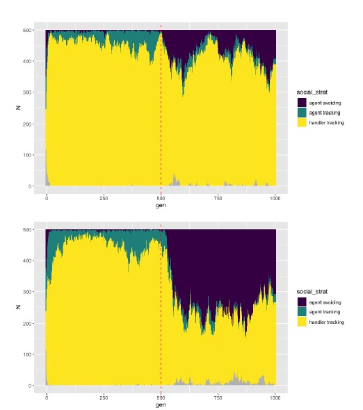
Figures showing the proportion of social movement strategies in two simulation runs of our default implementation of scenario 1 (dE = 0.25, R = 2, pathogen introduction begins from G = 500). Top: Probability of transmission = 0.025 (half of the default). Bottom: Probability of transmission = 0.10 (double the default). Overall, the proportion of agent avoidance evolved (purple) increases with the probability of transmission. Each figure shows a single replicate of each parameter combination, for only 1,000 generations.
Another important component is that individuals do not die, and it seems that they always have a chance (even if it is small) to reproduce. So, how the authors consider unsuccessful strategies in the model outputs or how these social strategies would be potentially "dismissed" by natural selection are not considered.
We appreciate the point that our simulation does not include mortality effects, and that all individuals have some small chance of reproducing. There are a few practical and conceptual challenges when incorporating this level of realism in a general model. Including mortality effects could allow for the emergence of more complex density-dependent dynamics, as dead individuals would not be able to transmit the pathogen to other foragers (although for some pathogens, this could be a valid choice), nor would they be sources of social information. This would make the model much more challenging to interpret, and we have tried to keep this model as simple as possible.
We have also sought to keep the model’s focus on the evolutionary dynamics, and to not focus on mortality. In order to balance this aim with the reviewer's suggestion, we have included a new implementation of the model’s scenario 1 which has a threshold on reproduction. That means that only individuals with a positive energy balance (intake > infection costs) are allowed to reproduce. We show a potentially counter-intuitive result, that the more social ‘handler tracking’ strategy persists at a higher frequency than in our default implementation, despite having a higher infection rate than the ‘agent avoiding’ strategy. We suggest that this is because the ‘agent avoiding’ individuals have very low or no intake. This is sufficient in our default implementation to have relatively higher fitness than the more frequently infected handler tracking individuals.
Reviewer #3 (Public Review):
Gupte and colleagues develop an individual-based model to examine how the introduction of a novel pathogen influences the evolution of social cue use in a population of agents for which social cues can both facilitate more efficient foraging, but also expose individuals to infection. In their simulations, individuals move across a landscape in search of food, and their movements are guided by a combination of cues related to food patches, individuals that are currently handling food items, and individuals that are not actively handling food. The latter two cues can provide indirect information about the likely presence of food due to the patchiness of food across the landscape.
The authors find that prior to introducing the novel pathogen, selection favors strategies that home in on agents, regardless of whether those agents are currently handling food items. The overall contribution of these social cues to movement decisions, however, tends to be relatively small. After pathogen introduction, agents evolve to rely more heavily on social information and to either be more selective in their use of it (attending to other agents that are currently handling food and avoiding non-handlers) or avoiding other agents altogether. Gupte and colleagues further examine the ecological consequences of these shifts in social decision-making in terms of individuals' overall movement, food consumption, and infection risk. Relative to pre-introduction conditions, individuals move more, consume less food, and are less likely to be infected due to reduced contact with others. Epidemiological models on emergent social networks confirm that evolved behavioral changes generate networks that impede the spread of disease.
The introduction of novel pathogens into wild populations is expected to be increasingly common due to climate change and increasing global connectedness. The approach taken here by the authors is a potentially worthwhile avenue to explore the potential eco-evolutionary consequences of such introductions. A major strength of this study is how it couples ecological and evolutionary timescales. Dominant behavioral strategies evolve over time in response to changing environmental conditions and impact social, foraging, and epidemiological dynamics within generations. I imagine there are many further questions that could be fruitfully explored using the authors' framework. There are, however, important caveats that impact the interpretation of the authors' findings.
First, reproduction bears no cost in this model. Individuals produce offspring in proportion to their lifetime net energy intake, which is increased by consuming food and decreased by a set amount per turn once infected. However, prior to reproduction, net energy intake is normalized (0-1) according to the lowest individual value within the generation. This means that individuals need not maintain a positive energy balance nor even consume food at all to successfully reproduce, so long as they perform reasonably well relative to other members of the population. Since consuming food is not necessary to reproduce, declining per capita intake due to evolved social avoidance (Fig. 1d) likely decreases the importance of food to an individual's reproductive success relative to simply avoiding infection. This dynamic could explain the delayed emergence of the 'agent avoiding' strategy (Fig. 1a), as this strategy potentially is only viable once per capita intake reaches a sufficiently low level across the population (Fig. 1d). I am curious to know what the results would be if reproduction required some minimal positive net energy, such that individuals must risk food patches in order to reproduce. It would also be useful for the authors to provide information on how net energy intake changes across generations, as well as whether (and if so, how) attraction to the food itself may change over time.
We thank the reviewer for their assessment of our work, and appreciate the point raised here (and in an earlier review) about individuals potentially reproducing without any intake. We have addressed this by running our default model [repeated introductions, R = 2, dE = 0.25], with a threshold on reproduction such that only individuals with a positive energy balance can reproduce. We mention these results in the text (L. 495 – 500), and show related figures in the SI Appendix. In brief, as the reviewer suggests, agent avoiding is less common for our default parameter combination, but becomes as common as the default combination when the infection cost is doubled (to dE = 0.5).
We appreciate the reviewer’s suggestion about decreasing per-capita intake being a precondition for the proliferation of the agent avoiding strategy. With our new results, we now show that there is no overall decrease in intake, but the agent avoiding strategy still becomes a common strategy after pathogen introduction. As the reviewer suggests, this is because these individuals have an equivalent net energy as handler tracking individuals, as they are less frequently infected.
We suggest that the delayed emergence of the agent avoiding strategy is primarily due to mutation limitations – such individuals are uncommon or non-existent in the simulation before pathogen introduction, and random mutations are required for them to emerge. As we have noted in response to an earlier comment, this becomes clear when the mutation rate is reduced from 0.01 to 0.001 – agent avoidance usually does not evolve at all.
A second important caveat is that the evolutionary responses observed in the model only appear when novel pathogen introductions are extremely frequent. The model assumes no pathogen co-evolution, but rather that the same (or a functionally identical) pathogen is re-introduced every generation (spillover rate = 1.0). When the authors considered whether evolutionary responses were robust to less frequent introductions, however, they found that even with a per-generation spillover rate of 0.5, there was no impact on social movement strategies. The authors do discuss this caveat, but it is worth highlighting here as it bears on how general the study's conclusions may be.
We appreciate the reviewer’s point entirely. We would point out that current knowledge about pathogen introductions across species and populations in the wild is very poor. However, the ongoing highly pathogenic avian influenza outbreak (Wille and Barr 2022), the spread of multiple strains of SARS-CoV-2 to wild deer in several different human-to-wildlife transmission events, and recent work on the potential for coronavirus spillovers from bats to humans, all suggest that at least some generalist pathogens must circulate quite widely among wildlife, often crossing into novel host species or populations. We have added these considerations to the text on lines 218 – 231.
We have also added, in order to confront this point more squarely, a new scenario of our model in which the pathogen is introduced just once, and then transmits vertically and horizontally among individuals (lines 519 – 557). This scenario more clearly suggests when evolutionary responses to pathogen introductions are likely to occur, and what their consequences might be for a pathogen becoming endemic in a population. This scenario also serves as a potential starting point for models of host-pathogen trait co-evolution, and we have added this consideration to the text on lines 613 – 623.
References
● Albery, G. F. et al. 2021. Multiple spatial behaviours govern social network positions in a wild ungulate. - Ecology Letters 24: 676–686.
● Bastille-Rousseau, G. and Wittemyer, G. 2019. Leveraging multidimensional heterogeneity in resource selection to define movement tactics of animals. - Ecology Letters 22: 1417–1427.
● Gupte, P. R. et al. 2021. The joint evolution of animal movement and competition strategies. - bioRxiv in press.
● Lion, S. and Boots, M. 2010. Are parasites ‘“prudent”’ in space? - Ecology Letters 13: 1245–1255.
● Lloyd-Smith, J. O. et al. 2005. Superspreading and the effect of individual variation on disease emergence. - Nature 438: 355–359.
● Nathan, R. et al. 2008. A movement ecology paradigm for unifying organismal movement research. - PNAS 105: 19052–19059.
● Pusceddu, M. et al. 2021. Honey bees increase social distancing when facing the ectoparasite varroa destructor. - Science Advances 7: eabj1398.
● Sánchez, C. A. et al. 2022. A strategy to assess spillover risk of bat SARS-related coronaviruses in Southeast Asia. - Nat Commun 13: 4380.
● Stroeymeyt, N. et al. 2018. Social network plasticity decreases disease transmission in a eusocial insect. - Science 362: 941–945.
● Wilber, M. Q. et al. 2022. A model for leveraging animal movement to understand spatio-temporal disease dynamics. - Ecology Letters in press.
● Wille, M. and Barr, I. G. 2022. Resurgence of avian influenza virus. - Science 376: 459–460.
Author Response:
Reviewer #1:
In the manuscript by Kymre, Liu and colleagues, the authors investigate how pheromone signals are interpreted by the projection neurons of the male moth brain. While the olfactory neurons and glomerular targets of pheromone signaling is known, the signaling of the projection neurons (output neurons) that carry pheromone signaling to higher regions of the brain remained unknown. The authors utilized a series of technically challenging experiments to identify the anatomy and functional responses of projection neurons responding to pheromone mixtures, primary pheromone, secondary pheromone, and behavioral antagonist odors. By calcium imaging of MGC mALT neurons, the authors identify that odor responses in PNs are broader than the olfactory neuron counterparts (ie, the behavioral antagonist activates OSNs innervating the dma glomerulus, whereas the antagonist actives dma and dmp glomeruli). The authors then perform a series of elegant experiments by which the odor responses of different mALT PNs are recorded by electrophysiology, and the anatomy of the recorded neurons identified by dye fill and computer reconstruction. This allowed analysis of the temporal response properties of the neurons to be correlated with their axonal processes in different brain regions. The data suggest that attractive pheromone signals activate the SIP and SLP regions, while aversive signals primarily active regions in the LH. Finally, the authors present a model of pheromone signaling based on these findings.
The work presents the first glimpse at the signaling from mALT PNs. The technical challenges in performing these experiments did limit the number of neurons that could be recorded and imaged. As such, the comprehensiveness of the study was not clear, or if additional experiments might alter the findings. The connection of protocerebrum anatomy with functional signaling (as summarized in Figure 6) could have been more clearly articulated.
The manuscript could benefit by revisions to the text and figure presentations that would make it more accessible to a broader audience.
We thank the reviewer for the comments and suggestions. We understand that the issue regarding completeness of data aroused concern. The neuron collection obtained via intracellular recording always makes up a compromise between a collection that covers absolutely “all” neurons and a neuron collection that includes the majority of neurons, reflecting the activity of the whole neuron population. We considered our neuron collection as representative for two main reasons: (1) The neurons included in this study were randomly collected from all three MGC units and not aimed from one specific unit. The proportions of identified neurons originating from each MGC unit are highly consistent with the volume of the relevant unit. (2) Up to now, our collection of MGC PNs comprises every previously reported neuron type not only in H. armigera but in all heliothine moths studied. Evidently, our anatomical data provided a solid foundation making it unlikely that a considerable amount of new MGC PN types would be discovered in future studies. However, the principal objection raised by the reviewer is very timely – since we were not able to confirm that our collection included every MGC PN, the possibility of additional neuronal types remains open.
Therefore, we decided to examine the content validity of our framework based on the features of the current neuron collection - that is, whether the presented outline would be fundamentally altered if additional PNs were included. A computational experiment was conducted including the mean firing traces of four neuron groups, each innervating the same protocerebral region. Here, the firing traces of individual PNs were shuffled based on formation of new neuron assemblies by randomly recruiting two-thirds of the PNs in the group. The data shuffling was repeated 5 times, and each time a different assembly of neurons was included. Cross correlations between the mean firing traces of each assembly showed that neuronal response profiles were unchanged in the neuropils associated with distinct behavioral valences (Fig. 7F). This high association contrasted with low correlations between the firing traces of every two PNs (Fig. 7G), indicating the representativeness of the presented data on the 42 MGC-PNs identified here. The issue concerning the completeness of the findings is included in a special paragraph in the discussion and in Fig. 7D-G.
We also thank the reviewer for pointing out the importance of an expedient data presentation including a written text and figure material clearly communicating the major findings. In line with the editor’s recommendations, we have performed comprehensive revision of all main parts of the manuscript. We have, for example, included an introductive figure (Fig. 1) providing essential background information. In the result section, we profoundly reorganized the data presentation by highlighting the major findings both in the text and figure material. As suggested by the editor, a new figure is made, figure 3 (substituting the original Fig.2), visualizing the main neuron types in separate panels as well as in joint plots (confocal data and 3D-models), and presenting descriptive/predictive frameworks reflecting the stimulus evoked neuronal activity within the relevant output regions of the PNs. The discussion is also reshaped, for instance, by including the issue of parallel olfactory processing in the current species as well as across different species. Altogether, we believe the revision has made the article more relevant to a broad audience. We hope our study dealing with one of the severe pest insect species that inhabit our planet will be of interest.
Reviewer #2:
Using calcium imaging of mALT PNs in the AL as well as intracellular recordings and subsequent stainings of individual PNs, the authors evaluate the response properties of different PNs to the three pheromone components, including the primary pheromone Z11-16:AL, the secondary component Z9-16:AL and a minor component Z9-14:AL which functions as an antagonist at higher concentrations. The authors conclude from their data that PNs have widespread aborizations in higher brain centers that are organized according to behavioral significance, i.e. with regard to attraction versus repulsion. Although the authors characterize morphologically and functionally a considerable number of neurons, the data are highly descriptive and exhibit a rather large level of variability which impedes, in my opinion, a generalization of response properties for different neuron types. The conclusion that the projection patterns in the higher brain centers, such as the LH, VLP and SIP reflect behavioral significance proves rather difficult from the data presented in this study. Additional data, such as e.g. calcium imaging of pheromone responses in the higher brain areas would support the notion of a valence-based map in these regions.
The intracellular recordings are certainly elaborate, but do not allow drawing a general picture about how coding of pheromones in the individual MGC compartments of the AL is transformed into a representation in higher brain centers. In my opinion the authors could not sufficiently address their major goal which is to understand how the neuronal circuitry underlying pheromone processing is encoding the individual pheromone components that induce opposite valences. The study would highly benefit if the authors would reconstruct their individual PN staining and register them into a standard moth brain (as done in other insect species, such as honeybees and flies) to allow a categorization and matching of morphological properties. Then the different PNs could be compared based on morphological parameters and subsequently be assigned to specific neuron classes, while response properties could be assessed for the different types.
First, we would like to thank the reviewer for the suggestions. The reviewer points out that additional experiments, «such as calcium imaging of pheromone responses in the higher brain areas” might support the notion of valence-based maps in these regions. Unfortunately, these kinds of experiments are currently not feasible for the neuron groups we are interested in. Fura labeled calcium imaging has its restriction since this method can only be used to examine a brain region based on retrograde labeling of the neurons of interest, such as applying dye into the calyx for examining the responses of medial-tract PN dendrites in the antennal lobe (see Fig. A1 below). Notably, the calcium-imaging measurements from the LH in honeybee, obtained from retrogradely labeled lateral tract PNs, could be performed because of the accessibility of this PN population type for such an experiment (see Fig. B below; Roussel et al., 2014, Current Biology 24, 561-567). The PNs of interest here, confined to the mALT and mlALT, end up in the lateral protocerebrum. Therefore, measuring calcium imaging responses in the lateral protocerebrum from retrogradely labelled neurons confined to these tracts appears to be unfeasible (Fig. A2 below). So far, no study has managed to perform retrograde labeling of the axon terminals of mALT/mlALT PNs in the higher brain centers of moths. Considering utilization of the bath application technique including a membrane-permeable calcium indicator, this method gives access to calcium signals only in the most superficial brain areas. The neuropil regions innervated by the mALT PNs are located too deep (the only accessible output region would be the calyces). Finally, the moth species used here lacks proper genetic tools that might allow investigation of a specific strain expressing a calcium indictor.
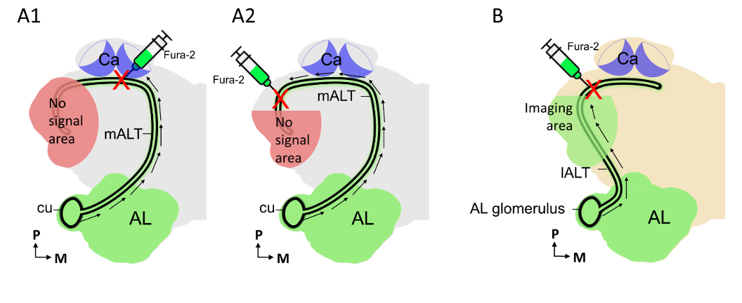
Figure(A1-A2): Fura retrograde labeling of PNs confined to the medial tract (mALT) from two different brain cites in moth. Figure B: Fura retrograde labeling of lateral-tract (lALT) PNs in honeybee brain. Calcium imaging measurements are feasible in the areas marked in green, including the antennal lobe (AL in A-B) and a part of lateral protocerebrum region (B). While the areas marked in red (shown in A1-A2) are not ideal for imaging experiment, as the neuronal signals (black arrows) will be physically blocked by the damaged axons.
In addition, the reviewer has the following objection: “Although the authors characterize morphologically and functionally a considerable number of neurons, the data are highly descriptive and exhibit a rather large level of variability which impedes, in my opinion, a generalization of response properties for different neuron types.” We assume the reviewer refers to the individual neuron data when he/she points out the relatively high variability. Indeed, the high-resolution information obtained by the intracellular recording/staining technique include descriptive data with a certain extent of variability – particularly regarding the spiking data representing every single action potential at the time scale of a few milliseconds. The main reason for performing both in vivo calcium imaging and intracellular recording experiments is that these two approaches form an optimal combination of illustrating the neuronal activity in different granularities. During calcium imaging, we recorded pheromone responses in distinct groups of MGC PNs, i.e., at a higher population scale. One main restriction of calcium imaging is the low temporal resolution (sampling frequency in this study was 100 ms). For comparison, the intracellular recordings had a sampling frequency less than 1 ms. Altogether, by combining the two techniques we could collect data from the relevant MGC-PNs both at the neuron population level (low temporal resolution) and single neuron level (high spatial and temporal resolution). Comparison of the data obtained from the two experimental approaches demonstrated a high degree of correspondence. We believe that the high-resolution intracellular recording data reflect the peculiar features that precisely characterize individual neurons. Otherwise, in case the reviewer has objections against the detailed descriptions in the results part, we have revised the original manuscript (including text and figure material) emphasizing on the main findings and minimizing the description of details.
The reviewer also suggests registering the neurons into a standard brain framework to “allow drawing a general picture about how coding of pheromones in the individual MGC compartments of the AL is transformed into a representation in higher brain centers”. To register individual PNs into a standard brain is no doubt an ideal method to compare the neurons’ architecture within the same species as well as across different models – especially if we want to compare the neurons’ projection patterns. Unlike the honeybee and the fruit fly already having an averaged standard brain available (reconstructed and standardized based on morphological data from different individuals), H. armigera has a representative brain (reconstructed from morphological data of one individual), published by Chu et al., (2020a). As we have experienced, errors due to local distortions often occur when registering neurons into a representative brain. The same is to some degree also the case for registration of neurons into an averaged brain framework. How informative the results are, will always depend both on the resolution of the standard and the resolution of the neuron data. Thus, the accuracy and the quality of the registration is based on the richness of details in the raw image data, i.e. how dense the registration grid is. If only a few neuropils are used, the precision of registration will obviously be limited. An ideal reconstruction for registration would include a dense grid of landmarks - or, as in the fruit fly, the actual image data.
Generally, the terminal projections of medial- and mediolateral tract MGC PNs in the moth cover several widespread areas in the protocerebrum and the most important objective of the current study was to map the neuropils innervated by each of the 32 physiologically identified neurons presented here. In line with the suggestion from the reviewer, we have added AMIRA reconstructions in the revised manuscript, including not only the skeleton of individual PNs but also 3D reconstructions of the neuropil regions innervated by each neuron. These data, confirming the neurons’ morphological properties, are presented in the figure supplement. In addition, for visualization purposes, we plotted each traced skeleton onto the representative brain, based on the reconstructed data obtained by using the ‘transform editor’ function in AMIRA (Fig. 3). In the revised version of the manuscript, we have also submitted all morphological data (confocal stacks and 3D-AMIRA reconstructions) of the main MGC-PN types to the newly established Insect brain database (InsectbrainDB, 2021) – a unified and open access platform for archiving and sharing functional data obtained not only from H. armigera but from other insect species as well.
In addition to registering different PNs into a common frame, another reliable evidence for such comparison is raw confocal data including identifiable neurons simultaneously stained in the same brain. In Fig. 3C, we demonstrate overlapping terminal projections in the LH of two uniglomerular MGC-PNs originating from each of the two smaller MGC-units, the dma and dmp. And in Fig. 4, we show the terminal projections of MGC-PNs confined to each of the three main tracts, demonstrating overlapping terminal arbors for medial- and mediolateral-tract neurons whereas the lateral-tract neuron projects to a separate area.
Reviewer #3:
Summary of goals:
In the moth Helicoverpa armigera the authors examined whether projection neurons from different antennal lobe tracts encoding sex-pheromone components with different valence occupy distinct projection areas in the protocerebrum of the midbrain.
Strengths and weaknesses of methods and results:
Methods chosen are adequate and state of the art. In vivo calcium imaging allowed for more easy imaging of a population of neurons, in search for statistically significant responses to pheromone components of different concentrations, quality, and valence. The main, general drawbacks of calcium imaging is the lower temporal resolution that does not allow for detection of single action potentials at the scale of few ms and the inability of fine spatial resolution of projection patterns of single neurons. This was compensated for by excellent intracellular recordings of single antennal lobe projection neurons, stainings of single cells, and embedding in the 3D standardized H. armigera brain. The data a very carefully analyzed with adequate analysis software and adequate statistical analysis and the most relevant results are shown in very good Figures. I also very much appreciate all of the supplementary figures. I do not see any relevant weakness in the methods and the respective results. However, as outlined in detail in the reply to the authors, the wording of the manuscript can be improved, to make it clearer and understandable without the need to read previous publications.
Everybody working with odors knows about the difficulty to precisely control and measure the exact molar concentration of odorants applied. But since the authors showed in previous publications that they take great care to control odor stimuli they should include also in the Material and Methods of this publication more details about concentration of the respective odor stimuli or mixtures employed.
Did they achieve their aims? Do data support conclusions?
Yes, the data support their conclusions as clearly shown in their excellent recordings, their excellent combination of physiological and morphological analysis, as well as their thorough statistical analysis.
Discussion of the likely impact of the work on the field, utility of methods:
This is an excellent, synergistic collaboration of different international experts in insect olfaction. It is still under-estimated how important the combination of single cell analysis in intracellular recordings with neural network analysis via calcium imaging is. Schemes of frequency encoding versus temporal encoding can only be deciphered with a clever combination of these techniques. This manuscript adds important insights into information processing of olfactory stimuli of antagonistic valence. It starts to become clear that in different sensory systems valence of aversive versus attractive sensory stimuli is processed in parallel pathways. Most likely antagonistic pathways connected to different neuronal units in premotor areas of the midbrain, connecting to parallel de- and ascending pathways of central pattern generators in the thorax. In addition, the current work provides relevant new information about processing of pheromone information in the different antennal lobe tracts in another important species. Thus, we may be one step closer to the future manipulation of sexual reproduction of specific insect pests.
Context for others for interpretations:
Sympatric heliothine moths use the same sex-pheromone components but at different concentration ratios, allowing for distinction of species that do not inter-mate. Thus, understanding how pheromone components at defined concentrations with opposite valence are processed in the brain to guide aversive or attractive behavioral interactions is relevant not only for determining principles of higher-order olfactory processing, but also to understand evolution of new species.
We thank the reviewer for the comments and suggestions. To improve the part of the manuscript covering background information, we have included a new figure in the introduction section, Fig. 1, providing an overview of the olfactory pathway in male moths. Here, the schematic drawing (A) contains an overview of the uniglomerular medial-tract PNs confined to the plant-odor and pheromone sub-system, respectively, and their distinct paths from the periphery to higher olfactory centers. In the schematic drawing (B), we provide an overview of the three main ALTs in the moth. A detailed description of the system is included in the relevant figure legend. In addition, we have included a section in the discussion that compares morphological and physiological properties of MGC-PNs confined to each of the three parallel tracts. Finally, a consideration implying the distinct roles of the parallel ALTs is added.
As suggested by the reviewer, we have added more precise information about the relevant odor stimuli in the revised version of the manuscript. We have clarified all details regarding pheromone concentrations as well as ratios in the materials and method section. In addition, we included relevant background knowledge on species-specific pheromone blends of sympatric moth species.
Author Response
Reviewer #1 (Public Review):
This work sheds light on the adverse effects of Bacillus thuringiensis, a strong pathogenic bacteria used as a microbial pesticide to kill lepidopteran larvae that threaten crops, on gut homeostasis of non-susceptible organisms. By using the Drosophila melanogaster as a non-susceptible organism model, this paper reveals the mechanisms by which the bacteria disrupt gut homeostasis. Authors combined the use of different genetic tools and Western blot experiments to successfully demonstrate that bacterial protoxins are released and activated throughout the fly gut after ingestion and influence intestinal stem cell proliferation and intestinal cell differentiation. This phenomenon relies on the interaction of activated protoxins with specific components of adherens junctions within the intestinal epithelium. Due to conserved mechanisms governing intestinal cell differentiation, this work could be the starting point for further studies in mammals.
The conclusions proposed by the authors are in general well supported by the data. However, some improvements in data representation, as well as additional key control experiments, would be needed to further reinforce some key points of the paper.
We thank reviewer1 for her appreciation of the work and in depth analysis of the data. We agree with all her comments and believe the suggestions significantly improved the manuscript.
1) Figure 1 and others: Several graphs in the manuscript show the number of cells/20000µm2. How is the shape of the gut in the different conditions studied in this manuscript? The gut shape (shrunk gut versus normal gut for example) could influence the number of cells seen in a small area. For example, the number of total cells quantified in a small area (here 20000µm2) of a shrunk gut can be increased while their size decrease. As a result, the quantification of a specific cell type in a small region (here 20000µm2) can be biased and not represent the real number of cells present in the whole posterior part of the R4 region. Would it make sense to calculate a ratio "number of X cells/number of DAPI positive cells per 20000µm2"?
We provided a suitable answer in the "Essential Revisions point 1" corresponding to this reviewer's concern. To summarize, we have now added whole posterior midgut images in the different conditions to highlight the intestinal morphology (Figure 1-figure supplement 1A). The whole gut morphology was not affected by the different challenges we performed. Indeed, we used low doses of spores and/or toxins in order to mimic "natural" amounts of spores/toxins the fly can eat in the environment and in order to avoid drastic gut lining disturbances.
We have also added the cell type ratio in figure 1- figure supplement 2.
2) Figure 4: Is it possible that Arm staining is less intense between ISC and progenitors after ingestion of the bacteria due to the fact there is a high rate of stem cell proliferation? Could it be an indirect effect of stem cell proliferation rather than the binding of the toxins to Cadherins?
We thank the reviewer for this pertinent comment. Indeed, for this reason, we compared the intensity of Arm expression at the junction between neighboring progenitors with the Arm intensity around the rest of the cellular membranes and calculated the ratio between both values (see Figure 4-figure supplement 1F-G for an illustration of how we proceeded and the new section in the Material and Methods 736-742). Using this method, even if the whole Arm staining intensity is different (in all the midgut), the ratio reflects the internal cell-cell interaction changes between the two neighboring cells. Moreover, we have observed that Arm staining (using the usual monoclonal antibody N2 7A1 from the DSHB) was very variable from one midgut to another in the same feeding/intoxication condition. So, we do not want to draw conclusion about the whole Arm intensity due to this variability whatever are the intoxication conditions. Finally, the challenged guts always displayed a more disorganized epithelium due to cell proliferation and differentiation. Consequently, Arm staining in ECs and progenitor cells are found in the same focal plane while in unchallenged and well-organized guts, Arm staining in ECs is above the focal plane of Arm staining in progenitor cells. This likely leads to the impression that Arm staining is more intense in challenged midguts. This method description is now added in the Material and methods section (lines 736-742).
Could the authors use the ReDDM system to distinguish between "old" and newly formed cells? This could be a good control to make sure that the signal is quantified in similar cells between the control and the different conditions.
We have analyzed intensity of Arm expression between pairs of GFP cells. Most of these pairs arose from de novo divisions. Indeed, as shown in control conditions (water) with Dl-ReDDM (for example see figure 1-figure supplement 1D), pairs of GFP cells (ISC-ISC) are rare. Most pairs correspond to ISC-EB or ISC-EEP pairs with the progenitor marked by the RFP, meaning that it just arises from the GFP+ mother ISC. Therefore we assume, that in the esg>GFP genotype, pairs of GFP+ cells correspond to one ISC and one progenitor (see Figure 4 – figure supplement 1A-A'). Therefore, when we analyzed the Arm intensity between pairs of GFP cells after intoxication, these cells are very likely "newborn" cells. Even if we suppose there are ISCs and progenitors that remain stuck together for a long time (for instance several days), Cry1A toxins can also be able to disrupt their cell junction. In the context of Cry1A toxin activity, it seems important to analyze the whole impact on cell-cell junctions without discriminating old and new cell-cell interactions.
We tried to use anti-Arm and anti-Pros double staining to mark new EEPs. Unfortunately, anti-Arm and anti-Prospero antibodies were both raised in mice. Co-staining with both antibodies give rise to bad labelling either for Arm or for Prospero or for both. Our first author spent lot of energy trying to set up good conditions but unfortunately this was unsuccessful.
Here is an example of what we got (this was the best image we got) with esg>GFP flies fed with water (control) and labelled for Arm and Pros in red. White arrows point two EEPs. Red arrows points the Arm staining between two precursors (ISC/ISC or ISC/EB or EB/EB). It was extremely hard to identify junctions marked by Arm between EEPs and ISCs because the Pros staining was too strong.
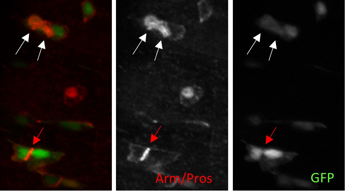
Another example with flies fed with spores of SA11 (increasing the number of EEs). In green is the esg>GFP and in Red Arm and Prospero. The right panel correspond to the single red channel (Arm/Prospero).
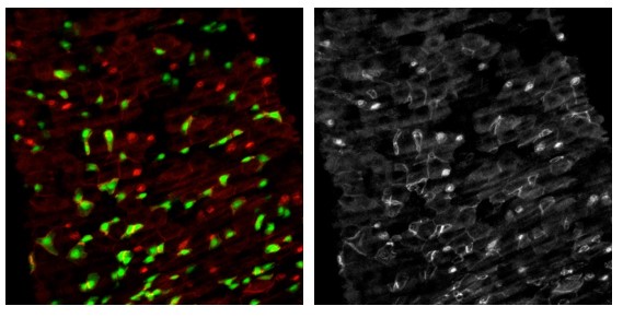
Nevertheless, we have now performed a similar analysis in an esg>GFP, Shg::RFP background and analyzed Shg::RFP (Tomato::DE-Cadherin) labelling intensity. We found similar results that are presented in the new Figure 4 (data we Arm have been moved in Figure 4-figure supplement 1). This last analysis have been included in the text lines 285-299.
Figure 4E' and 4G': Arm staining seems more intense when looking at the whole membrane levels of cells compared to control. Is it possible that the measured ratio contact intensity/membrane intensity presented in Figure 4I could be impacted and not reflect the real contact intensity between ISC and progenitor cells?
Please check our answer just above: "…//… we have observed that Arm staining (using the usual monoclonal antibody N2 7A1 from the DSHB) was very variable from one midgut to another in the same feeding/intoxication condition. So, we do not want to draw conclusion about the whole Arm intensity due to this variability whatever are the intoxication conditions".
See also our intensity measurement method described above to avoid bias: "…//… we compared the intensity of Arm expression at the junction between neighboring progenitors with the Arm intensity around the rest of the cellular membranes and calculated the ratio between both values (see Figure 4-figure supplement 1F-G for an illustration of how we proceeded and the new section in the Material and Methods 736-742). Using this method, even if the whole Arm staining intensity is different (in all the midgut), the ratio reflects the internal cell-cell interaction changes between the two neighboring cells."
What is the hypothesis of the authors about the decrease of Arm or DE-Cad seen after bacterial/crystal ingestion? Does the interaction between the toxins and DE-Cad induce a relocation of DE-Cad?
It has been shown that E-Cadherin could be recycled when adherens junctions are destabilized both in Drosophila and mammals(Buchon et al., 2010; O'Keefe et al., 2007; Tiwari et al., 2018). To investigate this possibility, we tried to analyze DE-Cad cytoplasmic relocalization using anti-DE-Cad immunostaining (DCAD2 antibody from DSHB) as well as Shg::RFP (Bloomington stock #58789) or Shg::GFP (Bloomington stock #60584) endogenous fusion. Unfortunately, we did not see obvious differences. Nevertheless, we have now added the split channels of the Shg::RFP labelling in the different conditions in Figure 4A-D'. Nevertheless, we are still interested in the behavior of the DE-cadherin (and signaling, see (Liang et al., 2017)) upon binding of the Cry1A toxin. N. Zucchini-Pascal (author in this article) are currently investigating this question.
The authors should add more details about the way to quantify in the Material and methods section. How many cells have been quantified per intestine? How did they choose the cells where they quantified the contact intensity?..etc
These details were missing in the methods and we thank the reviewer for highlighting this issue. We added these information to the methods (lines 725-742). The number of cell pairs analyzed was present in the raw data related to figure 4 but absent from the main figure and legend. It is now rectified. We only measured the intensity in isolated pairs of cells.
Figure 4B, D, F and H: How did the authors recognize the ISCs?
We agree with the reviewer comment. We cannot recognize ICS per se. Green cells correspond either to ISCs or to EBs. We modified the text accordingly (lines 285-287).
Could the authors do quantifications of DE-Cad signal?
This has been done. It is shown now in figure 4E and in Table 1. We also adapted the text (lines 289-299) to fine-tune our interpretation in light of this new analysis. Indeed, what we have now defined as "mild" adherens junction intensity is between the ratio 1.4 and 1.6 instead of the previous ratio (1.3 to 1.6), because we observed most of the EEP progenitors arising from cell displaying a junction intensity with their mother cells below the 1.4 ratio (see Table 1).
Like Arm staining, the staining seems stronger at the whole membrane level in F and H compared to the control.
As we described above for Arm staining, the intensity of Tomato::DE-Cad labelling can differ from one posterior midgut to another one. One simple explanation would be related to changes in the structure of midgut epithelium which is well organized in unchallenged conditions, while in challenged midguts the epithelial cells are not well-arranged anymore due to rapid cell proliferation and differentiation. Consequently, DE-Cad labelling in ECs is at the same level as that in ISC/progenitors cells, giving the impression that the labelling is stronger.
3) Figure 5: How is the stem cell proliferation upon overexpression of DE-Cad in control or upon bacteria/crystals ingestion? Do the authors think that the decrease of Pros+RFP+ new cells upon overexpression of DE-Cad could result from a decrease of stem cell proliferation?
Great suggestion. Thereby, we chose to count the progenitor cells (GFP+ cells) reflecting the ISC division during the last 3 days. Moreover, this also has the advantage of working on the same pictures (samples) used for all the analyzes shown in figure 5 and Figure 5-figure supplement 1. Hence, If we consider the number of GFP+ cells (esg expressing cells corresponding to ISC, EB or EEP) in challenged midguts, the overexpression of the DE-Cad did not seem to alter ISC division. In addition, we still observed more GFP+ cells when the midguts were challenged with SA11 or crystals than with BtkCry, in agreement with the rate of ISC division observed in the WT genetic background shown in figure 1B.
We have now added the counting of GFP+ cells in Figure 5-figure supplement 1E. The text has been modified to integrate this results (lines 306-308).
Did the authors quantify the % of new ECs in the context of overexpression of DE-Cad?
The data has been added in figure 5F. The text has been modified to integrate this result lines 312-313.
Figure 5F: As asked before, did the authors distinguish the signal between newly born cells and the signal between older cells?
In the new figure 5G: we used the esg-ReDDM system that is very efficient. Almost all ISC and progenitors express the GFP. The counting have been done between cell pairs that express both the GFP and RFP. It is specified in the text lines 310-311. Nevertheless, we cannot distinguish between new and old cells here. Indeed, the esg-ReDDM system induce both the GFP and the RFP in all esg+ cells (the old ones and the new ones). Hence, if a division has occurred just before the induction of the system to give birth for instance to an ISC and an EB, both cells will express the GFP and the RFP. But should we consider those pairs of cells as old cells or new cells? Noteworthy, as we analyzed the intensity of junctions 3 days after intoxication and induction of the ReDDM system, we assume that the pairs of GFP+/RFP+ cells arose after the induction of the system. Indeed, to our knowledge, nobody has shown in the posterior midgut, that a progenitor remains stuck to its mother ISC as long as 3 days. Even if we assume that this event can occur, Cry1A toxins can also be able to disrupt their cell junction.
We now have removed the DAPI channel and added the RFP+ channel in Figure 5-figure supplement 1A-D' (previously the Figure S4A-D) to illustrate this explanation and to facilitate the interpretation by the reader.
It would be interesting to compare the junction intensity between mother ISCs and their daughter progenitors before and after intoxication in a same intestine. But we think that this event is quite rare because of the experimental conditions we used (i.e. analyses 3 days after the induction of the ReDDM/intoxication).
The same experiments (stem cell proliferation + quantification of the % of new ECs) could be also done when authors overexpress of the Connectin, supplemental figure 5. This would be another control to conclude that the effects on cell differentiation are specific due to the interaction between DE-Cad and the toxins.
We have added the analyses in Figure 5 - figure supplement 2J and K.
The text has been completed lines 317-320.
In the "crystals" condition, the overexpression of Connection seems to partially rescue the increase % of new Pros+RFP+ new cells observed in Figure 3F (Figure S5I compared to Figure 3F).
Yes, we agree with the reviewer comment. In an esg-ReDDM background (figure 3F), crystals induced a much greater increase in EE numbers than did SA11 spores. However, in a WT or esg>GFP background, crystals induced a similar increase in EE/EEP to that induced by SA11 spores. So we do not yet have explanation excepted the genetic background of the esg-ReDDM.
Author Response
Reviewer #1 (Public Review):
The authors start the study with an interesting clinical observation, found in a small subset of prostate cancers: FOXP2-CPED1 fusion. They describe how this fusion results in enhanced FOXP2 protein levels, and further describe how FOXP2 increases anchorageindependent growth in vitro, and results in pre-malignant lesions in vivo. Intrinsically, this is an interesting observation. However, the mechanistic insights are relatively limited as it stands, and the main issues are described below.
Main issues:
1) While the study starts off with the FOXP2 fusion, the vast majority of the paper is actually about enhanced FOXP2 expression in tumorigenesis. Wouldn't it be more logical to remove the FOXP2 fusion data? These data seem quite interesting and novel but they are underdeveloped within the current manuscript design, which is a shame for such an exciting novel finding. Along the same lines, for a study that centres on the prostate lineage, it's not clear why the oncogenic potential of FOXP2 in mouse 3T3 fibroblasts was tested.
We thank the reviewer very much for the comment. We followed the suggestion and added a set of data regarding the newly identified FOXP2 fusion in Figure 1 to make our manuscript more informative. We tested the oncogenic potential of FOXP2 in NIH3T3 fibroblasts because NIH3T3 cells are a widely used model to demonstrate the presence of transformed oncogenes2,3. In our study, we observed that when NIH3T3 cells acquired the exogenous FOXP2 gene, the cells lost the characteristic contact inhibition response, continued to proliferate and eventually formed clonal colonies. Please refer to "Answer to Essential Revisions #1 from the Editors” for details.
2) While the FOXP2 data are compelling and convincing, it is not clear yet whether this effect is specific, or if FOXP2 is e.g. universally relevant for cell viability. Targeting FOXP2 by siRNA/shRNA in a non-transformed cell line would address this issue.
We appreciate these helpful comments. Please refer to the "Answer to Essential Revisions #1 from the Editors” for details.
3) Unfortunately, not a single chemical inhibitor is truly 100% specific. Therefore, the Foretinib and MK2206 experiments should be confirmed using shRNAs/KOs targeting MEK and AKT. With the inclusion of such data, the authors would make a very compelling argument that indeed MEK/AKT signalling is driving the phenotype.
We thank the reviewer for highlighting this point and we agree with the reviewer’s point that no chemical inhibitor is 100% specific. In this study, we used chemical inhibitors to provide further supportive data indicating that FOXP2 confers oncogenic effects by activating MET signaling. We characterized a FOXP2-binding fragment located in MET and HGF in LNCaP prostate cancer cells by utilizing the CUT&Tag method. We also found that MET restoration partially reversed oncogenic phenotypes in FOXP2-KD prostate cancer cells. All these data consistently supported that FOXP2 activates MET signaling in prostate cancer. Please refer to the "Answer to Essential Revisions #2 from the Editors” and to the "Answer to Essential Revisions #7 from the Editors” for details.
4) With the FOXP2-CPED1 fusion being more stable as compared to wild-type transcripts, wouldn't one expect the fusion to have a more severe phenotype? This is a very exciting aspect of the start of the study, but it is not explored further in the manuscript. The authors would ideally elaborate on why the effects of the FOXP2-CPED1 fusion seem comparable to the FOXP2 wildtype, in their studies.
We thank the reviewer very much for the comment. We had quantified the number of colonies of FOXP2- and FOXP2-CPED1-overexpressing cells, and we found that both wildtype FOXP2 and FOXP2-CPED1 had a comparable putative functional influence on the transformation of human prostate epithelial cells RWPE-1 and mouse primary fibroblasts NIH3T3 (P = 0.69, by Fisher’s exact test for RWPE-1; P = 0.23, by Fisher’s exact test for NIH3T3). We added the corresponding description to the Results section in Line 487 on Page 22 in the tracked changes version of the revised manuscript. Please refer to the "Answer to Essential Revisions #5 from the Editors” for details.
5) The authors claim that FOXP2 functions as an oncogene, but the most-severe phenotype that is observed in vivo, is PIN lesions, not tumors. While this is an exciting observation, it is not the full story of an oncogene. Can the authors justifiably claim that FOXP2 is an oncogene, based on these results?
We appreciate the comment, and we made the corresponding revision in the revised manuscript. Please refer to the "Answer to Essential Revisions #3 from the Editors” for details.
6) The clinical and phenotypic observations are exciting and relevant. The mechanistic insights of the study are quite limited in the current stage. How does FOXP2 give its phenotype, and result in increased MET phosphorylation? The association is there, but it is unclear how this happens.
We appreciate this valuable suggestion. In the current study, we used the CUT&Tag method to explore how FOXP2 activated MET signaling in LNCaP prostate cancer cells, and we identified potential FOXP2-binding fragments in MET and HGF. Therefore, we proposed that FOXP2 activates MET signaling in prostate cancer through its binding to MET and METassociated gene. Please refer to the "Answer to Essential Revisions #2 from the Editors” for details.
Reviewer #2 (Public Review):
1) The manuscript entitled "FOXP2 confers oncogenic effects in prostate cancer through activating MET signalling" by Zhu et al describes the identification of a novel FOXP2CPED1 gene fusion in 2 out of 100 primary prostate cancers. A byproduct of this gene fusion is the increased expression of FOXP2, which has been shown to be increased in prostate cancer relative to benign tissue. These data nominated FOXP2 as a potential oncogene. Accordingly, overexpression of FOXP2 in nontransformed mouse fibroblast NIH-3T3 and human prostate RWPE-1 cells induced transforming capabilities in both cell models. Mechanistically, convincing data were provided that indicate that FOXP2 promotes the expression and/or activity of the receptor tyrosine kinase MET, which has previously been shown to have oncogenic functions in prostate cancer. Notably, the authors create a new genetically engineered mouse model in which FOXP2 is overexpressed in the prostatic luminal epithelial cells. Overexpression of FOXP2 was sufficient to promote the development of prostatic intraepithelial neoplasia (PIN) a suspected precursor to prostate adenocarcinoma and activate MET signaling.
Strengths:
This study makes a convincing case for FOXP2 as 1) a promoter of prostate cancer initiation and 2) an upstream regulator of pro-cancer MET signaling. This was done using both overexpression and knockdown models in cell lines and corroborated in new genetically engineered mouse models (GEMMs) of FOXP2 or FOXP2-CPED1 overexpression in prostate luminal epithelial cells as well as publicly available clinical cohort data.
Major strengths of the study are the demonstration that FOXP2 or FOXP2-CPED1 overexpression transforms RWPE-1 cells to now grow in soft agar (hallmark of malignant transformation) and the creation of new genetically engineered mouse models (GEMMs) of FOXP2 or FOXP2-CPED1 overexpression in prostate luminal epithelial cells. In both mouse models, FOXP2 overexpression increased the incidence of PIN lesions, which are thought to be a precursor to prostate cancer. While FOXP2 alone was not sufficient to cause prostate cancer in mice, it is acknowledged that single gene alterations causing prostate cancer in mice are rare. Future studies will undoubtedly want to cross these GEMMs with established, relatively benign models of prostate cancer such as Hi-Myc or Pb-Pten mice to see if FOXP2 accelerates cancer progression (beyond the scope of this study).
We appreciate these positive comments from the reviewer. We agree with the suggestion from the reviewer that it is worth exploring whether FOXP2 is able to cooperate with a known disease driver to accelerate the progression of prostate cancer. Therefore, we are going to cross Pb-FOXP2 transgenic mice with Pb-Pten KO mice to assess if FOXP2 is able to accelerate malignant progression.
2) Weaknesses: It is unclear why the authors decided to use mouse fibroblast NIH3T3 cells for their transformation studies. In this regard, it appears likely that FOXP2 could function as an oncogene across diverse cell types. Given the focus on prostate cancer, it would have been preferable to corroborate the RWPE-1 data with another prostate cell model and test FOXP2's transforming ability in RWPE-1 xenograft models. To that end, there is no direct evidence that FOXP2 can cause cancer in vivo. The GEMM data, while compelling, only shows that FOXP2 can promote PIN in mice and the lone xenograft model chosen was for fibroblast NIH-3T3 cells.
To determine the oncogenic activity of FOXP2 and the FOXP2-CPDE1 fusion, we initially used mouse primary fibroblast NIH3T3 for transformation experiments, because NIH3T3 cells are a widely used cell model to discover novel oncogenes2,3,10,11. Subsequently, we observed that overexpression of FOXP2 and its fusion variant drove RWPE-1 cells to lose the characteristic contact inhibition response, led to their anchorage-independent growth in vitro, and promoted PIN in the transgenic mice. During preparation of the revised manuscript, we tested the transformation ability of FOXP2 and FOXP2-CPED1 in RWPE1 xenograft models. We subcutaneously injected 2 × 10⁶ RWPE-1 cells into the flanks of NOD-SCID mice. The NODSCID mice were divided into five groups (n = 5 mice in each group): control, FOXP2overexpressing (two stable cell lines) and FOXP2-CPED1- overexpressing (two cell lines) groups. The experiment lasted for 4 months. We observed that no RWPE-1 cell-injected mice developed tumor masses. We propose that FOXP2 and its fusion alone are not sufficient to generate the microenvironment suitable for RWPE-1-xenograft growth. Collectively, our data suggest that FOXP2 has oncogenic potential in prostate cancer, but is not sufficient to act alone as an oncogene.
3) There is a limited mechanism of action. While the authors provide correlative data suggesting that FOXP2 could increase the expression of MET signaling components, it is not clear how FOXP2 controls MET levels. It would be of interest to search for and validate the importance of potential FOXP2 binding sites in or around MET and the genes of METassociated proteins. At a minimum, it should be confirmed whether MET is a primary or secondary target of FOXP2. The authors should also report on what happened to the 4-gene MET signature in the FOXP2 knockdown cell models. It would be equally significant to test if overexpression of MET can rescue the anti-growth effects of FOXP2 knockdown in prostate cancer cells (positive or negative results would be informative).
We appreciate all the valuable comments. As suggested, we performed corresponding experiments, please refer to the " Answers to Essential Revisions #2 from the Editors”, to the "Answer to Essential Revisions #6 from the Editors”, and to the "Answer to Essential Revisions #7 from the Editors” for details.
Reviewer #3 (Public Review):
1) In this manuscript, the authors present data supporting FOXP2 as an oncogene in PCa. They show that FOXP2 is overexpressed in PCa patient tissue and is necessary and sufficient for PCa transformation/tumorigenesis depending on the model system. Overexpression and knock-down of FOXP2 lead to an increase/decrease in MET/PI3K/AKT transcripts and signaling and sensitizes cells to PI3K/AKT inhibition.
Key strengths of the paper include multiple endpoints and model systems, an over-expression and knock-down approach to address sufficiency and necessity, a new mouse knock-in model, analysis of primary PCa patient tumors, and benchmarking finding against publicly available data. The central discovery that FOXP2 is an oncogene in PCa will be of interest to the field. However, there are several critically unanswered questions.
1) No data are presented for how FOXP2 regulates MET signaling. ChIP would easily address if it is direct regulation of MET and analysis of FOXP2 ChIP-seq could provide insights.
2) Beyond the 2 fusions in the 100 PCa patient cohort it is unclear how FOXP2 is overexpressed in PCa. In the discussion and in FS5 some data are presented indicating amplification and CNAs, however, these are not directly linked to FOXP2 expression.
3) There are some hints that full-length FOXP2 and the FOXP2-CPED1 function differently. In SF2E the size/number of colonies between full-length FOXP2 and fusion are different. If the assay was run for the same length of time, then it indicates different biologies of the overexpressed FOXP2 and FOXP2-CPED1 fusion. Additionally, in F3E the sensitization is different depending on the transgene.
We appreciate these valuable comments and constructive remarks. As suggested, we performed the CUT&Tag experiments to detect the binding of FOXP2 to MET, and to examine the association of CNAs of FOXP2 with its expression. Please refer to the " Answer to Essential Revisions #2 from the Editors" and the " Answer to Essential Revisions #4 from the Editors" for details. We also added detailed information to show the resemblance observed between FOXP2 fusion- and wild-type FOXP2-overexpressing cells. We added the corresponding description to the Results section in Line 487 on Page 22 in the tracked changes version of the revised manuscript. Please refer to the “Answer to Essential Revisions #5 from the Editors” for details.
2) The relationship between FOXP2 and AR is not explored, which is important given 1) the critical role of the AR in PCa; and 2) the existing relationship between the AR and FOXP2 and other FOX gene members.
We thank the reviewer very much for highlighting this point. We agree that it is important to examine the relationship between FOXP2 and AR. We therefore analyzed the expression dataset of 255 primary prostate tumors from TCGA and observed that the expression of FOXP2 was significantly correlated with the expression of AR (Spearman's ρ = 0.48, P < 0.001) (Figure 1. a). Next, we observed that both FOXP2- and FOXP2-CPED1overexpressing 293T cells had a higher AR protein abundance than control cells (Figure 1. b). In addition, shRNA-mediated FOXP2 knockdown in LNCaP cells resulted in a decreased AR protein level compared to that in control cells (Figure 1. c). However, we analyzed our CUT&Tag data and observed no binding of FOXP2 to AR (Figure 1. d). Our data suggest that FOXP2 might be associated with AR expression.
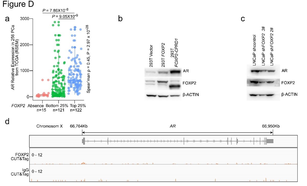
Figure 1. a. AR expression in a human prostate cancer dataset (TCGA, Prostate Adenocarcinoma, Provisional; n = 493) classified by FOXP2 expression level (bottom 25%, low expression, n = 120; top 25%, high expression, n = 120; negative expression, n = 15). P values were calculated by the MannWhitney U test. The correlation between FOXP2 and AR expression was evaluated by determining the Spearman's rank correlation coefficient. b. Immunoblot analysis of the expression levels of AR in 293T cells with overexpression of FOXP2 or FOXP2-CPED1. c. Immunoblot analysis of the expression levels of AR in LNCaP cells with stable expression of the scrambled vector or FOXP2 shRNA. d. CUT&Tag analysis of FOXP2 association with the promoter of AR. Representative track of FOXP2 at the AR gene locus is shown.
Reference
Author Response:
Reviewer #2 (Public Review):
In the paper entitled "The Oncoprotein BCL6 Enables Cancer Cells to Evade Genotoxic Stress", through comparing transcriptional profilings of ETO sensitive versus resistant tumor cell lines, the authors found that BCL6 was selectively upregulated in ETO-resistant tumor cells, and their further in vitro and in vivo data suggest that Bcl6 upregulation via the IFN-STAT1-Bcl6 axis conferred tumor resistance to genotoxic stress, and targeting Bcl6 significantly improved therapeutic efficacy of ETO/ADR in mouse tumor models.
Their findings are interesting and may inspire new combinational therapeutic strategy in treating chemotherapy resistant cancers, although a number of issues remain to be further clarified.
Major concerns:
- Through using in vitro assays, the authors defined a panel of genotoxic agents (ETO, ADR, etc) resistant or sensitive tumor cell lines, and indicated the resistance was caused by BCL6 upregulation. It was expected in the following on animal studies, the authors would choose tumor cell lines with clearly defined phenotypes characterized in their study. But it was not the cases in their studies. For examples, in Fig S2C and Fig 7B, the authors used an ambiguous tumor cell line HCT116 to test ETO resistance, which had only a borderline level of resistance to ETO (Fig 1A) but yet sensitive to ADR (Fig S1A), whereas in Fig 2H, the authors chose a tumor cell line (MCF7) not examined in their study, instead of the high ETO-resistant tumor cell lines H661/Capan-2 or high ADR-resistant cell lines DLD-1/H836.
We thank the reviewer very much for these insightful comments.
(1) We sincerely agree with the reviewer that our experiments should be carried out using cell lines that possess clear and potent resistance phenotype. However, some resistant cell lines (e.g., H661 and Capan-2) are hard to form tumors in mice according to published literature or our experiences. That’s why we initially chose the resistant cell line HCT116 for animal studies. To follow the reviewer’s suggestion and further validate our findings, in our revised manuscript, we additionally set up a tumor xenograft mouse model using PANC28 cells that are more resistant to etoposide than HCT116 cells. Our new data consistently showed that the BCL6 abundance in PANC28 xenografts was apparently increased by etoposide treatment, and as expected, BCL6 knockdown significantly sensitized etoposide. We have supplemented these new data in Figure 2D, Figure 2-figure supplement 1C and Figure 7C of our revised manuscript.
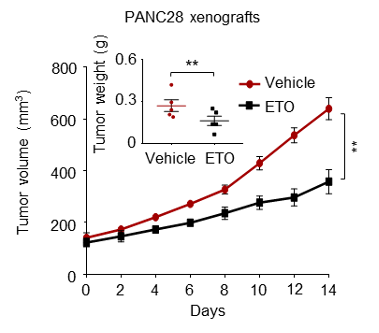
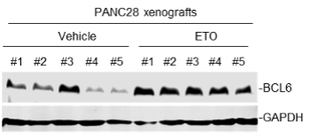
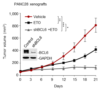
(2) Moreover, we also tested the in vitro sensitizing effects of BCL6 knockdown to etoposide and doxorubicin using Capan-2 and H838 cells that are much more resistant to genotoxic agents. As expected, our results showed that BCL6 genetic knockdown attenuated the clonogenic growth of these cells in the presence of etoposide or doxorubicin. We are sorry that we can't supplement all these figures in our revised manuscript due to limited space. We have added the Capan-2 data in our revised manuscript (Figure 2E).
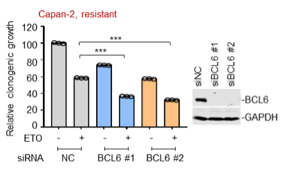
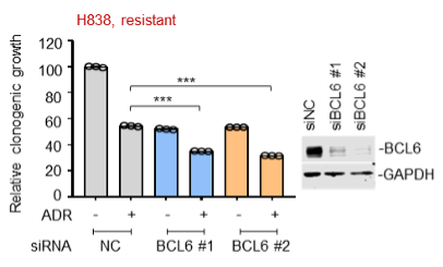
(3) In the previous version of our manuscript, we analyzed published datasets (Biomed Pharmacother. 2014 May;68(4):447-53; PLoS One. 2012;7(9):e45268), and found that BCL6 upregulation was also observed in cells with acquired chemoresistance (MCF7/ETO and A2780/ADR; Figure 1E). We further examined the inhibitory action of BCL6 silencing in the acquired chemo-resistant MCF7/ADR cells that we generated previously in our laboratory. Our results showed that BCL6 interference was sufficient to suppress the growth of MCF7/ADR cells. In attempting to make consistency of used cell lines across the experimental panels in our study, nevertheless, we decided to remove the MCF7/ADR proliferation data in our revised manuscript.
- Fig 3, the concept of tumor cell expressing IFNa/IFNg conferring genotoxic resistance sounds very interesting and novel, but the authors only tested IFNa/g expression at transcriptional level, protein expression data should be also provided.
We appreciate the reviewer’s comments.
In our study, we have examined the protein contents of IFN-α and IFN-γ using an ELISA assay. Our results showed that etoposide treatment led to a significant increase in IFN-α and IFN-γ contents in resistant cells. The results were expressed as fold change over the untreated control (Figure 3, H-I). We have revised the related figure legends to make it clearer to readers.
- Fig 3F-3I, ETO-induced interferon response should be examined comprehensively in different tumor cell lines as listed in Fig 1A/2A. Similarly, effect of exogenous IFNa/IFNg on ETO-resistance should be also examined comprehensively in both sensitive or resistant tumor cell lines. In addition, the effect of blocking IFNg/IFNa on ETO-resistance should be also tested in different tumor cell lines. These data are extremely useful for extending or strengthening the broad impact or influence of their findings.
We appreciate for the reviewer’s suggestion.
We agree that more cell lines should be examined in the context of exogenous addition of IFNα/IFNγ or IFNα/IFNγ blockade. However, it is hard for us to test all the cell lines as listed in Figure 1A/2A. In our revised manuscript, we expanded cell line panel in this part and supplemented several new data as listed below.
(1) In addition to the sensitive cell line H522 that has been already shown in our previous manuscript, we further tested PC9 cells and consistently found that exogenous addition of IFN-α and IFN-γ also protected PC9 cells from etoposide-induced cell death.
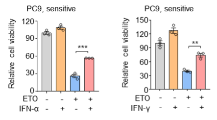
(2) In addition to the resistant cell line Capan-2 that has been already shown in our previous manuscript, we further tested H838 cells and consistently found that knockdown of the IFN-α receptor IFNAR1 led to an enhanced sensitivity of H838 cells to etoposide, as indicated by decreased IC50 values of etoposide and impaired clonogenic growth of H838 cells compared with the control group.
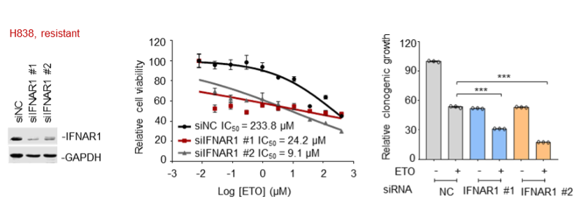
(3) In addition to the resistant cell line PANC28 that has been already shown in our previous manuscript, we further employed Capan-2 and H838 cells and consistently found that antibodies against IFN-γ also increased the killing ability of etoposide towards these resistant cells.
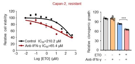
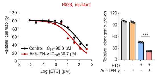
We are sorry that we can't supplement all these figures in our revised manuscript due to limited space. We have added the Capan-2 data in our revised manuscript (Figure 3O and Figure 3-figure supplement 1F).
- Fig 4A-L, the authors examined activation of IFN-STAT1-Bcl6 axis in tumor cells in different angles via different approaches, but using different tumor cell lines in different panels of experiments, making it quite annoying and difficult to judge their findings across different tumor cell lines. At least, ETO or IFNa/IFNg induced STAT1 upregulation and its phosphorylation should be examined comprehensively in both resistant and sensitive tumor cell lines.
We thank so much for this helpful comment.
We are so sorry for the inconsistency of cell lines used in our previous manuscript. We have employed consistent cell lines across the experimental panels and supplemented additional data in our revised manuscript. We chose the chemo-resistant cell line Capan-2, PANC28, H838 and HCT116 for mechanistic studies, and correspondingly, we employed the chemo-sensitive cell line H522, PC9 and PANC-1 for comparison in certain assays.
As suggested by the reviewer, we tested more cell lines to further elucidate the IFN-STAT1-Bcl6 axis. Our results showed that etoposide treatment promoted STAT1 abundance and its phosphorylated levels in etoposide-resistant Capan-2, PANC28 and H838 cells, but not in sensitive H522, PC9 and PANC-1 cells. Additionally, IFN-α and IFN-γ significantly led to a simultaneous increase in STAT1, phosphorylated STAT1 and BCL6 expression in the same resistant cell panel.
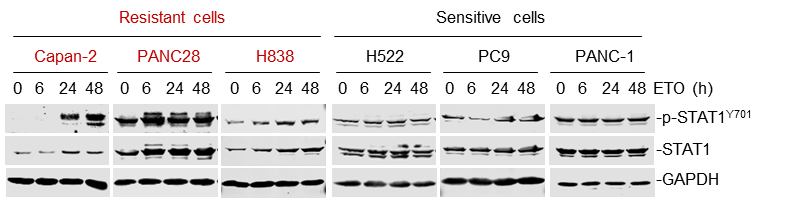
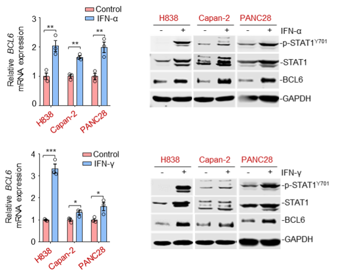
We have supplemented the new data in Figure 4A and Figure 4, C-F of our revised manuscript.
Author Response:
Reviewer #1:
In this paper, Alhussein and Smith set out to determine whether motor planning under uncertainty (when the exact goal is unknown before the start of the movement) results in motor averaging (average between the two possible motor plans) or in performance optimization (one movement that maximizes the probability of successfully reaching to one of the two targets). Extending previous work by Haith et al. with two new, cleanly designed experiments, they show that performance optimization provides a better explanation of motor behaviour under uncertainty than the motor averaging hypothesis.
We thank the reviewer for the kind words.
1) The main caveat of experiment 1 is that it rules out one particular extreme version of the movement averaging idea- namely that the motor programs are averaged at the level of muscle commands or dynamics. It is still consistent with the idea that the participant first average the kinematic motor plans - and then retrieve the associated force field for this motor plan. This idea is ruled out in Experiment 2, but nonetheless I think this is worth adding to the discussion.
This is a good point, and we have now included it in the paper as suggested – both in motivating the need for Expt 2 in the Results section and when interpreting the results of Expt 1 in the Discussion section.
2) The logic of the correction for variability between the one-target and two-target trials in Formula 2 is not clear to me. It is likely that some of the variability in the two-target trials arises from the uncertainty in the decision - i.e. based on recent history one target may internally be assigned a higher probability than the other. This is variability the optimal controller should know about and therefore discard in the planning of the safety margin. How big was this correction factor? What is the impact when the correction is dropped ?
Short Answer:
(1) If decision uncertainty contributed to motor variability on 2-target trials as suggested, 2-target trials should display greater motor variability than 1-target trials. However, 1-target and 2-target trials display levels of motor variability that are essentially equal – with a difference of less than 1% overall, as illustrated in Fig R2, indicating that decision uncertainty, if present, has no clear effect on motor variability in our data.
(2) The sigma2/sigma1 correction factor is, therefore, very close to 1, with an average value of 1.00 or 1.04 depending on how it’s computed. Thus, dropping it has little impact on the main result as shown in Fig R1.
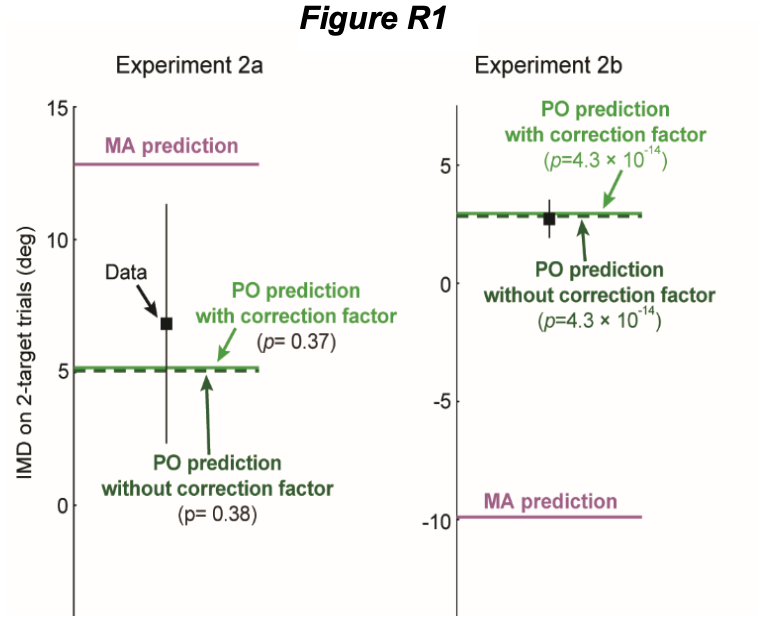
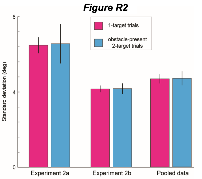
Longer, more detailed, answer:
We agree that it could be reasonable to think that if it were true that motor variability on 2-target trials were consistently higher than that on 1-target trials, then the additional variability seen on 2-target trials might result from uncertainty in the decision which should not affect safety margins if the optimal controller knew about this variability. However, detailed analysis of our data suggests that this is not the case. We present several analyses below that flush this out.
We apologize in advance that the response we provide to this seemingly straightforward comment is so lengthy (4+ pages!), especially since capitulating to the reviewer’s assertion that “correction” for the motor variability differences between 1 & 2-target trails should be removed from our analysis, would make essentially no difference in the main result, as shown Fig R1 above. Note that the error bars on the data show 95% confidence intervals. However, taking the difference in motor variability (or more specifically, it’s ratio) between 1-target and 2-target trials into account, is crucial for understanding inter-individual differences in motor responses in uncertain conditions. As this reviewer (and reviewer 2) points out below, we did a poor job of presenting the inter-individual differences analysis in the original version of this paper, but we have improved both the approach and the presentation in the current revision, and we think that this analysis is important, despite being secondary to the main result about the group-averaged findings.
Therefore, we present analyses here showing that it is unlikely that decision uncertainty accounts for the individual-participant variability differences we observe between 1-target and 2-target trials in our experiments (Fig R2). Instead, we show that the variability differences we observe in different conditions for individual participants are due to (largely idiosyncratic) spatial differences in movement direction (Fig R3), which when taken into account, afford a clearly improved ability to predict the size of the safety margins around the obstacles, both in 1-target trials where there is no ‘decision’ to be made (Figs R4-R6) and in 2-target trials (Figs R5-R6).
Variability is, on average, nearly identical on 1-target & 2-target trials, indicating no measurable decision-related increase in variability on 2-target trials
At odds with the idea that decision uncertainty is responsible for a meaningful fraction of the 2-target trial variability that we measure, we find that motor variability on 2-target trials is essentially unchanged from that on one-target trials overall as shown in Fig R2 (error bars show 95% confidence intervals). This is the case for both the data from Expt 2a (6.59±0.42° vs 6.70±0.96°, p > 0.8), and for the critical data from Expt 2b that was designed to dissociate the MA hypothesis from the PO hypothesis (4.23 ±0.17° vs 4.23±0.27°, p > 0.8 for the data from Expt 2b), as well as when the data from Expts 2a-b are pooled (4.78±0.24° vs 4.81±0.35°, p > 0.8). Note that the nominal difference in motor variability between 1-target and 2-target trials was just 1.7% in the Expt 2a data, 0.1% in the Expt 2b data, and 0.6% in the pooled data. This suggests little to no overall contribution of decision uncertainty to the motor variability levels we measured in Expt 2.
Correspondingly, the sigma2/sigma1 ‘correction factor’ (which serves to scale the safety margin observed on 1-target trials up or down based on increased or decreased motor variability on 2-target trials) is close to 1. Specifically, this factor is 1.01±0.13 (mean±SEM) for Expt 2a and 1.04±0.09 for Expt 2b, if measured as mean(sigma2i/sigma1i), where sigma1i and sigma2i are the SDs of the initial movement directions on 1-target and 2-target trials. This factor is 1.02 for Expt 2a and 1.00 for Expt 2b, if instead measured as mean(sigma2i)/mean(sigma1i), and thus in either case, dropping it has little effect on the main population-averaged results for Expt 2 presented in Fig 4b in the main paper. Fig R1 shows versions of the PO model predictions in Fig 4b computed with or without dropping the sigma2/sigma1 ‘correction factor’ that reviewer asks about. These with vs without versions are quite similar for the results from both Expt 2a and Expt 2b. In particular, the comparison between our experimental data and the population-average-based model predictions for the MA vs the PO hypotheses, show highly significant differences between the abilities of the MA and PO models to explain the experimental data in Expt 2b (Fig R1, right panel), whether or not the sigma2/sigma1 correction is included for the comparison between MA and PO predictions (p<10-13 whether or not the sigma2/sigma1 term included, p=4.31×10⁻¹⁴ with it vs p=4.29×10⁻¹⁴ without it). Analogously, for Expt 2a (where we did not expect to show meaningful differences between the MA and PO model predictions), we also find highly consistent results when the sigma2/sigma1 term is included vs not (Fig R1, left panel) (p=0.37 for the comparison between PO and MA predictions with the sigma2/sigma1 term included vs 0.38 without it).
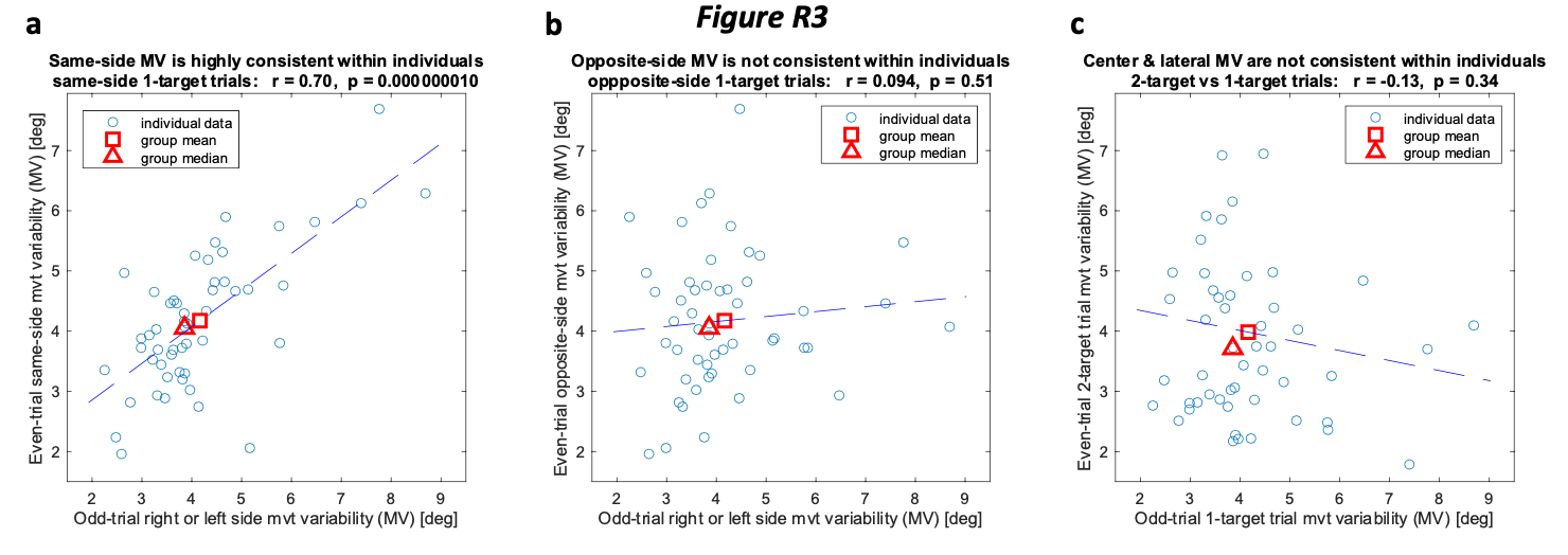
Analysis of left-side vs right-side 1-target trial data indicates the existence of participant-specific spatial patterns of variability.
With the participant-averaged data showing almost identical levels of motor variability on 1-target and 2-target trials, it is not surprising that about half of participants showed nominally greater variability on 1-target trials and about half showed nominally greater variability on 2-target trials. What was somewhat surprising, however, was that 16 of the 26 individual participants in Expt 2b displayed significantly higher variability in one condition or the other at α=0.05 (and 12/26 at α=0.01). Why might this be the case? We found an analogous result when breaking down the 1-target trial data into +30° (right-target) and -30° (left-target) trials that could offer an explanation. Note that the 2-target trial data come from intermediate movements toward the middle of the workspace, whereas the 1-target trial data come from right-side or left-side movements that are directed even more laterally than the +30° or -30° targets themselves (the average movement directions to these obstacle-obstructed lateral targets were +52.8° and -49.0°, respectively, in the Expt 2b data, see Fig 4a in the main paper for an illustration). Given the large separation between 1 & 2-target trials (~50°) and between left and right 1-target trails (~100°), differences in motor variability would not be surprising. The analyses illustrated in Figs R3-R6 show that these spatial differences indeed have large intra-individual effects on movement variability (Fig R3) and, critically, large a subsequent effect on the ability to predict the safety margin observed in one movement direction from motor variability observed at another (Figs R4-R6).
Fig R3 shows evidence for intra-individual direction-dependent differences in motor variability, obtained by looking at the similarity between within-participant spatially-matched (e.g. left vs left or right vs right, Fig R3a) compared to spatially-mismatched (left vs right, Fig R3b) motor variability across individuals. To perform this analysis fairly, we separated the 60 left-side obstacle1-target trial movements for each participant into those from odd-numbered vs even-numbered trials (30 each) to be compared. And we did the same thing for the 60 right-side obstacle 1-target trial movements. Fig R3a shows that there is a large (r=+0.70) and highly significant (p<10-6) across-participant correlation between the variability measured in the spatially-matched case, i.e. for the even vs odd trials from same-side movements, indicating that the measurement noise for measuring movement variability using n=30 movements (movement variability was measured by standard deviation) did not overwhelm inter-individual differences in movement variability.
The strength of this correlation would increase/decrease if we had more/less data from each individual because that would decrease/increase the noise in measuring each individual’s variability. Therefore, to be fair, we maintained the same number of data points for each variability measurement (n=30) for the spatially-mismatched cases shown in Fig R3b and R3c. The strong positive relationship between odd-trial and even-trial variability across individuals that we observed in the spatially-matched case is completely obscured when the target direction is not controlled for (i.e. not maintained) within participants, even though left-target and right-target movements are randomly interspersed. In particular, Fig R3b shows that there remains only a small (r=+0.09) and non-significant (p>0.5) across-participant correlation between the variability measured for the even vs odd trials from opposite-side movements that have movement directions separated by ~100°. This indicates that idiosyncratic intra-individual spatial differences in motor variability are large and can even outweigh inter-individual differences in motor variability seen in Fig R3a. Fig R3c shows that an analogous effect holds between the laterally-directed 1-target trials and the more center-directed 2-target trials that have movement directions separated by ~50°. In this case, the correlation that remains when the target direction is not is maintained within participants, is also near zero (r=-0.13) and non-significant (p>0.3). It is possible that some other difference between 1-target & 2-target trials might also be at play here, but there is unlikely to be a meaningful effect from decision variability given the essentially equal group-average variability levels (Fig R2).
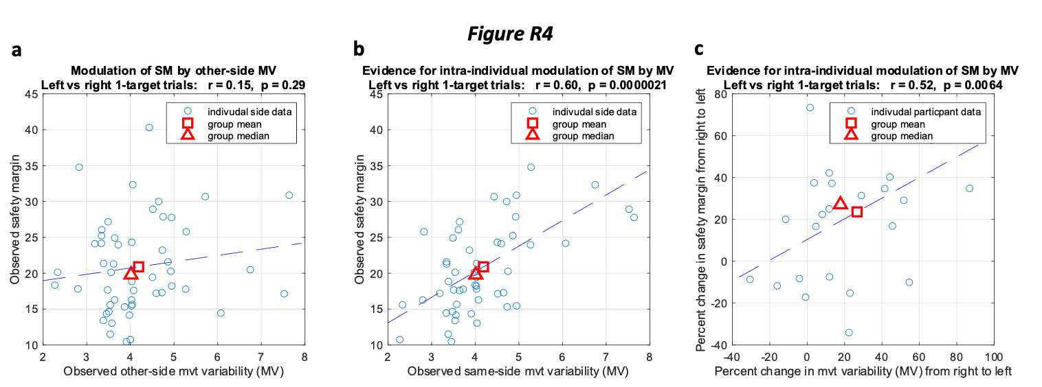
Analysis of left-side vs right-side 1-target trial data indicates that participant-specific spatial patterns of variability correspond to participant-specific spatial differences in safety margins.
Critically, dissection of the 1-target trial data also shows that the direction-dependent differences in motor variability discussed above for right-side vs left-side movements predict direction-dependent differences in the safety margins. In particular, comparison of panels a & b in Fig R4 shows that motor variability, if measured on the same side (e.g. the right-side motor variability for the right-side safety margin), strongly predicts interindividual differences in safety margin (r=0.60, p<0.00001, see Fig R4b). However, motor variability, if measured on the other side (e.g. the right-side motor variability for the left-side safety margin), fails to predict interindividual differences in safety margin (r=0.15, p=0.29, see Fig R4a). These data show that taking the direction-specific motor variability into account, allows considerably more accurate individual predictions of the safety margins used for these movements. In line with that idea, we also find that interindividual differences in the % difference between the motor variability measured on the left-side vs the right-side predicts inter-individual differences in the % difference between the safety margin measured on the left-side vs the right-side as shown in Fig R4c (r=0.52, p=0.006).
Analyses of both 1-target trial and 2-target trial data indicate that participant-specific spatial patterns of variability correspond to participant-specific spatial differences in safety margins.
Not surprisingly, the spatial/directional specificity of the ability to predict safety margins from measurements of motor variability observed in the 1-target trial data in Fig R4, is present in the 2-target data as well. Comparison of panels a-d in Fig R5 shows that motor variability from 1-target and 2-target trial data in Expt 2b strongly predict interindividual differences in 1-target and 2-target trial safety margins (r=0.72, p=3x10⁻⁵ for the 2-target trial data (see Fig R5d), r=0.59, p=1x10⁻³ for the 1-target trial data (see Fig R5a)).
This is the case even though the 1-target and 2-target trial data display essentially equal population-averaged levels of motor variability. However, in Expt 2b, motor variability, if measured on 1-target trials fails to predict inter-individual differences in the safety margin on 2-target trials (r=0.18, p=0.39, see Fig R5c), and motor variability, if measured on 2 target trials fails to predict inter-individual differences in the safety margin on 1-target trials (r=-0.12, p=0.55, see Fig R5b). As an aside, note that Fig 5a is similar to 4b in content, in that 1-target trial safety margins are plotted against motor variability levels in both cases. But in 5a, the left and right- target data are averaged whereas in 4b the left and right-target data are both plotted resulting in 2N data points. Also note that the correlations are similar, r=+0.59 vs r=+0.60, indicating that in both cases the amount of motor variability predicts the size of the safety margin.
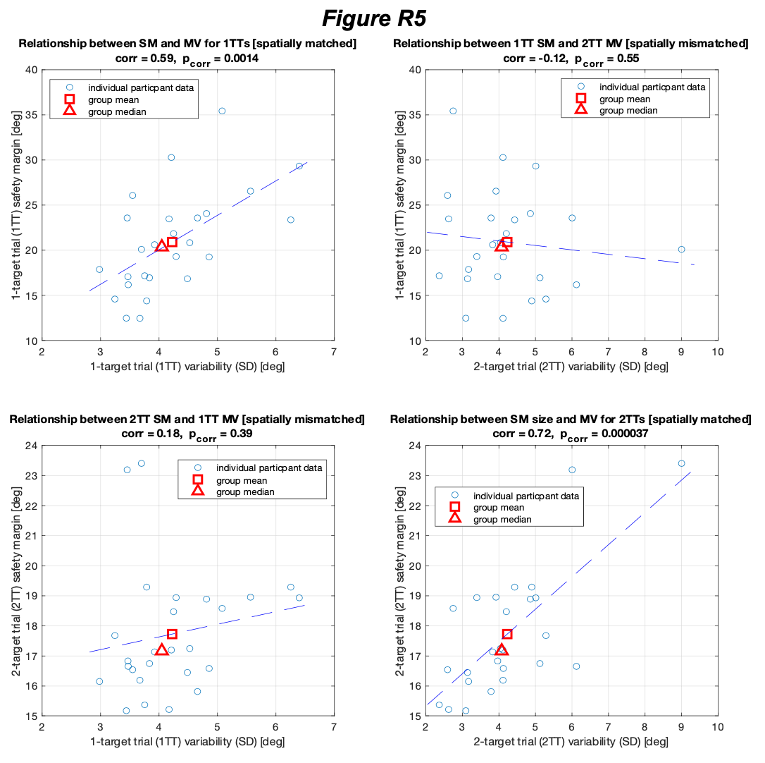
A final analysis indicating that the spatial specificity of motor variability rather than the presence of decision variability accounts for the ability to predict safety margins is shown in Fig R6. This analysis makes use of the contrast between Expt 2b (where there is a wide spatial separation (51° on average) between 1-target trials and 2-target trials because participants steer laterally around the Expt 2b 1-target trial obstacles, i.e. away from the center), and Expt 2a (where there is only a narrow spatial separation (10.4° on average) between the movement directions of 1-target trials and 2-target trials because participants steer medially around the Expt 2a 1-target trial obstacles, i.e. toward the center). If the spatial specificity of motor variability drove the ability to predict safety margins (and thus movement direction) on 2-target trials, then such predictions should be noticeably improved in Expt 2a compared to Expt 2b, because the spatial match between 1-target trials and 2-target trials is five-fold better in Expt 2a than in Expt2b. Fig R6 shows that this is indeed the case. Specifically, comparison of the 3rd and 4th clusters of bars (i.e. the data on the right side of the plot), shows that the ability to predict 2-target trial safety margins from 1-target trial variability and conversely the ability to predict 1-target trial safety margins from 2-target trial variability are both substantially improved in Expt 2a compared to Expt 2b (compare the grey bars in the 4th vs the 3rd clusters of bars).
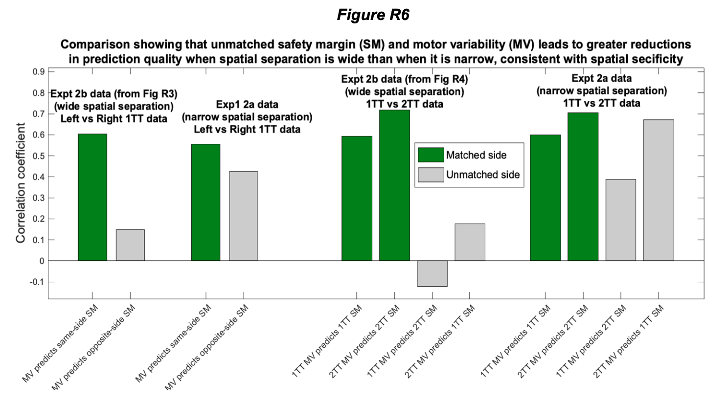
Moreover, comparison of the 1st and 2nd clusters of bars (i.e. the data on the left side of the plot), shows that the ability to predict left 1-target trial safety margins from right 1-target trial variability and conversely the ability to predict right 1-target trial safety margins from left 1-target trial variability are also both substantially improved in Expt 2a compared to Expt 2b (compare the grey bars in the 1st vs the 2nd clusters of bars). This corresponds to a spatial separation between the movement directions on left vs right 1-target trials of 20.7° on average in Expt 2a in contrast to a much greater 102° in Expt 2b.
The analyses illustrated in Figs R4-R6 make it clear that accurate prediction of interindividual differences in safety margins critically depend on spatially-specific information about motor variability, and we have, therefore, included this information for the analyses in the main paper, as it is especially important for the analysis of inter-individual differences in motor planning presented in Fig 5 of the manuscript.
3) Equation 3 then becomes even more involved and I believe it constitutes somewhat of a distractions from the main story - namely that individual variations in the safety margin in the 1-target obstacle-obstructed movements should lead to opposite correlations under the PO and MA hypotheses with the safety margin observed in the uncertain 2-target movements (see Fig 5e). Given that the logic of the variance-correction factor (pt 2) remains shaky to me, these analyses seem to be quite removed from the main question and of minor interest to the main paper.
The reviewer makes a good point. We agree that the original presentation made Equation 3 seem overly complex and possibly like a distraction as well. Based on the comment above and a number of comments and suggestions from Reviewer 2, we have now overhauled this content – streamlining it and making it clearer, in both motivation and presentation. Please see section 2.2 in the point-by-point response to reviewer 2 for details.
Reviewer #2:
The authors should be commended on the sharing of their data, the extensive experimental work, the experimental design that allows them to get opposite predictions for both hypotheses, and the detailed of analyses of their results. Yet, the interpretation of the results should be more cautious as some aspects of the experimental design offer some limitations. A thorough sensitivity analysis is missing from experiment 2 as the safety margin seems to be critical to distinguish between both hypotheses. Finally, the readability of the paper could also be improved by limiting the use of abbreviations and motivate some of the analyses further.
We thank the reviewer for the kind words and for their help with this manuscript.
1) The text is difficult to read. This is partially due to the fact that the authors used many abbreviations (MA, PO, IMD). I would get rid of those as much as possible. Sometimes, having informative labels could also help FFcentral and FFlateral would be better than FFA and FFB.
We have reduced the number of abbreviations used in the paper from 11 to 4 (Expt, FF, MA, PO), and we thank the reviewer for the nice suggestion about changing FFA and FFB to FFLATERAL and FFCENTER. We agree that the suggested terms are more informative and have incorporated them.
2) The most difficult section to follow is the one at the end of the result sections where Fig.5 is discussed. This section consists of a series of complicated analyses that are weakly motivated and explained. This section (starting on line 506) appears important to me but is extremely difficult to follow. I believe that it is important as it shows that, at the individual level, PO is also superior to MA to predict the behavior but it is poorly written and even the corresponding panels are difficult to understand as points are superimposed on each other (5b and e). In this section, the authors mention correcting for Mu1b and correcting for Sig2i/Sig1Ai but I don't know what such correction means. Furthermore, the authors used some further analyses (Eq. 3 and 4) without providing any graphical support to follow their arguments. The link between these two equations is also unclear. Why did the authors used these equations on the pooled datasets from 2a and 2b ? Is this really valid ? It is also unclear why Mu1Ai can be written as the product of R1Ai and Sig1Ai. Where does this come from ?
We agree with the reviewer that this analysis is important, and the previous explanation was not nearly as clear as it could have been. To address this, we have now overhauled the specifics of the context in Figure 5 and the corresponding text – streamlining the text and making it clearer, in both motivation and presentation (see lines 473-545 in the revised manuscript). In addition to the improved text, we have clarified and improved the equations presented for analysis of the ability of the performance optimization (PO) model to explain inter-individual differences in motor planning in uncertain conditions (i.e. on 2-target trials) and have provided more direct graphical support for them. Eq 4 from the original manuscript has been removed, and instead we have expanded our analyses on what was previously Eq 3 (now Eq 5 in the revised manuscript). We have more clearly introduced this equation as a hybrid between using group-averaged predictions and participant-individualized predictions, where the degree of individualization for all parameters is specified with the individuation index 𝑘. For example, a value of 1 for 𝑘 would indicate complete weighting of the individuated model predictors. The equation that follows in the revised manuscript, Eq 6, is a straightforward extension of Eq 5 where each model parameter was instead multiplied by a different individuation index. With this, we now present the partial-R2 statistic associated with each model predictor (see revised Figs 5a and 5e) to elucidate the effect of each. We have, additionally, now plotted the relationships between the each of the 3 model predictors and the inter-individual differences that remain when the other two predictors are controlled (see revised Figs 5b-d and Fig 5f-h). These analyses are all shown separately for each experiment, as per the reviewer’s suggestion, in the revised version of Fig 5.
Overall, this section is now motivated and discussed in a more straightforward manner, and now provides better graphical support for the analyses reported in the manuscript. We feel that the revised analysis and presentation (1) more clearly shows the extent to which inter-individual differences in motor planning can be explained by the PO model, and (2) does a better job of breaking down how the individual factors in the model contribute to this. We sincerely thank the reviewer for helping us to make the paper easier to follow and better illustrated here.
3) In experiment 1, does the presence of a central target not cue the participants to plan a first movement towards the center while such a central target was never present in other motor averaging experiment.
Unfortunately, the reviewer is mistaken here, as central target locations were present in several other experiments that advocated for motor averaging which we cite in the paper. The central target was not present on any 2-target trials in our experiments, in line with previous work. It was only present on 1-target center-target trials.
In the adaptation domain, people complain that asking where people are aiming would induce a larger explicit component. Similarly, one could wonder whether training the participants to a middle target would not induce a bias towards that target under uncertainty.
Any “bias” of motor output towards the center target would predict an intermediate motor output which would favor neither model because our experiment designs result in predictions for motor output on different sides of center for 2-target trials in both Expt 1 and Expt 2b. Thus we think any such effect, if it were to occur, would simply reduce the amplitude of the result. However, we found an approximately full-sized effect, suggesting that this is not a key issue.
4) The predictions linked to experiment 2 are highly dependent on the amount of safety margin that is considered. While the authors mention these limitations in their paper, I think that it is not presented with enough details. For instance, I would like to see a figure similar to Fig.4B when the safety margin is varied.
We apologize for any confusion here. The reviewer seems to be under the impression that we can specifically manipulate safety margins around the obstacle in making model predictions for experiment 2. This is, however, not the case for either of the two safety margins in the performance-optimization (PO) modelling. Let us clarify. First, the safety margin on 1-target trials, which serves as input to the PO model, is experimentally measured on obstacle-present 1-target trials, and thus cannot be manipulated. Second, the predicted safety margin on 2-target trials is the output of the PO model and thus cannot be manipulated. There is only one parameter in the main PO model (the one for making the PO prediction for the group-average data presented in Fig 4b, see Eq 4), and that is the motor cost weighting coefficient (𝛽). 𝛽 is implicitly present in Eq 2 as well, fixed at 1/2 in this baseline version of the PO model. It is of course true that changing the motor cost weighting will affect the model output (the predicted 2-trial safety margin), but we do not think that the reviewer is referring to that here, since he or she asks about that directly in section 2.4.4 and in section 2.4.6 below, where we provide the additional analysis requested.
For exp1, it would be good to demonstrate that, even when varying the weight of the two one-target profiles for motor averaging, one never gets a prediction that is close to what is observed.
Here the reviewer is referring an apparent inconsistency between our analysis of Expts 1 and 2, because in Expt 2 (but not in Expt 1) we examine the effect of varying the relative weight of the two 1-target trials for motor averaging. However, we only withheld this analysis in Expt 1 because it would have little effect. Unlike Expt 2, the measured motor output on left and right 1-target trials in Expt 1 is remarkably similar (see the left panel in Fig R7a below (which is based on Fig 2b from the manuscript)). This is because left and right 1-target trials in Expt 1 were adapted to the same FF perturbation ( FFLATERAL in both cases), whereas left and right 1-target trials in Expt 2 received very different perturbation levels, because one of these targets was obstacle-obstructed and the other was not. Therefore, varying the relative weightings in Expt 1 would have little effect on the MA prediction as shown in Fig R7b at right. We now realize that is point was not explained to readers, and we have now modified the text in the results section where the analysis of Expt 1 is discussed in order to include a summary of the explanation offered above. We thank the reviewer for surfacing this.
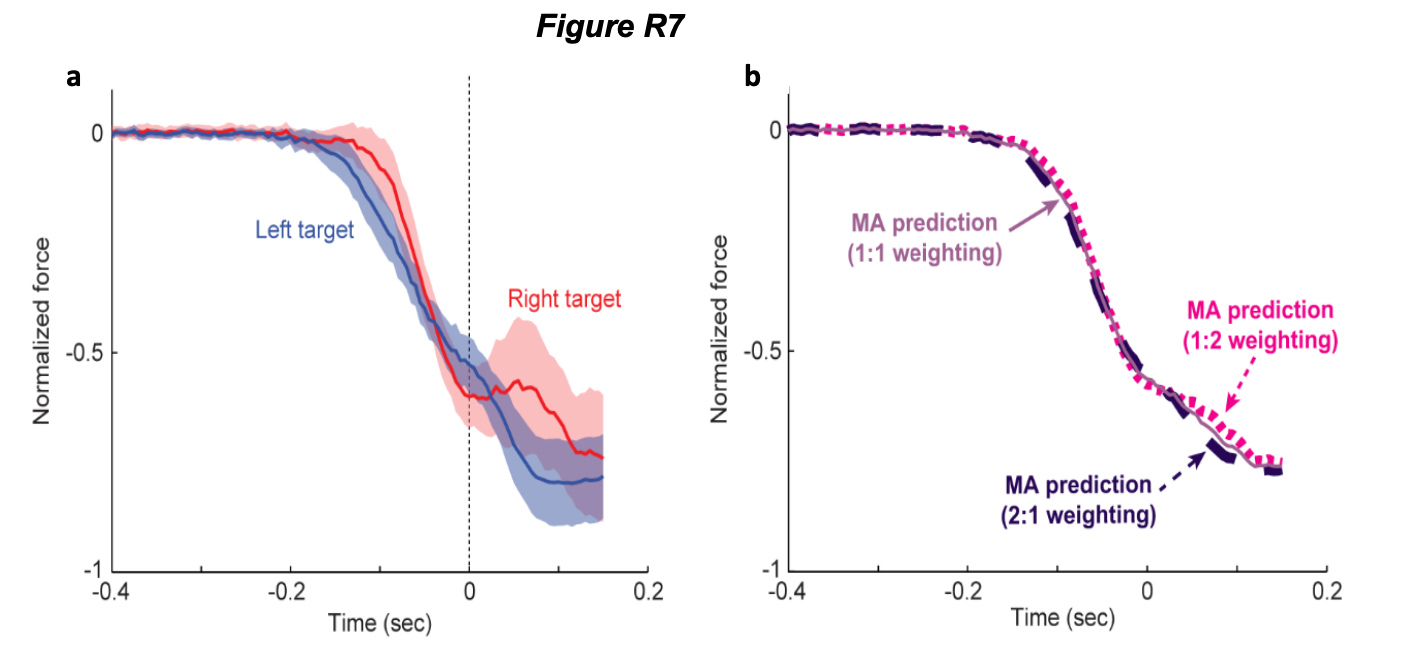
It is unclear in the text that the performance optimization prediction simply consists of the force-profile for the center target. The authors should motivate this choice.
We’re a bit unclear about this comment. This specific point is addressed in the first paragraph under the Results section, the second paragraph under the subsection titled “Adaptation to novel physical dynamics can elucidate the mechanisms for motor planning under uncertainty”, the Figure 2 captions, and in the second paragraph under the subsection titled “Adaptation to a multi-FF environment reveals that motor planning during uncertainty occurs via performance-optimization rather than motor averaging”. Direct quotes from the original manuscript are below:
Line 143: “However, PO predicts that these intermediate movements should be planned so that they travel towards the midpoint of the potential targets in order to maximize the probability of final target acquisition. This would, in contrast to MA, predict that intermediate movements incorporate the learned adaptive response to FFB, appropriate for center-directed movements, allowing us to decisively dissociate PO from MA.”
Line 200: “In contrast, PO would predict that participants produce the force pattern (FFB) appropriate for optimizing the planned intermediate movement since this movement maximizes the probability of successful target acquisition5,34 (Fig 1d, right).”
Line 274: “The 2-target trial MA prediction corresponds to the average of the force profiles (adaptive responses) associated with the left and right 1-target EC trials plotted in Fig 2b, whereas the 2-target trial PO prediction corresponds to the force profile associated with the center target plotted in Fig 2b, as this is appropriate for optimizing a planned intermediate movement.”
For the second experiment 2, the authors do not present a systematic sensitivity analysis. Fig. 5a and d is a good first step but they should also fit the data on exp2b and see how this could explain the behavior in exp 2a. Second, the authors should present the results of the sensitivity analysis like they did for the main predictions in Fig.4b.
We thank the reviewer for these suggestions. We have now included a more-complete analysis in Fig R8 below, and presented it in the format of Fig 4b as suggested. Please note that we have included the analysis requested above in a revised version of Fig 4b in the manuscript, and ta related analysis requested in section 2.4.6 in the supplementary materials.
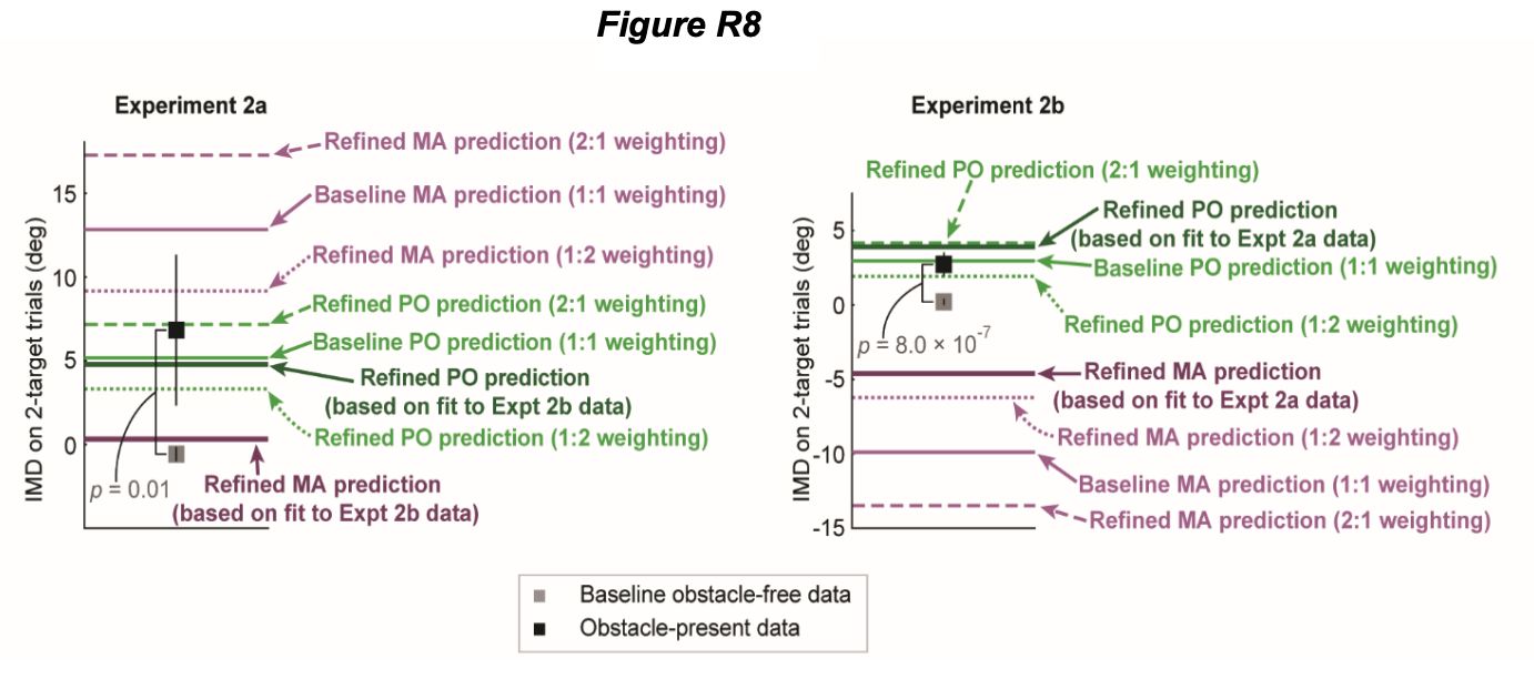
Specifically, the partial version of the analysis that had been presented (where the cost weighting for PO as well as the target weighting for MA were fit on Expt 2a and cross-validated using the Expt 2b data, but not conversely fit on Expt 2b and tested on Expt 2a) was expanded to include cross-validation of the Expt 2b fit using the Expt 2a data. As expected, the results from the converse analysis (Expt2b à Expt2a) mirror the results from the original analysis (Expt 2a à Expt 2b) for the cost weighting in the PO model, where the self-fit mean squared prediction errors modestly by 11% for the Expt 2a data, and by 29% for the Expt 2b data. In contrast, for the target weighting in the MA model, the cross-validated predictions did not explain the data well, increasing the self-fit mean squared prediction errors by 115% for the Expt 2a data, and by 750% for the Expt 2b data. Please see lines 411-470 in the main paper for a full analysis.
While I understand where the computation of the safety margin in eq.2 comes from, reducing the safety margin would make the predictions linked to the performance optimization look more and more towards the motor averaging predictions. How bad becomes the fit of the data then ?
We think that this is essentially the same question as that asked in above in section 2.4.1. Please see our response in that section above. If that response doesn’t adequately answer this question, please let us know!
How does the predictions look like if the motor costs are unbalanced (66 vs. 33%, 50 vs. 50% (current prediction), 33 vs. 66% ). What if, in Eq.2 the slope of the relationship was twice larger, twice smaller, etc.
Fig R8 above shows how PO prediction would change using the 2:1 (66:33) and 1:2 (33:66) weightings suggested by the reviewer here, in comparison to the 1:1 weighting present in the original manuscript, the Expt 2a best fit weighting present in the original manuscript, and the Expt 2b best fit weighting that the reviewer suggested we include in section 2.4.2. Please note that this figure is now included as a supplementary figure to accompany the revised manuscript.
The safety margin is the crucial element here. If it gets smaller and smaller, the PO prediction would look more and more like the MA predictions. This needs to be discussed in details. I also have the impression that the safety margin measured in exp 2a (single target trials) could be used for the PO predictions as they are both on the right side of the obstacle.
We again apologize for the confusion. We are already using safety margin measurements to make PO predictions. Specifically, within Expt 2a, we use safety margin measurements from 1-target trials (in conjunction with variability measurements on 1 & 2 target trials) to estimate safety margins on 2-target trials. And analogously within Expt 2b, we use safety margin measurements from 1-target trials (in conjunction with variability measurements on 1 & 2 target trials) to estimate safety margins on 2-target trials. Fig 4b in the main paper shows the results of this prediction (and it now also includes the cross-validated predictions of the refined models as requested in Section 2.4.4 above. Relatedly Fig R1 in this letter shows that, at the group-average level, these predictions for 2-target trial behavior in both Expt 2a and Expt 2b are essentially identical whether they are based solely on the safety margins observed on 1-target trials or on these safety margins corrected for the relative motor variabilities on 1-target and 2-target trials.
5) On several occasions (e.g. line 131), the authors mention that their result prove that humans form a single motor plan. They don't have any evidence for this specific aspect as they can only see the plan that is expressed. They can prove that the latter is linked to performance optimization and not to the motor averaging one. But the absence of motor averaging does not preclude the existence of other motor plans…. Line 325 is the right interpretation.
Thanks for catching this. We agree and have now revised the text accordingly (see for example, lines 53, 134, and 693-695 in the revised manuscript).
6) Line 228: the authors mention that there is no difference in adaptation between training and test periods but this does not seem to be true for the central target. How does that affect the interpretation of the 2-target trials data ? Would that explain the remaining small discrepancy between the refined PO prediction and the data (Fig.2f) ?
There must be some confusion here. The adaptation levels in the training period and the test period data from the central target are indeed quite similar, with only a <10% nominal difference in adaptation between them that is not close to statistically significant (p=0.14). We also found similar adaptation levels between the training and test epochs for the lateral targets (p=0.65 for the left target and p=0.20 for the right target). We further note that the PO predictions are based on test period data. And so, even if there were a clear decrease in adaptation between training and test periods, it would not affect the fidelity of the predictions or present a problem, except in the extreme hypothetical case where the reduction was so great that the test period adaptation was not clearly different from zero (as that would infringe on the ability of the paradigm to make clearly opposite predications for the MA and PO model) – but that is certainly not the case in our data.
Reviewer #3:
In this study, Alhussein and Smith provide two strong tests of competing hypotheses about motor planning under uncertainty: Averaging of multiple alternative plans (MA) versus optimization of motor performance (PO). In this first study, they used a force field adaptation paradigm to test this question, asking if observed intermediate movements between competing reach goals reflected the average of adapted plans to each goal, or a deliberate plan toward the middle direction. In the second experiment, they tested an obstacle avoidance task, asking if obstacle avoidance behaviors were averaged with respect to movements to non-obstructed targets, or modulated to afford optimal intermediate movements based on a commuted "safety margin." In both experiments the authors observed data consistent with the PO hypothesis, and contradictory of the MA hypothesis. The authors thus conclude that MA is not a feasible hypothesis concerning motor planning under uncertainty; rather, people appear to generate a single plan that is optimized for the task at hand.
I am of two minds about this (very nice) study. On the one hand, I think it is probably the most elegant examination of the MA idea to date, and presents perhaps the strongest behavioral evidence (within a single study) against it. The methods are sound, the analysis is rigorous, and it is clearly written/presented. Moreover, it seems to stress-test the PO idea more than previous work. On the other hand, it is hard for me to see a high degree of novelty here, given recent studies on the same topic (e.g. Haith et al., 2015; Wong & Haith, 2017; Dekleva et al., 2018). That is, I think these would be more novel findings if the motor-averaging concept had not been very recently "wounded" multiple times.
We thank the reviewer for the kind words and for their help with this manuscript.
The authors dutifully cite these papers, and offer the following reasons that one of those particular studies fell short (I acknowledge that there may be other reasons that are not as explicitly stated): On line 628, it is argued that Wong & Haith (2017) allowed for across-condition (i.e., timing/spacing constraints) strategic adjustments, such as guessing the cued target location at the start of the trial. It is then stated that, "While this would indeed improve performance and could therefore be considered a type of performance-optimization, such strategic decision making does not provide information about the implicit neural processing involved in programming the motor output for the intermediate movements that are normally planned under uncertain conditions." I'm not quite sure the current paper does this either? For example, in Exp 1, if people deliberately strategize to simply plan towards the middle on 2-target trials and feedback-correct after the cue is revealed (there is no clear evidence against them doing this), what do the results necessarily say about "implicit neural processing?" If I deliberately plan to the intermediate direction, is it surprising that my responses would inherit the implicit FF adaption responses from the associated intermediate learning trials, especially in light of evidence for movement- and/or plan-based representations in motor adaptation (Castro et al., 2011; Hirashima & Nozacki, 2012; Day et al., 2016; Sheahan et a., 2016)?
The reviewer has a completely fair point here, and we agree that the experiments in the current study are amenable to explicit strategization. Thus, without further work, we cannot claim that the current results are exclusively driven by implicit neural processing.
As the reviewer alludes to below, the possibility that the current results are driven by explicit processes in addition to or instead of implicit ones does not directly impact any of the analyses we present – or the general finding that performance-optimization, not motor averaging, underlies motor planning during uncertainty. Nonetheless, we have added a section in the discussion section to acknowledge this limitation. Furthermore, we highlight previous work demonstrating that restriction of movement preparation time suppresses explicit strategization (as the reviewer hints at below), and we suggest leveraging this finding in future work to investigate how motor output during goal uncertainty might be influenced under such constraints. This portion of the discussion section is quoted below:
“An important consideration for the present results is that sensorimotor control engages both implicit and explicit adaptive processes to generate motor output47. Because motor output reflects combined contributions of these processes, determining their individual contributions can be difficult. In particular, the experiments in the present study used environmental perturbations to induce adaptive changes in motor output, but these changes may have been partially driven by explicit strategies, and thus the extent to which the motor output measured on 2-target trials reflects implicit vs explicit feedforward motor planning requires further investigation. One method for examining implicit motor planning during goal uncertainty might take inspiration from recent work showing that in visuomotor rotation tasks, restricting the amount of time available to prepare a movement appears to limit explicit strategization from contributing to the motor response48–51. Future work could dissociate the effects of MA and PO on intermediate movements in uncertain conditions at movement preparation times short enough to isolate implicit motor planning.”
In that same vein, the Gallivan et al 2017 study is cited as evidence that intermediate movements are by nature implicit. First, it seems that this consideration would be necessarily task/design-dependent. Second, that original assumption rests on the idea that a 30˚ gradual visuomotor rotation would never reach explicit awareness or alter deliberate planning, an assumption which I'm not convinced is solid.
We generally agree with the reviewer here. We might add that in addition to introducing the perturbation gradually, Gallivan and colleagues enforced a short movement preparation time (325ms). However, we agree that the extent to which explicit strategies contribute to motor output should clearly vary from one motor task to another, and on this basis alone, the Gallivan et al 2017 study should not be cited as evidence that intermediate movements must universally reflect implicit motor planning. We have explained this limitation in the discussion section (see quote below) and have revised the manuscript accordingly.
“We note that Gallivan et al. 2017 attempted to control for the effects of explicit strategies by (1) applying the perturbation gradually, so that it might escape conscious awareness, and (2) enforcing a 325ms preparation time. Intermediate movements persisted under these conditions, suggesting that intermediate movements during goal uncertainty may indeed be driven by implicit processes. However, it is difficult to be certain whether explicit strategy use was, in fact, effectively suppressed, as the study did not assess whether participants were indeed unaware of the perturbation, and the preparation times used were considerably larger than the 222ms threshold shown to effectively eliminate explicit contributions to motor output."
The Haith et al., 2015 study does not receive the same attention as the 2017 study, though I imagine the critique would be similar. However, that study uses unpredictable target jumps and short preparation times which, in theory, should limit explicit planning while also getting at uncertainty. I think the authors could describe further reasons that that paper does not convince them about a PO mechanism.
We had omitted a detailed discussion of the Haith et al 2015 study as we think that the key findings, while interesting, have little to do with motor planning under uncertainty. But we now realize that we owe readers an explanation of our thoughts about it, which we have now included in the Discussion. This paragraph is quoted below, and we believe it provides a compelling reason why the Haith et al. 2015 study could be more convincing about PO for motor planning during uncertainty.
“Haith and colleagues (2015) examined motor planning under uncertainty using a timed-response reaching task where the target suddenly shifted on a fraction (30%) of trials 150-550ms] before movement initiation. The authors observed intermediate movements when the target shift was modest (±45°), but direct movements towards either the original or shifted target position when the shift was large (±135°). The authors argued that because intermediate movements were not observed under conditions in which they would impair task performance, that motor planning under uncertainty generally reflects performance-optimization. This interpretation is somewhat problematic, however. In this task, like in the current study, the goal location was uncertain when initially presented; however, the final target was presented far enough before movement onset that this uncertainty was no longer present during the movement itself, as evidenced by the direct-to-target motion observed when the target location was shifted by ±135°. Therefore the intermediate movements observed when the target location shifted by ±45° are unlikely to reflect motor planning under uncertain conditions. Instead, these intermediate movements likely arose from a motor decision to supplement the plan elicited by the initial target presentation with a corrective augmentation when the plan for this augmentation was certain. The results thus provide beautiful evidence for the ability of the motor system to flexibly modulate the correction of existing motor plans, ranging from complete inhibition to conservative augmentation, when new information becomes available, but provide little information about the mechanisms for motor planning under uncertain conditions.”
If the participants in Exp 2 were asked both "did you switch which side of the obstacle you went around" and "why did you do that [if yes to question 1]", what do the authors suppose they would say? It's possible that they would typically be aware of their decision to alter their plan (i.e., swoop around the other way) to optimize success. This is of course an empirical question. If true, it wouldn't hurt the authors' analysis in any way. However, I think it might de-tooth the complaint that e.g. the Wong & Haith study is too "explicit."
The participants in Expts 1, 2a, and 2b were all distinct, so there was no side-switching between experiments per se. However, the reviewer’s point is well taken. Although we didn’t survey participants, it’s hard to imagine that any were unaware of which side they traveled around the obstacle in Expt 2. Certainly, there was some level of awareness in our experiments, and while we would like to believe that the main findings arose from low-level, implicit motor planning, we frankly do not know the extent to which our findings may have depended on explicit planning. We have now clarified this key point and discussed it’s implications in the discussion section of the revised paper. That said, we do still think that the direct-to-target movements in the Wong and Haith study were likely the result of a strategic approach to salvaging some reward in their task. Please see the new section in the discussion titled: “Implicit and explicit contributions to motor planning under uncertainty” which for convenience is copied below:
Implicit and explicit contributions to motor planning under uncertainty An important consideration for the present results is that sensorimotor control engages both implicit and explicit adaptive processes to generate motor output. Because motor output reflects combined contributions of these processes, determining their individual contributions can be difficult. In particular, the experiments in the present study used environmental perturbations to induce adaptive changes in motor output, but these changes may have been partially driven by explicit strategies, and thus the extent to which the motor output measured on 2-target trials reflects implicit vs explicit feedforward motor planning requires further investigation. One method for examining implicit motor planning during goal uncertainty might take inspiration from recent work showing that in visuomotor rotation tasks, restricting the amount of time available to prepare a movement appears to limit explicit strategization from contributing to the motor response. Future work could dissociate the effects of MA and PO on intermediate movements in uncertain conditions at movement preparation times short enough to isolate implicit motor planning.
We note that Gallivan et al. 2017 attempted to control for the effects of explicit strategies by (1) applying the perturbation gradually, so that it might escape conscious awareness, and (2) enforcing a 325ms preparation time. Intermediate movements persisted under these conditions, suggesting that intermediate movements during goal uncertainty may indeed be driven by implicit processes. However, it is difficult to be certain whether explicit strategy use was, in fact, effectively suppressed, as the study did not assess whether participants were indeed unaware of the perturbation, and the preparation times used were considerably larger than the 222ms threshold shown to effectively eliminate explicit contributions to motor output.
Author Response:
Reviewer #3:
Weaknesses:
Previously it was suggested that mitochondrial biogenesis was increased with increased levels of GJA1-20k. Is this a difference in the cellular model (HEK) and do the changes in cell culture accurately recapitulate the changes seen in animals?
The Reviewer is correct that GJA1-20k did not alter the mitochondrial biogenesis in HEK293 cells (Figure 1–figure supplement 2) whereas AAV9-transduced adult cardiomyocytes showed increased mitochondrial DNA copy number (Figure 1–figure supplement 2C), consistent with our previous study (Basheer et al., JCI insight, 2018). We expect that increased mitochondrial biogenesis is a function of chronic GJA1-20k overexpression in vivo, and thus a separate phenomenon from the acute mitochondrial fission which occurs within one minute of GJA1-20k accumulation around a mitochondrion (Figure 4). The HEK cell line, in which overexpressed GJA1-20k is present for a much shorter time, does not induce mitochondrial biogenesis (Figure 1–figure supplement 2), and thus is an excellent cellular model in which we can study GJA1-20k induced fission.
The revised manuscript has been modified to include the above new data (Figure 1–figure supplement 2) and discussion:
—Results section (lines 121 – 129): Previously we reported that GJA1-20k is involved in mitochondrial biogenesis (Basheer, Fu et al. 2018). Consistent with our previous study, AAV9-transduced adult cardiomyocytes showed increased mitochondrial DNA copy number and GJA1-20k deficient mice (Gja1M213L/M213L) had decreased copy number. However, exogenous GJA1-20k did not alter the mitochondrial biogenesis in HEK293 cells. Nor did exogenous GJA1-20k affect membrane potential or baseline ATP production (Figure 1–figure supplement 2A–C). In addition to mitochondrial DNA copy number, neither biogenesis nor mitophagy protein markers were altered in either GJA1-20k transfected HEK293 cells or Gja1M213L/M213L mouse hearts (Figure 1–figure supplement 2D – G).
—Discussion section (lines 289 – 292): Yet the presence of GJA1-20k, while inducing mitochondrial fission and smaller mitochondria (Figure 1, 3 and 4), does not either reduce MFN1 or MFN2, activate DRP1, change membrane potential, ATP production, mitochondrial biogenesis, or mitophagy (Figure 2; Figure 1 – figure supplement 2).
Mdivi-1 is not a selective Drp1 inhibitor. It is a Complex I inhibitor, leading to unintended changes in mitochondrial dynamics in response to ETC stress. Rather than Mdivi-1, a dominant negative Drp1 mutant K38A could be overexpressed to see whether this prevents GJA1-20k-mediated fission. If it still goes through, then I agree that Drp1 is not involved at all.
We appreciate Reviewer #3’s thoughtful suggestion and, in this revised manuscript, we studied mitochondrial morphology in the presence of K38A. As seen in Figure 2C and D of the revised manuscript, K38A elongated mitochondria, as expected from inhibited Drp1 mediated fission. However, despite Drp1 inhibition by K38A, in the presence of GJA1-20k, mitochondria remain small, further supporting that GJA1-20k-mediated fission is DRP1-independent.
—Results section (lines 140 – 150): To further investigate whether GJA1-20k induced reduction in mitochondrial size is dependent on DRP1, we analyzed mitochondrial morphology after inhibiting DRP1 by performing siRNA- mediated DRP1 knock-down (Figure 2—figure supplement 1A–C) or transfecting DRP1 dominant negative mutant (K38A), all with or without GJA1-20k transfection. With either method of DRP1 inhibition, the average area of individual mitochondria increased, consistent with inhibiting canonical fission (Figure 2C, D). In addition, K38A has more pronounced DRP1 inhibition which resulted in greater mitochondrial enlargement than siDRP1 (Figure 2C, D; Figure 2—figure supplement 1F). However, GJA1-20k acts epistatically to DRP1 loss or interference and prevents DRP1-mediated mitochondrial enlargement (Figure 2C–F; Figure 2— figure supplement 1B, C), indicating GJA1-20k can act at or downstream of DRP1.
For the kinetics studies (see Fig 4), I think it is important to measure the timing of the actin recruitment and eventual fission when Drp1 is knocked down and/or when a DN mutant (K38A) is involved. Again, I do not trust the chemical inhibitor (Mdivi-1) data since this does not inhibit Drp1 activity.
We would like to thank Reviewer #3 for suggesting we use an additional method of inhibiting Drp1. We analyzed real time actin dynamics under direct DRP1 knock-down. As seen in Mdivi-1 treatment, GJA1- 20k accumulated and then actin assembled around mitochondria and induced fission under DRP1 knockdown (Figure 4 and Video 1 of revised manuscript). The kinetic parameters of fission were also similar between Drp1 knockdown and Mdivi-1 treatment. The original Figure 4 and Video 1 and 2 have been moved to Figure 4–figure supplement 1 and Video 2 and 3, respectively, in order to accommodate the new Drp1 knockdown data (Figure 4 and Video 1).
The revised manuscript has been modified to include the above new data (Figure 4; Video 1):
—Results section (lines 198 – 219): Simultaneous use of fluorescently labelled actin, GJA1-20k, and mitochondria in live cells permit real time imaging of mitochondrial fission events at actin assembly sites. As seen in Video 1 and Figure 4B, GJA1-20k recruits actin to mitochondria, which results in fission. In Video 1, the actin network can be seen to develop around mitochondria and, coinciding with GJA1-20k intensity, forms an increasingly tight band across a mitochondrion which, within one minute, results in mitochondrial fission. The imaging in the bottom row of Figure 4B, and in the right column of Video 1 were obtained by multiplying GJA1-20k signal with actin signal, highlighting the locations at which GJA1-20k and actin are coincident. The respective line-scan profiles in Figure 4C indicate that mitochondrial fission occurs at points where the product of GJA1-20k and actin is the highest. Following accumulation of GJA1-20k and actin (red lines) at these points, a drop in mitochondrial signal (blue lines) is apparent when fission occurs. Fission (low point of blue lines) occurs approximately 45 seconds after co-accumulation of GJA1-20k and actin (high point of red lines, Figure 4C). Time to fission was computed from the time of peak GJA1-20k and actin intensity product, to the time of mitochondrial signal being reduced to background (Figure 4D–F). Statistically, this time to fission occurred at a median of 45 seconds, with a standard deviation of 11 seconds (Figure 4G). Note, the real time imaging shown in Video 1, and Figure 4 were performed under siDRP1. Therefore, the mitochondrial fission induced by cooperation between GJA1-20k and actin can be independent of canonical DRP1-mediated fission. To rule out inadvertent bias by siRNA, we used pharmacologic Mdivi-1 to inhibit DRP1 and, similar to the use of DRP1 siRNA, actin formed around mitochondria at GJA1-20k sites (Figure 4—figure supplement 1A–D) and fission occurred within a similar timescale (Video 2 and 3; Figure 4— figure supplement 1E–H).
The assessment of the impact of ischemic stress with the heterozygous animal (M213L/WT) is hard to interpret. How reduced is the expression of GJA1-20k in these animals and how is mitochondrial function impacted based on Seahorse analysis? The mitochondrial morphology is not altered in these animals, so would mitochondrial function be largely unchanged as well? It is not clear how much GJA1-20k is needed to observe changes in mitochondrial shape and function, and comparisons with the homozygous mutant (M213L/M213L) are not the same, making it difficult to resolve the interpretation of these data.
We appreciate Reviewer #3’s thoughtful and valuable comments. We previously reported that the heterozygous mutant (M213L/WT) expresses approximately half of GJA1-20k compared to WT (Figure 1 in Xiao and Shimura et al., J Clin Invest, 2020). Unfortunately, homozygous mutants die before adulthood, preventing effective comparison of GJA1-20k content on mitochondrial function in adult cardiomyocytes. To compare the impact of the amount of endogenous GJA1-20k on mitochondrial function, we added seahorse data from heterozygous neonatal CMs (Figure 5 C, D) and compared these data to seahorse data from neonatal cardiomyocytes from both wildtype and homozygous mutants. Even though there was no significant difference in mitochondrial size between WT and M213L/WT (Figure 5I, J; Figure 5–figure supplement 1A, B) under basal conditions, the seahorse OCR levels from M213L/WT myocytes is in between that of WT and homozygous (M213L/M213L) (Figure 5 C, D; Figure 5–figure supplement 1C) cardiomyocytes. Since GJA1-20k is a stress responsive peptide which increases under ischemic stress, in the present manuscript, we should like to emphasize that even a partial (50%) decrease in GJA1-20k expression induces mitochondrial fragility to oxidative stress. As shown in new Figure 5 I – L of the revised manuscript, the heterozygous mutant (M213L/WT) has more elongated mitochondria and a high distribution of damaged mitochondria post-I/R compared to WT, consistent with TTC staining, even with no change in mitochondrial size under basal conditions.
The revised manuscript has been modified to include the above new data (Figure 5; Figure 5–figure supplement 1) and discussion:
—Results section (lines 227 – 233) Similarly, maximal respiration is increased in neonatal CMs derived from GJA1-20k deficient Gja1M213L/M213L mice and maximal respiration for heterozygous Gja1M213L/WT mice is between that of WT and Gja1M213L/M213L (Figure 5C, D; Figure 5—figure supplement 1A, B). In addition, observing other OCR parameters, we found a decrease in ATP-linked respiration and reserve capacity in Gja1M213L/WT cardiomyocytes, and an increase in proton leak and non-mitochondrial respiration in Gja1M213L/M213L suggesting that there can be compensatory long-term effects of the Gja1 mutation (Figure 5—figure supplement 1C).
—Results section (lines 241 – 250) However, remarkably, reduced GJA1-20k expression results in an almost complete cardiac infarction after I/R injury (Figure 5E, F). Moreover, ROS production after I/R injury was increased in Gja1M213L/WT mice compared to WT post-I/R (Figure 5G, H). There was no significant difference in mitochondria size at the basal condition between WT and Gja1M213L/WT mice adult CMs as with neonatal CMs (Figure 5I, J), whereas the mitochondria size was significantly increased after I/R injury and the heterozygous Gja1M213L/WT mice had larger mitochondria compared to WT mice post-I/R (Figure 5I, J). Interestingly, the area of mitochondrial matrix was also increased, suggesting loss of cristae in Gja1M213L/WT mice heart (Figure 5K, L). These data indicate that even partial deletion of GJA1-20k results in a profoundly impaired response to ischemic stress.
—Discussion section (lines 350 – 357) Because GJA1-20k-induced fission is associated with less ROS production with oxidative stress (Figure 5 – figure supplement 1D, E), the endogenous generation of GJA1-20k and subsequent decreased ROS production could explain a major benefit of pre-conditioning. Of note, genetic GJA1-20k reduction increases infarct size and ROS production post-I/R injury (Figure 5E–H). In addition, the population of damaged mitochondria is significantly increased in heterozygous Gja1M213L/WT mouse heart post-I/R (Figure 5I–L). Therefore, GJA1-20k induced decreases in ROS production could limit the amount of I/R injury induced by myocardial infarction.
It is still unclear to me how GJA1-20k is affecting mitochondrial size and function. Based on previous papers, this peptide localizes to the surface of mitochondria, but it is not clear how, or whether, it directly facilitates actin recruitment. The interplay with the endoplasmic reticulum (ER), which can nucleate actin at sites of mitochondrial fission, was not examined. If actin is driving membrane remodeling, is it mediated by ER crossover at these sites?
We appreciate Reviewer #3’s thoughtful comment and suggestion. Our unpublished data indicate that GJA1-20k has an actin-binding domain, suggesting direct binding and actin dynamics regulation. As shown in Figure 3 in the present study, GJA1-20k recruits actin around mitochondria membrane and their interaction resulted in fission. In addition, as the Reviewer suggested, our preliminary data showed significant increase in ER network in GJA1-20k-transfected cells (Figure below). Therefore, there is the possibility that ER is also involved in GJA1-20k mediated mitochondrial fission, while further research will be required to reveal the detailed mechanisms. In the present manuscript, we would like to focus on the finding that actin is necessary for GJA1-20k-mediated mitochondrial fission but not DRP1.
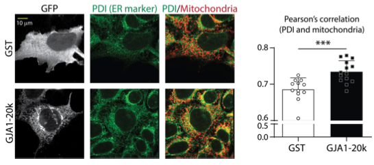
ER network association with mitochondria is increased in GJA1-20k-transfected cells. Left: Representative fixed cell images of HEK293 cells with GFP-tagged GST or GJA1-20k. ER and mitochondria were labeled by Protein disulfide-isomerase (PDI) and Tom20, respectively. Right: The quantification of Pearson’s correlation between PDI and mitochondria. The graph is expressed as mean ± SD. p values were determined by two-tailed Mann-Whitney U-test. ***p < 0.001.
We have updated the Discussion section to point to this excellent consideration in the future.
—Discussion section (lines 299 – 302) In addition to actin, the endoplasmic reticulum (ER) membrane can be involved in mitochondrial scission (Friedman, Lackner et al. 2011, Tandler, Hoppel et al. 2018). Future studies should be considered whether GJA1-20k induced actin cytoskeleton arrangements involves ER membrane as well.
Author Response
Reviewer #1 (Public Review):
The present study by Zander et al. aims at improving our understanding of CD4+ T cell heterogeneity in response to chronic viral infections. The authors utilize the murine LCMV c13 infection model and perform single cell RNA seq analysis on day 10 post infection to identify multiple, previously unappreciated, T cell subsets. The authors then go on and verify these analyses using multi-color flow cytometry before comparing the transcriptome of CD4 T cells from chronic infection to a previously generated data set of CD4 T cells obtained from acutely-resolved LCMV infection.
The analyses are very well done and provide some interesting novel insights. In particular, the comparison of CD4 T cell subsets across acute and chronic infections is very exciting as they provide a very valuable platform that can answer a long-standing question: do CD4 T cells in chronic infection undergo exhaustion similar to CD8 T cells. While this has been proposed for an extended period, this new dataset by Zander et al. can provide some novel insights by comparing individual cell subsets cross-infection. The manuscript would, however, benefit from a more extensive analysis and focus on this interesting point.
We thank the reviewer for their time and careful assessment of our manuscript. We were happy to hear that the reviewer found our work interesting.
On that note, the authors should take advantage of more accurate and present gene datasets to compare the 'dysfunctional' state of CD4 T cells in chronic infection vs acute infection. Also, a different illustration to demonstrate the module score analyses would be more intuitive.
We have now included T cell “exhaustion” genesets from recently published data (Zander et. al 2019 Immunity), and we have also displayed the relative expression of select signature genes from these genesets in an updated supplemental figure 3.
Also, at multiple sections in the manuscript, the authors are missing the accurate citations as they are still mentioned as '(Ref)'.
We apologize for this oversight and have corrected these citations.
Nevertheless, this study does not require major revisions.
Reviewer #2 (Public Review):
In their study "Delineating the transcriptional landscape and clonal diversity of virus-specific CD4+ T cells during chronic viral infection" Zander and co-workers analyze the phenotypic and clonotypic distributions of T cells specific to a LCMV epitope following infection with a chronic LCMV strain in mice. The paper largely follows an earlier study from the same group (Khatun JEM 2021) that has used a similar experimental strategy to analyze T cells responding to an LCMV strain establishing acute infection, and it adds a scTCRseq component to another earlier study of chronic LCMV (Zander Immunity 2022). The main contributions of the paper are to demonstrate that interesting differences between gene expression profiles between chronic and acute LCMV exist, and to identify a new T cell subset (of unknown functional significance).
While the paper is framed around differences between T cell responses to acute and chronic infections, all analysis is done on T cells at day 10 post primary infection. At such an early time point even the acute LCMV strain virus is likely not completely cleared, or at the very least viral antigens are still presented. The relevance of the presented phenotypic differences to other settings with long-term chronic infection is thus questionable. Additionally, there are a number of methodological concerns regarding the robustness of the statistical and bioinformatic analyses that put in doubt some of the conclusions. Most notably, the analysis of fate biases needs to be substantiated by tests against baseline expectations from random assortment to test for statistical significance.
We thank the reviewer for their careful review of our manuscript as well as their helpful comments.
Regarding the day 10 time point-post LCMV Armstrong infection, several groups have previously reported that LCMV viral load is undetectable by day 10 post-infection (see one published example below), although we completely agree with the reviewer that there is still likely to be viral antigens being presented at this time point, as well as ongoing inflammation, which we believe (and as discussed further below) is actually a strength of the study as it allows for a more fair comparison of the transcriptional state of recently stimulated virus-specific CD4 T cells under different contexts (acute vs chronic LCMV infection) . We chose day 10 post LCMV Cl13 and LCMV Armstrong infections as the timepoint for analysis, as this is approximately the peak of the endogenous Gp66-77 CD4+ T cell response (see previously published data below), and is also when there is a more balanced distribution of Th1, Tfh, and T central memory precursor (Tcmp)/ or memory-like cells in these settings, thereby allowing for sufficient numbers of cells/cluster to conduct an in-depth analysis and high-resolution comparison of these subsets between the two different infections. Further, as some degree of TCR stimulation is still likely being experienced at this timepoint during LCMV Armstrong infection, we believe that this is a more useful comparison than at a memory time point (when CD4 T cells are in a quiescent state) as it gives us a better picture of the differentially expressed genes at the peak of the CD4 T cell response, and also provides insight into how chronic viral infection perturbs the transcriptional program of CD4 T cells.
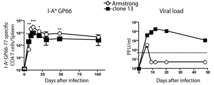
Author Response
Reviewer #4 (Public Review):
Francisco et al. investigate the role of CTP and hydrolysis in the binding of ParB to parS sequence and non-specific DNA at the single-molecule level. Using optical tweezers, they show the specific binding of ParB to parS sites, and demonstrate that this process is enhanced by the presence of CTP or CTPS. They find that lower density ParB proteins are also detected in distal non-specific DNA in the presence of parS, and that ParB spreading is restricted by protein roadblocks. Furthermore, using magnetic tweezers, they show that parS-containing DNA molecules are condensed by ParB at nanomolar protein concentration, which requires CTP binding but not hydrolysis. These finding show the significance of CTP-dependent ParB spreading and impact the understanding of the mechanism of DNA bridging and condensation by ParB networks.
Based on these results, the authors propose a model for ParB-mediated DNA condensation, which requires one-dimensional ParB sliding along DNA from parS sites. Overall, the experiments were carefully done and thoroughly controlled. The manuscript provides critical insights that can be strengthened by addressing the following minor concerns:
1) Did the authors observe the diffusion of isolated ParB foci along DNA? This will provide strong evidence for the proposed diffusion/sliding model.
2) Based on the sliding clamp model, ParB spreading and diffusion result in DNA condensation by forming large DNA loops. Is it possible to show the dynamic spreading of ParB while keep the same numbers of ParB on DNA? For example, can the authors incubate ParB-containing DNA in channel 4 (ParB channel) at a certain time for the loading of ParB on parS sites, and then move it to the buffer channel without free ParB as well as with CTP or CTPS, where the images are acquired at the long interval time to minimize the photobleaching. The fluorescent intensity of the ParB during the spreading process can be analyzed. If the intensity remains constant through spreading in the presence of CTPS but significantly decrease in the presence of CTP, this data will strongly demonstrate the proposed spreading and CTP hydrolysis-dependent dissociation mechanism.
We thank the reviewer for these suggestions to prove spreading. However, we decided to follow an alternative strategy based on the direct imaging of QD-labelled ParB. As described above, this strategy worked well and we have directly visualized ParB diffusion from parS sites.
3) In Figure 2, the authors show the spreading of ParB can be blocked by EcoRI. Can the authors show that EcoRI is bound at the specificity positions? The spreading blockage by protein roadblocks showed in optical tweezers experiments potentially hints that the roadblocks may affect the DNA condensation. Can the authors apply the magnetic tweezers to show the affection of protein roadblocks to DNA condensation in vitro?
It is well established that EcoRI has extremely high affinity and specificity for its site (Terry et al., 1983) and so, since we do not have labelled EcoRI mutant, our experiments assume the sites are occupied. This is one reason we have used multiple sites in our experiments. Nevertheless, we have tested the effect of protein roadblocks in condensation in MT experiments. We found partial concentration consistent with the blocking of spreading of ParB from parS (Fig. R5)
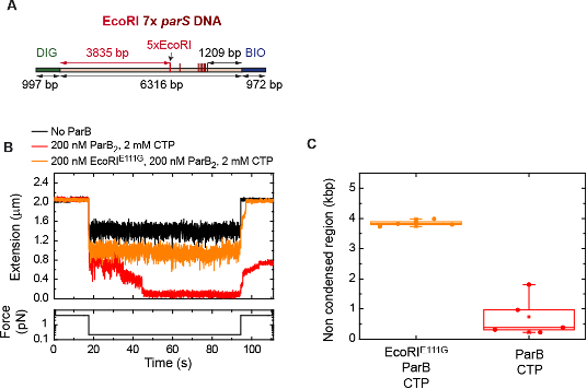
Figure R5. ParB diffusion is required for DNA condensation by ParB. (A) Schematic representation of DNA substrate employed in these MT experiments. It contains a set of 5x EcoRI sites located at 3835 bp from the DIG labelled end, and 7x parS. The positions of the EcoRI and parS sites in the DNA cartoon are represented to scale. (B) Condensation assay using the EcoRI 7x parS DNA substrate under different experimental conditions. ParB partially condenses the DNA molecule when EcoRIE111G is present. (C) Quantification of the extension in base pairs of the non-condensed region under different experimental conditions. In the presence of EcoRIE111G, the length of the non-condensed region agrees well with the length of the region flanked by the DIG end and the EcoRI sites.
Author Response
Reviewer #2 (Public Review):
This study evaluates the causal relationship between childhood obesity on the one hand, and childhood emotional and behavioral problems on the other. It applies Mendelian Randomization (MR), a family of methods in statistical genetics that uses genetic markers to break the symmetry between correlated traits, allowing inference of causation rather than mere correlation. The authors argue convincingly that previous studies of these traits, both those using non-genetic observational epidemiology methods and those using standard MR methods, may be confounded by demographic effects and familial effects. One possible example of this kind of confounding is that the idea that obesity in parents may contribute to emotional and behavioral problems in children; another is the idea that adults with emotional and behavioral issues may be more likely to have children with partners who are obese, and vice-versa. They then make use of a recently proposed "within-family" MR method, which should effectively control for these confounders, at the cost of higher uncertainty in the estimated effect size, and therefore lower power to detect small effects. They report that none of the previously reported associations of childhood BMI with anxiety, depression, or ADHD are replicated using the within-family MR method, and that in the case of depression the primary association appears to be with maternal BMI rather than the child's own BMI.
This argument that these confounders may affect these phenotypes is fairly sound, and within-family MR should indeed do a good job of controlling for them. I do not see any major issues with the cohort itself or the choice of genetic instruments. I also do not see any major issues with the definitions or ascertainment of the phenotypes studied, though I am not an expert on any of these phenotypes in particular. I am especially satisfied with the series of analyses demonstrating that the results are robust to many variations of MR methodology. Overall, I think the positive result this study reports is very credible: that the known association between childhood BMI and depression is likely primarily due to an effect of maternal BMI rather than the child's own BMI (though given that paternal BMI has a similar effect size with only a slightly wider confidence interval, I would instead say that the effect is from parental BMI generally, not specifically maternal.)
In the updated results based on the larger genetic data release, the estimates for the association of maternal BMI and paternal BMI with the child’s depressive symptoms are more clearly different than they were in the smaller dataset (for maternal BMI, beta= 0.11, CI:0.02,0.19, p=0.01; for paternal BMI, beta=0.02, CI:-0.09,0.12, p=0.71). Therefore, in this version, it makes sense to note an association with maternal BMI specifically.
The main weakness of the study comes from its negative results, which the authors emphasize as their primary conclusion: that previously reported associations of childhood BMI with anxiety, depression, and ADHD are not replicated using within-family MR methods. These claims do not seem justified by the evidence presented in this study. In fact, in every panel of figures 2 and 3, the error bars for the within-family MR analysis encompass the estimates for both the regression analysis and the traditional MR analysis, suggesting that the within-family analysis provides no evidence one way or another about which of these analyses is more accurate. More generally, in order to convincingly claim that there is no causal relationship between two traits, an MR study must argue that the study would be powered to detect a relationship if one existed. Within-family MR methods are known to have less power to detect associations and less precision to estimate effect sizes than traditional MR methods or traditional observational epidemiology methods, so it is not sufficient to show that these other methods have power to detect the association. To make this kind of claim, it is necessary to include some kind of power analysis, such as a simulation study or analytic power calculations, and likely also a positive control to show that this method does have power to detect known effects in this cohort.
We agree that it is imperative that negative (i.e. “non-significant”) results are correctly interpreted - it is just as important to discover what is unlikely to affect emotional and behavioural outcomes as what does affect them. Negative results (non-significant estimates) are neither a weakness nor strength of the study, but simply reflect the estimation error in our analysis of the data. The key question is whether our within-family MR estimates are sufficiently powered to detect effect sizes of interest or rule out clinically meaningful effect sizes – or are they simply too imprecise to draw any conclusions? As the reviewer suggests, one way to address this is via a post-hoc power calculation. We consider post-hoc power calculations redundant, since all the information about the power of our analysis is reflected in the standard errors and reported confidence intervals. Moreover, any post-hoc power calculation will be necessarily approximate compared to using the standard errors and confidence intervals which we report.
Despite these methodological reservations, we have conducted simulations to estimate the power of our within-family models (the R code is included at the end of this document). These simulations indicate that we do have sufficient power to detect the size of effects seen for depressive symptoms and ADHD in models using the adult BMI PGS. They also indicate that we cannot rule out smaller effects for non-significant associations (e.g., for the impact of the child’s BMI on anxiety). Naturally, this is entirely consistent with the width of the confidence intervals reported in results tables and in Figures 1 and 2. However, although power calculations are important when planning a study, they make little contribution to interpretation once a study has been conducted and confidence intervals are available (e.g., https://psyarxiv.com/tcqrn/). For this reason, we comment on these simulations in this response to reviewers but do not include them in the manuscript or supplementary materials. At the same time, we have changed the language used in the manuscript to be clearer that the results were imprecise and that values contained within the confidence limits cannot be ruled out.
For example, the discussion now includes the following:
‘However, within-family MR estimates using the childhood body size PGS are still consistent with small effects of the child’s BMI on all outcomes, with upper confidence limits around a 0.2 standard-deviation increase in the outcome per 5kg/m2 increase in BMI.’
And the conclusion of the paper now reads:
‘Our results suggest that genetic variation associated with BMI in adulthood affects a child’s depressive and ADHD symptoms, but genetic variation associated with recalled childhood body size does not substantially affect these outcomes. There was little evidence that BMI affects anxiety. However, our estimates were imprecise, and these differences may be due to estimation error. There was little evidence that parental BMI affects a child’s ADHD or anxiety symptoms, but factors associated with maternal BMI may independently influence a child’s depressive symptoms. Genetic studies using unrelated individuals, or polygenic scores for adult BMI, may have overestimated the causal effects of a child’s own BMI.’
Regarding a positive control: for analyses of BMI in adults, suitable positive controls would include directly measured biomarkers such as fat mass or blood pressure or reported medical outcomes like type 2 diabetes. In adolescents and younger adults, age at menarche or other measures of puberty can be used, as these are reliably influenced by BMI. However, the age of the participants for whom within-family effects are being estimated (8 years), together with the lack of any biomarkers such as fat mass (due to the questionnaire-based survey design) mean no suitable measures are available.
Reviewer #3 (Public Review):
Higher BMI in childhood is correlated with behavioral problems (e.g. depression and ADHD) and some studies have shown that this relationship may be causal using Mendelian Randomization (MR). However, traditional MR is susceptible to bias due to population stratification, assortative mating, and indirect effects (dynastic effects). To address this issue, Hughes et al. use within-family MR, which should be immune to the above-listed problems. They were unable to find a causal relationship between children's BMI and depression, anxiety, or ADHD. They do, however, report a causal effect of mother's BMI on depression in their children. They conclude that the causal effect of children's BMI on behavioral phenotypes such as depression and anxiety, if present, is very small, and may have been overestimated in previous studies. The analyses have been carried out carefully in a large sample and the paper is presented clearly. Overall, their assertions are justified but given that the conclusions mostly rest on an absence of an effect, I would like to see more discussion on statistical power.
1) The authors show that the estimates of within-family MR are imprecise. It would be helpful to know how much power they have for estimating effect sizes reported previously given their sample size.
As discussed in response to a comment from reviewer 2, the power of our results is already indicated by our standard errors and confidence intervals. Nevertheless, we conducted simulations to estimate the size of effects which we had 80% power to detect. Results, presented below, are consistent with our main results. As discussed in response to a comment from reviewer 2, we consider post-hoc power calculations redundant when standard errors and confidence intervals are reported; for this reason, we include this information in the response to reviewers but not the manuscript itself.
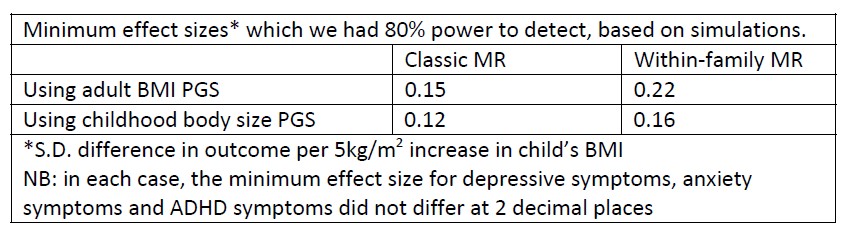
2) They used the correlation between PGS and BMI to support the assertion that the former is a strong instrument. Were the reported correlations calculated across all individuals? Since we know that stratification, assortative mating, and indirect effects can inflate these correlations, perhaps a more unbiased estimate would be the proportion of children's BMI variance explained by their PGS conditioned on the parents' PGS. This should also be the estimate used in power calculations.
The manuscript has been updated to quote Sanderson-Windmeijer conditional R2 values: the proportion of BMI variance explained by the BMI PGS for each member of a trio, conditional on the PGS of the other members of the trio, and all genetic covariates included in within-family models. Similarly, we now show Sanderson-Windmeijer conditional F-statistics for a model including the child, mother, and father’s BMI instrumented by the child, mother, and father’s PGS.
3) In testing the association of mothers' and fathers' BMI with children's symptoms, the authors used a multivariable linear regression conditioning on the child's own BMI. Was the other parent's BMI (either by itself or using the polygenic score) included as a covariate in the multivariable and MR models? This was not entirely clear from the text or from Fig. 2. I suspect that if there were assortative mating on BMI in the parent's generation, the effect of any one parent's BMI on the child's symptoms might be inflated unless the other parent's BMI was included as a covariate (assuming both mother's and father's BMI affect the child's symptoms).
Non-genetic models include both the mother and father’s phenotypic BMI as well as the child’s, allowing estimation of conditional effects of all three. This controls for assortative mating as noted by the reviewer. This was not previously clear - all relevant text and figure captions have been updated to clarify this.
4) They report no evidence of cross-trait assortative mating in the parents generation. The power to detect cross-trait assortative mating in the parents' generation using PGS would depend on the actual strength of assortative mating and the respective proportions of trait variance explained by PGS. Could the authors provide an estimate of the power for this test in their sample?
We have updated the discussion of assortative mating (in both the results and the discussion section) to note possible limitations of power and clarify that that this approach to examining assortment may not capture its full extent.
The relevant part of the results section now reads:
“In the parents’ generation, phenotypes were associated within parental pairs, consistent with assortative mating on these traits (Appendix 1 – Table 5). Adjusted for ancestry and other genetic covariates, maternal and paternal BMI were positively associated (beta: 0.23, 95%CI: 0.22,0.25, p<0.001), as were maternal and paternal depressive symptoms (beta: 0.18, 95%CI: 0.16,0.20, p<0.001), and maternal and paternal ADHD symptoms (beta: 0.11, 95%CI: 0.09,0.13, p<0.001). Consistent with cross-trait assortative mating, there was an association of mother’s BMI with father’s ADHD symptoms (beta: 0.03, 95%CI: 0.02,0.05, p<0.001) and mother’s ADHD symptoms with father’s depressive symptoms (beta: 0.05,95%CI: 0.05,0.06, p<0.001). Phenotypic associations can reflect the influence of one partner on another as well as selection into partnerships, but regression models of paternal polygenic scores on maternal polygenic scores also pointed to a degree of assortative mating. Adjusted for ancestry and genotyping covariates, there were small associations between parents’ BMI polygenic scores (beta: 0.01, 95%CI: 0.00,0.02, p=0.02 for the adult BMI PGS, and beta: 0.01, 95%CI: 0.00,0.02, p=0.008 for the childhood body size PGS), and of the mother’s childhood body size PGS with the father’s ADHD PGS (beta: 0.01, 95%CI: 0.00,0.02, p=0.03). We did not detect associations with pairs of other polygenic scores, which may be due to insufficient statistical power.”
And the relevant part of the discussion section now reads:
“We found some genomic evidence of assortative mating for BMI, and cross-trait assortative mating between BMI and ADHD, but not between other traits. However, associations between polygenic scores, which only capture some of the genetic variation associated with these phenotypes, may not capture the full extent of genetic assortment on these traits.”
5) Are the actual phenotypes (BMI, depression or ADHD) correlated between the parents? If so, would this not suffice as evidence of cross-trait assortative mating? It is known that the genetic correlation between parents as a result of assortative mating is a function of the correlation in their phenotypes and the heritabilities underlying the two traits (e.g., see Yengo and Visscher 2018). An alternative way to estimate the genetic correlation between parents without using PGS (which is noisy and therefore underpowered) would be to use the phenotypic correlation and heritability estimated using GREML or LDSC. Perhaps this is outside the scope of the paper but I would like to hear the author's thoughts on this.
Associations between maternal and paternal phenotypes are consistent with a degree of assortative mating (shown below). These results have added to Appendix 1 - Table 5, which also shows associations between maternal and paternal polygenic scores, and methods and results updated accordingly (see quoted text in response to the comment above). For comparability, both sets of results are based on regression models adjusting for the mother’s and father’s ancestry PCs and genotyping covariates. We agree that analysis of assortative mating using GREML or LDSC is out of scope for this paper. As noted above, we have updated the discussion to acknowledge the limitations of the approach taken:
‘We found some genomic evidence of assortative mating for BMI, and cross-trait assortative mating between BMI and ADHD, but not between other traits. However, associations between polygenic scores, which only capture some of the genetic variation associated with these phenotypes, may not capture the full extent of genetic assortment on these traits.’
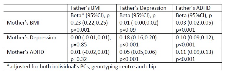
6) It would be helpful to include power calculations for the MR-Egger intercept estimates.
As with our response to the comments above, post-hoc power calculations are redundant, as all the information about the power of our analysis, including the MR-Egger is indicated by the standard errors and confidence intervals. MR-Egger is less precise than other estimators, as is made clear from the wide confidence intervals reported in the relevant tables (Appendix 1 - Tables 8 and 9). However, we have now updated the discussion to give more weight to this as a limitation. The discussion of pleiotropy in the final paragraph of the discussion now reads:
‘While robustness checks found little evidence of pleiotropy, these methods rely on assumptions. Moreover, MR-Egger is known to give imprecise estimates (Burgess and Thompson 2017), and confidence intervals from MR-Egger models were wide. Thus, pleiotropy cannot be ruled out.’
Similarly, we have updated the relevant line of the results section, which now reads:
‘MR-Egger models found little evidence of horizontal pleiotropy, although MR-Egger estimates were imprecise (Appendix 1 - Tables 8 and 9).’
7) Finally, what is the correlation between PGS and genetic PCs/geography in their sample? A correlation might provide evidence to support the point that classic MR effects are inflated due to stratification.
Figures presenting the association of the child’s BMI polygenic scores and their PCs have been added to the supplementary information as Appendix 1 - Figure 2 and Appendix 1 - Figure 3. Consistent with an influence of residual stratification, a regression of the child’s BMI polygenic scores against their ancestry PCs (adjusting for genotyping centre and chip) found that 7 of the 20 PCs were associated at p<0.05 with the adult BMI PGS, and 8 of 20 with the childhood body size PGS (under the null hypothesis, we would expect one association in each case). When parental polygenic scores were added to the models, these associations attenuated towards to null.
Author Response
Reviewer #1 (Public Review):
This manuscript seeks to identify the mechanism underlying priority effects in a plantmicrobe-pollinator model system and to explore its evolutionary and functional consequences. The manuscript first documents alternative community states in the wild: flowers tend to be strongly dominated by either bacteria or yeast but not both. Then lab experiments are used to show that bacteria lower the nectar pH, which inhibits yeast - thereby identifying a mechanism for the observed priority effect. The authors then perform an experimental evolution unfortunately experiment which shows that yeast can evolve tolerance to a lower pH. Finally, the authors show that low-pH nectar reduces pollinator consumption, suggesting a functional impact on the plant-pollinator system. Together, these multiple lines of evidence build a strong case that pH has far-reaching effects on the microbial community and beyond.
The paper is notable for the diverse approaches taken, including field observations, lab microbial competition and evolution experiments, genome resequencing of evolved strains, and field experiments with artificial flowers and nectar. This breadth can sometimes seem a bit overwhelming. The model system has been well developed by this group and is simple enough to dissect but also relevant and realistic. Whether the mechanism and interactions observed in this system can be extrapolated to other systems remains to be seen. The experimental design is generally sound. In terms of methods, the abundance of bacteria and yeast is measured using colony counts, and given that most microbes are uncultivable, it is important to show that these colony counts reflect true cell abundance in the nectar.
We have revised the text to address the relationship between cell counts and colony counts with nectar microbes. Specifically, we point out that our previous work (Peay et al. 2012) established a close correlation between CFUs and cell densities (r2 = 0.76) for six species of nectar yeasts isolated from D. aurantiacus nectar at Jasper Ridge, including M. reukaufii.
As for A. nectaris, we used a flow cytometric sorting technique to examine the relationship between cell density and CFU (figure supplement 1). This result should be viewed as preliminary given the low level of replication, but this relationship also appears to be linear, as shown below, indicating that colony counts likely reflect true cell abundance of this species in nectar.
It remains uncertain how closely CFU reflects total cell abundance of the entire bacterial and fungal community in nectar. However, a close association is possible and may be even likely given the data above, showing a close correlation between CFU and total cell count for several yeast species and A. nectaris, which are indicated by our data to be dominant species in nectar.
We have added the above points in the manuscript (lines 263-264, 938-932).
The genome resequencing to identify pH-driven mutations is, in my mind, the least connected and developed part of the manuscript, and could be removed to sharpen and shorten the manuscript.
We appreciate this perspective. However, given the disagreement between this perspective and reviewer 2’s, which asks for a more expanded section, we have decided to add a few additional lines (lines 628-637), briefly expanding on the genomic differences between strains evolved in bacteria-conditioned nectar and those evolved in low-pH nectar.
Overall, I think the authors achieve their aims of identifying a mechanism (pH) for the priority effect of early-colonizing bacteria on later-arriving yeast. The evolution and pollinator experiments show that pH has the potential for broader effects too. It is surprising that the authors do not discuss the inverse priority effect of early-arriving yeast on later-arriving bacteria, beyond a supplemental figure. Understandably this part of the story may warrant a separate manuscript.
We would like to point out that, in our original manuscript, we did discuss the inverse priority effects, referring to relevant findings that we previously reported (Tucker and Fukami 2014, Dhami et al. 2016 and 2018, Vannette and Fukami 2018). Specifically, we wrote that: “when yeast arrive first to nectar, they deplete nutrients such as amino acids and limit subsequent bacterial growth, thereby avoiding pH-driven suppression that would happen if bacteria were initially more abundant (Tucker and Fukami 2014; Vannette and Fukami 2018)” (lines 385-388). However, we now realize that this brief mention of the inverse priority effects was not sufficiently linked to our motivation for focusing mainly on the priority effects of bacteria on yeast in the present paper. Accordingly, we added the following sentences: “Since our previous papers sought to elucidate priority effects of early-arriving yeast, here we focus primarily on the other side of the priority effects, where initial dominance of bacteria inhibits yeast growth.” (lines 398-401).
I anticipate this paper will have a significant impact because it is a nice model for how one might identify and validate a mechanism for community-level interactions. I suspect it will be cited as a rare example of the mechanistic basis of priority effects, even across many systems (not just pollinator-microbe systems). It illustrates nicely a more general ecological phenomenon and is presented in a way that is accessible to a broader audience.
Thank you for this positive assessment.
Reviewer #2 (Public Review):
The manuscript "pH as an eco-evolutionary driver of priority effects" by Chappell et al illustrates how a single driver-microbial-induced pH change can affect multiple levels of species interactions including microbial community structure, microbial evolutionary change, and hummingbird nectar consumption (potentially influencing both microbial dispersal and plant reproduction). It is an elegant study with different interacting parts: from laboratory to field experiments addressing mechanism, condition, evolution, and functional consequences. It will likely be of interest to a wide audience and has implications for microbial, plant, and animal ecology and evolution.
This is a well-written manuscript, with generally clear and informative figures. It represents a large body and variety of work that is novel and relevant (all major strengths).
We appreciate this positive assessment.
Overall, the authors' claims and conclusions are justified by the data. There are a few things that could be addressed in more detail in the manuscript. The most important weakness in terms of lack of information/discussion is that it looks like there are just as many or more genomic differences between the bacterial-conditioned evolved strains and the low-pH evolved strains than there are between these and the normal nectar media evolved strains. I don't think this negates the main conclusion that pH is the primary driver of priority effects in this system, but it does open the question of what you are missing when you focus only on pH. I would like to see a discussion of the differences between bacteria-conditioned vs. low-pH evolved strains.
We agree with the reviewer and have included an expanded discussion in the revised manuscript [lines 628-637]. Specifically, to show overall genomic variation between treatments, we calculated genome-wide Fst comparing the various nectar conditions. We found that Fst was 0.0013, 0.0014, and 0.0015 for the low-pH vs. normal, low pH vs. bacteria-conditioned, and bacteria-conditioned vs. normal comparisons, respectively. The similarity between all treatments suggests that the differences between bacteria-conditioned and low pH are comparable to each treatment compared to normal. This result highlights that, although our phenotypic data suggest alterations to pH as the most important factor for this priority effect, it still may be one of many affecting the coevolutionary dynamics of wild yeast in the microbial communities they are part of. In the full community context in which these microbes grow in the field, multi-species interactions, environmental microclimates, etc. likely also play a role in rapid adaptation of these microbes which was not investigated in the current study.
Based on this overall picture, we have included additional discussion focusing on the effect of pH on evolution of stronger resistance to priority effects. We compared genomic differences between bacteria-conditioned and low-pH evolved strains, drawing the reader’s attention to specific differences in source data 14-15. Loci that varied between the low pH and bacteria-conditioned treatments occurred in genes associated with protein folding, amino acid biosynthesis, and metabolism.
Reviewer #3 (Public Review):
This work seeks to identify a common factor governing priority effects, including mechanism, condition, evolution, and functional consequences. It is suggested that environmental pH is the main factor that explains various aspects of priority effects across levels of biological organization. Building upon this well-studied nectar microbiome system, it is suggested that pH-mediated priority effects give rise to bacterial and yeast dominance as alternative community states. Furthermore, pH determines both the strengths and limits of priority effects through rapid evolution, with functional consequences for the host plant's reproduction. These data contribute to ongoing discussions of deterministic and stochastic drivers of community assembly processes.
Strengths:
Provides multiple lines of field and laboratory evidence to show that pH is the main factor shaping priority effects in the nectar microbiome. Field surveys characterize the distribution of microbial communities with flowers frequently dominated by either bacteria or yeast, suggesting that inhibitory priority effects explain these patterns. Microcosm experiments showed that A. nectaris (bacteria) showed negative inhibitory priority effects against M. reukaffi (yeast). Furthermore, high densities of bacteria were correlated with lower pH potentially due to bacteria-induced reduction in nectar pH. Experimental evolution showed that yeast evolved in low-pH and bacteria-conditioned treatments were less affected by priority effects as compared to ancestral yeast populations. This potentially explains the variation of bacteria-dominated flowers observed in the field, as yeast rapidly evolves resistance to bacterial priority effects. Genome sequencing further reveals that phenotypic changes in low-pH and bacteriaconditioned nectar treatments corresponded to genomic variation. Lastly, a field experiment showed that low nectar pH reduced flower visitation by hummingbirds. pH not only affected microbial priority effects but also has functional consequences for host plants.
We appreciate this positive assessment.
Weaknesses:
The conclusions of this paper are generally well-supported by the data, but some aspects of the experiments and analysis need to be clarified and expanded.
The authors imply that in their field surveys flowers were frequently dominated by bacteria or yeast, but rarely together. The authors argue that the distributional patterns of bacteria and yeast are therefore indicative of alternative states. In each of the 12 sites, 96 flowers were sampled for nectar microbes. However, it's unclear to what degree the spatial proximity of flowers within each of the sampled sites biased the observed distribution patterns. Furthermore, seasonal patterns may also influence microbial distribution patterns, especially in the case of co-dominated flowers. Temperature and moisture might influence the dominance patterns of bacteria and yeast.
We agree that these factors could potentially explain the presented results. Accordingly, we conducted spatial and seasonal analyses of the data, which we detail below and include in two new paragraphs in the manuscript [lines 290-309].
First, to determine whether spatial proximity influenced yeast and bacterial CFUs, we regressed the geographic distance between all possible pairs of plants to the difference in bacterial or fungal abundance between the paired plants. If plant location affected microbial abundance, one should see a positive relationship between distance and the difference in microbial abundance between a given pair of plants: a pair of plants that were more distantly located from each other should be, on average, more different in microbial abundance. Contrary to this expectation, we found no significant relationship between distance and the difference in bacterial colonization (A, p=0.07, R2=0.0003) and a small negative association between distance and the difference in fungal colonization (B, p<0.05, R2=0.004). Thus, there was no obvious overall spatial pattern in whether flowers were dominated by yeast or bacteria.
Next, to determine whether climatic factors or seasonality affected the colonization of bacteria and yeast per plant, we used a linear mixed model predicting the average bacteria and yeast density per plant from average annual temperature, temperature seasonality, and annual precipitation at each site, the date the site was sampled, and the site location and plant as nested random effects. We found that none of these variables were significantly associated with the density of bacteria and yeast in each plant.
To look at seasonality, we also re-ordered Fig 2C, which shows the abundance of bacteria- and yeast-dominated flowers at each site, so that the sites are now listed in order of sampling dates. In this re-ordered figure, there is no obvious trend in the number of flowers dominated by yeast throughout the period sampled (6.23 to 7/9), giving additional indication that seasonality was unlikely to affect the results.
Additionally, sampling date does not seem to strongly predict bacterial or fungal density within each flower when plotted.
These additional analyses, now included (figure supplements 2-4) and described (lines 290-309) in the manuscript, indicate that the observed microbial distribution patterns are unlikely to have been strongly influenced by spatial proximity, temperature, moisture, or seasonality, reinforcing the possibility that the distribution patterns instead indicate bacterial and yeast dominance as alternative stable states.
The authors exposed yeast to nectar treatments varying in pH levels. Using experimental evolution approaches, the authors determined that yeast grown in low pH nectar treatments were more resistant to priority effects by bacteria. The metric used to determine the bacteria's priority effect strength on yeast does not seem to take into account factors that limit growth, such as the environmental carrying capacity. In addition, yeast evolves in normal (pH =6) and low pH (3) nectar treatments, but it's unclear how resistance differs across a range of pH levels (ranging from low to high pH) and affects the cost of yeast resistance to bacteria priority effects. The cost of resistance may influence yeast life-history traits.
The strength of bacterial priority effects on yeast was calculated using the metric we previously published in Vannette and Fukami (2014): PE = log(BY/(-Y)) - log(YB/(Y-)), where BY and YB represent the final yeast density when early arrival (day 0 of the experiment) was by bacteria or yeast, followed by late arrival by yeast or bacteria (day 2), respectively, and -Y and Y- represent the final density of yeast in monoculture when they were introduced late or early, respectively. This metric does not incorporate carrying capacity. However, it does compare how each microbial species grows alone, relative to growth before or after a competitor. In this way, our metric compares environmental differences between treatments while also taking into account growth differences between strains.
Here we also present additional growth data to address the reviewer’s point about carrying capacity. Our experiments that compared ancestral and evolved yeast were conducted over the course of two days of growth. In preliminary monoculture growth experiments of each evolved strain, we found that yeast populations did reach carrying capacity over the course of the two-day experiment and population size declined or stayed constant after three and four days of growth.
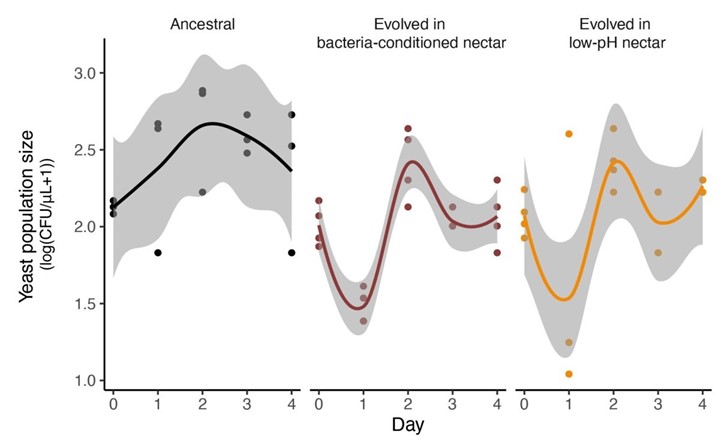
However, we found no significant difference in monoculture growth between the ancestral stains and any of the evolved strains, as shown in Figure supplement 12B. This lack of significant difference in monoculture suggests that differences in intrinsic growth rate do not fully explain the priority effects results we present. Instead, differences in growth were specific to yeast’s response to early arrival by bacteria.
We also appreciate the reviewer’s comment about how yeast evolves resistance across a range of pH levels, as well as the effect of pH on yeast life-history traits. In fact, reviewer #2 pointed out an interesting trade-off in life history traits between growth and resistance to priority effects that we now include in the discussion (lines 535-551) as well as a figure in the manuscript (Figure 8).
Author Response
Reviewer #2 (Public Review):
Schrecker, Castaneda and colleagues present cryo-EM structures of RFC-PCNA bound to 3'ss/dsDNA junction or nicked DNA stabilized by slowly hydrolyzable ATP analogue, ATPyS. They discover that PCNA can adopt an open form that is planar, different from previous models for the loading a sliding clamp. The authors also report a structure with closed PCNA, supporting the notion that closure of the sliding clamp does not require ATP hydrolysis. The structures explain how DNA can be threaded laterally through a gap in the PCNA trimer, as this process is supported by partial melting of the DNA prior to insertion. The authors also visualise and assign a function to the N-terminal domain in the Rfc1 subunit of the clamp loader, which they find modulates PCNA loading at the replication forks, in turn required for processive synthesis and ligation of Okazaki fragments.
This work is extremely well done, with several structures with resolutions better than 3Å, which a significant achievement given the dynamic nature of the PCNA ring loading process. To investigate the role of the N-terminal domain of Rfc1 in PCNA loading, the authors use in vitro reconstitution of the entire DNA replication reaction, which is a powerful method to identify specific defects in Okazaki fragment synthesis and ligation.
Important issues
- Figure 3B,D,F. I would find them much more informative if the authors showed the overlay between atomic model and cryo-EM density in the main figure. If the figure becomes too busy, the authors could decide to just add additional panels with the overlay as well as the atomic models alone. I do not think that showing segmented density for the DNA alone, as done is Figure 6C is sufficient. Also including the density for e.g. residues Trp638 and Phe582 seems important.
We thank the reviewer for the suggestion. However, we have been unable to establish a way to show the density for both the protein and DNA in a meaningful manner due to the large number of atoms in the fields of view. For an example, please see Figure 1, which corresponds to Figure 3H. To aid the reader, we have revised several of the Figures and Figure Supplements to include density for the DNA.
Consistent with our structures, recent work from the Kelch group has identified Trp638 and Phe582 as facilitating DNA base flipping (Gaubitz et al., 2022a). Despite the role in base flipping, no growth defects were observed in cells in which either of these residues were mutated and thus their functional role and the role of DNA base-flipping remains unclear.
- Cryo-EM samples preparation included substoichiometric RPA, which has been shown to promote DNA loading of PCNA by RFC. Would the authors expect a subset of PCNA-RFC-DNA particles to contain RPA as well? The glycerol gradient gel indicates that, at least in fraction 5, a complex might exist. If the authors think that the particles analyzed cannot contain RPA, it would be useful to mention this.
We have no evidence to suggest that RPA cannot be present in the imaged particles. We have revised the text (lines 150 - 152) clarify that while RPA was present in the sample, we did not observe any density that could not be assigned to either DNA, RFC or PCNA. We therefore suggest that RPA does not interact with the complex in a stable manner.
- Published kinetic data indicate that ATP hydrolysis occurs before clamp closure. To incorporate this notion in their model, the authors suggest that ATP hydrolysis might promote PCNA closure by disrupting the planar RFC:PCNA interaction surface and hence the dynamic interaction of PCNA with Rfc2 and -5 in the open state. In addition, ATP hydrolysis promotes RFC disengagement from PCNA-DNA by reverting from a planar to an out-of-plane state. This model appears reasonable and nicely combines published data with the new findings reported by the authors. However, the model is oversimplified in Figure 6, where the only depicted effect of ATP hydrolysis is RFC release. Perhaps the authors could use the figure caption to acknowledge that ATP hydrolysis likely still has a role in facilitating PCNA closure.
We have revised Figure 6 to show that DNA hydrolysis may occur either before or after ring closure.
- Can the authors explain what steps should be taken to describe PCNA loading by RFC in conditions where ATP hydrolysis is permitted? How would such experiments further inform the molecular mechanism for the loading of the PCNA clamp?
As highlighted in point 3 above and by the other reviewers, ATP and ATPgS may alter the behavior and energetic landscape of RFC. In our studies, ATPgS was added trap the complex in a pre-hydrolysis state in which all components are assembled. We have added a section to the discussion noting the potential differences and highlighting the need for future studies to better elucidate the role of nucleotide hydrolysis. To achieve a hydrolysis competent complex, one could apply time-resolved cryo-EM approaches where the complex is formed on the grids and quickly vitrified. Such an approach, particularly if coupled with stopped-flow kinetic analyses, may provide additional insights in the kinetics of loading of PCNA onto DNA by RFC.
Author Response
The following is the authors’ response to the original reviews.
Reviewer #1 (Recommendations For The Authors):
The brain-machine interface used in this study differs from typical BMIs in that it's not intended to give subjects voluntary control over their environment. However, it is possible that rats may become aware of their ability to manipulate trial start times using their neural activity. Is there any evidence that the time required to initiate trials on high-coherence or low-coherence trials decreases with experience?
This is a great question. First, we designed the experiment to avoid this possibility. Rats were experienced on the sequence of the automatic maze both pre and post implantation (totaling to weeks of pre-training and habituation). As such, the majority of the trials ever experienced by the rat were not controlled by their neural activity. During BMI experimentation, only 10% of trials were triggered during high coherence states and 10% for low coherence states, leaving ~80% of trials not controlled by their neural activity. We also implemented a pseudo-randomized trial sequence. When considered together, we specifically designed this experiment to avoid the possibility that rats would actively use their neural activity to control the maze.
Second, we had a similar question when collecting data for this manuscript and so we conducted a pilot experiment. We took 3 rats from experiment #1 (after its completion) and we required them to perform “forced-runs” over the course of 3-4 days, a task where rats navigate to a reward zone and are rewarded with a chocolate pellet. The trajectory on “forced-runs” is predetermined and rats were always rewarded for navigating along the predetermined route. Every trial was initiated by strong mPFC-hippocampal theta coherence. We were curious as to whether time-to-trial-onset would decrease if we repeatedly paired trial onset to strong mPFC-hippocampal theta coherence. 1 out of 3 rats (rat 21-35) showed a significant correlation between time-to-trial onset and trial number, indicating that our threshold for strong mPFC-hippocampal theta coherence was being met more quickly with experience (Figure R1A). When looking over sessions and rats, there was considerable variability in the magnitude of this correlation and sometimes even the direction (Figure R1B). As such, the degree to which rat 21-35 was aware of controlling the environment by reaching strong mPFC-hippocampal theta coherence is unclear, but this question requires future experimentation.
Author response image 1.
Strong mPFC-hippocampal theta coherence was used to control trial onset for the entirety of forced-navigation sessions. Time-to-trial onset is a measurement of how long it took for strong coherence to be met. A) Time-to-trial onset was averaged across sessions for each rat, then plotted as a function of trial number (within-session experience on the forced-runs task). Rat 21-35 showed a significant negative correlation between time-to-trial onset and trial number, indicating that time-to-coherence reduced with experience. The rest of the rats did not display this effect. B) Correlation between trial-onset and trial number (y-axis; see A) across sessions (x-axis). A majority of sessions showed a negative correlation between time-to-trial onset and trial number, like what was seen in (A), but the magnitude and sometimes direction of this effect varied considerably even within an animal.
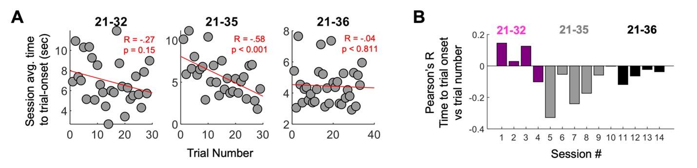
Is there any evidence that rats display better performance on trials with random delays in which HPC-PFC coherence was naturally elevated?
This question is now addressed in Extended Figure 5 and discussed in the section titled “strong prefrontal-hippocampal theta coherence leads to correct choices on a spatial working memory task”.
The introduction frames this study as a test of the "communication through coherence" hypothesis. In its strongest form, this hypothesis states that oscillatory synchronization is a pre-requisite for inter-areal communication, i.e. if two areas are not synchronized, they cannot transfer information. Recent experimental evidence shows this relationship is more likely inverted-coherence is a consequence of inter-areal interactions, rather than a cause. See Schneider et al. (DOI: 10.1016/j.neuron.2021.09.037) and Vinck et al. (10.1016/j.neuron.2023.03.015) for a more in-depth explanation of this distinction. The authors should expand their treatment of this hypothesis in light of these findings.
Our introduction and discussions have sections dedicated to these studies now.
Figure 6 - It would be much more intuitive to use the labels "Rat 1", "Rat 2", and "Rat 3"; the "21-4X" identifiers are confusing.
This was corrected in the paper.
Figure 6C - The sub-plots within this figure are rather small and difficult to interpret. The figure would be easier to parse if the data were presented as a heatmap of the ratio of theta power during blue vs. red stim, with each pixel corresponding to one channel.
This suggestion was implemented in the paper. See Fig 6C. Extended Fig. 8 now shows the power spectra as a function of recording shank and channel.
Ext. Figure 2B - What happens during an acquisition failure? Instead of "Amount of LFP data," consider using "Buffer size".
Corrected.
Ext. Figure 2D-E - Instead of "Amount of data," consider using "Window size"
Referred to as buffer size.
Ext. Figure 2E - y-axis should extend down to 4 Hz. Are all of the last four values exactly at 8 Hz?
Yes. Values plateau at 8Hz. These data represent an average over ~50 samples.
Ext. Figure 2F - consider moving this before D/E, since those panels are summaries of panel F
Corrected.
Ext. Figure 4A - ANOVA tells you that accuracy is impacted by delay duration, but not what that impact is. A post-hoc test is required to show that long delays lead to lower accuracy than short ones. Alternatively, one could compute the correlation between delay duration and proportion correctly for each mouse, and look for significant negative values.
We included supplemental analyses in Extended Fig. 4
Reviewer #2 (Recommendations For The Authors):
The authors should replace terms that suggest a causal relationship between PFC-HPC synchrony and behavior, such as 'leads to', 'biases', and 'enhances' with more neutral terms.
Causal implications were toned down and wherever “leads” or “led” remains, we specifically mean in the context of coherence being detected prior to a choice being made.
The rationale for the analysis described in the paragraph starting on line 324, and how it fits with the preceding results, was not clear to me. The authors also write at the start of this paragraph "Given that mPFC-hippocampal theta coherence fluctuated in a periodical manner (Extended Fig. 5B)", but this figure only shows example data from 2 trials.
The reviewer is correct. While we point towards 3 examples in the manuscript now, we focused this section on the autocorrelation analysis, which did not support our observation as we noticed a rather linear decay in correlation over time. As such, the periodicity observed was almost certainly a consequence of overlapping data in the epochs used to calculate coherence rather than intrinsic periodicity.
Shortly after the start of the results section (line 112), the authors go into a very detailed description of how they validated their BMI without first describing what the BMI actually does. This made this and the subsequent paragraphs difficult to follow. I suggest the authors start with a general description of the BMI (and the general experiment) before going into the details.
Corrected. See first paragraph of “Development of a closed-loop…”.
In Figure 2C, as expected, around the onset of 'high' coherence trials, there is an increase in theta coherence but this appears to be very transient. However, it is unclear what the heatmap represents: is it a single trial, single session, an average across animals, or something else? In Figure 3F, however, the increase appears to be much more sustained.
The sample size was rats for every panel in this figure. This was clarified at the end of Fig. 3.
In Figure 2D, it was not clear to me what units of measurement are used when the averages and error bars are calculated. What is the 'n' here? Animals or sessions? This should be made clear in this figure as well as in other figures.
The sample size is rats. This is now clarified at the end of Fig 2.
Describing the study of Jones and Wilson (2005), the authors write: "While foundational, this study treated the dependent variable (choice accuracy) as independent to test the effect of choice outcome on task performance." (line 83) It was not clear to me what is meant by "dependent" and "independent" here. Explaining this more clearly might clarify how the authors' study goes beyond this and other previous studies.
The reviewer is correct. A discussion on independent/dependent variables in the context of rationale for our experiment was removed.
Reviewer #3 (Recommendations For The Authors):
As explained in the public review, my comments mainly concern the interpretation of the experimental paradigm and its link with previous findings. I think modifying these in order to target the specific advance allowed by the paradigm would really improve the match between the experimental and analytical data that is very solid and the author's conclusions.
Concerning the paradigm, I recommend that the authors focus more on their novel ability to clearly dissociate the functional role of theta coherence prior to the choice as opposed to induced by the choice. Currently, they explain by contrasting previous studies based on dependent variables whereas their approach uses an independent variable. I was a bit confused by this, particularly because the task variable is not really independent given that it's based on a brain-driven loop. Since theta coherence remains correlated with many other neurophysiological variables, the results cannot go beyond showing that leading up to the decision it correlates with good choice accuracy, without providing evidence that it is theta coherence itself that enhances this accuracy as they suggest in lines 93-94.
The reviewer is correct. A discussion on independent/dependent variables in the context of rationale for our experiment was removed.
Regarding previous results with muscimol inactivation, I recommend that the authors expand their discussion on this point. I think that their correlative data is not sufficient to conclude as they do that despite "these structures being deemed unnecessary" (based on causal muscimol experiments), they "can still contribute rather significantly" since their findings do not show a contribution, merely a correlation. This extra discussion could include possible explanations of the apparent, and thought-provoking discrepancies that they uncover such as: theta coherence may be a correlate of good accuracy without an underlying causal relation, theta coherence may always correlate with good accuracy but only be causally important in some tasks related to spatial working memory or, since muscimol experiments leave the brain time to adapt to the inactivation, redundancy between brain areas may mask their implication in the physiological context in certain tasks (see Goshen et al 2011).
The second paragraph of the discussion is now dedicated to this.
Possible further analysis :
- In Extended 4A the authors show that performance drops with delay duration. It would be very interesting to see this graph with the high coherence / low coherence / yoked trials to see if the theta coherence is most important for longer trials for example.
This is a great suggestion. Due to 10% of trials being triggered by high coherence states, our sample size precludes a robust analysis as suggested. Given that we found an enhancement effect on a task with minimal spatial working memory requirements (Fig. 4), it seems that coherence may be a general benefit or consequence of choice processes. Nonetheless, this remains an important question to address in a future study.
- Figure 6: The authors explain in the text that although the effect of stimulation of VMT is variable, overall VMT activation increased PFC-HPC coherence. I think in the figure the results are only shown for one rat and session per panel. It would be interesting to add a figure including their whole data set to show the overall effect as well as the variability.
The reviewer is correct and this comment promoted significant addition of detail to the manuscript. We have added an extended figure (Ext. Fig. 9) showing our VMT stimulation recording sessions. We originally did not include these because we were performing a parameter search to understanding if VMT stimulation could increase mPFC-hippocampal theta coherence. The results section was expanded accordingly.
Changes to writing / figures :
- The paper by Eliav et al, 2018 is cited to illustrate the universality of coupling between hippocampal rhythms and spikes whereas the main finding of this paper is that spikes lock to non-rhythmic LFP in the bat hippocampus. It seems inappropriate to cite this paper in the sentence on line 65.
We agree with the reviewer and this citation was removed.
- Line 180 when explaining the protocol, it would help comprehension if the authors clearly stated that "trial initiation" means opening the door to allow the rat to make its choice. I was initially unfamiliar with the paradigm and didn't figure this out immediately.
We added a description to the second paragraph of our first results section.
- Lines 324 and following: the analysis shows that there is a slow decay over around 2s of the theta coherence but not that it is periodical (as in regularly occurring in time), this would require the auto-correlation to show another bump at the timescale corresponding to the period of the signal. I recommend the authors use a different terminology.
This comment is now addressed above in our response to Reviewer #2.
- Lines 344: I am not sure why the stable theta coherence levels during the fixed delay phase show that the link with task performance is "through mechanisms specific to choice". Could the authors elaborate on this?
We elaborated on this point further at the end of “Trials initiated by strong prefrontal-hippocampal theta coherence are characterized by prominent prefrontal theta rhythms and heightened pre-choice prefrontal-hippocampal synchrony”
- Line 85: "independent to test the effect of choice outcome on task performance." I think there is a typo here and "choice outcome" should be "theta coherence".
The sentence was removed in the updated draft.
Author Response
Reviewer 1
Employing in vitro and Drosophila model, the authors interrogate which domain of Hsp27 binds to which region on Tau, and how these interactions facilitate the proteinaceous aggregation. They utilized various biochemical, biophysical, cellular, and genetic tools to dissect the association, and identified the structural basis for the specific recognition of Hsp27 to pathogenic p-Tau. Conceivably, Hsp27 may play some role in preventing Tau abnormal aggregation and p-Tau pathology in AD. Overall, the data support the main claim, especially, the biophysical data are very impressive. Nevertheless, the manuscript could be strengthened by complementary cellular or biochemical methods for validation. For example, the authors can use a stably transfected Tau cell line to interrogate Hsp27's role in its cellular aggregation or proteinaceous inclusions by immunoblotting. Immunofluorescent and immunohistochemical staining and IB with different antibodies may be conducted to validate the observations.
REPLY: We sincerely thank the reviewer for the positive assessment of our work, and for providing very insightful suggestions. We appreciate the reviewer for considering our biophysical data to be impressive. We totally agree with the reviewer that the work could be strengthened by complementary cellular methods for validation. In our work, we used the Drosophila tauopathy model, where expression of human TauR406W in the Drosophila nervous system leads to age-dependent neurodegeneration recapitulating some of the salient features of tauopathy in FTDP-171,2, to interrogate the role of Hsp27 in aggregation and proteinaceous inclusions of pTau.
In our Drosophila Tau model study, three different antibodies including a total Tau antibody 5A63, a pTauSer262 specific antibody4, and a hyper-phosphorylated Tau antibody AT8 that recognizes hyper-phosphorylation of Tau at Ser202 and Thr205 sites5 were used in western blot analysis to explore the role of Hsp27. As shown in Figure R1-1A and 1B, overexpression of Hsp27 significantly reduced the level of both pTauSer262 and hyper-phosphorylated Tau at both 2 and 10 days after eclosion (DAE). In addition, we further examined the morphology of the fly brain as well as the accumulation of hyper-phosphorylated Tau by immunofluorescence staining. Consistent with previous findings, brains with neuronal expression of TauR406W exhibited an accumulation of filamentous pTau and a reduction of brain neuropil size indicative of neurodegeneration (Figure R11C-F). Importantly, overexpression of Hsp27 restored the size of brain neuropil and suppressed the accumulation of filamentous pTau (Figure R1-1C-F), suggesting that Hsp27 protects against mutant TauR406W - induced neurodegeneration. Taken together, our Drosophila results show that Hsp27 protects against synaptic dysfunction in a Drosophila tauopathy model by reducing pTau aggregation, which well supports our biophysical data.

Figure R1-1 Hsp27 reduces pTau level and protects against pTau-induced synaptopathy in Drosophila. (This figure represents Fig. 2A-F in the revised manuscript) (A) Brain lysates of 2 and 10 days after eclosion (DAE) wild-type (WT) flies (lanes 1 and 6), flies expressing human Tau with GFP (lanes 4 and 9), or human Tau with Hsp27 (lanes 5 and 10) in the nervous system were probed with antibodies for disease-associated phospho-tau epitopes S262, Ser202/Thr205 (AT8), and total Tau (5A6). Actin was probed as a loading control. Brain lysates of flies carrying only UAS elements were loaded for control (lanes 2, 3, 7, and 8). (B) Quantification of protein fold changes in (A). The levels of Tau species were normalized to actin. Fold changes were normalized to the Tau+GFP group at 2 DAE. n = 3. (C) Brains of WT flies or flies expressing Tau+GFP or Tau+Hsp27 in the nervous system at 2 DAE were probed for AT8 (heatmap) and Hsp27 (green), and stained with DAPI (blue). Scale bar, 30 μm. (D-F) Quantification of the Hsp27 intensity (D, data normalized to WT), brain optic lobe size (E), and AT8 intensity (F, data normalized to the Tau+GFP group). n = 4.
Reviewer 2
Abnormal accumulation and aggregation of amyloid-β protein are one of the main pathological hallmarks of Alzheimer's disease. It is well known that molecular chaperones play central roles in regulating tau function and amyloid assembly in disease. In this manuscript, Zhang, Zhu, Lu, Liu, et al., have investigated that Hsp27, a member of the small heat shock protein, specifically binds to phosphorylated Tau, which prevents pTau fibrillation in vitro and in a Drosophila tauopathy model. Using NMR spectroscopy and cross-linking mass spectrometry, the authors found that the N-terminal domain of Hsp27 directly binds to phosphorylation sites of pTau. Overall, the study is important and provides the demonstration of interactions between Hsp27 and pTau.
REPLY: We sincerely thank the reviewer for the positive remarks of this work, and appreciate that the reviewer summarizes the major conclusions of our manuscript, and evaluates our work is important in the area of fundamental biology of the interaction between chaperones and clients, and its implications in AD pathology.
Author Response
Reviewer #2 (Public Review):
Activation of TEAD-dependent transcription by YAP/TAZ has been implicated in the development and progression of a significant number of malignancies. For example, loss of function mutations in NF2 or LATS1/2 (known upstream regulators that promote YAP phosphorylation and its retention and degradation in the cytoplasm) promote YAP nuclear entry and association with TEAD to drive oncogenic gene transcription and occurs in >70% of mesothelioma patients. High levels of nuclear YAP have also been reported for a number of other cancer cell types. As such, the YAP-TEAD complex represents a promising target for drug discovery and therapeutic intervention. Based on the recently reported essential functional role for TEAD palmitoylation at a conserved cysteine site, several groups have successfully targeted this site using both reversible binding non-covalent TEAD inhibitors (i.e., flufenamic acid (FA), MGH-CP1, compound 2 and VT101~107), as well as covalent TEAD inhibitors (i.e., TED-347, DC-TEADin02, and K-975), which have been demonstrated to inhibit YAP-TEAD function and display antitumor activity in cells and in vivo.
Here, Fan et al. disclose the development of covalent TEAD inhibitors and report on the therapeutic potential of this class of agents in the treatment of TEAD-YAP-driven cancers (e.g., malignant pleural mesothelioma (MPM)). Optimized derivatives of a previously reported flufenamic acid-based acrylamide electrophilic warhead-containing TEAD inhibitor (MYF-01-37, Kurppa et al. 2020 Cancer Cell), which display improved biochemical- and cell-based potency or mouse pharmacokinetic profiles (MYF-03-69 and MYP-03-176) are described and characterized.
Strengths:
All of the authors' claims and conclusions are very well supported and justified by the data that is provided. Clear improvements in biochemical- and cell-based potencies have been made within the compound series. Cell-based selective activities in the HIPPO pathway defective versus normal/control cell types are established. Transcriptional effects and the regulation of BMF proapoptotic mRNA levels are characterized. A 1.68 A X-Ray co-crystal structure of MYF-03-69 covalently bound to TEAD1 via Cys359 is provided. In vivo efficacy in a relevant xenograft is demonstrated, using a 30 mg/kg, BID PO dose.
We thank the reviewer for appreciating and highlighting the strengths of our study.
Weaknesses:
Beyond the impact on BMF gene regulation, new biological insights reported here for this compound series are moderate. Progress and differentiation with respect to activity and/or ADME PK profiles relative to the very closely related and previously described (Keneda et al. 2020 Am J Cancer Res 10:4399. PMID 33415007) acrylamide-based covalent TEAD inhibitor K-975 (identical 11 nM cell-based potencies when compared head-to-head and identical reported in vivo efficacy doses of 30 mg/kg) is not entirely clear. Demonstration of on-target in vivo activity is lacking (e.g., impact on BMF gene expression at the evaluated exposure levels).
We thank the reviewer’s question. We have compared mouse liver microsome stability and hepatocyte stability of K-975 and MYF-03-176 and found that K-975 is metabolically less stable.
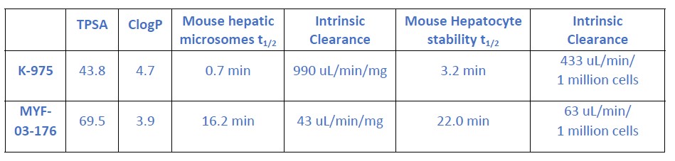
Consistently, when NCI-H226 cells derived xenograft mice were dosed with 30 mg/kg K-975 twice daily, the tumors kept growing and reach more than 1.5-fold volume on 14th day. While with the same dosage, MYF-03-176 showed a significant tumor regression. K-975 did not reach such efficacy even with 100 or 300 mg/kg twice daily, either in NCI-H226 or MSTO-211H CDX mouse model according to the paper (Keneda et al. 2020 Am J Cancer Res 10:4399).
To demonstrate the on-target in vivo activity, we tested expression of the TEAD downstream genes and BMF in tumor sample after 3-day BID treatment (PD study) and we observed reduction of CTGF, CYR61, ANKRD1 and an increase of BMF, which indicates an on-target activity in vivo.
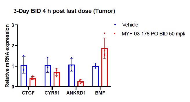
Author Response
Reviewer #2 (Public Review):
This paper by Angueyra, et al., adds to the field’s current understanding of photoreceptor specification and factors regulating opsin expression in vertebrates. Current models of specification of vertebrate photoreceptors are largely based on studies of mammals. However, a great number of animals including teleosts express a wider array of photoreceptor subtypes. Zebrafish for example have 4 distinct cone subtypes and rods. The approach is sound and the data are quite convincing. The only minor weaknesses are that the statistical analyses need to be revisited and the discussion should be a bit more focused.
To identify differentially expressed transcription factors, the authors performed bulk RNA-seq of pooled, hand-sorted photoreceptors. The selection criterion was tightly controlled to limit unhealthy cells and cellular debris from other photoreceptors subtypes. The pooling of cells provided a considerable depth of sequencing, orders of magnitude better than scSeq. The authors identified known transcription factors and several that appear to be novel or their role has not been determined. The data are made available on the PIs website as is a program to access and compare the gene expression data.
The authors then used CRISPR/Cas9 gene targeting of two known and several novel factors identified in their analysis for effects on cell fate decisions and opsin expression. Phenotyping performed on the injected larvae is possible, and the target genes were applied and sequenced to demonstrate the efficiency of the gene targeting. Targeting of 2 genes with know functions in photoreceptor specification in zebrafish, Tbx2b and Foxq2 resulted in the anticipated changes in cell fate, albeit, the strength of the alterations in cell fate in the F0 larvae appears to be less than the published phenotypes for the inherited alleles. Interestingly, the authors also identified the expression of an RH2 opsin in the SWS2 another cone type. The changes are subtle but important.
The authors then targeted tbx2a, the function of which was not known. The result is quite interesting as it matches the increase of rods and decrease of UV cones observed in tbx2b mutants. However, the injected animals also showed RH2 opsin expression but are now in the LWS cone subtype. These data suggest that Tbx2 transcription factors repress misexpression of opsins in the wrong cell type.
The authors also show that targeting additional differentially expressed factors does not affect photoreceptor fate or survival in the time frame investigated. These are important data to present. For these or any of the other targeted genes above, did the authors test for changes in photoreceptor number or survival?
We have attempted to address this point, but the answer is not clear cut. We used activated caspase-3 inmmunolabeling as a marker of apoptosis (Lusk and Kwan 2022). At 5 dpf, the age we chose to make quantifications, we don’t see an increase in activated caspase-3 positive cells when we compare control and tbx2a F0 mutants (Reviewer Figure 1A-B). Labeled cells are very rare and located near the ciliary marginal zone irrespective of genotype. This suggests that there is no detectable active death at this late stage of development in tbx2 F0 mutants. Earlier in development, at 3 dpf, when photoreceptor subtypes first appear, there is also a normal wave of apoptosis in the retina (Blume et al. 2020; Biehlmaier, Neuhauss, and Kohler 2001), resulting in many cells positive for activated caspase-3; our preliminary quantifications don’t show a marked increase in the number of labeled cells in tbx2a F0 mutants, but we consider that it’s likely that subtle effects might be obscured by the physiological wave of apoptosis (Reviewer Figure 1C-D).
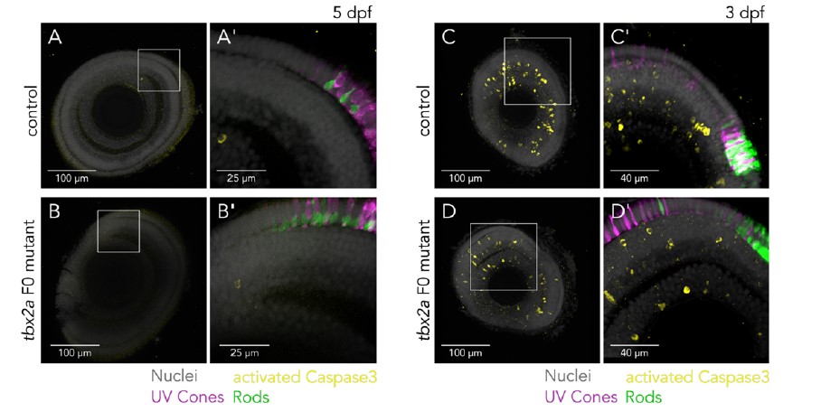
Reviewer Figure 1 - Assessment of apoptosis in tbx2a F0 mutants. (A-B) Confocal images of 5 dpf larval eyes of control (A and A’) and tbx2a F0 mutants (B and B’) counterstained with DAPI (grey) and immunolabeled against activated Caspase 3 (yellow) show sparse and dim labeling, restricted to cells located in the ciliary marginal zone, without clear differences between groups. (C-D) Confocal images of 3 dpf larval eyes of control (C and C’) and tbx2a F0 mutants (D and D’) immunolabeled against activated Caspase 3 show many positive cells, located in all retinal layers, as expected from physiological apoptosis at this stage of development and without clear differences between groups.
Furthermore, the additional single-cell RNA-seq datasets we have reanalyzed suggest that tbx2a and tbx2b are expressed by other retinal neurons and progenitors and not just photoreceptors (Reviewer Figure 2), further confounding attempts at the quantification of apoptosis specifically in photoreceptor progenitors.
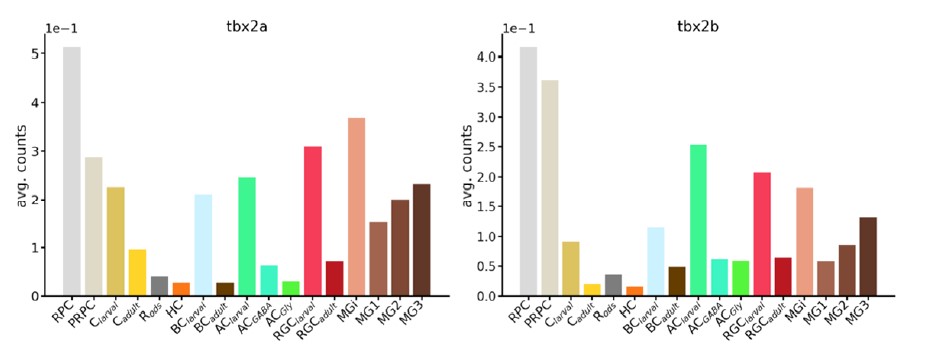
Reviewer Figure 2 – Expression of tbx2 paralogues across retinal cell types. The transcription factors tbx2a and tbx2b are expressed by many retinal cells. Plots show average counts across clusters in RNA-seq data obtained by Hoang et al. (2020).
At this stage, we consider that fully resolving this issue is important and will require considerably more work, which we will pursue in the future using full germline mutants and live-imaging experiments.
Reviewer #3 (Public Review):
Angueyra et al. tried to establish the method to identify key factors regulating fate decisions in the retinal visual photoreceptor cells by combining transcriptomic and fast genome editing approaches. First, they isolated and pooled five subtypes of photoreceptor cells from the transgenic lines in each of which a specific subtype of photoreceptor cells are labeled by fluorescence protein, and then subjected them to RNA-seq analyses. Second, by comparing the transcriptome data, they extracted the list of the transcription factor genes enriched in the pooled samples. Third, they applied CRISPR-based F0 knockout to functionally identify transcription factor genes involved in cell fate decisions of photoreceptor subtypes. To benchmark this approach, they initially targeted foxq2 and nr2e3 genes, which have been previously shown to regulate S-opsin expression and S-cone cell fate (foxq2) and to regulate rhodopsin expression and rod fate (nr2e3). They then targeted other transcription factor genes in the candidate list and found that tbx2a and tbx2b are independently required for UV-cone specification. They also found that tbx2a expressed in the L-cone subtype and tbx2b expressed in L-cones inhibit M-opsin gene expression in the respective cone subtypes. From these data, the authors concluded that the transcription factors Tbx2a and Tbx2b play a central role in controlling the identity of all photoreceptor subtypes within the retina.
Overall, the contents of this manuscript are well organized and technically sound. The authors presented convincing data, and carefully analyzed and interpreted them. It includes an evaluation of the presented data on cell-type specific transcriptome by comparing it with previously published ones. I think the current transcriptomic data will be a valuable platform to identify the genes regulating cell-type specific functions, especially in combination with the fast CRISPR-based in vivo screening methods provided here. I hope that the following points would be helpful for the authors to improve the manuscript appropriately.
1) The manuscript uses the word “FØ” quite often without any proper definition. I wonder how “Ø” should be pronounced - zero or phi? This word is not common and has not been used in previous publications. I feel the phrase “F0 knockout,” which was used in the paper cited by the authors (Kroll et al 2021), is more straightforward. If it is to be used in the manuscript, please define “FØ” and “CRISPR-FØ screening” appropriately, especially in the abstract.
We have made changes to replace “FØ” to “F0.” In our other citation (Hoshijima et al., 2019), “F0 embryo” was used throughout the paper. Following our references and Dr Kojima’s suggestion, we adopted “F0 mutant larva” as the most straightforward and less confusing term. We have also made changes in the abstract to define our approach more clearly and made appropriate changes throughout the manuscript.
2) Figure 1-supplement 1 shows that opn1mw4 has quite high (normalized) FPKM in one of the S-cone samples in contrast to the least (or no) expression in the M-cone samples, in which opn1mw4 is expected to be detected. The authors should address a possible origin of this inconsistent result for opn1mw4 expression as well as a technical limitation of using the Tg(opn1mw2:egfp) line for detection of opn1mw4 expression in the GFP-positive cells.
In Figure 1 - Supplement 1, we had attempted to provide a summarized figure of all phototransduction genes, but the big differences in expression levels — in particular, the high expression of opsins genes — forced us to use gene-by-gene normalization for display. Without normalization, the expression of opn1mw4 is very low across all samples, and its detection in that sole S-cone sample can likely be attributed to some degree of inherent noise in our methods. We have revised Figure 1 - Supplement 1: we find that we can avoid gene-by-gene normalization and still provide a good summary of the expression of phototransduction genes if the heatmap is broken down by gene families, which have more similar expression levels. In addition, we have added caveats to the use of the Tg(opn1mw2:egfp) line as our sole M-cone marker in the results section describing our RNA-seq approach, including our inability to provide data on Opn1mw4-expressing M cones.
3) The manuscript lacks a description of the sampling time point. It is well known that many genes are expressed with daily (or circadian) fluctuation (cf. Doherty & Kay, 2010 Annu. Rev. Genet.). For example, the cone-specific gene list in Fig.2C includes a circadian clock gene, per3, whose expression was reported to fluctuate in a circadian manner in many tissues of zebrafish including the retina (Kaneko et al. 2006 PNAS). It appears to be cone-specific at this time point of sample collection as shown in Fig.2, but might be expressed in a different pattern at other time points (eg, rod expression). The authors should add, at least, a clear description of the sampling time points so as to make their data more informative.
We have included this information in the materials and methods. We collected all our samples during the most active peak of the zebrafish circadian rhythm between 11am and 2pm (3h to 6h after light onset) to avoid the influence of circadian fluctuations in our analysis.
Author Response
Reviewer #1 (Public Review):
The authors use a newly developed object-space memory task comprising of a "Stable" version and "Overlapping" version where two objects are presented in two locations per trial in a square open field. Each version consists of 5 training trials of 5-min presentations of an object-space configuration, with both object locations staying constant across training trials in the Stable condition, and only one object location staying fixed in the Overlapping condition. Memory is tested in a test trial 24 hours later where the opposite configuration is presented - overlapping configuration presented for the Stable condition and stable configuration presented for the Overlapping condition - with the thesis that memory in this test trial for the Overlapping condition will depend on the accumulated memory of spatial patterns over the training trials, whereas memory for the test trial in the Stable condition can be due to episodic memory of last trial or accumulated memory. Memory is quantified using a Discrimination Index (DI), comparing the amount of time animals spend exploring the two object locations.
Here, animals in other groups are also presented with an interference trial equivalent to the test trial, to test if the memory of the Overlapping condition can be disrupted. The behavioral data show that for RGS14 over-expressing animals, memory in the Overlapping condition is diminished compared to controls with no interference or controls where over-expression is inhibited, whereas memory in the Stable condition is enhanced. This is interpreted as interference in semantic-like memory formation, whereas one-shot episodic memory is improved. The authors speculate that increased cortical plasticity should lead to increased and larger delta waves according to the sleep homeostasis hypothesis, and observe that instead increased cortical plasticity leads to less non-REM sleep and smaller delta waves, with more prefrontal neurons with slower firing rates (presumably more plastic neurons). They further report increased hippocampal-cortical theta coherence during task and REM sleep, increased NonREM oscillatory coupling, and changes in hippocampal ripples in RGS14 over-expressing animals.
While these results are interesting, there are several issues that need to be addressed, and the link between physiology and behavioral results is unclear.
1) The behavioral results rely on the interpretation that the Overlapping condition corresponds to semantic-like memory and the Stable condition corresponds to episodic-like memory. While the dissociation in memory performance due to interference seen in these two conditions is intriguing, the Stable condition can correspond not just to the memory of the previous trial but also accumulated memory of a stable spatial pattern over the 5 testing trials, similar to accumulated memory of a changing spatial pattern in the Overlapping pattern.
Yes! We completely agree on this. We do not claim the stable condition corresponds to episodic-like memory, instead we refer to it as simple memory, since it can be solved either way (one trial memory or cumulative memory). We now expanded this in the discussion to make it clearer.
Here, it is puzzling that in the behavioral control with no interference (Figure 1D), memory in the Stable and Overlapping condition is unchanged in the test trial, with the DI statistically at 0 in the test trial. In the original description of the Object Space task by the authors in the referenced paper, the measure of memory was a Discrimination Index significantly higher than 0 in both the Stable and Overlapping conditions. This discrepancy needs to be reconciled. Is the DI for the interference trial shown in Fig. S1 significantly different than 0? No statistics or description is provided in the figure legend here.
As mentioned above, we apologize that we oversimplified the description. The 24h interference trial would be what corresponds to the original test trial. We added a clarifying figure for comparison in S1 (bar graph in addition to the violin plot) and stats. Performance was for all groups and conditions above chance, replicating our previous results.
2) The physiology experiments compare Home cage (HC) conditions to the Object Space task (OS) throughout the manuscript. While some differences are seen in the control and RGS14 over-expressing animals, there is no comparison of the Stable vs. Overlapping condition in the physiology experiments. This precludes making explicit links between physiological observations and behavioral effects.
As also mentioned above, we have now added analysis exploring the detailed OS conditions. We would like to thank the reviewers for giving us the opportunity of doing so.
3) The authors speculate that learning will result in larger and more delta waves as per the synaptic homeostasis hypothesis. It should be noted here that an alternative hypothesis is that there should also be a selective increase in synaptic plasticity for learning and consolidation. The authors do observe that control animals show more frequent and higher-amplitude delta waves, but rather than enhancing this process, RGS14 animals with increased plasticity show the opposite effect. How can this be reconciled and linked with the behavioral data in the Stable and Overlapping condition?
In the context of the Object Space Task, we would expect all behavioural conditions (Stable and Overlapping) to induce synaptic changes since learning does occur also in the Stable condition (see also performance on 24h trial). Thus, especially homeostatic responses such as increase in delta amplitude, we would expect for all experiences independent if subtle statistical rules are presented or not. In contrast, detailed processing, extracting underlying regularities is rather proposed by the Sleep for Active Systems Consolidation Hypothesis to occur during hippocampal-cortical interactions in form of delta/ripple/spindle interactions (with different theories emphasising different types of interactions). As mentioned above, we now add a more specific analysis in this regards, where we can show that the two OS conditions that involve moving objects (where thus potentially statistical regularities can be extracted) show a higher percentage of ripples occurring after large slow oscillations in comparison to home cage or the simple learning condition Stable. In contrast, RGS14 already has higher participation in both control conditions, emphasising that in these animals all experiences are treated by the brain as significant learning condition, explaining the behavioural effect (increased interference due to better memory for the interference). Further, we expanded in the discussion how in RGS we sometimes see an enhancement of learning effects but sometimes see a more complex interaction of what we would expect from physiological learning.
Similarly, there is an increase in slower-firing neurons in RGS14 over-expressing animals. Slower-firing neurons have been proposed to be more plastic in the hippocampus based on their participation in learned hippocampal sequences, but appropriate references or data are needed to support the assertion that slower-firing neurons in the prefrontal cortex are more plastic.
As described above, we have expanded the discussion including other citations that also consider the cortex. We can show that our changes would be expected if one turns the cortex as plastic as the hippocampus.
4) It is noted that changing cortical plasticity influences hippocampal-cortical coupling and hippocampal ripples, suggesting a cortical influence on hippocampal physiological patterns. It has been previously shown that disrupting prefrontal cortical activity does alter hippocampal ripples and hippocampal theta sequences (Schmidt et al., 2019; Schmidt and Redish, 2021). The current results should be discussed in this context.
We would like to thank the reviewer for these suggestions, they are now incorporated in the manuscript.
Reviewer #2 (Public Review):
In this paper, the authors provide evidence to support the longstanding proposition that a dual-learning system/systems-level consolidation (hippocampus attains memories at a fast pace which are eventually transmitted to the slow-learning neocortex) allows rapid acquisition of new memories while protecting pre-existing memories. The authors leverage many techniques (behavior, pharmacology, electrophysiology, modelling) and report a host of behavioral and electrophysiological changes on induction of increased medial prefrontal cortex (mPFC) plasticity which are interesting and will be of significant interest to the broad readership.
The experimental design and analyses are convincing (barring some instances which are discussed below). The following recommendations will bolster the strength/quality of the manuscript:
1) Certain concerns regarding the interpretation and analysis of the behavioral data remain. The authors need to clarify if increased mPFC plasticity leads to only an increase in one-shot memory or 'also' interference of previous information. It seems that the behavioral results could also be explained by the more parsimonious explanation that one-shot memory is improved. Do the current controls tease apart these two scenarios?
We agree we cannot disentangle if one memory is just stronger than the other or if its an overwriting effect. We added this now to the discussion. Of note, we do not think it actually would be possible to distinguish these two effects behaviourally in rodents, or at least we cannot think of a fitting study design that would enable the contrast.
Additionally, the authors need to clarify why the 'no trial' and 'anisomycin' controls for the stable task perform at chance levels on exposure to a new object-place association on test day (Fig 1D).
Violin plots are sometimes hard to see. Here simple bar plots where you can see that the animals are not at chance at the 72h test in the control conditions.
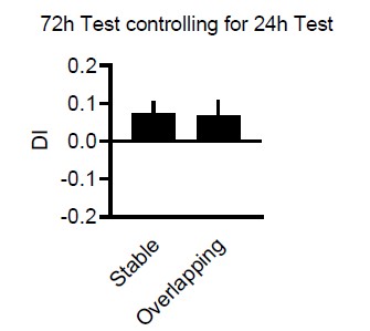
Finally, further description of how the discrimination index (exploration time of novel-exploration time of familiar/sum of both) is recommended i.e., in the stable condition, which 'object' is chosen as 'novel' (as both are in the same locations) for computing the index (Fig 1). Do negative DI values imply a neophobia to novel objects (and thus are a form of memory; this is also crucial because the modelling results (Fig 1E) use both neophilia and neophobia while negative discrimination indexes are considered similar to 0 for interpreting the behavioral results, as stated on page 3, lines 84-86?
We added this now to the methods (For Overlapping it is moved location – stable location, for Stable it is location-to-be-moved-at-test – stable location and for random which is assigned as moved and stable is random, and then for each divided by total time). We agree that neophilia/neophobia (especially changes in the distribution) can be an issue and have discussed it in detail in Schut et al NLM 2020 where we see difference in absolute beta values (thus controlling for philia/phobia differences). We also discuss there why it is difficult to control for this in the DI in more detail. In short, one could use absolute values but then it is difficult to determine what a group chance-level would look like. However, luckily here there is not issue since we did not observe difference in neophilic or phobic tendencies while running the experiments. Critically the interference trial (that can also function as simple test trial) confirms that as a group animals show positive DI and neophilia.
2) The authors report lower firing rates in RGS14414 animals during the task in Fig 2F. It is indeed remarkable how large the reported differences are. The authors need to rule out any differences in the behavioral state of the animals in the two groups during the task, i.e., rest vs. active exploration/movement dynamics. Are only epochs during the task while the animals interact with the objects used for computing the firing rates (same epochs as Fig 1)? If not, doing so will provide a useful comparison with Fig 1. Additionally, although the authors make the case for slow firing rate neurons being important for plasticity (based on Grosmark and Buzsaki, 2016), it is crucial to note that the firing rate dynamic (slow vs. fast) in that study for the hippocampus is defined based on the whole recorded session (predominated by sleep), indeed the firing rates of the two groups (slow vs. fast/plastic vs. rigid) during the task/maze-running do not differ in that study. Therefore, the results here seem incongruent with the Grosmark and Buzsaki paper. Since this finding is central to the main claim of the authors, it either warrants further investigation or a re-interpretation of their results.
As mentioned in the main points, we now added the firing rate analysis (including new groups splits) for wake in the sleep box, NREM and REM separately. Each time the same results are obtained. Currently, we do not yet have the tracking and video synchronization set-up, therefore we cannot split the task for specific behaviours.
However, we now also cite Buzsaki’s original log-normal brain review, where he first proposed the idea. There he also shows same effects as we do, in that the general firing rate distribution is the same for task and different sleep stages, just overall shifted. The analysis from Grosmark included more strigent subselection of neurons to be able to also argue that incorporation into run/replay-sequences could not have been biased by firing rate per se (instead of plasticity). However, the original proposition from Buzsaki does fit to our results. He further presents hippocampus vs cortex firing rates, which also confirm the idea (hippocampus more plastic and has slower firing rates). We included this figure above in the general comments. Further, we now expanded the discussion in this point.
3) A concern remains as to how many of the electrophysiological changes they observe (firing rate differences, LFP differences including coupling, sleep state differences, Figs. 2-4) support their main hypothesis or are a by-product of injection of RGS14414 (for instance, one might argue that an increased 'capability' to learn new information/more plasticity might lead to more NREM sleep for consolidation, etc.). The authors need to carefully interpret all their data in light of their main hypothesis, which will substantially improve the quality/strength of the manuscript.
We now expanded the discussion, included more structure and also include that we cannot disentangle if the cellular changes or sleep oscillation changes or an interaction of both is the cause of the result. Furthermore, we added that we cannot distinguish if the interference memory is stronger or actually overwrites the original training memory.
Reviewer #3 (Public Review):
The authors set out to test the idea that memories involve a fast process (for the acquisition of new information) and a slow process (where these memories are progressively transferred/integrated into more-long term storage). The former process involves the hippocampus and the latter the cerebral cortex. This 'dual-learning' system theoretically allows for new learning without causing interference in the consolidation of older memories. They test this idea by artificially increasing plasticity in the pre-limbic cortex and measuring changes in different learning/memory tasks. They also examined electrophysiological changes in sleep, as sleep is linked to memory formation and synaptic plasticity.
The strengths of the study include a) meticulous analyses of a variety of electrophysiological measurements b) a combination of neurobiological and computational tools c) a largely comprehensive analysis of sleep-based changes. Some weaknesses include questions about the technique for increasing cortical plasticity (is this physiological?) and the absence of some additional experiments that would strengthen the conclusions. However, overall, the findings appear to support the general idea under examination.
This study is likely to be very impactful as it provides some really new information about these important neural processes, as well as data that challenges popular ideas about sleep and synaptic plasticity.
We would like to thank the reviewer for these positive comments. Answers to the weaknesses are presented below in the recommendations for the authors.
Author Response
Reviewer 1 (Public Review):
To me, the strengths of the paper are predominantly in the experimental work, there's a huge amount of data generated through mutagenesis, screening, and DMS. This is likely to constitute a valuable dataset for future work.
We are grateful to the reviewer for their generous comment.
Scientifically, I think what is perhaps missing, and I don't want this to be misconstrued as a request for additional work, is a deeper analysis of the structural and dynamic molecular basis for the observations. In some ways, the ML is used to replace this and I think it doesn't do as good a job. It is clear for example that there are common mechanisms underpinning the allostery between these proteins, but they are left hanging to some degree. It should be possible to work out what these are with further biophysical analysis…. Actually testing that hypothesis experimentally/computationally would be nice (rather than relying on inference from ML).
We agree with the reviewer that this study should motivate a deeper biophysical analysis of molecular mechanisms. However, in our view, the ML portion of our work was not intended as a replacement for mechanistic analysis, nor could it serve as one. We treated ML as a hypothesis-generating tool. We hypothesized that distant homologs are likely to have similar allosteric mechanisms which may not be evident from visual analysis of DMS maps. We used ML to (a) extract underlying similarities between homologs (b) make cross predictions across homologs. In fact, the chief conclusion of our work is that while common patterns exist across homologs, the molecular details differ. ML provides tantalizing evidence to this effect. The conclusive evidence will require, as the reviewer rightly suggests, detailed experimental or molecular dynamics characterization. Along this line, we note that we have recently reported our atomistic MD analysis of allostery hotspots in TetR (JACS, 2022, 144, 10870). See ref. 41.
Changes to manuscript:<br /> “Detailed biophysical or molecular dynamics characterization will be required to further validate our conclusions(38).”
Reviewer 3 (Public Review):
However - at least in the manuscript's present form - the paper suffers from key conceptual difficulties and a lack of rigor in data analysis that substantially limits one's confidence in the authors' interpretations.
We hope the responses below address and allay the reviewer’s concerns.
A key conceptual challenge shaping the interpretation of this work lies in the definition of allostery, and allosteric hotspot. The authors define allosteric mutations as those that abrogate the response of a given aTF to a small molecule effector (inducer). Thus, the results focus on mutations that are "allosterically dead". However, this assay would seem to miss other types of allosteric mutations: for example, mutations that enhance the allosteric response to ligand would not be captured, and neither would mutations that more subtly tune the dynamic range between uninduced ("off) and induced ("on") states (without wholesale breaking the observed allostery). Prior work has even indicated the presence of TetR mutations that reverse the activity of the effector, causing it to act as a co-repressor rather than an inducer (Scholz et al (2004) PMID: 15255892). Because the work focuses only on allosterically dead mutations, it is unclear how the outcome of the experiments would change if a broader (and in our view more complete) definition of allostery were considered.
We agree with the reviewer that mutations that impact allostery manifest in many different ways. Furthermore, the effect size of these mutations runs the full gamut from subtle changes in dynamic range to drastic reversal of function. To unpack allostery further, allostery of aTF can be described, not just by the dynamic range, but by the actual basal and induced expression levels of the reporter, EC50 and Hill coefficient. Given the systemic nature of allostery, a substantial fraction of aTF mutations may have some subtle impact on one or more of these metrics. To take the reviewer’s argument one step further, one would have to accurately quantify the effect size of every single amino acid mutation on all the above properties to have a comprehensive sequence-function landscape of allostery. Needless to say, this is extremely hard! Resolution of small effect sizes is very difficult, even at high sequencing depth. To the best of our knowledge, a heroic effort approaching such comprehensive analysis has been accomplished so far only once (PMID: 3491352).
Our focus, therefore, was to screen for the strongest phenotypic impact on allostery i.e., loss of function. Mutations leading to loss of function can be relatively easily identified by cell-sorting. Because our goal was to compare hotspots across homologs, we surmised that loss of function mutations, given their strong phenotypic impact, are likely to provide the clearest evidence of whether allosteric hotspots are conserved across remote homologs.
The reviewer raised the point of activity-reversing mutations. Yes, there are activity reversing mutations in TetR. However, they represent an insignificant fraction. In the paper cited by the reviewer, there are 15 activity-reversing mutations among 4000 screened. Furthermore, the paper shows that activity-reversing in TetR requires two-tofour mutations, while our library is exclusively single amino acid substitutions. For these reasons, we did not screen for activity-reversing mutations. Nonetheless, we agree with the reviewer that screening for activity-reversing mutations across homologs would be very interesting.
The separation in fluorescence between the uninduced and induced states (the assay dynamic range, or fold induction) varies substantially amongst the four aTF homologs. Most concerningly, the fluorescence distributions for the uninduced and induced populations of the RolR single mutant library overlap almost completely (Figure 1, supplement 1), making it unclear if the authors can truly detect meaningful variation in regulation for this homolog.
Yes, the reviewer is correct that the fold induction ratio varies among the four aTF homologs. However, we note that such differences are common among natural aTFs. Depending on the native downstream gene regulated by the aTF, some aTFs show higher ligand-induced activation, and others are lower. While this is not a hard and fast rule, aTFs that regulate efflux pumps tend to have higher fold induction than those that regulate metabolic enzymes. In summary, the variation in fold induction among the four aTFs is not a flaw in experimental design nor indicates experimental inconsistency but is instead just an inherent property of protein-DNA interaction strength and the allosteric response of each aTF.
Among the four aTFs, wildtype RolR has the weakest fold induction (15-fold) which makes sorting the RolR library particularly challenging. To minimize false positives as much as possible, we require that dead mutant be present in (a) non-fluorescent cells after ligandinduction (b) non-fluorescent cells before ligand-induction (c) at least two out of the three replicates for both sorts. Additionally, for RolR specifically, we adjusted the nonfluorescent gate to be far more stringent than the other three aTFs (Fig. 1 – figure supplement 1). Furthermore, we assign residues as allosteric hotspots, not individual dead mutations. This buffers against false strong signals from stray individual dead mutations. Finally, the top interquartile range winnows them to residues showing strong consistent dead phenotype. As a result of these “safeguards” we have built in, the number of allosteric hotspots of RolR (57) is comparable to the other three aTFs (51, 53 and 48). This suggests that we are not overestimating the number of hotspots despite the weaker fold induction of RolR. We highlight in a new supplementary figure (Figure 1 – figure supplement 4) that changing the read count threshold from 5X to 10X produces near identical patterns of mutations suggesting that our results are also robust to changes in ready depth stringency.
Changes to manuscript: In response to the reviewer's comment, we have added the following sentence.
“We note that the lower fold induction (dynamic range) of RolR makes it particularly challenging to separate the dead variants from the rest.”
The methods state that "variants with at least 5 reads in both the presence and absence of ligand in at least two replicates were identified as dead". However, the use of a single threshold (5 reads) to define allosterically dead mutations across all mutations in all four homologs overlooks several important factors:
Depending on the starting number of reads for a given mutation in the population (which may differ in orders of magnitude), the observation of 5 reads in the gated nonfluorescent region might be highly significant, or not significant at all. Often this is handled by considering a relative enrichment (say in the induced vs uninduced population) rather than a flat threshold across all variants.
We regret the lack of clarity in our presentation. We wish to better explain the rationale behind our approach. First, we understand the reviewer’s point on considering relative enrichment to define a threshold. This approach works well in DMS experiments involving genetic selections, which is commonly the case, because activity scales well with selection stringency. One can then pick enrichment/depletion relative to the middle of the read count distribution as a measure of gain or loss of function.
Second, this strategy does not, in practice, work well for cell-sorting screens. While it may be tempting to think of cell sorting as comparably activity-scaled as genetic selections, in reality, the fidelity of fluorescent-activated cell sorters is much lower. Making quantitative claims of activity based on cell sorting enrichment can be risky. It is wiser to treat cell sorting results as yes/no binary i.e., does the mutation disrupt allostery or not. More importantly, the yes/no binary classification suffices for our need to identify if a certain mutation adversely impacts allosteric activity or not.
Third, the above argument does not imply that all mutations have the same effect size on allostery. They don’t. We capture the effect size on individual residues, not individual mutations, by counting the number of dead mutations at a residue position. This is an important consideration because it safeguards us from minor inconsistencies that inevitably arise from cell sorting.
Fourth, a variant to be classified as allosterically dead, it must be present both in uninduced and induced DNA-bound populations in at least two out of three replicates (four conditions total). This is a stringent criterion for selecting dead variants resulting in highly consistent regions of importance in the protein even upon varying read count thresholds. To the extent possible, we have minimized the possibility of false positive bleed-through.
Finally, two separate normalizations were performed on the total sequence reads to be able to draw a common read count threshold 1) between experimental conditions & replicates and 2) across proteins. First, total sequencing reads were normalized to 200k total across all sample conditions (presorted, -inducer, and +inducer) and replicates for each homolog, allowing comparisons within a single protein. Next, reads were normalized again to account for differences in the theoretical size of each protein’s single-mutant library, allowing for comparisons across proteins by drawing a commont readcount cutoff. For example, total sequencing reads of RolR (4,332 possible mutants) increased by 1.18x relative to MphR (3,667 possible mutants) for a total of 236k reads.
Changes to manuscript: We have provided substantial additional details in the Fluorescence-activated cell sorting and NGS preparation and analysis sections.
We also added the following in the main text.
“In other words, we use cell sorting as a binary classifier i.e., does the mutation disrupt allostery or not. We capture the effect size on individual residues, not individual mutations, by counting the number of dead mutations at a residue position. This is an important consideration because it safeguards us from minor inconsistencies that inevitably arise from cell sorting.”
Depending on the noise in the data (as captured in the nucleotide-specific q-scores) and the number of nucleotides changed relative to the WT (anywhere between 1-3 for a given amino acid mutation) one might have more or less chance of observing five reads for a given mutation simply due to sequencing noise.
All the reads considered in our analyses pass the Illumina quality threshold of Q-score ≥ 30 which as per Illumina represent “perfect reads with no errors or ambiguities”. This translates into a probability of 1 in 1000 incorrect base call or 99.9% base call accuracy.
We use chip-based oligonucleotides to build our DMS library, which allows us to prespecify the exact codon that encodes a point mutation. This means the nucleotide count and protein count are the same. The scenario referred to by the reviewer i.e., “anywhere between 1-3 for a given amino acid mutation” only applies to codon randomized or errorprone PCR library generation. We regret if the chip-based library assembly part was unclear.
Depending on the shape and separation of the induced (fluorescent) and uninduced (non-fluorescent) population distributions, one might have more or less chance of observing five reads by chance in the gated non-fluorescent region. The current single threshold does not account for variation in the dynamic range of the assay across homologs.
We have addressed the concern raised by the reviewer on fluorescent population distributions in answers to questions 10 and 11.
The reviewer makes an important point about the choice of sequencing threshold. We use the sequencing threshold to simply make a binary choice for whether a certain variant exists in the sorted population or not. We do not use the sequencing reads as to scale the activity of the variant. To address the reviewer's comment, we have included a new supplementary figure (Fig 1 – figure supplement 4) where we compare the data by adjust the threshold two levels – 5 and 10 reads. As is evident in the new figure, the fundamental pattern of allosteric hotspots and the overall data interpretation does not change.
TetR: 5x – 53 hotspots, 10x – 51 hotspots
TtgR: 5x – 51 hotspots, 10x – 51 hotspots
MphR: 5x – 48 hotspots, 10x – 48 hotspots
RolR: 5x – 57 hotspots, 10x – 60 hotspots
In other words, changing the threshold to be more or less strict may have a modest impact on the overall number of hotspots in the dataset. Still, the regions of functional importance are consistent across different thresholds. We have expanded the discussion in the manuscript to address this point.
Changes to manuscript: We have now included a new supplementary comparing hotspot data at two thresholds: Figure 1 – figure supplement 4.
We also added the following in the main text.
“To assess the robustness of our classification of hotspots, we determined the number of hotspots at two different sequencing thresholds – 5x and 10x. At 5x and 10x, the number of hotspots are – TetR: 53, 51; TtgR: 51, 51; MphR: 48, 48 and RolR: 57,60, respectively. Changing the threshold has a modest impact on the overall number of hotspots and the regions of functional importance are consistent at both thresholds”
The authors provide a brief written description of the "weighted score" used to define allosteric hotspots (see y-axis for figure 1B), but without an equation, it is not clear what was calculated. Nonetheless, understanding this weighted score seems central to their definition of allosteric hotspots.
We regret the lack of clarity in our presentation. The weighted score was used to quantify the “deadness” of every residue position in the protein. At each position in the protein, the number of mutations that inhibited activity was summed up and the ‘deadness’ of each mutation was weighted based on how many replicates is appeared to inactivate the protein. Weighted score at each residue position is given by

Where at position x in the protein, D1 is the number of mutations dead in one replicate only, D2 is the number of mutations dead in 2 replicates, D3 is the number of mutations dead in 3 replicates, and Total is the total number of variants present in the data set (based on sequencing data). Any dead mutation that is seen in only one replicate is discarded and does not contribute to the “deadness” of the residue. Mutations seen in two and three replicates contribute to the score. We have included a new supplementary figure (Fig. 1 – figure supplement 2) to give the reader a detailed heatmap of all mutations and their impact for each protein.
Changes to manuscript: The weighted scoring scheme is now described in greater detail under Materials and Methods in the “NGS preparation and analysis” section.
The authors do not provide some of the standard "controls" often used to assess deep mutational scanning data. For example, one might expect that synonymous mutations are not categorized as allosterically dead using their methods (because they should still respond to ligand) and that most nonsense mutations are also not allosterically dead (because they should no longer repress GFP under either condition). In general, it is not clear how the authors validated the assay/confirmed that it is giving the expected results.
As we state in response to question 12, we use chip-based oligonucleotides to build our DMS library, which allows us to pre-specify the exact codon that encodes a point mutation. We have no synonymous or nonsense mutations in our DMS library. Each protein mutation is encoded by a single unique codon. The only stop codon is at 3’end of the gene.
The authors performed three replicates of the experiment, but reproducibility across replicates and noise in the assay is not presented/discussed.
Changes to manuscript: A new supplementary table (Table 1) is now provided with the pairwise correlation coefficients between all replicates for each protein.
In the analysis of long-range interactions, the authors assert that "hotspot interactions are more likely to be long-range than those of non-hotspots", but this was not accompanied by a statistical test (Figure 2 - figure supplement 1).
In response to the reviewer's comment, we now include a paired t-test comparing nonhotspots and hotspots with long-range interactions in the main text.
Changes to manuscript: In all four aTFs, hotspots constituted a higher fraction of LRIs than non-hotspots (Figure 2 – figure supplement 1; P = 0.07).
Author Response
Reviewer #1 (Public Review):
In this study, the authors describe an elegant genetic screen for mutants that suppress defects of MCT1 deletions which are deficient in mitochondrial fatty acid synthesis. This screen identified many genes, including that for Sit4. In addition, genes for retrograde signaling factors (Rtg1, Rtg2 and Rtg3), proteins influencing proteasomal degradation (Rpn4, Ubc4) or ribosomal proteins (Rps17A, Rps29A) were found. From this mix of components, the authors selected Sit4 for further analysis. In the first part of the study, they analyzed the effect of Sit4 in context of MCT1 mutant suppression. This more specific part is very detailed and thorough, the experiments are well controlled and convincing. The second, more general part of the study focused on the effect of Sit4 on the level of the mitochondrial membrane potential. This part is of high general interest, but less well developed. Nevertheless, this study is very interesting as it shows for the first time that phosphate export from mitochondrial is of general relevance for the membrane potential even in wild type cells (as long as they live from fermentation), that the Sit4 phosphatase is critical for this process and that the modulation of Sit4 activity influences processes relying on the membrane potential, such as the import of proteins into mitochondria. However, some aspects should be further clarified.
1) It is not clear whether Sit4 is only relevant under fermentative conditions. Does Sit4 also influence the membrane potential in respiring cells? Fig. S2D shows the membrane potential in glucose and raffinose. Both carbon sources lead to fermentative growths. The authors should also test whether Sit4 levels influence the membrane potential when cells are grown under respirative conditions, such in ethanol, lactate or glycerol. Even if deletions of Sit4 affect respiration, mutants with altered activity can be easily analyzed.
sit4Δ cells fail to grow on nonfermentable media as shown by us (Figure 2—figure supplement 1C) and others (Arndt et al., 1989; Dimmer et al., 2002; Jablonka et al., 2006). In our opinion, the exact reason is unclear, but there is an interesting observation that addition of aspartate can partially restore growth on ethanol (Jablonka et al., 2006). Despite the lack of thorough investigation on this sit4Δ defect, an early study speculated that this defect could be related to the cAMP-PKA pathway (Sutton et al., 1991). This study pointed out genetic interactions of SIT4 with multiple genes in cAMP-PKA (Sutton et al., 1991). In addition, sit4Δ cells have similar phenotypes as those cAMP-PKA null mutants, such as glycogen accumulation, caffeine resistant, and failure to grow on nonfermentable media (Sutton et al., 1991). We have not found sit4Δ mutants that could grow on nonfermentable media based on literature search.
2) The authors should give a name to the pathway shown in Fig. 4D. This would make it easier to follow the text in the results and the discussion. This pathway was proposed and characterized in the 90s by George Clark-Walker and others, but never carefully studied on a mechanistic level. Even if the flux through this pathway cannot be measured in this study, the regulatory role of Sit4 for this process is the most important aspect of this manuscript.
We now refer this mechanism as the mitochondrial ATP hydrolysis pathway.
3) To further support their hypothesis, the authors should show that deletion of Pic1 or Atp1 wipes out the effect of a Sit4 deletion. In these petite-negative mutants, the phosphate export cycle cannot be carried out and thus, Sit4, should have no effect.
The mitochondrial phosphate transport activity is electroneutral as it also pumps a proton together with inorganic phosphate. The F1 subunit of the ATP synthase (Atp1 and Atp2) is suggested among many literatures to be responsible for the ATP hydrolysis. We performed tetrad dissection to generate atp1Δ or atp2Δ in pho85Δ background. After streaking the single colony to a fresh plate, we noticed that atp1Δ mct1Δ and atp2Δ mct1Δ cells are lethal, and knocking out PHO85 rescued this synthetic lethality. It is not surprising that atp1Δ mct1Δ or atp2Δ mct1 Δ cells are lethal since the F1 subunit is important to generate a minimum of MMP in mct1 Δ cells when the ETC is absent (i.e., rho0 cells). However, knocking out PHO85 can generate MMP independent of F1 subunit of ATP synthase, which is suggested by the viable atp1Δ mct1Δ pho85Δ and atp2Δ mct1Δ pho85Δ cells. There are many ATPases in the mitochondrial matrix that could hydrolyze ATP for ADP/ATP carrier to generate MMP theoretically. However, we do not currently know exactly which ATPase(s) is activated by phosphate starvation. This data is now included as Figure 5—figure supplement 1F-G.
4) What is the relevance of Sit4 for the Hap complex which regulates OXPHOS gene expression in yeast? The supplemental table suggests that Hap4 is strongly influenced by Sit4. Is this downstream of the proposed role in phosphate metabolism or a parallel Sit4 activity? This is a crucial point that should be addressed experimentally.
To investigate the role of the Hap complex in MMP generation in sit4Δ cells, we overexpressed and knocked out HAP4, the catalytic subunit of the Hap complex, separately in wild-type and sit4Δ cells. We confirmed the HAP4 overexpression by the enriched abundance of ETC complexes as shown in the BN-PAGE (Figure 2—figure supplement 1E). However, we did not observe any rescue of ETC or ATP synthase in mct1Δ cells when HAP4 was overexpressed. The enriched level of ETC complexes by HAP4 overexpress is not sufficient to rescue the MMP (Figure 2—figure supplement 1F).
Next, we knocked out HAP4 in sit4Δ cells. Knocking out SIT4 could still increase MMP in hap4Δ cells with a much-reduced magnitude, which phenocopied ETC subunit and RPO41 deletion in sit4Δ cells (Figure 2—figure supplement 1G).
In conclusion, the Hap complex is involved in the MMP increase when SIT4 is absent. However, it is not sufficient to increase MMP by overexpressing HAP4. The Hap complex discussion is now included in the manuscript, and the data is presented as Figure 2—figure supplement 1E-G.
5) The authors use the accumulation of Ilv2 precursors as proxy for mitochondrial protein import efficiency. Ilv2 was reported before as a protein which, if import into mitochondria is slow, is deviated into the nucleus in order to be degraded (Shakya,..., Hughes. 2021, Elife). Is it possible that the accumulation of the precursor is the result of a reduced degradation of pre-Ilv2 in the nucleus rather than an impaired mitochondrial import? Since a number of components of the ubiquitin-proteasome system were identified with Sit4 in the same screen, a role of Sit4 in proteasomal degradation seems possible. This should be tested.
We thank the reviewer for pointing out this potential caveat with our Ilv2-FLAG reporter. With limited search and tests, we could not find another reporter that behaves like Ilv2FLAG. The reason Ilv2-FLAG is a perfect reporter for this study is because in wild-type cells, Ilv2-FLAG is not 100% imported. Therefore, we could demonstrate that mitochondria with higher MMP import more efficiently. Unfortunately, all of the mitochondrial proteins that we tested could efficiently import in wild-type cells. To identify other suitable mitochondrial proteins that behave like Ilv2-FLAG, we would need to conduct a more comprehensive screen.
To address the concern of the involvement of protein degradation in obscuring the interpretation of Ilv2-FLAG import, we performed two experiments. First, we measured the proteasomal activity in wild-type and our mutants using a commercial kit (Cayman). We did not observe a statistically significant difference in 20S proteasomal activity between wild-type and sit4Δ cells.
In the second experiment, we reduced the MMP of sit4 cells using CCCP treatment and measured the Ilv2-FLAG import. We first treated sit4Δ cells with different dosage of CCCP for six hours and measured their MMP. sit4Δ cells treated with 75 µM CCCP had comparable MMP to wild-type cells. When we treated sit4Δ cells with higher concentrations of CCCP, most of the cells did not survive after six hours. Next, we performed the Ilv2-FLAG import assay. We observed similar level of unimported Ilv2FLAG (marked with *) in sit4Δ cells treated with 75 µM CCCP. This result confirms that sit4Δ cells have similar Ilv2-FLAG turnover mechanism and activity as the wild-type cells, because when we lower the MMP in sit4Δ background we observe a similar level of unimported Ilv2-FLAG. We thus feel confident in concluding that the Ilv2-FLAG import results are indeed an accurate proxy for MMP level. These data are now included as Figure 1—figure supplement 1H-J in the manuscript.
Author response image 1.
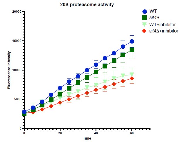
Reviewer #2 (Public Review):
This study reports interesting findings on the influence of a conserved phosphatase on mitochondrial biogenesis and function. In the absence of it, many nucleus-encoded mitochondrial proteins among which those involved in ATP generation are expressed much better than in normal cells. In addition to a better understanding of th mechanisms that regulate mitochondrial function, this work may help developing therapeutic strategies to diseases caused by mitochondrial dysfunction. However there are a number of issues that need clarification.
1) The rationale of the screening assay to identify genes required for the gene expression modifications observed in mct1 mutant is not clear. Indeed, after crossing with the gene deletion libray, the cells become heterozygote for the mct1 deletion and should no longer be deficient in mtFAS. Thank you for clarifying this and if needed adjust the figure S1D to indicate that the mated cells are heterozygous for the mct1 and xxx mutations.
We updated the methods section and the graphic for the genetic screen to clarify these points within the SGA workflow overview. After we created the heterozygote by mating mct1Δ cells with the individual KO cells in the collection, these diploids underwent sporulation and selection for the desired double KO haploid. As a result, the luciferase assay was performed in haploid cells with MCT1 and one additional non-essential gene deleted.
2) The tests shown in Fig. S1E should be repeated on individual subclones (at least 100) obtained after plating for single colonies a glucose culture of mct1 mutant, to determine the proportion of cells with functional (rho+) mtDNA in the mct1 glucose and raffinose cultures. With for instance a 50% proportion of rho- cells, this could substantially influence the results of the analyses made with these cells (including those aiming to evaluate the MMP).
We agree that this would provide a more confident estimate for population-level characterization of these colonies. It is important to note that we randomly chose 10 individual subclones, and 100% of these colonies were verified to be rho+. This suggests the population has functional mtDNA, and thus felt confident in the identity of our populations.
3) The mitochondria area in mct1 cells (Fig.S1G) does not seem to be consistent with the tests in Fig. 1C. that indicate a diminished mitochondrial content in mct1 cells vs wild-type yeast. A better estimate (by WB for instance) of the mitochondrial content in the analyzed strains would enable to better evaluate MMP changes monitored with Mitotracker since the amount of mitochondria in cells correlate with the intensity of the fluorescence signal.
As this reviewer pointed out, we quantified mitochondrial area based on Tom70-GFP signal. This measurement is quantified by mitochondrial area over cell size. Cell size is an important parameter when measuring organelle size as most of the organelles scale up and down with the cell size. mct1Δ cells generally have smaller cell size than WT cells. Therefore, the mitochondrial area of mct1Δ cells was not significantly different from WT cells when scaled to cell size. We believe this is the best method to compare mitochondrial area. As for quantifying MMP from these microscopy images, we measured the average MitoTracker Red fluorescence intensity of each mitochondria defined by Tom70-GFP. This method inherently normalizes to subtract the influence of mitochondria area when quantifying MMP.
4) Page 12: "These data demonstrate that loss of SIT4 results in a mitochondrial phenotype suggestive of an enhanced energetic state: higher membrane potential, hyper-tubulated morphology and more effective protein import." Furthermore, the sit4 mutant shows higher levels of OXPHOS complexes compared to WT yeast.
Despite these beneficial effects on mitochondria, the sit4 deletion strain fails to grow on respiratory substrates. It would be good to know whether the authors have some explanation for this apparent contradiction.
We agree that this was initially puzzling. We provide a more complete explanation above (see comments to reviewer #1 - major concern #1). Briefly, the growth deficiency in non-fermentable media with sit4Δ cells was reported and studied by multiple groups (Arndt et al., 1989; Dimmer et al., 2002; Jablonka et al., 2006). These seems to indicate that sit4Δ cells contain more ETC complexes and more OCR but cannot respire on nonfermentable carbon source. However, we do not think there is yet a clear explanation for this phenotype. One interesting observation reported is the addition of aspartate partly restoring cells’ growth on ethanol (Jablonka et al., 2006). One early study speculates that this defect could be related to the cAMP-PKA pathway. Sutton et al. pointed out genetic interactions with sit4 and multiple genes in cAMP-PKA (Sutton et al., 1991). In addition, sit4Δ cells have similar phenotypes as those cAMP-PKA null mutants, such as glycogen accumulation, caffeine resistance, and failure to grow on non-fermentable media. However, to keep this manuscript succinct, we opted to stay focused on MMP.
Reviewer #3 (Public Review):
In this study, the authors investigate the genetic and environmental causes of elevated Mitochondrial Membrane Potential (MMP) in yeast, and also some physiological effects correlated with increased MMP.
The study begins with a reanalysis of transcriptional data from a yeast mutant lacking the gene MCT1 whose deletion has been shown to cause defects in mitochondrial fatty acid synthesis. The authors note that in raffinose mct1del cells, unlike WT cells, fail to induce expression of many genes that code for subunits of the Electron Transport Chain (ETC) and ATP synthase. The deletion of MCT1 also causes induction of genes involved in acetyl-CoA production after exposure to raffinose. The authors therefore conduct a screen to identify mutants that suppress the induction of one of these acetylCoA genes, Cit2. They then validate the hits from this screen to see which of their suppressor mutants also reduce expression in four other genes induced in a mct1del strain. This yielded 17 genes that abolished induction of all 5 genes tested in an mct1del background during growth on raffinose.
The authors chose to focus on one of these hits, the gene coding for the phosphatase SIT4 (related to human PP6) which also caused an increase in expression of two respiratory chain genes. The authors then investigated MMP and mitochondrial morphology in strains containing SIT4 and MCT1 deletions and surprisingly saw that sit4del cells had highly elevated MMP, more reticular mitochondria, and were able to fully import the acetolactate synthase protein Ilv2p and form ETC and ATP synthase complexes, even in cells with an mct1del background, rescuing the low MMP, fragmented mitochondria, low import of Ilv2 and an inability to form ETC and ATP synthase complexes phenotypes of the mct1del strain. Surprisingly, the authors find that even though MMP is high and ETC subunits are present in the sit4del mct1del double deletion strain, that strain has low oxygen consumption and cannot grow under respiratory conditions, indicating that the elevated MMP cannot come from fully functional ETC subunits. The authors also observe that deleting key subunits of ETC complex III (QCR2) and IV (COX5) strongly reduced the MMP of the sit4del mutant, which would suggest that the majority of the increase in MMP of the sit4del mutant was dependant on a partially functional ETC. The authors note that there was still an increase in MMP in the qcr2del sit4del and cox4del sit4del strains relative to qcr2del and cox4del strains indicating that some part of the increase in MMP was not dependent on the ETC.
The authors dismiss the possibility that the increase in MMP could have been through the reversal of ATP synthase because they observe that inhibition of ATP synthase with oligomycin led to an increase of MMP in sit4del cells. Indicating that ATP synthase is operating in a forward direction in sit4del cells.
Noting that genes for phosphate starvation are induced in sit4del cells, the authors investigate the effects of phosphate starvation on MMP. They found that phosphate starvation caused an increase in MMP and increased Ilv2p import even in the absence of a mitochondrial genome. They find that inhibition of the ADP/ATP carrier (AAC) with bongkrekic acid (BKA) abolishes the increase of MMP in response to phosphate starvation. They speculate that phosphate starvation causes an increase in MMP through the import and conversion of ATP to ADP and subsequent pumping of ADP and inorganic phosphate out of the mitochondria.
They further show that MMP is also increased when the cyclin dependent kinase PHO85 which plays a role in phosphate signaling is deleted and argue that this indicates that it is not a decrease in phosphate which causes the increase in MMP under phosphate starvation, but rather the perception of a decrease in phosphate as signalled through PHO85. Unlike in the case of SIT4 deletion, the increase in MMP caused by the deletion of pho85 is abolished when MCT1 is deleted.
Finally they show an increase in MMP in immortalized human cell lines following phosphate starvation and treatment with the phosphate transporter inhibitor phosphonoformic acid (PFA). They also show an increase in MMP in primary hepatocytes and in midgut cells of flies treated with PFA.
The link between phosphate starvation and elevated MMP is an important and novel finding and the evidence is clear and compelling. Based on their experiments in various mammalian contexts, this link appears likely to be generalizable, and they propose and begin to test an interesting hypothesis for how MMP might occur in response to phosphate starvation in the absence of the Electron Transport Chain.
The link between phosphate starvation and deletion of the conserved phosphatase SIT4 is also interesting and important, and while the authors' experiments and analysis suggest some connection between the two observations, that connection is still unclear.
Major points
Mitotracker is great fluorescent dye, but it measures membrane potential only indirectly. There is a danger when cells change growth rates, ion concentrations, or when the pH changes, all MMP indicating dyes change in fluorescence: their signal is confounded Change in phosphate levels can possibly do both, alter pH and ion concentrations. Because all conclusions of the manuscript are based on a change in MMP, it would be a great precaution to use a dye-independent measure of membrane potential, and confirm at least some key results.
Mitochondrial MMP does strongly influence amino acid metabolism, and indeed the SIT4 knockout has a quite striking amino acid profile, with histidine, lysine, arginine, tyrosine being increased in concentration. http://ralser.charite.de/metabogenecards/Chr_04/YDL047W.html Could this amino acid profile support the conclusions of the authors? At least lysine and arginine are down in petites due to a lack of membrane potential and iron sulfur cluster export.- and here they are up. Along these lines, according to the same data resource, the knock-outs CSR2, ASF1, SSN8, YLR0358 and MRPL25 share the same metabolic profile. Due to limited time I did not re-analyse the data provided by the authors- but it would be worth checking if any of these genes did come up in the screens of the authors.
We tested the mutants within the same cluster as SIT4 shown in this paper from the deletion collection and measured their MMP. yrl358cΔ cells have similar high MMP as observed in sit4Δ cells. However, this gene has a yet undefined function. Beyond YRL358C, we did not observe similar MMP increases in other gene deletions from this panel, which does not support the notion that amino acids such as histidine, lysine, arginine, or tyrosine play a determining effect in driving MMP.
The media condition and strain used in the suggested paper is very different from what we used in our study. Instead of growing prototrophic cells in minimal media without any amino acids, we used auxotrophic yeast strains and grew them in media containing complete amino acids. So far, none of the other defects or signaling associated with SIT4 deletion could influence MMP as much as the phosphate signaling. We interpret these data to support the hypothesis that the MMP observation in sit4Δ cells is connected with the phosphate signaling as illustrated by the second half of the story in our manuscript.
Author reponse image 2.
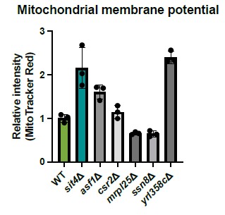
One important claim in the manuscript attempts to explain a mechanism for the MMP increase in response to phosphate starvation which is independent of the ETC and ATP synthase.
It seems to me the only direct evidence to support this claim is that inhibition of the AAC with BKA stops the increase of mitotracker fluorescence in response to phosphate starvation in both WT and rho0 cells (Figs 4B and 4C). It would strengthen the paper if the authors could provide some orthogonal evidence.
This is a similar comment as raised by reviewer #1 - major concern #3. We refer the reviewer to our discussion and the new data above. Briefly, we do not think F1 subunit is responsible for the ATP hydrolysis activity to generate MMP in phosphate depleted situation. We believe there are additional ATPase(s) in the mitochondrial matrix that can be utilized to couple to ADP/ATP carrier for MMP generation during phosphate starvation. However, we have not identified the relevant ATPase(s) at this point, and it is likely that multiple ATPases could contribute to this activity.
Introduction/Discussion The author might want to make the reader of the article aware that the 'reversal' of the ATP synthase directionality -i.e. ATP hydrolysis by the ATP synthase as a mechanism to create a membrane potential (in petites), has always been a provocative idea - but one that thus far could never be fully substantiated. Indeed some people that are very familiar with the topic, are skeptical this indeed happens. For instance, Vowinckel et al 2021 (PMID: 34799698) measured precise carbon balances for peptide cells, and found no evidence for a futile cycle - peptides grow slower, but accumulate the same biomass from glucose as peptides that re-evolve at a fast growth rate . Perhaps the manuscript could be updated accordingly.
We thank the reviewer for pointing out this additional relevant study. We have rephased the referenced sentence in the introduction. The MMP generation in phosphate starvation is independent of the F1 portion of ATP synthase. Therefore, our data neither supports or refutes either of these arguments.
In the introduction and conclusion there is discussion of MMP set points. In particular the authors state:
"Critically, we find that cells often prioritize this MMP setpoint over other bioenergetic priorities, even in challenging environments, suggesting an important evolutionary benefit."
This does not seem to be consistent with the central finding of the manuscript that MMP changes under phosphate starvation. MMP doesn't seem so much to have a 'set point' but rather be an important physiological variable that reacts to stimuli such as phosphate starvation.
The reviewer raises a rational alternative hypothesis to the one that we have proposed. In reality, both of these are complete speculations to explain the data and we can’t think of any way to test the evolutionary basis for the mechanisms that we describe. We recognize that untested/untestable speculative arguments have limitations and there are viable alternative hypotheses. We have softened our language to ensure that it is clear that this is only a speculation.
The authors suggest that deletion of Pho85 causes an increase in MMP because of cellular signaling. However, they also state in the conclusion:
"Unlike phosphate starvation, the pho85D mutant has elevated intracellular phosphate concentrations. This suggests that the phosphate effect on MMP is likely to be elicited by cellular signaling downstream of phosphate sensing rather than some direct effect of environmental depletion of phosphate on mitochondrial energetics."
The authors should cite the study that shows deletion of PHO85 causes increased intracellular phosphate concentrations. It also seems possible that the 'cellular signaling' that causes the increase in MMP could be a result of this increase in intracellular phosphate concentrations, which could constitute a direct effect of an environmental overload of phosphate on mitochondrial energetics.
We now cited the literature that shows higher intracellular phosphate in pho85Δ cells (Gupta et al., 2019; Liu et al., 2017). Depleting phosphate in the media drastically reduced intracellular phosphate concentration, which is the opposing situation as pho85Δ cells. Nevertheless, we observed higher MMP in either situation. We concluded from these two observations that the increase in MMP is a response to the signaling activated by phosphate depletion rather than the intracellular phosphate abundance.
Related to this point, in the conclusion, the authors state:
"We now show that intracellular signaling can lead to an increased MMP even beyond the wild-type level in the absence of mitochondrial genome."
In sum, the data shows that signaling is important here- but signaling alone is only the message - not the biophysical process that creates a membrane potential. The authors then could revise this slightly.
We have rephrased this sentence as suggested, which now reads “We now show that intracellular signaling triggers a process that can lead to an increased MMP even beyond the wild-type level in the absence of mitochondrial genome”.
The authors state in the conclusion that
"We first made the observation that deletion of the SIT4 gene, which encodes the yeast homologue of the mammalian PP6 protein phosphatase, normalized many of the defects caused by loss of mtFAS, including gene expression programs, ETC complex assembly, mitochondrial morphology, and especially MMP (Fig. 1)"
The data shown though indicates that a defect in mtFAS in terms of MMP, deletion of SIT4 causes a huge increase (and departure away from normality) whether or not mct1 is present (Fig 1D)
We changed the word “normalized” to “reversed”. In the discussion section, we also emphasized that many of these increases are independent of mitochondrial dysfunction induced by loss of mtFAS.
The language "SIT4 is required for both the positive and negative transcriptional regulation elicited by mitochondrial dysfunction" feels strong. SIT4 seems to influence positive transcriptional regulation in response to mitochondrial dysfunction caused by MCT1 deletion (but may not be the only thing as there appears to be an increase in CIT2 expression in a sit4del background following a further deletion of MCT1). In terms of negative regulation, SIT4 deletion clearly affects the baseline, but MCT1 deletion still causes down regulation of both examples shown in Fig 1B, showing that negative transcriptional regulation can still occur in the absence of SIT4. The authors might consider showing fold change of expression as they do in later figures (Figs 4B and C) to help the reader evaluate the quantitative changes they demonstrate.
We now displayed the fold change as suggested. This sentence now reads “These data suggest that SIT4 positively and negatively influences transcriptional regulation elicited by mitochondrial dysfunction”.
The authors induce phosphate starvation by adding increasing amounts of potassium phosphate monobasic at a pH of 4.1 to phosphate dropout media supplemented with potassium. The authors did well to avoid confounding effects of removing potassium. The final pH of YNB is typically around 5.2. Is it possible that the authors are confounding a change in pH with phosphate starvation? One would expect the media in the phosphate starvation condition to have a higher pH than the phosphate replacement or control media. Is a change in pH possibly a confounding factor when interpreting phosphate starvation? Perhaps the authors could quantify the pH of the media they use for the experiment to understand how much of a factor that could be. One needs to be careful with Miotracker and any other fluorescent dye when pH changes. Albeit having constraints on its own, MitoLoc as a protein rather than small molecule marker of MMP might be a good complement.
We followed the protocol used by many other studies that depleted phosphate in the media. The reason we and others adjusted the media without inorganic phosphate to a pH of 4.1 is because that is the pH of phosphate monobasic. From there, we could add phosphate monobasic to create +Pi media without changing the media pH. Therefore, media containing different concentrations of phosphate all have the exact same pH. We now emphasize that all media containing different levels of inorganic phosphate have the same pH to the manuscript to eliminate such concern (see page 18).
Even though all media have the similar pH, we also provided complementary data using a parallel approach to measure the MMP by assessing mitochondrial protein import as demonstrated previously with Ilv2-FLAG, which shares the same principle as mitoLoc.
Reference
Arndt, K. T., Styles, C. A., & Fink, G. R. (1989). A suppressor of a HIS4 transcriptional defect encodes a protein with homology to the catalytic subunit of protein phosphatases. Cell, 56(4), 527–537. https://doi.org/10.1016/00928674(89)90576-X
Dimmer, K. S., Fritz, S., Fuchs, F., Messerschmitt, M., Weinbach, N., Neupert, W., & Westermann, B. (2002). Genetic basis of mitochondrial function and morphology in Saccharomyces cerevisiae. Molecular Biology of the Cell, 13(3), 847–853. https://doi.org/10.1091/mbc.01-12-0588
Gupta, R., Walvekar, A. S., Liang, S., Rashida, Z., Shah, P., & Laxman, S. (2019). A tRNA modification balances carbon and nitrogen metabolism by regulating phosphate homeostasis. ELife, 8, e44795. https://doi.org/10.7554/eLife.44795
Jablonka, W., Guzmán, S., Ramírez, J., & Montero-Lomelí, M. (2006). Deviation of carbohydrate metabolism by the SIT4 phosphatase in Saccharomyces cerevisiae. Biochimica et Biophysica Acta (BBA) - General Subjects, 1760(8), 1281–1291. https://doi.org/10.1016/j.bbagen.2006.02.014
Liu, N.-N., Flanagan, P. R., Zeng, J., Jani, N. M., Cardenas, M. E., Moran, G. P., & Köhler, J. R. (2017). Phosphate is the third nutrient monitored by TOR in Candida albicans and provides a target for fungal-specific indirect TOR inhibition. Proceedings of the National Academy of Sciences, 114(24), 6346–6351. https://doi.org/10.1073/pnas.1617799114
Sutton, A., Immanuel, D., & Arndt, K. T. (1991). The SIT4 protein phosphatase functions in late G1 for progression into S phase. Molecular and Cellular Biology, 11(4), 2133–2148.